Page 1
DETERMINATION OF THE MINIMUM IGNITION
ENERGY (MIE) OF PREMIXED PROPANE/AIR
By
My Ngo
A thesis submitted in partial fulfilment of the requirements for the
Master of Science Program in Process Safety Technology
Department of Physics and Technology
University of Bergen, Norway
June 2009
Page 2
i
TABLE OF CONTENTS
TABLE OF CONTENTS .......................................................................................................... i
ABSTRACT ......................................................................................................................... iii
ACKNOWLEDGEMENTS...................................................................................................... v
CHAPTER 1: INTRODUCTION.................................................................................................. 1
1.1 General overview......................................................................................................... 1
1.2 Objective of the present work..................................................................................... 5
CHAPTER 2: REVIEW OF PREVIOUS WORKS ........................................................................... 6
2.1 MIE and quenching distance ....................................................................................... 6
2.2 The study of Lewis and von Elbe ................................................................................. 9
2.3 The ASTM method..................................................................................................... 11
2.4 The study of Moorhouse et al. .................................................................................. 13
2.5 The synchronized capacitve spark system of Randeberg.......................................... 16
2.5 MIE studies by other workers.................................................................................... 19
2.7 Statistical analysis of spark ignition........................................................................... 21
CHAPTER 3: METHODS AND APPARATUSES USED IN THE PRESENT WORK ......................... 24
3.1 The ASTM method..................................................................................................... 24
3.2 The new synchronized spark generator method ...................................................... 26
3.3 Apparatuses............................................................................................................... 32
CHAPTER 4: RESULTS AND DISCUSSION............................................................................... 35
4.1 Results obtained with the ASTM circuit .................................................................... 35
4.2 Results obtained with the synchronized spark generator ........................................ 41
CHAPTER 5: CONCLUSIONS.................................................................................................. 44
5.1 Conclusions from applying the ASTM method for MIE determination..................... 44
5.2 Conclusions from applying the synchronized spark generator for MIE determination
......................................................................................................................................... 45
5.3 Suggestions for further work for the synchronized spark generator........................ 45
LIST OF REFERENCES ............................................................................................................ 47
APPENDIX A: GENERAL THEORY........................................................................................... 50
A.1 Electrostatic discharges............................................................................................. 50
Page 3
ii
A.2 Properties of spark discharges .................................................................................. 52
A.3 The work of Kono et al. ............................................................................................. 56
APPENDIX B: APPARATUSES................................................................................................. 59
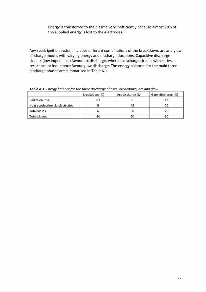
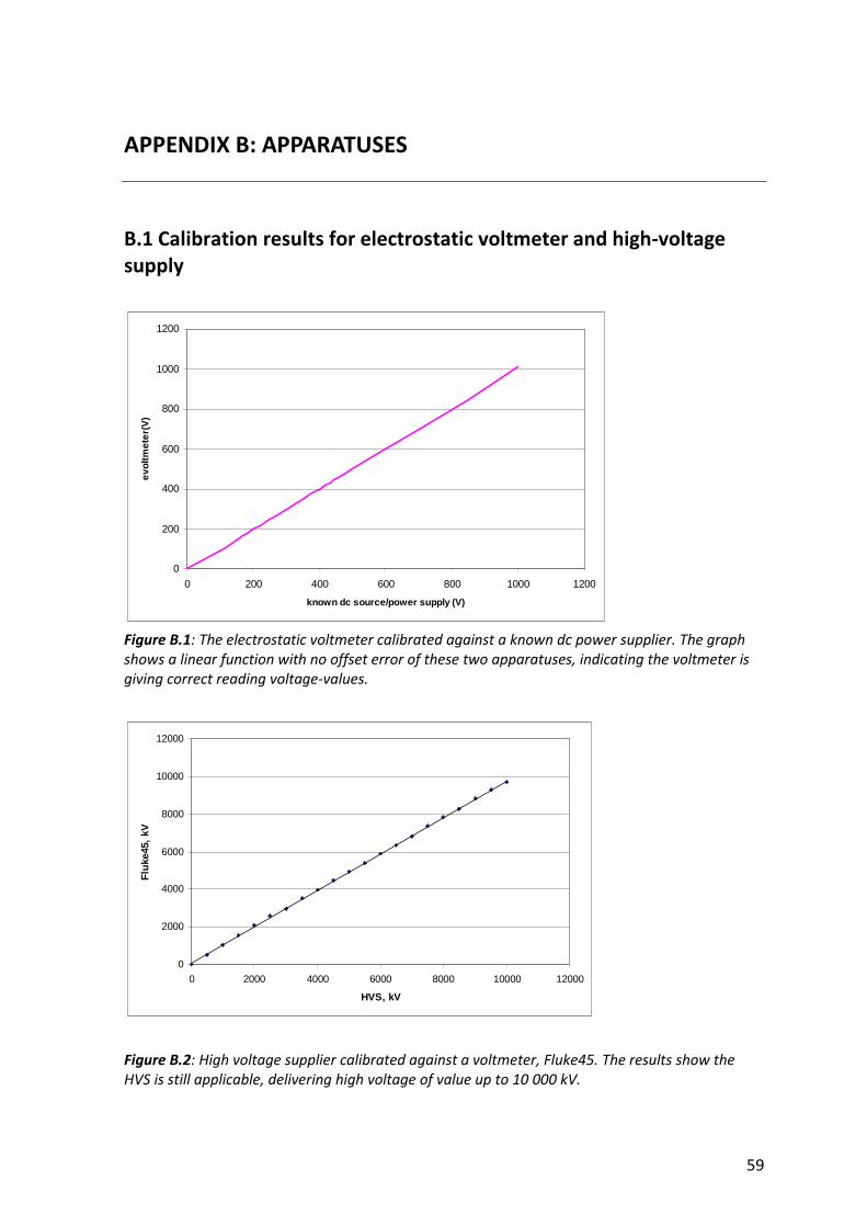
B.1 Calibration results for electrostatic voltmeter and high-voltage supply .................. 59
B.2 Gas mixing system for propane/air ........................................................................... 60
B.3 Servomex 1100A oxygen analyser............................................................................. 61
B.4 Servomex 1410, the gas analyser.............................................................................. 63
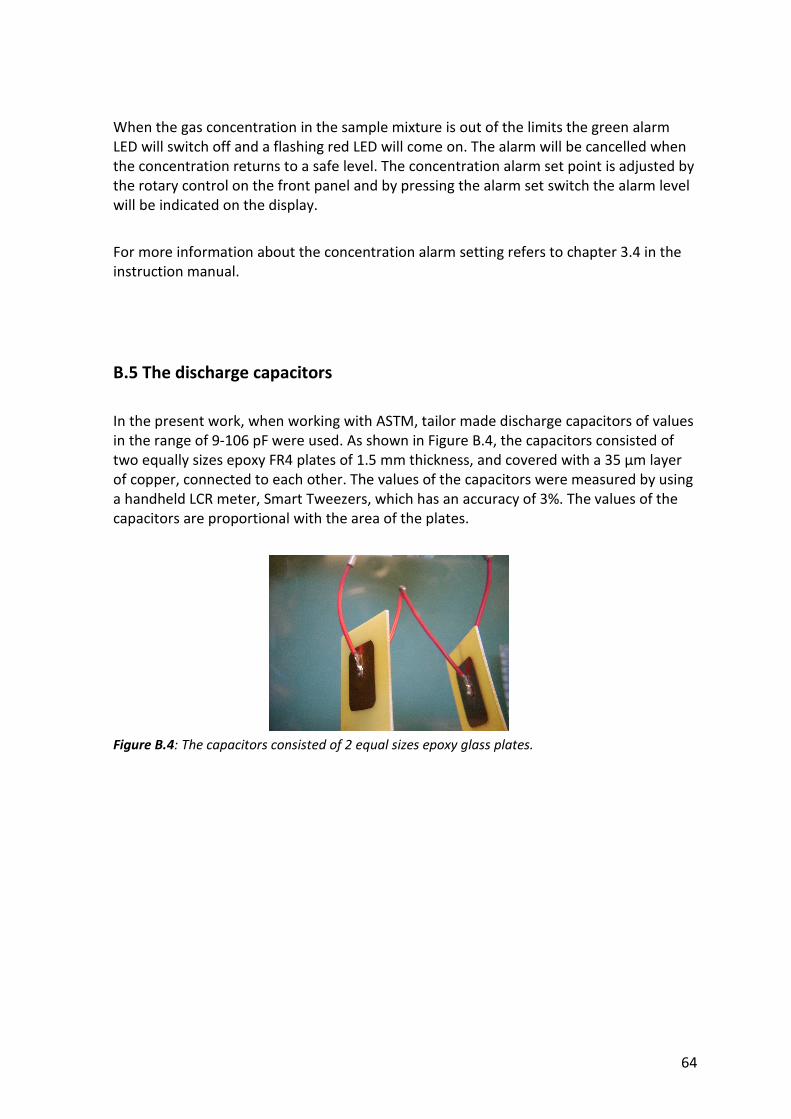
B.5 Photos of the apparatuses ........................................................................................ 65
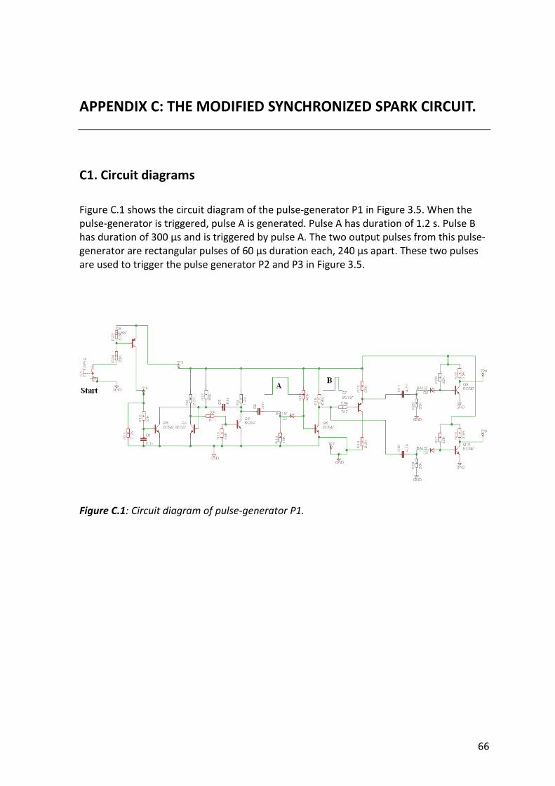
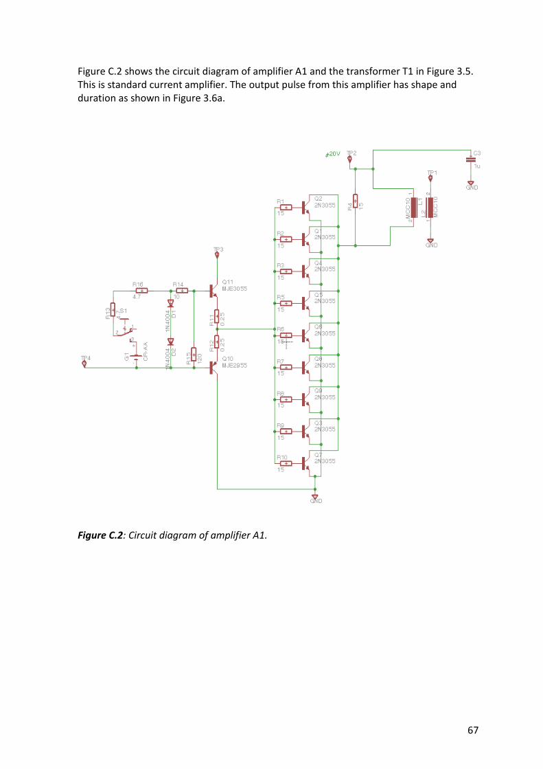
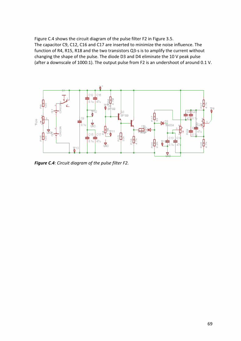
APPENDIX C: THE MODIFIED SYNCHRONIZED SPARK CIRCUIT............................................. 66
C1. Circuit diagrams......................................................................................................... 66
C2. Experimental results.................................................................................................. 72
Page 4
iii
ABSTRACT
This Master thesis describes an experimental study aimed at determining the minimum
ignition energy (MIE) of premixed propane/air mixtures. Two fundamentally different
circuits have been employed for creating the sparks in the experiments: a replica of the
American Society for Testing and Materials (ASTM) apparatus (ASTM, 2007) and an
improved version of the synchronized spark generator described by Randeberg et al.
(2006).
The explosion vessel was a 0.20 dm3 cylindrical plastic tube, equipped with two 1.6 mm
flat-ended tungsten electrodes. In the present work, the electrodes were flanged with
glass plates and the spark gap was set to 2.0 mm.
The principle of the capacitive spark circuit of ASTM was to charge an appropriate
capacitance connected across the spark gap through a large resistor (1012
Ω) by a high-
voltage power supply until the spark occurred. Different spark energies could be obtained
mainly by varying the value of the capacitance.
Premixed propane/air was used as test gas. About 220 tests were performed with the
ASTM circuit to find the boundary between ignition and no-ignition in propane/air
mixtures. The investigated propane concentrations were in the range 3.5 to 8.0 vol. %. By
following the approach of Moorhouse et al. (1974), the MIE in the present work was
determined by drawing the highest possible boundary line through all the experimental
points that had no ignition points below it. This resulted in a minimum ignition energy of
0.48 mJ at a propane concentration of 5.2 vol. %. This is twice the value reported by Lewis
and von Elbe (1961), but in very good agreement with the result obtained by Moorhouse
et al..
The quenching effect of the 2.0 mm spark gap for propane/air mixtures of less than 4.0
vol. % was confirmed. However, the present results do not indicate that 2.0 mm is the
quenching distance for any specific concentration on the fuel rich side in the investigated
concentration range (3.5-8.0 vol. %). According to the data reported by Lewis and von
Elbe, a flanged spark gap of 2.0 mm should correspond to the quenching distance for a
propane/air concentration of about 6.0 vol. % on the fuel rich side.
The probability of ignition for propane/air mixtures of 5.2 and 5.5 vol. % were also studied
by varying the spark energy levels in the range 0.40 to 0.75 mJ for both concentrations.
Based on the classical U-shaped curve by Lewis and von Elbe (1961), presenting MIE as
function of propane concentration, it was expected that a mixture of 5.2 vol. % propane
in air would be more ignitable than a mixture of 5.5 vol. %. However, the present results
do not show any significant difference in the ignitability for the two concentrations. By
applying a statistical model to the data at each of the two concentrations, MIE for 1%
probability of ignition were calculated. They were both significantly higher than the Lewis
and von Elbe value of 0.25 mJ.
Page 5
iv
Randeberg et al. (2006) described a spark generator for producing synchronized
capacitive spark discharges of low energy, down to below 0.1 mJ. However, Eckhoff et al.
(2008) re-examined the discharge circuit of Randeberg et al., and concluded that, due to
the hidden subtle energy supply, the real spark energies in the experiments were
significantly larger than those quoted in the published paper. The additional energy in the
discharge was of the order of 1 mJ.
With the aim to minimize the additional energy, an improved version of the Randeberg et
al. (2006) spark generator was constructed, which reduced the additional energy input to
the order of 0.25 mJ.
However, this required a considerable effort and time. Hence, due to lack of time, the
experimental work for the determination of MIE as a function of propane/air
concentration was not completed. Therefore, it was decided to perform a series of tests
at one propane concentration only. The propane concentration of 5.2 vol. % was selected,
because this was the concentration given the lowest ignition energy in the ASTM spark
generator tests. About 50 tests were performed to determine the highest total spark
energy below which there were no ignitions. A firm conclusion cannot be drawn due to
the limited number of tests. However, the experimental data indicate a MIE value for 5.2
vol. % propane/air mixtures of 0.36 mJ, which is lower then the MIE value obtained by
using the ASTM method (0.48 mJ).
It was observed that the shape and amplitude of the tail/undershoot of the spark pulses
varied from test to test, indicating that the synchronized-spark generator requires further
improvement.
Page 6
v
ACKNOWLEDGEMENTS
This study was conducted at the Department of Physics and Technology, University of
Bergen, Norway. As in many other experimental studies, the process of building and
commissioning the test system was quite a challenge and proved to be more time
consuming than expected. Personally I found the last year of the Master’s program to be
tough, but also educative.
First of all I would like to thank my supervisor, Professor Rolf K. Eckhoff for his invaluable
guidance, understanding and support. His devotion for knowledge has been truly inspiring.
My special thanks goes also to senior engineer, Werner Olsen, my second supervisor,
without whom it would not have been possible to construct the new spark generator.
Through the past year I have learned a lot from him.
It has been a hard year, and I would like to thank my family and friends for their love and
support. My classmates have been helpful throughout the project. I will also thank Martin
Hansen from the Department of Chemistry, Professor Ivar Heuch from the Department of
Mathematics, and senior engineer Kåre Slettebakken and his staff in the Mechanical
Workshop at the Department of Physics and Technology for their contributions.
I would like to thank Trygve Skjold of GexCon AS for lending me some of the reading
materials. Last but not least I wish to express my gratitude to the ELSTATIK foundation in
Germany for sponsoring this project and associate Professor Bjørn J. Arntzen for his tips
and advices throughout the project.
Page 7
1
CHAPTER 1: INTRODUCTION
1.1 GENERAL OVERVIEW
1.1.1 Background
A key concern in process safety is to prevent explosions and mitigate their effects. Over
the years, safety technology in the industry has improved continuously. These days, most
industries in “the industrialized world” are operating on a reasonably high safety level.
Although explosions in the process industries still happen. The concerns nowadays are
not just on human life and material losses, but also on the potential impact on the
environment. Therefore, process safety continuous to be important in the industry
throughout the world.
An explosion is often identified by a loud noise, or “bang” resulting from the sudden
release of energy. A more precise definition in the present context (Eckhoff, 2005) is to
define an explosion as an exothermal chemical process that, when occurring at constant
volume, gives rise to a sudden and significant pressure rise. Accidental explosions in the
process industries include gas, spray/mist and dust explosions. These three categories of
chemical explosions have similar ignition and combustion properties.
In the oil and gas industries, most gas explosions happen when combustible gas from
accidental releases, mixes with air in the atmosphere and generates an explosive cloud. If
the fuel/air ratio in the cloud is within the flammability limits, and there is a presence of
an ignition source, an explosion will occur.
1.1.2 Ignition sources
Explosive gas mixtures can be ignited by many types of ignition sources or sources of
energy that initiates combustion (Babrauskas, 2003). (Eckhoff, 2005) lists the following 8
types of ignition sources:
- open flames
- glowing or smouldering materials
- hot solid surfaces
- burning metal particles and “thermite” flashes from impacts, grinding, etc
- electrical and electrostatic sparks, arcs, and other forms of discharges
Page 8
2
- jets of hot combustion gases
- adiabatic compression
- light radiation
Extensive reviews of the standard test methods and published experimental studies
concerning the determination of critical ignition parameters, such as Tmin (minimum
ignition temperature) and MIE (minimum ignition energy), for gaseous fuel-air mixtures
can be found in the books of Babrauskas (2003) and Magison (1998). These parameters
can vary substantially with the actual ignition source characteristics, the dynamics,
pressure and temperature of the gas mixture.
1.1.3 Minimum ignition energy concept
The term minimum ignition energy (MIE) is an important parameter in explosion hazard
evaluation. It refers to the smallest amount of energy that an electric spark discharge
must have to cause an ignition of a given gas mixture at given conditions.
For the last century, many experimental studies have been done to investigate the true
values of the minimum ignition energy for different hydrocarbon fuels. MIE values
depend not only on the composition of the mixture, but also on the method of the spark
generation and properties of the electric circuit. Parameters such as gas concentration,
pressure, temperature, flow characteristics, spark gap length, and discharge duration also
influence the MIE.
1.1.4 MIE theories
There are two basic theories of ignition process by electric sparks: The electrical model
considers transport of chemical energy by the internal diffusion of reactants and reaction
products while the thermal model considers the transport of the thermal energy i.e. heat.
Even while no complete ignition theory was available, Strid (1973) concluded that the
hypothesis of thermal ignition seemed to be supported by the experimental MIE
determination. A recent overview of ignition theories is given by Babrauskas (2003).
According to the thermal theory of electric spark ignition of Lewis and von Elbe (1961),
the spark establishes instantly a small volume of hot gas immediately after the discharge.
At first the temperature within this flame kernel increases rapidly, but as the ignition
volume grows in size, the temperature decreases due to the flow of heat to the ambient
unburned gas. In the adjacent layer of ambient gas the temperature rises and induces
chemical reactions, so that a combustion wave is formed and propagates outwards. At
the time that the temperature within the flame kernel has decreased to the order of
normal flame temperature, the diameter of the flame kernel must have grown to a
certain size for self-sustained combustion, i.e. ignition, to be established. The flame
kernel has more or less a spherical shape. If the size is too small, the heat loss to the
Page 9
3
unburned gas continuously exceeds the heat gain by chemical reaction, so that the
reaction will gradually cease, leading to the extinction of the combustion wave (after only
a small amount of gas around the original spark has burned). The minimum ignition
energy is the energy required to establish the flame kernel of the minimum critical size
for subsequent self-sustained flame propagation. Figure 1.1 gives an overview of the
energy balance for electric spark discharge based on the thermal theory.
The electrical theory of electrical spark ignition supposes that the electrical discharge
activates the chemical reaction by producing free radicals/ions in the discharge zone,
which diffuse into the surrounding gas and initiate a self-propagating combustion chain.
Therefore the ignition conditions of the mixture are dependent on the concentration of
the reactive particles.
Figure 1.1: Energy balance of an electric spark discharge based on the heat (thermal) theory. From
Eckhoff (1970).
In practice, accidental electrical spark discharges are usually of capacitive nature i.e.
electrostatic discharges. Babrauskas (2003) divides discharges which have caused
accidental ignitions into 6 different categories; corona, brush, powder heap, spark,
propagating brush and lightning-like discharge. In the present work, only spark discharges
are used as ignition source. Appendix A.1 provides more detailed definitions of these
terms.
1.1.5 MIE in relation to incendivity of electrostatic discharges
The commonly published minimum ignition energies for most alkanes in air at normal
temperature and pressure are of the order of 0.25 mJ. According to Lüttgens and Glor
(1989), corona discharges have an equivalent energy of less than 0.02 mJ. This indicates
that corona discharges may only be effective ignition sources for the easiest ignitable
gases like hydrogen, acetylene and CS2. However, according to Babrauskas (2003), in
reality, it is unlikely that a corona discharge will ignite flammable atmospheres at all due
to its diffuse nature.
Page 10
4
Brush discharges on the other hand can generate equivalent spark energies of up to 3 mJ,
and the very energetic propagating brush discharges can generate up to 105 mJ. Hence,
these two discharge types are effective ignition sources for most explosive gas mixtures.
Crowl (2003) emphasised that it is also important to remember that the MIE of 0.25 mJ is
a very low energy, e.g. corresponding to the kinetic energy of a small coin as it impacts a
surface after being dropped from a height of only a few millimetres. An electrostatic
discharge that can be felt by a person has an energy of at least 20 mJ, i.e. about two
orders of magnitude greater than 0.25 mJ. Therefore, the elimination of ignition sources
should not be relied on as the sole defence against fires and explosions of gases and
vapours.
1.1.6 Spark discharge features that may influence spark incendivity
The establishment of a self-sustained flame front in the combustible gas mixture is
strongly influenced by the discharge mode and the geometry of the plasma volume,
generated by the spark discharge. The total energy involved plays only a minor role. Maly
and Vogel (1978) divided the spark discharge process in three main phases: breakdown,
arc and glow phases. Any spark ignition system includes a different combination of these
three discharge modes, with varying energy content and durations depending on the
discharge circuit. Figure 1.2 shows both gap voltage and current vary as functions of time
during a spark discharge.
With a very short spark durations of the order of 10-9
s (1 ns) more than 80% of the
energy is transformed into plasma during the breakdown phase. The arc and glow phases
last much longer and their energy transfer efficiencies are much less. A more detailed
description of the characteristics of the three discharge phases are given in Appendix A.2.
Figure1.2: Schematic diagram of voltage and current vs. time in a spark discharge of a typical
spark ignition system. The six discharge phases are: i) pre-discharge, ii) breakdown, iii)
breakdown/arc transition, iv) arc, v) arc/glow transition, and vi) glow. From Maly and Vogel (1978)
Page 11
5
1.1.7 “Break” sparks and “jump” sparks
It is useful to distinguish between two types of electric sparks, viz. break spark and jump
spark.
Break sparks occur when a circuit carrying an electric current is broken. The character of
the break spark depends on the relationship between the inductance and the ohmic
resistance in the circuit. The spark energy can usually be calculated by the formula
E = ½ Li2, where L is the inductance and i the current.
Jump sparks are caused by the release of electrical energy stored on a capacitor across a
spark gap. The spark energy is calculated by the formula E = ½ CU2 where C is the
capacitance and U is the voltage. The capacitor energy is in electrostatic form and the
spark occurs when the voltage of the spark gap reaches the breakdown voltage.
1.2 OBJECTIVE OF THE PRESENT WORK
The work described in this thesis consists of two main phases:
Phase 1
a) Construction of a copy of the ASTM standard apparatus (E 582 - 07) for
determination of MIE for explosive premixed gases.
b) Determination of MIE for propane/air as a function of vol. % propane in the
mixture, using the standard ASTM apparatus.
c) Analysis of results by comparing with available published data.
Phase 2
a) Construction of an improved version of the new electric spark generator for
producing synchronized capacitive spark discharges of low energies, as indicated
by Eckhoff et al. (2008). The aim of the improvement is to minimize the additional
energy contribution to the effective spark energy due to the minute stray current
following the main current pulse from the discharge capacitor.
b) Determination of MIE for propane/air as a function of vol. % propane in the
mixture, using the new, improved synchronized-spark generator.
c) Comparison of results from 1b)/c) and 2b).
Page 12
6
CHAPTER 2: REVIEW OF PREVIOUS WORKS
2.1 MIE AND QUENCHING DISTANCE
The quenching distance, QD, is the smallest distance between two surfaces that permits
laminar flame propagation in a homogeneous quiescent explosive gas mixture to take
place in the space between them. In relation to electric spark ignition, the term
quenching distance refers mostly to the minimum distance between the electrodes which
allows optimal ignition, with a minimal energy loss to the electrodes.
The QD is a very important parameter for MIE determination. It does not only depend on
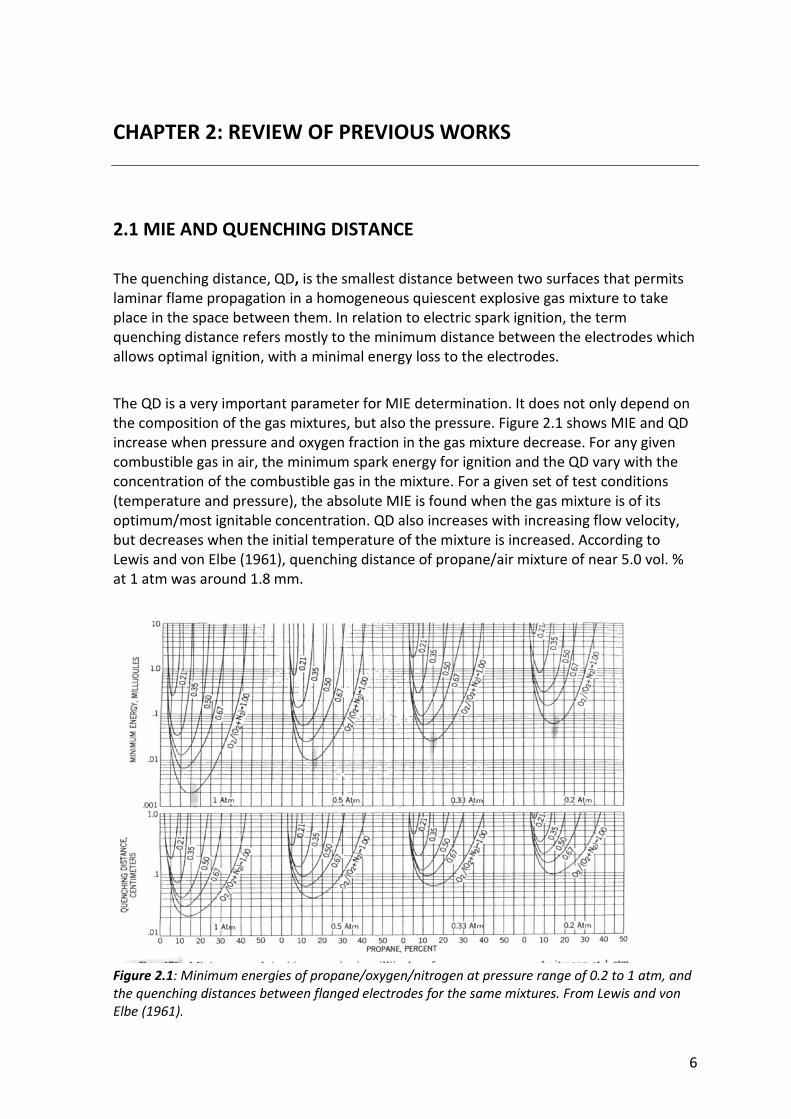
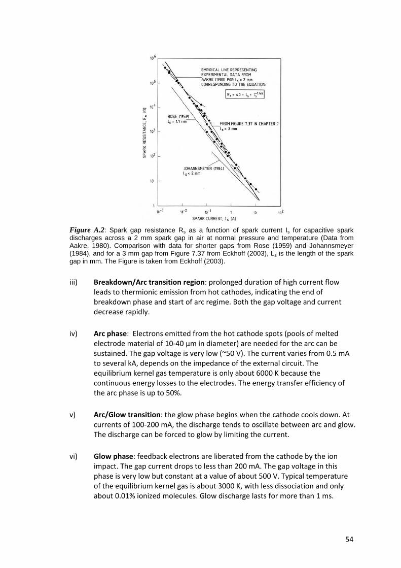
the composition of the gas mixtures, but also the pressure. Figure 2.1 shows MIE and QD
increase when pressure and oxygen fraction in the gas mixture decrease. For any given
combustible gas in air, the minimum spark energy for ignition and the QD vary with the
concentration of the combustible gas in the mixture. For a given set of test conditions
(temperature and pressure), the absolute MIE is found when the gas mixture is of its
optimum/most ignitable concentration. QD also increases with increasing flow velocity,
but decreases when the initial temperature of the mixture is increased. According to
Lewis and von Elbe (1961), quenching distance of propane/air mixture of near 5.0 vol. %
at 1 atm was around 1.8 mm.
Figure 2.1: Minimum energies of propane/oxygen/nitrogen at pressure range of 0.2 to 1 atm, and
the quenching distances between flanged electrodes for the same mixtures. From Lewis and von
Elbe (1961).
Page 13
7
As pointed out by Babrauskas (2003), the most effective spark gap length for ignition is
slightly greater than the QD. If the electrodes are placed closer together than the QD,
they will act as a heat sink and remove heat from the developing flame kernel, and
therefore the required ignition energy will increase. Figure 2.2 indicates that the size and
shape of electrodes do not significantly affect the values of MIE at electrode distances
larger than the QD. But for smaller distances, the influence of these factors are significant.
Flanged electrode is an extreme situation as indicated by the sharp and quite dramatic
increase of MIE as soon as the spark gap becomes less than the QD. This is due to the
cooling effect of the flanges, which prevents a laminar gas flame from propagating
outwards from the spark between the flanges.
Figure 2.2: Minimum ignition energies for free and glass-flanged electrode tips as a function of
electrode distance. Stoichiometric mixture of natural gas (about 83% CH4 + 17% C2H6) and air at 1
atm pressure was used. From Lewis and von Elbe (1961)
As mentioned earlier, the minimum spark energy for ignition is a function of the gas
concentration of the mixture. Figure 2.3 shows the minimum ignition energies for
different hydrocarbon fuels as U-shaped functions of the gas concentration. The
minimum ignition energy, MIE, is defined as the minimum value of the U-shaped function.
It should be noticed that the fuel-air equivalence ratio Φ at which the MIE occurs
increases with increasing carbon number, exhibited a steady shift toward fuel rich
conditions. Due to the higher diffusivities, MIE of molecules lighter than air (for example
like hydrogen and methane) occurs in lean mixture, i.e. when the fuel equivalence ratio,
Φ < 1. Figure 2.3 shows MIE value of methane is slightly higher than those of the higher
alkanes.
Page 14
8
Figure 2.3: Minimum capacitive ignition energies of various gaseous alkanes/air mixtures as a
function of the volumetric ratio of fuel and air. From Eckhoff (2005)
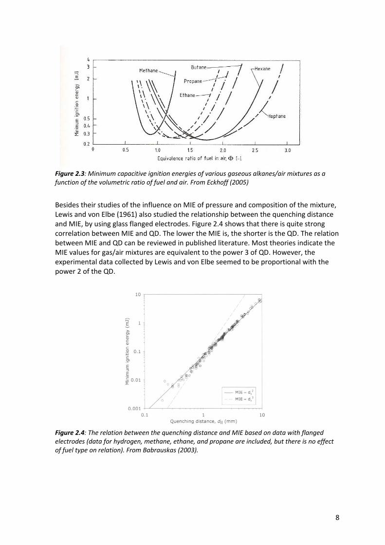
Besides their studies of the influence on MIE of pressure and composition of the mixture,
Lewis and von Elbe (1961) also studied the relationship between the quenching distance
and MIE, by using glass flanged electrodes. Figure 2.4 shows that there is quite strong
correlation between MIE and QD. The lower the MIE is, the shorter is the QD. The relation
between MIE and QD can be reviewed in published literature. Most theories indicate the
MIE values for gas/air mixtures are equivalent to the power 3 of QD. However, the
experimental data collected by Lewis and von Elbe seemed to be proportional with the
power 2 of the QD.
Figure 2.4: The relation between the quenching distance and MIE based on data with flanged
electrodes (data for hydrogen, methane, ethane, and propane are included, but there is no effect
of fuel type on relation). From Babrauskas (2003).
Page 15
9
2.2 THE STUDY OF LEWIS AND VON ELBE
2.2.1 Overview
The classical MIE data reported by Lewis and von Elbe (1961) are often referred to as
absolute standards. According to the results of their experimental work, MIE of
propane/air mixture was 0.26 mJ at ambient conditions. The optimal concentration for
ignition was about 5.3 % vol.
2.2.2 Test apparatus
The original apparatus was first described by Guest (1944) and later modified by Blanc,
Guest, von Elbe and Lewis (1947). The stainless steel test bomb had an inner diameter of
127 mm and the spark gap was located in the centre. The gap length could be adjusted by
a built-in micrometer. 1.6 mm diameter pointed and flanged electrodes were used to
determine MIE for different conditions. Glass flanges were mostly used because metal
flanges are electrically conductive and had a tendency to cause ignition even within the
quenching distance.
However, due to the electrical conductivity of the glass surface, Lewis and von Elbe did
observe irregular discharges, particularly corona discharges, during their experiments
even with glass flanges. To eliminate this source of error, the glass flanges could be
coated with paraffin wax. But according to Strid (1973), Litchfield (1967) pointed out that
the flanges should in fact be slightly conductive in order to equalize the electric potential.
2.2.3 Electrical spark-generation circuits
According to Kravchenko (1984), the spark generated by the circuit of Lewis and von Elbe
had durations down to 1µs, indicating that their spark discharges were arc discharges. All
tests conditions were controlled to eliminate energy losses. The energy storage
capacitance could be varied over the wide range from 1 pF to 5000 pF, using two different
apparatuses.
Electric circuit for capacitances > 100 pF
The circuit is as shown in Figure 2.5. High voltage was supplied through protective resistor
to terminal “a” from a power unit. The rotating charger, consisting of two insulated metal
Page 16
10
balls, transferred the high voltage gradually to the discharge capacitor which connected
to the electrodes mounted to explosion vessel. In this way, the transferring charge rate
could be controlled by varying the angular velocity of the rotating charger. Due to high
values of the capacitors, the delay time, time before the spark occurred was often long.
This lag of time could be reduced by placing radium capsules of various strengths into the
test bomb. But in later work this was found potentially troublesome due to the caused
slow leakage of electricity from the charged electrode before the breakdown.
Electric circuit with capacitances < 100 pF
In later work, the rotary charger was replaced by a Bakelite rod resistor of order of 1011
Ω.
This high resistor rod had the same function as the rotary charger, and that was
permitting a slow transfer of charge from the power unit to the spark circuit. The
capacitors and the static voltmeter were now connected in parallel and used as a
reservoir of known voltage, as shown in Figure 2.6. From this reservoir the voltage was
charged to a desired potential, then isolated from the power unit and electricity was
delivered to the test bomb through the Bakelite rod. The capacitance of the spark circuit
could be adjusted down to 1 pF by means of the small extension capacitors and other
devices.
Figure 2.5: Scheme of apparatus for
determining minimum ignition energies for
electric-spark ignition. From Lewis and von Elbe
(1961)
Figure 2.6: Apparatus arranged for spark circuit
of very low capacitance .From Lewis and von
Elbe (1961)
Page 17
11
2.2.4 Test method and statistical MIE criterion
After the desired spark gap was set, the explosion vessel was filled with a gas mixture of
the desired composition. The electrode and the capacitor system was slowly charged and
the voltage, U, at which the spark occurred was recorded. If the mixture did not ignite,
the capacitance was increased by trial and error until the critical capacitance, C, for
ignition was found. The ignition energy was calculated by the formula E = ½ CU2, where U
was the voltage just before spark discharge and C the energy storage capacitance.
It has not been possible to trace the statistical method used by Levis and Elbe for deriving
MIE from the experimental data, but according to Moorhouse et al. (1974), their criterion
was an ignition probability of only 1 %.
2.3 THE ASTM METHOD
2.3.1 Overview
The standard test method for MIE and QD in gaseous mixtures from ASTM (2007) is based
on the Bureau of Mines/Lewis and von Elbe method. The method is applied to mixtures of
specified fuels (gases and vapours of liquids) with air. The mixing ratio is varied from the
most easily ignitable mixture to mixtures near to the flammable limit compositions. The
breakdown voltage of the spark gap follows Paschen’s law, which means that it depends
on the gas mixture pressure, spark gap distance and the gas mixture composition.
With this standard test method, the expected accuracy is ± 10% in minimum ignition
energy for MIE and ± 2% for QD. For mixture compositions near the flammable limits, the
MIE increased rapidly as the flammable limits are approached and hence the standard
deviation of ±10% does not apply here.
2.3.2 Test apparatus
The recommended reaction chamber is 1 dm3 spherical stainless steel vessel of inner
diameter (125mm). The 1.6 mm diameter metal electrodes shall be flanged with glass
plates. The glass flanges should have a diameter of 5 to 10 times the electrode gap and a
thickness of 2.38 - 3.18 mm.
For maximum testing flexibility, a DC power supply that can deliver 1-30 kV is
recommended.
Page 18
12
2.3.3 Electrical spark generation circuit
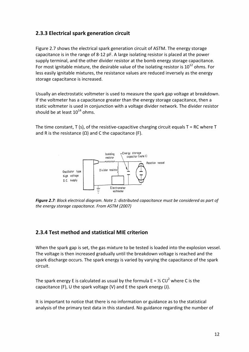
Figure 2.7 shows the electrical spark generation circuit of ASTM. The energy storage
capacitance is in the range of 8-12 pF. A large isolating resistor is placed at the power
supply terminal, and the other divider resistor at the bomb energy storage capacitance.
For most ignitable mixture, the desirable value of the isolating resistor is 1012
ohms. For
less easily ignitable mixtures, the resistance values are reduced inversely as the energy
storage capacitance is increased.
Usually an electrostatic voltmeter is used to measure the spark gap voltage at breakdown.
If the voltmeter has a capacitance greater than the energy storage capacitance, then a
static voltmeter is used in conjunction with a voltage divider network. The divider resistor
should be at least 1014
ohms.
The time constant, T (s), of the resistive-capacitive charging circuit equals T = RC where T
and R is the resistance (Ω) and C the capacitance (F).
Figure 2.7: Block electrical diagram. Note 1: distributed capacitance must be considered as part of
the energy storage capacitance. From ASTM (2007)
2.3.4 Test method and statistical MIE criterion
When the spark gap is set, the gas mixture to be tested is loaded into the explosion vessel.
The voltage is then increased gradually until the breakdown voltage is reached and the
spark discharge occurs. The spark energy is varied by varying the capacitance of the spark
circuit.
The spark energy E is calculated as usual by the formula E = ½ CU2 where C is the
capacitance (F), U the spark voltage (V) and E the spark energy (J).
It is important to notice that there is no information or guidance as to the statistical
analysis of the primary test data in this standard. No guidance regarding the number of
Page 19
13
tests to be done at each spark energy level and the probability of ignition to be associated
with MIE is given.
2.4 THE STUDY OF MOORHOUSE ET AL.
2.4.1 Overview
Moorhouse et al. (1974) determined the MIEs for C1 to C7 hydrocarbon/air mixtures. They
also investigated the dependence of MIE on initial pressure and temperature. Their
conclusion seemed to support the results reported by others. They found that MIE
decreased with increasing temperature and pressure of the unburned gas mixture.
It is interesting to note that the MIE values reported by Moorhouse et al. were generally
significantly higher than those reported by Lewis and von Elbe (1961). For example, the
reported MIE of propane/air at ambient conditions and at optimal propane concentration
of 5.3 vol. % was 0.46 mJ, whereas the value reported by Lewis and von Elbe (1961) was
only 0.25 mJ.
2.4.2 Test apparatus
The stainless steel test vessel was a cylindrical with a diameter of 50 mm and length of
200 mm. The vessel was fitted with diametrically opposite 1.0 mm diameter tungsten
electrodes. One of the electrodes could be moved to vary the electrode spacing and its
position measured by a dial micrometer.
2.4.3 Electrical spark generation circuit
Based on the technique of Cheng (1967), the sparks of Moorhouse et al. (1974) were
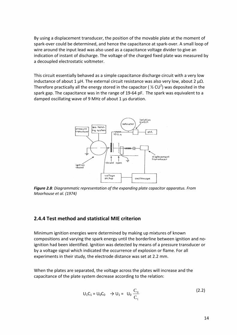
generated by means of the variable air capacitor device as illustrated in Figure 2.8. The
capacitor consisted of two parallel plates, each 100x200 mm. The fixed plate was
connected to the high-voltage electrode in the explosion vessel and the movable plate
connected to the other earthed electrode. When the fixed plate had been charged from a
high voltage source, the spring loaded movable plate was released and opened from its
closest separation to the fixed plate (about 1 mm). The distance between the plates was
increased rapidly. This caused a decrease of the capacitance and a corresponding increase
of the voltage across the capacitor, and hence across the spark gap. A discharge between
the electrodes occurred when the plate separation had caused a sufficient rise in voltage.
Page 20
14
By using a displacement transducer, the position of the movable plate at the moment of
spark-over could be determined, and hence the capacitance at spark-over. A small loop of
wire around the input lead was also used as a capacitance voltage divider to give an
indication of instant of discharge. The voltage of the charged fixed plate was measured by
a decoupled electrostatic voltmeter.
This circuit essentially behaved as a simple capacitance discharge circuit with a very low
inductance of about 1 μH. The external circuit resistance was also very low, about 2 μΩ.
Therefore practically all the energy stored in the capacitor ( ½ CU2) was deposited in the
spark gap. The capacitance was in the range of 19-64 pF. The spark was equivalent to a
damped oscillating wave of 9 MHz of about 1 µs duration.
Figure 2.8: Diagrammatic representation of the expanding plate capacitor apparatus. From
Moorhouse et al. (1974)
2.4.4 Test method and statistical MIE criterion
Minimum ignition energies were determined by making up mixtures of known
compositions and varying the spark energy until the borderline between ignition and no-
ignition had been identified. Ignition was detected by means of a pressure transducer or
by a voltage signal which indicated the occurrence of explosion or flame. For all
experiments in their study, the electrode distance was set at 2.2 mm.
When the plates are separated, the voltage across the plates will increase and the
capacitance of the plate system decrease according to the relation:
U1C1 = U0C0 → U1 = U0 1
0
C
C
(2.2)
Page 21
15
Where U0 and C0 are the voltage and capacitance before plate separation, and U1 and C1
the voltage and capacitance at spark-over. C1 was determined by the measurement of the
plate distance at spark-over.
The energy in the spark is:
E = ½ C1U12 (2.3)
By inserting equation 2.2 in 2.3, one gets:
E = U0 1
20
C2
C
(2.4)
The spark energy E in this study was calculated by using equation 2.4
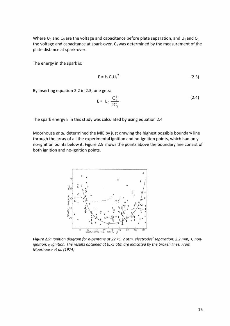
Moorhouse et al. determined the MIE by just drawing the highest possible boundary line
through the array of all the experimental ignition and no-ignition points, which had only
no-ignition points below it. Figure 2.9 shows the points above the boundary line consist of
both ignition and no-ignition points.
Figure 2.9: Ignition diagram for n-pentane at 22 ºC, 2 atm, electrodes’ separation: 2.2 mm; •, non-
ignition; o, ignition. The results obtained at 0.75 atm are indicated by the broken lines. From
Moorhouse et al. (1974)
Page 22
16
2.5 THE SYNCHRONIZED CAPACITIVE SPARK SYSTEM OF RANDEBERG.
2.5.1 Overview
In the circuit developed by Randeberg et al. (2006), a high voltage pulse was used for
charging the capacitor instead of using a static high-voltage power supply. In this way, the
moment of spark discharge could be determined precisely, which allowed synchronization
with e.g. transient dust cloud generation. It was claimed that low-energy electric sparks in
the range down to 0.03 mJ could be generated by using pointed electrodes, a spark gap of
1-2 mm and capacitance of a few pF. The main current pulse of sparks generated with this
circuit were breakdown discharges of very short durations of below 100 ns.
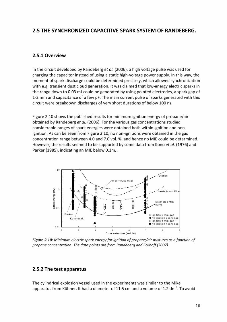
Figure 2.10 shows the published results for minimum ignition energy of propane/air
obtained by Randeberg et al. (2006). For the various gas concentrations studied
considerable ranges of spark energies were obtained both within ignition and non-
ignition. As can be seen from Figure 2.10, no non-ignitions were obtained in the gas
concentration range between 4.0 and 7.0 vol. %, and hence no MIE could be determined.
However, the results seemed to be supported by some data from Kono et al. (1976) and
Parker (1985), indicating an MIE below 0.1mJ.
0.01
0.1
1
10
2 3 4 5 6 7 8 9
Concentration (vol. %)
Sp
ark
ener
gy
(mJ)
Ignition 2 m m gapNo ignition 2 m m gapIgnition 4 m m gapNo ignition 4 m m gap
Lewis & von E lbe
D ietlen
Parker
Kono et a l.
Estim ated M IE curve
Moorhouse et a l.
Figure 2.10: Minimum electric spark energy for ignition of propane/air mixtures as a function of
propane concentration. The data points are from Randeberg and Eckhoff (2007).
2.5.2 The test apparatus
The cylindrical explosion vessel used in the experiments was similar to the Mike
apparatus from Kühner. It had a diameter of 11.5 cm and a volume of 1.2 dm3. To avoid
Page 23
17
corona discharge prior to breakdown, the 2.0 mm diameter tungsten electrodes were
rounded off to an angle of approximately 60°. The electrode gap widths were in the range
from 1.0 mm to 6.0 mm.
With the aim to reduce the noise influence on the measuring probes, a shield with an
integrated system for voltage and current measurement was placed around the
combustion vessel. As can be seen in Figure 2.11, this measurement system was also
integrated in the circuit.
2.5.3 Electrical spark generation circuit
A primary capacitor of 1 µF was charged to a voltage of about 300 V. By triggering the
thyristor, this capacitor would be discharged into the primary coil of a high-voltage
transformer and a pulse of about 15 kV was generated in the secondary windings of the
transformer. The high-voltage pulse had a rise time of about 0.7 ms and was supplied to
the discharge capacitor through a charging resistor. This produced a corresponding
voltage build-up on the discharge capacitor. When the breakdown voltage of the
electrode gap was reached, the energy in the discharge capacitor was delivered to the
spark gap.
To avoid recharging of the discharge capacitor during the spark discharge, the time
constant RC (where R was the charging resistance and C the discharge capacitance) had to
be at least 1 µs. Typical values of R were then between 100 kΩ and 1 MΩ, depending on
the size of the discharge capacitor. The spark discharge times were less than 100 ns.
The schematic layout of the spark discharge circuit is shown in Figure 2.11
Randeberg assumed that no further energy than that stored in the discharge capacitor
was delivered to the spark gap. As discussed in 2.5.5, this assumption as not valid. In the
present study, an improved version of the Randeberg et al. generator was developed and
repeated ignition tests with propane/air were performed.
Page 24
18
5
320 VChargingresistor
Oscilloscope
HV transformer
Thyristor
5 5
5
HV probe
Probe 1
Spark gap
Trigger pulse
3 pF
Dischargecapacitor
Primarycapacitor
1 uF
Measurementresistors
SymmetryresistorsCylindric shield
around combustionchamber
Probe 2
Figure 2.11: Schematic layout of the spark discharge circuit and the integrated spark energy
measurement system.
2.5.4 Determination of spark energy
Ignition tests were performed in series of ten successive trials at each energy level. The
net spark energy in each trial, E, was calculated by the following equation:
E ∫= Ui dt - ∫ RMi2 dt (2.5)
Where U and i are the instantaneous spark voltage and current, measured across the
spark gap during the life time of the spark pulse. The second term is the energy lost to the
measurement resistors.
The spark voltage as a function of time was measured by using a high-voltage probe. This
probe had a capacitance of 3 pF and had to be taken into account for calculation of the
total capacitance involved in the discharge. The current was measured by two
independent probes to reduce the noise influence (which was pronounced for the low
spark energies).
Page 25
19
2.5.5 Further investigation about MIE of propane/air based on the work of
Randeberg
With the aim to reduce the additional energy supply to the spark after discharge of the
discharged capacitor, Eckhoff et al. (2008) modified the circuit of Randeberg et al. (2006).
They pointed out that the circuit did allow a small current of about 1/1000 of the peak
current of the first pulse to continue to flow through the spark gap, after the main pulse
from the discharge capacitor has ended. This current had a value of around 20-50 mA and
lasted up to 100 µs, which corresponded to a substantial additional amount of energy of
more than 1 mJ. The real spark energies in the experiments by Randeberg and Eckhoff
(2007) were much larger than those quoted in their paper. Therefore this recent
investigation did not support the earlier published results of MIE value for propane/air
below 0.1 mJ.
2.5 MIE STUDIES BY OTHER WORKERS
2.5.1 The study of Calcote et al.
Calcote et al. (1952) used almost the same apparatus and procedure as used by Lewis and
von Elbe (1947) to determine MIE of a large number of fuel types, employing
stoichiometric fuel/air mixture at a pressure of 1 atm. With this circuit, a known (3000 to
4000 pF) capacitance in parallel with the spark gap was charged through a high resistance
of value 109-10
12 Ω until a spark occurred. 4.9 mm stainless steel hemisphere electrodes
were used. With the aim to reduce the spark breakdown lag and ensuring a constant
breakdown voltage at given electrode distance, the electrodes were irradiated with
ultraviolet light.
The MIE results for most gases from their work were in good agreement with data of
Lewis and von Elbe. At stoichiometric concentration, the values for some gases, including
propane, were slightly lower than those reported by Lewis and von Elbe.
2.5.2 The studies of Kono et al.
Kono et al. (1976) investigated MIE of lean propane/air mixtures related to optimum
spark durations by using composite spark, consisting of a short capacitive discharge of 0.5
µs and an inductive discharge of much longer duration. The spark energy was therefore
calculated as a sum of the capacitance spark energy of the first short pulse and the
integrated power of the secondary inductive component. The electrodes used in their
Page 26
20
experiments were 30° half cone tungsten wire of 0.3 mm diameter, separated in a
distance nearly equal to the quenching distance of the mixture.
Their study showed that the minimum ignition energies varied greatly with spark duration
and had minimum values when the spark duration was at optimum. At durations above
and below the “optimum”, the ignition energies were increasing. According to Kono et al.
(1992), the MIE for short spark durations increased due to the heat loss to the unburned
gas stream that cooled the flame kernel and the energy was taken away by the shock
wave. For long spark durations, the flame kernel remained near the spark gap, so that the
heat loss from the flame kernel to the spark electrode increased with increasing spark
duration. Spark energy supplied after the critical size of the flame kernel was formed (a
few hundred μs) would not contribute to ignition process, but only increase the overall
ignition energy.
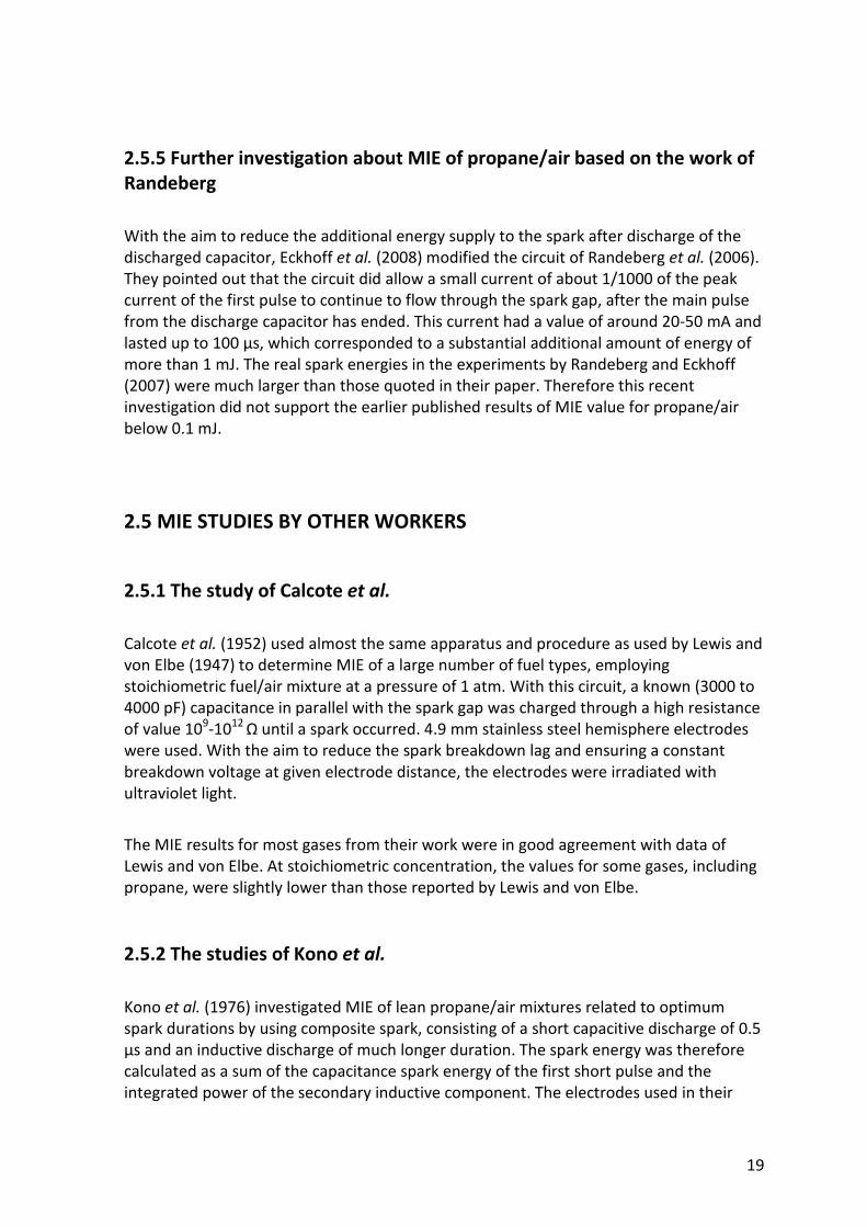
Figure 2.12 shows that the optimum spark duration for 3.0-3.5 vol. % propane/air mixture
is in the order of 50 μs. Even with 50% ignition frequency criterion, their lowest minimum
ignition energies were less than half of those which were reported by Lewis and von Elbe
(1961).
Figure 2.12: The effect of the spark duration on the minimum ignition energy for gap width nearly
equal to quenching distance. From Kono et al. (1976).
Knowledge about the flame kernel growth combined with MIE data provides a better
understanding of spark ignition. Kono et al. (1992) showed the influences of the
electrodes’ configuration and spark duration on the flame kernel structure. A short
summary of their work is given in appendix A.
2.5.3 The study of Parker
With the same aim as Kono et al. (1976), Parker (1985) also studied the influences of
discharge duration on the MIE for lean propane/air mixture. His pulse forming network
consisted of an arrangement of capacitors and inductors (“transmission line”). Parker
obtained well defined rectangular voltage and current pulses. The produced arc discharge
Page 27
21
had energies values of 0.1 to 20 mJ and durations in the range of 0.2 to 100 μs. The spark
energy was defined as the integral of power versus time across the spark gap. MIE was
defined as the spark energy giving an ignition probability of 10%. Parker used 0.5 mm
diameter electrodes in 3 different gap widths 2.0, 4.0 and 7.0 mm to study MIE in relation
to spark duration.
Parker found a strong dependence of MIE on the spark duration. MIE increased
significantly when spark duration was increased from 0.2 to 100 μs. With a 4.0 mm spark
gap, Parker found a MIE value of 0.3 mJ for 2.7 vol. % propane/air. This value cannot be
compared directly with Lewis and von Elbe’s data since their lowest experimental
concentration for propane/air was 3.0 vol. %.
2.5.4 MIE determination by using laser “sparks”
Generally, the MIE values obtained for propane/air by using laser sparks are higher than
data obtained with electrical sparks. Lee et al. (2001) used a laser spark ignition system to
study the MIE values of hydrocarbon fuels in air at a range of pressures and equivalence
ratios. For 5.0 vol. % propane/air, they found a MIE of about 0.6 mJ. This is considerably
higher than the value of 0.25 mJ, given by Lewis and von Elbe (1961), but not much higher
than 0.48 mJ found in the present investigation using the ASTM apparatus.
It’s important to emphasize that these differences between the MIE values are not just
due to the different measurement techniques, but also to different criterions of ignition
probability chosen to define MIE with.
2.7 STATISTICAL ANALYSIS OF SPARK IGNITION
Eckhoff (1970) pointed out that the term minimum ignition energy must be associated
with a certain ignition probability; otherwise it would be difficult to compare the obtained
values of MIE.
One question that arises is: What level of probability is most appropriate to use? A second
question is: How many trials are required to achieve a true or reliable ignition probability?
Ko et al. (1991) suggested that a probability of ignition of 50 % would be an appropriate
choice. In many experimental studies, ten trials at each energy level have been used. But
some workers emphasize that this sample size is too small to obtain sufficiently accurate
determination of the true probability. When discussing the theory of Bernoulli’s trials,
Eckhoff (1970) mentioned even sample sizes of 20 trials might not be large enough to give
the required accuracy in the determinations of the true probability of ignition.
Page 28
22
Due to the statistical nature of spark discharges, breakdown occurs at different
instantaneous voltages even when apparently identical test conditions are applied. The
representative value of breakdown voltage would be the calculated arithmetic mean:
U break (mean) = ∑n
1U break
(2.6)
Here n is the number of spark discharges and Ubreak the breakdown voltage. But this may
lead to an untrue value of minimum ignition energy because for achieving high accuracy
of the results, it often requires a large number of tests, n.
It is also reasonable to state that the ignition probability, P, of a given combustible
mixture increases with increasing spark energy. The probability of ignition P is denoted as
the ratio of the number of ignitions, m is the total number of spark discharges in the total
number of tests, n.
P = m/n (2.7)
Moffett et al. (2007) re-emphasized that there is no single threshold energy value, but a
distribution of the probability of ignition versus spark energy. They applied logistical
regression for binominal outcomes to analyze the results of spark energies near the
reported MIE, where the energy levels for ignition and no-ignition results overlap. The
result was S-curve with ignition probability as a function of spark energy, with 95%
confidence envelope is shown in Figure 2.13. Spark energy levels where only no-ignition
or ignition are obtained have ignition probabilities of 0 and 1 respectively. In the following,
E denotes MIE for a given probability P of ignition.
Based on the logistic regression model the probability of ignition, P(E), for a given spark
energy, E, can be calculated by the following equation:
P(E) = i10 Ee1
1β−β−+
(2.8)
Where β0 and β1 are coefficients estimated by maximizing the likelihood function.
With the known parameter, for a certain probability of ignition P(E), values of spark
energy, E, can be calculated by:
E = (ln)E(P1
)E(P
−- β0) / β1
(2.9)
Page 29
23
The disadvantage of equation 2.9 is E cannot be found when P(E) = 1.0, because the
natural logarithm of 0 would be negative infinity. However, the equation is applicable to
any value close to unity.
The upper confidence limit (UCL) and lower confidence limit (LCL) for the 95% confidence
interval for E can be estimated by:
LCLUCL = E ± zα/2 2
1112
0100 /)EE2( βσ+σ+σ (2.10)
Where σ00, σ01 are the variances and σ11 is the covariance of β0 and β1. α for 95%
confidence interval is 0.05 hence zα/2 is the z value from a standard normal distribution.
The covariance of β0 and β1, σ11 is the product of correlation factor, ρ and standard
deviations of β0 and β1.
Figure 2.13: Logistic probability distribution and 95% confidence envelope for Jet A spark ignition
data. The original data points are also plotted in the diagram. As in any binominal outcome model,
y=1 for a ”success”( in this case is ignition) and y=0 for a “no success”(no-ignition) for a given
spark energy. From Muffett et al. (2007).
Page 30
24
CHAPTER 3: METHODS AND APPARATUSES USED IN THE
PRESENT WORK
3.1 THE ASTM METHOD
3.1.1 Overview
With the aim to qualify the results of MIE determined by using an improved version of
synchronized spark generator of Randeberg et al. (2006), which will be described later in
section 3.2, it was decided to construct a copy of the standard ASTM spark generator for
MIE determination of gases, and determine MIE of propane/air.
3.1.2 The test apparatuses
In the present experimental work, following apparatuses were used:
- Explosion vessel with glass flanged electrodes. Spark gap length 2.0 mm.
- Trek Model 542-2 electrostatic voltmeter
- Capacitors of different values
- High voltage supply with range up to 20 kV
The propane concentration in the mixture was measured by using oxygen analyzer
(Servomex 1100). The descriptions of the apparatuses and the gas mixing system are
given in section 3.3 and Appendix B.
The distance between the electrodes was set to 2.0 mm by using leaf gage of known
thickness and the spark energies varied by varying the capacitor’s values (14-100 pF).
3.1.3 The electrical spark generation circuit
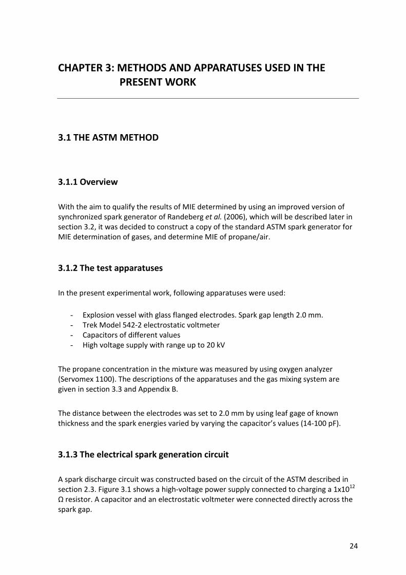
A spark discharge circuit was constructed based on the circuit of the ASTM described in
section 2.3. Figure 3.1 shows a high-voltage power supply connected to charging a 1x10¹²
Ω resistor. A capacitor and an electrostatic voltmeter were connected directly across the
spark gap.
Page 31
25
Figure 3.1: Block diagram of the electric spark circuit of ASTM for determination of MIE for gases
and vapours. From Litchfield (1967)
3.1.4 Determination of spark energy
After the gas mixture of the desired concentration has been loaded into the explosion
vessel, the applied voltage across the spark gap was increased gradually until a sparks
occurred.
Some introduction experiments were performed with the aim to find the spark
breakdown voltage in air for 2.0 mm spark gap length. According to Babrauskas (2003),
for a spark gap distance of 2.0 mm the breakdown voltage is around 6.0 kV. Due to the
statistical nature of spark discharges, the breakdown occurs at different voltages even for
apparently identical test conditions. In the present work, the breakdown voltages for the
2.0 mm spark gap were in the range of 6.0-7.0 kV.
The spark energy E was calculated by:
E = ½ CU2 (3.1)
Where C is the energy storage capacitance, the sum of the capacitance of the electrode
gap and the stray capacitance. U is the spark voltage at the moment of discharge,
measured by a Strek- electrostatic voltmeter. C and U have the standard units of F (Farad)
and V (Volt). This yields E in J (Joule). In the present work, the stray capacitance is
estimated to be about 2.0 pF.
Page 32
26
3.2 THE NEW SYNCHRONIZED SPARK GENERATOR METHOD
3.2.1 Overview
Randeberg et al. (2006) described a spark generator, which was claimed to be able to
produce synchronized capacitive spark discharges of low energies down to 0.03mJ.
However, Eckhoff et al. (2008) re-examined the discharge circuit of Randeberg et al. and
concluded that the real spark energies in the experiments by Randeberg and Eckhoff
(2007) were much larger than those quoted in their paper. In fact, the additional energy
was of order of 1 mJ. Figure 3.2 shows the pulse generated by the synchronized spark
generator of Randeberg et al., as described by Eckhoff et al..
In the present investigation, an improved version of the synchronized spark generator of
Randeberg et al. has been constructed. The aim of the improvement has been to
minimize the additional energy contribution to the effective spark energy. Figure 3.3
shows the pulse produced by the new synchronized spark generator. At spark discharge,
the pulse over the spark gap is as shown in Figure 3.4.
Figure 3.2: Pulse produced by
the synchronized spark
generator of Randeberg et al.
(2006). The main pulse has
duration of about 100 ns and
peek voltage of about 6 kV.
The tail of the pulse has
voltage of about 650 V and
duration of 50-100 μs.
Figure 3.3: Pulse produced by the
new spark generator. The 2-3 μs
main pulse has a voltage of about
10 kV. The residual pulse has a
voltage of about 650 V and
duration from 1 to 3 μs.
Figure 3.4: Pulse produced
by the new spark generator.
At spark discharge, the
undershoot of the pulse
from Figure 3.3 is
eliminated.
Page 33
27
3.2.2 Test apparatuses
The experimental set-up consisted of the following apparatuses:
- Explosion vessel with glass flanged electrodes. Spark gap length 2.0 mm.
- Capacitors of different values
- Voltage supplies
- High voltage probe Tektronix P6015, P6015A and P6013A
- Philips pulse generators, PM 5705 and PM 5715.
- Tektronix TDS 3034B oscilloscope
Propane concentration in the tested mixture was measured by a Servomex 1400 gas
analyser, based on infrared light absorption. For the descriptions of the apparatuses and
the gas mixing system used in this experimental work refer to section 3.3 and Appendix B.
3.2.3 Electrical spark-generation circuit
Figure 3.5 illustrates the experimental setup of a new synchronized spark-generation
circuit. The circuit has been developed by senior engineer Werner Olsen at UoB,
Department of Physics and Technology. The detailed circuit diagrams of the different sub-
circuit in Figure 3.5 are given in Appendix C.
When the system is triggered, the pulse generator P1 generates two tailored pulses of 60
μs duration 240 μs apart. The first pulse then triggers pulse generator P2, whereas the
second pulse triggers pulse generator P3.
The pulse from pulse generator P2 is a 0.24 V rectangular pulse of 260 μs duration, which
passes through amplifier A1 before entering the primary windings of the high voltage
transformer T1. Figure 3.6a illustrates a typical output signal from T1. The simple diode
circuit F1 filters out the first negative part of the pulse. The second positive part of the
pulse has a peak voltage of about 400 V and for the simplicity of later description this
pulse is called pulse I.
Page 34
28
Figure 3.5: Schematic block diagram of the improved version of the synchronized spark generator
of Randeberg et al. (2006). A1-A5 are the amplifiers. T1 and T2 are high-voltage transformers. P1
is a tailor-made pulse generator. P2 and P4 are Philips pulse generators PM5715. P3 are Philips
pulse generator PM 5705.
The output from pulse generator P3 is a short-duration (0.06 μs) pulse with amplitude
about 13V, which triggers pulse-generator P4 that produces a low voltage pulse (2.5V) of
8.0 μs duration and rectangular shape as illustrated in Figure 3.6b.
The pulses produced by P3 and P4 are both sent to amplifier A2, where they are amplified
about 7.5 times and combined to one signal. Figure 3.6c shows the dual-peak signal from
amplifier A2. The first peak originates from the pulse generated by P3 and is now about
90V. The second peak originates from the signal from P4 and is now about 19 V.
The dual-peak signal illustrated in Figure 3.6c enters amplifier A3 where it is inverted by a
NPN transistor and the amplitude amplified from 90 to about 500 V. Figure 3.6d shows
the two-peak pulse from Figure 3.6c has now become a single peak pulse with a “knee”.
The pulse from amplifier A3 is sent to the high-voltage transformer T2. A diode is
introduced in the circuit to minimize the amplitude of the undershoot. With the aim to
Page 35
29
shorten the duration of the high-voltage pulse, the iron core of the high-voltage
transformer in this circuit is replaced by ferrite core. Figure 3.6e shows the pulse is
transformed to a single-peak high-voltage pulse of about 10 kV and duration about 4-6 μs.
The amplitude of the undershoot is about 500 V. This pulse signal is then combined with
pulse I (+ 400V) to produce a final undershoot of about 100V.
Due to the high-voltage sensitivity of diode, the pulse signal of 10 kV and undershoot of
100V are then reduced by a factor of 1000 by the mean of a Tektronix P6015 high-voltage
probe. It appears that it would be more appropriate reduce the voltage by a factor of 100
or 200, but in the present work, a factor of 1000 was used due to the availability of the
high-voltage probe.
Filter F2 eliminates the 10 kV peak of the pulse-signal after it has been reduced to a 10V
peek pulse. The remaining undershoot is sent to amplifiers A4 and A5. The aim is to
amplify it 1000 times to recover its original shape and amplitude, so that the undershoot
from both sides of the spark gap can eliminate each other.
The function of the RC-circuit H is to offset the DC level.
By placing two high-voltage measurement probes as shown in Figure 3.5, the shapes and
magnitudes of the pulses from both sides of the spark gap and spark occurrence are
recorded by the mean of a Tektronix TDS 3034B oscilloscope.
Figure 3.6f shows the pulse signal at spark discharge. The main pulse would be about 10
kV, with duration 2-3 μs.
Prior to spark discharge, the voltage gradually increases until the spark occurs and then
drops rapidly to 0. However, the residual part of the input pulse causes the voltage to
increase and stabilize at about 600- 650 V. This resulting additional energy supply is
denoted as the residual pulse and has a duration about 1-3 μs, depending on when the
spark gap breakdown occurs.
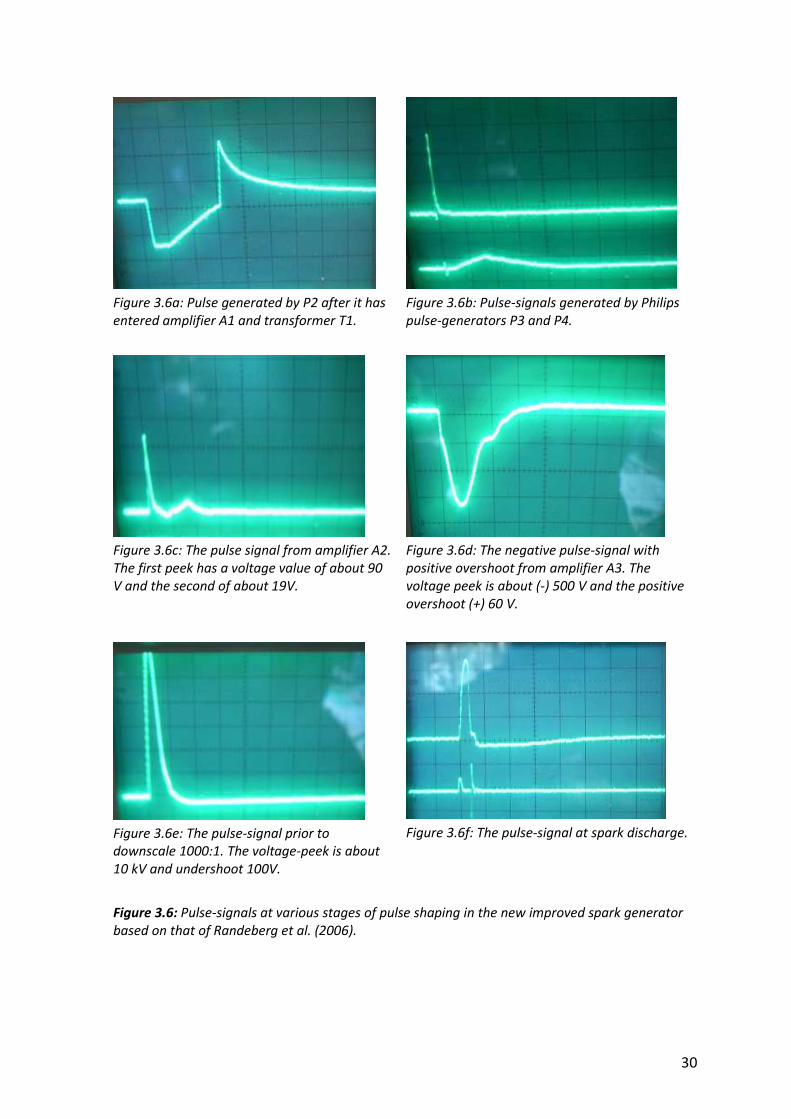
Page 36
30
Figure 3.6a: Pulse generated by P2 after it has
entered amplifier A1 and transformer T1.
Figure 3.6b: Pulse-signals generated by Philips
pulse-generators P3 and P4.
Figure 3.6c: The pulse signal from amplifier A2.
The first peek has a voltage value of about 90
V and the second of about 19V.
Figure 3.6d: The negative pulse-signal with
positive overshoot from amplifier A3. The
voltage peek is about (-) 500 V and the positive
overshoot (+) 60 V.
Figure 3.6e: The pulse-signal prior to
downscale 1000:1. The voltage-peek is about
10 kV and undershoot 100V.
Figure 3.6f: The pulse-signal at spark discharge.
Figure 3.6: Pulse-signals at various stages of pulse shaping in the new improved spark generator
based on that of Randeberg et al. (2006).
Page 37
31
3.2.4 Determination of spark energy
The same flanged electrode system as used in the ASTM test was used. The spark gap was
set to 2.0 mm. After the explosion vessel had been filled with gas mixture of the desired
concentration, the spark generator was triggered. If the spark triggering is not successful
at first trail, triggering is repeated with 15-20 s intervals until the spark occurs. The 15-20
s interval is necessary to ensure that the energy supplied by the preceding pulse has
dissipated. The spark energy is varied by varying the value of the connected capacitor.
The spark energy E was calculated by:
E = E1 + E2 = ½ CU12 + ∫ U2i dt (3.2)
Hence the first term E1 is the energy contained in the main pulse, C being the storage
capacitance and U1 the voltage at spark gap at the moment of breakdown. The stray
capacitance is estimated to be about 2 pF and must be included in the storage
capacitance for the calculation of E1. The second term E2 is the additional energy
contribution from the residual pulse. U2 is the voltage and i the current. The duration of
the residual pulse i.e. the duration of the additional energy to the spark channel varies
from 1 to 3 μs, depending on the time when the spark occurs.
When the input voltage U0 to a RC-circuit is known, the output voltage U1 can be
calculated in accordance with the analogue-block-diagram illustrated in Figure 3.7. The
discharge voltage U1 is then estimated by following equation:
U1 = RC
1 ∫ (U0 – U1) dt
(3.3)
R being the resistance and C the capacitance connected to the spark gap. U0 is the pulse
voltage measured by placing the high-voltage probe upstream of the spark gap as shown
in Figure 3.5.
Figure 3.7: Analogue-block-diagram of the RC-circuit
Page 38
32
The current i in the residual pulse is estimated by:
i = R2
650U
R2
UU 121 −=
−
(3.4)
Equation 3.4 shows that i is the average current, strongly influenced by the discharge
voltage U1 and the resistance R connected to the spark gap. Based on the work of Kleppa
(2008) and the present work, U2 has value of about 600-650 V. In the present calculations,
the value 650 V was used. For a typical discharge voltage U1 of 10 kV, the current i in the
residual pulse has a value of about 0.12 A when a 39 kΩ resistor is inserted prior to the
spark gap. By increasing the resistance to 110 kΩ, i decreases to 0.04 A.
3.3 APPARATUSES
3.3.1 The explosion vessel
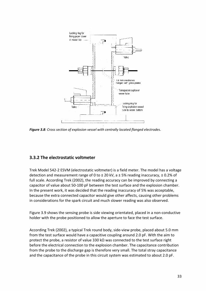
Figure 3.8 shows the cross section of the explosion vessel used in the present work. The
reaction vessel is a cylindrical hard plastic tube with inner diameter of 40 mm and height
of 156 mm, corresponding to a net internal volume of 0.20 dm3. The inlet tube with the
valve is placed in the bottom and the outlet tube on the top of the explosion vessel.
Two 1.6 mm flat ended tungsten electrodes flanged with glass plates are located at the
centre of the tube. One is fixed while the other is moveable, allowing adjustment of the
gap distance between the electrodes. The electrode tips screw into stainless steel rods,
which extends through the wall of the explosion vessel, allowing external electrical
connections.
The glass flanges were made of borosilicate glass and have a diameter of 15 mm and
thickness of about 3.0 mm. They were fastened to the electrodes with Araldite. A locking
ring for fixing a paper cover is placed at the top of the vessel.
Page 39
33
Figure 3.8: Cross section of explosion vessel with centrally located flanged electrodes.
3.3.2 The electrostatic voltmeter
Trek Model 542-2 ESVM (electrostatic voltmeter) is a field meter. The model has a voltage
detection and measurement range of 0 to ± 20 kV, a ± 5% reading inaccuracy, ± 0.2% of
full scale. According Trek (2002), the reading accuracy can be improved by connecting a
capacitor of value about 50-100 pF between the test surface and the explosion chamber.
In the present work, it was decided that the reading inaccuracy of 5% was acceptable,
because the extra connected capacitor would give other affects, causing other problems
in considerations for the spark circuit and much slower reading was also observed.
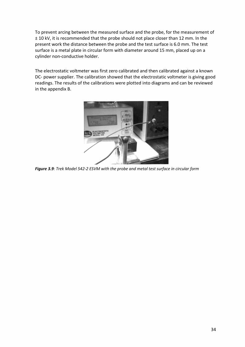
Figure 3.9 shows the sensing probe is side viewing orientated, placed in a non-conductive
holder with the probe positioned to allow the aperture to face the test surface.
According Trek (2002), a typical Trek round body, side-view probe, placed about 5.0 mm
from the test surface would have a capacitive coupling around 2.0 pF. With the aim to
protect the probe, a resistor of value 330 kΩ was connected to the test surface right
before the electrical connection to the explosion chamber. The capacitance contribution
from the probe to the discharge gap is therefore very small. The total stray capacitance
and the capacitance of the probe in this circuit system was estimated to about 2.0 pF.
Page 40
34
To prevent arcing between the measured surface and the probe, for the measurement of
± 10 kV, it is recommended that the probe should not place closer than 12 mm. In the
present work the distance between the probe and the test surface is 6.0 mm. The test
surface is a metal plate in circular form with diameter around 15 mm, placed up on a
cylinder non-conductive holder.
The electrostatic voltmeter was first zero calibrated and then calibrated against a known
DC- power supplier. The calibration showed that the electrostatic voltmeter is giving good
readings. The results of the calibrations were plotted into diagrams and can be reviewed
in the appendix B.
Figure 3.9: Trek Model 542-2 ESVM with the probe and metal test surface in circular form
Page 41
35
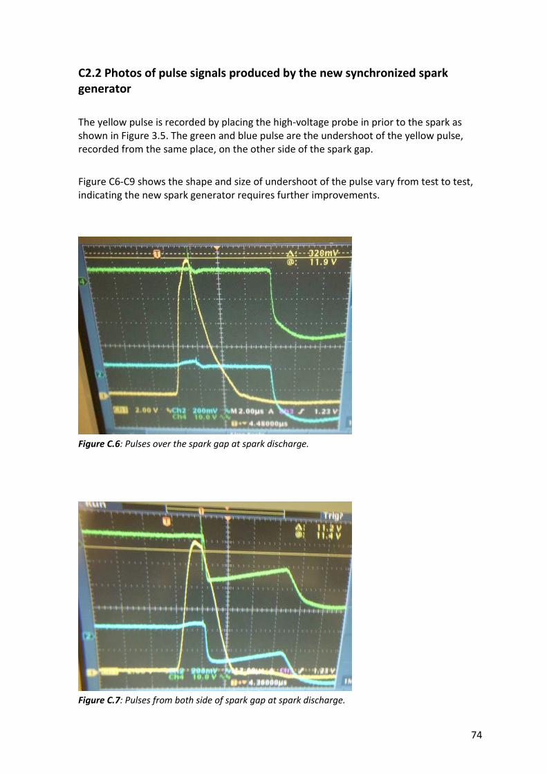
CHAPTER 4: RESULTS AND DISCUSSION
4.1 RESULTS OBTAINED WITH THE ASTM CIRCUIT
4.1.1 Determination of MIE as a function of propane/air concentration
About 220 tests were done to determine the minimum ignition energy for propane/air.
The propane concentration range covered was in the 3.5-8.0 vol. %. The main aim of the
tests was to find the boundary between ignition and no-ignition across the investigated
concentration range.
The spark energy values were calculated from equation 3.1 (E = ½ CU2).
By using the same method for identifying the minimum ignition energy of Moorhouse et
al. (1974), the highest possible border line was drawn through the array of experimental
data points, below which there was no ignition point. In this way, the U-shaped curve
shown in Figure 4.1 was obtained. The data points inside (above) the U-shaped curve
contain both ignition and no-ignition data. The minimum of this U-shaped curve indicates
a minimum ignition energy of about 0.50 mJ for propane concentrations in the range of
5.0-5.5 vol. %.
Figure 4.1 also shows that the spark gap distance of 2.0 mm used in the present work was
the quenching distance for a propane concentration of about 4.2 vol. %. No ignition was
observed for propane concentration lower than 4.2 vol. %, even if the spark energy was
increased significantly. On the other hand, the present results do not indicate that 2.0
mm is the quenching distance for any specific concentration on the fuel rich side. The
experimental results showed that ignition was still obtained by increasing the spark
energy for mixtures up to around 8.0 % vol.
According to the study of Lewis and von Elbe (1961), see Figure 2.1 in section 2.1, the
quenching distance should also be a U-shaped function of propane concentration. For a
given pressure, every concentration of the mixture corresponds to a certain quenching
distance. At ambient conditions (1 amt pressure), a spark gap of 2.0 mm seems to have a
quenching effect for propane/air mixtures of around 4.0 and 6.0 vol. %.
The result obtained with the ASTM method in the present work was also compared with
results reported by Moorhouse et al. (1974) and Lewis and von Elbe (1961). Figure 4.2
Page 42
36
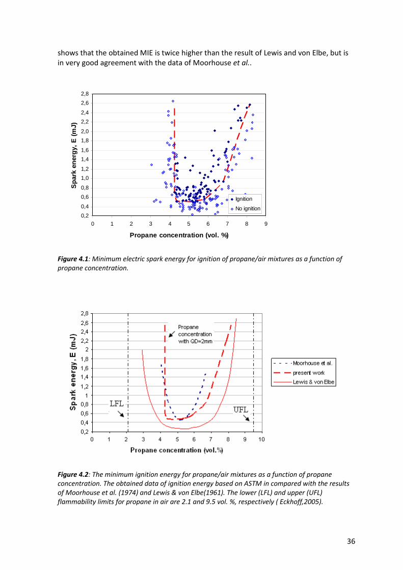
shows that the obtained MIE is twice higher than the result of Lewis and von Elbe, but is
in very good agreement with the data of Moorhouse et al..
0,2
0,4
0,6
0,8
1,0
1,2
1,4
1,6
1,8
2,0
2,2
2,4
2,6
2,8
0 1 2 3 4 5 6 7 8 9
Propane concentration (vol. %)
Sp
ark
ener
gy,
E (
mJ)
Ignition
No ignition
Figure 4.1: Minimum electric spark energy for ignition of propane/air mixtures as a function of
propane concentration.
Figure 4.2: The minimum ignition energy for propane/air mixtures as a function of propane
concentration. The obtained data of ignition energy based on ASTM in compared with the results
of Moorhouse et al. (1974) and Lewis & von Elbe(1961). The lower (LFL) and upper (UFL)
flammability limits for propane in air are 2.1 and 9.5 vol. %, respectively ( Eckhoff,2005).
Page 43
37
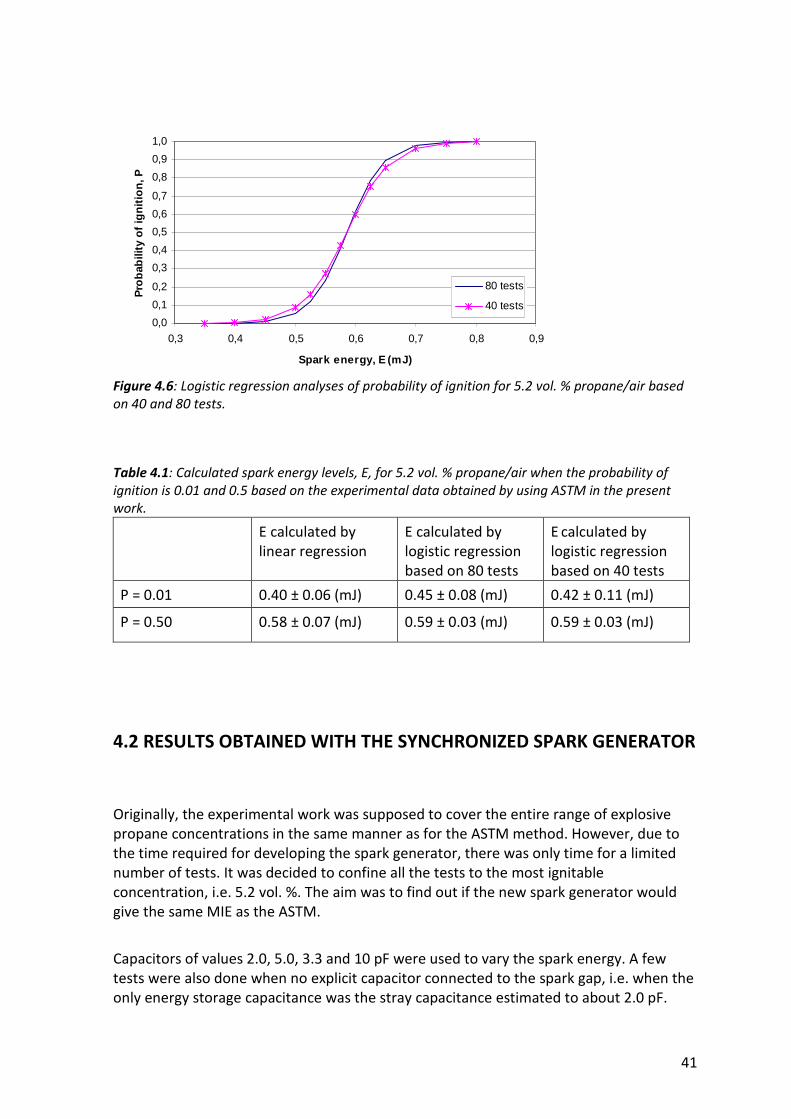
4.2.2 Determination of probability of ignition
The discrepancy between the MIE value of 0.25 mJ claimed by Lewis and von Elbe (1961)
and the value 0.46 mJ found by Moorhouse et al. (1974) called for a closer investigation
of whether this could be due to different statistical treatment of the data. According to
Moorhouse et al., Lewis and von Elbe’s MIE values referred to 1 % probability of ignition.
It was therefore decided to perform a statistical analysis of the experimental data
obtained for 5.5 and 5.2 vol. % propane in air.
The first test series was performed with 5.5 % vol. propane/air mixture, and 20 tests were
done for each different spark energy levels by varying capacitors of values 14.0, 19.0, 23.0
and 28.6 pF. No ignition was observed with the 14.0 pF capacitor, or a spark energy of
0.33 ± 0.04 mJ. By increasing the value of the connected capacitor to 19.0 pF, the applied
spark energy was increased to 0.41 ± 0.05 mJ, but still no ignition was observed. The same
numbers of tests were performed with capacitors of value 23.0 pF (0.53 ± 0.06 mJ) and
28.6 pF (0.76 ± 0.06 mJ), obtaining ignition probabilities of 25 % and 100 %, respectively.
The second test series were done with 5.2 % vol. propane/air mixture. The results showed
no significant difference in the probability of ignition for mixture concentration of 5.5 and
5.2 vol. %, even though it was expected that the mixture of 5.2 vol. % would be slightly
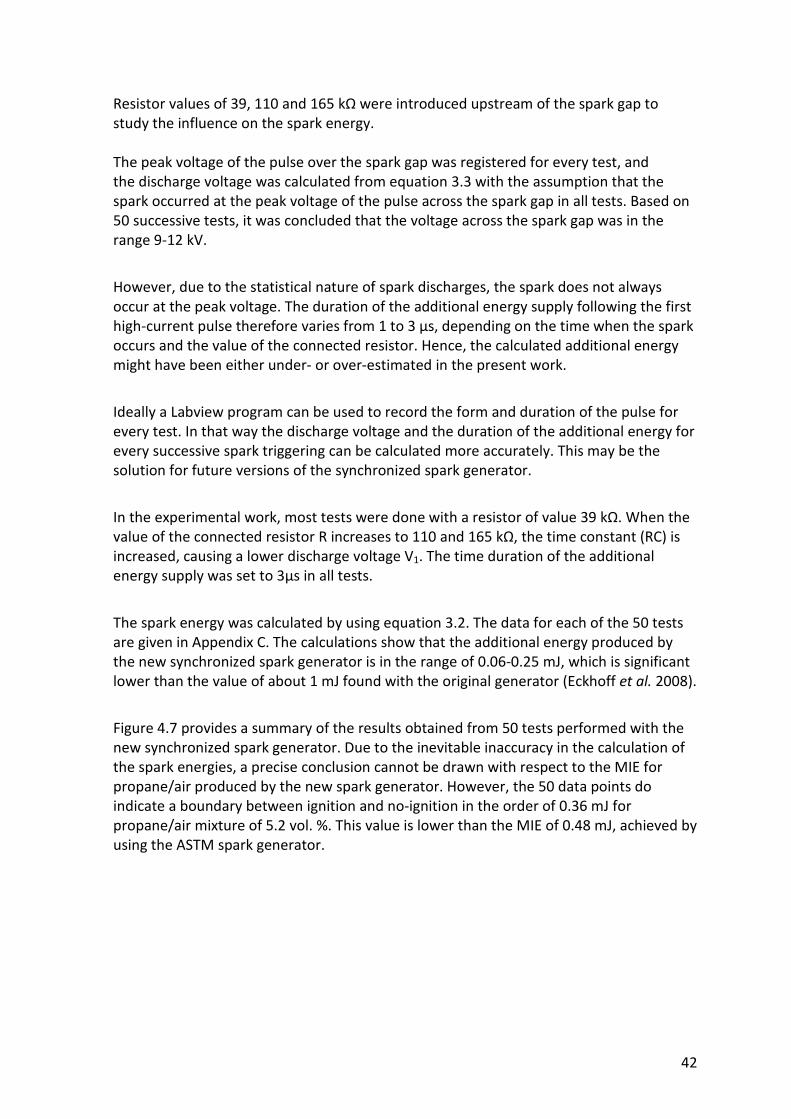
more ignitable. Both mixture concentrations had an ignition probability of 25% when
using the capacitor of value 23.0 pF. The spark energy level for 5.5 vol. % mixture was
0.53 ± 0.06 mJ and for 5.2 vol. % 0.49 ± 0.09 mJ. It is also important to emphasis that the
probability of ignition is strongly dependent on the stability of the spark i.e. the voltage
deposit in the spark.
In figures 4.3 and 4.4 the probabilities of ignition (y-axis) are plotted as function of the
arithmetic mean spark energy values for each series of 20 tests and their standard
deviations (x-axis). The ignition probabilities are calculated from equation 2.7 (P=m/n). A
linear regression trend line is added with respect to the average values of ignition energy.
The results suggest that the probability of ignition is a linear function of the spark energy,
where the ignition probability of a mixture increases when higher spark energy is applied.
Page 44
38
0.76 mJ, 28.6 pF
0.53 mJ, 23.0 pF
0.41mJ, 19.0 pF
y = 2.8675x - 1.209
0 %
10 %
20 %
30 %
40 %
50 %
60 %
70 %
80 %
90 %
100 %
0 0,1 0,2 0,3 0,4 0,5 0,6 0,7 0,8 0,9
Spark energy, E (mJ)
Pro
bab
ilit
y o
f ig
nit
ion
, P
Figure 4.3: Probability of ignition for 5.5 vol. % propane/air. The average value of ignition energy
and the values of the capacitors connected to the spark gap are noted in the diagram.
0.49 mJ, 23.0 pF
0.40 mJ,19.0 pF
0.76 mJ, 28.6 pF
0.66 mJ, 28.6pF
y = 2.758x - 1.1009
0 %
10 %
20 %
30 %
40 %
50 %
60 %
70 %
80 %
90 %
100 %
0,00 0,10 0,20 0,30 0,40 0,50 0,60 0,70 0,80 0,90
Spark energy, E(mJ)
Pro
bab
ilit
y o
f ig
nit
ion
, P
Figure 4.4: Probability of ignition for 5.2 vol. % propane/air. The average value of ignition energy
and the values of the capacitors connected to the spark gap are also noted in the diagram.
Page 45
39
Ignition probability calculated by using logistic/binary regression
According to statistic literature, logistic regression is a convenient approach for modelling
binary response and it is used extensively in the biological sciences, biomedical research,
as well as in engineering.
The probability of ignition for 5.2 vol. % propane/air mixtures was calculated by using
equation 2.8. The upper and lower limits for the 95% confidence envelope (UCL and LCL)
were calculated by using equation 2.10, and the results are plotted in Figure 4.5 as a
function of the spark energy.
The values of β0, β1, ρ and standard deviations of β0 and β1 in equation 2.8 and 2.10 can
be found by using statistical tools SAS, PROC or SPSS. In the present work, SPSS (Statistical
Package for the Social Sciences) was used. The variances σ00 and σ01 were calculated as
the square of the standard deviations. Based on the data from 80 tests for 5.2 vol. %
propane mixture, SPSS gave β1 = 33.070 and β0 = -19.370, ρ = -0.995 and standard
deviations for β0 and β1 of 5.142 and 8.677, respectively.
P(E) = i10 Ee1
1β−β−+
=iE070.33370.19e1
1−+
(2.8)
LCLUCL = E ± zα/2 2
1112
0100 /)EE2( βσ+σ+σ (2.10)
Where
σ01 = ρ 1100σσ = -0.995 22 677.8142.5 = - 44.394
and
LCLUCL = E ± 1.96 2222 )070.33/()677.8E)394.44(E2142.5( +−+
Figure 4.5 shows the logistical probability distribution and the 95% confidence envelope
for spark energy of 5.20 vol. % propane/air mixture. Probability of ignition, P (y-axis) is
plotted as a function of spark energy, E (x-axis). The figure reveals the S-shaped function
that approaches P = 1.0 as an asymptote. The original experimental data are also plotted
in the diagram. For a given spark energy, E, the ignition probability, P(E) is unity for
ignition and zero for no-ignition. Based on the data obtained in the present work, the
most interesting ignition energy levels are in the range of 0.50-0.65 mJ, where ignition
and no-ignition data overlap.
Page 46
40
0,0
0,1
0,2
0,3
0,4
0,5
0,6
0,7
0,8
0,9
1,0
0,3 0,4 0,5 0,6 0,7 0,8 0,9
Spark energy, E (mJ)
Pro
babi
lity
of ig
nitio
n, P
Figure 4.5: Logistical probability distribution and 95% confidence envelope for spark ignition data
of 5.2 % vol. propane/air mixture. The original data are also plotted in the diagram. For given
spark energies E, probability of ignition is 1 for “ ignition” and 0 for “ no-ignition”.
Logistic regression was also used to calculate the probability for the ignition of 5.2 vol. %
mixture based on the 40 test data, where most energy levels for ignition and non-ignition
overlap. The analysis gave β1 = 27.743, β0 = - 16.240, ρ = -0.996, and standard deviations
for β0 and β1 of 5.334 and 9.046, respectively. The probability of ignition and the upper
and lower critical limits were also calculated by using equation 2.8 and 2.10. Figure 4.6
shows that the S-shaped curve based on 80 tests is a little bit steeper than the one based
on 40 tests, otherwise the two S-curves are quite similar. When the probability of ignition
is in the range 40-60%, the two S-curves give practically the same calculated spark energy
level.
Lewis and von Elbe used a probability of ignition of 1% and obtained a MIE value of order
0.25 mJ for 5.2 vol. % propane/air. By using linear and logistic regression methods, the
corresponding energy levels based on the present data were calculated. The results are
listed in Table 4.1. The calculated values of spark energy for probabilities of ignition of 1%
and 50% indicated that the two probability calculation methods give almost the same
results. According to the calculated data obtained by using logistic regression, for 1%
probability of ignition, the spark energy is in the relatively wide range of 0.42 ± 0.11 mJ.
In the present study, it has not been possible to trace any statistical information in the
work of Lewis and von Elbe. Therefore it is not clear which method Lewis and von Elbe did
use to obtain the exact MIE value for propane/air of 0.25 mJ for a 1% probability of
ignition. In particular, it is not known whether the value was obtained experimentally or
via some mathematical model of ignition frequency as a function of spark energy.
Page 47
41
0,0
0,1
0,2
0,3
0,4
0,5
0,6
0,7
0,8
0,9
1,0
0,3 0,4 0,5 0,6 0,7 0,8 0,9
Spark energy, E (mJ)
Pro
bab
ility
of
ign
itio
n, P
80 tests
40 tests
Figure 4.6: Logistic regression analyses of probability of ignition for 5.2 vol. % propane/air based
on 40 and 80 tests.
Table 4.1: Calculated spark energy levels, E, for 5.2 vol. % propane/air when the probability of
ignition is 0.01 and 0.5 based on the experimental data obtained by using ASTM in the present
work.
E calculated by
linear regression
E calculated by
logistic regression
based on 80 tests
E calculated by
logistic regression
based on 40 tests
P = 0.01 0.40 ± 0.06 (mJ) 0.45 ± 0.08 (mJ) 0.42 ± 0.11 (mJ)
P = 0.50 0.58 ± 0.07 (mJ) 0.59 ± 0.03 (mJ) 0.59 ± 0.03 (mJ)
4.2 RESULTS OBTAINED WITH THE SYNCHRONIZED SPARK GENERATOR
Originally, the experimental work was supposed to cover the entire range of explosive
propane concentrations in the same manner as for the ASTM method. However, due to
the time required for developing the spark generator, there was only time for a limited
number of tests. It was decided to confine all the tests to the most ignitable
concentration, i.e. 5.2 vol. %. The aim was to find out if the new spark generator would
give the same MIE as the ASTM.
Capacitors of values 2.0, 5.0, 3.3 and 10 pF were used to vary the spark energy. A few
tests were also done when no explicit capacitor connected to the spark gap, i.e. when the
only energy storage capacitance was the stray capacitance estimated to about 2.0 pF.
Page 48
42
Resistor values of 39, 110 and 165 kΩ were introduced upstream of the spark gap to
study the influence on the spark energy.
The peak voltage of the pulse over the spark gap was registered for every test, and
the discharge voltage was calculated from equation 3.3 with the assumption that the
spark occurred at the peak voltage of the pulse across the spark gap in all tests. Based on
50 successive tests, it was concluded that the voltage across the spark gap was in the
range 9-12 kV.
However, due to the statistical nature of spark discharges, the spark does not always
occur at the peak voltage. The duration of the additional energy supply following the first
high-current pulse therefore varies from 1 to 3 μs, depending on the time when the spark
occurs and the value of the connected resistor. Hence, the calculated additional energy
might have been either under- or over-estimated in the present work.
Ideally a Labview program can be used to record the form and duration of the pulse for
every test. In that way the discharge voltage and the duration of the additional energy for
every successive spark triggering can be calculated more accurately. This may be the
solution for future versions of the synchronized spark generator.
In the experimental work, most tests were done with a resistor of value 39 kΩ. When the
value of the connected resistor R increases to 110 and 165 kΩ, the time constant (RC) is
increased, causing a lower discharge voltage V1. The time duration of the additional
energy supply was set to 3μs in all tests.
The spark energy was calculated by using equation 3.2. The data for each of the 50 tests
are given in Appendix C. The calculations show that the additional energy produced by
the new synchronized spark generator is in the range of 0.06-0.25 mJ, which is significant
lower than the value of about 1 mJ found with the original generator (Eckhoff et al. 2008).
Figure 4.7 provides a summary of the results obtained from 50 tests performed with the
new synchronized spark generator. Due to the inevitable inaccuracy in the calculation of
the spark energies, a precise conclusion cannot be drawn with respect to the MIE for
propane/air produced by the new spark generator. However, the 50 data points do
indicate a boundary between ignition and no-ignition in the order of 0.36 mJ for
propane/air mixture of 5.2 vol. %. This value is lower than the MIE of 0.48 mJ, achieved by
using the ASTM spark generator.
Page 49
43
0,00
0,10
0,20
0,30
0,40
0,50
0,60
0,70
0,80
0,90
1,00
0 10 20 30 40 50
Test number
Sp
ark
ener
gy
(mJ)
No-ignition
Ignition
Figure 4.7: Experimental spark energy data of 5.2 vol. % propane/air mixtures achieved by using
the improved synchronized spark generator of Randeberg et al. (2006).
Page 50
44
CHAPTER 5: CONCLUSIONS AND SUGGESTIONS FOR FURTHER
WORK
5.1 CONCLUSIONS FROM APPLYING THE ASTM METHOD FOR MIE
DETERMINATION
1. A study of the literature revealed a discrepancy between the classical MIE value for
propane/air of 0.25 mJ reported by Lewis and von Elbe (1961), and the value of 0.46 mJ
found by Moorhouse et al. (1974). According to the latter workers, Lewis and von Elbe
defined their MIEs as the spark energy yielding an ignition probability of only 1 %.
Moorhouse et al. adopted a pragmatic criterion for determining MIE, based on drawing
the highest possible border line through their array of experimental ignition/no ignition
points, below which there were no ignitions. The minimum value of this U-shaped border
line was taken as the MIE.
2. In the present experimental investigation, using the pragmatic criterion suggested by
Moorhouse et al. and a copy of ASTM’s spark circuit, the MIE for propane in air was found
to be 0.48 mJ. This is in very close agreement with the value found by Moorhouse et al.,
but twice the value reported by Lewis and von Elbe.
3. The experimental data also showed that the gap of 2.0 mm between the flanged
electrodes equals the quenching distance for a propane/air mixture of around 4.0 vol. %
on the fuel lean side, which is in good agreement with the results of Lewis and von Elbe.
On the other hand, it was not possible to define any specific propane concentration on
the fuel rich side for which the quenching distance was 2.0 mm. Lewis and von Elbe
claimed that on the fuel rich side 2.0 mm would be the quenching distance for 6.0 vol. %
propane in air.
4. In the present investigation, the most easily ignitable propane concentration was about
5.2 vol. %, but 5.5 vol. % gave practically identical result.
5. The probability of ignition increases with spark energy. By applying a logistic regression
analysis to the data obtained for 5.2 vol. % and 5.5 vol. % respectively, the spark energies
giving 1% and 50 % probability of ignition were calculated. The spark energy giving 50 %
probability of ignition was 0.59 ± 0.03 (mJ), whereas that giving 1 % probability was 0.42 ±
0.11 (mJ). The calculated MIE value for 1 % probability of ignition of 0.42 mJ is
significantly higher than the value of 0.25 mJ of Lewis and von Elbe.
Page 51
45
5.2 CONCLUSION FROM APPLYING THE SYNCHRONIZED SPARK
GENERATOR FOR MIE DETERMINATION
A modified version of the synchronized spark generator described by Randeberg et al.
(2006) was constructed. However, due to considerable challenges during this work, there
was only time left for a limited series of ignition experiments with propane/air, using a
preliminary prototype of the generator. The data obtained indicate a border line between
ignition and no-ignition of about 0.36 mJ for mixture of 5.2 vol. % propane in air. So far,
the residual energy produced by the new synchronized spark generator is significantly
lower than for the original one, typically 0.25 mJ as opposed to the original 1 mJ.
5.3 SUGGESTIONS FOR FURTHER WORK FOR THE SYNCHRONIZED
SPARK GENERATOR
During the experimental test program, there were many non-successful attempts at
triggering the spark. The high-voltage transformer T2 should therefore have more
secondary windings to achieve voltages higher than 12 kV, and hence more reliable spark
triggering. It should also be considered to use needle shaped electrodes tips to lower the
breakdown voltage.
All the pulse generators (P1-P4 in Figure 3.2) can in principle be replaced by a crystal
oscillator to achieve a more precise time reference. In the present work, one pulse is used
to trigger another, and the time reference of the pulse generators are based on an
analogue RC-system. Limited precision with respect to timing may affect the shape and
amplitude of the pulse across the spark gap and cause inaccuracy in the energy
calculation.
A high-voltage probe with a scale-down ratio of 100:1 or 200:1 should replace the high-
voltage probed with a scale-down of 1000:1 used in the present work. This would simplify
the process of amplifying the tail of the pulse to recover its original shape and amplitude,
and eliminate some of the inaccuracies in the present system.
Calculations suggest that the residual energy may decrease from about 0.25 mJ to less
than 0.1 mJ by increasing the value of the resistor connected in series with the spark gap
from 39 kΩ to 110-165 kΩ. This should be explored further in the future studies.
A Labview program can be connected to the oscilloscope that registers the spark
occurrence for every test. The duration of the residual pulse i.e. the duration of the
additional energy can thereby be estimated and the calculated spark energy will be more
accurate.
Page 52
46
It is recommended that a complete series of ignition tests for propane/air be undertaken
with the new version of the modified synchronized spark generator.
Page 53
47
LIST OF REFERENCES
ASTM (2007): Standard test method for minimum ignition energy and quenching distance
in gaseous mixtures. Designation E 582-07. ASTM Int.
Babrauskas, V. (2003): Ignition Handbook, Published by Fire Science Publishers, A division
of Fire Science and Technology Inc., Issaquad, WA 98027, USA.
Blanc V. M., Guest P. G., von Elbe G and Lewis B. (1947): J. Chem. Phys. 15, 798; “Third
Symposium on Combustion and Flame and Explosion Phenomena”, pp. 363, William &
Wilkins, Baltimore, 1949.
Calcote H. F., Gregory C.A., Barnett, and Gilmer (1952): Spark ignition, Effect of Molecular
Structure. Industrial and engineering chemistry 44 (1952).
Cheng, D. Y (1967): the name of the article was not possible to trace in this present work,
Combustion Flame, Vol. 11, pp. 517.
Crowl, D. (2003): Understanding explosions, American Institute of Chemical Engineers.
Eckhoff, R. K. (1970): The energy required for the initiation of explosions in dust clouds by
electric sparks, M.Phil. Thesis, University of London.
Eckhoff, R. K. (2003): Dust Explosion in Process industries, 3rd
edition, Gulf Professional
Publishing. ISBN 0-7506-7602-7
Eckhoff, R. K. (2005): Explosion Hazards in process industries, 1st
edition, Houston, Texas,
Gulf Publishing Company. ISBN 0-9765113-4-7
Eckhoff R. K., Olsen W. and Kleppa O. (2008): Influence of spark discharge duration on the
minimum ignition energy of premixed propane/air, Proc. 7th
International Symposium on
Hazards, Prevention and Mitigation of Industrial Explosions. St Petersburg, Russia, July
2008. Published by Semenov Institute of Chemical Physics.
Glor, M. (1984): Condition for the appearance of discharges during the gravitational
compaction of powders, J. Electrostatic 15, pp. 223 – 235.
Guest, P. G. (1944): U.S. Bur. Mines, Rept. Invest. 3753.
Kleppa O. (2008): Minimum ignition energy of propane/air, Master thesis (in Norwegian)
submitted to University of Bergen, Norway.
Page 54
48
Kono M., Kumagai and Sakai T. (1976): The optimum condition for ignition of gases by
composite sparks, Proc. 16th
Symposium (international) on combustion, pp. 757-766, The
Combustion Institute, Pittsburgh, USA.
Kono, M. and Hatori, K. (1985): Ignition of low flow velocity mixture by short duration
sparks, pp. 500 – 503 in GD85 – 8th
Intl. Conf. on Gas Discharges & Their Applications,
Leeds Univ. Press, Leeds.
Kono M., Isshii K., Tsukamoto T. and Ujiie Y. (1992): Analysis of ignition mechanism of
combustible mixtures by composite sparks, Combustion and Flame, Vol. 91, pp. 153-164
(1992).
Ko, Y., Anderson R.W. and Arpaci V.S (1991): Spark ignition of propane/air mixtures near
the minimum ignition energy: Part I. An experimental study, Combustion and flame, Vol.
83, pp. 75-87.
Kravchenko, V.S, Serov (1980): Chapter 3. Ignition of explosive mixtures by electric
discharges, The relationship between the ignition energy and the duration of its release,
Health and Safety Executive Translation Service, Transl. No. 8900, April 1980.
Kravnchenko, V.S, and Bondar, V.A (1982): Explosion safety of electrical discharges and
frictional sparks, Part1, Chapter 1, pp. 5-71, Health and Safety Executive Translation
Service, Transl. No 8346, March 1982.
Lee T., Jain V. and Kozola S. (2001): Measurements of minimum ignition energy by using
laser sparks for hydrocarbons fuels in air: propane, dodecane and jet-A fuel. Combustion
and Flame, volume 125, Issue 4, June 2001, pp. 1320-1328.
Lewis, B. and Elbe, G. von (1961): Combustion, flames and explosions of gases, 2nd
edition,
Academic Press, Florida and London.
Litchfield, E.L, Hay M.H., Kubala T.A and Monroe J.S. (1967): Minimum ignition energy and
quenching distance in gaseous mixtures, U.S Bureau of Mines Report of Investigation no.
7009.
Lüttgens and Glor (1989): Understanding and controlling static electricity, Leverkusen:
Expert Verlag.
Magison E.C. (1988): Electrical Instruments in Hazardous Locations, 4th
edition, ISA- The
Instrumentation, Systems and Automation Society.
Maly R. and Vogel M. (1978): Initiation and propagation of flame fronts in lean CH4-air
mixtures by the three modes of ignition spark, in Proc. of 17th
Symp. (Internat.) on
Combustion: The Combustion Institute, pp. 821-831.
Page 55
49
Moorhouse, J., William, A. and Maddison, T.E (1974): An investigation of the minimum
ignition energies of some C1 to C7 hydrocarbons. Combustion and Flame, vol. 23, pp. 203-
213.
Moffett S. P., Bhanderi S. G., Shepherd J. E., Kwon E. (2007): Investigation of Statistical
Nature of Spark Ignition, Paper # 07F-42, 2007 Fall Meeting of the Western States Section
of the Combustion Institute, Sandia National Laboratories, Livermore, CA.
Parker, S.J (1985): Electric spark ignition of gases and dusts, PhD thesis, the city university,
London, UK.
Randeberg E. (2006): Electric spark ignition of sensitive dust clouds in the sub 1mJ range,
Dr. scient. Thesis, Department of Physics and Technology, University of Bergen, Norway.
Randeberg E., Olsen W. and Eckhoff R.K (2006): A new method for generation of
synchronised capacitive sparks of low energy, Journal of Electrostatics, 64, pp. 263-272.
Randeberg, E. and Eckhoff, R.K (2007): Measurement of minimum ignition energies of dust
clouds in the < 1 mJ region, J. Hazardous Materials, Vol. 140, pp. 237-244.
Strid K.G (1973): Experimental Techniques for the determination of ignition energy.
Oxidation and Combustion Reviews, Vol. 6, pp. 1-46. Elsevier Scientific Publishing
Company, Amsterdam – Printed in The Netherlands.
Trek (2002): AC-feedback electrostatic voltmeter measurements, Trek Application Note No.
3004. Available at www.trekinc.com/library/Tech_Notes/asp
Page 56
50
APPENDIX A: GENERAL THEORY
A.1 Electrostatic discharges
Babrauskas (2003) divides electrostatic discharges into 6 categories:
1) Spark discharge
According to Lüttgens and Glor (1989) the term spark can be defined as a disruptive
discharge through a single ionization channel that bridges the gap between two
conductive electrodes. Electrical sparks (or break sparks) are formed by the breaking of
low-voltage high-current circuits. Electrostatic sparks are high-voltage low current
phenomenon occurring when the electric field is sufficiently high to cause electrical
breakdown of the prevailing/existing gas between the two electrodes.
For a gap distance d, the voltage U required for achieving breakdown of a uniform electric
field is 3d, where U is in megavolts and d in meters. A normal electric spark discharge
occurs through the air separating two electrodes when electric field reaches a value of
approximately 3 MVm-1
. For a spark to be incentive, the gap distance normally must be
equal or greater than the quenching distance. So for a typical gap distance of 2 mm, the
breakdown voltage required is in the order of 6 kV. In a spark an energy amount up to
1000 mJ can be delivered.
According to Paschen’s law, the breakdown voltage of a uniform field is a function of
pressure and gap length for a given gas and electrode material. For non uniform field, the
breakdown voltage for short gaps with thin electrodes is proportional to the square root
of gap length.
2) Corona discharge (point discharge)
Corona discharge is a slow, diffuse discharge that originates at a metallic electrode and
branches out in a diffuse manner into space or towards poorly conducting surfaces.
Corona discharge occurs when a conducting (needle like) electrode tip with radius less
than 5 mm approaches a charged non-conductor.
This type of discharge occurs as a continuous charge leakage. Unlike a spark or an arc, a
corona discharge does not create a hot, conducting plasma channel. A corona discharge
Page 57
51
can occur in the presence of the second electrode, but is still considered as a one
electrode discharge since the discharge does not actually reach the second electrode. A
minimum voltage of about 2-6 kV is needed for a corona discharge to occur. The energy
from corona discharge will be about 0.01 mJ.
3) Brush discharge
Brush discharge is also a one electrode discharge and similar to corona discharge. But the
conducting electrode has radius of about 5-50 mm.
A minimum potential difference of 20-25 kV is needed for a brush discharge to occur. It is
estimated that the energy from brush discharge will not be greater than 4 mJ. In addition,
most of the energy released during a brush discharge does not contribute to incendivity,
because the energy is not just localized at the place where a flame kernel is formed. Thus
only 10% of the energy released is actually effective towards ignition.
For brush discharge to ignite a flammable gas mixture, it is necessary that the insulator
/conductor gap over which the discharge occurs be greater than 20-30 mm.
4) Propagating brush discharge (Litchenberg discharge)
A propagating brush discharge can ignite most flammable mixtures, including dust clouds.
The discharge can occur in two ways:
a) A grounded electrode is brought near the charged insulator surface.
b) A dielectric breakdown of an insulating layer, resulting a local puncture.
A propagating discharge is capable of discharging nearly all of the charge stored in the
double layer. A propagating brush discharge does not occur if the thickness of the
insulating is greater than 8-10 mm, but it also is less likely to occur with very thin
insulating layers. For the charge build-up to be successful, the insulating layer has to have
a high dielectric strength.
Energy in the order of 1000 mJ can be delivered in propagating brush discharge.
5) Powder heap discharge (cone discharge or bulking discharge)
It occurs along the exposed surface of the powder. According to Babrauskas (2003), Glor
(1984)’s computation showed that a minimum particle size of ca. 0.1 mm is needed for
powder heap discharge to occur. But most actual incidents have involved polymeric resin
particles in the 1-10 mm range. Glor also concluded that discharges as large as 1000 mJ
may be anticipated for large particles flowing into a large silo.
Page 58
52
For 3 mm particles a minimum product feed rate of about 3000-5000 kg/h is needed for
powder heap discharge to occur. This feed rate rises to 25 000-30 000 kg/h for 0.8 mm
particles. Powders having a resistivity of less than 1010
Ω-m are conservatively judged to
not be susceptible to explosions from powder heap discharges. Powders which have
caused explosions have had resistivity greater than 1012
Ω-m.
6) Lightning-like discharge
Lightning in the atmosphere can occur when water droplets and ice particles are charged
to very high potentials. Since particles in dust clouds will also pick up an electric charge,
lightning like discharges have been observed to occur in the dust clouds formed during
volcanic eruptions. According to the experiments voltage values greater than 300-500
kV/m are needed for lightning discharge to occur. However the events caused by this type
of discharge are expected to be very rare because normal transport of dusts does not lead
to high electrical charging.
A.2 Properties of spark discharges
Both ignition and the subsequent flame propagation are strongly influenced by the
discharge mode and the geometry of the plasma volume. The total energy involved plays
only a minor role. The study of Maly and Vogel (1978) provides a details explanation of
the spark discharge process, divided in three main phases which are breakdown, arc and
glow phase. Figure A.1 shows typical gap voltage and current as function of time during a
spark discharge.
Figure A.1: schematic diagram of voltage and current vs. time in a spark discharge of a typical
spark ignition system. The six discharge phases are: i) pre-discharge, ii) breakdown, iii)
breakdown/arc transition, iv) arc, v) arc/glow transition, and vi) glow. From Maly and Vogel (1978)
Page 59
53
The details of electric spark ignition are complex and involve an interaction of physics and
chemistry effects. The six discharge phases can be shortly described as:
i) Pre-breakdown phase: When the spark pulse is applied, increasing the electric
field, free primary electrons are accelerated towards the anode. By electron
collisions, these electrons can ionize neutral gas molecules, producing
additional secondary electrons and ions. Not every electron collision leads to
ionization. But some of the atoms in the gas become excited by collisions with
electrons of lower energies than ionization energy. Those excited atoms
produce UV radiation that can ionize other atoms (photo-ionization) when
they recover to their original state. In this way, the origin of the electron
avalanches can move closer to the cathode and the ionization would occur
closer to cathode. Eventually, positive ions are generated sufficiently close to
the cathode to be accelerated towards it.
When the kinetic energy of the ions exceeds twice the work function of the
electrode material, electrons may be liberated from the cathode surface,
triggering a positive feedback loop. The number of electrons and ions increase
rapidly (avalanche) and conducting channel are formed. The pre-breakdown
phase lasts as the ionizing process produce fewer electrons than required for
rendering the discharge self-sustained. The duration is determined by the rate
of rise of the gap voltage.
ii) Breakdown phase: when enough feedback electrons are produced, the
discharge current increases significantly from ~10 mA to ~200 A during ~1-10
ns. At the same time, the voltage drops dramatically from ~10 kV to ~100 V.
The impedance of the discharge circuit is the only factor limiting the current
during the breakdown phase. The temperature and pressure rise rapidly (to ~
60 000 K and ~200 bar), resulting in the emission of a shock wave. About 30%
of the energy carried by the shock wave heats the surrounding gas within a
very small sphere (diameter ~1mm). Due to the short duration, more than 80
% of the energy discharged in breakdown phase is transferred to the plasma.
Figure A.2 shows the gap current increases with decreasing gap resistance. Eckhoff
(2003) analyzed a number of studies and concluded an empirical relation:
R = 40 LsIs-1.46
where R = gap resistance (ohm), Ls = spark gap (mm) and Is = current (A).
The studies were based capacitive discharge, and it’s also important to notice that the
relation only valid for discharge currents of 1.0 mA to 10 A.
Page 60
54
Figure A.2: Spark gap resistance Rs as a function of spark current Is for capacitive spark discharges across a 2 mm spark gap in air at normal pressure and temperature (Data from Aakre, 1980). Comparison with data for shorter gaps from Rose (1959) and Johannsmeyer (1984), and for a 3 mm gap from Figure 7.37 from Eckhoff (2003), Ls is the length of the spark gap in mm. The Figure is taken from Eckhoff (2003).
iii) Breakdown/Arc transition region: prolonged duration of high current flow
leads to thermionic emission from hot cathodes, indicating the end of
breakdown phase and start of arc regime. Both the gap voltage and current
decrease rapidly.
iv) Arc phase: Electrons emitted from the hot cathode spots (pools of melted
electrode material of 10-40 µm in diameter) are needed for the arc can be
sustained. The gap voltage is very low (~50 V). The current varies from 0.5 mA
to several kA, depends on the impedance of the external circuit. The
equilibrium kernel gas temperature is only about 6000 K because the
continuous energy losses to the electrodes. The energy transfer efficiency of
the arc phase is up to 50%.
v) Arc/Glow transition: the glow phase begins when the cathode cools down. At
currents of 100-200 mA, the discharge tends to oscillate between arc and glow.
The discharge can be forced to glow by limiting the current.
vi) Glow phase: feedback electrons are liberated from the cathode by the ion
impact. The gap current drops to less than 200 mA. The gap voltage in this
phase is very low but constant at a value of about 500 V. Typical temperature
of the equilibrium kernel gas is about 3000 K, with less dissociation and only
about 0.01% ionized molecules. Glow discharge lasts for more than 1 ms.
Page 61
55
Energy is transferred to the plasma very inefficiently because almost 70% of
the supplied energy is lost to the electrodes.
Any spark ignition system includes different combinations of the breakdown, arc and glow
discharge modes with varying energy and discharge durations. Capacitive discharge
circuits (low impedance) favour arc discharge, whereas discharge circuits with series
resistance or inductance favour glow discharge. The energy balances for the main three
discharge phases are summarised in Table A.1.
Table A.1: Energy balance for the three discharge phases: breakdown, arc and glow.
Breakdown (%) Arc discharge (%) Glow discharge (%)
Radiation loss < 1 5 < 1
Heat conduction via electrodes 5 45 70
Total losses 6 50 70
Total plasma 94 50 30
Page 62
56
A.3 The work of Kono et al.
By using a set of partial differential equations on two-dimensional cylindrical coordinates
Kono et al. (1992) simulated flame kernel development produced in composite sparks.
The flame kernel assumed to be symmetric and the computational region is 2x2 mm. The
initial temperature and pressure of the quiescent mixture is 300 K and 0.1 MPa except
within the spark channel. The mixture used in the simulation was stoichiometric
propane/air
For the simplicity of the model, some assumptions were made. One of the assumptions
was to neglect natural convection, heat transfer by radiation, and ionic wind effect. The
boundary conditions are as follows: in Figure A.3 for (1) and (2) the velocities for r and x
axis are zero. The gradients of all variables are zero for both boundaries. For (3) and (4),
the gradients of all variables are zero. For (5) and (6), the surface of the spark electrode,
no slip condition and heat transfer from the flame kernel to the spark electrode are
assumed.
Figure A.3: Region of simulation, notation of initial and boundary conditions.
The flame kernel shape/development is governed by the gas flow pattern generated by
the spark discharge. The simulation showed the effects of spark gap, spark electrodes’
diameters and shapes on flow pattern i.e. flame kernel structure.
Figure A.4 and A.5 show the difference in the flame kernel structure when the spark gap
was varying from 1 to 2 mm. In Figure A.4, due to the gas movements near the tip ends of
the spark electrodes the flame kernel is divided into two parts: one is the ring of the torus
and other exists in the spark gap. In Figure A.5, the gap distance here is 2 mm. As it could
be seen, the flame kernel is not divided and has a torus shape. A distinctive difference in
the flame kernel in Figure A.4 and A.6 can also be notice due to the effect of different
thickness of the electrodes.
Page 63
57
The existence of optimum spark durations was also reconfirmed in this study. Spark
durations affects the flow patterns and the shape of flame kernel. Normally the shape of
the flame kernel is elliptical shape at first, becomes a torus and afterwards changes into
more or less spherical. Figure A.7, the spark duration is 10 µs, compared with Figure A.4,
the spark duration was 2 µs, the flame kernel was still ellipsoid at 100 µs and the high-
temp region was located at the gap centre. The strength of the shock wave and the
velocity of the inward flow decreased for long duration spark under the same spark
energy condition. Consequently the flame kernel did not become a torus and remained
near the spark gap.
Figure A.4: Temperature and velocity
distributions. Spark gap width: 1.0 mm;
spark electrode: 0.4 in diameter.
Figure A.5: Temperature and velocity
distributions. Spark gap width: 2.0 mm;
spark electrode: 0.4 in diameter.
Figure A.6: Temperature and velocity
distributions. Spark gap width: 1.0 mm;
spark electrode: 0.2 mm in diameter.
Spark duration: 2μs
Figure A.7: Temperature and velocity
distributions. Spark width 1.0 mm; spark
electrode: 0.4 mm in diameter; Spark
duration: 10 µs.
Page 64
58
Figure A.8 shows how the electrode tips affect the flow pattern when the spark gap is 1
mm. For the same test condition ( the same electrode diameter and 1mm spark gap), in
opposed to electrode tip of half cone angle of 45 degrees (a), half cone angles of 90
degrees (b) Both calculation and simulation show electrode tip of half cone angle of 45
degree causes less heat loss and is capable to cause a successful ignition.
Figure A.8: Temperature and velocity distribution. Spark gap width: 1.0 mm: spark electrode: 0.4
mm in diameter.
The amount of heat loss to the spark electrode is affected by spark electrode
configuration. The calculations in Figure A.9 show effects of electrode diameter and gap
width on the heat loss. When the gap distance is 1.0 mm, a large amount of hot gas is
captured in the spark gap. The recirculation flow moves the captured gas toward the
spark electrode tip and contributes to the increment of the heat loss. The heat loss
increases with electrode diameter. In the case of 3.0 mm gap width, the flame kernel is
formed away from the spark electrode, so the heat loss in the early stage (less than about
10 μs) is independent of the electrode diameter.
Figure A.9: Ratio of heat loss to spark electrode surfaces (Eloss) to spark energy (E0). D: diameter of
spark electrode.
Page 65
59
APPENDIX B: APPARATUSES
B.1 Calibration results for electrostatic voltmeter and high-voltage
supply
0
200
400
600
800
1000
1200
0 200 400 600 800 1000 1200
known dc source/power supply (V)
evo
ltm
ete
r(V
)
Figure B.1: The electrostatic voltmeter calibrated against a known dc power supplier. The graph
shows a linear function with no offset error of these two apparatuses, indicating the voltmeter is
giving correct reading voltage-values.
0
2000
4000
6000
8000
10000
12000
0 2000 4000 6000 8000 10000 12000
HVS, kV
Flu
ke45
, kV
Figure B.2: High voltage supplier calibrated against a voltmeter, Fluke45. The results show the
HVS is still applicable, delivering high voltage of value up to 10 000 kV.
Page 66
60
B.2 Gas mixing system for propane/air
Figure B.3: Diagram of the gas mixing system. The figure is modified from Kleppa (2008)
Air and propane gas enter the system through 2 main entrances. Compressed air enters
the system with a pressure of 0.5 bars. The pressure is adjusted by using pressure
reduction valve, V5. Propane gas or calibrating gas, selected by using valve 3, V3, enters
the system with a pressure of about 10 psi. The amount of gas and air entering the
system can be adjusted by using the flow regulators.
The function of valve 6, V6, is to allow the gas mixture flow to enter the explosion vessel.
When the desired concentration is achieved, by closing valve nr 7 and 8, V7 and V8, the
gas mixture in the explosion vessel is captured, ready to be tested. These two valves are
connected/installed to the explosion vessel.
By using valve 9, V9, measurement of the concentration of the gas mixture before or after
it enters the explosion vessel can be selected.
Page 67
61
The concentration of the gas mixture is measured by Servomex 1410 B, infrared analyser.
The gas mixture enters the gas analyser with a flow rate of around 500 ml/min after it has
passed through an electrical pump and a flow regulator.
The gas mixture flows through valve 10, V10, before it releases to the vent. By using this
valve allows the gas mixture flow can be returned to the system or released to the vent.
B.3 Servomex 1100A oxygen analyser
Because of the paramagnetic susceptibility, oxygen molecules are attracted by a magnetic
field more than any molecules of other common gases. The 1100A oxygen analyser
measures the paramagnetic susceptibility of the sample gas by means of a magneto-
dynamic type measuring cell.
Servomex 1100 oxygen analyser contains two main units, a transducer and a control unit.
The Transducer unit has three basic functional units.
1) Measuring cell
2) Heaters and temperature sensor
3) Pressure compensation (optional)
The Control unit has seven basic functional blocks:
1) Amplifier Board
2) Analogue to Digital Converter
3) Microprocessor Board
4) Isolated Current Output Board
5) Keypad
6) Display Board
7) Power supply Unit
For more details about the units mentioned above refers to the instruction manuals of
Servomex 1100A.
After switching on, the analyser should be left for 12 hours for the temperature to
stabilise before accurate measurements are made. The display shows the oxygen
concentration with two decimal places.
The normal cell temperature is about 60° C. The cell temperature can be checked by
pressing DISPLAY 17 on the keypad. The sample pressure should be within the range 0.3
to 20 psig (2 to 140 kPa).
Before performing the calibration, it is necessary to enter the oxygen content of the
calibrating gases into the analyser. Once the oxygen contents have been stored and do
not have to be re-entered unless the gases are changed or the microprocessor memory is
lost because of battery failure. Zero gas calibration was done weekly and span-calibration
daily.
Page 68
62
To enter the zero gas oxygen content:
1) Enter the password by pressing 4 5 6 and then Enter button on the keypad.
2) Press SET GAS ZERO(7) 0 . 0 0 ENTER
The display should show 0.00 97
To enter the span gas oxygen content:
1) Enter the password by pressing 4 5 6 and then Enter button on the keypad.
2) Press SET GAS SPAN(8) 2 0 . 9 5 ENTER
The display should show 20.95 98
Zero calibration
Nitrogen gas is used as zero gas.
1) Introduce the zero gas into the analyser at a flow rate of about 200 ml/min and
allow the oxygen reading to stabilize.
2) Check that the mechanical zero is within the tolerances by pressing Display 1 4 on
the keypad. This should be within ±2%. If it is outside these limits the mechanical
zero needs adjusting. Refer to section 4.3 in the introduction manuals.
3) Enter the password by pressing 4 5 6 and then Enter button on the keypad.
4) The zero calibration is done by pressing: SET, CAL, ZERO(7), ENTER
The display should show 0.01 77 for a successful zero calibration. Other values
indicate an error and the zero calibration has not been done. See Table 3.1 page 3.16 in
the instruction manual for a listing of manual calibration error messages.
Span calibration
A span calibration should only be performed until a successful zero calibration has been
done. Air is used as a span gas. The span calibration is performed by:
1) Introduce span gas into the analyser at a flow rate about 200 ml/min and allow the
oxygen reading to stabilise.
2) Enter the password by pressing 4 5 6 and then Enter button on the keypad.
3) The span calibration is done by pressing: SET, CAL, SPAN (8), ENTER
Page 69
63
The display should show 0.01 78 for a successful span calibration. Other values
indicate an error and the span calibration has not been done. See Table 3.1 for a listing of
manual calibration error messages.
It is recommended that the span gas limits should be 25% of the oxygen content of the
span gas being used. For air (21% oxygen) the tolerance is 5%. For more details about the
operation refers to chapter 3 in the introduction manuals of Servomex 1100A.
The analyser has also alarm functions for oxygen levels, calibrations, cell-temperature and
flow rate. For the details about the alarm functions and setting refer to chapter 3.8 in the
instruction manual.
B.4 Servomex 1410, the gas analyser
The gas analyzer, Servomex 1410, should be turned on minimum 4 hours before use for
the monitor to be stabilised. The air entering the system is compressed to 0.5 bar and the
gas mixture flow should be adjusted to around 500 ml/min before it enters the gas
analyser.
Besides zero calibrated with air, the gas analyser is also span calibrated with 5.0 vol. %
propane (95% nitrogen) gas. The calibrated gas allowed to passing though the analyser at
least 60 sec before the reading stabilised. The screws labelled SPAN 1 and SPAN 2 are used
when adjustments for the calibrations needed. SPAN 1 is used when coarse adjustment is
required while SPAN 2 is for fairly adjustment.
The analyser has an accuracy of ± 2% FSC.
It was recommended that the zero calibration should be checked weekly and both zero
and span calibration checked monthly and adjust as necessary.
The measurement is based on the energy absorbed by the gas in the measuring cell at
specific wavelength determined by the infrared filter. The degree of the absorption
depends mainly on the number of absorbing molecules in the optical path and therefore
on the pressure and the temperature of the sample.
Since the normal mode of operation is to discharge the sample from the cell at
atmospheric pressure, the sensitivity of the analyser will be proportional to the
atmospheric pressure. The effect is that of span change, so the error introduced is zero at
zero concentration and maximum at full scale (i.e. analyser must obey the gas law effects).
A change of 1% in the atmospheric pressure will cause a change of typically 1% of reading.
The effect of changes in ambient temperature is less than 0.2 % FSD + 0.4 % of reading
per °C.
Page 70
64
When the gas concentration in the sample mixture is out of the limits the green alarm
LED will switch off and a flashing red LED will come on. The alarm will be cancelled when
the concentration returns to a safe level. The concentration alarm set point is adjusted by
the rotary control on the front panel and by pressing the alarm set switch the alarm level
will be indicated on the display.
For more information about the concentration alarm setting refers to chapter 3.4 in the
instruction manual.
B.5 The discharge capacitors
In the present work, when working with ASTM, tailor made discharge capacitors of values
in the range of 9-106 pF were used. As shown in Figure B.4, the capacitors consisted of
two equally sizes epoxy FR4 plates of 1.5 mm thickness, and covered with a 35 µm layer
of copper, connected to each other. The values of the capacitors were measured by using
a handheld LCR meter, Smart Tweezers, which has an accuracy of 3%. The values of the
capacitors are proportional with the area of the plates.
Figure B.4: The capacitors consisted of 2 equal sizes epoxy glass plates.
Page 71
65
B.5 Photos of the apparatuses
Figure B.5: The glass flanged electrodes. The picture is taken from the top of the explosion vessel.
Figure B.6: The explosion vessel connected to resistors in series of value of 1012
ohms. The
capacitors consisted of two equal sizes epoxy glass FR4 plates are connected to the spark gap. A
locking ring for fixing paper cover is placed at the top of the vessel.
Page 72
66
APPENDIX C: THE MODIFIED SYNCHRONIZED SPARK CIRCUIT.
C1. Circuit diagrams
Figure C.1 shows the circuit diagram of the pulse-generator P1 in Figure 3.5. When the
pulse-generator is triggered, pulse A is generated. Pulse A has duration of 1.2 s. Pulse B
has duration of 300 μs and is triggered by pulse A. The two output pulses from this pulse-
generator are rectangular pulses of 60 μs duration each, 240 μs apart. These two pulses
are used to trigger the pulse generator P2 and P3 in Figure 3.5.
Figure C.1: Circuit diagram of pulse-generator P1.
Page 73
67
Figure C.2 shows the circuit diagram of amplifier A1 and the transformer T1 in Figure 3.5.
This is standard current amplifier. The output pulse from this amplifier has shape and
duration as shown in Figure 3.6a.
Figure C.2: Circuit diagram of amplifier A1.
Page 74
68
Figure C.3 shows the circuit diagram of amplifiers A2, A3 and the high-voltage
transformer T2 in Figure 3.5. The two pulses from Figure 3.6b enter the amplifier A2 and
A3, where they are amplified and combined to one pulse. The 6 NPN transistors are
connected in parallel to amplify the current more effectively. With the aim to even the
current, the resistors R5-R10 are inserted.
The high-voltage transformer T2 consists of two ferrite cores, with two windings on the
primary side and 40 on the secondary side. With the aim to minimize the amplitude of the
undershoot, the diode D2 is introduced.
The output pulse is a high-voltage pulse as shown in Figure 3.6e.
Figure C.3: Circuit diagram of amplifier A2,A3 and the high-voltage transformer T2.
Page 75
69
Figure C.4 shows the circuit diagram of the pulse filter F2 in Figure 3.5.
The capacitor C9, C12, C16 and C17 are inserted to minimize the noise influence. The
function of R4, R15, R18 and the two transistors Q3-s is to amplify the current without
changing the shape of the pulse. The diode D3 and D4 eliminate the 10 V peak pulse
(after a downscale of 1000:1). The output pulse from F2 is an undershoot of around 0.1 V.
Figure C.4: Circuit diagram of the pulse filter F2.
Page 76
70
Figure C.5 shows the circuit diagram of the amplifier A4. This is a standard amplifier. The
value of the connected capacitor C7 can be adjusted to achieve the desired pulse shape.
Figure C.5: Circuit diagram of the amplifier A4.
Page 77
71
Figure C.6 shows the circuit diagram of the amplifier A5. This is linear amplifier. The
output pulse from A5 would have the same shape as the input pulse, only the voltage is
amplified.
Figure C.6: Circuit diagram of amplifier A5.
Page 78
72
C2. Experimental results
C2.1 Summary of the test results obtained by using the new synchronized
spark generator
Test
nr.
V0
(kV)
V1
(kV)
C
(pF)
R
(kΩ)
Ignition /
no-ignition
(1/0)
E1
(mJ)
E2
(mJ)
E
(mJ)
1 10.6 10.1
7.0 39 1 0.36 0.24 0.59
2 1.06 10.1 7.0 0 0.36 0.24 0.59
3 10.6 10.1 7.0 0 0.36 0.24 0.59
4 10.6 10.1 7.0 1 0.36 0.24 0.59
5 10.4 9.90 7.0 0 0.34 0.23 0.57
6 10.4 9.90 7.0 0 0.34 0.23 0.57
7 10.4 9.90 7.0 0 0.34 0.23 0.57
8 10.6 10.1 7.0 1 0.36 0.24 0.59
9 10.4 9.90 7.0 0 0.34 0.23 0.57
10 10.4 9.90 7.0 0 0.34 0.23 0.57
11 10.6 10.1 7.0 0 0.36 0.24 0.59
12 12.0 11.7 5.3 1 0.36 0.28 0.64
13 10.2 9.96 5.3 0 0.26 0.23 0.50
14 10.2 9.96 5.3 0 0.26 0.23 0.50
15 10.2 9.96 5.3 0 0.26 0.23 0.50
16 10.2 9.96 5.3 0 0.26 0.23 0.50
17 10.2 9.96 5.3 0 0.26 0.23 0.50
18 10.4 10.2 5.3 0 0.27 0.24 0.51
19 10.4 10.2 5.3 0 0.27 0.24 0.51
20 10.4 10.2 5.3 0 0.27 0.24 0.51
21 10.6 10.4 5.3 1 0.28 0.24 0.53
22 10.2 9.96 12.0 1 0.60 0.23 0.83
23 10.6 10.4 12.0 1 0.64 0.24 0.89
24 10.6 10.6 2.0 1 0.11 0.25 0.36
25 12.0 12.0 2.0 1 0.14 0.28 0.43
26 12.0 12.0 2.0 0 0.14 0.28 0.43
27 12.0 12.0 2.0 0 0.14 0.28 0.43
28 12.0 12.0 2.0 0 0.14 0.28 0.43
29 12.0 12.0 2.0 0 0.14 0.28 0.43
30 11.0 9.48 12.0 0 0.54 0.22 0.76
31 11.0 9.48 12.0 0 0.54 0.22 0.76
32 11.0 9.48 12.0 0 0.54 0.22 0.76
33 11.0 9.48 12.0 1 0.54 0.22 0.76
34 11.0 10.3 4.0 110 0 0.21 0.09 0.30
Page 79
73
Test
nr.
V0
(kV)
V1
(kV)
C
(pF)
R
(kΩ)
Ignition /
no-ignition
(1/0)
E1
(mJ)
E2
(mJ)
E
(mJ)
35 11.0 10.3 4.0 0 0.21 0.09 0,30
36 10.8 10.1 4.0 110 0 0.20 0.08 0.29
37 10.0 9.35 4.0 0 0.17 0.08 0.25
38 11.2 10.5 4.0 0 0.22 0.09 0.31
39 11.0 10.3 4.0 0 0.21 0.09 0.30
40 1.10 10.3 4.0 0 0.21 0.09 0.30
41 10.0 9.35 4.0 0 0.17 0.08 0.25
42 11.0 10.3 4.0 0 0.21 0.09 0.30
43 10.0 7.65 7.0 0 0.20 0.06 0.27
44 9.80 7.49 7.0 0 0.20 0.06 0.26
45 10.4 7.95 7.0 0 0.22 0.06 0.29
46 12.0 12.0 2.0 165 0 0.14 0.10 0.24
47 12.0 12.0 2.0 0 0.14 0.10 0.24
48 12.0 12.0 2.0 0 0.14 0.10 0.24
49 11.8 11.8 2.0 0 0.14 0.10 0.24
50 11.2 11.2 2.0 0 0.13 0.09 0.22
Page 80
74
C2.2 Photos of pulse signals produced by the new synchronized spark
generator
The yellow pulse is recorded by placing the high-voltage probe in prior to the spark as
shown in Figure 3.5. The green and blue pulse are the undershoot of the yellow pulse,
recorded from the same place, on the other side of the spark gap.
Figure C6-C9 shows the shape and size of undershoot of the pulse vary from test to test,
indicating the new spark generator requires further improvements.
Figure C.6: Pulses over the spark gap at spark discharge.
Figure C.7: Pulses from both side of spark gap at spark discharge.
Page 81
75
Figure C.8: Pulses from both side of spark gap at spark discharge.
Figure C.9: Pulses from both side of the spark gap at spark discharge.