Determining Economic Production Quantities Webinar July 14 ... Economic... · To calculate economic...

Determining Economic Production QuantitiesDetermining Economic Production Quantities in a Continuous Process

IIE Process Industries Webinar

July 14, 2009

Douglas R. Kroeger, PE

Agenda

The Basics

EPQ Overview

Getting Started / Gaining AlignmentGetting Started / Gaining Alignment

Understanding the Modelg

Influence of Input Variables on EPQ & EPQ on other Factors

Sensitivity Analysis

A Case Study

Objectives

Case Description

EPQ ResultsEPQ Results

Run Strategy

Implementation

2Douglas R. Kroeger, PE

Implementation

The Basics - EPQ Overview

A basic decision every production facility must make is how much product to produce (the order quantity) and how frequently to produce it.When deciding on an order quantity, 2 costs need to be considered:• Changeover costs – the cost to change from product to the next• Inventory holding costs – the costs associated with carrying finished goods

EPQ in continuous process differs from discrete/batch manufacturing• Discrete manufacturing will likely have EPQs for fabricated parts, assemblies and finished goods, continuous processes will likely have 1 EPQ for each finished g , p ygood

• Cleaning and sanitation requirements often dictate the duration of a changeover in the process industries

• Quantifying changeover costs in discrete manufacturing is very different than in continuous processes.

• There may be a limited number of “available” PQs in a continuous process as y Q pdetermined by:

-Ingredient or pre-blend batch sizes (e.g. use full tanker quantities)-Regulatory run length restrictions (e.g. FDA, USDA) Shift schedule


-Shift schedule-Traceability

EPQ Overview (cont’d)

A high order quantity:

• low changeover costs per production unit

• high inventory holding costs

• fosters higher production efficiencies

i it / d tili ti• increases capacity / reduces utilization

A low order quantity:

hi h h t d ti it• high changeover costs per production unit

• low inventory holding costs

• can negatively impact production efficiencies• can negatively impact production efficiencies

• decreases capacity / increases utilization

The EPQ Model identifies an order quantity which minimizes the sum of the q ychangeover costs and inventory holding costs, i.e. the model balances the two opposing costs.


The EPQ Model Formula

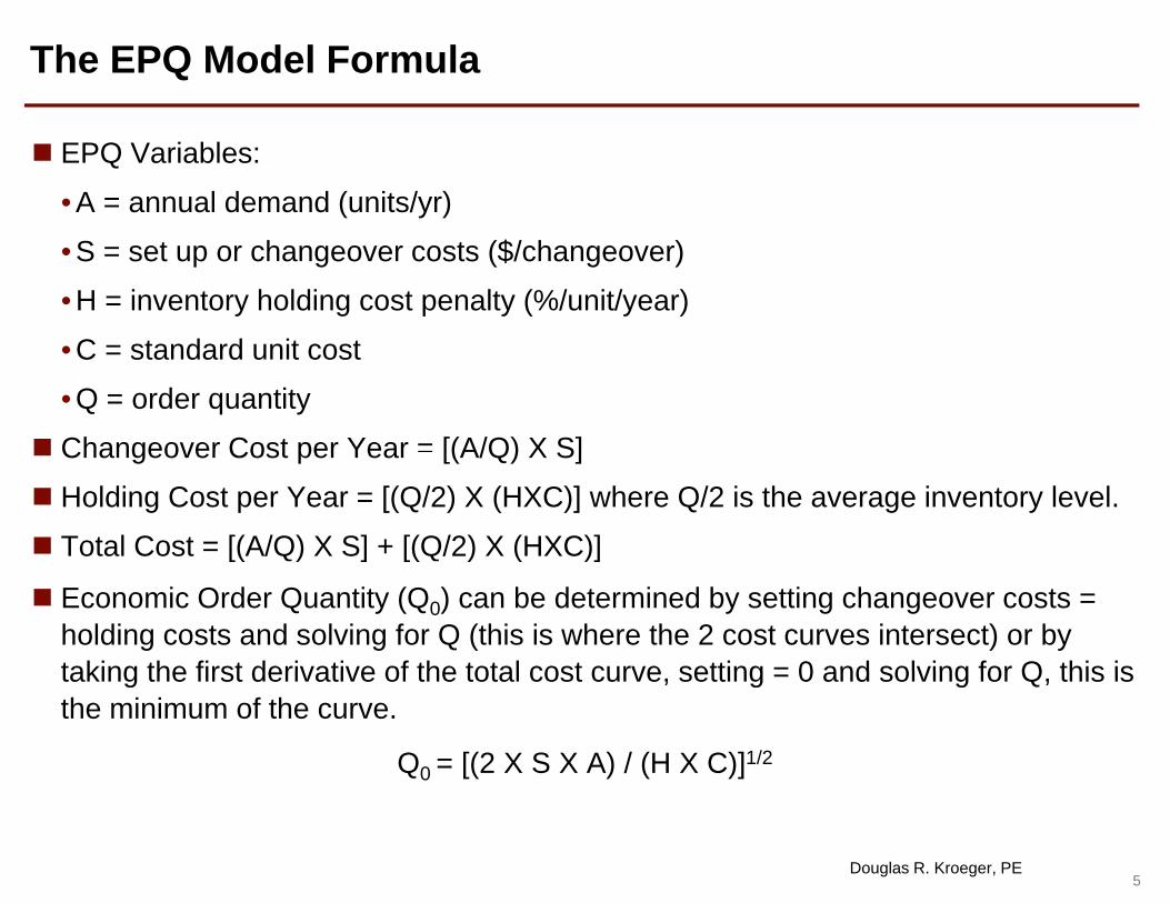
EPQ Variables:

• A = annual demand (units/yr)

• S = set up or changeover costs ($/changeover)

• H = inventory holding cost penalty (%/unit/year)

C t d d it t• C = standard unit cost

• Q = order quantity

Changeover Cost per Year = [(A/Q) X S]Changeover Cost per Year [(A/Q) X S]

Holding Cost per Year = [(Q/2) X (HXC)] where Q/2 is the average inventory level.

Total Cost = [(A/Q) X S] + [(Q/2) X (HXC)] [( ) ] [( ) ( )]

Economic Order Quantity (Q0) can be determined by setting changeover costs = holding costs and solving for Q (this is where the 2 cost curves intersect) or by taking the first derivative of the total cost curve setting = 0 and solving for Q this istaking the first derivative of the total cost curve, setting = 0 and solving for Q, this is the minimum of the curve.

Q0 = [(2 X S X A) / (H X C)]1/2


The EPQ Model Graph

$250,000

$200,000

TOT VAR COST

$150,000

L C

OST

HOLDING COST

TOT VAR COST

$120,000

$100,000TOTA

$50,000CO COST

$00 20,000 40,000 60,000 80,000 100,000 120,000 140,000 160,000

75,000 cases


ORDER QUANTITY (cases)

Sample Calculation: Q0 = [(2 X S X A) / (H X C)]1/2

EPQ Variables:

• A = annual demand (units/yr) = 3.0MM

• S = set up or changeover costs ($/changeover) = $10M

• H = inventory holding cost penalty (%/unit/year) = 21%

C t d d it t $5 00• C = standard unit cost = $5.00

Q0 = [(2 X S X A) / (H X C)]1/2 = 240,000 units/order

Order Cost per Year = [(A/Q) X S] = $125M

Holding Cost per Year = [(Q/2) X (HXC)] where Q/2 is the average inventory levelo d g Cost pe ea [(Q/ ) ( C)] e e Q/ s t e a e age e to y e e

= $125M

Total Cost = [(A/Q) X S] + [(Q/2) X H] = $250M


The EPQ Model (cont’d)

$1 200 000

$1,400,000

$1,000,000

$1,200,000

TCmin = $250,000/yr

$800,000Q0 = 240,000 units/order

$400 000

$600,000

$200,000

$400,000

HOLDING COST

TOT VAR COST

$00 100,000 200,000 300,000 400,000 500,000 600,000

CO COST


Getting Started / Gaining Alignment

Determine what factors effect the duration of a changeover – item last produced, item produced next or a combination

Identify how many changeover types there are in the process being studied e g :Identify how many changeover types there are in the process being studied, e.g.:

• Push – color change going from light to dark

• Simple – few raw materials used, not a lot of equipment to cleanS p e e a a e a s used, o a o o equ p e o c ea

• Complex – many raw materials used, a lot of equipment to clean

• Special Cases -hard to clean materials-packaging change vs. formula change vs. both-long runs = more cleaning

t f d ’t ll f tti ‘h d t t’ t l i f t d-nature of process doesn’t allow for getting a ‘head start’ at cleaning front end


Getting Started / Gaining Alignment (cont’d)

Establish what costs will be included in changeover costs:

• Labor – direct & indirect

• Variable overhead

• Cleaning chemicals and supplies

P d t t i i i k i• Product waste – in processing, in packaging

• Start-up costs

Determine how changeover costs will be quantifiedDetermine how changeover costs will be quantified

• Actual vs. standard – time, losses, crewing

• Product losses – material costs vs. variable costingg

• Start-up costs – labor and losses, need diligence to quantify

• Validate the numbers!


Getting Started / Gaining Alignment (cont’d)

Determine what will be included in holding costs:

• Finished good cost

Benefits and fixed overhead are included in the finished good cost portion of-Benefits and fixed overhead are included in the finished good cost portion of holding costs. Benefits and fixed overhead are excluded from the changeover costs. This is a standard EPQ procedure.

I t h ldi lt i t i ll d 21%• Inventory holding penalty is typically around 21%:-Cost of capital - 9%-Cost of obsolescence – 4%Actual warehousing cost 6%-Actual warehousing cost – 6%

-Cost of complexity/seasonality – 2%


Questions on The Basics


Understanding the Model - Changeover Costs Distribution

Changeover Cost Distribution Example

ChemicalStart Up (Wages &

VOH)23%

2% Filler Waste0%

Process Waste29%

Down Time (Wages & VOH)46%46%


Sensitivity Example – Changeover Costs Affect on EPQ

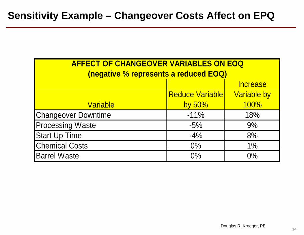
AFFECT OF CHANGEOVER VARIABLES ON EOQ

Increase

AFFECT OF CHANGEOVER VARIABLES ON EOQ(negative % represents a reduced EOQ)

VariableReduce Variable

by 50%Variable by

100%Changeover Downtime -11% 18%Changeover Downtime 11% 18%Processing Waste -5% 9%Start Up Time -4% 8%Chemical Costs 0% 1%Chemical Costs 0% 1%Barrel Waste 0% 0%


Sensitivity Example – The Flat Spot on the EPQ Curve

$250,000

A production quantitiy of +40%, -30% around the EPQ can be run ith onl a 6% nfa orable impact on total cost!

$200,000

TOT VAR COSTCHANGE IN TOTAL COST

with only a 6% unfavorable impact on total cost!

$150,000

AL

CO

ST

HOLDING COST

TOT VAR COSTCHANGE IN TOTAL COST

$100,000TOTA

$50,000CO COST

EPQ RANGE

$00 20,000 40,000 60,000 80,000 100,000 120,000 140,000 160,000

EPQ RANGE


ORDER QUANTITY (cases)

Sensitivity – The Flat Spot on the EPQ Curve

The total cost curve is relatively flat on either side of the EPQ.

This results in a very forgiving EPQ.

In the this case, for each SKU, the EPQ can vary up to +40%, -30% with only a 6% penalty in total cost.

Increasing the EPQ will increase inventory levels and increase holding costs whileIncreasing the EPQ will increase inventory levels and increase holding costs while decreasing changeover costs and decreasing utilization.

Decreasing the EPQ will decrease inventory levels and decrease holding costs while increasing changeover costs increasing utilization.

This is evident in data as well as the graph.


EPQ Effect on Capacity

On an annual basis, hours required per SKU can be divided into 3 categories:

• Changeover hours

• Start up hours• Start-up hours

• Run hours

A l hAnnual run hours

• Fixed

• Annual run hours required are equal to the units required divided by the expectedAnnual run hours required are equal to the units required divided by the expected units per hour

Annual start up and changeover hours

• Start up and changeover hours per occurrence are fixed, but the occurrences are dependant on the order quantity.

The lower the order quantity, the higher the occurrence of changeovers and start-q y g gups and the higher the total changeover and start-up hours required.

The higher the order quantity the lower the machine utilization and the higher the capacity.


p y

EPQ Hours Used Profile & Utilization

Hours Used Profile - EPQ(96% utilization)

TOTAL RUN TOTAL C/O DTTIME89%

TOTAL S/U DT

TOTAL C/O DT5%

AVAILABLE

TOTAL S/U DT 2%

AVAILABLE TIME4%


EPQ - Utilization Sensitivity Graph

X Coordinate times EOQ vs. % Utilization

150%

140%

150%

120%

130%

tion

At EPQ (1xEPQ) utilization is 96%

110%

% U

tiliz

at At EPQ (1xEPQ), utilization is 96%.

At the lower end of our range, .6XEPQ, utilization is 100%

At the upper end of our acceptable range, 1.3XEPQ, utilization is 94%

90%

100%At the upper end of our acceptable range, 1.3XEPQ, utilization is 94%

80%0 1 2 3 4 5 6 7 8 9 10


X time EPQ

Questions on Understanding the Model


The Case Study


The Case Study - Objectives

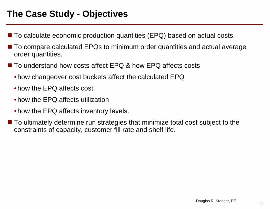
To calculate economic production quantities (EPQ) based on actual costs.

To compare calculated EPQs to minimum order quantities and actual average order quantitiesorder quantities.

To understand how costs affect EPQ & how EPQ affects costs

• how changeover cost buckets affect the calculated EPQo c a geo e cos buc e s a ec e ca cu a ed Q

• how the EPQ affects cost

• how the EPQ affects utilization

• how the EPQ affects inventory levels.

To ultimately determine run strategies that minimize total cost subject to the constraints of capacity customer fill rate and shelf lifeconstraints of capacity, customer fill rate and shelf life.


The Case Study

A production line had a utilization over 100%.

Customer orders were not being met, service level was low.

Minimum order quantities had been calculated in the past.

Actual average order quantities were below minimum order quantities.

The EPQ was compared to actual average run quantities and to the facility’s minimum production quantity.

The comparison showed that producing at the EPQs would result in a net savings.

Running calculated EPQs was not practical due to scheduling & other constraints.

A bl t t d l dA usable run strategy was developed.


Summary - EPQ vs Minimum PQ vs YTD Average PQ

Comparison - EPQ vs. Minimum PQ and EPQ vs. YTD Ave PQ3

C/O perAverage

C/O Cost Holding Total Cost A erage Average Inventory

(cs)

C/O per Year

gProduction Quantity1

C/O Cost per Year

gCost per

Yearper Year (C/O

& Holding)

Average WFC % Ute

( )EPQ vs. Minimum Order 35,000 -$413,000 $331,000 -$82,000 2.1 -38 4% 410,000

EPQ vs. YTD Ave Order 52,000 -$760,000 $485,000 -$275,000 2.9 -65 -3% 595,000

N t

, , , , ,

Notes: 1. Average Order Quantity is weighted by orders per year.2. Average WFC is a straight average over 27 SKUs.


g g g3. Negative numbers indicate a decrease if the EPQ quantity is used.

Positive numbers indicate an increase.

Run Strategy 1 – EPQ Runs, All SKUs

SKU GROUP DESCRIPTION ANNUAL

REQT'S (units)

EOQT

(frequency in weeks)

N (runs/year)

TOTAL TIME REQ'D (C/O + S/U + run)

FG ITEM #1 3,560,000 551,510 8.1 6.5 67FG ITEM #2 2,919,756 462,490 8.2 6.3 57FG ITEM #3 3,520,205 565,790 8.4 6.2 70FG ITEM #4 2,220,369 405,110 9.5 5.5 50FG ITEM #5 2,311,231 425,050 9.6 5.4 53FG ITEM #6 3,372,191 623,200 9.6 5.4 77FG ITEM #7 2,592,466 543,580 10.9 4.8 68FG ITEM #8 2,584,143 553,740 11.1 4.7 69

A (Size 1)

Total Hrs 510Total Wks 3.0

FG ITEM #9 899,393 219,310 12.7 4.1 27FG ITEM #10 1,789,282 437,590 12.7 4.1 55FG ITEM #11 2,049,585 503,990 12.8 4.1 64FG ITEM #12 716,525 187,500 13.6 3.8 24BFG ITEM #13 808,199 212,920 13.7 3.8 26FG ITEM #14 765,024 205,000 13.9 3.7 26FG ITEM #15 548,607 162,830 15.4 3.4 21FG ITEM #16 500,622 169,060 17.6 3.0 21FG ITEM #17 481,479 163,730 17.7 2.9 21


B (Size 1)

FG ITEM #18 5,291,405 648,720 6.4 8.2 78FG ITEM #19 5,443,472 717,140 6.9 7.6 87FG ITEM #20 3,950,128 534,450 7.0 7.4 65FG ITEM #21 2,613,426 419,900 8.4 6.2 53FG ITEM #22 3,510,930 585,850 8.7 6.0 72FG ITEM #23 3,686,244 647,350 9.1 5.7 80

T t l H

C (Size 2)


FG ITEM #24 2,906,550 576,380 10.3 5.0 72FG ITEM #25 2,005,704 416,390 10.8 4.8 52FG ITEM #26 1,668,921 362,920 11.3 4.6 46FG ITEM #27 697,902 173,130 12.9 4.0 22

T t l H 193

D (Size 2)



`

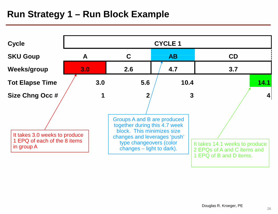
Run Strategy 1 – Run Block Example

Cycle

SKU G

CYCLE 1

CA AB CDSKU Goup

Weeks/group

T t El Ti 3 0

CA AB CD

3.0 2.6 4.7 3.7

10 45 6 14 1Tot Elapse Time 3.0

Size Chng Occ # 1 2 3 4

10.45.6 14.1

It t k 3 0 k t d

Groups A and B are produced together during this 4.7 week block. This minimizes size

It takes 3.0 weeks to produce 1 EPQ of each of the 8 items in group A

changes and leverages ‘push’ type changeovers (color changes – light to dark).

It takes 14.1 weeks to produce 2 EPQs of A and C items and 1 EPQ of B and D items.


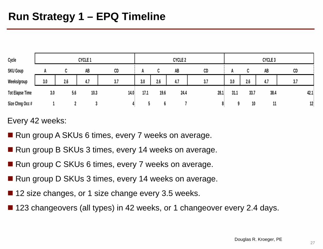
Run Strategy 1 – EPQ Timeline

Cycle CYCLE 1 CYCLE 2 CYCLE 3

SKU Goup

Weeks/group

Tot Elapse Time 3.0

C

17.1 31.1

A

4.7 3.7

AB CDCA AB CD

3.0 2.6

CDAB A C

3.0 2.6 4.7 3.73.0 2.6 4.7 3.7

5.6 42.138.433.714.0 28.119.610.3 24.4Tot Elapse Time 3.0

Size Chng Occ # 1 2 3 4 5 6 7 8 9 10 11 12

17.1 31.15.6 42.138.433.714.0 28.119.610.3 24.4

Every 42 weeks:y

Run group A SKUs 6 times, every 7 weeks on average.

Run group B SKUs 3 times, every 14 weeks on average.

Run group C SKUs 6 times, every 7 weeks on average.

Run group D SKUs 3 times, every 14 weeks on average.

12 size changes, or 1 size change every 3.5 weeks.

123 changeovers (all types) in 42 weeks, or 1 changeover every 2.4 days.


Run Strategy 1 – EPQ Run Frequency & Slack Time


REQT'S (A)

EOQT

(freq In

AVEFREQ

"PAD" AVE F

REQ T(A) (units)

Inweeks)

Q REQ - T

FG ITEM #9 389,737 95,031 12.7 14.0 -1.4,FG ITEM #10 775,355 189,622 12.7 14.0 -1.3FG ITEM #11 888,154 218,392 12.8 14.0 -1.3FG ITEM #12 310,494 81,250 13.6 14.0 -0.4BFG ITEM #13 350,220 92,263 13.7 14.0 -0.3FG ITEM #14 331,510 88,831 13.9 14.0 -0.1FG ITEM #15 237,730 70,557 15.4 14.0 1.4

B (Sz1)

FG ITEM #16 216,936 73,256 17.6 14.0 3.5FG ITEM #17 208,641 70,947 17.7 14.0 3.6


Run Strategy 1 – EPQ Run Frequency & Slack Time


REQT'S (units)

EOQT

(frequency in weeks)

N (runs/year)

TOTAL TIME REQ'D (S/U + run + C/O)

FREQUENCY 1

FREQUENCY 2

AVE FREQ

"PAD" AVE FREQ - T

FG ITEM #1 3,560,000 551,510 8.1 6.5 67 5.6 8.5 7.1 1.0FG ITEM #2 2,919,756 462,490 8.2 6.3 57 5.6 8.5 7.1 1.2FG ITEM #3 3,520,205 565,790 8.4 6.2 70 5.6 8.5 7.1 1.3FG ITEM #4 2,220,369 405,110 9.5 5.5 50 5.6 8.5 7.1 2.4FG ITEM #5 2,311,231 425,050 9.6 5.4 53 5.6 8.5 7.1 2.5FG ITEM #6 3,372,191 623,200 9.6 5.4 77 5.6 8.5 7.1 2.6FG ITEM #7 2,592,466 543,580 10.9 4.8 68 5.6 8.5 7.1 3.9FG ITEM #8 2,584,143 553,740 11.1 4.7 69 5.6 8.5 7.1 4.1

A(Size 1)


FG ITEM #9 899,393 219,310 12.7 4.1 27 14.1 14.1 14.1 (1.4)FG ITEM #10 1,789,282 437,590 12.7 4.1 55 14.1 14.1 14.1 (1.4)FG ITEM #11 2,049,585 503,990 12.8 4.1 64 14.1 14.1 14.1 (1.3)FG ITEM #12 716,525 187,500 13.6 3.8 24 14.1 14.1 14.1 (0.5)B FG ITEM #13 808,199 212,920 13.7 3.8 26 14.1 14.1 14.1 (0.4)FG ITEM #14 765,024 205,000 13.9 3.7 26 14.1 14.1 14.1 (0.2)FG ITEM #15 548,607 162,830 15.4 3.4 21 14.1 14.1 14.1 1.3FG ITEM #16 500,622 169,060 17.6 3.0 21 14.1 14.1 14.1 3.5FG ITEM #17 481,479 163,730 17.7 2.9 21 14.1 14.1 14.1 3.6


B (Size 1)

FG ITEM #18 5,291,405 648,720 6.4 8.2 78 7.3 6.8 7.1 (0.7)FG ITEM #19 5,443,472 717,140 6.9 7.6 87 7.3 6.8 7.1 (0.2)FG ITEM #20 3,950,128 534,450 7.0 7.4 65 7.3 6.8 7.1 (0.0)FG ITEM #21 2,613,426 419,900 8.4 6.2 53 7.3 6.8 7.1 1.3FG ITEM #22 3,510,930 585,850 8.7 6.0 72 7.3 6.8 7.1 1.6FG ITEM #23 3,686,244 647,350 9.1 5.7 80 7.3 6.8 7.1 2.1

C (Size 2)

FG ITEM #23 3,686,244 647,350 9.1 5.7 80 7.3 6.8 7.1 2.1Total Hrs 435

Total Wks 2.6

FG ITEM #24 2,906,550 576,380 10.3 5.0 72 14.1 14.1 14.1 (3.8)FG ITEM #25 2,005,704 416,390 10.8 4.8 52 14.1 14.1 14.1 (3.3)FG ITEM #26 1,668,921 362,920 11.3 4.6 46 14.1 14.1 14.1 (2.8)FG ITEM #27 697 902 173 130 12 9 4 0 22 14 1 14 1 14 1 (1 2)

D (Size 2)


FG ITEM #27 697,902 173,130 12.9 4.0 22 14.1 14.1 14.1 (1.2)Total Hrs 193 # SKUs w/ Negative Slack 11

Total Wks 1.1 # SKUs w/ Positive Slack 16Minimum Slack -4.5

` Maximum Slack 4.1

Run Strategy 2 – Adjusted Run Quantities

Condition Meaning Options Actions- SKU needed before scheduled Make more Increase OQ

Slack Weeks

- SKU needed before scheduled Make more Increase OQ(Making it late) Make sooner Decrease other OQ

+ SKU d d ft h d l d M k l D OQ+ SKU needed after scheduled Make less Decrease OQ(Making it early) Make later Increase other OQ

Hybrid run strategies were developed by increasing or decreasing order quantity based on the condition of the ‘Slack’ weeks.

Several iterations were performed varying the order quantity while monitoring the time between runs and the slack weeks.

The objective was to eliminate/minimize negative slack while minimizing time between runs.


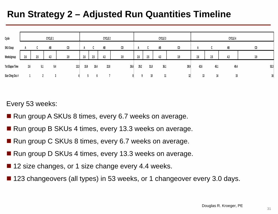
Run Strategy 2 – Adjusted Run Quantities Timeline

Cycle

SKU Goup AB CD AA C

CYCLE 3

A C AB CD

CYCLE 4

C AB CD

CYCLE 1 CYCLE 2

C AB CDA

Weeks/group

Tot Elapse Time 2.6

Size Chng Occ # 1 2 3 4 5 6 7 8 9 10 11 12 13 14 15 16

15.9 29.2 42.6

2.6 2.5

26.6

3.9 4.32.6 2.5 4.3 2.6 2.5 4.3 3.9

31.8 36.1 39.9

2.6 2.5 4.3 3.9

45.1 49.4 53.3

3.9

5.1 9.4 13.3 18.4 22.8

Every 53 weeks:y

Run group A SKUs 8 times, every 6.7 weeks on average.

Run group B SKUs 4 times, every 13.3 weeks on average.

Run group C SKUs 8 times, every 6.7 weeks on average.

Run group D SKUs 4 times, every 13.3 weeks on average.

12 size changes, or 1 size change every 4.4 weeks.

123 changeovers (all types) in 53 weeks, or 1 changeover every 3.0 days.


Run Strategy 2 – Adjusted Run Quantities & Slack Time

SKU GROUP DESCRIPTION

2008 ANNUAL REQT'S (units)

Adjusted Production

Quantity

Total Time Req'd (S/U

+ Run + C/O)

Freq 1 Freq 2 Ave Freq

Reqd Freq

"SLACK" (AVE FREQ -

T)

FG ITEM #1 3,560,000 468,801 58 5.3 8.3 6.8 6.9 0.0G #FG ITEM #2 2,919,756 131,044 49 5.3 8.3 6.8 7.0 0.2

FG ITEM #3 3,520,205 160,313 60 5.3 8.3 6.8 7.1 0.3FG ITEM #4 2,220,369 114,785 43 5.3 8.3 6.8 8.1 1.2FG ITEM #5 2,311,231 120,435 46 5.3 8.3 6.8 8.1 1.3FG ITEM #6 3,372,191 176,580 66 5.3 8.3 6.8 8.2 1.3FG ITEM #7 2,592,466 154,020 58 5.3 8.3 6.8 9.3 2.4FG ITEM #8 2,584,143 156,899 59 5.3 8.3 6.8 9.5 2.6

T t l H 439

A (Size 1)


FG ITEM #9 899,393 263,186 93 13.6 13.6 13.6 15.2 1.6FG ITEM #10 1,789,282 525,135 186 13.6 13.6 13.6 15.3 1.6FG ITEM #11 2,049,585 604,820 215 13.6 13.6 13.6 15.3 1.7FG ITEM #12 716,525 225,012 80 13.6 13.6 13.6 16.3 2.7FG ITEM #13 808 199 255 517 90 13 6 13 6 13 6 16 4 2 8

B FG ITEM #13 808,199 255,517 90 13.6 13.6 13.6 16.4 2.8FG ITEM #14 765,024 246,013 87 13.6 13.6 13.6 16.7 3.1FG ITEM #15 548,607 138,411 50 13.6 13.6 13.6 13.1 -0.5FG ITEM #16 500,622 143,706 52 13.6 13.6 13.6 14.9 1.3FG ITEM #17 481,479 139,176 50 13.6 13.6 13.6 15.0 1.4


(Size 1)

FG ITEM #18 5,291,405 778,505 272 7.0 6.7 6.8 7.7 0.8FG ITEM #19 5,443,472 860,613 301 7.0 6.7 6.8 8.2 1.4FG ITEM #20 3,950,128 641,374 225 7.0 6.7 6.8 8.4 1.6FG ITEM #21 2,613,426 356,928 128 7.0 6.7 6.8 7.1 0.3FG ITEM #22 3,510,930 497,991 177 7.0 6.7 6.8 7.4 0.6FG ITEM #23 3,686,244 550,268 195 7.0 6.7 6.8 7.8 0.9

T t l H 1 298

C (Size 2)

Total Hrs 1,298Total Wks 7.7

FG ITEM #24 2,906,550 691,692 245 13.6 13.6 13.6 12.4 -1.3FG ITEM #25 2,005,704 499,694 177 13.6 13.6 13.6 13.0 -0.7FG ITEM #26 1,668,921 435,527 155 13.6 13.6 13.6 13.6 -0.1FG ITEM #27 697,902 207,767 74 13.6 13.6 13.6 15.5 1.8

T t l H 650 # SKU / N ti Sl k 4

D (Size 2)


Total Hrs 650 # SKUs w/ Negative Slack 4Total Wks 3.9 # SKUs w/ Positive Slack 23

Minimum Slack -1.3Maximum Slack 3.1

Summary – Adjusted OQ vs Min OQ vs YTD Average OQ

Comparison - EPQ vs. Minimum Order Quantity and EPQ vs. YTD Ave Order Qty3

Average I t

Average WFC2

C/O per Y % Ute

Average Productio C/O Cost

Y

Holding Cost per

Total Cost per Year (C/O & Inventory

(cs)Adjusted Production Qty vs. Min Production Qty 14,712 -$247,692 $155,804 -$91,888 0.6 -19 4.4% 191,067

WFC2 Yearn Quantity

per Year pYear (C/O &

Holding)

Adjusted Production Qty vs. YTD Ave Production Qty 31,327 -$594,659 $310,194 -$284,464 1.3 -45 -2.5% 376,531

Notes: 1. Average Order Quantity is weighted by orders per year.2 Average WFC is a straight average over 27 SKUs2. Average WFC is a straight average over 27 SKUs. 3. Negative numbers indicate a decrease if the EPQ quantity is used.

Positive numbers indicate an increase.


Final Steps

Several iterations were performed to determine acceptable production quantities (within +40%,-30% of EPQ) for each Finished Good Item that resulted in no negative slack.

These production quantities were used in the actual plant finite scheduling model which accounts for actual schedule downtime, consumption, inventory levels, raw and packaging material availability etc.

After determining that EPQs do work when considering all ‘real life’ variables, an implementation plan was developed.

Implementation plan included phasing in acceptable EPQ quantities as production schedules were developed.


QUESTIONS?

Douglas R. Kroeger, PE

Contact information available through IIE membership directory.


Date post:	03-Apr-2020
Category:	Documents
Upload:	others
View:	1 times
Download:	0 times

Determining Economic Production Quantities Webinar July 14 ... Economic... · To calculate economic...

Documents