DETERMINING THE FATE AND TRANSPORT OF THE ACRYLAMIDE MONOMER (AMD) IN SOIL AND GROUNDWATER SYSTEMS by Todd James Arrowood Bachelor of Science in Geology University of Nevada, Las Vegas 2005 A thesis submitted in partial fulfillment of the requirements for the Master of Science Degree in Geoscience Department of Geoscience College of Sciences Graduate College University of Nevada, Las Vegas May 2008
Transcript
DETERMINING THE FATE AND TRANSPORT OF THE ACRYLAMIDE
MONOMER (AMD) IN SOIL AND GROUNDWATER SYSTEMS
by
Todd James Arrowood
Bachelor of Science in Geology University of Nevada, Las Vegas
2005
A thesis submitted in partial fulfillment
of the requirements for the
Master of Science Degree in Geoscience Department of Geoscience
College of Sciences
Graduate College University of Nevada, Las Vegas
May 2008
ii
(Approval Page)
iii
ABSTRACT
Determining the Fate and Transport of the Acrylamide Monomer (AMD) in Soil
and Groundwater Systems
by
Todd James Arrowood
Dr. Zhongbo Yu, Examination Committee Chair Associate Professor of Hydrogeology
University of Nevada, Las Vegas
Dr. Michael H. Young, Examination Committee Co-Chair Associate Research Professor, Division of Hydrologic Sciences
Desert Research Institute (DRI)
Acrylamide (AMD) is a known animal and suspected human carcinogen and is used
to produce polyacrylamide (PAM), which has been proposed as a technology for seepage
control in unlined water delivery canals. Previous studies have not quantified the fate and
transport of AMD in soil and groundwater systems. In this study, batch experiments and
soil column tests (with and without microbial degradation) were conducted on three
materials (control sand, gravelly sand and loam soil) to determine the Kd, retardation
factor, the form of the sorption isotherm, and determine microbial degradation rates. Soil
core tests from samples collected in canals were also conducted to simulate field-scale
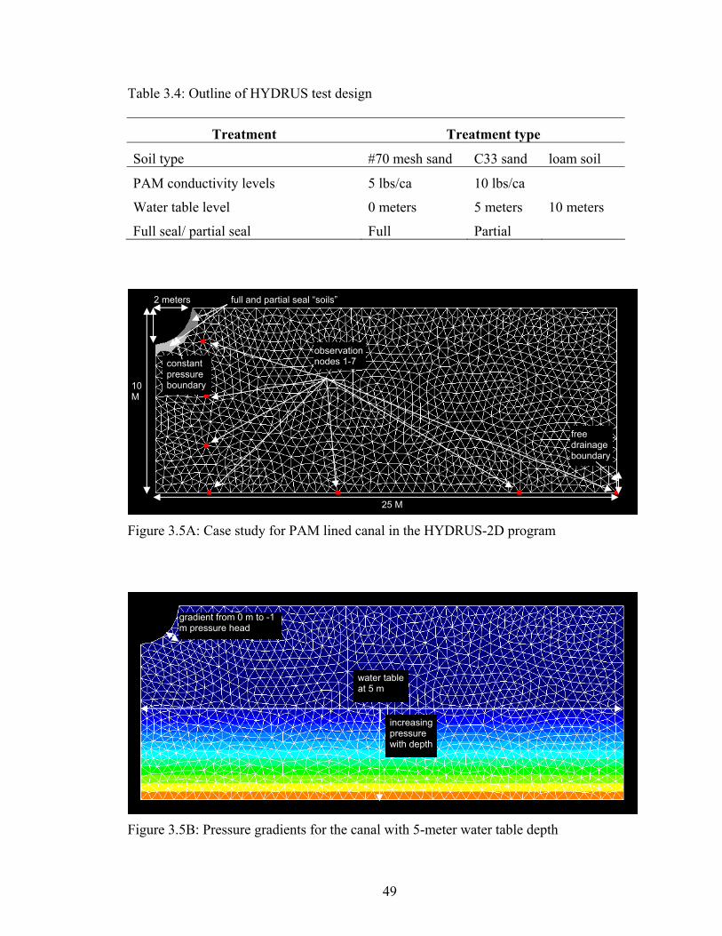
transport. A numerical model (HYDRUS-2D) was used to simulate a canal environment
using the fate and transport parameters of AMD obtained in the laboratory. Results
indicate a Freundlich-type sorption isotherm for AMD in the loam soil and a linear
iv
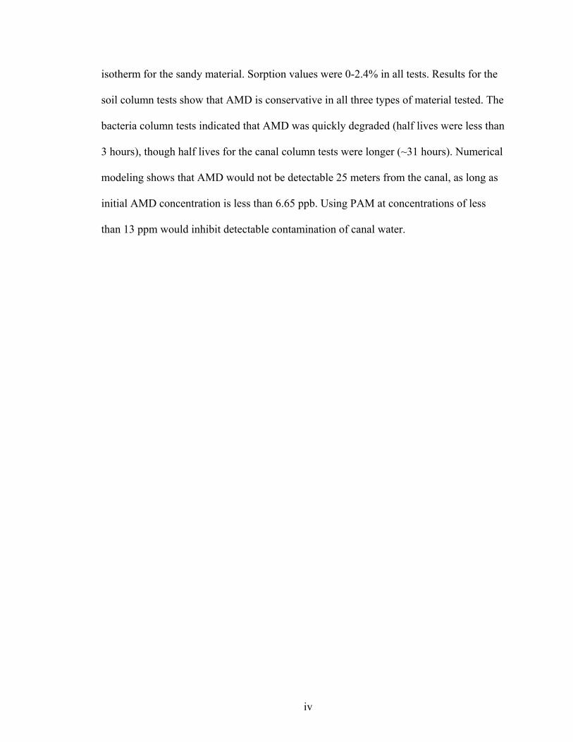
isotherm for the sandy material. Sorption values were 0-2.4% in all tests. Results for the
soil column tests show that AMD is conservative in all three types of material tested. The
bacteria column tests indicated that AMD was quickly degraded (half lives were less than
3 hours), though half lives for the canal column tests were longer (~31 hours). Numerical
modeling shows that AMD would not be detectable 25 meters from the canal, as long as
initial AMD concentration is less than 6.65 ppb. Using PAM at concentrations of less
than 13 ppm would inhibit detectable contamination of canal water.
v
TABLE OF CONTENTS ABSTRACT……............................................................................................................... iii TABLE OF CONTENTS.....................................................................................................v LIST OF FIGURES .......................................................................................................... vii LIST OF TABLES........................................................................................................... viii ACKNOWLEDGEMENTS............................................................................................... ix CHAPTER 1 INTRODUCTION ........................................................................................1 CHAPTER 2 LITERATURE REVIEW .............................................................................8
2.1 Previous agricultural PAM usage ............................................................................. 8 2.2 Possible PAM breakdown to AMD ........................................................................ 10 2.3 PAM and AMD transport........................................................................................ 13 2.4 AMD microbial breakdown .................................................................................... 16
CHAPTER 3 MATERIALS, METHODOLOGY, AND DATA DESCRIPTION...........20
3.1 Description of soil material..................................................................................... 20 3.2 HPLC chemical analysis ......................................................................................... 22 3.3 Experiment 1: AMD sorption batch tests................................................................ 23
3.6.1.1 Test solution for column tests ................................................................... 44 3.6.1.2 Isolation and characterization of column test bacterium .......................... 44
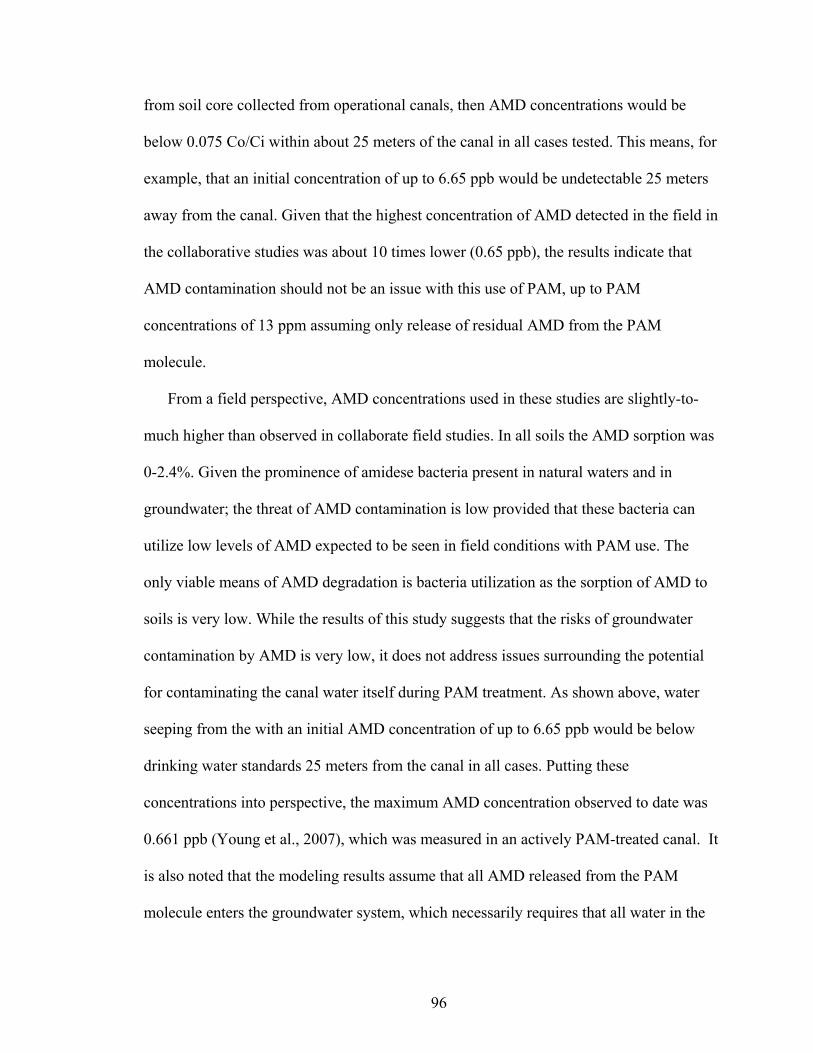
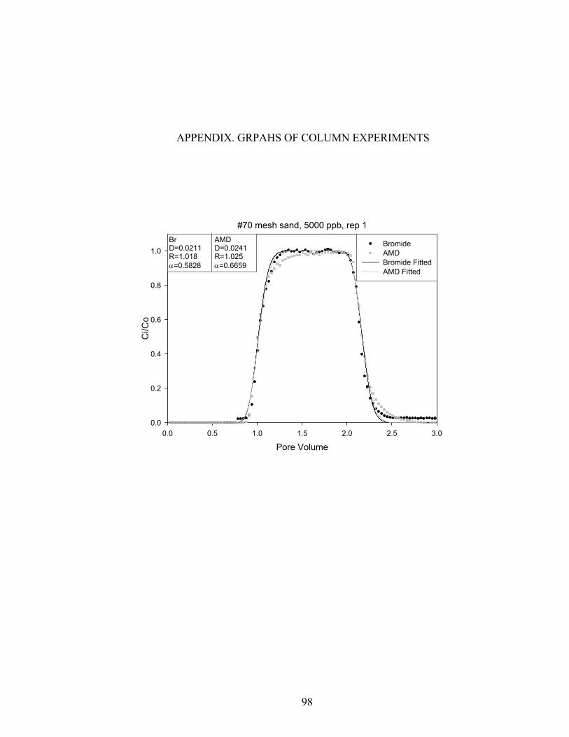
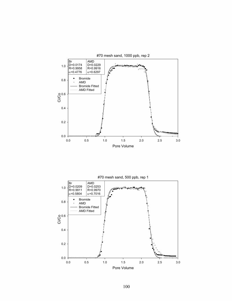
4.7 Results for the predictive numerical modeling with HYDRUS-2D ....................... 84 CHAPTER 5 CONCLUSIONS AND RECOMMENDATIONS.....................................94 APPENDIX. GRPAHS OF COLUMN EXPERIMENTS.................................................98 REFERENCES… ............................................................................................................114 VITA………….. ..............................................................................................................123
vii
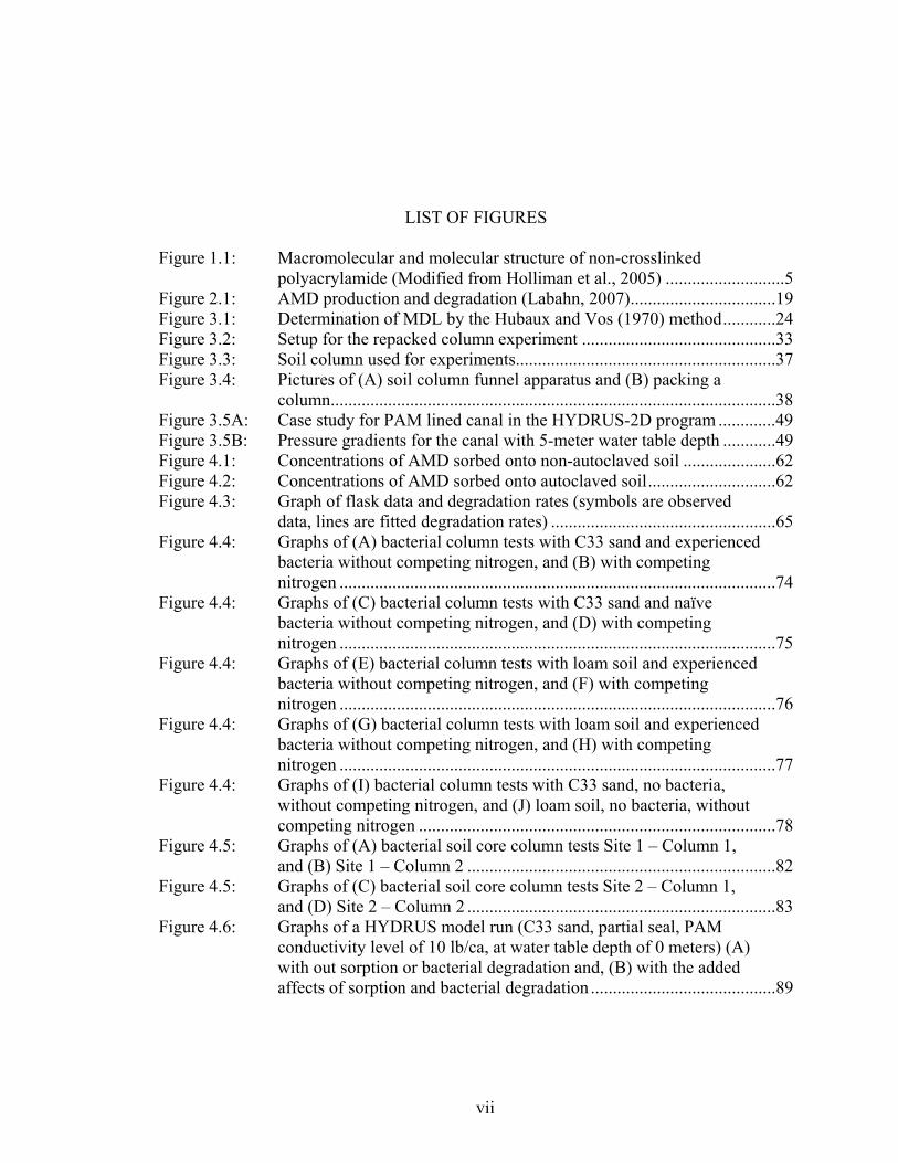
LIST OF FIGURES
Figure 1.1: Macromolecular and molecular structure of non-crosslinked polyacrylamide (Modified from Holliman et al., 2005) ...........................5 Figure 2.1: AMD production and degradation (Labahn, 2007).................................19 Figure 3.1: Determination of MDL by the Hubaux and Vos (1970) method............24 Figure 3.2: Setup for the repacked column experiment ............................................33 Figure 3.3: Soil column used for experiments...........................................................37 Figure 3.4: Pictures of (A) soil column funnel apparatus and (B) packing a column.....................................................................................................38 Figure 3.5A: Case study for PAM lined canal in the HYDRUS-2D program .............49 Figure 3.5B: Pressure gradients for the canal with 5-meter water table depth ............49 Figure 4.1: Concentrations of AMD sorbed onto non-autoclaved soil .....................62 Figure 4.2: Concentrations of AMD sorbed onto autoclaved soil.............................62 Figure 4.3: Graph of flask data and degradation rates (symbols are observed data, lines are fitted degradation rates) ...................................................65 Figure 4.4: Graphs of (A) bacterial column tests with C33 sand and experienced bacteria without competing nitrogen, and (B) with competing nitrogen ...................................................................................................74 Figure 4.4: Graphs of (C) bacterial column tests with C33 sand and naïve bacteria without competing nitrogen, and (D) with competing nitrogen ...................................................................................................75 Figure 4.4: Graphs of (E) bacterial column tests with loam soil and experienced bacteria without competing nitrogen, and (F) with competing nitrogen ...................................................................................................76 Figure 4.4: Graphs of (G) bacterial column tests with loam soil and experienced bacteria without competing nitrogen, and (H) with competing nitrogen ...................................................................................................77 Figure 4.4: Graphs of (I) bacterial column tests with C33 sand, no bacteria, without competing nitrogen, and (J) loam soil, no bacteria, without competing nitrogen .................................................................................78 Figure 4.5: Graphs of (A) bacterial soil core column tests Site 1 – Column 1, and (B) Site 1 – Column 2 ......................................................................82 Figure 4.5: Graphs of (C) bacterial soil core column tests Site 2 – Column 1, and (D) Site 2 – Column 2 ......................................................................83 Figure 4.6: Graphs of a HYDRUS model run (C33 sand, partial seal, PAM conductivity level of 10 lb/ca, at water table depth of 0 meters) (A) with out sorption or bacterial degradation and, (B) with the added affects of sorption and bacterial degradation ..........................................89
viii
LIST OF TABLES
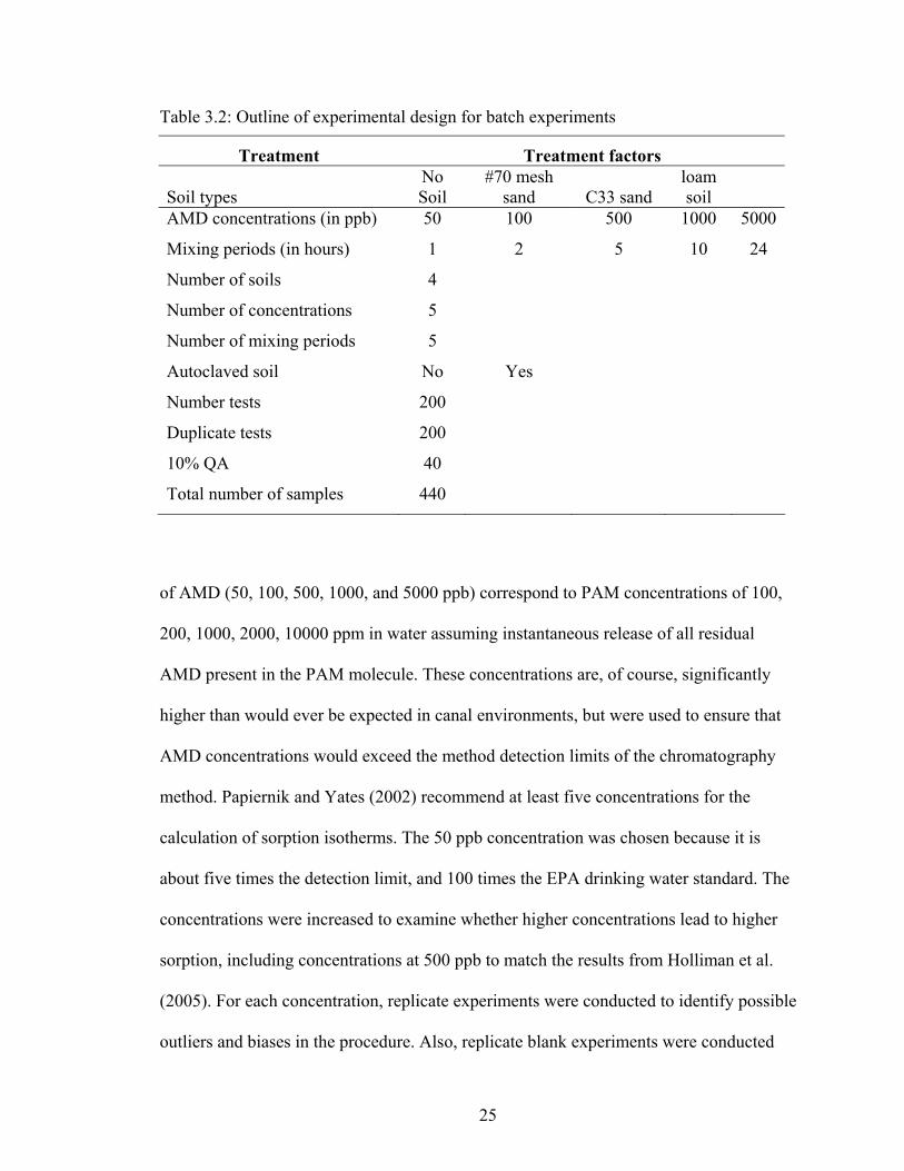
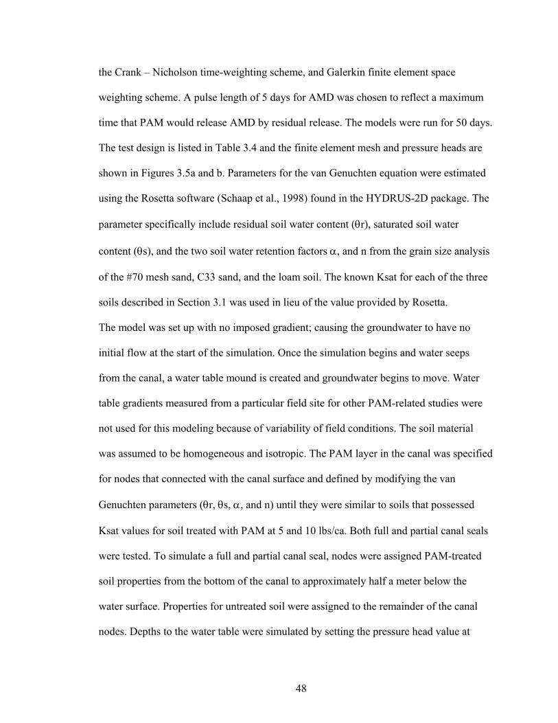
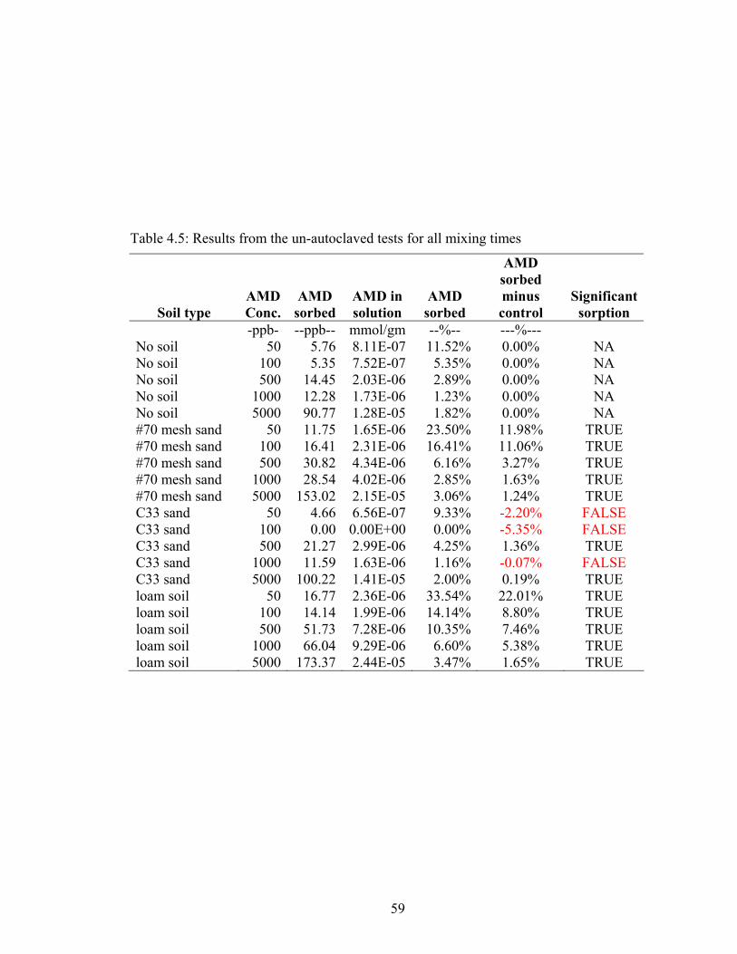
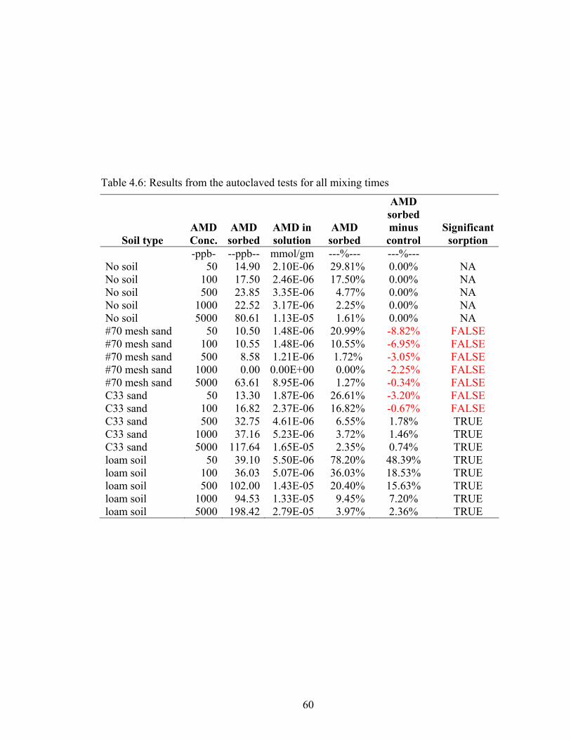
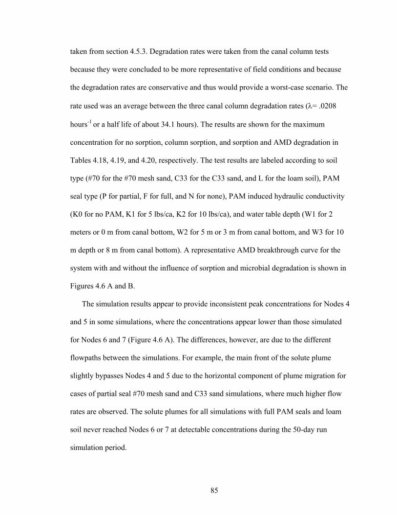
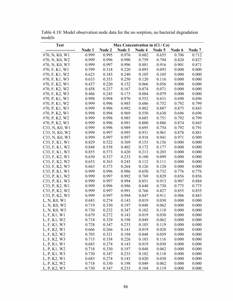
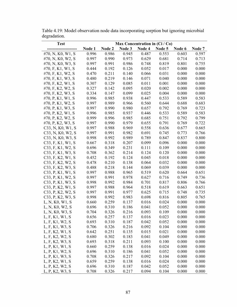
Table 1.1: Chemical and physical properties of acrylamide ......................................4 Table 3.1: Critical level and minimum detection limit for all experiments .............24 Table 3.2: Outline of experimental design for batch experiments ...........................25 Table 3.3: General setup for bromide/AMD column tests.......................................33 Table 3.4: Outline of HYDRUS test design.............................................................49 Table 3.5: Observation node properties ...................................................................51 Table 4.1: Particle size distributions of fine-earth fraction (< 2 mm) for three soil materials used in the research. .........................................................56 Table 4.2: Particle size analysis for C33 sand and loam soil autoclaved samples...56 Table 4.3: Change in grain size for C33 sand and loam from autoclaving cycles...57 Table 4.4: Surface area analysis...............................................................................57 Table 4.5: Results from the un-autoclaved tests for all mixing times......................59 Table 4.6: Results from the autoclaved tests for all mixing times ...........................60 Table 4.7: Correlation coefficients for isotherms ....................................................63 Table 4.8: Estimated retardation values ...................................................................63 Table 4.9: Estimated flask degradation values.........................................................65 Table 4.10: Recovery and experimental conditions for soil column experiments .....68 Table 4.11: Estimated transport parameters for the soil column test.........................69 Table 4.12: ANOVA and ANCOVA statistics for AMD parameter comparisons ....71 Table 4.13: Multiple comparison statistics for parameter comparisons ....................71 Table 4.14: Correlation coefficients for isotherms ....................................................73 Table 4.15: Degradation parameters for bacterial column tests.................................79 Table 4.16: Results of ANOVA analyses for parameter comparisons.......................80 Table 4.17: Degradation parameters for bacterial column tests.................................84 Table 4.18: Model observation node data for the no sorption, no bacterial degradation models .................................................................................86 Table 4.19: Model observation node data incorporating sorption but ignoring microbial degradation. ............................................................................87 Table 4.20: Model observation node data, including processes of sorption and bacterial degradation models ..................................................................88 Table 4.21: Arrival times of peak concentrations with no treatment and a partial seal for #70 mesh and C33 sand .............................................................91 Table 4.22: Arrival times of peak concentration with no treatment and a partial seal for #70 mesh and C33 sand, including microbial degradation of AMD .......................................................................................................91
ix
ACKNOWLEDGEMENTS
I would like to thank: The US Bureau of Reclamation for providing the funding to conduct PAM and
AMD research under cooperative agreement #04-FC-81-1064. Dr. Michael H. Young for giving me the opportunity to work on this project,
providing me with a graduate research assistantship and for so much advice and support in helping me finish this project.
Dr. Zhongbo Yu and all his help along the way in my undergraduate and graduate
work with feedback reviews, education, and all the help with computer modeling. My committee members Dr. Dave Kreamer and Dr. Thomas Piechota for the
feedback they provided and taking the time and effort to review this document. PAM peer review committee for constructive feedback
Dr. Duane Moser for helping me understand the small, vast world of
microbiology and bacteria and all the feedback. Ernesto Moran for helping me in the lab and giving me so much feedback, help,
equipment, training, and memories. Stephanie Labahn for all the help and assistance with experiments, setup, and the
knowledge of microbiology. John Goreham and Dr. Darren Meadows for teaching me so much in the lab and
keeping my spirits up. Jennifer Barth, Karen Levy, Christina Jacovides, Journet Wallace, for their help.
Jim Woodrow and Dr. Glenn Miller for their help in getting me familiar with
HPLC and their input and feedback for this project. All UNLV Geoscience Faculty and Staff and all the wonderful students and
researchers at UNLV and DRI who were such a big part of my life these last few years.
My parents for all their love and support
1
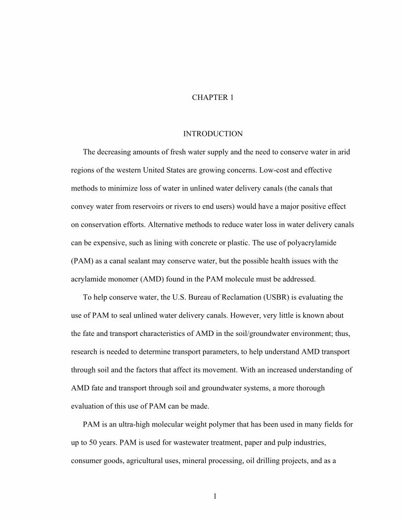
CHAPTER 1
INTRODUCTION
The decreasing amounts of fresh water supply and the need to conserve water in arid
regions of the western United States are growing concerns. Low-cost and effective
methods to minimize loss of water in unlined water delivery canals (the canals that
convey water from reservoirs or rivers to end users) would have a major positive effect
on conservation efforts. Alternative methods to reduce water loss in water delivery canals
can be expensive, such as lining with concrete or plastic. The use of polyacrylamide
(PAM) as a canal sealant may conserve water, but the possible health issues with the
acrylamide monomer (AMD) found in the PAM molecule must be addressed.
To help conserve water, the U.S. Bureau of Reclamation (USBR) is evaluating the
use of PAM to seal unlined water delivery canals. However, very little is known about
the fate and transport characteristics of AMD in the soil/groundwater environment; thus,
research is needed to determine transport parameters, to help understand AMD transport
through soil and the factors that affect its movement. With an increased understanding of
AMD fate and transport through soil and groundwater systems, a more thorough
evaluation of this use of PAM can be made.
PAM is an ultra-high molecular weight polymer that has been used in many fields for
up to 50 years. PAM is used for wastewater treatment, paper and pulp industries,
consumer goods, agricultural uses, mineral processing, oil drilling projects, and as a
2
water well and sewer pipe line sealant (EPA, 1994a; European Union Risk Assessment,
2002). In agriculture, PAM is currently used to stabilize soil structure in agricultural
irrigation furrow, causing more uniform infiltration and limiting soil erosion (Sojka and
Lentz, 1994; Spofford and Pfeiffer, 1996). The proposed new use of PAM as a canal
sealant is based on research showing that higher concentrations of PAM can decrease
infiltration in soil (Malik and Letey, 1992; Nadler et al., 1994; Letey, 1996; Lentz, 2003;
Ajwa and Trout, 2006).
PAM is formed through a polymerization process which takes millions of AMD
molecules and chains them together to make a single molecule of PAM. Many forms of
PAM exist. Linear anionic PAM is generally used in agriculture. This form is made with
acrylic acid so it is anionic or has a slight positive charge. In the production of PAM,
0.025 % to 0.05 % of residual AMD is left in the PAM molecule (Sojka et al., 1998a).
Therefore, if the PAM is added to the canal water at concentrations of 1 ppm, then the
AMD concentration released from the hydrated PAM molecule should not exceed 0.5
ppb, or the current EPA maximum concentration limit. Research has shown that PAM
itself has a low level of human toxicity (Lentz et al., 2002; Smith et al., 1996).
The AMD monomer used in the production of PAM is known to be a human
neurotoxin and is believed to be a human carcinogen, causing damage to cells on the
DNA level. AMD is already a known animal carcinogen and neurotoxin (EPA, 1994a and
b). EPA reported that exposures to humans have been associated with polyneuropathy
with motor and sensory impairment marked by numbness, paresthesias, ataxia, tremor,
dysarthria, and mid-brain lesions. Ingestion of contaminated drinking water has caused
drowsiness, disturbances of balance, confusion, memory loss, and hallucinations (EPA,
3
1994b). The current standard for AMD in water is 0.5 ppb and 0.25 ppb in the United
States and Europe, respectively (EPA, 1994b; European Union Risk Assessment, 2002).
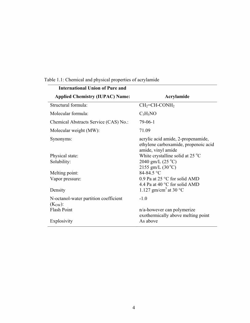
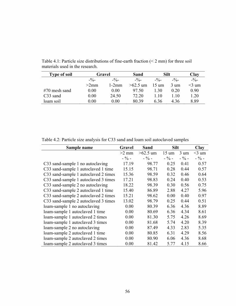
Chemical and physical properties of acrylamide are summarized below in Table 1.1
(European Union Risk Assessment, 2002). Acrylamide is solid at room temperature,
highly soluble in water, has a low potential to partition to organic matter, and has a low
volatilization potential in water.
When PAM hydrates, it expands and forms a random coiled structure (Figure 1.1) and
then moves with the water, attaches to suspended particles and sinks to the bottom of
channel. It then adheres to the soil on the bottom of the canal by forces of electrostatic,
hydrogen and chemical bonding (Lentz et al., 2002). The residual AMD in the PAM
molecule can be released from the PAM molecule in different areas of the canal. First,
the AMD molecule may be released when PAM is initially saturated; second, AMD may
be released after PAM has settled to the canal surface and is sealing the canal; and third
AMD may be released if PAM is transported into the subsurface of the canal, though
research has shown that PAM transport beyond a meter depth into soil is very unlikely
(Malik and Letey, 1991; Nadler et al., 1992; Nadler et al., 1994). The rate of release of
AMD is thus an important consideration when estimating the downstream concentrations.
The nature of this research is to examine the fate and transport of the AMD monomer
from the application of non-crosslinked, anionic, straight chain PAM, when used as a
canal sealant. This project is part of a collaborative research effort between several
groups: The United States Bureau of Reclamation (USBR), the Desert Research Institute
(DRI), the University of Nevada, Las Vegas (UNLV), and the University of Nevada,
Reno (UNR). Field tests in Grand Junction, Colorado (and elsewhere) on PAM as well as
4
Table 1.1: Chemical and physical properties of acrylamide
pipetman models P20, P200, and P1000, Middleton, Wisconsin) to ensure accuracy of the
27
concentration. The sample tubes were then placed on an orbital shaker (model C2
Platform Shaker, New Brunswick Scientific, Edison, New Jersey) at 200 revolutions per
minute (rpm) for the prescribed mixing periods. The orbital shaker and samples were kept
in a dark room for the duration of the experiment to eliminate possible degradation from
light sources. After mixing for the time period, the tubes were placed in a centrifuge
(Beckman GPR model centrifuge, Fullerton, California) to separate the liquid and solid
phases. The tubes were centrifuged at 1000 rpm or ~ 1000g for 30 minutes. Liquid
samples for chemical analysis were decanted from the centrifuge tubes with pipettes and
placed in 2 mL clear glass high performance liquid chromatography (HPLC) vials
(National Scientific, Rockwood, Tennessee) with screw tops. Samples were kept at room
temperature in the HPLC autosampler bin until analysis. The bin is encased in a shaded
cover to block light from the samples. The illumination light on the sampler was also
turned off as were the lights in the room with the HPLC during analysis of the samples.
The approach was to quantify sorption as the difference between the amount of AMD
added to the sample and the amount of AMD remaining in solution (Paperniek and Yates,
2002).
3.3.2 Determining sorption significance
Observed sorption of AMD from the batch experiments was determined through
several steps. First, concentrations of AMD remaining in the supernatant from duplicate
samples were arithmetically averaged. The average concentrations were then tested for
significance against the uncertainty levels using the results from the HPLC calibration.
Samples with sorption amounts outside the uncertainty levels, and below detection limits
were excluded from future analyses. Sorption results found to be significant were then
28
compared to batch reactor measurements without soil (i.e., baseline measurements). The
final estimates of AMD sorption onto the soil material at different concentration levels
were then determined by subtracting the average loss of AMD from baseline results. This
eliminated the error associated with possible AMD sorption onto the mixing/centrifuge
tubes themselves, or through other degradation pathways.
3.3.3 Determining sorption isotherms and retardation factors
Three forms of sorption isotherms are typically considered for sorption data: linear,
Langmuir and Freundlich. Linear isotherms are used when a solute sorbs in the same
proportion regardless of concentration, but usually in very low solute concentrations
(Papiernik and Yates, 2002). Langmuir isotherms are based on the concept that the
soil/water/air environment has a finite number of sorption sites, beyond which no
additional sorption can occur. Freundlich isotherms are based on the concept that the
affinity of the soil to sorb compounds changes with solute concentration. The affinity can
increase or decrease with increasing concentration, giving the isotherm a concave up or
concave down appearance (Papiernik and Yates, 2002).
The isotherms for the experiments were determined by fitting data to the linear,
Langmuir, and Freundlich equations using TableCurve.
The linear isotherm equation reads:
wds CKC (2)
where Cs is the concentration of the chemical of interest sorbed to the soil, Kd is the linear
sorption coefficient, and Cw is the concentration of the chemical of interest in the
solution.
29
The Langmuir isotherm equation reads:
)1/()( wws KCbKCC (3)
where b indicates the asymptote of the isotherm (maximum sorption) and K indicates the
binding strength.
The Freundlich isotherm equation reads:
nwfs CKC /1 (4)
where Kf and 1/n are empirical constants, 1/n indicates isotherm nonlinearity (Papiernik
and Yates, 2002).
The retardation factor (R) for the soil types can then be determined by using the
equation:
db KR 1 (5)
where b is the bulk density of the soil, and is the water content. In these experiments,
equal the porosity.
3.4 Experiment 2: AMD degradation flask study
This test was conducted to determine natural breakdown of AMD in a controlled
laboratory setting in pure deionized distilled water without the influence of bacteria. This
helps determine if holding times from the end of the experiment to the analysis time by
HPLC would be a factor. This test was also used to determine if airborne particles in the
laboratory could somehow contaminate AMD flasks with bacteria and to determine if
light can degrade AMD.
30
3.4.1 Experimental design
Four 250 mL flasks (VWR) were filled with 200 mL of a solution of DI water and
5ppm AMD and placed on a shelf in the laboratory. One flask was exposed to air and
light, one to air and kept dark with aluminum foil, one was covered with parafilm and
exposed to light, and the last flask was covered from both air and light. Each flask was
initially measured for AMD concentration and samples were taken from the flasks about
every week for the first 14 weeks, then about every two weeks until the end of the test,
after 26 weeks. The flasks were weighed (Sartorius GP4602 0.01gm accuracy,
Edgewood, New York) after each sampling and were checked for loss of water due to
evaporation and refilled with DI water accordingly.
3.4.2 Determining flask sterility
Flask sterility was checked using a positive or negative test for contamination. This
method can determine if bacteria are contaminating the flask but the test is unable to
determine the type of bacteria or whether a particular bacterium can degrade AMD.
The test was run by adding 100 L of the flask solution to 5 mL of nutrient broth
(EMD Chemicals, La Jolla, CA) in 16 mL screw cap test tubes (VWR) and incubating at
room temperature on a slowly rotating shaker (Boekel Orbiton Rotator I, model 260200,
Feasterville, Pennsylvania) for 48 hours. After the 48-hour incubation period, the samples
were analyzed in a spectrophotometer (200+ spectrophotometer, Spectronic Instruments,
Leeds, United Kingdom) for changes in optical density absorbance at a wavelength of
600 nanometers (OD600). Changes larger than zero indicate bacterial growth.
31
3.4.3 Determining half life, degradation rate, and degradation percentage
To determine the half life and degradation rate of AMD, the exponential decay rate
equation (Connors, 1990) was used to determine the decay rate, which is defined as:
teNtN 0)( (6)
where N (t) is the quantity of the chemical of interest at time t, N0 is the initial quantity of
the chemical of interest at time zero, and λ is the decay constant. The half life is
determined by the equation:
)2ln(2/1 t (7)
The data for all tests were imported into Tablecurve and the decay constant was
determined by fitting the data to the equation:
teN
tN 0
)( (8)
The fitted degradation rate line allows for degradation percentage to be determined
for any time.
3.5 Experiment 3: column tests
Column studies were conducted to measure AMD transport and to verify results from
the batch experiment by providing a secondary measurement of the sorbed concentration.
Soil columns give a better representation of the soil in the field. Soil columns also allow
for the determination of the retardation factor and diffusion coefficient simultaneously for
each of the soil types by analyzing breakthrough curves of AMD pumped through the
column. This information is necessary to simulate the fate and transport of AMD using
computer models such as HYDRUS (Version 1.0) (Šimůnek et al., 2006).
32
3.5.1 Experimental design
Table 3.3 shows the experimental design. The experiment uses the same three soil types
as used in the batch tests and the same five concentrations of AMD. A duplicate set of
experiments was conducted for each combination of concentration and soil type, to
ensure repeatability in the estimates of transport parameters. As described above for the
autoclaved batch tests, the #70 mesh sand was wet sieved with DI water to remove
particles smaller than125 μm diameter. The C33 soil was not sieved to 2 mm for these
experiments to more accurately represent the particle size distribution in the field. No
additional treatment was necessary for the loam soil for this test.
To better understand and test the column and pump apparatus, and to eliminate errors
that could be caused by heterogeneity of material packing, bromide was used as a
conservative tracer. Breakthrough curves with bromide were compared to the
breakthrough curve of AMD.
3.5.2 Experimental setup
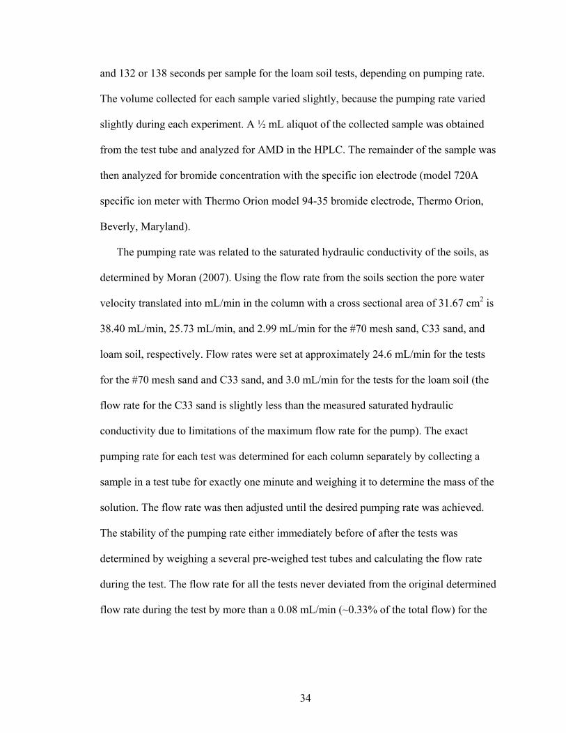
The experimental setup for this test (Figure 3.2) uses an acrylic column (Soil
Measurement Systems, Tucson, AZ) connected to a piston pump (Model QG 50 pump
with QG50-2 pumphead, Fluid Metering Systems, Syosset, NY) with clear vinyl tubing
(Home Depot) that conveys water from the solution flask through the column in an
upward flow direction while a fraction collector (Retriever II model, Teledyne Isco,
Lincoln, Nebraska) collects column effluent in test tubes. The fraction collector was
programmed to collect about 30 samples per pore volume. The fraction collector could
only be programmed to collect samples at six-second increments so the closest setting
was chosen, which was 12 seconds per sample for the #70 mesh sand and C33 sand tests
33
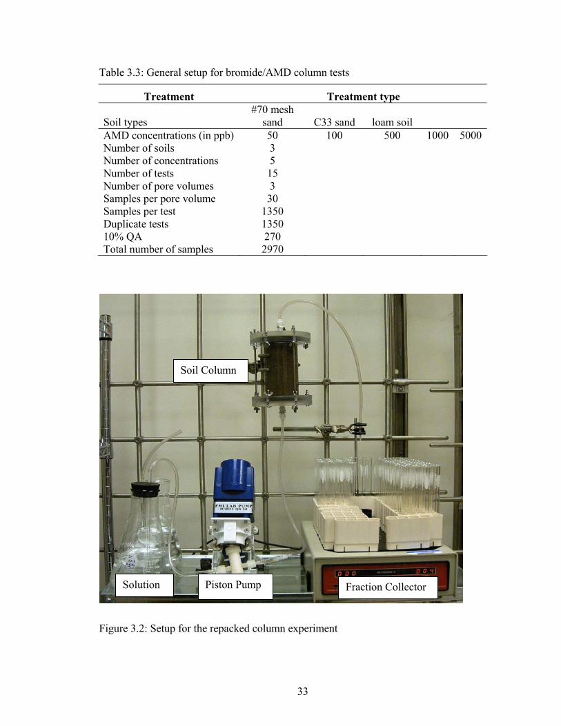
Table 3.3: General setup for bromide/AMD column tests
Treatment Treatment type
Soil types #70 mesh
sand C33 sand
loam soil AMD concentrations (in ppb) 50 100 500 1000 5000 Number of soils 3 Number of concentrations 5 Number of tests 15 Number of pore volumes 3 Samples per pore volume 30 Samples per test 1350 Duplicate tests 1350 10% QA 270 Total number of samples 2970
Figure 3.2: Setup for the repacked column experiment
Piston Pump Fraction Collector
Soil Column
Solution
34
and 132 or 138 seconds per sample for the loam soil tests, depending on pumping rate.
The volume collected for each sample varied slightly, because the pumping rate varied
slightly during each experiment. A ½ mL aliquot of the collected sample was obtained
from the test tube and analyzed for AMD in the HPLC. The remainder of the sample was
then analyzed for bromide concentration with the specific ion electrode (model 720A
specific ion meter with Thermo Orion model 94-35 bromide electrode, Thermo Orion,
Beverly, Maryland).
The pumping rate was related to the saturated hydraulic conductivity of the soils, as
determined by Moran (2007). Using the flow rate from the soils section the pore water
velocity translated into mL/min in the column with a cross sectional area of 31.67 cm2 is
38.40 mL/min, 25.73 mL/min, and 2.99 mL/min for the #70 mesh sand, C33 sand, and
loam soil, respectively. Flow rates were set at approximately 24.6 mL/min for the tests
for the #70 mesh sand and C33 sand, and 3.0 mL/min for the tests for the loam soil (the
flow rate for the C33 sand is slightly less than the measured saturated hydraulic
conductivity due to limitations of the maximum flow rate for the pump). The exact
pumping rate for each test was determined for each column separately by collecting a
sample in a test tube for exactly one minute and weighing it to determine the mass of the
solution. The flow rate was then adjusted until the desired pumping rate was achieved.
The stability of the pumping rate either immediately before of after the tests was
determined by weighing a several pre-weighed test tubes and calculating the flow rate
during the test. The flow rate for all the tests never deviated from the original determined
flow rate during the test by more than a 0.08 mL/min (~0.33% of the total flow) for the
35
#70 mesh sand and C33 sand tests, or by more than 0.03 mL/min (~1.00% of the total
flow) for the loam tests.
In some cases, the sand-packed columns were used a single time, and then were
repacked, and in other cases, the sand-packed columns were used repeatedly. The
columns used for repeated experiments were flushed with at least 5 pore volumes of test
solution similar to Korom (2000) to remove all remaining bromide and AMD before the
next test was started. Laboratory analyses of bromide and AMD confirmed that levels
were below detection limits at the start of subsequent tests.
3.5.2.1 Test solution for column tests
The test solution used for the repacked column experiment was the same used by
Moran (2007). This solution is a 0.005 M CaSO4 (Fisher Scientific) test solution
augmented with 0.3gm/L thymol (J.T. Baker, Phillipsburg, Virginia) as an anti-microbial
agent. This is the standard test solution described by Klute and Dirksen (1986). This
solution was chosen to correlate the experiments from Moran (2007) but also because the
presence of cations is necessary for PAM to flocculate properly. The 0.005 M CaSO4
solution is equivalent to 200 ppm Ca+2 which correlates to the measurements in the canals
in PAM field scale tests (Susfalk et al., 2007). Those results showed that canal samples
contained 71, 196, and 234 ppm of Ca+2. In addition to Ca+2 the canal samples also
contained 22, 89, and 128 ppm of Mg+2, and 38, 189, and 294 ppm of Na+.
To make the test solution for the specific experiments, a concentrated stock solution
of AMD was made by mixing 50 mL of test solution and 250 mg of AMD, creating a
solution of 500 ppm. Then the necessary volume of the stock solution was added to the
volume of the test solution, using the equation:
36
2211 CVCV (9)
where V1 is the volume of the stock solution, C1 is the concentration of the stock solution,
V2 is the volume of the test solution and C2 is the concentration of the test solution.
Sodium bromide (EMD Chemicals) was then added to the test solution at a
concentration of 200 ppm of bromide for all tests, and was pumped simultaneously with
AMD. The concentration of bromide was in accordance with the measurement capacity
of the specific ion electrode which has a minimum detection limit of 1 ppm and a
maximum detection of over 80,000 ppm, though the company recommends at least a two-
order-of-magnitude range for calibration.
3.5.2.2 Soil column preparation
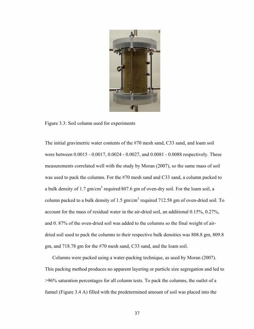
The column used in this experiment is part of a pressure cell apparatus (Figure 3.3)
with dimensions 7.62 cm (3 inch) outside diameter, 6.35 cm (2.5 inches) inside diameter,
15 cm (5.9 inches) in length. The tubing for the column is made of a non reactive acrylic
material.
The C33 sand and loam soil were packed to a target bulk density of 1.7 gm/cm3 and
1.5 gm/cm3, respectively, which are close to known field bulk densities in their natural
undisturbed soil environment. The bulk density chosen for the #70 mesh sand was also
kept at 1.7 gm/cm3.
Initial soil water contents were obtained by weighing 1000 gm of air-dried soil and
then placing it in an oven (Napco model 420, Fisher Scientific) for 105°C for 24 hours to
drive off residual moisture on the soil. The soil was then weighed again and the
gravimetric water content was then calculated as:
g = (mass moist soil – mass oven dry soil)/ (mass oven dry soil)
37
Figure 3.3: Soil column used for experiments
The initial gravimetric water contents of the #70 mesh sand, C33 sand, and loam soil
were between 0.0015 - 0.0017, 0.0024 - 0.0027, and 0.0081 - 0.0088 respectively. These
measurements correlated well with the study by Moran (2007), so the same mass of soil
was used to pack the columns. For the #70 mesh sand and C33 sand, a column packed to
a bulk density of 1.7 gm/cm3 required 807.6 gm of oven-dry soil. For the loam soil, a
column packed to a bulk density of 1.5 gm/cm3 required 712.58 gm of oven-dried soil. To
account for the mass of residual water in the air-dried soil, an additional 0.15%, 0.27%,
and 0. 87% of the oven-dried soil was added to the columns so the final weight of air-
dried soil used to pack the columns to their respective bulk densities was 808.8 gm, 809.8
gm, and 718.78 gm for the #70 mesh sand, C33 sand, and the loam soil.
Columns were packed using a water-packing technique, as used by Moran (2007).
This packing method produces no apparent layering or particle size segregation and led to
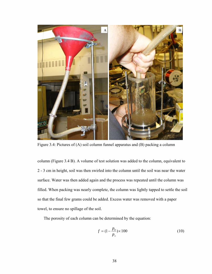
>96% saturation percentages for all column tests. To pack the columns, the outlet of a
funnel (Figure 3.4 A) filled with the predetermined amount of soil was placed into the
38
Figure 3.4: Pictures of (A) soil column funnel apparatus and (B) packing a column
column (Figure 3.4 B). A volume of test solution was added to the column, equivalent to
2 - 3 cm in height, soil was then swirled into the column until the soil was near the water
surface. Water was then added again and the process was repeated until the column was
filled. When packing was nearly complete, the column was lightly tapped to settle the soil
so that the final few grams could be added. Excess water was removed with a paper
towel, to ensure no spillage of the soil.
The porosity of each column can be determined by the equation:
100)1( s
b
p
pf (10)
A B
39
where f is the porosity, pb is the bulk density of the column, and ps is the standard particle
density of a mineral soil, assumed to be 2.65 gm/cm3 (Hillel, 1998). The porosity of the
#70 mesh sand, C33 sand, and the loam soil were determined to be 35.85%, 35.85%, and
43.40% respectively.
The pore volume is the product of the porosity and volume of the soil column, and
was calculated for the #70 mesh sand, C33 sand, and the loam soil to be 170.29 cm3,
170.29 cm3, and 206.15 cm3. The percent saturation for each column is the quotient of the
volumetric water content and pore volume. Pore volumes were determined for each
experiment based on the known mass of soil added to the column assembly, and dividing
by the volume of the column.
3.5.2.3 Pulse and step inputs for breakthrough curves
Two types of boundary conditions are used for the column flow-through experiments:
pulse and step inputs. A pulse experiment is conducted by pumping through a
predetermined amount of test solution (usually in pore volumes) containing a compound
of interest and then pumping through test solution without the chemical of interest to
leach the chemical from the column. Pulse breakthrough curves thus have both an
adsorption and desorption front. If a compound sorbs onto soil and then desorbs during
the leach phase of the experiment, the breakthrough curve exhibits a tailing effect. The
shape adsorption and desorption curves are used to determine the sorption isotherm. A
step experiment is conducted by continuously pumping test solution containing the
compound of interest through the column. A step experiment sometimes uses multiple
(and increasing) concentration steps, which thus yields multiple adsorption fronts
40
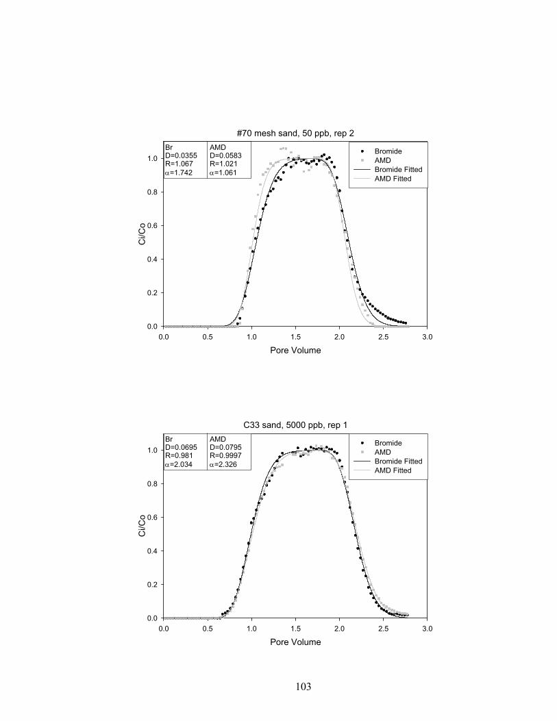
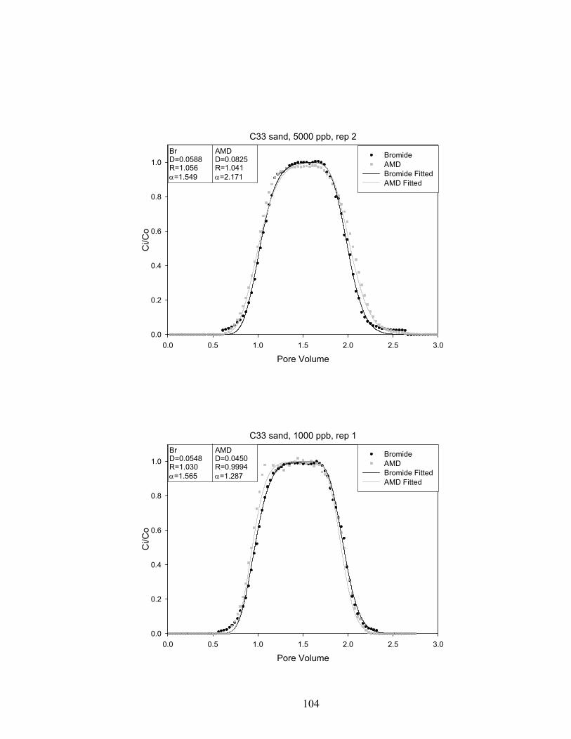
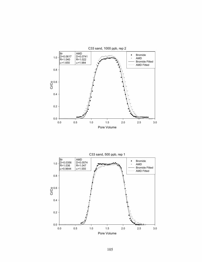
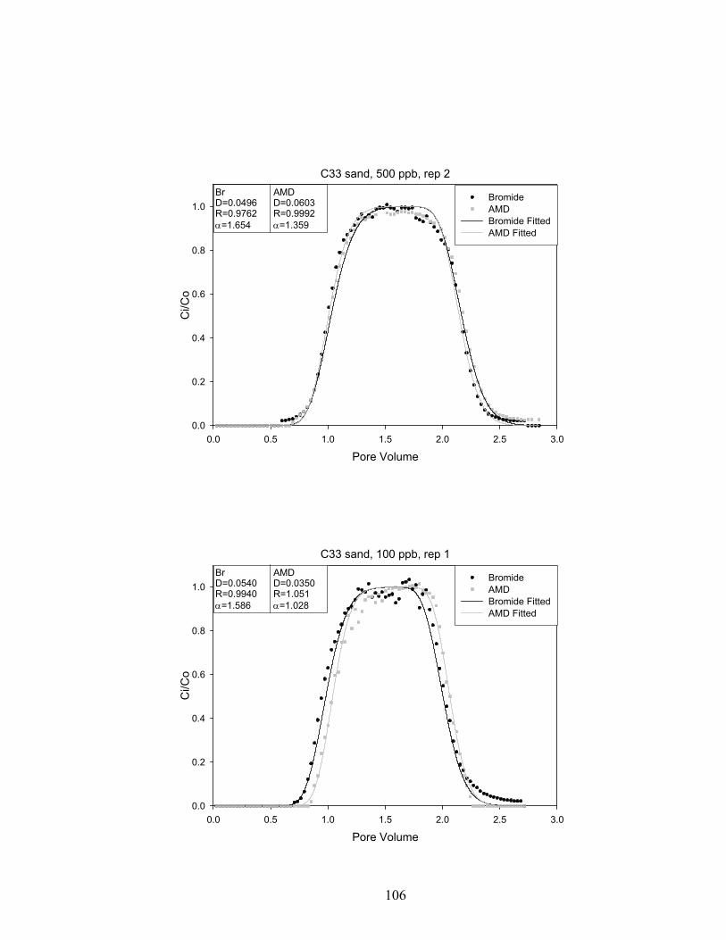
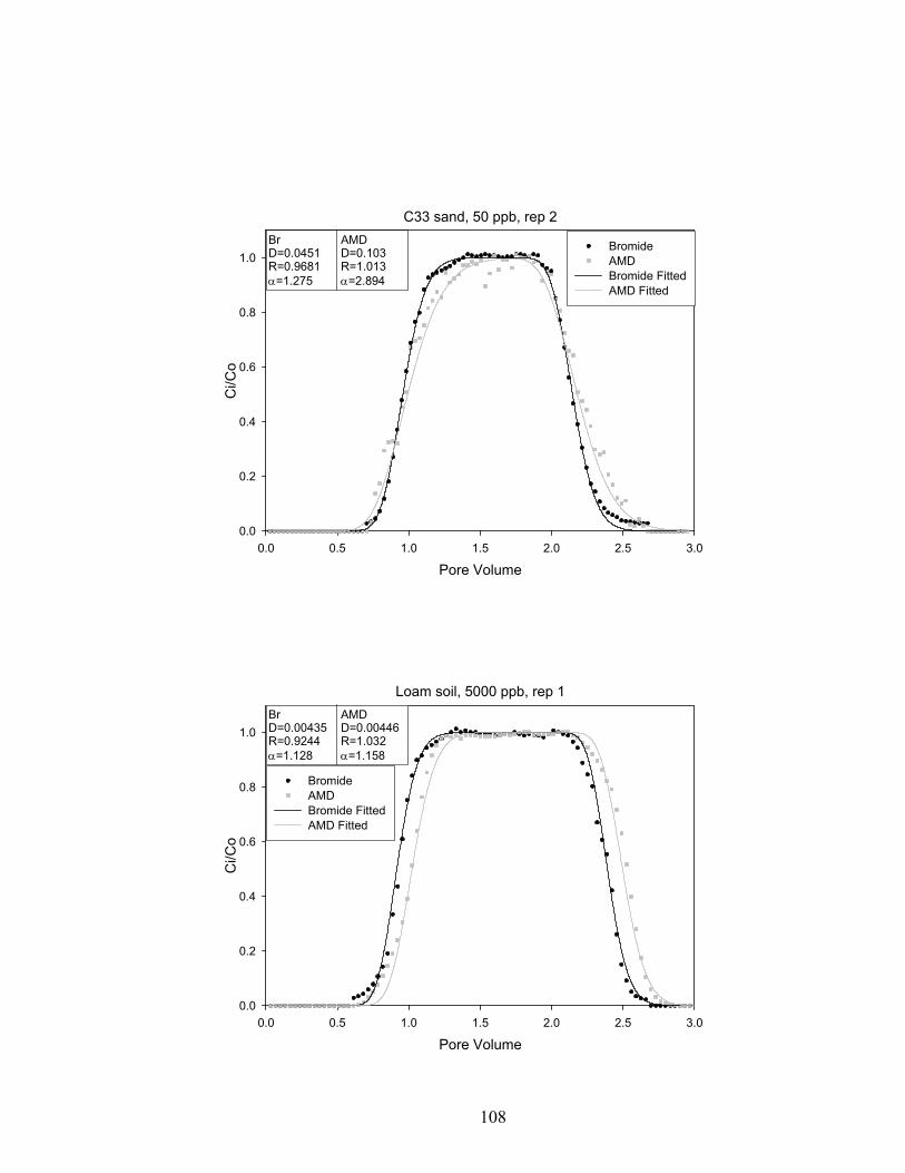
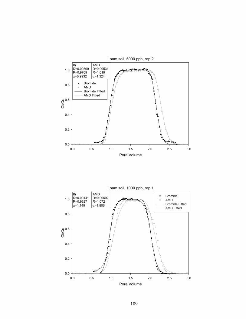
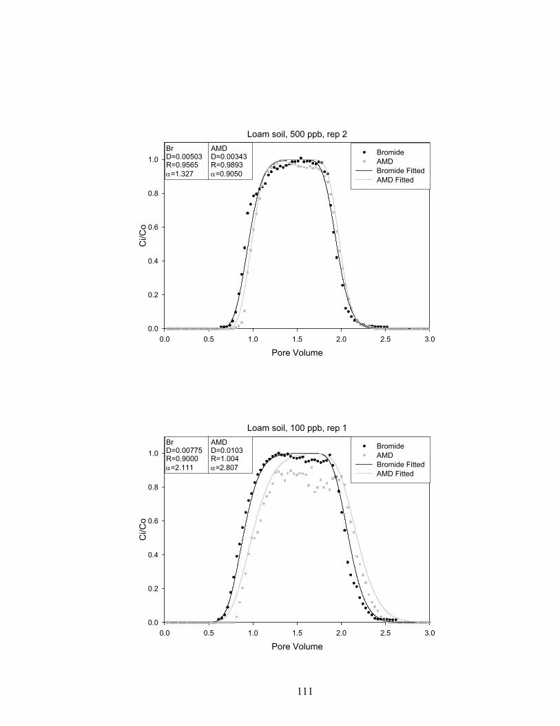
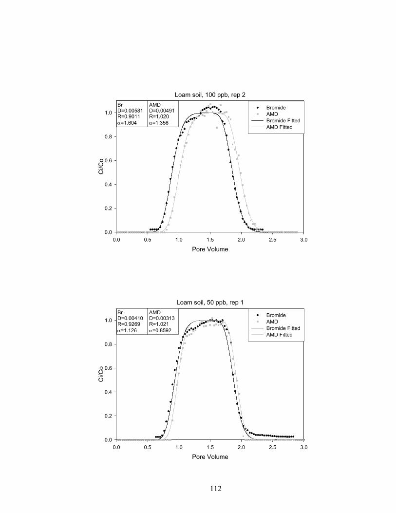
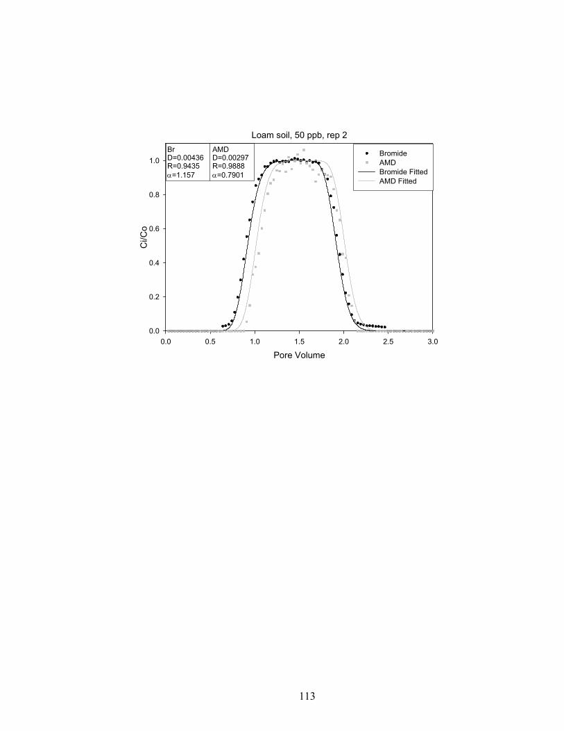
3.5.3 Determining AMD/bromide breakthrough curves
Data from the tests were plotted on graphs of AMD concentration relative to the
initial concentration (Ci/Co) as a function of dimensionless time (i.e., pore volume).
Data were then analyzed using the STANMOD software package (versions 1.0 and 2.0)
(Šimůnek et al., 1999). STANMOD uses a suite of modeling programs (CXTFIT,
CFITM, CFITIM, and CHAIN) that takes experimental effluent data and calculates the
breakthrough curve for a solute based on experimental conditions provide by the user,
and transport parameters, which the program estimates. STANMOD solves the
convective-dispersion equation (CDE) to evaluate solute transport in porous media:
2
2
x
CD
x
Cv
t
C
(11)
where C is concentration, x is the spatial coordinate, v is the average linear velocity, D is
the dispersion coefficient, and t is time. The program estimates solute transport
parameters using a nonlinear least-squares parameter optimization method. By fitting
analytical solutions to the observed column effluent data, the CXTFIT module in
STANMOD predicts retardation factor (R) and dispersion coefficient (D) needed for
predictive modeling using known values of initial concentration, time of sample
collection, pulse application time, pore water velocity (v), and other boundary conditions
to determine the breakthrough curve for a solute.
The pore water velocity for each column was determined by the equation:
Aqv
/ (12)
41
where v is the pore water velocity, q is the flow rate or discharge rate, A is the cross
sectional area of the column, and is the volumetric water content, which is this case is
the porosity.
Concentration for each sample was determined by converting the area response from
the HPLC using the calibration equation obtained as described in section 3.2. Bromide
sample concentration was estimated similarly by converting the millivolt response of the
specific ion electrode using the calibration equation. Samples of the test solution were
collected before the start of each test, and were analyzed for both bromide and AMD
concentration to determine the initial concentration. Each samples concentration was
divided by the initial concentration, yielding the relative concentration (Co/Ci), which
were used for the breakthrough curve analysis. The pore volume at the time of each
sample collection (i.e., used as dimensionless time) was obtained as the product of the
flow rate and the experimental time. The pulse length (in units of time) was multiplied by
the initial concentration to determine the mass of AMD and bromide pumped into the
column for each test. The percent recovery of each tracer was determined as the sum of
the individual masses of tracer collected in each sample (i.e., volume collected in each
sample times the concentration), divided by the total mass of solute added. The Co/Ci and
sample time data were entered into STANMOD and a predicted breakthrough curve was
fitted to the observed data using estimated values of retardation factor (R) and dispersion
coefficient (D). Values of dispersivity (α) were determined using the following equation:
vD / (13)
where v is the pore water velocity.
42
3.5.4 Determining AMD sorption
Methods developed by Burgisser et al. (1993) can then be used to determine the
sorption in the column experiments. To use this method, the hydrodynamic dispersion
coefficient (Ds) must be such that the peclet number is greater than 50, and the sorption
process must be at equilibrium. The peclet number is defined as Pe = Lv / Ds where L is
the length of the column and v is the pore water velocity. A peclet number greater than 50
indicates that the effects of dispersion are minimal and can be ignored (Burgisser et al.,
1993). If these two conditions are met, then the sorption for the column can be
determined by integrating the desorption front using the equation:
sC
pulse
ss dc
t
t
t
ct
pC
0 00
')1)'(
()1(
(14)
where Cs is the sorbed concentration of the chemical of interest, ps is the particle density
of the column, is the porosity of the column, t is the travel time from the first arrival of
the chemical, tpulse is the time duration of the pulse input, t0 is the average travel time
(length of the column divided by the pore water velocity) (Burgisser et al., 1993; Mon et
al., 2006).
3.6 Repacked bacteria inoculated column tests
The C33 sand and loam soil were inoculated with a known AMD-degrading
bacterium and degradation rates were tested using an AMD step concentration of 5 ppm.
Each test was conducted for about 10 pore volumes, at a flow rate of about 1 mL/min in
both soils. Blank tests were also conducted for each soil without inoculated bacteria, to
determine if the sterilization technique used between tests was efficient and effective.
43
Thirty samples per pore volume were taken for the first two pore volumes and fifteen
samples per pore volume for the last eight pore volumes. The extra sampling in the early
stages of the test gave a better resolution for the degree of AMD sorption on the step
breakthrough curve. Sampling for the latter part of the test was reduced to fifteen samples
to limit the waiting time from sample collection to sample analysis in the HPLC.
3.6.1 Experimental setup
The same experimental setup and column packing procedures used in the first set of
column tests was used for this test. Only the C33 sand and loam soil were used for these
experiments. Competing nitrogen sources were added to determine if competing nitrogen
would affect the ability of the bacteria to degrade AMD. Two types of bacteria were used
ones grown in media with 5 ppm AMD added so they would be experienced to degrading
AMD and ones grown in media with no added AMD so they would be naive to seeing
AMD. Additionally, the soils in this set of experiments were autoclaved using the same
method as described in Section 3.3 to ensure that the soil was sterilized of interfering
bacteria. Autoclavable tubing (Pharmed Masterflex silicone tubing, Cole-Parmer, Vernon
Hills, Illinois) was used instead of the clear vinyl tubing and sterilized after each test.
Sterilization of all components of the acrylic soil column and the pump head could not be
done by autoclaving because autoclaving would warp or melt of the acrylic and
negatively affect the ceramic. These pieces were instead soaked in an ethanol solution
and air dried to kill bacteria on the column components and pump apparatus to reduce or
preclude cross-contamination.
44
3.6.1.1 Test solution for column tests
The test solution was changed from that used in the first repacked columns, to ensure
that the bacteria would have a growth medium similar to a natural environment. A
solution of “flow through media” was made to achieve this. Several tests were conducted
in which AMD was the sole nitrogen source, and other tests were conducted in which a
competing source of nitrogen was added to determine whether the competing nitrogen
sources affected the amount of AMD degradation by the bacteria.
Flow through media was a modified form of the M1 medium (Myers and Nealson,
1988) with added calcium to replicate the sodium adsorption ratio (SAR) of the previous
test solutions. The modified test solution, called M1-SAR1 contains 340 mg of CaSO4,
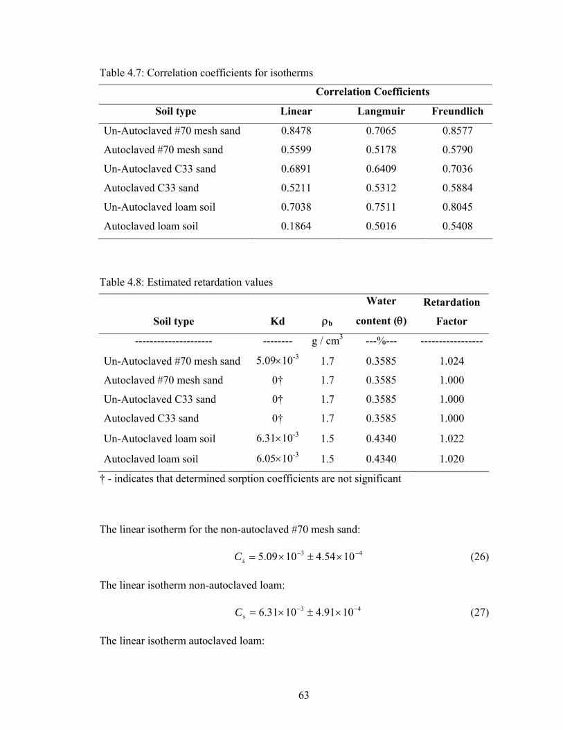
† - indicates that determined sorption coefficients are not significant
The linear isotherm for the non-autoclaved #70 mesh sand:
43 1054.41009.5 sC (26)
The linear isotherm non-autoclaved loam:
43 1091.41031.6 sC (27)
The linear isotherm autoclaved loam:
64
43 1085.81005.6 sC (28)
4.3 Experiment 2: AMD degradation flask study
4.3.1 Flask degradation rates
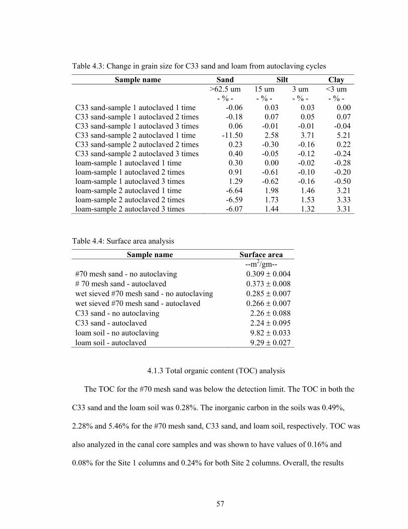
Estimated degradation and AMD half lives for the flask tests are shown in Table 4.9
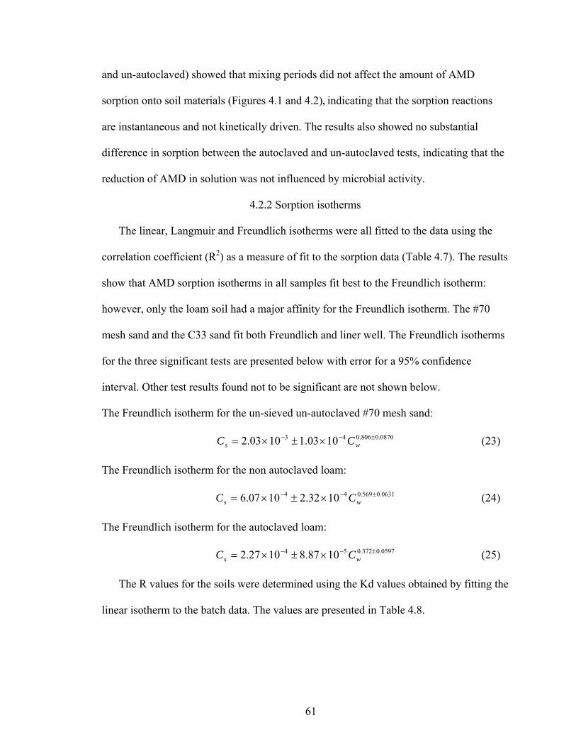
and the graph of the degradation rate fits is shown in Figure 4.3. The test with the fastest
degradation rate was the Closed-Air Open-Light tests. The two samples open to light are
the highest and lowest in degradation indicating that light, at least at the wavelengths
found in the laboratory, had no definitive effect on AMD degradation. Also the samples
closed to air were found to have the two fastest degradation rates. This leads to the
conclusion that having the samples open to air also has no definitive effect on the
degradation of AMD. One possible explanation for the faster AMD degradation in closed
air samples is the potential of contamination from bacteria during sampling. Determining
similarity of degradation rates could not be done because of the lack of replicates and
samples.
The results show a large difference in the degradation rates between the Open-Air
Open-Light test and the Closed-Air Open-Light test. Degradation rates for the other two
treatments were within two standard deviations from the mean of the group of samples.
Results were similar for the half lives as well. The small sample size and large
differences limit the type of statistical analyses that can be performed on the data. The
results indicate that AMD is stable at room temperatures for a long time, thus confirming
that holding times for HPLC analysis (on the order of 12-24 hours) were not an
influencing factor for sample analysis.
65
Table 4.9: Estimated flask degradation values
Test Degradation rate constant
Final degradation Half life
-----hours-1----- --------%-------- ----days---- Open Air Open Light 2.17E-03 26.12 319 Open Air Closed Light 4.06E-03 58.95 171 Closed Air Open Light 1.03E-02 94.79 67 Closed Air Closed Light 6.50E-03 76.09 107
Time (in days)
0 50 100 150 200
N(t
) / N
0
0.0
0.1
0.2
0.3
0.4
0.5
0.6
0.7
0.8
0.9
1.0
1.1
Open air open lightOpen air closed lightClosed air open lightClosed air closed light
Figure 4.3: Graph of flask data and degradation rates (symbols are observed data, lines are fitted degradation rates)
66
4.3.2 Flask sterility analysis
Sampling for bacterial contamination of the flask was first conducted approximately
3.5 months into test. Results showed that the Closed-Air Closed-Light flask contained an
unknown bacterium at and showed an optical density reading of 0.020 OD600. Samples
from the other three flasks registered zero optical density in the spectrophotometer,
indicating that they had not been contaminated. Sampling for a second contamination test
was done approximately 6.5 months (at the end of the test), and the results of these tests
indicated that all four flasks had become contaminated. The Open-Air Open-Light flask,
Open-Air Closed-Light, Closed-Air Open-Light, and Closed-Air Closed-Light flasks
measured 0.032, 0.146, 0.127, and 0.206 OD600 respectively. The higher optical density
readings may indicate a higher bacterial cell count if the cells are of the same type.
Although the cell count can not be derived from this test without calibrating for the
specific type of bacteria, the result at least provides an idea of the level of contamination.
Also, since the bacteria in the flasks were not identified, their potential for AMD
degradation is unknown. Nonetheless, if higher contamination level is indicative of
higher degradation rates, then the optical density test results could partially explain the
substantial difference in the AMD degradation rates in the flasks.
4.4 Experiment 3: repacked column tests
4.4.1 Analysis of breakthrough curves
Table 4.10 presents the percent recovery for AMD and bromide, and the pore water
velocity and water content for each experiment. Tests are identified by soil type,
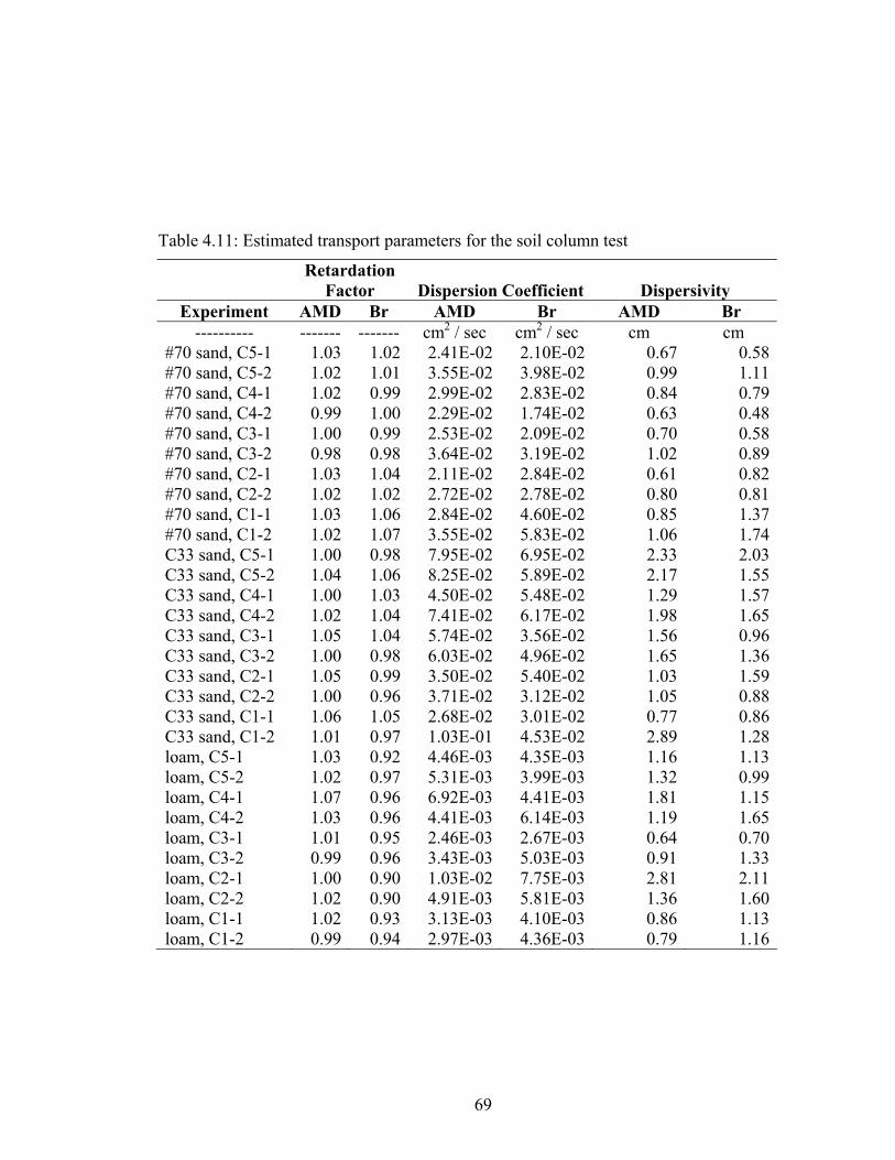
concentration (C5= 5000, C4= 1000, etc.), and experimental replicate. Table 4.11 lists the
67
transport parameters estimated from each of the breakthrough curve experiments
(Appendix I graphs the fitted and modeled data for each experiment). Solute recoveries
tended to be consistently between 95% and 100% for all three soils. Mean recoveries for
#70 mesh sand, C33 sand, and loam soil were 96.17 %, 97.79 %, and 92.27 %
respectively. Values across all three soil types ranged from 81.61% - 105.26%, with the
lowest recovery values in the low concentration loam soils.
Data from the column tests shows that the R values for AMD are close to unity for
every test for every soil type (ranging from 0.98-1.06), indicating that AMD is a
conservative compound. Because the diffusion coefficient for AMD and bromide are so
low, 1.4 10-11 cm2 / s, and 1.0 10-9 cm2 / s respectively (Blaya et al., 2004 and
Maloszewski et al., 1998), the diffusion coefficient was considered to be insignificant.
Values of D and were then used to determine if dispersion in the different soils was
similar.
Using ANOVA, multiple comparison tests, and ANCOVA analyses, R, D, , and
percent recovery were tested for similarity for all initial concentrations and soil types.
The F-values, F-critical values, and P-values for all the ANOVA and ANCOVA analysis
are shown in Table 4.12 and the multiple comparison T-values and P-values are listed in
Table 4.13. Test results show that R for AMD is similar for all soil types and
concentrations. The D values, however, were determined to be statistically different.
Multiple comparison tests were done to determine which soil led to differences in D. The
results showed that #70 mesh sand, C33 sand, and the loam soil were all significantly
different from each other, indicating that the different grain size distributions in the soils
are causing differences in the flow characteristics in the columns. Initial concentrations
68
Table 4.10: Recovery and experimental conditions for soil column experiments
of AMD had no affect the dispersion coefficient. The values in all soils were
determined to be statistically different. Multiple comparisons showed that the #70 mesh
sand and the C33 sand were significantly different, but the C33 sand versus loam soil and
the #70 mesh sand versus loam tests proved to be similar; however, the P value for both
these comparisons was very low, indicating a statistically significant effect of only
when comparing results from the #70 mesh and the C33 sands. The in all initial
concentrations of AMD was determined to be similar. The percent recoveries for AMD in
all soils were determined to be statistically different. Multiple comparison tests showed
different recoveries between the C33 sand and the loam soil, while the other comparisons
were similar. These results indicate a lower than expected recovery for the loam soil
compared to recoveries in the C33 sand (recovery in the #70 mesh sand was similar to the
loam soil). Low recovery in the loam could be due to several factors, including possible
bacterial contamination of the loam soil, causing a small amount of degradation, a small
amount of chemical breakdown in the AMD due to the presence of charged clay particles
in the loam soil or possible error in the determination of the AMD peak in the HPLC due
to fine clays interfering with the integration. Initial concentration had no effect on the
percent recoveries, although the low P value for this test shows a possible trend.
4.4.2 Column sorption isotherms
All column peclet numbers were determined to be greater than 300, which is much
greater than the 50 needed, which confirms that the methods in Section 3.5.4 can be used
to analyze the column tests for sorption. The individual values of sorption for each
concentration level were then plotted in Tablecurve and fitted to different forms of
sorption isotherms to determine which form fit the data most closely.
71
Table 4.12: ANOVA and ANCOVA statistics for AMD parameter comparisons
Test F-value F-Critical
value P-value Effect ANOVA - AMD R vs. soil type 0.389 3.710 0.681 NOANOVA - AMD R vs. initial concentration 0.331 3.330 0.570 NOANCOVA - AMD R vs. soil type vs. concentration 0.358 NA† 0.784 NOANOVA - AMD D vs. soil type 36.184 3.710 0.0001 YESANOVA - AMD D vs. initial concentration 0.246 3.330 0.909 NOANOVA - vs. soil type 6.277 3.710 0.006 YESANOVA - vs. concentration 0.231 3.330 0.918 NOANOVA - AMD percent recoveries vs. soil type 4.506 3.710 0.020 YESANOVA - AMD percent recoveries vs. concentration 1.822 3.330 0.156 NO
†NA- ANCOVA tests do not have F-critical values
Table 4.13: Multiple comparison statistics for parameter comparisons
Test T-value T-test
P-value Effect MC test- AMD D in #70 mesh sand vs. C33 sand 8.408 0.0001 YESMC test- AMD D in #70 mesh sand vs. loam soil 4.824 0.0001 YESMC test- AMD D C33 sand vs. loam soil 3.656 0.0003 YESMC test- AMD in #70 mesh sand vs. C33 sand 3.538 0.004 YESMC test- AMD in #70 mesh sand vs. loam soil 1.934 0.261 NOMC test- AMD C33 sand vs. loam soil 1.604 0.149 NOMC test- AMD percent recovery in #70 mesh sand vs. C33 sand 0.856 0.6720 NOMC test- AMD percent recovery in #70 mesh sand vs. loam soil 2.064 0.1160 NOMC test- AMD percent recovery C33 sand vs. loam soil 2.920 0.0190 YES
72
Similar to results found for the batch experiments, the linear and Freundlich isotherms
provided good fits to the data (Table 4.14). The Freundlich isotherms for the tests are
presented below with error for a 95% confidence interval.
The Freundlich isotherm for the #70 mesh sand:
0042.0009.132 1030.11024.5 ws CC (29)
The Freundlich isotherm for the C33 sand:
0157.0026.132 1062.51000.6 ws CC (30)
The Freundlich isotherm for the loam soil:
0274.0109.132 1026.21035.1 ws CC (31)
4.4.2 Comparing batch and column sorption isotherms and retardation values
Parameters in the sorption isotherms calculated in the batch studies are less than those
calculated in the column tests for all soils; however, when the three significant sorption
isotherms from the batch studies were compared to the three isotherms from the column
studies using ANOVA statistical analysis, they were determined to be statistically similar
(F < F critical = 0.414 < 9.55 P = 0.636) for batch isotherms versus column isotherms.
This test was conducted on only 3 samples for each set and this may induce error into the
test, but given that there are no experimental outliers in the transport parameters that were
identified from the data, the three randomly-sampled values used in the comparison
should be valid.
The mean values for R for the batch studies were compared to those obtained from
the column tests. The R values were 1.024, 1.000, and 1.022 for batch studies and 1.014,
1.023, and 1.018 for the column tests, using for the #70 mesh sand, C33 soil and the loam
soil respectively. This shows good correlation between the two experimental methods.
73
Table 4.14: Correlation coefficients for isotherms
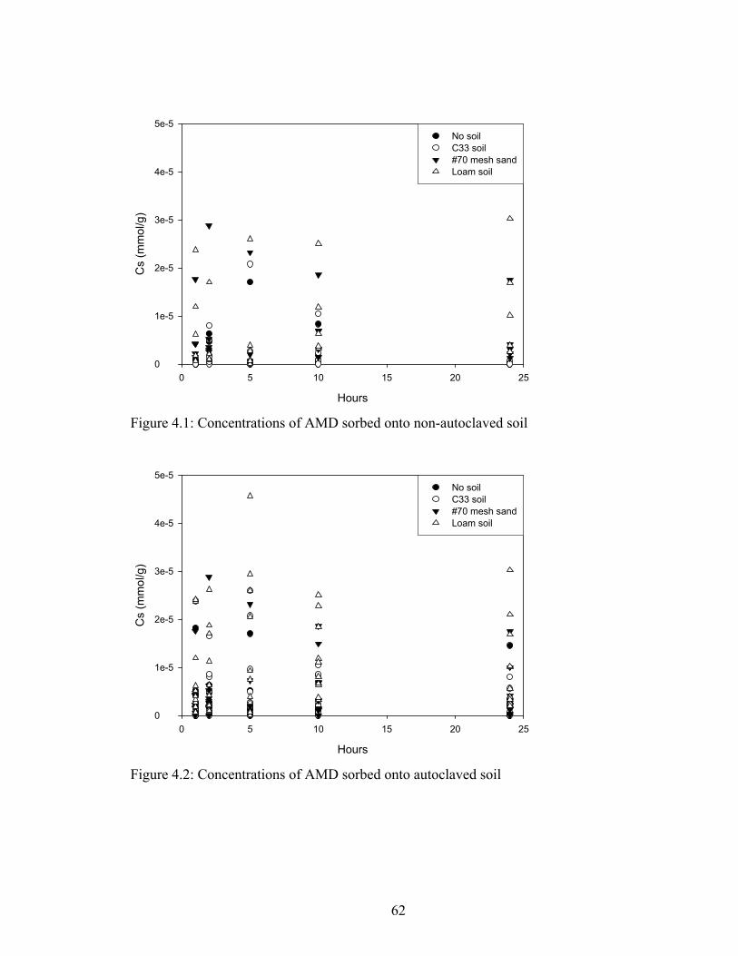
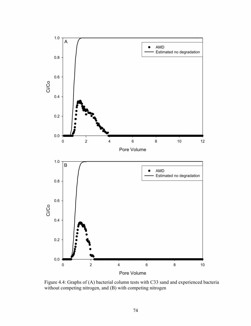
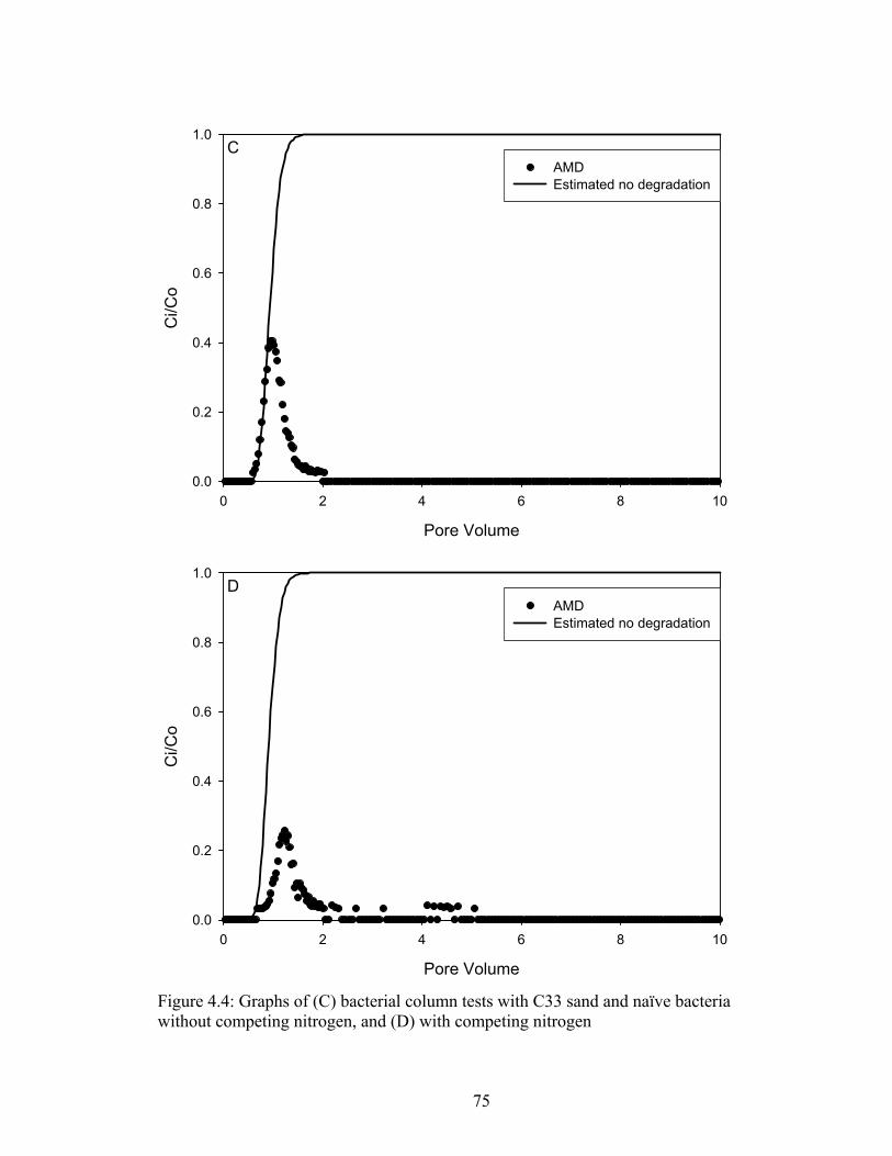
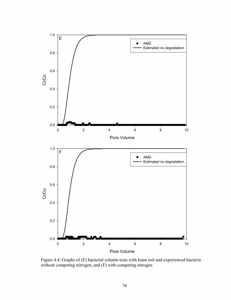
Data used in the breakthrough curve analysis were obtained using the same methods
as described in section 4.3.1. Specifically, the experiments yielded AMD concentration
with time. Using column parameters as described earlier (i.e., pore water velocity, initial
concentration, etc.) for each experiment, STANMOD was used to predict the
breakthrough curve, assuming no degradation. Experiments were varied by soil, absence
or presence of competing nitrogen and type of bacteria. These graphs are shown in
Figures 4.4 A-J. The experiments are labeled by soil type, competing nitrogen (N+ for
competing nitrogen added, N- for no competing nitrogen), and the type of bacteria (e for
experienced, n for naïve, and x for no bacteria).
4.5.2 Bacteria column degradation rates and half lives
Estimated degradation rates and half-lives for the column tests are shown in Table
4.15. The final degradation percentage is calculated as ([1 – Co/Ci]*100%), which is a
measure of the concentration of AMD in the final sample taken for each test. This
parameter is essentially a gauge for the effectiveness of the bacteria at degrading AMD
after a three-hour contact period in the column. Note that the degradation rates are much
74
Pore Volume
0 2 4 6 8 10 12
Ci/C
o
0.0
0.2
0.4
0.6
0.8
1.0
AMDEstimated no degradation
A
Pore Volume
0 2 4 6 8 10
Ci/C
o
0.0
0.2
0.4
0.6
0.8
1.0
AMDEstimated no degradation
B
Figure 4.4: Graphs of (A) bacterial column tests with C33 sand and experienced bacteria without competing nitrogen, and (B) with competing nitrogen
75
Pore Volume
0 2 4 6 8 10
Ci/C
o
0.0
0.2
0.4
0.6
0.8
1.0
AMDEstimated no degradation
C
Pore Volume
0 2 4 6 8 10
Ci/C
o
0.0
0.2
0.4
0.6
0.8
1.0
AMDEstimated no degradation
D
Figure 4.4: Graphs of (C) bacterial column tests with C33 sand and naïve bacteria without competing nitrogen, and (D) with competing nitrogen
76
Pore Volume
0 2 4 6 8 10
Ci/C
o
0.0
0.2
0.4
0.6
0.8
1.0
AMDEstimated no degradation
E
Pore Volume
0 2 4 6 8 10
Ci/C
o
0.0
0.2
0.4
0.6
0.8
1.0
AMDEstimated no degradation
F
Figure 4.4: Graphs of (E) bacterial column tests with loam soil and experienced bacteria without competing nitrogen, and (F) with competing nitrogen
77
Pore Volume
0 2 4 6 8 10
Ci/C
o
0.0
0.2
0.4
0.6
0.8
1.0
AMDEstimated no degradation
G
Pore Volume
0 2 4 6 8 10
Ci/C
o
0.0
0.2
0.4
0.6
0.8
1.0
AMDEstimated no degradation
H
Figure 4.4: Graphs of (G) bacterial column tests with loam soil and experienced bacteria without competing nitrogen, and (H) with competing nitrogen
78
Pore Volume
0 2 4 6 8 10
Ci/C
o
0.0
0.2
0.4
0.6
0.8
1.0
AMDEstimated no degradation
I
Pore Volume
0 2 4 6 8 10
Ci/C
o
0.0
0.2
0.4
0.6
0.8
1.0
AMDEstimated no degradation
J
Figure 4.4: Graphs of (I) bacterial column tests with C33 sand, no bacteria, without competing nitrogen, and (J) loam soil, no bacteria, without competing nitrogen
79
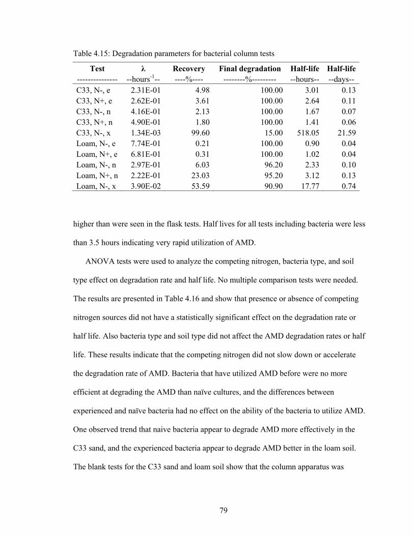
Table 4.15: Degradation parameters for bacterial column tests
Test λ Recovery Final degradation Half-life Half-life--------------- --hours-1-- ----%---- --------%--------- --hours-- --days-- C33, N-, e 2.31E-01 4.98 100.00 3.01 0.13C33, N+, e 2.62E-01 3.61 100.00 2.64 0.11C33, N-, n 4.16E-01 2.13 100.00 1.67 0.07C33, N+, n 4.90E-01 1.80 100.00 1.41 0.06C33, N-, x 1.34E-03 99.60 15.00 518.05 21.59Loam, N-, e 7.74E-01 0.21 100.00 0.90 0.04Loam, N+, e 6.81E-01 0.31 100.00 1.02 0.04Loam, N-, n 2.97E-01 6.03 96.20 2.33 0.10Loam, N+, n 2.22E-01 23.03 95.20 3.12 0.13Loam, N-, x 3.90E-02 53.59 90.90 17.77 0.74
higher than were seen in the flask tests. Half lives for all tests including bacteria were less
than 3.5 hours indicating very rapid utilization of AMD.
ANOVA tests were used to analyze the competing nitrogen, bacteria type, and soil
type effect on degradation rate and half life. No multiple comparison tests were needed.
The results are presented in Table 4.16 and show that presence or absence of competing
nitrogen sources did not have a statistically significant effect on the degradation rate or
half life. Also bacteria type and soil type did not affect the AMD degradation rates or half
life. These results indicate that the competing nitrogen did not slow down or accelerate
the degradation rate of AMD. Bacteria that have utilized AMD before were no more
efficient at degrading the AMD than naïve cultures, and the differences between
experienced and naïve bacteria had no effect on the ability of the bacteria to utilize AMD.
One observed trend that naive bacteria appear to degrade AMD more effectively in the
C33 sand, and the experienced bacteria appear to degrade AMD better in the loam soil.
The blank tests for the C33 sand and loam soil show that the column apparatus was
80
Table 4.16: Results of ANOVA analyses for parameter comparisons
Test F-value F-Critical
value P-value Effect Competing nitrogen vs. degradation rate 0.009 6.940 0.926 NOCompeting nitrogen vs. half life 0.012 6.940 0.916 NOBacterial type vs. degradation rate 0.730 6.940 0.729 NOBacterial type vs. half life 0.132 6.940 0.426 NOSoil type vs. degradation rate 0.911 6.940 0.377 NOSoil type vs. half life 0.268 6.940 0.623 NO
properly sterilized between tests, as seen by the close match between experimental and
estimated concentrations.
4.5.3 Bacterial and competing nitrogen analysis
Bacterium used in the column tests was determined by 16S RNA gene sequencing
(Nevada Genomics Center, Reno, Nevada) to be Pseudomonas putida (gene sequencing
work was done by Labahn (2007) as part of the collaborative PAM study). These tests
also show that the concentration of bacterial cells in the bacteria column tests were about
1012 cells per gram of soil, a much higher concentration than was analyzed from samples
collected at other field sites (not related to this thesis). The bacteria in these tests were
grown with nutrient media and inoculated for 24 hours, allowing them to thrive in the
column.
Labahn (2007) analyzed the total ammonia and nitrogen for the column tests
conducted with competing nitrogen sources. These samples were taken during the
experiments at 2.5, 5, 7.5 and 10 pore volumes. Labahn (2007) showed that bacteria were
able to fully utilize the nitrogen added to the column through the growth media, and that
the ammonia added to the column through the growth media and the ammonia created
81
from AMD degradation were both partially utilized. The total ammonia concentration
never exceed 1 ppm, which indicates that the added ammonia was degraded at a rate
faster than ammonia was created by AMD degradation. The ammonia from both sources
(added and produced from AMD degradation) however, could not be discriminated.
4.6 Experiment 5: canal soil core column tests
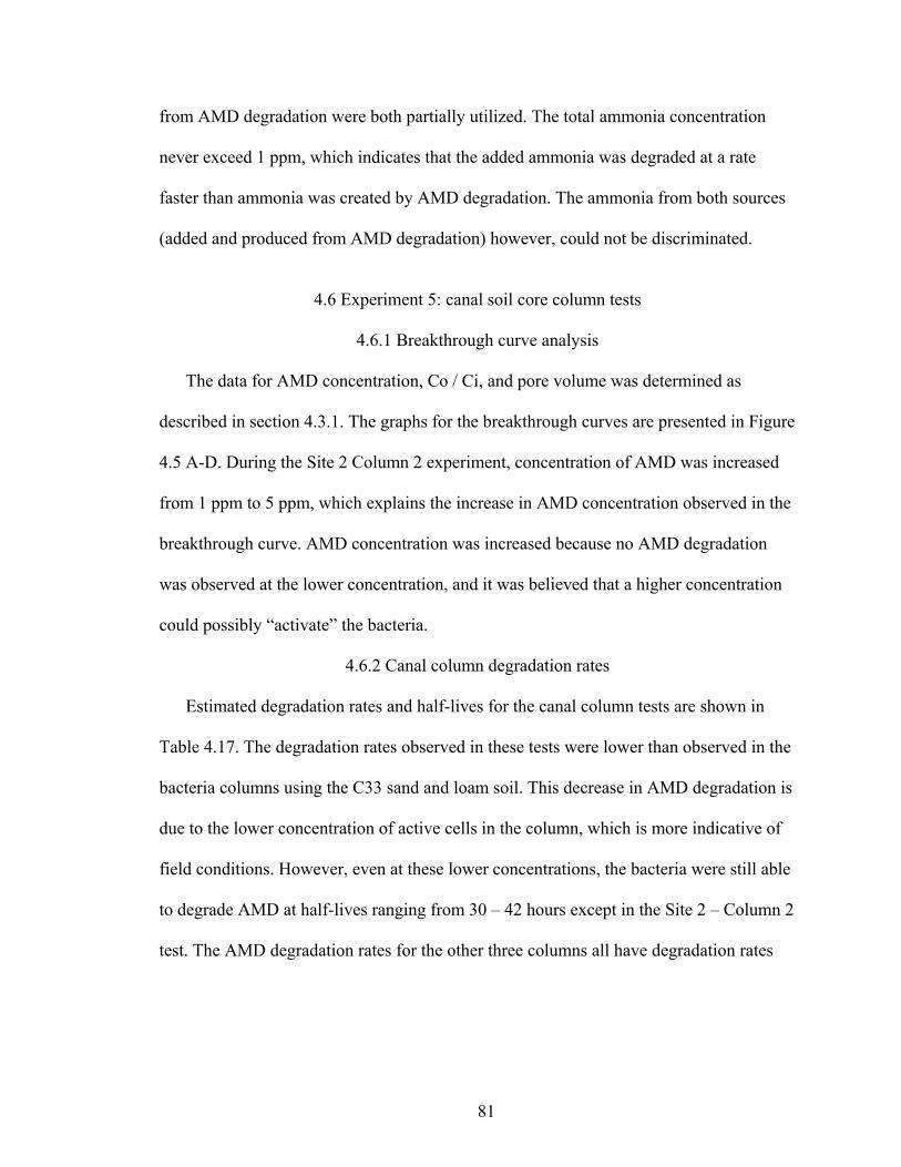
4.6.1 Breakthrough curve analysis
The data for AMD concentration, Co / Ci, and pore volume was determined as
described in section 4.3.1. The graphs for the breakthrough curves are presented in Figure
4.5 A-D. During the Site 2 Column 2 experiment, concentration of AMD was increased
from 1 ppm to 5 ppm, which explains the increase in AMD concentration observed in the
breakthrough curve. AMD concentration was increased because no AMD degradation
was observed at the lower concentration, and it was believed that a higher concentration
could possibly “activate” the bacteria.
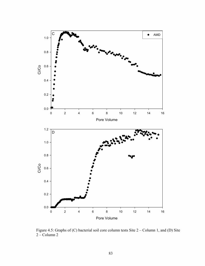
4.6.2 Canal column degradation rates
Estimated degradation rates and half-lives for the canal column tests are shown in
Table 4.17. The degradation rates observed in these tests were lower than observed in the
bacteria columns using the C33 sand and loam soil. This decrease in AMD degradation is
due to the lower concentration of active cells in the column, which is more indicative of
field conditions. However, even at these lower concentrations, the bacteria were still able
to degrade AMD at half-lives ranging from 30 – 42 hours except in the Site 2 – Column 2
test. The AMD degradation rates for the other three columns all have degradation rates
82
Pore Volume
0 2 4 6 8 10
Ci/C
o
0.0
0.2
0.4
0.6
0.8
1.0AMDA
Pore Volume
0 2 4 6 8 10
Ci/C
o
0.0
0.2
0.4
0.6
0.8
1.0AMDB
Figure 4.5: Graphs of (A) bacterial soil core column tests Site 1 – Column 1, and (B) Site 1 – Column 2
83
Pore Volume
0 2 4 6 8 10 12 14 16
Ci/C
o
0.0
0.2
0.4
0.6
0.8
1.0AMDC
Pore Volume
0 2 4 6 8 10 12 14 16
Ci/C
o
0.0
0.2
0.4
0.6
0.8
1.0
1.2D
Figure 4.5: Graphs of (C) bacterial soil core column tests Site 2 – Column 1, and (D) Site 2 – Column 2
84
Table 4.17: Degradation parameters for bacterial column tests
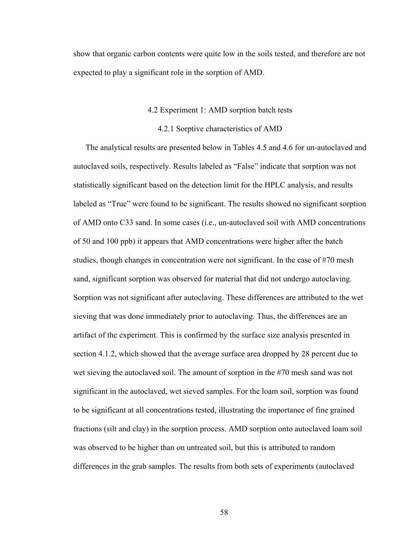
Figure 4.6: Graphs of a HYDRUS model run (C33 sand, partial seal, PAM conductivity level of 10 lb/ca, at water table depth of 0 meters) (A) with out sorption or bacterial degradation and, (B) with the added affects of sorption and bacterial degradation
90
The results showed that the different water table heights change the average flow
length of the solute plume. For example, solute plumes traveled 27.08, 29.37, and 32.01
meters for water table depths of 2, 5, and 10 m, respectively. The saturated hydraulic
conductivities for the different soil types lead to differences in the arrival times and
maximum concentration levels. The earliest arrival times and the peak concentrations
corresponded to the #70 mesh and C33 sands, materials with the highest hydraulic
conductivities.
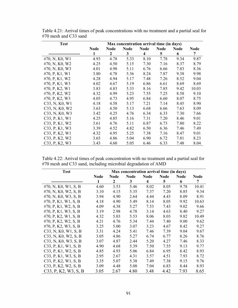
The average arrival times for simulations using the loam soil, with full and partial
seals, ranged from 47 - >50 days at Node 5. The average arrival time for simulations
using the sandy soils, with partial seals ranged from 28 - > 50 days for shallow water
tables, with slightly longer arrival times at Node 5 for the W3 experiments (water table at
10 m depth). The arrival at Node 6 for these experiments was greater than 50 days. The
arrival time of the no and partial seal sand tests for the no sorption and bacterial
degradation tests are provided in Tables 4.21 and 4.22. These results show the sensitivity
of contaminant plume travel time to the degree of seal from PAM treatment. Also the
arrival time of the peak concentration changed slightly when bacterial degradation was
accounted for, because of the effects of degradation on the peak concentration. The
arrival times at Node 7 range from 7.5 to 10.5 days as shown in Tables 4.21 and 4.22.
The flushing effect of uncontaminated water after the 5-day pulse, and the mixing with
the uncontaminated ground water caused a 20-30% reduction in peak concentration at
Node 7 (Table 4.18), for the cases with no PAM treatment (i.e., no seal). The full seal
reduced the amount of flow into the soil system by 90% (Table 4.18). This simulation
result correlates with the reduction in seepage seen in Moran (2007). The decreased
91
Table 4.21: Arrival times of peak concentrations with no treatment and a partial seal for #70 mesh and C33 sand
Characterization: Using Linear Anionic Polyacrylamide (LA-PAM) to Reduce
122
Water Seepage from Unlined Water Delivery Canal Systems. DRI Publication
No. 41226.
123
VITA
Graduate College University of Nevada, Las Vegas
Todd J. Arrowood
Home Address: 8044 Secretariat lane Las Vegas, NV 89123
Degrees:
Bachelor of Science, Geoscience, 2005 University of Nevada, Las Vegas
Publications: Arrowood, T., and Young, M.H. 2007. AMD sorption in soil/water systems in, Results of
Laboratory Experiments in Support of PAM-Related Research, M.H. Young, Editor. DRI Publication No. 41237.
Presentations: Arrowood, T., Young, M.H., 2007, Determining the Transport of the Acrylamide
Monomer (AMD) in Soil and Groundwater Systems, UNLV Geosymposium Arrowood, T., Young, M.H., Yu, Z. 2006, Determining the Transport of the Acrylamide
Monomer (AMD) in Soil and Groundwater Systems, UNLV Geosymposium Arrowood, T., Young, M.H., Yu, Z., Lahban, S., and Moser, D. 2007, Fate and Transport
of Acrylamide in soil and groundwater systems: Sorption, Retardation and Numerical Simulations, Presented at the American Geophysical Union, Fall Meetings, San Francisco, CA
Lahban, S., Moser, D., Arrowood, T., Young, M.H., and Robleto, E. 2007, Fate of Acrylamide in Soil and Groundwater Systems: Microbial Degradation, Presented at the American Geophysical Union, Fall Meetings, San Francisco, CA
Thesis Title: Determining the Fate and Transport of the Acrylamide Monomer (AMD) in Soil and Groundwater Systems.
Thesis Examination Committee:
Chairperson, Dr. Zhongbo Yu, Ph.D. Co-Chairperson, Dr. Michael Young, Ph.D. Committee Member, Dr. Dave Kreamer, Ph.D. Graduate Faculty Representative, Dr. Thomas Piechota, Ph.D.