Deterministic signal associated with a random field

Deterministic signal associated with a random field

Taewoo Kim,1 Ruoyu Zhu,1 Tan H. Nguyen,1 Renjie Zhou,2 Chris Edwards,2 Lynford L. Goddard,2 and Gabriel Popescu1,*

1Quantitative Light Imaging Laboratory, Department of Electrical and Computer Engineering, Beckman Institute for Advanced Science and Technology, University of Illinois at Urbana-Champaign, Urbana, Illinois 61801, USA

2Photonic Systems Laboratory, Department of Electrical and Computer Engineering, Micro and Nanotechnology Laboratory, University of Illinois at Urbana-Champaign, Urbana, Illinois 61801, USA

*[email protected]

Abstract: Stochastic fields do not generally possess a Fourier transform. This makes the second-order statistics calculation very difficult, as it requires solving a fourth-order stochastic wave equation. This problem was alleviated by Wolf who introduced the coherent mode decomposition and, as a result, space-frequency statistics propagation of wide-sense stationary fields. In this paper we show that if, in addition to wide-sense stationarity, the fields are also wide-sense statistically homogeneous, then monochromatic plane waves can be used as an eigenfunction basis for the cross spectral density. Furthermore, the eigenvalue associated with a plane wave, exp[ ( )]i tω⋅ −k r , is given by the spatiotemporal power spectrum

evaluated at the frequency (k, ω). We show that the second-order statistics of these fields is fully described by the spatiotemporal power spectrum, a real, positive function. Thus, the second-order statistics can be efficiently propagated in the wavevector-frequency representation using a new framework of deterministic signals associated with random fields. Analogous to the complex analytic signal representation of a field, the deterministic signal is a mathematical construct meant to simplify calculations. Specifically, the deterministic signal associated with a random field is defined such that it has the identical autocorrelation as the actual random field. Calculations for propagating spatial and temporal correlations are simplified greatly because one only needs to solve a deterministic wave equation of second order. We illustrate the power of the wavevector-frequency representation with calculations of spatial coherence in the far zone of an incoherent source, as well as coherence effects induced by biological tissues.

©2013 Optical Society of America

OCIS codes: (030.1640) Coherence; (030.1670) Coherent optical effects; (030.6600) Statistical optics; (170.3660) Light propagation in tissues; (290.5825) Scattering theory.

Reference and links

1. L. Mandel and E. Wolf, Optical Coherence and Quantum Optics (Cambridge University Press, 1995), pp. xxvi, 1166 p.

2. J. W. Goodman, Statistical Optics, Wiley classics library ed., Wiley classics library (Wiley, 2000), pp. xvii, 550 p.

3. G. Popescu, Quantitative Phase Imaging of Cells and Tissues, McGraw-Hill biophotonics (McGraw-Hill, 2011), p. 385.

4. Z. Wang and G. Popescu, “Quantitative phase imaging with broadband fields,” Appl. Phys. Lett. 96(5), 051117 (2010).

5. R. J. Glauber, “The quantum theory of optical coherence,” Phys. Rev. 130(6), 2529–2539 (1963). 6. M. Born and E. Wolf, Principles of Optics: Electromagnetic Theory of Propagation, Interference and

Diffraction of Light, 7th expanded ed. (Cambridge University Press, 1999).

#189465 - $15.00 USD Received 25 Apr 2013; revised 31 Jul 2013; accepted 1 Aug 2013; published 29 Aug 2013(C) 2013 OSA 9 September 2013 | Vol. 21, No. 18 | DOI:10.1364/OE.21.020806 | OPTICS EXPRESS 20806

7. E. Wolf, Introduction to the Theory of Coherence and Polarization of Light (Cambridge University Press, 2007), pp. xiv, 222 p.

8. E. Wolf, “New spectral representation of random sources and of the partially coherent fields that they generate,” Opt. Commun. 38(1), 3–6 (1981).

9. E. Wolf, “New theory of partial coherence in the space-frequency domain. 1. Spectra and cross spectra of steady-state sources,” J. Opt. Soc. Am. 72(3), 343–351 (1982).

10. E. Wolf, “New theory of partial coherence in the space-frequency domain. 2. Steady-state fields and higher-order correlations,” J. Opt. Soc. Am. A 3, 76–85 (1986).

11. D. Huang, E. A. Swanson, C. P. Lin, J. S. Schuman, W. G. Stinson, W. Chang, M. R. Hee, T. Flotte, K. Gregory, C. A. Puliafito, and J. G. Fujimoto, “Optical coherence tomography,” Science 254(5035), 1178–1181 (1991).

12. T. S. Ralston, D. L. Marks, P. S. Carney, and S. A. Boppart, “Interferometric synthetic aperture microscopy,” Nat. Phys. 3(2), 129–134 (2007).

13. C. A. Puliafito, M. R. Hee, J. S. Schuman, and J. G. Fujimoto, Optical Coherence Tomography of Ocular Diseases (Slack, Inc., 1995).

14. D. Lim, K. K. Chu, and J. Mertz, “Wide-field fluorescence sectioning with hybrid speckle and uniform-illumination microscopy,” Opt. Lett. 33(16), 1819–1821 (2008).

15. Z. Wang, L. J. Millet, M. Mir, H. Ding, S. Unarunotai, J. A. Rogers, M. U. Gillette, and G. Popescu, “Spatial light interference microscopy (SLIM),” Opt. Express 19(2), 1016–1026 (2011).

16. R. Zhu, S. Sridharan, K. Tangella, A. Balla, and G. Popescu, “Correlation-induced spectral changes in tissues,” Opt. Lett. 36(21), 4209–4211 (2011).

17. J. Shamir, “Optical Systems and Processes, Vol,” PM65 of the SPIE Press Monographs (SPIE, 1999). 18. P. Langevin, “On the theory of Brownian motion,” C. R. Acad. Sci. (Paris) 146, 530 (1908).

1. Introduction

Random field fluctuations in both space and time are due to the respective fluctuations of both primary and secondary sources. The discipline that studies these fluctuations is known as coherence theory or statistical optics [1, 2]. Besides its importance to basic science, coherence theory is crucial in predicting outcomes of many light experiments. For example, in quantitative phase imaging (QPI), we often employ spatially and temporally broadband light to image phase shifts associated with the imaging field [3]. Such phase shifts are physically meaningful only when they are defined via averages, through field cross-correlations (see, e.g., [4]). Whenever we measure a superposition of fields (e.g., in interferometry) the result of the statistical average performed by the detection process is strongly dependent on the coherence properties of the light. Importantly, half of the 2005 Nobel Prize in Physics was awarded to Roy Glauber “for his contribution to the quantum theory of optical coherence.” For a selection of Glauber’s seminal papers, see Ref [5].

A thermal source, such as an incandescent filament or the surface of the Sun, emits light in a manner that cannot be predicted with certainty. In other words, unlike in the case of a monochromatic plane wave, we cannot find a function f(r,t) that prescribes the field at each point in space and at each moment in time. Instead, we describe the source as emitting a random signal, s(r,t), and describe its behavior via probability distributions.

We can gain knowledge about the random process only by repetitive measurements and averaging the results. This type of averaging over many realizations of a certain random variable is called ensemble averaging. The importance of the ensemble averaging has been emphasized many times by both Wolf and Glauber [1, 5–7]. For example, on page 29 of Ref [5], Glauber mentions “It is important to remember that this average is an ensemble average. To measure it, we must in principle repeat the experiment many times by using the same procedure for preparing the field over and over again. That may not be a very convenient procedure to carry out experimentally but it is the only one which represents the precise meaning of our calculation.”

Calculating how field correlations behave upon propagation requires solving a stochastic wave equation (see Appendix), which is tedious as it involves a fourth order differential equation. In order to alleviate this problem, Wolf introduced the coherent mode decomposition (CMD) theory [8], which establishes that, for wide sense stationary fields, a square integrable cross-spectral density, W can be constructed from contributions of completely spatially coherent sources,


( ) ( ) ( ) ( )21 2 1 2, , , , ,n n n

n

W ω λ ω ψ ω ψ ω∗=r r r r (1)

where the convergence is uniform in the mean-square sense. In Eq. (1), the functions nψ and

scalars 2nλ are mutually orthogonal eigenfunctions and eigenvalues, respectively, of the

Fredholm integral equation of W,

( ) ( ) ( ) ( )3 21 2 1 1 2, , , , ,n n n

D

W dω ψ ω λ ω ψ ω= r r r r r (2)

where D is the spatial domain of interest. Since W is Hermitian and also a non-negative definite Hilbert-Schmidt kernel, the eigenvalues 2

nλ are real and positive. It is important to

emphasize that the eigenfunctions and their associated eigenvalues in Eq. (1) are unique since the Fredholm integral equation is evaluated within a confined region D of the source. The main benefit of this expansion is that each eigenfunction (mode) satisfies the deterministic Helmholtz equation and, thus, propagating W reduces to propagating each mode and adding up the results. Using CMD, Wolf developed a framework for studying partial coherence in the space-frequency domain [9, 10].

Here, we show that if, in addition to being wide-sense stationary, the fields are also wide-sense statistically homogeneous, then W admits plane waves as eigenfunctions, i.e., we can

write ( ) ( ), ni tn e ωψ ω ⋅ −= k rr . Furthermore, W can be expressed as the Fourier transform of a

real, positive function, which we refer to as the spatiotemporal power spectrum. The eigenvalue associated with each plane wave is the spatiotemporal power spectrum evaluated at the spatiotemporal frequency, (k, ω). The second order statistics is recovered in full by replacing the stochastic field with a deterministic field of the same power spectrum. This deterministic field can therefore be propagated via a second order (deterministic) wave equation, significantly simplifying the calculations (Section 3). This calculation gives the correct result when explaining coherence effects (see, e.g., optical coherence tomography [11, 12]).

We establish the framework for studying coherence problems in the wavevector-frequency representation. Propagation in the wavevector-frequency space allows us to easily compute second order moments of the transverse wavevector and, thus, correlation areas. We illustrate the power of this formalism by re-deriving the classic result of the van Cittert-Zernike theorem and correlation-induced spectral changes in biological tissues.

2. Statistically homogeneous fields

Statistical homogeneity, like stationarity, is a strong assumption since all the measurements, either in space or time, are finite and, technically, we never encounter such fields in practice. However, if the observation interval (spatial or temporal) is much larger than the characteristic scale of the field fluctuations (spatial and temporal correlation lengths), these assumptions are reasonable. For example, if we deal with spatially finite fields, such as beams, the assumption of homogeneity can be used provided that the spatial domain of interest, e.g., the size of the camera used as detector, is much larger than the coherence area at that plane.

Statistical homogeneity, at least in the wide sense, requires that W depends on 1r and 2r

only through the difference, 2 1−r r . Thus, we can define a function W ′ for which

( ) ( )1 2 2 1, , , .W Wω ω′= −r r r r (3)

Next, we show that if W is both wide sense stationary and statistically homogeneous then we can choose plane waves as an orthonormal basis for W. The proof is as follows. We expand


'W as a Fourier series, '( , ) ( ) ( , )n nn

W cω ω ψ ω= ⋅r r where ( ), exp[ ( )]n ni tψ ω ω= ⋅ −r k r is a

plane wave and *( ) '( , ) ( , )n n

D

c W dω ω ψ ω= r r r . Now, using statistical homogeneity, we can

write Eq. (3) as:

2 1

1 2

1 2 2 1

2 1

( ( ) )

( ) ( )

1 2

( , , ) '( , )

( ) ( , )

( )

( )

( ) ( , ) ( , ).

n

n n

n nn

i tn

n

i t i ti tn

n

i tn n n

n

W W

c

c e

c e e e

c e

ω

ω ωω

ω

ω ωω ψ ω

ω

ω

ω ψ ω ψ ω

⋅ − −

− ⋅ − ⋅ −−

− ∗

= −

= ⋅ −

= ⋅

= ⋅ ⋅

= ⋅ ⋅ ⋅

k r r

k r k r

r r r r

r r

r r

(4)

Thus, we have a representation of W in the form of Eq. (1) where the nψ were chosen as

plane waves. Since we have recovered Eq. (1), we easily obtain Eq. (2) by multiplying Eq. (4) by ψm(r1, ω) and integrating r1 over D and using orthonormality of the basis functions:

( ) ( ) ( )3 3

1 2 1 1 1 2 1 1

2

, , , ( ) ( , ) ( , ) ,

( ) ( , ).

i tm n n n m

nD D

i tm m

W d c e d

c e

ω

ω

ω ψ ω ω ψ ω ψ ω ψ ω

ω ψ ω

− ∗

−

= ⋅ ⋅ ⋅

= ⋅ ⋅

r r r r r r r r

r

(5)

Thus, plane waves are eigenfunctions of the Fredholm integral equation of W with associated eigenvalues ( ) i t

mc e ωω −⋅ . Thus, 2 ( ) ( ) i tn nc e ωλ ω ω −= ⋅ and we obtain the following key result:

2 1

2 *

( )1 2 2

( ) ( ) '( , ) ( , ) '( , )

( , , )

( , ).

n

n

ii t i tn n n

D D

i

D

n

c e W d e W e d

W e d

S

ω ωλ ω ω ω ψ ω ω

ω

ω

− ⋅− −

− ⋅ −

= ⋅ = ⋅ =

=

≡

k r

k r r

r r r r r

r r r

k

(6)

Hence, the eigenvalues associated with the plane waves, 2nλ , are given by the spatiotemporal

power spectrum, S, evaluated at the temporal frequency ω and spatial frequency nk . Note

that all the information about W is contained in S. In summary, these results show: 1) that plane waves form a coherent mode decomposition

of W, 2) that plane waves are eigenfunctions of the Fredholm integral equation of W, and 3) that the eigenvalues of W can be computed with the spatiotemporal power spectrum S. Note that there can be many other decompositions of W besides plane waves.

3. Deterministic signal associated with a random field

As discussed in the previous section, the second-order statistics of a fluctuating field is fully described by its spatiotemporal power spectrum, ( ),S ωk , a real, positive function. In this

section, we introduce a new concept, deterministic signal associated with the random field. This property of power spectrum carries the same second-order statistics as the original stochastic field.


The assumed wide-sense stationarity and statistical homogeneity ensures that the spectrum does not change in time or space; it is a deterministic function of k and ω. Therefore, we can mathematically introduce a spectral amplitude, V , via a simple square root operation,

( ) ( ), , ,V Sω ω=k k (7)

which contains full second-order statistical information about the random field fluctuations. Of course, V has a Fourier transform, provided that it is modulus integrable. However, the

fact that V is modulus-squared integrable in the k-domain (the spatial power spectrum

contains finite energy) does not necessarily ensure that 3V d dω < ∞ k . Here we will assume

that V is integrable as well and has an inverse Fourier transform. Therefore, a deterministic signal associated with the random field can be defined as the

inverse Fourier transform of V , namely

( ) ( ) ( ) 3, , ,i t

V

V t V e d dωω ω∞

− − ⋅

−∞

= k

k rr k k (8a)

( ) ( ) ( ) 3, , .i t

V

V V t e dtdωω∞

− ⋅

−∞

= r

k rk r r (8b)

In Eqs. (8a) and (8b), Vr is the spatial volume of interest and Vk is the 3D domain of the wavevector. With this definition of the deterministic signal, the fourth order stochastic wave equation (Eq. (36b)) can be reduced to the second order deterministic wave equation

( ) ( )2 20

,, ,s

U

VV

k

ωω

β=

−k

k

(9)

where UV and sV are the spectral amplitudes associated with the (random) source and

propagating field, respectively. Back in the space-time domain, Eq. (9) indicates that UV

satisfies the deterministic wave equation, i.e.

( ) ( ) ( )2

22 2

,1, , .U

U s

V tV t V t

c t

∂∇ − =

∂r

r r (10)

Comparing our original stochastic wave equation (see Appendix) with Eq. (10), it is clear that the only difference is replacing the source field with its deterministic signal, which in turn requires that we replace the stochastic propagating field with its deterministic counterpart.

In essence, by introducing the deterministic signal, we reduced the problem of solving a fourth order differential equation to an ordinary (second-order) wave equation. Importantly, the solution of the problem must be presented in terms of the autocorrelation ΓU of VU, or its

spectrum 2

UV and not by VU itself. By the method of constructing the deterministic signal VU

associated with the random field U, we ensure their respective autocorrelation functions are equal,

.U UU U V V⊗ = ⊗ (11)

In other words, the fictitious deterministic signal has identical second order statistics with the original field.

What information about the field is missing in going from the actual random field to its deterministic signal representation? The answer is that the second-order statistics and, thus,


the deterministic signal associated with a random field, do not contain any information about the field’s spectral phase. Any arbitrary phase (random or deterministic), φ, used to construct

a complex signal, ( ) ( ),, iS e φ ωω kk , has no impact whatsoever on the autocorrelation function

of the signal. For example, a continuous-wave (CW) field of a particular spectrum, S(ω), and a light pulse of the same spectrum have an identical respective deterministic signal, because their temporal correlations are the same. Not surprisingly, both short pulses and broadband CW light have been successfully used for low-coherence interferometry and coherence gating [13]. Spatially, a focused beam and a random field distribution of the same spatial power spectrum, S(k), have identical spatial correlations. For this reason, a speckle (random) field and a focused (deterministic) field of the same spatial spectrum have the same sectioning capabilities [14]. Another illustration of this equivalence is encountered in microscopy. It is known that the size of the condenser aperture, typically filled with diffuse light, controls the coherence area at the sample plane. Using the deterministic signal associated with the incoherent field, it turns out that if the condenser aperture is filled with a plane wave, we obtain the same spatial correlation at the sample plane. Specifically, the coherence area at the sample plane is of the order of the spot that a plane wave would be focused to by the condenser.

The concept of the deterministic signal associated with a random field is useful in simplifying the calculations for propagating second-order field correlations. Furthermore, propagation in the wavevector space allows us to easily compute second order moments of the transverse wavevector and, thus, correlation areas. Note that this simplification is not possible under the coherent mode decomposition [8] without assuming statistical homogeneity. Below we illustrate this approach by calculating the coherence area of a stochastic field after propagating an arbitrary distance from an extended, completely spatially incoherent source. Then, we derive the changes in coherence due to scattering by tissues, a particular type of secondary source.

4. Propagation of field coherence

4.1. Propagation of coherence from primary sources

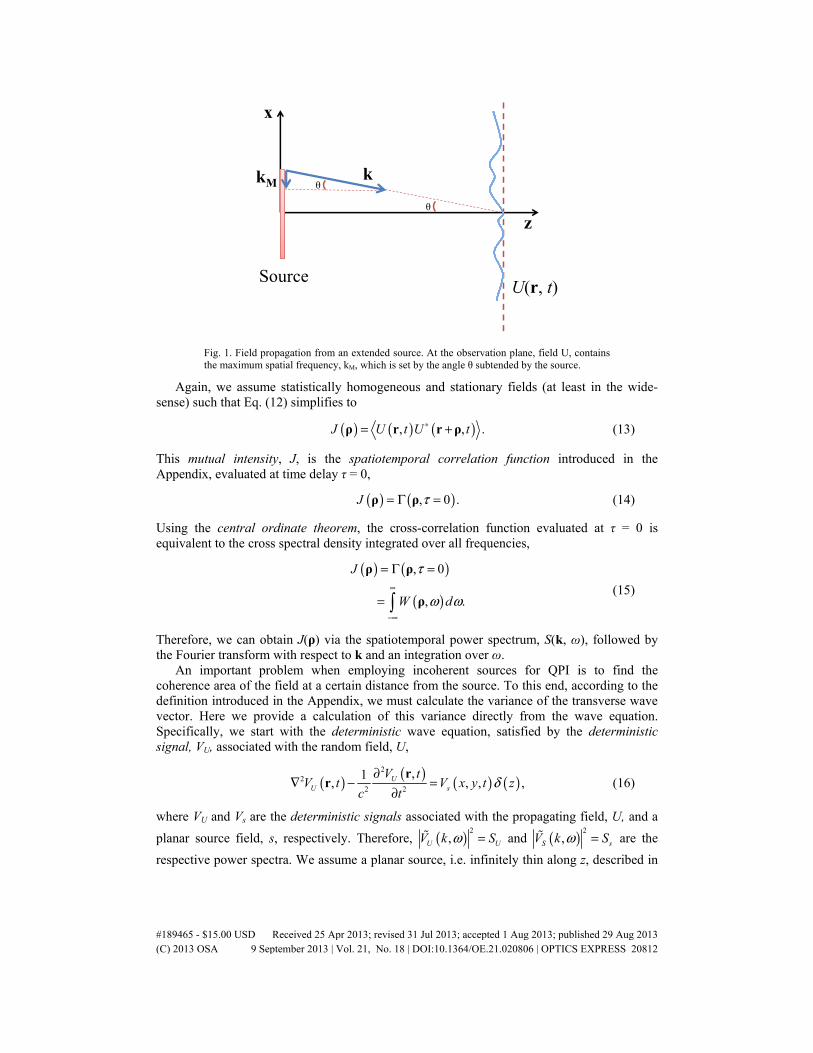
An important result in coherence theory is attributed to van Cittert and Zernike (see Section 4.4.4. in Mandel and Wolf [1]). This result is known as the van Cittert-Zernike theorem which establishes the spatial autocorrelation of the field radiated in the far-zone by a completely incoherent source (Fig. 1).

This result was originally formulated in terms of the mutual intensity, defined as

( ) ( ) ( )1 2 1 2, , , , .J t U t U t∗=r r r r (12)

In Eq. (12), the angular brackets indicate ensemble averaging over a certain area of interest (we are interested in the field distribution in a plane, r1,2∈ℜ2). This function J describes the spatial similarity (autocorrelation) of the field at a given instant, t, and it has been used commonly in statistical optics (see, e.g., [2].). The theorem establishes a relationship between J at the source plane and that of the field in the far zone. Such propagation of correlations has been described in detail by Mandel and Wolf [1]. Here, we derive the coherence area in the far-zone using the concept of the deterministic signal associated with a random field, as follows.


θ

k

U(r, t)

z

x

θkM

Source

Fig. 1. Field propagation from an extended source. At the observation plane, field U, contains the maximum spatial frequency, kM, which is set by the angle θ subtended by the source.

Again, we assume statistically homogeneous and stationary fields (at least in the wide-sense) such that Eq. (12) simplifies to

( ) ( ) ( ), , .J U t U t∗= +ρ r r ρ (13)

This mutual intensity, J, is the spatiotemporal correlation function introduced in the Appendix, evaluated at time delay τ = 0,

( ) ( ), 0 .J τ= Γ =ρ ρ (14)

Using the central ordinate theorem, the cross-correlation function evaluated at τ = 0 is equivalent to the cross spectral density integrated over all frequencies,

( ) ( )

( )

, 0

, .

J

W d

τ

ω ω∞

−∞

= Γ =

=

ρ ρ

ρ (15)

Therefore, we can obtain J(ρ) via the spatiotemporal power spectrum, S(k, ω), followed by the Fourier transform with respect to k and an integration over ω.

An important problem when employing incoherent sources for QPI is to find the coherence area of the field at a certain distance from the source. To this end, according to the definition introduced in the Appendix, we must calculate the variance of the transverse wave vector. Here we provide a calculation of this variance directly from the wave equation. Specifically, we start with the deterministic wave equation, satisfied by the deterministic signal, VU, associated with the random field, U,

( ) ( ) ( ) ( )2

22 2

,1, , , ,U

U s

V tV t V x y t z

c tδ

∂∇ − =

∂r

r (16)

where VU and Vs are the deterministic signals associated with the propagating field, U, and a

planar source field, s, respectively. Therefore, ( ) 2,U UV k Sω = and ( ) 2

,S sV k Sω = are the

respective power spectra. We assume a planar source, i.e. infinitely thin along z, described in


Eq. (16) by δ(z). By Fourier transforming Eq. (16), we readily obtain the solution in the ω−k domain [recall Eq. (9)]

( ) ( )2 20

,, ,S

U

VV

k

ωω

β⊥=

−k

k

(17)

where ( ),x yk k⊥ =k , 2 2 2 2x y zk k k k= + + , and 0 / cβ ω= . Next, we represent the propagating

field in terms of the variable z and 2 20 x yq k kβ= − − . Thus, using the partial fraction

decomposition,

2 2 2 20

1 1

1 1 1,

2

z

z z

k q k

q q k q k

β=

− −

= + − +

(18)

eliminating the negative frequency (inward) term, ( )1 zq k+ , we arrive at

( ) ( )( )

,, .

2S

Uz

VV

q q k

ωω ⊥=

−k

k

(19)

By Fourier transforming with respect to kz, we obtain the field UV as function of ⊥k and z,

which is known as the plane wave decomposition or Weyl’s formula (see, e.g., Section 3.2.4. in [1].),

( ) ( ), , , .2

iqz

U S

eV z iV

qω ω⊥ ⊥= −k k (20)

The modulus squared on both sides in Eq. (20), yields a z-independent relation in terms of the

respective power spectra, ( ) ( ) 2, , ,U U zS V zω ω⊥ =k k and ( ) ( ) 2

, , ,s s zS V zω ω⊥ =k k

( ) ( )2 20

1( ) , , .

4U sk S Sβ ω ω⊥ ⊥ ⊥− =k k (21)

If we assume that the spectrum of the observed field is centered at the origin, i.e., 0⊥ =k ,

and is isotropic, i.e., depends only on the magnitude of ⊥k , the variance can be simply

calculated as the second moment of k⊥ ⊥= k

( )( )

( )

2 2

2

2

,

,,

U

A

U

A

k S d

kS d

ωω

ω⊥

⊥

⊥ ⊥ ⊥

⊥⊥ ⊥

=

k

k

k k

k k (22)

where A⊥k is the ⊥k domain of integration. Thus, integrating Eq. (22) with respect to ⊥k , the

variance is obtained at once


( )( )

( )

2

2

220

2 20

,

,.

A

A

s

s

S d

kS

dk

ωβ

ω

β

ω ⊥

⊥

⊥ ⊥

⊥⊥

⊥

⊥

= −

−

k

k

k k

kk

(23)

We consider the source as fully spatially incoherent at all frequencies ω, i.e.,

( ) ( ),s sS Sω ω⊥ =k . Full spatial incoherence simplifies Eq. (23) to

( ) ( )2 2 2 2 2 20 01

k kA A

k d k k d kω β β⊥ ⊥

⊥ ⊥ ⊥ ⊥ = − − . Further, if we assume that the field of

interest is in the far zone of the source, which implies that 0k β⊥ << , then we can use the first

order Taylor expansion in terms of 0/k β⊥ , namely 2 2 2 2 20 0 01 / ( ) (1 / ) /k kβ β β⊥ ⊥− ≈ + . Finally,

the finite size of the source limits the spatial frequency in the far field by introducing a

maximum value of k⊥ , say Mk (see Fig. 1), such that 2 22 M

A A

d kdk kπ π⊥ ⊥

⊥ = = k k

k . Under

these circumstances, Eq. (23) simplifies to

2 2

0 2 20

2

11

1 / 2

/ 2,

M

M

kk

k

ββ⊥

= − + ≈

(24)

where we employed a Taylor expansion a second time. The maximum transverse wavevector can be expressed in terms of the half-angle subtended by the source, θ, because

0 sinMk β θ= . Thus, the coherence area of the observed field is

2

2

1 /

2,

cA k

λπ

⊥=

=Ω

(25)

where Ω is the solid angle subtended by the source from the plane of observation, 24 sinπ θΩ = .

This simple calculation captures the power of using deterministic signals associated with random fields as a means to reduce the coherence propagation equation from fourth-order in correlations to second-order in fields. Specifically, by taking the power spectrum of the solution, we were able to directly calculate the second moment of the transverse wavevector and implicitly obtain an expression for the spatial coherence of the propagating field. Equation (25) illustrates the remarkable result that, upon propagation, the field gains spatial coherence. In other words, the free-space propagation acts as a spatial low-pass filter. The farther the distance from the source, the smaller the solid angle Ω and, thus, the larger the coherence area.

4.2. Propagation of coherence from secondary sources

The concept of the deterministic signal associated with a random field can also be used to describe light propagation in inhomogeneous media, i.e., light propagation from a secondary source. Starting with the deterministic Helmholtz equation, the secondary source term can be separated to the right hand side.


( )22 2 2 2

0

20

( , ) ( , ) ( ) ( ) ( , )

( ) ( , ),

U U s

s

V V n n V

V

ω β ω β ω

β χ ω

∇ + = − −

= −r

r r r r r

r r (26)

where 0 / cβ ω= , 0 ( )nβ β=r

r , and 22( ) ( ) ( )n nχ = −r

r r r is the dielectric susceptibility.

Taking the spatial Fourier transform and separating the variables, the deterministic field propagation can be expressed in terms of the convolution of the secondary source and the initial incident deterministic field,

20

2 2 2

20

( , , ) ( ) ( , )( )

1 1( ) ( , ) ,

2

U z sz

sz z

V k Vk

Vq q k q k

βω χ ωβ

β χ ω

⊥⊥

= − − −

= − + + −

k

k

k k kk

k k

(27)

where k indicates a 3D convolution in the k-domain. Considering only the positive spatial

frequency component associated with zq k− , and taking the inverse Fourier transform in zk ,

the scattered deterministic field is,

20( , , ) ( , ) ( , , ) ,

2

iqz

U z s

eV z z V z

q

βω χ ω⊥ ⊥ ⊥ ⊥ = − k k k (28)

where z indicates convolution along z and ⊥ the 2D convolution along the transverse k-

vector, ( xk , yk ). The result can be simplified noting that the convolution of a function, f(z),

with a complex exponential yields a simple result, namely, ( ) ( )iqz iqzze f z e f q= , with ( )f q

the Fourier transform of ( )f z . Thus, Eq. (28) becomes

20( , , ) ( ) ( , ) .

2 z

iqz

U s k q

eV z V

q

βω χ ω⊥ = = − kk k k (29)

This is a remarkably simple result, which can be regarded as the first order Born scattering solution for an arbitrary illumination field. Equation (29) allows us to calculate, at any plane z, the power spectrum of the scattered field, which equals that of the respective

deterministic signal, 2

( , )UV ω⊥k , as a function of the illumination spectrum, 2

( , )sV ω⊥k ,

and the scattering potential, χ . Once we know the power spectrum, the frequency variances

can be evaluated directly as well. We illustrate these calculations by studying spatial and temporal coherence changes induced by scattering by biological tissues.

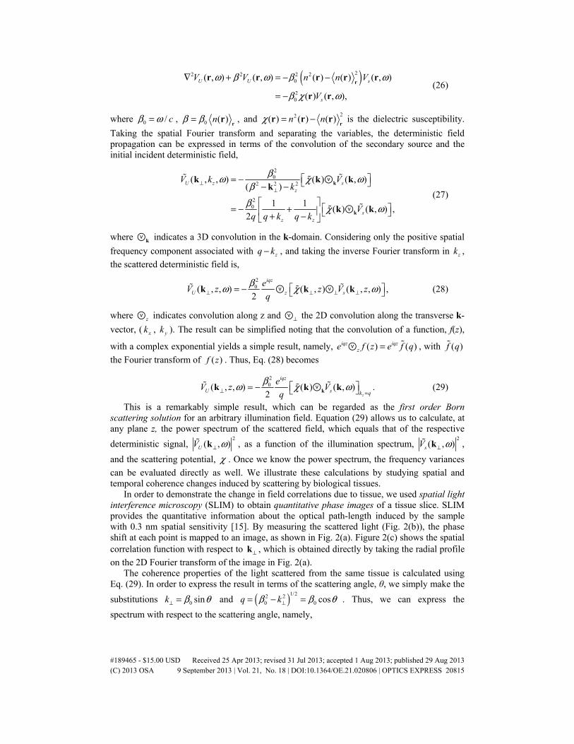
In order to demonstrate the change in field correlations due to tissue, we used spatial light interference microscopy (SLIM) to obtain quantitative phase images of a tissue slice. SLIM provides the quantitative information about the optical path-length induced by the sample with 0.3 nm spatial sensitivity [15]. By measuring the scattered light (Fig. 2(b)), the phase shift at each point is mapped to an image, as shown in Fig. 2(a). Figure 2(c) shows the spatial correlation function with respect to ⊥k , which is obtained directly by taking the radial profile

on the 2D Fourier transform of the image in Fig. 2(a). The coherence properties of the light scattered from the same tissue is calculated using

Eq. (29). In order to express the result in terms of the scattering angle, θ, we simply make the

substitutions 0 sink β θ⊥ = and ( )1/22 20 0 cosq kβ β θ⊥= − = . Thus, we can express the

spectrum with respect to the scattering angle, namely,


0

2

2 20

2 cos

( , ) ( , )

( ) ( , ) .4cos z

U

sk

S V

Vβ θ

θ ω θ ω

β χ ωθ =

=

= kk k

(30)

We study the spectral width of the scattered field with respect to the scattering angle. Based on the reciprocal relationship between the spectral linewidth and coherence time, 1τ ωΔ Δ ≈ , the coherence properties can be investigated. We define the width of the spectrum by its variance,

Fig. 2. (a) The optical path-length map of a tissue biopsy sample, imaged with SLIM using a 40X objective with 0.75 NA. A close-up of the sample is shown on the right as a demonstration of the imaging ability (quantitative and high-resolution). (b) The scattering geometry for this experiment. (c) The spectrum measured from sample shown in (a) through 2D Fourier transform and radial averaging. (d) Normalized optical spectrum for light propagated after the tissue. (e) The variation of effective spectral width of the angular spectrum.

( )2

2 0( ) ( , ).

( , )

U

U

S d

S d

ω ω θ ω ωω θ

θ ω ω

−Δ =

(31)

Assuming a Gaussian incident field spectrum centered at 7 11.3 10 rad m−× ⋅ with standard

deviation of 6 12 10 rad m−× ⋅ , Eqs. (30) and (31) yield the spectrum at each scattering angle and also the spectral bandwidth at each scattering angle. In Fig. 2(d), the resulting normalized spectrum of the calculation from Eq. (30) is shown with respect to the scattering angle. We can see a redshift in higher scattering angles due to the spatial correlation of the source as it is discussed in our previous paper [16]. Further, Fig. 2(e) shows the effective spectral width of


the angular spectrum that indicates the change of coherence time through a biological tissue with respect to the scattering angle.

5. Summary and discussion

We presented a new formalism for calculating propagation of field correlations using the wavevector-frequency representation of optical fields. The main points of this paper are as follows. 1) We first represent the coherence mode decomposition (CMD) in the wave-vector domain to prove that the plane waves can be used as an eigenfunction basis of the cross spectral density associated with statistically homogeneous fields. 2) We introduced the concept of a deterministic signal associated with a random field and showed that it significantly simplifies calculations of second order correlations. 3) We described spatial and temporal coherence in terms of the second order statistics (variance) of the spatial and temporal power spectra. Thus, for an arbitrary stochastic field, we can define a temporal bandwidth and coherence time for each spatial frequency (wavevector k) component and, vice versa, a spatial correlation for each temporal frequency ω. 4) We reviewed the stochastic wave equation in the Appendix and, for wide-sense stationary and statistically homogeneous fields, we solved this equation in the (k, ω) domain. Essentially, fourth order differential equations in field correlations can be replaced by second order differential equations for deterministic signals, which are defined via a Fourier transform of the spectral amplitude. These signals do not contain information about the spectral phase associated with the field. For example, the deterministic signal representation cannot make the distinction between a focused beam and a speckle field distribution with the same spatial bandwidth, or a light pulse versus a continuous wave field of the same temporal bandwidth. Therefore, it is important to note that the deterministic signal solution should only be used to generate the power spectrum (or autocorrelation) of the propagating field. From this power spectrum, first order (mean frequency) and second order (variance) statistics can be calculated both spatially and temporally, i.e., one can study how coherence changes upon propagation. 5) In Section 4, we applied the deterministic signal associated with a random field to derive a well-known result of the van Cittert-Zernike’s theorem, e.g., the field emitted by a spatially incoherent source gains coherence upon propagation. First we established that the mutual intensity, a quantity that is traditionally used for describing spatial coherence in a plane, is merely the frequency averaged cross-spectral density. This result allows us to easily calculate propagation of field correlations directly in the frequency (k, ω) domain. 6) If one is only interested to know the spatial and temporal variances, as measures of spatial and temporal coherence, we show that this second order statistics can be calculated straight from the wave equation in the frequency domain [e.g., Eq. (29)]. We illustrated this approach with correlations of fields propagating from primary and secondary sources.

Experimentally, we only have access to field correlations and not the fields themselves. Our results indicate that, for statistically translation-invariant fields, the deterministic signals give the same results as the actual (stochastic) fields. This explains why theoretical descriptions of interferometric experiments can yield the correct results even when randomness is ignored.

Appendix

A1. Stochastic wave equation

Here we review the propagation of field correlations from an arbitrary source that emits a random field s. We start with the scalar wave equation that has this random source as the driving term,

( ) ( ) ( )2

22 2

,1, , .

U tU t s t

c t

∂∇ − =

∂r

r r (32)


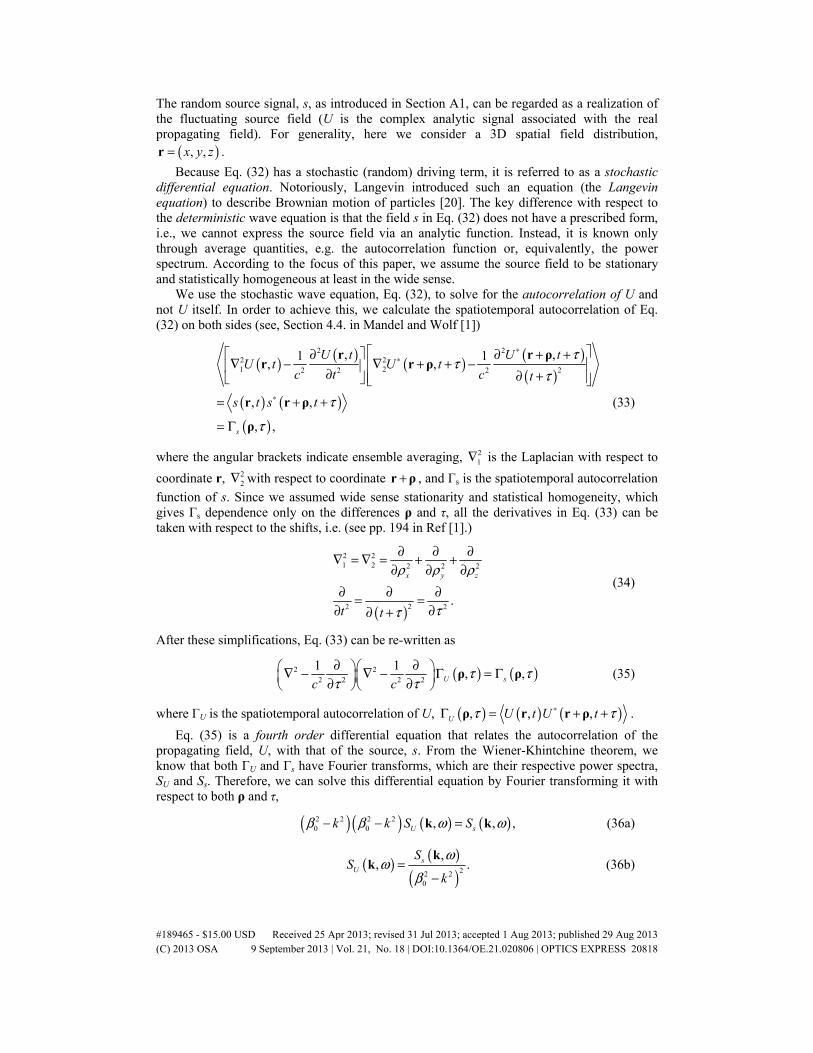
The random source signal, s, as introduced in Section A1, can be regarded as a realization of the fluctuating source field (U is the complex analytic signal associated with the real propagating field). For generality, here we consider a 3D spatial field distribution,

( ), ,x y z=r .

Because Eq. (32) has a stochastic (random) driving term, it is referred to as a stochastic differential equation. Notoriously, Langevin introduced such an equation (the Langevin equation) to describe Brownian motion of particles [20]. The key difference with respect to the deterministic wave equation is that the field s in Eq. (32) does not have a prescribed form, i.e., we cannot express the source field via an analytic function. Instead, it is known only through average quantities, e.g. the autocorrelation function or, equivalently, the power spectrum. According to the focus of this paper, we assume the source field to be stationary and statistically homogeneous at least in the wide sense.

We use the stochastic wave equation, Eq. (32), to solve for the autocorrelation of U and not U itself. In order to achieve this, we calculate the spatiotemporal autocorrelation of Eq. (32) on both sides (see, Section 4.4. in Mandel and Wolf [1])

( ) ( ) ( ) ( )( )

( ) ( )( )

2 22 21 2 22 2 2

, ,1 1, ,

, ,

, ,s

U t U tU t U t

c t c t

s t s t

ττ

τ

τ

τ

∗∗

∗

∂ ∂ + +∇ − ∇ + + − ∂ ∂ +

= + +

= Γ

r r ρr r ρ

r r ρ

ρ

(33)

where the angular brackets indicate ensemble averaging, 21∇ is the Laplacian with respect to

coordinate r, 22∇ with respect to coordinate +r ρ , and Γs is the spatiotemporal autocorrelation

function of s. Since we assumed wide sense stationarity and statistical homogeneity, which gives Γs dependence only on the differences ρ and τ, all the derivatives in Eq. (33) can be taken with respect to the shifts, i.e. (see pp. 194 in Ref [1].)

( )

2 21 2 2 2 2

22 2.

x y z

t t

ρ ρ ρ

ττ

∂ ∂ ∂∇ = ∇ = + +∂ ∂ ∂

∂ ∂ ∂= =∂ ∂∂ +

(34)

After these simplifications, Eq. (33) can be re-written as

( ) ( )2 22 2 2 2

1 1, ,U sc cτ τ

τ τ∂ ∂ ∇ − ∇ − Γ = Γ ∂ ∂

ρ ρ (35)

where ΓU is the spatiotemporal autocorrelation of U, ( ) ( ) ( ), , ,U U t U tτ τ∗Γ = + +ρ r r ρ .

Eq. (35) is a fourth order differential equation that relates the autocorrelation of the propagating field, U, with that of the source, s. From the Wiener-Khintchine theorem, we know that both ΓU and Γs have Fourier transforms, which are their respective power spectra, SU and Ss. Therefore, we can solve this differential equation by Fourier transforming it with respect to both ρ and τ,

( ) ( ) ( ) ( )2 2 2 20 0 , , ,U sk k S Sβ β ω ω− − =k k (36a)

( ) ( )( )22 2

0

,, .s

U

SS

k

ωω

β=

−

kk (36b)


In Eq. (36a), we used the differentiation property of the Fourier transform, i∇ → k ,

iωτ∂ → −

∂. Equation (36b) gives an expression, in the ω−k representation, for the spectrum

of the propagating field, SU, with respect to the spectrum of the source, Ss. Note that here the

function ( ) 22 20 kβ

−− is a filter function (transfer function), which incorporates all the effects

of free space propagation. Because the free space is isotropic, the transfer function is also isotropic, i.e., it depends only on the magnitude of the wavevector, k = k , and not its

direction.

A2. Coherence time and area

Let us consider the fluctuations of a field observed at a given plane. The coherence time, τc, and coherence area, Ac, describe the spread (standard deviation) of the autocorrelation function, ( ),τΛ ρ , in τ and ρ, respectively. Due to the uncertainty relation, τc and Ac are

inversely proportional to the bandwidths of their respective power spectra,

2 2 2

1,

1 1,

c

cx y

Ak k k

τω

⊥

=Δ

= =Δ Δ + Δ

(37)

where 2

2, , ,x y x y x yk k kΔ = − is the variance of the components of the transverse

wavevector, ( ),x yk k⊥ =k , and ,x yk their respective averages. Note that in this definition,

we assume that the statistical properties of the field are isotropic, meaning that the spatial coherence at a plane is characterized by a scalar function, Ac. If this is not the case, i.e., when the field statistics depends on direction, the coherence area is no longer sufficient and the

concept must be generalized to a tensor quantity, of the form, ( ), 1 / , , 1,2i j i jA k k i j= Δ Δ = .

The variances, 2ωΔ and 2xkΔ (similarly, 2

ykΔ ) are calculated explicitly using the

normalized power spectra as probability densities, namely

( )

( ) ( )

( )

( ) ( )

2

2

22

,

,

,

S d

S d

ωω

ω ω ω ωω

ω ω

ω ω

∞

⊥−∞

⊥ ∞

⊥−∞

⊥ ⊥

−Δ =

= −

k

k

k

k k

(38a)

( )

( )

( )

2 2

2

2

22

,

,

( ) ( ) .

x x

A

x

x x

k k S d

k

S d

k k

ωω

ω

ω ω

⊥

⊥⊥

⊥ ⊥

∞

⊥ ⊥−∞

−

Δ =

= −

k

kk

k k

k k (38b)

Clearly, the temporal bandwidth ( ) ( )2ω ω⊥ ⊥Δ = Δk k depends on the spatial frequency

⊥k . The physical meaning of a ⊥k -dependent coherence time is that each plane wave


component of the field can have a specific temporal correlation and, thus, coherence time,

( ) ( )1/cτ ω⊥ ⊥= Δk k . Conversely, each monochromatic component can have a particular

spatial correlation and, thus, coherence area, ( ) ( )21 /cA kω ω= Δ .

The two variances can be further averaged with respect to these variables, such that they become constant,

( ) ( )

( )

2 2

2

2

,

,

,

A

k

A

S d d

S d d

ω ω ω ω

ωω ω

⊥

⊥

⊥

∞

⊥ ⊥−∞

∞

⊥ ⊥−∞

−

Δ =

k

k

k k

k k

(39a)

( ) ( )

( )

2 2

2

2

,

.

,

x x

A

x

k k S d d

k

S d dω

ω ω

ω ω

⊥

∞

⊥ ⊥−∞

∞ ∞

⊥ ⊥−∞ −∞

−

Δ =

k

k k

k k

(39b)

Equation (39a) yields a coherence time, 21 /cτ ω= Δ , that is averaged over all spatial

frequencies, while Eq. (39b) provides a coherence area, 21 /cA k⊥= Δ , which is averaged

over all temporal frequencies. In practice, we always deal with fields that fluctuate in both time and space, but rarely do we specify τc as a function of k or vice-versa; we implicitly assume averaging of the form in Eq. (39a) and (39b).

Acknowledgments

This research was supported in part by the National Science Foundation (grants CBET 08-46660 CAREER, CBET-1040462 MRI). We acknowledge stimulating discussions with Prof. Scott Carney in our department. For more information, visit http://light.ece.illinois.edu/.


Date post:	13-Feb-2022
Category:	Documents
Upload:	others
View:	3 times
Download:	0 times

Deterministic signal associated with a random field

Documents