Page 1
DEVELOPING A CONSTRUCTION COST FUNCTION FOR
RESIDENTIAL BUILDINGS IN DHAKA CITY- AN ECONOMETRIC APPROACH
JOARDER MD SARWAR MUJIB
DEPARTMENT OF CIVIL ENGINEERING BANGLADESH UNIVERSITY OF ENGINEERING AND TECHNOLOGY
(BUET) Dhaka, Bangladesh
April, 20142015
Edited with the trial version of Foxit Advanced PDF Editor
To remove this notice, visit:www.foxitsoftware.com/shopping
Page 2
DEVELOPING A CONSTRUCTION COST FUNCTION FOR
RESIDENTIAL BUILDINGS IN DHAKA CITY- AN ECONOMETRIC APPROACH
By
Joarder Md Sarwar Mujib
A Thesis submitted to the Department of Civil Engineering of Bangladesh
University of Engineering and Technology, Dhaka in partial fulfilment of the requirements for the degree of
MASTER OF SCIENCE IN CIVIL ENGINEERING (STRUCTURAL)
DEPARTMENT OF CIVIL ENGINEERING BANGLADESH UNIVERSITY OF ENGINEERING AND
TECHNOLOGY (BUET)
Dhaka, Bangladesh
April, 20154
Edited with the trial version of Foxit Advanced PDF Editor
To remove this notice, visit:www.foxitsoftware.com/shopping
Page 3
CERTIFICATE OF APPROVAL The thesis titled “Developing A Construction Cost Function For Residential Buildings In Dhaka City-An Econometric Approach,” submitted by Joarder Md. Sarwar Mujib, Roll No. 1009042310, Session: Oct 2009, has been accepted as satisfactory in partial fulfillment of the requirement for the degree of Master of Science in Civil Engineering (Structural) on 4th April, 2015. Dr. Raquib Ahsan Chairman of the Committee Professor (Supervisor) Dept of Civil Engineering, BUET, Dhaka. Dr. A.M.M. Taufiqul Anwar Member Professor and Head (Ex-Officio)Dept of Civil Engineering,
BUET, Dhaka. Dr. Mahbuba Begum Member Professor Dept of Civil Engineering, BUET, Dhaka. Major Dr. Khondaker Sakil Ahmed Member Instructor Class B (External) Dept of Civil Engineering, Military Institute of Science and Technology (MIST), Dhaka
Edited with the trial version of Foxit Advanced PDF Editor
To remove this notice, visit:www.foxitsoftware.com/shopping
Page 4
DECLERATION
This is to certify this thesis work “Developing A Construction Cost Function For Residential Buildings In Dhaka City-An Econometric Approach” has been done by me. Neither of the thesis nor any part of has it been submitted elsewhere for the award of any degree or diploma.
Signature of the Candidate
Joarder Md. Sarwar Mujib
Edited with the trial version of Foxit Advanced PDF Editor
To remove this notice, visit:www.foxitsoftware.com/shopping
Page 5
Dedication To my Parents
Edited with the trial version of Foxit Advanced PDF Editor
To remove this notice, visit:www.foxitsoftware.com/shopping
Page 6
ACKNOWLEDGEMENT
I would like to express my heartfelt gratitude to Almighty Allah for all my
achievements.
I would like to articulate my gratitude to my present supervisor Dr. Raquib Ahsan, for
his encouragement and guidance of this research, without whose support, this research
work could never finish.
I would like to express my gratefulness to my Ex-supervisor Dr. Zia Wadud who
actually guided me to the concept and let me dream with such an exceptional research
topic. His direction and cordial support allowed me to complete the major part of the
research work.
I am grateful to Dr. Hadiuzzaman who assisted me with his valuable and convincing
suggestion in writing the paper in a befitting manner.
I will do injustice to this acknowledgements if I do not express my gratefulness to
Assistant Professor Kamrul Islam of MIST without whose inspiration and various
guidance probably I could not complete this paper.
I would like to express my sincere thanks to my committee members. Dr. A.M.M.
Taufiqul Anwar, Dr. Mahbuba Begum and Maj Dr. Khondaker Sakil Ahmed,
Engineers for their valuable advices, comments and supports. I strongly believe that I
was able to improve the paper and my knowledge further due to their insightful
comments.
I gratefully acknowledge the contribution of various authors who have been referred
in preparation of this thesis. My extended grateful acknowledgement to Damodar N.
Gujrati, Sangeetha, G.S. Maddala and C.R, Kothari whose books who have directly
helped me to develop the concept of the research and also the methodology by writing
Edited with the trial version of Foxit Advanced PDF Editor
To remove this notice, visit:www.foxitsoftware.com/shopping
Page 7
the books on Econometrics and Research Methodology.
I would like to express the recognition of my wife Umme Salma and my two
daughters Tahsinah Sarwar and Tahiyat Sarwar who have always inspired me
throughout the research.
Finally I like to acknowledge the contribution of the students of CE-11, CE-12 and
CE-13 of MIST who assisted me in data collection.
ABSTRACT
The preliminary cost estimate of a new building project is very significant which
provides the basis for the clients' budgeting, funding and controlling the project costs.
It is also the starting point on which the stakeholders decide whether to accept or
reject the project in question. A cost model should represent the significant cost items
in a form which will allow analysis and prediction of cost according to changes in the
design variables and price of cost elements. Only then it can be utilized in the
decision-making process. Considering the above fact the main objectives of this
research is to identify the possible cost elements and developing a general cost
function for residential building at Dhaka city. The developed model is then validated
to be useful for future study in this regards.
For the above study primary and secondary data were collected from the developers
of Dhaka city and Bangladesh Bureau of Statistics respectively. Total three models
were formulated using multiple linear regression (MLR) on 85 data with 26
independent variables (IV) and construction cost per sq. ft as dependent variable
(DV). Model-1 integrated construction materials' cost and labour wage and explained
91.4% of variability with standard error 65.461. Model-2 incorporated only design
variables as IV and explained only 32.9% variability with standard error 185.938.
Model-3 took account of all the variables explaining an increase of 0.5% of variability
only. Sand and Paint cost with Mason wage could describe the construction cost,
whereas design related variables displayed little influence on the DV. Models and
variables were statistically significant below 5% level. All models met MLR
assumptions and found suitable after cross validation and sensitivity analysis. Hence it
Comment [ja1]: Please correct.
Edited with the trial version of Foxit Advanced PDF Editor
To remove this notice, visit:www.foxitsoftware.com/shopping
Page 8
is concluded that model with materials' cost and wage explain the DV better.
However, a discrepancy is observed here, as steel and cement were not found
statistically significant whereas, these cause the maximum cost in reality. Conversely,
sand and paint being smaller in cost is contributing in these models. Foundation and
Structural systems is more important cost contributor but these are not statically
significant in our case. Concrete Strength, Steel Grade did not show desired
indication as in reality. This discrepancy might be because of data being collected
from developers of various standards and in different time frames, when sudden rise
and fall of the materials' cost took place. At the end, it could be noted that an
estimated project cost is not directly calculated from project components rather an
approximate indication of the cost derived from minimum possible number of
variables.
TABLE OF CONTENTS
CERTIFICATE OF APPROVAL………………………………………………….ii
DECLARATION……………………………………………………………………iii
ACKNOWLEDGEMENT………………………………………………………….v
ABSTRACT…………………………………………………………………………vi
TABLE OF CONTENTS...................................................................................... vii
LIST OF APPENDICES........................................................................................ xiv
LIST OF TABLES................................................................................................. xv
LIST OF FIGURES.................................................................................................xiii
ABSTRACT............................................................................................................xviii
CHAPTER ONE
INTRODUCTION........................................................................................................1
1.1 General..............................................................................................................1
1.2 Background and Present State of The Problem.................................................2
1.3 Objectives..........................................................................................................6
1.4 Outcomes/Benefits of the Study........................................................................6
1.5 Scope...................................................................................................................7
1.6 Methodology.....................................................................................................7
1.7 Guides to the Thesis..........................................................................................8
Edited with the trial version of Foxit Advanced PDF Editor
To remove this notice, visit:www.foxitsoftware.com/shopping
Page 9
CHAPTER TWO
LITERATURE REVIEW............................................................................................9
2.1 Introduction.......................................................................................................9
2.2 Various Research..............................................................................................9
2.3 Conclusion.......................................................................................................15
CHAPTER THREE
RESEARCH METHOD.............................................................................................16
3.1 Approaches to the Research.............................................................................16
3.2 Outline of Methodology...................................................................................16
3.3 Desk Study.......................................................................................................17
3.4 Pilot Field Survey.............................................................................................17
3.5 Formulation of Research Questionnaire..........................................................18
3.6 Data Collection for Main Research..................................................................20
3.7 Sampling Method Sample Size........................................................................20
3.8 Historical Analysis of Cost and Data...............................................................21
3.9 Statistical Analysis...........................................................................................21
3.10 Model Development........................................................................................22
CHAPTER FOUR
THE THEORETICAL ASPECTS OF THE DATA ANALYSIS AND
DEVELOPMENT OF COST MODEL....................................................................23
4.1 Introduction......................................................................................................23
4.2 Regression Analysis.........................................................................................23
4.3 Simple Regression Model..............................................................................24
4.4 Multiple Linear Regression (MLR): An Overview.........................................24
4.5 Important Definitions and Clarifications.........................................................25
4.5.1 Descriptive
Statistics...................................................................................25
4.5.2 Inferential Statistics....................................................................................25
4.5.3 Estimation Statistics....................................................................................26
4.5.4 Confidence Intervals...................................................................................26
4.5.5 Parameter Estimation..................................................................................26
4.5.6 Hypothesis Testing Statistics......................................................................26
4.6 Assumptions of MLR Analysis and Relevant Tests........................................26
4.6.1 Note to SPSS...............................................................................................29
4.7 Decision Rules for Development of Cost Model……………….....................29
Edited with the trial version of Foxit Advanced PDF Editor
To remove this notice, visit:www.foxitsoftware.com/shopping
Page 10
4.7.1 Descriptive
Statistics...................................................................................29
4.7.2 Correlation Matrix......................................................................................30
4.7.3 Curve Fit.....................................................................................................31
4.7.4 Histogram and Box Plot..............................................................................32
4.7.5 Data Sorting and Finalizing........................................................................33
4.8 Decision Rule for Model Development………………....................................33
4.9 Data Processing and Analysis..........................................................................34
4.9.1 Methods of Linear Regression for The
Model............................................34
4.9.2 Mode of Analysis for Final Model.............................................................35
4.9.3 Test of Significance....................................................................................35
4.9.4 Approaches to Analysis of Final Model.....................................................36
4.10 General Information About Model-1...............................................................36
4.11 Model With Enter Method...............................................................................36
4.11.1 Interpretation of The Model........................................................................37
4.11.2 The Variables Considered in The Model....................................................38
4.11.3 Model Summary.........................................................................................38
4.11.4 ANOVA......................................................................................................38
4.11.5 Coefficient..................................................................................................38
4.11.6 Concluding Remarks of The Model by Enter Method...............................38
4.12 Model With Stepwise Regression....................................................................39
4.12.1 Interpretation of The Model........................................................................40
4.12.2 The Variables Considered In The Model....................................................41
4.12.3 Model Summary.........................................................................................41
4.12.4 ANOVA......................................................................................................41
4.12.5 Coefficient..................................................................................................41
4.12.6 Practical Significance.................................................................................42
4.12.7 Concluding Remarks of The Models With Stepwise Regression...............42
4.13 Model With Backward Elimination Method....................................................42
4.13.1 Interpretation of The Model........................................................................45
4.13.2 The Variables Considered In The Model....................................................45
4.13.3 Model Summary.........................................................................................45
4.13.4 ANOVA......................................................................................................46
4.13.5 Coefficient..................................................................................................46
4.13.6 Practical Significance.................................................................................46
4.13.7 Concluding Remarks of the Models with Backward Elimination..............46
4.14 Model with Forward Selection Method...........................................................46
4.14.1 Interpretation of the Model Output Derived From Forward Selection......48
Edited with the trial version of Foxit Advanced PDF Editor
To remove this notice, visit:www.foxitsoftware.com/shopping
Page 11
4.15 Concluding Remarks for Step 1………….......................................................48
4.16 Description of Step 2……...............................................................................49
4.17 Model with Backward Elimination Method....................................................49
4.17.1 Concluding Remarks of the Models with Backward Elimination..............51
4.18 Model with Forward Selection Method...........................................................51
4.18.1 Concluding Remarks of the Models with Backward Elimination..............53
4.19 Model with Backward Elimination Method.....................................................53
4.19.1 Concluding Remarks of The Models With Backward Elimination............55
4.20 Model With Forward Selection Method...........................................................55
4.20.1 Concluding Remarks of The Models with Forward Selection...................56
4.21 Model With Backward Elimination Method....................................................56
4.21.1 Concluding Remarks of the Models with Backward Elimination..............58
4.22 Model with Forward Selection Method...........................................................59
4.22.1 Concluding Remarks of the Models with Forward Selection.....................60
4.23 Final Conclusion...............................................................................................60
4.24 General Information about Model-2.................................................................62
4.25 Model Enter Method........................................................................................62
4.25.1 Interpretation of The Model........................................................................63
4.25.2 The Variables Considered In The Model....................................................63
4.25.3 Model Summary.........................................................................................64
4.25.4 ANOVA......................................................................................................64
4.25.5 Coefficient..................................................................................................64
4.25.6 Concluding Remarks of The Model By Enter Method...............................64
4.26 Model with Backward Elimination Method-........................................64
4.26.1 Interpretation of the Model.........................................................................71
4.26.2 The Variables Considered In the Model.....................................................71
4.26.3 Model Summary.........................................................................................72
4.26.4 ANOVA......................................................................................................72
4.26.5 Coefficient..................................................................................................72
4.26.6 Practical Significance.................................................................................72
4.26.7 Concluding Remarks of the Models with Backward Elimination..............72
4.27 Model with Forward Selection Method-..............................................73
4.27.1 Interpretation of The Model........................................................................74
4.27.2 The Variables Considered In The Model....................................................74
4.27.3 Model Summary and ANOVA...................................................................75
4.27.4 Coefficient..................................................................................................75
4.27.5 Practical Significance.................................................................................75
4.27.6 Concluding Remarks of The Models With Forward
Selection...................75
Formatted: Indent: Hanging: 0.25"
Formatted: Indent: Hanging: 0.25"
Edited with the trial version of Foxit Advanced PDF Editor
To remove this notice, visit:www.foxitsoftware.com/shopping
Page 12
4.28 Model with Backward Elimination Method-........................................75
4.28.1 Interpretation of The Model........................................................................82
4.28.2 The Variables Considered In The Model....................................................82
4.28.3 Model Summary.........................................................................................82
4.28.4 ANOVA......................................................................................................82
4.28.5 Coefficient..................................................................................................82
4.28.6 Concluding Remarks of The Models With Backward Elimination-
2.........83
4.29 Model with Forward Selection Method-2........................................................83
4.29.1 Interpretation of The Model........................................................................84
4.29.2 The Variables Considered In The Model....................................................84
4.29.3 Model Summary and ANOVA...................................................................84
4.29.4 Coefficient..................................................................................................84
4.29.5 Practical Significance.................................................................................84
4.29.6 Concluding Remarks of The Models With Stepwise Regression...............85
4.30 Model with Backward Elimination Method-3.................................................85
4.30.1 Interpretation of The Model........................................................................91
4.30.2 The Variables Considered In The Model....................................................91
4.30.3 Model Summary.........................................................................................91
4.30.4 ANOVA......................................................................................................91
4.30.5 Coefficient..................................................................................................91
4.30.6 Practical Significance.................................................................................92
4.31 Model with Forward Selection Method-3………………................................92
4.31.1 Interpretation of The Model........................................................................93
4.31.2 The Variables Considered In The Model....................................................93
4.31.3 Model Summary And ANOVA..................................................................93
4.31.4 Concluding Remarks of The Analysis With Design Variables..................94
4.32 General Information about Model-3................................................................94
4.32.1 Model Enter Method...................................................................................94
4.32.2 Interpretation of The Model And Concluding Remarks By Enter Method........96
4.32.3 Concluding Remarks of The Model By Enter Method...............................96
4.33 Backward Elimination Method-1.....................................................................96
4.33.1 Interpretation of the Model and Concluding Remarks by Backward
Elimination Method-1...............................................................................
109
4.33.2 Concluding Remarks of the Model by Enter Method...............................109
4.34 Forward Selection Method-1..........................................................................110
Formatted: Indent: Hanging: 0.25"
Edited with the trial version of Foxit Advanced PDF Editor
To remove this notice, visit:www.foxitsoftware.com/shopping
Page 13
4.34.1 Interpretation of The Model And Concluding Remarks By Forward
Selection Method-1...................................................................................
112
4.34.2 Concluding Remarks of The Model By Forward Selection Method-1.....112
4.35 Backward Elimination Method-1...................................................................113
4.35.1 Interpretation of The Model And Concluding Remarks By Backward
Elimination Method-2...............................................................................
125
4.35.2 Concluding Remarks of The Model By Backward Elimination Method-1...126
4.36 Forward Selection Method-2.........................................................................
126
4.36.1 Interpretation of The Model And Concluding Remarks By Forward
Selection Method-1...................................................................................
128
4.36.2 Concluding Remarks of The Model By Enter Method.............................128
4.37 Backward Elimination Method-3...................................................................128
4.37.1 Interpretation of The Model And Concluding Remarks By Backward
Elimination Method-3...............................................................................
140
4.37.2 Concluding Remarks of The Model By Backward Elimination Method-1.....140
4.38 Forward Selection Method-3......................................................................... 140
4.38.1 Interpretation of The Model And Concluding Remarks By Forward
Selection Method-3...................................................................................
142
4.38.2 Concluding Remarks of The Model By Forward Selection-3..................143
4.39 Backward Elimination Method-4...................................................................143
4.39.1 Interpretation of The Model And Concluding Remarks By Backward
Elimination Method-3...............................................................................
154
4.39.2 Concluding Remarks of The Model By Backward Elimination Method-3.....154
4.40 Forward Selection-4.......................................................................................156
4.40.1 Interpretation of The Model and Concluding Remarks By Forward
Selection Method-4...................................................................................
156
4.40.2 Concluding Remarks of The Model By Forward Selection-4..................156
4.41 Backward Elimination Method-5...................................................................156
4.41.1 Interpretation of The Model And Concluding Remarks By Backward
Elimination Method-2...............................................................................
167
Edited with the trial version of Foxit Advanced PDF Editor
To remove this notice, visit:www.foxitsoftware.com/shopping
Page 14
4.41.2 Concluding Remarks of The Model By Backward Elimination Method-1.....167
4.42 Backward Elimination Method-4...................................................................167
4.42.1 Interpretation of The Model And Concluding Remarks By Backward
Elimination Method-2...............................................................................
176
4.42.2 Concluding Remarks of The Model By Backward Elimination Method-1.....177
4.43 Backward Elimination Method-4...................................................................177
4.43.1 Interpretation of The Model And Concluding Remarks By Backward
Elimination Method-2...............................................................................
185
4.43.2 Concluding Remarks of The Model By Backward Elimination Method-1.....186
4.44 The Final Model.............................................................................................186
CHAPTER FIVE
EMPERICAL RESULTS AND DISCUSSIONS...................................................188
5.1 Introduction....................................................................................................188
5.2 Boxplot And Identification Of Outliers.........................................................188
5.2.1 Boxplot of 87 Data....................................................................................189
5.3 Histogram of DV............................................................................................189
5.4 Descriptive Statistics......................................................................................191
5.5 Explanation of Result from SPSS Output (Model-1).....................................192
5.5.1 Model Summary (Model-1)......................................................................192
5.5.2 Analysis of Variance (Model-1)...............................................................194
5.5.3 Coefficients...............................................................................................197
5.5.4 Collinearity Statistics................................................................................199
5.5.5 Residual Statistics.....................................................................................200
5.6 Histogram of Residuals..................................................................................203
5.7 Normal P-P Plot of Standardized Residual (Model-1)..................................204
5.8 Scatter Plot of Standardized Residuals..........................................................205
5.9 Validation of The Model................................................................................206
5.10 Sensitivity Analysis........................................................................................206
5.11 Explanation of Result from SPSS Output (Model-1).....................................209
5.11.1 Model Summary (Model-2)......................................................................209
5.11.2 Analysis of Variance (Model-2)...............................................................210
5.11.3 Coefficients (Model-2).............................................................................210
5.11.4 Residual Statistics.....................................................................................211
5.12 Histogram of Residuals..................................................................................211
5.13 Normal P-P Plot of Standardized Residual (Model-1)...................................212
5.14 Scatter Plot of Standardized Residuals...........................................................214
Edited with the trial version of Foxit Advanced PDF Editor
To remove this notice, visit:www.foxitsoftware.com/shopping
Page 15
5.15 Validation of the Model.................................................................................215
5.16 Sensitivity Analysis.......................................................................................215
5.17 Explanation of Result from SPSS Output (Model-1)………………….........216
5.17.1 Model Summary (Model-2)......................................................................216
5.17.2 Analysis of Variance (Model-2)...............................................................216
5.17.3 Coefficients (Model-2).............................................................................217
5.17.4 Residual Statistics.....................................................................................218
5.18 Histogram of Residuals..................................................................................219
5.19 Normal P-P Plot of Standardized Residual (Model-1)...................................219
5.20 Scatter Plot of Standardized Residuals..........................................................220
5.21 Validation of The Model................................................................................222
5.22 Sensitivity Analysis........................................................................................223
5.23 Discussion on Empirical Result…………………………………………….224
5.23.1 The Data...................................................................................................224
5.23.2 The Model…………………………………………………………….…224
5.23.3 Comparison of the Models……………………………………………...226
5.23.4 Overall Significance…………………………………………………….226
5.23.5 Individual Significance……………………………………………….....227
5.23.6 Testing of Assumptions………………………………………………...227
5.23.7 Residual Statistics……………………………………………………....228
5.23.8 Cross validation on Data……………………………………………..…229
5.23.9 Sensitivity Analysis……………………………………………………..230
5.23.10 Conclusions………………………………………………………....231
CHAPTER SIX
CONCLUSIONS AND RECOMMENDATIONS.................................................233
6.1 Introduction....................................................................................................233
6.2 Conclusion......................................................................................................235
6.3 Limitations of the Study…………………………………………………….236
6.4 Recommendation And Future Study..............................................................237
REFERRENCES......................................................................................................238
Edited with the trial version of Foxit Advanced PDF Editor
To remove this notice, visit:www.foxitsoftware.com/shopping
Page 16
LIST OF APPENDICES
APPENDIX-A (Survey on Residential Building-Dhaka) PART A......................241
APPENDIX-B (Survey on Residential Building-Dhaka) PART B......................245
APPENDIX-C (SPECIMEN OF SAMPLE DATA IN SPREADSHEET)….....247
APPENDIX-D (DESCRIPTIVE STATISTICS).................................................249
APPENDIX-E (PEARSON CORRELATIONS MATRIX)................................251
APPENDIX-F (BIVARIATE DATA ANALISIS AND CURVE FITTING)…259
APPENDIX-G (BOXPLOT AND HISTOGRAM).............................................307
APPENDIX-H (VALIDATION OF MODELS).................................................336
Edited with the trial version of Foxit Advanced PDF Editor
To remove this notice, visit:www.foxitsoftware.com/shopping
Page 17
LIST OF TABLES
Table 4.1 Variables Entered/Removed.................................................................36
Table 4.2 Model Summary...................................................................................36
Table 4.3 ANOVA................................................................................................36
Table 4.4 Coefficients..........................................................................................37
Table 4.5 Variables Entered/Removed.................................................................38
Table 4.6 Model Summary...................................................................................39
Table 4.7 ANOVA................................................................................................39
Table 4.8 Coefficients..........................................................................................39
Table 4.9 Variables Entered/Removed.................................................................42
Table 4.10 Model Summary...................................................................................42
Table 4.11 ANOVA................................................................................................43
Table 4.12 Coefficients..........................................................................................43
Table 4.13 Variables Entered/Removed.................................................................46
Table 4.14 Model Summary...................................................................................46
Table 4.15 ANOVA................................................................................................47
Table 4.16 Coefficients..........................................................................................47
Table 4.17 Model Summary...................................................................................49
Table 4.18 ANOVA................................................................................................49
Table 4.19 Coefficients..........................................................................................49
Table 4.20 Model Summary...................................................................................51
Table 4.21 ANOVA................................................................................................51
Table 4.22 Coefficients..........................................................................................52
Table 4.23 Model Summary...................................................................................53
Table 4.24 ANOVA................................................................................................53
Table 4.25 Coefficients..........................................................................................53
Table 4.26 Model Summary...................................................................................55
Table 4.27 ANOVA................................................................................................55
Table 4.28 Coefficients..........................................................................................55
Table 4.29 Model Summary...................................................................................56
Table 4.30 ANOVA................................................................................................57
Table 4.31 Coefficients..........................................................................................57
Table 4.32 Model Summary...................................................................................59
Table 4.33 ANOVA...............................................................................................59
Table 4.34 Coefficients..........................................................................................59
Table 4.35 Model Summary...................................................................................61
Table 4.36 ANOVA................................................................................................61
Comment [ja2]: There shouldn't be two tables with the same caption.
Edited with the trial version of Foxit Advanced PDF Editor
To remove this notice, visit:www.foxitsoftware.com/shopping
Page 18
Table 4.37 Coefficients..........................................................................................62
Table 4.38 Model Summary...................................................................................64
Table 4.39 ANOVA................................................................................................64
Table 4.40 Coefficients..........................................................................................65
Table 4.41 Model Summary...................................................................................72
Table 4.42 ANOVA................................................................................................72
Table 4.43 Coefficients..........................................................................................73
Table 4.44 Model Summary...................................................................................75
Table 4.45 ANOVA................................................................................................75
Table 4.46 Coefficients..........................................................................................76
Table 4.47 Model Summary...................................................................................82
Table 4.48 ANOVA................................................................................................82
Table 4.49 Coefficients..........................................................................................83
Table 4.50 Model Summary...................................................................................84
Table 4.51 ANOVA................................................................................................85
Table 4.52 Coefficients..........................................................................................86
Table 4.53 Model Summary...................................................................................92
Table 4.54 ANOVA................................................................................................92
Table 4.55 Coefficients..........................................................................................92
Table 4.56 Model Summary...................................................................................95
Table 4.57 ANOVA................................................................................................95
Table 4.58 Coefficients..........................................................................................95
Table 4.59 Model Summary...................................................................................97
Table 4.60 ANOVA................................................................................................98
Table 4.61 Coefficients........................................................................................100
Table 4.62 Model Summary.................................................................................111
Table 4.63 ANOVA..............................................................................................111
Table 4.64 Coefficients........................................................................................112
Table 4.65 Model Summary.................................................................................114
Table 4.66 ANOVA..............................................................................................115
Table 4.67 Coefficients........................................................................................117
Table 4.68 Model Summary.................................................................................128
Table 4.69 ANOVA..............................................................................................128
Table 4.70 Coefficients........................................................................................129
Table 4.71 Model Summary.................................................................................130
Table 4.72 ANOVA..............................................................................................131
Table 4.73 Coefficients........................................................................................133
Table 4.74 Model Summary.................................................................................143
Table 4.75 ANOVA..............................................................................................143
Edited with the trial version of Foxit Advanced PDF Editor
To remove this notice, visit:www.foxitsoftware.com/shopping
Page 19
Table 4.76 Coefficients........................................................................................143
Table 4.77 Model Summary.................................................................................145
Table 4.78 ANOVA..............................................................................................146
Table 4.79 Coefficients........................................................................................147
Table 4.80 Model Summary.................................................................................157
Table 4.81 ANOVA..............................................................................................157
Table 4.82 Coefficients........................................................................................157
Table 4.83 Model Summary.................................................................................159
Table 4.84 ANOVA..............................................................................................160
Table 4.85 Coefficients........................................................................................162
Table 4.86 Model Summary.................................................................................171
Table 4.87 ANOVA..............................................................................................171
Table 4.88 Coefficients........................................................................................173
Table 4.89 Model Summary.................................................................................180
Table 4.90 ANOVA..............................................................................................181
Table 4.91 Coefficients........................................................................................182
Table 5.1 Descriptive Statistics.....................................................................192
Table 5.2 Model Summary (Model-1)............................................................194
Table 5.3 ANOVA (Model-1).......................................................................196
Table 5.4 Coefficients (Model-1)...................................................................198
Table 5.5 Residuals Statistics (Model-1)...........................................................201
Table 5.6 Model Summary (Model-2)............................................................211
Table 5.7 ANOVA (Model-2).......................................................................211
Table 5.8 Coefficients..................................................................................212
Table 5.9 Residuals Statistics........................................................................213
Table 5.10 Model Summary (Model-3)...........................................................218
Table 5.11 ANOVA (model-3).......................................................................218
Table 5.12 Coefficients (model-3)...................................................................219
Table 5.13 Residuals Statistics (Model-3)..........................................................220
Table 5.14 Comparison of the Models.............................................................227
Edited with the trial version of Foxit Advanced PDF Editor
To remove this notice, visit:www.foxitsoftware.com/shopping
Page 20
LIST OF FIGURES
Figure 5.1 Boxplot of Construction Cost-87 Data............................................190
Figure 5.2 Boxplot of Construction Cost-85 Data..............................................191
Figure 5.3 Histogram of Construction Cost.....................................................192
Figure 5.4 Histogram of Residuals (Model-1)..................................................205
Figure 5.5 Normal P-P Plot of Standardized Residual (Model-1).......................206
Figure 5.6 Scattered Plot of Standardized Residual vs. Standardized Predicted
Value (Model-1)................................................................................. 207
Figure 5.7 Sensitivity Analysis of Model-1 Variables (DV vs IV).....................210
Figure 5.8 Histogram of Standardized Residuals (Model-2)...............................214
Figure 5.9 Normal P-P Plot of Standardized Residuals (Model-2).....................215
Figure 5.10 Scatter Plot of Standardized Residuals vs. Standardized Predicted
Value (Model-2).................................................................................215
Figure 5.11 Sensitivity Analysis of Model-2 Variables (DV vs. IV)....................217
Figure 5.12 Histogram of Standard Residuals (Model-3)......................................221
Figure 5.13 Normal P-P Plot of Standardized Residuals (Model-3).....................222
Figure 5.14 Scatter Plot of Standardized Residuals vs. Standardized Predicted
Value (Model-3)................................................................................223
Figure 5.15 Sensitivity Analysis of Model-3 Variables (DV vs. IV)...................224
Edited with the trial version of Foxit Advanced PDF Editor
To remove this notice, visit:www.foxitsoftware.com/shopping
Page 21
CHAPTER ONE
INTRODUCTION
1.1 Introduction
Any prospective client who is interested in building a structure would first ask the
question “How much will the project cost?” Naturally the next question would be
“how accurate is this figure as answered in response to the first question?" The
preliminary cost estimate of a new building project remains a benchmark throughout
the project period. This estimate provides the basis for the constructor's (a developer,
an agency or an individual) budgeting, funding and controlling the construction costs.
This is also the starting point on which the stakeholders decide whether to accept or
reject the project in question. At the same time a client who is interested to purchase
the whole or a part of the building would also be interested to know the same as to
how far he will bargain for the price. Again a land owner who is interested to get his
building constructed in joint venture with a developer will also be interested in the
same question as to fix the signing money and percentage of his share. A bidder who
prepares himself to get a similar contract by bidding is also required to prepare the
minimum and maximum price he may have to spend for the project. All these
institutions, agencies and individuals primarily focus on the answers of these two
questions. However, regular construction experiences reveal that purely prediction
sometimes ends up in non-pragmatic conclusions.
Cost modeling may be defined as the symbolic representation of a system in terms of
the factors, which influence its cost. In other words, a model represents the significant
cost items of a building in a form which will allow analysis and prediction of cost to
be undertaken according to changes in the design variables and direct cost elements.
The idea is to prepare a model such that it would simulate both current and future
situations and the problems of early cost estimation may be taken care of, thereby, it
can be used in the decision-making process.
1.2 Background and Present State of the Problem
Edited with the trial version of Foxit Advanced PDF Editor
To remove this notice, visit:www.foxitsoftware.com/shopping
Page 22
Dhaka - the Capital city of Bangladesh is known to be one of the most populated
megacities of the world. The residential areas are gradually adapting the dynamic
changes in patterns for rapid growth of the city population. However, these areas have
lost much of their residential characteristics in order to cope with rapid urbanization.
The traditional urban housing system in Dhaka has undergone many radical
transformations over the past few decades. The continuous growth has given scope of
large scale housing project in and around the city. As a result huge private developers
have emerged to take the opportunity and construct medium to high rise buildings to
meet up the scarcity of accommodations. The major clients are higher middle class to
upper class of the society. The location and importance of nearby features have a
great effect of valuation perception both for the people as well as the developers. The
developers generally undertake projects through mutual agreements with land owner
rather than purchasing land. A decision is often required to be taken by the clients/
land owners whether they should agree to the proposal of the developers. Naturally,
the question comes in mind of the prospective client or land owner “Is their cost
perception about the project reasonable? Or “Are the developer’s bargain
acceptable?”
A building project can only be regarded as successful, once it is delivered in time, at
the appropriate price and quality providing the client with a high level of satisfaction.
One important influence on this is the authenticity of the cost estimates prepared
during the various phases, especially in the conception phase. Often the quality of the
project, along with the ability to construct and complete on schedule largely depends
on the accuracy of cost estimates made in the design phase. Since cost has been
identified as one of the measures of function and performance of a building, it should
be capable of being modeled so that a tentative design can also be indicated. This will
assist in providing greater understanding and possibility of predicting the cost effect
for changing the design variables.
It is clear that, early cost estimates are accepted as approximations that includes some
degree of uncertainty. If it is too high then it may discourage the prospective client
from proceeding further with the scheme. Conversely, if the estimate is too low, it
may result in wasted development efforts, dissatisfaction on the part of the client,
such as obtaining lower than expected returns or even litigation.
Edited with the trial version of Foxit Advanced PDF Editor
To remove this notice, visit:www.foxitsoftware.com/shopping
Page 23
The principal components of the cost of any construction facility include the market
prices of construction materials and the wage agreements. Besides these, few design
parameters like foundation types, structural forms, slab systems etc also involve cost
as they occupy additional costs in terms of materials and labour wage. Design
variables like concrete strength, steel reinforcement grade, plinth area, number of
stories, size of lobby, number of basements, number of stairs and number of toilets
also contribute some variations in cost. Other parameters like plumbing and electrical
system (Transformer, generator and lift capacity), location and accessibility, time and
season, climatic conditions, availability and interest rates of capital, demand for
construction, political and economic climates etc. also incur variations in cost. While
several of these factors could be constant for a given project, the design style still
could be varied in order to select the most economical option. It is in fact customary
that for any project, the designer will make liaison with the client considering several
economical design solutions. The factors that have economic consequences in various
design options are identified and examined, and thus, these often form the basis of
selecting the most suitable and appropriate proposal for the prospective client to
embark upon.
There have been sporadic attempts to develop cost models in Bangladesh and other
countries. These include efforts in U.S.A.(Texas), Nigeria, UK, Korea, Turkey,
Australia and a few more countries. The scope and purpose of research, modeling
methodology, data used and geographic coverage vary significantly from each other
in all these studies. It is particularly noticeable that, there has not been sufficient
research that provides any correlation or clear indications of the degree to which
changes in the construction parameters of the building (materials' cost and design
variables) would affect its cost with regards to Dhaka city.
In our country a few government organizations like Public Works Department
(PWD), Military Engineering Services (MES), Local Government Engineering
Department (LGED), City Corporation prepare schedule of rates for their own
buildings at the interval of five to ten years. Each organization makes some
amendments as the price of construction materials, labour wage and cost of
machineries change. MES prepare the cost estimate of individual item (work) per unit
volume which includes cost of materials, labour, income tax, value added tax and
contractors profit, also a few other cost adding some additional percentages. They
Edited with the trial version of Foxit Advanced PDF Editor
To remove this notice, visit:www.foxitsoftware.com/shopping
Page 24
make contracts of any building by referring the cost per unit volume/ area of each
item as applicable. If any part of the integrated cost changes between the approvals of
the two consecutive schedules of rates, re-fixing is not possible without going to the
origin of cost. A few more estimating techniques used in our country at the pre-design
phase of the construction project do not seem to have any fixed procedure. Small to
medium firms take account of their recently completed project and make some
adjustment on cost with additional cost of 10% to 25% as unforeseen. Only the
renowned firms make the cost estimation based on design and quantity surveying by
preparing a Bill of Quantity (BOQ). If any changes take place in terms of only a
single design variable such as foundation, floor system, structural forms etc. each time
the firms have to redesign and calculate the BOQ separately time and again. This
eventually results in additional time and cost of overall design. Nobody follows a
unique tool to make a quick estimate considering all design variables and functional
parameters. Few developers use Microsoft Project to control their construction
project. It is not possible for anybody other than an engineer, who has adequate
knowledge on the construction process to involve in the above procedure stated. At
the same time a statistician who is interested to study the trends of construction cost
for drawing macroeconomic inference will not be able to follow the existing
procedure without having prior knowledge of construction engineering.
The cost model may be considered satisfactory to the researcher if the variation
generates on application is within the acceptable economic tolerance limit. The
probable cost function that would be identified in this research involves all possible
cost items and design variables and makes a generalized equation. Most interesting
aspect of this model is that, the estimators have options to change any design
variables at any stage and amend the estimated cost. At the same time, persons
without having the adequate knowledge on building may estimate the cost. The model
is expected to be more versatile and fits the residential buildings with almost all types
of design parameters. It is also expected that the multiple regression model, planned
for the present research, may unfold a new avenue for the researchers of Bangladesh
for making further study with both numerical and categorical design variables to
develop any cost function for Bangladesh in particular. Present study is carried out
with only panel data. But this approach can be used for both Time Series and Pooled
Edited with the trial version of Foxit Advanced PDF Editor
To remove this notice, visit:www.foxitsoftware.com/shopping
Page 25
data also. This model can be effectively planned for cost function of other disciplines
also.
Econometrics, the result of a certain outlook on the role of economics,
consists of the application of mathematical statistics to economic data to
lend empirical support to the models constructed by mathematical
economics and to obtain numerical results. The art of the
econometrician consists in finding the set of assumptions that are both
sufficiently specific and sufficiently realistic to allow him to take the best
possible advantage of the data available to him. Linear Regression is the
most important tool of Econometrics and multiple regression provides a
powerful method to analyze multivariate data creating linear function of the cost
variables. Construction cost involves huge numbers of independent variables. To deal
with these massive variables Bill of Quantity (BOQ) method is very prolonged and
also burdensome. More so, it is not comprehensible for the people not concerned in
construction. There are many who are interested to know the cost but have no
opportunity to conceptualize the matter. Hence, if a researcher make it usable by all
stakeholders, it will be a unique one and very effective for the mass people.
Regression analyses are usually driven by a theoretical or conceptual model that can
be drawn in the form of a path diagram. The path diagram provides the model for
setting the regression and what statistics to examine. If one assumes linear relations
between variables, it provides a ‘road map’ to a set of theoretically guided linear
equations that can be analyzed by multiple regression methods. Multiple regression is
widely used to estimate the size and significance of the effects of a number of
independent variables on a dependent variable. Before a complete regression analysis
can be performed, the assumptions concerning the original data must be made.
Ignoring the regression assumptions contribute to wrong validity estimates. When the
assumptions are not met, the results may upshot in errors, or over- or under-estimation
of significance of effect size. Meaningful data analysis relies on the researcher’s
understanding and testing of the assumptions and the consequences of violations. The
old research shows that the researchers are drawing their own conclusions after testing
the assumptions and results of the statistical tests.
Edited with the trial version of Foxit Advanced PDF Editor
To remove this notice, visit:www.foxitsoftware.com/shopping
Page 26
1.3 Objectives
The aim of this research is to study the residential building construction cost to
develop an early cost estimating construction cost model for Dhaka city. The specific
objectives are:
To identify all possible cost elements of the residential building construction.
Developing a general construction cost function for residential building at
Dhaka city for pre-design construction project cost predictions.
To validate the model as how it explains the unit cost (construction cost per
square feet) in other words to verify the effectiveness of the model.
1.4 Outcomes/Benefits of the Study
The benefits which could be derived from the research are as follows:
The model when developed is going to facilitate the method of predicting pre-
design construction cost for anybody who have no or little knowledge about
the construction process. Probably it is going to establish the first ever initial
cost predicting model for construction cost in Bangladesh by an econometric
approach, basing on which other researchers can develop other cost predicting
models.
The research is going to unveil some of the factors that affect construction
cost, and hence will draw estimator's attention to inculcate the effects of those
factors in their initial estimates to nullify or reduce the end effects.
The research findings also serves as the researcher's contribution to existing
knowledge, and should form the basis for other related further research works.
The expected outcome of the present study would be beneficial to estimate the
probable cost of construction per square foot during inception phase by the
stakeholders (constructors, developers, land owner, government agencies,
researcher etc.).
To identify the design variables (numeric and non numeric) those have the
largest effect or have no or little effect on total cost.
Edited with the trial version of Foxit Advanced PDF Editor
To remove this notice, visit:www.foxitsoftware.com/shopping
Page 27
1.5 Scope
This work seeks to find out a quick estimation method to be used by different
stakeholders interested in predicting the initial pre-design construction cost. The
scope of the research is limited to only Reinforced Cement Concrete (RCC) buildings
in Dhaka city. The primary data were collected from developers and secondary data
were obtained from Statistical Year Book. Variation in quality of materials and
workmanship is not considered here. For interpreting secondary data, few
construction engineering judgments were made which may vary in reality. Cost of
materials, assumed/collected, was considered as constant, although it may vary over
the project duration for some materials. The research has been carried out purely on
available data which was sorted out on the basis of engineering judgment and market
study. Monetary value of cost of materials and other expenditure was perceived in the
accounting scale. Time value of money such as bank interest and other miscellaneous
cost was not taken into consideration.
1.6 Methodology
The research is planned to employ an econometric modeling approach for developing
a general cost function equation for residential building at Dhaka city. Almost 275
building projects data with more than 100 variables were collected. However after
scrutiny, only 25 variables have finally been considered for the study. The data were
sorted in spread sheet and finally 206 data sets have been selected for the research.
Multiple regression analysis has been adopted as it is most suitable for analyzing
these types of data set. The statistical software SPSS and MS Excel 2007 were used as
the tools for this research. In the proposed study primary cross-sectional data were
collected from different developers who construct residential building at Dhaka.
Initially a pilot project was carried out to identify the issue and finally a full survey
was conducted. At first all probable cost elements were identified by the pilot project
and from that, final survey questionnaires were prepared. There are both qualitative
and quantitative variables. Few of the potential variables are price of construction
materials, total plinth area, foundations types, structural form, floor system, locations
etc. An appropriate econometric model was developed using the SPSS platform.
Relevant statistical tests were carried out to determine the best possible model.
Edited with the trial version of Foxit Advanced PDF Editor
To remove this notice, visit:www.foxitsoftware.com/shopping
Page 28
1.7 Organization of the Thesis
The thesis was presented in Six (6) chapters as follows:
Chapter1: gives the introduction which also includes background of the research,
outlines the aims and objectives. It also states the benefits, scope and method of the
research briefly.
Chapter 2: presents the available literature on the various methods of initial cost
predictions and basic approaches to cost estimation.
Chapter 3: presents the methodology and shows the general approach to the research.
Chapter 4: gives the general overview of the principle of regression analysis and its
application in the model development. This chapters also shows the research data
analysis process and steps to empirical model development
Chapter 5: presents the optimized result with descriptive statistics concerning the
variables associated with final empirical model. This chapter also shows the
discussion of the result found.
Chapter 6: contains the conclusions drawn from the research, the researcher's
contribution to knowledge and recommendations for further research.
Edited with the trial version of Foxit Advanced PDF Editor
To remove this notice, visit:www.foxitsoftware.com/shopping
Page 29
CHAPTER TWO
LITERATURE REVIEW
2.1 Introduction
Construction cost estimation is one of the most challenging responsibilities in order to
ensure proper allocation of funding resources among different phases and events of
construction. It plays a vital role in decision making process of various stakeholders
such as owner, contractors, sub-contractors, designer, consultants etc. Thus the
successful completion and extent of a construction project largely depend on initial or
conceptual cost estimation. Previous researches emphasize on the accuracy of
conceptual cost estimation. Various approaches namely Regression Analysis, Neural
Network, Case Based Reasoning were adopted by different research groups to
minimize the gap between estimation and final project cost. A large number of
variables related to project thus introduced by the authors to incorporate maximum
uncertainties and deviation of the real project. Some of these variables are highly
sensitive to location of the project. Literature review reveals some study in the context
of U.K, USA, Nigeria and Turkey etc. But similar study related to Bangladesh in
particular Dhaka being the one of the most populated city is neither conducted nor
effort was taken. That is why; the necessity of development of a cost estimation
model in the context of Bangladesh is then initiated in order to incorporate local
project related variables.
2.2 Various Researches
Khosrowshahi and Kaka (1996), Lowe et al. (2006), Kantanantha and Leelakriangsak
(2012), Skitmore and Thomas Ng (2003), Ganiyu and Zubairu (2010), Hollar et al.
(2010) used the regression model to predict the cost of different construction project
in terms of different variables. However, the limitations of the regression model were
studied by Kim et al. (2004), Amusanet et al. (2013), Jamshid Sodikov (2005) as a
comparative approach. Their study concluded that Neural Network can estimate the
cost more accurately than that of the traditional Regression Analysis. Khosrowshahi
and Kaka (1996) describes a simple predictive model for estimation of project cost
Edited with the trial version of Foxit Advanced PDF Editor
To remove this notice, visit:www.foxitsoftware.com/shopping
Page 30
and duration of U.K. housing project. The predictive model is based on regression
analysis by iteration contain predictors which based on their statistical performance.
Cost and duration were separately evaluated through two different models where the
cost model was independent of duration model. Hollar et al. (2010) describe an
approach for the development of a regression model to predict preliminary
engineering costs. Study result shows that, multiple linear regressions modeling also
show promises as a tool that support improvement in PE estimate preparation as well
as cost budgeting which can be used for effective distribution of funding resources to
capital project. Ganiyu and Zubairu (2010) identifies six most important design
related variables as complexity in design and construction, advancement in
technology, percentage of repetitive element, special issues and scope of work to
affect the ultimate project cost. Time given by the client for bid evaluation,
importance of project to be delivered and the need for the project completion are three
main time/cost related factors. Beside this, contractors and consultants previous
experience and adequacy of plant and equipment’s also plays significant role for
project cost estimation model. The factors were then incorporated in the predictive
cost model using principle components regression analysis. Later Lowe et al. (2006)
shows that multiple regression techniques can be more effective to predict the
construction cost of buildings rather than the traditional methods of cost estimation. In
their study the regression models were developed for cost\m2, log of cost and log of
cost\m2 rejecting the raw costs. Total six models were obtained by performing both
forward and backward stepwise analyses. Throughout the models total 19 different
variables were used. Among all six models log of backward model is considered as
the best one that gives an R2 of 0.661 and MAPE of 19.3%. The data used in the
model were collected from 286 United Kingdom construction projects. In another
study, Lowe et al. (2007) establishes a relationship among the project strategic, site
related and design related variables with the total construction cost. The study uses
data of 286 construction project in U.K. which were then validated using regression
analysis and neural network cost models. Use of different regression techniques were
observed in the study of Skitmore and Thomas Ng (2003). They describe the
deviation of the actual construction time and cost of construction project from the
contract time and cost. A set of 93 Australian construction projects were used to
develop several models for actual construction time and cost prediction. Different
analysis like forward regression, Standard cross-validation regression was conducted
Edited with the trial version of Foxit Advanced PDF Editor
To remove this notice, visit:www.foxitsoftware.com/shopping
Page 31
to develop a model for forecasting actual construction time when client sector,
contractor selection method, contractual arrangements, project type, contract period
and contract sum are known. Then the sensitivity analysis of the model was done
since the prediction of actual construction time and cost is based on the estimated
contract period and contract sum. After that, the practical application was examined
by plotting different curves that helps the client to select the perfect project type to
minimize the variation between actual and contract time and cost.
Li et al. (2005) made an endeavor to develop a regression cost model for office
buildings in Hong Kong to predict the cost estimation at initial stage of any
construction project. Multiple regression analysis involving few variables had been
done to develop cost modeling. Historical data of 37 office buildings in Hong Kong,
constructed in different years, had been collected to develop the cost model that
included detailed information on the final construction cost, average floor area, total
floor area, average storey height, total building height, number of storey above
ground, number of basements and types of construction. The final construction cost
data were adjusted by the construction price index and categorized as dependent
variable while the rest data were categorized as independent variables. The
relationship between the final construction cost and the independent variables was
made by using the computer software (SPSS-17 package) to find the most accurate
equation. 7 samples out of 14 reinforced concrete buildings and 11 samples out of 23
steel buildings were randomly selected for verifying the result. Result shows that total
floor area and total building height entered into the final regression model equation
and resulted in more than 96% of the accuracy for reinforced concrete office
buildings. Total floor area, average floor area and total building height remained in
final equation and yielded over 95% of accuracy for steel office buildings. The major
limitation of the study was that, it was only considered for office buildings in Hong
Kong. But the research methodology is universal which can be applicable for other
residential and non-residential buildings as well. The reliability of the cost models
could be further enhanced by inclusion of more number of buildings. Continuous
updating the data can be a possible option to meet the future trend which is changing
frequently due to dynamic nature of construction industry.
Edited with the trial version of Foxit Advanced PDF Editor
To remove this notice, visit:www.foxitsoftware.com/shopping
Page 32
In a different study on cost estimation of electrical and communication system for
industry Kantanantha and Leelakriangsak (2012) describes three different
methodologies namely Multiple Regression Analysis (MRA), Multiple Regression
Analysis Incorporating Genetic Algorithm (MRA-GA) and Neural Network. Result
shows that the electrical and communication system is composed of ten sub-systems
and the cost can be classified into five main components. The floor area and provision
of Air conditioning systems are considered as input variables and the cost as output
variable. Accuracy of the methods is measured by Root mean Squared Error (RMSE)
and the MRA-GA model provides a little lower RMSE than other two models.
Though MRA-GA model provides lower RMSE but it doesn’t prove it as the best
technique. Rather MRA-GA and NN technique takes time to develop whereas the
MRA is quick is providing the result. In his study Kim et. al. (2004) presented a
comparative study on the performance of three different construction cost estimation
models based on multiple regression analysis (MRA), neural network (NN) and the
case based reasoning (CBR) with respect to the data of 530 historical cases. Result
shows that the NN estimating model was more accurate than other two methods
whereas the CBR shows better performance considering long term use, availability of
information from result and time versus accuracy tradeoffs. Amusan et al. (2013) uses
the Artificial Neural Network (ANN) model to estimate the construction cost of
building projects. Their study shows that the neural network model is more accurate
than the traditional regression analysis with a maximum range variation of 7.42
percent. The corruption escalator factor and the inflation buffer factors were included
in the model for obtaining the actual performance of the model. A similar study of
Jamshid Sodikov (2005) suggested that, in the conceptual phase of a project the cost
estimation usually calculated on approximation and it leads to a great inaccuracy.
ANN could be a useful tool to help solve problems which come from the cost
estimation at the conceptual phase. Therefore, the development of an ANN model of
cost estimation should be focused by incorporating methods like Fuzzy Logic, Case
Based Reasoning etc.
However some other methodologies were also adopted by many researchers. For
instance, Cheng et. al. (2010) constructed an evolutionary estimate at completion
(EAC) model to estimate the final cost of the project based on the evolutionary
support vector machine interface model (ESIM). The two artificial intelligence
Edited with the trial version of Foxit Advanced PDF Editor
To remove this notice, visit:www.foxitsoftware.com/shopping
Page 33
approaches fast messy genetic algorithm (FMGA) and support vector machine (SVM)
were merged to generate the ESIM model. The probable project performance and
risks associated with the project are taken into consideration to construct the EAC
model and hence the performance of the model was found satisfactory which was
validated using real applications. Somerville (1999) introduces a new set of micro-
data on housing construction cost to construct the quality controlled, hedonic cost
series based on this data set. Result shows that, the hedonic cost series can better
estimate the supply of new single family housing than the existing housing supply
studies. The study also shows that housing starts are cost elastic and the endogenous
behavior of the construction cost in the new housing supply functions. Skomrlj and
Radujković describes the S-curve methodology to establish a relationship between the
project cost and duration of the project based on 24 terminated high rise building
project data sets. The analysis shows that relationship between the cost and the
duration of a building project exists. The study was concluded with the mathematical
modelling of the time-cost distribution using regression methods of analysis. Yaman
and Tas (2007) introduced a computer based cost estimation process for the
construction project sector of Turkey. Automated cost estimation software was
developed based on the functional elements of building construction. The use of this
software was only limited within the educational purposes and its use in different
sectors with different database are not yet justified.
Relationships between variables were also studied by different researchers in order to
capture the most accurate cost estimation techniques using those relationships. As an
example, Blackman and Picken (2011) examine the relationship of height and
construction cost of high rise building in Shanghai. The total construction cost and the
elemental costs were considered as the basis of the relationship. Curves explained the
relationship between height and cost of the residential buildings at Hong Kong as
observed in the previous research of the authors was not similar with the height-cost
relationship of the present one. Thus the study suggests applying different sets of
criteria in the judgment of height in different locations to obtain the actual
relationship. Choudhury and Rajan investigated if there is a relationship between cost
and time for construction of residential structures in Texas. Having a realistic timeline
with respect to budget is important in construction business, so a time-cost model is
necessary prior to planning. This study analyzes the data of 55 different projects in
Edited with the trial version of Foxit Advanced PDF Editor
To remove this notice, visit:www.foxitsoftware.com/shopping
Page 34
Texas over a period of 5 years. Result shows that the cost and time were found to be
positively correlated and an empirical relationship was developed based on
Bromilow's model. Windpao and Iyagba (2007) predicted the future levels of housing
construction cost in terms of present cost of construction and the economic factors in
Nigeria. The model was constructed using economic factors as the primary indicators
of future construction cost. Result shows that a positive relation but no specific
relation exist between housing construction cost and interest rates. The study includes
seven theoretical indicators such as BMP, IRT, PPI, FER, LCT, NDI, and MSP.
Among them six are directly related to housing cost. There are some limitations about
the achieved data that is the interest rate in not the on-going rates that is charged by
financial institution. Moreover Nigeria is not responsive in building material price,
interest rates and land price. Finally, a positive relationship was exhibited between
housing construction cost and building material cost, property price, foreign exchange
rates, labor cost etc. Thus, it can also be said that the future levels of cost in a
developing country like Nigeria can be determined from estimated levels of labor
costs. Choudhury and Sanampudi (2008) describe the relationship between the
construction cost and time for industrial and commercial project in India. The model
developed by Bromilowis was proved to be an unrivaled conductor in the construction
sector to predict the construction time, no matter whether it is commercial or
industrial. Total cost, and duration of construction are not the only variables in this
model. There are some more variables those have impact on construction sector, such
as change orders, category of structure, procurement method etc. There are two bad
impact of change order issue in this field, one of those is budgetary changes and the
other one is schedule changes. These two changes might be the cause of unwanted
losses. They follow “Design-Bid-Build” method. There are two more methods
included in procurement method, Design-Build and Construction Management at
Risk. Choosing one of these depends on the nature of the project. The objective of
their research was to determine the time-cost relationship in commercial and
Industrial projects and also the effect of change orders on construction time. Primary
data analysis tool was The SPSS software. Study shows that category of structure is a
dummy variable and it has minor effect on construction sector. With these additional
variables, the model has been modified to cope with more efficiency all over the
world. The result shows there are significant amount of relationship between cost and
Edited with the trial version of Foxit Advanced PDF Editor
To remove this notice, visit:www.foxitsoftware.com/shopping
Page 35
time, change of order and time in industrial and commercial project. It indicates in
industrial project the total time is lower than the commercial.
2.3 Conclusion
From the above literature review we can identify that most of the researcher used
basically three techniques to study the construction cost these are Artificial Neural
Network, Multiple Linear Regression and Case Based Reasoning. Almost everybody
used basically two software SPSS and MATLAB except one who has developed
software to use this for officially. All the researches related to prediction of project
cost were conducted outside of Bangladesh with different political situation, different
environment and some for addressing few burning requirements. The studies at
abroad were conducted considering project or construction cost as Dependent
Variable and one or more Independent Variables. A few researches took only building
height and duration as independent variables and another took design variables as
independent variables. There were few studies in Bangladesh but none of them was on
cost prediction. None of these Bangladeshi works was done on the basis of
engineering aspect rather mostly on social aspects. Considering the above fact I
personally felt a study should be carried out on the parameter of Bangladesh, Dhaka
city in particular as it is one of the most populated and a city of massive constructions.
I planned to make three models, firstly; models with materials' cost and wage, then;
model with design variables and finally; model with both.
Edited with the trial version of Foxit Advanced PDF Editor
To remove this notice, visit:www.foxitsoftware.com/shopping
Page 36
CHAPTER THREE
RESEARCH METHOD
3.1 Approaches to the Research
This chapter describes the method or the steps adopted in a systematic order so as to
organize the whole work properly. It is an attempt to arrange the research work in a
methodical order which will direct towards the achievement of the aim and objectives.
3.2 Outline of Methodology
The research is planned to employ an econometric approach for developing a general
cost function equation for residential building at Dhaka city. Multiple regression
model was used as the technique of analysis [4, 9]. The statistical software SPSS-17
and Excel 2007 were used as tools of this research [11]. In the proposed study primary
cross-sectional data was collected from different developers who construct residential
building at Dhaka city. There was also time series data but this was not taken into
consideration as the data were not in equal interval. Initially a pilot project was
carried out to identify the issue as well as the probable cost elements. From the
experience of pilot survey a final survey questionnaires were prepared. There were
both qualitative and quantitative variables. Then a full survey was conducted. An
appropriate econometric model was then developed using basically the SPSS
platform. Relevant statistical tests were carried out to determine the best possible
model. Few statistical tests were also conducted using Excel 2007. The various
procedures followed were as listed below:
a. Desk Study
b. Pilot Field Survey
c. Formulation of Research Questionnaire
d. Data Collection for Main Research
e. Sampling Methods and Sample Size
f. Historical Analysis of Cost Data
g. Statistical Analysis of Data
h. Model Building
i. Conclusion
Comment [ja3]: In the last chapter, you quoted reference by last names of the authors. In this chapter you are using numbers. Citation of reference has to be consistent in the entire thesis.
Edited with the trial version of Foxit Advanced PDF Editor
To remove this notice, visit:www.foxitsoftware.com/shopping
Page 37
3.3 Desk Study
This involved detail examination of the existing methods and reviewing other relevant
literature on construction cost predictions and similar study at home and abroad by
different authors. Initial study was done by going through the previous thesis
conducted at BUET; hence the lists of thesis paper in Civil Engineering library,
BUET were studied. Finding no paper based on Econometrics, I started going through
the books of Econometrics from different library. As this subject was completely new
to me so finally I selected two books on Econometrics by Gujrati and Mandala to
perceive the concept of Econometrics. I carried out a bird's eye view of the paper on
internet and went insight the problem as how the historical researches were done. As
it is the statistical procedure I had to learn SPSS statistical software to know how the
software demands the data. Finally I selected multiple regression analysis to be my
tool of study for prediction of residential building construction cost per square feet.
As the study was based on primary data and there was no such research in context of
Bangladesh it was actually very difficult to make the respondents motivated to allow
collecting the data from office. The respondents were the private developers of
Dhaka. Moreover, in Bangladesh the data are not readily available in private sector. I
also studied availability of data from secondary source which are different
publications from Bangladesh Bureau of Statistics.
3.4. Pilot Field Survey
A pilot study was carried out by preparing initial questionnaires to identify the cost
elements and also the issue. After studying the data collected from pilot survey a all
probable cost elements were identified by the pilot project. For pilot project only few
developers were selected who were readily available and ready to expose their cost
data which are actually secret within the office of the firms. From that a final survey
questionnaires were prepared. There were both qualitative and quantitative variables.
It was also identified that many important and required data would not be readily
available with the respondents. So I studied Statistical Year Books and Bulletins
published by Bangladesh Bureau of Statistics as to inquire about the availability of
secondary price and wage data which are not readily available to the developers.
Upon the development of the structural questionnaire, a pilot study was conducted on
Edited with the trial version of Foxit Advanced PDF Editor
To remove this notice, visit:www.foxitsoftware.com/shopping
Page 38
a random sample of 4 construction firms. This pilot study served the following
purposes:
a. Test the adequacy of the questions
b. Detect gray areas or ambiguous questions
c. Expand or compress the questions or choices, as may be required
d. Review the adequacy of the spaces allowed for each question
e. Estimate the average time required to fill out the questionnaire, and
determine whether it is reasonable or not.
3.5 Formulation of Research Questionnaire
The questionnaires of survey were formed to collect the historical data from the
construction firms aimed at developing the proposed cost estimation function of the
residential building at Dhaka city. Well structured closed-ended questionnaires were
designed, vetted and tested. These questionnaires were set in line with the specific
objectives and the aim. There were open ended questions too whose answer would
have much spread or fully numeric. There are two set of questionnaires for each
completed building (provided in Appendix A and B). The questionnaire of Part A was
comprised of a total 49(forty nine) questions spread across eight sections. To ensure
unbiased responses, completion of personal data was made optional. The
questionnaire of Part B was comprised of a total 9(nine) questions which are mainly
the cost data. In addition to these secondary data from construction firm I had to
collect three publication from Bangladesh Bureau of Statistics for many data
regarding wages of construction labour, helper, painter and prices of construction
materials (like sand and brick) and paint. I had to collect carrying cost of construction
materials from the above stated publications. The themes of the questionnaires are as
follows:
Part A:
a. Project Location, Contract and Year: This section was comprised of
financial year, location, plot, road number and some other general
information.
Edited with the trial version of Foxit Advanced PDF Editor
To remove this notice, visit:www.foxitsoftware.com/shopping
Page 39
b. Foundation Data: This section has questions about foundation depth,
types etc.
c. Frames, Floor and Shape: This section was comprised of asking
questions like structural form, floor system and building shape.
d. Details of Flat: This section includes total area, plinth area, and
basement, number of flat per floor (with sizes and facilities), number of
stories, parking, lobby size, toilet, bathroom (with facilities), stair case and
fire fighting facilities.
e. Material Information: In this section we asked information regarding
concrete strength, reinforcement grade, partition wall, doors, windows,
tiles, paint, few community facilities, electric substation, gas connection, lift,
generator and pump facilities.
f. State of Luxury: This section asked only state of luxury.
g. Cost Data: This section is comprised of asking cost data like
construction cost, total cost, delay (if any) and additional expenditure of
the project.
h. Any Other Information: This section was intentionally prepared to give
freedom of respondents to provide additional information about cost
which I may miss in the questionnaire.
Part B:
a. State of Luxury: This question was asked also in Part A.
b. Cost/ Expenditure of Data as a Percentage of Total Cost: In this section
cost data of previous part was repeated and in addition asked the cost of plan
& design (architectural, structural, plumbing and electrical).
c. Overhead Cost: This section includes establishment cost and salary of
manager, site engineer and security personnel).
d. Government Taxes & Fees: This section includes fees and taxes for
plan pass, permission etc. by RAJUK, City Corporation and also fees for
electric and gas connection.
Edited with the trial version of Foxit Advanced PDF Editor
To remove this notice, visit:www.foxitsoftware.com/shopping
Page 40
e. Misc Cost: (% of Total Cost): In this section the respondents were
asked expenditure and cost regarding materials and wages of structural,
plumbing, electrical, interior decoration, painting etc.
Secondary Data Sources:
a. Statistical Year Book 2011.
b. Statistical pocket Book 2013 and
c. Monthly Statistical Bulletin-Bangladesh, February 2013
3.6 Data Collection for Main Research
Well structured open and closed-ended questionnaires were designed, vetted and
tested as stated in paragraph 3.5. These questionnaires were set in line with the
specific objectives and the aim. The respondents were the private construction firms
who are involved with Dhaka based construction. Only data regarding residential
building were collected through a well trained team of civil engineering students. One
set of questionnaire (Part A and B) was for only one building which was later filled in
one row of spread sheet. There was single dependent variable (construction cost per
square foot) and as good as 93 independent variables. All these 94 variables were
collected from primary source that is the developers and construction firms. In
addition to these there were more 7 secondary cost data collected from the secondary
source (from the publication of Bangladesh Bureau of Statistics). There were also
many categorical variables as stated in paragraph 3.5. The data collecting process
was a huge and heavy task. The data were not readily available with the firms.
Moreover many developer firms denied sharing their data to outsiders. It took almost
two years to collect data of 278 buildings out of which many were incomplete and
unusable for missing of prime cost information. The target group was the members of
REHAB. However for lack of response from the reputed firm few data was also
collected from out of target group.
Edited with the trial version of Foxit Advanced PDF Editor
To remove this notice, visit:www.foxitsoftware.com/shopping
Page 41
3.7 Sampling Method and Sample Size
Stratified sampling method was used for data collection. The strata were higher class,
higher middle class and lower middle class. The questionnaires were distributed in
such a way that the total respondents would be a fair representative of the planned
population. The target groups of respondents were the members of REHAB.
Distribution was such that the samples were taken from all well defined residential
area of new Dhaka. However for lack of response from few reputed firm some data
was also collected from out of target group. As the study was planned to create a
multiple regression model, it was decided to collect data such that the minimum
numbers of data is equal or more than total variable after sorting them. In order to
achieve this, a sample size it was decided to collect minimum 300 data from field and
get a minimum of 110 valid data so that it gives at least a size equal or more than total
numbers of variables.
3.8 Historical Analysis of Cost Data
A detailed cost analysis on eighty five (85) completed projects selected out of two
hundred and eighty (280), which were systematically selected through econometric
process by conducting relevant statistical tests all of which were located within Dhaka
city. Sample Spread Sheet Data is shown in Appendix C. As this was done on
stratified sampling the whole Dhaka was initially divided into seven zones. Later the
zone was reduced depending on correlation coefficients. The probable cost elements
were collected from the primary sources. Few data regarding prices and wages were
collected through the publications of Bangladesh Bureau of Statistics (BBS). Detailed
examinations of completed projects were analyzed on the basis of practical
significance and outliers were omitted through box plots. This also involved cost
finding out if any correlation and trend between the various elements existed. A
critical study and analysis was also done on the ratio of cost to area.
Edited with the trial version of Foxit Advanced PDF Editor
To remove this notice, visit:www.foxitsoftware.com/shopping
Page 42
3.9 Statistical Analysis
This involved the use of relevant statistical formulae such as correlation coefficients,
regression analysis using SPSS 17.0 and also testing the significance of the statistical
values to support the survey results. The relative importance of the major factors that
affect the initial cost of construction at Dhaka city, their interdependency and test of
significance were also tested.
3.10 Model Development
The development of the model was based on the historical cost analysis that was
carried out on a 106 completed passed projects. The various costs elements were
taken as collected from survey. Few cost data regarding prices and wages were taken
from the publications of BBS. All numerical and categorical variables of respective
building of the projects were input in SPSS 17.0 and regression analysis was done
base upon which the model was developed. Statistical overview, data analysis process
and model development is described in Chapter 4 in thread bear.
Edited with the trial version of Foxit Advanced PDF Editor
To remove this notice, visit:www.foxitsoftware.com/shopping
Page 43
CHAPTER FOUR
THE THEORETICAL ASPECTS OF THE DATA
ANALYSIS AND DEVELOPMENT OF COST MODEL
4.1 Introduction
This chapter deals with the theoretical aspects of multiple linear regression (MLR)
analysis in short with assumptions and statistical tests to support for the justification
of the model on the statistical point of view. In the process practical significance will
be considered as to justify the result on the basis of reality. It also shows the steps
and processes of data analysis using SPSS-17 to build final empirical model. This
chapter basically shows the process to reach the final model. The analysis details will
be shown in chapter 5.
4.2 Regression Analysis
Regression analysis is the statistical method which is the main tool of
econometrics. It is concerned with the study of the dependence of a variable
(DV) Y, on a set of independent variables (IV) X1, X2 …, Xk with the view to:
(a) Formulating a mathematical model to represent the statistical relation;
(b) Estimating the model parameters and;
(c) Using the model to make inferences about the DV, that is, to predict or
the primary variable, describe the behaviour of the primary variable, (Y),
based on the IV the influencing variable, (Xi).
(d) The primary variable, (Y), measures the effect or response resulting from a
certain combination of factors under specified conditions. It establishes
the relationship between variables and the effect of a change in one variable
on the other.
Edited with the trial version of Foxit Advanced PDF Editor
To remove this notice, visit:www.foxitsoftware.com/shopping
Page 44
4.3 Simple Regression Model
This model has only one predictor variable and is the simplest regression relation in
which the regression function is a linear function of the predictor variable. The
simplelin ear regression model is given by the equation;
Yi= βo +β1Xi +ε
Where,
Yi - is the value of the response variable in the ith observation.
Xi - is the known value of the predictor variable in the ith observation.
ε - is the random error term or the “stochastic disturbance” which caters for the errors
due to chance and neglected factors which are assumed not important.
β1 - gives the intercept on y-axis, and are the regression parameters.
βo - measures the slope of the linear model.
4.4. Multiple Linear Regression (MLR): An Overview
Multiple linear regressions are a regression that involves more than one independent
variable. It is a straightforward extension of simple linear regression and is one of the
most widely used techniques. The purpose of multiple regression is to predict a single
variable from one or more independent variables. Multiple regression with many
predictor variables is an extension of linear regression with two predictor variables. A
linear transformation of the X variables is done so that the sum of squared deviations
of the observed and predicted Y is a minimum. The computations are more complex,
however, because the interrelationships among all the variables must be taken into
account in the weights assigned to the variables. The interpretation of the results of a
multiple regression analysis is also the prediction of Y is accomplished by the
following equation:
Yi = β1+ β2 X2k+ β3 X3k +··········+ βk Xjk+uk
Where,
- is the value of the response variable in the ith observation.
i
i
Edited with the trial version of Foxit Advanced PDF Editor
To remove this notice, visit:www.foxitsoftware.com/shopping
Page 45
- are the values of ith observation of the jth independent variable;
…. - are the population regression coefficients which indicate the effect of a
given X on Y
- is the intercept which indicates the expected value of Y when all of the X
are Zero;
εi- is the ith observation of the disturbance or stochastic (error) term i
=1, 2 ...n, j =1, 2,…, k.
Multiple regression also allows you to determine the overall fit (variance explained)
of the model and the relative contribution of each of the predictors to the total
variance explained.
4.5. Important Definitions and Clarifications:
4.5.1 Descriptive Statistics
Descriptive statistics allow a researcher to describe or summarize their data. For
example, descriptive statistics for a study using subjects might include the sample
size, mean, median, mode, standard error, Skewness, Kurtosis etc. Descriptive
statistics are often briefly presented at the beginning of the Results chapter.
4.5.2 Inferential Statistics
Inferential statistics are usually the most important part of a dissertation's statistical
analysis. Inferential statistics are used to allow a researcher to make statistical
inferences that is draw conclusions about the study population based upon the sample
data. Most of my thesis results chapter will focus on presenting the results of
inferential statistics used for your data. There are two main types of Inferential
Statistics, estimation and hypothesis testing.
4.5.3 Estimation Statistics
Estimation statistics are used to make estimates about population values based on
sample data. There are two types of estimation statistics, confidence intervals and
parameter estimation.
Edited with the trial version of Foxit Advanced PDF Editor
To remove this notice, visit:www.foxitsoftware.com/shopping
Page 46
4.5.4 Confidence Intervals
These statistics allow us to establish a range that has a known probability of
capturing the true population value. There are many different confidence interval
formulas, for example for estimating the population mean, or the percentage of a
characteristic in the population.
4.5.5 Parameter Estimation
Parameter estimation statistics allow us to make inferences about how well a
particular model might describe the relationship between variables in a population.
Examples of parameter estimation statistics include a linear regression model, a
logistic regression model, and the Cox regression model.
4.5.6 Hypothesis Testing Statistics
Hypothesis testing statistics allow us to use Statistical Data Analysis to make
statistical inferences about whether or not the data we gathered support a particular
hypothesis. There are many hypothesis testing procedures. Some of these are the T-
Test, F-Test etc. "T" and "F" test can be tested by level of significance also.
4.6 Assumptions of MLR Analysis and Relevant Tests
When we choose to analyze any set of data using multiple regression, part of the
process involves checking to make sure that the data to analyze can actually be
analyzed using multiple regression. We need to do this because it is only appropriate
to use multiple regression if the data "passes" few assumptions that are required for
multiple regression to give a suitable result. In practice, checking for these
assumptions just adds a little bit more time to the analysis, requiring clicking a few
more buttons in SPSS Statistics.
Before introducing to these assumptions, it is to be understood if, when analyzing
the data using SPSS Statistics, one or more of these assumptions is violated (i.e., not
met). This is not uncommon when working with real-world data rather than
textbook examples, which often only show as how to carry out multiple regression
Edited with the trial version of Foxit Advanced PDF Editor
To remove this notice, visit:www.foxitsoftware.com/shopping
Page 47
when everything goes well! Following are the assumptions made in the present
thesis for MLR analysis:
o Assumption #1: Linear regression model - The regression model is linear in
parameter (coefficient) not necessarily linear in variables. Based on this
assumption the model is set linear from the beginning.
o Assumption #2: Dependent variable should be measured on a continuous scale
(i.e., it is either an interval or ratio variable).
o Assumption #3: There have to be two or more independent variables, which
can be either continuous (i.e., an interval or ratio variable) or categorical (i.e.,
an ordinal or nominal variable). The independent variables may be
dichotomous, trichotomous or even more. We need to introduce dummy
variables to deal with it categorical variables.
o Assumption #4: The data must not show multicollinearity, which occurs when
we have two or more independent variables that are highly correlated with
each other. This leads to high R2 value but Standard Error also become high,
thereby creating insignificant "t" ratio with high level of significance which is
not desirable. We can check this assumption by Tolerance or VIF values. The
guidelines are the VIF and Tolerance value should be maximum 10 and
minimum 0.2 respectively. If these conditions are not met we can solve these
by three ways, these are increasing the sample size, transformation of
variables or removing a variables.
o Assumption #5: The data needs to show homoscedasticity, which is where the
variances along the line of best fit remain similar as one moves along the line.
To check this assumption, we need to plot the standardized residuals against
the un-standardized predicted values during you analyze of data. In this plot
the points should not have any systematic pattern; rather it should be random
over the graph.
o Assumption #6: There should be no significant outliers, high leverage
points or highly influential points. Outliers, leverage and influential points are
different terms used to represent observations in the data set that are in some
way unusual when we wish to perform a multiple regression analysis. These
Edited with the trial version of Foxit Advanced PDF Editor
To remove this notice, visit:www.foxitsoftware.com/shopping
Page 48
different classifications of unusual points reflect the different impact they have
on the regression line. All these points can have a very negative effect on the
regression equation that is used to predict the value of the dependent variable
based on the independent variables. This can change the output that SPSS
Statistics produces and reduce the predictive accuracy of your results as well as
the statistical significance. Fortunately, when using SPSS Statistics to run
multiple regression on the data, we can detect possible outliers by "Box and
Whiskers Plot" and other techniques and check for influential points in SPSS
Statistics using a measure of influence known as Cook's Distance, before
presenting some practical approaches in SPSS Statistics to deal with any
influential points we might have. Box plot will be discussed in this chapter
under separate sub heading.
o Assumption #7: Finally, one needs to check that the residuals (errors) are not
serially correlated or have autocorrelation, approximately normally distributed.
We can easily check this using the Durbin-Watson statistic, which is a simple
test to run using SPSS Statistics. Two more common methods to check this
assumption include using: (a) a histogram (with a superimposed normal curve)
and a Normal P-P Plot; or (b) a Normal Q-Q Plot of the studentized residuals.
We will limit to Durbin Watson (DW) Test. If the value of DW is close to 0
(zero), it indicates strong positive serial correlation and if same is close to 4
(four), it indicates strong negative serial correlation. As a guideline statisticians
use the value to be within the range of 1.5 to 2.5, which means no
autocorrelation exist.
4.6.1 Note to SPSS
SPSS-17 formulates the linear model by selecting linear regression model and first
three assumptions are met automatically. In output file if level of significance
becomes less than 0.05 for "F" and "t" statistics then the 5th and 6th assumptions are
met automatically - a fact which is will be observed in Chapter 5. Assumption 6 needs
to be checked by Box and Whisker Plots for each variables formulating the models.
Finally the 7th assumption can be checked from output of the residual plot. There are
more three assumptions which are also met in the process of data collecting, sorting
and analysis. These are:
Edited with the trial version of Foxit Advanced PDF Editor
To remove this notice, visit:www.foxitsoftware.com/shopping
Page 49
Assumption #8:Number of observations must be greater than number of parameter.
Assumption #9:The value of independent should be stochastic.
Assumption #10:The regression model is correctly specified.
4.7 Decision Rules for Development of Cost Model
Before development of cost model we need to check few Descriptive Statistics
(Appendix D), Correlation Matrix (Appendix E), Curve Fit (Appendix H), Histogram
(for normal distribution) and Boxplot (for outliers) (Appendix I).
4.7.1 Descriptive Statistics:
From the Descriptive Statistics (Appendix D) we get a clear idea about the quality of
data and also its reliability. N=106 mean during analysis all 106 numbers of data is
considered and it was valid. From Range, Minimum and Maximum value we get the
reliability whether the data seem to be of normal value. Standard Error, Standard
Deviation and Variance give us the idea about dispersion of data. Skewness measures
the asymmetry and gives an idea about mean, mode and median's direction. On the
other hand, Kurtosis measures the peak of the curve. Skewness and Kurtosis measure
the shape of the curve. Interpretation of skewness and kurtosis are as under:
Skewness quantifies how symmetrical the distribution is.
A symmetrical distribution has a skewness of 0 (zero).
Positive value indicates a positive skewness i.e., an asymmetrical distribution
with a long tail to the right.
Negative value indicates a negative skewness i.e., an asymmetrical distribution
with a long tail to the left.
The skewness is unit less.
Edited with the trial version of Foxit Advanced PDF Editor
To remove this notice, visit:www.foxitsoftware.com/shopping
Page 50
Any threshold or rule of thumb is arbitrary, but here is one: If the skewness is
greater than 1.0 (or less than -1.0), the skewness is substantial and the
distribution is far from symmetrical.
Kurtosis quantifies whether the shape of the data distribution matches the
Gaussian distribution.
A Gaussian distribution has a kurtosis of 0.
A flatter distribution has a negative kurtosis
A distribution more peaked than a Gaussian distribution has a positive
kurtosis.
Kurtosis has no units.
The value that Prism reports is sometimes called the excess kurtosis since the
expected kurtosis for a Gaussian distribution is 0.0.
An alternative definition of kurtosis is computed by adding 3 to the value
reported by Prism. With this definition, a Gaussian distribution is expected to
have a kurtosis of 3.0.
Anybody interested in data may take an overview whether the data set can be
used in other model.
4.7.2 Correlation Matrix:
Correlation matrix shows Pearson's Correlation Coefficient between two variables. In
our study we have total 28 variables including dependent one. The result as shown in
"Appendix E" shows 5% to 10% level of significance by two tailed test. "**" sign
denotes that the correlation is significant at the 0.01 level (2-tailed) of significance
and "*" sign denotes the correlation is significant at the 0.05 level (2-tailed) of
significance. From this matrix we can also manually chose which variable will
generate better model with high coefficient of determination (R2) value i.e., Goodness
of Fit. It also guides us in advance the possibilities of multicollinearity. In row "1" IV
"Sand Price" and "Mason Wage" have value of maximum multiple coefficients of
correlation (R) with the DV, so there is possibility that these two variables will remain
Edited with the trial version of Foxit Advanced PDF Editor
To remove this notice, visit:www.foxitsoftware.com/shopping
Page 51
in final model. On the other hand in row "5" IV "Sand Price and "Steel Price" have
high value of R, so if sand remains in final model, steel should not remain due to high
VIF or low tolerance.
4.7.3 Curve Fit:
SPSS can generate 11 types of curves from bivariate regression. These are as follows:
(1) Linear E(Yt)=β0+β1t
(2) Logarithmic E(Yt)= β0+ β1ln(t)
(3) Inverse E(Yt)= β0+ β1/t
(4) Quadratic E(Yt)= β0+ β1t+β2t2
(5) Cubic E(Yt)= β0+ β1t+β2t2+β3t3
(6) Compound E(Yt)= β0βt1
(7) Power E(Yt)= β0t β1
(8) S E(Yt)=exp(β0+β1/t)
(9) Growth E(Yt)=exp(β0+ β1t)
(10) Exponential E(Yt)= β0e β1t
(11) Logistic E(Yt)=(1u+ β0βt1)−1
All the independent variables (IV) were tested as function of dependent variables
(DV) and found the various R2, "F" statistics for each curve and corresponding level
of significance with probable coefficient as to predict the best curve for each IV with
DV (Appendix F). In the process if need be transformation decision will be easier in
case of less value of R2.
4.7.4 Histogram and Box Plot:
Edited with the trial version of Foxit Advanced PDF Editor
To remove this notice, visit:www.foxitsoftware.com/shopping
Page 52
Histograms measure whether the distributions normal or not and Boxplots find the
outliers (Appendix G). In descriptive statistics, a box plot is a convenient way of
graphically depicting groups of numerical data through their quartiles. Box plots may
also have lines extending vertically from the boxes (whiskers) indicating variability
outside the upper and lower quartiles, hence the terms box-and-whisker plot and box-
and-whisker diagram. Outliers may be plotted as individual points. Box plots are non-
parametric: they display variation in samples of a statistical population without
making any assumptions of the underlying statistical distribution. The spacing
between the different parts of the box indicates the degree of dispersion (spread)
and skewness in the data, and show outliers. In addition to the points themselves, they
allow one to visually estimate various L-estimators, notably the inter quartile
range, mid hinge, range, mid-range, and tri mean. Box plots can be drawn either
horizontally or vertically. Any data not included between the whiskers is plotted as an
outlier with a dot, small circle, or star, but occasionally this is not done. Box plot
shows the first (bottom of box) and third (top of box) quartiles (equivalently the 25th
and 75th percentiles), the median (the horizontal line in the box), the range (excluding
outliers and extreme scores) (the "whiskers" or lines that extend from the box show
the range), outliers (a circle represents each outlier the number next to the outlier is
the observation number.) An outlier is defined as a score that is between 1.5 and 3 box
lengths away from the upper or lower edge of the box (remember the box represents
the middle 50 percent of the scores). An extreme score is defined as a score that is
greater than 3 box lengths away from the upper or lower edge of the box. Individual
points above or below 3 box heights are considered extreme outliers, and are marked
with asterisks Points for individuals that fall above or below 1.5 to 3.0 box heights
from the top or bottom of the filled box are considered outliers.
4.7.5 Data Sorting and Finalizing
Initially we summarized 285 data sets in spreadsheet. There were many missing value
and few unusual data. So, 106 data were sorted and finalized for analysis. After
consulting box plot in "Appendix G", the data having extreme outliers were removed.
The examples are serial 204, 205 and 206 in Figure G-1 and serial 4, 1, 49 1nd 53 in
Figure G-3. Finally 85 data were sorted after removing the extreme outliers. This data
formed the basis for analysis.
Edited with the trial version of Foxit Advanced PDF Editor
To remove this notice, visit:www.foxitsoftware.com/shopping
Page 53
4.8 Decision Rule for Model Development
The model was interpreted based on the following statistical parameters to investigate
the relationship between the independent variables and the construction cost.
Statistical tests were conducted to confirm the reliability of output. Then the practical
significance was observed for accepting the model. Till such time both are mate
numbers of iteration was conducted. The decision was taken at every level by
statistical inference and also practical significance. These are described below in
short:
Firstly: From the "Model Summary" we will decide to accept the model if
Large Coefficient of determination-square, R2 (Goodness of Fit).
Large Adjusted R2 with minimum decrease in value with R2.
Minimum Standard Error (SE)
Secondly: From the "ANOVA" table we will decide to accept the model if
Overall model is significant at 5% level of significance which is tested by
"F" statistics from SPSS output.
Thirdly: From the "Coefficient" table we will decide to accept the model if
All the variables in the model must be individually statistical significant at
5% of level by "T" statistics and significance value from SPSS output;
and
Finally: We have to check practical significance of each coefficient from "Coefficient
Table". The decision rule is that, if the algebraic sign is same in the coefficient as it is
in practice: we will decide to consider that individual variable in model, if otherwise
we will drop the variable till the condition is met. These four steps will continue till
formulation of final model. If in the process value of R2 reduce substantially or SE
increase much we will go for transformation or non linear model.
4.9 Data Processing and Analysis
We will use SPSS-17 as a tool of statistics to develop the final model. This will be an
empirical model which will strictly depend on my data. In SPSS there are five
Edited with the trial version of Foxit Advanced PDF Editor
To remove this notice, visit:www.foxitsoftware.com/shopping
Page 54
methods of linear regression analysis. In the first step I will use four methods.
4.9.1 Methods of Linear Regression for the Model
Enter Method: This method does not eliminate any variable rather show probable
coefficients (parameter), B against all IV in selected with individual "T" statistics and
level of significance. This method gives an idea about all the IV and its contribution
to the model. If sig value for each IV is not less than or equal to 0.050 (5%) then we
reject the model.
i. Stepwise Regression: This method carry out regression by taking IV one after
another considering "F" statistics sig at 5% to 10% of sig. This method enters a
variable if probability of "F" statistics is less than or equal to 0.5 and remove if the
same crosses 0.100. The method works with all variables and stops after checking all
and gives the best model with the variables whose "T" stat is at minimum 10% level
of sig. It gives summary of the all models it considered to be sig.
ii. Backward Elimination: This method carries out regression by taking all the IV
in the first go and removes one after another if "F" statistics is not sig and P value
crosses 0.100. This process continues till it gets a model with all the variables to be
statistically significance at minimum 10% level. This method also gives summary of
the all models it considered be it statically significant or not.
iii. Forward Selection: This method is somewhat like stepwise regression except it
does not enter new variables if "F" statistics sig is more than 5%.
4.9.2 Mode of Analysis for Final Model
Initially, regression will be carried out by all four methods till the results from all are
same. If a single method shows better result in the process, that method will
considered for modeling till the formulation of final model. Once, models are derived
from various methods, the model, with maximum R2 and minimum SE, will be
selected provided the P value is less than or equal to 0.050. All the methods produce
similar tables and figures like "Model Summary", "ANOVA", "Coefficient",
Edited with the trial version of Foxit Advanced PDF Editor
To remove this notice, visit:www.foxitsoftware.com/shopping
Page 55
"Excluded Variable", "Residual Statistics" etc. depending on the selection of the
options. During iteration and till formulation of final model, only "Model Summary",
"ANOVA" and "Coefficient" will be considered. For the final model, other details
will be discussed in Chapter 5. In Chapter 5, all the assumption not tested in this
section, will be tested and additional two steps will also be carried out. These are:
a. Check the validity of the model by fitting with new sets of data those
are not considered during regression.
b. Carry out sensitivity analysis to check which IV contributes at what
percentage.
4.9.3 Test of Significance
In this chapter each model will be explained basically for Test of Significance under
three heading. These are "The Model Summary", "ANOVA" and "Coefficient". If
model is significant in all three tests, we will test for practical significance. If it
qualifies in all the Tests we will accept the model.
4.9.4 Approaches to Analysis of Final Model
a. Empirical Model with only Materials' Costs as Independent Variables.
b. Empirical Model with only Design Variables as Independent
Variables.
c. Empirical Model with all variables under study.
These three models types will be analyzed in three different sections separately.
4.10 General Information about Model-1(Step-1)
This section will show analysis of the model with the variables concerning materials'
costs only. The process will be followed as stated in paragraph 4.8 to 4.9.3 above. In
all model Construction Cost per square feet is Dependent Variable. The variable will
be analyzed by four methods first. Then two methods will be chosen up to the end to
get better and reasonable result. If the overall and individual significance of the model
Edited with the trial version of Foxit Advanced PDF Editor
To remove this notice, visit:www.foxitsoftware.com/shopping
Page 56
and variables remain below 5% level then the variables will be observed for practical
significance. The practical significance is judged by coefficient sign (+/-). The sign of
coefficient must be same as it is in reality. If any variable is such that increase of it
increases the cost of construction then the coefficient sign must be positive.
4.11 Model With Enter Method
The model is done by Enter method using SPSS-17. The Tables are as follows:
Table 4.1: Variables Entered/Removed
Model Variables Entered Variables
Removed
Method
1 Transport, Cement, Steel,
Paint, Brick, Sand, Carpenter,
Helper, Mason
. Enter
All requested variables entered.
Table 4.2: Model Summary
Model R R Square Adjusted R Square Std. Error of the Estimate
1 .966 .932 .925 66.721
Predictors: (Constant), Transport, Cement, Steel, Paint, Brick, Sand, Carpenter,
Helper, Mason
Table 4.3: ANOVA
Model Sum of
Squares
df Mean
Square
F Sig.
1 Regression 4731763.724 9 525751.525 118.102 .000a
Residual 342779.195 77 4451.678
Total 5074542.920 86
Predictors: (Constant), Transport, Cement, Steel, Paint, Brick, Sand, Carpenter,
Helper, Mason
Table 4.4: Coefficients
Model Unstandardized
Coefficients
Standardized
Coefficients
B Std. Error Beta t Sig.
1 (Constant) -891.499 242.603 -3.675 .000
Steel .000 .002 -.004 -.094 .925
Edited with the trial version of Foxit Advanced PDF Editor
To remove this notice, visit:www.foxitsoftware.com/shopping
Page 57
Cement .274 .362 .031 .756 .452
Brick -.027 .028 -.126 -.976 .332
Sand .197 .123 .185 1.603 .113
Paint 1.574 .400 .285 3.936 .000
Mason 4.839 1.978 .678 2.446 .017
Helper 1.414 1.402 .199 1.009 .316
Carpenter -.948 .627 -.140 -1.512 .135
Transport -.148 .072 -.099 -2.060 .043
4.11.1 Interpretation of the Model
This aspect attempt to explain the statistical parameters that is used to further
explain the model better and gives it a better understanding.
4.11.2 The Variables Considered In the Model
Table 4.1 shows that by the Enter Methods 9 independent variables (IV) were entered
with Construction Cost as dependent variable (DV). The IV are Transport, Cement,
Steel, Paint, Brick, Sand, Carpenter, Helper and Mason. All the variables were
considered but none was rejected.
4.11.3 Model Summary
Referring to Table 4.2, the value of R2 and Adjusted R2 are 0.932 and 0.925. There is
no considerable change between R2 and Adjusted R2. This means that the model can
explain 93.24% of the variability with the 9 variables. The Standard Error (SE)
66.721 which is very small in regards to the DV in question.
4.11.4 ANOVA
Referring to Table 4.3, the F ratio for degree of freedom (df) 9 and 77 is 118.102
which is acceptable with 0.000 level of significance (Confidence Interval 99.99%).
The critical F ratio for df (9, 77) for P value 0.005 is 2.00387212 which is less than
F=118.102. That means the overall model is significant. F critical is not always
required to find. If P value is less than or equal to 0.050 than F ratio will always be
significant. So, from next onward I will not bring F critical if P value is less than or
equal to 0.050. As P value is 0.000, the overall model is good.
Edited with the trial version of Foxit Advanced PDF Editor
To remove this notice, visit:www.foxitsoftware.com/shopping
Page 58
4.11.5 Coefficient
Referring to Table 4.4, the only Paint, Mason and Transport is significant at 5% level.
Other variables are not significant as shown in the last column (Sig.). Necessity of
checking other values is of no use. So we cannot accept the model with all these
variables. So we have to try another model.
4.11.6 Concluding Remarks of the Model by Enter Method
Model cannot be accepted because individual level of significance crossed 5%.
4.12 Model with Stepwise Regression
The model is done by Stepwise Regression method using SPSS-17. The Tables are as
follows:
Table 4.5: Variables Entered/Removed
Model Variables Entered
Variables Removed Method
1 Mason .
Stepwise (Criteria: Probability-of-F-to-enter
<= .050, Probability-of-F-to-remove >= .100).
2 Paint .
Stepwise (Criteria: Probability-of-F-to-enter <= .050, Probability-of-F-to-remove >= .100).
3 Brick .
Stepwise (Criteria: Probability-of-F-to-enter
<= .050, Probability-of-F-to-remove >= .100).
4 Transport . Stepwise (Criteria: Probability-of-F-to-enter <= .050, Probability-of-F-to-remove >= .100).
Table 4.6: Model Summary
Model R R Square Adjusted R Square Std. Error of the Estimate
1 .935a .874 .873 86.611
2 .953b .908 .905 74.689
3 .959c .920 .917 70.070
4 .963d .927 .923 67.291
Table 4.7: ANOVA
Model Sum of Squares df Mean Square F Sig.
1 Regression 4436924.912 1 4436924.912 591.480 .000a
Edited with the trial version of Foxit Advanced PDF Editor
To remove this notice, visit:www.foxitsoftware.com/shopping
Page 59
Residual 637618.007 85 7501.388
Total 5074542.920 86
2 Regression 4605955.827 2 2302977.913 412.837 .000b
Residual 468587.093 84 5578.418
Total 5074542.920 86
3 Regression 4667034.447 3 1555678.149 316.855 .000c
Residual 407508.473 83 4909.741
Total 5074542.920 86
4 Regression 4703243.627 4 1175810.907 259.673 .000d
Residual 371299.292 82 4528.040
Total 5074542.920 86
Table 4.8: Coefficients
Model
Unstandardized
Coefficients
Standardized
Coefficients
B Std. Error Beta t Sig.
1 (Constant) -357.338 76.820 -4.652 .000
Mason 6.678 .275 .935 24.320 .000
2 (Constant) -971.082 129.692 -7.488 .000
Mason 5.515 .317 .772 17.379 .000
Paint 1.351 .245 .245 5.505 .000
3 (Constant) -1004.041 122.029 -8.228 .000
Mason 7.693 .685 1.077 11.224 .000
Paint 1.021 .249 .185 4.110 .000
Brick -.062 .018 -.290 -3.527 .001
4 (Constant) -1012.919 117.232 -8.640 .000
Mason 8.003 .667 1.121 11.993 .000
Paint 1.163 .244 .211 4.770 .000
Brick -.055 .017 -.258 -3.223 .002
Transport -.188 .067 -.125 -2.828 .006
4.12.1 Interpretation of the Model
This aspect attempt to explain the statistical parameters that is used to further
explain the model better and gives it a better understanding.
Edited with the trial version of Foxit Advanced PDF Editor
To remove this notice, visit:www.foxitsoftware.com/shopping
Page 60
4.12.2 The Variables Considered In the Model
Table 4.5 shows that the Stepwise Regression has produced four models
automatically. IV are included in the model successively one after another. If we go
through Correlation Matrix in Appendix E we will find Mason has the maximum
Pearson's Correlation Coefficient value with Construction Cost which is 0.943 and
then with Sand (0.919). That is why the Mason is included in the first model. But in
the second model it has not chosen Sand even after being the second highest
correlation. The reason is it is collinear with Mason which would generate problem of
multicollinearity. With this types logic the models has included Paint, Brick and
Transport in the successive models. As I discussed in paragraph 4.6.1 in the Notes to
SPSS that the model generated by SPSS automatically meet few assumptions during
the analysis process.
4.12.3 Model Summary
Referring to Table 4.6, the value of R2 of 4 models are 0.874, 0.908, 0.920 and o.927
serially. Corresponding Adjusted R2 are 0.873, 0.905, 0.917 and 0.927. There is no
considerable change between R2 and Adjusted R2. This means that the models can
explain 87.4%, 90.8%, 92% and 92.3% of the variability respectively. Corresponding
Standard Errors (SE) are 86.611, 74.689, 70.070 and 67.291which are very small in
regards to the DV in question. We can confirm that Model 4 is the best in
consideration to others in respect of R2, Adjusted R2 and SE. The best model is 4th
one and next come 3rd, 2nd and 1st from the bottom up to top.
4.12.4 ANOVA
Referring to Table 4.7, the F ratio in context of all models with degree of freedom (df)
(1, 85), (2, 84), (3, 83) and (4, 82) are acceptable with 0.000 level of significance
(Confidence Interval 99.99%). As I discussed in paragraph 4.11.4 above that F critical
is not required to find if P value is less than or equal to 0.050 than F ratio will always
be significant. In these models P value is less than or equal to 0.000 for all models
that means the overall model is significant at 0.00 level. All the models are
acceptable.
Edited with the trial version of Foxit Advanced PDF Editor
To remove this notice, visit:www.foxitsoftware.com/shopping
Page 61
4.12.5 Coefficient
Referring to Table 4.8, all the models have P value less than 0.050. So we can accept
the models with the variables each have considered. Now we will check practical
significance in the next paragraph.
4.12.6 Practical Significance
Referring to Table 4.8, in 4th model each of the variables is individually significant
below 5% level. But the coefficients of Brick and Transport is negative i.e., If the cost
of Brick and Transportation is decreased the Construction Cost will increase and vice
versa. So, model will be rejected. Similar is the case with 3rd one where coefficient of
Brick is negative. In real world it is never true. So we cannot accept neither model 3
and nor 4 from practical significance point of view. So here comes which one to
select. Between model 1 and 2, 2nd Model provides better Goodness of Fit (R2) and
minimum SE. R2 =0.908 and SE=74.689.
4.12.7 Concluding Remarks of the Models with Stepwise Regression:
Model 2 may be accepted with R2 =0.908 and SE=74.689.
4.13 Model with Backward Elimination Method
The model is done by Backward Elimination method using SPSS-17. The Tables are
as follows:
Table 4.9: Variables Entered/Removed
Model Variables Entered
Variables
Removed Method
Edited with the trial version of Foxit Advanced PDF Editor
To remove this notice, visit:www.foxitsoftware.com/shopping
Page 62
Model Variables Entered
Variables
Removed Method
1 Transport, Cement, Steel,
Paint, Brick, Sand,
Carpenter, Helper, Mason
. Enter
2 . Steel
Backward (criterion: Probability
of F-to-remove >= .100).
3 . Cement
Backward (criterion: Probability
of F-to-remove >= .100).
4 . Brick
Backward (criterion: Probability
of F-to-remove >= .100).
5 . Helper
Backward (criterion: Probability
of F-to-remove >= .100).
Table 4.10: Model Summary
Model R R Square Adjusted R Square Std. Error of the Estimate
1 .966a .932 .925 66.721
2 .966b .932 .926 66.296
3 .965c .932 .926 66.116
4 .965d .931 .926 66.064
5 .965e .930 .926 66.041
Table 4.11: ANOVA
Model
Sum of
Squares df Mean Square F Sig.
1 Regression 4731763.724 9 525751.525 118.102 .000a
Residual 342779.195 77 4451.678
Total 5074542.920 86
2 Regression 4731724.086 8 591465.511 134.573 .000b
Residual 342818.834 78 4395.113
Total 5074542.920 86
3 Regression 4729212.382 7 675601.769 154.555 .000c
Residual 345330.538 79 4371.273
Edited with the trial version of Foxit Advanced PDF Editor
To remove this notice, visit:www.foxitsoftware.com/shopping
Page 63
Model
Sum of
Squares df Mean Square F Sig.
Total 5074542.920 86
4 Regression 4725387.768 6 787564.628 180.450 .000d
Residual 349155.152 80 4364.439
Total 5074542.920 86
5 Regression 4721268.598 5 944253.720 216.502 .000e
Residual 353274.322 81 4361.411
Total 5074542.920 86
Table 4.12: Coefficients
Model
Unstandardized
Coefficients
Standardized
Coefficients
B Std. Error Beta t Sig.
1 (Constant) -891.499 242.603 -3.675 .000
Steel .000 .002 -.004 -.094 .925
Cement .274 .362 .031 .756 .452
Brick -.027 .028 -.126 -.976 .332
Sand .197 .123 .185 1.603 .113
Paint 1.574 .400 .285 3.936 .000
Mason 4.839 1.978 .678 2.446 .017
Helper 1.414 1.402 .199 1.009 .316
Carpenter -.948 .627 -.140 -1.512 .135
Transport -.148 .072 -.099 -2.060 .043
2 (Constant) -894.861 238.442 -3.753 .000
Cement .271 .359 .031 .756 .452
Brick -.027 .027 -.129 -1.012 .315
Sand .197 .122 .184 1.612 .111
Paint 1.574 .397 .285 3.964 .000
Mason 4.822 1.958 .675 2.463 .016
Helper 1.428 1.386 .201 1.030 .306
Edited with the trial version of Foxit Advanced PDF Editor
To remove this notice, visit:www.foxitsoftware.com/shopping
Page 64
Model
Unstandardized
Coefficients
Standardized
Coefficients
B Std. Error Beta t Sig.
Carpenter -.948 .623 -.140 -1.522 .132
Transport -.148 .071 -.098 -2.071 .042
3 (Constant) -801.229 203.196 -3.943 .000
Brick -.025 .027 -.118 -.935 .352
Sand .222 .117 .208 1.894 .062
Paint 1.581 .396 .286 3.992 .000
Mason 4.581 1.926 .641 2.378 .020
Helper 1.632 1.356 .230 1.204 .232
Carpenter -.942 .621 -.139 -1.516 .133
Transport -.162 .069 -.108 -2.368 .020
4 (Constant) -769.537 200.195 -3.844 .000
Sand .271 .105 .254 2.586 .012
Paint 1.702 .374 .308 4.551 .000
Mason 4.048 1.839 .567 2.202 .031
Helper 1.257 1.294 .177 .971 .334
Carpenter -1.206 .553 -.178 -2.181 .032
Transport -.171 .068 -.114 -2.526 .014
5 (Constant) -879.098 165.349 -5.317 .000
Sand .203 .078 .190 2.607 .011
Paint 1.644 .369 .298 4.455 .000
Mason 5.748 .562 .805 10.220 .000
Carpenter -1.200 .553 -.177 -2.171 .033
Transport -.182 .067 -.121 -2.714 .008
4.13.1 Interpretation of the Model
This aspect attempt to explain the statistical parameters that is used to further
explain the model better and gives it a better understanding.
4.13.2 The Variables Considered In the Model
Table 4.9 shows that the Backward Elimination Method of Regression has produced
Edited with the trial version of Foxit Advanced PDF Editor
To remove this notice, visit:www.foxitsoftware.com/shopping
Page 65
five models automatically. At the first model all the 9 IV are included in the model.
In the each successive step single variable is removed one after another depending on
P value greater than or equal to 0.100. It removes the variable first whose P value is
maximum. If we check Table 4.4 (Coefficient of Enter Method) we will find the Steel
has maximum P value (0.925), so the steel is removed in the second model. This way
it removes IV one after another till it gets all the IV to be statistically significant. In
the Final Model (5th) five variables Sand, Paint, Mason and Transport were retained.
4.13.3 Model Summary
Referring to Table 4.10 the value of R2 of model 1, 2 and 3 is 0.932 and for other two
these are 0.931 and 0.930, Corresponding Adjusted R2 of model 1 is 0.925 and for
other four models it is same (0.926). There is no considerable change between R2 and
Adjusted R2. This means that the models can explain more than 93% of the
variability. Corresponding Standard Errors (SE) are 66.721, 66.289, 66.116, 66.064
and 66.041 which are very small in regards to the DV in question. We can confirm
that all the Models are good having fractional variation in goodness of fit and SE.
4.13.4 ANOVA
Referring to Table 4.11, the F ratios are acceptable with 0.000 level of significance
(Confidence Interval 99.99%) for all models. All the models are good.
4.13.5 Coefficient
Referring to Table 4.12, only in 5th model each variable is individually statistically
significant below 5% level. So we can accept only the model 5 with all these
variables. Now we will check practical significance in the next paragraph.
4.13.6 Practical Significance
Referring to Table 4.12, in 5th model each variable is individually significant below
Edited with the trial version of Foxit Advanced PDF Editor
To remove this notice, visit:www.foxitsoftware.com/shopping
Page 66
5% level. But the coefficients of Carpenter and Transport is negative i.e., If the wage
of Carpenter and Transportation Cost is decreased the Construction Cost will increase
and vice versa. In real world it is never true. So we cannot accept the model from
practical significance point of view.
4.13.7 Concluding Remarks of the Models with Backward Elimination
None of the models are acceptable because they do not qualify to be both statically
and practically significant.
4.14 Model with Forward Selection Method
The model is done by Forward Selection method using SPSS-17. The Tables are as
follows:
Table 4.13: Variables Entered/Removed
Model
Variables
Entered
Variables
Removed Method
1 Mason . Forward (Criterion: Probability-of-F-to-enter <= .050)
2 Paint . Forward (Criterion: Probability-of-F-to-enter <= .050)
3 Brick . Forward (Criterion: Probability-of-F-to-enter <= .050)
4 Transport . Forward (Criterion: Probability-of-F-to-enter <= .050)
Table 4.14 Model Summary
Model R
R
Square Adjusted R Square Std. Error of the Estimate
1 .935a .874 .873 86.611
2 .953b .908 .905 74.689
3 .959c .920 .917 70.070
4 .963d .927 .923 67.291
Table 4.15 ANOVA
Model
Sum of
Squares df Mean Square F Sig.
Edited with the trial version of Foxit Advanced PDF Editor
To remove this notice, visit:www.foxitsoftware.com/shopping
Page 67
Model
Sum of
Squares df Mean Square F Sig.
1 Regression 4436924.912 1 4436924.912 591.480 .000a
Residual 637618.007 85 7501.388
Total 5074542.920 86
2 Regression 4605955.827 2 2302977.913 412.837 .000b
Residual 468587.093 84 5578.418
Total 5074542.920 86
3 Regression 4667034.447 3 1555678.149 316.855 .000c
Residual 407508.473 83 4909.741
Total 5074542.920 86
4 Regression 4703243.627 4 1175810.907 259.673 .000d
Residual 371299.292 82 4528.040
Total 5074542.920 86
Table 4.16 Coefficients
Model
Unstandardized
Coefficients
Standardized
Coefficients
B Std. Error Beta t Sig.
1 (Constant) -357.338 76.820 -4.652 .000
Mason 6.678 .275 .935 24.320 .000
2 (Constant) -971.082 129.692 -7.488 .000
Mason 5.515 .317 .772 17.379 .000
Paint 1.351 .245 .245 5.505 .000
3 (Constant) -1004.041 122.029 -8.228 .000
Mason 7.693 .685 1.077 11.224 .000
Paint 1.021 .249 .185 4.110 .000
Brick -.062 .018 -.290 -3.527 .001
4 (Constant) -1012.919 117.232 -8.640 .000
Mason 8.003 .667 1.121 11.993 .000
Paint 1.163 .244 .211 4.770 .000
Brick -.055 .017 -.258 -3.223 .002
Transport -.188 .067 -.125 -2.828 .006
Edited with the trial version of Foxit Advanced PDF Editor
To remove this notice, visit:www.foxitsoftware.com/shopping
Page 68
4.14.1 Interpretation of the Model Output Derived From Forward Selection
The information of Table 4.13, 4.14, 4.15 and 4.16 are same as stated in Stepwise
Regression (Table 4.5, 4.6, 4.7 and 4.8). We will not discuss the tables here.
4.15 Concluding Remarks for Step 1.
If we compare output of all four methods we neither can accept any result from Enter
Method (Statistically Insignificant by Paragraph 4.11.6) nor from Backward
Elimination Method (Practically Insignificant by Paragraph 4.13.6). We can accept
Model 2 derived from both Stepwise Regression and Forward Selection method).
The model is as under (R2= 0.908, Adjusted R2=0.905 and SE= 74.689)
Construction = ̶ 971+ 5.516 × (Mason) + 1.351 × (Paint)
Here,
Construction = Construction Cost (Taka/sq ft)
Mason = the Wage of a Mason (Taka/Day) and
Paint = Price of Paint (Taka/ Gallon)
4.16 Description of Step 2.
In this step we will drop the Enter Method and the Stepwise Regression rather we will
model and analyze with Forward Selection and Backward Elimination Methods. Both
are expected to be useful. Model with highest R2 value and lowest SE value will be
considered if statistically significant at 5% level. If the model is not practically
significant for any individual variable we will drop that variable manually from being
regressed and analyze by both method. This will continue till a model is derived with
both statically significant at 5% level and also practically significant. From now
onward only three main tables (Model Summary, ANOVA and Coefficient) will be
explained.
Edited with the trial version of Foxit Advanced PDF Editor
To remove this notice, visit:www.foxitsoftware.com/shopping
Page 69
4.17 Model with Backward Elimination Method
The model is done by Backward Elimination method using SPSS-17 in the similar
way we performed the regression in Step-1. At first we will drop Transport Cost from
the variable list and then perform the Backward Elimination with remaining 8 IV.
The Tables are as follows:
Table 4.17: Model Summary
Model R R Square Adjusted R Square Std. Error of the Estimate
1 .964a .929 .921 68.094
2 .964b .929 .922 67.662
3 .963c .927 .922 67.930
4 .963d .927 .922 67.857
Table 4.18: ANOVA
Model Sum of Squares df Mean Square F Sig.
1 Regression 4712868.006 8 589108.501 127.049 .000a
Residual 361674.913 78 4636.858
Total 5074542.920 86
2 Regression 4712867.483 7 673266.783 147.060 .000b
Residual 361675.437 79 4578.170
Total 5074542.920 86
3 Regression 4705388.326 6 784231.388 169.952 .000c
Residual 369154.594 80 4614.432
Total 5074542.920 86
4 Regression 4701567.242 5 940313.448 204.210 .000d
Residual 372975.678 81 4604.638
Total 5074542.920 86
Table 4.19: Coefficients
Edited with the trial version of Foxit Advanced PDF Editor
To remove this notice, visit:www.foxitsoftware.com/shopping
Page 70
Model
Unstandardized
Coefficients
Standardized
Coefficients
B Std. Error Beta t Sig.
1 (Constant) -971.454 244.409 -3.975 .000
Steel 1.696E-5 .002 .000 .011 .992
Cement .471 .357 .053 1.319 .191
Brick -.037 .028 -.172 -1.320 .191
Sand .176 .125 .165 1.409 .163
Paint 1.621 .407 .293 3.978 .000
Mason 4.404 2.007 .617 2.194 .031
Helper 1.795 1.418 .253 1.265 .209
Carpenter -1.158 .632 -.171 -1.833 .071
2 (Constant) -971.089 240.441 -4.039 .000
Cement .471 .353 .053 1.335 .186
Brick -.037 .027 -.172 -1.344 .183
Sand .176 .124 .165 1.418 .160
Paint 1.620 .405 .293 4.004 .000
Mason 4.406 1.988 .617 2.217 .030
Helper 1.793 1.403 .252 1.278 .205
Carpenter -1.158 .628 -.171 -1.845 .069
3 (Constant) -1135.540 203.923 -5.568 .000
Cement .580 .344 .066 1.685 .096
Brick -.028 .026 -.131 -1.053 .296
Sand .099 .109 .093 .910 .366
Paint 1.598 .406 .289 3.937 .000
Mason 6.401 1.236 .896 5.180 .000
Carpenter -1.277 .623 -.189 -2.049 .044
4 (Constant) -1260.111 150.984 -8.346 .000
Cement .633 .339 .072 1.869 .065
Brick -.044 .019 -.207 -2.271 .026
Paint 1.634 .404 .296 4.049 .000
Mason 7.338 .682 1.027 10.751 .000
Carpenter -1.177 .613 -.174 -1.921 .058
4.17.1 Concluding Remarks of the Models with Backward Elimination
Edited with the trial version of Foxit Advanced PDF Editor
To remove this notice, visit:www.foxitsoftware.com/shopping
Page 71
If we consult the Output in Table 4.17, 4.18 and 4.19 we get four models. But we can
come in a conclusion that none of the models are acceptable because they do not
qualify to be both statically and practically significant.
4.18 Model with Forward Selection Method
The model is done by Forward Selection method using SPSS-17 in the similar way we
performed the regression in Step-1. Here also we will drop Transport Cost from the
variable list and then perform the Forward Selection with remaining 8 IV. The Tables
are as follows:
Table 4.20: Model Summary
Model R R Square Adjusted R Square Std. Error of the Estimate
1 .935a .874 .873 86.611
2 .953b .908 .905 74.689
3 .959c .920 .917 70.070
Table 4.21: ANOVA
Model Sum of Squares df Mean Square F Sig.
1 Regression 4436924.912 1 4436924.912 591.480 .000a
Residual 637618.007 85 7501.388
Total 5074542.920 86
2 Regression 4605955.827 2 2302977.913 412.837 .000b
Residual 468587.093 84 5578.418
Total 5074542.920 86
3 Regression 4667034.447 3 1555678.149 316.855 .000c
Residual 407508.473 83 4909.741
Total 5074542.920 86
Edited with the trial version of Foxit Advanced PDF Editor
To remove this notice, visit:www.foxitsoftware.com/shopping
Page 72
Table 4.22: Coefficients
Model
Unstandardized Coefficients
Standardized
Coefficients
B Std. Error Beta t Sig.
1 (Constant) -357.338 76.820 -4.652 .000
Mason 6.678 .275 .935 24.320 .000
2 (Constant) -971.082 129.692 -7.488 .000
Mason 5.515 .317 .772 17.379 .000
Paint 1.351 .245 .245 5.505 .000
3 (Constant) -1004.041 122.029 -8.228 .000
Mason 7.693 .685 1.077 11.224 .000
Paint 1.021 .249 .185 4.110 .000
Brick -.062 .018 -.290 -3.527 .001
4.18.1 Concluding Remarks of the Models with Backward Elimination
If we consult the Output in Table 4.20, 4.21 and 4.22 we get three models. Model 3 is
not acceptable for being practically insignificant. But other two models are acceptable
because they qualify to be both statically and practically significant. Model 2 with 2
IV (Mason and Paint) have greater R2 (0.908) value and smaller SE (74.689) so we
select this model at this stage. If we check with paragraph 4.15 then we find that
model is same as finalize in Step -1.
4.19 Model with Backward Elimination Method (Step-3)
The model is done by Backward Elimination method using SPSS-17 in the similar
way we performed the regression in Step-1. Here also we will both drop Transport
and Brick Cost from the variable list and then perform the Forward Selection with
remaining 7 IV. The Tables are as follows:
Table 4.23: Model Summary
Edited with the trial version of Foxit Advanced PDF Editor
To remove this notice, visit:www.foxitsoftware.com/shopping
Page 73
Model R R Square Adjusted R Square Std. Error of the Estimate
1 .963a .927 .921 68.414
2 .963b .927 .922 68.002
3 .962c .926 .922 67.975
4 .961d .924 .920 68.556
Table 4.24: ANOVA
Model
Sum of
Squares df Mean Square F Sig.
1 Regression 4704790.252 7 672112.893 143.601 .000a
Residual 369752.667 79 4680.414
Total 5074542.920 86
2 Regression 4704599.595 6 784099.932 169.561 .000b
Residual 369943.325 80 4624.292
Total 5074542.920 86
3 Regression 4700273.508 5 940054.702 203.448 .000c
Residual 374269.411 81 4620.610
Total 5074542.920 86
4 Regression 4689149.838 4 1172287.459 249.427 .000d
Residual 385393.082 82 4699.916
Total 5074542.920 86
Table 4.25: Coefficients
Model
Unstandardized
Coefficients
Standardized
Coefficients
B Std. Error Beta t Sig.
1 (Constant) -907.737 240.716 -3.771 .000
Steel .000 .002 -.008 -.202 .841
Cement .445 .358 .050 1.243 .218
Sand .250 .112 .234 2.228 .029
Paint 1.801 .386 .326 4.669 .000
Edited with the trial version of Foxit Advanced PDF Editor
To remove this notice, visit:www.foxitsoftware.com/shopping
Page 74
Model
Unstandardized
Coefficients
Standardized
Coefficients
B Std. Error Beta t Sig.
Mason 3.576 1.915 .501 1.867 .066
Helper 1.305 1.375 .184 .949 .346
Carpenter -1.562 .555 -.231 -2.815 .006
2 (Constant) -913.217 237.742 -3.841 .000
Cement .437 .354 .050 1.236 .220
Sand .252 .111 .236 2.260 .027
Paint 1.806 .382 .327 4.725 .000
Mason 3.521 1.885 .493 1.868 .065
Helper 1.320 1.365 .186 .967 .336
Carpenter -1.571 .550 -.232 -2.856 .005
3 (Constant) -1053.270 188.483 -5.588 .000
Cement .529 .341 .060 1.552 .125
Sand .177 .080 .166 2.204 .030
Paint 1.754 .378 .318 4.637 .000
Mason 5.254 .584 .736 8.999 .000
Carpenter -1.587 .549 -.234 -2.888 .005
4 (Constant) -924.756 170.755 -5.416 .000
Sand .190 .081 .178 2.356 .021
Paint 1.740 .381 .315 4.561 .000
Mason 5.460 .573 .765 9.523 .000
Carpenter -1.592 .554 -.235 -2.872 .005
4.19.1 Concluding Remarks of the Models with Backward Elimination
If we consult the Output in Table 4.23, 4.24 and 4.25 we get four models. But we can
come in a conclusion that none of the models are acceptable because they do not
qualify to be both statically and practically significant.
4.20 Model with Forward Selection Method
The model is done by Forward Selection method using SPSS-17 in the similar way we
performed the regression in Step-1. Here also we will drop Transport and Brick Cost
from the variable list and then perform the Forward Selection with remaining 8 IV.
Edited with the trial version of Foxit Advanced PDF Editor
To remove this notice, visit:www.foxitsoftware.com/shopping
Page 75
The Tables are as follows:
Table 4.26: Model Summary
Model R R Square Adjusted R Square Std. Error of the Estimate
1 .935a .874 .873 86.611
2 .953b .908 .905 74.689
3 .959c .919 .916 70.410
4 .961d .924 .920 68.556
Table 4.27: ANOVA
Model Sum of Squares df Mean Square F Sig.
1 Regression 4436924.912 1 4436924.912 591.480 .000a
Residual 637618.007 85 7501.388
Total 5074542.920 86
2 Regression 4605955.827 2 2302977.913 412.837 .000b
Residual 468587.093 84 5578.418
Total 5074542.920 86
3 Regression 4663062.523 3 1554354.174 313.530 .000c
Residual 411480.396 83 4957.595
Total 5074542.920 86
4 Regression 4689149.838 4 1172287.459 249.427 .000d
Residual 385393.082 82 4699.916
Total 5074542.920 86
Table 4.28: Coefficients
Model
Unstandardized
Coefficients
Standardized
Coefficients
B Std. Error Beta t Sig.
1 (Constant) -357.338 76.820 -4.652 .000
Mason 6.678 .275 .935 24.320 .000
2 (Constant) -971.082 129.692 -7.488 .000
Mason 5.515 .317 .772 17.379 .000
Paint 1.351 .245 .245 5.505 .000
3 (Constant) -1177.267 136.524 -8.623 .000
Mason 6.441 .405 .902 15.908 .000
Edited with the trial version of Foxit Advanced PDF Editor
To remove this notice, visit:www.foxitsoftware.com/shopping
Page 76
Model
Unstandardized
Coefficients
Standardized
Coefficients
B Std. Error Beta t Sig.
Paint 2.191 .339 .397 6.467 .000
Carpenter -1.883 .555 -.278 -3.394 .001
4 (Constant) -924.756 170.755 -5.416 .000
Mason 5.460 .573 .765 9.523 .000
Paint 1.740 .381 .315 4.561 .000
Carpenter -1.592 .554 -.235 -2.872 .005
Sand .190 .081 .178 2.356 .021
4.20.1. Concluding Remarks of the Models with Forward Selection
If we consult the Output in Table 4.26, 4.27 and 4.28 we get four models. Model 3
and 4 are not acceptable for being practically insignificant. But other two models are
acceptable because they qualify to be both statically and practically significant.
Model 2 with 2 IV (Mason and Paint) have greater R2 (0.908) value and smaller SE
(74.689) so we select this model at this stage. If we check with paragraph 4.15 then
we find that model is same as finalize in Step -1.
4.21 Model with Backward Elimination Method (Step-4)
The model is done by Backward Elimination method using SPSS-17 in the similar
way we performed the regression in Step-1. Here also we will drop Transport Cost,
Brick Cost and Carpenter Wage from the variable list and then perform the Forward
Selection with remaining 6 IV. The Tables are as follows:
Table 4.29: Model Summary
Model R R Square Adjusted R Square Std. Error of the Estimate
1 .959a .920 .914 71.313
2 .959b .920 .915 70.943
3 .958c .919 .915 70.953
4 .957d .916 .913 71.487
Edited with the trial version of Foxit Advanced PDF Editor
To remove this notice, visit:www.foxitsoftware.com/shopping
Page 77
Table 4.30: ANOVA
Model Sum of Squares df Mean Square F Sig.
1 Regression 4667701.200 6 777950.200 152.974 .000a
Residual 406841.719 80 5085.521
Total 5074542.920 86
2 Regression 4666876.572 5 933375.314 185.454 .000b
Residual 407666.347 81 5032.918
Total 5074542.920 86
3 Regression 4661729.527 4 1165432.382 231.498 .000c
Residual 412813.393 82 5034.310
Total 5074542.920 86
4 Regression 4650383.655 3 1550127.885 303.331 .000d
Residual 424159.265 83 5110.353
Total 5074542.920 86
Table 4.31: Coefficients
Model
Unstandardized Coefficients
Standardized
Coefficients
B Std. Error Beta t Sig.
1 (Constant) -662.219 233.869 -2.832 .006
Steel .000 .002 -.017 -.403 .688
Cement .450 .373 .051 1.207 .231
Sand .306 .115 .286 2.651 .010
Paint 1.022 .280 .185 3.648 .000
Mason 2.493 1.956 .349 1.275 .206
Helper 1.406 1.433 .198 .981 .329
2 (Constant) -670.824 231.683 -2.895 .005
Cement .434 .369 .049 1.176 .243
Sand .309 .114 .290 2.706 .008
Paint 1.025 .279 .186 3.679 .000
Mason 2.366 1.920 .331 1.232 .221
Helper 1.439 1.423 .203 1.011 .315
3 (Constant) -820.923 177.920 -4.614 .000
Edited with the trial version of Foxit Advanced PDF Editor
To remove this notice, visit:www.foxitsoftware.com/shopping
Page 78
Model
Unstandardized Coefficients
Standardized
Coefficients
B Std. Error Beta t Sig.
Cement .534 .356 .061 1.501 .137
Sand .229 .082 .214 2.794 .006
Paint .959 .271 .174 3.540 .001
Mason 4.244 .488 .594 8.696 .000
4 (Constant) -690.457 156.419 -4.414 .000
Sand .242 .082 .226 2.949 .004
Paint .942 .273 .171 3.455 .001
Mason 4.450 .472 .623 9.426 .000
4.21.1 Concluding Remarks of the Models with Backward Elimination
If we consult the Output in Table 4.29, 4.30 and 4.31 we get four models. We can
come in a conclusion that only models-4 is acceptable because they qualify to be both
statically and practically significant. This model has better goodness of fit and smaller
SE (R2= 0.916, Adjusted R2=0.913 and SE= 71.487). Model described in paragraph
4.15 had R2= 0.908, Adjusted R2=0.905 and SE= 74.689
The present model is as under
Construction= -690.457+ 4.45 × (Mason) + 0.942 × (Paint) + 0.242 × (Sand)
Here,
Construction = Construction Cost (Taka/sq ft)
Mason = the Wage of a Mason (Taka/Day) and
Paint = Price of Paint (Taka/ Gallon)
Sand= Price of Sand (Taka/ 100 cft)
4.22 Model with Forward Selection Method
The model is done by Forward Selection method using SPSS-17 in the similar way we
performed the regression in Step-1. Here also we will drop Transport and Brick Cost
and Wage of Carpenter from the variable list and then perform the Forward Selection
Edited with the trial version of Foxit Advanced PDF Editor
To remove this notice, visit:www.foxitsoftware.com/shopping
Page 79
with remaining 6 IV. The Tables are as follows:
Table 4.32: Model Summary
Model R R Square Adjusted R Square Std. Error of the Estimate
1 .935a .874 .873 86.611
2 .953b .908 .905 74.689
3 .957c .916 .913 71.487
Table 4.33: ANOVA
Model Sum of Squares df Mean Square F Sig.
1 Regression 4436924.912 1 4436924.912 591.480 .000a
Residual 637618.007 85 7501.388
Total 5074542.920 86
2 Regression 4605955.827 2 2302977.913 412.837 .000b
Residual 468587.093 84 5578.418
Total 5074542.920 86
3 Regression 4650383.655 3 1550127.885 303.331 .000c
Residual 424159.265 83 5110.353
Total 5074542.920 86
Table 4.34: Coefficients
Model
Unstandardized
Coefficients
Standardized
Coefficients
B Std. Error Beta t Sig.
1 (Constant) -357.338 76.820 -4.652 .000
Mason 6.678 .275 .935 24.320 .000
2 (Constant) -971.082 129.692 -7.488 .000
Mason 5.515 .317 .772 17.379 .000
Paint 1.351 .245 .245 5.505 .000
3 (Constant) -690.457 156.419 -4.414 .000
Mason 4.450 .472 .623 9.426 .000
Paint .942 .273 .171 3.455 .001
Sand .242 .082 .226 2.949 .004
Edited with the trial version of Foxit Advanced PDF Editor
To remove this notice, visit:www.foxitsoftware.com/shopping
Page 80
4.22.1 Concluding Remarks of the Models with Forward Selection
If we consult the Output in Table 4.32, 4.33 and 4.34 we get four models. Model 3 is
the best and acceptable for being qualified to be both statically and practically
significant. Model 3 with 3 IV (Mason, Paint and Sand) have greater R2 (0.908) value
and smaller SE (74.689) so we select this model at this stage. If we check with
paragraph 4.15 then we find that model is same as finalize in Step -1.
4.23 Final Conclusion (Model-1)
Comparing all facts three models are significant in both statistically and practically.
But the model derived from paragraph 4.21.1 has the maximum R2 and minimum SE
(R2= 0.916, Adjusted R2=0.913 and SE= 71.487). So this one is the final model. The
equation is as under:
Here,
Construction = Construction Cost (Taka/sq ft)
Mason = the Wage of a Mason (Taka/Day) and
Paint = Price of Paint (Taka/ Gallon)
Sand= Price of Sand (Taka/ 100 cft)
Construction= -690.457+ 4.45 × Mason + 0.942 × Paint + 0.242 × Sand
Edited with the trial version of Foxit Advanced PDF Editor
To remove this notice, visit:www.foxitsoftware.com/shopping
Page 81
4.24 General Information about Model-2
This section will show analysis of the model with the design variables those might
influence building construction costs. The process will be followed as stated in
paragraph 4.8 to 4.9.3 above. In all model Construction Cost per square feet is
Dependent Variable.
4.25 Model Enter Method (Step-1)
The model is done by Enter method using SPSS-17.
Table 4.35: Model Summary
Model R R Square Adjusted R Square Std. Error of the Estimate
1 .760 .578 .474 176.114
a. Predictors: (Constant), Lift, Steel Grade, Stair, Deep Foundation, Corner,
Duration, Concrete, Toilet, Rd-1, Basement, Lobby, Transformer, Story, Plinth,
Rd-2, Area Generator.
Table 4.36: ANOVA
Model Sum of Squares df Mean Square F Sig.
1 Regression 2934420.328 17 172612.960 5.565 .000a
Residual 2140122.591 69 31016.269
Total 5074542.920 86
Edited with the trial version of Foxit Advanced PDF Editor
To remove this notice, visit:www.foxitsoftware.com/shopping
Page 82
Table 4.37: Coefficients
Model
Unstandardized
Coefficients
Standardized
Coefficients
B Std. Error Beta t Sig.
1 (Constant) 2173.389 304.252 7.143 .000
Duration -16.739 3.429 -.431 -4.881 .000
Corner 60.598 74.294 .117 .816 .418
Rd_1 -1.346 1.898 -.076 -.709 .481
Rd_2 -2.218 2.355 -.156 -.942 .349
Deep_Foundation -17.785 43.430 -.036 -.410 .683
Basement 11.566 51.196 .021 .226 .822
Area 35.696 24.267 .493 1.471 .146
Plinth -.104 .044 -.671 -2.367 .021
Story 35.522 16.422 .237 2.163 .034
Lobby .085 .284 .031 .301 .764
Toilet -6.900 5.185 -.150 -1.331 .188
Stair -43.440 18.411 -.200 -2.359 .021
Concrete -.101 .061 -.160 -1.663 .101
Steel_Grade -1.733 4.265 -.042 -.406 .686
Transformer .174 .231 .082 .750 .456
Generator .149 .462 .032 .322 .749
Lift 23.722 6.903 .393 3.437 .001
4.25.1 Interpretation of the Model
This aspect attempt to explain the statistical parameters that is used to further
explain the model better and gives it a better understanding.
4.25.2 The Variables Considered In the Model
Enter Method considered 17 independent variables (IV) were entered with
Construction Cost as dependent variable (DV). The IV are Lift, Steel Grade, Stair,
Deep Foundation, Corner, Duration, Concrete, Toilet, Rd-1, Basement, Lobby,
Transformer, Story, Plinth, Rd-2, Area Generator. All the variables were considered
but none was rejected.
Edited with the trial version of Foxit Advanced PDF Editor
To remove this notice, visit:www.foxitsoftware.com/shopping
Page 83
4.25.3 Model Summary
Referring to Table 4.35, the value of R2 and Adjusted R2 are 0.578 and 0.474. There is
considerable change between R2 and Adjusted R2. This means that the model can
explain 57.8% of the variability with the 17 variables. The Standard Error (SE) is
176.114 which is a bit more considering the Model-1.
4.25.4 ANOVA
Referring to Table 4.36, the F ratio for degree of freedom (df) 17 and 69 is 5.565
which is acceptable with 0.000 level of significance (Confidence Interval 99.99%).
The critical F ratio for df (17, 69) for P value 0.005 is 2.00387212 which is less than
F=5.565. That means the overall model is significant. F critical is not always
required to find. If P value is less than or equal to 0.050 than F ratio will always be
significant. So, from next onward I will not bring F critical if P value is less than or
equal to 0.050. As P value is 0.000, the overall model is good.
4.25.5 Coefficient
Referring to Table 4.37, the only duration, plinth, storey, concrete strength, steel
grade and lift are significant at 5% level. Other variables are not significant as shown
in the last column (Sig.). Necessity of checking other values is of no use. So we
cannot accept the model with all these variables. So we have to try another model.
4.25.6 Concluding Remarks of the Model by Enter Method
Model cannot be accepted because individual level of significance crossed 5% for
many variables.
4.26 Model with Backward Elimination Method-1
The model is done by Backward Elimination method using SPSS-17. The Tables are
as follows:
Edited with the trial version of Foxit Advanced PDF Editor
To remove this notice, visit:www.foxitsoftware.com/shopping
Page 84
Table 4.38: Model Summary
Model R R Square Adjusted R Square Std. Error of the Estimate
1 .760 .578 .474 176.114
2 .760 .578 .481 174.917
3 .760 .577 .488 173.774
4 .760 .577 .495 172.647
5 .759 .576 .501 171.582
6 .758 .575 .506 170.654
7 .757 .573 .510 169.975
8 .755 .571 .514 169.298
9 .748 .559 .508 170.388
10 .741 .549 .503 171.320
11 .732 .535 .494 172.762
12 .725 .525 .490 173.515
13 .717 .514 .484 174.435
Table 4.39: ANOVA
Model Sum of Squares df Mean Square F Sig.
1 Regression 2934420.328 17 172612.960 5.565 .000
Residual 2140122.591 69 31016.269
Total 5074542.920 86
2 Regression 2932837.323 16 183302.333 5.991 .000
Residual 2141705.597 70 30595.794
Total 5074542.920 86
3 Regression 2930526.031 15 195368.402 6.470 .000
Residual 2144016.889 71 30197.421
Total 5074542.920 86
4 Regression 2928445.437 14 209174.674 7.018 .000
Residual 2146097.483 72 29806.909
Total 5074542.920 86
5 Regression 2925401.079 13 225030.852 7.644 .000
Residual 2149141.841 73 29440.299
Total 5074542.920 86
6 Regression 2919444.398 12 243287.033 8.354 .000
Residual 2155098.522 74 29122.953
Edited with the trial version of Foxit Advanced PDF Editor
To remove this notice, visit:www.foxitsoftware.com/shopping
Page 85
Model Sum of Squares df Mean Square F Sig.
Total 5074542.920 86
7 Regression 2907687.355 11 264335.214 9.149 .000
Residual 2166855.565 75 28891.408
Total 5074542.920 86
8 Regression 2896249.013 10 289624.901 10.105 .000
Residual 2178293.907 76 28661.762
Total 5074542.920 86
9 Regression 2839078.114 9 315453.124 10.866 .000
Residual 2235464.806 77 29032.010
Total 5074542.920 86
10 Regression 2785208.295 8 348151.037 11.862 .000
Residual 2289334.625 78 29350.444
Total 5074542.920 86
11 Regression 2716660.970 7 388094.424 13.003 .000
Residual 2357881.949 79 29846.607
Total 5074542.920 86
12 Regression 2665946.690 6 444324.448 14.758 .000
Residual 2408596.229 80 30107.453
Total 5074542.920 86
13 Regression 2609911.791 5 521982.358 17.155 .000
Residual 2464631.129 81 30427.545
Total 5074542.920 86
Table 4.40: Coefficients
Model
Unstandardized
Coefficients
Standardized
Coefficients
B Std. Error Beta t Sig.
1 (Constant) 2173.389 304.252 7.143 .000
Duration -16.739 3.429 -.431 -4.881 .000
Corner 60.598 74.294 .117 .816 .418
Rd_1 -1.346 1.898 -.076 -.709 .481
Rd_2 -2.218 2.355 -.156 -.942 .349
Deep_Foundation -17.785 43.430 -.036 -.410 .683
Basement 11.566 51.196 .021 .226 .822
Area 35.696 24.267 .493 1.471 .146
Edited with the trial version of Foxit Advanced PDF Editor
To remove this notice, visit:www.foxitsoftware.com/shopping
Page 86
Model
Unstandardized
Coefficients
Standardized
Coefficients
B Std. Error Beta t Sig.
Plinth -.104 .044 -.671 -2.367 .021
Story 35.522 16.422 .237 2.163 .034
Lobby .085 .284 .031 .301 .764
Toilet -6.900 5.185 -.150 -1.331 .188
Stair -43.440 18.411 -.200 -2.359 .021
Concrete -.101 .061 -.160 -1.663 .101
Steel_Grade -1.733 4.265 -.042 -.406 .686
Transformer .174 .231 .082 .750 .456
Generator .149 .462 .032 .322 .749
Lift 23.722 6.903 .393 3.437 .001
2 (Constant) 2171.266 302.038 7.189 .000
Duration -16.685 3.398 -.429 -4.911 .000
Corner 61.349 73.714 .119 .832 .408
Rd_1 -1.373 1.882 -.078 -.730 .468
Rd_2 -2.206 2.338 -.155 -.943 .349
Deep_Foundation -15.935 42.361 -.032 -.376 .708
Area 34.701 23.702 .479 1.464 .148
Plinth -.101 .042 -.656 -2.398 .019
Story 36.368 15.880 .242 2.290 .025
Lobby .077 .279 .028 .275 .784
Toilet -6.961 5.143 -.151 -1.353 .180
Stair -43.696 18.251 -.201 -2.394 .019
Concrete -.104 .059 -.165 -1.756 .084
Steel_Grade -1.687 4.231 -.041 -.399 .691
Transformer .175 .230 .083 .763 .448
Generator .144 .458 .031 .313 .755
Lift 24.176 6.560 .400 3.686 .000
3 (Constant) 2169.309 299.982 7.231 .000
Duration -16.474 3.288 -.424 -5.010 .000
Corner 62.918 73.013 .122 .862 .392
Rd_1 -1.429 1.859 -.081 -.769 .445
Rd_2 -2.255 2.316 -.159 -.974 .334
Deep_Foundation -16.202 42.073 -.033 -.385 .701
Edited with the trial version of Foxit Advanced PDF Editor
To remove this notice, visit:www.foxitsoftware.com/shopping
Page 87
Model
Unstandardized
Coefficients
Standardized
Coefficients
B Std. Error Beta t Sig.
Area 36.158 22.950 .499 1.576 .120
Plinth -.102 .042 -.661 -2.436 .017
Story 36.523 15.766 .243 2.317 .023
Toilet -7.109 5.081 -.154 -1.399 .166
Stair -44.341 17.981 -.204 -2.466 .016
Concrete -.106 .058 -.169 -1.826 .072
Steel_Grade -1.523 4.161 -.037 -.366 .715
Transformer .177 .228 .084 .774 .442
Generator .117 .445 .025 .262 .794
Lift 24.391 6.470 .404 3.770 .000
4 (Constant) 2171.396 297.931 7.288 .000
Duration -16.406 3.257 -.422 -5.038 .000
Corner 63.723 72.475 .123 .879 .382
Rd_1 -1.430 1.846 -.081 -.774 .441
Rd_2 -2.292 2.297 -.161 -.998 .322
Deep_Foundation -17.281 41.600 -.035 -.415 .679
Area 37.746 21.995 .521 1.716 .090
Plinth -.104 .041 -.676 -2.573 .012
Story 36.382 15.655 .242 2.324 .023
Toilet -7.229 5.028 -.157 -1.438 .155
Stair -45.006 17.687 -.207 -2.545 .013
Concrete -.110 .056 -.175 -1.976 .052
Steel_Grade -1.291 4.040 -.031 -.320 .750
Transformer .171 .226 .081 .757 .451
Lift 24.903 6.130 .412 4.063 .000
5 (Constant) 2112.998 233.863 9.035 .000
Duration -16.309 3.223 -.420 -5.061 .000
Corner 61.987 71.826 .120 .863 .391
Rd_1 -1.504 1.821 -.085 -.826 .412
Rd_2 -2.312 2.282 -.163 -1.013 .314
Deep_Foundation -18.516 41.165 -.038 -.450 .654
Area 38.616 21.692 .533 1.780 .079
Plinth -.105 .040 -.681 -2.608 .011
Edited with the trial version of Foxit Advanced PDF Editor
To remove this notice, visit:www.foxitsoftware.com/shopping
Page 88
Model
Unstandardized
Coefficients
Standardized
Coefficients
B Std. Error Beta t Sig.
Story 35.731 15.426 .238 2.316 .023
Toilet -7.213 4.996 -.157 -1.444 .153
Stair -45.062 17.577 -.207 -2.564 .012
Concrete -.114 .054 -.180 -2.090 .040
Transformer .134 .192 .064 .696 .489
Lift 24.919 6.092 .412 4.091 .000
6 (Constant) 2087.033 225.403 9.259 .000
Duration -16.240 3.201 -.418 -5.073 .000
Corner 64.738 71.178 .125 .910 .366
Rd_1 -1.312 1.760 -.074 -.745 .459
Rd_2 -2.387 2.263 -.168 -1.055 .295
Area 39.229 21.532 .542 1.822 .073
Plinth -.106 .040 -.688 -2.655 .010
Story 36.705 15.190 .245 2.416 .018
Toilet -7.479 4.934 -.162 -1.516 .134
Stair -44.489 17.436 -.204 -2.552 .013
Concrete -.112 .054 -.178 -2.075 .042
Transformer .120 .189 .057 .635 .527
Lift 24.970 6.058 .413 4.122 .000
7 (Constant) 2072.320 223.317 9.280 .000
Duration -15.992 3.165 -.411 -5.053 .000
Corner 75.775 68.751 .147 1.102 .274
Rd_1 -1.079 1.715 -.061 -.629 .531
Rd_2 -2.743 2.184 -.193 -1.256 .213
Area 41.670 21.102 .575 1.975 .052
Plinth -.107 .040 -.695 -2.698 .009
Story 36.518 15.127 .243 2.414 .018
Toilet -7.428 4.914 -.161 -1.512 .135
Stair -45.368 17.311 -.208 -2.621 .011
Concrete -.108 .053 -.171 -2.020 .047
Lift 24.615 6.008 .407 4.097 .000
8 (Constant) 2052.985 220.312 9.319 .000
Duration -15.760 3.131 -.405 -5.034 .000
Edited with the trial version of Foxit Advanced PDF Editor
To remove this notice, visit:www.foxitsoftware.com/shopping
Page 89
Model
Unstandardized
Coefficients
Standardized
Coefficients
B Std. Error Beta t Sig.
Corner 90.741 64.249 .176 1.412 .162
Rd_2 -3.521 1.794 -.248 -1.963 .053
Area 43.930 20.711 .606 2.121 .037
Plinth -.111 .039 -.716 -2.813 .006
Story 34.972 14.866 .233 2.352 .021
Toilet -7.452 4.894 -.162 -1.523 .132
Stair -45.326 17.242 -.208 -2.629 .010
Concrete -.111 .053 -.176 -2.105 .039
Lift 24.531 5.982 .406 4.101 .000
9 (Constant) 2043.504 221.628 9.220 .000
Duration -15.943 3.148 -.410 -5.064 .000
Rd_2 -1.575 1.156 -.111 -1.362 .177
Area 43.634 20.843 .602 2.093 .040
Plinth -.110 .040 -.712 -2.780 .007
Story 30.894 14.677 .206 2.105 .039
Toilet -8.174 4.899 -.177 -1.669 .099
Stair -41.814 17.172 -.192 -2.435 .017
Concrete -.098 .052 -.156 -1.879 .064
Lift 26.063 5.921 .431 4.402 .000
10 (Constant) 1944.499 210.516 9.237 .000
Duration -16.347 3.151 -.421 -5.187 .000
Area 40.147 20.799 .554 1.930 .057
Plinth -.103 .039 -.666 -2.610 .011
Story 34.186 14.556 .228 2.349 .021
Toilet -7.487 4.899 -.163 -1.528 .131
Stair -39.984 17.213 -.184 -2.323 .023
Concrete -.082 .051 -.130 -1.600 .114
Lift 26.841 5.926 .444 4.530 .000
11 (Constant) 1863.303 205.416 9.071 .000
Duration -16.894 3.157 -.435 -5.350 .000
Area 32.419 20.345 .448 1.594 .115
Plinth -.106 .040 -.686 -2.667 .009
Story 39.389 14.272 .262 2.760 .007
Edited with the trial version of Foxit Advanced PDF Editor
To remove this notice, visit:www.foxitsoftware.com/shopping
Page 90
Model
Unstandardized
Coefficients
Standardized
Coefficients
B Std. Error Beta t Sig.
Stair -41.059 17.343 -.189 -2.367 .020
Concrete -.066 .051 -.105 -1.304 .196
Lift 27.765 5.944 .459 4.671 .000
12 (Constant) 1649.818 124.529 13.248 .000
Duration -17.062 3.169 -.439 -5.385 .000
Area 27.365 20.059 .378 1.364 .176
Plinth -.098 .039 -.637 -2.494 .015
Story 38.600 14.321 .257 2.695 .009
Stair -38.645 17.319 -.178 -2.231 .028
Lift 28.177 5.962 .466 4.726 .000
13 (Constant) 1595.189 118.541 13.457 .000
Duration -17.047 3.185 -.439 -5.352 .000
Plinth -.047 .013 -.307 -3.706 .000
Story 44.252 13.781 .295 3.211 .002
Stair -36.745 17.355 -.169 -2.117 .037
Lift 31.015 5.617 .513 5.522 .000
4.26.1 Interpretation of the Model
This aspect attempt to explain the statistical parameters that is used to further
explain the model better and gives it a better understanding.
4.26.2 The Variables Considered in the Model
Referring to Table 4.38, 4.39 and 4.40 we can see that the Backward Elimination
Method of Regression has produced 13 (thirteen) models automatically. At the first
model all the IV are included. In the each successive step single variable is removed
one after another depending on P value greater than or equal to 0.100. It removes the
variable first whose P value is highest. This way it removes IV one after another till it
gets all the IV to be statistically significant. In the Final Model (13th) five variables
Duration, Plinth, Storey, Stair and Lift were retained.
Edited with the trial version of Foxit Advanced PDF Editor
To remove this notice, visit:www.foxitsoftware.com/shopping
Page 91
4.26.3 Model Summary
Referring to Table 4.38 the value of R2 of model 13 is 0,514, Corresponding Adjusted
R2 of model 1 is 0.484. There is considerable change between R2 and Adjusted R2.
This model can explain 51.4% of the variability. Corresponding Standard Errors (SE)
174.435 which is slightly more than that of Enter Method. We can confirm that the
Model is workable.
4.26.4 ANOVA
Referring to Table 4.39, the F ratios are acceptable with 0.000 level of significance
(Confidence Interval 99.99%) for the model.
4.26.5 Coefficient
Referring to Table 4.40, only in 13th model each variable is individually statistically
significant below 5% level. So we can accept only the model 13 with all these
variables. Now we will check practical significance in the next paragraph.
4.26.6 Practical Significance
Referring to Table 4.40, in 13th model each variable is individually statistically
significant below 5% level. But the coefficients of Duration and Stair are are negative
i.e., If the Duration or Number of Stair is decreased the Construction Cost will
increase and vice versa. In real world it is never true. So we cannot accept the model
from practical significance point of view.
4.26.7 Concluding Remarks of the Models with Backward Elimination
None of the models are acceptable because they do not qualify to be both statically
and practically significant.
Edited with the trial version of Foxit Advanced PDF Editor
To remove this notice, visit:www.foxitsoftware.com/shopping
Page 92
4.27 Model with Forward Selection Method-1
The model is done by Forward Selection method using SPSS-17. The Tables are as
follows:
Table 4.41: Model Summary
Model R R Square Adjusted R Square Std. Error of the Estimate
1 .457a .209 .200 217.320
2 .587b .344 .328 199.064
3 .648c .420 .399 188.348
4 .698d .487 .462 178.101
5 .717e .514 .484 174.435
Table 4.42: ANOVA
Model Sum of Squares df Mean Square F Sig.
1 Regression 1060174.072 1 1060174.072 22.448 .000a
Residual 4014368.848 85 47227.869
Total 5074542.920 86
2 Regression 1745912.754 2 872956.377 22.030 .000b
Residual 3328630.165 84 39626.550
Total 5074542.920 86
3 Regression 2130132.885 3 710044.295 20.015 .000c
Residual 2944410.035 83 35474.820
Total 5074542.920 86
4 Regression 2473509.283 4 618377.321 19.495 .000d
Residual 2601033.637 82 31719.922
Total 5074542.920 86
5 Regression 2609911.791 5 521982.358 17.155 .000e
Residual 2464631.129 81 30427.545
Total 5074542.920 86
Edited with the trial version of Foxit Advanced PDF Editor
To remove this notice, visit:www.foxitsoftware.com/shopping
Page 93
Table 4.43: Coefficients
Model
Unstandardized
Coefficients
Standardized
Coefficients
B Std. Error Beta t Sig.
1 (Constant) 1246.103 57.905 21.520 .000
Lift 27.625 5.831 .457 4.738 .000
2 (Constant) 1621.177 104.608 15.498 .000
Lift 32.229 5.454 .533 5.909 .000
Duration -14.591 3.508 -.375 -4.160 .000
3 (Constant) 1712.529 102.795 16.660 .000
Lift 37.767 5.428 .625 6.958 .000
Duration -13.923 3.325 -.358 -4.188 .000
Plinth -.045 .014 -.292 -3.291 .001
4 (Constant) 1513.643 114.465 13.224 .000
Lift 29.639 5.696 .490 5.203 .000
Duration -15.776 3.194 -.406 -4.939 .000
Plinth -.050 .013 -.323 -3.830 .000
Story 46.193 14.040 .308 3.290 .001
5 (Constant) 1595.189 118.541 13.457 .000
Lift 31.015 5.617 .513 5.522 .000
Duration -17.047 3.185 -.439 -5.352 .000
Plinth -.047 .013 -.307 -3.706 .000
Story 44.252 13.781 .295 3.211 .002
Stair -36.745 17.355 -.169 -2.117 .037
4.27.1 Interpretation of the Model
This aspect attempt to explain the statistical parameters that is used to further
explain the model better and gives it a better understanding.
4.27.2 The Variables Considered In the Model
Table 4.41 shows that the Forward Selection method has produced five models
automatically. IV are included in the model successively one after another. In the first
model it has included Lift and there after duration, Plinth, Storey and finally Stairs
successively in each model.
Edited with the trial version of Foxit Advanced PDF Editor
To remove this notice, visit:www.foxitsoftware.com/shopping
Page 94
4.27.3 Model Summary and ANOVA
Referring to Table 4.41 and 4.42, the value of R2 of 5 models are between 0.209 to
0.514 and Corresponding Adjusted R2 are between 0.200 and 0.484. There is no
considerable change between R2 and Adjusted R2. This means that the models can
explain 20.9% to 51.4% of the variability respectively. Corresponding Standard
Errors (SE) lie between 217.320 and 174.435 which are very big but considerable in
regards to the DV in question. We can confirm that all the models are statistically
significant but model 5 is the best in consideration to others in respect of R2, Adjusted
R2 and SE.
4.27.4 Coefficient
Referring to Table 4.43, all the models have P value less than 0.050. So we can accept
the models with the variables each have considered. Now we will check practical
significance in the next paragraph.
4.27.5 Practical Significance
Referring to Table 4.43, in 1st model the variable Lift is individually significant
practical purpose. But the coefficients of Duration and Stair are negative which is not
real. So, all models will be rejected except model-1.
4.27.6 Concluding Remarks of the Models with Forward Selection:
Model 1 may be accepted with R2 =0.209 and SE=217.320.
4.28 Model with Backward Elimination Method-2
The model is done by Backward Elimination method using SPSS-17. The Tables are
as follows:
Edited with the trial version of Foxit Advanced PDF Editor
To remove this notice, visit:www.foxitsoftware.com/shopping
Page 95
Table 4.44: Model Summary
Model R R Square Adjusted R Square Std. Error of the Estimate
1 .658 .433 .303 202.806
2 .658 .433 .313 201.373
3 .658 .433 .322 199.984
4 .657 .432 .331 198.663
5 .657 .432 .340 197.362
6 .657 .432 .348 196.102
7 .657 .431 .357 194.857
8 .654 .428 .361 194.221
9 .644 .415 .355 195.122
10 .636 .405 .352 195.562
11 .623 .388 .342 197.065
12 .606 .367 .328 199.182
13 .591 .349 .317 200.761
Table 4.45: ANOVA
Model Sum of Squares df Mean Square F Sig.
1 Regression 2195416.511 16 137213.532 3.336 .000
Residual 2879126.409 70 41130.377
Total 5074542.920 86
2 Regression 2195413.031 15 146360.869 3.609 .000
Residual 2879129.889 71 40551.125
Total 5074542.920 86
3 Regression 2195010.075 14 156786.434 3.920 .000
Residual 2879532.844 72 39993.512
Total 5074542.920 86
4 Regression 2193448.025 13 168726.771 4.275 .000
Residual 2881094.895 73 39467.053
Total 5074542.920 86
5 Regression 2192104.335 12 182675.361 4.690 .000
Residual 2882438.584 74 38951.873
Total 5074542.920 86
6 Regression 2190354.238 11 199123.113 5.178 .000
Residual 2884188.682 75 38455.849
Edited with the trial version of Foxit Advanced PDF Editor
To remove this notice, visit:www.foxitsoftware.com/shopping
Page 96
Model Sum of Squares df Mean Square F Sig.
Total 5074542.920 86
7 Regression 2188870.317 10 218887.032 5.765 .000
Residual 2885672.602 76 37969.376
Total 5074542.920 86
8 Regression 2169965.312 9 241107.257 6.392 .000
Residual 2904577.607 77 37721.787
Total 5074542.920 86
9 Regression 2104886.778 8 263110.847 6.911 .000
Residual 2969656.142 78 38072.515
Total 5074542.920 86
10 Regression 2053239.434 7 293319.919 7.670 .000
Residual 3021303.486 79 38244.348
Total 5074542.920 86
11 Regression 1967760.130 6 327960.022 8.445 .000
Residual 3106782.790 80 38834.785
Total 5074542.920 86
12 Regression 1861000.620 5 372200.124 9.382 .000
Residual 3213542.300 81 39673.362
Total 5074542.920 86
13 Regression 1769537.457 4 442384.364 10.976 .000
Residual 3305005.462 82 40304.945
Total 5074542.920 86
Table 4.46: Coefficients
Model
Unstandardized
Coefficients
Standardized
Coefficients
B Std. Error Beta t Sig.
1 (Constant) 1801.105 339.178 5.310 .000
Corner 104.697 84.919 .203 1.233 .222
Rd_1 -.436 2.175 -.025 -.201 .842
Rd_2 -4.340 2.665 -.306 -1.628 .108
Deep_Foundat
ion -9.936 49.978 -.020 -.199 .843
Basement -5.839 58.813 -.010 -.099 .921
Area 52.513 27.662 .725 1.898 .062
Edited with the trial version of Foxit Advanced PDF Editor
To remove this notice, visit:www.foxitsoftware.com/shopping
Page 97
Model
Unstandardized
Coefficients
Standardized
Coefficients
B Std. Error Beta t Sig.
Plinth -.117 .050 -.758 -2.325 .023
Story 22.880 18.674 .152 1.225 .225
Lobby -.237 .318 -.086 -.746 .458
Toilet -10.612 5.906 -.230 -1.797 .077
Stair -33.900 21.082 -.156 -1.608 .112
Concrete -.146 .069 -.232 -2.112 .038
Steel_Grade 1.140 4.864 .028 .234 .815
Transformer .002 .263 .001 .009 .993
Generator -.136 .528 -.029 -.257 .798
Lift 22.299 7.942 .369 2.808 .006
2 (Constant) 1799.917 311.414 5.780 .000
Corner 104.823 83.204 .203 1.260 .212
Rd_1 -.434 2.143 -.025 -.202 .840
Rd_2 -4.346 2.585 -.306 -1.681 .097
Deep_Foundat
ion -9.905 49.512 -.020 -.200 .842
Basement -5.816 58.341 -.010 -.100 .921
Area 52.567 26.844 .726 1.958 .054
Plinth -.117 .050 -.758 -2.352 .021
Story 22.871 18.519 .152 1.235 .221
Lobby -.237 .315 -.086 -.752 .454
Toilet -10.611 5.863 -.230 -1.810 .075
Stair -33.916 20.855 -.156 -1.626 .108
Concrete -.146 .069 -.232 -2.127 .037
Steel_Grade 1.162 4.186 .028 .278 .782
Generator -.136 .523 -.029 -.260 .796
Lift 22.295 7.878 .369 2.830 .006
3 (Constant) 1800.943 309.096 5.826 .000
Corner 104.456 82.549 .202 1.265 .210
Rd_1 -.420 2.123 -.024 -.198 .844
Rd_2 -4.353 2.567 -.307 -1.696 .094
Deep_Foundat
ion -10.844 48.274 -.022 -.225 .823
Area 53.073 26.178 .733 2.027 .046
Edited with the trial version of Foxit Advanced PDF Editor
To remove this notice, visit:www.foxitsoftware.com/shopping
Page 98
Model
Unstandardized
Coefficients
Standardized
Coefficients
B Std. Error Beta t Sig.
Plinth -.118 .048 -.766 -2.465 .016
Story 22.426 17.848 .149 1.257 .213
Lobby -.233 .310 -.085 -.751 .455
Toilet -10.586 5.818 -.230 -1.820 .073
Stair -33.763 20.655 -.155 -1.635 .106
Concrete -.145 .067 -.230 -2.163 .034
Steel_Grade 1.133 4.147 .027 .273 .785
Generator -.134 .519 -.029 -.257 .798
Lift 22.065 7.480 .365 2.950 .004
4 (Constant) 1800.337 307.040 5.864 .000
Corner 110.324 76.516 .213 1.442 .154
Rd_2 -4.631 2.133 -.326 -2.172 .033
Deep_Foundat
ion -8.600 46.611 -.017 -.185 .854
Area 53.683 25.824 .741 2.079 .041
Plinth -.119 .047 -.773 -2.519 .014
Story 22.117 17.662 .147 1.252 .214
Lobby -.225 .306 -.082 -.737 .464
Toilet -10.596 5.779 -.230 -1.833 .071
Stair -33.682 20.514 -.155 -1.642 .105
Concrete -.145 .067 -.230 -2.177 .033
Steel_Grade .929 3.989 .023 .233 .817
Generator -.129 .515 -.028 -.250 .803
Lift 22.010 7.425 .364 2.964 .004
5 (Constant) 1793.686 302.920 5.921 .000
Corner 110.114 76.006 .213 1.449 .152
Rd_2 -4.590 2.107 -.323 -2.178 .033
Area 53.534 25.642 .739 2.088 .040
Plinth -.119 .047 -.773 -2.535 .013
Story 22.735 17.227 .151 1.320 .191
Lobby -.225 .304 -.082 -.742 .460
Toilet -10.710 5.709 -.232 -1.876 .065
Stair -33.337 20.295 -.153 -1.643 .105
Edited with the trial version of Foxit Advanced PDF Editor
To remove this notice, visit:www.foxitsoftware.com/shopping
Page 99
Model
Unstandardized
Coefficients
Standardized
Coefficients
B Std. Error Beta t Sig.
Concrete -.143 .066 -.227 -2.185 .032
Steel_Grade .833 3.929 .020 .212 .833
Generator -.119 .509 -.026 -.234 .816
Lift 22.007 7.376 .364 2.983 .004
6 (Constant) 1827.620 255.516 7.153 .000
Corner 111.731 75.139 .216 1.487 .141
Rd_2 -4.573 2.092 -.322 -2.186 .032
Area 52.872 25.288 .730 2.091 .040
Plinth -.118 .047 -.767 -2.542 .013
Story 23.114 17.025 .154 1.358 .179
Lobby -.216 .299 -.079 -.724 .471
Toilet -10.669 5.669 -.232 -1.882 .064
Stair -33.264 20.162 -.153 -1.650 .103
Concrete -.139 .063 -.221 -2.230 .029
Generator -.097 .495 -.021 -.196 .845
Lift 21.809 7.270 .361 3.000 .004
7 (Constant) 1816.626 247.730 7.333 .000
Corner 110.635 74.457 .214 1.486 .141
Rd_2 -4.547 2.074 -.320 -2.192 .031
Area 51.548 24.220 .712 2.128 .037
Plinth -.116 .045 -.754 -2.575 .012
Story 22.992 16.906 .153 1.360 .178
Lobby -.206 .292 -.075 -.706 .483
Toilet -10.554 5.603 -.229 -1.884 .063
Stair -32.605 19.754 -.150 -1.650 .103
Concrete -.137 .061 -.217 -2.256 .027
Lift 21.358 6.855 .353 3.116 .003
8 (Constant) 1804.368 246.313 7.326 .000
Corner 104.139 73.644 .201 1.414 .161
Rd_2 -4.352 2.049 -.306 -2.124 .037
Area 48.440 23.738 .669 2.041 .045
Plinth -.116 .045 -.751 -2.572 .012
Story 22.066 16.800 .147 1.313 .193
Edited with the trial version of Foxit Advanced PDF Editor
To remove this notice, visit:www.foxitsoftware.com/shopping
Page 100
Model
Unstandardized
Coefficients
Standardized
Coefficients
B Std. Error Beta t Sig.
Toilet -10.336 5.576 -.224 -1.854 .068
Stair -30.654 19.496 -.141 -1.572 .120
Concrete -.135 .060 -.214 -2.232 .029
Lift 21.029 6.816 .348 3.085 .003
9 (Constant) 1940.212 224.585 8.639 .000
Corner 84.349 72.421 .163 1.165 .248
Rd_2 -4.183 2.055 -.295 -2.036 .045
Area 58.407 22.597 .806 2.585 .012
Plinth -.129 .044 -.835 -2.918 .005
Toilet -12.136 5.430 -.263 -2.235 .028
Stair -32.770 19.519 -.151 -1.679 .097
Concrete -.134 .061 -.213 -2.216 .030
Lift 23.645 6.549 .391 3.610 .001
10 (Constant) 1902.895 222.789 8.541 .000
Rd_2 -2.333 1.306 -.164 -1.786 .078
Area 56.314 22.576 .777 2.494 .015
Plinth -.126 .044 -.816 -2.850 .006
Toilet -12.536 5.431 -.272 -2.308 .024
Stair -28.798 19.262 -.132 -1.495 .139
Concrete -.122 .060 -.194 -2.042 .045
Lift 24.606 6.512 .407 3.779 .000
11 (Constant) 1830.636 219.155 8.353 .000
Rd_2 -2.175 1.312 -.153 -1.658 .101
Area 53.970 22.694 .745 2.378 .020
Plinth -.122 .045 -.793 -2.751 .007
Toilet -12.856 5.469 -.279 -2.351 .021
Concrete -.111 .060 -.176 -1.855 .067
Lift 24.408 6.560 .404 3.720 .000
12 (Constant) 1713.592 209.703 8.172 .000
Area 51.346 22.882 .709 2.244 .028
Plinth -.115 .045 -.747 -2.577 .012
Toilet -12.279 5.516 -.267 -2.226 .029
Concrete -.090 .059 -.142 -1.518 .133
Edited with the trial version of Foxit Advanced PDF Editor
To remove this notice, visit:www.foxitsoftware.com/shopping
Page 101
Model
Unstandardized
Coefficients
Standardized
Coefficients
B Std. Error Beta t Sig.
Lift 25.880 6.570 .428 3.939 .000
13 (Constant) 1411.688 67.156 21.021 .000
Area 43.086 22.402 .595 1.923 .058
Plinth -.107 .045 -.690 -2.381 .020
Toilet -10.506 5.434 -.228 -1.933 .057
Lift 26.604 6.604 .440 4.028 .000
4.28.1 Interpretation of the Model
This aspect attempt to explain the statistical parameters that is used to further
explain the model better and gives it a better understanding.
4.28.2 The Variables Considered In the Model
Referring to Table 4.44, 4.45 and 4.46 we can see that the Backward Elimination
Method of Regression has produced 13 (thirteen) models automatically. At the first
model all the IV are included. In the each successive step single variable is removed
one after another depending on P value greater than or equal to 0.100. It removes the
variable first whose P value is highest. This way it removes IV one after another till it
gets all the IV to be statistically significant. In the Final Model (13th) five variables
Area, Plinth, Toilet and Lift were retained.
4.28.3 Model Summary
Referring to Table 4.44 the value of R2 of model 13 is 0.049 that means this model
can explain 44.4% of the variability and corresponding Standard Errors (SE) is
200.76 which .
4.28.4 ANOVA
Referring to Table 4.45, the F ratios are acceptable with 0.000 level of significance
(Confidence Interval 99.99%) for the model.
4.28.5 Coefficient
Referring to Table 4.46, no model is individually statistically significant below 5%
level. So we cannot accept any model with its integral variables.
Edited with the trial version of Foxit Advanced PDF Editor
To remove this notice, visit:www.foxitsoftware.com/shopping
Page 102
4.28.6 Concluding Remarks of the Models with Backward Elimination-2
None of the models are acceptable because they do not qualify to be statically
significant below 5% level of significance.
4.29 Model with Forward Selection Method-2
The model is done by Forward Selection method using SPSS-17. The Tables are as
follows:
Table 4.47: Model Summary
Model R R Square Adjusted R Square Std. Error of the Estimate
1 .457a .209 .200 217.320
2 .549b .301 .285 205.463
Table 4.48: ANOVA
Model Sum of Squares df Mean Square F Sig.
1 Regression 1060174.072 1 1060174.072 22.448 .000a
Residual 4014368.848 85 47227.869
Total 5074542.920 86
2 Regression 1528477.131 2 764238.566 18.103 .000b
Residual 3546065.788 84 42215.069
Total 5074542.920 86
Table 4.49: Coefficients
Model
Unstandardized
Coefficients
Standardized
Coefficients
B Std. Error Beta t Sig.
1 (Constant) 1246.103 57.905 21.520 .000
Lift 27.625 5.831 .457 4.738 .000
2 (Constant) 1340.618 61.663 21.741 .000
Lift 30.280 5.570 .501 5.437 .000
Toilet -14.141 4.246 -.307 -3.331 .001
Edited with the trial version of Foxit Advanced PDF Editor
To remove this notice, visit:www.foxitsoftware.com/shopping
Page 103
4.29.1 Interpretation of the Model
This aspect attempt to explain the statistical parameters that is used to further
explain the model better and gives it a better understanding.
4.29.2 The Variables Considered In the Model
Table 4.47 shows that the Forward Selection method has produced two models
automatically. IV are included in the model successively one after another. In the first
model it has included Lift in the first model and added Toilet in the second model.
4.29.3 Model Summary and ANOVA
Referring to Table 4.47 and 4.48, the value of R2 of 2 models are 0.209 and 0.301 that
means the models can explain means that the models can explain 20.9% and 30.1% of
the variability respectively. Corresponding Standard Errors (SE) are 217.320 and
205.463 which are very big but considerable in regards to the DV in question. We can
confirm that both the models are statistically significant but model 2 is the best in
consideration to one in respect of R2, Adjusted R2 and SE.
4.29.4 Coefficient
Referring to Table 4.49, all the models have P value less than 0.050 for coefficient. So
we can accept the models with the variables each have considered. Now we will
check practical significance in the next paragraph.
4.29.5 Practical Significance
Referring to Table 4.49, in 1st model the variable Lift is individually significant
practical purpose. But the coefficient of Toilet is negative which is not real. So,
model-2 will be rejected and model-1 will be accepted.
Edited with the trial version of Foxit Advanced PDF Editor
To remove this notice, visit:www.foxitsoftware.com/shopping
Page 104
4.29.6 Concluding Remarks of the Models with Stepwise Regression:
Model 1 may be accepted with R2 =0.209 and SE=217.320.
4.30 Model with Backward Elimination Method-3
The model is done by Backward Elimination method using SPSS-17. The Tables are
as follows:
Table 4.50: Model Summary
Model R R Square Adjusted R Square Std. Error of the Estimate
1 .638 .406 .281 205.964
2 .638 .406 .291 204.529
3 .638 .406 .301 203.125
4 .637 .406 .310 201.757
5 .637 .406 .319 200.466
6 .637 .406 .328 199.188
7 .636 .405 .335 198.056
8 .634 .402 .341 197.230
9 .618 .382 .328 199.167
10 .607 .368 .321 200.234
11 .596 .355 .315 200.987
12 .587 .344 .312 201.457
13 .579 .335 .311 201.646
Table 4.51: ANOVA
Model Sum of Squares df Mean Square F Sig.
1 Regression 2062651.380 15 137510.092 3.242 .000
Residual 3011891.539 71 42421.008
Total 5074542.920 86
2 Regression 2062629.675 14 147330.691 3.522 .000
Residual 3011913.245 72 41832.128
Total 5074542.920 86
3 Regression 2062593.497 13 158661.038 3.845 .000
Residual 3011949.423 73 41259.581
Total 5074542.920 86
Edited with the trial version of Foxit Advanced PDF Editor
To remove this notice, visit:www.foxitsoftware.com/shopping
Page 105
Model Sum of Squares df Mean Square F Sig.
4 Regression 2062308.888 12 171859.074 4.222 .000
Residual 3012234.031 74 40705.865
Total 5074542.920 86
5 Regression 2060551.064 11 187322.824 4.661 .000
Residual 3013991.856 75 40186.558
Total 5074542.920 86
6 Regression 2059184.700 10 205918.470 5.190 .000
Residual 3015358.220 76 39675.766
Total 5074542.920 86
7 Regression 2054141.350 9 228237.928 5.819 .000
Residual 3020401.570 77 39225.994
Total 5074542.920 86
8 Regression 2040368.193 8 255046.024 6.557 .000
Residual 3034174.727 78 38899.676
Total 5074542.920 86
9 Regression 1940822.716 7 277260.388 6.990 .000
Residual 3133720.204 79 39667.344
Total 5074542.920 86
10 Regression 1867053.886 6 311175.648 7.761 .000
Residual 3207489.033 80 40093.613
Total 5074542.920 86
11 Regression 1802470.815 5 360494.163 8.924 .000
Residual 3272072.104 81 40395.952
Total 5074542.920 86
12 Regression 1746572.227 4 436643.057 10.759 .000
Residual 3327970.693 82 40585.008
Total 5074542.920 86
13 Regression 1699671.708 3 566557.236 13.934 .000
Residual 3374871.211 83 40661.099
Total 5074542.920 86
Edited with the trial version of Foxit Advanced PDF Editor
To remove this notice, visit:www.foxitsoftware.com/shopping
Page 106
Table 4.52: Coefficients
Model
Unstandardized
Coefficients
Standardized
Coefficients
B Std. Error Beta t Sig.
1 (Constant) 1663.863 335.608 4.958 .000
Corner 118.170 85.904 .229 1.376 .173
Rd_1 -.449 2.209 -.025 -.203 .840
Rd_2 -4.428 2.706 -.312 -1.636 .106
Deep_Foundation -19.798 50.449 -.040 -.392 .696
Basement -1.350 59.674 -.002 -.023 .982
Area 40.455 27.253 .558 1.484 .142
Plinth -.119 .051 -.772 -2.333 .023
Story 29.375 18.606 .196 1.579 .119
Lobby -.191 .321 -.070 -.595 .553
Stair -34.284 21.409 -.158 -1.601 .114
Concrete -.121 .069 -.192 -1.761 .083
Steel_Grade 1.086 4.940 .026 .220 .827
Transformer -.008 .268 -.004 -.028 .978
Generator -.045 .534 -.010 -.085 .933
Lift 22.548 8.064 .373 2.796 .007
2 (Constant) 1664.046 333.174 4.995 .000
Corner 118.091 85.235 .228 1.385 .170
Rd_1 -.445 2.188 -.025 -.203 .839
Rd_2 -4.431 2.686 -.312 -1.650 .103
Deep_Foundation -20.007 49.250 -.041 -.406 .686
Area 40.584 26.456 .560 1.534 .129
Plinth -.120 .049 -.774 -2.428 .018
Story 29.267 17.860 .195 1.639 .106
Lobby -.191 .317 -.069 -.601 .550
Stair -34.250 21.208 -.157 -1.615 .111
Concrete -.121 .067 -.192 -1.801 .076
Steel_Grade 1.082 4.902 .026 .221 .826
Transformer -.008 .265 -.004 -.029 .977
Generator -.045 .530 -.010 -.084 .933
Lift 22.494 7.650 .372 2.940 .004
Edited with the trial version of Foxit Advanced PDF Editor
To remove this notice, visit:www.foxitsoftware.com/shopping
Page 107
Model
Unstandardized
Coefficients
Standardized
Coefficients
B Std. Error Beta t Sig.
3 (Constant) 1667.843 305.033 5.468 .000
Corner 117.683 83.520 .228 1.409 .163
Rd_1 -.453 2.156 -.026 -.210 .834
Rd_2 -4.414 2.607 -.311 -1.693 .095
Deep_Foundation -20.122 48.758 -.041 -.413 .681
Area 40.414 25.633 .558 1.577 .119
Plinth -.119 .049 -.773 -2.450 .017
Story 29.291 17.719 .195 1.653 .103
Lobby -.191 .314 -.070 -.608 .545
Stair -34.195 20.978 -.157 -1.630 .107
Concrete -.121 .067 -.192 -1.814 .074
Steel_Grade 1.010 4.211 .024 .240 .811
Generator -.044 .525 -.009 -.083 .934
Lift 22.501 7.593 .372 2.963 .004
4 (Constant) 1666.169 302.317 5.511 .000
Corner 117.395 82.886 .227 1.416 .161
Rd_1 -.445 2.139 -.025 -.208 .836
Rd_2 -4.405 2.587 -.310 -1.703 .093
Deep_Foundation -19.631 48.072 -.040 -.408 .684
Area 39.854 24.567 .550 1.622 .109
Plinth -.119 .047 -.767 -2.508 .014
Story 29.263 17.596 .195 1.663 .101
Lobby -.186 .306 -.068 -.607 .545
Stair -33.886 20.508 -.156 -1.652 .103
Concrete -.120 .064 -.190 -1.869 .066
Steel_Grade .934 4.083 .023 .229 .820
Lift 22.289 7.101 .369 3.139 .002
5 (Constant) 1665.591 300.369 5.545 .000
Corner 123.675 76.687 .239 1.613 .111
Rd_2 -4.701 2.144 -.331 -2.193 .031
Deep_Foundation -17.316 46.465 -.035 -.373 .710
Area 40.557 24.178 .560 1.677 .098
Plinth -.120 .047 -.775 -2.570 .012
Edited with the trial version of Foxit Advanced PDF Editor
To remove this notice, visit:www.foxitsoftware.com/shopping
Page 108
Model
Unstandardized
Coefficients
Standardized
Coefficients
B Std. Error Beta t Sig.
Story 28.944 17.417 .193 1.662 .101
Lobby -.178 .302 -.065 -.590 .557
Stair -33.838 20.375 -.155 -1.661 .101
Concrete -.120 .064 -.190 -1.883 .064
Steel_Grade .725 3.933 .018 .184 .854
Lift 22.256 7.054 .368 3.155 .002
6 (Constant) 1696.183 248.797 6.818 .000
Corner 125.264 75.715 .242 1.654 .102
Rd_2 -4.688 2.129 -.330 -2.202 .031
Deep_Foundation -16.357 45.878 -.033 -.357 .722
Area 40.240 23.963 .556 1.679 .097
Plinth -.119 .046 -.773 -2.581 .012
Story 29.364 17.157 .196 1.711 .091
Lobby -.173 .299 -.063 -.578 .565
Stair -33.872 20.245 -.156 -1.673 .098
Concrete -.117 .061 -.185 -1.911 .060
Lift 22.178 6.997 .367 3.170 .002
7 (Constant) 1674.415 239.818 6.982 .000
Corner 124.994 75.281 .242 1.660 .101
Rd_2 -4.618 2.108 -.325 -2.190 .032
Area 40.023 23.819 .553 1.680 .097
Plinth -.120 .046 -.776 -2.608 .011
Story 30.649 16.679 .204 1.838 .070
Lobby -.176 .297 -.064 -.593 .555
Stair -33.340 20.075 -.153 -1.661 .101
Concrete -.115 .060 -.182 -1.896 .062
Lift 22.299 6.949 .369 3.209 .002
8 (Constant) 1666.456 238.444 6.989 .000
Corner 119.186 74.329 .231 1.603 .113
Rd_2 -4.449 2.080 -.313 -2.139 .036
Area 37.570 23.358 .519 1.608 .112
Plinth -.119 .046 -.772 -2.608 .011
Story 29.722 16.536 .198 1.797 .076
Edited with the trial version of Foxit Advanced PDF Editor
To remove this notice, visit:www.foxitsoftware.com/shopping
Page 109
Model
Unstandardized
Coefficients
Standardized
Coefficients
B Std. Error Beta t Sig.
Stair -31.659 19.790 -.145 -1.600 .114
Concrete -.113 .060 -.180 -1.884 .063
Lift 22.002 6.901 .364 3.188 .002
9 (Constant) 1563.631 231.871 6.744 .000
Corner 101.177 74.193 .196 1.364 .177
Rd_2 -3.855 2.067 -.271 -1.865 .066
Area 33.296 23.433 .460 1.421 .159
Plinth -.114 .046 -.735 -2.465 .016
Story 32.165 16.627 .214 1.934 .057
Concrete -.098 .060 -.156 -1.634 .106
Lift 21.780 6.968 .360 3.126 .002
10 (Constant) 1551.203 232.934 6.659 .000
Rd_2 -1.701 1.341 -.120 -1.269 .208
Area 32.657 23.554 .451 1.386 .169
Plinth -.114 .046 -.738 -2.461 .016
Story 27.598 16.374 .184 1.686 .096
Concrete -.084 .059 -.133 -1.410 .162
Lift 23.617 6.873 .391 3.436 .001
11 (Constant) 1451.398 220.083 6.595 .000
Area 29.965 23.546 .414 1.273 .207
Plinth -.106 .046 -.689 -2.310 .023
Story 30.151 16.311 .201 1.848 .068
Concrete -.069 .058 -.109 -1.176 .243
Lift 24.349 6.875 .403 3.542 .001
12 (Constant) 1229.526 113.675 10.816 .000
Area 24.953 23.212 .344 1.075 .286
Plinth -.099 .046 -.641 -2.164 .033
Story 28.941 16.317 .193 1.774 .080
Lift 24.810 6.879 .411 3.606 .001
13 (Constant) 1182.600 105.058 11.257 .000
Plinth -.052 .015 -.340 -3.559 .001
Story 33.968 15.647 .226 2.171 .033
Lift 27.456 6.430 .454 4.270 .000
Edited with the trial version of Foxit Advanced PDF Editor
To remove this notice, visit:www.foxitsoftware.com/shopping
Page 110
4.30.1 Interpretation of the Model
This aspect attempt to explain the statistical parameters that is used to further
explain the model better and gives it a better understanding.
4.30.2 The Variables Considered In the Model
Referring to Table 4.50, 4.51 and 4.52 we can see that the Backward Elimination
Method of Regression has produced 13 (thirteen) models automatically. At the first
model all the IV are included. In the each successive step single variable is removed
one after another depending on P value greater than or equal to 0.100. It removes the
variable first whose P value is highest. This way it removes IV one after another till it
gets all the IV to be statistically significant. In the Final Model (13th) five variables
Duration, Plinth, Storey and Lift were retained.
4.30.3 Model Summary
Referring to Table 4.50 the value of R2 of model 13 is 0.335, corresponding Adjusted
R2 of model 1 is 0.331 There is no considerable change between R2 and Adjusted R2.
This model can explain 33.5% of the variability and corresponding Standard Errors
(SE) 201.646 which slightly more than that of Enter Method. We can confirm that the
Model is workable.
4.30.4 ANOVA
Referring to Table 4.51, the F ratios are acceptable with 0.000 level of significance
(Confidence Interval 99.99%) for the model.
4.30.5 Coefficient
Referring to Table 4.52, only in 13th model each variable is individually statistically
significant below 5% level. So we can accept only the model 13 with all these
variables. Now we will check practical significance in the next paragraph.
Edited with the trial version of Foxit Advanced PDF Editor
To remove this notice, visit:www.foxitsoftware.com/shopping
Page 111
4.30.6 Practical Significance
Referring to Table 4.52, in 13th model each variable is individually statistically
significant below 5% level and also all the coefficients Plinth, Storey and Lift are
practically significant. So we can accept the model from all significance points of
view. This model is accepted. The equation will be as under:
Construction Cost =1182.600 -0.052x (Plinth) +33.968x (Storey) +27.456x (Lift)
Where;
Construction Cost = Construction Cost (Taka/sft)
Plinth= Plinth Area (sft/floor)
Storey=Number of Storey and
Lift=Total Capacity of Lift in the building.
4.31 Model with Forward Selection Method-3
The model is done by Forward Selection method using SPSS-17. The Tables are as
follows:
Table 4.53: Model Summary
Model R R Square Adjusted R Square Std. Error of the Estimate
1 .457a .209 .200 217.320
2 .545b .297 .280 206.054
3 .579c .335 .311 201.646
Table 4.54: ANOVA
Model Sum of Squares df Mean Square F Sig.
1 Regression 1060174.072 1 1060174.072 22.448 .000a
Residual 4014368.848 85 47227.869
Total 5074542.920 86
2 Regression 1508045.109 2 754022.554 17.759 .000b
Residual 3566497.811 84 42458.307
Total 5074542.920 86
3 Regression 1699671.708 3 566557.236 13.934 .000c
Residual 3374871.211 83 40661.099
Total 5074542.920 86
Edited with the trial version of Foxit Advanced PDF Editor
To remove this notice, visit:www.foxitsoftware.com/shopping
Page 112
Table 4.55: Coefficients
Model
Unstandardized
Coefficients
Standardized
Coefficients
B Std. Error Beta t Sig.
1 (Constant) 1246.103 57.905 21.520 .000
Lift 27.625 5.831 .457 4.738 .000
2 (Constant) 1363.044 65.657 20.760 .000
Lift 33.819 5.848 .560 5.783 .000
Plinth -.049 .015 -.314 -3.248 .002
3 (Constant) 1182.600 105.058 11.257 .000
Lift 27.456 6.430 .454 4.270 .000
Plinth -.052 .015 -.340 -3.559 .001
Story 33.968 15.647 .226 2.171 .033
4.31.1 Interpretation of the Model
This aspect attempt to explain the statistical parameters that is used to further
explain the model better and gives it a better understanding.
4.31.2 The Variables Considered In the Model
Table 4.53 shows that the Forward Selection method has produced three models
automatically. IV are included in the model successively one after another. In the first
model it has included Lift and there after Plinth and finally Storey successively in
each model.
4.31.3 Model Summary and ANOVA
Referring to Table 4.53 and 4.54, the values of R2 of three models are between 0.209
to 0.335 and Corresponding Adjusted R2 are between 0.200 and 0.311. There is no
considerable change between R2 and Adjusted R2. This means that the models can
explain 20.9% to 33.5% of the variability respectively. Corresponding Standard
Errors (SE) are between 217.320 and 201.646 which are very big but considerable in
regards to the DV in question. We can confirm that all the models are statistically
significant but model 3 is the best in consideration to others in respect of R2, Adjusted
R2 and SE. This model is basically same as derived from paragraph 4.13.6
Edited with the trial version of Foxit Advanced PDF Editor
To remove this notice, visit:www.foxitsoftware.com/shopping
Page 113
4.31.4 Concluding Remarks of the Analysis with Design Variables:
The Final equation of the model with design variables will be as under where with R2
=0.335 and SE=201.646
Construction Cost =1182.600 -0.052x (Plinth) +33.968x (Storey) +27.456x (Lift)
Where;
Construction Cost = Construction Cost (Taka/sft)
Plinth= Plinth Area (sft/floor)
Storey=Number of Storey and
Lift=Total Capacity of Lift in the building.
4.32 General Information about Model-3
This section will show analysis of the model with all variables concerning building
costs. The process will be followed as stated in paragraph 4.8 to 4.9.3 above. In all
model Construction Cost per square feet is Dependent Variable.
4.32.1 Model Enter Method (All Variables)
The model is done by Enter method using SPSS-17.
Table 4.56: Model Summary
Model R R Square Adjusted R Square Std. Error of the Estimate
1 .977a .954 .934 62.433
a. Predictors: (Constant), Lift, Steel_Grade, Stair, Pile, Corner, Dual, Duration,
Toilet, Concrete, Rd_1, Lobby, Cement, Generator, Steel, Transformer, Transport,
Story, Paint, Plinth, Brick, Rd_2, Sand, Carpenter, Area, Helper, Mason
Table 4.57: ANOVA
Model Sum of Squares df Mean Square F Sig.
1 Regression 4840671.653 26 186179.679 47.765 .000a
Residual 233871.266 60 3897.854
Total 5074542.920 86
Edited with the trial version of Foxit Advanced PDF Editor
To remove this notice, visit:www.foxitsoftware.com/shopping
Page 114
a. Predictors: (Constant), Lift, Steel_Grade, Stair, Pile, Corner, Dual, Duration,
Toilet, Concrete, Rd_1, Lobby, Cement, Generator, Steel, Transformer, Transport,
Story, Paint, Plinth, Brick, Rd_2, Sand, Carpenter, Area, Helper, Mason
Table 4.58: Coefficients
Model
Unstandardized
Coefficients
Standardized
Coefficients
B Std. Error Beta t Sig.
1 (Constant) -991.186 340.589 -2.910 .005
Steel .000 .002 -.022 -.515 .608
Cement .173 .369 .020 .468 .641
Brick -.060 .032 -.283 -1.889 .064
Sand .071 .137 .066 .519 .606
Paint 1.407 .442 .255 3.185 .002
Mason 5.793 2.170 .811 2.670 .010
Helper 1.542 1.574 .217 .980 .331
Carpenter -.223 .879 -.033 -.254 .801
Transport -.158 .081 -.105 -1.949 .056
Duration -4.034 2.357 -.104 -1.712 .092
Corner 12.710 28.964 .025 .439 .662
Rd_1 -.674 .709 -.038 -.950 .346
Rd_2 .362 .932 .025 .388 .699
Pile -.858 15.968 -.002 -.054 .957
Dual 18.410 22.615 .025 .814 .419
Area -20.912 9.301 -.289 -2.248 .028
Plinth .033 .017 .215 1.923 .059
Story 6.708 6.569 .045 1.021 .311
Lobby .045 .110 .016 .406 .686
Toilet -.092 2.055 -.002 -.045 .965
Stair -8.597 7.611 -.039 -1.130 .263
Concrete .054 .023 .086 2.360 .022
Steel_Grade -.501 1.721 -.012 -.291 .772
Transformer .065 .088 .031 .742 .461
Generator .000 .174 .000 .003 .998
Lift 6.702 2.625 .111 2.553 .013
Edited with the trial version of Foxit Advanced PDF Editor
To remove this notice, visit:www.foxitsoftware.com/shopping
Page 115
4.32.2 Interpretation of the Model and Concluding Remarks By Enter Method
Enter Method considered 26 independent variables (IV) and entered with
Construction Cost as dependent variable (DV). All the variables were considered but
none was rejected. Referring to Table 4.56, the value of R2 and Adjusted R2 are 0.954
and 0.934 respectively. There is considerable change between R2 and Adjusted R2.
However, the model can explain 95.4% of the variability with the 26 variables. The
Standard Error (SE) is 62.433 which is very good considering the Model-1. Referring
to table 4.57 F(26, 60)=47.765 and level of significance=0.000, that means the overall
model is statistically significance below 5% level of significance which is a
compulsory condition. If we see table 4.58 we find that out of 26 variables only 5
variables (Paint, Mason, Area, Concrete and Lift is statistically significant at or below
5% level.
4.32.3 Concluding Remarks of the Model by Enter Method
Model cannot be accepted because individual level of significance did not meet 5%
for many variables.
4.33 Backward Elimination Method-1(All Variables)
The model is done by Backward Elimination method using SPSS-17 considering all
the variables.
Table 4.59: Model Summary
Model R R Square Adjusted R Square Std. Error of the Estimate
1 .977 .954 .934 62.433
2 .977 .954 .935 61.919
3 .977 .954 .936 61.419
4 .977 .954 .937 60.931
5 .977 .954 .938 60.488
6 .977 .954 .939 60.072
7 .977 .954 .940 59.681
8 .977 .954 .940 59.307
9 .976 .953 .941 58.945
Edited with the trial version of Foxit Advanced PDF Editor
To remove this notice, visit:www.foxitsoftware.com/shopping
Page 116
Model R R Square Adjusted R Square Std. Error of the Estimate
10 .976 .953 .942 58.656
11 .976 .953 .942 58.453
12 .976 .952 .942 58.292
13 .976 .952 .942 58.259
14 .975 .951 .942 58.316
15 .975 .950 .942 58.406
16 .974 .949 .942 58.528
17 .974 .948 .942 58.743
18 .973 .947 .941 59.082
Table 4.60: ANOVA
Model Sum of Squares df Mean Square F Sig.
1 Regression 4840671.653 26 186179.679 47.765 .000
Residual 233871.266 60 3897.854
Total 5074542.920 86
2 Regression 4840671.623 25 193626.865 50.503 .000
Residual 233871.297 61 3833.956
Total 5074542.920 86
3 Regression 4840663.640 24 201694.318 53.468 .000
Residual 233879.280 62 3772.246
Total 5074542.920 86
4 Regression 4840653.673 23 210463.203 56.690 .000
Residual 233889.247 63 3712.528
Total 5074542.920 86
5 Regression 4840377.107 22 220017.141 60.133 .000
Residual 234165.813 64 3658.841
Total 5074542.920 86
6 Regression 4839977.994 21 230475.143 63.867 .000
Residual 234564.926 65 3608.691
Total 5074542.920 86
7 Regression 4839460.060 20 241973.003 67.934 .000
Residual 235082.859 66 3561.862
Total 5074542.920 86
Edited with the trial version of Foxit Advanced PDF Editor
To remove this notice, visit:www.foxitsoftware.com/shopping
Page 117
Model Sum of Squares df Mean Square F Sig.
8 Regression 4838884.659 19 254678.140 72.408 .000
Residual 235658.260 67 3517.287
Total 5074542.920 86
9 Regression 4838274.848 18 268793.047 77.361 .000
Residual 236268.072 68 3474.530
Total 5074542.920 86
10 Regression 4837145.840 17 284537.991 82.702 .000
Residual 237397.080 69 3440.537
Total 5074542.920 86
11 Regression 4835373.640 16 302210.853 88.451 .000
Residual 239169.279 70 3416.704
Total 5074542.920 86
12 Regression 4833291.042 15 322219.403 94.829 .000
Residual 241251.878 71 3397.914
Total 5074542.920 86
13 Regression 4830169.508 14 345012.108 101.651 .000
Residual 244373.412 72 3394.075
Total 5074542.920 86
14 Regression 4826286.112 13 371252.778 109.167 .000
Residual 248256.808 73 3400.778
Total 5074542.920 86
15 Regression 4822106.212 12 401842.184 117.797 .000
Residual 252436.708 74 3411.307
Total 5074542.920 86
16 Regression 4817624.160 11 437965.833 127.851 .000
Residual 256918.759 75 3425.583
Total 5074542.920 86
17 Regression 4812286.945 10 481228.695 139.457 .000
Residual 262255.974 76 3450.737
Total 5074542.920 86
18 Regression 4805764.597 9 533973.844 152.974 .000
Residual 268778.322 77 3490.628
Total 5074542.920 86
Edited with the trial version of Foxit Advanced PDF Editor
To remove this notice, visit:www.foxitsoftware.com/shopping
Page 118
Table 4.61: Coefficients
Model
Unstandardized
Coefficients
Standardized
Coefficients
B Std. Error Beta t Sig.
1 (Constant) -991.186 340.589 -2.910 .005
Steel .000 .002 -.022 -.515 .608
Cement .173 .369 .020 .468 .641
Brick -.060 .032 -.283 -1.889 .064
Sand .071 .137 .066 .519 .606
Paint 1.407 .442 .255 3.185 .002
Mason 5.793 2.170 .811 2.670 .010
Helper 1.542 1.574 .217 .980 .331
Carpenter -.223 .879 -.033 -.254 .801
Transport -.158 .081 -.105 -1.949 .056
Duration -4.034 2.357 -.104 -1.712 .092
Corner 12.710 28.964 .025 .439 .662
Rd_1 -.674 .709 -.038 -.950 .346
Rd_2 .362 .932 .025 .388 .699
Pile -.858 15.968 -.002 -.054 .957
Dual 18.410 22.615 .025 .814 .419
Area -20.912 9.301 -.289 -2.248 .028
Plinth .033 .017 .215 1.923 .059
Story 6.708 6.569 .045 1.021 .311
Lobby .045 .110 .016 .406 .686
Toilet -.092 2.055 -.002 -.045 .965
Stair -8.597 7.611 -.039 -1.130 .263
Concrete .054 .023 .086 2.360 .022
Steel_Grade -.501 1.721 -.012 -.291 .772
Transformer .065 .088 .031 .742 .461
Generator .000 .174 .000 .003 .998
Lift 6.702 2.625 .111 2.553 .013
2 (Constant) -991.306 335.087 -2.958 .004
Steel .000 .002 -.022 -.520 .605
Cement .173 .366 .020 .472 .639
Brick -.060 .031 -.283 -1.910 .061
Sand .071 .135 .066 .523 .603
Edited with the trial version of Foxit Advanced PDF Editor
To remove this notice, visit:www.foxitsoftware.com/shopping
Page 119
Model
Unstandardized
Coefficients
Standardized
Coefficients
B Std. Error Beta t Sig.
Paint 1.407 .431 .255 3.263 .002
Mason 5.794 2.123 .811 2.730 .008
Helper 1.541 1.537 .217 1.003 .320
Carpenter -.224 .839 -.033 -.267 .791
Transport -.158 .081 -.105 -1.966 .054
Duration -4.032 2.279 -.104 -1.769 .082
Corner 12.717 28.628 .025 .444 .658
Rd_1 -.674 .703 -.038 -.958 .342
Rd_2 .362 .920 .025 .393 .696
Pile -.857 15.835 -.002 -.054 .957
Dual 18.410 22.428 .025 .821 .415
Area -20.905 8.853 -.289 -2.361 .021
Plinth .033 .017 .215 1.981 .052
Story 6.709 6.513 .045 1.030 .307
Lobby .045 .107 .016 .418 .677
Toilet -.092 2.026 -.002 -.046 .964
Stair -8.601 7.413 -.040 -1.160 .250
Concrete .054 .022 .086 2.439 .018
Steel_Grade -.500 1.681 -.012 -.298 .767
Transformer .065 .087 .031 .751 .455
Lift 6.704 2.517 .111 2.663 .010
3 (Constant) -992.018 332.019 -2.988 .004
Steel .000 .002 -.022 -.522 .603
Cement .174 .363 .020 .478 .634
Brick -.061 .030 -.285 -2.025 .047
Sand .071 .134 .067 .534 .595
Paint 1.407 .428 .255 3.290 .002
Mason 5.784 2.093 .810 2.763 .008
Helper 1.562 1.455 .220 1.074 .287
Carpenter -.225 .832 -.033 -.271 .787
Transport -.158 .079 -.105 -1.999 .050
Duration -4.032 2.261 -.104 -1.784 .079
Corner 12.907 28.095 .025 .459 .648
Edited with the trial version of Foxit Advanced PDF Editor
To remove this notice, visit:www.foxitsoftware.com/shopping
Page 120
Model
Unstandardized
Coefficients
Standardized
Coefficients
B Std. Error Beta t Sig.
Rd_1 -.673 .698 -.038 -.965 .338
Rd_2 .360 .913 .025 .395 .694
Pile -.805 15.667 -.002 -.051 .959
Dual 18.451 22.229 .025 .830 .410
Area -21.016 8.444 -.290 -2.489 .016
Plinth .033 .017 .215 1.997 .050
Story 6.797 6.167 .045 1.102 .275
Lobby .045 .106 .016 .427 .671
Stair -8.612 7.349 -.040 -1.172 .246
Concrete .054 .021 .086 2.559 .013
Steel_Grade -.509 1.656 -.012 -.307 .760
Transformer .065 .086 .031 .763 .448
Lift 6.703 2.497 .111 2.685 .009
4 (Constant) -993.260 328.507 -3.024 .004
Steel .000 .002 -.022 -.525 .601
Cement .178 .349 .020 .511 .611
Brick -.061 .029 -.286 -2.081 .041
Sand .071 .133 .067 .537 .593
Paint 1.405 .423 .254 3.322 .001
Mason 5.783 2.077 .810 2.785 .007
Helper 1.571 1.434 .221 1.095 .278
Carpenter -.225 .825 -.033 -.273 .786
Transport -.157 .078 -.105 -2.030 .047
Duration -4.030 2.242 -.104 -1.797 .077
Corner 13.207 27.262 .026 .484 .630
Rd_1 -.664 .669 -.038 -.993 .325
Rd_2 .350 .882 .025 .396 .693
Dual 18.255 21.727 .025 .840 .404
Area -21.066 8.320 -.291 -2.532 .014
Plinth .033 .016 .215 2.024 .047
Story 6.859 5.999 .046 1.143 .257
Lobby .045 .105 .016 .428 .670
Stair -8.576 7.258 -.039 -1.182 .242
Edited with the trial version of Foxit Advanced PDF Editor
To remove this notice, visit:www.foxitsoftware.com/shopping
Page 121
Model
Unstandardized
Coefficients
Standardized
Coefficients
B Std. Error Beta t Sig.
Concrete .054 .021 .086 2.606 .011
Steel_Grade -.526 1.609 -.013 -.327 .745
Transformer .066 .085 .031 .772 .443
Lift 6.692 2.467 .111 2.713 .009
5 (Constant) -971.817 316.660 -3.069 .003
Steel .000 .002 -.023 -.550 .584
Cement .178 .346 .020 .514 .609
Brick -.064 .026 -.303 -2.498 .015
Sand .066 .130 .061 .504 .616
Paint 1.348 .364 .244 3.704 .000
Mason 5.680 2.027 .795 2.802 .007
Helper 1.672 1.376 .235 1.215 .229
Transport -.163 .074 -.108 -2.193 .032
Duration -4.429 1.688 -.114 -2.624 .011
Corner 12.896 27.041 .025 .477 .635
Rd_1 -.664 .664 -.038 -.999 .321
Rd_2 .359 .875 .025 .410 .683
Dual 18.218 21.569 .025 .845 .401
Area -20.904 8.238 -.289 -2.537 .014
Plinth .033 .016 .214 2.029 .047
Story 6.763 5.945 .045 1.137 .260
Lobby .044 .104 .016 .425 .672
Stair -8.588 7.205 -.039 -1.192 .238
Concrete .054 .021 .086 2.625 .011
Steel_Grade -.528 1.597 -.013 -.330 .742
Transformer .064 .084 .031 .764 .448
Lift 6.761 2.436 .112 2.775 .007
6 (Constant) -1014.442 287.178 -3.532 .001
Steel .000 .002 -.021 -.514 .609
Cement .176 .344 .020 .513 .610
Brick -.063 .025 -.297 -2.493 .015
Sand .060 .128 .056 .467 .642
Paint 1.379 .348 .250 3.958 .000
Edited with the trial version of Foxit Advanced PDF Editor
To remove this notice, visit:www.foxitsoftware.com/shopping
Page 122
Model
Unstandardized
Coefficients
Standardized
Coefficients
B Std. Error Beta t Sig.
Mason 5.641 2.010 .790 2.807 .007
Helper 1.668 1.366 .235 1.221 .227
Transport -.158 .072 -.105 -2.185 .033
Duration -4.427 1.676 -.114 -2.641 .010
Corner 12.458 26.823 .024 .464 .644
Rd_1 -.689 .655 -.039 -1.053 .296
Rd_2 .366 .869 .026 .421 .675
Dual 17.797 21.383 .024 .832 .408
Area -20.509 8.095 -.283 -2.534 .014
Plinth .033 .016 .215 2.053 .044
Story 6.387 5.795 .043 1.102 .274
Lobby .039 .102 .014 .379 .706
Stair -8.684 7.150 -.040 -1.215 .229
Concrete .053 .020 .084 2.626 .011
Transformer .050 .072 .024 .697 .488
Lift 6.693 2.411 .111 2.776 .007
7 (Constant) -1026.835 283.452 -3.623 .001
Steel .000 .002 -.020 -.492 .625
Cement .193 .339 .022 .570 .570
Brick -.063 .025 -.297 -2.507 .015
Sand .060 .127 .056 .474 .637
Paint 1.375 .346 .249 3.974 .000
Mason 5.662 1.996 .793 2.837 .006
Helper 1.608 1.348 .226 1.193 .237
Transport -.149 .068 -.099 -2.197 .032
Duration -4.307 1.636 -.111 -2.633 .011
Corner 13.717 26.443 .027 .519 .606
Rd_1 -.716 .647 -.041 -1.106 .273
Rd_2 .346 .862 .024 .402 .689
Dual 17.764 21.244 .024 .836 .406
Area -20.117 7.976 -.278 -2.522 .014
Plinth .034 .016 .217 2.089 .041
Story 6.509 5.749 .043 1.132 .262
Edited with the trial version of Foxit Advanced PDF Editor
To remove this notice, visit:www.foxitsoftware.com/shopping
Page 123
Model
Unstandardized
Coefficients
Standardized
Coefficients
B Std. Error Beta t Sig.
Stair -9.035 7.043 -.042 -1.283 .204
Concrete .053 .020 .084 2.635 .010
Transformer .051 .071 .024 .710 .480
Lift 6.710 2.395 .111 2.802 .007
8 (Constant) -1024.683 281.622 -3.638 .001
Steel .000 .002 -.024 -.617 .540
Cement .220 .330 .025 .667 .507
Brick -.064 .025 -.303 -2.593 .012
Sand .052 .125 .049 .416 .678
Paint 1.360 .342 .246 3.978 .000
Mason 5.779 1.962 .809 2.946 .004
Helper 1.567 1.336 .221 1.173 .245
Transport -.147 .067 -.098 -2.183 .033
Duration -4.249 1.619 -.109 -2.625 .011
Corner 22.310 15.463 .043 1.443 .154
Rd_1 -.566 .525 -.032 -1.078 .285
Dual 18.317 21.066 .025 .870 .388
Area -19.337 7.688 -.267 -2.515 .014
Plinth .032 .016 .208 2.063 .043
Story 6.424 5.709 .043 1.125 .264
Stair -9.475 6.914 -.044 -1.371 .175
Concrete .051 .019 .081 2.638 .010
Transformer .045 .070 .021 .645 .521
Lift 6.658 2.376 .110 2.802 .007
9 (Constant) -1111.571 187.967 -5.914 .000
Steel .000 .001 -.022 -.570 .571
Cement .252 .319 .029 .789 .433
Brick -.070 .021 -.329 -3.401 .001
Paint 1.394 .330 .252 4.224 .000
Mason 6.397 1.276 .896 5.013 .000
Helper 1.351 1.224 .190 1.104 .274
Transport -.143 .066 -.095 -2.159 .034
Duration -4.352 1.590 -.112 -2.737 .008
Edited with the trial version of Foxit Advanced PDF Editor
To remove this notice, visit:www.foxitsoftware.com/shopping
Page 124
Model
Unstandardized
Coefficients
Standardized
Coefficients
B Std. Error Beta t Sig.
Corner 22.979 15.286 .044 1.503 .137
Rd_1 -.531 .515 -.030 -1.031 .306
Dual 19.739 20.660 .027 .955 .343
Area -19.116 7.623 -.264 -2.508 .015
Plinth .032 .015 .208 2.082 .041
Story 6.576 5.662 .044 1.161 .250
Stair -9.536 6.870 -.044 -1.388 .170
Concrete .052 .019 .083 2.753 .008
Transformer .049 .068 .023 .724 .471
Lift 6.613 2.359 .109 2.803 .007
10 (Constant) -1138.162 181.194 -6.281 .000
Cement .234 .316 .026 .740 .462
Brick -.073 .020 -.342 -3.641 .001
Paint 1.393 .328 .252 4.241 .000
Mason 6.313 1.261 .884 5.005 .000
Helper 1.430 1.210 .201 1.181 .242
Transport -.140 .066 -.093 -2.131 .037
Duration -4.282 1.578 -.110 -2.714 .008
Corner 23.762 15.149 .046 1.569 .121
Rd_1 -.503 .510 -.029 -.986 .327
Dual 20.076 20.551 .028 .977 .332
Area -18.989 7.582 -.262 -2.504 .015
Plinth .033 .015 .212 2.129 .037
Story 7.146 5.546 .048 1.288 .202
Stair -9.233 6.816 -.042 -1.355 .180
Concrete .052 .019 .082 2.749 .008
Transformer .049 .068 .023 .718 .475
Lift 6.356 2.304 .105 2.758 .007
11 (Constant) -1166.719 176.158 -6.623 .000
Cement .245 .314 .028 .781 .438
Brick -.071 .020 -.332 -3.587 .001
Paint 1.383 .327 .250 4.230 .000
Mason 6.529 1.221 .914 5.349 .000
Edited with the trial version of Foxit Advanced PDF Editor
To remove this notice, visit:www.foxitsoftware.com/shopping
Page 125
Model
Unstandardized
Coefficients
Standardized
Coefficients
B Std. Error Beta t Sig.
Helper 1.165 1.149 .164 1.014 .314
Transport -.141 .065 -.094 -2.162 .034
Duration -4.150 1.562 -.107 -2.658 .010
Corner 24.201 15.084 .047 1.604 .113
Rd_1 -.461 .505 -.026 -.912 .365
Dual 21.996 20.305 .030 1.083 .282
Area -18.507 7.526 -.255 -2.459 .016
Plinth .033 .015 .216 2.183 .032
Story 6.900 5.516 .046 1.251 .215
Stair -9.364 6.790 -.043 -1.379 .172
Concrete .055 .018 .087 2.976 .004
Lift 6.302 2.295 .104 2.746 .008
12 (Constant) -1113.445 161.957 -6.875 .000
Brick -.071 .020 -.334 -3.621 .001
Paint 1.418 .323 .257 4.389 .000
Mason 6.563 1.216 .919 5.395 .000
Helper 1.261 1.139 .178 1.107 .272
Transport -.150 .064 -.100 -2.351 .021
Duration -4.272 1.550 -.110 -2.757 .007
Corner 24.749 15.026 .048 1.647 .104
Rd_1 -.482 .503 -.027 -.958 .341
Dual 21.853 20.248 .030 1.079 .284
Area -18.145 7.491 -.250 -2.422 .018
Plinth .033 .015 .214 2.171 .033
Story 6.932 5.501 .046 1.260 .212
Stair -10.503 6.613 -.048 -1.588 .117
Concrete .055 .018 .087 2.999 .004
Lift 6.266 2.288 .104 2.738 .008
13 (Constant) -1149.208 157.511 -7.296 .000
Brick -.069 .020 -.326 -3.547 .001
Paint 1.462 .319 .265 4.578 .000
Mason 6.511 1.215 .912 5.361 .000
Helper 1.276 1.138 .180 1.121 .266
Edited with the trial version of Foxit Advanced PDF Editor
To remove this notice, visit:www.foxitsoftware.com/shopping
Page 126
Model
Unstandardized
Coefficients
Standardized
Coefficients
B Std. Error Beta t Sig.
Transport -.158 .063 -.105 -2.496 .015
Duration -4.252 1.549 -.109 -2.746 .008
Corner 22.002 14.742 .043 1.492 .140
Dual 24.419 20.059 .034 1.217 .227
Area -17.678 7.471 -.244 -2.366 .021
Plinth .033 .015 .213 2.163 .034
Story 5.724 5.351 .038 1.070 .288
Stair -9.829 6.572 -.045 -1.496 .139
Concrete .056 .018 .089 3.081 .003
Lift 6.357 2.285 .105 2.782 .007
14 (Constant) -1155.419 157.560 -7.333 .000
Brick -.066 .019 -.311 -3.420 .001
Paint 1.492 .319 .270 4.684 .000
Mason 6.474 1.215 .907 5.327 .000
Helper 1.263 1.139 .178 1.109 .271
Transport -.156 .063 -.104 -2.460 .016
Duration -3.947 1.524 -.102 -2.591 .012
Corner 19.497 14.569 .038 1.338 .185
Dual 27.912 19.811 .038 1.409 .163
Area -16.436 7.388 -.227 -2.225 .029
Plinth .032 .015 .205 2.088 .040
Stair -9.853 6.578 -.045 -1.498 .139
Concrete .057 .018 .091 3.137 .002
Lift 6.772 2.254 .112 3.004 .004
15 (Constant) -1182.528 155.891 -7.586 .000
Brick -.054 .016 -.254 -3.381 .001
Paint 1.333 .285 .241 4.680 .000
Mason 7.566 .713 1.059 10.608 .000
Transport -.174 .061 -.116 -2.831 .006
Duration -3.493 1.470 -.090 -2.376 .020
Corner 16.419 14.324 .032 1.146 .255
Dual 26.337 19.791 .036 1.331 .187
Area -18.052 7.254 -.249 -2.489 .015
Edited with the trial version of Foxit Advanced PDF Editor
To remove this notice, visit:www.foxitsoftware.com/shopping
Page 127
Model
Unstandardized
Coefficients
Standardized
Coefficients
B Std. Error Beta t Sig.
Plinth .035 .015 .225 2.318 .023
Stair -8.768 6.515 -.040 -1.346 .182
Concrete .058 .018 .092 3.170 .002
Lift 7.072 2.241 .117 3.155 .002
16 (Constant) -1143.692 152.483 -7.500 .000
Brick -.056 .016 -.261 -3.492 .001
Paint 1.280 .282 .232 4.545 .000
Mason 7.680 .708 1.075 10.850 .000
Transport -.187 .060 -.125 -3.096 .003
Duration -3.414 1.471 -.088 -2.321 .023
Dual 26.804 19.828 .037 1.352 .180
Area -17.890 7.267 -.247 -2.462 .016
Plinth .033 .015 .213 2.207 .030
Stair -8.118 6.504 -.037 -1.248 .216
Concrete .057 .018 .090 3.104 .003
Lift 7.286 2.238 .121 3.255 .002
17 (Constant) -1172.446 151.285 -7.750 .000
Brick -.055 .016 -.260 -3.466 .001
Paint 1.198 .275 .217 4.358 .000
Mason 7.886 .691 1.104 11.417 .000
Transport -.198 .060 -.132 -3.299 .001
Duration -2.709 1.363 -.070 -1.987 .051
Dual 27.353 19.896 .038 1.375 .173
Area -19.804 7.130 -.273 -2.778 .007
Plinth .036 .015 .235 2.465 .016
Concrete .060 .018 .095 3.323 .001
Lift 7.055 2.239 .117 3.151 .002
18 (Constant) -1214.352 149.037 -8.148 .000
Brick -.055 .016 -.259 -3.425 .001
Paint 1.247 .274 .226 4.549 .000
Mason 7.844 .694 1.098 11.301 .000
Transport -.189 .060 -.125 -3.142 .002
Duration -2.759 1.371 -.071 -2.013 .048
Edited with the trial version of Foxit Advanced PDF Editor
To remove this notice, visit:www.foxitsoftware.com/shopping
Page 128
Model
Unstandardized
Coefficients
Standardized
Coefficients
B Std. Error Beta t Sig.
Area -19.772 7.171 -.273 -2.757 .007
Plinth .037 .015 .237 2.468 .016
Concrete .065 .018 .103 3.619 .001
Lift 6.468 2.210 .107 2.926 .005
4.33.1 Interpretation of the Model and Concluding Remarks by Backward
Elimination Method-1
Backward Elimination Method considered 26 independent variables (IV) and entered
with Construction Cost as dependent variable (DV). The software has automatically
produced 16 models. In 1st model all the variables were considered and the variables
were removed each at one step and formulate a new model. Referring to Table: 4.59,
we see that the value of R2 lie between 0.954 and 0947; and Adjusted R2 from 0.934
and 0.934. There is considerable change between R2 and Adjusted R2 in first model
but decreases in the last model which is a good sign. However, the model can explain
95.4% to 94.7% of the variability with the 16 models. The Standard Error (SE)
ranges from 62.433 to 59.082 which are very good considering the Model-1.
Referring to Table 4.60, F varies from 47.765 to 152.974 at level of
significance=0.000, that means the all the model is overall statistically significant
below 5% level. If we see Table 4.61 we find that out of 16 models last one is valid as
all the variables are individually statistically significant (by "T" stat) at or below 5%
level. In this model total 9 IV were included where all are statistically significant
below 5% level. But the question comes in mind when only Paint and Mason has
shown practical significance others did not meet the condition.
4.33.2 Concluding Remarks of the Model by Enter Method
None of the models can be accepted because they did not meet the basic requirement
of statistical significant and practical significant.
Edited with the trial version of Foxit Advanced PDF Editor
To remove this notice, visit:www.foxitsoftware.com/shopping
Page 129
4.34 Forward Selection Method-1(All Variables)
The model is done by Forward Selection method using SPSS-17 considering all the
variables.
Table 4.62: Model Summary
Model R R Square Adjusted R Square Std. Error of the Estimate
1 .935a .874 .873 86.611
2 .953b .908 .905 74.689
3 .959c .920 .917 70.070
4 .963d .928 .925 66.653
5 .967e .935 .931 63.935
6 .968f .938 .933 62.717
7 .970g .942 .936 61.216
Table 4.63: ANOVA
Model Sum of Squares df Mean Square F Sig.
1 Regression 4436924.912 1 4436924.912 591.480 .000a
Residual 637618.007 85 7501.388
Total 5074542.920 86
2 Regression 4605955.827 2 2302977.913 412.837 .000b
Residual 468587.093 84 5578.418
Total 5074542.920 86
3 Regression 4667034.447 3 1555678.149 316.855 .000c
Residual 407508.473 83 4909.741
Total 5074542.920 86
4 Regression 4710253.141 4 1177563.285 265.064 .000d
Residual 364289.779 82 4442.558
Total 5074542.920 86
5 Regression 4743441.299 5 948688.260 232.085 .000e
Residual 331101.620 81 4087.674
Total 5074542.920 86
6 Regression 4759872.223 6 793312.037 201.687 .000f
Residual 314670.697 80 3933.384
Total 5074542.920 86
Edited with the trial version of Foxit Advanced PDF Editor
To remove this notice, visit:www.foxitsoftware.com/shopping
Page 130
Model Sum of Squares df Mean Square F Sig.
7 Regression 4778500.440 7 682642.920 182.166 .000g
Residual 296042.480 79 3747.373
Total 5074542.920 86
Table 4.64: Coefficients
Model
Unstandardized
Coefficients
Standardized
Coefficients
B Std. Error Beta t Sig.
1 (Constant) -357.338 76.820 -4.652 .000
Mason 6.678 .275 .935 24.320 .000
2 (Constant) -971.082 129.692 -7.488 .000
Mason 5.515 .317 .772 17.379 .000
Paint 1.351 .245 .245 5.505 .000
3 (Constant) -1004.041 122.029 -8.228 .000
Mason 7.693 .685 1.077 11.224 .000
Paint 1.021 .249 .185 4.110 .000
Brick -.062 .018 -.290 -3.527 .001
4 (Constant) -1241.238 138.771 -8.944 .000
Mason 8.144 .668 1.140 12.194 .000
Paint .972 .237 .176 4.102 .000
Brick -.072 .017 -.341 -4.262 .000
Concrete .060 .019 .095 3.119 .003
5 (Constant) -1241.484 133.113 -9.327 .000
Mason 8.426 .648 1.180 12.999 .000
Paint 1.110 .232 .201 4.775 .000
Brick -.065 .017 -.308 -3.964 .000
Concrete .058 .018 .092 3.136 .002
Transport -.180 .063 -.120 -2.849 .006
6 (Constant) -1232.431 130.652 -9.433 .000
Mason 7.703 .727 1.079 10.589 .000
Paint 1.443 .280 .261 5.148 .000
Brick -.055 .017 -.256 -3.201 .002
Concrete .059 .018 .093 3.250 .002
Transport -.199 .063 -.133 -3.173 .002
Duration -2.878 1.408 -.074 -2.044 .044
Edited with the trial version of Foxit Advanced PDF Editor
To remove this notice, visit:www.foxitsoftware.com/shopping
Page 131
Model
Unstandardized
Coefficients
Standardized
Coefficients
B Std. Error Beta t Sig.
7 (Constant) -1104.148 139.904 -7.892 .000
Mason 7.580 .712 1.061 10.644 .000
Paint 1.293 .282 .234 4.586 .000
Brick -.055 .017 -.258 -3.300 .001
Concrete .052 .018 .082 2.900 .005
Transport -.190 .061 -.126 -3.086 .003
Duration -3.424 1.396 -.088 -2.452 .016
Lift 4.423 1.984 .073 2.230 .029
4.34.1 Interpretation of the Model and Concluding Remarks by Forward
Selection Method-1
Forward Selection Method considered 26 independent variables (IV) and entered with
Construction Cost as dependent variable (DV). The software has automatically
produced 7 models. In 1st model a single variable Mason was considered and the
variables were entered each at one step and formulate a new model. Referring to
Table 4.62 we see that, the value of R2 ranges from 0.874 to 0942vand Adjusted R2
from 0.873 to 0.936. There is no considerable change between R2 and Adjusted R2
which is a good sign. However, the model can explain 87.4% to 94.2% of the
variability with the 7 models. The Standard Error (SE) ranges from 86.611 to 61.216
which are very good. Referring to Table 4.63, F varies from 591.480 to 182.166 at
level of significance=0.000, that means the all the model is overall statistically
significant below 5% level. If we see Table 4.64 we find that out all the 7 models are
valid as all the variables are individually statistically significant (by "T" stat) at or
below 5% level. But when the question comes of practical significance only Model 1
and 2 meet the requirement.
4.34.2 Concluding Remarks of the Model by Forward Selection Method-1
Model 2 is yield better result so we select Model-2 with R2= 0.908 and SE=74.689
with Paint and Mason.
The equation is:
Edited with the trial version of Foxit Advanced PDF Editor
To remove this notice, visit:www.foxitsoftware.com/shopping
Page 132
Construction Cost= -971.082+5.515x (Mason) +1.351x (Paint)
Where;
Construction Cost unit is Taka/sft
Mason= Wage of a Mason (Taka/Day)
Paint= Price of Paint (Taka/Gallon)
4.35 Backward Elimination Method-1(All Variables)
The model is done by Backward Elimination method-2 using SPSS-17 considering
all the variables except Transport Cost.
Table 4.65: Model Summary
Model R R Square Adjusted R Square Std. Error of the Estimate
1 .975 .951 .931 63.849
2 .975 .951 .932 63.332
3 .975 .951 .933 62.830
4 .975 .951 .934 62.344
5 .975 .951 .935 61.888
6 .975 .951 .936 61.454
7 .975 .951 .937 61.032
8 .975 .951 .938 60.618
9 .975 .951 .939 60.223
10 .975 .950 .939 60.058
11 .975 .950 .939 59.927
12 .974 .949 .939 59.825
13 .974 .948 .939 59.954
14 .973 .947 .938 60.278
15 .973 .946 .938 60.389
16 .972 .944 .937 61.040
17 .971 .942 .935 61.699
18 .970 .940 .934 62.352
19 .969 .938 .933 62.854
Edited with the trial version of Foxit Advanced PDF Editor
To remove this notice, visit:www.foxitsoftware.com/shopping
Page 133
Table 4.66: ANOVA
Model Sum of Squares df Mean Square F Sig.
1 Regression 4825866.614 25 193034.665 47.351 .000
Residual 248676.306 61 4076.661
Total 5074542.920 86
2 Regression 4825861.528 24 201077.564 50.132 .000
Residual 248681.392 62 4010.990
Total 5074542.920 86
3 Regression 4825846.805 23 209819.426 53.152 .000
Residual 248696.114 63 3947.557
Total 5074542.920 86
4 Regression 4825787.287 22 219353.968 56.436 .000
Residual 248755.632 64 3886.807
Total 5074542.920 86
5 Regression 4825583.301 21 229789.681 59.995 .000
Residual 248959.619 65 3830.148
Total 5074542.920 86
6 Regression 4825291.698 20 241264.585 63.885 .000
Residual 249251.221 66 3776.534
Total 5074542.920 86
7 Regression 4824975.635 19 253946.086 68.176 .000
Residual 249567.285 67 3724.885
Total 5074542.920 86
8 Regression 4824675.313 18 268037.517 72.945 .000
Residual 249867.606 68 3674.524
Total 5074542.920 86
9 Regression 4824289.303 17 283781.724 78.244 .000
Residual 250253.617 69 3626.864
Total 5074542.920 86
10 Regression 4822054.829 16 301378.427 83.554 .000
Residual 252488.091 70 3606.973
Total 5074542.920 86
11 Regression 4819561.595 15 321304.106 89.468 .000
Residual 254981.325 71 3591.286
Total 5074542.920 86
12 Regression 4816854.863 14 344061.062 96.133 .000
Edited with the trial version of Foxit Advanced PDF Editor
To remove this notice, visit:www.foxitsoftware.com/shopping
Page 134
Model Sum of Squares df Mean Square F Sig.
Residual 257688.057 72 3579.001
Total 5074542.920 86
13 Regression 4812145.432 13 370165.033 102.981 .000
Residual 262397.488 73 3594.486
Total 5074542.920 86
14 Regression 4805672.573 12 400472.714 110.220 .000
Residual 268870.347 74 3633.383
Total 5074542.920 86
15 Regression 4801027.355 11 436457.032 119.680 .000
Residual 273515.564 75 3646.874
Total 5074542.920 86
16 Regression 4791379.690 10 479137.969 128.599 .000
Residual 283163.230 76 3725.832
Total 5074542.920 86
17 Regression 4781422.394 9 531269.155 139.559 .000
Residual 293120.525 77 3806.760
Total 5074542.920 86
18 Regression 4771301.474 8 596412.684 153.410 .000
Residual 303241.445 78 3887.711
Total 5074542.920 86
19 Regression 4762444.499 7 680349.214 172.214 .000
Residual 312098.420 79 3950.613
Total 5074542.920 86
Table 4.67: Coefficients
Model
Unstandardized
Coefficients
Standardized
Coefficients
B Std. Error Beta t Sig.
1 (Constant) -1189.155 332.461 -3.577 .001
Steel .000 .002 -.011 -.250 .804
Cement .356 .365 .040 .976 .333
Brick -.070 .032 -.328 -2.167 .034
Sand .044 .139 .041 .319 .751
Paint 1.520 .448 .275 3.393 .001
Edited with the trial version of Foxit Advanced PDF Editor
To remove this notice, visit:www.foxitsoftware.com/shopping
Page 135
Model
Unstandardized
Coefficients
Standardized
Coefficients
B Std. Error Beta t Sig.
Mason 5.719 2.219 .801 2.578 .012
Helper 1.779 1.604 .250 1.109 .272
Carpenter -.668 .868 -.099 -.770 .444
Duration -3.052 2.354 -.079 -1.296 .200
Corner 28.187 28.485 .055 .990 .326
Rd_1 -.709 .725 -.040 -.978 .332
Rd_2 .105 .944 .007 .111 .912
Pile 3.972 16.132 .008 .246 .806
Dual 14.418 23.033 .020 .626 .534
Area -20.151 9.504 -.278 -2.120 .038
Plinth .034 .018 .223 1.952 .056
Story 7.809 6.693 .052 1.167 .248
Lobby -.023 .107 -.009 -.219 .827
Toilet .520 2.077 .011 .250 .803
Stair -11.194 7.663 -.051 -1.461 .149
Concrete .054 .023 .086 2.323 .024
Steel_Grade -.062 1.745 -.001 -.035 .972
Transformer .059 .090 .028 .660 .512
Generator -.009 .178 -.002 -.053 .958
Lift 6.205 2.672 .103 2.322 .024
2 (Constant) -1193.362 307.883 -3.876 .000
Steel .000 .002 -.011 -.249 .804
Cement .355 .360 .040 .986 .328
Brick -.069 .031 -.326 -2.232 .029
Sand .044 .137 .041 .319 .751
Paint 1.524 .430 .276 3.545 .001
Mason 5.718 2.201 .801 2.598 .012
Helper 1.773 1.583 .250 1.120 .267
Carpenter -.669 .861 -.099 -.777 .440
Duration -3.051 2.335 -.078 -1.306 .196
Corner 28.057 28.017 .054 1.001 .321
Rd_1 -.713 .710 -.040 -1.004 .319
Rd_2 .107 .934 .008 .115 .909
Edited with the trial version of Foxit Advanced PDF Editor
To remove this notice, visit:www.foxitsoftware.com/shopping
Page 136
Model
Unstandardized
Coefficients
Standardized
Coefficients
B Std. Error Beta t Sig.
Pile 3.842 15.583 .008 .247 .806
Dual 14.404 22.843 .020 .631 .531
Area -20.076 9.188 -.277 -2.185 .033
Plinth .034 .017 .223 1.967 .054
Story 7.749 6.426 .052 1.206 .232
Lobby -.024 .105 -.009 -.229 .819
Toilet .508 2.036 .011 .250 .804
Stair -11.212 7.586 -.052 -1.478 .144
Concrete .054 .022 .086 2.413 .019
Transformer .058 .076 .027 .755 .453
Generator -.011 .174 -.002 -.061 .952
Lift 6.205 2.650 .103 2.341 .022
3 (Constant) -1192.121 304.762 -3.912 .000
Steel .000 .002 -.011 -.249 .804
Cement .356 .357 .040 .995 .323
Brick -.070 .031 -.327 -2.255 .028
Sand .044 .136 .041 .321 .749
Paint 1.520 .422 .275 3.598 .001
Mason 5.696 2.152 .797 2.647 .010
Helper 1.788 1.550 .252 1.154 .253
Carpenter -.655 .821 -.097 -.797 .429
Duration -3.082 2.259 -.079 -1.364 .177
Corner 27.884 27.650 .054 1.008 .317
Rd_1 -.715 .704 -.040 -1.015 .314
Rd_2 .113 .921 .008 .123 .903
Pile 3.796 15.440 .008 .246 .807
Dual 14.410 22.662 .020 .636 .527
Area -20.216 8.822 -.279 -2.292 .025
Plinth .035 .017 .224 2.039 .046
Story 7.721 6.359 .051 1.214 .229
Lobby -.023 .102 -.008 -.224 .824
Toilet .520 2.011 .011 .259 .797
Stair -11.130 7.405 -.051 -1.503 .138
Edited with the trial version of Foxit Advanced PDF Editor
To remove this notice, visit:www.foxitsoftware.com/shopping
Page 137
Model
Unstandardized
Coefficients
Standardized
Coefficients
B Std. Error Beta t Sig.
Concrete .054 .022 .086 2.486 .016
Transformer .058 .076 .027 .762 .449
Lift 6.162 2.536 .102 2.430 .018
4 (Constant) -1191.883 302.402 -3.941 .000
Steel .000 .002 -.012 -.290 .772
Cement .365 .346 .041 1.054 .296
Brick -.070 .030 -.329 -2.296 .025
Sand .041 .133 .038 .308 .759
Paint 1.515 .417 .274 3.631 .001
Mason 5.734 2.113 .803 2.714 .009
Helper 1.775 1.534 .250 1.157 .252
Carpenter -.654 .815 -.097 -.803 .425
Duration -3.062 2.236 -.079 -1.370 .176
Corner 30.640 16.029 .059 1.912 .060
Rd_1 -.663 .562 -.038 -1.181 .242
Pile 4.161 15.034 .009 .277 .783
Dual 14.516 22.470 .020 .646 .521
Area -19.991 8.563 -.276 -2.335 .023
Plinth .034 .017 .222 2.072 .042
Story 7.715 6.309 .051 1.223 .226
Lobby -.023 .101 -.008 -.229 .820
Toilet .518 1.995 .011 .260 .796
Stair -11.236 7.297 -.052 -1.540 .129
Concrete .054 .021 .085 2.548 .013
Transformer .056 .073 .026 .759 .451
Lift 6.142 2.511 .102 2.446 .017
5 (Constant) -1189.983 300.077 -3.966 .000
Steel .000 .002 -.012 -.302 .764
Cement .360 .343 .041 1.050 .298
Brick -.070 .030 -.331 -2.333 .023
Sand .040 .132 .038 .304 .762
Paint 1.523 .413 .276 3.687 .000
Mason 5.719 2.096 .801 2.728 .008
Edited with the trial version of Foxit Advanced PDF Editor
To remove this notice, visit:www.foxitsoftware.com/shopping
Page 138
Model
Unstandardized
Coefficients
Standardized
Coefficients
B Std. Error Beta t Sig.
Helper 1.826 1.507 .257 1.212 .230
Carpenter -.676 .804 -.100 -.841 .403
Duration -3.096 2.215 -.080 -1.398 .167
Corner 30.531 15.904 .059 1.920 .059
Rd_1 -.647 .553 -.037 -1.170 .246
Pile 4.118 14.923 .008 .276 .783
Dual 14.487 22.306 .020 .649 .518
Area -20.255 8.423 -.280 -2.405 .019
Plinth .034 .016 .220 2.078 .042
Story 7.703 6.263 .051 1.230 .223
Toilet .576 1.965 .012 .293 .771
Stair -11.119 7.226 -.051 -1.539 .129
Concrete .054 .021 .086 2.580 .012
Transformer .056 .073 .026 .763 .448
Lift 6.114 2.490 .101 2.455 .017
6 (Constant) -1179.577 295.606 -3.990 .000
Steel .000 .002 -.013 -.332 .741
Cement .344 .336 .039 1.025 .309
Brick -.069 .030 -.327 -2.333 .023
Sand .040 .131 .038 .309 .759
Paint 1.527 .410 .276 3.724 .000
Mason 5.750 2.078 .805 2.766 .007
Helper 1.775 1.485 .250 1.195 .236
Carpenter -.687 .797 -.102 -.862 .392
Duration -3.075 2.198 -.079 -1.399 .166
Corner 30.546 15.793 .059 1.934 .057
Rd_1 -.671 .542 -.038 -1.237 .220
Dual 15.564 21.807 .021 .714 .478
Area -19.907 8.270 -.275 -2.407 .019
Plinth .033 .016 .217 2.074 .042
Story 7.442 6.148 .050 1.211 .230
Toilet .564 1.951 .012 .289 .773
Stair -11.409 7.099 -.052 -1.607 .113
Edited with the trial version of Foxit Advanced PDF Editor
To remove this notice, visit:www.foxitsoftware.com/shopping
Page 139
Model
Unstandardized
Coefficients
Standardized
Coefficients
B Std. Error Beta t Sig.
Concrete .053 .021 .084 2.585 .012
Transformer .056 .072 .027 .782 .437
Lift 6.169 2.465 .102 2.503 .015
7 (Constant) -1175.073 293.171 -4.008 .000
Steel .000 .002 -.014 -.350 .727
Cement .345 .333 .039 1.036 .304
Brick -.067 .029 -.317 -2.350 .022
Sand .037 .130 .034 .284 .777
Paint 1.529 .407 .277 3.757 .000
Mason 5.814 2.052 .814 2.833 .006
Helper 1.659 1.420 .234 1.168 .247
Carpenter -.692 .791 -.102 -.874 .385
Duration -3.056 2.182 -.079 -1.401 .166
Corner 29.784 15.464 .058 1.926 .058
Rd_1 -.668 .538 -.038 -1.240 .219
Dual 15.188 21.619 .021 .703 .485
Area -19.292 7.937 -.266 -2.431 .018
Plinth .034 .016 .218 2.100 .040
Story 6.965 5.882 .046 1.184 .241
Stair -11.362 7.048 -.052 -1.612 .112
Concrete .052 .020 .082 2.609 .011
Transformer .056 .072 .027 .783 .437
Lift 6.158 2.448 .102 2.516 .014
8 (Constant) -1230.064 218.601 -5.627 .000
Steel .000 .002 -.013 -.324 .747
Cement .366 .323 .041 1.132 .261
Brick -.072 .024 -.338 -3.032 .003
Paint 1.541 .402 .279 3.834 .000
Mason 6.226 1.441 .872 4.321 .000
Helper 1.525 1.330 .215 1.147 .256
Carpenter -.647 .770 -.096 -.840 .404
Duration -3.207 2.102 -.083 -1.526 .132
Corner 30.140 15.309 .058 1.969 .053
Edited with the trial version of Foxit Advanced PDF Editor
To remove this notice, visit:www.foxitsoftware.com/shopping
Page 140
Model
Unstandardized
Coefficients
Standardized
Coefficients
B Std. Error Beta t Sig.
Rd_1 -.642 .527 -.036 -1.218 .228
Dual 16.210 21.172 .022 .766 .447
Area -19.110 7.858 -.264 -2.432 .018
Plinth .034 .016 .218 2.114 .038
Story 7.048 5.835 .047 1.208 .231
Stair -11.384 7.000 -.052 -1.626 .109
Concrete .053 .019 .083 2.701 .009
Transformer .059 .070 .028 .835 .407
Lift 6.143 2.430 .102 2.528 .014
9 (Constant) -1247.839 210.233 -5.936 .000
Cement .354 .319 .040 1.109 .271
Brick -.073 .023 -.343 -3.130 .003
Paint 1.546 .399 .280 3.874 .000
Mason 6.204 1.430 .869 4.339 .000
Helper 1.550 1.319 .218 1.175 .244
Carpenter -.666 .763 -.098 -.874 .385
Duration -3.133 2.076 -.081 -1.509 .136
Corner 30.495 15.170 .059 2.010 .048
Rd_1 -.623 .521 -.035 -1.198 .235
Dual 16.496 21.016 .023 .785 .435
Area -19.057 7.805 -.263 -2.442 .017
Plinth .034 .016 .220 2.151 .035
Story 7.389 5.702 .049 1.296 .199
Stair -11.172 6.924 -.051 -1.614 .111
Concrete .052 .019 .083 2.710 .008
Transformer .059 .070 .028 .836 .406
Lift 5.991 2.369 .099 2.529 .014
10 (Constant) -1258.250 209.238 -6.013 .000
Cement .345 .318 .039 1.085 .282
Brick -.073 .023 -.344 -3.147 .002
Paint 1.553 .398 .281 3.901 .000
Mason 6.207 1.426 .869 4.353 .000
Helper 1.526 1.315 .215 1.161 .250
Edited with the trial version of Foxit Advanced PDF Editor
To remove this notice, visit:www.foxitsoftware.com/shopping
Page 141
Model
Unstandardized
Coefficients
Standardized
Coefficients
B Std. Error Beta t Sig.
Carpenter -.631 .759 -.093 -.831 .409
Duration -3.270 2.063 -.084 -1.585 .117
Corner 30.855 15.122 .060 2.040 .045
Rd_1 -.679 .514 -.038 -1.320 .191
Area -19.358 7.774 -.267 -2.490 .015
Plinth .034 .016 .222 2.176 .033
Story 8.244 5.582 .055 1.477 .144
Stair -11.227 6.904 -.052 -1.626 .108
Concrete .054 .019 .086 2.839 .006
Transformer .065 .069 .031 .941 .350
Lift 5.637 2.320 .093 2.430 .018
11 (Constant) -1175.730 183.798 -6.397 .000
Cement .348 .317 .039 1.096 .277
Brick -.083 .020 -.392 -4.230 .000
Paint 1.374 .334 .249 4.108 .000
Mason 5.627 1.241 .788 4.535 .000
Helper 1.961 1.204 .276 1.629 .108
Duration -4.339 1.609 -.112 -2.697 .009
Corner 31.292 15.080 .061 2.075 .042
Rd_1 -.684 .513 -.039 -1.333 .187
Area -18.840 7.732 -.260 -2.437 .017
Plinth .034 .016 .218 2.148 .035
Story 7.939 5.558 .053 1.428 .158
Stair -11.471 6.883 -.053 -1.666 .100
Concrete .054 .019 .085 2.809 .006
Transformer .060 .069 .028 .868 .388
Lift 5.797 2.307 .096 2.513 .014
12 (Constant) -1213.758 178.196 -6.811 .000
Cement .363 .316 .041 1.147 .255
Brick -.081 .019 -.380 -4.155 .000
Paint 1.364 .334 .247 4.088 .000
Mason 5.891 1.201 .825 4.907 .000
Helper 1.632 1.141 .230 1.431 .157
Edited with the trial version of Foxit Advanced PDF Editor
To remove this notice, visit:www.foxitsoftware.com/shopping
Page 142
Model
Unstandardized
Coefficients
Standardized
Coefficients
B Std. Error Beta t Sig.
Duration -4.186 1.597 -.108 -2.622 .011
Corner 31.979 15.033 .062 2.127 .037
Rd_1 -.640 .510 -.036 -1.255 .214
Area -18.280 7.692 -.252 -2.376 .020
Plinth .035 .016 .224 2.211 .030
Story 7.756 5.544 .052 1.399 .166
Stair -11.669 6.868 -.054 -1.699 .094
Concrete .057 .019 .091 3.097 .003
Lift 5.676 2.298 .094 2.470 .016
13 (Constant) -1134.106 164.465 -6.896 .000
Brick -.083 .019 -.389 -4.253 .000
Paint 1.413 .332 .256 4.261 .000
Mason 5.870 1.203 .822 4.879 .000
Helper 1.839 1.129 .259 1.629 .108
Duration -4.366 1.592 -.112 -2.742 .008
Corner 33.546 15.003 .065 2.236 .028
Rd_1 -.684 .509 -.039 -1.342 .184
Area -17.664 7.690 -.244 -2.297 .024
Plinth .034 .016 .221 2.183 .032
Story 7.766 5.556 .052 1.398 .166
Stair -13.636 6.664 -.063 -2.046 .044
Concrete .058 .019 .092 3.109 .003
Lift 5.615 2.303 .093 2.438 .017
14 (Constant) -1190.650 159.834 -7.449 .000
Brick -.081 .019 -.380 -4.146 .000
Paint 1.480 .330 .268 4.489 .000
Mason 5.749 1.206 .805 4.766 .000
Helper 1.893 1.134 .266 1.669 .099
Duration -4.352 1.601 -.112 -2.718 .008
Corner 30.248 14.881 .059 2.033 .046
Area -16.979 7.714 -.234 -2.201 .031
Plinth .034 .016 .221 2.167 .033
Story 6.170 5.456 .041 1.131 .262
Edited with the trial version of Foxit Advanced PDF Editor
To remove this notice, visit:www.foxitsoftware.com/shopping
Page 143
Model
Unstandardized
Coefficients
Standardized
Coefficients
B Std. Error Beta t Sig.
Stair -12.893 6.677 -.059 -1.931 .057
Concrete .060 .019 .095 3.239 .002
Lift 5.650 2.315 .093 2.441 .017
15 (Constant) -1203.380 159.733 -7.534 .000
Brick -.077 .019 -.361 -4.000 .000
Paint 1.518 .329 .275 4.618 .000
Mason 5.735 1.208 .803 4.746 .000
Helper 1.847 1.135 .260 1.626 .108
Duration -4.026 1.578 -.104 -2.552 .013
Corner 27.378 14.690 .053 1.864 .066
Area -15.670 7.641 -.216 -2.051 .044
Plinth .033 .016 .213 2.090 .040
Stair -12.864 6.690 -.059 -1.923 .058
Concrete .062 .019 .098 3.335 .001
Lift 6.025 2.295 .100 2.625 .011
16 (Constant) -1242.690 159.594 -7.787 .000
Brick -.060 .016 -.283 -3.661 .000
Paint 1.260 .291 .228 4.329 .000
Mason 7.299 .740 1.022 9.869 .000
Duration -3.316 1.532 -.085 -2.164 .034
Corner 24.034 14.702 .046 1.635 .106
Area -18.050 7.580 -.249 -2.381 .020
Plinth .038 .016 .244 2.412 .018
Stair -11.710 6.723 -.054 -1.742 .086
Concrete .062 .019 .099 3.334 .001
Lift 6.514 2.300 .108 2.832 .006
17 (Constant) -1187.215 157.629 -7.532 .000
Brick -.064 .017 -.299 -3.852 .000
Paint 1.166 .288 .211 4.043 .000
Mason 7.444 .742 1.042 10.029 .000
Duration -3.168 1.546 -.082 -2.049 .044
Area -17.810 7.661 -.246 -2.325 .023
Plinth .035 .016 .229 2.248 .027
Edited with the trial version of Foxit Advanced PDF Editor
To remove this notice, visit:www.foxitsoftware.com/shopping
Page 144
Model
Unstandardized
Coefficients
Standardized
Coefficients
B Std. Error Beta t Sig.
Stair -11.062 6.784 -.051 -1.631 .107
Concrete .061 .019 .096 3.217 .002
Lift 6.824 2.317 .113 2.945 .004
18 (Constant) -1228.649 157.213 -7.815 .000
Brick -.064 .017 -.301 -3.835 .000
Paint 1.039 .281 .188 3.702 .000
Mason 7.714 .731 1.080 10.550 .000
Duration -2.163 1.433 -.056 -1.509 .135
Area -20.472 7.564 -.283 -2.706 .008
Plinth .040 .016 .260 2.579 .012
Concrete .066 .019 .104 3.489 .001
Lift 6.496 2.333 .107 2.785 .007
19 (Constant) -1265.436 156.563 -8.083 .000
Brick -.071 .016 -.334 -4.402 .000
Paint .831 .246 .150 3.373 .001
Mason 8.284 .631 1.160 13.128 .000
Area -22.513 7.502 -.311 -3.001 .004
Plinth .044 .015 .287 2.862 .005
Concrete .067 .019 .106 3.532 .001
Lift 6.085 2.335 .101 2.605 .011
4.35.1 Interpretation of the Model and Concluding Remarks by Backward
Elimination Method-2
Backward Elimination Method considered 25 independent variables (IV) and entered
with Construction Cost as dependent variable (DV). We excluded Transport Cost in
this analysis. The software has automatically produced 19 models. In 1st model all
the variables were considered and the variables were removed each at one step and
formulate a new model. Referring to Table 4.65, we see that, the value of R2 ranges
from 0.951 to 0.938 and Adjusted R2 from 0.931 and 0.933. There is considerable
change between R2 and Adjusted R2 in first model but decreases in the last model
which is a good sign. However, the model can explain 95.1% to 93.8% of the
variability with the 19 models. The Standard Error (SE) ranges from 63.849 to 62.854
Edited with the trial version of Foxit Advanced PDF Editor
To remove this notice, visit:www.foxitsoftware.com/shopping
Page 145
which are very good. Referring to Table 4.66, F varies from 47.35 to 172.214 at 0.000
level of significance, that means the all the model is overall statistically significant
below 5% level. If we see Table 4.67 we find that out of 19 models last one is valid as
all the variables are individually statistically significant (by "T" stat) at or below 5%
level. In this model total 7 IV were included where all are statistically significant
below 5% level. But when the question of practical significance comes the condition
was not met in the best model.
4.35.2 Concluding Remarks of the Model by Backward Elimination Method-1
None of the models can be accepted because they did not meet the basic requirement
of statistical significant and practical significant.
4.36 Forward Selection Method-2(All Variables except Transport)
The model is done by Forward Selection method using SPSS-17 considering all the
variables except Transport.
Table 4.68: Model Summary
Model R R Square Adjusted R Square Std. Error of the Estimate
1 .935a .874 .873 86.611
2 .953b .908 .905 74.689
3 .959c .920 .917 70.070
4 .963d .928 .925 66.653
5 .966e .932 .928 65.096
Table 4.69: ANOVA
Model Sum of Squares df Mean Square F Sig.
1 Regression 4436924.912 1 4436924.912 591.480 .000a
Residual 637618.007 85 7501.388
Total 5074542.920 86
2 Regression 4605955.827 2 2302977.913 412.837 .000b
Residual 468587.093 84 5578.418
Total 5074542.920 86
3 Regression 4667034.447 3 1555678.149 316.855 .000c
Edited with the trial version of Foxit Advanced PDF Editor
To remove this notice, visit:www.foxitsoftware.com/shopping
Page 146
Residual 407508.473 83 4909.741
Total 5074542.920 86
4 Regression 4710253.141 4 1177563.285 265.064 .000d
Residual 364289.779 82 4442.558
Total 5074542.920 86
5 Regression 4731301.589 5 946260.318 223.304 .000e
Residual 343241.330 81 4237.547
Total 5074542.920 86
Table 4.70: Coefficients
Model
Unstandardized
Coefficients
Standardized
Coefficients
B Std. Error Beta t Sig.
1 (Constant) -357.338 76.820 -4.652 .000
Mason 6.678 .275 .935 24.320 .000
2 (Constant) -971.082 129.692 -7.488 .000
Mason 5.515 .317 .772 17.379 .000
Paint 1.351 .245 .245 5.505 .000
3 (Constant) -1004.041 122.029 -8.228 .000
Mason 7.693 .685 1.077 11.224 .000
Paint 1.021 .249 .185 4.110 .000
Brick -.062 .018 -.290 -3.527 .001
4 (Constant) -1241.238 138.771 -8.944 .000
Mason 8.144 .668 1.140 12.194 .000
Paint .972 .237 .176 4.102 .000
Brick -.072 .017 -.341 -4.262 .000
Concrete .060 .019 .095 3.119 .003
5 (Constant) -1381.143 149.363 -9.247 .000
Mason 8.089 .653 1.133 12.392 .000
Paint 1.663 .387 .301 4.299 .000
Brick -.053 .019 -.247 -2.788 .007
Concrete .062 .019 .098 3.288 .001
Carpenter -1.310 .588 -.194 -2.229 .029
Edited with the trial version of Foxit Advanced PDF Editor
To remove this notice, visit:www.foxitsoftware.com/shopping
Page 147
4.36.1 Interpretation of the Model and Concluding Remarks by Forward
Selection Method-1
Forward Selection Method considered 25 independent variables (IV) and entered with
Construction Cost as dependent variable (DV). The software has automatically
produced 5 models. In 1st model a single variable Mason was considered and the
variables were entered each at one step and formulate a new model. Referring to
Table 4.68 we can see the value of R2 ranges from 0.874 to 0932 and Adjusted R2
from 0.873 to 0.928. There is no considerable change between R2 and Adjusted R2
which is a good sign. However, the model can explain 87.4% to 93.2% of the
variability with the 5 models. The Standard Error (SE) ranges from 86.91 to 65.096
which are very good. Referring to Table 4.69, F varies from 591.480 to 223.304 at
0.000 level of significance, that means the all the model is overall statistically
significant below 5% level. If we see Table 4.70 we find that out all the 5 models are
valid as all the variables are individually statistically significant (by "T" stat) at or
below 5% level. But when the question comes of practical significance only Model 1
and 2 meet the requirement.
4.36.2 Concluding Remarks of the Model by Enter Method
Model 2 is yield better result so we select Model-2 with R2= 0.908 and SE=74.689
with Paint and Mason.
The equation is same as expressed in paragraph 4.34.2.
4.37 Backward Elimination Method-3(All Variables except Transport and
Brick)
The model is done by Backward Elimination method-2 using SPSS-17 considering
all the variables except Transport and Brick Cost.
Edited with the trial version of Foxit Advanced PDF Editor
To remove this notice, visit:www.foxitsoftware.com/shopping
Page 148
Table 4.71: Model Summary
Model R R Square Adjusted R Square Std. Error of the Estimate
1 .973 .947 .927 65.724
2 .973 .947 .928 65.207
3 .973 .947 .929 64.722
4 .973 .947 .930 64.254
5 .973 .947 .931 63.812
6 .973 .947 .932 63.379
7 .973 .947 .933 63.001
8 .973 .947 .934 62.629
9 .973 .946 .934 62.283
10 .973 .946 .935 61.934
11 .973 .946 .936 61.656
12 .972 .946 .936 61.442
13 .972 .945 .936 61.390
14 .972 .944 .936 61.469
15 .971 .943 .936 61.635
16 .970 .941 .935 62.163
17 .969 .940 .934 62.614
Table 4.72: ANOVA
Model Sum of Squares df Mean Square F Sig.
1 Regression 4806721.291 24 200280.054 46.364 .000
Residual 267821.628 62 4319.704
Total 5074542.920 86
2 Regression 4806671.631 23 208985.723 49.151 .000
Residual 267871.289 63 4251.925
Total 5074542.920 86
3 Regression 4806452.658 22 218475.121 52.156 .000
Residual 268090.261 64 4188.910
Total 5074542.920 86
4 Regression 4806188.535 21 228866.121 55.435 .000
Residual 268354.384 65 4128.529
Total 5074542.920 86
5 Regression 4805792.343 20 240289.617 59.011 .000
Edited with the trial version of Foxit Advanced PDF Editor
To remove this notice, visit:www.foxitsoftware.com/shopping
Page 149
Model Sum of Squares df Mean Square F Sig.
Residual 268750.576 66 4071.978
Total 5074542.920 86
6 Regression 4805412.252 19 252916.434 62.963 .000
Residual 269130.667 67 4016.876
Total 5074542.920 86
7 Regression 4804645.075 18 266924.726 67.251 .000
Residual 269897.845 68 3969.086
Total 5074542.920 86
8 Regression 4803895.837 17 282582.108 72.043 .000
Residual 270647.082 69 3922.421
Total 5074542.920 86
9 Regression 4802999.097 16 300187.444 77.384 .000
Residual 271543.823 70 3879.197
Total 5074542.920 86
10 Regression 4802200.733 15 320146.716 83.463 .000
Residual 272342.186 71 3835.805
Total 5074542.920 86
11 Regression 4800838.288 14 342917.021 90.207 .000
Residual 273704.631 72 3801.453
Total 5074542.920 86
12 Regression 4798959.476 13 369150.729 97.785 .000
Residual 275583.444 73 3775.116
Total 5074542.920 86
13 Regression 4795658.890 12 399638.241 106.041 .000
Residual 278884.029 74 3768.703
Total 5074542.920 86
14 Regression 4791158.515 11 435559.865 115.274 .000
Residual 283384.405 75 3778.459
Total 5074542.920 86
15 Regression 4785824.253 10 478582.425 125.978 .000
Residual 288718.666 76 3798.930
Total 5074542.920 86
16 Regression 4776995.376 9 530777.264 137.356 .000
Residual 297547.543 77 3864.254
Total 5074542.920 86
Edited with the trial version of Foxit Advanced PDF Editor
To remove this notice, visit:www.foxitsoftware.com/shopping
Page 150
Model Sum of Squares df Mean Square F Sig.
17 Regression 4768744.617 8 596093.077 152.046 .000
Residual 305798.303 78 3920.491
Total 5074542.920 86
Table 4.73: Coefficients
Model
Unstandardized
Coefficients
Standardized
Coefficients
B Std. Error Beta t Sig.
1 (Constant) -1110.578 340.186 -3.265 .002
Steel .000 .002 -.024 -.532 .596
Cement .276 .374 .031 .738 .463
Sand .187 .126 .175 1.485 .143
Paint 1.784 .444 .323 4.022 .000
Mason 4.824 2.244 .675 2.150 .035
Helper .474 1.531 .067 .309 .758
Carpenter -1.582 .781 -.234 -2.025 .047
Duration -1.209 2.260 -.031 -.535 .595
Corner 18.167 28.933 .035 .628 .532
Rd_1 -.917 .740 -.052 -1.240 .220
Rd_2 .320 .966 .023 .331 .742
Pile -1.756 16.382 -.004 -.107 .915
Dual 10.206 23.625 .014 .432 .667
Area -19.832 9.782 -.274 -2.027 .047
Plinth .038 .018 .245 2.092 .041
Story 4.069 6.657 .027 .611 .543
Lobby -.047 .109 -.017 -.433 .666
Toilet -.732 2.054 -.016 -.356 .723
Stair -10.822 7.886 -.050 -1.372 .175
Concrete .044 .024 .070 1.870 .066
Steel_Grade .776 1.752 .019 .443 .659
Transformer .020 .090 .010 .224 .824
Generator -.041 .183 -.009 -.225 .823
Lift 6.555 2.746 .108 2.387 .020
2 (Constant) -1111.118 337.470 -3.292 .002
Edited with the trial version of Foxit Advanced PDF Editor
To remove this notice, visit:www.foxitsoftware.com/shopping
Page 151
Model
Unstandardized
Coefficients
Standardized
Coefficients
B Std. Error Beta t Sig.
Steel .000 .002 -.024 -.537 .593
Cement .285 .363 .032 .784 .436
Sand .188 .125 .176 1.510 .136
Paint 1.781 .439 .322 4.054 .000
Mason 4.813 2.224 .674 2.164 .034
Helper .483 1.516 .068 .319 .751
Carpenter -1.586 .774 -.234 -2.048 .045
Duration -1.195 2.239 -.031 -.534 .595
Corner 18.665 28.334 .036 .659 .512
Rd_1 -.898 .711 -.051 -1.262 .211
Rd_2 .300 .940 .021 .319 .751
Dual 9.767 23.086 .013 .423 .674
Area -19.969 9.621 -.276 -2.075 .042
Plinth .038 .018 .246 2.125 .037
Story 4.185 6.516 .028 .642 .523
Lobby -.047 .109 -.017 -.437 .663
Toilet -.732 2.038 -.016 -.359 .721
Stair -10.717 7.764 -.049 -1.380 .172
Concrete .044 .023 .070 1.906 .061
Steel_Grade .738 1.703 .018 .434 .666
Transformer .020 .090 .010 .227 .821
Generator -.041 .181 -.009 -.229 .820
Lift 6.537 2.719 .108 2.404 .019
3 (Constant) -1129.019 325.680 -3.467 .001
Steel .000 .002 -.023 -.534 .595
Cement .287 .360 .033 .798 .428
Sand .186 .123 .174 1.508 .137
Paint 1.780 .436 .322 4.081 .000
Mason 4.853 2.201 .679 2.205 .031
Helper .434 1.489 .061 .291 .772
Carpenter -1.559 .759 -.230 -2.053 .044
Duration -1.193 2.222 -.031 -.537 .593
Corner 19.578 27.838 .038 .703 .484
Edited with the trial version of Foxit Advanced PDF Editor
To remove this notice, visit:www.foxitsoftware.com/shopping
Page 152
Model
Unstandardized
Coefficients
Standardized
Coefficients
B Std. Error Beta t Sig.
Rd_1 -.877 .700 -.050 -1.253 .215
Rd_2 .262 .918 .018 .285 .777
Dual 10.230 22.824 .014 .448 .656
Area -19.500 9.327 -.269 -2.091 .041
Plinth .038 .018 .246 2.137 .036
Story 3.983 6.406 .027 .622 .536
Lobby -.049 .107 -.018 -.456 .650
Toilet -.751 2.021 -.016 -.372 .711
Stair -10.861 7.681 -.050 -1.414 .162
Concrete .044 .023 .070 1.920 .059
Steel_Grade .932 1.464 .023 .637 .527
Generator -.045 .179 -.010 -.251 .803
Lift 6.506 2.695 .108 2.414 .019
4 (Constant) -1119.468 321.112 -3.486 .001
Steel .000 .002 -.023 -.534 .595
Cement .291 .357 .033 .815 .418
Sand .187 .122 .175 1.530 .131
Paint 1.762 .427 .319 4.124 .000
Mason 4.753 2.149 .666 2.212 .031
Helper .489 1.462 .069 .335 .739
Carpenter -1.504 .722 -.222 -2.082 .041
Duration -1.307 2.159 -.034 -.606 .547
Corner 19.029 27.552 .037 .691 .492
Rd_1 -.879 .695 -.050 -1.265 .211
Rd_2 .281 .908 .020 .310 .758
Dual 10.251 22.659 .014 .452 .652
Area -20.143 8.905 -.278 -2.262 .027
Plinth .039 .017 .252 2.262 .027
Story 3.890 6.350 .026 .613 .542
Lobby -.044 .105 -.016 -.418 .677
Toilet -.702 1.997 -.015 -.352 .726
Stair -10.499 7.490 -.048 -1.402 .166
Concrete .046 .022 .072 2.035 .046
Edited with the trial version of Foxit Advanced PDF Editor
To remove this notice, visit:www.foxitsoftware.com/shopping
Page 153
Model
Unstandardized
Coefficients
Standardized
Coefficients
B Std. Error Beta t Sig.
Steel_Grade .879 1.438 .021 .611 .543
Lift 6.328 2.581 .105 2.452 .017
5 (Constant) -1109.711 317.367 -3.497 .001
Steel -.001 .002 -.027 -.655 .515
Cement .311 .349 .035 .890 .377
Sand .183 .121 .171 1.516 .134
Paint 1.753 .423 .317 4.141 .000
Mason 4.841 2.116 .678 2.288 .025
Helper .441 1.443 .062 .306 .761
Carpenter -1.525 .715 -.225 -2.134 .037
Duration -1.228 2.129 -.032 -.577 .566
Corner 25.865 16.382 .050 1.579 .119
Rd_1 -.757 .569 -.043 -1.330 .188
Dual 10.613 22.474 .015 .472 .638
Area -19.611 8.678 -.271 -2.260 .027
Plinth .038 .017 .244 2.263 .027
Story 3.843 6.304 .026 .610 .544
Lobby -.044 .104 -.016 -.427 .671
Toilet -.715 1.983 -.016 -.361 .719
Stair -10.801 7.375 -.050 -1.464 .148
Concrete .044 .021 .069 2.041 .045
Steel_Grade .818 1.415 .020 .578 .565
Lift 6.304 2.562 .104 2.460 .017
6 (Constant) -1158.761 271.906 -4.262 .000
Steel -.001 .002 -.027 -.650 .518
Cement .337 .336 .038 1.004 .319
Sand .160 .093 .150 1.712 .092
Paint 1.726 .412 .313 4.194 .000
Mason 5.447 .732 .763 7.446 .000
Carpenter -1.553 .704 -.229 -2.207 .031
Duration -1.075 2.055 -.028 -.523 .603
Corner 25.394 16.198 .049 1.568 .122
Rd_1 -.747 .565 -.042 -1.323 .190
Edited with the trial version of Foxit Advanced PDF Editor
To remove this notice, visit:www.foxitsoftware.com/shopping
Page 154
Model
Unstandardized
Coefficients
Standardized
Coefficients
B Std. Error Beta t Sig.
Dual 10.939 22.296 .015 .491 .625
Area -19.734 8.610 -.272 -2.292 .025
Plinth .039 .016 .250 2.358 .021
Story 3.893 6.259 .026 .622 .536
Lobby -.048 .102 -.018 -.472 .639
Toilet -.842 1.926 -.018 -.437 .664
Stair -10.591 7.293 -.049 -1.452 .151
Concrete .045 .021 .071 2.111 .038
Steel_Grade .783 1.400 .019 .559 .578
Lift 6.351 2.541 .105 2.500 .015
7 (Constant) -1169.490 269.180 -4.345 .000
Steel -.001 .002 -.027 -.653 .516
Cement .341 .334 .039 1.022 .311
Sand .168 .091 .157 1.840 .070
Paint 1.724 .409 .312 4.212 .000
Mason 5.475 .725 .767 7.556 .000
Carpenter -1.610 .687 -.238 -2.342 .022
Duration -.961 2.026 -.025 -.474 .637
Corner 26.312 15.965 .051 1.648 .104
Rd_1 -.745 .561 -.042 -1.328 .189
Dual 11.432 22.134 .016 .516 .607
Area -20.928 8.116 -.289 -2.578 .012
Plinth .039 .016 .251 2.383 .020
Story 4.565 6.031 .030 .757 .452
Lobby -.044 .101 -.016 -.434 .665
Stair -10.528 7.248 -.048 -1.452 .151
Concrete .047 .020 .075 2.320 .023
Steel_Grade .720 1.385 .017 .520 .605
Lift 6.393 2.524 .106 2.533 .014
8 (Constant) -1167.110 267.538 -4.362 .000
Steel -.001 .002 -.028 -.685 .496
Cement .337 .332 .038 1.015 .314
Sand .165 .090 .154 1.822 .073
Edited with the trial version of Foxit Advanced PDF Editor
To remove this notice, visit:www.foxitsoftware.com/shopping
Page 155
Model
Unstandardized
Coefficients
Standardized
Coefficients
B Std. Error Beta t Sig.
Paint 1.732 .406 .314 4.264 .000
Mason 5.540 .705 .776 7.861 .000
Carpenter -1.667 .671 -.246 -2.484 .015
Duration -.974 2.014 -.025 -.484 .630
Corner 25.953 15.850 .050 1.637 .106
Rd_1 -.709 .552 -.040 -1.285 .203
Dual 11.367 22.003 .016 .517 .607
Area -21.414 7.992 -.296 -2.680 .009
Plinth .039 .016 .249 2.386 .020
Story 4.496 5.993 .030 .750 .456
Stair -10.252 7.178 -.047 -1.428 .158
Concrete .047 .020 .075 2.362 .021
Steel_Grade .654 1.368 .016 .478 .634
Lift 6.351 2.507 .105 2.533 .014
9 (Constant) -1111.124 239.225 -4.645 .000
Steel -.001 .002 -.030 -.741 .461
Cement .342 .330 .039 1.037 .303
Sand .182 .083 .170 2.200 .031
Paint 1.692 .395 .306 4.281 .000
Mason 5.476 .688 .767 7.958 .000
Carpenter -1.671 .667 -.247 -2.505 .015
Duration -.906 1.998 -.023 -.454 .651
Corner 26.826 15.657 .052 1.713 .091
Rd_1 -.681 .545 -.039 -1.248 .216
Dual 12.179 21.817 .017 .558 .578
Area -21.661 7.931 -.299 -2.731 .008
Plinth .039 .016 .250 2.404 .019
Story 4.854 5.914 .032 .821 .414
Stair -10.326 7.137 -.047 -1.447 .152
Concrete .050 .019 .079 2.558 .013
Lift 6.406 2.490 .106 2.572 .012
10 (Constant) -1130.894 233.903 -4.835 .000
Steel -.001 .002 -.027 -.682 .497
Edited with the trial version of Foxit Advanced PDF Editor
To remove this notice, visit:www.foxitsoftware.com/shopping
Page 156
Model
Unstandardized
Coefficients
Standardized
Coefficients
B Std. Error Beta t Sig.
Cement .337 .328 .038 1.028 .307
Sand .192 .079 .180 2.441 .017
Paint 1.672 .391 .303 4.281 .000
Mason 5.643 .578 .790 9.756 .000
Carpenter -1.840 .550 -.272 -3.344 .001
Corner 26.190 15.507 .051 1.689 .096
Rd_1 -.679 .542 -.038 -1.253 .214
Dual 12.895 21.637 .018 .596 .553
Area -22.343 7.743 -.308 -2.886 .005
Plinth .040 .016 .258 2.528 .014
Story 4.688 5.869 .031 .799 .427
Stair -9.232 6.679 -.042 -1.382 .171
Concrete .051 .019 .080 2.624 .011
Lift 6.249 2.452 .103 2.548 .013
11 (Constant) -1128.616 232.822 -4.848 .000
Steel -.001 .002 -.028 -.703 .484
Cement .327 .326 .037 1.004 .319
Sand .201 .077 .188 2.612 .011
Paint 1.660 .388 .300 4.275 .000
Mason 5.601 .572 .784 9.799 .000
Carpenter -1.818 .547 -.269 -3.325 .001
Corner 26.337 15.436 .051 1.706 .092
Rd_1 -.728 .534 -.041 -1.363 .177
Area -22.631 7.693 -.312 -2.942 .004
Plinth .040 .016 .260 2.563 .012
Story 5.323 5.746 .035 .926 .357
Stair -9.198 6.649 -.042 -1.383 .171
Concrete .052 .019 .083 2.759 .007
Lift 5.968 2.396 .099 2.491 .015
12 (Constant) -1167.123 225.502 -5.176 .000
Cement .302 .323 .034 .935 .353
Sand .200 .077 .187 2.603 .011
Paint 1.693 .384 .307 4.410 .000
Edited with the trial version of Foxit Advanced PDF Editor
To remove this notice, visit:www.foxitsoftware.com/shopping
Page 157
Model
Unstandardized
Coefficients
Standardized
Coefficients
B Std. Error Beta t Sig.
Mason 5.510 .555 .772 9.929 .000
Carpenter -1.860 .541 -.275 -3.436 .001
Corner 27.259 15.326 .053 1.779 .079
Rd_1 -.686 .529 -.039 -1.297 .199
Area -22.425 7.661 -.310 -2.927 .005
Plinth .041 .016 .263 2.610 .011
Story 6.057 5.630 .040 1.076 .286
Stair -8.955 6.617 -.041 -1.353 .180
Concrete .051 .019 .082 2.732 .008
Lift 5.660 2.347 .094 2.411 .018
13 (Constant) -1099.536 213.422 -5.152 .000
Sand .206 .076 .193 2.699 .009
Paint 1.705 .383 .309 4.447 .000
Mason 5.640 .537 .790 10.506 .000
Carpenter -1.895 .540 -.280 -3.513 .001
Corner 28.081 15.288 .054 1.837 .070
Rd_1 -.733 .526 -.041 -1.394 .168
Area -22.190 7.650 -.306 -2.900 .005
Plinth .041 .016 .264 2.618 .011
Story 6.146 5.625 .041 1.093 .278
Stair -10.476 6.408 -.048 -1.635 .106
Concrete .052 .019 .082 2.755 .007
Lift 5.660 2.345 .094 2.413 .018
14 (Constant) -1118.243 213.009 -5.250 .000
Sand .196 .076 .184 2.586 .012
Paint 1.720 .384 .311 4.484 .000
Mason 5.645 .538 .790 10.503 .000
Carpenter -1.765 .527 -.261 -3.350 .001
Corner 24.868 15.022 .048 1.655 .102
Rd_1 -.611 .515 -.035 -1.188 .239
Area -20.572 7.516 -.284 -2.737 .008
Plinth .039 .016 .254 2.526 .014
Stair -10.573 6.416 -.049 -1.648 .104
Edited with the trial version of Foxit Advanced PDF Editor
To remove this notice, visit:www.foxitsoftware.com/shopping
Page 158
Model
Unstandardized
Coefficients
Standardized
Coefficients
B Std. Error Beta t Sig.
Concrete .054 .019 .086 2.890 .005
Lift 6.077 2.317 .101 2.623 .011
15 (Constant) -1191.139 204.535 -5.824 .000
Sand .183 .075 .171 2.428 .018
Paint 1.793 .380 .325 4.722 .000
Mason 5.717 .536 .800 10.675 .000
Carpenter -1.798 .528 -.266 -3.408 .001
Corner 22.810 14.962 .044 1.524 .132
Area -20.237 7.531 -.279 -2.687 .009
Plinth .040 .016 .256 2.540 .013
Stair -9.894 6.408 -.045 -1.544 .127
Concrete .056 .019 .089 3.020 .003
Lift 5.978 2.322 .099 2.575 .012
16 (Constant) -1103.433 197.957 -5.574 .000
Sand .203 .075 .190 2.718 .008
Paint 1.684 .376 .305 4.477 .000
Mason 5.616 .536 .786 10.478 .000
Carpenter -1.769 .532 -.261 -3.328 .001
Area -20.052 7.594 -.277 -2.640 .010
Plinth .037 .016 .241 2.383 .020
Stair -9.432 6.455 -.043 -1.461 .148
Concrete .054 .019 .086 2.875 .005
Lift 6.362 2.328 .105 2.733 .008
17 (Constant) -1106.346 199.382 -5.549 .000
Sand .202 .075 .189 2.689 .009
Paint 1.560 .369 .282 4.226 .000
Mason 5.618 .540 .787 10.407 .000
Carpenter -1.574 .518 -.233 -3.037 .003
Area -21.850 7.548 -.302 -2.895 .005
Plinth .041 .016 .263 2.605 .011
Concrete .057 .019 .091 3.066 .003
Lift 6.269 2.344 .104 2.674 .009
Edited with the trial version of Foxit Advanced PDF Editor
To remove this notice, visit:www.foxitsoftware.com/shopping
Page 159
4.37.1 Interpretation of the Model and Concluding Remarks by Backward
Elimination Method-3
Backward Elimination Method considered 24 independent variables (IV) and entered
with Construction Cost as dependent variable (DV). We excluded Transport Cost and
Brick in this analysis. The software has automatically produced 17 models. In 1st
model all the variables were considered and the variables were removed each at one
step and formulate a new model. Referring to Table 4.71, the value of R2 ranges from
0.947 to 0.940 and Adjusted R2 from 0.927 and 0.934. There is considerable change
between R2 and Adjusted R2 in first model but decreases in the last model which is a
good sign. However, the model can explain 94.7% to 94% of the variability with the
17 models. The Standard Error (SE) ranges from 46.364 to 152.046 which are very
good. Referring to Table 4.72, F varies from 47.35 to 172.214 at 0.000 level of
significance, that means the all the model is overall statistically significant below 5%
level. If we see Table 4.73 we find that out of 17 models last one is valid as all the
variables are individually statistically significant (by "T" stat) at or below 5% level.
In this model total 8 IV were included where all are statistically significant below 5%
level. But when the question of practical significance comes the condition was not
met in case of Carpenter.
4.37.2 Concluding Remarks of the Model by Backward Elimination Method-1
None of the models can be accepted because they did not meet the basic requirement
of statistical significant and practical significant.
4.38 Forward Selection Method-3(All Variables except Transport)
The model is done by Forward Selection method using SPSS-17 considering all the
variables except Transport.
Edited with the trial version of Foxit Advanced PDF Editor
To remove this notice, visit:www.foxitsoftware.com/shopping
Page 160
Table 4.74: Model Summary
Model R R Square Adjusted R Square Std. Error of the Estimate
1 .935a .874 .873 86.611
2 .953b .908 .905 74.689
3 .959c .919 .916 70.410
4 .962d .926 .922 67.732
5 .965e .930 .926 66.078
Table 4.75: ANOVA
Model Sum of Squares df Mean Square F Sig.
1 Regression 4436924.912 1 4436924.912 591.480 .000a
Residual 637618.007 85 7501.388
Total 5074542.920 86
2 Regression 4605955.827 2 2302977.913 412.837 .000b
Residual 468587.093 84 5578.418
Total 5074542.920 86
3 Regression 4663062.523 3 1554354.174 313.530 .000c
Residual 411480.396 83 4957.595
Total 5074542.920 86
4 Regression 4698355.170 4 1174588.792 256.032 .000d
Residual 376187.750 82 4587.655
Total 5074542.920 86
5 Regression 4720867.548 5 944173.510 216.238 .000e
Residual 353675.372 81 4366.363
Total 5074542.920 86
Table 4.76: Coefficients
Model
Unstandardized
Coefficients
Standardized
Coefficients
B Std. Error Beta t Sig.
1 (Constant) -357.338 76.820 -4.652 .000
Mason 6.678 .275 .935 24.320 .000
2 (Constant) -971.082 129.692 -7.488 .000
Mason 5.515 .317 .772 17.379 .000
Edited with the trial version of Foxit Advanced PDF Editor
To remove this notice, visit:www.foxitsoftware.com/shopping
Page 161
Model
Unstandardized
Coefficients
Standardized
Coefficients
B Std. Error Beta t Sig.
Paint 1.351 .245 .245 5.505 .000
3 (Constant) -1177.267 136.524 -8.623 .000
Mason 6.441 .405 .902 15.908 .000
Paint 2.191 .339 .397 6.467 .000
Carpenter -1.883 .555 -.278 -3.394 .001
4 (Constant) -1406.269 155.128 -9.065 .000
Mason 6.606 .394 .925 16.766 .000
Paint 2.288 .328 .414 6.982 .000
Carpenter -2.086 .539 -.308 -3.872 .000
Concrete .053 .019 .085 2.774 .007
5 (Constant) -1159.754 186.254 -6.227 .000
Mason 5.685 .559 .796 10.172 .000
Paint 1.863 .370 .337 5.030 .000
Carpenter -1.804 .540 -.267 -3.342 .001
Concrete .051 .019 .081 2.695 .009
Sand .177 .078 .166 2.271 .026
4.38.1 Interpretation of the Model and Concluding Remarks by Forward
Selection (Method-3)
Forward Selection Method considered 24 independent variables (IV) and entered with
Construction Cost as dependent variable (DV). The software has automatically
produced 5 models. In 1st model a single variable Mason was considered and the
variables were entered each at one step and formulate a new model. Referring to
Table 4.74 we can see the value of R2 ranges from 0.874 to 0930 and Adjusted R2
from 0.873 to 0.926. There is no considerable change between R2 and Adjusted R2
which is a good sign. However, the model can explain 87.3% to 92.6% of the
variability with the 5 models. The Standard Error (SE) ranges from 86.611 to 66.078
which are very good. Referring to Table 4.75, F varies from 591.480 to 216.238 at
0.000 level of significance, that means the all the model is overall statistically
significant below 5% level. If we see Table 4.76 we find that out all the 5 models are
valid as all the variables are individually statistically significant (by "T" stat) at or
Edited with the trial version of Foxit Advanced PDF Editor
To remove this notice, visit:www.foxitsoftware.com/shopping
Page 162
below 5% level. But when the question comes of practical significance only Model 1
and 2 meet the requirement.
4.38.2 Concluding Remarks of the Model by Forward Selection-3
Model 2 is yield better result so we select Model-2 with R2= 0.908 and SE=74.689
with Paint and Mason. The equation is same as expressed in paragraph 4.34.2.
4.39 Backward Elimination Method-4 (All Variables except Transport, Brick
and Carpenter)
The model is done by Backward Elimination method-4 using SPSS-17 considering
all the variables except Transport, Brick Cost and Carpenter.
Table 4.77: Model Summary
Model R R Square Adjusted R Square Std. Error of the Estimate
1 .971 .944 .923 67.322
2 .971 .944 .924 66.798
3 .971 .944 .925 66.303
4 .971 .944 .927 65.828
5 .971 .944 .928 65.372
6 .971 .943 .929 64.944
7 .971 .943 .929 64.579
8 .971 .943 .930 64.307
9 .971 .942 .930 64.126
10 .970 .942 .930 64.073
11 .970 .941 .931 64.022
12 .970 .940 .931 63.954
13 .969 .940 .931 63.899
14 .969 .938 .930 64.331
15 .967 .936 .928 65.036
16 .966 .934 .927 65.750
17 .966 .933 .927 65.791
Edited with the trial version of Foxit Advanced PDF Editor
To remove this notice, visit:www.foxitsoftware.com/shopping
Page 163
Table 4.78: ANOVA
Model Sum of Squares df Mean Square F Sig.
1 Regression 4789013.268 23 208217.968 45.942 .000
Residual 285529.651 63 4532.217
Total 5074542.920 86
2 Regression 4788974.807 22 217680.673 48.785 .000
Residual 285568.113 64 4462.002
Total 5074542.920 86
3 Regression 4788795.013 21 228037.858 51.873 .000
Residual 285747.906 65 4396.122
Total 5074542.920 86
4 Regression 4788545.971 20 239427.299 55.253 .000
Residual 285996.949 66 4333.287
Total 5074542.920 86
5 Regression 4788221.140 19 252011.639 58.971 .000
Residual 286321.779 67 4273.459
Total 5074542.920 86
6 Regression 4787739.669 18 265985.537 63.064 .000
Residual 286803.250 68 4217.695
Total 5074542.920 86
7 Regression 4786785.828 17 281575.637 67.518 .000
Residual 287757.091 69 4170.393
Total 5074542.920 86
8 Regression 4785061.819 16 299066.364 72.318 .000
Residual 289481.100 70 4135.444
Total 5074542.920 86
9 Regression 4782582.660 15 318838.844 77.536 .000
Residual 291960.260 71 4112.116
Total 5074542.920 86
10 Regression 4778955.787 14 341353.985 83.148 .000
Residual 295587.133 72 4105.377
Total 5074542.920 86
11 Regression 4775325.251 13 367332.712 89.618 .000
Residual 299217.669 73 4098.872
Total 5074542.920 86
Edited with the trial version of Foxit Advanced PDF Editor
To remove this notice, visit:www.foxitsoftware.com/shopping
Page 164
Model Sum of Squares df Mean Square F Sig.
12 Regression 4771877.481 12 397656.457 97.225 .000
Residual 302665.439 74 4090.073
Total 5074542.920 86
13 Regression 4768309.771 11 433482.706 106.165 .000
Residual 306233.149 75 4083.109
Total 5074542.920 86
14 Regression 4760020.957 10 476002.096 115.020 .000
Residual 314521.963 76 4138.447
Total 5074542.920 86
15 Regression 4748853.922 9 527650.436 124.748 .000
Residual 325688.998 77 4229.727
Total 5074542.920 86
16 Regression 4737339.262 8 592167.408 136.977 .000
Residual 337203.657 78 4323.124
Total 5074542.920 86
17 Regression 4732589.802 7 676084.257 156.193 .000
Residual 341953.117 79 4328.520
Total 5074542.920 86
Table 4.89: Coefficients
Model
Unstandardized
Coefficients
Standardized
Coefficients
B Std. Error Beta t Sig.
1 (Constant) -908.976 333.193 -2.728 .008
Steel -.001 .002 -.034 -.747 .458
Cement .300 .383 .034 .784 .436
Sand .202 .129 .189 1.565 .123
Paint 1.385 .407 .251 3.403 .001
Mason 3.158 2.138 .442 1.477 .145
Helper .918 1.552 .129 .591 .556
Duration -3.888 1.876 -.100 -2.072 .042
Corner 13.187 29.529 .026 .447 .657
Rd_1 -1.042 .755 -.059 -1.380 .172
Rd_2 .491 .986 .035 .498 .620
Edited with the trial version of Foxit Advanced PDF Editor
To remove this notice, visit:www.foxitsoftware.com/shopping
Page 165
Model
Unstandardized
Coefficients
Standardized
Coefficients
B Std. Error Beta t Sig.
Pile -3.363 16.760 -.007 -.201 .842
Dual 6.316 24.119 .009 .262 .794
Area -19.483 10.018 -.269 -1.945 .056
Plinth .041 .018 .264 2.210 .031
Story 1.254 6.668 .008 .188 .851
Lobby -.075 .111 -.027 -.670 .505
Toilet -1.233 2.089 -.027 -.591 .557
Stair -10.601 8.077 -.049 -1.313 .194
Concrete .042 .024 .066 1.724 .090
Steel_Grade 1.169 1.783 .028 .655 .515
Transformer -.008 .092 -.004 -.092 .927
Generator .058 .180 .012 .321 .749
Lift 6.744 2.811 .112 2.399 .019
2 (Constant) -899.897 315.810 -2.849 .006
Steel -.001 .002 -.034 -.758 .451
Cement .299 .380 .034 .788 .434
Sand .203 .127 .190 1.593 .116
Paint 1.383 .403 .250 3.430 .001
Mason 3.129 2.098 .438 1.491 .141
Helper .942 1.517 .133 .621 .537
Duration -3.909 1.848 -.101 -2.115 .038
Corner 12.768 28.950 .025 .441 .661
Rd_1 -1.052 .742 -.060 -1.417 .161
Rd_2 .508 .960 .036 .529 .599
Pile -3.355 16.630 -.007 -.202 .841
Dual 6.086 23.803 .008 .256 .799
Area -19.681 9.709 -.272 -2.027 .047
Plinth .041 .018 .265 2.233 .029
Story 1.320 6.578 .009 .201 .842
Lobby -.074 .110 -.027 -.672 .504
Toilet -1.229 2.072 -.027 -.593 .555
Stair -10.538 7.985 -.048 -1.320 .192
Concrete .042 .024 .066 1.737 .087
Edited with the trial version of Foxit Advanced PDF Editor
To remove this notice, visit:www.foxitsoftware.com/shopping
Page 166
Model
Unstandardized
Coefficients
Standardized
Coefficients
B Std. Error Beta t Sig.
Steel_Grade 1.089 1.548 .026 .704 .484
Generator .060 .177 .013 .339 .736
Lift 6.758 2.785 .112 2.427 .018
3 (Constant) -906.837 311.586 -2.910 .005
Steel -.001 .002 -.035 -.794 .430
Cement .299 .377 .034 .792 .431
Sand .199 .125 .186 1.593 .116
Paint 1.395 .396 .253 3.525 .001
Mason 3.166 2.075 .443 1.526 .132
Helper .939 1.506 .132 .624 .535
Duration -3.858 1.817 -.099 -2.123 .038
Corner 11.987 28.476 .023 .421 .675
Rd_1 -1.031 .730 -.058 -1.413 .162
Rd_2 .506 .953 .036 .531 .597
Pile -3.880 16.301 -.008 -.238 .813
Dual 7.051 23.140 .010 .305 .762
Area -19.214 9.357 -.265 -2.054 .044
Plinth .040 .018 .262 2.241 .028
Lobby -.073 .109 -.027 -.670 .505
Toilet -1.316 2.011 -.029 -.654 .515
Stair -10.567 7.925 -.049 -1.333 .187
Concrete .042 .024 .066 1.748 .085
Steel_Grade 1.138 1.517 .028 .750 .456
Generator .060 .176 .013 .343 .733
Lift 6.848 2.728 .113 2.510 .015
4 (Constant) -908.314 309.290 -2.937 .005
Steel -.001 .002 -.035 -.807 .422
Cement .318 .366 .036 .868 .389
Sand .200 .124 .187 1.621 .110
Paint 1.389 .392 .251 3.542 .001
Mason 3.139 2.057 .440 1.526 .132
Helper .963 1.492 .136 .645 .521
Duration -3.834 1.802 -.099 -2.128 .037
Edited with the trial version of Foxit Advanced PDF Editor
To remove this notice, visit:www.foxitsoftware.com/shopping
Page 167
Model
Unstandardized
Coefficients
Standardized
Coefficients
B Std. Error Beta t Sig.
Corner 12.947 27.987 .025 .463 .645
Rd_1 -.983 .696 -.056 -1.412 .163
Rd_2 .461 .927 .032 .497 .621
Dual 6.218 22.709 .009 .274 .785
Area -19.433 9.245 -.268 -2.102 .039
Plinth .041 .018 .264 2.281 .026
Lobby -.073 .109 -.027 -.676 .501
Toilet -1.334 1.995 -.029 -.668 .506
Stair -10.334 7.807 -.047 -1.324 .190
Concrete .042 .023 .067 1.794 .077
Steel_Grade 1.065 1.476 .026 .722 .473
Generator .060 .175 .013 .343 .733
Lift 6.825 2.707 .113 2.522 .014
5 (Constant) -911.955 306.863 -2.972 .004
Steel -.001 .002 -.036 -.821 .415
Cement .310 .362 .035 .856 .395
Sand .203 .122 .190 1.661 .101
Paint 1.396 .388 .253 3.594 .001
Mason 3.116 2.041 .436 1.527 .131
Helper .976 1.480 .137 .660 .512
Duration -3.841 1.789 -.099 -2.147 .035
Corner 12.603 27.765 .024 .454 .651
Rd_1 -1.006 .686 -.057 -1.465 .148
Rd_2 .469 .920 .033 .510 .612
Area -19.399 9.180 -.268 -2.113 .038
Plinth .041 .018 .264 2.295 .025
Lobby -.073 .108 -.026 -.674 .503
Toilet -1.370 1.977 -.030 -.693 .491
Stair -10.370 7.752 -.048 -1.338 .186
Concrete .043 .023 .068 1.849 .069
Steel_Grade 1.111 1.457 .027 .763 .448
Generator .058 .173 .012 .336 .738
Lift 6.707 2.653 .111 2.527 .014
Edited with the trial version of Foxit Advanced PDF Editor
To remove this notice, visit:www.foxitsoftware.com/shopping
Page 168
Model
Unstandardized
Coefficients
Standardized
Coefficients
B Std. Error Beta t Sig.
6 (Constant) -914.082 304.789 -2.999 .004
Steel -.001 .002 -.036 -.844 .401
Cement .307 .360 .035 .852 .397
Sand .202 .121 .189 1.665 .101
Paint 1.401 .386 .254 3.633 .001
Mason 3.172 2.021 .444 1.570 .121
Helper .923 1.462 .130 .632 .530
Duration -3.812 1.775 -.098 -2.147 .035
Corner 13.099 27.544 .025 .476 .636
Rd_1 -1.009 .682 -.057 -1.479 .144
Rd_2 .452 .913 .032 .495 .622
Area -18.513 8.735 -.256 -2.119 .038
Plinth .040 .017 .256 2.290 .025
Lobby -.081 .104 -.030 -.784 .436
Toilet -1.462 1.945 -.032 -.751 .455
Stair -10.852 7.568 -.050 -1.434 .156
Concrete .041 .022 .065 1.834 .071
Steel_Grade 1.188 1.429 .029 .832 .409
Lift 6.974 2.514 .115 2.774 .007
7 (Constant) -923.405 302.448 -3.053 .003
Steel -.001 .002 -.032 -.760 .450
Cement .290 .356 .033 .813 .419
Sand .207 .120 .194 1.719 .090
Paint 1.398 .383 .253 3.646 .001
Mason 3.139 2.008 .440 1.563 .123
Helper .935 1.454 .132 .643 .522
Duration -3.823 1.765 -.098 -2.166 .034
Rd_1 -1.140 .619 -.065 -1.841 .070
Rd_2 .803 .533 .057 1.507 .136
Area -19.143 8.586 -.264 -2.230 .029
Plinth .041 .017 .263 2.389 .020
Lobby -.079 .103 -.029 -.769 .445
Toilet -1.493 1.933 -.032 -.772 .443
Edited with the trial version of Foxit Advanced PDF Editor
To remove this notice, visit:www.foxitsoftware.com/shopping
Page 169
Model
Unstandardized
Coefficients
Standardized
Coefficients
B Std. Error Beta t Sig.
Stair -10.254 7.421 -.047 -1.382 .171
Concrete .043 .022 .068 1.962 .054
Steel_Grade 1.293 1.404 .031 .921 .360
Lift 7.069 2.492 .117 2.836 .006
8 (Constant) -1017.273 263.766 -3.857 .000
Steel -.001 .002 -.032 -.774 .441
Cement .351 .342 .040 1.027 .308
Sand .158 .092 .147 1.706 .093
Paint 1.324 .364 .240 3.635 .001
Mason 4.384 .534 .614 8.205 .000
Duration -3.588 1.720 -.092 -2.087 .041
Rd_1 -1.102 .614 -.062 -1.796 .077
Rd_2 .756 .526 .053 1.438 .155
Area -19.253 8.548 -.266 -2.252 .027
Plinth .042 .017 .273 2.517 .014
Lobby -.090 .101 -.033 -.883 .381
Toilet -1.797 1.867 -.039 -.962 .339
Stair -9.876 7.366 -.045 -1.341 .184
Concrete .044 .022 .070 2.035 .046
Steel_Grade 1.219 1.393 .030 .875 .384
Lift 7.183 2.476 .119 2.901 .005
9 (Constant) -1078.122 251.075 -4.294 .000
Cement .317 .338 .036 .939 .351
Sand .154 .092 .144 1.669 .099
Paint 1.354 .361 .245 3.749 .000
Mason 4.286 .518 .600 8.278 .000
Duration -3.492 1.710 -.090 -2.042 .045
Rd_1 -1.097 .612 -.062 -1.792 .077
Rd_2 .837 .513 .059 1.631 .107
Area -19.009 8.518 -.262 -2.232 .029
Plinth .044 .017 .282 2.618 .011
Lobby -.097 .101 -.035 -.959 .341
Toilet -1.866 1.860 -.041 -1.004 .319
Edited with the trial version of Foxit Advanced PDF Editor
To remove this notice, visit:www.foxitsoftware.com/shopping
Page 170
Model
Unstandardized
Coefficients
Standardized
Coefficients
B Std. Error Beta t Sig.
Stair -9.318 7.310 -.043 -1.275 .207
Concrete .044 .022 .069 2.016 .048
Steel_Grade 1.370 1.376 .033 .996 .323
Lift 6.852 2.432 .113 2.818 .006
10 (Constant) -1007.751 239.437 -4.209 .000
Sand .159 .092 .149 1.735 .087
Paint 1.359 .361 .246 3.767 .000
Mason 4.404 .502 .617 8.774 .000
Duration -3.551 1.708 -.091 -2.079 .041
Rd_1 -1.171 .606 -.066 -1.931 .057
Rd_2 .891 .510 .063 1.749 .085
Area -18.850 8.509 -.260 -2.215 .030
Plinth .044 .017 .285 2.647 .010
Lobby -.095 .101 -.034 -.940 .350
Toilet -1.919 1.857 -.042 -1.033 .305
Stair -10.821 7.127 -.050 -1.518 .133
Concrete .044 .022 .070 2.043 .045
Steel_Grade 1.397 1.374 .034 1.016 .313
Lift 6.865 2.430 .114 2.826 .006
11 (Constant) -994.257 238.817 -4.163 .000
Sand .153 .091 .143 1.672 .099
Paint 1.341 .360 .243 3.725 .000
Mason 4.442 .500 .622 8.886 .000
Duration -3.782 1.689 -.097 -2.240 .028
Rd_1 -1.092 .600 -.062 -1.819 .073
Rd_2 .891 .509 .063 1.749 .085
Area -20.115 8.396 -.278 -2.396 .019
Plinth .044 .017 .284 2.644 .010
Toilet -1.793 1.851 -.039 -.969 .336
Stair -10.146 7.085 -.047 -1.432 .156
Concrete .045 .022 .071 2.087 .040
Steel_Grade 1.251 1.364 .030 .917 .362
Lift 6.802 2.427 .113 2.803 .006
Edited with the trial version of Foxit Advanced PDF Editor
To remove this notice, visit:www.foxitsoftware.com/shopping
Page 171
Model
Unstandardized
Coefficients
Standardized
Coefficients
B Std. Error Beta t Sig.
12 (Constant) -892.078 211.011 -4.228 .000
Sand .187 .083 .175 2.248 .028
Paint 1.262 .349 .228 3.614 .001
Mason 4.310 .478 .603 9.016 .000
Duration -3.600 1.675 -.093 -2.149 .035
Rd_1 -1.023 .595 -.058 -1.720 .090
Rd_2 .903 .509 .064 1.776 .080
Area -20.503 8.376 -.283 -2.448 .017
Plinth .044 .017 .285 2.652 .010
Toilet -1.725 1.847 -.037 -.934 .353
Stair -10.183 7.078 -.047 -1.439 .154
Concrete .050 .021 .079 2.398 .019
Lift 6.909 2.421 .114 2.853 .006
13 (Constant) -916.969 209.143 -4.384 .000
Sand .200 .082 .187 2.442 .017
Paint 1.239 .348 .224 3.560 .001
Mason 4.314 .478 .604 9.034 .000
Duration -3.486 1.669 -.090 -2.088 .040
Rd_1 -1.027 .594 -.058 -1.729 .088
Rd_2 .941 .507 .066 1.857 .067
Area -22.598 8.063 -.312 -2.803 .006
Plinth .044 .017 .287 2.672 .009
Stair -10.074 7.071 -.046 -1.425 .158
Concrete .055 .020 .087 2.744 .008
Lift 7.112 2.410 .118 2.951 .004
14 (Constant) -947.802 209.425 -4.526 .000
Sand .210 .082 .196 2.546 .013
Paint 1.108 .338 .201 3.279 .002
Mason 4.512 .460 .632 9.805 .000
Duration -2.525 1.537 -.065 -1.643 .105
Rd_1 -.985 .598 -.056 -1.649 .103
Rd_2 .950 .510 .067 1.863 .066
Area -25.105 7.922 -.347 -3.169 .002
Edited with the trial version of Foxit Advanced PDF Editor
To remove this notice, visit:www.foxitsoftware.com/shopping
Page 172
Model
Unstandardized
Coefficients
Standardized
Coefficients
B Std. Error Beta t Sig.
Plinth .049 .016 .316 2.987 .004
Concrete .060 .020 .095 2.996 .004
Lift 6.833 2.418 .113 2.826 .006
15 (Constant) -897.676 209.462 -4.286 .000
Sand .260 .077 .243 3.363 .001
Paint .804 .286 .146 2.814 .006
Mason 4.659 .456 .652 10.214 .000
Rd_1 -1.023 .604 -.058 -1.695 .094
Rd_2 .844 .511 .059 1.650 .103
Area -27.660 7.853 -.382 -3.522 .001
Plinth .053 .016 .344 3.256 .002
Concrete .058 .020 .092 2.878 .005
Lift 6.512 2.436 .108 2.673 .009
16 (Constant) -802.264 203.532 -3.942 .000
Sand .266 .078 .249 3.410 .001
Paint .715 .284 .129 2.520 .014
Mason 4.604 .460 .645 10.010 .000
Rd_1 -.569 .543 -.032 -1.048 .298
Area -25.624 7.841 -.354 -3.268 .002
Plinth .048 .016 .308 2.949 .004
Concrete .049 .020 .078 2.515 .014
Lift 6.630 2.462 .110 2.693 .009
17 (Constant) -870.513 192.956 -4.511 .000
Sand .253 .077 .237 3.285 .002
Paint .777 .278 .141 2.800 .006
Mason 4.651 .458 .651 10.155 .000
Area -25.315 7.840 -.349 -3.229 .002
Plinth .048 .016 .312 2.980 .004
Concrete .051 .020 .082 2.624 .010
Lift 6.519 2.461 .108 2.649 .010
Edited with the trial version of Foxit Advanced PDF Editor
To remove this notice, visit:www.foxitsoftware.com/shopping
Page 173
4.39.1 Interpretation of the Model and Concluding Remarks by Backward
Elimination Method-3
Backward Elimination Method considered 22 independent variables (IV) and entered
with Construction Cost as dependent variable (DV). We excluded Transport Cost in
this analysis. The software has automatically produced 17 models. In 1st model all
the variables were considered and the variables were removed each at one step and
formulate a new model. Referring to Table 4.77 we see that, the value of R2 ranges
from 0.944 to 0.933 and Adjusted R2 from 0.923 and 0.927. The model can explain
94.4% to 93.3% of the variability with the 19 models. The Standard Error (SE)
ranges from 67.322 to 65.791 which are very good. Referring to Table 4.78, F varies
from 45.942 to 156.193 at 0.000 level of significance, that means the all the model is
overall statistically significant below 5% level. If we see Table 4.79 we find that out
of 19 models last one is valid as all the variables are individually statistically
significant (by "T" stat) at or below 5% level. In this model total 7 IV were included
where all are statistically significant below 5% level. But when the question of
practical significance comes the condition was not met in the best model.
4.39.2 Concluding Remarks of the Model by Backward Elimination Method-3
None of the models can be accepted because they did not meet the basic requirement
of statistical significant and practical significant.
4.40 Forward Selection-4
Table 4.80: Model Summary
Model R R Square Adjusted R Square Std. Error of the Estimate
1 .935a .874 .873 86.611
2 .953b .908 .905 74.689
3 .957c .916 .913 71.487
4 .960d .921 .917 70.015
Edited with the trial version of Foxit Advanced PDF Editor
To remove this notice, visit:www.foxitsoftware.com/shopping
Page 174
Table 4.81: ANOVA
Model Sum of Squares df Mean Square F Sig.
1 Regression 4436924.912 1 4436924.912 591.480 .000a
Residual 637618.007 85 7501.388
Total 5074542.920 86
2 Regression 4605955.827 2 2302977.913 412.837 .000b
Residual 468587.093 84 5578.418
Total 5074542.920 86
3 Regression 4650383.655 3 1550127.885 303.331 .000c
Residual 424159.265 83 5110.353
Total 5074542.920 86
4 Regression 4672571.944 4 1168142.986 238.295 .000d
Residual 401970.975 82 4902.085
Total 5074542.920 86
Table 4.82: Coefficients
Model
Unstandardized
Coefficients
Standardized
Coefficients
B Std. Error Beta t Sig.
1 (Constant) -357.338 76.820 -4.652 .000
Mason 6.678 .275 .935 24.320 .000
2 (Constant) -971.082 129.692 -7.488 .000
Mason 5.515 .317 .772 17.379 .000
Paint 1.351 .245 .245 5.505 .000
3 (Constant) -690.457 156.419 -4.414 .000
Mason 4.450 .472 .623 9.426 .000
Paint .942 .273 .171 3.455 .001
Sand .242 .082 .226 2.949 .004
4 (Constant) -577.960 162.067 -3.566 .001
Mason 4.396 .463 .616 9.495 .000
Paint .729 .285 .132 2.554 .012
Sand .248 .080 .232 3.091 .003
Lift 4.641 2.182 .077 2.128 .036
Edited with the trial version of Foxit Advanced PDF Editor
To remove this notice, visit:www.foxitsoftware.com/shopping
Page 175
4.40.1 Interpretation of the Model and Concluding Remarks by Forward
Selection Method-4
Forward Selection Method considered 18 independent variables (IV) and entered with
Construction Cost as dependent variable (DV). The software has automatically
produced 4 models. In 1st model a single variable Mason was considered and the
variables were entered each at one step and formulate a new model. Referring to
Table 4.80 we can see the value of R2 ranges from 0.874 to 0.921 and Adjusted R2
from 0.873 to 0.917. There is no considerable change between R2 and Adjusted R2
which is a good sign. However, the model can explain 87.4% to 92.1% of the
variability with the 4 models. The Standard Error (SE) ranges from 86.611 to 70.015
which are very good. Referring to Table 4.81, F varies from 591.480 to 238.295 at
0.000 level of significance, that means the all the model is overall statistically
significant below 5% level. If we see Table 4.82 we find that out all the 5 models are
valid as all the variables are individually statistically significant (by "T" stat) at or
below 5% level. This time the entire model has passed practical significance. Model
4 is the best and accepted.
4.40.2 Concluding Remarks of the Model by Forward Selection-4
Model 4 is yield better result so we select Model-4
The equation is as follows: (R2=0.921; SE=70.015)
Construction Cost=-577.960 +4.396 x Mason +0.729 x Paint + 0.248 x Sand +
4.641 x Lift
Where Construction is (Taka/sft)
Mason= Wage of Mason (Taka/ Day)
Paint= Price of Paint (Taka/Gallon)
Sand= Price of sand (Taka/100 cft)
Lift= Capacity of Lift (Person/ building)
4.41 BACKWARD ELIMINATION METHOD-5 (All Variables except
Transport, Brick and Carpenter)
The model is done by Backward Elimination method-4 using SPSS-17 considering
all the variables except Transport and Brick Cost.
Edited with the trial version of Foxit Advanced PDF Editor
To remove this notice, visit:www.foxitsoftware.com/shopping
Page 176
Table 4.83: Model Summary (Backward Elimination-5)
Model R R Square Adjusted R Square Std. Error of the Estimate
1 .969 .939 .919 69.336
2 .969 .939 .920 68.800
3 .969 .939 .921 68.279
4 .969 .939 .922 67.771
5 .969 .939 .923 67.282
6 .969 .939 .924 66.813
7 .969 .939 .925 66.383
8 .969 .939 .926 65.976
9 .969 .939 .927 65.824
10 .968 .938 .927 65.669
11 .968 .937 .927 65.549
12 .968 .936 .927 65.629
13 .967 .935 .927 65.673
14 .967 .935 .927 65.629
15 .966 .934 .927 65.751
16 .965 .931 .925 66.385
17 .964 .929 .924 66.991
Table 4.84: ANOVA (Backward Elimination-5)
Model Sum of Squares df Mean Square F Sig.
1 Regression 4766867.602 22 216675.800 45.071 .000
Residual 307675.317 64 4807.427
Total 5074542.920 86
2 Regression 4766865.667 21 226993.603 47.955 .000
Residual 307677.253 65 4733.496
Total 5074542.920 86
3 Regression 4766852.681 20 238342.634 51.125 .000
Residual 307690.238 66 4661.973
Total 5074542.920 86
4 Regression 4766815.982 19 250885.052 54.624 .000
Residual 307726.938 67 4592.939
Edited with the trial version of Foxit Advanced PDF Editor
To remove this notice, visit:www.foxitsoftware.com/shopping
Page 177
Model Sum of Squares df Mean Square F Sig.
Total 5074542.920 86
5 Regression 4766715.509 18 264817.528 58.499 .000
Residual 307827.411 68 4526.874
Total 5074542.920 86
6 Regression 4766529.879 17 280384.111 62.811 .000
Residual 308013.041 69 4463.957
Total 5074542.920 86
7 Regression 4766073.172 16 297879.573 67.597 .000
Residual 308469.748 70 4406.711
Total 5074542.920 86
8 Regression 4765489.629 15 317699.309 72.986 .000
Residual 309053.290 71 4352.863
Total 5074542.920 86
9 Regression 4762584.578 14 340184.613 78.515 .000
Residual 311958.341 72 4332.755
Total 5074542.920 86
10 Regression 4759735.611 13 366133.509 84.902 .000
Residual 314807.308 73 4312.429
Total 5074542.920 86
11 Regression 4756593.214 12 396382.768 92.255 .000
Residual 317949.706 74 4296.618
Total 5074542.920 86
12 Regression 4751506.299 11 431955.118 100.288 .000
Residual 323036.620 75 4307.155
Total 5074542.920 86
13 Regression 4746758.758 10 474675.876 110.058 .000
Residual 327784.161 76 4312.949
Total 5074542.920 86
14 Regression 4742892.402 9 526988.045 122.352 .000
Residual 331650.518 77 4307.150
Total 5074542.920 86
15 Regression 4737336.739 8 592167.092 136.976 .000
Residual 337206.180 78 4323.156
Total 5074542.920 86
16 Regression 4726394.920 7 675199.274 153.213 .000
Edited with the trial version of Foxit Advanced PDF Editor
To remove this notice, visit:www.foxitsoftware.com/shopping
Page 178
Model Sum of Squares df Mean Square F Sig.
Residual 348147.999 79 4406.937
Total 5074542.920 86
17 Regression 4715516.822 6 785919.470 175.123 .000
Residual 359026.097 80 4487.826
Total 5074542.920 86
Table 4.85: Coefficients (Backward Elimination-5)
Model
Unstandardized
Coefficients
Standardized
Coefficients
B Std. Error Beta t Sig.
1 (Constant) -701.746 329.297 -2.131 .037
Steel -.002 .002 -.048 -1.041 .302
Cement .293 .394 .033 .743 .460
Sand .209 .133 .195 1.573 .121
Paint 1.467 .418 .265 3.512 .001
Mason 2.443 2.177 .342 1.122 .266
Helper 1.256 1.590 .177 .790 .432
Duration -4.741 1.891 -.122 -2.507 .015
Corner 20.797 30.205 .040 .689 .494
Rd_1 -.897 .775 -.051 -1.157 .251
Rd_2 .053 .995 .004 .053 .958
Pile -6.722 17.190 -.014 -.391 .697
Dual 8.069 24.827 .011 .325 .746
Area -.100 4.989 -.001 -.020 .984
Story -.529 6.817 -.004 -.078 .938
Lobby -.079 .115 -.029 -.686 .495
Toilet -1.346 2.151 -.029 -.626 .534
Stair -15.160 8.043 -.070 -1.885 .064
Concrete .024 .023 .038 1.031 .306
Steel_Grade 1.398 1.833 .034 .762 .449
Transformer -.016 .094 -.007 -.166 .868
Generator -.023 .182 -.005 -.124 .902
Lift 6.683 2.895 .111 2.309 .024
2 (Constant) -704.589 294.964 -2.389 .020
Edited with the trial version of Foxit Advanced PDF Editor
To remove this notice, visit:www.foxitsoftware.com/shopping
Page 179
Model
Unstandardized
Coefficients
Standardized
Coefficients
B Std. Error Beta t Sig.
Steel -.002 .002 -.048 -1.067 .290
Cement .293 .391 .033 .749 .456
Sand .208 .121 .194 1.710 .092
Paint 1.469 .400 .266 3.672 .000
Mason 2.457 2.050 .344 1.199 .235
Helper 1.247 1.505 .176 .828 .411
Duration -4.738 1.872 -.122 -2.532 .014
Corner 20.839 29.902 .040 .697 .488
Rd_1 -.895 .764 -.051 -1.171 .246
Rd_2 .052 .984 .004 .052 .958
Pile -6.758 16.964 -.014 -.398 .692
Dual 8.112 24.543 .011 .331 .742
Story -.572 6.427 -.004 -.089 .929
Lobby -.079 .104 -.029 -.761 .450
Toilet -1.372 1.706 -.030 -.804 .424
Stair -15.185 7.887 -.070 -1.925 .059
Concrete .024 .023 .038 1.062 .292
Steel_Grade 1.411 1.696 .034 .832 .408
Transformer -.016 .086 -.008 -.189 .850
Generator -.023 .175 -.005 -.135 .893
Lift 6.670 2.803 .110 2.380 .020
3 (Constant) -703.896 292.432 -2.407 .019
Steel -.002 .002 -.048 -1.136 .260
Cement .297 .378 .034 .787 .434
Sand .207 .120 .194 1.725 .089
Paint 1.465 .391 .265 3.744 .000
Mason 2.472 2.014 .346 1.228 .224
Helper 1.237 1.482 .174 .835 .407
Duration -4.723 1.836 -.122 -2.573 .012
Corner 22.105 17.465 .043 1.266 .210
Rd_1 -.872 .616 -.049 -1.415 .162
Pile -6.560 16.410 -.013 -.400 .691
Dual 8.126 24.355 .011 .334 .740
Edited with the trial version of Foxit Advanced PDF Editor
To remove this notice, visit:www.foxitsoftware.com/shopping
Page 180
Model
Unstandardized
Coefficients
Standardized
Coefficients
B Std. Error Beta t Sig.
Story -.566 6.377 -.004 -.089 .930
Lobby -.080 .104 -.029 -.768 .445
Toilet -1.372 1.693 -.030 -.810 .421
Stair -15.213 7.808 -.070 -1.948 .056
Concrete .024 .022 .038 1.081 .284
Steel_Grade 1.403 1.677 .034 .837 .406
Transformer -.017 .085 -.008 -.203 .840
Generator -.024 .173 -.005 -.137 .892
Lift 6.669 2.781 .110 2.398 .019
4 (Constant) -702.577 289.883 -2.424 .018
Steel -.002 .002 -.048 -1.149 .255
Cement .297 .375 .034 .791 .432
Sand .208 .119 .195 1.748 .085
Paint 1.463 .388 .265 3.774 .000
Mason 2.467 1.998 .345 1.235 .221
Helper 1.230 1.469 .173 .837 .405
Duration -4.751 1.796 -.122 -2.645 .010
Corner 22.491 16.790 .044 1.340 .185
Rd_1 -.880 .604 -.050 -1.458 .150
Pile -6.384 16.169 -.013 -.395 .694
Dual 7.711 23.724 .011 .325 .746
Lobby -.081 .101 -.030 -.804 .424
Toilet -1.368 1.680 -.030 -.814 .418
Stair -15.251 7.739 -.070 -1.971 .053
Concrete .024 .022 .038 1.085 .282
Steel_Grade 1.392 1.659 .034 .839 .405
Transformer -.017 .084 -.008 -.206 .838
Generator -.025 .171 -.005 -.148 .883
Lift 6.609 2.678 .109 2.468 .016
5 (Constant) -701.500 287.700 -2.438 .017
Steel -.002 .002 -.047 -1.148 .255
Cement .297 .372 .034 .799 .427
Sand .207 .118 .193 1.755 .084
Edited with the trial version of Foxit Advanced PDF Editor
To remove this notice, visit:www.foxitsoftware.com/shopping
Page 181
Model
Unstandardized
Coefficients
Standardized
Coefficients
B Std. Error Beta t Sig.
Paint 1.465 .385 .265 3.808 .000
Mason 2.450 1.980 .343 1.237 .220
Helper 1.245 1.455 .175 .856 .395
Duration -4.780 1.772 -.123 -2.697 .009
Corner 22.499 16.668 .044 1.350 .182
Rd_1 -.875 .599 -.050 -1.462 .148
Pile -6.480 16.039 -.013 -.404 .687
Dual 7.834 23.539 .011 .333 .740
Lobby -.079 .099 -.029 -.796 .429
Toilet -1.372 1.668 -.030 -.823 .414
Stair -15.126 7.637 -.069 -1.981 .052
Concrete .024 .022 .038 1.118 .267
Steel_Grade 1.362 1.635 .033 .833 .408
Transformer -.017 .083 -.008 -.202 .840
Lift 6.452 2.441 .107 2.643 .010
6 (Constant) -689.966 280.039 -2.464 .016
Steel -.002 .002 -.047 -1.163 .249
Cement .296 .370 .034 .802 .426
Sand .205 .117 .192 1.757 .083
Paint 1.466 .382 .265 3.839 .000
Mason 2.444 1.966 .342 1.243 .218
Helper 1.259 1.443 .177 .873 .386
Duration -4.811 1.753 -.124 -2.745 .008
Corner 22.541 16.551 .044 1.362 .178
Rd_1 -.876 .594 -.050 -1.473 .145
Pile -6.478 15.927 -.013 -.407 .685
Dual 7.453 23.300 .010 .320 .750
Lobby -.082 .098 -.030 -.839 .404
Toilet -1.467 1.590 -.032 -.922 .360
Stair -15.115 7.584 -.069 -1.993 .050
Concrete .023 .021 .037 1.108 .272
Steel_Grade 1.221 1.469 .030 .831 .409
Lift 6.438 2.423 .107 2.657 .010
Edited with the trial version of Foxit Advanced PDF Editor
To remove this notice, visit:www.foxitsoftware.com/shopping
Page 182
Model
Unstandardized
Coefficients
Standardized
Coefficients
B Std. Error Beta t Sig.
7 (Constant) -694.043 277.949 -2.497 .015
Steel -.002 .002 -.048 -1.182 .241
Cement .292 .367 .033 .795 .429
Sand .209 .115 .195 1.808 .075
Paint 1.473 .379 .267 3.890 .000
Mason 2.408 1.951 .337 1.235 .221
Helper 1.283 1.432 .181 .896 .373
Duration -4.817 1.742 -.124 -2.766 .007
Corner 22.343 16.433 .043 1.360 .178
Rd_1 -.892 .588 -.050 -1.516 .134
Pile -5.689 15.634 -.012 -.364 .717
Lobby -.081 .097 -.029 -.832 .408
Toilet -1.510 1.574 -.033 -.959 .341
Stair -15.100 7.535 -.069 -2.004 .049
Concrete .024 .021 .039 1.176 .244
Steel_Grade 1.256 1.455 .030 .864 .391
Lift 6.284 2.359 .104 2.663 .010
8 (Constant) -697.270 276.105 -2.525 .014
Steel -.002 .002 -.047 -1.172 .245
Cement .315 .359 .036 .878 .383
Sand .211 .115 .197 1.838 .070
Paint 1.471 .376 .266 3.908 .000
Mason 2.353 1.933 .329 1.217 .228
Helper 1.325 1.418 .187 .935 .353
Duration -4.815 1.731 -.124 -2.782 .007
Corner 22.161 16.324 .043 1.358 .179
Rd_1 -.845 .571 -.048 -1.481 .143
Lobby -.082 .096 -.030 -.851 .398
Toilet -1.559 1.559 -.034 -1.000 .321
Stair -14.764 7.432 -.068 -1.987 .051
Concrete .025 .020 .040 1.227 .224
Steel_Grade 1.163 1.423 .028 .817 .417
Lift 6.238 2.341 .103 2.664 .010
Edited with the trial version of Foxit Advanced PDF Editor
To remove this notice, visit:www.foxitsoftware.com/shopping
Page 183
Model
Unstandardized
Coefficients
Standardized
Coefficients
B Std. Error Beta t Sig.
9 (Constant) -617.886 257.843 -2.396 .019
Steel -.002 .002 -.051 -1.267 .209
Cement .328 .358 .037 .915 .363
Sand .231 .112 .216 2.073 .042
Paint 1.402 .366 .254 3.831 .000
Mason 2.420 1.926 .339 1.256 .213
Helper 1.199 1.406 .169 .852 .397
Duration -4.688 1.720 -.121 -2.726 .008
Corner 23.405 16.216 .045 1.443 .153
Rd_1 -.773 .563 -.044 -1.375 .173
Lobby -.078 .096 -.028 -.811 .420
Toilet -1.637 1.552 -.036 -1.055 .295
Stair -14.903 7.413 -.068 -2.010 .048
Concrete .029 .020 .047 1.494 .140
Lift 6.253 2.336 .103 2.677 .009
10 (Constant) -616.824 257.234 -2.398 .019
Steel -.002 .002 -.050 -1.247 .216
Cement .304 .356 .034 .854 .396
Sand .219 .110 .205 1.989 .050
Paint 1.430 .363 .259 3.936 .000
Mason 2.386 1.921 .334 1.242 .218
Helper 1.273 1.400 .179 .909 .366
Duration -4.991 1.675 -.128 -2.979 .004
Corner 23.629 16.175 .046 1.461 .148
Rd_1 -.696 .553 -.039 -1.258 .212
Toilet -1.885 1.518 -.041 -1.242 .218
Stair -14.642 7.388 -.067 -1.982 .051
Concrete .028 .020 .045 1.435 .155
Lift 5.856 2.279 .097 2.570 .012
11 (Constant) -516.099 228.154 -2.262 .027
Steel -.002 .002 -.047 -1.183 .241
Sand .245 .106 .229 2.314 .023
Paint 1.447 .362 .262 3.996 .000
Edited with the trial version of Foxit Advanced PDF Editor
To remove this notice, visit:www.foxitsoftware.com/shopping
Page 184
Model
Unstandardized
Coefficients
Standardized
Coefficients
B Std. Error Beta t Sig.
Mason 2.040 1.875 .286 1.088 .280
Helper 1.598 1.345 .225 1.188 .239
Duration -5.052 1.671 -.130 -3.024 .003
Corner 24.668 16.100 .048 1.532 .130
Rd_1 -.746 .549 -.042 -1.359 .178
Toilet -1.766 1.509 -.038 -1.171 .246
Stair -16.067 7.184 -.074 -2.236 .028
Concrete .028 .020 .045 1.438 .155
Lift 5.876 2.275 .097 2.583 .012
12 (Constant) -393.011 198.378 -1.981 .051
Steel -.002 .002 -.041 -1.050 .297
Sand .329 .072 .308 4.548 .000
Paint 1.582 .341 .286 4.645 .000
Helper 3.009 .357 .424 8.431 .000
Duration -5.427 1.636 -.140 -3.316 .001
Corner 26.766 16.003 .052 1.673 .099
Rd_1 -.748 .550 -.042 -1.361 .178
Toilet -1.611 1.504 -.035 -1.071 .288
Stair -16.711 7.169 -.077 -2.331 .022
Concrete .025 .019 .040 1.291 .201
Lift 5.563 2.259 .092 2.462 .016
13 (Constant) -451.938 190.401 -2.374 .020
Sand .327 .072 .306 4.516 .000
Paint 1.557 .340 .282 4.579 .000
Helper 2.884 .337 .406 8.568 .000
Duration -5.176 1.620 -.133 -3.195 .002
Corner 26.483 16.012 .051 1.654 .102
Rd_1 -.679 .546 -.038 -1.244 .217
Toilet -1.414 1.493 -.031 -.947 .347
Stair -15.587 7.093 -.072 -2.198 .031
Concrete .025 .019 .040 1.295 .199
Lift 5.419 2.256 .090 2.401 .019
14 (Constant) -510.673 179.891 -2.839 .006
Edited with the trial version of Foxit Advanced PDF Editor
To remove this notice, visit:www.foxitsoftware.com/shopping
Page 185
Model
Unstandardized
Coefficients
Standardized
Coefficients
B Std. Error Beta t Sig.
Sand .325 .072 .304 4.487 .000
Paint 1.611 .335 .292 4.808 .000
Helper 2.929 .333 .412 8.795 .000
Duration -5.252 1.617 -.135 -3.248 .002
Corner 29.556 15.669 .057 1.886 .063
Rd_1 -.615 .542 -.035 -1.136 .260
Stair -16.048 7.072 -.074 -2.269 .026
Concrete .028 .019 .044 1.455 .150
Lift 4.849 2.173 .080 2.231 .029
15 (Constant) -565.358 173.649 -3.256 .002
Sand .315 .072 .295 4.379 .000
Paint 1.663 .333 .301 4.999 .000
Helper 2.945 .333 .415 8.837 .000
Duration -5.331 1.618 -.137 -3.294 .001
Corner 26.804 15.509 .052 1.728 .088
Stair -15.319 7.055 -.070 -2.171 .033
Concrete .030 .019 .048 1.591 .116
Lift 5.000 2.173 .083 2.301 .024
16 (Constant) -426.612 151.608 -2.814 .006
Sand .319 .073 .299 4.394 .000
Paint 1.604 .334 .290 4.806 .000
Helper 2.913 .336 .410 8.673 .000
Duration -5.205 1.632 -.134 -3.189 .002
Corner 24.494 15.590 .047 1.571 .120
Stair -16.286 7.097 -.075 -2.295 .024
Lift 5.629 2.157 .093 2.609 .011
17 (Constant) -375.692 149.456 -2.514 .014
Sand .338 .072 .316 4.673 .000
Paint 1.508 .331 .273 4.555 .000
Helper 2.884 .338 .406 8.521 .000
Duration -5.011 1.642 -.129 -3.052 .003
Stair -15.577 7.147 -.072 -2.179 .032
Lift 5.530 2.176 .091 2.541 .013
Edited with the trial version of Foxit Advanced PDF Editor
To remove this notice, visit:www.foxitsoftware.com/shopping
Page 186
4.41.1 Interpretation of the Model and Concluding Remarks by Backward
Elimination Method-2
Backward Elimination Method considered 22 independent variables (IV) and entered
with Construction Cost as dependent variable (DV). We excluded Transport Cost in
this analysis. The software has automatically produced 17 models. In 1st model all
the variables were considered and the variables were removed each at one step and
formulate a new model. Referring to Table 4.82, we observe that, the value of R2
ranges from 0.939 to 0.929 and Adjusted R2 from 0.919 and 0.924. There is
considerable change between R2 and Adjusted R2 in first model but decreases in the
last model which is a good sign. However, the model can explain 93.9% to 92,9% of
the variability with the 19 models. The Standard Error (SE) ranges from 639.336 to
66.991 which are very good. Referring to Table 4.83, F varies from 45.071 to 175.123
at 0.000 level of significance, which means all the models are overall statistically
significant below 5% level. If we see Table 4.84 we find that out of 17 models last
one is valid as all the variables are individually statistically significant (by "T" stat) at
or below 5% level. In this model total 7 IV were included where all are statistically
significant below 5% level. But when the question of practical significance comes the
condition was not met in the best model.
4.41.2 Concluding Remarks of the Model by Backward Elimination Method-1
None of the models can be accepted because they did not meet the basic requirement
of statistical significant and practical significant.
4.42 Backward Elimination Method-4 (All Variables except Transport, Brick
and Carpenter)
The model is done by Backward Elimination method-4 using SPSS-17 considering
all the variables except Transport and Brick Cost.
Edited with the trial version of Foxit Advanced PDF Editor
To remove this notice, visit:www.foxitsoftware.com/shopping
Page 187
Table 4.86: Model Summary (Backward Elimination-6)
Model R R Square Adjusted R Square Std. Error of the Estimate
1 .965 .932 .912 72.229
2 .965 .932 .913 71.689
3 .965 .932 .914 71.178
4 .965 .932 .915 70.680
5 .965 .932 .916 70.220
6 .965 .932 .917 69.791
7 .965 .932 .918 69.371
8 .965 .932 .919 68.984
9 .965 .931 .920 68.603
10 .965 .931 .921 68.296
11 .965 .930 .921 68.213
12 .964 .929 .921 68.229
13 .963 .928 .921 68.341
14 .963 .927 .921 68.413
15 .962 .925 .920 68.767
16 .961 .924 .919 69.147
Table 4.87: ANOVA (Backward Elimination-6)
Model Sum of Squares df Mean Square F Sig.
1 Regression 4730219.875 20 236510.994 45.335 .000
Residual 344323.045 66 5217.016
Total 5074542.920 86
2 Regression 4730204.724 19 248958.143 48.441 .000
Residual 344338.196 67 5139.376
Total 5074542.920 86
3 Regression 4730031.516 18 262779.529 51.868 .000
Residual 344511.404 68 5066.344
Total 5074542.920 86
4 Regression 4729846.673 17 278226.275 55.694 .000
Residual 344696.247 69 4995.598
Total 5074542.920 86
5 Regression 4729383.649 16 295586.478 59.946 .000
Edited with the trial version of Foxit Advanced PDF Editor
To remove this notice, visit:www.foxitsoftware.com/shopping
Page 188
Model Sum of Squares df Mean Square F Sig.
Residual 345159.270 70 4930.847
Total 5074542.920 86
6 Regression 4728719.782 15 315247.985 64.723 .000
Residual 345823.138 71 4870.748
Total 5074542.920 86
7 Regression 4728050.097 14 337717.864 70.177 .000
Residual 346492.823 72 4812.400
Total 5074542.920 86
8 Regression 4727154.215 13 363627.247 76.412 .000
Residual 347388.704 73 4758.749
Total 5074542.920 86
9 Regression 4726275.624 12 393856.302 83.687 .000
Residual 348267.296 74 4706.315
Total 5074542.920 86
10 Regression 4724721.158 11 429520.105 92.087 .000
Residual 349821.761 75 4664.290
Total 5074542.920 86
11 Regression 4720915.523 10 472091.552 101.460 .000
Residual 353627.397 76 4652.992
Total 5074542.920 86
12 Regression 4716095.843 9 524010.649 112.566 .000
Residual 358447.076 77 4655.157
Total 5074542.920 86
13 Regression 4710249.582 8 588781.198 126.066 .000
Residual 364293.338 78 4670.427
Total 5074542.920 86
14 Regression 4704791.019 7 672113.003 143.601 .000
Residual 369751.901 79 4680.404
Total 5074542.920 86
15 Regression 4696235.300 6 782705.883 165.517 .000
Residual 378307.620 80 4728.845
Total 5074542.920 86
16 Regression 4687251.821 5 937450.364 196.063 .000
Residual 387291.098 81 4781.372
Total 5074542.920 86
Edited with the trial version of Foxit Advanced PDF Editor
To remove this notice, visit:www.foxitsoftware.com/shopping
Page 189
Table 4.88: Coefficients (Backward Elimination-6)
Model
Unstandardized
Coefficients
Standardized
Coefficients
B Std. Error Beta t Sig.
1 (Constant) -755.342 341.832 -2.210 .031
Steel -.002 .002 -.041 -.853 .397
Cement .475 .401 .054 1.187 .240
Sand .248 .137 .232 1.811 .075
Paint .856 .363 .155 2.358 .021
Mason 3.692 2.196 .517 1.681 .097
Helper .547 1.617 .077 .338 .736
Corner 18.980 31.036 .037 .612 .543
Rd_1 -.704 .804 -.040 -.876 .384
Rd_2 -.183 1.014 -.013 -.180 .858
Pile -4.028 17.804 -.008 -.226 .822
Dual 10.634 25.820 .015 .412 .682
Area -.275 5.094 -.004 -.054 .957
Story -3.134 6.978 -.021 -.449 .655
Lobby -.108 .115 -.039 -.938 .352
Toilet -1.456 2.238 -.032 -.651 .517
Concrete .028 .024 .044 1.148 .255
Steel_Grade 1.260 1.906 .031 .661 .511
Transformer -.033 .096 -.015 -.337 .737
Generator -.031 .185 -.007 -.171 .865
Lift 5.930 2.990 .098 1.983 .052
2 (Constant) -763.693 302.408 -2.525 .014
Steel -.002 .002 -.040 -.869 .388
Cement .475 .397 .054 1.194 .237
Sand .245 .124 .230 1.976 .052
Paint .863 .338 .156 2.554 .013
Mason 3.728 2.075 .522 1.797 .077
Helper .522 1.538 .073 .339 .735
Corner 19.042 30.783 .037 .619 .538
Rd_1 -.699 .793 -.040 -.882 .381
Rd_2 -.185 1.005 -.013 -.184 .855
Edited with the trial version of Foxit Advanced PDF Editor
To remove this notice, visit:www.foxitsoftware.com/shopping
Page 190
Model
Unstandardized
Coefficients
Standardized
Coefficients
B Std. Error Beta t Sig.
Pile -4.113 17.602 -.008 -.234 .816
Dual 10.746 25.545 .015 .421 .675
Story -3.247 6.606 -.022 -.491 .625
Lobby -.110 .106 -.040 -1.037 .303
Toilet -1.529 1.769 -.033 -.864 .390
Concrete .027 .023 .044 1.169 .246
Steel_Grade 1.297 1.766 .031 .734 .465
Transformer -.034 .089 -.016 -.385 .702
Generator -.034 .179 -.007 -.188 .851
Lift 5.891 2.878 .097 2.047 .045
3 (Constant) -764.954 300.174 -2.548 .013
Steel -.001 .002 -.038 -.857 .394
Cement .457 .383 .052 1.194 .237
Sand .248 .122 .232 2.030 .046
Paint .869 .334 .157 2.604 .011
Mason 3.685 2.047 .516 1.800 .076
Helper .549 1.520 .077 .361 .719
Corner 14.473 17.984 .028 .805 .424
Rd_1 -.786 .633 -.044 -1.242 .218
Pile -4.879 16.978 -.010 -.287 .775
Dual 10.733 25.362 .015 .423 .673
Story -3.300 6.553 -.022 -.504 .616
Lobby -.110 .105 -.040 -1.047 .299
Toilet -1.524 1.756 -.033 -.868 .388
Concrete .028 .023 .045 1.233 .222
Steel_Grade 1.324 1.748 .032 .758 .451
Transformer -.032 .088 -.015 -.363 .717
Generator -.034 .178 -.007 -.191 .849
Lift 5.904 2.857 .098 2.067 .043
4 (Constant) -762.215 297.731 -2.560 .013
Steel -.001 .002 -.037 -.854 .396
Cement .456 .380 .052 1.200 .234
Sand .247 .121 .231 2.039 .045
Edited with the trial version of Foxit Advanced PDF Editor
To remove this notice, visit:www.foxitsoftware.com/shopping
Page 191
Model
Unstandardized
Coefficients
Standardized
Coefficients
B Std. Error Beta t Sig.
Paint .869 .331 .157 2.621 .011
Mason 3.669 2.031 .514 1.807 .075
Helper .567 1.506 .080 .376 .708
Corner 14.392 17.853 .028 .806 .423
Rd_1 -.780 .628 -.044 -1.244 .218
Pile -5.119 16.813 -.010 -.304 .762
Dual 11.025 25.139 .015 .439 .662
Story -3.453 6.458 -.023 -.535 .595
Lobby -.108 .104 -.039 -1.038 .303
Toilet -1.525 1.744 -.033 -.875 .385
Concrete .029 .023 .046 1.273 .207
Steel_Grade 1.286 1.724 .031 .746 .458
Transformer -.032 .087 -.015 -.362 .718
Lift 5.715 2.662 .095 2.147 .035
5 (Constant) -762.917 295.786 -2.579 .012
Steel -.001 .002 -.037 -.844 .402
Cement .472 .374 .054 1.263 .211
Sand .250 .120 .234 2.086 .041
Paint .866 .329 .157 2.631 .010
Mason 3.611 2.009 .506 1.798 .077
Helper .605 1.492 .085 .405 .686
Corner 14.397 17.736 .028 .812 .420
Rd_1 -.749 .615 -.042 -1.218 .227
Dual 9.717 24.608 .013 .395 .694
Story -3.232 6.375 -.022 -.507 .614
Lobby -.110 .103 -.040 -1.068 .289
Toilet -1.567 1.727 -.034 -.907 .368
Concrete .029 .022 .047 1.319 .192
Steel_Grade 1.202 1.691 .029 .711 .479
Transformer -.032 .087 -.015 -.367 .715
Lift 5.633 2.631 .093 2.141 .036
6 (Constant) -740.296 287.521 -2.575 .012
Steel -.001 .002 -.037 -.860 .392
Edited with the trial version of Foxit Advanced PDF Editor
To remove this notice, visit:www.foxitsoftware.com/shopping
Page 192
Model
Unstandardized
Coefficients
Standardized
Coefficients
B Std. Error Beta t Sig.
Cement .470 .371 .053 1.264 .210
Sand .248 .119 .232 2.082 .041
Paint .862 .327 .156 2.635 .010
Mason 3.612 1.997 .506 1.809 .075
Helper .624 1.482 .088 .421 .675
Corner 14.404 17.628 .028 .817 .417
Rd_1 -.751 .611 -.043 -1.229 .223
Dual 9.043 24.389 .012 .371 .712
Story -3.290 6.334 -.022 -.519 .605
Lobby -.116 .101 -.042 -1.148 .255
Toilet -1.744 1.649 -.038 -1.058 .294
Concrete .028 .022 .045 1.284 .203
Steel_Grade .932 1.513 .023 .616 .540
Lift 5.608 2.614 .093 2.145 .035
7 (Constant) -743.547 285.661 -2.603 .011
Steel -.001 .002 -.037 -.868 .388
Cement .460 .368 .052 1.250 .215
Sand .253 .118 .237 2.146 .035
Paint .865 .325 .157 2.664 .010
Mason 3.583 1.983 .502 1.807 .075
Helper .635 1.472 .089 .431 .667
Corner 14.444 17.522 .028 .824 .412
Rd_1 -.785 .601 -.044 -1.306 .196
Story -2.896 6.207 -.019 -.467 .642
Lobby -.116 .100 -.042 -1.152 .253
Toilet -1.784 1.635 -.039 -1.091 .279
Concrete .029 .022 .046 1.341 .184
Steel_Grade .980 1.498 .024 .654 .515
Lift 5.381 2.526 .089 2.130 .037
8 (Constant) -798.544 254.217 -3.141 .002
Steel -.002 .002 -.038 -.905 .369
Cement .503 .353 .057 1.428 .158
Sand .220 .089 .206 2.469 .016
Edited with the trial version of Foxit Advanced PDF Editor
To remove this notice, visit:www.foxitsoftware.com/shopping
Page 193
Model
Unstandardized
Coefficients
Standardized
Coefficients
B Std. Error Beta t Sig.
Paint .820 .306 .148 2.683 .009
Mason 4.402 .565 .616 7.797 .000
Corner 13.707 17.341 .027 .790 .432
Rd_1 -.779 .597 -.044 -1.304 .196
Story -2.640 6.144 -.018 -.430 .669
Lobby -.117 .100 -.043 -1.179 .242
Toilet -1.868 1.615 -.041 -1.157 .251
Concrete .030 .021 .048 1.416 .161
Steel_Grade .911 1.481 .022 .615 .541
Lift 5.562 2.477 .092 2.245 .028
9 (Constant) -784.381 250.678 -3.129 .003
Steel -.001 .002 -.035 -.836 .406
Cement .497 .350 .056 1.419 .160
Sand .226 .087 .212 2.599 .011
Paint .795 .298 .144 2.665 .009
Mason 4.341 .543 .608 7.991 .000
Corner 15.545 16.712 .030 .930 .355
Rd_1 -.821 .586 -.046 -1.401 .165
Lobby -.126 .097 -.046 -1.305 .196
Toilet -1.828 1.603 -.040 -1.140 .258
Concrete .029 .021 .046 1.375 .173
Steel_Grade .842 1.464 .020 .575 .567
Lift 5.237 2.345 .087 2.233 .029
10 (Constant) -720.789 223.930 -3.219 .002
Steel -.001 .002 -.037 -.903 .369
Cement .502 .349 .057 1.440 .154
Sand .244 .081 .229 3.016 .003
Paint .761 .291 .138 2.614 .011
Mason 4.267 .526 .598 8.120 .000
Corner 16.624 16.532 .032 1.006 .318
Rd_1 -.765 .575 -.043 -1.330 .187
Lobby -.122 .096 -.044 -1.266 .209
Toilet -1.877 1.593 -.041 -1.178 .242
Edited with the trial version of Foxit Advanced PDF Editor
To remove this notice, visit:www.foxitsoftware.com/shopping
Page 194
Model
Unstandardized
Coefficients
Standardized
Coefficients
B Std. Error Beta t Sig.
Concrete .032 .020 .051 1.581 .118
Lift 5.230 2.335 .087 2.240 .028
11 (Constant) -756.734 220.099 -3.438 .001
Cement .473 .347 .054 1.363 .177
Sand .247 .081 .231 3.054 .003
Paint .772 .291 .140 2.657 .010
Mason 4.096 .490 .574 8.367 .000
Corner 16.804 16.510 .033 1.018 .312
Rd_1 -.708 .571 -.040 -1.240 .219
Lobby -.118 .096 -.043 -1.232 .222
Toilet -1.683 1.577 -.037 -1.067 .289
Concrete .032 .020 .050 1.570 .121
Lift 5.142 2.330 .085 2.207 .030
12 (Constant) -712.607 215.836 -3.302 .001
Cement .480 .347 .054 1.384 .170
Sand .256 .080 .240 3.185 .002
Paint .722 .286 .131 2.521 .014
Mason 4.054 .488 .568 8.309 .000
Rd_1 -.635 .567 -.036 -1.121 .266
Lobby -.118 .096 -.043 -1.230 .223
Toilet -1.986 1.549 -.043 -1.282 .204
Concrete .029 .020 .047 1.470 .146
Lift 5.299 2.325 .088 2.279 .025
13 (Constant) -789.127 205.086 -3.848 .000
Cement .506 .346 .057 1.460 .148
Sand .243 .080 .227 3.049 .003
Paint .779 .282 .141 2.760 .007
Mason 4.095 .487 .573 8.401 .000
Lobby -.103 .095 -.037 -1.081 .283
Toilet -1.779 1.540 -.039 -1.155 .252
Concrete .032 .020 .051 1.604 .113
Lift 5.249 2.329 .087 2.254 .027
14 (Constant) -773.590 204.801 -3.777 .000
Edited with the trial version of Foxit Advanced PDF Editor
To remove this notice, visit:www.foxitsoftware.com/shopping
Page 195
Model
Unstandardized
Coefficients
Standardized
Coefficients
B Std. Error Beta t Sig.
Cement .466 .345 .053 1.352 .180
Sand .231 .079 .217 2.929 .004
Paint .756 .282 .137 2.683 .009
Mason 4.203 .477 .589 8.803 .000
Toilet -2.164 1.500 -.047 -1.443 .153
Concrete .030 .020 .047 1.488 .141
Lift 4.658 2.266 .077 2.055 .043
15 (Constant) -665.344 189.476 -3.511 .001
Sand .243 .079 .227 3.076 .003
Paint .736 .283 .133 2.601 .011
Mason 4.387 .460 .614 9.535 .000
Toilet -2.076 1.507 -.045 -1.378 .172
Concrete .031 .020 .050 1.578 .119
Lift 4.794 2.276 .079 2.107 .038
16 (Constant) -735.373 183.548 -4.006 .000
Sand .243 .079 .227 3.060 .003
Paint .774 .283 .140 2.736 .008
Mason 4.466 .459 .625 9.730 .000
Concrete .035 .020 .055 1.752 .084
Lift 3.907 2.195 .065 1.780 .079
4.42.1 Interpretation of the Model and Concluding Remarks by Backward
Elimination Method-2 Backward Elimination Method considered 22 independent variables (IV) and entered
with Construction Cost as dependent variable (DV). We excluded Transport Cost in
this analysis. The software has automatically produced 17 models. In 1st model all
the variables were considered and the variables were removed each at one step and
formulate a new model. Referring to Table 4.82, the value of R2 ranges from 0.939 to
0.929 and Adjusted R2 from 0.919 and 0.924. There is considerable change between
R2 and Adjusted R2 in first model but decreases in the last model which is a good sign.
However, the model can explain 93.9% to 92,9% of the variability with the 19
models. The Standard Error (SE) ranges from 639.336 to 66.991 which are very good.
Referring to Table 4.83, F varies from 45.071 to 175.123 at 0.000 level of
Edited with the trial version of Foxit Advanced PDF Editor
To remove this notice, visit:www.foxitsoftware.com/shopping
Page 196
significance, which means all the models are overall statistically significant below 5%
level. If we see Table 4.84 we find that out of 17 models last one is valid as all the
variables are individually statistically significant (by "T" stat) at or below 5% level.
In this model total 7 IV were included where all are statistically significant below 5%
level. But when the question of practical significance comes the condition was not
met in the best model.
4.42.2 Concluding Remarks of the Model by Backward Elimination Method-1
None of the models can be accepted because they did not meet the basic requirement
of statistical significant and practical significant.
4.43 Backward Elimination Method-4 (All Variables except Transport, Brick
and Carpenter)
The model is done by Backward Elimination method-4 using SPSS-17 considering
20 variables.
Table 4.89: Model Summary
Model R R Square Adjusted R Square Std. Error of the Estimate
1 .965 .931 .911 72.400
2 .965 .931 .912 71.883
3 .965 .931 .914 71.389
4 .965 .931 .915 70.922
5 .965 .931 .916 70.479
6 .965 .930 .917 70.059
7 .964 .930 .918 69.678
8 .964 .930 .919 69.317
9 .964 .930 .919 69.009
10 .964 .929 .920 68.812
11 .964 .929 .920 68.639
12 .963 .927 .920 68.734
13 .962 .926 .920 68.810
14 .962 .925 .919 68.931
15 .961 .923 .918 69.396
16 .960 .921 .917 70.015
Edited with the trial version of Foxit Advanced PDF Editor
To remove this notice, visit:www.foxitsoftware.com/shopping
Page 197
Table 4.90: ANOVA
Model Sum of Squares df Mean Square F Sig.
1 Regression 4723349.250 19 248597.329 47.427 .000
Residual 351193.669 67 5241.697
Total 5074542.920 86
2 Regression 4723178.782 18 262398.821 50.782 .000
Residual 351364.137 68 5167.120
Total 5074542.920 86
3 Regression 4722890.947 17 277817.115 54.512 .000
Residual 351651.973 69 5096.405
Total 5074542.920 86
4 Regression 4722449.468 16 295153.092 58.680 .000
Residual 352093.451 70 5029.906
Total 5074542.920 86
5 Regression 4721862.708 15 314790.847 63.372 .000
Residual 352680.212 71 4967.327
Total 5074542.920 86
6 Regression 4721144.078 14 337224.577 68.705 .000
Residual 353398.841 72 4908.317
Total 5074542.920 86
7 Regression 4720124.697 13 363086.515 74.785 .000
Residual 354418.223 73 4855.044
Total 5074542.920 86
8 Regression 4718986.518 12 393248.876 81.845 .000
Residual 355556.402 74 4804.816
Total 5074542.920 86
9 Regression 4717373.347 11 428852.122 90.052 .000
Residual 357169.572 75 4762.261
Total 5074542.920 86
10 Regression 4714680.047 10 471468.005 99.570 .000
Residual 359862.873 76 4735.038
Total 5074542.920 86
11 Regression 4711771.723 9 523530.191 111.122 .000
Residual 362771.196 77 4711.314
Total 5074542.920 86
Edited with the trial version of Foxit Advanced PDF Editor
To remove this notice, visit:www.foxitsoftware.com/shopping
Page 198
Model Sum of Squares df Mean Square F Sig.
12 Regression 4706042.381 8 588255.298 124.515 .000
Residual 368500.538 78 4724.366
Total 5074542.920 86
13 Regression 4700488.739 7 671498.391 141.820 .000
Residual 374054.181 79 4734.863
Total 5074542.920 86
14 Regression 4694428.849 6 782404.808 164.667 .000
Residual 380114.070 80 4751.426
Total 5074542.920 86
15 Regression 4684460.508 5 936892.102 194.544 .000
Residual 390082.411 81 4815.832
Total 5074542.920 86
16 Regression 4672571.944 4 1168142.986 238.295 .000
Residual 401970.975 82 4902.085
Total 5074542.920 86
Table 4.91: Coefficients
Model
Unstandardized
Coefficients
Standardized
Coefficients
B Std. Error Beta t Sig.
1 (Constant) -678.958 336.082 -2.020 .047
Steel -.001 .002 -.038 -.794 .430
Cement .489 .401 .055 1.217 .228
Sand .237 .137 .222 1.730 .088
Paint .855 .364 .155 2.347 .022
Mason 3.622 2.201 .507 1.646 .104
Helper .598 1.621 .084 .369 .713
Corner 23.037 30.907 .045 .745 .459
Rd_1 -.694 .806 -.039 -.861 .392
Rd_2 -.402 .998 -.028 -.402 .689
Pile -5.236 17.815 -.011 -.294 .770
Dual 14.098 25.703 .019 .548 .585
Area .902 5.002 .012 .180 .857
Story -2.770 6.987 -.018 -.396 .693
Lobby -.117 .115 -.042 -1.015 .314
Edited with the trial version of Foxit Advanced PDF Editor
To remove this notice, visit:www.foxitsoftware.com/shopping
Page 199
Model
Unstandardized
Coefficients
Standardized
Coefficients
B Std. Error Beta t Sig.
Toilet -2.062 2.180 -.045 -.946 .348
Steel_Grade 1.702 1.871 .041 .909 .366
Transformer -.028 .097 -.013 -.285 .777
Generator -.064 .183 -.014 -.349 .728
Lift 6.252 2.984 .103 2.095 .040
2 (Constant) -647.887 286.498 -2.261 .027
Steel -.002 .002 -.040 -.860 .393
Cement .491 .398 .056 1.234 .222
Sand .247 .124 .231 1.986 .051
Paint .831 .338 .150 2.461 .016
Mason 3.496 2.071 .489 1.688 .096
Helper .685 1.536 .096 .446 .657
Corner 22.955 30.683 .044 .748 .457
Rd_1 -.710 .795 -.040 -.894 .375
Rd_2 -.402 .991 -.028 -.406 .686
Pile -4.985 17.633 -.010 -.283 .778
Dual 13.829 25.477 .019 .543 .589
Story -2.372 6.582 -.016 -.360 .720
Lobby -.109 .107 -.040 -1.026 .309
Toilet -1.832 1.755 -.040 -1.044 .300
Steel_Grade 1.590 1.753 .039 .907 .368
Transformer -.021 .089 -.010 -.236 .814
Generator -.057 .178 -.012 -.322 .748
Lift 6.397 2.853 .106 2.242 .028
3 (Constant) -636.260 280.293 -2.270 .026
Steel -.002 .002 -.040 -.863 .391
Cement .486 .395 .055 1.230 .223
Sand .246 .124 .230 1.992 .050
Paint .831 .335 .150 2.476 .016
Mason 3.494 2.057 .489 1.698 .094
Helper .699 1.524 .098 .459 .648
Corner 21.945 30.174 .042 .727 .470
Rd_1 -.729 .786 -.041 -.927 .357
Edited with the trial version of Foxit Advanced PDF Editor
To remove this notice, visit:www.foxitsoftware.com/shopping
Page 200
Model
Unstandardized
Coefficients
Standardized
Coefficients
B Std. Error Beta t Sig.
Rd_2 -.360 .968 -.025 -.372 .711
Pile -5.150 17.499 -.011 -.294 .769
Dual 13.318 25.211 .018 .528 .599
Story -2.449 6.528 -.016 -.375 .709
Lobby -.113 .104 -.041 -1.083 .282
Toilet -1.939 1.684 -.042 -1.152 .253
Steel_Grade 1.410 1.568 .034 .899 .372
Generator -.056 .177 -.012 -.317 .752
Lift 6.366 2.831 .105 2.249 .028
4 (Constant) -634.948 278.423 -2.281 .026
Steel -.002 .002 -.040 -.873 .386
Cement .508 .385 .058 1.319 .191
Sand .248 .123 .232 2.024 .047
Paint .825 .333 .149 2.480 .016
Mason 3.454 2.039 .484 1.694 .095
Helper .725 1.512 .102 .480 .633
Corner 23.684 29.397 .046 .806 .423
Rd_1 -.668 .753 -.038 -.887 .378
Rd_2 -.430 .932 -.030 -.462 .646
Dual 12.058 24.682 .017 .489 .627
Story -2.196 6.429 -.015 -.342 .734
Lobby -.116 .103 -.042 -1.117 .268
Toilet -1.988 1.664 -.043 -1.195 .236
Steel_Grade 1.319 1.527 .032 .864 .391
Generator -.060 .175 -.013 -.342 .734
Lift 6.309 2.805 .104 2.249 .028
5 (Constant) -632.630 276.604 -2.287 .025
Steel -.001 .002 -.037 -.829 .410
Cement .504 .382 .057 1.318 .192
Sand .252 .121 .235 2.074 .042
Paint .803 .324 .145 2.476 .016
Mason 3.476 2.025 .487 1.716 .090
Helper .668 1.493 .094 .448 .656
Edited with the trial version of Foxit Advanced PDF Editor
To remove this notice, visit:www.foxitsoftware.com/shopping
Page 201
Model
Unstandardized
Coefficients
Standardized
Coefficients
B Std. Error Beta t Sig.
Corner 25.039 28.946 .048 .865 .390
Rd_1 -.707 .740 -.040 -.956 .343
Rd_2 -.424 .926 -.030 -.458 .648
Dual 10.472 24.090 .014 .435 .665
Lobby -.124 .100 -.045 -1.233 .222
Toilet -1.960 1.652 -.043 -1.187 .239
Steel_Grade 1.259 1.507 .031 .835 .406
Generator -.066 .173 -.014 -.380 .705
Lift 6.046 2.681 .100 2.255 .027
6 (Constant) -623.075 273.820 -2.275 .026
Steel -.001 .002 -.036 -.810 .421
Cement .505 .380 .057 1.327 .189
Sand .251 .121 .234 2.078 .041
Paint .797 .322 .144 2.476 .016
Mason 3.436 2.011 .481 1.709 .092
Helper .706 1.481 .099 .476 .635
Corner 25.471 28.751 .049 .886 .379
Rd_1 -.693 .734 -.039 -.943 .349
Rd_2 -.444 .919 -.031 -.483 .630
Dual 10.901 23.920 .015 .456 .650
Lobby -.119 .099 -.043 -1.203 .233
Toilet -1.969 1.642 -.043 -1.199 .234
Steel_Grade 1.186 1.486 .029 .798 .427
Lift 5.654 2.460 .094 2.298 .024
7 (Constant) -623.213 272.330 -2.288 .025
Steel -.001 .002 -.037 -.829 .410
Cement .494 .377 .056 1.309 .195
Sand .256 .119 .239 2.145 .035
Paint .807 .320 .146 2.524 .014
Mason 3.379 1.996 .473 1.693 .095
Helper .743 1.471 .105 .505 .615
Corner 25.051 28.580 .048 .877 .384
Rd_1 -.731 .725 -.041 -1.008 .317
Edited with the trial version of Foxit Advanced PDF Editor
To remove this notice, visit:www.foxitsoftware.com/shopping
Page 202
Model
Unstandardized
Coefficients
Standardized
Coefficients
B Std. Error Beta t Sig.
Rd_2 -.442 .914 -.031 -.484 .630
Lobby -.116 .098 -.042 -1.186 .239
Toilet -2.037 1.626 -.044 -1.253 .214
Steel_Grade 1.282 1.463 .031 .876 .384
Lift 5.457 2.409 .090 2.266 .026
8 (Constant) -620.703 270.868 -2.292 .025
Steel -.001 .002 -.030 -.722 .473
Cement .458 .368 .052 1.244 .218
Sand .265 .117 .248 2.261 .027
Paint .820 .317 .148 2.587 .012
Mason 3.223 1.960 .451 1.645 .104
Helper .840 1.449 .118 .579 .564
Corner 13.927 16.912 .027 .823 .413
Rd_1 -.936 .587 -.053 -1.594 .115
Lobby -.116 .098 -.042 -1.188 .239
Toilet -2.029 1.618 -.044 -1.254 .214
Steel_Grade 1.407 1.433 .034 .982 .329
Lift 5.500 2.394 .091 2.297 .024
9 (Constant) -689.454 242.417 -2.844 .006
Steel -.001 .002 -.032 -.777 .440
Cement .517 .352 .059 1.467 .146
Sand .220 .088 .206 2.515 .014
Paint .761 .299 .138 2.546 .013
Mason 4.313 .546 .604 7.899 .000
Corner 12.533 16.666 .024 .752 .454
Rd_1 -.929 .584 -.053 -1.590 .116
Lobby -.117 .097 -.042 -1.202 .233
Toilet -2.165 1.593 -.047 -1.359 .178
Steel_Grade 1.356 1.424 .033 .952 .344
Lift 5.816 2.321 .096 2.506 .014
10 (Constant) -672.420 240.666 -2.794 .007
Steel -.001 .002 -.032 -.784 .436
Cement .520 .351 .059 1.482 .143
Edited with the trial version of Foxit Advanced PDF Editor
To remove this notice, visit:www.foxitsoftware.com/shopping
Page 203
Model
Unstandardized
Coefficients
Standardized
Coefficients
B Std. Error Beta t Sig.
Sand .225 .087 .210 2.581 .012
Paint .731 .296 .132 2.475 .016
Mason 4.297 .544 .602 7.897 .000
Rd_1 -.875 .578 -.050 -1.514 .134
Lobby -.118 .097 -.043 -1.218 .227
Toilet -2.362 1.567 -.051 -1.507 .136
Steel_Grade 1.444 1.415 .035 1.020 .311
Lift 5.894 2.312 .098 2.549 .013
11 (Constant) -714.610 233.980 -3.054 .003
Cement .493 .348 .056 1.416 .161
Sand .225 .087 .210 2.587 .012
Paint .746 .294 .135 2.536 .013
Mason 4.158 .513 .582 8.100 .000
Rd_1 -.831 .574 -.047 -1.448 .152
Lobby -.116 .097 -.042 -1.200 .234
Toilet -2.180 1.546 -.047 -1.410 .163
Steel_Grade 1.550 1.405 .038 1.103 .274
Lift 5.806 2.303 .096 2.521 .014
12 (Constant) -570.641 194.440 -2.935 .004
Cement .505 .349 .057 1.446 .152
Sand .260 .081 .243 3.208 .002
Paint .670 .286 .121 2.340 .022
Mason 3.985 .489 .558 8.144 .000
Rd_1 -.729 .567 -.041 -1.286 .202
Lobby -.104 .096 -.038 -1.084 .282
Toilet -2.351 1.540 -.051 -1.526 .131
Lift 5.913 2.305 .098 2.566 .012
13 (Constant) -575.898 194.595 -2.959 .004
Cement .467 .347 .053 1.343 .183
Sand .246 .080 .230 3.074 .003
Paint .658 .286 .119 2.299 .024
Mason 4.104 .477 .575 8.600 .000
Rd_1 -.635 .561 -.036 -1.131 .261
Edited with the trial version of Foxit Advanced PDF Editor
To remove this notice, visit:www.foxitsoftware.com/shopping
Page 204
Model
Unstandardized
Coefficients
Standardized
Coefficients
B Std. Error Beta t Sig.
Toilet -2.682 1.511 -.058 -1.775 .080
Lift 5.269 2.229 .087 2.364 .021
14 (Constant) -641.705 186.022 -3.450 .001
Cement .502 .347 .057 1.448 .151
Sand .235 .080 .220 2.953 .004
Paint .715 .283 .129 2.529 .013
Mason 4.120 .478 .577 8.623 .000
Toilet -2.446 1.499 -.053 -1.631 .107
Lift 5.376 2.231 .089 2.409 .018
15 (Constant) -515.533 165.476 -3.115 .003
Sand .248 .080 .232 3.109 .003
Paint .690 .284 .125 2.429 .017
Mason 4.314 .462 .604 9.338 .000
Toilet -2.370 1.509 -.051 -1.571 .120
Lift 5.572 2.242 .092 2.485 .015
16 (Constant) -577.960 162.067 -3.566 .001
Sand .248 .080 .232 3.091 .003
Paint .729 .285 .132 2.554 .012
Mason 4.396 .463 .616 9.495 .000
Lift 4.641 2.182 .077 2.128 .036
4.43.1 Interpretation of the Model and Concluding Remarks by Backward
Elimination Method-2
Backward Elimination Method considered 20 independent variables (IV) and entered
with Construction Cost as dependent variable (DV). We excluded Transport Cost in
this analysis. The software has automatically produced 16 models. In 1st model all
the variables were considered and the variables were removed each at one step and
formulate a new model. Referring to Table 4.88, the value of R2 ranges from 0.931 to
0.921 and Adjusted R2 from 0.911 and 0.917. There is considerable change between
R2 and Adjusted R2 in first model but decreases in the last model which is a good sign.
However, the model can explain 93.1% to 92.1% of the variability with the 16
models. The Standard Error (SE) ranges from 72.4 to 70.015 which are very good.
Referring to Table 4.89, F varies from 47.427071 to 238.295 at 0.000 level of
Edited with the trial version of Foxit Advanced PDF Editor
To remove this notice, visit:www.foxitsoftware.com/shopping
Page 205
significance, which means all the models are overall statistically significant below 5%
level. If we see Table 4.90 we find that out of 16 models last one is valid as all the
variables are individually statistically significant (by "T" stat) at or below 5% level.
In this model total 4 IV were included where all are statistically significant below 5%
level. This model show practical significance. This Model is accepted.
4.43.2 Concluding Remarks of the Model by Backward Elimination Method-1
This model is same as stated in paragraph 4.40.2.
4.44 The Final Model
The final model is as follows:
The equation is as follows: (R2=0.921; SE=70.015)
Construction Cost=-577.960 +4.396 x Mason +0.729 x Paint + 0.248 x Sand +
4.641 x Lift
where Construction is (Taka/sft)
Mason= Wage of Mason (Taka/ Day)
Paint= Price of Paint (Taka/Gallon)
Sand= Price of sand (Taka/100 cft)
Lift= Capacity of Lift (Person/ building)
Edited with the trial version of Foxit Advanced PDF Editor
To remove this notice, visit:www.foxitsoftware.com/shopping
Page 206
CHAPTER FIVE
EMPERICAL RESULTS
AND DISCUSSIONS
Edited with the trial version of Foxit Advanced PDF Editor
To remove this notice, visit:www.foxitsoftware.com/shopping
Page 207
CHAPTER FIVE
EMPERICAL RESULTS AND DISCUSSIONS
5.1 Introduction
This chapter presents the final results of the research work done. It deals with the
final form of the output gathered from three models and analysis of the data by
SPSS-17. I prepared three models to get a different flavour of the work and also to
compare the outputs from three different models. In previous chapter analysis results
were shown at each stages and steps. The statistical inferences were drawn in every
step for each table. This chapter will show descriptive statistics of the variables
finally selected in the models. Testing the assumptions and important hypothesis of
Multiple Linear Regression will also be shown in this chapter. Last but not the least
this chapter will perform validation and sensitivity analysis of the final results for
three models as to give feelings about the degree of precision of the result.
5.2 Boxplot and Identification of Outliers
Before working with the final data we need to check the data for any outliers.
Basically we will check the outliers of dependent variables. Boxplot is a unique
measure of finding outliers easily. In our last chapter we worked with 87 data set.
Figure 5.1: Boxplot of Construction Cost-87 Data
Edited with the trial version of Foxit Advanced PDF Editor
To remove this notice, visit:www.foxitsoftware.com/shopping
Page 208
5.2.1 Box plot of 87 Data.
The box plot of dependent variable (Construction Cost) is prepared by SPSS taking 87
data as used in Chapter IV to check the state of outliers. Figure 5.1 above shows that
there are two outliers serial no 102 1nd 103.
Figure 5.2: Boxplot of Construction Cost-85 Data
5.2.1 Box plot of 85 Data
After removing data 102 and 103 we constructed the boxplot again in Figure 5.2. It is
clear from the figure that the data is free from outliers which is one of the basic
assumptions of multiple linear regression,
5.3 Histogram of DV
Figure 5.3 shows the Histogram of Construction Cost to check the normal distribution
of the data after removing the outliers. A histogram shows the frequency of values of
a variable. The size of the bins is determined by default when we create a histogram.
In this histogram, each bin contains two values. For example, the first bin contains
values 1000 and 166.67, the second bin contains 166.67 and 233.33 and so on. The
histogram is a graphical representation of the percentiles that were displayed with
percentiles as given below. The purpose of the histogram is to give an idea about the
distribution of the variable whether normal or not. In our case it is almost normal
distribution.
Edited with the trial version of Foxit Advanced PDF Editor
To remove this notice, visit:www.foxitsoftware.com/shopping
Page 209
Figure 5.3: Histogram of Construction Cost
Table 5.1: Descriptive Statistics
N Range Minimum Maximum Mean
Std. Deviation Variance Skewness Kurtosis
Statistic Statistic Statistic Statistic Statistic Statistic Statistic Statistic Std. Error Statistic Std. Error
Construction Cost
85 997 1003 2000 1481.67 222.947 49705.200 .249 .261 -.192 .517
Sand Price 85 926 724 1650 1225.45 220.710 48712.842 -.040 .261 -.195 .517
Paint Price 85 220 547 767 691.54 42.980 1847.241 -.284 .261 .102 .517
Mason Wage 85 147 200 347 276.07 32.655 1066.359 -.390 .261 .238 .517
Plinth Size 85 8300 1500 9800 3593.00 1580.830 2499022.5 1.592 .261 3.619 .517
No of Story 85 7 5 12 7.41 1.635 2.674 .897 .261 -.158 .517
Lift Capacity 85 21 0 21 9.00 3.873 15.000 1.372 .261 1.605 .517
Valid N (listwise)
85
Edited with the trial version of Foxit Advanced PDF Editor
To remove this notice, visit:www.foxitsoftware.com/shopping
Page 210
5.4 Descriptive Statistics
Table 5.1 show the final forms of descriptive statistics of the selected variables. Each
of the state is described below:
a. Valid N (list wise): This is the number of non-missing values.
b. N: This is the number of valid observations for the variable. The total
number of observations is the sum of N and the number of missing
values. We do not have any missing value.
c. Minimum: This is the minimum, or smallest, value of the variable.
d. Maximum: This is the maximum, or largest, value of the variable.
e. Mean: This is the arithmetic mean across the observations. It is the most
widely used measure of central tendency. It is commonly called the average.
The mean is sensitive to extremely large or small values.
f. Standard Deviation (Std. Deviation): Standard deviation is the square root of
the variance. It measures the spread of set of observations. The larger the
standard deviation is, the more spread out the observations are.
g. Variance: The variance is a measure of variability. It is the sum of the
squared distances of data value from the mean divided by the variance divisor.
h. Skewness: Skewness measures the degree and direction of asymmetry. A
symmetric distribution such as a normal distribution has a skewness of 0, and
a distribution that is skewed to the left, e.g. when the mean is less than the
median, has a negative skewness.
i. Kurtos: Kurtosis is a measure of the heaviness of the tails of a distribution.
In a normal distribution has kurtosis 0. Extremely non-normal distributions
may have high positive or negative kurtosis values, while nearly normal
distributions will have kurtosis values close to 0. Kurtosis is positive if the
tails are "heavier" than for a normal distribution and negative if the tails are
"lighter" than for a normal distribution.
Edited with the trial version of Foxit Advanced PDF Editor
To remove this notice, visit:www.foxitsoftware.com/shopping
Page 211
5.5 Explanation of Result from SPSS Output (Model-1)
This paragraph shows regression analysis with the output. Data was reduced to 85
from 87 for presence of outliers as explained in paragraph 5.2. Hence, the final model
was prepared on 85 Data collected from different developer of Dhaka city. In model-1
we considered the 9 independent variables (IV) which have direct cost impact. The
variables are materials cost of 5 construction materials (Steel, Cement, Sand, Brick
and Paint) and daily wage of 3 types of labour (Mason, Helper and Painter) and the
cost of Transportation. The dependent variable (DV)was Construction Cost per
square feet. The SPSS-17 was used as tools of analysis and SPSS automated output
give some tables and figures. This paragraph will explain these.
Table 5.2: Model Summary (Model-1)
Model
R R Square Adjusted R
Square Std. Error of the Estimate Durbin-Watson
1 .958 .917 .914 65.461 .659
5.5.1 Model Summary (Model-1).
The model summary table displays the followings:
i. Multiple Correlation Coefficient (Model-1)
R, the multiple correlation coefficient, is a measure of the strength of the
linear relationship between the response variable and the set of explanatory
variables. It is the highest possible simple correlation between the response
variable and any linear combination of the explanatory variables. For simple
linear regression where we have just two variables, this is the same as the
absolute value of the Pearson's correlation coefficient. However, in multiple
regression this allows us to measure the correlation involving the response
variable and more than one explanatory variable. We have R value 0.958 in
model-1which is very good as stated in Table 5.2.
Edited with the trial version of Foxit Advanced PDF Editor
To remove this notice, visit:www.foxitsoftware.com/shopping
Page 212
ii. Proportion of Variation (Model-1)
R squared (R2) is the proportion of variation in the response variable explained
by the regression model. The values of R2 range from 0 to 1; small values
indicate that the model does not fit the data well and vice-versa. From the
above table (Table 5.2) we can see that the model fits the data reasonably well;
91.7% of the variation in the Construction Cost can be explained by the fitted
line together with the three IV (Sand, Mason and Paint) only. Other six data
did not response well with this model. R2 is also known as the coefficient of
determination. The R2 value can be over optimistic in its estimate of how well
a model fits the population; the adjusted R2 is attempts to correct for this. Here
we can see it has slightly reduced the estimated proportion. If we have a small
data set it may be worth reporting the adjusted R squared value. We have
Adjusted R2 value 0.914 which is almost near to R2.
. iii. Standard Error of the Estimate (Model-1)
The standard error of the estimate (SE) also called the root mean square error
is the estimate of the standard deviation of the error term of the model, ε and is
the square root of the Mean Square Residual (or Error).. This gives us an idea
of the expected variability of predictions and is used in calculation of
confidence intervals and significance tests.
iv. Durbin Watson Statistics (Model-1)
If the value of Durbin Watson is close to 0 (zero), it indicates strong positive
serial correlation and if same is close to 4 (four), it indicates strong negative
serial correlation. As a guideline statisticians use the value to be within the
range of 1.5 to 2.5, which means no autocorrelation exist. We have Durbin
Watson Statistics 0.659 which means our data have tendency of positive auto
correlation. But this value is not the absolute proof of auto correlation rather
we can depend on Normal P-P Plot of Standardized Residual Plot in Figure
5.5. This will be explained in this chapter separately.
Edited with the trial version of Foxit Advanced PDF Editor
To remove this notice, visit:www.foxitsoftware.com/shopping
Page 213
Table 5.3: ANOVA (Model-1)
Model
Sum of
Squares df Mean Square F Sig.
1 Regression 3828135.749 3 1276045.250 297.780 .000
Residual 347101.028 81 4285.198
Total 4175236.776 84
5.5.2 Analysis of Variance
The Analysis of Variance table is also known as the ANOVA table. It tells the story
of how regression equation accounts for variability in the response variable. Model of
SPSS allows us to specify multiple models in a single regression command. This tells
us the number of the model being reported. This multiple models were discussed in
previous chapter. This chapter will discuss only final results. Hence, in this chapter
we have shown only single (final) model. The significance of the value of Analysis of
Variance (ANOVA) is discussed below:
i. Sum of Square: This is the source of variance, Regression, Residual
and Total. The Total variance is partitioned into the variance which can be
explained by the independent variables (Regression) and the variance which is
not explained by the independent variables (Residual, sometimes called Error
Terms). Note that the Sums of Squares for the Regression and Residual add up
to the Total, reflecting the fact that the Total is partitioned into Regression and
Residual variance. Sum of Squares are the Sum of Squares associated with the
three sources of variance, Total, Model and Residual. These can be computed
in many ways.
Edited with the trial version of Foxit Advanced PDF Editor
To remove this notice, visit:www.foxitsoftware.com/shopping
Page 214
ii. Degree of Freedom: Degree of Freedom (df) are the degrees of
freedom associated with the sources of variance. df1= k-1, k=numbers of
parameter (β0, β1…………..βn) ; df-2= N-(k+1)
(Since there were 3 independent variables in the model parameter will be 4;
k=4 and df1=k-1=4-1=3.[The intercept is automatically included in the model
(unless explicitly omit the intercept). Including the intercept, there are 4
predictors. The Residual degrees of freedom is the df2=85-4=81.
iii. Mean Squares: Mean Square are the Mean Squares, the Sum of
Squares divided by their respective df. For the Regression, Mean Square is
3828135.749/3=1276045.250 and for Residual, the value is
347101.028/81=4285.198
iv. F and Sig.: F and Sig.: The F value is the Mean Square Regression
(1276045.250) divided by the Mean Square Residual (4285.198), yielding
F=297.780. The p value associated with this F value is very small (0.0000).
These values are used to answer the question "Do the independent variables
reliably predict the dependent variable?" The "p" may be called probability
value is compared to type I error, i.e., level (typically 0.05) of significance
and, if smaller, we can conclude "Yes, the independent variables reliably
predict the dependent variable". We could say that the group of variables
Sand, Paint and Mason were used to reliably predict the Construction Cost of
the building (the dependent variable). If the p value were greater than 0.05, we
would say that the group of independent variables does not show a statistically
significant relationship with the dependent variable, or that the group of
independent variables does not reliably predict the dependent variable. Note
that this is an overall significance test assessing whether the group of
independent variables when used together reliably predict the dependent
variable, and does not address the ability of any of the particular independent
variables to predict the dependent variable. The ability of each individual
Edited with the trial version of Foxit Advanced PDF Editor
To remove this notice, visit:www.foxitsoftware.com/shopping
Page 215
independent variable to predict the dependent variable is addressed in the table
below, the "Coefficient" where each of the individual variables is listed.
Table 5.4: Coefficients (Model-1)
Model
Unstandardized
Coefficients
Standardized
Coefficients Collinearity
Statistics
B
Std.
Error Beta t Sig. Tolerance VIF
1 (Constant) -574.830 145.814 -3.942 .000
Sand .251 .075 .248 3.340 .001 .186 5.387
Paint .864 .250 .167 3.451 .001 .440 2.272
Mason 4.170 .437 .611 9.537 .000 .250 3.997
5.5.3 Coefficients (Model-1)
This column shows the predictor variables (Constant, Sand, Mason and Paint). The
first variable (constant) represents the constant, also referred to in textbooks as the Y
intercept, the height of the regression line when it crosses the Y axis. In other words,
this is the predicted value of Construction Cost when all other variables are 0.
i. B is the value for the regression equation for predicting the dependent
variable from the independent variable. These are called unstandardized
coefficients because they are measured in their natural units. As such, the
coefficients cannot be compared with one another to determine which one is
more influential in the model, because they can be measured on different
scales. For example, how can you compare the values for Sand with the values
for Mason? The regression equation can be presented in many different ways,
for example:
Y predicted = β0 + β1*x1 + β2*x2 + β3*x3
Edited with the trial version of Foxit Advanced PDF Editor
To remove this notice, visit:www.foxitsoftware.com/shopping
Page 216
The column of estimates (coefficients or parameter estimates, from here on
labeled coefficients) provides the values for β0, β1, β2, β3 for this equation.
Expressed in terms of the variables used in this example, the regression
equation is
Construction Cost = -574.830 + 0.251*Sand + 0.864*Paint + 4.170*Mason
These estimates tell us about the relationship between the independent
variables and the dependent variable. These estimates tell the amount of
increase in Construction Cost that would be predicted by a 1 unit increase in
the predictor. Note: For the independent variables which are not significant,
the coefficients are not significantly different from 0, which should be taken
into account when interpreting the coefficients. (See the columns with the "t"
value and "p" value about testing whether the coefficients are significant).
"Sand" The coefficient (parameter estimate) is 0.251. So, for every unit
increase in Sand, a 0.251unit increase in Construction Cost predicted, holding
all other variables constant. (It does not matter at what value we hold the other
variables constant, because it is a linear model.) Or, for every increase of one
point on the Sand, Construction Cost is predicted to be higher by 0.251points.
This is significantly different from 0.001
Similarly for every unit increase of Paint there is a 0.864 unit increase in the
predicted construction Cost. Similarly for every unit of increase of Mason
4.170 unit will increase in Construction Cost. All the variables are statistically
significant because the "p" value is less than 0.050.
ii. Std. Error are the standard errors associated with the coefficients. The
standard error is used for testing whether the parameter is significantly
different from 0 by dividing the parameter estimate by the standard error to
obtain a "t" value (see the column with "t" values and "p" values). The
standard errors can also be used to form a confidence interval for the
parameter, as shown in the last two columns of this table.
iii. Beta is the standardized coefficients. These are the coefficients that we
would obtain if we standardized all of the variables in the regression,
including the dependent and all of the independent variables, and ran the
Edited with the trial version of Foxit Advanced PDF Editor
To remove this notice, visit:www.foxitsoftware.com/shopping
Page 217
regression. By standardizing the variables before running the regression, we
have put all of the variables on the same scale, and then we can compare the
magnitude of the coefficients to see which one has more of an effect. It is to be
noticed that the larger betas are associated with the larger "t" values.
iv. "t" and Sig. columns provide the "t" value and 2 tailed "p" value used
in testing the null hypothesis that the coefficient/parameter is 0. If we use a 2
tailed test, then we would compare each "p" value to our preselected value of
alpha. Coefficients having "p" values less than alpha are statistically
significant. For example, if we chose alpha to be 0.05, coefficients having a
"p" value of 0.05 or less would be statistically significant (i.e., we can reject
the null hypothesis and say that the coefficient is significantly different from
0). If we use a 1 tailed test (i.e., we predict that the parameter will go in a
particular direction), then we can divide the "p" value by 2 before comparing it
to our preselected alpha level. With a 2 tailed test and alpha of 0.05. In our
case all "p" value is less than 0.050. All the coefficients are statistically
significant because their "p" value of 0.000 is less than .05.
The equation of the model is
Construction Cost= - 574.83-0.251*Sand+0.864*Paint+4.17*Mason.
Where;
Construction Cost is in Taka/sft
Sand= Price of Sand (Taka/100 cft)
Paint=Price of Paint (Taka/Gallon) and
Mason= Wage of a Mason (Taka/Day)
Edited with the trial version of Foxit Advanced PDF Editor
To remove this notice, visit:www.foxitsoftware.com/shopping
Page 218
5.5.4 Collinearity Statistics
VIF and Tolerance are the two popular means of measuring Collinearity Statistics.
i. Tolerance Commonly used measure of collinearity and
multicollinearity. Tolerance values approaching zero indicate that the variable
is highly predicted (collinear) with the other predictor variables. Its limit is
0.1. If its value is less than 0.1 we can say that the variables are collinear. Our
all values are within limit.
ii. Variance inflation factor (VIF) measure of the effect of other
predictor variables on a regression coefficient. VIF is inversely related to the
tolerance value (VIF = 1 ÷ TOL). The VIF reflects the extent to which the
standard error of the regression coefficient is increased due to
multicollinearity. Large VIF values (a usual threshold is 10.0, which
corresponds to a tolerance of 0.10) indicate a high degree of collinearity or
multicollinearity among the independent variables, although sometimes values
of as high as four have been considered problematic. We have maximum value
5.387 which is less than 10. Our values are less than 10. There are less
possibilities of Multicollinearity.
Table 5.5: Residuals Statistics (Model-1)
Minimum Maximum Mean
Std. Deviation N
Predicted Value 916.45 1950.41 1481.67 213.478 85
Std. Predicted Value -2.648 2.196 .000 1.000 85
Standard Error of Predicted Value
9.977 26.084 13.790 3.410 85
Adjusted Predicted Value 900.20 1946.59 1481.27 214.235 85
Residual -120.871 191.959 .000 64.282 85
Std. Residual -1.846 2.932 .000 .982 85
Stud. Residual -1.874 3.011 .003 1.007 85
Deleted Residual -124.481 202.403 .400 67.629 85
Stud. Deleted Residual -1.904 3.175 .007 1.023 85
Mahal. Distance .963 12.348 2.965 2.173 85
Cook's Distance .000 0.123 .013 .024 85
Centered Leverage Value .011 0.147 .035 .026 85
Edited with the trial version of Foxit Advanced PDF Editor
To remove this notice, visit:www.foxitsoftware.com/shopping
Page 219
5.5.5 Residual Statistics
This paragraph will explain the inference about the residual statistics. We will discuss
some more terms to assist in depth understanding of the terms given in Table 5.5.
i. Observed Value: The observed value for the dependent variable.
ii. Predicted Value: The predicted value given the current regression
equation.
iii. Standard Predicted Value: The standardized predicted value of the
dependent variable.
iv. Standard Error of Predicted Value: The standard error of the
unstandardized predicted value.
v. Residual Value: The observed value minus the predicted value.
vi. Standard Residual Value: The standardized residual value (observed
minus predicted divided by the square root of the residual mean square). . It is
usual practice to consider standardized residuals due to their ease of
interpretation. For instance outliers (observations that do not appear to fit the
model that well) can be identified as those observations with standardized
residual values above 3.3 (or less than -3.3). From the above we can see that
we do not appear to have any outliers.
vii. Studentized Residual: Most commonly used form of standardized
residual. It differs from other standardization methods in calculating the
standard deviation employed. To minimize the effect of a single outlier, the
standard deviation of residuals used to standardize the ith residual is computed
from regression estimates omitting the ith observation. This is done repeatedly
for each observation, each time omitting that observation from the
calculations. This approach is similar to the deleted residual, although in this
situation the observation is omitted from the calculation of the standard
deviation.
Edited with the trial version of Foxit Advanced PDF Editor
To remove this notice, visit:www.foxitsoftware.com/shopping
Page 220
viii. Deleted Residual: The deleted residual is the residual value for the
respective case, had it not been included in the regression analysis, that is, if
one would exclude this case from all computations. If the deleted residual
differs greatly from the respective standardized residual value, then this case is
possibly an outlier because its exclusion changed the regression equation.
Process of calculating residuals in which the influence of each
observation is removed when calculating its residual. This is accomplished by
omitting the ith observation from the regression equation used to calculate its
predicted value.
ix. Studentized Deleted Residuals: As a further check that the fit is good,
note from the Residuals Statistics part of the regression output that all of the
studentized deleted residuals have a magnitude less than 1.9, which is an
indication that the error term distribution does not have heavy tails.
x. Cook's Distance: This is another measure of the impact of the
respective case on the regression equation. It indicates the difference
between the computed B values and the values one would have obtained, had
the respective case been excluded. All distances should be of about equal
magnitude; if not, then there is reason to believe that the respective case(s)
biased the estimation of the regression coefficients. Cook’s distance is
considered to be the single most representative measure of influence on
overall fit. It captures the impact of an observation from two sources: the size
of changes in the predicted values when the case is omitted (outlying
studentized residuals) as well as the observation’s distance from the other
observations (leverage). A rule of thumb is to identify observations with a
Cook’s distance of 1.0 or greater, although the threshold of 4/(n – k ‐ 1), where
n is the sample size and k is the number of independent variables, is suggested
as a more conservative measure in small samples or for use with larger data
sets. Even if no observation exceed this threshold, however, additional
attention is dictated if a small set of observations has substantially higher
values than the remaining observations. It is the summary measure of the
influence of a single case (observation) based on the total changes in all other
residuals when the case is deleted from the estimation process. Large values
(usually greater than 1) indicate substantial influence by the case in affecting
Edited with the trial version of Foxit Advanced PDF Editor
To remove this notice, visit:www.foxitsoftware.com/shopping
Page 221
the estimated regression coefficients. For each of these, the usual "cutoff" is
1.0. Cases with values larger than 1.0 are "suspected of being outliers". The
Cook's distance statistic is a good way of identifying cases which may be
having an undue influence on the overall model. Cases where the Cook's
distance is greater than 1 may be problematic.
xi. Mahalanobis Distance: One can think of the independent variables (in t
he equation) as defining a multidimensional space in which each observation
can be plotted. Also, one can plot a point representing the means for all
independent variables. This "mean point" in the multidimensional space is also
called the centroid. The Mahalanobis distance is the distance of a case from
the centroid in the multidimensional space, defined by the correlated
independent variables (if the independent variables are uncorrelated, it is the
same as the simple Euclidean distance). Thus, this measure provides an
indication of whether or not an observation is an outlier with respect to the
independent variable values.
xii. Leverage Point: An observation that has substantial impact on the
regression results due to its differences from other observations on one or
more of the independent variables. The most common measure of a leverage
point is the hat value, contained in the hat matrix.
xiii. Note (Remedies for Outliers): The purpose of all of these statistics is to
identify outliers. Remember that particularly with small N (less than 100),
multiple regression estimates (the B coefficients) are not very stable. In other
words, single extreme observations can greatly influence the final estimates.
Therefore, it is advisable always to review these statistics (using these or the
following options), and to repeat crucial analyses after discarding any outliers.
Another alternative is to repeat crucial analysis using absolute deviations
rather than least squares regression, thereby "dampening" the effect of outliers.
You can use Nonlinear Estimation to estimate such models.
Edited with the trial version of Foxit Advanced PDF Editor
To remove this notice, visit:www.foxitsoftware.com/shopping
Page 222
5.6 Histogram of Residuals (Model-1)
The above plot is a check on normality; the histogram should appear normal; a fitted
normal distribution aids us in our consideration. Serious departures would suggest that
normality assumption is not met. Here we have a slight suggestion of positive
skewness but considering we have only 85 data points we have no real cause for
concern.
Figure 5.4: Histogram of Residuals (Model-1)
Edited with the trial version of Foxit Advanced PDF Editor
To remove this notice, visit:www.foxitsoftware.com/shopping
Page 223
Figure 5.5: Normal P-P Plot of Standardized Residual (Model-1)
5.7 Normal P-P Plot of Standardized Residual (Model-1)
The plot in Figure 5.5 is a check on normality; the plotted points should follow the
straight line. Serious departures would suggest that normality assumption is not met.
There is no major cause for concern. The residual should plot approximately diagonal
straight line on the plot. When sample size is small (we have only 85 sample) the line
may be jagged. The next plot shown below is a cumulative probability plot of
standardized residuals. If all the points lies on the diagonal, it means the residual are
normally distributed.
Edited with the trial version of Foxit Advanced PDF Editor
To remove this notice, visit:www.foxitsoftware.com/shopping
Page 224
Figure 5.6: Scattered Plot of Standardized Residual vs. Standardized Predicted Value (Model-1)
5.8 Scatter Plot of Standardized Residuals (Model-1)
Plot in figure 5.6 is the scatter plot of standardized residuals against predicted values
should be a random pattern centered around the line of zero standard residual value.
The points should have the same dispersion about this line over the predicted value
range. From the above we can see no clear relationship between the residuals and the
predicted values which is consistent with the assumption of Homoscedasticity of
Variance. The dispersion of residuals over the predicted value range spreaded over the
graph, no systematic pattern is formed. There are a few points only to provide
evidence against a change in variability. So we can say, Residual are Homoscedastic,
not Heteroscedastic.
Edited with the trial version of Foxit Advanced PDF Editor
To remove this notice, visit:www.foxitsoftware.com/shopping
Page 225
5.9 Validation of Model-1
The manner in which regression weights (parameter) are computed guarantee that
they will provide an optimal fit with respect to the least square criterion for the
existing set of data. If a statistician wishes to predict a different set of data, the
regression weights are no longer optimal. There will be substantial shrinkage in the
value of R2 if the weights estimated on one set of data are used on a second set of
data. The amount of shrinkage can be estimated using a cross validation procedure. In
cross validation, regression weights are estimated using one set of data and are tested
on a second set of data. If the regression weights estimated on the first set of data
predict the second set of data, the weights are said to be cross validated. If the new
data is successfully predicted using old regression weights, the regression procedure is
said to be cross validated. It is expected that the accuracy of prediction will not be as
good for the second set of data. This is because the regression procedure is subject to
variances in data from sample to sample, called "error". The greater the error in the
regression, the greater will be the shrinkage of the value of R2. The above procedure
is an idealized method of the use of multiple regression. In many real life applications
of the procedure, random samples may not be feasible. However, we carried out a
cross validation summary of tables and results are shown in Appendix H. As per
analysis of SPSS we got Standard Error of Estimate to be 65.461.
We took 20 data which were rejected for being incomplete in preliminary stage. But
the variables required for cross validation were present and we used those data for
cross validation. In our case the Standard Error of Residuals was 20.86629 which was
very good result for Model-1.
5.10 Sensitivity Analysis of Model-1
Sensitivity analysis is the study of how the uncertainty in the output of a mathematical
model or system (numerical or otherwise) can be apportioned to different sources
of uncertainty in its inputs. A related practice is uncertainty analysis, which has a
greater focus on uncertainty quantification and propagation of uncertainty. Ideally,
uncertainty and sensitivity analysis should be run together.
Sensitivity analysis can be useful for a range of purposes, including
Edited with the trial version of Foxit Advanced PDF Editor
To remove this notice, visit:www.foxitsoftware.com/shopping
Page 226
Testing the robustness of the results of a model or system in the presence of
uncertainty.
Increased understanding of the relationships between input and output
variables in a system or model.
Uncertainty reduction: identifying model inputs that cause significant
uncertainty in the output and should therefore be the focus of attention if the
robustness is to be increased (perhaps by further research).
Searching for errors in the model (by encountering unexpected relationships
between inputs and outputs).
Model simplification – fixing model inputs that have no effect on the output,
or identifying and removing redundant parts of the model structure.
Enhancing communication from modelers to decision makers (e.g. by making
recommendations more credible, understandable, compelling or persuasive).
Finding regions in the space of input factors for which the model output is
either maximum or minimum or meets some optimum criterion.
In case of calibrating models with large number of parameters, a primary
sensitivity test can ease the calibration stage by focusing on the sensitive
parameters. Not knowing the sensitivity of parameters can result in time being
uselessly spent on non-sensitive ones.
Taking an example from economics, in any budgeting process there are always
variables that are uncertain. Sensitivity analysis answers the question, "if these
variables deviate from expectations, what will the effect be (on the business, model,
system, or whatever is being analyzed), and which variables are causing the largest
deviations?" The sensitivity of model-1 is shown in figure 5.7.
Edited with the trial version of Foxit Advanced PDF Editor
To remove this notice, visit:www.foxitsoftware.com/shopping
Page 227
In this figure three lines are plotted. Each line shows the response of one variable. It is
the percentage of change in construction cost for percentage of change the value of IV
by one unit. Dashed (-----------) line shows the Wage of Mason which has the
maximum slope, Dotted (……..) line shows Price of Paint which has second slope and
continuous line (______) shows the Price of Sand which has the least slope. In reality
the construction cost increase most if Age of Mason increases and least if price of
sand increases. So our model can be accepted.
Edited with the trial version of Foxit Advanced PDF Editor
To remove this notice, visit:www.foxitsoftware.com/shopping
Page 228
5.11 Explanation of Result from SPSS Output (Model-2)
This paragraph shows regression analysis with the output of Model-2 with 85 Data
like Model-1. In model-2we considered the 19 independent variables (IV) which are
the design variables. The variables are Lift Capacity, Transformer Capacity,
Generator Capacity, No of Stair, No of Storey, No of Toilet per floor, Duration of
project, Lobby Size, Total Area of the Project, Total Plinth Area, Width of Road-1,
Width of Road-2, No of Basement, Structural Form, Pile or Not, Deep/Shallow
Foundation, Corner Plot or not, Concrete Strength and Steel Grade. The dependent
variable (DV) was Construction Cost per square feet. The SPSS-17 was used as tools
of analysis and SPSS automated output give some tables and figures which are
discuss below.
Table 5.6: Model Summary (Model-2)
Model R R Square Adjusted R
Square Std. Error of the Estimate Durbin-Watson
1 .574a .329 .304 185.938 .608
5.11.1 Model Summary (Model-2).
Table 5.6 describes the model summary. The values are as follows:
R=0.576, R2 =0.329, Adj R2=0.304, SE= 185.938 and DW Stat=0.608
The output tells that the model can explain 32.9% of the variability by the 3 IV
expressed in Table 5.8. Value of SE is big and model is not that good in comparison
to Model-1.
Table 5.7: ANOVA (Model-2)
Model Sum of Squares df Mean Square F Sig.
1 Regression 1374822.749 3 458274.250 13.255 .000a
Residual 2800414.028 81 34573.013
Total 4175236.776 84
Edited with the trial version of Foxit Advanced PDF Editor
To remove this notice, visit:www.foxitsoftware.com/shopping
Page 229
5.11.2 Analysis of Variance (Model-2)
Table 5.7 expresses that F (3, 81) =13.255 which is statistically significance at 0.00
level which is less than 5%. So the overall model is significant. This model can be
accepted.
Table 5.8: Coefficients (Model-2)
Model
Unstandardized Coefficients
Standardized Coefficients
Collinearity Statistics
B Std. Error Beta t Sig. Toleran
ce VIF
1 (Constant) 1181.369 96.960 12.184 .000
Plinth -.047 .014 -.335 -3.398 .001 .851 1.176
Storey 31.168 14.580 .229 2.138 .036 .724 1.381
Lift 26.576 6.396 .462 4.155 .000 .671 1.491
5.11.3 Coefficients (Model-2)
Table 5.8 expresses the main equation of the model is
Construction Cost= 1181.369- 0.047*Plinth+31.168*Storey+26.576*Lift
Where;
Construction Cost in Taka/sft
Plinth= Plinth Area (sft/floor)
Storey= No of Storey in the Building
Lift= Total Lift Capacity in the Building
The Unstandardized Coefficient (Std. Error is 96.96, 0,014, 14.58 and 6.396 for
Intercept, Plinth, Storey and Lift respectively.
Standardized Coefficient (Beta) is 0.335, 0.229 and 0.462 for Plinth, Storey and Lift
respectively.
"t" statistics are significant because all the "p" value is less than 0.050.
Edited with the trial version of Foxit Advanced PDF Editor
To remove this notice, visit:www.foxitsoftware.com/shopping
Page 230
The threshold value of VIF and Tolerance are 10 and 0.01 respectively. In model-2 all
the values are within limit, that means there is less possibilities of Multicollinearity.
Table 5.9: Residuals Statistics (Model-2)
Minimum Maximum Mean
Std. Deviation N
Predicted Value 1084.67 1909.40 1481.67 127.933 85
Std. Predicted Value -3.103 3.343 .000 1.000 85
Standard Error of Predicted Value
22.327 94.153 37.537 14.850 85
Adjusted Predicted Value
1081.84 1911.18 1482.11 130.288 85
Residual -395.773 541.735 .000 182.588 85
Std. Residual -2.129 2.914 .000 .982 85
Stud. Residual -2.161 2.956 -.001 1.006 85
Deleted Residual -407.814 557.703 -.438 191.695 85
Stud. Deleted Residual -2.212 3.110 .002 1.020 85
Mahal. Distance .223 20.550 2.965 3.704 85
Cook's Distance .000 .130 .013 .024 85
Centered Leverage Value
.003 .245 .035 .044 85
5.11.4 Residual Statistics
Table 5.9. Expresses the residual statistics. All values from "Predicted Value" to
Student Deleted Residuals are okay. Cook's distance is less than 1. So the residual
statistics gives reasonable output.
5.12 Histogram of Residuals
Figure 5.8 is the Histogram of Standardized Residuals. It is a check on normality; the
histogram should appear normal; a fitted normal distribution aids us in our
consideration. Serious departures would suggest that normality assumption is not met.
Here we have a approximately normal curve so we have no real cause for concern.
Edited with the trial version of Foxit Advanced PDF Editor
To remove this notice, visit:www.foxitsoftware.com/shopping
Page 231
Figure 5.8: Histogram of Standardized Residuals (Model-2)
5.13 Normal P-P Plot of Standardized Residual (Model-2)
The plot in Figure 5.9 is a check on normality; the plotted points should follow the
straight line. Serious departures would suggest that normality assumption is not met.
There is no major cause for concern. The residual should plot approximately diagonal
straight line on the plot. When sample size is small (we have only 85 sample) the line
may be jagged. The next plot shown below is a cumulative probability plot of
standardized residuals. If all the points lie on the diagonal, it means the residual are
normally distributed.
Edited with the trial version of Foxit Advanced PDF Editor
To remove this notice, visit:www.foxitsoftware.com/shopping
Page 232
Figure 5.9: Normal P-P Plot of Standardized Residuals (Model-2)
Edited with the trial version of Foxit Advanced PDF Editor
To remove this notice, visit:www.foxitsoftware.com/shopping
Page 233
5.14 Scatter Plot of Standardized Residuals (Model-2)
Plot in figure 5.10 is the scatter plot of standardized residuals against predicted values
should be a random pattern centered on the line of zero standard residual value. The
points should have the same dispersion about this line over the predicted value range.
From the above we can see no clear relationship between the residuals and the
predicted values which is consistent with the assumption of Homoscedasticity of
Variance. The dispersion of residuals over the predicted value range spread over the
graph, no systematic pattern is formed. There are a few points only to provide
evidence against a change in variability. So we can say Residual are Homoscedastic,
not Heteroscedastic.
Figure 5.10: Scatter Plot of Standardized Residuals vs. Standardized Predicted Value (Model-2)
Edited with the trial version of Foxit Advanced PDF Editor
To remove this notice, visit:www.foxitsoftware.com/shopping
Page 234
5.15 Validation of Model-2
The amount of shrinkage can be estimated using a cross validation procedure. In cross
validation, regression weights are estimated using one set of data and are tested on a
second set of data. However, we carried out a cross validation summary of tables and
results are shown in Appendix H. As per analysis of SPSS we got Standard Error of
Estimate to be 67.2736. We took 20 data which were rejected for being incomplete in
preliminary stage. But the variables required for cross validation were present and we
used those data for cross validation. In our case the Standard Error of Residuals was
185.938 which was very good result for Model-1.
5.16 Sensitivity Analysis of Model-2
Sensitivity analysis answers the question, "if these variables deviate from
expectations, what will the effect be (on the business, model, system, or whatever is
being analyzed), and which variables are causing the largest deviations?" The
sensitivity of model-1 is shown in figure 5.7.
Edited with the trial version of Foxit Advanced PDF Editor
To remove this notice, visit:www.foxitsoftware.com/shopping
Page 235
5.17 Explanation of Result from SPSS Output (Model-3)
This paragraph shows regression analysis with the output of Model-3 with 85 Data
like Model-1 and 2. In model-3 we considered the 27 independent variables (IV).
These variables are basically total of variables used in Model-1 and 2. Similarly the
dependent variable (DV) was Construction Cost per square feet. The SPSS-17 was
used as tools of analysis and SPSS automated output give some tables and figures
which are discuss below.
Table 5.10: Model Summary (Model-3)
R R Square Adjusted R
Square Std. Error of the Estimate Durbin-Watson
1 .960 .922 .918 63.762 .738
a. Predictors: (Constant), Lift, Mason, Paint, Sand
5.17.1 Model Summary (Model-3).
Table 5.10 describes the model summary. The values are as follows:
R=0.960, R2 =0.922, Adj R2=0.918, SE= 63.762 and DW Stat=0.738
The output tells that the model can explain 92.2% of the variability by the 5 IV
expressed in Table 5.12. Value of SE is small and model is very good in comparison
to Model-1.and 2.
Table 5.11: ANOVA (model-3)
Model Sum of Squares df Mean Square F Sig.
1 Regression 3849985.833 4 962496.458 236.739 .000
Residual 325250.943 80 4065.637
Total 4175236.776 84
5.17.2 Analysis of Variance (Model-3)
Table 5.11 expresses that F (4, 80)=236.739 which is statistically significance at 0.00
level which is less than 5%. So the overall model is significant. This model can be
accepted.
Edited with the trial version of Foxit Advanced PDF Editor
To remove this notice, visit:www.foxitsoftware.com/shopping
Page 236
Table 5.12: Coefficients (model-3)
Model
Unstandardized Coefficients
Standardized Coefficients
B Std. Error Beta t Sig.
1 (Constant) -458.393 150.649 -3.043 .003
Sand .258 .073 .255 3.519 .001
Paint .642 .262 .124 2.450 .016
Mason 4.117 .427 .603 9.651 .000
Lift 4.843 2.089 .084 2.318 .023
5.17.3 Coefficients (Model-3)
Table 5.12 expresses the main equation of the model is
Construction Cost= -458.393+0.258*Sand+ 0.642*Paint+4.117*Mason+4.843*Lift
Where;
Construction Cost in Taka/sft
Sand= Price of Sand (Taka/100 cft)
Paint= Price of Paint (Taka/Gallon)
Mason= Wage of Mason (Taka/Day)
Lift= Total Lift Capacity in the Building
The Untandardized Coefficient (Std. Error is 150.649, 0.073, 0.262, 0.427 and 2.089
for Intercept, Sand, Paint, Mason and Lift respectively.
Standardized Coefficient (Beta) is 0.255, 0.124, 0.603 and 0.89 for Sand, Paint,
Mason and Lift respectively.
"t" statistics are significant because all the "p" value is less than 0.050.
The threshold value of VIF and Tolerance are 10 and 0.01 respectively. In model-2 all
the values are within limit, that means there is less possibilities of Multicollinearity.
Edited with the trial version of Foxit Advanced PDF Editor
To remove this notice, visit:www.foxitsoftware.com/shopping
Page 237
Table 5.13: Residuals Statistics (Model-3)
Minimum Maximum Mean
Std. Deviation N
Predicted Value 944.44 1966.63 1481.67 214.087 85
Std. Predicted Value -2.509 2.265 .000 1.000 85
Standard Error of Predicted Value
9.783 28.084 14.894 4.187 85
Adjusted Predicted Value
930.35 1963.59 1481.40 214.790 85
Residual -127.219 164.433 .000 62.226 85
Std. Residual -1.995 2.579 .000 .976 85
Stud. Residual -2.128 2.668 .002 1.012 85
Deleted Residual -144.740 175.988 .272 66.941 85
Stud. Deleted Residual -2.177 2.778 .005 1.026 85
Mahal. Distance .989 15.307 3.953 2.999 85
Cook's Distance .000 .193 .016 .032 85
Centered Leverage Value
.012 .182 .047 .036 85
5.17.4 Residual Statistics
Table 5.13 expresses the residual statistics. All values from "Predicted Value" to
Student Deleted Residuals are okay. Cook's distance is less than 1. So the residual
statistics gives reasonable output.
Edited with the trial version of Foxit Advanced PDF Editor
To remove this notice, visit:www.foxitsoftware.com/shopping
Page 238
Figure 5.12: Histogram of Standard Residuals (Model-3)
5.18 Histogram of Residuals (Model-3)
Figure 5.12 is the Histogram of Standardized Residuals. It is a check on normality
with slightly skewed toward left; the histogram should appear normal; a fitted normal
distribution aids us in our consideration. Serious departures would suggest that
normality assumption is not met. Here we have a approximately normal curve so we
have no real cause for concern.
5.19 Normal P-P Plot of Standardized Residual (Model-3)
The plot in Figure 5.13 is a check on normality; the plotted points should follow the
straight line. Serious departures would suggest that normality assumption is not met.
There is no major cause for concern. The residual should plot approximately diagonal
straight line on the plot. When sample size is small (we have only 85 sample) the line
may be jagged. The next plot shown below is a cumulative probability plot of
standardized residuals. If all the points lie on the diagonal, it means the residual are
normally distributed.
Edited with the trial version of Foxit Advanced PDF Editor
To remove this notice, visit:www.foxitsoftware.com/shopping
Page 239
Figure 5.13: Normal P-P Plot of Standardized Residuals (Model-3)
5.20 Scatter Plot of Standardized Residuals (Model-3)
Plot in figure 5.14 is the scatter plot of standardized residuals against predicted values
should be a random pattern centered on the line of zero standard residual value. The
points should have the same dispersion about this line over the predicted value range.
From the above we can see no clear relationship between the residuals and the
Edited with the trial version of Foxit Advanced PDF Editor
To remove this notice, visit:www.foxitsoftware.com/shopping
Page 240
predicted values which is consistent with the assumption of Homoscedasticity of
Variance. The dispersion of residuals over the predicted value range spread over the
graph, no systematic pattern is formed. There are a few points only to provide
evidence against a change in variability. So we can say, Residual are Homoscedastic,
not Heteroscedastic.
Figure 5.14: Scatter Plot of Standardized Residuals vs. Standardized Predicted Value (Model-3)
Edited with the trial version of Foxit Advanced PDF Editor
To remove this notice, visit:www.foxitsoftware.com/shopping
Page 241
5.21 Validation of Model-3
The amount of shrinkage can be estimated using a cross validation procedure. In cross
validation, regression weights are estimated using one set of data and are tested on a
second set of data. However, we carried out a cross validation summary of tables and
results are shown in Appendix H. As per analysis of SPSS we got Standard Error of
Estimate to be 20.96498. We took 20 data which were rejected for being incomplete
in preliminary stage. But the variables required for cross validation were present and
we used those data for cross validation. In our case the Standard Error of Residuals
was 185.938 which was very good result for Model-1.
Edited with the trial version of Foxit Advanced PDF Editor
To remove this notice, visit:www.foxitsoftware.com/shopping
Page 242
5.22 Sensitivity Analysis of Model-3
Sensitivity analysis answers the question, "if these variables deviate from
expectations, what will the effect be (on the business, model, system, or whatever is
being analyzed), and which variables are causing the largest deviations?" The
sensitivity of model-1 is shown in figure 5.15.
Edited with the trial version of Foxit Advanced PDF Editor
To remove this notice, visit:www.foxitsoftware.com/shopping
Page 243
5.23 Discussion on Empirical Result
A perfect model that is able to predict the exact value of the Construction
Cost is very hard to achieve – if not impossible – since it has to include all
aspects of what makes the information valuable. Trying to achieve such a
model would be very complex with variables that are difficult to measure
and may differ among people, country, location within the country, level of
quality assurance by the constructors, access to data, quality of data and many
more. Therefore we believe in having a simpler model that is easy to
understand and use, which at the same time predicts the value of the
construction cost reasonably well. In this section of the paper, I will discuss
about the three models I constructed as Construction Cost Functions. I will also
discuss the statistical tests I performed for the suitability of my models. My
discussion will be supplemented by checking of the assumptions as how I addressed
the issues. I will discuss some additional test away from statistics and Econometrics
as to validate my model. Finally I will conclude with the comments about the models.
5.23.1 The Data
The main aspect of the thesis was working with primary data. Initially data
was collected using structured questionnaires with open and close ended
questions. As people are not ready spend time for filling up the questions,
hence later on and Excel format was made to get the data. The data was
entered in Excel sheet and sorted out for errors and missing data. Data was
enhanced by few secondary data as these were not available primarily.
Initial data was 288 set but after sorting only 106 data was valid for this
research. Later removing the outliers only 85 data was available for final
model.
5.23.2 The Models
I developed three models as I expressed at the beginning. In all the cases
Construction Cost (Taka/sft) was the dependent variable. SPSS-17 was used in all
models as a tool of modeling and analysis. Four methods (Enter, Stepwise Regression,
Edited with the trial version of Foxit Advanced PDF Editor
To remove this notice, visit:www.foxitsoftware.com/shopping
Page 244
Forward Selection and Backward Elimination) were used simultaneously as to get the
optimum result. Firstly, Model-1 was constructed considering nine independent
variables which were basically construction materials' costs and labour wages.
Secondly, Model-2 was constructed considering nineteen independent variables which
were basically design variables and finally in Model-3 all the variables were used.
Model-1 concluded with only three variables (Sand, Mason and Paint), Model-2 also
with three variables (Storey, Plinth and Lift) and finally Model-3 came out with all
the variables of Model-1 with additional variable (Lift) from Model-2. Thereby we
can conclude out of 27 variables these four variables are mostly describing the
variability of the data. The equations of the models as described in paragraph 5.5.3.,
5.11.3, and 5.18.3. are as follows:
Construction Cost= - 574.83-0.251*Sand+0.864*Paint+4.17*Mason………… (1)
Construction Cost= 1181.369- 0.047*Plinth+31.168*Storey+26.576*Lift …… (2)
Construction Cost= -458.393+0.258*Sand+ 0.642*Paint+4.117*Mason+4.843*Lift ... (3)
Where;
Construction Cost is in Taka/sft
Sand= Price of Sand (Taka/100 cft)
Paint=Price of Paint (Taka/Gallon) and
Mason= Wage of a Mason (Taka/Day)
Plinth= Plinth Area (sft/floor)
Storey= No of Storey in the Building
Lift= Total Lift Capacity in the Building
Edited with the trial version of Foxit Advanced PDF Editor
To remove this notice, visit:www.foxitsoftware.com/shopping
Page 245
Table 5.14: Comparison of the Models
Model Variables
Considered
Variable included
in the Model
Model Summary
R R2 Adj. R2 Std. Error
Durbin-Watson
Model-1
Materials' Cost and Labour Wage
Sand, Mason, Paint
.958 .917 .914 65.461 .659
Model-2 Design Variables
Storey, Plinth, Lift
.574a .329 .304 185.938 .608
Model-3
All variables
Sand, Mason, Paint, Lift
.960 .922 .918 63.762 .738
5.23.3 Comparison of the Models
If we compare three models we find that Model-3 is the combination of Model-1 and
2. Model-3 explain maximum variability (92.2%) with minimum residuals
(SE=63.762). Then comes Model-1 which explain 991.7% of variability with SE=
65.461. Model-2 explain very small portions of variability (32.9%) with huge
residuals (SE=185.938) almost 3 times of Model-3 and a bit more comparing to
Model-1. Inclusion of design variable explained a small amount of increased viability
only 0.5% (92.2-91.7). So, it may be concluded that inclusion of design related
variables do not yield much. It is better option to use Model-1 with only cost related
variables which are available in the market with less effort. Prediction cost calculating
MOdel-1 with an increase of 9% may serve the purpose of finding initial project cost
which would be used for decision making process.
5.23.4 Overall Significance
Referring to Table 5.3, 5,7 and 5.11 we can come in a conclusion that all the models
are overall significant at 0.00% level ("F" statistics significance or "p" value is 0.00
for all models. So, all the models are good and acceptable statistically.
Edited with the trial version of Foxit Advanced PDF Editor
To remove this notice, visit:www.foxitsoftware.com/shopping
Page 246
5.23.5 Individual Significance
Referring to Table 5.4, 5,8 and 5.12 we can say that all the variables are individually
significant within the model ("t" statistics are significant below 5% level or "p" value
is less than 0.50.
5.23.6 Testing of Assumptions
Multiple Linear Regression has at least 10 assumptions to be tested to prove the
models significance. It is obvious some of the assumptions are not met in real data. In
this section we will show how all the assumptions are met in three models.
Assumption #1: Model is Linear in Parameter: The parameters are the
coefficients found by Table 5.4, 5.8 and 5.12 in three models are the
parameters and we can see these are the constant. So the models are linear in
parameter.
Assumption #2 Dependent Variables should be measured in continuous
(interval or ratio) scale. Our DV (Construction Cost) has numeric value
which may be told continuous scale.
Assumption #3: There have to be two or more independent variables. In our
models we considered multiple (more than 2) IV and all the models
concluded with minimum 3 variables.
Assumption #4: The data must not show multicollinearity. As we refer Table
5.4, 5.8 and 5.12 we find that, we have the value of VIF <10 and Tolerance
> 0.1. So apparently variables finally included in models are not perfectly
collinear to each other. Moreover, in case of prediction collinearity is not a
problem.
Assumption #5: The data needs to show homoscedasticity, i.e., the variance
must be equal (homo) spread. If we refer to Figure 5.6, 5.10 and 5.14 we
find the scatter plot are spread and no unique pattern are visible.
Assumption #6: There should be no significant outliers. We checked the data
by boxplot at Table 5.1 and 5.2 and removed the outliers before final model.
Assumption #7: Finally, you need to check that the residuals (errors) are not
Edited with the trial version of Foxit Advanced PDF Editor
To remove this notice, visit:www.foxitsoftware.com/shopping
Page 247
serially correlated. From Table 5.2, 5.6 and 5.10 we find that Durbin-Watson
statistics are 0.659, 0.608 and 0.738 in consecutive 3 models. It is confirm
the value is neither 0 nor 4, so perfectly serial correlation of residuals do not
exist but this test indicates a inclination of positive correlation as value is
>1.5. We confirm further by Normal P-P Plot of Standardized Residuals in
three models (Figure 5.5, 5.9 and 5.13) that the lines are almost straight, that
means there is no perfect serial correlation.
Assumption #8: Number of observations must be greater than number of
parameter. We have maximum 5 parameter (one intercept and four
coefficients in model-3) and 85 observations. So, this assumption is met.
Assumption #9: The value of independent variables should be stochastic or
random. In our whole data set we had all IV randomly collected.
Assumption #10: The regression model is correctly specified. We have
prepared three models where all the variables are individually significant
below 5% and also each model is overall significant below 5% level. So, it
may be concluded that the the regression models are correctly specified.
5.23.7 Residual Statistics
In reference of Table 5.5, 5.9 and 5.13 the residual statistics are shown. I will discuss
only few. For instance outliers (observations that do not appear to fit the model that
well) can be identified as those observations with standardized residual values above
3.3 (or less than -3.3)
i. Cook’s distance is considered to be the single most representative
measure of influence on overall fit. It captures the impact of an observation
from two sources: the size of changes in the predicted values when the case is
omitted (outlying studentized residuals) as well as the observation’s distance
from the other observations (leverage). A rule of thumb is to identify
observations with a Cook’s distance of 1.0 or greater, although the threshold
of 4/(n – k ‐ 1), where n is the sample size and k is the number of independent
variables, is suggested as a more conservative measure in small samples or for
use with larger data sets. Even if no observation exceed this threshold,
however, additional attention is dictated if a small set of observations has
substantially higher values than the remaining observations. It is the summary
Edited with the trial version of Foxit Advanced PDF Editor
To remove this notice, visit:www.foxitsoftware.com/shopping
Page 248
measure of the influence of a single case (observation) based on the total
changes in all other residuals when the case is deleted from the estimation
process. Large values (usually greater than 1) indicate substantial influence by
the case in affecting the estimated regression coefficients. For each of these,
the usual "cutoff" is 1.0. Cases with values larger than 1.0 are "suspected of
being outliers". The Cook's distance statistic is a good way of identifying cases
which may be having an undue influence on the overall model. Cases where
the Cook's distance is greater than 1 may be problematic.
5.23.8 Cross Validation of the Model.
The manner in which regression weights (parameter) are computed guarantee that
they will provide an optimal fit with respect to the least square criterion for the
existing set of data. If a statistician wishes to predict a different set of data, the
regression weights are no longer optimal. There will be substantial shrinkage in the
value of R2 if the weights estimated on one set of data are used on a second set of
data. The amount of shrinkage can be estimated using a cross validation procedure. In
cross validation, regression weights are estimated using one set of data and are tested
on a second set of data. If the regression weights estimated on the first set of data
predict the second set of data, the weights are said to be cross validated. If the new
data is successfully predicted using old regression weights, the regression procedure is
said to be cross validated. It is expected that the accuracy of prediction will not be as
good for the second set of data. This is because the regression procedure is subject to
variances in data from sample to sample, called "error". The greater the error in the
regression, the greater will be the shrinkage of the value of R2. The above procedure
is an idealized method of the use of multiple regression. In many real life applications
of the procedure, random samples may not be feasible. However, we carried out a
cross validation summary of tables and results are shown in Appendix H. As per
analysis of SPSS we got Standard Error of Estimate to be 65.461, 185.638 and 63.762
in three consecutive models. We took 20 data which were rejected for being
incomplete in preliminary stage. But the variables required for cross validation were
present and we used those data for cross validation. In our case the Standard Errors of
Residuals were 20.86629, 67.2736 and 20.96498 which were found to be an excellent
Edited with the trial version of Foxit Advanced PDF Editor
To remove this notice, visit:www.foxitsoftware.com/shopping
Page 249
result. Standard Errors of Residuals so small by validation is a sudden output. In
maximum case it will cross the SE of the models.
5.23.9 Sensitivity Analysis
Sensitivity analysis is the study of how the uncertainty in the output of a mathematical
model or system (numerical or otherwise) can be apportioned to different sources
of uncertainty in its inputs. A related practice is uncertainty analysis, which has a
greater focus on uncertainty quantification and propagation of uncertainty. Ideally,
uncertainty and sensitivity analysis should be run together.
Sensitivity analysis can be useful for a range of purposes, including
Testing the robustness of the results of a model or system in the presence of
uncertainty.
Increased understanding of the relationships between input and output
variables in a system or model.
Uncertainty reduction: identifying model inputs that cause significant
uncertainty in the output and should therefore is the focus of attention if the
robustness is to be increased (perhaps by further research).
Searching for errors in the model (by encountering unexpected relationships
between inputs and outputs).
Model simplification – fixing model inputs that have no effect on the output,
or identifying and removing redundant parts of the model structure.
Enhancing communication from modelers to decision makers (e.g. by making
recommendations more credible, understandable, compelling or persuasive).
Finding regions in the space of input factors for which the model output is
either maximum or minimum or meets some optimum criterion.
In case of calibrating models with large number of parameters, a primary
sensitivity test can ease the calibration stage by focusing on the sensitive
parameters. Not knowing the sensitivity of parameters can result in time being
uselessly spent on non-sensitive ones.
Edited with the trial version of Foxit Advanced PDF Editor
To remove this notice, visit:www.foxitsoftware.com/shopping
Page 250
Sensitivity analysis answers the question, "if these variables deviate from
expectations, what will the effect be (on the business, model, system, or whatever is
being analyzed), and which variables are causing the largest deviations?" The
sensitivity test results of models are shown in figure 5.7, 5.11 and 5.15. Interestingly
the result shows that the relationships between input and output variables in the
models are same as in real. To explain further in case of model-1 change in DV
(Construction Cost) with change in price by 1 unit of IV is correctly depicted in the
graph. All the lines have positive slope. Say, Wage of Mason is more sensitive (slope
is maximum) than Price of Paint (lesser slope) and Price of Paint is more sensitive or
elastic (in economics) than Price of Sand (least slope). Similar is the case in model-2
and 3. In model-2 slope is maximum for Storey and decreases for Lift and Plinth has a
negative slope (almost zero slope). In model-3 Lift is most sensitive and then come
the Mason, Sand is least sensitive and Paint is immediate above Sand.
5.23.10 Conclusion
Construction cost estimation is one of the most challenging responsibilities in order to
ensure proper allocation of funding resources among different phases and events of
construction. It plays a vital role in decision making process of various stakeholders
Thus the successful completion and extent of a construction project largely depend on
initial cost estimation. Previous researches emphasize on the accuracy of conceptual
cost estimation. Various approaches namely Regression Analysis, Neural Network,
Case Based Reasoning were adopted by different research groups to minimize the gap
between estimation and final project cost. A large number of variables related to
project thus introduced by the authors to incorporate maximum uncertainties and
deviation of the real project. Some of these variables are highly sensitive to location
of the project. This type of research work was not conducted at Bangladesh. The work
was done taking primary data. Moreover in Bangladesh the constructors or developers
do not keep the data after completion of work. Some developers do not want to share
their data as they think it be confidential. This study commences the first step of
working with Materials' Cost, Labour Wage and Design variables. The data collected
was massive but due to abnormal value and also missing value they had to reduce by
more than one third. From the above research we see that both design variables and
direct cost elements have influence on construction cost. Many variables like most
Edited with the trial version of Foxit Advanced PDF Editor
To remove this notice, visit:www.foxitsoftware.com/shopping
Page 251
important materials' cost (steel, cement and brick) were not accepted by the models
and are not found statistically significant. But they contribute the maximum of
materials' cost. At the same time Sand and Paint is being inferior in cost contributing
in these models. Helper, Carpenter and Transport Cost contribute more than Sand but
these are not statistically significant in our models. Foundation system, Structural
form and Basement are more important cost contributor but these are not statically
significant in our case. Concrete Strength, Steel Grade should also contribute
inversely but during model building these variables did not show desired indication.
Last but not the least this is a just start and I hope to work on this in future.
Edited with the trial version of Foxit Advanced PDF Editor
To remove this notice, visit:www.foxitsoftware.com/shopping
Page 252
CHAPTER SIX
CONCLUSIONS AND RECOMMENDATIONS
6.1 General
A building project can only be regarded as successful once it is delivered at the right
time, at the appropriate price and quality standards, and can provide the client with a
high level of satisfaction. One important influence on this is the authenticity of the
cost estimates prepared by the constructor during the various phases, especially during
the conception phase. Often the quality of the project design, along with the ability to
start construction and complete it on schedule, are dependent on the accuracy of cost
estimates made throughout the design phase of a project. Since cost has been
identified as one of the measures of function and performance of a building, it should
be capable of being “modeled” so that a tentative design can be evaluated. This will
assist in providing greater understanding and possibility of prediction of the cost
effect of changing the design variables by the firms.
The importance of precise estimates during the early stages of any projects has been
widely acknowledged for many years. Early project estimates represent a key
constituent in decision making and often become the basis for a project’s ultimate
planning and funding. However, an inconsiderate contrast arises when comparing the
importance of early estimates with the amount of information naturally available
during the preparation of an early estimate. Such inadequate scope often leads to
questionable estimate precision. Yet, very few quantitative methods are available that
enable estimators to objectively evaluate the accuracy of early cost estimates. The
primary objective of this study was to establish such a model. To achieve this
objective, quantitative data were collected from completed construction projects from
some developers of Dhaka city. The data were analyzed using multivariate regression
analysis on the 27 variables to determine a suitable model for predicting estimate
accurately. The resulting model would allow the stakeholders to make an estimate
with reasonable accuracy. The multivariate regression analysis was selected for
model development. Total three models were developed where construction cost was
the dependent variable for all three models. First model included construction
Edited with the trial version of Foxit Advanced PDF Editor
To remove this notice, visit:www.foxitsoftware.com/shopping
Page 253
materials' cost and labour wage as independent variables and the second model
incorporated only design variables as independent variables. Finally the third model
took account of all the available variables as independent variables for analysis. Total
four methods were used to check which one works better and provides pragmatic
solution. Finally both forward selection and backward elimination methods were used
simultaneously to get best possible results. Basically materials' cost and wage of the
labour contributed the maximum. Design related variables exhibited insignificant
influence which is actually not workable to meet the purpose.
All the models had overall significance at 0% level and for individual significance
each accepted variable met the required level of significance. Model-1 comprises of
materials' cost variables and wage explained 91.4% of variability with standard error
65.461 and for model-2 comprises of design related variable explained only 32.9% of
variability with standard error 185.938. Although, mixed model yielded the optimum
result inclusion of design variable it explained an increased 0.5% of variability. All
assumption of multiple linear regression was tested and met almost full. Models were
also cross validated and found reliable output. Sensitivity analysis of variables for
each model was performed and passed. Hence it is concluded that model with
materials' cost and wage is better. Moreover design related variables are not readily
available before the design. On the other hand cost of materials and wage rate can be
very easily collected from market.
Primary data collection is a tedious job and takes huge effort in terms of time and
money. These data are not readily available to the developers. Few developers do not
share their business secret to public. It is also found that people are not interested to
provide the data considering waste of time and effort. If anyone interested to work
with primary data he should have enough time for data collection and sorting. Design
variables create different perception to different firms. So, even collected data from
many firms may not be homogeneous for these types of research. Time and space is
also a great concern to the cost which must not be forgotten.
6.2 Conclusions
Edited with the trial version of Foxit Advanced PDF Editor
To remove this notice, visit:www.foxitsoftware.com/shopping
Page 254
The cost model may be considered satisfactory if the variation generates on
application is within the acceptable tolerant limit. The cost functions those were
identified in this research involve all possible cost and design variables and made a
generalized equation. Most interesting aspect of this model is that, the estimators had
options to change any variables at any stage and adjust the estimated cost without
much effort. At the same time, persons do not have adequate knowledge on building
design may estimate the cost at ease. The model is expected to be more versatile and
fits the residential buildings. It is also expected that the modeling technique will
unfold a new avenue for the researchers of Bangladesh for making further study.
Present study was carried out with only panel data. But this approach can be used for
both Time Series and Pooled data also. This model can be effectively planned for cost
function of other discipline also. It must be remembered that an estimated project
cost is not an exact number. Rather it is an opinion of probable cost, not an exact
calculation. The accuracy and reliability of an estimate is totally dependent project
scope and the time and effort expended in preparation the estimate. The type of
estimate to be made and its accuracy depends upon many factors including the
purpose of the estimates, knowledge of the project, and how much time and effort is
spent in preparing the estimate.
6.3 Limitations of the Study
The limitations of the study were as follows:
Main limitation of this study was primary data collection process. In
Bangladesh the constructors or developers do not keep the data after
completion of work. Some developers do not want to share their data as they
think it be confidential. The data supplied by the developers might be from
their memory and few old documents which might be flawed.
The year selected for the study (2006 to 2011) were exceptional than other
time as during these year the cost of materials had lots of ups and downs.
Price of construction materials especially steel had price jump in higher and
also in lower amount such that it did not follow any pattern. This
consideration could not be taken into account.
Within these years the numbers of developers increased a lot which allowed a
Edited with the trial version of Foxit Advanced PDF Editor
To remove this notice, visit:www.foxitsoftware.com/shopping
Page 255
mixed workmanships and quality control of the construction often led to
generate wrong perceptions. Same building could be constructed with varied
price as it was not controlled by any authority in reality. Developers working
in Gulshan, Banani, Baridhra and D.O.H.S. area are considered to maintain a
high quality but during these years it did not happen rather both high and low
quality buildings were constructed. We did not have a measuring tool to
workmanship and quality of construction.
From the above research we see that both design variables and direct cost
elements have influence on construction cost. Many variables like most
important materials' cost (steel, cement and brick) were not accepted by the
models and are not found statistically significant. But they contribute the
maximum of materials' cost in reality.
Sand and Paint is being inferior in cost contributing in these models. Helper,
Carpenter and Transport Cost contribute more than Sand but these are not
statistically significant in our models.
Foundation system, Structural form and Basement are more important cost
contributor but these are not statically significant in our case.
Concrete Strength, Steel Grade should also contribute inversely but during
model building these variables did not show desired indication.
This model should not use blindly for preliminary cost estimation of a
building as the most cost contributing variables (steel, sand and brick) are not
in the function. A general idea may be taken as how much the cost might be.
This model requires some modification by taking a huge data and considering
spatial or location of the project.
Edited with the trial version of Foxit Advanced PDF Editor
To remove this notice, visit:www.foxitsoftware.com/shopping
Page 256
6.4 Recommendation for Future Study
This section will discuss some recommendations for future study. The followings are the recommendations for future study.
It is obvious that the formats of regression model differed according to project
types, additional researches could be conducted to examine deeper into this
field through overcoming the limitations presented above. Moreover the
incorporation of the other factors such as technology, site-related problems,
and management-related problems would be promising in building a more
practical tool.
For working with primary data developers should be categorized as per their
quality of works. Then this method may be conducted again for analysis for
each category of developers.
Model can be done with fully secondary data.
More design variables may be included in future.
Project should be ranked as per workmanship and quality and only
then same modeling technique may be repeated taking data of a
single rank for each model.
More Materials' cost and labour wages may be included in future.
Few variables were collected per floor. It should have been better if all were
transformed in per sq. ft.
Other non linear models could be tried.
ANN model could be tried.
This technique can be used for office buildings and road sector.
Formatted: Space After: 10 pt, Line spacing: 1.5 lines, Widow/Orphan control, Allow hangingpunctuation, Adjust space between Latin andAsian text, Adjust space between Asian textand numbers
Edited with the trial version of Foxit Advanced PDF Editor
To remove this notice, visit:www.foxitsoftware.com/shopping
Page 257
REFERRENCES
Amusan, L.M., Mosaku, T.O., Ayo, C.K., Adeboye, A.B., " Expert System-Based
Predictive Cost Model for Building Works: Neural Network Approach", International
Journal of Basic & Applied Sciences IJBAS-IJENS vol, 13, No. 01, February 2013.
Blackman, I.Q., Picken, D.H., "Height and Construction Costs of Residential High-
Rise Buildings in Shanghai", Journal of Construction Engineering and Management,
Vol. 136, No. 11, November 1, 2010
Cheng, M.Y., Peng, H.S., Wu, Y.W., Chen, T., "Estimate at Completion for
construction projects using Evolutionary Support Vector Machine Inference Model".
Automation in Construction, vol. 19, issue 5, pp. 619–629, August 2010.
Choudhury, I., Rajan, S.S., “Time-Cost Relationship for Residential Construction in
Texas”, presented at the 20th CIB W78 Int. Conf. on Information Technology in
Construction, Waiheke Island, Auckland, New Zealand, 23-25 April 2003.
Choudhury, I., Sanampudi, V., "Effects of Construction Cost and Change Orders on
Construction Time For Industrial And Commercial Projects In India", Building
Abroad, Montreal, October 2008.
Ganiyu, B.O., Zubairu, I.K., “Project Cost Prediction Model Using Principal
Component Regression For Public Building Projects In Nigeria,” Journal of Building
Performance ISSN: 2180-2106, vol. 1 Issue 1, pp. 21-28, 2010.
Hollar, D. A., Arocho, I., Hummer, J. E., Liu, M., Rasdorf, W. J., "Development of a
Regression Model to Predict Preliminary Engineering Costs", ITE 2010 Technical
Conference and Exhibit, 2010
Kantanantha, N., Leelakriangsak, P., "Comparison of Cost Estimates of Electrical
and Communication System for Industrial Factory Construction", Proceedings of the
World Congress on Engineering and Computer Science 2012, vol.1 WCECS 2012,
October 24-26, 2012, San Francisco, USA.
Edited with the trial version of Foxit Advanced PDF Editor
To remove this notice, visit:www.foxitsoftware.com/shopping
Page 258
Khosrowshahi, F., Kaka, A. P., “Estimation of Project Total Cost and Duration for
Housing Projects in the U.K.”, Building and Environment. vol. 31, No. 4, pp. 375-
383, 1996.
Kim, G.H., An, S.H., Kang, K., “Comparison of construction cost estimating models
based on regression analysis, neural networks, and case-based reasoning”, Building
and Environment, vol. 39, pp. 1235-1242, 2004.
Li, H., Shen, Q.P., Love, P.E.D., "Cost Modeling Of Office Buildings In Hong Kong:
An Exploratory Study". Facilities vol. 23 No. 9/10, pp. 438-452, 2005.
Lowe, D.J., Emsley, M.W., Harding, A., “Predicting Construction Cost Using
Multiple Regression Techniques”, Journal of Construction Engineering and
Management, vol. 132, No. 7, pp. 750-758, July 1, 2006.
Lowe, D.J., Emsley, M.W., Harding, A., "Relationships between total construction
cost and design related variables", Journal of Financial Management of Property and
Construction. Volume 12, Number 1, pp. 11 - 23, March 2007.
Sodikov, J., "Cost Estimation Of Highway Projects In Developing Countries:
Artificial Neural Network Approach" , Journal of the Eastern Asia Society for
Transportation Studies, vol. 6, pp. 1036 - 1047, 2005.
Somerville, C. T. "Residential Construction Costs and the Supply of New Housing:
Endogeneity and Bias in Construction Cost Indexes", Journal of Real Estate Finance
and Economics, 18:1, 43-62 (1999).
Skitmore, R.M., Ng, S.T., "Forecast Models for Actual Construction Time and Cost".
Building and Environment vol.38, issue 8, pp. 1075 – 1083, August 2003.
Škomrlj, O.N., Radujković, M., "S-Curve Modelling For Building Construction", 7th
International Conference (4th Senate Conference) Organization, Technology And
Management In Construction Proceedings, 20.-22. September 2006.
Windapo, A.O., Iyagba, R.O.A., “Modeling the Determinants of Housing
Construction Cost in Nigeria,”, Proceedings of The construction and building research
conference of the Royal Institution of Chartered Surveyors, Georgia Tech, Atlanta
USA, 6-7 September 2007.
Edited with the trial version of Foxit Advanced PDF Editor
To remove this notice, visit:www.foxitsoftware.com/shopping
Page 259
Yaman, H., TAŞ, E., “A Building Cost Estimation Model Based on Functional
Elements”, ITU A|Z, Istanbul Technical University, vol. 4, no: 1, 73-87, 2007-1.
Edited with the trial version of Foxit Advanced PDF Editor
To remove this notice, visit:www.foxitsoftware.com/shopping
Page 260
APPENDICES
Edited with the trial version of Foxit Advanced PDF Editor
To remove this notice, visit:www.foxitsoftware.com/shopping
Page 261
Survey on Residential Building-Dhaka
M.Sc Thesis Project, BUET
PART A (For Each Building)
Purpose of Survey: Developing a generalized cost function of residential building
construction-Dhaka
Respondents: Reliable Developers of Dhaka City
Project Location, Contract and Year
1. Financial year of the project contract:___________ ________(month/year) to
__________ ________(month/year).
2. Area Location of the Project (Dhanmondi/ Gulshan/ Banani etc):_________.
3. Plot No: ___________ Road No:____________.
4. Adjacent Road: Single Road of _______feet/Corner Plot of ______feet &
______ feet
5. Pin Point Location of the Building (Tick as applicable).
a. Centre of city / Residential Area/ New Housing Area/ Diplomatic Zone/
Commercial Zone/ Others (_________________)
b. Location of facilities in walking distance (Kacha Bazar/ Market/ School/
College/ University/Bus Stoppage/Govt Hospital/ Departmental Stores/
_________/ _________.
6. Financial Contracts between Owner & Developer:
a. Owner: _______Flat or _____%.
b. Developer: _______Flat or _______%.
c. Signing amount: ______________Tk.
Foundation
7. Foundation Depth: ( Deep / Shallow)
8. Footing Types :( Individual or Single/ Strip/ Combined/Raft/ Mat/
Pile/________ )
9. Basement Floor: (Yes/ No)
Frames , Floor & Shape
10. Structural Form (Tick one): Bearing Wall/ Framed/Shear Wall/ Wall-
Shear/Braced/ Tubular /__________
11. Floor System: (Tick one):One way slab/Two way slab/ Flat Slab/ Flat Plate/
_______.
A-1
APPENDIX-A
Edited with the trial version of Foxit Advanced PDF Editor
To remove this notice, visit:www.foxitsoftware.com/shopping
Page 262
12. Building Shape: (Tick one): Rectangular/Square/Irregular/Others( )
Details of Flat
13. Total Area by property line____________ katha or _________decimal
or_________sft.
14. Total Plinth Area:________Katha or________decimal or __________sft.
15. Storey of Basement: Nil / 1 / 2 / 3/
16. No of Flat per Floor:_______
a. Size:_______ sft, Nos:_______.
b. Size:_______sft, Nos:________.
c. Size:_______sft, Nos:_______.
d. Size:_______sft, Nos:_______
17. Total No of Stories except Basement (Super structure):___________
18. Total No of Parking:_______: (Ground Floor_____. Basement______, Other
Floor:______)
19. Parking per flat: 1 /2 /3
20. Ground Floor contains (Tick as applicable): Security Room/ Machine Room/
Drivers waiting/ Toilet/ Parking/_________.
21. Size of Lobby at each Floor: ___________sft
22. Total Nos of Toilets per Floor: _________Nos. (Including servant’s one)
23. Toilet/ Bath room Facilities: Bath tub in Toilet/Shower enclose in
Toilet/Geyser / __________/__________
24. Fire Fighting: (Tick as applicable): Fire Extinguisher/ Fire Hose/ Fire pump.
25. Total No of Staircase: 1 / 2 / 3
26. Flat Contains (Tick as applicable): Separate Servant room/ servant toilet/
store room/ storing provision by false ceiling/reading room/study room.
27. Flat contains:
a. Wall Cabinet: (Yes/ No) & (Brand: _________________)
b. Kitchen Cabinet: (Yes/ No) & (Brand: _________________)
c. Furniture: (Yes/No); Brand: ___________________)
d. Air-condition :( Yes/No); Window/split/central; Brand:
__________;Total: ______KW.
e. Any other Facilities not mentioned:
f. Any other Facilities not mentioned:
Information about Materials
28. Concrete strength considered: __________Psi or __________MPa
29. Rod/ Reinforcement used: ______grade.
30. Sculpture in the Building: yes/ No
A-2
Edited with the trial version of Foxit Advanced PDF Editor
To remove this notice, visit:www.foxitsoftware.com/shopping
Page 263
31. Internal/ Partition wall: Gas burn Brick/1st class Brick/ Hollow brick/Normal
Brick/Light weight Brick/ Others ( )
32. Main Door: Plane Teak/ Malaysian Readymade/ Hatil Oak Tree/Others( )
33. Inner Door: Flash Door/Solid Door/ Others ( ).
34. Other Door: Plastic/Flash Door/Solid Door/ Others ( ).
35. Floor Tiles: Brand_____________, Made in____________.
36. Bathroom Tiles: Brand_____________, Made in____________.
37. External Paint Type: Weather coat/ Snow cem/Others________, Brand_______.
38. Internal Paint Type: Plastic/ Distemper/ Colour wash/ white wash/
Others___________, Brand__________.
39. Window Frame: MS Steel/SS Steel/Thai Aluminum/ Wooden/ Others
40. Window Shutter: Local Glass/ Thai (Clear glass/tinted glass/Mercury)/
Wooden/Plane sheet
41. Community facilities in building (Tick as applicable): Swimming pool/ Gym/
Prayer Room/Laundry/ Community centre/ Conference Room/ School/Car
Washing Facilities/ Roof Garden/ Bar-B-Queue Space.
42. Community facilities in ground Floor (Tick as applicable): Driver’s Common
Room/ Waiting Room/Office Room/Reception/Guard Room/Guest’s
Toilet/CCTV/Intercom/
43. Common Utilities (Tick as applicable)
a. Sub Station (Transformer): Brand:___________, Made in:______,
KW_______
b. Generator: Brand___________ Made in__________, KVA________
c. Lift ( Total No_____, Capacity_____, Brand__________, Made
in_________)
d. Pump: (Yes/No)
e. __________
f. _________
44. Gas connection: yes/No
45. Electricity Connection: Yes/No
State Of Luxury:
46. Ultra Luxury/ Super Luxury/ Luxury/ Moderate/ Economic/ Low Cost
Cost Data
47. Only Construction cost per sft( cost at site): Tk.
A-3
Edited with the trial version of Foxit Advanced PDF Editor
To remove this notice, visit:www.foxitsoftware.com/shopping
Page 264
48. Total Cost of Project: _______________Tk Total Cost/sft:_________Tk .[All
cost]
49. Project Delayed: Yes/ No.
a. Delayed by: _______months.
b. Additional Expenditure (Amount): _________taka and %________)
Any Other Information not asked that affect Cost of Construction
50._____________
51.______________
52.____________
A-4
Edited with the trial version of Foxit Advanced PDF Editor
To remove this notice, visit:www.foxitsoftware.com/shopping
Page 265
Survey on Residential Building-Dhaka
M.Sc Thesis Project, BUET
PART B (For Each Building)
State Of Luxury:
1. Ultra Luxury/ Super Luxury/ Luxury/ Moderate/ Economic/ Low Cost
Only Cost/Expenditure Data(as % of Total Cost )
2. Total Cost per sft (Includes all cost except marketing and profit):
3. Only Construction Cost/sft: _________Tk .
4. Project Delayed: Yes/ No.
a. Delayed by: _______months.
b. Additional Expenditure (Amount): _________taka and %________)
5. Cost of Plan and Design:
a. Architectural Plan: Total Cost: Tk/ cost per sft_________ Tk
b. Structural Design: Total Cost: Tk/ cost per sft_________ Tk
c. Plumbing Design: Total Cost: Tk/ cost per sft_________ Tk
d. Electric Design: Total Cost: Tk/ cost per sft_________ Tk
6. Over head Cost:
a. Establishment Cost (Labour shed, Electrical connection, Water connection,
Stores and washing point etc): Tk/ cost per sft_________ Tk
b. Over Head HR ( Project Manager, Project/Site Engineer, Site Manager,
Security, curing man etc): Tk/ cost per sft_________ Tk
c.
7. Govt Cost:
a. Cost of Govt Plan pass, permission, tax etc.: Total :______ Tk Or Per
sft:____Tk. (City Corporation)
b. Cost of Govt Plan pass, permission, tax etc.: Total :______ Tk Or Per
sft:____Tk. (RAJUK)
c. Cost of Govt Plan pass, permission, tax etc.: Total :______ Tk Or Per
sft:____Tk. (if any)
d. Cost of Electric Connection: ____________Tk.
e. Cost of Gas connection:______________Tk
B-1
APPENDIX-B
Edited with the trial version of Foxit Advanced PDF Editor
To remove this notice, visit:www.foxitsoftware.com/shopping
Page 266
8. Misc Cost: (% of Total Cost)
a. Structural construction: (Material _____________ Tk & Labour_________).
b. Plumbing: (Material: _____________ Tk & Labour: ____________).
c. Electrical: (Material: _____________ Tk & Labour:____________).
d. Interior Design and Finishing: (Material: _______ Tk & Labour: ________).
e. Painting : ( Brand:________; Type: ___________Quantity: ___________ltr;
Materials Cost____________ Tk & Labour Cost: ___________________Tk
f. Water and Sanitation Works: Materials: _______Tk & Labour: ________Tk.
g. Quantity of Steel Bar: _____________ton; Cost _______________Tk.
h. Quantity of Cement: _______Bag; Cost: __________________Tk.
i. Quantity of Sand: ______________cft; Cost_______________Tk.
j. Quantity of Stone Cheaps: ___________cft; Cost_____________Tk.
k. Quantity of Concrete ready mix (if used):___________cft;
Cost:________________Tk
l. Additional Steel for Earthquake Resistance: (Quantity: _________ton
or______ % of total steel and Cost: ________Tk or _______% of total steel.
m. Any other cost 1.
n. Any other cost 2.
o. Any other cost 3.
Any Other Information about materials and labour not asked that affect
Cost of Construction
9. _____________
10.______________
11.____________
12. ___________.
13. __________
B-2
Edited with the trial version of Foxit Advanced PDF Editor
To remove this notice, visit:www.foxitsoftware.com/shopping
Page 267
C-1
Serial
Co
nstructio
n C
ost p
er
sft (Tk)
Price
of Ste
el p
er to
n
(Tk)
Price
of 1
000
Bricks
Price
of 1
00 cft San
d
Price
of 1
Gallo
n P
aint
Wage
of M
ason
Wage
of H
elp
er
Wage
of C
arpe
nte
r
Transpo
rt Ch
arge 3 to
n
8 km
Date
Started
Date
end
ed
Du
ration
(Mo
nth
s)
Proje
ct Are
a
Total A
rea (K
antha)
Total P
linth
Are
a (sft)
74 900 37000 3252.00 735.00 521.00 200.00 153.33 200.00 528.00 25-Aug-02 10-May-06 45 Gulshan-1 28 14450
178 1003 47000 3252.00 735.00 547.00 200.00 153.33 200.00 528.00 2-Oct-02 27-Jan-05 28 Gulshan-2 15 7700
97 1062 42000 3168.00 735.00 647.78 204.25 119.25 287.00 571.02 21-Jul-04 10-Oct-08 51 Kazipara 5.5 2800
174 1089 42000 3192.00 724.00 521.00 201.83 112.25 200.00 747.45 1-Jan-05 1-Jun-06 17 Dhanmondi 6 3458
170 1091 45000 3192.00 724.00 612.00 201.83 112.25 250.00 747.45 12-Jan-05 15-Nov-07 34 Uttara 7.5 4320
90 1100 44000 3192.00 724.00 647.78 201.83 112.25 287.00 747.45 1-May-05 13-Aug-08 40 Banani 10 5760
23 1100 42000 3192.00 724.00 612.00 201.83 112.25 250.00 747.45 25-Jun-05 27-Jun-07 24 Banassri 5 6000
6 1120 47000 3192.00 724.00 652.00 201.83 112.25 328.00 747.45 30-Jun-05 2-Jan-10 54 Mirpur 20 40000
179 1148 46000 4014.00 1000.00 647.78 228.00 120.00 287.00 803.63 1-Feb-06 1-Jul-08 29 Mohammadpur 32 18433
7 1150 46000 4014.00 1000.00 652.00 228.00 120.00 328.00 1222.00 1-Feb-06 1-Dec-10 58 Adabar 29 16708
154 1160 61000 4014.00 1000.00 647.78 228.00 120.00 287.00 546.36 1-Feb-06 1-Sep-08 31 Dhaka Cantt 7.5 3590
176 1194 43000 4014.00 1000.00 685.00 228.00 120.00 300.00 1155.67 1-May-06 7-Aug-09 39 Uttara-11 5.5 2775
156 1198 50000 4014.00 1000.00 685.00 228.00 120.00 300.00 1155.67 15-Jun-06 2-Dec-09 42 Mirpur 29.90 18052
76 1200 55000 4014.00 1000.00 652.00 228.00 120.00 328.00 1222.00 1-Sep-06 4-Sep-10 48 Dhanmondi 21 9000
77 1200 55000 4014.00 1000.00 647.78 228.00 120.00 287.00 546.36 27-Sep-06 13-Sep-08 24 Balughat 4 2000
168 1218 55000 4014.00 1000.00 685.00 228.00 120.00 300.00 1155.67 12-Dec-06 7-Jun-09 30 Nakhalpara 5 2560
152 1230 63500 4300.00 1142.67 724.00 250.90 150.00 364.54 1142.67 1-Jan-07 21-Jul-11 55 Bongshal 3.5 1900
177 1234 46000 4300.00 1142.67 724.00 250.90 150.00 364.54 1142.67 1-Jan-07 12-Oct-11 57 Khilkhet 5 2550
167 1235 54500 4300.00 1142.67 685.00 250.90 150.00 300.00 1142.67 21-Jan-07 29-Jan-09 24 Azimpur 7 3482
86 1238 40000 4300.00 1142.67 652.00 250.90 150.00 328.00 1142.67 23-Jan-07 22-Feb-10 36 Dakskinkhan 19.85 8927
3 1250 55000 4300.00 1142.67 652.00 250.90 150.00 328.00 1142.67 4-Feb-07 10-Mar-10 37 Nikunjo 4 2100
166 1266 54000 4300.00 1142.67 685.00 250.90 150.00 300.00 1142.67 1-Mar-07 1-Jun-09 27 Baitul Aman 5 2880
157 1269 60000 4300.00 1142.67 652.00 250.90 150.00 328.00 1142.67 14-Mar-07 15-Feb-10 35 Mogbazar 5 1950
80 1272 40000 4300.00 1142.67 685.00 250.90 150.00 300.00 1142.67 1-Apr-07 1-Aug-09 28 Dhanmondi 6 2900
SPECIMEN OF SAMPLE DATA IN SPREADSHEET
APPENDIX-C
503
Edited with the trial version of Foxit Advanced PDF Editor
To remove this notice, visit:www.foxitsoftware.com/shopping
Page 268
Serial
Co
rner P
lot
Ro
ad 1 (ft)
Ro
ad 2 (ft)
De
ep
Fou
nd
ation
Base
me
nt
Pile
Foo
ting
Du
al Structu
re
Floo
r /Slab System
Flat Slab
Final A
rea G
rou
p
Store
y
No
of P
arking
Lob
by Size (sft)
Toile
t per flo
or
No
of Stair case
Co
ncre
te Stren
gth (p
si)
Re
info
rce Ste
el G
rade
Transfo
rme
r (KV
A)
Ge
ne
rator (K
W)
Lift Capacity
74 1 100 30 1 1 1 1 Flat Plate 0 Gulshan-Bashundhara 7 100 200 8 2 4000 60 1250 1200 16
178 0 30 0 0 0 0 0 Two way 0 Gulshan-Bashundhara 6 20 100 12 1 4000 60 150 60 8
97 1 60 40 0 0 0 0 Two way 0 Mirpur-Md Pur 8 22 150 7 1 3500 72.5 250 70 6
174 0 50 0 0 0 0 0 Two way 0 Dhanmondi-Nilkhet 6 10 120 8 1 3500 60 80 40 8
170 1 30 40 1 0 1 0 Two way 0 Uttora-Ashkona-Balughat 6 10 80 8 1 4000 60 70 10 8
90 0 30 0 1 0 1 0 Two way 0 Gulshan-Bashundhara 6 15 80 12 1 4000 60 400 33 8
23 0 20 0 0 1 0 0 Two way 0 Gulshan-Bashundhara 6 8 85 14 1 2500 60 70 0 0
6 1 30 20 1 1 1 0 Two way 0 Mirpur-Md Pur 10 150 100 60 1 2500 60 350 70 12
179 0 20 0 1 0 1 0 Two way 0 Mirpur-Md Pur 6 71 150 46 2 3500 60 504 150 8
7 0 20 0 1 0 1 0 Two way 0 Mirpur-Md Pur 6 50 100 30 2 3500 60 320 88 16
154 1 30 25 1 0 1 0 Two way 0 Gulshan-Bashundhara 6 15 150 9 1 3500 60 120 41 8
176 0 40 0 0 0 0 0 Two way 0 Uttora-Ashkona-Balughat 7 10 210 7 1 4000 60 220 80 6
156 0 18 0 0 0 0 0 Two way 0 Mirpur-Md Pur 6 58 905 39 7 3500 60 500 125 24
76 0 50 0 0 0 0 0 Two way 0 Dhanmondi-Nilkhet 10 36 250 4 2 4500 60 350 500 32
77 1 20 15 1 0 1 0 Two way 0 Uttora-Ashkona-Balughat 6 6 120 7 1 3500 72.5 300 80 6
168 0 40 0 1 0 1 1 Two way 0 Nakalpara-Palton 7 6 130 6 1 3500 60 300 70 6
152 0 50 0 1 0 1 1 Two way 0 Nakalpara-Palton 6 4 100 7 1 3000 60 250 80 6
177 0 60 0 1 0 1 1 Two way 0 Gulshan-Bashundhara 7 12 150 6 1 3500 60 250 80 6
167 1 20 12 0 0 0 0 Two way 0 Dhanmondi-Nilkhet 6 10 127 8 8 3000 60 150 41 8
86 0 19 0 1 0 1 0 Two way 0 Uttora-Ashkona-Balughat 10 32 562 15 2 3500 60 315 100 16
3 1 50 50 1 0 1 0 Two way 0 Gulshan-Bashundhara 7 6 150 6 1 3500 72.5 300 70 6
166 0 20 0 1 0 1 0 Two way 0 Mirpur-Md Pur 7 9 85 6 1 3500 60 80 40 8
157 1 20 10 0 0 0 0 Two way 0 Nakalpara-Palton 7 8 80 5 1 4000 60 100 40 8
80 1 65 67 0 1 0 0 Two Way 0 Dhanmondi-Nilkhet 7 12 120 8 1 2500 60 150 32 6
C-2
504
Edited with the trial version of Foxit Advanced PDF Editor
To remove this notice, visit:www.foxitsoftware.com/shopping
Page 269
505
DESCRIPTIVE STATISTICS Table D-1: Descriptive Statistics
N Range Minimum Maximum Mean
Statistic Statistic Statistic Statistic Statistic
Std. Error
Const_Cost 106 1300 900 2200 1494.88 26.583
Steel 106 26500 37000 63500 55503.77 657.417
Cement 106 185 225 410 355.75 3.298
Brick 106 3948 3168 7116 5500.08 116.315
Sand 106 1113 724 1837 1232.63 24.277
Paint 106 364 521 885 696.94 5.501
Mason 106 218 200 418 277.76 3.940
Helper 106 156 112 269 181.17 3.634
Carpenter 106 182 200 382 335.75 3.862
Transport 106 694 528 1222 1134.46 16.391
Duration 106 41 17 58 29.92 .833
Corner 106 1 0 1 .31 .045
Rd_1 106 53 12 65 32.91 1.396
Rd_2 106 67 0 67 9.01 1.647
Deep_Foundation 106 1 0 1 .44 .048
Basement 106 2 0 2 .25 .047
Pile 106 1 0 1 .46 .049
Dual 106 1 0 1 .15 .035
Area 106 20 3 23 8.08 .449
Plinth 106 9300 1500 10800 3951.58 206.687
Story 106 8 5 13 7.58 .176
Lobby 106 537 25 562 163.04 9.894
Toilet 106 57 3 60 9.24 .764
Stair 106 7 1 8 1.47 .114
Concrete 106 2000 2500 4500 3483.02 40.758
Steel_Grade 106 33 40 73 61.08 .541
Transformer 106 567 33 600 209.90 13.039
Generator 106 400 0 400 76.92 7.513
Lift 106 30 0 30 9.95 .517
Valid N (listwise) 106
D-1
APPENDIX-D
Edited with the trial version of Foxit Advanced PDF Editor
To remove this notice, visit:www.foxitsoftware.com/shopping
Page 270
506
Std. Deviation Variance Skewness Kurtosis
Statistic Statistic Statistic Std. Error Statistic Std. Error
Const_Cost 273.688 74905.175 .596 .235 .308 .465
Steel 6768.526 4.581E7 -.992 .235 -.026 .465
Cement 33.957 1153.044 -1.524 .235 2.998 .465
Brick 1197.539 1434100.261 -.607 .235 -1.255 .465
Sand 249.951 62475.304 .099 .235 -.198 .465
Paint 56.640 3208.090 .014 .235 2.353 .465
Mason 40.561 1645.173 .461 .235 1.620 .465
Helper 37.409 1399.467 -.164 .235 -.473 .465
Carpenter 39.763 1581.117 -1.256 .235 2.032 .465
Transport 168.760 28479.918 -2.680 .235 6.079 .465
Duration 8.575 73.537 1.306 .235 1.738 .465
Corner .465 .216 .827 .235 -1.342 .465
Rd_1 14.377 206.696 .761 .235 -.631 .465
Rd_2 16.952 287.381 1.853 .235 2.397 .465
Deep_Foundation
.499 .249 .231 .235 -1.984 .465
Basement .479 .230 1.659 .235 1.879 .465
Pile .501 .251 .154 .235 -2.015 .465
Dual .360 .129 1.978 .235 1.950 .465
Area 4.628 21.416 1.741 .235 2.472 .465
Plinth 2127.972 4528266.856 1.617 .235 2.214 .465
Story 1.809 3.274 1.035 .235 .409 .465
Lobby 101.867 10376.894 1.941 .235 4.719 .465
Toilet 7.865 61.858 4.353 .235 22.043 .465
Stair 1.173 1.375 3.662 .235 15.004 .465
Concrete 419.631 176089.847 .170 .235 .129 .465
Steel_Grade 5.574 31.074 -.415 .235 5.588 .465
Transformer 134.241 18020.761 .890 .235 .360 .465
Generator 77.354 5983.615 3.141 .235 10.234 .465
Lift 5.319 28.293 1.547 .235 1.994 .465
D-2
Edited with the trial version of Foxit Advanced PDF Editor
To remove this notice, visit:www.foxitsoftware.com/shopping
Page 271
507
PEARSON CORRELATIONS MATRIX
Table E-1: Pearson Correlation Matrix
Vari
able
Con
stru
ctio
n
Cost
Ste
el P
rice
Cem
ent
Price
Brick
Pri
ce
Sand P
rice
Pain
t P
rice
Maso
n W
age
1 Construction Cost (Tk per sft)
Correlation 1 .606** .632
** .807
** .919
** .661
** .942
**
Sig. (2-tailed) 0 0 0 0 0 0 N 106 106 106 106 106 106 106
2 Steel Price (Tk per Ton)
Correlation .606** 1 .631** .677** .579** .504** .646** Sig. (2-tailed) 0 0 0 0 0 0 N 106 106 106 106 106 106 106
3 Cement Price (Tk per Bag)
Correlation .632** .631** 1 .628** .596** .514** .622** Sig. (2-tailed) 0 0 0 0 0 0 N 106 106 106 106 106 106 106
4 Brick Price (Tk per 10000)
Correlation .807** .677** .628** 1 .712** .562** .887** Sig. (2-tailed) 0 0 0 0 0 0 N 106 106 106 106 106 106 106
5 Sand Price (Tk per 100 cft)
Correlation .919** .579** .596** .712** 1 .661** .899** Sig. (2-tailed) 0 0 0 0 0 0 N 106 106 106 106 106 106 106
6 Paint Price (Tk per gallon)
Correlation .661** .504** .514** .562** .661** 1 .632** Sig. (2-tailed) 0 0 0 0 0 0 N 106 106 106 106 106 106 106
7 Mason Wage (Tk per Day)
Correlation .942** .646** .622** .887** .899** .632** 1 Sig. (2-tailed) 0 0 0 0 0 0 N 106 106 106 106 106 106 106
8 Helper Wage (Tk per Day)
Correlation .887** .640** .620** .943** .797** .557** .954** Sig. (2-tailed) 0 0 0 0 0 0 0 N 106 106 106 106 106 106 106
9 Carpenter Wage (Tk per Day)
Correlation .761** .565
** .530
** .725
** .778
** .727
** .758
**
Sig. (2-tailed) 0 0 0 0 0 0 0 N 106 106 106 106 106 106 106
10 Transport Cost (Tk per 8 KM)
Correlation .613** .503** .409** .678** .667** .570** .663** Sig. (2-tailed) 0 0 0 0 0 0 0 N 106 106 106 106 106 106 106
11 Corner Plot (Yes/No)
Correlation -0.037 -0.034 -0.026 -0.04 -0.07 -0.08 -0.1 Sig. (2-tailed) 0.704 0.727 0.788 0.653 0.45 0.41 0.51 N 106 106 106 106 106 106 106
12 Road-1 Width (feet)
Correlation -0.166 -0.155 -0.139 -0.12 -0.1 -0.18 -0.1 Sig. (2-tailed) 0.088 0.114 0.156 0.237 0.33 0.06 0.17 N 106 106 106 106 106 106 106
13 Road-2 Width (Feet)
Correlation -0.085 -0.144 -0.014 -0.07 -0.12 -0.11 -0.1 Sig. (2-tailed) 0.389 0.141 0.884 0.499 0.23 0.25 0.44 N 106 106 106 106 106 106 106
14 Deep Foundation (Yes/No)
Correlation -0.114 -0.148 -0.133 -0.11 -0.1 0 -0.1 Sig. (2-tailed) 0.243 0.129 0.175 0.259 0.34 0.99 0.21 N 106 106 106 106 106 106 106
**. Correlation is significant at the 0.01 level (2-tailed). *. Correlation is significant at the 0.05 level (2-tailed).
E-1
APPENDIX-E
Edited with the trial version of Foxit Advanced PDF Editor
To remove this notice, visit:www.foxitsoftware.com/shopping
Page 272
508
Vari
able
Con
stru
ctio
n
Cost
Ste
el P
rice
Cem
ent
Pri
ce
Brick
P
rice
Sand P
rice
Pain
t P
rice
Maso
n
Wage
15 No of Basement Storey
Correlation 0.137 0.004 0.078 0.15 0.12 0.14 0.1 Sig. (2-tailed) 0.162 0.967 0.426 0.125 0.23 0.16 0.31 N 106 106 106 106 106 106 106
16 Pile Foundation (Yes/ No)
Correlation -0.071 -0.094 -0.122 -0.08 -0.04 0.05 -0.1 Sig. (2-tailed) 0.47 0.336 0.213 0.416 0.68 0.59 0.31 N 106 106 106 106 106 106 106
17 Dual Structural Form (Yes/ No)
Correlation -0.017 -0.053 -0.071 -0.02 0.03 0.08 -0 Sig. (2-tailed) 0.864 0.589 0.469 0.858 0.78 0.42 0.72 N 106 106 106 106 106 106 106
18 Total Project Area (Katha)
Correlation -0.156 -.255** -0.172 -0.17 -0.12 -0.1 -0.2 Sig. (2-tailed) 0.111 0.008 0.078 0.086 0.23 0.34 0.06 N 106 106 106 106 106 106 106
19 Total Plinth Area (sft)
Correlation -.225* -.317
** -.215
* -.252
** -.195
* -0.17 -.262
**
Sig. (2-tailed) 0.02 0.001 0.027 0.009 0.05 0.09 0.01 N 106 106 106 106 106 106 106
20 Total No of Storey
Correlation .313** 0.113 .212* .334** .286** .348** .273** Sig. (2-tailed) 0.001 0.248 0.029 0 0 0 0.01 N 106 106 106 106 106 106 106
21 Lobby Size per Floor (sft)
Correlation -0.015 -0.054 0.052 0 0.05 0.17 -0 Sig. (2-tailed) 0.875 0.585 0.598 0.996 0.63 0.08 0.7 N 106 106 106 106 106 106 106
22 No of Toilet per Floor
Correlation -.282** -.266** -.246* -.271** -.295** -0.14 -.302** Sig. (2-tailed) 0.003 0.006 0.011 0.005 0 0.14 0 N 106 106 106 106 106 106 106
23 No of Staircase
Correlation -0.14 -0.136 -0.177 -0.17 -0.08 0.04 -0.1 Sig. (2-tailed) 0.154 0.163 0.07 0.083 0.4 0.65 0.14 N 106 106 106 106 106 106 106
24 Design Concrete Strength (psi)
Correlation 0.1 -0.036 -0.015 0.047 0.07 -0.04 0.05 Sig. (2-tailed) 0.307 0.718 0.88 0.635 0.49 0.69 0.6 N 106 106 106 106 106 106 106
25 Steel Grade (Ksi)
Correlation 0.017 -0.092 0.026 -0.09 0.08 0.02 -0 Sig. (2-tailed) 0.861 0.347 0.793 0.347 0.41 0.86 0.7 N 106 106 106 106 106 106 106
26 Transformer Capacity (KVA)
Correlation -0.132 -0.166 -0.121 -0.13 -0.04 0.03 -0.2 Sig. (2-tailed) 0.179 0.088 0.218 0.184 0.7 0.75 0.08 N 106 106 106 106 106 106 106
27 Generator Capacity (KW)
Correlation 0.019 -0.076 -0.108 -0.02 0.05 0.08 -0 Sig. (2-tailed) 0.845 0.439 0.268 0.842 0.63 0.42 0.95 N 106 106 106 106 106 106 106
28 Total Lift Capacity (person)
Correlation .220* 0.11 0.1 0.148 .207* .240* 0.13 Sig. (2-tailed) 0.024 0.26 0.307 0.13 0.03 0.01 0.18 N 106 106 106 106 106 106 106
**. Correlation is significant at the 0.01 level (2-tailed). *. Correlation is significant at the 0.05 level (2-tailed).
E-2
Edited with the trial version of Foxit Advanced PDF Editor
To remove this notice, visit:www.foxitsoftware.com/shopping
Page 273
509
Vari
able
Help
er
Wage
Carp
ente
r W
age
Tra
nsp
ort
Cost
Corn
er
Plo
t
Road-1
W
idth
Road-2
Wid
th
Deep
Foundatio
n
1 Construction Cost (Tk per sft)
Correlation .887** .761
** .613
** -0.04 -0.17 -0.085 -0.114
Sig. (2-tailed) 0 0 0 0.704 0.088 0.389 0.243 N 106 106 106 106 106 106 106
2 Steel Price (Tk per Ton)
Correlation .640** .565
** .503
** -0.03 -0.16 -0.144 -0.148
Sig. (2-tailed) 0 0 0 0.727 0.114 0.141 0.129 N 106 106 106 106 106 106 106
3 Cement Price (Tk per Bag)
Correlation .620** .530
** .409
** -0.03 -0.14 -0.014 -0.133
Sig. (2-tailed) 0 0 0 0.788 0.156 0.884 0.175 N 106 106 106 106 106 106 106
4 Brick Price (Tk per 10000)
Correlation .943** .725** .678** -0.04 -0.12 -0.066 -0.111 Sig. (2-tailed) 0 0 0 0.653 0.237 0.499 0.259 N 106 106 106 106 106 106 106
5 Sand Price (Tk per 100 cft)
Correlation .797** .778** .667** -0.07 -0.1 -0.118 -0.095 Sig. (2-tailed) 0 0 0 0.449 0.328 0.227 0.335 N 106 106 106 106 106 106 106
6 Paint Price (Tk per gallon)
Correlation .557** .727** .570** -0.08 -0.18 -0.112 0.002 Sig. (2-tailed) 0 0 0 0.413 0.064 0.253 0.985 N 106 106 106 106 106 106 106
7 Mason Wage (Tk per Day)
Correlation .954** .758** .663** -0.06 -0.13 -0.075 -0.122 Sig. (2-tailed) 0 0 0 0.514 0.173 0.443 0.213 N 106 106 106 106 106 106 106
8 Helper Wage (Tk per Day)
Correlation 1 .692** .609** -0.03 -0.1 -0.037 -0.117 Sig. (2-tailed) 0 0 0.762 0.314 0.704 0.231 N 106 106 106 106 106 106 106
9 Carpenter Wage (Tk per Day)
Correlation .692** 1 .732** -0.11 -0.1 -0.148 -0.036 Sig. (2-tailed) 0 0 0.272 0.316 0.13 0.714 N 106 106 106 106 106 106 106
10 Transport Cost (Tk per 8 KM)
Correlation .609** .732** 1 -.199* -0.07 -0.165 -0.17 Sig. (2-tailed) 0 0 0.04 0.48 0.091 0.081 N 106 106 106 106 106 106 106
11 Corner Plot (Yes/No)
Correlation -0.03 -0.108 -.199* 1 0.177 .794** -0.026 Sig. (2-tailed) 0.76 0.272 0.04 0.07 0 0.792 N 106 106 106 106 106 106 106
12 Road-1 Width (feet)
Correlation -0.1 -0.098 -0.07 0.177 1 .437** -0.08 Sig. (2-tailed) 0.31 0.316 0.48 0.07 0 0.413 N 106 106 106 106 106 106 106
13 Road-2 Width (Feet)
Correlation -0.04 -0.148 -0.17 .794** .437** 1 -0.038 Sig. (2-tailed) 0.7 0.13 0.09 0 0 0.702 N 106 106 106 106 106 106 106
14 Deep Foundation (Yes/No)
Correlation -0.12 -0.036 -0.17 -0.03 -0.08 -0.038 1 Sig. (2-tailed) 0.23 0.714 0.08 0.792 0.413 0.702 N 106 106 106 106 106 106 106
**. Correlation is significant at the 0.01 level (2-tailed). *. Correlation is significant at the 0.05 level (2-tailed).
E-3
Edited with the trial version of Foxit Advanced PDF Editor
To remove this notice, visit:www.foxitsoftware.com/shopping
Page 274
510
Variable
Help
er
Wage
Carp
ente
r W
age
Tra
nsp
ort
Cost
Corn
er
Plo
t
Road-1
W
idth
Roa
d-2
Wid
th
Deep
Foundatio
n
15 Construction Cost (Tk per sft)
Correlation 0.15 0.173 0.04 0.068 0.103 0.065 .280** Sig. (2-tailed) 0.13 0.076 0.69 0.488 0.293 0.506 0.004 N 106 106 106 106 106 106 106
16 Steel Price (Tk per Ton)
Correlation -0.1 0.034 -0.11 0.03 -0.04 0.066 .848** Sig. (2-tailed) 0.3 0.733 0.28 0.757 0.723 0.504 0 N 106 106 106 106 106 106 106
17 Cement Price (Tk per Bag)
Correlation -0.02 0.02 0.03 -0.06 0.008 -0.091 .260**
Sig. (2-tailed) 0.86 0.842 0.76 0.57 0.933 0.354 0.007 N 106 106 106 106 106 106 106
18 Brick Price (Tk per 10000)
Correlation -0.18 -0.065 -0.16 -0.08 -0 -0.092 0.157 Sig. (2-tailed) 0.07 0.505 0.11 0.427 0.985 0.35 0.109 N 106 106 106 106 106 106 106
19 Sand Price (Tk per 100 cft)
Correlation -.251** -0.163 -.238* -0.08 0.012 -0.09 0.188 Sig. (2-tailed) 0.01 0.096 0.01 0.415 0.899 0.361 0.054 N 106 106 106 106 106 106 106
20 Paint Price (Tk per gallon)
Correlation .293** .455** .244* -0.14 0.136 -0.103 -0.026 Sig. (2-tailed) 0 0 0.01 0.155 0.164 0.295 0.789 N 106 106 106 106 106 106 106
21 Mason Wage (Tk per Day)
Correlation -0.06 0.144 0.12 -0.06 -0.05 -0.1 0.054 Sig. (2-tailed) 0.57 0.14 0.21 0.551 0.607 0.307 0.585 N 106 106 106 106 106 106 106
22 Helper Wage (Tk per Day)
Correlation -.325** -0.132 -.266** -0.03 -0.14 -0.058 0.184 Sig. (2-tailed) 0 0.176 0.01 0.735 0.16 0.553 0.059 N 106 106 106 106 106 106 106
23 Carpenter Wage (Tk per Day)
Correlation -0.18 -0.139 0.04 -0.01 -0.11 -0.09 -0.035 Sig. (2-tailed) 0.07 0.157 0.67 0.92 0.268 0.357 0.719 N 106 106 106 106 106 106 106
24 Transport Cost (Tk per 8 KM)
Correlation 0.04 0 -0 -0.13 -0.01 -.204* -0.032 Sig. (2-tailed) 0.69 1 0.97 0.172 0.901 0.036 0.745 N 106 106 106 106 106 106 106
25 Corner Plot (Yes/No)
Correlation -0.08 -0.057 -0.09 0.162 0.129 0.107 0.039 Sig. (2-tailed) 0.42 0.558 0.37 0.096 0.188 0.274 0.688 N 106 106 106 106 106 106 106
26 Road-1 Width (feet)
Correlation -0.18 0.024 -0.1 0.033 0.152 -0.051 .228* Sig. (2-tailed) 0.07 0.809 0.33 0.733 0.12 0.603 0.019 N 106 106 106 106 106 106 106
27 Road-2 Width (Feet)
Correlation 0.02 0.067 -0.04 0.082 .242* 0.087 0.048 Sig. (2-tailed) 0.85 0.497 0.69 0.401 0.012 0.373 0.627 N 106 106 106 106 106 106 106
28 Deep Foundation (Yes/No)
Correlation 0.14 .295** 0.17 -0.03 0.052 -0.063 0.065 Sig. (2-tailed) 0.16 0.002 0.08 0.741 0.597 0.518 0.506 N 106 106 106 106 106 106 106
**. Correlation is significant at the 0.01 level (2-tailed). *. Correlation is significant at the 0.05 level (2-tailed).
E-4
Edited with the trial version of Foxit Advanced PDF Editor
To remove this notice, visit:www.foxitsoftware.com/shopping
Page 275
511
Vari
able
No o
f B
asem
ent
Pile
F
oundatio
n
Dual S
truct
ura
l F
orm
Tota
l Pro
ject
A
rea
Plin
th A
rea
No of S
tory
Lobby S
ize
1 Construction Cost (Tk per sft)
Correlation 0.137 -0.071 -0.017 -0.156 -.225* .313
** -0.015
Sig. (2-tailed) 0.162 0.47 0.864 0.111 0.02 0.001 0.875 N 106 106 106 106 106 106 106
2 Steel Price (Tk per Ton)
Correlation 0.004 -0.094 -0.053 -.255** -.317
** 0.113 -0.054
Sig. (2-tailed) 0.967 0.336 0.589 0.008 0.001 0.248 0.585 N 106 106 106 106 106 106 106
3 Cement Price (Tk per Bag)
Correlation 0.078 -0.122 -0.071 -0.172 -.215* .212
* 0.052
Sig. (2-tailed) 0.426 0.213 0.469 0.078 0.027 0.029 0.598 N 106 106 106 106 106 106 106
4 Brick Price (Tk per 10000)
Correlation 0.15 -0.08 -0.018 -0.167 -.252** .334** 0 Sig. (2-tailed) 0.125 0.416 0.858 0.086 0.009 0 0.996 N 106 106 106 106 106 106 106
5 Sand Price (Tk per 100 cft)
Correlation 0.118 -0.04 0.027 -0.118 -.195* .286** 0.047 Sig. (2-tailed) 0.228 0.684 0.784 0.227 0.045 0.003 0.634 N 106 106 106 106 106 106 106
6 Paint Price (Tk per gallon)
Correlation 0.138 0.053 0.079 -0.095 -0.165 .348** 0.174 Sig. (2-tailed) 0.158 0.593 0.42 0.335 0.092 0 0.075 N 106 106 106 106 106 106 106
7 Mason Wage (Tk per Day)
Correlation 0.1 -0.1 -0.035 -0.187 -.262** .273** -0.037 Sig. (2-tailed) 0.306 0.308 0.722 0.055 0.007 0.005 0.704 N 106 106 106 106 106 106 106
8 Helper Wage (Tk per Day)
Correlation 0.147 -0.102 -0.018 -0.177 -.251** .293** -0.056 Sig. (2-tailed) 0.131 0.299 0.855 0.07 0.009 0.002 0.569 N 106 106 106 106 106 106 106
9 Carpenter Wage (Tk per Day)
Correlation 0.173 0.034 0.02 -0.065 -0.163 .455** 0.144 Sig. (2-tailed) 0.076 0.733 0.842 0.505 0.096 0 0.14 N 106 106 106 106 106 106 106
10 Transport Cost (Tk per 8 KM)
Correlation 0.039 -0.105 0.03 -0.158 -.238* .244* 0.123 Sig. (2-tailed) 0.693 0.283 0.761 0.107 0.014 0.012 0.207 N 106 106 106 106 106 106 106
11 Corner Plot (Yes/No)
Correlation 0.068 0.03 -0.056 -0.078 -0.08 -0.139 -0.059 Sig. (2-tailed) 0.488 0.757 0.57 0.427 0.415 0.155 0.551 N 106 106 106 106 106 106 106
12 Road-1 Width (feet)
Correlation 0.103 -0.035 0.008 -0.002 0.012 0.136 -0.051 Sig. (2-tailed) 0.293 0.723 0.933 0.985 0.899 0.164 0.607 N 106 106 106 106 106 106 106
13 Road-2 Width (Feet)
Correlation 0.065 0.066 -0.091 -0.092 -0.09 -0.103 -0.1 Sig. (2-tailed) 0.506 0.504 0.354 0.35 0.361 0.295 0.307 N 106 106 106 106 106 106 106
14 Deep Foundation (Yes/No)
Correlation .280** .848** .260** 0.157 0.188 -0.026 0.054 Sig. (2-tailed) 0.004 0 0.007 0.109 0.054 0.789 0.585 N 106 106 106 106 106 106 106
**. Correlation is significant at the 0.01 level (2-tailed). *. Correlation is significant at the 0.05 level (2-tailed).
E-5
Edited with the trial version of Foxit Advanced PDF Editor
To remove this notice, visit:www.foxitsoftware.com/shopping
Page 276
512
Vari
able
No o
f B
asem
ent
Pile
F
oundatio
n
Dual S
truct
ura
l F
orm
Tota
l Pro
ject
A
rea
Plin
th A
rea
No of S
tory
Lobby S
ize
15 Construction Cost (Tk per sft)
Correlation 1 .298** 0.051 .295
** .314
** .431
** .193
*
Sig. (2-tailed) 0.002 0.603 0.002 0.001 0 0.048 N 106 106 106 106 106 106 106
16 Steel Price (Tk per Ton)
Correlation .298** 1 .243* 0.181 0.172 0.077 0.112 Sig. (2-tailed) 0.002 0.012 0.063 0.079 0.432 0.252 N 106 106 106 106 106 106 106
17 Cement Price (Tk per Bag)
Correlation 0.051 .243* 1 -0.058 -0.064 0.024 -0.005 Sig. (2-tailed) 0.603 0.012 0.557 0.512 0.807 0.957 N 106 106 106 106 106 106 106
18 Brick Price (Tk per 10000)
Correlation .295** 0.181 -0.058 1 .973
** .423
** .581
**
Sig. (2-tailed) 0.002 0.063 0.557 0 0 0 N 106 106 106 106 106 106 106
19 Sand Price (Tk per 100 cft)
Correlation .314** 0.172 -0.064 .973** 1 .358** .554** Sig. (2-tailed) 0.001 0.079 0.512 0 0 0 N 106 106 106 106 106 106 106
20 Paint Price (Tk per gallon)
Correlation .431** 0.077 0.024 .423** .358** 1 .385** Sig. (2-tailed) 0 0.432 0.807 0 0 0 N 106 106 106 106 106 106 106
21 Mason Wage (Tk per Day)
Correlation .193* 0.112 -0.005 .581** .554** .385** 1 Sig. (2-tailed) 0.048 0.252 0.957 0 0 0 N 106 106 106 106 106 106 106
22 Helper Wage (Tk per Day)
Correlation 0.108 0.144 -0.131 .599** .612** 0.065 .245* Sig. (2-tailed) 0.272 0.142 0.182 0 0 0.507 0.011 N 106 106 106 106 106 106 106
23 Carpenter Wage (Tk per Day)
Correlation -0.029 -0.034 -0.012 .278** .265** -0.028 0.188 Sig. (2-tailed) 0.765 0.727 0.9 0.004 0.006 0.775 0.054 N 106 106 106 106 106 106 106
24 Transport Cost (Tk per 8 KM)
Correlation -0.026 -0.008 0.143 .216* 0.178 .211* 0.141 Sig. (2-tailed) 0.794 0.938 0.143 0.026 0.068 0.03 0.148 N 106 106 106 106 106 106 106
25 Corner Plot (Yes/No)
Correlation 0.029 0.117 0.155 -0.043 -0.046 0.04 0.077 Sig. (2-tailed) 0.766 0.232 0.113 0.663 0.636 0.681 0.432 N 106 106 106 106 106 106 106
26 Road-1 Width (feet)
Correlation .295** .234* 0.146 .610** .593** .329** .507** Sig. (2-tailed) 0.002 0.016 0.135 0 0 0.001 0 N 106 106 106 106 106 106 106
27 Road-2 Width (Feet)
Correlation .309** 0.161 0.02 .561** .501** .424** .357** Sig. (2-tailed) 0.001 0.1 0.836 0 0 0 0 N 106 106 106 106 106 106 106
28 Deep Foundation (Yes/No)
Correlation .457** 0.148 -0.146 .659** .591** .568** .507** Sig. (2-tailed) 0 0.131 0.136 0 0 0 0 N 106 106 106 106 106 106 106
**. Correlation is significant at the 0.01 level (2-tailed). *. Correlation is significant at the 0.05 level (2-tailed).
E-6
Edited with the trial version of Foxit Advanced PDF Editor
To remove this notice, visit:www.foxitsoftware.com/shopping
Page 277
513
Vari
able
Toile
t per
Flo
or
Sta
irca
se
Concr
ete
S
trength
Ste
el G
rade
Tra
nsf
orm
er
Capaci
ty
Genera
tor
C
apaci
ty
Lift C
apaci
ty
1 Construction Cost (Tk per sft)
Correlation -.282** -0.14 0.1 0.017 -0.132 0.019 .220
*
Sig. (2-tailed) 0.003 0.154 0.307 0.861 0.179 0.845 0.024 N 106 106 106 106 106 106 106
2 Steel Price (Tk per Ton)
Correlation -.266** -0.136 -0.036 -0.092 -0.166 -0.076 0.11
Sig. (2-tailed) 0.006 0.163 0.718 0.347 0.088 0.439 0.26 N 106 106 106 106 106 106 106
3 Cement Price (Tk per Bag)
Correlation -.246* -0.177 -0.015 0.026 -0.121 -0.108 0.1
Sig. (2-tailed) 0.011 0.07 0.88 0.793 0.218 0.268 0.307 N 106 106 106 106 106 106 106
4 Brick Price (Tk per 10000)
Correlation -.271** -0.169 0.047 -0.092 -0.13 -0.02 0.148 Sig. (2-tailed) 0.005 0.083 0.635 0.347 0.184 0.842 0.13 N 106 106 106 106 106 106 106
5 Sand Price (Tk per 100 cft)
Correlation -.295** -0.082 0.068 0.082 -0.038 0.048 .207* Sig. (2-tailed) 0.002 0.401 0.491 0.405 0.698 0.628 0.033 N 106 106 106 106 106 106 106
6 Paint Price (Tk per gallon)
Correlation -0.144 0.044 -0.039 0.017 0.032 0.08 .240* Sig. (2-tailed) 0.141 0.651 0.69 0.859 0.745 0.416 0.013 N 106 106 106 106 106 106 106
7 Mason Wage (Tk per Day)
Correlation -.302** -0.146 0.051 -0.038 -0.171 -0.006 0.131 Sig. (2-tailed) 0.002 0.135 0.603 0.699 0.08 0.947 0.182 N 106 106 106 106 106 106 106
8 Helper Wage (Tk per Day)
Correlation -.325** -0.18 0.039 -0.078 -0.176 0.019 0.136 Sig. (2-tailed) 0.001 0.065 0.691 0.424 0.071 0.85 0.163 N 106 106 106 106 106 106 106
9 Carpenter Wage (Tk per Day)
Correlation -0.132 -0.139 0 -0.057 0.024 0.067 .295** Sig. (2-tailed) 0.176 0.157 1 0.558 0.809 0.497 0.002 N 106 106 106 106 106 106 106
10 Transport Cost (Tk per 8 KM)
Correlation -.266** 0.042 -0.004 -0.089 -0.096 -0.04 0.17 Sig. (2-tailed) 0.006 0.67 0.967 0.367 0.329 0.685 0.081 N 106 106 106 106 106 106 106
11 Corner Plot (Yes/No)
Correlation -0.033 -0.01 -0.134 0.162 0.033 0.082 -0.032 Sig. (2-tailed) 0.735 0.92 0.172 0.096 0.733 0.401 0.741 N 106 106 106 106 106 106 106
12 Road-1 Width (feet)
Correlation -0.137 -0.109 -0.012 0.129 0.152 .242* 0.052 Sig. (2-tailed) 0.16 0.268 0.901 0.188 0.12 0.012 0.597 N 106 106 106 106 106 106 106
13 Road-2 Width (Feet)
Correlation -0.058 -0.09 -.204* 0.107 -0.051 0.087 -0.063 Sig. (2-tailed) 0.553 0.357 0.036 0.274 0.603 0.373 0.518 N 106 106 106 106 106 106 106
14 Deep Foundation (Yes/No)
Correlation 0.184 -0.035 -0.032 0.039 .228* 0.048 0.065 Sig. (2-tailed) 0.059 0.719 0.745 0.688 0.019 0.627 0.506 N 106 106 106 106 106 106 106
**. Correlation is significant at the 0.01 level (2-tailed). *. Correlation is significant at the 0.05 level (2-tailed).
E-7
Edited with the trial version of Foxit Advanced PDF Editor
To remove this notice, visit:www.foxitsoftware.com/shopping
Page 278
514
Vari
able
Toile
t per
Flo
or
Sta
irca
se
Concr
ete
S
trength
Ste
el G
rade
Tra
nsf
orm
er
Capaci
ty
Genera
tor
C
apaci
ty
Lift C
apaci
ty
15 Construction Cost (Tk per sft)
Correlation 0.108 -0.029 -0.026 0.029 .295** .309
** .457
**
Sig. (2-tailed) 0.272 0.765 0.794 0.766 0.002 0.001 0 N 106 106 106 106 106 106 106
16 Steel Price (Tk per Ton)
Correlation 0.144 -0.034 -0.008 0.117 .234* 0.161 0.148
Sig. (2-tailed) 0.142 0.727 0.938 0.232 0.016 0.1 0.131 N 106 106 106 106 106 106 106
17 Cement Price (Tk per Bag)
Correlation -0.131 -0.012 0.143 0.155 0.146 0.02 -0.146 Sig. (2-tailed) 0.182 0.9 0.143 0.113 0.135 0.836 0.136 N 106 106 106 106 106 106 106
18 Brick Price (Tk per 10000)
Correlation .599** .278** .216* -0.043 .610** .561** .659** Sig. (2-tailed) 0 0.004 0.026 0.663 0 0 0 N 106 106 106 106 106 106 106
19 Sand Price (Tk per 100 cft)
Correlation .612** .265** 0.178 -0.046 .593** .501** .591** Sig. (2-tailed) 0 0.006 0.068 0.636 0 0 0 N 106 106 106 106 106 106 106
20 Paint Price (Tk per gallon)
Correlation 0.065 -0.028 .211* 0.04 .329** .424** .568** Sig. (2-tailed) 0.507 0.775 0.03 0.681 0.001 0 0 N 106 106 106 106 106 106 106
21 Mason Wage (Tk per Day)
Correlation .245* 0.188 0.141 0.077 .507** .357** .507** Sig. (2-tailed) 0.011 0.054 0.148 0.432 0 0 0 N 106 106 106 106 106 106 106
22 Helper Wage (Tk per Day)
Correlation 1 .229* -0.185 -0.066 .308** 0.051 .217* Sig. (2-tailed) 0.018 0.057 0.5 0.001 0.602 0.026 N 106 106 106 106 106 106 106
23 Carpenter Wage (Tk per Day)
Correlation .229* 1 -0.042 -0.079 0.124 0.075 .220* Sig. (2-tailed) 0.018 0.672 0.421 0.206 0.444 0.023 N 106 106 106 106 106 106 106
24 Transport Cost (Tk per 8 KM)
Correlation -0.185 -0.042 1 .212* .246* 0.148 .205* Sig. (2-tailed) 0.057 0.672 0.03 0.011 0.129 0.035 N 106 106 106 106 106 106 106
25 Corner Plot (Yes/No)
Correlation -0.066 -0.079 .212* 1 .389** 0.035 -0.062 Sig. (2-tailed) 0.5 0.421 0.03 0 0.718 0.524 N 106 106 106 106 106 106 106
26 Road-1 Width (feet)
Correlation .308** 0.124 .246* .389** 1 .440** .439** Sig. (2-tailed) 0.001 0.206 0.011 0 0 0 N 106 106 106 106 106 106 106
27 Road-2 Width (Feet)
Correlation 0.051 0.075 0.148 0.035 .440** 1 .624** Sig. (2-tailed) 0.602 0.444 0.129 0.718 0 0 N 106 106 106 106 106 106 106
28 Deep Foundation (Yes/No)
Correlation .217* .220* .205* -0.062 .439** .624** 1 Sig. (2-tailed) 0.026 0.023 0.035 0.524 0 0 N 106 106 106 106 106 106 106
**. Correlation is significant at the 0.01 level (2-tailed). *. Correlation is significant at the 0.05 level (2-tailed).
E-8
Edited with the trial version of Foxit Advanced PDF Editor
To remove this notice, visit:www.foxitsoftware.com/shopping
Page 279
APPENDIX-F
BIVARIATE DATA ANALISIS AND CURVE FITTING
Table F-1: Curve Fit: The independent variable is Steel.
Model Summary and Parameter Estimates
Dependent Variable:Const_Cost
Equation
Model Summary Parameter Estimates
R Square F df1 df2 Sig. Constant Constant b1 b2 b3
Linear .367 60.362 1 104 .000 134.795 .025
Logarithmic .361 58.678 1 104 .000 -12134.908 1248.599
Inverse .351 56.157 1 104 .000 2633.087 -6.210E7
Quadratic .371 30.432 2 103 .000 1190.664 -.017 3.955E-7
Cubic .372 30.476 2 103 .000 888.533 .002 .000 2.681E-12
Compound .410 72.412 1 104 .000 569.728 1.000
Power .407 71.400 1 104 .000 .105 .875
S .400 69.230 1 104 .000 8.095 -43728.994
Growth .410 72.412 1 104 .000 6.345 1.709E-5
Exponential .410 72.412 1 104 .000 569.728 1.709E-5
Logistic .410 72.412 1 104 .000 .002 1.000
The independent variable is Steel.
F-1
515
Edited with the trial version of Foxit Advanced PDF Editor
To remove this notice, visit:www.foxitsoftware.com/shopping
Page 280
F-2
Figure F-1: Construction Cost vs. Steel Price
516
Edited with the trial version of Foxit Advanced PDF Editor
To remove this notice, visit:www.foxitsoftware.com/shopping
Page 281
Table F-2: Curve Fit: Independent Variable is Cement
Model Summary and Parameter Estimates
Dependent Variable:Const_Cost
Equation
Model Summary Parameter Estimates
R Square F df1 df2 Sig. Constant Constant b1 b2 b3
Linear .399 69.078 1 104 .000 -316.597 5.092
Logarithmic .366 60.000 1 104 .000 -7768.503 1578.320
Inverse .327 50.600 1 104 .000 2830.660 -470036.740
Quadratic .483 48.105 2 103 .000 4329.669 -23.503 .043
Cubic .492 49.833 2 103 .000 2024.838 .000 -.035 8.397E-5
Compound .428 77.764 1 104 .000 426.882 1.003
Power .398 68.685 1 104 .000 2.516 1.085
S .361 58.869 1 104 .000 8.219 -325.809
Growth .428 77.764 1 104 .000 6.057 .003
Exponential .428 77.764 1 104 .000 426.882 .003
Logistic .428 77.764 1 104 .000 .002 .997
The independent variable is Cement.
F-3
517
Edited with the trial version of Foxit Advanced PDF Editor
To remove this notice, visit:www.foxitsoftware.com/shopping
Page 282
F-4
Figure F-2: Construction Cost vs. Cement Price
518
Edited with the trial version of Foxit Advanced PDF Editor
To remove this notice, visit:www.foxitsoftware.com/shopping
Page 283
Table F-3: Curve Fit: The independent variable is Brick.
Model Summary and Parameter Estimates
Dependent Variable:Const_Cost
Equation
Model Summary Parameter Estimates
R Square F df1 df2 Sig. Constant Constant b1 b2 b3
Linear .651 194.356 1 104 .000 480.344 .184
Logarithmic .641 185.624 1 104 .000 -6326.512 910.977
Inverse .622 171.312 1 104 .000 2320.842 -4290853.798
Quadratic .658 99.113 2 103 .000 1104.013 -.073 2.504E-5
Cubic .662 100.949 2 103 .000 1113.035 .000 -5.621E-6 2.965E-9
Compound .713 258.574 1 104 .000 730.268 1.000
Power .713 258.501 1 104 .000 6.371 .634
S .704 247.438 1 104 .000 7.873 -3010.574
Growth .713 258.574 1 104 .000 6.593 .000
Exponential .713 258.574 1 104 .000 730.268 .000
Logistic .713 258.574 1 104 .000 .001 1.000
The independent variable is Brick.
F-5
519
Edited with the trial version of Foxit Advanced PDF Editor
To remove this notice, visit:www.foxitsoftware.com/shopping
Page 284
F-6
Figure F-3: Construction Cost vs. Brick Price
520
Edited with the trial version of Foxit Advanced PDF Editor
To remove this notice, visit:www.foxitsoftware.com/shopping
Page 285
Table F-4: Curve Fit: Independent variable is Sand.
Model Summary and Parameter Estimates
Dependent Variable:Const_Cost
Equation
Model Summary Parameter Estimates
R Square F df1 df2 Sig. Constant Constant b1 b2 b3
Linear .844 561.782 1 104 .000 255.072 1.006
Logarithmic .796 406.061 1 104 .000 -6699.290 1154.835
Inverse .714 259.834 1 104 .000 2517.171 -1205441.790
Quadratic .859 312.574 2 103 .000 856.990 -.002 .000
Cubic .861 210.892 3 102 .000 51.072 2.157 -.001 5.053E-7
Compound .852 596.735 1 104 .000 646.808 1.001
Power .830 508.121 1 104 .000 5.898 .778
S .771 349.946 1 104 .000 7.994 -826.089
Growth .852 596.735 1 104 .000 6.472 .001
Exponential .852 596.735 1 104 .000 646.808 .001
Logistic .852 596.735 1 104 .000 .002 .999
The independent variable is Sand.
F-7
521
Edited with the trial version of Foxit Advanced PDF Editor
To remove this notice, visit:www.foxitsoftware.com/shopping
Page 286
F-8
Figure F-4: Construction Cost vs. Sand Price
522
Edited with the trial version of Foxit Advanced PDF Editor
To remove this notice, visit:www.foxitsoftware.com/shopping
Page 287
Table F-5: Curve Fit: Independent Variable is Paint.
Model Summary and Parameter Estimates
Dependent Variable:Const_Cost
Equation
Model Summary Parameter Estimates
R Square F df1 df2 Sig. Constant Constant b1 b2 b3
Linear .436 80.536 1 104 .000 -729.879 3.192
Logarithmic .447 84.080 1 104 .000 -13026.875 2219.307
Inverse .447 84.189 1 104 .000 3656.280 -1496240.602
Quadratic .462 44.278 2 103 .000 -3985.111 12.590 -.007
Cubic .469 45.428 2 103 .000 -3165.856 8.454 .000 -3.567E-6
Compound .468 91.549 1 104 .000 321.733 1.002
Power .485 97.955 1 104 .000 .068 1.525
S .492 100.533 1 104 .000 8.788 -1034.478
Growth .468 91.549 1 104 .000 5.774 .002
Exponential .468 91.549 1 104 .000 321.733 .002
Logistic .468 91.549 1 104 .000 .003 .998
The independent variable is Paint.
F-9
523
Edited with the trial version of Foxit Advanced PDF Editor
To remove this notice, visit:www.foxitsoftware.com/shopping
Page 288
F-10
Figure F-5: Construction Cost vs. Paint Price
524
Edited with the trial version of Foxit Advanced PDF Editor
To remove this notice, visit:www.foxitsoftware.com/shopping
Page 289
Table F-6: Curve Fit: Independent Variable is Mason.
Model Summary and Parameter Estimates
Dependent Variable:Const_Cost
Equation
Model Summary Parameter Estimates
R Square F df1 df2 Sig. Constant Constant b1 b2 b3
Linear .887 812.612 1 104 .000 -269.797 6.353
Logarithmic .871 702.077 1 104 .000 -8309.555 1745.737
Inverse .831 512.662 1 104 .000 3168.415 -455074.758
Quadratic .887 402.622 2 103 .000 -325.272 6.748 .000
Cubic .887 403.705 2 103 .000 -357.388 6.819 .000 -1.834E-6
Compound .893 864.061 1 104 .000 457.448 1.004
Power .901 944.653 1 104 .000 2.048 1.171
S .882 779.593 1 104 .000 8.431 -309.227
Growth .893 864.061 1 104 .000 6.126 .004
Exponential .893 864.061 1 104 .000 457.448 .004
Logistic .893 864.061 1 104 .000 .002
The independent variable is Mason.
F-11
525
Edited with the trial version of Foxit Advanced PDF Editor
To remove this notice, visit:www.foxitsoftware.com/shopping
Page 290
F-12
Figure F-6: Construction Cost vs. Mason Wage
526
Edited with the trial version of Foxit Advanced PDF Editor
To remove this notice, visit:www.foxitsoftware.com/shopping
Page 291
Table F-7: Curve Fit: Independent Variable is Helper.
Model Summary and Parameter Estimates
Dependent Variable:Const_Cost
Equation
Model Summary Parameter Estimates
R Square F df1 df2 Sig. Constant Constant b1 b2 b3
Linear .788 385.448 1 104 .000 318.675 6.492
Logarithmic .738 293.267 1 104 .000 -4055.794 1072.257
Inverse .677 218.204 1 104 .000 2460.452 -166807.939
Quadratic .822 238.595 2 103 .000 1239.181 -4.317 .030
Cubic .823 238.655 2 103 .000 987.908 .000 .007 4.188E-5
Compound .800 416.627 1 104 .000 672.852 1.004
Power .769 346.015 1 104 .000 35.060 .722
S .722 269.590 1 104 .000 7.951 -113.575
Growth .800 416.627 1 104 .000 6.512 .004
Exponential .800 416.627 1 104 .000 672.852 .004
Logistic .800 416.627 1 104 .000 .001 .996
The independent variable is Helper.
F-13
527
Edited with the trial version of Foxit Advanced PDF Editor
To remove this notice, visit:www.foxitsoftware.com/shopping
Page 292
F-14
Figure F-7: Construction Cost vs. Helper Wage
528
Edited with the trial version of Foxit Advanced PDF Editor
To remove this notice, visit:www.foxitsoftware.com/shopping
Page 293
Table F-8: Curve Fit: Independent Variable is Mason
Model Summary and Parameter Estimates
Dependent Variable:Const_Cost
Equation
Model Summary Parameter Estimates
R Square F df1 df2 Sig. Constant Constant b1 b2 b3
Linear .887 812.612 1 104 .000 -269.797 6.353
Logarithmic .871 702.077 1 104 .000 -8309.555 1745.737
Inverse .831 512.662 1 104 .000 3168.415 -455074.758
Quadratic .887 402.622 2 103 .000 -325.272 6.748 .000
Cubic .887 403.705 2 103 .000 -357.388 6.819 .000 -1.834E-6
Compound .893 864.061 1 104 .000 457.448 1.004
Power .901 944.653 1 104 .000 2.048 1.171
S .882 779.593 1 104 .000 8.431 -309.227
Growth .893 864.061 1 104 .000 6.126 .004
Exponential .893 864.061 1 104 .000 457.448 .004
Logistic .893 864.061 1 104 .000 .002 .996
The independent variable is Mason.
F-15
529
Edited with the trial version of Foxit Advanced PDF Editor
To remove this notice, visit:www.foxitsoftware.com/shopping
Page 294
F-16
Figure F-8: Construction Cost vs. Mason Wage
530
Edited with the trial version of Foxit Advanced PDF Editor
To remove this notice, visit:www.foxitsoftware.com/shopping
Page 295
Table F-9: Curve Fit: Independent Variable is Carpenter
Model Summary and Parameter Estimates
Dependent Variable:Const_Cost
Equation
Model Summary Parameter Estimates
R Square F df1 df2 Sig. Constant Constant b1 b2 b3
Linear .578 142.727 1 104 .000 -262.792 5.235
Logarithmic .537 120.544 1 104 .000 -7357.609 1524.079
Inverse .481 96.502 1 104 .000 2762.732 -418403.052
Quadratic .629 87.131 2 103 .000 2141.198 -10.565 .025
Cubic .633 88.704 2 103 .000 1208.039 .000 -.013 4.459E-5
Compound .635 180.944 1 104 .000 436.550 1.004
Power .602 157.228 1 104 .000 3.037 1.064
S .552 128.377 1 104 .000 8.190 -295.673
Growth .635 180.944 1 104 .000 6.079 .004
Exponential .635 180.944 1 104 .000 436.550 .004
Logistic .635 180.944 1 104 .000 .002 .996
The independent variable is Carpenter.
F-17
531
Edited with the trial version of Foxit Advanced PDF Editor
To remove this notice, visit:www.foxitsoftware.com/shopping
Page 296
F-18
Figure F-9: Construction Cost vs. Carpenter Wage
532
Edited with the trial version of Foxit Advanced PDF Editor
To remove this notice, visit:www.foxitsoftware.com/shopping
Page 297
Table F-10: Curve Fit: Independent Variable is Transport.
Model Summary and Parameter Estimates
Dependent Variable:Const_Cost
Equation
Model Summary Parameter Estimates
R Square F df1 df2 Sig. Constant Constant b1 b2 b3
Linear .375 62.443 1 104 .000 367.978 .993
Logarithmic .334 52.264 1 104 .000 -4230.104 815.719
Inverse .295 43.555 1 104 .000 2071.249 -629416.865
Quadratic .560 65.599 2 103 .000 3962.217 -7.691 .005
Cubic .607 79.606 2 103 .000 1994.492 .000 -.005 3.689E-6
Compound .459 88.220 1 104 .000 646.427 1.001
Power .416 74.048 1 104 .000 21.819 .600
S .373 61.859 1 104 .000 7.721 -466.667
Growth .459 88.220 1 104 .000 6.471 .001
Exponential .459 88.220 1 104 .000 646.427 .001
Logistic .459 88.220 1 104 .000 .002 .999
The independent variable is Transport.
F-19
533
Edited with the trial version of Foxit Advanced PDF Editor
To remove this notice, visit:www.foxitsoftware.com/shopping
Page 298
F-20
Figure F-10: Construction Cost vs. Transport Cost
534
Edited with the trial version of Foxit Advanced PDF Editor
To remove this notice, visit:www.foxitsoftware.com/shopping
Page 299
Table F-11: Curve Fit: Independent Variable is Duration.
Model Summary and Parameter Estimates
Dependent Variable:Const_Cost
Equation
Model Summary Parameter Estimates
R Square F df1 df2 Sig. Constant Constant b1 b2 b3
Linear .149 18.263 1 104 .000 1863.995 -12.335
Logarithmic .130 15.519 1 104 .000 2758.569 -375.781
Inverse .103 11.889 1 104 .001 1140.044 9917.468
Quadratic .157 9.618 2 103 .000 1587.810 4.656 -.240
Cubic .179 7.399 3 102 .000 123.576 140.606 -4.202 .036
Compound .163 20.291 1 104 .000 1897.166 .992
Power .140 16.886 1 104 .000 3491.646 -.257
S .108 12.641 1 104 .001 7.053 6.723
Growth .163 20.291 1 104 .000 7.548 -.009
Exponential .163 20.291 1 104 .000 1897.166 -.009
Logistic .163 20.291 1 104 .000 .001 1.009
The independent variable is Duration.
F-21
535
Edited with the trial version of Foxit Advanced PDF Editor
To remove this notice, visit:www.foxitsoftware.com/shopping
Page 300
F-22
Figure F-11: Construction Cost vs. Project Duration
536
Edited with the trial version of Foxit Advanced PDF Editor
To remove this notice, visit:www.foxitsoftware.com/shopping
Page 301
Table F-12: Curve Fit (Not Significant): Independent Variable is Rd-1
Model Summary and Parameter Estimates
Dependent Variable:Const_Cost
Equation
Model Summary Parameter Estimates
R Square F df1 df2 Sig. Constant Constant b1 b2 b3
Linear .029 3.058 1 104 .083 1580.497 -2.502
Logarithmic .026 2.782 1 104 .098 1823.674 -96.146
Inverse .021 2.242 1 104 .137 1398.917 2665.660
Quadratic .029 1.538 2 103 .220 1599.200 -3.447 .009
Cubic .039 1.390 3 102 .250 1378.434 13.090 -.327 .002
Compound .032 3.408 1 104 .068 1561.031 .998
Power .028 3.025 1 104 .085 1843.575 -.066
S .023 2.397 1 104 .125 7.228 1.817
Growth .032 3.408 1 104 .068 7.353 -.002
Exponential .032 3.408 1 104 .068 1561.031 -.002
Logistic .032 3.408 1 104 .068 .001 1.002
The independent variable is Rd_1.
F-23
537
Edited with the trial version of Foxit Advanced PDF Editor
To remove this notice, visit:www.foxitsoftware.com/shopping
Page 302
F-24
Figure F-12: Construction Cost vs. Road-1
538
Edited with the trial version of Foxit Advanced PDF Editor
To remove this notice, visit:www.foxitsoftware.com/shopping
Page 303
Table F-13: Curve Fit (Not Significance): Independent Variable is Rd_2
Model Summary and Parameter Estimates
Dependent Variable:Const_Cost
Equation
Model Summary Parameter Estimates
R Square F df1 df2 Sig. Constant Constant b1 b2 b3
Linear .007 .749 1 104 .389 1507.177 -1.365
Logarithmica . . . . . .000 .000
Inverseb . . . . . .000 .000
Quadratic .008 .422 2 103 .657 1509.531 -2.915 .032
Cubic .010 .334 3 102 .801 1511.311 -7.492 .260 -.003
Compound .010 1.082 1 104 .301 1485.226 .999
Powera . . . . . .000 .000
Sb . . . . . .000 .000
Growth .010 1.082 1 104 .301 7.303 -.001
Exponential .010 1.082 1 104 .301 1485.226 -.001
Logistic .010 1.082 1 104 .301 .001 1.001
The independent variable is Rd_2.
a. The independent variable (Rd_2) contains non-positive values. The minimum value is 0. The
Logarithmic and Power models cannot be calculated.
b. The independent variable (Rd_2) contains values of zero. The Inverse and S models cannot be
calculated.
F-25
539
Edited with the trial version of Foxit Advanced PDF Editor
To remove this notice, visit:www.foxitsoftware.com/shopping
Page 304
F-26
Figure F-13: Construction Cost vs. Road-2
540
Edited with the trial version of Foxit Advanced PDF Editor
To remove this notice, visit:www.foxitsoftware.com/shopping
Page 305
Table F-14: Curve Fit : Independent Variable is Area.
Model Summary and Parameter Estimates
Dependent Variable:Const_Cost
Equation
Model Summary Parameter Estimates
R Square F df1 df2 Sig. Constant Constant b1 b2 b3
Linear .041 4.392 1 104 .039 1574.462 -9.404
Logarithmic .011 1.116 1 104 .293 1604.165 -55.154
Inverse .000 .029 1 104 .865 1483.699 72.753
Quadratic .112 6.499 2 103 .002 1333.868 38.495 -1.560
Cubic .133 5.234 3 102 .002 1085.314 112.663 -7.435 .125
Compound .055 6.007 1 104 .016 1563.259 .993
Power .017 1.820 1 104 .180 1612.191 -.046
S .002 .162 1 104 .688 7.276 .113
Growth .055 6.007 1 104 .016 7.355 -.007
Exponential .055 6.007 1 104 .016 1563.259 -.007
Logistic .055 6.007 1 104 .016 .001 1.007
The independent variable is Area.
F-27
541
Edited with the trial version of Foxit Advanced PDF Editor
To remove this notice, visit:www.foxitsoftware.com/shopping
Page 306
F-28
Figure F-14: Construction Cost vs. Total Area
542
Edited with the trial version of Foxit Advanced PDF Editor
To remove this notice, visit:www.foxitsoftware.com/shopping
Page 307
Table F-15: Curve Fit: Independent Variable is Plinth.
Model Summary and Parameter Estimates
Dependent Variable:Const_Cost
Equation
Model Summary Parameter Estimates
R Square F df1 df2 Sig. Constant Constant b1 b2 b3
Linear .069 7.679 1 104 .007 1564.401 -.015
Logarithmic .046 4.979 1 104 .028 2339.769 -102.981
Inverse .017 1.804 1 104 .182 1412.567 265406.600
Quadratic .072 3.983 2 103 .022 1588.874 -.023 2.371E-7
Cubic .097 3.650 3 102 .015 1445.587 .038 -4.919E-6 9.400E-11
Compound .087 9.870 1 104 .002 1548.553 1.000
Power .061 6.721 1 104 .011 2796.097 -.078
S .024 2.584 1 104 .111 7.229 208.752
Growth .087 9.870 1 104 .002 7.345 -1.132E-5
Exponential .087 9.870 1 104 .002 1548.553 -1.132E-5
Logistic .087 9.870 1 104 .002 .001 1.000
The independent variable is Plinth.
F-29
543
Edited with the trial version of Foxit Advanced PDF Editor
To remove this notice, visit:www.foxitsoftware.com/shopping
Page 308
F-30
Figure F-15: Construction Cost vs. Plinth Area
544
Edited with the trial version of Foxit Advanced PDF Editor
To remove this notice, visit:www.foxitsoftware.com/shopping
Page 309
Table F-16: Curve Fit: Independent Variable is Storey.
Model Summary and Parameter Estimates
Dependent Variable:Const_Cost
Equation
Model Summary Parameter Estimates
R Square F df1 df2 Sig. Constant Constant b1 b2 b3
Linear .097 10.996 1 102 .001 1137.032 47.222
Logarithmic .104 11.863 1 102 .001 699.342 397.870
Inverse .107 12.168 1 102 .001 1928.833 -3130.590
Quadratic .114 6.528 2 101 .002 476.286 212.074 -9.697
Cubic .116 6.605 2 101 .002 697.760 130.288 .000 -.369
Compound .105 11.920 1 102 .001 1151.099 1.033
Power .111 12.672 1 102 .001 856.428 .270
S .112 12.823 1 102 .001 7.586 -2.114
Growth .105 11.920 1 102 .001 7.048 .032
Exponential .105 11.920 1 102 .001 1151.099 .032
Logistic .105 11.920 1 102 .001 .001 .968
The independent variable is Story.
F-31
545
Edited with the trial version of Foxit Advanced PDF Editor
To remove this notice, visit:www.foxitsoftware.com/shopping
Page 310
F-32
Figure F-16: Construction Cost vs. No of Storey
546
Edited with the trial version of Foxit Advanced PDF Editor
To remove this notice, visit:www.foxitsoftware.com/shopping
Page 311
Table F-17: Curve Fit: Independent Variable is Lobby (Not Significance)
Model Summary and Parameter Estimates
Dependent Variable:Const_Cost
Equation
Model Summary Parameter Estimates
R Square F df1 df2 Sig. Constant Constant b1 b2 b3
Linear .002 .202 1 104 .654 1511.707 -.101
Logarithmic .000 .031 1 104 .860 1534.082 -7.946
Inverse .000 .023 1 104 .881 1489.259 649.305
Quadratic .014 .720 2 103 .489 1449.544 .481 .000
Cubic .016 .559 3 102 .643 1491.127 -.114 .001 -1.643E-6
Compound .001 .108 1 104 .743 1482.849 1.000
Power .000 .003 1 104 .954 1483.380 -.002
S .000 .018 1 104 .893 7.290 .384
Growth .001 .108 1 104 .743 7.302 -4.888E-5
Exponential .001 .108 1 104 .743 1482.849 -4.888E-5
Logistic .001 .108 1 104 .743 .001 1.000
The independent variable is Lobby.
F-33
547
Edited with the trial version of Foxit Advanced PDF Editor
To remove this notice, visit:www.foxitsoftware.com/shopping
Page 312
F-34
Figure F-17: Construction Cost vs. Lobby Size
548
Edited with the trial version of Foxit Advanced PDF Editor
To remove this notice, visit:www.foxitsoftware.com/shopping
Page 313
Table F-18: Curve Fit: Independent Variable is Numbers of Toilet per floor.
Model Summary and Parameter Estimates
Dependent Variable:Const_Cost
Equation
Model Summary Parameter Estimates
R Square F df1 df2 Sig. Constant Constant b1 b2 b3
Linear .080 8.983 1 104 .003 1585.498 -9.812
Logarithmic .114 13.333 1 104 .000 1875.076 -184.597
Inverse .139 16.790 1 104 .000 1252.540 1715.268
Quadratic .090 5.101 2 103 .008 1657.329 -21.000 .215
Cubic .097 3.663 3 102 .015 1737.406 -38.283 1.084 -.011
Compound .087 9.919 1 104 .002 1565.779 .993
Power .114 13.375 1 104 .000 1890.724 -.122
S .128 15.306 1 104 .000 7.140 1.087
Growth .087 9.919 1 104 .002 7.356 -.007
Exponential .087 9.919 1 104 .002 1565.779 -.007
Logistic .087 9.919 1 104 .002 .001 1.007
The independent variable is Toilet.
F-35
549
Edited with the trial version of Foxit Advanced PDF Editor
To remove this notice, visit:www.foxitsoftware.com/shopping
Page 314
F-36
Figure F-18: Construction Cost vs. Toilet per Floor
550
Edited with the trial version of Foxit Advanced PDF Editor
To remove this notice, visit:www.foxitsoftware.com/shopping
Page 315
Table F-19: Curve Fit: Independent Variable is total numbers of Stairs (Not Significance)
Model Summary and Parameter Estimates
Dependent Variable:Const_Cost
Equation
Model Summary
Parameter
Estimates
R Square F df1 df2 Sig. Constant Constant b1 b2 b3
Linear .019 2.066 1 104 .154 1542.813 -32.572
Logarithmic .012 1.218 1 104 .272 1509.732 -63.007
Inverse .006 .664 1 104 .417 1423.730 83.132
Quadratic .025 1.343 2 103 .266 1482.645 28.905 -8.590
Cubic .026 .919 3 102 .435 1436.629 93.660 -30.712 1.925
Compound .019 1.965 1 104 .164 1516.917 .979
Power .011 1.132 1 104 .290 1484.801 -.040
S .006 .616 1 104 .434 7.248 .053
Growth .019 1.965 1 104 .164 7.324 -.021
Exponential .019 1.965 1 104 .164 1516.917 -.021
Logistic .019 1.965 1 104 .164 .001 1.021
The independent variable is Stair.
F-37
551
Edited with the trial version of Foxit Advanced PDF Editor
To remove this notice, visit:www.foxitsoftware.com/shopping
Page 316
F-38
Figure F-19: Construction Cost vs. No of Stair
552
Edited with the trial version of Foxit Advanced PDF Editor
To remove this notice, visit:www.foxitsoftware.com/shopping
Page 317
Table F-20: Curve Fit: Independent Variable is Concrete strength.
Model Summary and Parameter Estimates
Dependent Variable:Const_Cost
Equation
Model Summary Parameter Estimates
R Square F df1 df2 Sig. Constant Constant b1 b2 b3
Linear .010 1.054 1 104 .307 1267.301 .065
Logarithmic .010 1.030 1 104 .312 -322.827 223.075
Inverse .010 1.042 1 104 .310 1715.474 -757185.710
Quadratic .011 .583 2 103 .560 1719.510 -.195 3.707E-5
Cubic .013 .661 2 103 .518 1593.030 .000 -4.260E-5 9.664E-9
Compound .007 .742 1 104 .391 1296.539 1.000
Power .007 .763 1 104 .385 523.619 .127
S .008 .821 1 104 .367 7.423 -443.847
Growth .007 .742 1 104 .391 7.167 3.621E-5
Exponential .007 .742 1 104 .391 1296.539 3.621E-5
Logistic .007 .742 1 104 .391 .001 1.000
The independent variable is Concrete.
F-39
553
Edited with the trial version of Foxit Advanced PDF Editor
To remove this notice, visit:www.foxitsoftware.com/shopping
Page 318
F-40
Figure F-20: Construction Cost vs. Concrete Strength
554
Edited with the trial version of Foxit Advanced PDF Editor
To remove this notice, visit:www.foxitsoftware.com/shopping
Page 319
Table F-21: Curve Fit: Independent Variable is Steel Grade (Not Significance)
Model Summary and Parameter Estimates
Dependent Variable:Const_Cost
Equation
Model Summary Parameter Estimates
R Square F df1 df2 Sig. Constant Constant b1 b2 b3
Linear .000 .031 1 104 .861 1443.175 .846
Logarithmic .000 .029 1 104 .865 1300.327 47.360
Inverse .000 .026 1 104 .872 1535.658 -2468.107
Quadratic .000 .016 2 103 .984 1478.566 -.345 .010
Cubic .000 .016 2 103 .984 1472.347 .000 .004 3.575E-5
Compound .000 .021 1 104 .885 1430.195 1.000
Power .000 .013 1 104 .908 1347.973 .021
S .000 .007 1 104 .933 7.308 -.849
Growth .000 .021 1 104 .885 7.266 .000
Exponential .000 .021 1 104 .885 1430.195 .000
Logistic .000 .021 1 104 .885 .001 1.000
The independent variable is Steel_Grade.
F-41
555
Edited with the trial version of Foxit Advanced PDF Editor
To remove this notice, visit:www.foxitsoftware.com/shopping
Page 320
F-42
Figure F-21: Construction Cost vs. Steel Grade
556
Edited with the trial version of Foxit Advanced PDF Editor
To remove this notice, visit:www.foxitsoftware.com/shopping
Page 321
Table F-22: Curve Fit: Independent Variable is Transformer's KVA.
Model Summary and Parameter Estimates
Dependent Variable:Const_Cost
Equation
Model Summary
Parameter
Estimates
R Square F df1 df2 Sig. Constant Constant b1 b2 b3
Linear .036 3.882 1 104 .051 1562.804 -.312
Logarithmic .035 3.765 1 104 .055 1853.443 -69.871
Inverse .044 4.817 1 104 .030 1426.123 8846.977
Quadratic .043 2.323 2 103 .103 1528.004 -.048 .000
Cubic .071 2.594 3 102 .057 1647.065 -1.584 .004 -2.511E-6
Compound .046 4.975 1 104 .028 1546.970 1.000
Power .035 3.753 1 104 .055 1862.566 -.046
S .039 4.266 1 104 .041 7.251 5.506
Growth .046 4.975 1 104 .028 7.344 .000
Exponential .046 4.975 1 104 .028 1546.970 .000
Logistic .046 4.975 1 104 .028 .001 1.000
The independent variable is Transformer.
F-43
557
Edited with the trial version of Foxit Advanced PDF Editor
To remove this notice, visit:www.foxitsoftware.com/shopping
Page 322
F-44
Figure F-22: Construction Cost vs. Transformer
558
Edited with the trial version of Foxit Advanced PDF Editor
To remove this notice, visit:www.foxitsoftware.com/shopping
Page 323
Table F-23: Curve Fit: Independent Variable is Generator's KW
Model Summary and Parameter Estimates
Dependent Variable:Const_Cost
Equation
Model Summary Parameter Estimates
R Square F df1 df2 Sig. Constant Constant b1 b2 b3
Linear .012 1.265 1 104 .263 1513.109 -.204
Logarithmica . . . . . .000 .000
Inverseb . . . . . .000 .000
Quadratic .074 4.126 2 103 .019 1435.375 1.100 -.001
Cubic .081 2.992 3 102 .034 1399.849 1.872 -.004 1.450E-6
Compound .023 2.480 1 104 .118 1495.665 1.000
Powera . . . . . .000 .000
Sb . . . . . .000 .000
Growth .023 2.480 1 104 .118 7.310 .000
Exponential .023 2.480 1 104 .118 1495.665 .000
Logistic .023 2.480 1 104 .118 .001 1.000
The independent variable is Generator.
a. The independent variable (Generator) contains non-positive values. The minimum value is 0. The
Logarithmic and Power models cannot be calculated.
b. The independent variable (Generator) contains values of zero. The Inverse and S models cannot
be calculated.
F-45
559
Edited with the trial version of Foxit Advanced PDF Editor
To remove this notice, visit:www.foxitsoftware.com/shopping
Page 324
F-46
Figure F-23: Construction Cost vs. Generator
560
Edited with the trial version of Foxit Advanced PDF Editor
To remove this notice, visit:www.foxitsoftware.com/shopping
Page 325
Table F-24: Curve Fit: Independent Variable is Capacity of Lift.
Model Summary and Parameter Estimates
Dependent Variable:Const_Cost
Equation
Model Summary
Parameter
Estimates
R Square F df1 df2 Sig. Constant Constant b1 b2 b3
Linear .038 4.117 1 104 .045 1398.742 9.586
Logarithmica . . . . . .000 .000
Inverseb . . . . . .000 .000
Quadratic .079 4.435 2 103 .014 1183.614 48.028 -1.298
Cubic .086 3.192 3 102 .027 1331.361 9.824 1.437 -.056
Compound .034 3.669 1 104 .058 1385.203 1.006
Powera . . . . . .000 .000
Sb . . . . . .000 .000
Growth .034 3.669 1 104 .058 7.234 .006
Exponential .034 3.669 1 104 .058 1385.203 .006
Logistic .034 3.669 1 104 .058 .001 .994
The independent variable is Lift.
a. The independent variable (Lift) contains non-positive values. The minimum value is 0. The
Logarithmic and Power models cannot be calculated.
b. The independent variable (Lift) contains values of zero. The Inverse and S models cannot be
calculated.
F-47
561
Edited with the trial version of Foxit Advanced PDF Editor
To remove this notice, visit:www.foxitsoftware.com/shopping
Page 326
F-48
Figure F-24: Construction Cost vs. Lift Capacity
562
Edited with the trial version of Foxit Advanced PDF Editor
To remove this notice, visit:www.foxitsoftware.com/shopping
Page 327
BOXPLOT AND HISTOGRAM Tabel G-1: Boxplot and Histogram: Steel Reinforcement Price (Tk per Ton)
Case Processing Summary
Cases
Valid Missing Total
N Percent N Percent N Percent
Const_Cost 106 100.0% 0 .0% 106 100.0%
Figure G-1: Boxplot and Histogram: Steel Reinforcement Price (Tk per Ton)
G-1
APPENDIX-G Formatted: Width: 8.27", Height: 11.69"
Edited with the trial version of Foxit Advanced PDF Editor
To remove this notice, visit:www.foxitsoftware.com/shopping
Page 328
Tabel G-2: Boxplot and Histogram: Cement Price (Tk per Bag)
Case Processing Summary
Cases
Valid Missing Total
N Percent N Percent N Percent
Steel 106 100.0% 0 .0% 106 100.0% Figure G-2:Boxplot and Histogram: Cement Price (Tk per Bag)
G-2
Edited with the trial version of Foxit Advanced PDF Editor
To remove this notice, visit:www.foxitsoftware.com/shopping
Page 329
Tabel G-3: Boxplot and Histogram: Brick Price (Tk per 1000)
Case Processing Summary
Cases
Valid Missing Total
N Percent N Percent N Percent
Cement 106 100.0% 0 .0% 106 100.0%
Figure G-3:Boxplot and Histogram: Brick Price (Tk per 1000)
G-3
Edited with the trial version of Foxit Advanced PDF Editor
To remove this notice, visit:www.foxitsoftware.com/shopping
Page 330
Tabel G-4: Boxplot and Histogram: Sand Price (Tk per 100 cft)
Case Processing Summary
Cases
Valid Missing Total
N Percent N Percent N Percent
Brick 106 100.0% 0 .0% 106 100.0%
Figure G-4:Boxplot and Histogram: Sand Price (Tk per 100 cft)
G-4
Edited with the trial version of Foxit Advanced PDF Editor
To remove this notice, visit:www.foxitsoftware.com/shopping
Page 331
Tabel G-5: Boxplot and Histogram: Paint Price (Tk per Gallon)
Case Processing Summary
Cases
Valid Missing Total
N Percent N Percent N Percent
Sand 106 100.0% 0 .0% 106 100.0%
Figure G-5:Boxplot and Histogram: Paint Price (Tk per Gallon)
G-5
Edited with the trial version of Foxit Advanced PDF Editor
To remove this notice, visit:www.foxitsoftware.com/shopping
Page 332
Tabel G-6: Boxplot and Histogram: Masson Wage (Tk per Day)
Case Processing Summary
Cases
Valid Missing Total
N Percent N Percent N Percent
Paint 106 100.0% 0 .0% 106 100.0%
Figure G-6:Boxplot and Histogram: Masson Wage (Tk per Day)
G-6
Edited with the trial version of Foxit Advanced PDF Editor
To remove this notice, visit:www.foxitsoftware.com/shopping
Page 333
Tabel G-7: Boxplot and Histogram: Helper Wage (Tk per Day)
Case Processing Summary
Cases
Valid Missing Total
N Percent N Percent N Percent
Mason 106 100.0% 0 .0% 106 100.0%
Figure G-7:Boxplot and Histogram: Helper Wage (Tk per Day)
G-7
Edited with the trial version of Foxit Advanced PDF Editor
To remove this notice, visit:www.foxitsoftware.com/shopping
Page 334
Tabel G-8: Boxplot and Histogram: Carpenter Wage (Tk per Day) Case Processing Summary
8
Cases
Valid Missing Total
N Percent N Percent N Percent
Helper 106 100.0% 0 .0% 106 100.0%
Figure G-8:Boxplot and Histogram: Carpenter Wage (Tk per Day)
G-8
Edited with the trial version of Foxit Advanced PDF Editor
To remove this notice, visit:www.foxitsoftware.com/shopping
Page 335
Tabel G-9: Boxplot and Histogram: Transport Cost (Tk per 8 KM) Case Processing Summary
9
Cases
Valid Missing Total
N Percent N Percent N Percent
Carpenter 106 100.0% 0 .0% 106 100.0%
Figure G-9:Boxplot and Histogram: Transport Cost (Tk per 8 KM)
G-9
Edited with the trial version of Foxit Advanced PDF Editor
To remove this notice, visit:www.foxitsoftware.com/shopping
Page 336
Tabel G-10: Boxplot and Histogram: Project Duration (in Month)
Case Processing Summary
Cases
Valid Missing Total
N Percent N Percent N Percent
Transport 106 100.0% 0 .0% 106 100.0%
Figure G-10:Boxplot and Histogram: Project Duration (in Month)
G-10
Edited with the trial version of Foxit Advanced PDF Editor
To remove this notice, visit:www.foxitsoftware.com/shopping
Page 337
Tabel G-11: Boxplot and Histogram: Corner Plot (Dichotomous) Case Processing Summary
11
Cases
Valid Missing Total
N Percent N Percent N Percent
Duration 106 100.0% 0 .0% 106 100.0%
Figure G-11:Boxplot and Histogram: Corner Plot (Dichotomous)
G-11
Edited with the trial version of Foxit Advanced PDF Editor
To remove this notice, visit:www.foxitsoftware.com/shopping
Page 338
Tabel G-12: Boxplot and Histogram: Road 1 (feet) Case Processing Summary
12
Cases
Valid Missing Total
N Percent N Percent N Percent
Corner 106 100.0% 0 .0% 106 100.0%
Figure G-12:Boxplot and Histogram: Road 1 (feet)
G-12
Edited with the trial version of Foxit Advanced PDF Editor
To remove this notice, visit:www.foxitsoftware.com/shopping
Page 339
Tabel G-13: Boxplot and Histogram: Road 2 (feet) Case Processing Summary
13
Cases
Valid Missing Total
N Percent N Percent N Percent
Rd_1 106 100.0% 0 .0% 106 100.0%
Figure G-13:Boxplot and Histogram: Road 2 (feet)
G-13
Edited with the trial version of Foxit Advanced PDF Editor
To remove this notice, visit:www.foxitsoftware.com/shopping
Page 340
Tabel G-14: Boxplot and Histogram: Deep Foundation (Dichotomous) Case Processing Summary
14
Cases
Valid Missing Total
N Percent N Percent N Percent
Rd_2 106 100.0% 0 .0% 106 100.0%
Figure G-14:Boxplot and Histogram: Deep Foundation (Dichotomous)
G-14
Edited with the trial version of Foxit Advanced PDF Editor
To remove this notice, visit:www.foxitsoftware.com/shopping
Page 341
Tabel G-15: Boxplot and Histogram: Basement (Dichotomous) Case Processing Summary
15
Cases
Valid Missing Total
N Percent N Percent N Percent
Deep_Foundation 106 100.0% 0 .0% 106 100.0%
Figure G-15:Boxplot and Histogram: Basement (Dichotomous)
G-15
Edited with the trial version of Foxit Advanced PDF Editor
To remove this notice, visit:www.foxitsoftware.com/shopping
Page 342
Tabel G-16: Boxplot and Histogram: Pile (Dichotomous) Case Processing Summary16
Cases
Valid Missing Total
N Percent N Percent N Percent
Basement 106 100.0% 0 .0% 106 100.0%
Figure G-16:Boxplot and Histogram: Pile (Dichotomous)
G-16
Edited with the trial version of Foxit Advanced PDF Editor
To remove this notice, visit:www.foxitsoftware.com/shopping
Page 343
Tabel G-17: Boxplot and Histogram: Dual Structure (Dichotomous) Case Processing Summary
17
Cases
Valid Missing Total
N Percent N Percent N Percent
Pile 106 100.0% 0 .0% 106 100.0%
Figure G-17:Boxplot and Histogram: Dual Structure (Dichotomous)
G-17
Edited with the trial version of Foxit Advanced PDF Editor
To remove this notice, visit:www.foxitsoftware.com/shopping
Page 344
Tabel G-18: Boxplot and Histogram: Total Area Case Processing Summary
18
Cases
Valid Missing Total
N Percent N Percent N Percent
Dual 106 100.0% 0 .0% 106 100.0%
Figure G-18:Boxplot and Histogram: Total Area
G-18
Edited with the trial version of Foxit Advanced PDF Editor
To remove this notice, visit:www.foxitsoftware.com/shopping
Page 345
Tabel G-19: Boxplot and Histogram: Plinth Area (sft) Case Processing Summary
19
Cases
Valid Missing Total
N Percent N Percent N Percent
Area 106 100.0% 0 .0% 106 100.0%
Figure G-19:Boxplot and Histogram: Plinth Area (sft)
G-19
Edited with the trial version of Foxit Advanced PDF Editor
To remove this notice, visit:www.foxitsoftware.com/shopping
Page 346
Tabel G-20: Boxplot and Histogram: No of Storey Case Processing Summary
20
Cases
Valid Missing Total
N Percent N Percent N Percent
Plinth 106 100.0% 0 .0% 106 100.0%
Figure G-20:Boxplot and Histogram: No of Storey
G-20
Edited with the trial version of Foxit Advanced PDF Editor
To remove this notice, visit:www.foxitsoftware.com/shopping
Page 347
Tabel G-21: Boxplot and Histogram: Lobby Size (sft) Case Processing Summary
21
Cases
Valid Missing Total
N Percent N Percent N Percent
Storey 106 100.0% 0 .0% 106 100.0%
Figure G-21:Boxplot and Histogram: Lobby Size (sft)
G-21
Edited with the trial version of Foxit Advanced PDF Editor
To remove this notice, visit:www.foxitsoftware.com/shopping
Page 348
Tabel G-22: Boxplot and Histogram: No of Toilet per Floor Case Processing Summary
22
Cases
Valid Missing Total
N Percent N Percent N Percent
Lobby 106 100.0% 0 .0% 106 100.0%
Figure G-22:Boxplot and Histogram: No of Toilet per Floor
G-22
Edited with the trial version of Foxit Advanced PDF Editor
To remove this notice, visit:www.foxitsoftware.com/shopping
Page 349
Tabel G-23: Boxplot and Histogram: No of Stairs Case Processing Summary
23
Cases
Valid Missing Total
N Percent N Percent N Percent
Toilet 106 100.0% 0 .0% 106 100.0%
Figure G-23:Boxplot and Histogram: No of Stairs
G-23
Edited with the trial version of Foxit Advanced PDF Editor
To remove this notice, visit:www.foxitsoftware.com/shopping
Page 350
Tabel G-24: Boxplot and Histogram: Concrete Strength (psi) Case Processing Summary 24
Cases
Valid Missing Total
N Percent N Percent N Percent
Stair 106 100.0% 0 .0% 106 100.0%
Figure G-24:Boxplot and Histogram: Concrete Strength (psi)
G-24
Edited with the trial version of Foxit Advanced PDF Editor
To remove this notice, visit:www.foxitsoftware.com/shopping
Page 351
Tabel G-25: Boxplot and Histogram: Steel Grade (Ksi) Case Processing Summary
25
Cases
Valid Missing Total
N Percent N Percent N Percent
Concrete 106 100.0% 0 .0% 106 100.0%
Figure G-25:Boxplot and Histogram: Steel Grade (Ksi)
G-25
Edited with the trial version of Foxit Advanced PDF Editor
To remove this notice, visit:www.foxitsoftware.com/shopping
Page 352
Tabel G-26: Boxplot and Histogram: Transformer (KVA) Case Processing Summary 26
Cases
Valid Missing Total
N Percent N Percent N Percent
Steel_Grade 106 100.0% 0 .0% 106 100.0%
Figure G-26:Boxplot and Histogram: Transformer (KVA)
G-26
Edited with the trial version of Foxit Advanced PDF Editor
To remove this notice, visit:www.foxitsoftware.com/shopping
Page 353
Tabel G-27: Boxplot and Histogram: Generator (KW) Case Processing Summary 27
Cases
Valid Missing Total
N Percent N Percent N Percent
Transformer 106 100.0% 0 .0% 106 100.0%
Figure G-27:Boxplot and Histogram: Generator (KW)
G-27
Edited with the trial version of Foxit Advanced PDF Editor
To remove this notice, visit:www.foxitsoftware.com/shopping
Page 354
Tabel G-28: Boxplot and Histogram: Lift Capacity (Person) Case Processing Summary
Cases
Valid Missing Total
N Percent N Percent N Percent
Generator 106 100.0% 0 .0% 106 100.0%
Figure G-28:Boxplot and Histogram: Lift Capacity (Person)
G-28
Edited with the trial version of Foxit Advanced PDF Editor
To remove this notice, visit:www.foxitsoftware.com/shopping
Page 355
Tabel G-29: Boxplot and Histogram: Lift Capacity (Person) Case Processing Summary
Cases
Valid Missing Total
N Percent N Percent N Percent
Lift 106 100.0% 0 .0% 106 100.0%
Figure G-29:Boxplot and Histogram: Lift Capacity (Person)
G-29
Edited with the trial version of Foxit Advanced PDF Editor
To remove this notice, visit:www.foxitsoftware.com/shopping
Page 356
VALIDATION OF MODELS
NEW DATA SET
Actual Serial
Constr Cost Sand Paint Mason Plinth Storey Lift
Observed Value
6 800 735.00 521.00 200.00 2500 6 6 800 9 1000 735.00 647.78 204.25 6500 6 8 1000
12 1000 724.00 647.78 210.83 4100 6 6 1000 15 1050 724.00 647.78 210.83 25900 6 8 1050 29 1300 1000.00 685.00 228.00 3376 9 8 1300 34 1150 1000.00 685.00 228.00 6200 6 6 1150 35 1200 1000.00 685.00 228.00 17280 6 8 1200 37 1150 1000.00 652.00 228.00 3000 6 6 1150 44 1194 958.33 652.00 250.92 2011 6 8 1194 46 1316 958.33 724.00 250.92 5328 6 8 1316 47 1300 958.33 724.00 250.92 5200 6 8 1300 50 1400 958.33 724.00 250.92 3600 6 8 1400 56 1230 958.33 652.00 250.92 4100 10 6 1230 58 1280 958.33 724.00 250.92 2500 5 6 1280 59 1250 958.33 652.00 250.92 2800 7 6 1250 60 1200 958.33 652.00 250.92 4000 5 6 1200 61 1350 958.33 767.00 250.92 2000 6 8 1350 63 1218 958.33 652.00 250.92 4255 8 8 1218 67 1280 958.33 724.00 250.92 3596 8 8 1280 69 1235 958.33 652.00 250.92 4254 8 16 1235 72 1266 958.33 652.00 250.92 6294 9 16 1266 76 1300 958.33 724.00 250.92 2523 10 8 1300 82 1300 1127.00 724.00 286.33 2725 8 8 1300 83 1500 1127.00 724.00 286.33 4050 8 16 1500 99 1500 1127.00 724.00 286.33 6000 10 8 1500
102 1600 1127.00 724.00 286.33 5500 8 16 1600 103 1580 1127.00 724.00 286.33 4200 10 12 1580 105 1450 1127.00 724.00 286.33 2800 7 8 1450 107 1450 1127.00 767.00 286.33 2700 6 12 1450 114 1700 1127.00 724.00 286.33 2000 6 10 1700 119 1460 1127.00 724.00 286.33 6200 8 16 1460 123 1550 1127.00 767.00 286.33 5000 8 8 1550 153 1700 1470.00 767.00 300.00 2200 6 8 1700
H-1
APPENDIX-H
Edited with the trial version of Foxit Advanced PDF Editor
To remove this notice, visit:www.foxitsoftware.com/shopping
Page 357
MODEL-1
Actual Serial
Actual Value of
DV
Predicted Value
Residuals RSS
6 800 893.799 -93.799 8798.252
9 1000 1021.059 -21.0594 443.4992
12 1000 1045.737 -45.737 2091.875
15 1050 1045.737 4.26298 18.173
29 1300 1218.77 81.23 6598.313
34 1150 1218.77 -68.77 4729.313
35 1200 1218.77 -18.77 352.3129
37 1150 1190.258 -40.258 1620.707
44 1194 1275.375 -81.3752 6621.928
46 1316 1337.583 -21.5832 465.8358
47 1300 1337.583 -37.5832 1412.499
50 1400 1337.583 62.41677 3895.853
56 1230 1275.375 -45.3752 2058.911
58 1280 1337.583 -57.5832 3315.828
59 1250 1275.375 -25.3752 643.9023
60 1200 1275.375 -75.3752 5681.425
61 1350 1374.735 -24.7352 611.8316
63 1218 1275.375 -57.3752 3291.917
67 1280 1337.583 -57.5832 3315.828
69 1235 1275.375 -40.3752 1630.159
72 1266 1275.375 -9.37523 87.89494
76 1300 1337.583 -37.5832 1412.499
82 1300 1527.579 -227.579 51792.25
83 1500 1527.579 -27.5791 760.6068
99 1500 1527.579 -27.5791 760.6068
102 1600 1527.579 72.4209 5244.787
103 1580 1527.579 52.4209 2747.951
105 1450 1527.579 -77.5791 6018.517
107 1450 1564.731 -114.731 13163.23
114 1700 1527.579 172.4209 29728.97
119 1460 1527.579 -67.5791 4566.935
123 1550 1564.731 -14.7311 217.0053
153 1700 1707.828 -7.828 61.27758
-979.685 174160.9
MEAN= -48.9842 417.3259
SE= 20.86629
H-2
Edited with the trial version of Foxit Advanced PDF Editor
To remove this notice, visit:www.foxitsoftware.com/shopping
Page 358
MODEL-2
Actual Serial
Actual Value of
DV
Predicted Value
Residuals RSS
6 800 1410.333 -516.534 266807.4
9 1000 1275.485 -254.426 64732.38
12 1000 1335.133 -289.396 83750.03
15 1050 363.685 682.052 465195
29 1300 1515.817 -297.047 88236.92
34 1150 1236.433 -17.663 311.9816
35 1200 768.825 449.945 202450.5
37 1150 1386.833 -196.575 38641.73
44 1194 1486.468 -211.093 44560.16
46 1316 1330.569 7.01423 49.19942
47 1300 1336.585 0.99823 0.996463
50 1400 1411.785 -74.2018 5505.903
56 1230 1459.805 -184.43 34014.34
58 1280 1379.165 -41.5818 1729.044
59 1250 1427.401 -152.026 23111.83
60 1200 1308.665 -33.2898 1108.209
61 1350 1486.985 -112.25 12600.01
63 1218 1443.336 -167.961 28210.82
67 1280 1474.309 -136.726 18693.94
69 1235 1655.991 -380.616 144868.4
72 1266 1591.279 -315.904 99795.19
76 1300 1587.076 -249.493 62246.64
82 1300 1515.246 12.3331 152.1054
83 1500 1665.579 -138 19043.97
99 1500 1423.657 103.9221 10799.8
102 1600 1597.429 -69.8499 4879.009
103 1580 1614.561 -86.9819 7565.851
105 1450 1480.553 47.0261 2211.454
107 1450 1560.389 4.3421 18.85383
114 1700 1540.137 -12.5579 157.7009
119 1460 1564.529 -36.9499 1365.295
123 1550 1408.321 156.4101 24464.12
153 1700 1477.585 230.243 53011.84 -2281.26 1810291 MEAN= -114.063 1345.47 SE= 67.27352
H-3
Edited with the trial version of Foxit Advanced PDF Editor
To remove this notice, visit:www.foxitsoftware.com/shopping
Page 359
MODEL-3
Actual Serial
Actual Value of
DV
Predicted Value
Residuals RSS
6 800 918.201 -118.201 13971.48
9 1000 1026.785 -26.785 717.4368
12 1000 1041.343 -41.3429 1709.233
15 1050 1051.037 -1.03687 1.075099
29 1300 1216.829 83.171 6917.415
34 1150 1207.135 -57.135 3264.408
35 1200 1216.829 -16.829 283.2152
37 1150 1185.949 -35.949 1292.331
44 1194 1279.254 -85.2538 7268.207
46 1316 1325.478 -9.47778 89.82831
47 1300 1325.478 -25.4778 649.1173
50 1400 1325.478 74.52222 5553.561
56 1230 1269.56 -39.5598 1564.976
58 1280 1315.784 -35.7838 1280.479
59 1250 1269.56 -19.5598 382.585
60 1200 1269.56 -69.5598 4838.563
61 1350 1353.084 -3.08378 9.509699
63 1218 1279.254 -61.2538 3752.026
67 1280 1325.478 -45.4778 2068.228
69 1235 1318.03 -83.0298 6893.944
72 1266 1318.03 -52.0298 2707.098
76 1300 1325.478 -25.4778 649.1173
82 1300 1514.778 -214.778 46129.42
83 1500 1553.554 -53.5536 2867.989
99 1500 1514.778 -14.7776 218.3778
102 1600 1553.554 46.44639 2157.267
103 1580 1534.166 45.83439 2100.791
105 1450 1514.778 -64.7776 4196.139
107 1450 1561.772 -111.772 12492.89
114 1700 1524.472 175.5284 30810.22
119 1460 1553.554 -93.5536 8752.278
123 1550 1542.384 7.61639 58.0094
153 1700 1687.157 12.843 164.9426 -959.554 175812.2 MEAN= -47.9777 419.2996 SE= 20.96498
H-4
Edited with the trial version of Foxit Advanced PDF Editor
To remove this notice, visit:www.foxitsoftware.com/shopping
Page 360
Edited with the trial version of Foxit Advanced PDF Editor
To remove this notice, visit:www.foxitsoftware.com/shopping


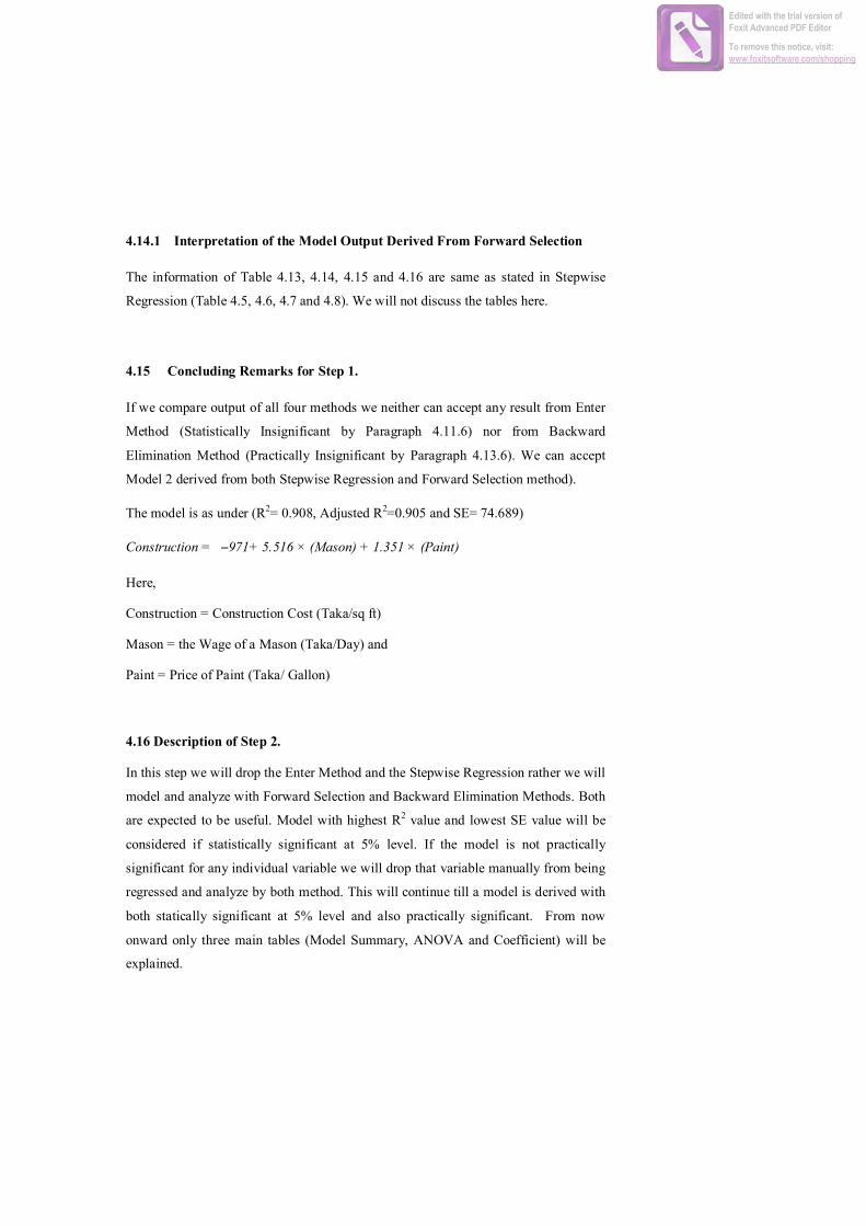


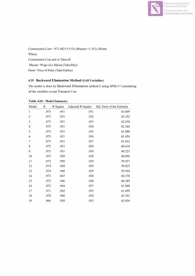


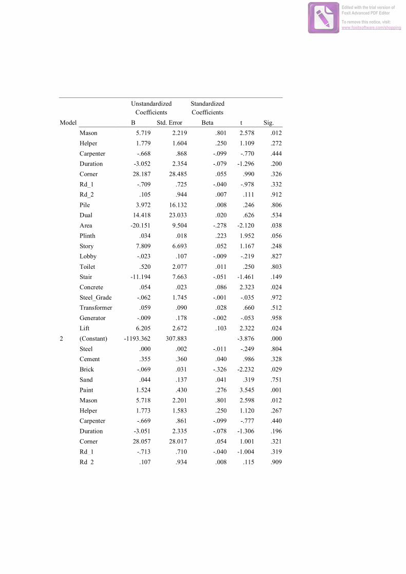


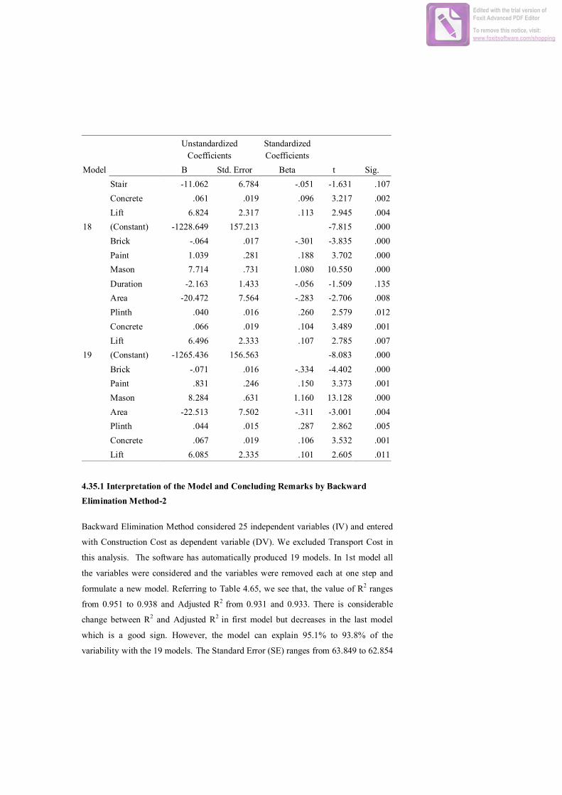


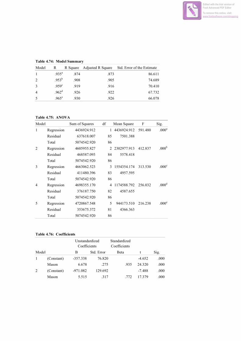


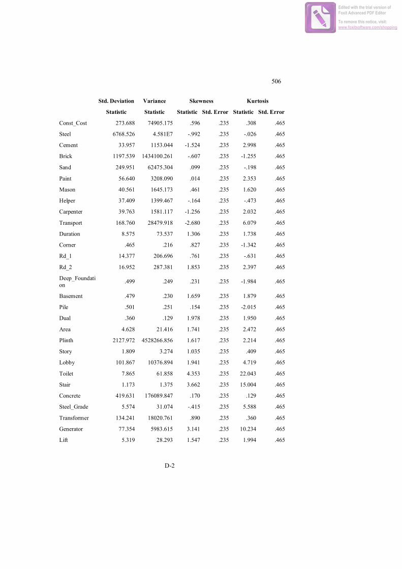


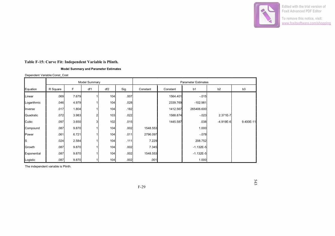


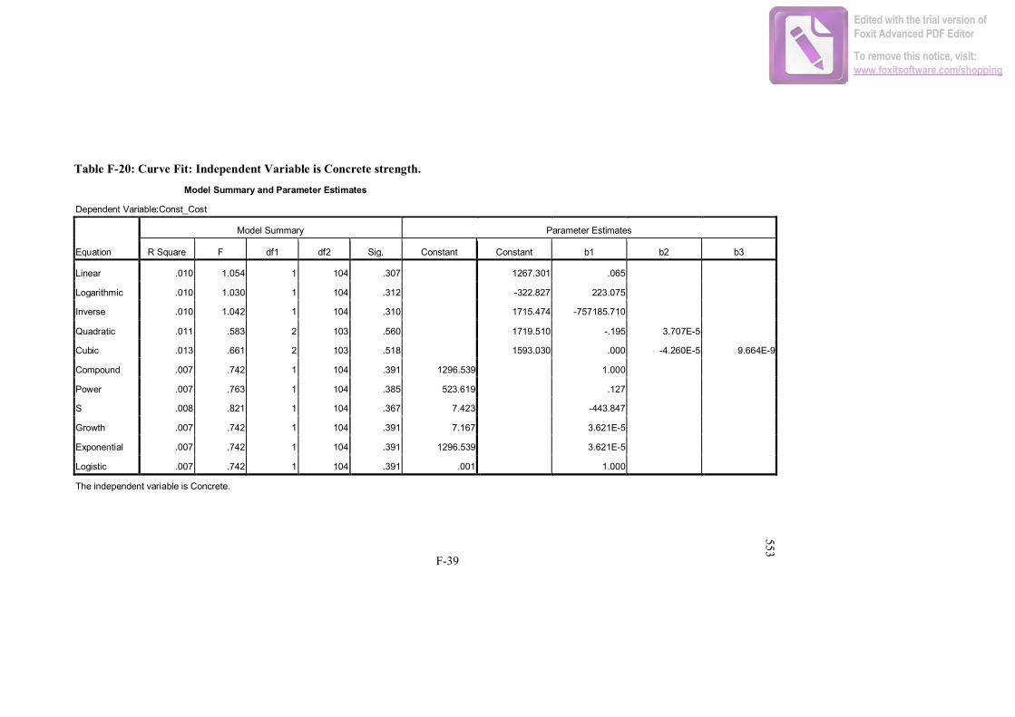


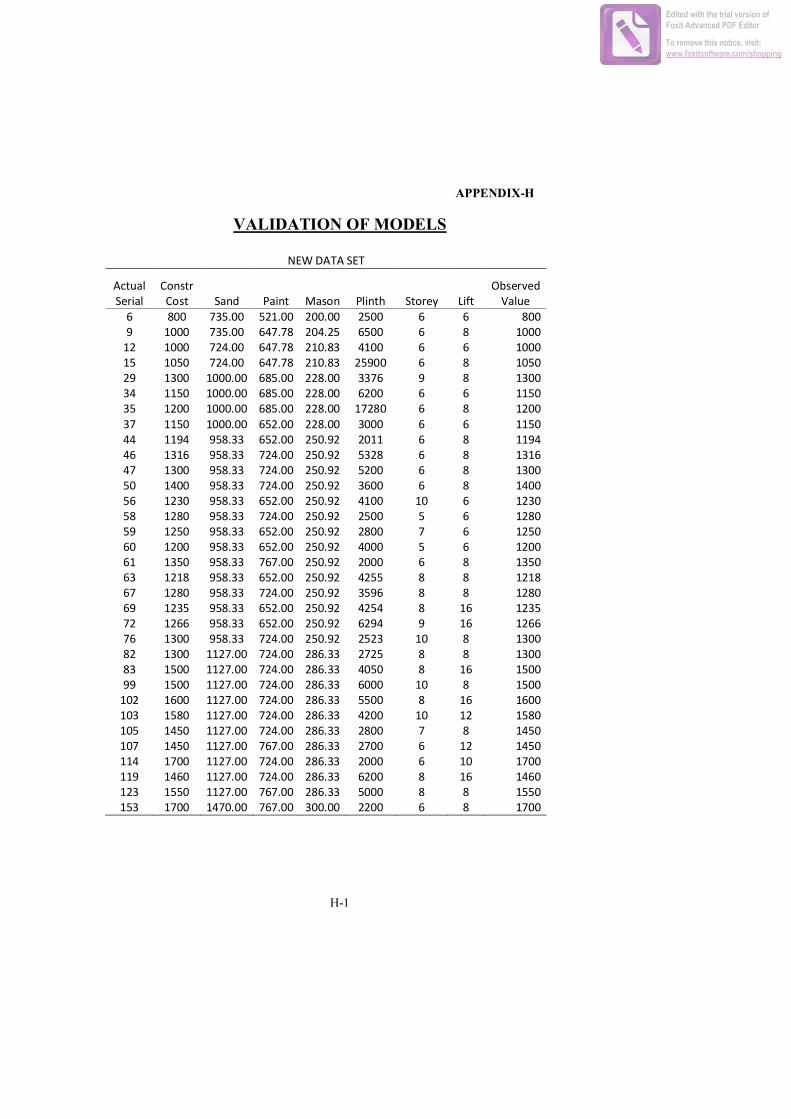


![Cost Function[1]](https://static.documents.pub/doc/80x56/577cc6bc1a28aba7119f0266/cost-function1.jpg)


