AUThoR Michael V. Bartolazo Mr. Bartolazo is Bank officer IV at the International operations Department of the BSP. he holds master degrees in Globalization and Development (with Distinction) from the Institute of Development Policy and Management from the University of Antwerp, Belgium in 2008, and Public Management from the UP Open University in 2003. He obtained his Bachelor’s degree in Statistics from the University of the Philippines in 1996. He has working experience on economic and financial surveillance, system of national accounts compilation, and econometric modelling. Developing a Philippine Composite Capital Flow Indicator (CCF)
Transcript
AUThoR
Michael V. Bartolazo
Mr. Bartolazo is Bank officer IV at the International operations Department of the BSP. he holds master degrees in Globalization and Development (with Distinction) from the Institute of Development Policy and Management from the University of Antwerp, Belgium in 2008, and Public Management from the UP Open University in 2003. He obtained his Bachelor’s degree in Statistics from the University of the Philippines in 1996. He has working experience on economic and financial surveillance, system of national accounts compilation, and econometric modelling.
Developing a Philippine CompositeCapital Flow Indicator (CCF)
A. Introduction
For the past decades, emerging market economies (EMEs) attracted
foreign private finance flows in addition to official development loans and
grants to support economic development. Increased globalization and
capital account liberalization has facilitated cross-border movements of
private capital which in turn has become an important feature of the global
economy. Cross-border flow of capital, in principle, has benefits for the
capital-importing and capital-exporting countries. However, capital flow
volatilities (e.g., surges and sudden stops) may result in macroeconomic
and financial stability issues. Capital surges, for instance, can overwhelm
domestic financial markets and strain the capacity of macroeconomic
policies. Moreover, such surges could lead to asset price bubbles, exchange
rate appreciation, and disruptions in monetary policy transmission, among
other effects (IMF, 2012).
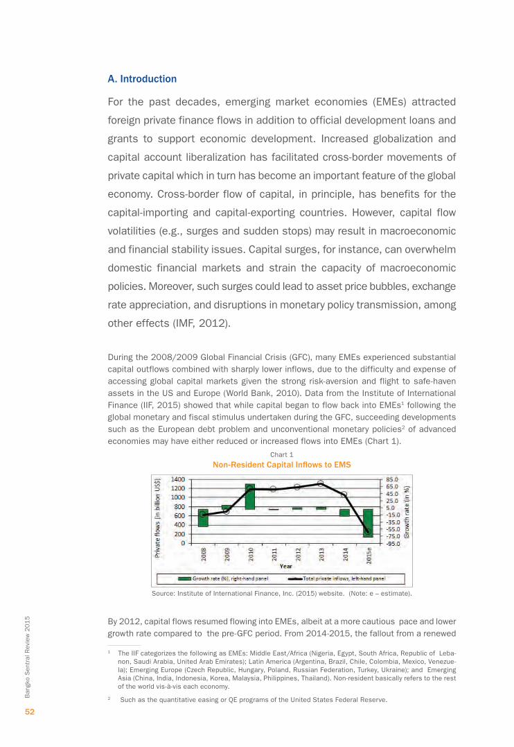
During the 2008/2009 Global Financial Crisis (GFC), many EMEs experienced substantial capital outflows combined with sharply lower inflows, due to the difficulty and expense of accessing global capital markets given the strong risk-aversion and flight to safe-haven assets in the US and Europe (World Bank, 2010). Data from the Institute of International Finance (IIF, 2015) showed that while capital began to flow back into EMEs1 following the global monetary and fiscal stimulus undertaken during the GFC, succeeding developments such as the European debt problem and unconventional monetary policies2 of advanced economies may have either reduced or increased flows into EMEs (Chart 1).
Chart 1
Non-Resident Capital Inflows to EMS
Source: Institute of International Finance, Inc. (2015) website. (note: e – estimate).
By 2012, capital flows resumed flowing into EMEs, albeit at a more cautious pace and lower growth rate compared to the pre-GFC period. From 2014-2015, the fallout from a renewed
1 The IIF categorizes the following as EMEs: Middle East/Africa (nigeria, Egypt, South Africa, Republic of Leba-non, Saudi Arabia, United Arab Emirates); Latin America (Argentina, Brazil, Chile, Colombia, Mexico, Venezue-la); Emerging Europe (Czech Republic, hungary, Poland, Russian Federation, Turkey, Ukraine); and Emerging Asia (China, India, Indonesia, Korea, Malaysia, Philippines, Thailand). non-resident basically refers to the rest of the world vis-à-vis each economy.
2 Such as the quantitative easing or QE programs of the United States Federal Reserve.
52
Ban
gko
Sen
tral
Rev
iew
2015
turmoil in the Euro area, expected policy normalization in the US, and volatilities in major EMEs such as China, may have kept back private flows. A similar trend in the growth rate is observed when IMF data on major items (liabilities side) from the Balance of Payments (BOP)3 of emerging economies is used (Table 1).
Table 1
BOP Financial Account (Liabilities side) of Emerging and Developing Economies, 2008-2015(in billion US$)
Source: (International Monetary Fund, 2016) – Balance of Payments aggregate data. n.a. – not available.
The Bank for International Settlements (BIS) argues that capital flows into EMEs tend to rise when financing conditions in investor countries ease and may move inversely with the business cycles in industrial countries (BIS, 2009). Moreover, ample global liquidity brought about by the low global interest environment and strong money supply growth in advanced economies are often cited as important factors that have “pushed” capital into EMEs (BIS, 2009).
In the Philippines, equity and debt flows from the BOP financial account in recent years showed that capital flows are marked by volatile inward portfolio investments and by more stable inward direct investment that continue to rise even after the GFC (Table 2).
Source: (Bangko Sentral ng Pilipinas, 2016) – Balance of Payments BPM6 Format, new Concept
Moral (2011) notes that a menu of options is available to the BSP to address the impact of capital flow surges. These include regulatory reforms and monetary policy approaches such as assessing and monitoring of Fx inflows; exchange rate flexibility; accumulation of reserves; macroprudential tools; enhanced monitoring and analysis of external debt; liquidity management; Fx regulatory reforms; capital market deepening; prepayment of foreign borrowings; monetary policy calibrations; and a balanced monetary-fiscal policy.
Several studies discussed the determinants of capital flows, their risks and effects on economic growth and the appropriate policy responses. Prior to the GFC, Lamberte (1995) found external factors such as search for better returns, portfolio diversification in advanced economies and internal factors to the Philippines such as credibility in instituting economic reforms and interest rate differentials (domestic and foreign), as factors attracting foreign investments. Tetangco (2005) observed that country-specific or pull factors of flows
3 The BOP and international investment position manual (IMF, 2009) defines the following components: a) direct investment pertains to cross-border investment associated with a resident in one economy having control or a significant degree of influence on the management of an enterprise that is resident in another economy; b) financial derivative contract is a financial instrument linked to another specific financial instrument or indica-tor or commodity and through which specific financial risks [e.g., interest rate, foreign exchange (Fx), equity, commodity price, credit risks, etc.] can be traded in their own right in financial markets; c) portfolio investment is crossborder transactions and positions involving debt or equity securities other than those included in di-rect investment or reserve assets; and d) other investment is a residual category that includes positions and transactions other than those included in a) to c) above and reserve assets.
53
Bangko S
entral Review
2015
include economic liberalization policies; improved macroeconomic fundamentals; increased investment opportunities and institutional reforms in some developing countries. Meanwhile, push factors of flows include structural and cyclical conditions in creditor countries which affect the timing and magnitude of flows.
Guinigundo (2014) studied the role played by global factors in the post-GFC period in affecting domestic monetary policy outturns. He found that for the Philippines, capital flow level and volatility have increased significantly since the GFC, and that the exchange rate, global financial risk-taking and inflation expectations were the main channels of international monetary policy transmission.4 Other researchers discussed welfare and inequality impacts of the different types of capital flows.5
For decades, the Philippines has undergone trade liberalization, deregulation, regulatory reforms and capital account liberalization. These reforms have in turn created a conducive environment for capital to flow into the economy.
This article proposes a way to track inward capital flows into the Philippines by constructing a quarterly composite index using a data reduction statistical procedure (i.e., PCA). Variables used were chosen based on their relative effect on inward “capital flows” into an open economy such as the Philippines. Five (5) variables were selected based on the availability of data (including higher frequency data); quick processing and manageability. The correlation of the constructed composite index and Philippine data on IIP (liabilities) was computed and was also compared. The PCA method was chosen over other methods like multiple regression because it allows for the condensation of the information contained in the five (5) original variables with minimal loss of information, and to draw conclusions from them rather than individually describing the trends of the different types of capital flows. An advantage of the PCA is that it can be performed, with caveats, even if the data for the month or quarter is not yet complete. Averages of past values or forecasts can be used so that the movement of “capital flows” can be anticipated in the immediately succeeding period while awaiting the official data releases from the BOP or IIP.
The focus in this study is mainly on gross capital inflows because of their potential implications to financial stability particularly during episodes of sudden reversals. net capital inflows may be more associated with the financing the current account. Forbes and Warnock (2011) developed a methodology, that used more detailed data on inflows and outflows by domestic and foreign investors to analyze extreme movements in capital flows.6
The construction of the composite indicator or index to analyze extreme movements in capital flows is a first in the Philippines. It is intended to serve as an additional analytical tool to aid our policymakers in formulating regulations on capital inflows. The article is organized as follows: Section B discusses the basis for the variables used in the study through a survey of related literature and the data processing steps; Section C tackles the methodology (i.e., PCA) used; Section D presents the PCA results and diagnostics, robustness checks; and Section E concludes.
4 In examining the impact of increasing financial intermediation in the Philippines on monetary policy transmission amidst surges in capital flows in the GFC aftermath, Guinigundo (2015), among other findings, maintained that the formulation of monetary policy and macroprudential policy needs to consider carefully the linkage with financial system and other financial shocks that arise internally and externally to the country.
5 Bartolazo (2008) found evidence that inward foreign direct investments have impact on manufacturing sector wage inequalities in a regional economic block.
6 The methodology of Forbes and Warnock (2011) yielded substantially different definitions of periods of capital flow waves, taking into account the foreign and domestic investors’ decision to increase or decrease their capital flows domestically and abroad, respectively.
54
Ban
gko
Sen
tral
Rev
iew
2015
B. Survey of related literatureThe choice of variables to be used in constructing the composite capital flow (CCF) is based on:
1. Supporting literature and previous empirical works that conform to economic theory, statistical significance and/or practical significance, wherein these variables measure aspects of the phenomenon of interest, i.e., “capital flows” (See details in section C).
2. Availability of timely, accurate and accessible data representing the chosen variables, as obtained from reputable organizations’ websites, Bloomberg L.P. Professional terminal, BSP website, and other sources, to ensure that other researchers can replicate this study.7
C. MethodologyC.1. Variables Used
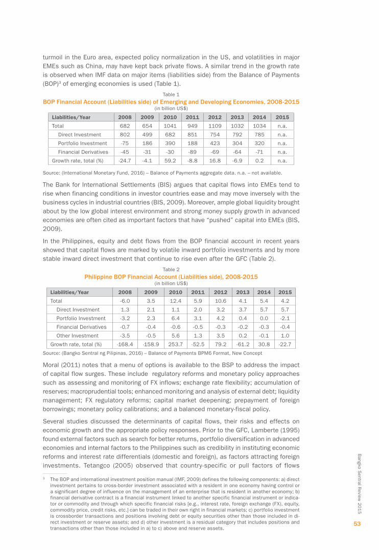
Table 3 summarizes the variables in this study:
Table 3
Indicators and variables usedIndicator Variable
namePeriod Definition Frequency Source of Data
a. Bonds BonDS Q4 2007 to Q2 2015
US Government Generic Treasury 10-year yield, in %
Daily (averaged into quarterly)
Bloomberg L.P. Professional terminal (2015)
b. Credit default swaps (CDS)
CDS Q4 2007 to Q2 2015
Philippine CDS, sovereign, 5-year, in basis points
Daily (averaged into quarterly)
Bloomberg L.P. Professional terminal (2015)
c. Gross international reserves (GIR) import cover
GIRIMP Q4 2007 to Q2 2015
Philippine GIR cover, in months of imports
Monthly (averaged into quarterly)
BSP website
d. Gross domestic product (GDP)
GDP Q4 2007 to Q2 2015
Philippine GDP real growth, in %
Quarterly BSP website
e. Business expectations survey
BConF Q4 2007 to Q2 2015
BSP Business Expectations Survey, of current quarter, index
Quarterly BSP website
f. International investment position (IIP)
not used in models; used only in chart for comparison
Q4 2007 to Q2 2015 (note: 2012 and earlier data are the author’s quarterly mputations)
Philippine IIP (liabilities side), in million US$
Quarterly BSP website
C.1.a. Bonds
The relatively low yield environment in advanced economies such as the US, euro area and Japan, where most of the capital flowing to the Philippines comes from, is a major “push” factor for capital. Byrne and Fiess (2011) found that the determinants of global capital flows include real long-run US interest rates both for aggregate flows and for disaggregate (bank and equity) flows.
7 The five (5) variables used in this study were aggregated into quarterly data. There may be long lags for some variables before becoming available publicly, especially that of GDP and GIR. In cases where quarterly data is not yet available, the author averaged the past three (3) quarters. For data with monthly frequency, monthly averages were also used to obtain a quarterly data.
55
Bangko S
entral Review
2015
C.1.b. CDS
During credit events such as a credit default or credit rating downgrades, CDS is usually used by investors for speculation, hedging or arbitrage. The study of Das, et. al. (2010) looked into the role of sovereign risk for private sector access to international capital markets a group of 31 emerging economies. They found that an increase in sovereign risk can have strong negative effects on corporate credit and equity volumes. Studying changes in US and European policy uncertainty and aggregate fund-level portfolio inflows across a global sample of EMEs including the Philippines, Gauvin et. al. (2014) used CDS spreads as proxy variable for the level of country-specific sovereign risk to determine the magnitude of policy uncertainty spillovers via equity flows.8
C.1.b. GIR import cover
The Philippines is a net importer of goods including petroleum and capital goods, among others. The GIR import cover is reflective of the availability Fx reserves as an external buffer. Currently, the country’s GIR is above international standards in terms of months’ of imports of goods, payments of services and income. The GIR should also be able to adequately cover the country’s short-term external debts, these being more transitory in nature and having lesser risk-sharing.9 Moreover, higgins and Klitgaard (2004) pointed out that central banks also accumulate reserves to “lean against the wind” when private capital inflows or outflows threaten to introduce disorderly movements (e.g., excessive appreciation or depreciation) in the domestic currency by selling (or buying) domestic assets and buying (or selling) foreign currency reserves.
C.1.d. GDP
Arguably, GDP as a measure of market size may be an all-encompassing variable, but several studies mentioned economic growth or its potential as a crucial consideration for foreign investors. GDP is also a commonly used indicator with other important variables, e.g., per capita income, debt service burden, external debt, international reserves and others. On the production side approach (by industry), GDP is the summation of Gross Value Added of all industries (economic activities) in the country, while GDP on the expenditure approach is the sum of the final uses of goods and services in the economy, valued at purchaser’s prices (BSP, 2014a). The BIS (2009) stated that a major element that pulls international capital to EMEs is the higher expected risk-adjusted returns due to better growth performance and a stable macroeconomic outlook, i.e., net private capital flows to EMEs tend to pick up whenever their economic growth surpasses that of the advanced economies.10
C.1.e. Business confidence
While global risk aversion plays a role in capital movements, sentiment towards an EME’s market may also be a consideration of investors, in terms of expectations, confidence and perceptions surveys (e.g., on corruption, ease of doing business, competitiveness, etc.). The BSP (2014b) said that its Business Expectations Survey dataset results provide advance information on the current and next periods’ economic and business conditions and other
8 Gauvin, et. al. (2014) argued that increased policy uncertainty (e.g., in EU) pushes portfolio equity into EMEs even if global risk is high, but only into countries with low sovereign default risk.
9 According to the BSP (n.d.), its International Reserves and Foreign Currency Liquidity data conforms to inter-nationally-accepted standards and guidelines specified in the IMF’s BOP Manual 6th Edition (BPM6) and the IMF’s operational Guidelines on International Reserves and Foreign Currency Liquidity.
10 Similarly, IMF (2011) identifies higher EME growth potential as a “pull” factor for foreign capital.56
Ban
gko
Sen
tral
Rev
iew
2015
indicators of aggregate demand that can be valuable in the formulation of monetary policy.11 The comprehensive list of respondents consisting of 1525 companies from 17 regions nationwide that were selected from the 2010 Securities and Exchange Commission’s Top 7,000 Corporations and 2012 Business world’s Top 1,000 Corporations (BSP, 2014b).
C.1.f. Philippine IIP
The BSP’s Philippine IIP data is available annually and on a quarterly basis starting in 2013, (BSP, 2015). The author computed for a quarterly IIP data series for 2012 and the earlier years (Table 4) using the annual IIP data (which are stock variables), by utilizing the items in the quarterly BOP data (which are flows variables) on: i) direct investment, ii) portfolio investment, iii) financial derivatives, and iv) other investment.
Table 4
Quarterly Philippines International Investment Position (IIP), liabilities (BPM6)as of periods indicated
Source of basic data: BSP website (note: author computed for the quarterly data from 2012 and earlier using quarterly BOP items)
note: Details may not add up to totals due to rounding.
C.2. Method Used
C.2.a. The PCA method
The five (5) variables attempted to explain aspects of movements in capital flows, using PCA as a data reduction technique. PCA allows the reduction of the complexity of high-dimensional data and approximate high-dimensional data into fewer dimensions (SAS, 2014). Each dimension is called a principal component (PC) and represents a linear combination of the original variables, where the first PC accounts for as much variation in the data as possible. Subsequent PCs account for the remaining variation and is orthogonal to all of
11 Examples of such indicators are the levels of production and economic activity and other factors that could influence the movement of key economic variables such as GDP, interest rates, peso/Fx rate and inflation rate (BSP, 2014b).
57
Bangko S
entral Review
2015
the previous PCs. For PCA to be meaningful, the first PC should be somewhat correlated with many of the variables, while succeeding components should be correlated with some of the variables that had low correlations with the first, and so on (SAS, 2014).
The extracted components, i.e., the eigenvalues which correspond to the PCs and which represent a partitioning of the total variation in the sample and because correlations are used, the sum of all the eigenvalues is equal to the number of variables (SAS, 2014). Additionally, the extracted eigenvectors of the correlation matrix are PC vectors, where each PC is a linear combination of the total number of variables (SAS, 2014).
Some studies by monetary authorities utilized PCA in the construction of a composite index, such as the St. Louis Fed’s Financial Stress Index (Federal Reserve Bank of St. Louis, 2010) which used 18 variables to capture aspects of a phenomenon they are measuring that is assumed to be the main factor in the variables’ co-movement.
C.2.b. PCA diagnostics
Before PCA was performed, a number of diagnostic checks were made to the variables and data used. The following assumptions suggested in Laerd Statistics (n.d.) were checked:
1. The multiple variables are measured at the continuous level (i.e., ratio and interval scales). The five (5) variables used in this study are all continuous ones.
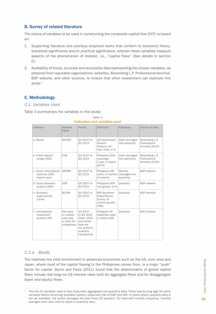
2. The variables should have linear relationships. Rudimentary scatterplots suggest that generally the variables have some linear relationships to each other (Chart 2).
Chart 2
58
Ban
gko
Sen
tral
Rev
iew
2015
3. Sampling adequacy. For PCA to be more reliable, large sample is desired. Several rules of thumbs on minimum samples were put forward such as 150 cases or five (5) to 10 per variable, which this study is compliant with.12
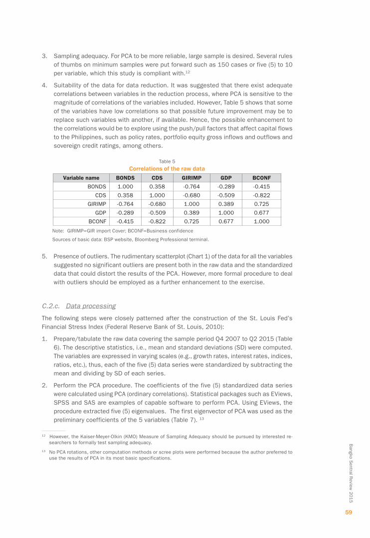
4. Suitability of the data for data reduction. It was suggested that there exist adequate correlations between variables in the reduction process, where PCA is sensitive to the magnitude of correlations of the variables included. However, Table 5 shows that some of the variables have low correlations so that possible future improvement may be to replace such variables with another, if available. Hence, the possible enhancement to the correlations would be to explore using the push/pull factors that affect capital flows to the Philippines, such as policy rates, portfolio equity gross inflows and outflows and sovereign credit ratings, among others.
Table 5
Correlations of the raw dataVariablename BONDS CDS GIRIMP GDP BCONF
Sources of basic data: BSP website, Bloomberg Professional terminal. 5. Presence of outliers. The rudimentary scatterplot (Chart 1) of the data for all the variables
suggested no significant outliers are present both in the raw data and the standardized data that could distort the results of the PCA. however, more formal procedure to deal with outliers should be employed as a further enhancement to the exercise.
C.2.c. Data processing
The following steps were closely patterned after the construction of the St. Louis Fed’s Financial Stress Index (Federal Reserve Bank of St. Louis, 2010):
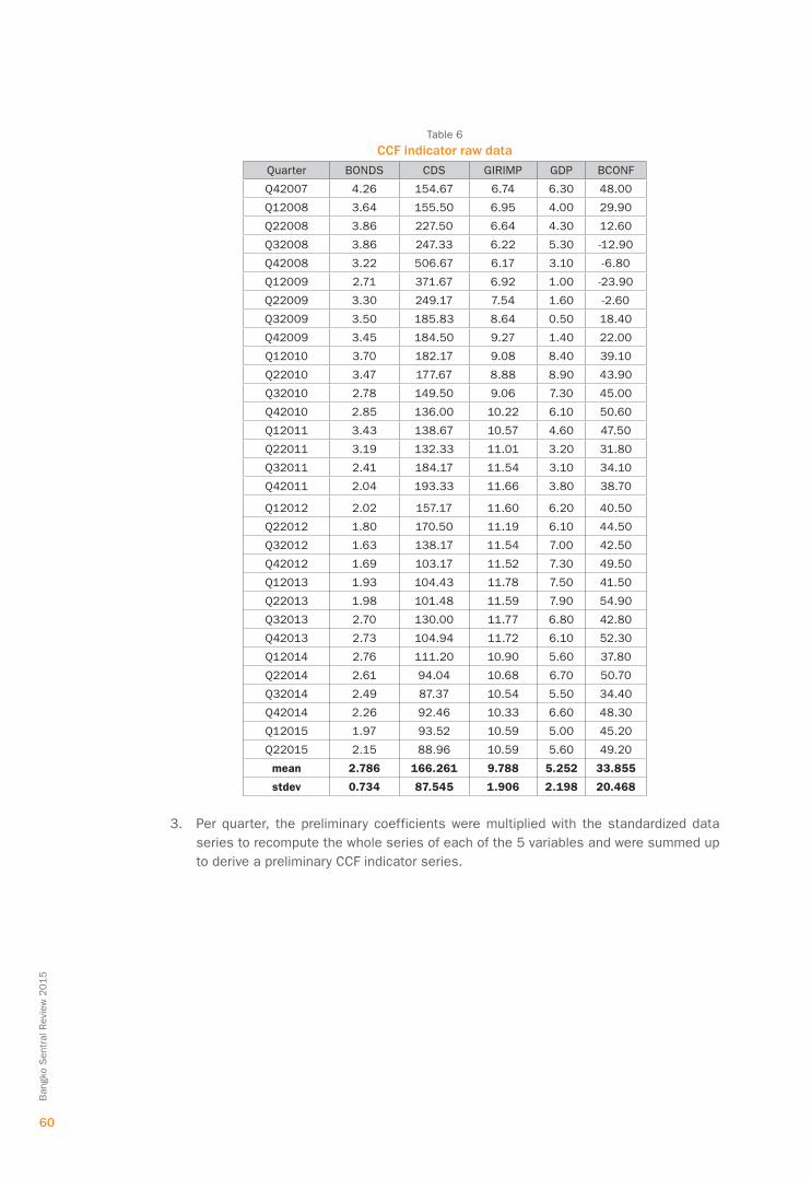
1. Prepare/tabulate the raw data covering the sample period Q4 2007 to Q2 2015 (Table 6). The descriptive statistics, i.e., mean and standard deviations (SD) were computed. The variables are expressed in varying scales (e.g., growth rates, interest rates, indices, ratios, etc.), thus, each of the five (5) data series were standardized by subtracting the mean and dividing by SD of each series.
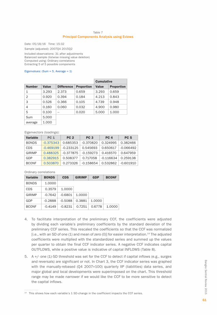
2. Perform the PCA procedure. The coefficients of the five (5) standardized data series were calculated using PCA (ordinary correlations). Statistical packages such as EViews, SPSS and SAS are examples of capable software to perform PCA. Using EViews, the procedure extracted five (5) eigenvalues. The first eigenvector of PCA was used as the preliminary coefficients of the 5 variables (Table 7). 13
12 however, the Kaiser-Meyer-olkin (KMo) Measure of Sampling Adequacy should be pursued by interested re-searchers to formally test sampling adequacy.
13 no PCA rotations, other computation methods or scree plots were performed because the author preferred to use the results of PCA in its most basic specifications.
59
Bangko S
entral Review
2015
Table 6
CCF indicator raw dataQuarter BonDS CDS GIRIMP GDP BConF
Q42007 4.26 154.67 6.74 6.30 48.00
Q12008 3.64 155.50 6.95 4.00 29.90
Q22008 3.86 227.50 6.64 4.30 12.60
Q32008 3.86 247.33 6.22 5.30 -12.90
Q42008 3.22 506.67 6.17 3.10 -6.80
Q12009 2.71 371.67 6.92 1.00 -23.90
Q22009 3.30 249.17 7.54 1.60 -2.60
Q32009 3.50 185.83 8.64 0.50 18.40
Q42009 3.45 184.50 9.27 1.40 22.00
Q12010 3.70 182.17 9.08 8.40 39.10
Q22010 3.47 177.67 8.88 8.90 43.90
Q32010 2.78 149.50 9.06 7.30 45.00
Q42010 2.85 136.00 10.22 6.10 50.60
Q12011 3.43 138.67 10.57 4.60 47.50
Q22011 3.19 132.33 11.01 3.20 31.80
Q32011 2.41 184.17 11.54 3.10 34.10
Q42011 2.04 193.33 11.66 3.80 38.70
Q12012 2.02 157.17 11.60 6.20 40.50
Q22012 1.80 170.50 11.19 6.10 44.50
Q32012 1.63 138.17 11.54 7.00 42.50
Q42012 1.69 103.17 11.52 7.30 49.50
Q12013 1.93 104.43 11.78 7.50 41.50
Q22013 1.98 101.48 11.59 7.90 54.90
Q32013 2.70 130.00 11.77 6.80 42.80
Q42013 2.73 104.94 11.72 6.10 52.30
Q12014 2.76 111.20 10.90 5.60 37.80
Q22014 2.61 94.04 10.68 6.70 50.70
Q32014 2.49 87.37 10.54 5.50 34.40
Q42014 2.26 92.46 10.33 6.60 48.30
Q12015 1.97 93.52 10.59 5.00 45.20
Q22015 2.15 88.96 10.59 5.60 49.20
mean 2.786 166.261 9.788 5.252 33.855
stdev 0.734 87.545 1.906 2.198 20.468
3. Per quarter, the preliminary coefficients were multiplied with the standardized data series to recompute the whole series of each of the 5 variables and were summed up to derive a preliminary CCF indicator series.
60
Ban
gko
Sen
tral
Rev
iew
2015
Table 7
Principal Components Analysis using Eviews
Date: 05/18/16 Time: 15:32
Sample (adjusted): 2007Q4 2015Q2
Included observations: 31 after adjustmentsBalanced sample (listwise missing value deletion)Computed using: Ordinary correlationsExtracting 5 of 5 possible components Eigenvalues: (Sum = 5, Average = 1)
Cumulative
Number Value Difference Proportion Value Proportion
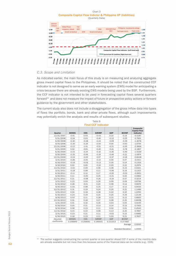
4. To facilitate interpretation of the preliminary CCF, the coefficients were adjusted by dividing each variable’s preliminary coefficients by the standard deviation of the preliminary CCF series. This rescaled the coefficients so that the CCF was normalized [i.e., with an SD of one (1) and mean of zero (0)] for easier interpretation.14 The adjusted coefficients were multiplied with the standardized series and summed up the values per quarter to obtain the final CCF indicator series. A negative CCF indicates capital oUTFLowS, while a positive value is indicative of capital InFLowS (Table 8).
5. A +/- one (1)-SD threshold was set for the CCF to detect if capital inflows (e.g., surges and reversals) are significant or not. In Chart 3, the CCF indicator series was graphed with the manually-rebased (Q4 2007=100) quarterly IIP (liabilities) data series, and major global and local developments were superimposed on the chart. This threshold range may be made narrower if we would like the CCF to be more sensitive to detect the capital inflows.
14 This shows how each variable’s 1 SD-change in the coefficient impacts the CCF series.
61
Bangko S
entral Review
2015
Chart 3
Composite Capital Flow Indictor & Philippine IIP (liabilities)(Quarterly Data)
0.70
0.80
0.90
1.00
1.10
1.20
1.30
1.40
1.50
1.60
-2.50
-2.00
-1.50
-1.00
-0.50
0.00
0.50
1.00
1.50
Composite Capital Flow Indicator (Left-hand axis)
Quarterlized IIP (Liabilities) (Right-hand axis)
Lehman collapse
Fed QE1
Greek 1st bailout
Fed QE2
EFSF
Global fiscal, monetary stimuli
Greek 2nd bailoutESM ECB OMT/Fed
QE3
Philippine investments ratings
Fed taper starts Taper ends
C.3. Scope and Limitation
As indicated earlier, the main focus of this study is on measuring and analyzing aggregate gross inward capital flows to the Philippines. It should be noted that the constructed CCF indicator is not designed to serve as an early warning system (EWS) model for anticipating a crisis because there are already existing EWS models being used by the BSP. Furthermore, the CCF indicator is not intended to be used in forecasting capital flows several quarters forward15 and does not measure the impact of future or prospective policy actions or forward guidance by the government and other stakeholders.
The current study also does not include a disaggregation of the gross inflow data into types of flows like portfolio, bonds, bank and other private flows, although such improvements may potentially enrich the analysis and results of subsequent studies.
Table 8
Final CCF Indicator
Quarter BONDS CDS GIRIMP GDP BCONF
Composite Capital Flow
Indicator
12/31/2007 -0.41 0.03 -0.43 0.10 0.19 -0.5187
3/31/2008 -0.24 0.03 -0.40 -0.12 -0.05 -0.7831
6/30/2008 -0.30 -0.18 -0.44 -0.09 -0.29 -1.3078
9/30/2008 -0.30 -0.24 -0.50 0.00 -0.63 -1.6744
12/31/2008 -0.12 -1.01 -0.51 -0.21 -0.55 -2.3956
3/31/2009 0.02 -0.61 -0.40 -0.41 -0.78 -2.1807
6/30/2009 -0.15 -0.24 -0.32 -0.35 -0.49 -1.5539
9/30/2009 -0.20 -0.06 -0.16 -0.46 -0.21 -1.0874
12/31/2009 -0.19 -0.05 -0.07 -0.37 -0.16 -0.8438
3/31/2010 -0.26 -0.05 -0.10 0.30 0.07 -0.0311
6/30/2010 -0.19 -0.03 -0.13 0.35 0.14 0.1316
9/30/2010 0.00 0.05 -0.10 0.20 0.15 0.2974
12/31/2010 -0.02 0.09 0.06 0.08 0.23 0.4421
3/31/2011 -0.18 0.08 0.11 -0.06 0.19 0.1310
6/30/2011 -0.11 0.10 0.17 -0.20 -0.03 -0.0651
9/30/2011 0.11 -0.05 0.25 -0.21 0.00 0.0962
12/31/2011 0.21 -0.08 0.26 -0.14 0.07 0.3214
3/31/2012 0.22 0.03 0.26 0.09 0.09 0.6799
6/30/2012 0.28 -0.01 0.20 0.08 0.14 0.6876
9/30/2012 0.33 0.08 0.25 0.17 0.12 0.9420
12/31/2012 0.31 0.19 0.24 0.20 0.21 1.1489
3/31/2013 0.24 0.18 0.28 0.22 0.10 1.0250
6/30/2013 0.23 0.19 0.25 0.25 0.29 1.2139
9/30/2013 0.03 0.11 0.28 0.15 0.12 0.6820
12/31/2013 0.01 0.18 0.27 0.08 0.25 0.8008
3/31/2014 0.01 0.16 0.16 0.03 0.05 0.4155
6/30/2014 0.05 0.21 0.13 0.14 0.23 0.7563
9/30/2014 0.08 0.23 0.11 0.02 0.01 0.4543
12/31/2014 0.15 0.22 0.08 0.13 0.20 0.7667
3/31/2015 0.23 0.21 0.11 -0.02 0.15 0.6882
6/30/2015 0.18 0.23 0.11 0.03 0.21 0.7607
Adjusted coefficients
BonDS CDS GIRIMP GDP BConF
-0.206840 -0.258561 0.269101 0.211013 0.277667
Average
Standard Deviation
0.0000
1.0000
15 The author suggests constructing the current quarter or one-quarter ahead CCF if some of the monthly data are already available but not more than this because some of the financial data can be volatile (e.g., CDS).
62
Ban
gko
Sen
tral
Rev
iew
2015
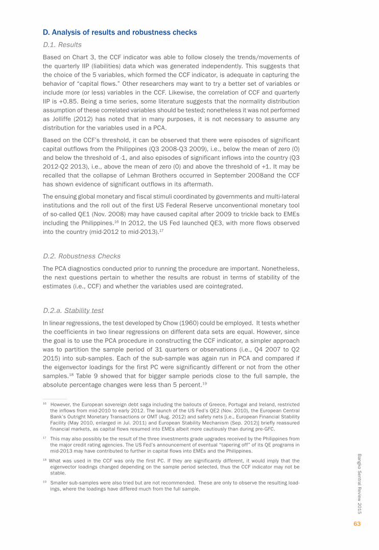
D. Analysis of results and robustness checksD.1. Results
Based on Chart 3, the CCF indicator was able to follow closely the trends/movements of the quarterly IIP (liabilities) data which was generated independently. This suggests that the choice of the 5 variables, which formed the CCF indicator, is adequate in capturing the behavior of “capital flows.” Other researchers may want to try a better set of variables or include more (or less) variables in the CCF. Likewise, the correlation of CCF and quarterly IIP is +0.85. Being a time series, some literature suggests that the normality distribution assumption of these correlated variables should be tested; nonetheless it was not performed as Jolliffe (2012) has noted that in many purposes, it is not necessary to assume any distribution for the variables used in a PCA.
Based on the CCF’s threshold, it can be observed that there were episodes of significant capital outflows from the Philippines (Q3 2008-Q3 2009), i.e., below the mean of zero (0) and below the threshold of -1, and also episodes of significant inflows into the country (Q3 2012-Q2 2013), i.e., above the mean of zero (0) and above the threshold of +1. It may be recalled that the collapse of Lehman Brothers occurred in September 2008and the CCF has shown evidence of significant outflows in its aftermath.
The ensuing global monetary and fiscal stimuli coordinated by governments and multi-lateral institutions and the roll out of the first US Federal Reserve unconventional monetary tool of so-called QE1 (nov. 2008) may have caused capital after 2009 to trickle back to EMEs including the Philippines.16 In 2012, the US Fed launched QE3, with more flows observed into the country (mid-2012 to mid-2013).17
D.2. Robustness Checks
The PCA diagnostics conducted prior to running the procedure are important. nonetheless, the next questions pertain to whether the results are robust in terms of stability of the estimates (i.e., CCF) and whether the variables used are cointegrated.
D.2.a. Stability test
In linear regressions, the test developed by Chow (1960) could be employed. It tests whether the coefficients in two linear regressions on different data sets are equal. However, since the goal is to use the PCA procedure in constructing the CCF indicator, a simpler approach was to partition the sample period of 31 quarters or observations (i.e., Q4 2007 to Q2 2015) into sub-samples. Each of the sub-sample was again run in PCA and compared if the eigenvector loadings for the first PC were significantly different or not from the other samples.18 Table 9 showed that for bigger sample periods close to the full sample, the absolute percentage changes were less than 5 percent.19
16 However, the European sovereign debt saga including the bailouts of Greece, Portugal and Ireland, restricted the inflows from mid-2010 to early 2012. The launch of the US Fed’s QE2 (nov. 2010), the European Central Bank’s outright Monetary Transactions or oMT (Aug. 2012) and safety nets [i.e., European Financial Stability Facility (May 2010, enlarged in Jul. 2011) and European Stability Mechanism (Sep. 2012)] briefly reassured financial markets, as capital flows resumed into EMEs albeit more cautiously than during pre-GFC.
17 This may also possibly be the result of the three investments grade upgrades received by the Philippines from the major credit rating agencies. The US Fed’s announcement of eventual “tapering off” of its QE programs in mid-2013 may have contributed to further in capital flows into EMEs and the Philippines.
18 What was used in the CCF was only the first PC. If they are significantly different, it would imply that the eigenvector loadings changed depending on the sample period selected, thus the CCF indicator may not be stable.
19 Smaller sub-samples were also tried but are not recommended. These are only to observe the resulting load-ings, where the loadings have differed much from the full sample.
63
Bangko S
entral Review
2015
Table 9
Summary of PCA Runs in EViews on Sub-Samples (1st Principal components only)
Sample periodNo. of
observations1st Principal components
BONDS CDS GIRIMP GDP BCONFa. FULL sample (Q4 2007-Q2 2015)
PercentagechangefromFULLsampleSample period BONDS CDS GIRIMP GDP BCONF
a. FULL sample (Q4 2007-Q2 2015)
- - - - - - - - - -
b. SUB sample (Q4 2007-Q3 2014)
-3.1 -0.5 0.9 1.8 0.2
c. SUB sample (Q3 2008-Q2 2015)
-2.1 0.1 1.3 -1.7 0.8
d. SUB sample (Q4 2007-Q2 2011)
-114.7 15.6 -6.2 1.8 15.9
e. SUB sample (Q3 2011-Q2 2015)
-91.8 25.3 -145.3 42.4 10.0
D.2.a. Cointegration with selected indicators
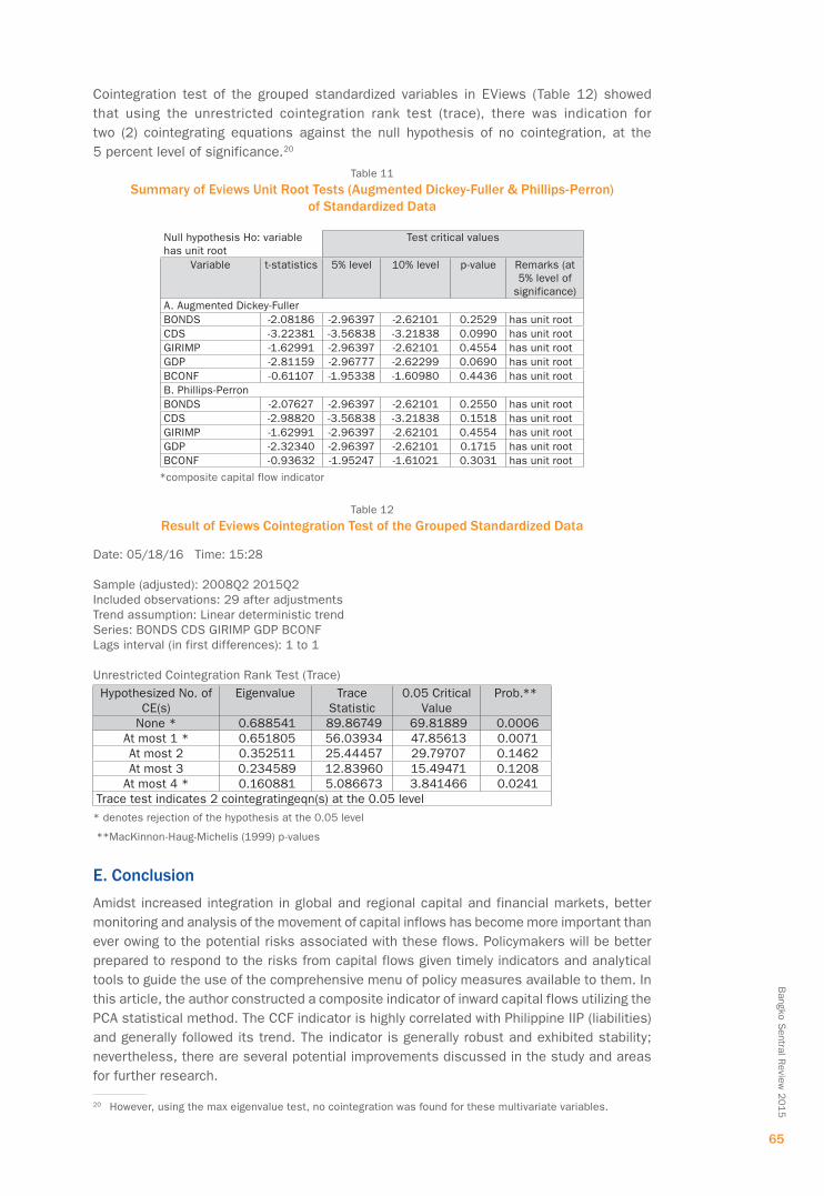
In a study, Bayangos (2000) mentioned that a non-stationary series exhibits some upward or downward trend over time (i.e., implying a non-constant variance) and that it does not tend to go back over time to its average value after a random disturbance and drifts away just like a random walk, an indication that it has a unit root. Unit root tests on both the raw and standardized data sets using the Augmented Dickey-Fuller (ADF) and Phillips-Perron (PP) test were performed to determine whether the time series data exhibited stationarity, i.e., a series has constant mean and variance over time. At the 5 percent level of significance, results summarized in Table 10 showed that all variables have unit root. Meanwhile, the unit root tests on the standardized variables (Table 11) showed that BonDS, GIRIMP, GDP and the CCF indicator have no unit roots using ADF, while only BonDS and GDP have no unit roots using PP.
Table 10
Summary of Eviews Unit Root Tests (Augmented Dickey-Fuller & Phillips-Perron) of Raw Data
significance)A. Augmented Dickey-FullerBonDS -2.08186 -2.96397 -2.62101 0.2529 has unit rootCDS -3.22381 -3.56838 -3.21838 0.0990 has unit rootGIRIMP -1.62991 -2.96397 -2.62101 0.4554 has unit rootGDP -2.81159 -2.96777 -2.62299 0.0690 has unit rootBConF -0.61107 -1.95338 -1.60980 0.4436 has unit rootB. Phillips-PerronBonDS -2.07627 -2.96397 -2.62101 0.2550 has unit rootCDS -2.98820 -3.56838 -3.21838 0.1518 has unit rootGIRIMP -1.62991 -2.96397 -2.62101 0.4554 has unit rootGDP -2.32340 -2.96397 -2.62101 0.1715 has unit rootBConF -0.93632 -1.95247 -1.61021 0.3031 has unit root
64
Ban
gko
Sen
tral
Rev
iew
2015
Cointegration test of the grouped standardized variables in EViews (Table 12) showed that using the unrestricted cointegration rank test (trace), there was indication for two (2) cointegrating equations against the null hypothesis of no cointegration, at the 5 percent level of significance.20
Table 11
Summary of Eviews Unit Root Tests (Augmented Dickey-Fuller & Phillips-Perron) of Standardized Data
significance)A. Augmented Dickey-FullerBonDS -2.08186 -2.96397 -2.62101 0.2529 has unit rootCDS -3.22381 -3.56838 -3.21838 0.0990 has unit rootGIRIMP -1.62991 -2.96397 -2.62101 0.4554 has unit rootGDP -2.81159 -2.96777 -2.62299 0.0690 has unit rootBConF -0.61107 -1.95338 -1.60980 0.4436 has unit rootB. Phillips-PerronBonDS -2.07627 -2.96397 -2.62101 0.2550 has unit rootCDS -2.98820 -3.56838 -3.21838 0.1518 has unit rootGIRIMP -1.62991 -2.96397 -2.62101 0.4554 has unit rootGDP -2.32340 -2.96397 -2.62101 0.1715 has unit rootBConF -0.93632 -1.95247 -1.61021 0.3031 has unit root
*composite capital flow indicator
Table 12
Result of Eviews Cointegration Test of the Grouped Standardized Data
Date: 05/18/16 Time: 15:28
Sample (adjusted): 2008Q2 2015Q2Included observations: 29 after adjustmentsTrend assumption: Linear deterministic trendSeries: BonDS CDS GIRIMP GDP BConFLags interval (in first differences): 1 to 1 Unrestricted Cointegration Rank Test (Trace)
hypothesized no. of CE(s)
Eigenvalue Trace Statistic
0.05 Critical Value
Prob.**
none * 0.688541 89.86749 69.81889 0.0006At most 1 * 0.651805 56.03934 47.85613 0.0071At most 2 0.352511 25.44457 29.79707 0.1462At most 3 0.234589 12.83960 15.49471 0.1208
At most 4 * 0.160881 5.086673 3.841466 0.0241Trace test indicates 2 cointegratingeqn(s) at the 0.05 level
* denotes rejection of the hypothesis at the 0.05 level
**MacKinnon-haug-Michelis (1999) p-values
E. Conclusion Amidst increased integration in global and regional capital and financial markets, better monitoring and analysis of the movement of capital inflows has become more important than ever owing to the potential risks associated with these flows. Policymakers will be better prepared to respond to the risks from capital flows given timely indicators and analytical tools to guide the use of the comprehensive menu of policy measures available to them. In this article, the author constructed a composite indicator of inward capital flows utilizing the PCA statistical method. The CCF indicator is highly correlated with Philippine IIP (liabilities) and generally followed its trend. The indicator is generally robust and exhibited stability; nevertheless, there are several potential improvements discussed in the study and areas for further research.
20 However, using the max eigenvalue test, no cointegration was found for these multivariate variables.
65
Bangko S
entral Review
2015
ReferencesBank for International Settlements (BIS) (2009). Capital flows and emerging market economies. Basel, Switzerland:
Committee on the Global Financial System.
Bangko Sentral ng Pilipinas (BSP) (n.d.). Metadata - international reserves and foreign currency liquidity. Retrieved from BSP website: http://www.bsp.gov.ph/statistics/ Metadata/International%20Reserves%20of%20the%20BSP_metadata.pdf
BSP (2014a). Metadata - national accounts. Retrieved from BSP website: http://www.bsp.gov.ph/statistics/Metadata/ national%20Accounts-metadata.pdf
BSP (2014b). Metadata – Business expectations survey. Retrieved from BSP website: http://www.bsp.gov.ph/statistics/Metadata/Business%20Expectations%20Survey metadata.pdf
BSP (2015). Economic and financial statistics - international investment position, BPM6 format [Data file]. Retrieved from BSP website: http://www.bsp.gov.ph/statistics/ excel/iip_bpm6.xls
BSP (2016). Economic and financial statistics - balance of payments, BPM6 format, new concept [Data file]. Retrieved from BSP website: http://www.bsp.gov.ph/ statistics/excel/bpm6.xls
Bartolazo, M. (2008). Effects of inward FDI on the Association of Southeast Asian nation’s manufacturing wage inequality (Unpublished master dissertation). Institute of Development Policy and Management, University of Antwerp, Belgium.
Bayangos, V. (2000). A real monetary conditions index for the Philippines: is it useful? Institute of Social Studies working Paper Series no. 309.
Bloomberg L.P. (2015). Various Bloomberg L.P. Professional terminal data, Q4 2007 to Q2 2015. Retrieved october 07, 2015 from Bloomberg database.
Byrne, J. P., & Fiess, n. (2011). International capital flows to emerging and developing countries: national and global determinants. University of Glasgow working Paper 01/10/2011.
Chow, G. (1960). Tests of equality between sets of coefficients in two linear regressions. Econometrica, 28(3), 591–605.
Das, U. S., Papaioannou, M., & Trebesch, C. (2010). Sovereign default risk and private sector access to capital in emerging markets. IMF working Paper no. wP/10/10.
Federal Reserve Bank of St. Louis (2010). Appendix. national Economic Trends, 1-2.
Forbes, K. J., & warnock, F. (2011, August). Capital flow waves: surges, stops, flight, and retrenchment. national Bureau of Economic Research (nBER) working Paper Series no. 17351.
Gauvin, L., McLoughlin, C., & Reinhardt, D. (2014, november 5). Policy uncertainty spillovers to emerging markets: evidence from capital flows. Retrieved from Vox CEPR’s Policy Portal website: http://www.voxeu.org/print/58206.
Guinigundo, D. (2014). what have emerging market central banks learned about the international transmission of monetary policy in recent years? The Philippine case. In BIS Papers, The transmission of unconventional monetary policy to the emerging markets, (pp. 265-283). Basel, Switzerland: Bank for International Settlements (BIS).
Guinigundo, D. (2015). Increased financial intermediation in the Philippines: some implications for monetary policy. In BIS Papers, what do new forms of finance mean for EM central banks? (pp. 293-311). Basel, Switzerland: BIS.
higgins, M., & Klitgaard, T. (2004). Reserve accumulation: implications for global capital flows and financial markets. Current Issues In Economics and Finance, 10(10), 1-8.
Institute of International Finance (IIF) (2015). Aggregate capital flows data [Data file]. Retrieved from IIF website: https://www.iif.com/system/files/annual_em_ capital_flows_ database.xls
International Monetary Fund (IMF) (2009). Balance of payments and international investment position manual. Washington, D.C.: IMF.
IMF (2011). Recent experiences in managing capital inflows—cross-cutting themes and possible policy framework. washington D.C., USA: Strategy, Policy, and Review Department.
IMF (2012). The liberalization and management of capital flows: an institutional view. washington D.C., USA: IMF Staff.
IMF (2016, January 11). world and regional tables: balance of payments by indicator (BPM6) [Data file]. Retrieved from IMF website: http://data.imf.org/ regular.aspx?key=60961513
Jolliffe, I. (2002). Principal component analysis, second edition. new york, ny: Springer-Verlag new york, Incorporated.
Laerd Statistics (n.d.). Principal Components Analysis (PCA) using SPSS Statistics. Retrieved from Laerd Statistics website: https://statistics.laerd.com/spss-tutorials/principal-components-analysis-pca-using-spss-statistics.php
Lamberte, M. (1995). Managing surges in capital inflows: the Philippine Case. Journal of Philippine Development, 22(1), 43-88.
Moral, G. (2011, March-April). Coping with surges in capital flows. BSP Economic newsletter, 11(02), 1-5.
SAS Institute Incorporated. (2014). SAS/IML® Studio 13.2: User’s Guide. Cary, nC: SAS Institute Inc.
Tetangco, A. (2005). The composition and management of capital flows in the Philippines. In BIS Papers, Globalisation and monetary policy in emerging markets (pp. 242-259). Basel, Switzerland: BIS.
world Bank (2010). how to manage capital flows in a globalized world? Issues and policy challenges: global development debate on how to manage capital flows. Retrieved from world Bank website: http://developmentdebates.ning.com/page/global-development-debate-on?xg_source=activity