Developing a Wisconsin Wetland Change Analysis & Building Compliance Monitoring Efforts Understanding Wetland Changes in West-Central and North-Western Wisconsin Final Report to the USEAPA, Region V EPA Wetland Program Development Grant No. 00E00756 September 2015 Prepared by: Wisconsin Department of Natural Resources Bureau of Watershed Management 101 S. Webster St., Madison, WI 53707 Authors: Sally Gallagher Jarosz and Daniel Haug Editors: Lois Simon and Cami Peterson
Transcript
Developing a Wisconsin Wetland Change Analysis & Building Compliance Monitoring Efforts
Understanding Wetland Changes in West-Central and North-Western Wisconsin
Final Report to the USEAPA, Region V EPA Wetland Program Development Grant No. 00E00756
September 2015
Prepared by: Wisconsin Department of Natural Resources Bureau of Watershed Management 101 S. Webster St., Madison, WI 53707
Authors: Sally Gallagher Jarosz and Daniel Haug
Editors: Lois Simon and Cami Peterson
Table of Contents:
1) Introduction 2) Project Goals 3) Analysis of Wetland Changes in Study Area 1: Wood, Juneau, and Monroe Counties A) Introduction B) Wetland Change Trends 1. Saint Mary’s University Analysis 2. DNR Analysis and Results C) Wetland Change Points 1. Saint Mary’s University Efforts 2. DNR Change Point Review 3. Results D) Compliance Monitoring and Regulatory Review Files 1. DNR Permit Review 2. USACE Permit Review 3. Regulatory Review File Creation 4. Results 4) Analysis of Wetland Changes in Study Area 2, Northwestern Wisconsin: Burnett, Washburn, Sawyer, Polk, Barron, and Rusk Counties A) Introduction B) Methods 1. Data sources and limitations 2. Correction of alignment 3. GIS overlay analysis
4. Aerial photo review to identify wetland losses caused by anthropogenic activity 5. Aerial photo review to account for changes in the minimum mapping unit
C) Results D) References 5) Conclusion
1 2 2 2 3 3 3 5 5 8 9
11 11 12 12 14 17
17 17 17 18 21 23 27 28 55 55
Appendix A. Saint Mary’s University Data Analysis of Wetland Acreage Changes Appendix B. Saint Mary’s University of Minnesota Wetland Change Study Method Appendix C. Saint Mary’s University of Minnesota Wetland Change Study Final Report Appendix D. Analysis of USACE permit database Appendix E. Detailed breakdown of Regulatory Review Files
57 63 71 83 84
1) INTRODUCTION
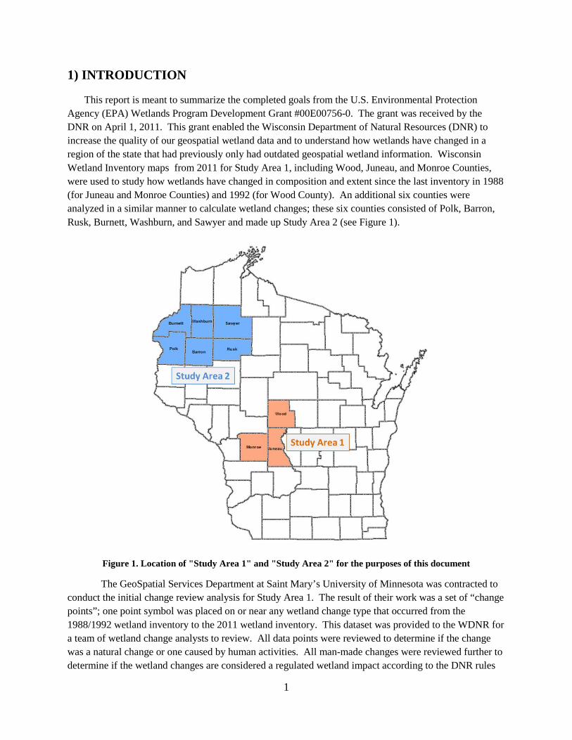
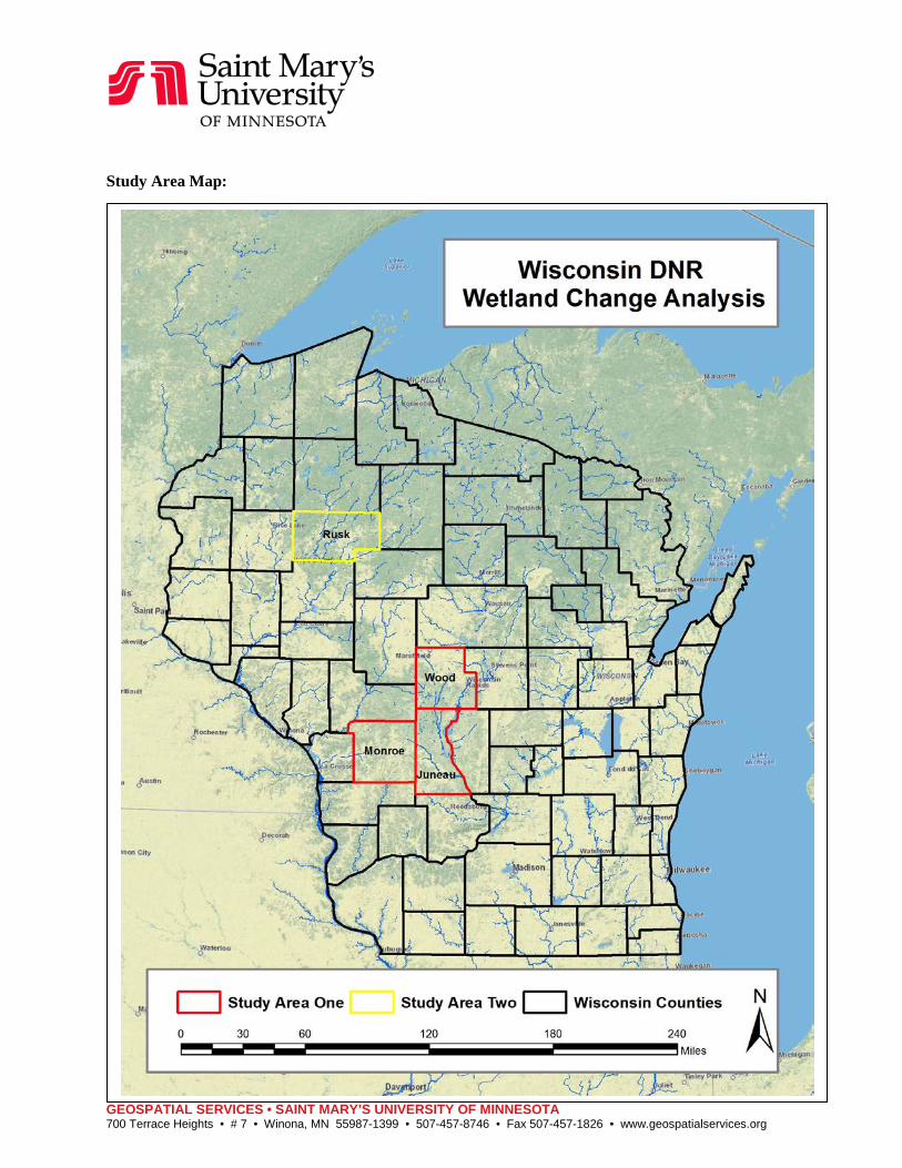
This report is meant to summarize the completed goals from the U.S. Environmental Protection Agency (EPA) Wetlands Program Development Grant #00E00756-0. The grant was received by the DNR on April 1, 2011. This grant enabled the Wisconsin Department of Natural Resources (DNR) to increase the quality of our geospatial wetland data and to understand how wetlands have changed in a region of the state that had previously only had outdated geospatial wetland information. Wisconsin Wetland Inventory maps from 2011 for Study Area 1, including Wood, Juneau, and Monroe Counties, were used to study how wetlands have changed in composition and extent since the last inventory in 1988 (for Juneau and Monroe Counties) and 1992 (for Wood County). An additional six counties were analyzed in a similar manner to calculate wetland changes; these six counties consisted of Polk, Barron, Rusk, Burnett, Washburn, and Sawyer and made up Study Area 2 (see Figure 1).
Figure 1. Location of "Study Area 1" and "Study Area 2" for the purposes of this document
The GeoSpatial Services Department at Saint Mary’s University of Minnesota was contracted to conduct the initial change review analysis for Study Area 1. The result of their work was a set of “change points”; one point symbol was placed on or near any wetland change type that occurred from the 1988/1992 wetland inventory to the 2011 wetland inventory. This dataset was provided to the WDNR for a team of wetland change analysts to review. All data points were reviewed to determine if the change was a natural change or one caused by human activities. All man-made changes were reviewed further to determine if the wetland changes are considered a regulated wetland impact according to the DNR rules
1
and regulations. For any regulated impact that we determined to be unpermitted, we created a regulatory review file (RRF) to show the timing of the impacts, landscape attributes, location of 1988/1992 and 2011 wetlands, and landowner information.
We also conducted a review of wetland changes in Study Area 2 that was similar to Saint Mary’s review of the changes in Study Area 1. In Study Area 2, our intentions were to attempt to create an automated system to identify significant wetland changes and to further identify on a large-scale which of those changes may be regulated impacts. The Saint Mary’s University review for Study Area 1 was time consuming so the intention of the DNR review for Study Area 2 was to determine if we could devise an automated method to locate significant possibly-regulated wetland losses and conversions.
2) PROJECT GOALS
The primary goal of this grant was to investigate how wetlands have changed in amount, extent, and in composition in the west-central (Study Area 1) and north-western regions (Study Area 2) of Wisconsin over the last two decades. Another goal was to use that information to help inform public policies by understanding what activities are most commonly impacting wetlands. In addition, the wetland change data was used to determine if wetland impacts were regulated activities or naturally occurring changes. Finally, this project gathered background data on activities that were found to be regulated and unpermitted by either the Department of Natural Resources (DNR) or the U.S. Army Corps of Engineers (USACE).
A secondary goal of this grant was to obtain new wetland coverage for Study Area 1, Wood, Juneau, and Monroe Counties. In addition, Marathon and Portage Counties had aerial photos taken in the spring of 2015 using this grant funding. The first phase of this grant was to collect leaf-off stereoscopic aerial photographs of these three counties which were used to delineate and then digitize current wetland data into the Wisconsin Wetland Inventory. Another goal would be to use the results of this project for educational purposes by reaching out to groups that were found to be impacting wetlands without first getting a permit from the DNR or the USACE. Finally, grant funds were used to train DNR staff in wetland field techniques; 55 staff were trained in wetland plants and soils and another 35 staff were trained in how to complete the Wisconsin Rapid Assessment Methodology wetland assessment tool.
3) ANALYSIS OF WETLAND CHANGES IN STUDY AREA 1: WOOD, JUNEAU, AND MONROE COUNTIES
A) Introduction
Study Area 1 encompasses three counties in west-central Wisconsin, including Wood, Juneau, and Monroe Counties. Prior to the 2011 Wisconsin Wetland Inventory (WWI) mapping, the most recent Wood County WWI wetland layers were from 1992 and the most recent WWWI for Juneau and Monroe Counties was completed in 1988. It was important to obtain an updated understanding of what wetland resources are present in this region and what resources have been lost or gained. Using the older WWI (from the spring of 1988 and 1992) and the newer WWI (from the spring of 2011), we were able to compare how wetland resources have changed over the 19 to 23 year timespan.
2
Saint Mary’s University of Minnesota was sub-contracted to conduct the initial analysis of wetland changes in Study Area 1. The result of their work was a basic analysis of wetland type changes from 1988/92 to 2011 and a series of point features in ArcMap that indicate the location of wetland changes from the 1988/92 WWI to the 2011 WWI.
Using the data Saint Mary’s University staff compiled on these changes, we further analyzed wetland change trends and reviewed each wetland change point to determine if the activity was regulated or not. If we identified a regulated impact, we determined if the activity was permitted by the DNR and/or the U.S. Army Corps of Engineers (USACE). All regulated, potentially unpermitted activities were further investigated to determine when the impact occurred, who currently owns the land, and if there are any additional environmental resources potentially at risk as a result of the activity.
B) Wetland Change Trends
1. St. Mary’s University Analysis
The Wisconsin Department of Natural Resources (DNR) contracted the Wisconsin Wetland Inventory (WWI) change analysis to the Geospatial Services team at Saint Mary’s University of Minnesota. Specifically, Saint Mary’s was tasked with digitally converting wetland data for four counties, Wood, Juneau, Monroe, and Rusk, for use in the WWI. Once this conversion was completed, Saint Mary’s overlaid 1988/92 WWI layers with the new 2011 WWI layers and performed a simple intersect function in ArcMAP to determine where wetland types changed from 1988/92 to 2011. The results of this analysis can be found in Appendix A.
2. DNR Analysis and Results
In order to better understand the general wetland change trends in Study Area 1, we analyzed the raw WWI polygon change data prepared by Saint Mary’s University. This data was compiled by Saint Mary’s using ArcGIS to calculate how many acres of wetlands and what type of wetlands were lost or gained from 1988/92 to 2011 and if there were wetlands in both inventory years - if the wetland type changed from 1988/92 to 2011. This overlay analysis resulted in a list of WWI wetland type changes (class, subclass, hydrologic modifiers, and special modifiers) by county.
To understand wetland changes, we categorized wetland changes by wetland class and by special modifier. Wetland classes consist of aquatic bed (“A”), moss (“M”), emergent/wet meadow (“E”), scrub/shrub (“S”), forested (“T”), flats/unvegetated wet soil (“F”), and open water (“W”). Some additional waterway features were labeled in the WWI, such as lakes or rivers, and therefore are included here but do not represent all lakes and river acreage in Study Area 1. We decide to separate cultivated cranberry beds (“S6Kc”) from other shrub/scrub wetlands and that is indicated in the following tables (“S(c)”). The remaining acreage for the county was considered upland (although this is misleading as some of that acreage is in fact rivers or ponds/lakes).
We also categorized wetland changes by some of the WWI special modifiers, but we did not include special modifiers that did not indicate specific anthropogenic impacts (e.g. central sands complex, red clay complex, ridge and swale complex, mats, exposed flats complex, or evidence of muskrat activity). Any wetland that did not have a special modifier associated with it or had one of the non-anthropoegnic special modifiers was considered an “unmodified” wetland. The special modifiers we
3
analyzed consisted of formerly cultivated land that was abandoned (“a”), cranberry bogs (“c”), farm/cropland (“f”), grazed/pastured land (“g”), wetland where vegetation was recently removed (“v”), and excavated ponds (“x”) – these classes were called “modified” wetlands in this study indicating that they were anthropogenically altered.
Study Area 1
Study Area 1, made up of three counties, has a total area of 1,619,276.6 acres; in 1988/92, 18.4% of the region was mapped as wetland (297,286.6 acres) which increased to 24.4% (395,457.3 acres) by 2011. While there appears to be a significant increase in wetlands, we expect that many of those “new” acres may have been present in 1988/92 but were not adequately mapped as wetland at the time. More wetlands may have been mapped in 2011 due to higher quality and resolution aerial images and better soils information in this region. In addition, we observed a large increase in excavated ponds which we did not consider a naturally-occurring wetland in this analysis.
We identified that 83.3% of all community class types did not change from 1988/92 to 2011 in Study Area 1. Of the wetland classes (aquatic bed, emergent/wet meadow, flats/unvegetated wet soil, moss, scrub/shrub, and forested), we saw that 0.1% of the region (1,170.6 acres) was converted to commercial cranberry beds, 2.3% of the region (37,369.9 acres) were converted to a lower vegetative structural wetland class (e.g. forested wetland converted to shrub wetland), and 2.4% of the region (38,333.6 acres) were converted to a higher vegetative structural wetland class (e.g. emergent wetland converted to forested wetland). In addition, we observed 0.2% of the region (2,448.2 acres) converted from wetlands (WWI class types A, E, F, M, S, and T) to open water communities (WWI class type W) and 0.2% (3,848.2 acres) converted from open water to wetland. Another 3.6% of the region (42,302.1 acres) was converted from wetlands to upland and 8.2% (132,639.9 acres) converted from upland to wetland. A breakdown of each of the three counties’ breakdown in wetland class and special modifier changes can be found in Appendix A.
Table 1. Study Area 1 wetland class changes from 1988/92 WWI to 2011 WWI.
2011 Wetland Class A E F M S S (c) T W Lake River U
1. St. Mary’s University Creation of Change Points
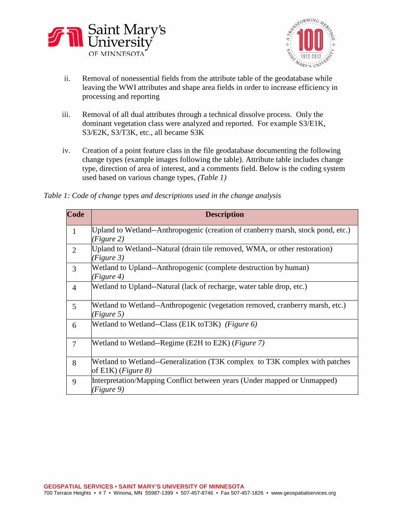
In addition to summarizing wetland change trends, Saint Mary’s University was tasked with developing a wetland change analysis process for Study Area 1. For this analysis, they identified the locations of all wetland changes in these three counties and determined what type of change took place. Saint Mary’s created a system of change categories as well as a method to mark each of the changes to describe the general change type. See Appendix B for a description of the methods Saint Mary’s University staff used to complete the wetland change analysis for the DNR.
Wetland Change Categories
The staff at Saint Mary’s University created nine wetland change categories to classify the wetland changes found in Study Area 1. Each change point created was assigned one (and occasionally more than one) wetland change category. These categories were created by determining if the change was most likely a natural occurrence or the result of anthropogenic activities. Categories were then split into how the wetland changed from the 1988/92 WWI to the 2011 WWI. The nine categories are as followed:
1) Upland Wetland, Anthropogenic – These changes were considered ones that resulted in the creation of man-made wetland or waterway feature in an area that was upland in 1988/92. Examples include the construction of cranberry beds or wildlife ponds; these features are included in the WWI even though they are not natural wetlands.
2) Upland Wetland, Natural – These changes are conversions from upland to wetland where no clear anthropogenic impacts are visible. Examples include removal or failure of drainage features, wetland restoration work, or the creation of a wildlife management area. While many of these require anthropogenic efforts, the result is a natural wetland.
3) Wetland Upland, Anthropogenic – These changes include the complete loss of wetlands that were present in 1988/92 as a direct result to anthropogenic changes to the landscape in or before 2011. Examples include draining a wetland for farming use (usually as a result of the construction of ditches or installation of drain tiles), construction of buildings, construction of roads/parking lots, or the fill of a wetland for other man-made uses.
4) Wetland Upland, Natural – These changes are ones where wetland was present in 1988/92 but not in 2011 and there are no clear indicators as to how or why the wetland was lost. Examples include a drop in the water table or the natural lack of recharge.
5
5) Wetland Wetland, Anthropogenic – These changes are observed when a more natural wetland was present in 1988/92 but was converted to an anthropogenic wetland feature by 2011. Examples include the construction of new cranberry beds, dikes, or reservoirs, the grazing of animals in wetland, or the removal of vegetative material form a wetland. The result of these activities does not drain the wetland, but converts it to an anthropogenically altered or constructed wetland.
6) Wetland Wetland, Class Change – This change type is when a wetland is converted from one WWI class category or subclass of wetland to another WWI class from 1988/92 to 2011. Classes in the WWI include aquatic beds, moss communities, emergent/wet meadows, scrub/shrub, forested, flats/unvegetated wet soil, or open water less than six feet deep. Subclasses in the WWI differ based on which class they are associated with, but generally differ based on the dominant plant species of the wetland. An example of a wetland class change type would be when an emergent/wet meadow community converts to a forested community, or vice versa.
7) Wetland Wetland, Regime Change – This change type is when a wetland of the same class and usually subclass (as defined above in #6) undergoes a conversion from one WWI wetland regime to anther WWI wetland regime from 1988/92 to 2011. Regimes in the WWI refers to the hydrologic modifiers and include: a) standing water/lake, b) flowing water/river, c) standing water, palustrine, and d) wet soil, palustrine. An example of this change type would be the conversion of an emergent wetland with standing water to an emergent wetland with wet soil.
8) Wetland Wetland, Resolution Issue – This change type was used to categorize the issue of a change in how structurally mixed wetland communities were categorized in the past and how they are currently categorized. Historically, these wetland complexes were delineated as one wetland and grouped into one larger category type showing a mixed community (e.g. T5/E1K indicating that the community was mostly forested with patches of emergent wetland). But more recently, mappers have begun to separate these two types out into separate polygons with separate community type descriptions (e.g. a larger polygon of T5K with smaller polygons labeled as E1K). In this example, the maps would show a conversion of a forested community, T5/E1K, to an emergent community, E1K, even though no landscape changes can be visible.
9) 1988/92 2011 Interpretation or Mapping Issue – This change type, similar to type #8 above, was used to describe wetland ‘changes’ that were the result of newer and better mapping technologies in 2011 than were available in 1988/92. This category was used to describe a number of examples where no real change was visible between aerial images in 1988/92 and the aerial images in 2011. An example of this would be a very small pond present in 1988/92 that was not mapped at that time that but was then identified in the 2011 WWI; this would be considered a wetland gain but in reality, no real change had occurred. There were also cases where a pond was included in the 1988/92 WIW as a point symbol but then delineated as a polygon in 2011; again this would indicate a gain in wetland acreage even though the extent of the pond borders had not changed since 1988/92.
6
Establishment of Points
The Geospatial Services staff at Saint Mary’s University overlaid the 1988/92 WWI layer with the 2011 WWI layer and using the intersect tool in ArcMAP, created a new layer of polygons that listed both the 1988/92 and 2011 wetland types. After pulling out the wetland polygons that had undergone a change from 1988/92 to 2011, they created one point at the center of each wetland change polygon. This series of points became the wetland change points that we based the majority of our analysis on. If a wetland change could likely be viewed from a nearby public road, the point was placed on the road with a directional qualifier indicating the location of the wetland change. In addition, Saint Mary’s assigned a change category (1-9, see above for details) to each change point. A total of 15,590 points were created by Saint Mary’s (see Figure 2 for their distribution across Study Area 1). A complete report on the results of the Saint Mary’s change study is attached in Appendix C. Figure 2 shows a map of Study Area 1 with wetland change points in blue.
Figure 2. Distribution of change points across Study Area 1
7
2. DNR Review of Change Points
Using the set of wetland change points created by Saint Mary’s University of Minnesota, we reviewed each point to identify if the activity is a regulated activity or not. Due to the nature of the change points in categories 8 and 9 (the categories showing resolution issues and mapping issues), we did not review these points in our detailed map review; there were 3,967 change points in categories 8 and 9. To accomplish our review of change points labeled as types 1-7, we divided up all wetland change points between the three DNR wetland change analysts.
Our first task was to identify if the change highlighted was one that is a regulated activity or not. If the activity was a regulated one, we checked to see if the activity correlated with a permit in the DNR waterway and wetland permit database (see section 3.D. below for more information on the DNR permit database review). We added additional points to the map if we discovered any significant un-marked wetland changes (41 points). We also added points if there were any new excavated ponds or dammed ponds more than 1,000 feet from a change point and more than 100 feet from a 1988/92 WWI pond symbol (1,333 points). All combined, we reviewed 16,956 wetland change points in Study Area 1.
Any change points that were determined to not represent any form of activity regulated by the DNR or the U.S. Army Corps of Engineers (USACE) were labeled as “unregulated.” Any activities that appear to have matched up well with a DNR wetland permit were labeled as “permitted.” A handful of change points we identified in the DNR permit database as already under some form of enforcement and therefore were labeled as “enforcement.” All points that appeared to have regulated changes and did not match up with a permit in the database were labeled as “unpermitted.” See Figure 3 for a breakdown in the location of these points.
Figure 3. Location of unregulated, permitted, enforcement, and unpermitted (RRF) change points.
8
The remaining points represent those that we determined were most likely a regulated activity and that we could not find any associated DNR wetland or waterway permit. With this final set of unpermitted points, we identified the amount of wetland impact and the current landowner. We combined change points that were associated with the same landowner and from physically adjacent parcels of land for later use when compiling “Regulatory Review Files” (hereafter referred to as “RRFs”). Each wetland change point that was regulated and unpermitted was labeled with the name of the RRF.
3. Results
Study Area 1
Of the 16,902 wetland change points, we determined that almost 20% of the points (18.7%, 1,465 points) fell into change category 6, wetland class changes. If we group change categories 6 and 7, we find that 26.8% of all change points were the result of some form of natural wetland conversion over time. Another 32.6% of all wetland changes (5,518 points) were resolution, interpretation or mapping issues (change categories 8 and 9) likely resulting from the change in technology and common practices from the 1988/92 WWI surveys to 2011 WWI. Taken together, the wetland changes and interpretation issues (change categories 6 through 9) accounted for almost 60% of the change points (59.3%, 9,994 points). The remainder of the points fell into categories 1 through 5 or were some combination of categories. Categories 1, 3, and 5 were determined by Saint Mary’s to be the result of anthropogenic activities; these change points accounted for 26.2% of all points (4,427 points). The naturally occurring change categories, 2 and 4, accounted for only 8.7% of all change points (1,470 change points). Finally, 6.0% of all change points (1,011 points) were described as a combination of more than one change category, mostly a combination of categories 6 and 7. See Table 9 for a breakdown of change points by county.
Table 3. Number and percent of wetland change points in each change category.
Change Category: Wood Juneau Monroe Total (Sum of three counties)
Categories 3 and 4 both represent a loss of wetland acreage or a conversion from wetland in 1988/92 to upland in 2011 (3.8% of wetland change points, 643 points). Categories 1 and 2 represent a gain in wetland acreage or a conversion from upland in 1988/92 to wetland in 2011; these changes
9
represented 22.9% of all change points (3,871 points). While this may indicate that this region experienced a large increase in the overall acreage of wetlands, we determined that that is most likely not the case. The quality of aerial images has increase quite a bit from 1988/92 to 2011 and may account for smaller or more isolated wetlands being ‘picked up’ by WWI reviews. In addition, change category 1 appears to show an increase in wetlands, but many of these points and the acreage associated with those points are the gain in artificial wetlands and dammed or excavated ponds. This large increase in open water and man-made wetlands is included in the WWI but does not represent an increase in naturally functioning wetlands.
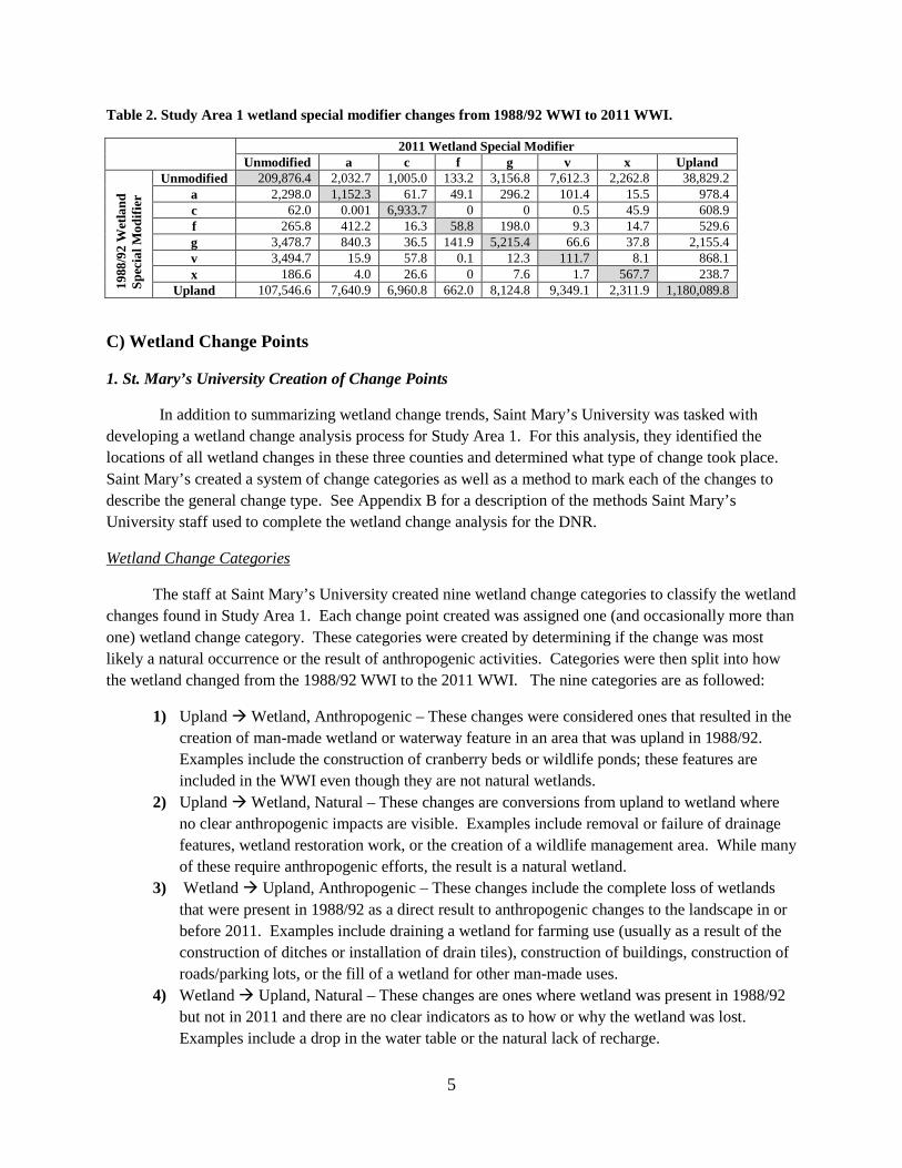
Figure 4. Number of regulated change points by county
Wood
The 6,580 Wood County wetland change points were evenly distributed among most of the change point categories except the category 4 (wetlandupland, natural) which only had five of the county’s change points. The most change points were of categories 6 and 9 (wetlandwetland class change and interpretation/mapping issues, respectively) with both of these categories representing over 1,200 change points each. There were 2,053 change points representing anthropogenically impacted wetlands (categories 1, 3, and 5).
We identified that 599 wetland change points out of 5,680 points were regulated activities. Of those, we determined that 50 points had corresponding permits in the DNR Waterway and Wetland Permit Database. Another 35 points we found corresponding activities in the same database but were listed as previously under some form of enforcement. The remaining 514 wetland change points were determined to be regulated and unpermitted by the DNR. An RRF was created for 346 points and another
0
100
200
300
400
500
600
700
Wood Juneau Monroe
Num
ber o
f Cha
nge
Poin
ts
County
Permitted
Enforcement
Unpermitted, No RRF
Unpermitted, RRF
10
168 change points were determined to be unpermitted, but we did not create an RRF for these points (mostly because they represented very small wetland impacts).
Juneau
Saint Mary’s University identified 6,502 wetland change points for Juneau County. Similarly to Wood County, almost half of those points were for category 6 and 9 (wetland class changes and interpretation/mapping issues). There were 1,184 change points for categories 1, 3, and 5, indicating an anthropogenic wetland change.
Of these wetland change points, we determined that 6,115 of those points were unregulated changes, leaving 387 regulated activities. Of the regulated changes, we determined that 69 were previously permitted by the DNR and another 5 were previously under some form of enforcement. The remaining 313 wetland change points we determined were regulated and unpermitted. The majority of these, 232 points, we determined warranted the creation of an RRF and 81 we determined were of such small impact that no RRF was needed at this point.
Monroe
A total of 3,820 wetland change points were identified by Saint Mary’s University of which most of these wetland change points were labeled as change types 1, 6, and 9 (uplandwetland – anthropogenic, wetland class change, and interpretation/mapping issues). The rest of the points were evenly divided between the different change categories except category 4 (having 0 points). Anthropogenic wetland change points (categories 1, 3, and 5) accounted for 1,190 points which is 26.2% of the change points identified.
Of the 3,820 change points, 87.3% of those changes (3,334 points) we determined were the result of unregulated activities. We identified 101 of those change points were permitted by the DNR and another 31 points were previously under some form of enforcement or another. The remaining 354 points we determined were a result of some form of regulated activity. Of those points, we determined 231 were of significant impact enough to create an RRF for these wetland impacts.
D) Compliance Monitoring Preparation
1. DNR Permit Review
Most of the projects that were identified as being permitted were reviewed in the DNR field offices located in LaCrosse, WI and Black River Falls, WI. We were able to compare the wetland impacts evident from aerial photos and the WWI with the maps and delineations submitted as part of DNR permit files. Often the acreage of impacts did not align up perfectly with what was permitted. Most often, this was because a delineation did not identify wetlands in the exact same areas as were determined on WWI aerial images. For these situations, we determined that the on-the-ground delineation would be used instead of the WWI delineated boundary. In other cases, it appeared the landowner applied for permission to do part of the work in wetlands but not the entire site that was impacted. In these cases, we created an RRF for the portion of the work that appeared to be unpermitted and referenced the permit number for the remainder of the permitted activities.
11
2. COE Permit Review
The DNR requested a list of U.S. Army Corps of Engineers (USACE) permits for Study Area 1, Wood, Monroe, and Juneau Counties, from 1988 to 2011. The Corps provided us a list of all waterway and wetland permits, informal activities, some enforcement activities, pre-application meetings, and a few applications that were determined to not be regulated by the USACE. The DNR does not track any waterway or wetland impacts associated with any Wisconsin Department of Transportation (WisDOT) projects in the DNR Waterway and Wetland Permit Database but these are tracked by the USACE as any other wetland impact; this prevents us from comparing the DNR database to the USACE database directly. These permits were checked against the Study Area 1 wetland change points and against the DNR waterway and wetland permit database. A total of 762 database entries were included in the USACE file (which included entries for pre-applications that did not result in a permit and entries for un-regulated activities) of which we found a match to DNR-database entries for 479 of those (63%). That leaves 283 entries (37%) unmatched to any file in the DNR database. We determined that many of the unmatched database entries (216 of the 283 unmatched permits, 76%)) were likely related to Wisconsin Department of Transportation (WisDOT) activities. Additional analyses of the databases can found in Appendix D.
There are limitations to this comparison, mostly in the completeness of the USACE and the DNR databases, but there are also differences in data entry (e.g. the USACE uses latitude/longitude to locate the activity location and the DNR historically used mainly the Public Land Survey System) and labeling of permit activities and permit applicants. These differences often made it difficult to match the federal and state permits with complete confidence. Both databases include the option of including the other agency’s permit number for easier cross-referencing, but this field was often left blank by the USACE and the DNR.
The list of USACE permit database entries included 762 entries of which we determined 91.5% (697 entries) were for permitted activities (this excluded entries for enforcement, exemptions, unregulated activities, and pre-application meetings). We found a matching activity in the DNR Waterway and Wetland permit Database for 479 of the USACE database entries (62.8%). This means that around 40% of the activities tracked by the USACE were not found in the DNR database. We identified 283 USACE database entries (37.1% of all entries) that were associated with road construction projects; we found a match for 67 of those entries indicating that they may have been associated with local road projects which are not regulated by WisDOT. The remaining 216 entries for road projects may be found in the WisDOT database, but we did not requisition those files for review for this grant. We identified 414 permits issued by the USACE and were able to find matching permits for 90.0% of those (371 permits); the remaining 43 USACE had no matching DNR permit (not including any possible WisDOT permits). See Appendix D for a breakdown of the types of unmatched USACE permits.
3. Regulatory Review File Creation
A detailed file was created for each site that had potential unpermitted activities that appeared to have significantly impacted wetland resources. The intent of these files was to prepare background information such as historic photos, location information, and detailed wetland information about these sites that could be used by regulators to further investigate these changes on the ground. We created a total of 494 RRFs that represent a potential of up to 2,778 impacted wetland acres. The name of each
12
Regulatory Review File, or “RRF,” was made up of the county where the impact occurred, the township, range, and section of the impact location, and the last name or business name of the current landowner (e.g. “Wood_24N03E04_Jarosz” or “Monroe_16N03W_JaroszTruckingInc”).
Each RRF file was created to include a wide range of information that is informative about the type of wetland change observed. Information contained in each RRF included the following:
1) The location of the wetland change was shown using the Public Land Survey System (PLSS) as well as the latitude and longitude of the impacts. With the PLSS, we listed the township, range, and section. If the entire impact site was contained within a single quarter or quarter-quarter, that was listed as well. Finally, the wetland change point identification number assigned by Saint Mary’s was listed so that it could easily be found if the user has access to the ArcGIS maps.
2) The type of wetland change observed was characterized using the wetland change category as defined by Saint Mary’s University of Minnesota (see section 3.b.2) as well as a list of the 1988/92 WWI community type and the 2011 WWI community type.
3) We described the type of wetland change in more detail by detailing the probable type of landscape changes and how that may have impacted, directly or secondarily, the 1988/92 wetland. We also calculated, to the best of our ability, the primary and secondary wetland impacts. Primary impacts were considered those that were found to have been lost or converted by direct anthropogenic actions and secondary impacts were losses or conversion of nearby wetlands as a likely result of primary impacts.
4) We also identified the current landowner according to the counties’ land records. In addition to the landowner name, we listed the wetland impact parcel identification number and the current landowner’s mailing address (note that this is not always the physical address of the wetland impact location). In some of the more updated RRF files, historic landownership was tracked down to the time that the impact(s) occurred.
5) Multiple aerial images from historic images from Farm Service Agency (FSA) aerials, National Agriculture Imagery Program (NAIP) aerials, and Wisconsin Regional Orthography Consortium (WROC) aerial images in addition to the WWI images from 1988/92 and 2011. The images were used to pinpoint the year in which any impacts were observed.
6) Each RRF files also contained recent aerial images showing the 1988/92 and 2011 WWI polygon and point features. These two layers are overlaid into one image with the 24K hydrologic (rivers, streams, and other water features) and the PLSS section lines.
7) In addition, each RRF also showed a recent aerial image with the wetland impacts highlighted. The highlighted section describes the type of change and the amount of wetland impacted.
8) Finally, some RRFs with more recent and larger wetland impacts were expanded to include additional information such as excerpts from the Bordner Survey and historic USGS maps. We also added recent aerial images with GIS layers laid over the aerial including: wetland indicator soils, floodplains, designated waters (Areas of Special Natural Resources Interest, Public Rights Features, and Priority Navigable Waterways), and 24K digital raster graphics (topographic maps).
13
4. Results
In order to collect information on any suspected activities that were unpermitted by the USACE or DNR, we created a Regulatory Review File (RRF), for each site. Since the initial analysis of each of these activities was done using digital, desk-top tools, each RRF was for only supposed unpermitted activities; in order to confirm that these sites were in fact unpermitted or even a regulated change at all, we conducted a review of the actual permit files (usually located in the district offices). To more thoroughly understand the real impacts, would have needed to conduct an on-site, field review of each site. Therefore, the RRF’s referred to here, list details about potential unpermitted activities that have not been ground-truthed. Each RRF contains information about the location and nature of the unpermitted activity, current landowner name and address, location of the 1988/1992 wetlands, location of the 2011 wetlands, and a series of aerial images showing the timing of any landscape changes that might have impacted existing wetlands or waterways.
A total of 494 RRFs were created for all three counties in Study Area 1: 226 for Wood County, 125 for Juneau County, and 117 for Monroe County. These RRFs represent a total of 2,778.3 acres of wetland impacts. We divided wetland and waterway impacts into one of six categories: 1) conversion of a higher wetland class to a lower wetland class, 2) activities associated with commercial cranberry operations, 3) development of a non-permeable structure (e.g. parking lot, building), 4) construction of a pond, 5) draining of a wetland that converts a wetland to a permeable upland site, and 6) a catch-all category of any activities that did not fit into one of the other five categories. The majority of RRFs (323), were for pond construction in a wetland or within 500 feet of a waterway which impacted a total of 440.6 acres of wetland. The category that represented the most acres of wetland impact was the commercial cranberry operations; while we only created 100 RRFs for this category, the cranberry category totaled 1,965.6 acres of wetland impacts (71% of all RRF wetland impacts). A detailed analysis of the RRF categories and associated wetland impacts can be found in Appendix E.
Table 4. The number of RRFs and the percentage of all RRFs by general category and county.
Conversion Cranberry Development Pond
Wetland to Upland Other Total
Wood Number 2 44 8 162 19 1 236
Acres 18.1 525.5 9.8 203.5 84.4 0 841.3
Juneau Number 4 13 4 98 10 1 130
Acres 18.7 566.3 15.87 157.5 29.59 78.9 866.9
Monroe Number 1 43 11 63 9 1 128
Acres 7.2 873.8 71.9 79.6 35.2 2.4 1,070.1
Total Number 7 100 23 323 38 3 494
Acres 44.0 1,965.6 97.6 440.6 149.2 81.3 2,778.3
After determining which points are regulated points and which were not, we determined that 8.7% (1,472 points) of all the change points (16,902 points) represented a regulated activity. Of those 1,472 regulated activity points, 19.7% of those points were either previously permitted or already under enforcement. The remaining 80.3% of change points were associated with regulated activities that we
14
could not find a corresponding DNR permit or enforcement action in the DNR Waterway and Wetland Permit Database. Of those unpermitted, regulated change points, we created a Regulatory Review File (RRF) for 809 of those points. We determined that the remaining 372 unpermitted, regulated change points were of such small or minor impacts that it did not warrant the creation of an RRF.
While the majority of the RRFs we created were for the construction of new ponds (323 RRFs for Study Area 1) in wetlands or within 500 feet of a stream, the projects did not represent much wetland impact in acreage (440.6 acres of wetlands impacted in Study Area 1). Commercial cranberry-related project sites had less than one third the number of RRFs (100 RRFs for Study Area 1) than ponds but had almost 5 times the number of wetland acres impacted (1,965.6 acres in Study Area 1).
Figure 5. Number of unpermitted wetland change points for Study Area 1 by general impact category
Figure 6. Acres of wetland impact for all unpermitted wetland change points for Study Area 1 by general impact category
0
50
100
150
200
250
300
350
400
Conversion Cranberry Development Pond WL Restoration WL to UL Enforcement Permitted Other
Num
ber o
f RRF
s
Impact Category
WoodJuneauMonroe
0
100
200
300
400
500
600
700
800
Conversion Cranberry Development Pond WL Restoration WL to UL Enforcement Permitted Other
Acre
s of W
etla
nd Im
pact
Impact Category
WoodJuneauMonroe
15
Wood
Wood County had the most RRFs of any of the three counties in Study Area 1 with 244 files which totaled 944.6 acres of wetlands lost or impacted. The majority of the RRFs were for man-made ponds in wetlands or within 500’ of a waterway; these activities counted for 229.8 acres of wetland impacts. There were 40 RRFs associated with commercial cranberry operations which totaled 513.3 acres of impacted wetlands. Cranberry impacts counted for 54.3% of all Wood County unpermitted activities. The remaining quarter of wetland acreage impacts were for conversion, development, wetland-to-upland, and other activities.
The largest impact was for a cranberry site which had five wetland change points and had wetland impacts totaling 124.2 acres of wetland impacts. Many of the RRFs for Wood County were for wetland impacts that were much smaller. Seventy-five RRF files totaled wetland impacts of less than 1 acre per site. Twenty-four RRF files had wetland acreage impacts greater than ten acres per site. Sixty RRFs were created that had no impacts and were for ponds that were constructed in upland but that were within 500 feet of a waterway.
Juneau
The 229 unpermitted change points were combined into 131 RRFs which accounted for 931.1 acres of unpermitted wetland impacts. The vast majority of RRFs (77% of all RRFs in Juneau County) were created for the construction of ponds in wetland or near waterways. These 101 pond RRFs accounted for 136.2 acres of wetland impacts which is only 14.6% of the total unpermitted wetland impacts in Juneau County. The pond-related RRFs averaged 1.3 acres of wetland impact per site. The majority of wetland impacts were associated with commercial cranberry operations, with a total of 534.3 acres of unpermitted wetland impacts at only 12 sites which is an average of 44.5 acres per cranberry site. There were also 12 RRFs totaling 114.5 acres of wetland loss associated with the drainage of wetland and 6 RRFs associated with large scale wetland conversion for 534.3 acres of wetland impacts.
The largest impact was for a cranberry operation which involved 15 wetland change points and involved wetland impacts from 1991 through 2010. Many of the RRFs we created for Juneau County had small impacts, including 60 files that involved impacts less than 1 acre in size per site. An additional 23 RRFs had zero wetland impacts; all of these RRFs were for new ponds constructed within 500 feet of a waterway.
Monroe
We created 120 RRFs for the 199 unpermitted wetland change points. These 120 files were associated with 938.9 acres of wetland impacts. Similarly to Wood and Juneau Counties, over half of the RRFs created for Monroe County were for the construction of new ponds but the average size of these impacts was 1.1 acres per site. Again, the vast majority of wetland impacts (79.6%) were associated with 35 RRFs for commercial cranberry operation sites. There were another 12 RRFs, totaling 121.7 acres of wetland impacts, for conversion, development, wetland drainage, and ‘other’ categories.
The largest impact in Monroe County was for a cranberry operation site and contained 9 wetland change points totaling 89.09 acres of wetland impacts. Of the 120 RRFs, 18 of those had wetland impacts
16
less than 1 acre and another 35 RRFs had no wetland impacts, all of which were ponds constructed within 500 feet of a waterway.
4) ANALYSIS OF WETLAND CHANGES IN STUDY AREA 2: BURNETT, WASHBURN, SAWYER, POLK, BARRON, AND RUSK COUNTIES
A. Introduction
For this analysis, we focused on six counties in northwestern Wisconsin: Burnett, Washburn, Sawyer, Polk, Barron, and Rusk Counties. The WWI was updated for these counties in 2002 or in 2004. Because of the older timespan and larger area, this analysis is more limited in scope than the analysis conducted in Chapter 1 for Study Area 1. The cause of wetland impacts was determined, but not the timing of the impacts. We did not attempt to determine whether wetland impacts were regulated or whether permits were obtained.
One goal of the analysis was to create a model in ArcGIS to evaluate wetland changes in lieu of reviewing each wetland change point-by-point as was done in Chapter 1 for Study Area 1. GIS was used to summarize the acreage of wetland changes based on the class and special modifier codes used in the wetland inventory, as well as to filter out some sources of error. However, the GIS model was not effective in distinguishing between natural and anthropogenic causes of wetland losses, so comprehensive review of aerial photos and other GIS layers by an analyst was necessary to identify and measure likely wetland drainage or fill. Because 1978/79 point features were not digitized for the counties Study Area 2, it was not possible to use GIS to compensate for differences in minimum mapping unit between years. A subset of aerial photos for each county was reviewed to determine what proportion of the gain in wetland area was due to wetlands previously mapped as point features.
B. Methods
1. Data sources and limitations
As shown in Table 1, successive updates to the WWI have differed in the type of imagery available and in some of the mapping procedures used. When comparing wetland acreage between years, these procedural differences must be taken into account. WWI air photo interpreters use 9x9 inch, 1:20,000 scale black and white infrared aerial photos, viewed in stereo, to identify and map wetlands. Recent updates to the inventory (2002 and 2004) used photographs taken in spring before vegetation had leafed out. This type of photography is preferred for identifying forested wetlands that would otherwise be hidden by the leaf canopy. The original inventory had access only to leaf-on images taken during the summer, so forested wetlands were likely underreported. Aquatic beds and non-persistent emergent vegetation are generally mapped as open water in leaf-off photos, as these plants do not emerge above the water until later in the growing season. The time of year that photographs were taken may also account for changes in hydrologic modifier and areal extent of some wetlands. For example, a wetland that is flooded by spring rains and snowmelt and that dries up during the summer would be given a “wet soil” hydrologic modifier in the leaf-on inventory and a “standing water” hydrologic modifier in the leaf-off inventory.
17
Map unit size also differed between inventories. Wetlands, excavated ponds, and dammed ponds that are too small to be delineated on 1:20,000 scale photographs are indicated with symbols. While these features may be digitized as point data in GIS, they do not contribute to estimates of wetland area. The original inventory employed a minimum mapping unit (MMU) of 2 or 5 acres, depending on the county (see Table 1). The use of an explicit minimum mapping unit was dropped in recent updates. Air photo interpreters were consistently able to delineate wetlands larger than 1 acre, and sometimes as small as tenths of an acre, depending on the shape and context. Because of the change in map unit size, many wetlands and ponds mapped as point features in 1978/79 were mapped as polygons in 2002 or 2004, contributing to an apparent increase in wetland acreage.
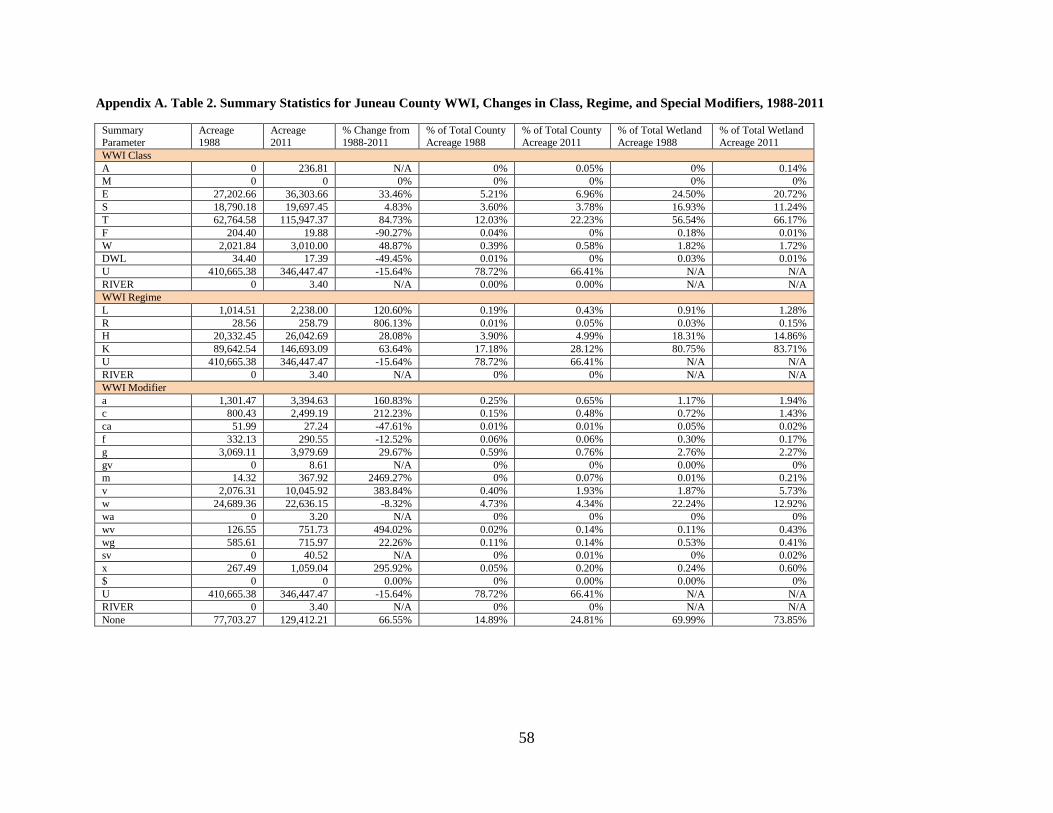
Table 5: Wisconsin Wetland Inventory metadata, Study Area 2
1978/1979 WWI 2002/2004 WWI County Date of
inventory Type of imagery used
Ortho-rectified?
Minimum mapping unit
Date of inventory
Type of imagery used
Ortho-rectified?
Minimum mapping unit
Barron 1978-1979 B&W infrared, leaf-on
Partially 2 acres 2004 B&W infrared, leaf-off
Yes Not defined*
Polk 1978-1979 B&W infrared, leaf-on
Partially 5 acres 2004 B&W infrared, leaf-off
Yes Not defined*
Rusk 1978-1979 B&W infrared, leaf-on
No 5 acres 2004 B&W infrared, leaf-off
Yes Not defined*
Burnett 1978-1979 B&W infrared, leaf-on
Yes 5 acres 2002 B&W infrared, leaf-off
Yes Not defined*
Sawyer 1978-1979 B&W infrared, leaf-on
No 5 acres 2002 B&W infrared, leaf-off
Yes Not defined*
Washburn 1978-1979 B&W infrared, leaf-on
No 5 acres 2002 B&W infrared, leaf-off
Yes Not defined*
*No minimum mapping unit is explicitly set. Air photo interpreters were asked to delineate the smallest wetlands possible, which, depending on the shape of the wetland, was frequently tenths of an acre.
2. Correction of alignment
In some areas, 1978/79 wetland maps fail to align with current GIS data because of differences in the coordinate system used, digitization errors, and distortions present in base maps that were not ortho-rectified. These issues were corrected to the extent practicable to allow for comparisons between years.
The Wisconsin DNR now uses the Wisconsin Transverse Mercator (WTM) projection referenced to the NAD83 HARN geodetic control as the common coordinate system for all its GIS data. However, 1978/79wetland data from Washburn and Burnett counties appear to have been stored in WTM referenced to an older geodetic control, NAD27. This projected coordinate system is displaced by 200 meters
18
relative to NAD83, and legacy file formats are missing the information necessary for GIS software to correct the discrepancy. Wetland data for these counties were re-projected into WTM NAD83 HARN.
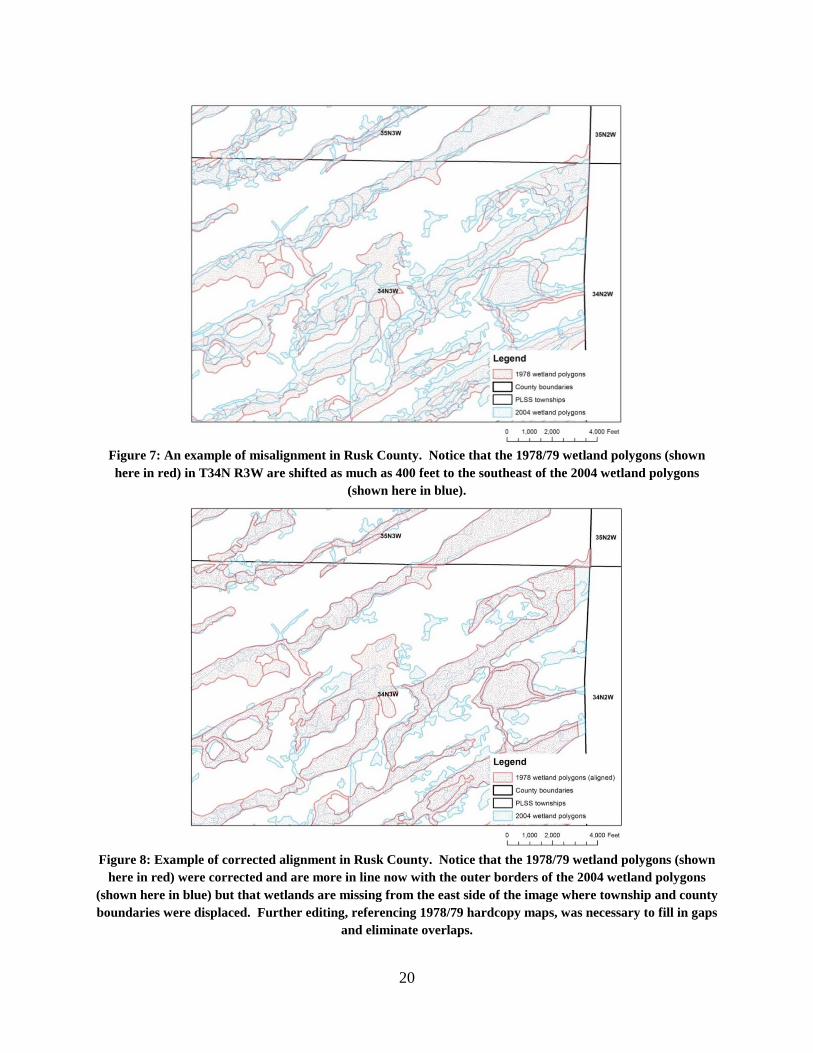
In certain townships, the 1978/79 wetland polygons were displaced by as much as 400 feet relative to current wetland polygons (see Figure 1), most likely due to the use of basemaps that were not orthorectified. Current wetland inventory maps are digitized directly from the interpreted 1:20,000 scale aerial photos and orthorectified using OrthoMapper software. Prior to the migration of the inventory to a digital format, wetland maps were drafted on 1:24,000 scale photographic mylar basemaps, usually centered on and covering a public land survey system (PLSS) township. USGS orthophotoquads were used as basemaps for the portions of the state where they were available—including Burnett County and portions of Polk and Barron counties. However, the photographs used as basemaps for the rest of the state were not orthorectified and can include large positional errors due to camera tilt and relief displacement. Additional positional error appears to have been introduced during digitization; if a map included few road intersections for ground control, georeferencing was inaccurate. When older wetland inventory maps were digitized, the goal was wetland acreage rather than spatial accuracy; orthorectification and edge-matching were not attempted, so discontinuities are evident along the boundaries between townships.
A projective transformation was used to correct alignment in each township showing severe displacement (see Figure 2). Due to the lack of “well-defined” points such as road intersections in the affected areas, control points also included the center points of distinctive features such as small wetlands, peninsulas, and lake inlets that could be matched between years. This procedure significantly improved alignment, but some errors as large as 80 feet remain. By comparison, National Map Accuracy Standards (USGS, 1947) require that 90% of control points on a 1:24,000 topographic map or orthophotoquad be within 40 feet, so wetland acreage and changes will be more accurate in counties where orthophotography was available. In some townships, tens of acres of wetlands mapped on hardcopy aerial photos were revealed to have been cropped out of the digital inventory or duplicated during digitization as a result of misalignment; editing was performed along township and county boundaries to merge overlapping polygons and to fill in gaps greater than 40 feet.
19
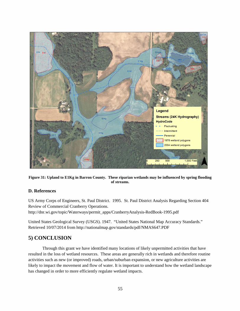
Figure 7: An example of misalignment in Rusk County. Notice that the 1978/79 wetland polygons (shown here in red) in T34N R3W are shifted as much as 400 feet to the southeast of the 2004 wetland polygons
(shown here in blue).
Figure 8: Example of corrected alignment in Rusk County. Notice that the 1978/79 wetland polygons (shown
here in red) were corrected and are more in line now with the outer borders of the 2004 wetland polygons (shown here in blue) but that wetlands are missing from the east side of the image where township and county boundaries were displaced. Further editing, referencing 1978/79 hardcopy maps, was necessary to fill in gaps
and eliminate overlaps.
20
Due to budget limitations, some parts of the 1978/79 wetland inventory for Burnett County had been digitized as generalized wetland complexes, with wetland-upland boundaries shown, but without labels or boundaries between different wetland types. Using hardcopy wetland inventory maps as reference, we used editing tools to separate and label wetlands with a special modifier indicating human influence or indicating upland inclusions. This allowed total wetland losses and anthropogenic disturbances to be characterized for the county.
3. GIS overlay analysis
A GIS model was constructed using the Model Builder package in ESRI ArcMap to automate some of the analysis of wetland changes. Wetland polygons from current and older inventories were overlaid for each county using a union operation, allowing the acreage of each change to be measured and aggregated. Only polygons could be compared using GIS, as 1978/79 wetlands represented as point features were never digitized for these counties. A sample of aerial photos was reviewed to identify 2002/2004 polygons that were previously mapped as point features; this is described in part D.
The wetland inventory specifically excludes large areas of open water or submerged aquatic vegetation in the primary channels of rivers or in lakes greater than six feet deep. As with uplands, these features are only indicated on the digital inventory if they are completely surrounded by wetland; blank areas on the digital inventory could be either upland or open water. To eliminate this confusion, unmapped deepwater features were distinguished from upland by selecting perennial lakes and rivers from the 24K hydrography database (waterbodies mapped on 1:24,000 scale topographic maps) and merging them with both wetland layers through another union operation (see Figure 3).
Figure 9: Example of deepwaterwetland change. Open water features from 24K USGS maps (dark blue)
were used to distinguish deepwaterwetland changes (hatched lines) from uplandwetland changes. Rooted, floating aquatic beds on the north and west sides of the lake have increased in area from 1978/79 to
2002. Because the lake is deeper than 6 feet, open water areas are not mapped as wetland.
21
Wetland changes were aggregated by cover type (wetland class) and by anthropogenic disturbance (wetland special modifier). Special modifier codes indicating a human influence were extracted from the wetland classification: these include abandoned cropland (labeled with an “a” modifier), cranberry bogs (“c” modifier), farmed (“f” modifier), grazed (“g” modifier), vegetation recently removed (“v” modifier), or excavated (“x” modifier). Abandoned cranberry beds (“c” and “a” modifier) were grouped with abandoned cropland; there were no other wetlands in these counties with two human influence special modifiers.
The class code indicates the uppermost layer of vegetation (or unvegetated wet soil or open water) which covers 30% or more of the map unit. Wetlands with a dual class (e.g. T3/S3K) were reported based on the taller vegetation type (e.g. T3/S3K would be reported as T). We observed that changes in wetland class were frequently due to more detailed mapping in the current inventory rather than changes in vegetation or hydrology. For example, an area mapped in 1978/79 as a mixed class, S3/E2K, might be mapped as separate stands of S3H and E2H in 2004 (see Figure 4). In this analysis, the change from a mixed class to its secondary component was treated as a resolution issue if the current polygon was smaller than the former polygon, and if there was no change in special modifier to indicate an anthropogenic disturbance (e.g. a change from T2/S6K to S6Kc would be considered an anthropogenic disturbance and not a resolution issue).
Figure 10: Example of resolution issues in Rusk County. An area mapped as mixed covertypes (S3/E2K) in 1978/79 has been mapped as separate shrub (S3Kw) and emergent (E2Hw) wetlands in 2004. The change
from wet soil (K) to standing water (H) may be a seasonal change in hydrology; the absence of the floodplain modifier (w) in 1978/79 is likely an oversight.
While the classification system used in the WWI contains four components (class, subclass, hydrologic modifier, and special modifier), changes to the subclass and hydrologic modifier were not
22
analyzed in this investigation. Since the photos used for interpretation were taken during different seasons (summer of 1978/79, spring of 2002 and 2004), changes in the hydrologic modifier may reflect normal seasonal variation in water levels rather than indicating a change between years so this modifier was not included in this analysis. Changes in subclass will often reflect the difference between leaf-on and leaf-off imagery so this modifier was also not included in this analysis.
Change polygons smaller than 0.05 acres were treated as slivers and excluded from analysis for this investigation. Even where no change has occurred on the landscape, small differences between inventories in the shape and size of wetland polygons are to be expected, given the precision of the source imagery. Seasonal variations in hydrology, gradual wetland-upland transitions, uncorrected displacement in images that were not orthorectified, and improvements in digitization methods also contribute to differences in the boundaries of unchanged wetlands.
Figure 11: Example of sliver polygons smaller (shown in pink). Changes smaller than 0.05 acres cannot be
distinguished from spurious differences in linework, given the scale of the source imagery and the precision of the digitization process.
4. Aerial photo review to identify wetland losses caused by anthropogenic activity
It was not possible to reliably distinguish between naturally occurring wetland losses and anthropogenic causes of wetland loss using the available GIS data. Preliminary GIS models incorporated landcover data from the National Landcover Database (NLCD) to identify former wetlands that had been converted to development or cropland. In order to test the effectiveness of this modeling, we compared the results of the model to the results of our in-depth analysis of wetland impacts in Study Area 1 (Wood, Juneau, and Monroe Counties). Of the 11 wetland sites in Juneau County filled for development prior to
23
2006, only five were correctly shown as developed landcover in the 2006 NLCD. The 30 meter resolution of NLCD data was too coarse, and classification insufficiently accurate to be used at the small scale of analysis required for this study. Therefore, we identified possible anthropogenic causes of wetland loss through visual review of aerial photos, wetland inventory polygons, and other GIS data, as was done in Study Area 1.
Wetland losses caused by human activity were identified through systematic screening of aerial photography in ArcGIS (See Figure 6), a process taking less than an hour per township. Wetland upland changes were displayed over 2005 NAIP orthophotos (2002 and 2004 orthophotos were not available). At a scale of 1:10,000, man-made features were visible and an entire PLSS section could be viewed at one time. If a wetland loss coincided with buildings, roads, ditches, artificial ponds, farm fields, or other manmade features, hardcopy wetland inventory photos were reviewed to confirm that the feature was present in 2002/2004 and not present in 1978. The hydric soils layer from the NRCS soil survey was also reviewed; in some cases, the pattern of wetlandupland changes was more consistent with revisions to the wetland inventory based on improved soil maps than with wetland fill (see Figure 7). One of several data sources used during the wetland mapping process to ensure accuracy, detailed NRCS soil surveys were not available in 1978/79 for Burnett, Washburn, Sawyer, and Rusk counties.
24
Figure 12: Example of screening for anthropogenic causes of wetland loss. Roads and buildings in areas of wetland loss (red) were identified in GIS using 2005 NAIP image. A hardcopy 1978/79 photo (inset) was
reviewed to confirm that a change had occurred.
Figure 13: Example of wetland “losses” related to improvements in soil mapping. Although wetlandupland changes (shown in orange) coincide with a new road, the losses do not occur where the road crosses a hydric soil unit (shown in pink). Black arrows indicate areas where the shape of wetland losses closely matches the
boundaries of upland soils, suggesting that these changes represent a revision from wetland to upland rather than wetland fill.
25
If the wetland loss appeared to be the result of human activity, primary impacts were measured to nearest 0.1 acre in GIS. These include any excavation or discharge of fill into former wetlands, such as new structures, roads, ditches, artificial ponds, piles of sand or gravel, and dredge spoils. Open areas that were likely graded during construction, such as lawns and disturbed ground near new roads or structures, were also treated as primary impacts. Clearing of vegetation was not considered a primary impact unless there were signs of grading, grubbing of stumps, or other large-scale soil disturbance. Certain wetlandwetland changes involve potential discharge of fill into wetlands; these were identified in GIS using special modifiers and treated as a primary impact if review of aerial photographs confirmed that the farm field, cranberry bog, or excavated pond was not present in 1978/79. While secondary impacts due to drainage ditches and other hydrologic alterations are likely, they could not be easily distinguished from natural wetland losses and mapping issues. In most cases, the wetlandupland polygon was irregular in shape and included areas of undisturbed vegetation too far from new structures or ditches to be attributed only to drainage.
Wetland losses were grouped into the following categories:
• Rural development • Incorporated development • Highways • Forestry (logging roads and trails) • Mining • Excavated ponds • Cranberry production • Agriculture (row crops)
Development includes buildings of all types, parking lots, golf courses, local roads, and driveways. 2004 minor civil divisions were used to separate development occurring within an incorporated village or city from development occurring in rural areas (unincorporated towns). County, state, and federal highways were distinguished from local roads using GIS road layers from the Wisconsin Department of Transportation. Unpaved roads not mapped by the DOT and associated with undeveloped forest areas were assumed to be logging roads, although some could be ATV or snowmobile trails. These were placed in a separate category, as they are generally exempt from wetland regulations. Excavated areas associated with piles of sand or gravel were classified as “mining” unless they occurred within cranberry operations. With the exception of the Flambeau copper mine in Rusk County, only non-metallic mining operations were present in the study area. Ponds actively used for mining of gravel and other mineral resources are specifically excluded from the WWI unless they support vegetation, so should appear in this category as wetlandupland changes rather than as wetlandwetland changes grouped with excavated ponds.
Excavated ponds were identified in GIS by selecting 2002/2004 polygons labeled with the special modifier “x- excavated” in GIS. It was not feasible to review ponds mapped as point features or dammed ponds and flowages. Wetlandupland changes adjacent to ponds were also included in this category, if changes to landform and vegetation suggested grading or placement of spoil material in wetland. Primary impacts associated with cranberry production include the beds (mapped as S6Kc), reservoirs (mapped as W0Hx), and associated dikes, pumphouses, and sand piles (mapped as uplands). Primary impacts due to
26
agriculture include farmed wetlands (special modifier “f”) and farmed uplands where the 1978/79 wetland class was forested or scrub/shrub, under the assumption that grubbing of stumps must have occurred to permit farming. Conversion of emergent/wet meadow to farmland was only treated as primary impact only if new drainage ditches or drainage tiles could be observed and measured in NAIP images, or if wetlands were marked as “$- drained/filled” in the either the 1978/79 or 2002/2004 wetland inventory (these were field-checked).
5. Aerial photo review to account for changes in the minimum mapping unit
Because of the change in map unit size, wetlands and artificial ponds that are smaller than 5 acres (or 2 acres, in Barron County) may have been mapped as point features in 1978/79 and mapped as polygons in 2002 or 2004. Since 1978/79 point features were never digitized for the counties in Study Area 2, a review of hardcopy wetland inventory materials was necessary to distinguish this kind of mapping difference from uplandwetland changes.
The 1978/79 wetland inventory was initially mapped on 9x9 inch black and white infrared photos. Since each 9x9 inch aerial photo contains four PLSS sections, the sections provided a convenient grid for sampling. PLSS sections were clipped to the county of interest using ArcGIS, setting XY tolerance to 1 meter to avoid creation of sliver polygons where county and section layers do not perfectly align. While most PLSS sections are approximately 1 square mile in area, some sections used for the sampling grid are smaller due to cropping at the state border or due to survey adjustments at the north edge of some townships. Since the objective was to determine the proportion of wetland gains previously mapped as point features rather than total acreage, variation in plot size was not a concern. The sample frame was PLSS sections containing uplandwetland changes. 5% of sections meeting this criterion were selected for each county. A union operation between PLSS sections and the output from the model described in Part C allowed the acreage of wetlandupland changes in each section to be determined.
As part of the GIS model described in Part C of this chapter, 2002/2004 wetland polygons smaller than 5 acres that did not intersect a 1978/79 wetland polygon were flagged as potential mapping issues. An analyst compared each of these polygons to hardcopy aerial photos (See figure 8). If a wetland symbol was marked on 1978/79 aerial photos at approximately the same location (as determined from physical features visible at both dates and on position relative to 1978/79 wetland polygons), an uplandwetland change could be ruled out. The mean acreage of mapping issues per section and the standard error were then normalized by the mean area of uplandwetland changes per section, to determine the proportion of the increase in wetland area that could be attributed to changes in the minimum mapping unit.
27
Figure 14: Comparison of potential mapping issues (crosshatched polygons at left) with 1978/79 hardcopy (right). Most of the 2002 wetland polygons smaller than 5 acres were present in 1978/79 but mapped as point features. 76% of the increase in wetland area for this section is due to the change in the minimum mapping unit.
C. Results
1. Study Area 2 Summary
Between 1978/79 and 2002/2004, the acreage mapped as wetland increased in each of the six counties in Study Area 2 (See Table 2). For the six-county region as a whole, the acreage mapped as wetland increased by 19% (110,337 acres). However, some of the increase can be attributed to differences in mapping between the two inventories (see Table 3). Based on review of WWI photographs from a sample of public land survey system (PLSS) sections in each county, approximately 18% of apparent gains were due to changes in the minimum mapping unit. Wetland smaller than 5 acres (or 2 acres, in Barron County) were often mapped as polygons in 2002/2004 and point features in 1978/79. When this and other mapping issues in Table 3 are excluded, the net gain is 77,399 acres (a 13% gain).
The differences between leaf-on images in 1978/79 and leaf-off images in 2002/2004 create uncertainty as to the real extent of wetland gains. Some forested and shrub wetland mapped in 2002/2004 may have been present in 1978/79 but hidden by the canopy in leaf-on images. Seasonal variations in hydrology may affect the extent of wetlands mapped in the summer of 1978/79 versus the spring of 2002 or 2004. However, our findings of a net gain in wetland acreage are also supported by an analysis of wetland gains and losses due only to anthropogenic factors. Wetland losses due to human impacts were identified from aerial photographs and totaled 1112.8 acres for the region. Changes from upland to wetlands with the special modifier “a- abandoned”—an unambiguous measure of wetland gains due to restoration or other changes in management—totaled 2,793.1 acres. Since these areas were formerly cultivated land, they should have been visible as wetland in leaf-on images if present in 1978. By these measures, the six-county region showed a net gain of 1680.3 acres of wetland due to human activity, but Washburn and Sawyer counties had net losses. Anthropogenic causes of wetland gain and wetland loss are discussed in greater detail below.
Based on special modifiers, 3561.4 acres of wetland gains (1.8%) can be attributed to human activity (see Table 4). Cranberry beds are considered wetlands, although they lack the diverse plant community and most of the functions and values associated with natural wetlands (US Army Corps of Engineers, 1995). 233.2 acres of artificial cranberry bogs were constructed in uplands. 535.1 acres of excavated ponds appear to have been constructed in uplands, although this number includes ponds that were present in 1978/79 and mapped as point features. “Excavated ponds” may or may not have the functional values associated with natural wetlands, as this category includes ponds and “scrapes” constructed specifically for wildlife habitat, as well as relatively barren stock ponds, landscape ponds, and deep cranberry ditches. The special modifier “a- abandoned” is used for wetlands where old plow lines and fence lines are still visible, but that show no evidence of recent cultivation. Based on this modifier, 2,793.1 acres of farmed upland were restored to wetland or were abandoned and reverted to wetland between 1978/79 and 2004. Grazed, logged, and farmed wetlands were not included in Table 4, as these
Wetland Gain/LossAcres gain/loss
Percent of total gain/loss
*UplandWetland (actual) 157,889 77.9%*UplandWetland (smaller than minimum mapping unit, mapped as point feature in 1978) 36,362 17.9%DeepwaterWetland 7,320 3.6%Slivers (changes less than 0.05 acres) 1,215 0.6%Total wetland gains 202,787 100.0%WetlandUpland 80,490 87.1%WetlandDeepwater 8,636 9.3%Upland inclusions in Central Sands complex (j) 2,291 2.5%Slivers (changes less than 0.05 acres) 1,032 1.1%Total wetland losses 92,449 100.0%Net gain 110,337 *Estimate, based on random sample of PLSS Sections
Gain
sLo
sses
29
activities are not likely to introduce wetland hydrology. Not all artificial or restored wetlands will be mapped with a special modifier. If no fence lines or signs of excavation are visible, wetland restoration projects, dammed ponds, and flowages could be mapped as E2H, W0H, or W0L; this was sometimes observed in Study Area 1. Dead trees (“T7”) in wetland are frequently associated with dammed reservoirs and flowages, although they can also be the result of natural flooding along streams, beaver ponds, high winds, and other factors; there were 2,672 acres of uplandT7 changes in the region. However, human activities are still likely to be a small component of wetland gains. As seen in Figure 9, the majority of uplandwetland changes (120,253 acres) were mapped as forested wetland in 2002/2004.
Table 8: Acres of uplandwetland change attributed to human activity, based on 2002/2004 special modifier
2002/2004 special modifier County a –Abandoned (acres) c- Cranberry bog (acres) x- Excavated (acres) Barron 760.2 66.1 Polk 503.5 105.3 Rusk 880.6 8.6 58.4 Burnett 520.2 17.0 88.6 Sawyer 75.6 108.8 102.5 Washburn 53.0 98.8 114.2 TOTAL 2,793.1 233.2 535.1
Figure 15: Uplandwetland changes by 2002/2004 covertype class, 6-county region
Based on review of aerial photos, there were 1112.8 acres of primary impacts to wetlands in the 6-county region. This includes wetlandupland changes where new structures, new drainage features, or grading could be observed, as well as wetlandwetland changes involving potential discharge of fill material and loss of functional values. Additional wetland losses may be due to secondary impacts from drainage ditches or other alterations to hydrology, but these could not easily be distinguished from natural
A- Aquatic Bed 0%
E- Emergent / Wet meadow
16% F- Flats/ Unvegetated
Wet Soil 0%
S- Scrub/ shrub 20%
T- Forested 62%
W- Open Water 2%
30
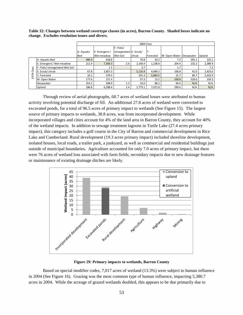
changes and mapping errors. While human impacts account for only 1.2% of gross wetland losses, they are of special concern from a regulatory standpoint. The largest anthropogenic cause of wetland losses in the region was cranberry production, affecting 541.8 acres (See Figure 10). This figure excludes dammed cranberry reservoirs unless they were mapped with the special modifier “x-excavated.” 90% of the impacts were associated with a few large operations in Sawyer and Washburn counties; there were no active cranberry bogs in Barron or Polk counties. Development accounted for 17% of primary impacts, with 78.4 acres occurring inside of municipal boundaries (as of 2004) and 114.0 acres occurring outside. In these largely rural counties, much of the development pressure affecting wetlands has been from cabins, houses, and campgrounds along lakeshores. Agriculture caused 159.7 acres of primary impact through clearing and leveling of forested and shrub wetland and through new drainage structures in farmed wetlands or emergent/wet meadows. Highways, forest roads, and non-metallic mining were minor sources of primary wetland impacts, affecting 31.5 acres, 17.5 acres, and 9.0 acres, respectively.
Figure 16: Causes of primary impacts to wetland, Study Area 2
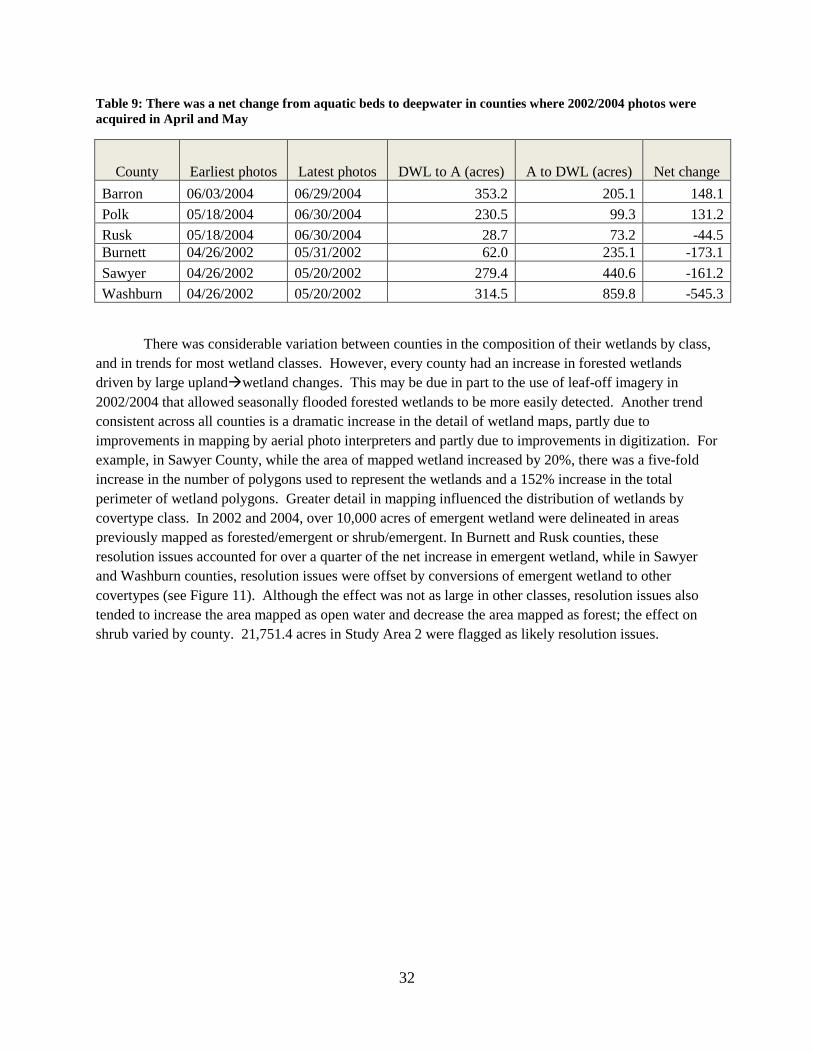
Wetlanddeepwater changes accounted for 9.3% of gross wetland losses in the six-county area (See Table 3). While wetlanddeepwater changes were generally offset by deepwaterupland changes and had little effect on total wetland acreage, they were sometimes the largest factor influencing the acreage of aquatic beds, open water wetlands, or emergent/wet meadows. Note that a change between wetland and deepwater features does not necessarily indicate a gain or loss in littoral habitat (e.g. through dredging, sedimentation, or permanent change in water level). In a lake with maximum depth greater than six feet, large areas of open water or submerged vegetation are not mapped as wetland, so any change in the extent of emergent vegetation or floating aquatic vegetation will appear as a change in wetland area; this could be due to browsing or pest pressure, management of aquatic plants in lakes, changes in water quality, or year-to-variations in hydrology. Seasonal factors are also involved, as areas mapped as aquatic beds or non-persistent emergent vegetation in the summer are generally mapped as open water when viewed in the spring, before leaves of aquatic plants reach the surface of the water. In counties where aerial photos were acquired in April and May of 2002, there was a net shift from aquatic beds to open water in deepwater lakes (See Table 5).
Table 9: There was a net change from aquatic beds to deepwater in counties where 2002/2004 photos were acquired in April and May
County Earliest photos Latest photos DWL to A (acres) A to DWL (acres) Net change Barron 06/03/2004 06/29/2004 353.2 205.1 148.1 Polk 05/18/2004 06/30/2004 230.5 99.3 131.2 Rusk 05/18/2004 06/30/2004 28.7 73.2 -44.5 Burnett 04/26/2002 05/31/2002 62.0 235.1 -173.1 Sawyer 04/26/2002 05/20/2002 279.4 440.6 -161.2 Washburn 04/26/2002 05/20/2002 314.5 859.8 -545.3
There was considerable variation between counties in the composition of their wetlands by class, and in trends for most wetland classes. However, every county had an increase in forested wetlands driven by large uplandwetland changes. This may be due in part to the use of leaf-off imagery in 2002/2004 that allowed seasonally flooded forested wetlands to be more easily detected. Another trend consistent across all counties is a dramatic increase in the detail of wetland maps, partly due to improvements in mapping by aerial photo interpreters and partly due to improvements in digitization. For example, in Sawyer County, while the area of mapped wetland increased by 20%, there was a five-fold increase in the number of polygons used to represent the wetlands and a 152% increase in the total perimeter of wetland polygons. Greater detail in mapping influenced the distribution of wetlands by covertype class. In 2002 and 2004, over 10,000 acres of emergent wetland were delineated in areas previously mapped as forested/emergent or shrub/emergent. In Burnett and Rusk counties, these resolution issues accounted for over a quarter of the net increase in emergent wetland, while in Sawyer and Washburn counties, resolution issues were offset by conversions of emergent wetland to other covertypes (see Figure 11). Although the effect was not as large in other classes, resolution issues also tended to increase the area mapped as open water and decrease the area mapped as forest; the effect on shrub varied by county. 21,751.4 acres in Study Area 2 were flagged as likely resolution issues.
32
Figure 17: Effect of resolution issues (S/EE and T/EE) on acreage of emergent/wet meadow.
i. Polk
In 1978/79, wetlands made up 12.9% of Polk County’s 597,088 acres. Between 1978/79 and 2004, our GIS analysis shows a loss of 10,248 acres and a gain of 26,584 acres, for a net gain of 16,335 acres (see Table 6 and Table 7). However, the net gain shrinks from a 26.8% increase to a 13.4% increase when changes to the minimum mapping unit, vegetation changes in deepwater lakes, and sliver polygons are excluded. Based on review of 46 PLSS sections randomly sampled from Polk County, 28% (±5%) of apparent uplandwetland changes (by area) were actually wetlands smaller than 5 acres that were mapped as point features in 1978/79 and polygons in 2004. In addition, some of the gain may be due to wetlands that were present in 1978/79 but not visible in leaf-on imagery, however, this is difficult to quantify.
Table 10: Wetland acreage by cover type class, Polk County
Resolution issue (separated from mixed class) Other factors
33
Table 11: Wetland gains and losses, Polk County
Forested wetlands were the most common wetland class in both years (See Table 6). Forested wetland increased by 47.8%, due largely to change from uplands (11,607 acres, see Table 8). However, “uplandwetland” changes include wetlands that were present in 1978/79 but that were not visible through the tree canopy in leaf-on imagery, as well as wetlands smaller than 5 acres that were present but mapped as point features in 1978. Shrub wetlands declined by 31.9%, due to succession to forest (4,964.6 acres), changes to emergent vegetation (3,264.4 acres) and changes to upland (2,196.0 acres). Emergent/wet meadow increased by 77.1%, largely due to change from upland (8,556.0 acres). Open water increased by 43.6%, but changes from upland (976.1 acres) may be ponds smaller than 5 acres that were mapped as point features in 1978, while changes from deepwater (547.6 acres) appear to be shallow ponds that were mistakenly omitted in 1978. Aquatic beds declined by 18.9%, largely due to changes to emergent marsh (789.3 acres).
Table 12: Changes between wetland covertype classes (in acres), Polk County. Shaded boxes indicate no change. Excludes resolution issues and slivers.
A review of aerial photos identified 39.1 acres of wetland loss that could be attributed to human activities. Another 24 acres of wetland were converted to excavated ponds for a total 58.6 acres of primary impacts to wetlands (see Figure 12). Excavated ponds, such as stock ponds, landscape ponds, and wildlife scrapes, caused 63.1 acres of primary impact, although this does not include small ponds mapped as point features. Rural development accounted for 21.1 acres of primary impact. In addition to houses and cabins, this category includes 3.9 acres of fill for a golf course, 1.0 acre for an RV/trailer park,
Wetland Gain/Loss Acres Percent of gain/loss*UplandWetland (actual) 17,663 66.4%*UplandWetland (smaller than minimum mapping unit, mapped as point feature in 1978) 6,869 25.8%DeepwaterWetland 1,912 7.2%Slivers (changes less than 0.05 acres) 139 0.5%Total wetland gains 26,584 100.0%WetlandUpland 9,530 93.0%WetlandDeepwater 609 5.9%Slivers (changes less than 0.05 acres) 110 1.1%Total wetland losses 10,248 100.0%Net gain 16,335 *Estimate, based on random sample of PLSS Sections
2.0 acres of commercial development, and 1.0 acre fill for a shooting range. Another 7.6 acres of fill for development occurred within the City of Amery and within the villages of Luck and Clayton. 17 acres of wetland were cleared for agriculture, including 7 acres of primary impact from grubbing and clearing of forested and shrub weltands and from excavation of drainage features. Other categories accounted for less than 5 acres of primary impact.
Figure 18: Primary wetland impacts, Polk County
Based on special modifier codes, 5,512 acres of wetland (7.1%) were subject to human influence in 2004. Grazing was the most common form of human influence, affecting 3,057 acres (see Figure 13). While the acreage of grazed wetlands almost tripled, this appears to be due primarily due to changes from upland (net 2,279.4 acre, see Figure s), rather than grazing of previously undisturbed wetland (net 703.7 acres). Since grazing is common in floodplains, the change from upland to grazed wetland might be partially explained by seasonal differences in hydrology between the spring of 2004 and summer of 1978. 503.5 acres of farmed upland were abandoned and reverted to wetland (Upland”a”); this could include wetlands restored through conservation programs. Other forms of human influence were uncommon.
0.0
5.0
10.0
15.0
20.0
25.0
30.0
Wet
land
impa
ct (a
cres
)
Conversion toupland
Conversion toartificialwetland
35
Figure 19: Acreage of wetland with a special modifier indicating human influence, Polk County
Table 13: Changes between special modifiers indicating human influence (in acres), Polk County. Shaded boxes indicate no change. Excludes resolution issues and slivers.
ii. Burnett
Table 14: Wetland acreage by covertype class, Burnett County
In 1978/79, wetlands made up 24.3% of Burnett County’s 525,248 acres. Between 1978/79 and 2002, our GIS analysis shows a loss of 20,479 acres and a gain of 26,055 acres, for a net gain of 5,781 acres (see Table 26 and Table 27). Net gains are revised only slightly to a 4.1% increase when mapping differences are excluded, as this county has some major issues associated with wetland losses, as well as wetland gains. 2,382 acres of wetland were reclassified as deepwater features, partly because of changes in vegetation on deepwater lakes, and partly depth information was unavailable for many lakes in 1978. 2,291 acres of apparent wetland losses were due to better delineation of uplands within areas previously mapped as wetland/upland complexes (see Figure 24). The glacial outwash plain found in Burnett County contains areas of wet sand and peat intermingled with dry sand ridges that are difficult to interpret using leaf-on photography, so were mapped with the special modifier code “j—Central Sands complex” in 1978. During the 2002 update to the inventory, the “j” modifier was not used, as leaf-off imagery made it easier to distinguish wetland from upland in these areas. Based on review of 44 PLSS sections randomly sampled from Burnett County, 18% (±2%) of apparent uplandwetland changes (by area) were actually wetlands smaller than 5 acres that were mapped as point features in 1978/79 and polygons in 2002. In addition, some of the gain may be due to wetlands that were present in 1978/79 but not visible in leaf-on imagery, however, this is difficult to quantify.
Table 15: Wetland gains and losses, Burnett County.
Wetland Gain/Loss Acres Percent of gain/loss*UplandWetland (actual) 20,479 78.6%*UplandWetland (smaller than minimum mapping unit, mapped as point feature in 1978) 4,495 17.3%DeepwaterWetland 898 3.4%Slivers (changes less than 0.05 acres) 183 0.7%Total wetland gains 26,055 100.0%WetlandUpland 15,436 76.1%WetlandDeepwater 2,382 11.7%Upland inclusions in Central Sands complex (j) 2,291 11.3%Slivers (changes less than 0.05 acres) 164 0.8%Total wetland losses 20,274 100.0%Net gain 5,781 *Estimate, based on random sample of PLSS Sections
Gain
sLo
sses
37
Figure 20: Mapping issues specific to Burnett County. Central sand complexes ("j' special modifier) include
forested uplands that were difficult to delineate with 1978/79 leaf-on images. In some areas, only wetland-upland boundaries were digitized; wetlands are represented as generalized complexes (“WET”).
Due to budget limitations, some parts of the 1978/79 wetland inventory for Burnett County had been digitized as generalized wetland complexes, with wetland-upland boundaries shown but without labels or boundaries between different wetland types. While this complicates our efforts to characterize changes in wetland vegetation, conclusions can still be drawn from Table 28, supplemented by general observations from review of hardcopy materials.
Based on review of hardcopy maps, the areas digitized as generalized wetland changed little from 1978/79 to 2002 except for a few small successional changes and some changes from vegetation to open water due to water level management in wildlife areas. Much of the 3,215.2 acres of generalized wetland converted to upland appear to be forested areas that were revised based on improved soil information. The remaining generalized wetland areas were mapped as 40% scrub, 30% emergent, 25% forested, 3% open water and 2% aquatic bed in 2002. Forested wetland was underrepresented compared to the county in 2002 (38% of wetlands were forested) or compared to labeled wetlands in 1978/79 (39% were forested). This is probably due to the inclusion of most of the 30,000 acre Crex Meadows Wildlife Area, dominated by sedge meadow (E) and shrub carr (S).
If generalized wetland areas are excluded, the largest WetlandWetland changes were successional changes from scrub to forest (5978.1 acres) and from emergent to scrub (4241.1 acres, see Table 28). Natural succession, combined with large UplandWetland changes (12,641.0 acre), contributed to the increase in forested wetland. While WetlandWetland changes decreased the acreage of emergent wetland by 1,957.9 acres and shrub wetland by 849.4 acres, large UplandWetland changes
38
(6870.8 acres for scrub, 4,931.4 acres for emergent) contributed to an overall increase in these categories. However, the large increase in emergent wetland seen in Table 26 can be partially attributed to resolution issues, which caused net increase of 4,349.1 acres at the expense of shrub and forested wetland. Open water wetlands increased due to changes from upland (480.4 acres) and from other wetland types (net 517.6 acres) but some of these were present in 1978/79 and mapped as point features. Aquatic beds declined, due largely to changes to open water in deepwater lakes (235.1 acres) and changes to emergent wetland (160.6). The use of leaf-off photography in 2002 may explain part of the decline, as aquatic beds are generally mapped as open water in early spring.
Table 16: Changes between wetland covertype classes (in acres), Burnett County. Shaded boxes indicate no change. Excludes resolution issues and slivers.
Through review of aerial photographs, 104.9 acres of wetlandupland changes could be attributed to human activity. Another 48.3 acres were converted to artificial wetland types, for a total of 153.2 acres of primary impacts (see Figure 24). Excavated ponds were the largest source of primary impacts (48.3 acres). WetlandUpland changes associated with ponds include spoil material from landscape and stock ponds, a 5.2 acre dam built in wetland as part of a DNR wildlife management project, and 5.5 acres of ditches and dikes where a tamarack bog (T2/S6K) was converted to some sort of wildlife pond on private land. Agriculture caused 33.2 acres of primary impact, with most of that in a single field (27.9 acres E1Kf field checked in 2002 and labeled as filled/drained). Rural development caused 31.2 acres primary impact, mostly through development of cabins, houses, and campgrounds along lakeshores. Development in the villages of Webster and Siren accounted for 22.9 acres of primary impact, a disproportionate share considering that incorporated areas make up only 0.6% of the county. Wetland impacts in these villages included commercial buildings, athletic facilities, houses, sewage disposal ponds, and a power substation. 10 acres of wetland were filled for new cranberry beds.
Figure 21: Primary impacts to wetlands, Burnett County
Based on special modifier codes, 127,808 acres of wetland (4.9% of total wetland acreage) were subject to human influence in 2002. Grazing was the most common form of human influence, affecting 3,406 acres, a four-fold increase from 1978 (see Figure 25). 1,383.1 acres of previously undisturbed wetlands were grazed in 2002 (see Table 29). Since grazing often occurs in floodplains of streams, some of the 1,675.5 acres converted from upland may be due to seasonal differences in hydrology between summer of 1978/79 and spring of 2002. 520.2 acres of farmed uplands were abandoned and reverted to wetland; this could include restoration projects. Large changes from abandoned to undisturbed wetland (328.8 acres) and from undisturbed to abandoned (509.8 acres) may be due to differences in interpretation where plow lines and fence lines were ambiguous. 856 acres of wetland were labeled as “vegetation recently removed” in 2002; it is not clear why the modifier was not used in 1978. Excavated ponds increased from 20 to 231 acres, but much of this increase is due to ponds that were present in 1978/79 but mapped as point features. Only one quarter of wetlandW0Hx changes could be confirmed as new ponds by review of aerial photos. Farmed wetlands increased more than four-fold due primarily to changes from upland (214.7 acres); however, some of this could be due to seasonal differences in hydrology. New cranberry beds were built in upland and in wetland, but no increase is shown in Figure X because of offsetting mapping issues.
0
10
20
30
40
50
60
Wet
land
impa
ct (a
cres
)
Conversionto upland
Conversionto artificialwetland
40
Figure 22: Acreage of wetland with a special modifier indicating human influence, Burnett County
Table 17: Changes between special modifiers indicating human influence (in acres), Burnett County. Shaded boxes indicate no change. Excludes resolution issues and slivers.
iii. Rusk
In 1978, wetlands made up 19.3% of Rusk County’s 584,439 acres. GIS analysis showed a wetland gain of 49,917 acres and wetland losses of 18,009 acres for a net gain of 31,908 acres (a 28.2 percent increase; see Table 14 and 15). However, the net gain shrinks from a 28.2% increase to a 22.9% increase when changes to the minimum mapping unit, vegetation changes in deepwater lakes, and sliver polygons are excluded. Based on review of 67 PLSS sections randomly sampled from Rusk County, 12% (±2%) of apparent uplandwetland changes (by area) were actually wetlands smaller than 5 acres that were mapped as point features in 1978/79 and polygons in 2004. In addition, some of the gain may be due to wetlands that were present in 1978/79 but not visible in leaf-on imagery, however, this is difficult to quantify.
Shrub wetlands were the most common wetland class in 1978/79 but declined by 14,750 acres (29 percent), due largely to succession to forest (15,379.9 acres, see Table 16). Forested wetlands increased by 34,719 acres (69.8%), becoming the most common wetland class in 2004. The large shifts from upland to forested wetland (33,744.1 acres) and from forested wetland to upland (10,146.9 acres) can be partially attributed to the difficulty in mapping forested wetlands using leaf-on imagery. Emergent wetlands increased by 11,404 acres (102 percent). Changes from upland (7,197.1 acres) and from shrub wetland (4,229.0 acres) were the largest factors, although resolution issues (3138.5 acres previously mapped as T/E or S/E) also contributed to the increase. Open water wetlands increased, largely due to changes from upland (457.3 acres). Only 58.4 acres of new upland ponds were labeled as excavated (see Table 17), so much of the increase may be due to natural changes or ponds mapped as point features in 1978. Aquatic beds declined by 243 acres (44.3%). Conversion to emergent vegetation (192.1 acres) was the largest factor, perhaps due to changes in water levels. Several types of changes involve a loss of vegetation layers. Based on a cursory look at aerial photos, TS changes are often associated with logging while SE changes are more likely to be natural changes or differences in mapping. Water level changes along rivers, such as the damming of Hemlock Creek, caused many of the SW and Sdeepwater changes.
Wetland Gain/Loss Acres Percent of gain/loss*UplandWetland (actual) 43,177 86.5%*UplandWetland (smaller than minimum mapping unit, mapped as point feature in 1978) 5,888 11.8%DeepwaterWetland 654 1.3%Slivers (changes less than 0.05 acres) 199 0.4%Total wetland gains 49,917 100.0%WetlandUpland 17,318 96.2%WetlandDeepwater 537 3.0%Slivers (changes less than 0.05 acres) 154 0.9%Total wetland losses 18,009 100.0%Net gain 31,908 *Estimate, based on random sample of PLSS Sections
Gain
sLo
sses
42
Table 20: Changes between wetland covertype classes (in acres), Rusk County. Shaded boxes indicate no change. Excludes resolution issues and slivers.
Through review of aerial photographs, 108.6 acres of wetland losses were attributed to human activities. An additional 66.6 acres of wetland were converted to artificial wetland types, for a total of 235.4 acres of primary impacts (See Figure 18). Conversion of shrub or forested wetland to either farmed upland or to farmed wetland (e.g. E1Kf) was treated as a primary impact because it likely involves grubbing of stumps of leveling of soil in wetlands. Agriculture was the largest source of primary impacts, affecting 69.7 acres. New drainage ditches were present at several locations so secondary impacts are likely. Cranberry cultivation was the next largest category, impacting 44.2 acres of wetland. Rural development resulted in 20.8 acres of fill, mostly houses, but also driveways, trailers, farm buildings and access roads, and commercial buildings. Excavated ponds impacted 18.3 acres of wetland. Sand and gravel mining resulted in 5.5 acres of primary impact. While 8 acres of wetland were filled in 1991 as part of the Flambeau near Ladysmith, this actually appeared as a wetland gain, as the wetlands in question were mapped as point features in 1978/79 and had been restored by 1998.
Figure 23: Primary impacts to wetlands, Rusk County
Based on special modifier codes, 10,898 acres of wetland (7.5%) were subject to human influence in 2004. Grazing was the most common form of human influence on wetlands, impacting 5,600 acres in 2004 (See Figure 19). Lightly grazed areas can be difficult to detect; this probably explains the large shifts from grazed to undisturbed wetland (2,429.8 acres) and from undisturbed to grazed wetland
(1,354.6 acres, see Table 17). 3,002 acres had been recently logged in 2004, a seven-fold increase from 1978. Part of the increase may be due to the use of leaf-on imagery in 1978/79 that caused forested and logged wetlands to be undermapped. 880.6 acres of upland (presumably farmland) was abandoned and reverted to wetland (uplanda); this number may include wetland restoration projects.
Figure 24: Acreage of wetland with a special modifier indicating human influence, Rusk County
Table 21: Changes between special modifiers indicating human influence (in acres), Rusk County. Shaded boxes indicate no change. Excludes resolution issues and slivers.
iv. Washburn
In 1978/79, wetlands made up 15.3% of Washburn County’s 518,236 acres. Between 1978/79 and 2002, our GIS analysis shows a loss of 12,789 acres and a gain of 25,255 acres, for a net gain of 12,466 acres (see Table 22 and Table 23). However, the net gain shrinks from a 15.7% increase to a 7.9% increase when changes to the minimum mapping unit, vegetation changes in deepwater lakes, and sliver polygons are excluded. Based on review of 42 PLSS sections randomly sampled from Washburn County, 31% (±4%) of apparent uplandwetland changes (by area) were actually wetlands smaller than 5 acres that were mapped as point features in 1978/79 and polygons in 2002. In addition, some of the gain may
Table 23: Wetland gains and losses, Washburn County
Forested wetlands were the most common covertype class in both years (see Table 22). Forested wetland acreage increased by 25.9%, largely due changes from upland (4,914.6 acres, see Table 24). WetlandUpland changes may include wetlands that were present in 1978/79 but were not visible in leaf-on images or that were less than 5 acres and mapped as point features. Shrub wetlands were also common and increased by 9.5%, with succession to forest (6,629 acres) outweighed by changes from upland (7,639.7 acres). Emergent wetlands declined by 12.3%, largely due to succession to shrub wetland (3,123.8 acres). Aquatic beds declined by 32.3% due largely to changes to open water in deepwater lakes (859.8 acres). This may be because of the use of leaf-off imagery from spring of 2002; aquatic beds are less visible in the spring and are generally mapped as open water. Acreage of open water wetlands more than tripled, largely due to changes from upland (1,253.7 acres). Since there were only 160 acres of excavated ponds in 2002 (see Figure 23), much of the increase is likely due to ponds smaller than 5 acres that were treated as point features in 1978.
Wetland Gain/Loss Acres Percent of gain/loss*UplandWetland (actual) 16,434 65.1%*UplandWetland (smaller than minimum mapping unit, mapped as point feature in 1978) 7,383 29.2%DeepwaterWetland 1,243 4.9%Slivers (changes less than 0.05 acres) 194 0.8%Total wetland gains 25,255 100.0%WetlandUpland 10,173 79.5%WetlandDeepwater 2,452 19.2%Slivers (changes less than 0.05 acres) 165 1.3%Total wetland losses 12,789 100.0%Net gain 12,466 *Estimate, based on random sample of PLSS Sections
Gain
sLo
sses
45
Table 24: Changes between wetland covertype classes (in acres), Washburn County. Shaded boxes indicate no change. Excludes resolution issues and slivers.
Through review of aerial photographs, 43.8 acres of wetland losses were attributed to human activity. Another 215.8 acres of wetland were converted to artificial wetland types, for a total of 259.6 acres of primary impacts (see Figure 22). Cranberry operations accounted for the overwhelming majority (80.4%) of impacts, including 182.2 acres mapped as S6Kc, 9.3 acres of reservoirs mapped as “W0Hx,” and 8.9 acres of dikes, sand piles, and other fill mapped as uplands. 21.0 acres of forested and shrub wetland were cleared and leveled for crop fields, with 10.2 acres mapped as farmed wetland and 10.8 acres mapped as upland in 2002. Excavated ponds not associated with cranberry production accounted for 15.1 acres of primary impact. 12.1 acres of fill were associated with construction of Highway 53. Rural development, including commercial buildings outside of Spooner, shoreline development, driveways, and isolated houses, accounted for 8.8 acres of primary impact. Other categories account for less than five acres of impact.
Figure 25: Primary impacts to wetlands, Washburn County
Based on special modifier codes, 91,771 acres of wetland (1.3% of total wetland acreage) were subject to human influence in 2002. Grazing was the most common form of human influence, more than tripling to affect 1,401 acres (see Figure 23). Part of this seems to be due to an increase in grazing pressure on previously undisturbed wetland (431.5 acres, see Table 25), but change from upland (707.9
acres) may reflect seasonal differences in hydrology in grazed floodplains. Logging was also common, with 467 acres showing signs of recent vegetation removal. Cranberry bogs increased by 81.2% due to conversion of undisturbed wetlands (154.7 acres), conversion of farmed or formerly farmed wetlands (27.5 acres), and construction in uplands (98.8 acres). Excavated ponds increased from 0 to 160 acres, although some of this may be ponds smaller than 5 acres that were treated as point features in 1978. Based on a cursory review of aerial photos, the increase in farmed wetlands and decrease in abandoned farmed wetlands appear to be due primarily to differences between years in hydrology and interpretation rather than changes in land use.
Figure 26: Acreage of wetland with a special modifier indicating human influence, Washburn County
Table 25: Changes between special modifiers indicating human influence (in acres), Washburn County. Shaded boxes indicate no change. Excludes resolution issues and slivers.
v. Sawyer
In 1978/79, wetlands made up 24.4% of Sawyer County’s 804,180 acres. Between 1978/79 and 2002, our GIS analysis shows a loss of 22,380 acres and a gain of 56,229 acres, for a net gain of 33,849 acres (see Table 18 and Table 19). However, the net gain shrinks from a 20.8% increase to a 14% increase when changes to the minimum mapping unit, vegetation changes in deepwater lakes, and sliver polygons
are excluded. Based on review of 67 PLSS sections randomly sampled from Sawyer County, 19% (±2%) of apparent uplandwetland changes (by area) were actually wetlands smaller than 5 acres that were mapped as point features in 1978/79 and polygons in 2002. In addition, some of the gain may be due to wetlands that were present in 1978/79 but not visible on the leaf-on imagery, however, this is difficult to quantify.
Table 26: Wetland acreage by covertype class, Sawyer County
Forested wetlands were the most common wetland class in both years and increased by 48.1%, in large part because of the 42,121.6 acres of upland that converted to forested wetland (see Table 20). However, “uplandwetland” changes include wetlands that were present in 1978/79 but that were not visible through the tree canopy in leaf-on imagery, as well as wetlands smaller than 5 acres that were present but mapped as point features in 1978. Natural succession from shrub wetland to forested wetland (20,666.3 acres) contributed to the increase in forested wetland and the decrease in shrub wetland. Other cover classes were relatively uncommon, making up less than 10% of wetland area in both years. Emergent wetland declined by 1685 acres (19.2%), largely due to succession to shrub wetland (3,791 acres). Aquatic beds also declined by 19.9%, in large part due to conversion to open water in deepwater lakes (440.6 acres). This may be due to the use of leaf-off imagery from spring of 2002; aquatic beds are
Wetland Gain/Loss Acres Percent of gain/loss*UplandWetland (actual) 44,015 78.3%*UplandWetland (smaller than minimum mapping unit, mapped as point feature in 1978) 10,324 18.4%DeepwaterWetland 1,488 2.6%Slivers (changes less than 0.05 acres) 402 0.7%Total wetland gains 56,229 100.0%WetlandUpland 20,495 91.6%WetlandDeepwater 1,564 7.0%Slivers (changes less than 0.05 acres) 321 1.4%Total wetland losses 22,380 100.0%Net gain 33,849 *Estimate, based on random sample of PLSS Sections
Gain
sLo
sses
48
less visible in the spring. Open water wetlands more than doubled due largely to conversion from upland (780.3 acres), scrub/shrub (668.6 acres), and deepwater (327.8 acres), but review of aerial photos suggest that many of the ponds were present in 1978/79 and mapped as point features. Excavation of artificial ponds accounts for less than 214 acres of the increase (see Table 20).
Table 28: Changes between wetland covertype classes (in acres), Sawyer County. Shaded boxes indicate no change. Excludes resolution issues and slivers.
Through review of aerial photographs, 89.3 acres of wetland losses were attributed to human activity. Another 275.9 acres of wetland were converted to artificial wetland types, for a total of 365.2 acres of primary impact (see Figure 20). Cranberry production accounted for the overwhelming majority (78.1%) of impacts to wetlands, including 223.6 acres of beds mapped as “S6Kc,” 34.5 acres of reservoirs mapped as “W0Hx” and 27.1 acres of dikes and other fill mapped as upland. Excavated ponds and adjacent dredge spoils that were not associated with cranberry operations accounted for 24.5 acres (6.7%) of impacts. Agriculture accounted for 18 acres of impact (4.9%), with several sites mapped as “drained/filled” on the wetland inventory. Construction on State Highways 48 and 70 resulted in the loss of 13.0 acres (3.6%). 11.7 acres of wetland (3.6%) were lost for rural development, including at least 2 acres of local roads and driveways, as well as houses, parking areas, and cabins along lakeshores and rivers. Commercial and residential development within the municipal boundaries Hayward and Radisson resulted in the loss of another 6.8 acres of wetland (1.9%). Logging roads accounted for 6 acres (1.7%) of primary impacts.
Based on special modifier codes, 2,696 acres of wetland (1.4% of total wetland acreage) were subject to human influence in 2002 (See Figure 21). As described above, 223.6 acres of wetland were converted to cranberry beds, and an additional 108.8 acres of cranberry beds were constructed on uplands (see Table 21). However, while cranberry production accounted for the majority of primary impacts in Sawyer County, logging was the most common form of human influence. 1,812 acres of wetland were labeled with the special modifier “vegetation recently removed” in 2004, an eightfold increase from 1978. While improvements in mapping due to the use of leaf-off imagery may account for some of the increase (acres mapped as forested wetland increased by 48.1% during the same period), logging pressure on wetlands does appear to have increased. Grazing affected 628 acres in 2002, more than doubling, with more than half the increase (313.2 acres) occurring in areas previously mapped as upland. Seasonal differences in hydrology from summer to spring may account for some of the increase, as grazing is common along the floodplains of streams. The 214 acre increase in excavated ponds is likely overstated, as ponds less than 5 acres may have previously have been mapped as point features. Review of wetlandW0Hx changes to determine primary impacts found that almost half were present in 1978.
0
50
100
150
200
250
300
Wet
lnad
loss
es (a
cres
)
Conversion toupland
Conversion toartificialwetland
50
Figure 28: Acreage of wetland with a special modifier indicating human influence, Sawyer County
Table 29: Changes between special modifiers indicating human influence (in acres), Sawyer County. Shaded boxes indicate no change. Excludes resolution issues and slivers.
vi. Barron
In 1978/79, wetlands made up 9.5% of Barron County’s 552,248 acres. Between 1978/79 and 2004, our GIS analysis shows a loss of 8,750 acres and a gain of 18,749 acres, for a net gain of 9,999 acres (see Table 10 and Table 11). Because of the 2-acre minimum mapping unit, wetland gains due to mapping differences are not as large as in other counties. Based on review of 40 PLSS sections randomly sampled from Barron County, 8% (±2%) of apparent uplandwetland changes (by area) were mapped as point features in 1978/79 and polygons in 2002. The net gain shrinks from 23.4% to 20.1% when changes to the minimum mapping unit, vegetation changes in deepwater lakes, and sliver polygons are excluded. Some of the gain may be due to wetlands that were present in 1978/79 but not visible in leaf-on imagery, however, this is difficult to quantify.
Shrub wetlands were the most common wetland class in 1978/79 but declined by 30.2%, in large part due to succession to forested wetland (4,694.2 acres, see Table 12). Emergent wetland increased by 39.6% to become the most common wetland type in 2004, largely due to change from upland (6,598.4 acres). Forested wetland acreage doubled, mostly due to change from upland (7,672.8 acres). However, some forested wetlands may have been present in 1978/79 but not visible through the tree canopy in leaf-on imagery. Acreage of aquatic beds remained relatively stable, with change to emergent vegetation (618.8 acres) offset by change from deepwater (353.2 acres) and emergent vegetation (211.9 acres) at other locations. Open water wetlands declined by 28.7% due largely to reclassification as deepwater (529.6 acres); these appear to be ponds and lakes deeper than 6 feet that were treated as wetlands in 1978/79 because depth information was unavailable.
Wetland Gain/Loss Acres Percent of gain/loss*UplandWetland (actual) 16,122 86.0%*UplandWetland (smaller than minimum mapping unit, mapped as point feature in 1978) 1,402 7.5%DeepwaterWetland 1,124 6.0%Slivers (changes less than 0.05 acres) 99 0.5%Total wetland gains 18,747 100.0%WetlandUpland 7,537 86.2%WetlandDeepwater 1,093 12.5%Slivers (changes less than 0.05 acres) 118 1.3%Total wetland losses 8,748 100.0%Net gain 9,999 *Estimate, based on random sample of PLSS Sections
Gain
sLo
sses
52
Table 32: Changes between wetland covertype classes (in acres), Barron County. Shaded boxes indicate no change. Excludes resolution issues and slivers.
Through review of aerial photographs, 68.7 acres of wetland losses were attributed to human activity involving potential discharge of fill. An additional 27.8 acres of wetland were converted to excavated ponds, for a total of 96.5 acres of primary impact to wetlands (See Figure 15). The largest source of primary impacts to wetlands, 38.8 acres, was from incorporated development. While incorporated villages and cities account for 4% of the land area in Barron County, they account for 40% of the wetland impacts. In addition to sewage treatment lagoons in Turtle Lake (27.4 acres primary impact), this category includes a golf course in the City of Barron and commercial development in Rice Lake and Cumberland. Rural development (19.3 acres primary impact) included shoreline development, isolated houses, local roads, a trailer park, a junkyard, as well as commercial and residential buildings just outside of municipal boundaries. Agriculture accounted for only 7.0 acres of primary impact, but there were 76 acres of wetland loss associated with farm fields; secondary impacts due to new drainage features or maintenance of existing drainage ditches are likely.
Figure 29: Primary impacts to wetlands, Barron County
Based on special modifier codes, 7,017 acres of wetland (13.3%) were subject to human influence in 2004 (See Figure 16). Grazing was the most common type of human influence, impacting 5,380.7 acres in 2004. While the acreage of grazed wetlands doubled, this appears to be due primarily due to
change from upland (net 2174.8 acres), rather than grazing of previously undisturbed wetland (net 541.3 acres, see Table 13). Since grazing is common in floodplains, the change from upland to grazed wetland might be partially explained by seasonal differences in hydrology between the spring of 2004 and summer of 1978/79 (See Figure 17). 760.2 acres of farmed upland were abandoned and reverted to wetland (Upland”a”); this could include wetland restoration projects. Other forms of human influence were uncommon.
Figure 30: Acreage of wetland with a special modifier indicating human influence, Barron County
Table 33: Changes between special modifiers indicating human influence (in acres), Barron County. Shaded boxes indicate no change. Excludes resolution issues and slivers.
Figure 31: Upland to E1Kg in Barron County. These riparian wetlands may be influenced by spring flooding of streams.
D. References
US Army Corps of Engineers, St. Paul District. 1995. St. Paul District Analysis Regarding Section 404 Review of Commercial Cranberry Operations. http://dnr.wi.gov/topic/Waterways/permit_apps/CranberryAnalysis-RedBook-1995.pdf
United States Geological Survey (USGS). 1947. “United States National Map Accuracy Standards.” Retrieved 10/07/2014 from http://nationalmap.gov/standards/pdf/NMAS647.PDF
5) CONCLUSION
Through this grant we have identified many locations of likely unpermitted activities that have resulted in the loss of wetland resources. These areas are generally rich in wetlands and therefore routine activities such as new (or improved) roads, urban/suburban expansion, or new agriculture activities are likely to impact the movement and flow of water. It is important to understand how the wetland landscape has changed in order to more efficiently regulate wetland impacts.
55
In general, we calculated an increase in wetland acreage in all 9 counties that we studied within this report. While a small increase in wetland acreage may be likely due to annual precipitation differences and any long-term drought trends, we believe that it is highly unlikely that each of these counties experienced a drastic increase in wetland acreage. For Study Area 2, the large increases in wetland acreage is likely due to an under-mapped amount of forested wetlands (the older WWI imagery was taken during the summer when leaves obscured any wetlands below the forest canopy) and large minimum mapping units (from 2 to 5 acres in size) in the 1978/79 WWI. The 2002/04 WWI images were taken during the spring and before “leaf-out” in forests and shrub wetlands, allowing the inventory mappers to catch additional wetlands previously unseen. We also observed an increase in artificial wetlands such as commercial cranberry operations and small open water ponds, both of which are calculated as an increase in wetland acreage since they are mapped in the WWI, but neither of which should be included in an increase in functional wetland acreage.
The tools used to identify wetland changes in this grant ranged from an incredibly in-depth analysis of every wetland polygon, as done by Saint Mary’s University of Minnesota and the DNR in Study Area 1, to a more automated analysis, as done by the DNR for Study Area 2. We found that both tools had advantages and weaknesses. The in-depth analysis done for Study Area 1 was able to identify almost all wetland changes, anthropogenic impacts on wetlands, and locations of significant wetland gains and losses, but this strategy also took multiple people over a year to complete and even longer to follow-up on unpermitted activities. The automated analysis of Study Area 2 could be used on a larger scale in a much quicker manner as long as the user had access to ArcMap tools. The drawback to this method is a much higher level of uncertainty. A well-trained human eye will be able to catch and analyze wetland changes much better than the computer.
We recommend the use of the automated and quicker analysis method if the user has two sets of wetland data that are both of comparable quality (e.g. both sets of data are leaf-off, orthorectified, and were generated using similar approaches to minimum mapping units) and have access to ArcGIS soils and hydrology layers. Without these conditions and additional tools, we found that comparison of wetland layers from two different years was more labor intensive. This approach does not catch all possible regulated anthropogenic activity but does highlight many areas that are likely to have experienced regulated wetland impacts. But if money and time are ample, the in-depth approach is preferable as it will identify many more impacts and generally provide a better understanding of landscape changes than the automated method.
56
Appendix A. Saint Mary’s University Data Analysis of Wetland Acreage Change Appendix A. Table 1. Summary Statistics for Wood County WWI, Changes in Class, Regime, and Special Modifiers, 1992-2011
Appendix B. Saint Mary’s University of Minnesota Wetland Change Study Methods
(see attached)
63
Digital Conversion of Wisconsin Wetland Inventory and Developing a Wisconsin Wetland Change Analysis
Project Description: The Wisconsin Department of Natural Resources (WI DNR) has received funding support from the U.S. Environmental Protection Agency (US EPA) to develop a Wisconsin wetland change analysis process and build compliance monitoring efforts. The purpose of this project is twofold:
1. to conduct a wetland change analysis summarizing wetland gains, losses and type changes that have occurred over the last 20 years for 9 counties in west central and northern Wisconsin; and,
2. to investigate wetland changes identified through the analysis and: determine potential causes; identify whether conversion or loss was permitted; identify approximately when the change took place; conduct field investigations to document compliance and violations; and, summarize results for further action.
The WI DNR has approached Saint Mary’s University of Minnesota (SMUMN) to assist in completion of the wetland change analysis portion of this project. The WI DNR has indicated that they would like SMUMN to:
• conduct digital conversion of recently interpreted (2011) wetland data across four Wisconsin counties (Juneau, Wood, Monroe and Rusk); and,
• develop a change analysis process and change statistics (i.e. gain, loss, type conversion) for Juneau, Wood, and Monroe counties.
The scope of work outlined below represents the proposed workflow that SMUMN will follow to complete this project. Remote sensing is used extensively to monitor wetland acreage changes. Various types of aerial photography and other imagery taken at different dates are compared and changes are recorded and subject to statistical analyses. As part of this effort, the WI DNR will begin to identify areas of the state where wetlands are being lost at an unusually fast rate. These "hot spots" of wetland loss are candidates for special studies to monitor land use changes over time and to help detect wetland policy or regulatory issues, changes in land use practices, or other natural or human induced phenomenon that may be promoting changes in wetland habitat. GIS technology and associated analyses are considered the best tools for identifying hot spots of wetland loss without reliance on more expensive remote sensing classification techniques or the subjectivity and expense of field reconnaissance. Cooperative development of new GIS-based techniques, methodologies and workflow processes related to wetland change data acquisition and monitoring ensures the development of compliance assessment programs that are efficient and cost effective.
GEOSPATIAL SERVICES • SAINT MARY’S UNIVERSITY OF MINNESOTA 700 Terrace Heights • # 7 • Winona, MN 55987-1399 • 507-457-8746 • Fax 507-457-1826 • www.geospatialservices.org
Project Scope: Under the terms of this agreement, SMUMN will work cooperatively with the WI DNR to develop and implement GIS based techniques for wetland change analysis. The WI DNR has previously worked with SMUMN to prototype methods for the accurate conversion of hardcopy wetland photo delineations to GIS databases for the Wisconsin Wetland Inventory (WWI) program. Similar techniques will be used in this project, however, research and workflow process development will incorporate recent advances in GIS technology specifically related to image handling, hardcopy photo scanning, orthorectification, image analysis, and change assessment. SMUMN and the WI DNR will also cooperatively develop data verification and quality control procedures to ensure that wetland change analysis data developed through this agreement meets expected quality standards. The first step in the wetland change analysis project will be the preparation of wetlands data within each county for GIS processing. In prior discussions related to this project, the WI DNR indicated that the initial change analysis will be focused on Juneau, Wood, and Monroe counties but the data preparation would also include Rusk County in anticipation of future change assessment efforts. Initial data preparation will be focused on digital conversion of 2011 wetland delineations for Juneau, Wood, Monroe and Rusk counties from scanned aerial photo mosaics. The process will use raster to vector conversion, edge matching, attribution and quality control procedures developed for previous projects by WI DNR and SMUMN. The next step in the process will be the development and application of change analysis procedures for each of the nine target counties. The WI DNR has requested that the change analysis for each county would incorporate wetlands data from two time steps:
• Juneau: 1988 and 2011 • Monroe: 1988 and 2011 • Wood: 1992 and 2011
Tasks involved in the change analysis process will include: 1. Administration:
This task includes overall project management activities such as: assigning duties and responsibilities; tracking project progress; reconciling project expenses; submitting reimbursement requests; processing contract amendments; preparing financial information and progress reports. Responsible Staff: Andrew Robertson
2. Preliminary Meeting and Data Acquisition:
Discussions items will include: • Identification and acquisition of primary data – Wisconsin Wetland Inventory (WWI)
polygons and points, historic and current datasets.
GEOSPATIAL SERVICES • SAINT MARY’S UNIVERSITY OF MINNESOTA 700 Terrace Heights • # 7 • Winona, MN 55987-1399 • 507-457-8746 • Fax 507-457-1826 • www.geospatialservices.org
• Confirmation of attribute analysis reporting - vegetation classes, water regimes, and special modifiers for general trends and complete attribute and buffered point intersection.
• Review and confirmation of project status and milestones.
It is anticipated that this initial meeting will be conducted remotely using the SMUMN license of Go-To-Meeting and the SMUMN FTP site for data and file transfers. SMUMN will be represented by Andrew Robertson, project manager and David Rokus, wetland interpreter and GIS analyst. Responsible Staff: Andrew Robertson, David Rokus
3. Geodatabase Assembly:
SMUMN will assemble an ArcGIS version 10.0 file geodatabase using the Wisconsin Transverse Mercator projection and referenced to the 1983 North American geodetic datum. This geodatabase will contain a project area boundary and WWI polygons and points for each individual county. It will also include any collateral data layers deemed necessary for the wetland change analysis process. Responsible Staff: David Rokus
4. Wisconsin Wetland Inventory Change Analysis:
SMUMN has developed a wetlands change analysis workflow process that is based on a combination of reporting current and historic wetlands by vegetative class, water regime, and special modifier. Total number of features, total acreage of polygons, and percent-change in acreage will be summarized. An intersection overlay process of change in attribute from historic to current will also be reported. SMUMN will implement the following technical approach for this project:
i. Historic and current, WWI polygons, points, and mapped boundaries will be acquired for the three target counties: Juneau, Wood, and Monroe.
ii. All nonessential fields will be removed from the attribute table leaving the WWI attribute and shape area in order to increase efficiency in processing and reporting.
iii. All dual attributes will be aggregated through a dissolve process. Only the dominant
vegetation class will be analyzed and reported. For example S3/E1K, S3/E2K, S3/T3K, and etc. become S3K.
iv. With an extent defined as the mapped county boundary, both the historic and current
WWI will have a union overlay to create upland polygons where there are no wetlands.
v. Three additional copies of the historic and current WWI will be exported in each county database. Both historic and current feature data classes include: CLASS - attributes based
GEOSPATIAL SERVICES • SAINT MARY’S UNIVERSITY OF MINNESOTA 700 Terrace Heights • # 7 • Winona, MN 55987-1399 • 507-457-8746 • Fax 507-457-1826 • www.geospatialservices.org
on vegetation class, REGIME – attributes based on water regime, MODIFIER – attributes based on special modifier, and CODE - complete code of the WWI attribute.
vi. Each of the eight feature classes will be queried and aggregated based on the attribute
grouping for both historic and current WWI. All dual attributes will be merged to the dominant class, first vegetation class listed. CLASS – A, E, F, S, T, W, U REGIME – K, H, L, R MODIFIER – c, f, g, v, x, z CODE – ex. E2Hg, S3K, T8K, U, W0Hx, and all other complete codes
vii. Summary statistics based on shape area (square meters) will be produced for both historic and current WWI in CLASS, REGIME, and MODIFIER feature data classes. Totals will be copied and pasted into an Excel spreadsheet and converted to acres. In addition, a percent-change is calculated based on acres for each aggregated classification for each feature data class.
viii. The historic and current CODE feature data classes for each county will have an intersection overlay process preformed. For every polygon there will be a historic and current WWI field in the attribute table.
ix. Each individual type of change in attribute from historic to current will be summarized by
shape area and converted to acres, and calculated as percent-change in Excel. For example, all changes in broad-leaved, deciduous shrubs, with wet soil will be reported in their total change in area, and change in class, regime, or modifier: S3K-S3K, S3K-E2K, S3K-S3H, S3K-E1Kv, S3K-U, etc.
x. Since points represent a wetland ranging in size from two-acres down to the minimum
mapping unit (approximately one-half acre), each county will have all point features buffered to a minimum and maximum area of representation. A 50-meter buffer represents a two acre area and a 25 meter buffer represents a one-half acre area. For each county the 50 meter buffered points of the historic and current and the 25 meter buffer of the historic and current will be intersected.
xi. Summary of statistics will be produced for both the 50 meter and 25 meter point buffers.
Shape area in square meters will be copied and pasted to Excel and converted to acres. Points will be reported in total numbers, change in acreage, and percent-change in acreage for both the one-half acre and two acre representations.
xii. A complete quality assurance and quality control will be run on all the feature data classes
and Excel spreadsheets. Geometric and calculation errors will be identified and corrected.
Responsible Staff: Chad Richtman
5. Reports and Final Version of Map, Report on Methodology:
GEOSPATIAL SERVICES • SAINT MARY’S UNIVERSITY OF MINNESOTA 700 Terrace Heights • # 7 • Winona, MN 55987-1399 • 507-457-8746 • Fax 507-457-1826 • www.geospatialservices.org
Reporting is a key step in documenting progress, methods and techniques for the lifecycle of any project. Saint Mary’s will provide the above listed deliverables packaged into a zipped file for submission. The final project report will include data, procedures, tools, and metadata used for preparing the final wetlands feature classes and change analysis databases and will summarize the accuracy and completeness of the data. Responsible Staff: Andrew Robertson, David Rokus, Chad Richtman
Project Costs: The projected cost for the wetland change analysis project is as follows: Project Budget
The project budget will be generally allocated as follows:
• $100,000.00 for raster to vector conversion, edge matching, attribution and quality control of 2011 wetland delineations for Juneau, Monroe, Wood and Rusk counties.
• $43,500.00 for development and implementation of wetland change analysis process. • $6,475.58 for summary statistics, report preparation and presentation.
This budget assumes the following:
1. Digital conversion of wetland delineations will be completed for Juneau, Monroe, Wood and Rusk counties.
2. Wetland change analysis will be completed for Juneau, Wood, and Monroe counties using two time steps of wetland delineation.
GEOSPATIAL SERVICES • SAINT MARY’S UNIVERSITY OF MINNESOTA 700 Terrace Heights • # 7 • Winona, MN 55987-1399 • 507-457-8746 • Fax 507-457-1826 • www.geospatialservices.org
3. Wetland changes will be summarized by the general categories of gains, losses and type conversions.
4. WI DNR will designate a staff resource person for consultation, clarification and assistance with decision making related to the project.
5. Final spatial data will be projected to the Wisconsin transverse mercator projection using the NAD 83 (1991) datum. Parameters for this projection will be provided by the DNR.
6. All spatial data products will be delivered in ArcGIS version 10.0. 7. Work on this project will begin as soon as contract approval is received from the WI DNR.
Approval is expected no later than September, 2012. We would be happy to discuss this proposal further. Please do not hesitate to let me know if you have any questions or concerns regarding the initial scope and project budget. Sincerely, Andrew Robertson Project Manager, GeoSpatial Services Saint Mary’s University of Minnesota
GEOSPATIAL SERVICES • SAINT MARY’S UNIVERSITY OF MINNESOTA 700 Terrace Heights • # 7 • Winona, MN 55987-1399 • 507-457-8746 • Fax 507-457-1826 • www.geospatialservices.org
Study Area Map:
GEOSPATIAL SERVICES • SAINT MARY’S UNIVERSITY OF MINNESOTA 700 Terrace Heights • # 7 • Winona, MN 55987-1399 • 507-457-8746 • Fax 507-457-1826 • www.geospatialservices.org
Appendix C. Saint Mary’s University of Minnesota Wetland Change Study Final Report
(see attached)
71
Final Report: Digital Conversion of Wisconsin Wetland Inventory and Wisconsin Wetland Change Analysis
Project Description: The Wisconsin Department of Natural Resources (WI DNR) received funding support from the U.S. Environmental Protection Agency (US EPA) to develop a Wisconsin wetland change analysis process and build compliance monitoring efforts. The purpose of this project was twofold:
1. To conduct a wetland change analysis summarizing wetland gains, losses and types of changes that have occurred over the last 20 years for Monroe, Juneau, and Wood counties in central Wisconsin (Figure 1).
Figure 1: Location of Monroe, Juneau, and Wood Counties in Central Wisconsin
GEOSPATIAL SERVICES • SAINT MARY’S UNIVERSITY OF MINNESOTA 700 Terrace Heights • # 7 • Winona, MN 55987-1399 • 507-457-8746 • Fax 507-457-1826 • www.geospatialservices.org
2. To investigate wetland changes identified through the analysis and: determine potential causes; identify whether conversion or loss was permitted; identify the approximate period when the change took place; conduct field investigations to document compliance and violations; and summarize results for further action.
The WI DNR approached GeoSpatial Services of Saint Mary’s University of Minnesota (GSS SMUMN) to assist in completion of the wetland change analysis portion of this project. The WI DNR indicated that they needed GSS to commit to the following:
• Conduct digital conversion of recently interpreted (2011) wetland data across Monroe,
Juneau, and Wood counties
• Develop a change analysis process and update statistics for Monroe, Juneau, and Wood counties (including wetland gain, loss, or type conversions)
Project Scope: Remote sensing has been extensively used to monitor wetland acreage changes. Various types of aerial photography and imagery collected from different dates are often compared. These changes are recorded and subject to additional statistical analyses. As part of this effort, the WI DNR has identified areas of the state where wetlands are being lost at an unusually fast rate. These areas are candidates for special studies to monitor; land use changes over time; wetland policy or regulatory issues; and other natural or human induced phenomenon that might be affecting changes in wetland habitat. GIS technology and associated analyses are considered the best tools for identifying wetland loss without reliance on more expensive remote sensing classification techniques or the subjectivity and expense of field reconnaissance. Cooperative development of new GIS-based techniques, methodologies, and workflow processes related to wetland change data acquisition and monitoring ensures the development of compliance assessment programs that are efficient and cost effective. Under the terms of the agreement, GSS worked cooperatively with the WI DNR to develop and implement GIS based techniques for the wetland change analysis. The WI DNR had previously worked with GSS to prototype methods for the accurate conversion of hardcopy wetland photo delineations to GIS databases for the Wisconsin Wetland Inventory (WWI) program. Similar techniques were used in this project, however, research and workflow process development incorporated recent advances in GIS technology, specifically related to image handling, hardcopy photo scanning, orthorectification, image analysis, and change assessment. GSS and the WI DNR worked cooperatively to develop data verification and quality control procedures to ensure that wetland change analysis data developed throughout the project met expected quality standards. The first step in the wetland change analysis project was the preparation of wetlands data within each county for initial GIS processing. In prior discussions related to this project, the WI DNR
GEOSPATIAL SERVICES • SAINT MARY’S UNIVERSITY OF MINNESOTA 700 Terrace Heights • # 7 • Winona, MN 55987-1399 • 507-457-8746 • Fax 507-457-1826 • www.geospatialservices.org
indicated the initial change analysis was to be focused on Juneau, Wood, and Monroe counties. Initial data preparation focused on digital conversion of 2011 wetland delineations for Juneau, Wood, and Monroe counties from scanned aerial photo mosaics. The work included raster to vector conversion, attribution, edge matching, and quality control procedures developed for previous projects by the WI DNR and GSS. The next step for the project was the development and application of change analysis procedures for each of the three target counties. The WI DNR had requested that the change analysis was to incorporate wetlands data from two time periods for each of the three counties:
• Juneau: 1988 and 2011 • Monroe: 1988 and 2011 • Wood: 1992 and 2011
Project Methodology: Tasks conducted in the change analysis process:
1. Administration:
i. Assigning duties and responsibilities
ii. Tracking project progress
iii. Reconciling project expenses
iv. Submitting reimbursement requests
v. Processing contract amendments
vi. Tracking match contributions
vii. Preparing budget information for reports
Responsible Staff: Andrew Robertson and David Rokus
2. Preliminary Meeting and Data Acquisition:
Discussions items included:
i. Identification and acquisition of primary data – Wisconsin Wetland Inventory (WWI) polygons and points, historic and current datasets
GEOSPATIAL SERVICES • SAINT MARY’S UNIVERSITY OF MINNESOTA 700 Terrace Heights • # 7 • Winona, MN 55987-1399 • 507-457-8746 • Fax 507-457-1826 • www.geospatialservices.org
ii. Confirmation of attribute analysis reporting - vegetation classes, water regimes, and special modifiers for general trends
iii. Review and confirmation of project status and milestones
Responsible Staff: Andrew Robertson, David Rokus, and Nick Lemcke
3. Conversion Process:
i. Scanned current aerial image containing WWI polygon delineations
ii. Orthorectified images with DOQQ base imagery using Orthomapper software
iii. ArcScanned and attributed fields accordingly
Responsible Staff: Jeff Knopf and Kristen Knopf
4. Geodatabase Assembly:
i. Two ArcGIS version 10.1 file geodatabases were created for each county using the
NAD83 HARN Transverse Mercator projection and referenced to the 1982 North American geodetic datum
ii. The first file geodatabase contained the project area boundary and also historical and
current WWI polygons for each county. The file geodatabase also included collateral data layers deemed necessary for the wetland change analysis and summary statistics
iii. The second file geodatabase contained a point feature class designated to map various
change. Change type, direction of area of interest, and a comments field were among the fields included in the point feature class
Responsible Staff: David Rokus
5. Wisconsin Wetland Inventory Change Analysis:
GSS developed a wetlands change analysis workflow process based on a combination of current as well as historic wetland classifications including vegetative class, water regime, and special modifier attributes. GSS implemented the following technical approaches for this project included:
i. Review of historic and current WWI polygons, mapped boundaries available for the
three target counties of Juneau, Wood, and Monroe
GEOSPATIAL SERVICES • SAINT MARY’S UNIVERSITY OF MINNESOTA 700 Terrace Heights • # 7 • Winona, MN 55987-1399 • 507-457-8746 • Fax 507-457-1826 • www.geospatialservices.org
ii. Removal of nonessential fields from the attribute table of the geodatabase while leaving the WWI attributes and shape area fields in order to increase efficiency in processing and reporting
iii. Removal of all dual attributes through a technical dissolve process. Only the
dominant vegetation class were analyzed and reported. For example S3/E1K, S3/E2K, S3/T3K, etc., all became S3K
iv. Creation of a point feature class in the file geodatabase documenting the following
change types (example images following the table). Attribute table includes change type, direction of area of interest, and a comments field. Below is the coding system used based on various change types, (Table 1)
Table 1: Code of change types and descriptions used in the change analysis
Code Description
1 Upland to Wetland--Anthropogenic (creation of cranberry marsh, stock pond, etc.) (Figure 2)
2 Upland to Wetland--Natural (drain tile removed, WMA, or other restoration) (Figure 3)
3 Wetland to Upland--Anthropogenic (complete destruction by human) (Figure 4)
4 Wetland to Upland--Natural (lack of recharge, water table drop, etc.)
6 Wetland to Wetland--Class (E1K toT3K) (Figure 6)
7 Wetland to Wetland--Regime (E2H to E2K) (Figure 7)
8 Wetland to Wetland--Generalization (T3K complex to T3K complex with patches of E1K) (Figure 8)
9 Interpretation/Mapping Conflict between years (Under mapped or Unmapped) (Figure 9)
GEOSPATIAL SERVICES • SAINT MARY’S UNIVERSITY OF MINNESOTA 700 Terrace Heights • # 7 • Winona, MN 55987-1399 • 507-457-8746 • Fax 507-457-1826 • www.geospatialservices.org
Figure 2: Change Type 1: Upland to Wetland - Anthropogenic (Upland to W0Hx)
Figure 3: Change Type 2: Upland to Wetland – Natural (Upland to E1Ka)
GEOSPATIAL SERVICES • SAINT MARY’S UNIVERSITY OF MINNESOTA 700 Terrace Heights • # 7 • Winona, MN 55987-1399 • 507-457-8746 • Fax 507-457-1826 • www.geospatialservices.org
Figure 4: Change Type 3: Wetland to Upland – Anthropogenic (E2K to Upland)
Figure 5: Change Type 5: Wetland to Wetland – Anthropogenic (T3K to S6Kc)
GEOSPATIAL SERVICES • SAINT MARY’S UNIVERSITY OF MINNESOTA 700 Terrace Heights • # 7 • Winona, MN 55987-1399 • 507-457-8746 • Fax 507-457-1826 • www.geospatialservices.org
Figure 6: Change Type 6: Wetland to Wetland – Class (E1K to T3K)
Figure 7: Change Type 7: Wetland to Wetland – Regime (E2K to E2H)
GEOSPATIAL SERVICES • SAINT MARY’S UNIVERSITY OF MINNESOTA 700 Terrace Heights • # 7 • Winona, MN 55987-1399 • 507-457-8746 • Fax 507-457-1826 • www.geospatialservices.org
Figure 8: Change Type 8: Wetland to Wetland – Resolution Issue (T3K with patches of S3K)
Figure 9: Change Type 9: Interpretation Issue/Mapping Conflict (Unmapped T3K in 1988)
GEOSPATIAL SERVICES • SAINT MARY’S UNIVERSITY OF MINNESOTA 700 Terrace Heights • # 7 • Winona, MN 55987-1399 • 507-457-8746 • Fax 507-457-1826 • www.geospatialservices.org
6. Summary Statistics
The total number of features, total acreage of polygons, and percent-change in acreage were summarized for both historic and current polygons. In addition, through an intersection overlay process it was possible to identify changes in WWI attributes from historic to current wetlands. The following technical approaches for this project included:
i. With the extent defined as the mapped county boundary, both the historic and current
WWI undertook a union overlay analysis which created upland polygons where there had been unmapped uplands
ii. Addition of an “Acres” field in the attribute table which was populated by dividing
shape area (sq. meters) by 4046.86 to obtain value in acres
iii. Completion of an intersection overlay process for each county created every change in each unique code from historic WWI to current WWI code (ex. –E2K to E2K, E2K to S3K, E2K to T3K, E2K to T3Kg, E2K to U, etc.). This data was represented as percent acreage of total county acreage
iv. Completion of summary statistics based on acreage for WWI codes for individual
years were imported into an Excel spreadsheet and values were calculated for percent acreage of total county acreage and percent acreage of total wetland acreage for each individual year
v. Completion of summary statistics including percentages in WWI class, regime, and
modifier attributes from the two individual years. In addition, a percent-change was also calculated between the two years for differences in class, regime, and modifier
Class: Aquatic Bed (A), Moss (M), Emergent (E), Scrub/Shrub (S), Trees (T), Flats (F), Open Water (W), Upland (U) Regime: Lake (L), River (R), Standing Water Palustrine (H), Wet Soil Palustrine (K) Modifiers: abandoned (a), cranberry (c), exposed flats (e), farmed (f), grazed (g), mats (m), vegetation removed (v), floodplain (w), excavated (x), drained ($)
vi. Completion of quality assurance and quality control were run on the point feature
class and all Excel spreadsheets
Responsible Staff: Nick Lemcke and David Rokus
GEOSPATIAL SERVICES • SAINT MARY’S UNIVERSITY OF MINNESOTA 700 Terrace Heights • # 7 • Winona, MN 55987-1399 • 507-457-8746 • Fax 507-457-1826 • www.geospatialservices.org
Deliverables:
1. Submission of three ArcGIS version 10.1 file geodatabases with the inclusion of three primary fields (change type, direction of area of interest, and comments)
2. Submission of summary statistics in the form of Excel spreadsheets. There are
three separate tables:
i. The first table examines the change in each unique attribute from historical WWI data to current WWI data
ii. The second table examines each year individually with percentage of total
county acreage and percentage of total wetland acreage
iii. The third table examines changes based on class, regime, and special modifier codes for both years
3. Completion of final report
Responsible Staff: Nick Lemcke, David Rokus, and Andrew Robertson
GEOSPATIAL SERVICES • SAINT MARY’S UNIVERSITY OF MINNESOTA 700 Terrace Heights • # 7 • Winona, MN 55987-1399 • 507-457-8746 • Fax 507-457-1826 • www.geospatialservices.org
Appendix D. Analysis of USACE permit database
Appendix D. Table 1. Summary of all USACE permits by County and a breakdown of which were matched with a DNR permit activity and which were not matched.
Appendix D. Table 2. Summary of USACE permit entries that do not have a matching DNR permit entry.
BoatRamp/ Pier/Dock Cranberry Crossing/
Ford Dam Dredging Intake/Outfall/ Culvert Other Pond Riprap/Bank
Stabilization Scrape/
Restoration Utility/ ATC TOTAL
Wood 3 0 0 0 0 0 1 0 1 2 3 10
Juneau 0 3 0 0 1 2 1 0 0 3 1 11
Monroe 2 0 0 0 0 2 3 0 1 0 14 22
TOTAL 5 3 0 0 1 4 5 0 2 5 18 43
Percent of Total 11.6 7.0 0.0 0.0 2.3 9.3 11.6 0.0 4.7 11.6 41.9
83
Appendix E. Detailed Breakdown of Regulatory Review Files
Appendix E. Table 1. Summary of all RRF data from 1988 through 2011, divided by county and by change category. Each row shows the number of RRFs created for that county followed by the sum of all wetland impacts (in italics).
Conversion Cranberry Development Pond Wetland to Upland Other Total