Page 1
Developing an Audio Unit plugin using a
digital waveguide model of a wind instrument
Tobias G. F. Carpenter (s0838740)THE
U NI V E R S
I TY
OF
ED I N B U
RGH
Final Research Project: Dissertation
MSc in Acoustics and Music Technology
Edinburgh College of Art
University of Edinburgh
2012
Page 2
Abstract
This thesis concerns the development of an Audio Unit Instrument plugin using phys-
ical models of wind instruments.
i
Page 3
Acknowledgements
I would like to thank my supervisor Craig J. Webb for all of his invaluable help over
the course of this project, without his regular input the achievements would have been
far lesser. I would also Like to thank Stefan Bilbao and Mike Newton for developing
my interest in physical modelling.
ii
Page 4
Declaration
I declare that this thesis was composed by myself, that the work contained herein is
my own except where explicitly stated otherwise in the text, and that this work has not
been submitted for any other degree or professional qualification except as specified.
(Tobias G. F. Carpenter (s0838740))
iii
Page 5
Table of Contents
1 Introduction 1
2 Digital Waveguide Theory 4
2.1 Digital Waveguides and Delay Lines . . . . . . . . . . . . . . . . . . 4
2.2 Derivation of the DWG principle . . . . . . . . . . . . . . . . . . . . 6
3 Implementing Digital Waveguides in Matlab 8
3.1 Basic Delay Line . . . . . . . . . . . . . . . . . . . . . . . . . . . . 8
3.2 Interpolating for tuning . . . . . . . . . . . . . . . . . . . . . . . . . 9
4 Developing the DWG model 12
4.1 The Clarinet . . . . . . . . . . . . . . . . . . . . . . . . . . . . . . . 12
4.2 The Flute . . . . . . . . . . . . . . . . . . . . . . . . . . . . . . . . 14
5 Audio Units 18
5.1 Core Audio and Audio Units . . . . . . . . . . . . . . . . . . . . . . 18
5.2 The Core Audio SDK . . . . . . . . . . . . . . . . . . . . . . . . . . 20
6 Implementing the Audio Unit Instrument plugin 22
6.1 Initial testing of Matlab Code . . . . . . . . . . . . . . . . . . . . . . 22
6.2 Basic code in AU Template . . . . . . . . . . . . . . . . . . . . . . . 23
6.3 C++ classes for Unison . . . . . . . . . . . . . . . . . . . . . . . . . 27
6.4 Real-time parameter control . . . . . . . . . . . . . . . . . . . . . . 30
6.5 Lookup Table for Improved Tuning . . . . . . . . . . . . . . . . . . . 32
7 Evaluation of Results 34
7.1 The Clarinet Model . . . . . . . . . . . . . . . . . . . . . . . . . . . 34
7.2 The Flute Model . . . . . . . . . . . . . . . . . . . . . . . . . . . . 36
iv
Page 6
7.3 Sonic Evaluation . . . . . . . . . . . . . . . . . . . . . . . . . . . . 36
8 Conclusions 40
Bibliography 42
A Matlab code 44
A.1 Clarinet Code . . . . . . . . . . . . . . . . . . . . . . . . . . . . . . 44
A.2 Flute Code . . . . . . . . . . . . . . . . . . . . . . . . . . . . . . . . 46
B Audio Unit code 49
B.1 Clarinet Class . . . . . . . . . . . . . . . . . . . . . . . . . . . . . . 49
B.2 Flute Class . . . . . . . . . . . . . . . . . . . . . . . . . . . . . . . 51
B.3 TestNote Code . . . . . . . . . . . . . . . . . . . . . . . . . . . . . 54
B.4 Render Method Code . . . . . . . . . . . . . . . . . . . . . . . . . . 55
v
Page 7
Chapter 1
Introduction
The latest research into the understand of musical instruments uses computers to build
physical models. Julius Smith defines a model as being any form of computation that
predicts the behaviour of a physical object or phenomenon, based on its initial state
and any input forces. Models developed for music and audio often replace the object
upon which they are based. The prediction of such a model is simply the desired sonic
output.
Physical modelling of musical instruments is not only useful for acoustic research but
also one of many ways to synthesise sound. The aim of a physical model is to produce
a sonically accurate imitation of a musical instrument, however this can be difficult,
particularly in wind instruments. Another common approach which can be found in
many synthesisers which try to reproduce the timbre of a real instrument is to use sam-
ples, that is, simply playing back prerecorded audio clips of the desired instrument.
In most cases, synthesisers that use samples as part of their sound engine will include
multiple recordings of the same pitch and will select the appropriate recording based
on the input parameters specified by the performer (e.g. velocity). The aim being to
deliver a more expressive output. However to develop a truly realistic system based
on this approach one would need an infinite amount of samples to allow for all possi-
ble subtle variations, which in turn would necessitate infinite memory to store them,
as well as a super computer to be able to find and load the correct sample. These
computational and memory restraints limit the expressive potential of a sample based
machine; only a limited number of samples may be used if the system is to be usable in
real-time. Physical modelling provides a real-time alternative that can produce sonic
1
Page 8
Chapter 1. Introduction 2
results that are much more expressive than sample based machines, as the sound en-
gines contained in such synthesisers are based upon the actual physical attributes of
the instruments they model. Physical modelling of musical instruments does not take
quantum effects into consideration; we rely on Newtonian mechanics:
F = mdvdt
(1.1)
where F is force,
m is mass,
and dvdt is acceleration.
Although this simple equation is the underlying mathematical basis for all musical
physical models, this does not mean that developing such a model is itself a simple
task. Models can become extremely complex and simplifications must be made in
order to implement them, such as the linearisation of non-linear behaviour. These sim-
plifications are often necessary due to a lack of a proper acoustic understanding of the
behaviour of an instrument, other times they are implemented to improve computa-
tional efficiency. In all cases the aim is to simplify the model to the point of being able
to create it without losing any sound quality or expressive control. To implement such
a model various development tools are needed.
Matlab is an excellent tool for developing and testing algorithms, its language and
interface are simple enough to make computationally demanding tasks fairly quick
and simple, this is why it is often used for audio DSP design. The main disadvantage it
presents in this context is that any audio processing is strictly non - realtime. Although
Matlab can be used to mould and shape audio DSP algorithms, if they are to be used
in realtime then other languages and software will be needed.
Logic Pro is the flagship digital audio workstation from Apple. Originally created by
Emagic, it was purchased and further developed by Apple in 2002. The latest version
is Logic pro 9, with the 10th edition to be released very shortly. As well as being an
incredibly power DAW, amongst the best available today, Logic is specific to Apple
OS X. This is why for many it is the DAW of choice and is found in many settings,
from professional to home studios. In most DAWs the user can add to the existing set
of instruments and effects with plug-ins, in Logic and indeed under OS X in general
these plug-ins are known as Audio Units. This extendibility and its popularity made
Logic and the Audio Unit format an obvious choice for this project.
This thesis is concerned with the development of an Apple Audio Unit Instrument
Page 9
Chapter 1. Introduction 3
based on digital waveguide models of wind instruments. A number of steps will need
to be considered in order to implement a fully functioning real-time plugin. The de-
sign of the digital waveguide models (DWG) will be examined first. Details of how
Apple processes audio in real-time will be presented, and finally the processes that
were required to build an Audio Unit based on DWG models will be discussed.
Page 10
Chapter 2
Digital Waveguide Theory
Digital waveguide modelling was first developed in the 1980s by Julius Smith, since
then it has remained the most popular and commercially successful physical modelling
methodology. It gained such wide popularity because it allows the implementation of
certain musical models with far less computational expense than other methods. In-
struments who’s vibrating parts can be modelled by the one-dimensional wave equa-
tion and are mostly linear are particularly well suited to DWG implementation [1].
As the theory is based on descrete-time modelling of the propagation and scattering
of waves, it is important to understand these concepts; to this end we will examine
the one-dimensional wave propagation along a vibrating string in order to derive the
digital waveguide principle, after looking at what makes up a digital waveguide.
2.1 Digital Waveguides and Delay Lines
Delay lines form the basis for all digital waveguide modelling, their basic function
is to delay a signal by a certain amount of time, usually expressed in samples. The
actual time delay depends on the sample rate as well as the size of the delay line; for
a 100 sample delay at a standard sample rate of 44100 Hz, the total time delay will be
100/44100 seconds, 2.27 milliseconds.
Delay lines can be used to simulate the propagation of travelling waves. A travelling
wave is any kind of wave which propagates in a single direction with negligible change
in shape [2]. An important subcategory is plane waves, which give rise to the creation
of standing waves inside rectangular enclosures with parallel walls. On a much smaller
4
Page 11
Chapter 2. Digital Waveguide Theory 5
scale, plane waves also dominate in cylindrical bores, like the flute and the clarinet[3].
Figure 2.2 intuitively displays why a delay line can be used to model the propagation of
this type of wave; in the ideal lossless case, the wave simply travels along the acoustic
tube without being deformed or modified in any way. The only change the system goes
through is a spatial, and therefore temporal displacement. Transverse and longitudinal
waves in a vibrating string are also traveling waves; this important to note as this
example will be used in the following section as the basis for derivation of the digital
waveguide principle.
Figure 2.1: Schematic representation of a digital waveguide M samples long at wave
impedance R.
Figure 2.2: Travelling wave propagating down along a delay line.
A lossless digital waveguide can be modelled as a bidirectional delay line[4]. Each
delay line still contains an acoustic travelling wave, propagating in opposing directions
to each other. As it will be explained in the following section, the vibration of an
ideal string can be modelled by the sum of two travelling waves that are propagating
in opposite directions[5]; thus a delay line can model an acoustic plane wave, and a
DWG can model any one-dimensional acoustic system such as a vibrating string, the
bore of a clarinet or the pipe of a flute. The output of a digital waveguide is obtained
by summing both of the travelling wave components in the individual delay lines.
Page 12
Chapter 2. Digital Waveguide Theory 6
2.2 Derivation of the DWG principle
Figure 2.3: Part of an ideal travelling wave.
Figure 2.3 shows part of an ideal string, the wave equation for which is:
Ky00 = ey (2.1)
where:
K = string tension
e = linear mass density
y = string displacement
y = y(t,x)
y = ∂∂t y(t,x)
y0 = ∂∂xy(t,x)
It can be readily checked that any string shape that travels to the left or the right with
speed c =p
K/e is a solution to the wave eqaution [3][6]. If we denote waves travel-
ling to the right as yr(x� ct) and those travelling to the left as yl(x+ ct), where yr and
yl are arbitrary twice differentiable functions, then the general class of solutions to the
lossless, one-dimensional, second-order wave equation (2.1) can be expressed as:
y(x, t) = yr(x� ct)+ yl(x+ ct) (2.2)
As time is the main variable for expressing signals we can rewrite this as:
y(t,x) = yr(t � x/c)+ yl(t + x/c) (2.3)
These equations, composed of opposite travelling wave components are known as the
d’Alembert solution to the wave equation[3]. If signals yr and yl are bandlimited to
one half of the sampling rate, we may sample them without any loss of information,
the equations then become:
Page 13
Chapter 2. Digital Waveguide Theory 7
y(tn,xk) = yr(tn � xk/c)+ yl(tn + xk/c) (2.4)
y(tn,xk) = yr(nT � kX/c)+ yl(nT + kX/c) (2.5)
y(tn,xk) = yr[(n� k)T ]+ yl[(n+ k)T ] (2.6)
where T is the sample period and X is the spatial interval between samples (T = X/c).
As T multiplies all arguments, we suppress it and define:
y+(m) = yr(mT ) (2.7)
and
y�(k) = yl(mT ) (2.8)
The + and the � are defined for notational convenience and denote right and left going
travelling waves respectively. Finally the separate wave components must be summed
together to produce the output:
y(tn,xk) = y+(n� k)+ y�(n+ k). (2.9)
Although an ideal string was used as the starting point for this derivation, the results
and principles apply to acoustic tubes in exactly the same way. This is because the
most commonly used digital waveguide variables for acoustic tube simulation (travel-
ing pressure and volume-velocity) samples are exactly analogous to the traveling force
and transverse-velocity waves used for vibrating string models.
Page 14
Chapter 3
Implementing Digital Waveguides in
Matlab
3.1 Basic Delay Line
In many DSP operations very small delays are used, this is the case of first and second
order filters. Here the delays are implemented in a first-in first-out structure (FIFO);
the samples are simply fed into the filter by overwriting the previously stored values
in the same location in memory. This type of structure is perfectly suitable for small
delays, however as the size of the delay grows, so does the number of samples that
must be copied and shifted in memory. Clearly, with this type of structure as the delay
length increases, so does the computational expense. Thankfully an alternative that
does not require any shifting of samples exists: the circular buffer[7].
A circular buffer is a fixed length data structure that uses a buffer as if it was con-
nected end - to end. It works in the opposite fashion to FIFO structures; the samples
are held in the same locations in memory and the reading and writing processes are
incremented along the buffer, by means of a pointer, who’s value is an integer that is
also incremented each time step.
The reading operation is conducted first, taking the output of the delay line from the
current position in memory, to which a new input value is then written. Once these
two processes are accomplished the pointer increments to the next position along the
delay line. When the the last position, a mechanism of resetting the value of the pointer
allows the buffer to loop back on itself and read and write from its first position, hence
8
Page 15
Chapter 3. Implementing Digital Waveguides in Matlab 9
the name circular buffer.
The following code shows how a delay line can be implemented in Matlab:
%-------------------------------------------------------------
%This script implements a delay line with a delay of ten samples
%-------------------------------------------------------------
clear; close all
%-------------------------------------------------------------
delay=10; % set a delay length of 10 samples
d= zeros(1,delay); % define a delay line of length delay (10 samples in this case)
% define the input to the delay line as an impulse
input= zeros(1,100);
input(1)= 1;
output= zeros(1,100); % initialise the output vector as zeroes
ptr1=1; % initialise the pointer to point to the first position along the delay line
for (i= 1:100)
output(i)= d(ptr1); % read the output from the current position along the delay line
d(ptr1) = input(i); % write a new input to the same position along the delay line
ptr1 = ptr1+1; % increment the pointer value for use during the next time step
if (ptr1>delay) ptr1=1; % if the pointer value exceeds
% that of the length of the delay line reset it to 1.
end
end
output % print the output of the delay line
The conditional statement which binds the value of the pointer, allows it to increase
to the size of the delay, then resets it to 1, Matlab’s lowest index. This action is what
implements the wrapping around of the buffer on itself. As mentioned above, the basis
for all digital waveguide models is a pair of delay lines that are often connected by a
feedback loop. To realise this basic model in Matlab and C++, the output of the second
delay line must be fed back into the input of the first delay line. Of course this loop
contains many other elements which will be detailed later on.
3.2 Interpolating for tuning
In all digital waveguide models the length of the delay sets the frequency of the output;
in the case of the models developed here, the longer the delay, the lower the note and
vice versa. From the code above it is easy to see that the delay length must be an integer
value, as delay and frequency are directly related, this implies that the frequency of the
Page 16
Chapter 3. Implementing Digital Waveguides in Matlab 10
Figure 3.1: Schematic representation a circular buffer. Although this schematic ap-
pears to contradict the text by displaying separate memory locations for the read and
write processes this is in fact not the case; two halves of separate time steps are shown
for diagrammatical purposes.
output is quantised. As a result, digital waveguide models that use only basic delay
line theory are only capable of producing a discrete set of pitches and consequently
suffer from very poor tuning characteristics.
There are however certain techniques that can be used to improve the tuning of the
model, such as the use of an allpass filter or linear interpolation. Both of these meth-
ods were implemented and it was found that the best results were produced by linear
interpolation for a wind instrument model. In terms of DSP and digital waveguide
implementations, the interpolated value is calculated by taking a weighted average be-
tween the nth and the n+1th values.
let h be a value between 0 and 1 which represents the amount by which we wish to
interpolate a signal y between times n and n+ 1. We can then define the interpolated
signal y as:
y(n+h) = (1�h).y(n)+h.y(n+1) (3.1)
To create an interpolated delay line in Matlab a few changes to the original code must
Page 17
Chapter 3. Implementing Digital Waveguides in Matlab 11
be made. To implement the fractional delay equation above a value for y(n+ 1) is
needed, to that end a second pointer is created and initialised to ptr2 = 2 or ptr2 =
ptr1+1. To accommodate this extra value the delay line length now needs to become
length(d) = (n+1), for a delay of n samples.
%-------------------------------------------------------------
% file name: Interpolated delay line
%This script implements an interpolated delay line that delays with a fractional delay of eta
%-------------------------------------------------------------
clear; close all
%-------------------------------------------------------------
delay = 10;
eta = 0.5;
d = zeros(1,delay+1);
input = zeros(1,100);
input(1) = 1;
ptr1 = 1;
ptr2 = 2;
output = zeros(1,100);
for (i= 1:100)
output(i) = eta*d(ptr1)+eta*d(ptr2);
d(ptr1) = input(i);
ptr1 = ptr1+1;
ptr2 = ptr2+1;
if (ptr1>delay+1)ptr1=1; end
if (ptr2>delay+1)ptr2=1; end
end
output
Delay lines are the central part of digital waveguide models, however other elements
must be included in order to recreate the behaviour of an instrument such as a flute or
a clarinet.
Page 18
Chapter 4
Developing the DWG model
The final Audio Unit that was developed contains two digital waveguide algorithms,
allowing the user to play a model of a flute or a model of a clarinet, or indeed a combi-
nation of both. At the heart of each of these models is a digital waveguide that is being
used to simulate the bore of each instrument. The clarinet model was based upon a lab
script written by Jonathan A. Kemp, the code from which can be found in Appendix
A. The algorithm presented here is a well known basis for many different wind mod-
els, including the flute model that was developed. In this chapter both of the digital
waveguide models will be thoroughly examined, starting with the clarinet.
4.1 The Clarinet
Figure 4.1: Schematic representation of the clarinet.
For the purposes of developing a physical model, the clarinet can be thought of as three
distinct parts, the mouthpiece, the bore and the bell.
12
Page 19
Chapter 4. Developing the DWG model 13
The bell passes high frequencies and reflects low frequencies, where ‘high’ and ‘low’
are relative to the diameter of the bell [5]. An analogous system is a crossover net-
work in a loudspeaker; it splits the frequency spectrum into discrete bands and send
the higher frequency component to the tweeter and the remaining lower frequency
components to a woofer and/or a subwoofer.
Digital waveguide technology is inspired by transmission lines, indeed they are a dig-
ital equivalents. The clarinet model presented here is open at the bell and closed at the
mouth piece. In transmission lines such as system is known as a quarter wavelength
transformer, due to the fact that only one quarter of the wavelength of a wave is initially
setup in the transmission line. In the digital waveguide model the same thing occurs.
The fact that the bell diameter is much smaller than the length of the bore, results
in most waves being classified as low frequency and leads to most of the frequency
spectrum being reflected back up towards the mouthpiece.
A brief description of the basic function of the mouthpiece and reed is presented, for
a more detailed account please see [4]. If the reed mass is neglected, its effect can be
modelled as a lookup table evaluation per sample, the input to which is the difference
between the pressure inside the player’s mouth and the pressure of the signal reflected
back from the bell. The output of the lookup table is a reflection coefficient, which
is applied to the pressure “seen” at the mouthpiece inside the bore. The lookup table
corresponds to a nonlinear termination to the bore, in practice it is modelled by a
polynomial (see code in appendix A.1). The reflection coefficient function (lookup
table) can be varied to alter the tone of the model by varying the embouchure. For
example adding an offset to the reflection coefficient function can have the effect of
biting harder or softer on the reed, resulting in subtle tonal changes.
The code generated from the lab script adheres to this design; however the bore is
implemented using a two delay lines, that were placed end-to-end in a single piece of
memory. Effectively the delay lines can be thought of as a single unit, which gives rise
to tuning issues. As it was shown in the previous chapter, to improve the tuning of a
digital waveguide model, linear interpolation can be used on the output of the delay
lines.
The single delay line implementation only allows access to the output of the whole
model, as opposed to the outputs of the individual delay lines. As only the sum of
both travelling waves is accessible, improving the tuning of the model is made harder.
Page 20
Chapter 4. Developing the DWG model 14
Interpolating the output of the individual delay line does little if anything to improve
the tuning. To do so the travelling waves need to be processed separately, before being
summed together to create the interpolated output. The clarinet model was altered ac-
cordingly, to include two separate delay lines, allowing the system to produce outputs
deemed in tune.
Figure 4.2: Frequency spectrum plots of the Clarinet model’s output at a desired fre-
quency of 700Hz, before and after linear interpolation.
The desired frequency of the output is directly related to the length of the delay:
Fs = 44100; % sample rate
f = 400; % desired output signal
dex = ((Fs/f)-0.7)/4); % calculations of the exact delay length
delay = floor(dex); % calculation of the integer part of the delay length
frac = dex - delay; % calculation of the fractional part of the delay length
As the effect of the bell is to let high frequencies escape from the bore and to keep low
frequencies inside it, it can be modelled as a lowpass filter. The implementation in the
Audio Unit uses a simple first order averaging filter:
delayendnext = intermediate;
d2(d2ptr1) = -0.48*(intermediate+delayedend):
delayedend = delayendnext;
4.2 The Flute
As mentioned in the introduction, the flute model developed here is based on the clar-
inet model discussed above, examining figure 4.4, illustrates the similarities between
Page 21
Chapter 4. Developing the DWG model 15
Figure 4.3: Schematic representation of the clarinet model.
the two models. A bidirectional delay line is used to model the flute’s pipe and the
reflection filter is the same one-pole averaging low pass filter as before. Indeed the
only change applied to this part of the model is that the output filter has been removed,
as this implementation does not require one to produce acceptable flute like tones. The
mouthpiece design is where the two models differ.
The flute belongs to a class of instrument known as self-excited oscillators [8]. An
unstable air jet is produced from the lips of a player and travels towards a sharp edge,
known as the labium. While travelling, the jet crosses the acoustic field formed by the
flute pipe or resonator which perturbs its trajectory. Air jets are intrinsically unstable,
as a result the perturbation is travels and is spontaneously amplified. The interaction
of the perturbed flow with the labium provides the necessary acoustic energy to sustain
the acoustic oscillation in the pipe, closing a feedback loop [9]. The perturbed flow is
amplified to the point that it reaches a lateral displacement which prevents its structure
from being cohesive and results in the air jet being modified. Initially the air jet grows
linearly, until the point that the perturbed flow interacts with it, resulting in the jet
breaking into vortices and eventually turbulence. This reflects the non-linearity of an
air jet inside a flute. The behaviour of the air jet is modelled by a static non-linear
element, which uses a sigmoid function[10][11]. Many natural non-linear processes
exhibit a growth from a small beginning which accelerates and reaches a plateau. A
sigmoid function behaves in the same way; it possesses an S shape centred around 0.
The model developed in this project uses the y = x� x3 function preferred by Perry
Cook and Gary Scavone which is shown in figure 4.5.
Page 22
Chapter 4. Developing the DWG model 16
Figure 4.4: Schematic representation of the Flute model.
As mentioned, the air jet travels a short distance from the player’s lips to the labium.
To accommodate for this an extra delay line is added to the model, in figure 4.4 it is
called Jet Delay. The length of this delay line must be set to half the length of one
of the other delay lines, in order to produce notes of the correct pitch; by varying this
length overblowing effects are achieved.
Figure 4.4 also demonstrates how the input to the system is constructed. The section
to the left of the diagram labelled “mouth Pressure” displays that the input is made
of three separate parts, the most important of which is a pressure envelope, which is
displayed in the middle. A white noise signal is multiplied together with the envelope
and the result of this calculation is then summed together with the envelope. The same
operations are done using the pressure envelope and a sine wave. The white noise
is used to add authenticity to the resulting sound, giving a more natural breathy tone
while the sine wave is added to the implementation to allow amplitude modulation,
resulting in a vibrato effect.
Figure 4.5: Sigmoid function y = x� x3
Page 23
Chapter 4. Developing the DWG model 17
The Matlab scripts developed here form the basis of the plugin; to allow the final
product to be usable in real-time they were implemented in an Audio Unit.
Page 24
Chapter 5
Audio Units
5.1 Core Audio and Audio Units
Core Audio is a low level API that deals with sound and allow users to handle audio in
Apple OS X. It combines C++ programming interfaces with tight system integration
with the audio signal chain [12]. Apples audio architecture is as follows:
Figure 5.1: Apple’s Audio Architecture
The Hardware abstraction layer (HAL) sits below the Core Audio and provides a con-
sistent interface between the system hardware and audio applications. A special Audio
Unit called AUHAL allows the Audio Unit to interact directly with the HAL.
In most cases Audio Units are not stand alone software, they can only work in con-
junction with another program which is known as a host. The Host and the AU transfer
data from one to the other, the flow of this exchange is illustrated by figure 5.2.
18
Page 25
Chapter 5. Audio Units 19
Figure 5.2: Audio Unit Data Flow [13]
The audio Unit view provides the user with the ability to change the parameters in
realtime. This information is passed back and forth from the Audio Unit to the host.
This is also the way that audio flows inside these structures, be it before or after having
been processed. The host initiates the flow by calling the the render method of the
last AU in the chain, which is known as the graph. Audio data is continually passed
and processed as slices. Apple defines a frame as one sample across all used channels
(ex: number of samples for stereo: 2). A slice is a number of frames, defined as 2n
where n is an integer typically in the range 8 to 12. An important relation here is that
increasing the slice size linearly increases the inherent latency [13] . This is because
the host expects the slice buffer to be filled in a given amount of time, in relation to the
size of the slice (amongst other factors). The Audio Unit developed in this project does
not suffer from latency issues, as it is relatively simple and computationally efficient.
This high-level view is helpful to get to grips with the basics of Audio Units and how
they interact with the rest of OS X, however to build an AU almost always requires the
use of the Core Audio SDK
Page 26
Chapter 5. Audio Units 20
5.2 The Core Audio SDK
With the arrival of Apple’s latest version of their IDE, Xcode 4, Audio Unit devel-
opment underwent some severe changes. A great many subtle improvements were
made, for example the build phase for the AU component has become an automatic
feature, the developer no longer has to worry about copying components to the cor-
rect files so that they may be used by the host applications. Small changes like this
allow the developer more time to concentrate on the audio DSP and user interface de-
velopment, as less time needs to be spent dealing with the complexities of the Apple
OS X component Manager. The improvements that the new version of Xcode brought
were however accompanied by some serious difficulties for Audio Unit development,
chiefly the templates for audio effects and instruments were removed. Furthermore in
Xcode 4.3.2 and later the SDK itself was removed and replaced by a package named
“Audio Tools for Xcode”, which is available to download from Apple’s development
website. This package contains most of the classes that are necessary for developing
Audio Units, however some rewriting of classes, along with extensive organising of
the different libraries and frameworks is needed to be able to develop a working SDK.
This in itself is a complex and time consuming task . Special thanks must be given to
my supervisor Craig J. Webb, Phd candidate at the University of Edinburgh, for im-
plementing a working SDK as well as a new instrument template file from which new
AUs can be created.
Although it is possible to develop an Audio Unit from scratch, using the SDK greatly
simplifies the task and is the method that Apple endorses, and indeed uses themselves.
The SDK includes a great number of helper classes that are designed to insulate the
developer from having to deal with the Core Audio API, thereby simplifying the task
creating an Audio Unit[13].
Developing an AU effect and developing an AU instrument are analogous tasks in
many ways, their .cpp files contain methods that need to be overwritten by the de-
veloper [14]. For effects the DSP is performed in the process method of the AUK-
ernelBase class, however for instruments it takes place in the render method of the
AUInstrument class. The main DSP development of an Audio Unit takes place within
one of these methods, depending on the type of plug-in being built.
Another consideration of Audio Unit development is the user interface. The main
aspect of real-time audio processing is the ability to vary the Audio Unit’s parameters
Page 27
Chapter 5. Audio Units 21
at the same time as the audio is being processed and played.
The SDK will implement a standard user interface without the need to for any GUI
programming; the developer simply has to specify the parameters that the user may
vary. When the Audio Unit is instantiated inside a host application, the latter will
create a generic view , consisting of a number of sliders that allow the user to control
the parameters specified by the developer.
Although these standard generic views are fully operational it is also possible to create
a custom view. If properly designed, a custom view will improve the user experience by
creating a product that is not only more attractive, but also more functional. A custom
view is advantageous over a generic view because it allows the developer the ability to
hide unnecessary detail and also allows the developer to chose what kind of UI controls
are used ( rotary knob, slider, button, etc.) and how they are laid out. Custom view
development is an object oriented programming task which uses Apple’s cocoa API.
Implementation of the custom view will be detailed in the following chapter.
The SDK contains a large number of files that are involved in almost every aspect
of Audio Unit programming. In creating an AU instrument the important points to
understand are the attack method found in the header file and the render method located
in the .cpp, which is where most of the DSP is performed. In the following chapter the
methods used to implement the Audio Unit will be explained.
Page 28
Chapter 6
Implementing the Audio Unit
Instrument plugin
6.1 Initial testing of Matlab Code
Matlab is a powerful development tool that contains extensive design and analysis
tools, which can be very useful to a developer. The ability to plot and playback audio
signals within the native application make it absolutely vital to developing audio DSP,
and why it was used to develop the physical models in this project. However, the code
generated in Matlab must be converted to C++ as this is the language in which Audio
Units are written.
Instead of combining the tasks of converting the Matlab code to C++ and positioning it
correctly within the Audio Unit Instrument template, we separate these tasks, creating
an intermediate step that consists of writing a stand-alone C++ port. This means the
Matlab code is first written in a separate C++ project, before the Audio Unit template
is utilised. This intermediate process is undergone to try and minimise the creation of
errors, while developing the Audio Unit code.
Matlab and C++ possess many similarities, however an important difference is that
Matlab starts indexing at 1 and C++ starts indexing at 0. This small difference can be
a great source of errors; the intermediate step makes it much easier to spot problems
relating to this issue. If the developer creates errors inside the AU template the com-
piler will display messages relating to them and locate them in the code; even with this
help the complexity of the AU templates can make it hard to determine why the error
22
Page 29
Chapter 6. Implementing the Audio Unit Instrument plugin 23
is occurring, this intermediate step makes debugging a much simpler task.
Analogously, if an Audio Unit containing code which was tested in a stand-alone C++
port generates errors, the developer can presume they are not due to the code contained
in the straight port. However if the developer skips the intermediate step, the prove-
nance of the error can be much larger as the converted Matlab code may now be the
source of problem, along with the rest of the code contained in the AU.
A stand-alone C++ port is written within a command line project using Xcode. The
resulting code is very similar to the original matlab code, as the two languages remain
very similar on a basic level. The main implementation differences are that in C++,
each variable must have a specified type (double, float, integer, etc), where as in matlab
all variables are single precision floating point numbers, unless specified otherwise. Of
course the other important difference is the indexing.
A stand-alone C++ port was created for both of the physical models developed in Mat-
lab.To verify the newly created code, the outputs of each C++ script were separately
copied back to Matlab, where they were plotted and played back. The resulting plots
were found to be almost identical to the Matlab plots and the audio generated from the
C++ code was indiscernible from that generated using Matlab. These positive results
imply that the C++ ports were successful.
6.2 Basic code in AU Template
The project template for an Audio Unit Instrument contains a large number of files,
most of which make up the frameworks that form the Core Audio SDK, and as a result
are not altered by the developer. The developer is primarily concerned with the main
header file and the main .cpp file, which are created as part of a new project. In this
section details of how these two files work will be given, as well as details of how the
physical model code was organised within the template.
The header file contains two sections which are important to understand here, the first
is a struct object called testNote. this object is the most important part of the tem-
plate. Its existence is fundamental to the operation of the Audio Unit, as it is used to
implement the real-time DSP. testNote is made up of five member functions, along
with any developer specified member variables.
Page 30
Chapter 6. Implementing the Audio Unit Instrument plugin 24
The first two functions in the struct object are its constructor and destructor. Within the
constructor, memory is allocated to all data structures that require it, such as arrays for
delay lines. This is also where variables are initialised and variables that do not change
are declared. The destructor performs the inverse role of the constructor by clearing
the allocated memory.
The Attack function is the third that makes up the testNote struct. It is not only an
important part of testNote but is in fact one of the most important parts of the Audio
Unit. In a working Audio Unit, the Attack function is called every time a new key
press is initiated. This is where variables that change for every note are declared, for
example:
new_f = Frequency();
the variable new f stores the frequency of the selected note, which is determined by
the function Frequency(). The variables setup in the attack method are then used in
the render method.
The Amplitude function is the fourth found in the testNote struct, its role is simply to
return the amplitude of the note. This information is used for voice stealing, a problem
associated with polyphonic synthesisers. The instrument developed in this project is
monophonic, as such we can disregard the amplitude method.
The fifth function that is declared in testNote is the render method, which will be
discussed in more detail further on.
The header file also contains a class which takes the name of the project when it is
originally created, in this case it is called EPMcocinst. The class is made up of public
member function declarations, which relate to topics that will be discussed in later
sections. The last element that makes up the class is the declaration of a private variable
of type testNote:
TestNote mTestNotes[kNumNotes];
This declaration creates an array called mTestNotes, of size kNumNotes, and of type
TestNote. kNumNotes is defined at the top of the header file and specifies the number
of allowed note presses at a given time; in this case kNumNotes is set to one, making
the synthesiser monophonic.
EPMcocinst.cpp can be regarded as the main file of the Audio Unit. It is made up
Page 31
Chapter 6. Implementing the Audio Unit Instrument plugin 25
of the member functions of the class EPMcocinst, most of which relate to obtaining
parameter information and will be looked at in detail in a later section.
The .cpp file also includes the render method of testNote, which is the most impor-
tant part of the Audio Unit, as this is where the main DSP is conducted. The host
application calls the Audio Unit once for every slice of audio, prompting the render
method to fill an output buffer with new values. A slice of audio is made up of 256
samples, this means that this process occurs every:
t = 256/44100 = 0.0058 seconds (6.1)
This mechanism of updating the buffer for every new slice of audio is what makes the
Audio Unit a real-time plugin.
The monophonic nature of the Audio Unit allows for only one note to be played at a
given time. This leaves the developer with a problem; what happens when a performer
starts a new note without having fully released the previous key? In this event click-
ing will occur, as the new key press will initiate the loading of new values for all the
related Audio Unit parameters, which will overwrite the previous ones. This overwrit-
ing process is where the problem lies; as the previous values are abruptly abandoned
the output level goes from some constant value to zero instantly, resulting in an audi-
ble click. A flagging system was developed to solves the problem. The basic idea is
that when this situation arises, the outgoing note is not abruptly released, but instead
quickly ramped down to zero, at which point the new note is quickly ramped up; re-
sulting in the removal of the click. As part of this system three class member variables
are declared in TestNote:
double use_amp;
bool loaded, fast_cut;
fast cut and use amp are used in the render method to determine a coefficient that
is multiplied with the final output in order to ramp the signal up or down, when
fast cut = TRUE.
Within the attack method loaded is initially set to be false and a conditional expression
is created, which states that fast cut is true if an output is playing and false otherwise.
Within the render method a conditional expression states that:
Page 32
Chapter 6. Implementing the Audio Unit Instrument plugin 26
if (use_amp < 0.0) fast_cut = FALSE;
This means that if use amp is negative, i.e. the output signal has been ramped down,
fast cut is no longer true, as the output will have reached zero. At this point, it is
time to load the values provided by the new key press, which is done by a second
conditional expression:
if (!fast_cut){
if (!loaded)
{
use_amp = amp;
pointer = new_pointer;
endptr = new_endptr;
delay = new_delay;
delayedend = new_delayedend;
delayendnext = new_delayendnext;
loaded = TRUE;
// clear delayline
for(int i=0;i<delay;i++) d[i] = 0.0;
}
}
This code states that if fast cut is not occurring and the new values are not loaded
then update the variables with the new values. Once the variables have been updated
loaded is set to TRUE, ending the updating process and allowing the incoming note to
be ramped up and played. The expression also clears any values that were stored in the
delay line.
Before the final plugin was developed two separate AUs were implemented, each one
containing a single physical model. In both cases the resulting Audio Unit code was
placed in accordance with the above description; delay lines were initialised in the
constructor, the delay line length for a given frequency was determined in the attack
method, and all code containing calculations needed to be done in real-time was placed
in the render method. The final plugin allows up to four unison voices; to accommodate
this capacity the code was greatly modified by creating individual classes for each
Page 33
Chapter 6. Implementing the Audio Unit Instrument plugin 27
model.
6.3 C++ classes for Unison
C++ is an object oriented extension to the C programming language, it allows a devel-
oper to use classes, where previously this was not possible. Effectively this means that
C++ allows a developer to produce code that is more modular than if it were written in
C.
In traditional analogue synthesisers, Unison is an effect that occurs when two or more
identical oscillators are detuned relative to each other and played simultaneously; the
resulting impression is a much bigger sound. Here the same principle is applied; unison
is implemented by allowing up to four voices for both the flute and the clarinet to be
played at the same time.
There are two possible ways to achieve this effect programmatically, the first is to copy
and paste the existing code as many times as required, altering the frequency of each
new instance and finally summing the outputs. This is rather inefficient and unrefined,
as it requires the same code to be written multiple times. The second possibility is to
write a class for each model.
The classes for the flute and the clarinet are identical in form, they both contain five
methods and a list of class member variables. Each method accomplishes the job of
part of the code previously contained in either the header file or the .cpp file. The im-
plementation of these classes allows the developer to remove the now obsolete sections
of code from their previous locations, resulting in much less cluttered header and .cpp
files. As the Clarinet and the Flute classes are identical in layout, and only differ in
content, the clarinet class will not be discussed further in this section; its code can be
seen in appendix B.1.
As for all C++ classes, the first two methods of the flute class are the Constructor and
the Destructor. In the constructor memory is allocated to the three delay lines in the
model by creating arrays for each of them. A fourth array is created and initialised
to accommodate the values for a lookup table, which will be discussed in section 6.5.
Finally all of the class member variables are given initial values. The destructor simply
releases all allocated memory.
Page 34
Chapter 6. Implementing the Audio Unit Instrument plugin 28
The declaration for the third method is as follows:
void setDelayLength (double frequency, double tuneCoef);
This method is uses the input value frequency to calculate the length of the delay
lines which model the flute’s pipe, as well as the delay line that models the travelling
of the air jet. The second input to this method is a coefficient which relates to the
lookup table which is discussed in section 6.5.
The fourth method is defined as:
void resetPointers ();
This method is very simple, it is used to reset the delay line pointers to the initial
values they received in the constructor. This method relates to the system developed
for avoiding clicking on the output, and will be discussed further on.
The final method of the flute class is called the tick method and is declared as:
float tick(float breathp, double noiseCoef, double vibDepth,
double vibFreq, double Dlength);
The bulk of the flute class is contained in the tick method, as can be seen in appendix
B.2. The tick method contains the DSP code which needs to be computed in real-time.
it returns one sample of the output for every time step.
As mentioned the use of classes allows the developer to remove much of the code
contained in the header file and .cpp file. The attack method no longer contains a large
list of variables, as these are defined in the constructor of the class. The frequency
of the key press and the associated lookup table coefficient are still determined in the
attack method. It’s job is no longer to calculate values based on these variables, but
to pass their values to the class, where the calculations are now done. As most of the
variables have been removed from the attack method, they are no longer declared as
class member variables in TestNote. In their place five instances of both the flute class
and the clarinet class are created:
Fluteclass flu1, flu2, flu3, flu4, flu5;
Clarinetclass2 pipe1, pipe2, pipe3, pipe4, pipe5;
The render method is similarly stripped down due to the flute class’ tick method. Con-
ditional statements relating to the number of voices selected by the end user are found
Page 35
Chapter 6. Implementing the Audio Unit Instrument plugin 29
in the render method. Each conditional statement defines a possible output, made up
of a numer of flute tick methods, summed with a number of clarinet tick methods.The
number of instances of each tick method is determined by the unison number selected
by the user.
The system for avoiding audible clicks remains very similar to the previous implemen-
tation. The same code which previously was setup remains, however the contents of
the second conditional statement in the render method is changed:
if (!fast_cut){
// Load new parameters if not done so...
if (!loaded)
{
use_amp = amp;
loaded = TRUE;
flu1.resetPointers();
flu2.resetPointers();
flu3.resetPointers();
flu4.resetPointers();
flu5.resetPointers();
flu1.setDelayLength(new_f, new_coef);
flu2.setDelayLength(new_f-0.5, new_coef);
flu3.setDelayLength(new_f+0.5, new_coef);
flu4.setDelayLength(new_f-0.667, new_coef);
flu5.setDelayLength(new_f+0.667, new_coef);
pipe1.resetAll();
pipe2.resetAll();
pipe3.resetAll();
pipe4.resetAll();
pipe5.resetAll();
pipe1.setDelayLength(new_f);
pipe2.setDelayLength(new_f-0.5);
pipe3.setDelayLength(new_f+0.5);
pipe4.setDelayLength(new_f-0.667);
pipe5.setDelayLength(new_f-0.667);
}
}
Previously individual values were updated, here class member methods are instead.
The expression above contains two different methods, the first of which is the reset-
Pointers() method (ResetAll() for the clarinet). This method takes care of resetting the
Page 36
Chapter 6. Implementing the Audio Unit Instrument plugin 30
values of the pointers to their initial values. The second method is the setDelayLength
method, its operation is described above.
6.4 Real-time parameter control
The development of an Audio Unit instrument from a Matlab script has a specific aim;
to make some audio DSP usable in real-time. The algorithms developed for the plugin
allow for many parameters to be changed in real-time. These can range from volume
coefficients, which allow the user to control the mix between flute and clarinet outputs,
to overblowing effects, created by varying the length of the jet delay line. In this section
a discussion of how parameters are controlled in an Audio Unit will be presented.
Near the top of the header file is an enumeration list which displays all of the available
parameters in the Audio Unit. In this case there are ten. Below the enumeration list the
parameters are given names and some key values are set:
static CFStringRef kParamName_VibratoAmount = CFSTR ("vibrato amount");
static const float kDefaultValue_VibratoAmount= 0;
static const float kMinimuValue_VibratoAmount = 0;
static const float kMaximumValue_VibratoAmount = 1;
The first line provides the user interface name for the vibrato depth parameter. The
second line provides a default value, the third line a minimum value and the fourth line
provides a maximum value. This declaration process is done for every parameter as
this information is used in the .cpp file.
The constructor method for EPMcocinst in the .cpp file instantiates the Audio Unit;this includes setting up parameter names and values by using the information suppliedin the header file:
Globals()->SetParameter (kVibratoAmountParam, kDefaultValue_VibratoAmount);
This code sets up the Vibrato depth parameter, giving it the default value that was
defined in the header file.
Inside the GetParameterInfo method, The final step that is required to setup a parameter
on generic view is implemented. The developer defines
the parameter as follows:
case kVibratoAmountParam:
AUBase::FillInParameterName (outParameterInfo,kParamName_VibratoAmount , false);
Page 37
Chapter 6. Implementing the Audio Unit Instrument plugin 31
outParameterInfo.unit = kAudioUnitParameterUnit_Generic;
outParameterInfo.minValue = kMinimuValue_VibratoAmount;
outParameterInfo.maxValue = kMaximumValue_VibratoAmount;
outParameterInfo.defaultValue = kDefaultValue_VibratoAmount;
break;
Each parameter is defined inside a switch case statement. The case for each parameter
is invoked when the view needs information for the parameter it defines. As it can be
seen from the code above the values defined in the header file are once again used to
define the parameters.
The HandleControlChanges method is used to connect sliders on a generic view (andin fact a custom view as well) to MIDI controllers:
case 115 :
{
float scaledval2 = (((float)inValue/127.0));
Globals()->SetParameter (kVibratoAmountParam, scaledval2 );
// event notify
AudioUnitParameter dParam = {0};
dParam.mAudioUnit = GetComponentInstance();
dParam.mParameterID = kVibratoAmountParam;
dParam.mScope = kAudioUnitScope_Global;
dParam.mElement = 0;
AUParameterListenerNotify(NULL, NULL, &dParam);
} break;
The code above allows a user to control the vibrato depth by using channel 115 of their
MIDI controller.
Inside the render method the parameter values are picked up in real-time. The follow-
ing code defines a variable of type double, which is updated with the output from the
vibrato depth parameter:
double vibCoef = GetGlobalParameter(kVibratoAmountParam);
All of the parameter values are picked up in the same way. They are then passed to
the flute class or the clarinet class, or indeed both. This is done through class member
methods, which take the parameter values as inputs. The double vibCoef is an input to
the tick methods of both the clarinet and the flute classes.
Page 38
Chapter 6. Implementing the Audio Unit Instrument plugin 32
6.5 Lookup Table for Improved Tuning
In Chapter 4, it was shown that the use of linear interpolation improved the tuning of
both the clarinet and the flute physical models, by allowing fractional delay lengths to
be used. The improvements to the tuning of the clarinet were deemed sufficient, indeed
up to C5 the output of the model remains perceptually in tune, only varying slightly
off perfect pitch. However the flute model did not fair so well; on average only about
five or six consecutive notes were found to be perceptually in tune, any interval larger
than this was noticeably out of tune.
A high quality digital tuner was used to determine the accuracy of the flute model’s
tuning. Although some of the notes were found to be perfectly in tune others, a large
number were sharp or flat by up to fifteen cents. As it can be seen in
the length of the fractional delay is related to the value of dex, which is determined by:
dex = 0.125*(Fs/frequency);
As mentioned, the tuning of the model delivered by this expression was deemed unac-
ceptable. This is because the coefficient in the expression is the same across the entire
range of the flute model, however for optimal tuning individual coefficient values must
be specified for every note.
A lookup table composed of the individual coefficients from C3 to C6 was developed
in order to overcome the issue. For notes outside this range, the coefficient was set
to a default value of 0.128 as this was found to yield more accurate values than the
expected value of 0.125. The coefficients were calculated through a trial and error
process; increasing the value of the coefficient if the note was sharp and decreasing the
value of the coefficient if it was flat.
The MIDI note number associated with a given key press is determined by:
int noteplayed = (int)inParams.mPitch;
This appears inside the attack method and is used to determine the correct value of
the lookup table that must be used for a given key press. If the key that was pressed
returns a MIDI number n, then the correct coefficient for that key is located at index
n in the lookup table array. Once the correct value has been determined it is passed to
the equation for dex by using the variable tune coef :
Page 39
Chapter 6. Implementing the Audio Unit Instrument plugin 33
tune_coef = lookArray[noteplayed];
And dex is redefined as:
dex = tune_coef*(Fs/frequency);
In the following chapter the final software implementation will be evaluated, including
the tuning and the subsequent improvements brought about by the lookup table.
Page 40
Chapter 7
Evaluation of Results
After completion of the plugin, the code was tested and debugged in an effort to avoid
crashes. Once the final software was deemed stable, an extensive evaluation of its
sonic capacities was undergone. In this chapter the quality of the physical models will
be examined, followed by a presentation of some of the capacities of the monophonic
synthesiser as a whole.
7.1 The Clarinet Model
The Clarinet model developed for this project is a well known design. It has become
popular amongst audio DSP communities as it can be used as a very simple introduc-
tion to digital waveguide modelling techniques. The limitations of this model are also
well known, the most important being that although it aims to model the behaviour of
a clarinet, its output is far from an accurate representation of the actual instrument’s
tone.
The quality of the model was greatly improved by the addition of a one-pole averaging
low pass filter on the output. This filter does not adhere to the actual instrument, in fact
the physics dictates that a high pass filter should be placed here. Without the addition
of this low pass filter the model produces a very harsh tone, rich with harmonic content.
The output of a real clarinet contains only odd harmonics, giving it its distinct warm
and dark timbre. This is also the case for the model, however without the use of the
filter the harmonics were found to decay too slowly, resulting in a more square wave
output, hence the harshness of the tone.
34
Page 41
Chapter 7. Evaluation of Results 35
The even harmonics in a real clarinet are virtually not present, resulting in the flattening
of the frequency curve between each odd harmonic peak. In the model, the troughs
between peaks are far more pronounced than in the real instrument frequency response,
as can be seen in figure 7.1. This may be a reason why the output of the model is so
different to that of the real instrument.
Figure 7.1: Frequency domain plot of the Clarinet model’s output at a fundamental
frequency of 200 Hertz. The graph displays the undesired troughs which occur around
the even harmonics.
Although the output of the model differs from the clarinet it is still very useful for
creating purely digital sounds. The harshness of the output is used to great effect when
coupled with unison, producing very wide, rich bass tones, particularly suited to dance
music and sound design tasks.
A positive result of this model is that the tuning issues due to the truncation of the delay
lines was largely solved by using linear interpolation. This is partly due to the fact that
the Clarinet has a fairly low register, and the tuning of DWG models is fairly good at
low frequencies, and gradually decreases in accuracy as the frequency is increased.
Page 42
Chapter 7. Evaluation of Results 36
7.2 The Flute Model
The flute model developed here was based upon the clarinet model. Although the
clarinet model is fairly unconvincing, the output of the flute model is quite realistic,
within a certain frequency range. Interestingly the optimal frequency range of the
model is the same three octave band as a standard modern flute, however the real flute
can be played from C4 to C7, where as the optimal range for the model is from C3 to
C6. Pitches above C6 are accessible, up to around C8, however they are very shrill and
make for unpleasant listening. Pitches below C3 create a vast range of different sonic
outputs. Playing certain notes produces an output which sounds vaguely reminiscent
of a Didgeridoo, while many digital tones which do not resemble the output of any
real instrument can also be created. These tones can again be used to great effect for
developing wide soundscapes and effects.
As mentioned before varying the length of the jet delay line produces an overblowing
effect. Overblowing results in the pitch of the note being played, rapidly changing.
In the real instrument the simplest result of overblowing is a one octave jump of the
output pitch, however smaller interval pitch changes are also achievable. The model
allows for a very realistic imitation of the overblowing effect. However the model is
not perfect: although the output of the jet delay line is linearly interpolated, varying its
length in real-time produces an audible clicking sound.
Although the tone produced by the flute model is fairly good, before the development
of the lookup table, presented in section 6.5, its tuning characteristics were quite poor.
As it can be seen from figure 7.2, the accuracy achieved by using this method is very
good, most of the notes are perfectly in tune, while the rest remain within acceptable
margins of error, except for E4, A#5,C#5 and G5.
7.3 Sonic Evaluation
In this section some of the sounds the synthesiser is capable of producing will be
presented and a brief explanation of what is being heard will accompany each one.
The reader will be directed to listen to various examples, featured on the accompanying
CD.
Example 1 (ClarinetMelodyDry.wav): This file showcases the plugin being with the
Page 43
Chapter 7. Evaluation of Results 37
clarinet model in use. The flute output is set to zero and one unison voice is selected.
No external effects are applied to the output of the plugin, making this the most natural
clarinet sound the plugin is capable of producing. As it can be heard, the result is not
very convincing.
Example2 (ClarinetMelodyWet.wav): The plugin is setup in the same manner as for
the previous sample and the same MIDI sequence is played. The addition of reverb
on the output greatly improves the quality of the sound, however the result remains
unrealistic.
Example 3 (MelodyFluteDry.wav): here the plugin is set with the clarinet output to
zero and the flute turned up, and the unison is set to 1. This is the most natural flute
sound the plugin is capable of making. A small amount of additional overtones, due to
feedback can be heard in the lower notes, but generally the result is quite realistic.
Example 4 (MelodyFluteWet.wav): The plugin settings are kept the same as above
and some reverb is added to the output of the plugin. This increases the quality of
the outpu,t as it rids the lower notes of the additional overtones, providing a clean and
realistic flute timbre.
Example 5 (OverblowingDry.wav): The plugin settings are maintained as above and
the overblow slider is varied to demonstrate the effects of overblowing. Particularly on
the lower note played towards the end, the clicking sound due to the change in delay
line length can be heard.
Example 6 (OverblowingWet.wav): Here the plugin setting are maintained and reverb
is added to the output. The addition of the reverb removes the clicking sound almost
entirely. Using the plugin like this allows the performer to play shakuhachi style flute,
the characteristic Japanese Buddhist meditation music.
Example 7 (Clarinet4Unison.wav): For this example the plugin uses the clarinet with
unison set to 4. The result is a very big sound capable of being used in electronic dance
music to great effect.
The remaining examples relate to the plugin when it is using the flute as the output.
they each illustrate what happens when a parameter slider is moved. FluteBreath.wav
demonstrates the breath pressure slider being brought from its minimum value to it
maximum. As with a real flute, when the breath pressure becomes very large the
output starts to go flat. FluteNoise.wav demonstrates the noise slider being ramped
Page 44
Chapter 7. Evaluation of Results 38
up gradually. Eventually the output becomes white noise. This can be useful when
attempting to created atmospheric sounds. Finally VibratoFlute.wav demonstrates the
vibrato depth being varied as well as the rate.
Page 45
Chapter 7. Evaluation of Results 39
Note MIDI(number Coefficient(Value Error((cents)C3 48 0.128435 1C#3 49 0.12865 1D3 50 0.1284 0D#3 51 0.12827 1E3 52 0.1282 0F3 53 0.1281 1F#3 54 0.12822 1G3 55 0.1283 0G#3 56 0.1278 0A4 57 0.1281 0A#4 58 0.1276 0B4 59 0.1281 0C4 60 0.12775 0C#4 61 0.12735 0D4 62 0.127 0D#4 63 0.126998 I3E4 64 0.12707 I6F4 65 0.1271 I3F#4 66 0.12637 0G4 67 0.1264 0G#4 68 0.1266 0A5 69 0.1269 0A#5 70 0.126847 5B5 71 0.1256 0C5 72 0.1263 0C#5 73 0.1257 I14D5 74 0.1253 0D#5 75 0.12645 0E5 76 0.1245 0F5 77 0.1261 0F#5 78 0.1241 0G5 79 0.12442 18G#5 80 0.1241 0A6 81 0.1218 0A#6 82 0.1248 0B6 83 0.1223 0C6 84 0.1198 0
Figure 7.2: Tuning Lookup table developed for flute model and precision of output
notes
Page 46
Chapter 8
Conclusions
A stable monophonic software synthesiser, which uses two physical models of wind
instrument as its basis for synthesis was developed. To achieve the final product, phys-
ical models were developed and tested in Matlab, before being ported to the C++ pro-
gramming language. Finally the C++ code was used to develop an Apple Audio Unit
plugin.
Although developing the physical models was non-trivial, the difficulty in this project
was encountered when developing the Audio Unit. As of yet, there is no textbook
covering the development of Audio Units, and very few online resources are available.
Apple provides some information on their developer website, however most of the
content refers to the development of Audio Unit effects, not instruments. This is also
the case for the definitive document,“The Audio Unit Programming Guide”, written by
Apple. Furthermore this document was written in 2007 and refers to the now obsolete
Xcode 3. Many of the steps involved in creating an Audio Unit have changed with the
arrival of Xcode 4, making this document less useful than it previously was. Eventually
the Audio Unit was developed and now performs as expected.
The models included are not perfect. The clarinet model in particular must be re-
examined. In general this model requires a lot more attention if it is to ever produce an
acceptable output. Specifically, the reflection filter and the non-linear element need to
be improved to reflect what occurs in the real instrument more accurately.
The flute model is far more successful than the clarinet, delivering outputs that are
very realistic, within a given frequency range. The use of a lookup table improved the
tuning a great deal. However, some notes remain noticeably out of tune. Developing a
40
Page 47
Chapter 8. Conclusions 41
model which incorporates a more sophisticated interpolator could improve this issue.
The use of Lagrange Interpolation may be a possible avenue for the future.
The plugin which was developed is a modular synthesiser and it requires very little
processing power to run, as it is very computationally efficient. These two facts mean
that there is a vast scope for building upon the current product. Continuing to work
with delay lines to create hybrid instruments is a topic which will be explored. Delay
lines could also be used to implement delay effects and reverbs. The possibilities are
virtually endless!
Page 48
Bibliography
[1] Stefan D Bilbao, Numerical sound synthesis: finite difference schemes and sim-ulation in musical acoustics, Wiley, Chichester, 2009.
[2] Vesa Valimaki, Matti Karajalainen, Zoltan Janosy, and Unto K. Laine, “A real-time DSP implementation of a flute model,” Int. Conf. Acoustics, Speech, andSignal Processing, vol. 2, pp. 249 – 252, March 1992.
[3] Vesa Valimaki, Jyri Pakarinen, Cumhur Erkut, and Matti Karjalainen, “Discrete-time modelling of musical instruments,” Reports on Progress in Physics, vol. 69,no. 1, pp. 1–78, Jan 2006.
[4] Julius O Smith, 3rd, “Physical modelling using digital waveguides,” ComputerMusic Journal, vol. 16, no. 4, pp. 74–91, Winter 1992.
[5] Julius O Smith, 3rd, “Musical applications of digital waveguides,” StanfordUniversity, May 1987.
[6] Julius O Smith, 3rd, “Applications of digital signal processing to audio and acous-tics chapter (principles of digital waveguide models of musical instruments),” pp.417 – 466, 1998.
[7] Richard Charles Boulanger and Victor Lazzarini, The audio programming book,MIT Press, Cambridge, Mass., 2011.
[8] Neville H Fletcher and Thomas D. Rossing, The physics of musical instruments,Springer-Verlag, New York, 1991.
[9] Patricio de la Cuadra, The Sound of Oscillating air jets: Physics, Modelling andsimulation in flute-like instrments, Ph.D. thesis, Stanford University, december2005.
[10] Perry R Cook, Real sound synthesis for interactive applications, A K Peters,Natick, Mass., 1st edition, 2002.
[11] Perry R Cook, “A meta-wind-instrument physical model, and a meta-controllerfor real time performance control,” Proceedings of the ICMC, pp. 273–276, 1992.
[12] Craig J Webb, “University of Edinburgh MSc report,” March 2010.
[13] Apple Inc., “The audio unit programming guide.pdf,”https://developer.apple.com/library/mac/documentation, 2007.
42
Page 49
Bibliography 43
[14] Tobias Carpenter, “University of Edinburgh MSc report,” May 2012.
[15] Aaron Hillegass and Adam Preble, Cocoa programming for Mac OS X, Addison-Wesley, Upper Saddle River, NJ, 4th ed edition, 2012.
[16] John Paul Mueller and Jeff Cogsweel, C++ for Dummies, Wiley Publishing,Inc., 2nd edition, 2009.
[17] Marc-Pierre Verge, Aeroacoustics of Confined Jets, with Applications to the Phys-ical Modelling of Recorder-Like Instruments, Ph.D. thesis, Technische Univer-siteit Eindhoven, 1995.
[18] Vesa Valimaki, Rami Hanninen, and Matti Karjalainen, “An improved digitalwaveguide model of a flute - implementation issues,” ICMC Proceedings, 1996.
[19] G. P. Scavone, An Acoustic analysis of single-reed woodwind instruments withan emphasis on design and performance issues and digital waveguide modelingtechniques, Ph.D. thesis, Stanford University, 1997.
Page 50
Appendix A
Matlab code
A.1 Clarinet Code
%------------------------------------------------% Toby Carpenter%% File name : Clarinet.m% Description : Assignment 5.% Implements reed blown cylinder model% With linear interpolation%------------------------------------------------
clear; close all;
%------------------------------------------------% set global variablesFs = 44100; % sample ratef = 440; % frequencyd_plot = 0; % debug plotsattack = 40; % attack time, 1/attack secondssustain = 2; % sustain, secondsrelease = 1000; % release time, 1/release secondssus_level = 0.5; % sustain level, >0.37 < 1
% calculated variablesdex= ((Fs/f)-0.7)/4;delay = floor(dex); % delay time (samples)frac = dex - delay;sa = round(Fs/attack); % attack end sampless = round(Fs*sustain); % sustain end samplers = round(Fs/release); % release end sample
%------------------------------------------------% intialise vectors and additional variables
d1 = zeros(delay+1,1);d1ptr1 = 1;d1ptr2=2;
d2 = zeros(delay+1,1);d2ptr1 = 1;d2ptr2=2;
d3 = zeros(delay2+1,1);d3ptr1 = 1;d3ptr2=2;
44
Page 51
Appendix A. Matlab code 45
delayedend = 0;
%------------------------------------------------% set envelope for pressure vector
% attackpu(1:sa) = linspace(0,sus_level,sa);% sustainpu(sa+1:sa+1+ss) = sus_level;% releasepu(sa+2+ss:sa+1+ss+rs) = linspace(sus_level,0,rs);
% set iterations as length of envelopeN = length(pu);% initialise output vectorp = zeros(N,1);
N= length(pu);n= 0:N-1;u = 2*rand(1,N)-1; % definition of u, the white noise input
vib= sin(2*pi*4.5*n/Fs); % definition of sine wave for vibratomult = zeros(1,N);mult2= zeros(1, N);
% loop to setup the mouth pressure.for i = 1:N
mult(i)= u(i)*pu(i);mult2(i) = vib(i)*pu(i);
real_in(i)= pu(i)+(0.0085*mult(i))+0.008*vib(i); % create the actual input
end
p_out= zeros(length(real_in),1); % initialise the output array
for i= 1:length(real_in)
intermediate= (1-frac)*d1(d1ptr2)+(d1(d1ptr1)*frac);% set output vector at ip_out(i)= (1-frac)*d2(d2ptr2)+(d2(d2ptr1)*frac);% calculate pressure differencedelta_p= real_in(i)- p_out(i);% calculate reflection coefficient (bound -1<r<1)r= -0.1+(1.1*delta_p);
if (r <-1.0)r = -1.0;
elseif (r>1.0)r= 1.0;
end
% update delay line at mouthpieced1(d1ptr1)= real_in(i)-(r*delta_p);% sum in the two travelling waves to form the outputp_out(i)= p_out(i)+ d1(d1ptr1);
% apply filterdelayendnext= intermediate;d2(d2ptr1)= -0.48*(intermediate+delayedend);
% update valuesdelayedend = delayendnext;
Page 52
Appendix A. Matlab code 46
% increment pointersd1ptr1= d1ptr1+1;d2ptr1= d2ptr1+1;d1ptr2= d1ptr2+1;d2ptr2= d2ptr2+1;
if (d1ptr1>delay+1) d1ptr1= 1; endif (d2ptr1>delay+1) d2ptr1= 1; endif (d1ptr2>delay+1) d1ptr2= 1; endif (d2ptr2>delay+1) d2ptr2= 1; end
end
% plot outputy = 10*log10(abs(fft(p_out(1:44100))));plot(y(1:1000))grid
% play the outputsoundsc(p_out,Fs);
A.2 Flute Code
%------------------------------------------------% Toby Carpenter%% File name : Flute.m% Description : Assignment 5.% Implements reed blown cylinder model% With linear interpolation%------------------------------------------------
clear; close all;
%------------------------------------------------% set global variablesFs = 44100; % sample ratef = 440; % frequencyd_plot = 0; % debug plotsattack = 40; % attack time, 1/attack secondssustain = 2; % sustain, secondsrelease = 1000; % release time, 1/release secondssus_level = 0.5; % sustain level, >0.37 < 1
% calculated variablesdex = 0.2381*(Fs/f);delay = floor(dex); % delay time (samples)delay2 = floor(0.5*delay);frac = dex - delay;sa = round(Fs/attack); % attack end sampless = round(Fs*sustain); % sustain end samplers = round(Fs/release); % release end sample
%------------------------------------------------% intialise vectors and additional variables
d1 = zeros(delay+1,1);d1ptr1 = 1;d1ptr2=2;
d2 = zeros(delay+1,1);
Page 53
Appendix A. Matlab code 47
d2ptr1 = 1;d2ptr2=2;
d3 = zeros(delay2+1,1);d3ptr1 = 1;d3ptr2=2;
delayedend = 0;RFiltLast=0;outLast=0;%------------------------------------------------% set envelope for pressure vector
% attackpu(1:sa) = linspace(0,sus_level,sa);% sustainpu(sa+1:sa+1+ss) = sus_level;% releasepu(sa+2+ss:sa+1+ss+rs) = linspace(sus_level,0,rs);
% set iterations as length of envelopeN = length(pu);% initialise output vectorp = zeros(N,1);
N= length(pu);n= 0:N-1;u = 2*rand(1,N)-1; % definition of u, the white noise input
vib= sin(2*pi*4.5*n/Fs); % definition of sine wave for vibratomult = zeros(1,N);mult2= zeros(1, N);
for i = 1:N
mult(i)= u(i)*pu(i);mult2(i) = vib(i)*pu(i);
real_in(i)= pu(i)+(0.0085*mult(i))+0.008*vib(i); % create the actual input
end
%------------------------------------------------% main calculation loop
for i = 1:N% set ouput vector at id1out = (1-0.5*frac)*d1(d1ptr2)+(d1(d1ptr1)*0.5*frac);d2out = (1-0.5*frac)*d2(d2ptr2)+(d2(d2ptr1)*0.5*frac);d3out = (1-0.5*frac)*d3(d3ptr2)+(d3(d3ptr1)*0.5*frac);% calc pressure differencepdelta = real_in(i) + 0.7*d2(d2ptr1);d3(d3ptr1) = pdelta;
% apply sigmoid-like non linear effect (bound -1<r<1)...r = d3out-d3out*d3out*d3out;if (r<-1) r=-1; endif (r>1) r=1; end% update delay line at mouthpieced1(d1ptr1) = r + 0.8*d2out;% increment output vector
% apply filterdelayendnext = d1out;d2(d2ptr1) = -0.4995*(d1out + delayedend);% update valuesdelayedend = delayendnext;
Page 54
Appendix A. Matlab code 48
p(i)= d2(d2ptr1);
% check if greater than delay... + 1 interp !!d1ptr1 = d1ptr1 + 1; if d1ptr1>delay+1 d1ptr1 = 1; endd1ptr2 = d1ptr2 + 1; if d1ptr2>delay+1 d1ptr2 = 1; endd2ptr1 = d2ptr1 + 1; if d2ptr1>delay+1 d2ptr1 = 1; endd2ptr2 = d2ptr2 + 1; if d2ptr2>delay+1 d2ptr2 = 1; endd3ptr1 = d3ptr1 + 1; if d3ptr1>floor(delay2)+1 d3ptr1 = 1; endd3ptr2 = d3ptr2 + 1; if d3ptr2>floor(delay2)+1 d3ptr2 = 1; end
end
%------------------------------------------------
% plot output%if d_plot
plot(linspace(0,N/Fs,length(p)),p)title(’Ouput waveform’)xlabel(’Time (s)’)ylabel(’Amplitude’)
figure(2)y = 10*log10(abs(fft(p(1:44100))));plot(y(1:1500))grid
%end%------------------------------------------------
Page 55
Appendix B
Audio Unit code
B.1 Clarinet Class
//// Clarinetclass2.h// Clarinetclass2//// Created by Tobias Carpenter on 25/07/2012.// Copyright (c) 2012 TCP. All rights reserved.//
#ifndef Clarinetclass2_Clarinetclass2_h#define Clarinetclass2_Clarinetclass2_h#include <math.h>
class Clarinetclass2 {
public:
double Fs;double dex;int delay;double frac;double d1out;int d1ptr1, d1ptr2;double *d1, *d2;double p;int d2ptr1, d2ptr2;double delta_p;double r;double delayendnext;double delayedend;double breathp;double phase;double PastFilt;double a, b , Freq;
Clarinetclass2() {
size_t pr_siz = sizeof(double);d1 = (double *)calloc(1000,pr_siz);d2 = (double *)calloc(1000,pr_siz);Fs = 0;dex = 0;delay = 0;frac = 0;d1out = 0;
49
Page 56
Appendix B. Audio Unit code 50
d1ptr1 = 0;d1ptr2 = 1;p = 0;d2ptr1 = 0;d2ptr2 = 1;delta_p = 0;r = 0;delayendnext = 0;delayedend = 0;breathp = 0;phase = 0;PastFilt =0;Freq= 300;b = sqrt((2-cos(2*M_PI*Freq/44100))*(2-cos(2*M_PI*Freq/44100))-1) -2+ cos(2*M_PI*Freq/44100);a = 1+b;
}
˜Clarinetclass2(){
free (d1);free (d2);
}
void setDelayLength (double frequency2);
void resetAll ();
float tick(float breathp, double noiseCoef, double vibDepth, double vibFreq);};
void Clarinetclass2:: setDelayLength(double frequency2) {
dex = ((44100/frequency2)-0.7)/4;delay = floor(dex);frac = dex - delay;
}
void Clarinetclass2:: resetAll() {
d1out = 0;d1ptr1 = 0;d1ptr2 = 1;d2ptr1 = 0;d2ptr2 = 1;delayendnext = 0;delayedend = 0;
}
float Clarinetclass2 ::tick(float breathp, double noiseCoef, double vibDepth, double vibFreq) {
double noise = (( rand() % 10000 )/10001.0)*2.0-1.0;//generate white noise by using the rand() function
double vibSine = 0.1*sin(phase);phase+= vibFreq*M_PI*2/44100;if (phase>M_PI*2) phase-= M_PI*2;double real_breath = (0.6*breathp)+0.4;
double mult = real_breath*noise;double mult2= real_breath*vibSine;
Page 57
Appendix B. Audio Unit code 51
double actual_breath = real_breath+ noiseCoef*mult + vibDepth*mult2;
d1out = (1-frac)*d1[d1ptr2]+frac*d1[d1ptr1];
p = (1-frac)*d2[d2ptr2]+frac*d2[d2ptr1];
delta_p = actual_breath - p;
r = -0.1+(1.1*delta_p);if(r<-1.0) r = -1.0;else if(r>1.0) r = 1.0;
d1[d1ptr1]= actual_breath - (r*delta_p);
p += d1[d1ptr1];p = a*p - b*PastFilt;PastFilt = p;
delayendnext = d1out;
d2[d2ptr1]= -0.48*(d1out+delayedend);
delayedend=delayendnext;
d1ptr1++;d1ptr2++;d2ptr1++;d2ptr2++;
if(d1ptr1>delay) d1ptr1=0;if(d1ptr2>delay) d1ptr2=0;if(d2ptr1>delay) d2ptr1=0;if(d2ptr2>delay) d2ptr2=0;
return (float)p;}
#endif
B.2 Flute Class
//// fluteClass.h// fluteClass//// Created by Tobias Carpenter on 27/07/2012.// Copyright (c) 2012 TCP. All rights reserved.//
#ifndef fluteClass_fluteClass_h#define fluteClass_fluteClass_h#include <math.h>
class Fluteclass {
public:
double Fs;double dex, dex2;int delay, delay2;double frac, frac2;double d1out, d2out, d3out;
Page 58
Appendix B. Audio Unit code 52
double *d1, *d2, *d3;int *lookUpArray;double p;double delta_p;double r;double jet_out;double delayendnext;double delayedend;double phase;
int d1ptr1, d1ptr2;int d2ptr1, d2ptr2;int d3ptr1, d3ptr2;
int i;
Fluteclass () {
size_t pr_siz = sizeof(double);d1 = (double *)calloc(1000,pr_siz);d2 = (double *)calloc(1000,pr_siz);d3 = (double *)calloc(1000,pr_siz);
// initialise look up array to be of size 150 and set all values to 0;
size_t pr_siz1 = sizeof(int);lookUpArray = (int *)calloc(150,pr_siz1);for (i=0; i<150; i++) {
lookUpArray[i]= 0.2323;}
Fs = 0;dex = 0;dex2 = 0;delay = 0;delay2 = 0;frac = 0;frac2 = 0;d1out = 0;d2out = 0;d3out = 0;p = 0;d1ptr1 = 0;d1ptr2 = 1;d2ptr1 = 0;d2ptr2 = 1;d3ptr1 = 0;d3ptr2 = 1;delta_p = 0;r = 0;delayendnext = 0;delayedend = 0;jet_out = 0;phase = 0;
}
˜Fluteclass (){
free(d1);free(d2);free(d3);
}
void setDelayLength (double frequency, double tuneCoef);
void resetPointers ();
float tick(float breathp, double noiseCoef, double vibDepth, double vibFreq, double Dlength);
Page 59
Appendix B. Audio Unit code 53
};void Fluteclass:: setDelayLength (double frequency, double tuneCoef){
Fs = 44100;
dex = tuneCoef*(Fs/frequency);delay = floor(dex);frac = dex - delay;dex2 = tuneCoef*(Fs/frequency);delay2 = floor(dex2);frac2 = dex - delay;
}
void Fluteclass:: resetPointers () {
d1ptr1 = 0;d1ptr2 = 1;d2ptr1 = 0;d2ptr2 = 1;d3ptr1 = 0;d3ptr2 = 1;
}
float Fluteclass:: tick(float breathp, double noiseCoef, double vibDepth, double vibFreq, double Dlength){
double noise = (( rand() % 10000 )/10001.0)*2.0-1.0;//generate white noise by using the rand() function
double vibSine = 0.1*sin(phase);phase+= vibFreq*M_PI*2/44100; // set vibFreq to 5if (phase>M_PI*2) phase-= M_PI*2;
double actual_breath = (-0.3*breathp)+0.6;double mult = actual_breath*noise;double mult2= actual_breath*vibSine;double real_in = actual_breath + noiseCoef*mult + vibDepth*mult2;
double length2 = (0.5+(((Dlength*127)/149.4118)))*delay2;double intLenght2 = floor(length2);double fraction2 = length2 - intLenght2;
d1out= (1-frac)*d1[d1ptr2]+frac*d1[d1ptr1];d2out= (1-frac)*d2[d2ptr2]+frac*d2[d2ptr1];d3out= (1-fraction2)*d3[d3ptr2]+fraction2*d3[d3ptr1];// define the outputs of the delay lines to be linearly interpolated
delta_p = real_in + 0.7*d2[d2ptr1];d3[d3ptr1]= delta_p;
jet_out = d3out - d3out*d3out*d3out;if(jet_out<-1.0) jet_out = -1.0;else if (jet_out>1.0) jet_out =1.0;d1[d1ptr1] = jet_out+0.8*d2out;
p = d2[d2ptr1];
delayendnext = d1out;d2[d2ptr1] = -0.4995*(d1out+ delayedend);delayedend = delayendnext;
//increment and bind the pointersd1ptr1++;d1ptr2++;d2ptr1++;d2ptr2++;d3ptr1++;
Page 60
Appendix B. Audio Unit code 54
d3ptr2++;
if (d1ptr1>delay) d1ptr1=0;if (d1ptr2>delay) d1ptr2=0;if (d2ptr1>delay) d2ptr1=0;if (d2ptr2>delay) d2ptr2=0;
if (d3ptr1>intLenght2) d3ptr1=0;if (d3ptr2>intLenght2) d3ptr2=0;
return (float)p;
return (float)p;}#endif
B.3 TestNote Code
struct TestNote : public SynthNote{
// ConstructorTestNote(){
amp = 0.0;use_amp = -0.000001;
srand(time(NULL));
//Look up table for exact coefficent for calculation of dex, exact values calculated from C3 to C6int i;size_t pr_siz = sizeof(double);lookArray = (double *)calloc(150,pr_siz);
for (i= 0; i<150; i++) {lookArray[i] = 0.128;
}lookArray[48] = 0.128435;lookArray[49] = 0.12865;lookArray[50] = 0.1284;lookArray[51] = 0.12827;lookArray[52] = 0.1282;lookArray[53] = 0.1281;lookArray[54] = 0.12822;lookArray[55] = 0.1283;lookArray[56] = 0.1278;lookArray[57] = 0.1281;lookArray[58] = 0.1276;lookArray[59] = 0.1281;lookArray[60] = 0.12775;lookArray[61] = 0.12735;lookArray[62] = 0.127;lookArray[63] = 0.126998;lookArray[64] = 0.12707;lookArray[65] = 0.12671;lookArray[66] = 0.12637;lookArray[67] = 0.1264;lookArray[68] = 0.1266;lookArray[69] = 0.1269;lookArray[70] = 0.126847;lookArray[71] = 0.1256;lookArray[72] = 0.1263;lookArray[73] = 0.125707;lookArray[74] = 0.1253;lookArray[75] = 0.12645;lookArray[76] = 0.1245;lookArray[77] = 0.1261;
Page 61
Appendix B. Audio Unit code 55
lookArray[78] = 0.1241;lookArray[79] = 0.12442;lookArray[80] = 0.1241;lookArray[81] = 0.1218;lookArray[82] = 0.1248;lookArray[83] = 0.1223;lookArray[84] = 0.1198;
}
// Destructorvirtual ˜TestNote() {
//free(lookArray);
}
virtual bool Attack(const MusicDeviceNoteParams &inParams){
amp = 0.0;Fs = SampleRate();
up_slope = max_amp / (0.05 * Fs);dn_slope = -max_amp / (0.05 * Fs);
new_f = Frequency();//phase=0;
loaded = FALSE;if (IsSounding()) fast_cut = TRUE;else fast_cut = FALSE;
//----------------------//look up table for flute tuning coefficientsint noteplayed = (int)inParams.mPitch;// get midi notenew_coef = lookArray[noteplayed];
return true;}
virtual Float32 Amplitude() { return amp; } // used for finding quietest note for voice stealing.virtual OSStatus Render(UInt64 inAbsoluteSampleFrame, UInt32 inNumFrames, AudioBufferList** inBufferList,UInt32 inOutBusCount);
double up_slope, dn_slope, amp;// stored state parametersdouble use_amp, Fs, new_f, new_coef;bool loaded, fast_cut;Fluteclass flu1, flu2, flu3, flu4, flu5, flu6, flu7;Clarinetclass2 pipe1, pipe2, pipe3, pipe4, pipe5, pipe6, pipe7;BiQuadClass filter;double *lookArray;
};
B.4 Render Method Code
//˜˜˜˜˜˜˜˜˜˜˜˜˜˜˜˜˜˜˜˜˜˜˜˜˜˜˜˜˜˜˜˜˜˜˜˜˜˜˜˜˜˜˜˜˜˜˜˜˜˜˜˜˜˜˜˜˜˜˜˜˜˜˜˜˜˜˜˜˜˜˜˜˜˜˜˜˜˜˜˜˜˜˜˜˜˜˜˜˜˜// EPMcocinst::Render//˜˜˜˜˜˜˜˜˜˜˜˜˜˜˜˜˜˜˜˜˜˜˜˜˜˜˜˜˜˜˜˜˜˜˜˜˜˜˜˜˜˜˜˜˜˜˜˜˜˜˜˜˜˜˜˜˜˜˜˜˜˜˜˜˜˜˜˜˜˜˜˜˜˜˜˜˜˜˜˜˜˜˜˜˜˜˜˜˜˜OSStatus TestNote::Render(UInt64 inAbsoluteSampleFrame, UInt32 inNumFrames, AudioBufferList** inBufferList, UInt32 inOutBusCount){
float *left, *right;
Page 62
Appendix B. Audio Unit code 56
int numChans = inBufferList[0]->mNumberBuffers;if (numChans > 2) return -1;
left = (float*)inBufferList[0]->mBuffers[0].mData;right = numChans == 2 ? (float*)inBufferList[0]->mBuffers[1].mData : 0;
float out;
// pick up parameter values from sliders:// global parametersfloat breathp = GetGlobalParameter(kBreathParam);float claBreathp= breathp;double vibCoef = GetGlobalParameter(kVibratoAmountParam);double vibFreq = (GetGlobalParameter(kVibratoFrequency));double mainLevel = (GetGlobalParameter(kMasterOutput));//flute paramsdouble dlength = (GetGlobalParameter(kDelay2Param));double fluteNoise = (GetGlobalParameter(kFluteNoise));double fluteLevel = (GetGlobalParameter(kFluteLevel));// clarinet paramsdouble claNoise = (GetGlobalParameter(kClarinetNoise));double claLevel = (GetGlobalParameter(kClarinetLevel));// unison paramfloat unisonF_number= (GetGlobalParameter(kUnisonFParam));
if (use_amp < 0.0) fast_cut = FALSE;
if (!fast_cut){
// Load new parameters if not done so...if (!loaded){
use_amp = amp;loaded = TRUE;flu1.resetPointers();flu2.resetPointers();flu3.resetPointers();flu4.resetPointers();flu5.resetPointers();flu6.resetPointers();flu7.resetPointers();
flu1.setDelayLength(new_f, new_coef);flu2.setDelayLength(new_f-0.5, new_coef);flu3.setDelayLength(new_f+0.5, new_coef);flu4.setDelayLength(new_f-0.667, new_coef);flu5.setDelayLength(new_f+0.667, new_coef);flu6.setDelayLength(new_f-1, new_coef);flu7.setDelayLength(new_f+1, new_coef);pipe1.resetAll();pipe2.resetAll();pipe3.resetAll();pipe4.resetAll();pipe5.resetAll();pipe6.resetAll();pipe7.resetAll();pipe1.setDelayLength(new_f);pipe2.setDelayLength(new_f-0.5);pipe3.setDelayLength(new_f+0.5);pipe4.setDelayLength(new_f-0.667);pipe5.setDelayLength(new_f-0.667);pipe6.setDelayLength(new_f-1);pipe7.setDelayLength(new_f+1);
}
Page 63
Appendix B. Audio Unit code 57
}
if (GetState() == kNoteState_Attacked) {
for (UInt32 frame=0; frame<inNumFrames; ++frame){
if(fast_cut){ if(use_amp > 0.0) use_amp += dn_slope; }else { if (use_amp < max_amp) use_amp += up_slope; }
if (unisonF_number==1) {out = mainLevel*(fluteLevel*(flu1.tick(breathp, fluteNoise, vibCoef, vibFreq, dlength))+claLevel*(pipe1.tick(claBreathp, claNoise, vibCoef, vibFreq)));
}
else if (unisonF_number==2) {out = 0.56*mainLevel*(fluteLevel*(flu2.tick(breathp, fluteNoise, vibCoef, vibFreq, dlength)+flu3.tick(breathp, fluteNoise, vibCoef, vibFreq, dlength))+claLevel*(pipe2.tick(claBreathp, claNoise, vibCoef, vibFreq)+pipe3.tick(claBreathp, claNoise, vibCoef, vibFreq)));
}else if (unisonF_number==3) {
out = 0.46*mainLevel*(fluteLevel*(flu1.tick(breathp, fluteNoise, vibCoef, vibFreq, dlength)+flu4.tick(breathp, fluteNoise, vibCoef, vibFreq, dlength)+flu5.tick(breathp, fluteNoise, vibCoef, vibFreq, dlength)) +claLevel*(pipe1.tick(claBreathp, claNoise, vibCoef, vibFreq)+pipe4.tick(claBreathp, claNoise, vibCoef, vibFreq)+pipe5.tick(claBreathp, claNoise, vibCoef, vibFreq)));
}else if (unisonF_number==4) {
out = 0.4*mainLevel*(fluteLevel*(flu2.tick(breathp, fluteNoise, vibCoef, vibFreq, dlength)+flu3.tick(breathp, fluteNoise, vibCoef, vibFreq, dlength)+flu4.tick(breathp, fluteNoise, vibCoef, vibFreq, dlength)+flu5.tick(breathp, fluteNoise, vibCoef, vibFreq, dlength)) +claLevel*(pipe2.tick(claBreathp, claNoise, vibCoef, vibFreq)+pipe4.tick(claBreathp, claNoise, vibCoef, vibFreq)+pipe5.tick(claBreathp, claNoise, vibCoef, vibFreq)+pipe4.tick(claBreathp, claNoise, vibCoef, vibFreq)));
}
left[frame] = out * use_amp;if (right) right[frame] = out * use_amp;
}
}
else if ((GetState() == kNoteState_Released)){
UInt32 endFrame = 0xFFFFFFFF;for (UInt32 frame=0; frame<inNumFrames; ++frame){if (use_amp > 0.0) use_amp += dn_slope;
else if (endFrame == 0xFFFFFFFF) endFrame = frame;
if (unisonF_number==1) {out = mainLevel*(fluteLevel*(flu1.tick(breathp, fluteNoise, vibCoef, vibFreq, dlength))+claLevel*(pipe1.tick(claBreathp, claNoise, vibCoef, vibFreq)));
}
Page 64
Appendix B. Audio Unit code 58
else if (unisonF_number==2) {out = 0.56*mainLevel*(fluteLevel*(flu2.tick(breathp, fluteNoise, vibCoef, vibFreq, dlength)+flu3.tick(breathp, fluteNoise, vibCoef, vibFreq, dlength))+claLevel*(pipe2.tick(claBreathp, claNoise, vibCoef, vibFreq)+pipe3.tick(claBreathp, claNoise, vibCoef, vibFreq)));
}else if (unisonF_number==3) {
out = 0.46*mainLevel*(fluteLevel*(flu1.tick(breathp, fluteNoise, vibCoef, vibFreq, dlength)+flu4.tick(breathp, fluteNoise, vibCoef, vibFreq, dlength)+flu5.tick(breathp, fluteNoise, vibCoef, vibFreq, dlength)) +claLevel*(pipe1.tick(claBreathp, claNoise, vibCoef, vibFreq)+pipe4.tick(claBreathp, claNoise, vibCoef, vibFreq)+pipe5.tick(claBreathp, claNoise, vibCoef, vibFreq)));
}else if (unisonF_number==4) {
out = 0.4*mainLevel*(fluteLevel*(flu2.tick(breathp, fluteNoise, vibCoef, vibFreq, dlength)+flu3.tick(breathp, fluteNoise, vibCoef, vibFreq, dlength)+flu4.tick(breathp, fluteNoise, vibCoef, vibFreq, dlength)+flu5.tick(breathp, fluteNoise, vibCoef, vibFreq, dlength)) +claLevel*(pipe2.tick(claBreathp, claNoise, vibCoef, vibFreq)+pipe4.tick(claBreathp, claNoise, vibCoef, vibFreq)+pipe5.tick(claBreathp, claNoise, vibCoef, vibFreq)+pipe4.tick(claBreathp, claNoise, vibCoef, vibFreq)));
}
left[frame] = out * use_amp;if (right) right[frame] = out * use_amp;
}if (endFrame != 0xFFFFFFFF) NoteEnded(endFrame);
}
return noErr;}


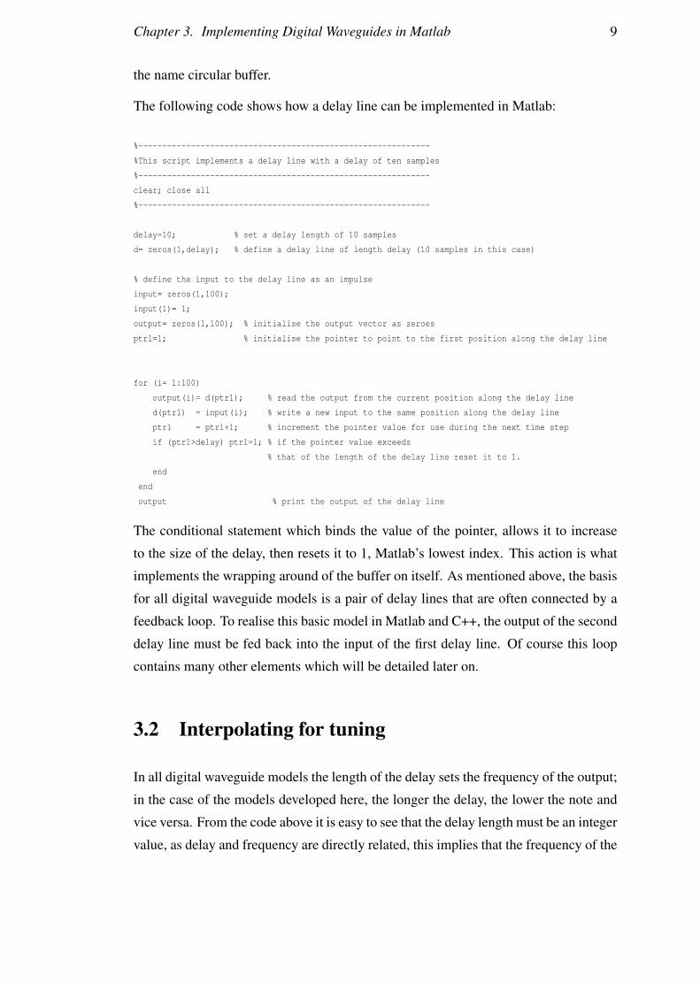


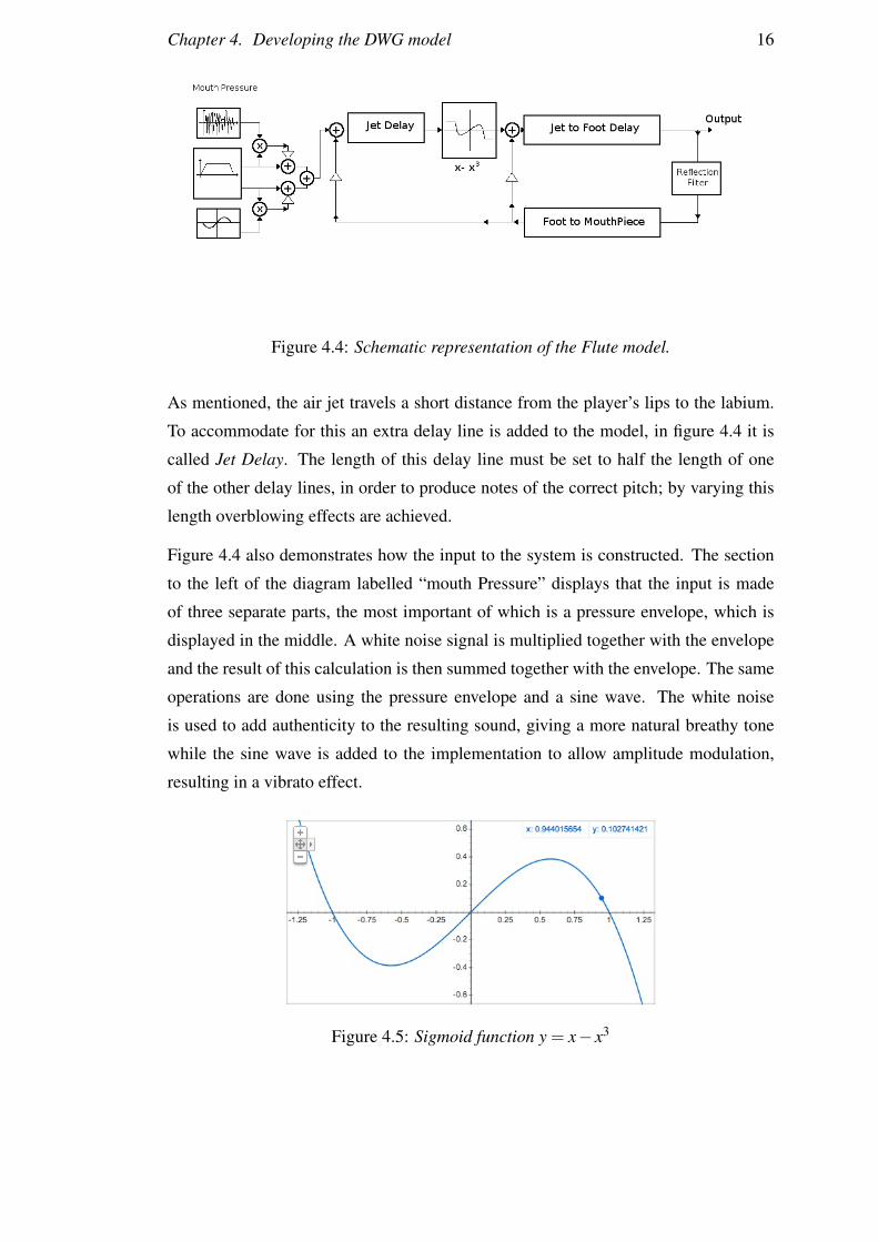


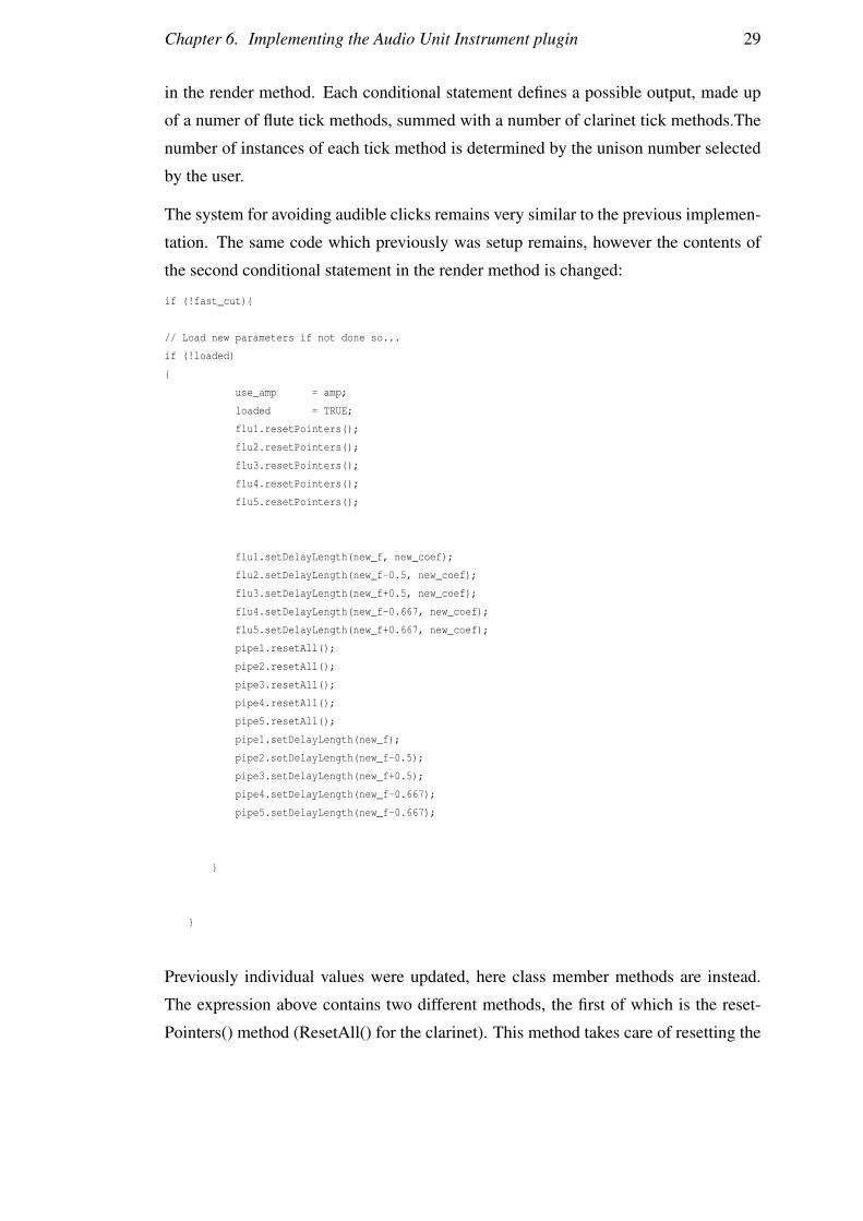

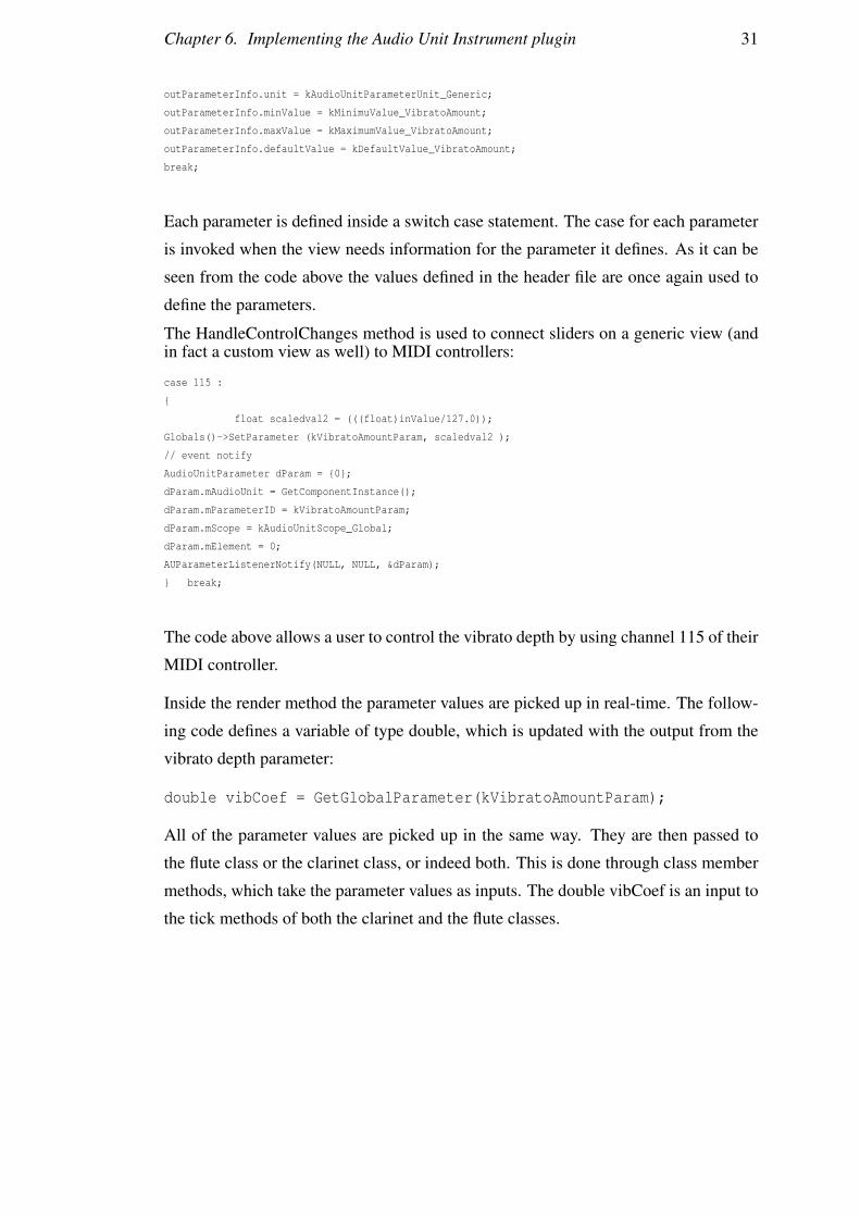


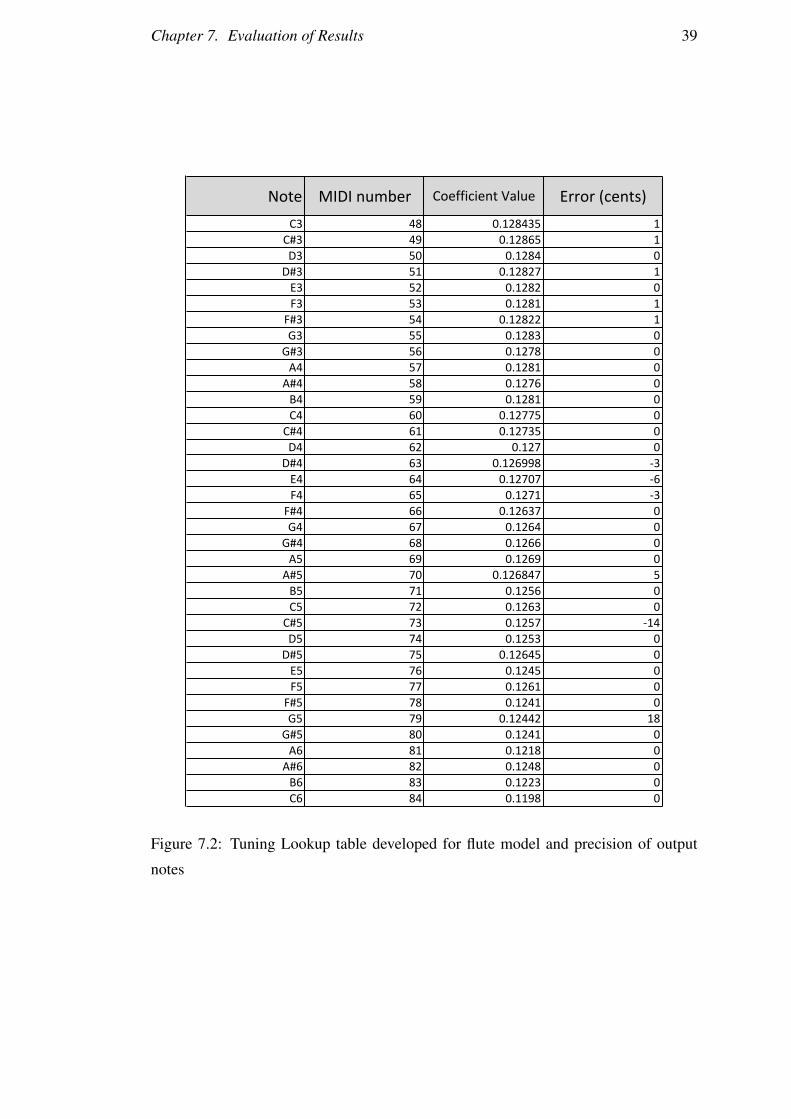


![DIALux4[1].0- · PDF filedialux 2 plugin. 1.X. plugin , plugin. luminaire selection Plugin plugin . home page, Intenet Explorer](https://static.documents.pub/doc/80x56/5a715aac7f8b9a98538cccda/dialux410-wwwpowerengineeringblogfacomssuacirkhadamatkarkonanarticlesbarghdialux4-learningpdfpdf.jpg)


