The Pennsylvania State University
The Graduate School
College of Engineering
DEVELOPMENT AND BENCHMARKING OF IMAGE ANALYSIS
METHODS FOR USE IN HORIZONTAL PLUG FLOW
A Thesis in
Nuclear Engineering
by
Adam Rau
© 2017 Adam Rau
Submitted in Partial Fulfillment
of the Requirements
for the Degree of
Master of Science
May 2017
ii
The thesis of Adam Rau was reviewed and approved* by the following:
Seungjin Kim
Professor of Mechanical and Nuclear Engineering
Thesis Advisor
Justin Watson
Research Associate and Assistant Professor of Nuclear Engineering
Arthur Motta
Professor of Nuclear Engineering
Chair of Nuclear Engineering
*Signatures are on file in the Graduate School.
iii
ABSTRACT
Accurate modeling of two-phase flow in all pipe orientations is important to the
development of best-estimate systems analysis codes, which are used to assess safety margins of
nuclear reactors. These codes use the flow regime approach to supply closure models to the two-
phase flow field equations. The flow regime approach classifies flows into “flow regimes” based
on the shape and structure of the interface between the two phases. In horizontal flow, plug flow
and slug flow are two such flow regimes. Even though significant differences exist between these
regimes, models capturing the differing transport characteristics of plug and slug flow have not
been established.
In view of this, image analysis techniques to measure two-phase parameters of the large,
elongated bubbles that characterize plug flow (plug bubbles) are established in the present work.
Image analysis methods have the ability to characterize the nose of the plug bubbles, which may
be instrumental in studying the differences between plug and slug flow and the transport
characteristics of plug bubbles. A visualization block / mirror system is designed and fabricated to
allow the simultaneous visualization of two-phase flow from the top and side perspectives using a
single camera, and an image processing code is written to measure plug bubble parameters from
high-speed videos of two-phase flow acquired with this system. The code is capable of measuring
the nose position, nose velocity, local time-averaged axial velocity, and time-averaged area-
averaged void fraction of plug bubbles.
Experiments are conducted in the existing horizontal two-phase flow test facility at the
Advanced Multi-Phase Flow Laboratory of the Pennsylvania State University to benchmark the
image analysis technique using the local four-sensor conductivity probe. Agreement within 10%
is observed for the time-averaged area-averaged void fraction measured by the two techniques. For
the local time-averaged axial velocity of plug bubbles, general agreement was observed within
10%. Near the top wall of the pipe, differences as up to 25% were observed.
iv
TABLE OF CONTENTS
LIST OF FIGURES ........................................................................................................................ vi
LIST OF TABLES .......................................................................................................................... ix
ACKNOWLEDGEMENTS ............................................................................................................. x
Chapter 1 Introduction ..................................................................................................................... 1
1.1 Motivation .............................................................................................................................. 1
1.2 Literature Review ................................................................................................................... 3
1.2.1 Horizontal Plug-Slug Flow Regime Transition .............................................................. 3
1.2.2 Two-Phase Flow Image Processing ................................................................................ 6
1.3 Thesis Objectives ................................................................................................................... 9
Chapter 2 Experimental Facility and Instrumentation ................................................................... 10
2.1 Experimental Facility ........................................................................................................... 10
2.1.1 Test Section................................................................................................................... 11
2.1.2 Air / Water Supply System ........................................................................................... 12
2.1.3 Two-Phase Injector ....................................................................................................... 13
2.1.4 Instrumentation Ports .................................................................................................... 13
2.1.5 Visualization Block-Mirror System .............................................................................. 15
2.1.6 Instrumentation ............................................................................................................. 16
2.1.7 Damper / Two-Phase Separator System ....................................................................... 21
2.2 Setup and Alignment Procedures ......................................................................................... 22
2.2.1 Visualization Block-Mirror System Setup .................................................................... 23
2.2.2 Camera Alignment ........................................................................................................ 24
Chapter 3 Development of Image Processing Algorithm .............................................................. 29
3.1 Image Processing Terminology ........................................................................................... 29
3.2 Image Correction ................................................................................................................. 31
3.2.1 Lens Distortion Correction ........................................................................................... 32
3.2.2 Top View Magnification Correction ............................................................................. 34
3.2.3 Cropping ....................................................................................................................... 38
3.2.4 Background Subtraction ............................................................................................... 39
3.3 Gas-Phase Segmentation ...................................................................................................... 41
3.3.1 Thresholding ................................................................................................................. 41
3.3.2 Extraneous Artifact Removal ........................................................................................ 43
3.3.3 Curve Closing ............................................................................................................... 45
3.3.4 Object Filling ................................................................................................................ 55
3.4 Identification and Tracking of Plug Bubbles ....................................................................... 55
3.5 Contacting Bubble Segmentation ......................................................................................... 60
3.5.1 Distance Check ............................................................................................................. 61
3.5.2 Off-screen Collision Procedures ................................................................................... 63
v
3.5.3 Convex Curvature Segmentation Algorithm ................................................................ 75
Chapter 4 Measurement of Two-Phase Parameters and Benchmarking ........................................ 78
4.1 Calibration ............................................................................................................................ 78
4.2 Benchmarking by Local Four-Sensor Conductivity Probe .................................................. 84
Chapter 5 Summary and Recommendations for Future Work ....................................................... 91
References ...................................................................................................................................... 97
Appendix A Dimensional Drawings of Visualization Block / Mirror System ........................... 100
vi
LIST OF FIGURES
Figure 2-1: Schematic of horizontal test facility (from Talley et al., 2015a) ................................. 10
Figure 2-2: Exploded view of instrumentation port (from Talley et al. 2015b)............................. 14
Figure 2-3: Visualization block-mirror system. ............................................................................. 15
Figure 2-4: Illustration of visualization block installation ............................................................. 15
Figure 2-5: Schematic of mating surfaces and pipe surfaces ......................................................... 16
Figure 2-6: Schematic depiction of the local four-sensor conductivity probe (Kim et al., 2000). . 17
Figure 2-7: Measurement mesh used in conductivity probe measurement. ................................... 19
Figure 2-8: (Left) Two Newport Linear Traversing stages are employed to allow fine adjustment
of the camera position in the vertical and the flow directions. (Right) A sliding bearing is employed
to allow coarse adjustment of the camera height. .......................................................................... 20
Figure 2-9: High-speed camera (Photron Fastcam Ultima 512) mounted on the traversing structure.
....................................................................................................................................................... 21
Figure 2-10: Illustration of terms used to refer to visualization block-mirror-camera position and
orientation. ..................................................................................................................................... 23
Figure 2-11: (Left) Support system used to set and maintain level of visualization block. (Right)
Detail of mechanism used to adjust height of the end of each support. ......................................... 24
Figure 2-12: Illustration of principle used to ensure optical axis is normal to front surface of
visualization block. ........................................................................................................................ 25
Figure 2-13: Image acquired to verify alignment of optical axis to the front surface of the
visualization block ......................................................................................................................... 26
Figure 2-14: Geometric parameters used to estimate error in camera squaring procedure. ........... 26
Figure 2-15: Image acquired to verify the camera level about the optical axis and position in the
flow direction. ................................................................................................................................ 28
Figure 3-1: Illustration of pixel adjacency. White pixels are 4-adjacent to center pixel P. Blue and
white pixels are 8-adjacent to pixel P. ........................................................................................... 30
Figure 3-2: Illustration of pixel connectivity. Pixel P is 8-connected to all white pixels shown in
the figure, but is 4-connected only to pixel Q. Unlabeled pixels are mutually connected by either
4- or 8-connectivity. ....................................................................................................................... 31
Figure 3-3: Image correction procedures flow diagram ................................................................. 32
Figure 3-4: Raw two-phase flow image exhibiting lens distortion. Lens distortion makes the front
wall of the pipe (circled) appear to be curved. A straight horizontal line is shown to highlight the
curvature. ....................................................................................................................................... 33
Figure 3-5: Lens distortion correction. (a) Image before lens distortion correction. (b) Image after
lens distortion correction. ............................................................................................................... 34
Figure 3-6: Raw image acquired with visualization block-mirror system, with vertical lines added
to highlight increased optical distance from camera to top view ................................................... 35
Figure 3-7: Illustration of additional path length taken by light traveling from top view. ............ 35
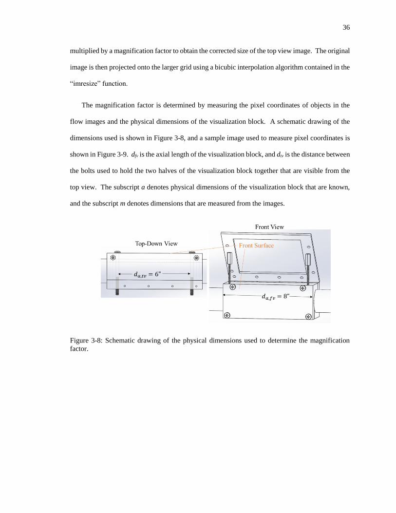
Figure 3-8: Schematic drawing of the physical dimensions used to determine the magnification
factor. ............................................................................................................................................. 36
vii
Figure 3-9: Sample image used to determine magnification factor with measured dimensions
shown. ............................................................................................................................................ 37
Figure 3-10: Two-phase flow image after top view magnification correction and cropping. Vertical
lines are added to show that top view magnification correction has been performed successfully.
....................................................................................................................................................... 38
Figure 3-11: Image after top-view magnification correction and cropping ................................... 39
Figure 3-12: Input and output of background subtraction procedure ............................................ 40
Figure 3-13: Image after thresholding ........................................................................................... 42
Figure 3-14: Illustration of gas-phase regions not detected by thresholding procedure. ............... 43
Figure 3-15: Thresholded image of plug flow. Regions incorrectly assigned to gas-phase are
circled. ............................................................................................................................................ 44
Figure 3-16: Image of two-phase flow superimposed on the background image. The plug bubble
is causing brightness variations in the pipe wall (right circled area). The same brightness variation
is not present downstream of the plug bubble (left circled area). .................................................. 44
Figure 3-17: Image after extraneous artifact removal. ................................................................... 45
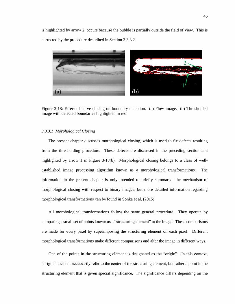
Figure 3-18: Effect of curve closing on boundary detection. (a) Flow image. (b) Thresholded
image with detected boundaries highlighted in red. ...................................................................... 46
Figure 3-19: Illustration of dilation transformation. ...................................................................... 48
Figure 3-20: Illustration of erosion transformation. ....................................................................... 49
Figure 3-21: Illustration of morphological closing procedure ....................................................... 50
Figure 3-22: Illustration of "boundary complete" algorithm ......................................................... 53
Figure 3-23: Example of a case where a bubble in contact with the plug bubble induces a sudden
change in the minimum y-coordinate. The detected interface is highlighted in red, and the minimum
y-coordinates are highlighted in blue. ............................................................................................ 54
Figure 3-24: Example of improvement in interface detection from curvature closing techniques.
(a) Interface detected before curve closing. (b) Interface detected after curve closing. ............... 54
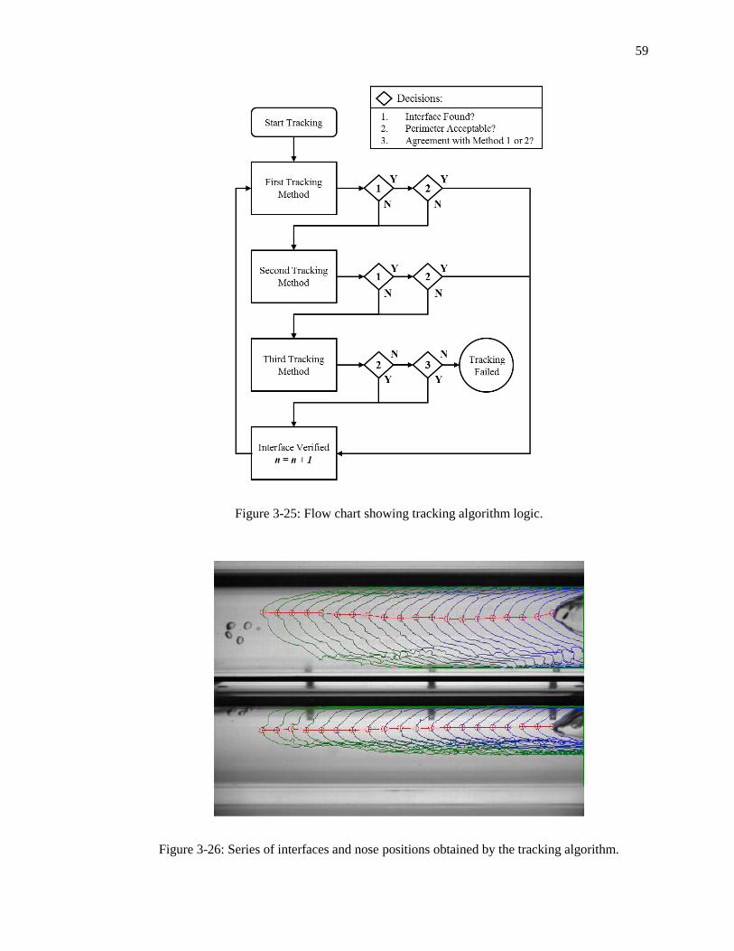
Figure 3-25: Flow chart showing tracking algorithm logic. .......................................................... 59
Figure 3-26: Series of interfaces and nose positions obtained by the tracking algorithm. ............ 59
Figure 3-27: Example of a small bubble contacting the plug bubble ............................................ 61
Figure 3-28: Change in detected interface as plug bubble overtakes dispersed bubble cluster
(detected interface highlighted in blue). ........................................................................................ 62
Figure 3-29: Dispersed bubble entrained by plug bubble without coalescing ............................... 64
Figure 3-30: Illustration of adaptive threshold principle ............................................................... 65
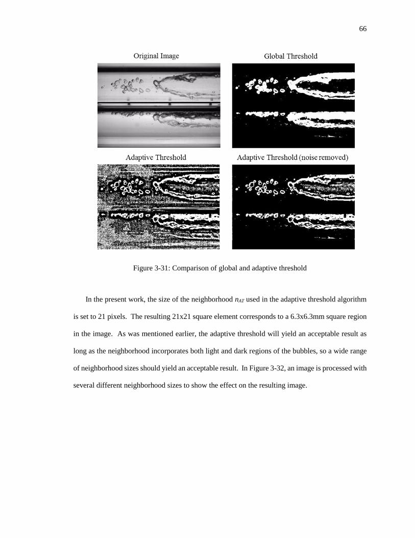
Figure 3-31: Comparison of global and adaptive threshold ........................................................... 66
Figure 3-32: Comparison of results of adaptive threshold algorithm with different neighborhood
sizes ................................................................................................................................................ 67
Figure 3-33: Result of modified "MB2" thinning algorithm with original image superimposed .. 68
Figure 3-34: Illustration of benefit of using parallel closing element sizes. Some erroneous
breakpoints will only be detected in the 3x3 closed image (circled in red), and other will only be
detected in the 5x5 closing element image (circled in blue). ......................................................... 68
Figure 3-35: Scaled depiction of total internal refraction for a spherical air bubble in water ....... 70
viii
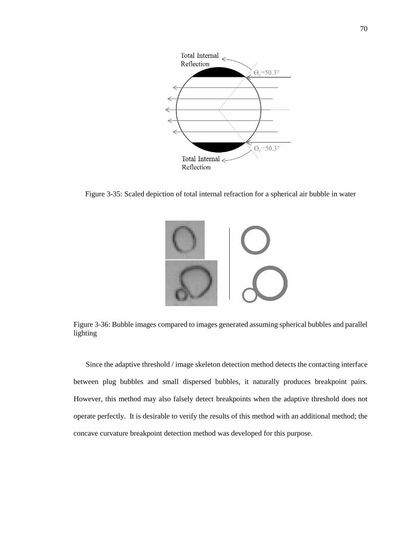
Figure 3-36: Bubble images compared to images generated assuming spherical bubbles and parallel
lighting ........................................................................................................................................... 70
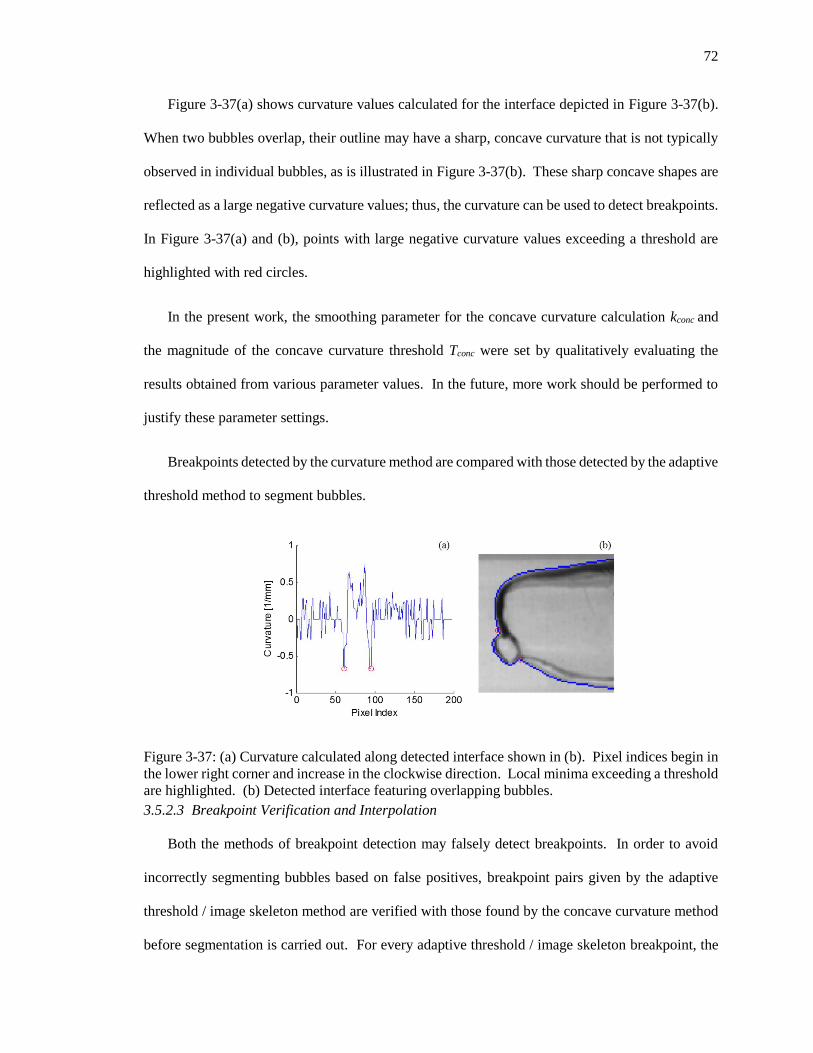
Figure 3-37: (a) Curvature calculated along detected interface shown in (b). Pixel indices begin in
the lower right corner and increase in the clockwise direction. Local minima exceeding a threshold
are highlighted. (b) Detected interface featuring overlapping bubbles. ........................................ 72
Figure 3-38: Example interface produced by contacting bubble segmentation. Interface is
highlighted in red. .......................................................................................................................... 77
Figure 4-1: Schematic description of pinhole camera (from Jähne, 1997). Apparent positions of
objects are related to the angle of the ray entering the camera. ..................................................... 79
Figure 4-2: Differing true and apparent position caused by refraction .......................................... 79
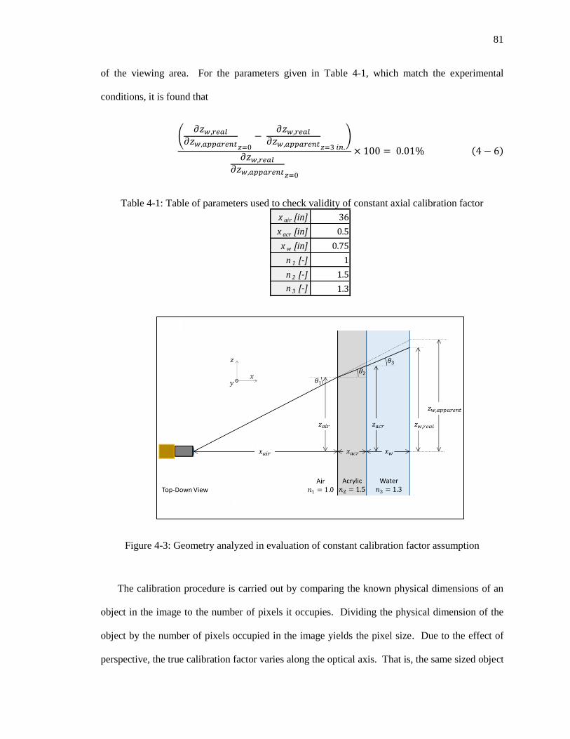
Figure 4-3: Geometry analyzed in evaluation of constant calibration factor assumption .............. 81
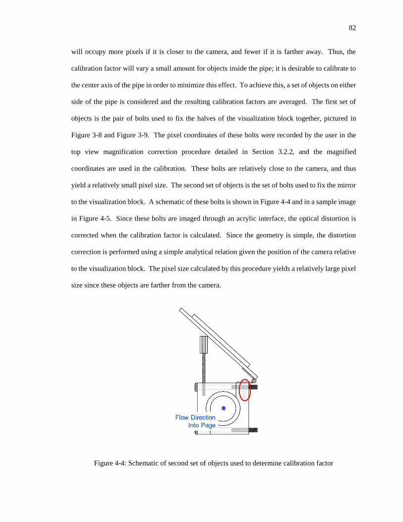
Figure 4-4: Schematic of second set of objects used to determine calibration factor .................... 82
Figure 4-5: Second set of bolts used in axial calibration ............................................................... 83
Figure 4-6: Flow conditions for benchmarking experiments shown on flow regime map of Kong
and Kim (2017). ............................................................................................................................. 84
Figure 4-7: Benchmark of local time-averaged axial velocity of plug bubbles for jf=1.00 m/s and
jg=0.33 m/s ..................................................................................................................................... 87
Figure 4-8: Benchmark of local time-averaged axial velocity of plug bubbles for jf=1.00 m/s and
jg=0.15 m/s ..................................................................................................................................... 87
Figure 4-9: Illustration of bubble reconstruction procedure. (a) Coordinates of the boundaries
enclosing the cross-section are found for a given axial position. (b) Ellipse shape is fit within the
boundaries defined in (a) ............................................................................................................... 89
ix
LIST OF TABLES
Table 2-1: Typical geometric parameters for camera alignment and associated error in alignment
of optical axis to visualization block.............................................................................................. 26
Table 4-1: Table of parameters used to check validity of constant axial calibration factor .......... 81
Table 4-2: Sample sizes for the current measurements .................................................................. 85
Table 4-3: Area-averaged time-averaged void fraction benchmark............................................... 90
Table 4-4: Total area-averaged time-averaged void fraction measured by the probe compared to
void fraction of plug bubbles measured by image analysis ........................................................... 90
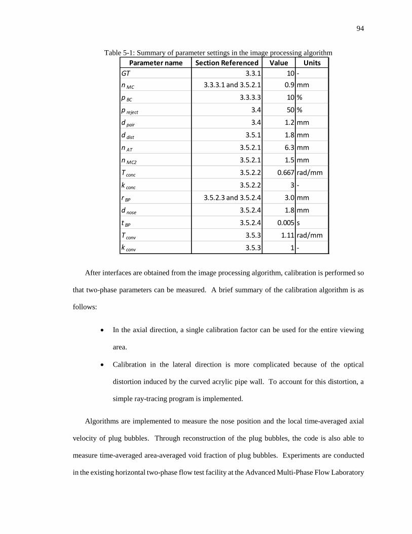
Table 5-1: Summary of parameter settings in the image processing algorithm ............................. 94
x
ACKNOWLEDGEMENTS
The author would like to express his sincere gratitude to his thesis advisor, Dr. Seungjin Kim.
Dr. Kim is extraordinarily committed to the growth of each of his students and to the advancement
of two-phase flow research. The author is indebted to Dr. Kim for his mentorship, which has made
this work a journey of continuous self-improvement.
The author would also like to thank the members of the thesis committee for reviewing the
document and providing valuable feedback. Thanks are also due to the United States Nuclear
Regulatory Commission for supporting the author through the NRC Fellowship Program.
The author would also like to express his appreciation to his colleagues at the Advanced Multi-
Phase Flow Laboratory. Particular thanks are due to Dr. Ted Worosz, Mr. Shouxu Qiao, and Mr.
Ran Kong, for providing the author with invaluable advice and guidance at various stages of his
graduate study. The author feels fortunate to have worked with each of them and has enjoyed his
time doing so.
Finally, the author would like to thank his parents, Jay and Michelle, and his brother Ethan, for
their continued support and encouragement throughout the present work. The author would also
like to thank his girlfriend, Maxine Fox, for her continued love and daily support.
Chapter 1
Introduction
1.1 Motivation
Modeling two-phase flow in pipes is a topic of great importance to a variety of industries,
including the oil and gas and the nuclear power industry. In the nuclear power industry, accurate
modeling of two-phase flow in all pipe orientations is important to the development of best-estimate
systems analysis codes, which are used to assess reactor safety margins. These systems analysis
codes use the flow regime approach to supply closure models to the two-phase field equations. The
flow regime approach classifies flows into “flow regimes” based on the shape and structure of the
interface between the two phases. Flow regimes can be dependent on liquid and gas flow rates,
fluid properties, pipe orientation with respect to gravity, and pipe size. Previous researchers have
established “flow regime maps” that specify a flow regime based on given flow rates of liquid and
gas. Constitutive relations are then specified for the given flow regime.
For horizontal two-phase flow, six commonly defined flow regimes are “bubbly flow” (also
called “dispersed flow” or “dispersed bubbly flow”), “plug flow”, “slug flow”, “annular flow”,
“stratified flow”, and “stratified-wavy flow” (Kong and Kim, 2017). The plug flow regime, which
is the focus of the present work, and the slug flow regime are both characterized by the alternating
appearance of long bubbles that occupy the upper portion of the pipe and liquid regions that may
contain small dispersed bubbles. Although some previous researchers have combined plug and
slug flow into a single regime (typically called “intermittent flow”), important differences exist
between the regimes. For example, the population of small dispersed bubbles in the liquid region
can be much higher in slug flow than in plug flow. This can lead to higher concentration of
interfacial area (as demonstrated by the data of Kong et al., 2016), an important parameter that
affects the rate of heat and mass transfer between the gas and liquid phases. The alternating
2
appearance of gas and liquid regions also causes pressure fluctuations in slug flow that are much
less marked in plug flow (Ruder and Hanratty, 1990). The shape of the large elongated bubbles in
these flow regimes can also be different. Some researchers (Fagundes Netto et al. 1999, Talley
2012, Kong and Kim 2017) have noted the presence of long thin tails at the rear of the plug bubbles
which are absent from slug bubbles. Observation of high-speed flow visualizations of the two
regimes reveals differences in the character of the nose of the plug / slug bubbles. Furthermore,
although models have been proposed to predict the internal structure of slug flow (Dukler and
Hubbard, 1975), these models are based around modeling of the liquid slug. Liquid slugs are not
typically included in the description of plug flow and may not be a fundamental part of the flow
structure.
Because of these differences, it is important to understand the mechanism for transition
between these two flow regimes, yet relatively little work has been performed to model this
transition in comparison to other flow regime transitions in horizontal flow. Previous researchers
have observed differences in the nose position and nose shape between plug and slug flow (de
Oliviera et al., 2015; Fagundes Netto et al., 1999). In the present work, it is posited that the flow
regime transition and plug bubble transport are related to the characteristics of the plug / slug bubble
nose. While the local four-sensor conductivity probe is available for two-phase flow
measurements, this technique may not be able to measure the characteristic features of the plug
bubble nose. This instrument is capable of measuring local time-averaged two-phase parameters
throughout the pipe cross-section. However, because the nose position changes continuously,
characteristics of the plug bubble nose may not be reflected by these data. In contrast, image
analysis methods are able to resolve the interface of plug bubbles at a given instant, and so this
method can measure the nose parameters directly. In view of this, an image processing code
capable of analyzing the shape and motion of plug bubbles is developed in the present work.
3
1.2 Literature Review
1.2.1 Horizontal Plug-Slug Flow Regime Transition
Early horizontal flow regime maps were published by a variety of researchers based on
relatively small experimental databases. Govier and Aziz (1972) developed a flow regime map for
horizontal air-water flow incorporating the work of several previous researchers. They used
measurements of the slip ratio to draw the transition line between plug and slug flow as well as the
line between stratified and stratified-wavy flow. Specifically, they observed that the slip ratio
generally increases with increasing superficial gas velocity, but decreases over a small band of
superficial gas velocities. They proposed a regime transition line from plug/stratified flow to
slug/stratified-wavy flow within this small band of superficial velocities, arguing that the slip
decreases because the interface becomes rougher, increasing the interfacial drag and lowering the
gas velocity. Later Mandhane et al. (1974) revised the map proposed by Govier and Aziz (1972)
in order to produce a better fit with the available data. They compared their map to a two-phase
flow database compiled by the American Gas Association and American Petroleum Institute, which
contained approximately 1,000 data points for horizontal air-water two-phase flow. It is important
to note that most of the air-water data used by Mandhane et al. (1974) was obtained from 13-50
mm pipes. The maps of Govier and Aziz (1972) and Mandhane et al. (1974) are largely similar
even though the latter was formulated using a more extensive database. Among the differences
between the maps, the transition line from plug to slug flow and from stratified to stratified-wavy
flow was moved to a higher superficial gas velocity, although both lines demonstrate the same
trend.
Taitel and Dukler (1976) developed theoretical models for all flow regime transitions and a
resulting flow regime map. They did not distinguish between plug and slug flow, but rather grouped
these flow regimes into a single “intermittent” flow regime. They observed good general agreement
4
with Mandhane et al. (1974), but noted a significant effect of pipe size on the flow regime transition
boundaries, even for the range of diameters reported in the study by Mandhane et al. (1974).
Weisman et al. (1979) performed flow regime identification studies using flow visualization.
They defined plug flow by the presence of large elongated bubbles traveling over a liquid layer,
and characterized slug flow by the “packets of liquid (slugs) that periodically move down the tube.”,
although they did not specify how these flow regimes were differentiated from each other in the
visualization study. They also measured time traces of pressure to mitigate subjectivity in the flow
regime identification. In the pressure measurement, they differentiated slug flow from other flow
regimes by the presence of large pressure peaks followed by long quiescent regions, and plug flow
by pressure oscillations that occurred under a certain frequency. They also designated a sub-regime
between plug flow and dispersed bubbly flow which they called bubble flow , characterized as
having bubbles that are on top of the pipe instead of dispersed throughout the pipe. This occurs at
low gas flow rates and high liquid flow rates between plug flow and dispersed bubbly flow.
Barnea and Brauner (1985) established a model to predict void fraction inside the liquid slug
based on the assumption that the liquid slug will accommodate the same void fraction as a condition
on the intermittent/bubbly transition with the same mixture velocity. They argued that for a given
turbulence level, there is an upper limit on the amount of void that can exist as dispersed bubbles
before coalescence occurs. As the flow transitions to plug or slug flow, any void beyond this
maximum limit coalesces to form plug/slug bubbles, and the rest remains dispersed throughout the
liquid slugs. Therefore, the void fraction in the liquid slug will be the same as that of a condition
on the intermittent/bubbly transition line with the same level of turbulence. They approximated by
the turbulence level in the flow by the mixture velocity. They also suggested that plug flow is a
limiting case of slug flow where there is no aeration in the liquid slug, and developed a plug/slug
transition line based on their model for void fraction in the liquid slug.
5
Ruder and Hanratty (1990) performed flow visualization studies and pressure pulsation
measurements with the goal of finding a transition boundary between horizontal plug and slug flow.
They attempted to use pressure pulsation measurement, which had been implemented for flow
regime identification by previous researchers. While they did observe a decreasing magnitude of
pressure fluctuation in the transition from slug flow to plug flow, they did not observe a sharp
change in fluctuation magnitude that could be used to identify a flow regime transition with this
method. Instead, Ruder and Hanratty (1990) proposed two potential flow regime transition criteria
based on the shape of the rear of the plug bubble. The first was that transition occurs when a
“staircase” type structure of the tail is exhibited, where the liquid level under a plug bubble
suddenly jumps from a near constant level to a higher near constant level. Other researchers have
observed this structure at lower superficial gas velocities (Talley et al., 2015a), but not at higher
superficial gas velocities. The second potential criteria was that transition occurs when the bubble
appears to be symmetric, in that the rear of the bubble is shaped like the front of the bubble. Ruder
and Hanratty (1990) likened this shape to that predicted by Benjamin (1968), sometimes called the
“Benjamin bubble”. They noted that transition criteria based on bubble shape were generally
advantageous because they can be associated with changes in hydrodynamics, which can be
modeled mathematically.
Fagundes Netto et al. (1999) measured bubble velocity, shape and length using vertical wire
probes and developed a model for bubble shape. They divided the bubble into nose, body, hydraulic
jump and tail regions, where the hydraulic jump and tail regions refer to the “staircase” structure
observed by Ruder and Hanratty (1990). The bubble shape model is then able to predict whether a
bubble will possess a tail based on the flow conditions and the bubble length. Fagundes Netto et
al. (1999) then predicted the transition between plug and slug flows based on whether or not the
large, elongated bubbles possess tails. Using measured bubble lengths, they also predicted a
transition region where shorter bubbles will have tails and longer bubbles will not.
6
Talley et al. (2015a) performed a flow visualization study in a 38 mm inner diameter air-water
horizontal flow facility to investigate interfacial structures in relation to flow regime transition. He
observed two mechanisms by which small dispersed bubbles can be generated from plug bubbles,
spurring the transition to slug flow. First, he observed that waves in the plug bubble tails can cause
them to break away from the plug bubble when waves bridge the pipe. However, Talley argued
that this phenomenon alone cannot account for the large populations of plug bubbles observed in
slug flow. He also observed shearing off of small bubbles from the body of the plug bubbles due
to the relative velocity between the liquid film and the gas plug/slug.
De Oliveira et al. (2015) employed image processing techniques to quantify bubble shape as a
means of accessing transition from plug to slug flow. Following the work of Fagundes Netto et al.
(1999), they measured the angle of inclination of the “staircase” structure of the large elongated
bubbles. While they did observe that the angle of this structure became larger (or the “staircase”
portion on the bubble became steeper), the change in angle was within the experimental error of
the code and could not be used to define a flow regime transition.
Kong and Kim (2017) performed a comprehensive flow regime identification study using flow
visualizations obtained with a high-speed video camera. They characterized plug flow as having
thin elongated tails, similar to those described by Ruder and Hanratty (1990). They also observed
rotating bubble clusters on the order of the gas slug depth as described by Dukler and Hubbard
(1975) were present in slug flow, but not in plug flow. They developed a flow regime map for air-
water flow through a 38 mm ID acrylic pipe.
1.2.2 Two-Phase Flow Image Processing
Image processing encompasses a broad and varied class of techniques that have been
implemented in a wide variety of applications. Among two-phase flow instrumentation techniques,
image processing has the advantage of being non-intrusive, meaning that measurement will not
disturb the flow field. In addition, recent advancements in high-speed movie camera technology
7
enable image processing measurements to achieve high spatial and temporal measurement
resolutions (Fu and Liu, 2016). For these reasons, many previous researchers have used image
processing in order to study the hydrodynamics of two-phase flow; the current section is intended
to give a brief overview of previous work conducted to this end.
Some of the earliest image processing techniques involved manual processing of photograph
sequences. For example, Davies and Taylor (1950) used sequences of photographs to quantify the
rise velocity and shape of large air bubbles in water. However, automated algorithms are of interest
for their ability to process large amounts of data in a short time period, and have been in
development for some time. As early as 1981, Schrodt and Saunders (1981) demonstrated an image
analysis system for measurement of gas bubble size in a gas-liquid reaction system, using edge
detection techniques to detect gas-liquid interfaces. Similar image processing techniques for
detecting outlines bubbles have been implemented by various researchers (Polonsky et al., 1999;
Nogueira et al., 2003; Mayor et al., 2007) to study the shape and motion of slug bubbles in vertical
upward two-phase flow.
More recently, de Oliviera et al. (2015) applied image processing techniques to study horizontal
air-water plug and slug flow in a 50.8 mm pipe. Rather than capturing high-speed images of plug
and slug flow, they captured bursts of photographs by synchronizing a camera with a mechanism
for detecting slug bubbles. They also used matched index of refraction techniques to reduce optical
distortion at the interface of the pipe. Rattner and Garimella (2015) applied image processing
techniques to study vertical upward slug flow in 6.0-9.5 mm round tubes. They developed an
algorithm to correct for vibration or movement of their camera automatically. They also created
simulated images of their experimental setup using ray-tracing software in order to validate their
calibration approach and to evaluate the potential for optical distortion due to refraction effects in
their system. Fu and Liu (2016) developed a novel image processing technique to study vertical
upward bubbly flow. Their technique is capable of separating and reconstructing interfaces of
8
overlapping bubbles. Implementation on artificially generated images suggests that the algorithm
can accurately measure bubble number density at void fractions up to 18%. Rau et al. (2016)
developed image processing techniques for plug bubbles in horizontal flow and performed
preliminary benchmarking with the local four-sensor conductivity probe.
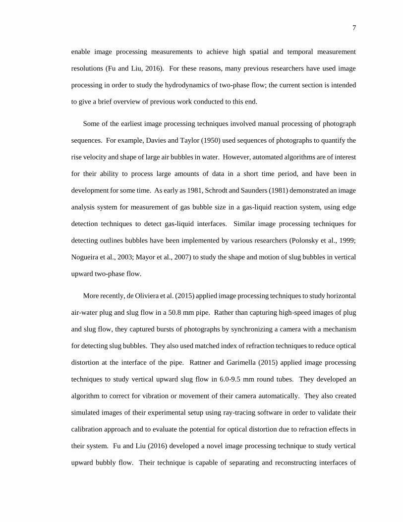
As the literature review reveals, while previous researchers have proposed both models and
empirical correlations for transition between the plug flow regime and the slug flow regime, a
regime transition model that addresses the differences in transport characteristics between plug and
slug bubbles has not been proposed. To aid in the development and validation of such a model, an
experimental database of the characteristics of plug bubble features, such as the nose, should be
established. In view of this, an image processing code capable of analyzing the shape and motion
of plug bubbles is developed in the present work.
9
1.3 Thesis Objectives
In view of the literature survey and the significance of the current work, the objectives of this
thesis are to:
1) Design and fabricate a system to allow simultaneous visualization of the top and side views
of the flow
2) Develop an automated image processing algorithm capable of measuring shape and
velocity of plug bubbles
3) Benchmark said image processing algorithm using the local four-sensor conductivity probe
4) Establish an experimental database of plug bubble velocity and shape information
10
Chapter 2
Experimental Facility and Instrumentation
2.1 Experimental Facility
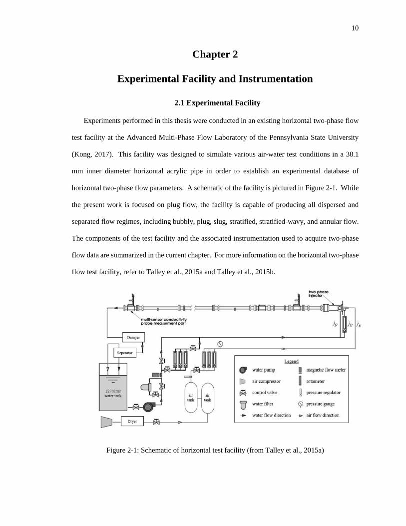
Experiments performed in this thesis were conducted in an existing horizontal two-phase flow
test facility at the Advanced Multi-Phase Flow Laboratory of the Pennsylvania State University
(Kong, 2017). This facility was designed to simulate various air-water test conditions in a 38.1
mm inner diameter horizontal acrylic pipe in order to establish an experimental database of
horizontal two-phase flow parameters. A schematic of the facility is pictured in Figure 2-1. While
the present work is focused on plug flow, the facility is capable of producing all dispersed and
separated flow regimes, including bubbly, plug, slug, stratified, stratified-wavy, and annular flow.
The components of the test facility and the associated instrumentation used to acquire two-phase
flow data are summarized in the current chapter. For more information on the horizontal two-phase
flow test facility, refer to Talley et al., 2015a and Talley et al., 2015b.
Figure 2-1: Schematic of horizontal test facility (from Talley et al., 2015a)
11
2.1.1 Test Section
The horizontal facility test section consists of 38.1 mm inner diameter acrylic pipes, and is 9.45
m (or 248 pipe diameters) long. The facility length and diameter were selected to provide adequate
development length for the horizontal two-phase flow while ensuring rigidity of the test section for
the desired flow conditions. Because bubbles will continuously expand as pressure drops along the
pipe length, two-phase flow never reaches a fully developed condition. However, the flow will
reach a ‘quasi-developed’ state when bubble interaction mechanisms offset expansion to create a
relatively stable flow configuration. Since the buoyancy force acts perpendicular to the flow
direction in horizontal flow, stable flow patterns will, for the conditions considered in the present
work, require bubbles to rise to the top of the pipe. In general, the rise velocity of bubbles can be
significantly less than their axial velocity, which can result in long development lengths for
horizontal two-phase flow. Therefore, the test section was built to the maximum length allowed
by the laboratory space.
The facility is constructed out of multiple clear acrylic horizontal pipes connected in series.
The pipes are connected through acrylic flanges and are aligned using dowel pins. Because of the
variations in the pipe diameter that result from the manufacturing process, the ends of the pipes are
tapered at a maximum angle of 3° over a length of 10 mm to the same diameter at each end. After
tapering, the ends of the pipes are sanded and polished to match the manufactured surface condition.
The test section is supported through a series of acrylic support blocks connected to a rigid
steel structure. Rubber pads are installed between the test section and support blocks to cushion
the pipes and damp vibrations. Vertical alignment of the test section is achieved using shim stock
and verified with a digital level with an accuracy of ±1%. Horizontal alignment is achieved using
a laser beam referenced to a fixed position relative to the dowel pins.
12
2.1.2 Air / Water Supply System
In order to simulate all possible horizontal flow patterns, the facility must be able to supply
adequate air and water flow. To supply air to the facility, a 30 HP Quincy QGV30 rotary screw air
compressor is employed. The compressor has a capacity of 137.9 ACFM at the set point of 689
kPa (100 psig). After the air leaves the compressor, it passes through an in-line filter, a dryer, and
an additional in-line filter. This removes moisture from the air as well as oil that may have been
entrained from the compressor. The compressed air is stored in three accumulator tanks connected
in series. The three tanks have volumes of 0.97 m3, 1.51 m3, and 0.45 m3. These tanks are employed
to reduce pressure fluctuations in the air supply. In addition, an inline particulate filter is placed
between the most upstream tank and the later two tanks. The air is regulated to a pressure of 414
kPa (60 psig) before entering the rotameter bank, where the volume flow rate of air is measured.
The facility water is supplied with a 60 HP Dean Model pH-2140 pump with a 0.22 m impeller.
The pump is controlled by an AC Tech MCH series variable frequency drive, which allows the user
to control the liquid flow rate by adjusting the pump frequency. A 2.27 m3 accumulator tank
provides water to the pump. This tank is mounted above the pump, and liquid level is maintained
to provide adequate net positive suction head to the pump to prevent cavitation.
The facility water is treated with a Siemens Water Technologies filtration system in order to
ensure high-quality water is used in the experiments. The system includes a carbon filter, which
removes particulates and organic compounds, and two mixed resin bed filters, which remove ions
from the water. The deionized water is then treated with morpholine and ammonium hydroxide.
Ammonium hydroxide is used to maintain the facility water at a pH of approximately 10.
Morpholine is added to reduce corrosion of the pump and to maintain the water conductivity at
approximately 100 μS/cm so that the conductivity probe and magnetic flow meter can be used.
13
2.1.3 Two-Phase Injector
Two-phase flow is introduced to the test section at the two-phase injector. A double annulus
geometry was selected for the injector in order to ensure that a constant bubble size is generated
for all test conditions. The main liquid flow is injected to the outer annulus through three 51 mm
diameter lines located at the injector sides and bottom. This line size was selected to ensure that
adequate liquid flow can be supplied to the facility, and the injection lines were configured around
the outside of the annulus in order to reduce swirl. To reduce swirl further, a stainless steel
honeycomb-style flow straightener with a length of 76 mm is installed at the outer annulus just
upstream of the mixing region. A tap is also included at the injector top to allow the removal of
trapped air during facility start up so that unmetered air is not introduced into the test section.
Air is injected through a 25 mm outer diameter stainless steel sparger located at the center of
the inner annulus. The sparger has a porous section with an average pore size of 10 micrometers
and a surface area of 81.1 cm2. An auxiliary liquid flow is supplied to the inner annulus to shear
bubbles from the sparger. This auxiliary flow rate is kept constant for all experimental conditions,
ensuring a consistent bubble size is injected for all test conditions. Seven pipe diameters are
provided between the auxiliary liquid flow injection and the porous region of the sparger. A
reducing section is installed at the end of the injector, which reduces the flow area from that of the
outer annulus to that of the test section. The angle of the reducing section is 23° in order to avoid
the generation of recirculation regions.
2.1.4 Instrumentation Ports
Five instrumentation ports are installed along the axial length of the facility. These ports are
designed to allow for high-speed flow visualization, local four-sensor conductivity probe
measurement, and pressure measurement. The body of the instrumentation port is an acrylic
cylinder with a hole the size of the inner pipe diameter machined into the middle. Two faces of the
cylinder are shaved flat; one to reduce optical distortion for the purpose of flow visualization, and
14
the other to allow for the installation of conductivity probes and impulse lines for pressure
measurement. A linear traverse that is used to set the radial position of the conductivity probe
within the pipe. The port attaches to the facility through an acrylic bearing on either side, which
allows the port to be rotated without stopping the flow. This enables the azimuthal angle coordinate
of the probe to be changed, allowing the entire cross-section of the flow to be measured without
stopping the flow. This is particularly important in the horizontal configuration because the two-
phase flow can be highly asymmetric. Thus, measurement throughout the entire pipe cross-section
is required to accurately assess area-averaged parameters and observe local behavior. For each
port, one rotating flange features a locking mechanism that allows the azimuthal coordinate of the
probe to be set every 22.5°.
Figure 2-2: Exploded view of instrumentation port (from Talley et al. 2015b)
15
2.1.5 Visualization Block-Mirror System
A visualization block-mirror system is designed and fabricated to allow the simultaneous
visualization of the top and side views of the flow from a single camera. Photographs of the
fabricated system are shown in Figure 2-3. The visualization block is similar in design to the
visualization block described in Talley et al. (2015a). Because the curved outer surface of the pipe
can distort the images of the flow, the block is fabricated with flat viewing surface on the top and
side. Some distortion is still present in the images due to the refraction of light through the acrylic
block and pipe wall, but this is compensated for in the image processing algorithm, detailed in
Section 4.1. The block is fabricated in two halves, which mate together and fit around the outside
of the test section. This design allows the system to be installed at different development lengths.
An illustration of this is shown in Figure 2-4.
Figure 2-3: Visualization block-mirror system.
Figure 2-4: Illustration of visualization block installation
16
The mating surfaces of the visualization block are positioned so that they do not obstruct the
top view of the flow, which is pictured in Figure 2-5. Point A is vertically aligned with the inner
surface of the pipe so the associated mating surface does not obstruct the top view of the flow.
Point B is located 180° away from point A so that the two halves of the block can be assembled
around the outside of the pipe. Due to the placement of point B, the bottom 6% of the side view is
obstructed by the associated mating surface. However, it is anticipated that little gas-phase will
occupy this portion of the pipe in horizontal plug and slug flow.
Figure 2-5: Schematic of mating surfaces and pipe surfaces
2.1.6 Instrumentation
The facility is equipped with rotameters and a magnetic flow meter to measure the flow rates
of air and water into the facility. A Yamatake MagneW Two-wire PLUS electromagnetic flow
meter (MTG18B) with an accuracy of ±0.5% is employed to measure water flow rates greater than
1 m/s. Because this flow meter is less sensitive at lower flow rates, a group of rotameters each with
an accuracy of ±2% is employed for lower liquid flow rate conditions. A group of rotameters is
also employed to measure air flow rates, each with an accuracy of ±3%.
17
Pressure is measured using a Yamatake ST3000 series differential pressure transducer. The
differential pressure between any two instrumentation ports can be measured, or the local gauge
pressure can be measured by leaving one of the transducer’s impulse line connections open to
atmosphere. This transducer has an accuracy of ±0.5% between 0.75 kPa and 5 kPa, and an
accuracy of ±0.1% between 5 kPa and 50 kPa.
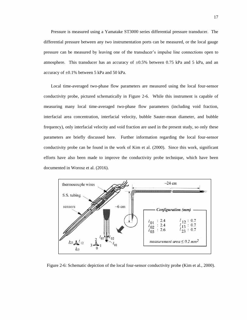
Local time-averaged two-phase flow parameters are measured using the local four-sensor
conductivity probe, pictured schematically in Figure 2-6. While this instrument is capable of
measuring many local time-averaged two-phase flow parameters (including void fraction,
interfacial area concentration, interfacial velocity, bubble Sauter-mean diameter, and bubble
frequency), only interfacial velocity and void fraction are used in the present study, so only these
parameters are briefly discussed here. Further information regarding the local four-sensor
conductivity probe can be found in the work of Kim et al. (2000). Since this work, significant
efforts have also been made to improve the conductivity probe technique, which have been
documented in Worosz et al. (2016).
Figure 2-6: Schematic depiction of the local four-sensor conductivity probe (Kim et al., 2000).
18
The local four-sensor conductivity probe uses the conductivity difference between the gas and
liquid phases to measure local two-phase parameters. The probe operates by creating an electrical
circuit between the sensor tips and probe body using the continuous liquid-phase. The circuit is
complete when a sensor tip is immersed in the liquid-phase, but when a sensor tip is in the gas-
phase the circuit is broken. Thus, the voltage measured from the sensors varies as a near step
function, having a higher value when the sensor resides in gas and a lower value when the sensor
resides in liquid. Local time-averaged void fraction α can be measured by dividing the gas-phase
residence time tgas by the total measurement time ttotal:
𝛼 =𝑡𝑔𝑎𝑠
𝑡𝑡𝑜𝑡𝑎𝑙
(2 − 1)
As shown in Figure 2-6, one sensor is located upstream of the other three. Signals from the
upstream sensors are paired with those of the three downstream sensors to obtain three
measurements of interfacial velocity:
𝑣𝑖,𝑛 =Δ𝑠𝑛
𝑡𝑑𝑒𝑙𝑎𝑦,𝑛
(2 − 2)
where vi,n is the nth measurement of interfacial velocity, Δ𝑠𝑛 is the separation distance between
the sensors and 𝑡𝑑𝑒𝑙𝑎𝑦,𝑛 is the time delay between successive bubble detection by the upstream
sensor and the nth downstream sensor.
Local time-averaged data can be acquired throughout the pipe cross-section using the
instrumentation port described in Section 2.1.4. The measurement mesh used to acquire local data
in the present work is shown in Figure 2-7.
19
Figure 2-7: Measurement mesh used in conductivity probe measurement.
A Photron Fastcam Ultima 512 camera is employed to capture high-speed videos for use with
the image analysis program. The Photron Fastcam Ultima 512 is capable of capturing video at
2000 frames per second at the full 512 x 512 resolution, and is capable of capturing video at up to
32,000 frames per second at reduced resolutions. Photron Fastcam Viewer (PFV) version 3.600
software is employed to operate the camera. This software allows for independent adjustment of
the camera’s frame rate, shutter speed, and resolution. The software also allows for measurement
and display of pixel coordinates on the live or captured image, which is used in the alignment and
positioning of the camera.
A Computar C-Mount 12.5-75mm varifocal lens (model number M6Z1212-3S) is used in
combination with the Photron Fastcam Ultima 512 camera. The camera alignment procedures
outlined in Section 2.2.2 require the use of a variable-focus zoom lens to change the camera’s plane
of focus and focal length without changing the camera’s position. This lens also allows for
adjustment of the aperture, with a maximum aperture of f/1.6. The minimum aperture used in these
20
experiments is f/5.6 (so marked on the lens body), in order to allow the top and side views of the
flow to be brought into focus simultaneously.
A mounting and traversing system was constructed to allow for fine adjustment of the position
and angle of the camera, and to ensure that the camera orientation remains constant throughout the
experiment. The structure is attached to the existing small-diameter horizontal facility support
structure. To control the camera position, two Newport linear traversing stages are employed to
allow fine adjustment of the camera position in the vertical direction and in the flow direction. The
mounting structure also employs sliding bearings to allow for coarse adjustment of the camera
position in the vertical direction, as shown in Figure 2-8.
Figure 2-8: (Left) Two Newport Linear Traversing stages are employed to allow fine adjustment
of the camera position in the vertical and the flow directions. (Right) A sliding bearing is employed
to allow coarse adjustment of the camera height.
The camera attaches to the traverse through a set of perpendicular plates, as illustrated in Figure
2-9. These plates allow for fine adjustment of the inclination angle of the camera and the angle
about the optical axis. The angle of the camera in the horizontal plane is adjusted by changing the
21
position of the traversing structure while the other end remains fixed to the test facility support
structure.
Figure 2-9: High-speed camera (Photron Fastcam Ultima 512) mounted on the traversing structure.
Light is provided from the back (opposite the camera) and bottom (opposite the mirror) of the
visualization block. Two Dracast LED500 Pro series lights are used to illuminate the test section.
Of the available light sources, LED panels were selected for their ability to provide uniform light
across the image area without generating excess heat that may potentially damage the acrylic
components of the test section. Dracast brand lights were selected for their ability to provide
flicker-free light for high-speed video applications, and for their high light output (5500 lux at 0.9
m). A Teflon sheet is employed to diffuse the light so that more uniform output may be obtained.
This sheet is mounted between the visualization block and the lights.
2.1.7 Damper / Two-Phase Separator System
A damper / separator system is installed at the test section outlet in order to remove air from
the two-phase mixture before returning the water to the accumulator tank, in order to prevent air
22
from being entrained into the pump. The first stage is a damping system, which reduces the velocity
of the two-phase mixture and breaks up small bubbles. The damping system consists of three wire
mesh screens of successively smaller opening sizes, designed to break up the bubbles into smaller
and smaller sizes. The axial spacing was chosen based on the turbulence decay length downstream
of a grid, and becomes successively smaller in the flow direction.
The second stage of the system is a two-phase separator. This stage features two obstruction
plates with successively decreasing heights and various different sized holes. The obstruction
plates cause the liquid to accumulate, allowing the gas pockets time to rise up and separate from
the mixture. After exiting the separator, the water is directed back to the accumulator tank. The
water level in the accumulator tank is maintained at a higher level than the water return line in order
to prevent air from being entrained into the tank.
2.2 Setup and Alignment Procedures
Proper setup of the visualization block-mirror system, the camera, and the lighting are all
necessary steps in obtaining high quality images and data. Before discussing this procedure in
greater depth, it is helpful to define several terms. These terms are also illustrated in Figure 2-10.
Optical Axis- In geometric optics, the optical axis refers to the axis that runs through the center
of the lens, parallel to the axis of symmetry. In the context of the present work, the optical axis
refers to the optical axis of the camera’s lens.
Front Surface- The surface of the visualization block that faces the camera. The side view of
the flow is observed through this surface.
Top Surface- The surface of the visualization block that faces the mirror. The top view of the
flow is observed through this surface.
23
Figure 2-10: Illustration of terms used to refer to visualization block-mirror-camera position and
orientation.
2.2.1 Visualization Block-Mirror System Setup
The visualization block is installed to the test section by mating the two halves together around
the outside of the acrylic pipe. After installation, the position of the visualization block in the flow
direction is obtained by measuring the distance between the visualization block and an object with
a known axial position, such as an instrumentation port. The visualization block is then leveled
about the pipe so that the top surface is horizontal. Fine adjustments to the level of the visualization
block are made using the supports shown in Figure 2-11, which attach to the test facility structure
and support the visualization block from the bottom surface. The elevation of each end of either
support bar can be finely adjusted by actuating a 1/4”-20 nut where the bar attaches to the facility
(see Figure 2-11). The visualization block level is verified using a digital level, which is accurate
to 0.1°. After the mirror is installed to the visualization block, the digital level is also used to ensure
the mirror is angled at 45° relative to the top surface of the visualization block.
24
Figure 2-11: (Left) Support system used to set and maintain level of visualization block. (Right)
Detail of mechanism used to adjust height of the end of each support.
2.2.2 Camera Alignment
Correct alignment of the camera is essential to acquiring high quality flow visualizations for
processing. Several procedures are performed to ensure that the camera is normal to the
visualization block, level about the optical axis, and that the position is known.
The optical axis is made normal to the front surface of the visualization block by attaching a
small mirror to the front surface of the visualization block, and adjusting the camera position until
the reflection of the camera lens appears in the center of the image seen by the camera. This
procedure is based on the principle that objects along the optical axis of a camera’s lens will appear
in the center of the image acquired by the camera. Thus, when the camera is normal to the mirror,
it lies on its own (reflected) optical axis, and the reflection of the camera’s lens appears in the center
of the produced image. A schematic diagram of this principle is shown in Figure 2-12. While a
top-down view is shown in Figure 2-12, this procedure is also used to adjust the camera’s angle in
the vertical plane.
To perform this procedure, the camera zoom and image resolution are reduced such that the
lens occupies the entire output image. The camera is aligned successfully when the outline of the
lens contacts or is equidistant from the border of the camera output image on all four sides. This
is shown in Figure 2-13. The error associated with this technique can be assessed using the
geometric parameters shown in Figure 2-14. s represents the distance from the center of the lens
25
to the object at the center of the camera’s image in either the horizontal or the vertical plane; if the
camera is aligned perfectly, then s will be zero in both planes. d is the distance from the mirror to
the lens, and θ is the misalignment angle of the camera in either plane. When the procedure has
been completed successfully, the camera’s view will be as wide as the outer diameter of the lens,
which allows the pixel size to be calculated:
𝑑𝑝𝑥 =𝑂𝐷𝑙𝑒𝑛𝑠
𝑁𝑝𝑥
(2 − 3)
where dpx is the pixel size, Npx is the number of pixels along the side of the image, and ODlens
is the outer diameter of the camera lens. Thus, s can be assessed through the image of the lens as
seen by the camera (as a multiple of dpx), and related to θ using simple geometric relationships and
the small angle approximation:
𝜃 =2𝑑
𝑠(2 − 4)
Typical geometric parameters are listed in Table 2-1. Given these parameters, the deviation
in camera angle is 0.014° per pixel in misalignment.
Figure 2-12: Illustration of principle used to ensure optical axis is normal to front surface of
visualization block.
26
Figure 2-13: Image acquired to verify alignment of optical axis to the front surface of the
visualization block
Figure 2-14: Geometric parameters used to estimate error in camera squaring procedure.
Table 2-1: Typical geometric parameters for camera alignment and associated error in alignment
of optical axis to visualization block.
d [mm] 900
ODlens [mm] 57
Image Size [pixels] 128
θ/s [degrees / pixel ] 0.014
27
The camera must be level about the optical axis in order to ensure that the horizontal pipe does
not appear to be inclined in the acquired images. This angle is checked using the PFV software
(see Section 2.1.6), which allows for live display of pixel coordinates of a selected point within the
output image. The camera’s level is verified by ensuring that the top surface of the visualization
block occupies the same vertical pixel coordinate on either side of the image.
Since this step of the alignment procedure relies on a digital image, the technique is subject to
discretization error. Specifically, the height of the visualization block top surface may deviate by
one pixel between the left and right sides of the image while appearing to be perfectly horizontal.
When this procedure is performed, the focal length of the camera is set such that the visualization
block occupies the whole image, allowing for the calculation of the pixel height dpx:
𝑑𝑝𝑥 =Δ𝑧𝑏𝑙𝑜𝑐𝑘
𝑁𝑝𝑥=
203 𝑚𝑚
512= 0.4 𝑚𝑚 𝑝𝑒𝑟 𝑝𝑖𝑥𝑒𝑙 (2 − 5)
Thus, the discretization error associated with this technique can be calculated as:
𝛿𝜃𝑟𝑜𝑙𝑙 = tan (𝑑𝑝𝑥
Δ𝑧𝑏𝑙𝑜𝑐𝑘) = tan (
1
𝑁𝑝𝑥) = 0.11° (2 − 6)
Similarly, the camera is centered on the visualization block in the flow direction by traversing
the camera horizontally until either end of the visualization block is equidistant from the edges of
the viewing window. Figure 2-15 is an example image acquired to verify the camera position in
the flow direction and angle about the optical axis. In the figure, the visualization block is
equidistant from the edges of the image, and the top surface of the visualization block is level in
the image.
28
Figure 2-15: Image acquired to verify the camera level about the optical axis and position in the
flow direction.
In order to perform the calibration procedure, the position of the camera must also be measured.
The distance from the visualization block to the camera along the optical axis is measured with a
measuring tape. The height of the camera relative to the visualization block is obtained by
referencing the vertical traverse coordinates to the height of the top of the visualization block using
a laser. While it would also be possible to measure the relative height of the camera by measuring
the camera height and visualization block height relative to the floor, the method used is more
accurate since the floor is not level.
29
Chapter 3
Development of Image Processing Algorithm
After high-speed videos are captured using the experimental facility described in Chapter 2,
the images are analyzed using an image processing algorithm. The image processing algorithm
can be broken into four major sections. Section 3.2 describes procedures to correct various
distortions inherent in the two-phase flow images. Procedures in Section 3.3 identify regions of
the image corresponding to the gas-phase. Spatial and temporal coordinates of the plug bubble
interfaces are extracted in Section 3.4, and these detected interfaces are further corrected in Section
3.5.
The image processing algorithm is coded in MATLAB R2014a. Mathematically, a grayscale
image can be represented as a two-dimensional function, f(x,y), where the inputs of the function
represent spatial coordinates and the output of the function is the brightness (or amplitude) of the
image at a specific location. Digital images use discrete spatial coordinates as inputs f(i,j) and
discrete brightness (or intensity) values as outputs. Alternatively, a digital image can be
represented by a two-dimensional matrix Fij, where the indices of the matrix correspond to discrete
spatial coordinates and the values contained in the matrix refer to the brightness (Gonzales and
Woods, 2009). A digital grayscale video is a series of digital grayscale images, and can therefore
be represented mathematically as a three-dimensional matrix Fijk. Since MATLAB is designed for
and excels at calculations involving matrices, it is therefore a natural choice for an image processing
application (Moore, 2009).
3.1 Image Processing Terminology
In discussing image processing, it is helpful to define certain terms in order to avoid ambiguity.
Digital images are produced by sampling and quantizing a continuous image. Sampling refers to
discretizing the coordinate system of the image, and quantizing the image mean discretizing the
30
brightness values (Gonzales, 2009). In the present work, the continuous image is sampled on a
square grid, so the resulting digital image consists of a square grid of brightness, or intensity values.
Each discrete sampling location is referred to as a pixel, and the natural coordinates that arise from
the ordered layout of the pixels are referred to as pixel coordinates in the present work. Since the
grid is square, each pixel (excluding those at the boundary of the image) has eight neighbors that
could be considered adjacent. Pixels that share a side are said to be 4-adjacent, and pixels that
share a side or a corner are said to be 8-adjacent. This concept is illustrated in Figure 3-1 (Gonzales
et al., 2009).
Figure 3-1: Illustration of pixel adjacency. White pixels are 4-adjacent to center pixel P. Blue and
white pixels are 8-adjacent to pixel P.
In a binary image, pixels can only have two potential values. Binary images are commonly
represented as black and white images. Nonzero-valued pixels conventionally represent the objects
in an image. In the present work, these are sometimes referred to as foreground pixels. Conversely,
zero-valued pixels represent the background and are referred to as background pixels.
Two pixels are said to be connected if a path of adjacent, same-valued pixels can be drawn
between them. Pixel connectivity depends on the definition of adjacency used; since pixels can be
31
either 4-adjacent or 8-adjacent, they can also be either 4-connected or 8-connected (Gonzales et al.,
2009). Since 4-adjacency is more restrictive than 8-adjacency, all pixels that are 4-connected are
also 8-connected, but not all pixels that are 8-connected are 4-connected. The concept of pixel
connectivity is illustrated in Figure 3-2.
Figure 3-2: Illustration of pixel connectivity. Pixel P is 8-connected to all white pixels shown in
the figure, but is 4-connected only to pixel Q. Unlabeled pixels are mutually connected by either
4- or 8-connectivity.
Groups of connected pixels can be referred to as connected components, objects (Gonzales et
al., 2009) or regions (Sonka et al., 2015). The boundary or border of a region is defined as the
group of pixels within a region that are adjacent to a pixel in a different region.
3.2 Image Correction
Steps in this section are performed to correct various distortions that are inherent in the two-
phase flow images acquired through high-speed video. These procedures involve correcting
32
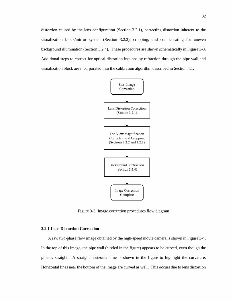
distortion caused by the lens configuration (Section 3.2.1), correcting distortion inherent to the
visualization block/mirror system (Section 3.2.2), cropping, and compensating for uneven
background illumination (Section 3.2.4). These procedures are shown schematically in Figure 3-3.
Additional steps to correct for optical distortion induced by refraction through the pipe wall and
visualization block are incorporated into the calibration algorithm described in Section 4.1.
Figure 3-3: Image correction procedures flow diagram
3.2.1 Lens Distortion Correction
A raw two-phase flow image obtained by the high-speed movie camera is shown in Figure 3-4.
In the top of this image, the pipe wall (circled in the figure) appears to be curved, even though the
pipe is straight. A straight horizontal line is shown in the figure to highlight the curvature.
Horizontal lines near the bottom of the image are curved as well. This occurs due to lens distortion
33
(Vass and Perlaki, 2003), which is a well-known phenomenon in which the magnification of the
lens is not uniform throughout the image. This type of distortion warps the image as a whole, even
though the points within the image itself are still focused (Hecht, 1998). If this distortion is
uncorrected, then shape of the interfaces detected by the algorithm will be distorted. Furthermore,
the coordinate of the pipe wall will vary in the flow direction, which will interfere with the
calibration procedure. Therefore, it is important to correct this distortion.
Figure 3-4: Raw two-phase flow image exhibiting lens distortion. Lens distortion makes the front
wall of the pipe (circled) appear to be curved. A straight horizontal line is shown to highlight the
curvature.
It is possible to remove lens distortion by simply zooming out. However, doing so will
drastically reduce the resolution of the measurement. Instead, the lens distortion is corrected using
a MATLAB function made available through the Mathworks file exchange (de Vries, 2012). Lens
distortion is a nonlinear phenomenon that can be modeled by an infinite series polynomial
(American Society of Photogrammetry, 1980). However, as long as the distortion is not severe,
34
lens distortion can be corrected using only the first term of the polynomial (Tsai, 1987), as it is
implemented in the present code. Figure 3-5 shows the effect of the lens distortion correction
procedure. Figure 3-5(a) shows an image before the lens distortion correction, and Figure 3-5(b)
shows the same image after lens distortion correction.
Figure 3-5: Lens distortion correction. (a) Image before lens distortion correction. (b) Image after
lens distortion correction.
3.2.2 Top View Magnification Correction
In the two-phase flow videos, the top view of the flow appears to be farther from the camera
than the side view. This phenomenon is illustrated in Figure 3-6, where vertical lines are
superimposed on a two-phase flow image. In the center of the image, the line touches the same
upstream edge of a small bubble, indicating that the camera is properly aligned. However, the lines
near the edges of the image do not align with features in both views. This phenomenon occurs
because the light from the top view must be reflected in the mirror, and thus must take a longer
path before reaching the camera. In Figure 3-7, this additional path length is shown schematically.
If this phenomenon is not corrected, various algorithms that compare the axial positions of the plug
bubble nose will be disrupted.
35
Figure 3-6: Raw image acquired with visualization block-mirror system, with vertical lines added
to highlight increased optical distance from camera to top view
Figure 3-7: Illustration of additional path length taken by light traveling from top view.
The top image of the flow is magnified to solve this problem. The built-in MATLAB function
“imresize” is used to magnify top view images. The image processing algorithm requires the user
to select the pixel coordinates occupied by the top view. The dimensions of the top image are then
36
multiplied by a magnification factor to obtain the corrected size of the top view image. The original
image is then projected onto the larger grid using a bicubic interpolation algorithm contained in the
“imresize” function.
The magnification factor is determined by measuring the pixel coordinates of objects in the
flow images and the physical dimensions of the visualization block. A schematic drawing of the
dimensions used is shown in Figure 3-8, and a sample image used to measure pixel coordinates is
shown in Figure 3-9. dfv is the axial length of the visualization block, and dtv is the distance between
the bolts used to hold the two halves of the visualization block together that are visible from the
top view. The subscript a denotes physical dimensions of the visualization block that are known,
and the subscript m denotes dimensions that are measured from the images.
Figure 3-8: Schematic drawing of the physical dimensions used to determine the magnification
factor.
37
Figure 3-9: Sample image used to determine magnification factor with measured dimensions
shown.
In the image, the ratio of these parameters is smaller than the ratio of the physical parameters:
𝑑𝑚,𝑡𝑣
𝑑𝑚,𝑓𝑣<
𝑑𝑎,𝑡𝑣
𝑑𝑎,𝑓𝑣
(3 − 1)
The magnification factor M can be calculated by:
𝑀 =1
𝑑𝑚,𝑡𝑣(
𝑑𝑎,𝑡𝑣𝑑𝑚,𝑓𝑣
𝑑𝑎,𝑓𝑣) (3 − 2)
The result of the top view magnification correction procedure is shown in Figure 3-10. Since
the top view magnification correction and the cropping procedure (described in Section 3.2.3) are
performed simultaneously, this image is also cropped. It can be seen from the figure that vertical
38
blue lines align with various flow features in both views, which indicates that the top view
magnification correction was performed properly.
Figure 3-10: Two-phase flow image after top view magnification correction and cropping. Vertical
lines are added to show that top view magnification correction has been performed successfully.
3.2.3 Cropping
During video acquisition, the camera is configured to make use of as much of the imaging area
as possible. However, it is not possible to configure the camera to image only the flow area, so
unnecessary portions of the image are removed in order to reduce the disk space occupied by the
saved videos and the memory used by the computer as it processed the images.
Images are cropped by simply deleting data that falls outside of the user-defined pixel
coordinates of the top view and side views of the flow. Figure 3-11 shows the result of the top-
view magnification correction and cropping procedures.
39
Figure 3-11: Image after top-view magnification correction and cropping
Although cropping is performed to remove the unused portions of the image, it is obvious from
Figure 3-11 that some portions of the pipe and visualization block are left in the image. These
features are left in the image because they are used in the calibration procedure, and because they
are helpful in providing context when viewing the flow images.
3.2.4 Background Subtraction
Although care is taken to ensure that the background illumination is as even as possible, the
background illumination is not perfectly uniform. Background subtraction is performed to
compensate for uneven background illumination. The operation compares each image of the
grayscale video of two-phase flow Tij to an image of single-phase liquid flow Fij, resulting in an
image Bij. In the present work,
𝐵𝑖𝑗𝑘 = | 𝑇𝑖𝑗𝑘 − 𝐹𝑖𝑗| , 𝑘 = 1,2 … 𝑁𝑘 (3 − 3)
Where Nk is the number of images in a video. An example of the input and output of the
background subtraction procedure is shown in Figure 3-12.
40
Figure 3-12: Input and output of background subtraction procedure
Regions of liquid-phase in the two-phase flow images have almost the same brightness as that
of the single-phase liquid background images, so these regions have near zero values in the
resulting background-subtracted image Bij. In the gas-phase, brightness values vary depending on
the orientation and surface condition of the interface between the gas and liquid phase.
The single-phase liquid background is captured using the same camera settings as the videos
of two-phase flow. Background videos 𝐹𝑖𝑗𝑘 are captured before and after two-phase flow video
acquisition in the event that the camera, lights, or diffusing sheet are inadvertently moved over the
course of the experiment. The background video is time-averaged in order to produce a single
background image.
𝐹𝑖𝑗 =1
𝑁𝑘∑ 𝐹𝑖𝑗𝑘
𝑁𝑘
𝑘=1
(3 − 4)
41
After the background video is time-averaged, it is processed using the procedures outlined in
Sections 3.2.1-3.2.3 before it is used in background subtraction.
3.3 Gas-Phase Segmentation
The ultimate goal of the current work is to measure two-phase flow parameters for plug bubbles
from two-phase flow images. This has to be done by identifying the interfaces between gas and
liquid. However, before interfaces can be found, the images must first be separated into gas-phase
and non-gas-phase (liquid-phase and background) regions. In the current work, several procedures
are performed to realize this goal in the current chapter.
3.3.1 Thresholding
In this section, the processed grayscale images as seen in Figure 3-12 are converted into a
binary (or black and white) images by comparing the local brightness values to a user-defined value
(threshold). A grayscale image can have a range of brightness values for any given pixel, whereas
a binary image can only have two brightness values for each pixel. For each grayscale image Bij, a
corresponding binary image THij is established. If the value of a pixel in the grayscale image Bij
exceeds the threshold, the corresponding pixel in THij is given a nonzero value, which means that
the pixel is occupied by the gas-phase. If it is less than the threshold, the corresponding pixel in
THij will be given a zero value, meaning the pixel not occupied by the gas-phase:
𝑇𝐻𝑖𝑗𝑘 = 0 , 𝐵𝑖𝑗𝑘 ≤ 𝐺𝑇
𝑇𝐻𝑖𝑗𝑘 = 1 , 𝐵𝑖𝑗𝑘 > 𝐺𝑇 (3 − 5)
where GT is the threshold value. A sample image produced by this procedure is shown in Figure
3-13. The threshold value GT is set by the user. As stated in the previous section, the processed
images Bij have near-zero values in the liquid-phase, but can have a range of values in the gas-phase
depending on the orientation of the interface. In the current work, GT was set to 10 (out of 255
possible brightness levels). This relatively low threshold value was applied to the background
42
subtracted images in order to detect as much of the gas-phase as possible without erroneously
detecting fluctuations in the background.
Figure 3-13: Image after thresholding
Not all of the gas-phase is detected by thresholding. Areas of the image occupied by gas-phase
will not be detected where the interface is normal to the optical axis. Consider the raw image of a
bubble shown in Figure 3-14. Near point A, the image is relatively dark. Here, the bubble interface
attenuates light because it is nearly parallel to the optical axis; light traveling through this point on
the interface will undergo total internal reflection. However, near point B, the interface is nearly
normal to the optical axis, so little attenuation occurs. As a result, point B (and points near it) have
nearly the same brightness as the single-phase liquid background. Thus, these are not recognized
as gas-phase by the thresholding algorithm, as can be seen in the thresholded image in Figure 3-14.
However, since the darker region surrounds the lighter region in the plane of the image, the object-
filling algorithm (described in Section 3.3.4) is able to recover the gas-phase regions that were not
detected by the thresholding algorithm.
43
Figure 3-14: Illustration of gas-phase regions not detected by thresholding procedure.
3.3.2 Extraneous Artifact Removal
The thresholding procedure may also incorrectly detect gas-phase regions outside the pipe area.
An example of this is shown in Figure 3-15, where regions incorrectly assigned to gas-phase are
circled. This occurs because bubbles reflect and refract light as they travel through the pipe. This
reflected light causes variations in brightness outside of the flow area, such as in the clear acrylic
pipe wall. An example of one such reflection is highlighted in Figure 3-16. In this figure, a cropped
two-phase flow image is superimposed onto a single-phase liquid background. In the right circle,
a discontinuity in the brightness can be observed at the point where the two-phase flow image meets
the background image; this difference is caused by the plug bubble. In the left circle, there is no
discontinuity in brightness because there is no plug bubble at this location in the pipe. The
reflection highlighted in Figure 3-16 can be seen in the thresholded image (Figure 3-15). While
these reflections are not likely to interfere with the measurement procedure, removing them is
simple and results in higher quality images.
The removal of these artifacts requires the user to input the pixel coordinates of the flow area.
These coordinates are also used in later procedures. After the coordinates of the flow area are
obtained, the value of any pixel outside this region is set to zero, or background. The result of this
procedure is shown in Figure 3-17.
44
Figure 3-15: Thresholded image of plug flow. Regions incorrectly assigned to gas-phase are
circled.
Figure 3-16: Image of two-phase flow superimposed on the background image. The plug bubble
is causing brightness variations in the pipe wall (right circled area). The same brightness variation
is not present downstream of the plug bubble (left circled area).
45
Figure 3-17: Image after extraneous artifact removal.
3.3.3 Curve Closing
After gas-phase regions are detected by the thresholding algorithm, bubble interfaces can be
found. Interfaces are found using the built-in MATLAB function “bwboundaries”. This function
returns interfaces as an ordered list of pixel coordinates, starting from the upper-left corner of the
image and proceeding clockwise around the interface.
This function can detect interfaces even if some of the gas-phase is incorrectly labeled as liquid-
phase. However, errors will occur if the mislabeled portion of the bubble is not surrounded by gas-
phase. An example of this is shown in Figure 3-18(b). In the figure, the detected interface is
highlighted in red. Errors in the detection of this interface have two causes. The first, which is
highlighted by arrow 1, occurs because the edge of the bubble is not detected by the thresholding.
The reason for the failure of the thresholding algorithm can be observed in Figure 3-18(a); the
interface is nearly the same brightness as the background near the defect. This type of defect is
corrected through procedures described in Sections 3.3.3.1 and 3.3.3.3. The second cause, which
46
is highlighted by arrow 2, occurs because the bubble is partially outside the field of view. This is
corrected by the procedure described in Section 3.3.3.2.
Figure 3-18: Effect of curve closing on boundary detection. (a) Flow image. (b) Thresholded
image with detected boundaries highlighted in red.
3.3.3.1 Morphological Closing
The present chapter discusses morphological closing, which is used to fix defects resulting
from the thresholding procedure. These defects are discussed in the preceding section and
highlighted by arrow 1 in Figure 3-18(b). Morphological closing belongs to a class of well-
established image processing algorithm known as a morphological transformations. The
information in the present chapter is only intended to briefly summarize the mechanism of
morphological closing with respect to binary images, but more detailed information regarding
morphological transformations can be found in Sonka et al. (2015).
All morphological transformations follow the same general procedure. They operate by
comparing a small set of points known as a “structuring element” to the image. These comparisons
are made for every pixel by superimposing the structuring element on each pixel. Different
morphological transformations make different comparisons and alter the image in different ways.
One of the points in the structuring element is designated as the “origin”. In this context,
“origin” does not necessarily refer to the center of the structuring element, but rather a point in the
structuring element that is given special significance. The significance differs depending on the
47
morphological operation being considered. Before proceeding with the description of
morphological closing, it should also be noted that the terms “foreground” and “background” are
used to refer to the two regions of the binary image, rather than “gas-phase” and “non-gas-phase”,
as in the rest of the current work.
Morphological closing is achieved by performing two simpler morphological transformations
in series. The first morphological transformation is called dilation, and the second morphological
transformation is called erosion. Before closing is discussed further, dilation and erosion will be
discussed individually.
Dilation expands the foreground regions of the image. A schematic of the dilation procedure
is shown in Figure 3-19. Like all morphological transformations, dilation is performed by
systematically superimposing the structuring element to each pixel in the image. When the origin
of the structuring element coincides with a background pixel, no change is made to the resulting
image (Case I). Otherwise, each pixel inside the structuring element in the resulting image is
converted to foreground. (Case II). In the final result shown in Figure 3-19, pixels added to the
foreground region by dilation are shaded. Pixels that effected changes in the final image are
highlighted by red “x”s.
Erosion shrinks the foreground regions of the image. This process is shown schematically in
Figure 3-20. In erosion, the pixel at the origin of the structuring element in the resulting image will
remain a foreground pixel as long as every pixel inside the structuring element in the original image
is also foreground. (Case I). Otherwise, the pixel at the origin is converted to background. (Case
II). In the final result, the pixels converted to background by erosion are shaded. Pixels that
effected changes in the final image are highlighted by red “x”s.
48
Figure 3-19: Illustration of dilation transformation.
49
Figure 3-20: Illustration of erosion transformation.
The closing transformation is a dilation transformation followed by an erosion transformation
with the same structuring element. As stated earlier, it can be used to fill small gaps between
50
foreground regions. An example of this procedure is shown in Figure 3-21. In the figure, the
original image (a) is first dilated by the structuring element shown in (b). The result is shown in
Figure 3-21(c), where the original image is outlined in orange and the pixels added by dilation are
shaded. Pixels that effected changes in the final image are highlighted by red “x”s. Next, erosion
is applied to the (c), and the result is shown in (d). In (d), the original image is again outlined in
orange, and the foreground pixels removed by erosion are shaded, and pixels that altered the
resulting image are highlighted with red “x”s. The final result without highlights is shown in (e).
In the example, the two foreground regions in the bottom of the image are connected by the closing
procedure. However, the small foreground pixel in the upper-right corner is not connected by the
closing procedure because it is too far from the other foreground regions. Apart from this, the
original image is unchanged by the closing procedure.
Figure 3-21: Illustration of morphological closing procedure
51
The size and shape of the structuring element changes the behavior of the morphological
transformations. The size of gaps filled by closing is directly related to the size of the structuring
element used in the transformation; using a larger structuring element will fill larger gaps.
However, using a larger structuring element also means that dispersed bubbles are more likely to
be erroneously “connected” to the plug bubble interface by this algorithm. In the present work, the
size of the structuring element used in morphological closing nMC is set to the smallest possible
value that yields a symmetric element (a 3x3 square with the origin in the center). Physically, this
corresponds to an element with a side length of 0.9 mm. It is found that this element is sufficient
to fill most gaps present after thresholding. This treatment ensures that the boundary complete
procedure (described in Section 3.3.3.3), which fills larger gaps, can operate correctly.
3.3.3.2 Inlet and Outlet Line Drawing
As stated in Section 3.2.4, regions near the edge of the bubble are dark because the interface is
nearly parallel to the optical axis, which causes a great deal of light to undergo total internal
reflection (see Figure 3-14). However, when a portion of the bubble is outside of the viewing area,
this dark edge will not be imaged. Almost all of the plug bubbles in the present experiment are
longer than the viewing area, so this phenomenon affects almost all of the measured plug bubbles.
To compensate for this, the most downstream and the most upstream pixels within the pipe in
the binary image are converted to foreground, effectively drawing lines at the inlet and outlet of
the viewing area. In this way, any bubble that is partially outside the viewing area will still be
recognized as a closed curve.
3.3.3.3 Boundary Completion
Boundary completion is the final step in the set of curve closing procedures. It is similar to
morphological closing (see Section 3.3.3.1) in that it corrects the defects in the image caused by
fluctuations in the brightness of the interface. However, this procedure is intended to correct larger
gaps than morphological closing.
52
This algorithm uses the built-in MATLAB function “bwboundaries” (see Section 3.3.3) to find
the boundaries of gas-phase regions. To detect these gaps, the algorithm collects the points with
the lowest y-coordinate for every given x-coordinate on the detected interface. Then, the code
examines the path length of interface between each minimum y-coordinate and the minimum y-
coordinate at the adjacent x-coordinate. This process is illustrated in Figure 3-22. In this figure,
red, white, and blue pixels represent the gas-phase. The boundary detected by “bwboundaries” is
highlighted in red, and the points on this boundary with the minimum y-coordinates are highlighted
in light blue. The image on the left shows a bubble that does not need correction, and the image
on the right shows a bubble with a defect (A) that would interfere with the detection of the interface.
In the right image, paths analyzed by the “boundary completion” algorithm are also shown.
Paths 1, 2, and 4 are the same in both images. However, path 3 (at the location of the defect) is
significantly longer because the artificial “hole” boundary must also be traversed. The code
identifies defects in the boundary when this path length exceeds a user-supplied threshold pBC.
Because the path length near a defect will be significantly longer than normal path lengths, the
output of this algorithm is fairly insensitive to the selection of this threshold. In the present work,
any path length longer than 10% of the interface’s perimeter was identified as a defect. Once a
defect has been identified, the code draws a line between the point before the defect and the nearest
minimum y-coordinate, closing the defect. The procedure is then repeated with the maximum y-
coordinates considered instead of the minimum y-coordinates.
53
Figure 3-22: Illustration of "boundary complete" algorithm
This procedure may falsely identify gaps in the boundary if the plug bubble is in contact with
a small dispersed bubble, as this may induce a sudden change in the minimum y-coordinate of the
interface. An example of such a case is shown in Figure 3-23. Following through with the
boundary complete procedure when such a gap is detected would result in unphysical changes to
54
the bubble interface. For this reason, before a defect is closed with the boundary complete
algorithm, the shape of the portion of the interface that will be removed is compared with the shape
of the plug bubble interface and the shape of the “hole” boundary in the previous frame. If the
portion of the interface to be removed is more similar to the “hole” boundary, then the procedure
is performed. Otherwise, the procedure is not performed.
Figure 3-23: Example of a case where a bubble in contact with the plug bubble induces a sudden
change in the minimum y-coordinate. The detected interface is highlighted in red, and the minimum
y-coordinates are highlighted in blue.
Procedures performed in the curve closing section allow the bubble interfaces to be detected
accurately despite deficiencies in the thresholding. An example of the improvement made by these
techniques is shown in Figure 3-24.
Figure 3-24: Example of improvement in interface detection from curvature closing techniques.
(a) Interface detected before curve closing. (b) Interface detected after curve closing.
55
3.3.4 Object Filling
The steps outlined in Section 3.3.3 are performed to ensure that the gas-phase regions detected
through the thresholding procedure completely enclose the gas-phase regions that are not detected
by thresholding. The procedures in this section are used to correct the erroneously detected pixels
so that in the resulting black and white image, one group of pixels corresponds to the gas-phase
and the other corresponds to the liquid-phase.
This function first uses the built-in MATLAB function “bwboundaries” to obtain the gas-liquid
interface projected into the plane of the image. Then, the function determines which pixels are on
the interior of the interface by counting the number of times the interface crosses a line between
each pixel and a pixel known to be on the exterior of the object. If there are zero or an even number
of crossings between the exterior and the given pixel, then the pixel is on the exterior. Otherwise,
the pixel is inside the interface and is designated as gas-phase.
3.4 Identification and Tracking of Plug Bubbles
In Section 3.3, corrected images were converted into binary images in which gas-phase regions
are segmented from liquid-phase and background regions. From each of these images, interfaces
are obtained using the built-in MATLAB function “bwboundaries”, as explained in Section 3.3.3.3.
In order to measure plug bubble parameters, plug bubble interfaces must be distinguished from
other gas-liquid interfaces, interfaces belonging to the same plug bubble at different points in time
must be associated with each other, and similarly, interfaces seen from the top and side views must
be associated with each other.
To distinguish plug bubble interfaces from other gas-liquid interfaces, a simple bubble length
criterion is used. The image processing code measures the bubble length as the axial distance
between the most downstream point and the most upstream point on the bubble. Interfaces longer
than two pipe diameters in the flow direction are classified as plug bubbles, all shorter interfaces
are discarded. The value of this threshold was developed empirically by manually measuring the
56
lengths of 50 plug bubbles using flow visualizations and velocity measurements from the local
four-sensor conductivity probe for one flow condition. While this threshold has been sufficient for
the development of the image processing algorithm, a threshold based on the physics of plug flow
is desirable and should be obtained in the future.
A tracking algorithm is used to associate interfaces belonging to the same plug bubble that are
detected at different points in time. For each plug bubble interface detected at the inlet of the
viewing area, the tracking algorithm finds corresponding interfaces in subsequent video frames.
The algorithm works recursively; the plug bubble interface detected in the nth frame will be used to
find the plug bubble interface in the nth+1 frame until the plug bubble exits the viewing area.
Since the tracking algorithm is recursive, failing to identify a plug bubble interface in one frame
will cause the tracking algorithm to fail and the bubble to be discarded. Therefore, this algorithm
must be robust. Three methods are employed to identify appropriate plug bubble interfaces in
subsequent frames. The first method is based on tracking the plug bubble nose. The nose of the
plug bubble is defined as the most downstream point on the plug bubble. In the images, the most
downstream pixels in the detected plug bubble interface constitute the nose. Finding the position
of the plug bubble nose in the flow direction is trivial. However, if multiple pixels occupy the most
downstream position, the nose position in the lateral direction is ambiguous. In this case, the
positions all pixels in the plug bubble nose are averaged to obtain a lateral nose position.
To track the plug bubble interface, the code identifies the nth+1 frame interface as that which
encompasses the nth frame bubble nose. Due to the high frame rates used in capturing two-phase
flow visualizations, plug bubbles will only advance a small fraction of their length between the nth
frame and the nth+1 frame, allowing the first method to identify the nth+1 frame interface correctly
in the majority of cases. However, this method may fail if the plug bubble nose moves
perpendicular to the flow direction, in which case the coordinate of the plug bubble nose in the nth
frame may not be encompassed by the interface in the nth+1 frame.
57
If the first method fails, a second method is employed to identify the nth+1 frame interface as
that which encompasses the center of the plug bubble in the nth frame. The center of the plug bubble
is calculated as the mean of the coordinates of the bubble interface. Like the first method, this
method is based on the principle that the plug bubble will not advance more than its length between
successive frames.
If the first and second methods both fail, a third tracking method is employed. This method
finds the interface in the nth+1 frame with the most similar shape and position to that in the nth
frame. This method is similar in principle to the chamfer matching technique developed by Barrow
et al. (1977) for finding similar shapes in different images. A measure of similarity between the
two interfaces is calculated by averaging the smallest distances between the discrete points that
make up the two bubble interfaces. Smaller values of the resulting parameter correspond to more
similarly shaped and positioned interfaces. Because it incorporates information from all points on
each interface, this method is relatively reliable, although it is time-consuming. After calculating
the shape similarity parameter for all interfaces in the nth+1 frame, this method returns the interface
that is most similar to the plug bubble interface in the nth frame.
Because small bubbles may exist near the plug bubble interfaces, it is possible for the tracking
algorithm to erroneously associate the interface of a small dispersed bubble in the nth+1 frame with
the plug bubble interface in the nth frame. To prevent this from occurring, an additional algorithm
rejects interfaces in the nth+1 frame that have a perimeter less than a percentage preject of the plug
bubble perimeter in the nth frame. Here, the perimeter is essentially used as a measure of bubble
size. The perimeter is used instead of other measures because it can be calculated quickly. The
minimum perimeter preject is set to 50% in the present work. If the interface of a small bubble is
selected, it is expected that the perimeter will be much smaller than 50%, so the outcome of this
algorithm should be relatively insensitive to this parameter. In rare cases, the perimeter of the plug
bubble interface may actually decrease by 50% between frames. For example, this may occur if
58
two plug bubbles are initially in contact and then separate. To accommodate this occurrence, the
tracking algorithm will allow the perimeter to decrease by half if the same interface is detected by
both the third method, which is thought to be the most robust, and either the first or the second
method.
A flow chart showing the logic used in the tracking algorithm is shown in Figure 3-25, and a
sample result of the tracking algorithm is shown in Figure 3-26. The figure shows a two-phase
flow image of a plug bubble. The interfaces obtained by the tracking algorithms are outlined in
blue and green. Interfaces detected earlier are shown in blue and those detected later are outlined
in green. Since the nose position of the plug bubble is also detected by the tracking algorithm, the
nose of each interface is circled in red, and red lines are drawn between the successive nose
positions.
59
Figure 3-25: Flow chart showing tracking algorithm logic.
Figure 3-26: Series of interfaces and nose positions obtained by the tracking algorithm.
60
After the tracking procedure, an additional algorithm is employed to associate plug bubble
interfaces detected in the side view with those detected from the top view. This is referred to as
the pairing algorithm. Any sets of plug bubble interfaces sharing axial nose positions within a user-
defined threshold at the same point in time are associated with each other. In rare instances, plug
bubbles will collide in the viewing area, leading to ambiguity in this algorithm. Since this
occurrence is rare, these interfaces are discarded by the code. Pairing may also fail if the tracking
algorithm fails in either the side or top view, in which case the bubble in the remaining view will
be discarded. The threshold for the pairing algorithm was determined by initially setting the value
to 0, and then increasing the threshold until all bubbles (except the cases listed above) were paired.
This value is set to 4 pixels, or 1.2 mm in the present work. It is expected that increasing the value
further would have little to no effect on the pairing algorithm
3.5 Contacting Bubble Segmentation
The procedures described in the preceding sections yield coordinates of plug bubble interfaces
from raw two-phase flow videos. However, the preceding algorithms are not able to distinguish
plug bubble interfaces from interfaces of small bubbles that contact the plug bubble. An example
of such a contacting bubble is shown in Figure 3-27. These sections contain algorithms designed
to make this segmentation. The procedure described in Section 3.5.1 is designed to segment plug
bubbles that collide with the plug bubble within the viewing window. Conversely, the algorithms
in Section 3.5.2 are designed to segment small bubbles that are already in contact with the plug
bubble when they enter the viewing window. Section 3.5.3 describes algorithms designed to
segment bubbles too small to be segmented by either earlier method.
All of the procedures outlined in this section involve finding breakpoints, or the two points on
the detected interface where the individual bubbles are in contact. Once breakpoints are found, a
61
procedure is invoked to connect the breakpoints in order to recover the true interface of the plug
bubble.
Figure 3-27: Example of a small bubble contacting the plug bubble
3.5.1 Distance Check
As a plug bubble travels down the pipe, it will overtake the slower dispersed bubbles in front
of it. When such a collision occurs in the viewing window, the interface detected by the image
processing software will instantaneously jump forward. A particularly obvious example of this
phenomenon is pictured in Figure 3-28, where a plug bubble overtakes a cluster of small, dispersed
bubbles in the nth frame. Because the two-phase flow images are captured at a high frame rate,
these sudden position changes can be used to detect and segment small bubbles because they
correspond to unrealistically large velocities.
The algorithm operates by calculating the smallest distance to the previous interface n-1 for
each discrete point in the present interface n. Before the distance is calculated, interface n-1 is
displaced forward according to the mean propagation velocity of the plug bubble nose under
consideration. In this way, only the fluctuating component of velocity is considered. Calculated
62
distance values are then compared to a threshold; portions of the detected interface exceeding the
threshold are considered to have resulted from a collision with a small dispersed bubble and are
flagged for removal.
Removing the portion of the detected interface belonging to a small dispersed bubble requires
finding the points on the detected interface where the dispersed bubble and the plug bubble are in
contact, or the breakpoints. For each portion of the interface that is flagged for removal,
breakpoints are found by stepping away from the dispersed bubble along the detected interface until
a point is found that is shared with the displaced interface n-1. The portion of the current interface
between the two breakpoints is then removed and replaced with that of the n-1 interface between
the breakpoints. In the event that no point on the n interface is shared with the n-1 interface, the
breakpoints will be connected with a straight line.
Figure 3-28: Change in detected interface as plug bubble overtakes dispersed bubble cluster
(detected interface highlighted in blue).
Because the local velocity of the interface fluctuates, the distance from the displaced previous
boundary to the current boundary may be nonzero even if no collision occurs. For this reason,
distances smaller than a threshold value ddist are ignored. In the present work, distances greater
63
than 6 pixels, or approximately 1.8 mm are flagged for removal. It was found that setting the
threshold to a smaller value would cause actual fluctuations in the interface to be removed. Because
of this threshold value, this algorithm will not be able to detect collisions with bubbles less than
1.8 mm in diameter. In view of this, the convex curvature segmentation algorithm is developed to
complement the distance check algorithm. This algorithm is applied after the off-screen collision
procedures and described in Section 3.5.3.
3.5.2 Off-screen Collision Procedures
This set of procedures, referred to as “Off-screen Collision” procedures, are designed to
segment bubbles when the plug bubble enters the viewing area with a small bubble entrained and
in contact. An example of this case is shown in Figure 3-29, where a small dispersed bubble (circled
in red) is entrained by the plug bubble when it enters the frame, and is carried across the viewing
window. To recover the plug bubble interface in these cases, two methods to detect breakpoints
are implemented in parallel, and then the validity of the breakpoints is checked by comparing the
methods with each other. After application of these breakpoints, criteria are implemented to
enforce agreement between the nose positions observed in the top view and the side view, and to
attempt to extrapolate the breakpoints detected to later frames. The algorithm outlined in Section
3.5.2.1 detects breakpoints by identifying the interface shared by bubbles in contact, and the
algorithm in Section 3.5.2.2 detects breakpoints using the curvature of the detected interface.
64
Figure 3-29: Dispersed bubble entrained by plug bubble without coalescing
3.5.2.1 Adaptive Threshold / Image Skeleton Breakpoint Detection
The algorithm described in the present section finds breakpoints by detecting the interface
shared by the plug bubble and dispersed bubbles that are in contact. Like all air-water interfaces,
this interface manifests itself as a dark region in the grayscale image; the present algorithm detects
this dark region through the application of an adaptive threshold to the image brightness. This
procedure is similar in principle to the thresholding procedure used to detect gas-phase regions
described in Section 3.3.1. However, the present procedure needs to detect the light region in the
center of the bubble reliably, (see Figure 3-14) in order to identify the contacting interface. Because
of this additional requirement, the global threshold used in the gas-phase detection algorithm is
replaced with an adaptive threshold.
Adaptive threshold algorithms define a unique threshold value for each pixel based on the
characteristics of the surrounding region. In the present work, the adaptive threshold is set as the
65
mean brightness value of the n x n group of pixels surrounding the pixel under consideration. An
illustration is shown in Figure 3-30. In the figure, the threshold for the pixel marked with the red
x is calculated using the pixels highlighted in green. The same size neighborhood is used for all
pixels in the image, apart from those near the edge of the image, where a reduced size neighborhood
must be used. The image resulting from the adaptive threshold is shown in the figure on the right.
This algorithm allows both dark and light regions of the bubble to be detected as long as there
is contrast between the center of the bubble and the edge of the bubble, and the adaptive threshold
neighborhood includes both dark and light regions. The adaptive threshold algorithm also
inherently compensates for varying levels of brightness of the interface across the image, since
every point is referenced to points in the surrounding region.
In regions of relatively uniform brightness, the locally defined threshold is not meaningful, so
the algorithm produces noisy output. This noisy output is removed by computing the intersection
between adaptive threshold images and filled images (described in Section 3.3.4). This is shown
in Figure 3-29. A comparison of an image produced by the global threshold and an image produced
by the adaptive threshold procedure is also shown in the figure.
Figure 3-30: Illustration of adaptive threshold principle
66
Figure 3-31: Comparison of global and adaptive threshold
In the present work, the size of the neighborhood nAT used in the adaptive threshold algorithm
is set to 21 pixels. The resulting 21x21 square element corresponds to a 6.3x6.3mm square region
in the image. As was mentioned earlier, the adaptive threshold will yield an acceptable result as
long as the neighborhood incorporates both light and dark regions of the bubbles, so a wide range
of neighborhood sizes should yield an acceptable result. In Figure 3-32, an image is processed with
several different neighborhood sizes to show the effect on the resulting image.
67
Figure 3-32: Comparison of results of adaptive threshold algorithm with different neighborhood
sizes
After the adaptive threshold is employed, the morphological closing algorithm described in
Section 3.3.3.1 is applied to the images in order to close small gaps. Then, an algorithm is
employed to reduce the thickness of the interfaces found by the adaptive threshold algorithm to 1-
2 pixels, leaving what is known as an image skeleton. This portion of the code uses a modified
version of the “MB2” thinning algorithm developed by Bernard and Manzanera (1999). This
algorithm iteratively removes pixels from an image without changing the topology of the black and
white image. In other words, the algorithm will not merge any background regions as it thins the
foreground. The MB2 algorithm was also developed so that the resulting image skeleton will lie
in the center of the original shape. However, in its present implementation, the outer interface of
the plug bubble is preserved in the image skeleton so that breakpoints can be detected and compared
to those detected with the concave curvature algorithm. All other portions of the image skeleton
will lie at the center of the interface detected by the adaptive threshold algorithm. Figure 3-33
shows the result of the MB2 thinning algorithm with the original image superimposed.
68
Figure 3-33: Result of modified "MB2" thinning algorithm with original image superimposed
Once the interface is reduced to a 1-2 pixel thickness, breakpoints are identified by finding
portions of the image skeleton that touch the outer boundary in at least two locations. From Figure
3-33, it can be observed that small holes in the interface detected by the adaptive threshold
algorithm create small “loops” in the image skeleton, which can in turn result in the detection of
erroneous breakpoints. To help alleviate this problem, two separate closing element sizes are
applied to the adaptively thresholded images, and breakpoints from these are detected in parallel.
Only breakpoints that appear in both images are retained. Examples of erroneous breakpoints
eliminated by this step are shown in Figure 3-34.
Figure 3-34: Illustration of benefit of using parallel closing element sizes. Some erroneous
breakpoints will only be detected in the 3x3 closed image (circled in red), and other will only be
detected in the 5x5 closing element image (circled in blue).
69
As stated above, for a bubble to be segmented by the adaptive threshold algorithm, both the
dark edge of the bubble and the light center of the bubble must be detected. Since the closing
algorithm removes small background regions from the image, it can prevent small bubbles from
being detected. To maximize the amount of bubbles that can be detected, the two smallest
symmetric closing element sizes were used in the present work. The sizes of these elements nMC
and nMC2 are 3 and 5 pixels, which correspond to 0.9x0.9 mm and 1.5x1.5 mm square elements,
respectively.
It is desirable to estimate the smallest bubble size that can be detected for a given closing
element size. Consider an air bubble in water under uniform, parallel lighting conditions. In the
center of the bubble, light will pass through with little attenuation. However, where the angle of
incidence for light passing through the air-water interface exceeds the critical angle, light will be
undergo total internal reflection, creating a dark region in the image. For air and water, the critical
angle can be calculated using the respective indices of refraction:
𝜃𝑐 = arcsin (𝑛𝑎𝑖𝑟
𝑛𝑤𝑎𝑡𝑒𝑟) = arcsin (
1
1.3) = 50.3° (3 − 6)
A scaled depiction of this for a spherical air bubbles in water is shown in Figure 3-35.
Assuming a spherical geometry, the diameter of the transparent area of the bubble dtrans can be
related to the physical diameter of the bubble d:
𝑑𝑡𝑟𝑎𝑛𝑠 = 0.77𝑑 (3 − 7)
Drawings of bubbles with this modeled geometry are displayed alongside actual bubble images
in Figure 3-36. Based on the closing element sizes used in the present algorithm, the smallest
bubble that can be correctly segmented by the adaptive threshold algorithm is 2.8 mm.
70
Figure 3-35: Scaled depiction of total internal refraction for a spherical air bubble in water
Figure 3-36: Bubble images compared to images generated assuming spherical bubbles and parallel
lighting
Since the adaptive threshold / image skeleton detection method detects the contacting interface
between plug bubbles and small dispersed bubbles, it naturally produces breakpoint pairs.
However, this method may also falsely detect breakpoints when the adaptive threshold does not
operate perfectly. It is desirable to verify the results of this method with an additional method; the
concave curvature breakpoint detection method was developed for this purpose.
71
3.5.2.2 Concave Curvature Breakpoint Detection
The concave curvature breakpoint detection algorithm uses the curvature of the detected bubble
interface to identify dispersed bubbles in contact with the plug bubble. In general, the curvature 𝜅
for any curve in a 2-D plane can be expressed as
𝜅 =𝑑𝜃
𝑑𝑠(3 − 8)
Where θ(s) is the angle tangent to the curve and s is the parameterized distance along the curve.
Since the curves analyzed in the present work are discrete, the calculation of the curvature must
also be discretized. In the present work, a central differencing scheme is employed to calculate the
discrete derivatives. However, since the angle between two adjacent points in a discrete image may
only vary in increments of 45°, a smoothing factor k must be employed to calculate the angle at a
given point accurately. The method described by Freeman and Davis (1977) is employed to
approximate the angle tangent to the interface. For a given point i with an arbitrary smoothing
factor k, the line tangent to the curve is approximated by drawing a line between points i-k and i+k,
and the angle θ is calculated as the angle of this line. The discrete curvature at point i is then
calculated as
𝜅𝑖 =(𝜃𝑖+1 − 𝜃𝑖−1)
𝛿𝑠𝑖
(3 − 9)
Where δsi is the path length between points i+1 and i-1. In general, the sign of the curvature
will differ depending on whether the angle tangent to the curve θ changes in the clockwise or
counter-clockwise direction. For a closed curve, the sign of the local curvature with a given
parameterization also indicates whether the curve is locally concave or convex. Based on the
parameterization and sign conventions adopted in the present work, positive curvature corresponds
to convex curves, and negative curvature corresponds to concave curves.
72
Figure 3-37(a) shows curvature values calculated for the interface depicted in Figure 3-37(b).
When two bubbles overlap, their outline may have a sharp, concave curvature that is not typically
observed in individual bubbles, as is illustrated in Figure 3-37(b). These sharp concave shapes are
reflected as a large negative curvature values; thus, the curvature can be used to detect breakpoints.
In Figure 3-37(a) and (b), points with large negative curvature values exceeding a threshold are
highlighted with red circles.
In the present work, the smoothing parameter for the concave curvature calculation kconc and
the magnitude of the concave curvature threshold Tconc were set by qualitatively evaluating the
results obtained from various parameter values. In the future, more work should be performed to
justify these parameter settings.
Breakpoints detected by the curvature method are compared with those detected by the adaptive
threshold method to segment bubbles.
Figure 3-37: (a) Curvature calculated along detected interface shown in (b). Pixel indices begin in
the lower right corner and increase in the clockwise direction. Local minima exceeding a threshold
are highlighted. (b) Detected interface featuring overlapping bubbles.
3.5.2.3 Breakpoint Verification and Interpolation
Both the methods of breakpoint detection may falsely detect breakpoints. In order to avoid
incorrectly segmenting bubbles based on false positives, breakpoint pairs given by the adaptive
threshold / image skeleton method are verified with those found by the concave curvature method
before segmentation is carried out. For every adaptive threshold / image skeleton breakpoint, the
73
code searches for a concave curvature breakpoint within a user-defined radius. If such a breakpoint
can be found, then the point is considered to be verified. If not, the point is unverified.
Based on this verification step, breakpoint pairs are classified into one of three categories. If
both breakpoints in an adaptive threshold / image skeleton pair can be verified, the pair is classified
as a “verified pair.” If only one breakpoint can be verified, the pair is classified as a “half-verified
pair”, and if neither point can be verified, then the pair is classified as an “unverified pair”.
Verified pairs of breakpoints can be used to segment contacting bubbles with high confidence.
However, due to imperfections in the breakpoint detection algorithms, verified breakpoints
typically cannot be found in every frame where a small bubble contacts the plug bubble. To
compensate for this, the code attempts to associate half-verified breakpoints detected at different
points in time with verified breakpoints. For each verified pair, the code will search in subsequent
and previous images until a half-verified or verified pair of breakpoints can be found within the
vicinity. In searching for nearby breakpoints at different points in time, the code translates the
breakpoints according to the mean velocity of the plug bubble nose under consideration. Whenever
a matching pair of verified or half-verified breakpoints is found, that pair (instead of the original
verified pair) will be used in subsequent searches until an additional pair is found. This allows the
code to detect contacting bubbles that move relative to the plug bubble.
In this way, verified or half-verified breakpoint pairs detected at different instances in time are
associated with each other. However, often verified or half-verified pairs can be associated with
each other at some instance tn and then at a later instance tn+k, but no breakpoint pairs can be found
in times tn+1 through tn+(k-1). In these cases, breakpoints are linearly interpolated between frames tn
through tn+k so that contacting bubbles can be segmented in the intervening period. The result is an
uninterrupted set of breakpoint pairs from the first detected pair at time tF to the last detected pair
found at time tL. This procedure is repeated until all verified breakpoint pairs have been considered
or associated with each other.
74
Similarly, there will typically be a period between the time tL when the last pair of verified or
half-verified breakpoints is detected and the time te when the contacting interface exits the field of
view. It is ambiguous whether this corresponds to a failure of the breakpoint detection algorithms
or a coalescence between the plug bubble and the contacting bubble. To resolve this ambiguity,
several additional steps are performed to find breakpoints after time tL, which are described in
Section 3.5.2.4.
3.5.2.4 Breakpoint Extrapolation and Side/Top View Consistency Check
At this stage in the processing algorithm, breakpoints can be applied to the images,
segmenting the small bubble interface from the plug bubble interface. Breakpoints are applied
sequentially, starting from the first image when the plug bubble enters the viewing window and
proceeding to later images. However, before proceeding, algorithms described in the current
section are applied to check the validity of the segmentation.
The first check performed is the breakpoint extrapolation algorithm. This algorithm is similar
in principle to the algorithm used to associate verified and unverified pairs detected at different
points in time. After the last frame of a set of verified/half-verified breakpoints, this algorithm
searches in subsequent frames for any breakpoints (verified or unverified) near a predicted
breakpoint location. As before, the breakpoint location is predicted by translating the previous
breakpoints according to the mean velocity of the plug bubble. However, the algorithm will only
search for breakpoints in a limited number of subsequent frames; the number of frames tBP is an
input parameter. In the current work, this parameter is set to 10 frames or 0.005 seconds. This
value was selected by qualitatively evaluating the results obtained from various parameters.
Since the nose of the plug bubble is always visible from the top and side view, the detected
axial position of the plug bubble nose should always agree unless the segmentation was not carried
out correctly. So, the code will also check to ensure that the axial positions of the plug bubble nose
from the top and side view agree with each other within a certain margin. Should the nose
75
positions disagree, the code will apply any breakpoints (verified or unverified) on the more
downstream interface that are near the axial position of the upstream nose and make the nose
positions agree. The margin by which bubble noses are permitted to disagree dnose is set by the
user. In the present work, this value is set to that of the distance check threshold, i.e. 6 pixels, or
1.8 mm.
As stated above, a breakpoint pair may disappear if a coalescence occurs between a contacting
bubble and the plug bubble, or if the breakpoint detection algorithm fails. However, if a breakpoint
pair disappears due to bubble coalescence, it should disappear simultaneously in the top view and
the side view. Thus, if a breakpoint pair is detected at time tn in the side and the top view but
disappears at time tn+1 in only one view, then it can be said that a bubble coalescence has not
occurred, but the segmentation algorithm has failed. In this case, the breakpoints from time tn are
translated according to the mean velocity of the plug bubble under consideration and applied in
frame tn+1.
Several steps in the current algorithm require the code to evaluate whether breakpoints
correspond to each other based on their proximity. For simplicity, the same distance threshold rBP
is used to make all of these evaluations. The position of breakpoints will naturally fluctuate in
time; in addition, the position of some breakpoints will be altered by the closing algorithm used in
the adaptive threshold / image skeleton breakpoint detection technique. Accounting for both of
these uncertainties, a radius of 10 pixels, or 3mm is used in searching for equivalent breakpoints.
3.5.3 Convex Curvature Segmentation Algorithm
The convex curvature segmentation algorithm uses the curvature of the detected bubble
interface to detect collisions with dispersed bubbles. The curvature was defined in Section 3.5.2.2,
where it was used in a method to detect breakpoints. The current method seeks to detect relatively
small dispersed bubbles. The curvature is directly related to the radius of curvature R, or the radius
of a circle that best approximates the curve at that point:
76
𝜅 =1
𝑅(3 − 10)
Therefore, the interface of small bubbles will exhibit a large curvature value. As described in
Section 3.5.2.2, that value will also be positive in the present work because the curvature is convex.
To segment small bubbles from the image of the plug bubble, the curvature is calculated at each
point along the detected interface. Then, portions of the interface where the curvature exceeds the
threshold are flagged for removal. Breakpoints are identified as the local curvature minima
surrounding the points exceeding the curvature threshold. The removed interface is then replaced
with a straight line connecting the two breakpoints. Because replacing portions of the interface
with straight lines method can create unphysical corners in the detected interface, this procedure is
performed iteratively until no portions of the interface exceed the curvature threshold.
Because of the inversely proportional relationship between the curvature and the radius of the
small bubble, this method should be more effective at segmenting small bubbles. As such, this
method is a natural complement to the method described in Section 3.5.1, which is more effective
at segmenting large bubbles. The convex curvature threshold Tconv is set to 1.11 rad/mm, which
should allow detection of bubbles with a diameter less than 1.8 mm, complementing the algorithm
described in Section 3.5.1.
A limit in the effectiveness of the current method is reached when the bubble becomes too
small to calculate the curvature around the projected interface accurately. This is related to the
smoothing parameter kconv (see Section 3.5.2.2), which dictates how many points are used in the
curvature measurement. To minimize the number of points required in the curvature calculation,
the smoothing parameter is kept at the minimum value (1) for the convex curvature algorithm. At
this value, bubbles less than 0.5 mm in diameter may escape detection by the convex curvature
method.
77
In Figure 3-38 an example of an interface detected by this procedure is superimposed (in red)
on the two-phase flow images.
Figure 3-38: Example interface produced by contacting bubble segmentation. Interface is
highlighted in red.
78
Chapter 4
Measurement of Two-Phase Parameters and Benchmarking
While the image analysis code is able to measure detailed coordinates of plug bubble interfaces,
this information is not useful unless the code can use this information to measure two-phase flow
parameters. The current chapter explains the algorithms implemented to measure two-phase flow
parameters from detected interfaces of plug bubbles.
4.1 Calibration
Before two-phase parameters of plug bubbles can be measured, calibration of the spatial
coordinates must be performed. This step is necessary because plug bubble interfaces are stored in
pixel coordinates; for measurements to be performed, these pixel coordinates must be related to a
physical coordinate system. Calibration is performed in both the flow direction (axial direction)
and the lateral direction (perpendicular to the flow direction or in the image plane). In the axial
direction, a single calibration factor applies of the entire viewing area. Calibration in the lateral
direction is more complicated because of the optical distortion induced by the curved acrylic pipe
wall. To compensate for this, look-up tables and a simple ray-tracing program are implemented in
the lateral calibration.
In both the axial and lateral calibration procedures, the effect of refraction must be accounted
for. In this work, the “Pinhole Camera” model is used to relate the apparent positions (or positions
within the image) of objects to their true positions in the pipe. This is shown in Figure 4-1 . Here,
the camera is modeled as a small hole, such that the apparent position (x1 and x2 in the figure) can
be found by tracing a ray from the object, through the small hole to the image plane (Jähne, 1997).
In this model, the apparent position can be related to the angle of the ray traveling from the object
through the camera. This allows the true positions of objects to be related to their apparent positions
through ray tracing, which accounts for the effects of refraction. A simple example of ray tracing
79
is shown in Figure 4-2, where refraction through the flat interface causes the true and apparent
positions of the object to differ. However, since the position of the material interface, the object,
and the camera are all known, the refraction can be accounted for analytically.
Figure 4-1: Schematic description of pinhole camera (from Jähne, 1997). Apparent positions of
objects are related to the angle of the ray entering the camera.
Figure 4-2: Differing true and apparent position caused by refraction
80
4.1.1.1 Axial Calibration
In the axial direction, a single calibration factor can be used throughout the entirety of the
viewing area. This can be justified by analytically considering the optical distortion in the pipe.
The geometry implemented in the analysis is shown in Figure 4-3, where distortion through the air-
acrylic (pipe outer diameter) and the acrylic-water (pipe inner diameter) is considered. The angles
of incidence and refraction can be related to each other through Snell’s Law:
𝑛1 sin(𝜃1) = 𝑛2 sin(𝜃2) (4 − 1)
𝑛1 sin(𝜃1) = 𝑛3 sin(θ3) (4 − 2)
The apparent axial position of the object in the pipe is given by the angle of the ray entering
the camera lens (𝜃1) and the distance to the object:
𝑧𝑤,𝑎𝑝𝑝𝑎𝑟𝑒𝑛𝑡 = (𝑥𝑎𝑖𝑟 + 𝑥𝑎𝑐𝑟 + 𝑥𝑤) tan(𝜃1) = 𝑥𝑡𝑜𝑡 tan(𝜃1) (4 − 3)
The true axial position of the object in the pipe can be found by tracing the ray from the object
to the camera:
𝑧𝑤,𝑡𝑟𝑢𝑒 = 𝑥𝑎𝑖𝑟 tan(𝜃1) + 𝑥𝑎𝑐𝑟 tan(𝜃2) + 𝑥𝑤𝑎𝑡 tan(𝜃3) (4 − 4)
Using this system of equations, the true position of the object in the pipe can be found, without
further assumption, as a function of the apparent position, the variables given based on the geometry
and the material properties:
𝑧𝑤,𝑡𝑟𝑢𝑒 = 𝑥𝑤 tan (𝑎𝑠𝑖𝑛 (𝑛1
𝑛3𝑠𝑖𝑛 (𝑎𝑡𝑎𝑛 (
𝑧𝑤,𝑎𝑝𝑝𝑎𝑟𝑒𝑛𝑡
𝑥𝑡𝑜𝑡))))
+ 𝑥𝑎𝑐𝑟 tan (𝑎𝑠𝑖𝑛 (𝑛1
𝑛2𝑠𝑖𝑛 (𝑎𝑡𝑎𝑛 (
𝑧𝑤,𝑎𝑝𝑝𝑎𝑟𝑒𝑛𝑡
𝑥𝑡𝑜𝑡)))) +
𝑥𝑎𝑖𝑟𝑧𝑤,𝑎𝑝𝑝𝑎𝑟𝑒𝑛𝑡
𝑥𝑡𝑜𝑡 (4 − 5)
This function can be differentiated to find ∂zw,true/∂zw,apparent, which represents the change in the
actual object position with respect to the change of the object’s apparent position. If the distortion
in the axial direction is significant, ∂zw,true/∂zw,apparent will be different at the center and at the edge
81
of the viewing area. For the parameters given in Table 4-1, which match the experimental
conditions, it is found that
(𝜕𝑧𝑤,𝑟𝑒𝑎𝑙
𝜕𝑧𝑤,𝑎𝑝𝑝𝑎𝑟𝑒𝑛𝑡𝑧=0
− 𝜕𝑧𝑤,𝑟𝑒𝑎𝑙
𝜕𝑧𝑤,𝑎𝑝𝑝𝑎𝑟𝑒𝑛𝑡𝑧=3 𝑖𝑛.
)
𝜕𝑧𝑤,𝑟𝑒𝑎𝑙
𝜕𝑧𝑤,𝑎𝑝𝑝𝑎𝑟𝑒𝑛𝑡𝑧=0
× 100 = 0.01% (4 − 6)
Table 4-1: Table of parameters used to check validity of constant axial calibration factor
Figure 4-3: Geometry analyzed in evaluation of constant calibration factor assumption
The calibration procedure is carried out by comparing the known physical dimensions of an
object in the image to the number of pixels it occupies. Dividing the physical dimension of the
object by the number of pixels occupied in the image yields the pixel size. Due to the effect of
perspective, the true calibration factor varies along the optical axis. That is, the same sized object
x air [in] 36
x acr [in] 0.5
x w [in] 0.75
n 1 [-] 1
n 2 [-] 1.5
n 3 [-] 1.3
82
will occupy more pixels if it is closer to the camera, and fewer if it is farther away. Thus, the
calibration factor will vary a small amount for objects inside the pipe; it is desirable to calibrate to
the center axis of the pipe in order to minimize this effect. To achieve this, a set of objects on either
side of the pipe is considered and the resulting calibration factors are averaged. The first set of
objects is the pair of bolts used to fix the halves of the visualization block together, pictured in
Figure 3-8 and Figure 3-9. The pixel coordinates of these bolts were recorded by the user in the
top view magnification correction procedure detailed in Section 3.2.2, and the magnified
coordinates are used in the calibration. These bolts are relatively close to the camera, and thus
yield a relatively small pixel size. The second set of objects is the set of bolts used to fix the mirror
to the visualization block. A schematic of these bolts is shown in Figure 4-4 and in a sample image
in Figure 4-5. Since these bolts are imaged through an acrylic interface, the optical distortion is
corrected when the calibration factor is calculated. Since the geometry is simple, the distortion
correction is performed using a simple analytical relation given the position of the camera relative
to the visualization block. The pixel size calculated by this procedure yields a relatively large pixel
size since these objects are farther from the camera.
Figure 4-4: Schematic of second set of objects used to determine calibration factor
83
Figure 4-5: Second set of bolts used in axial calibration
4.1.1.2 Lateral Calibration
Non-linear distortion of the two-phase flow images occurs in the lateral direction due to light
refraction through the curved inner pipe wall. The system of equations required to analyze the
refraction through the visualization block and pipe is similar to that used in section 4.1.1.1, but the
implementation of Snell’s law is complicated by the fact the angle of incidence of a ray with the
pipe surface is dependent upon the point at which it contacts the pipe. Thus, a ray-tracing program
(coded in MATLAB) is employed to handle this calculation. The code generates a look-up table
relating true coordinates inside the pipe to apparent coordinates of objects in the image. The
program takes as an input the position of the camera relative to the visualization block/mirror
system, which is measured by the operator during the experiment. Information about the
visualization block / mirror system geometry is also used.
Once the code relates true coordinates to apparent coordinates, user input is required to relate
apparent coordinates to the pixel coordinates of the image. This requires the user to identify the
84
pixel coordinates of objects with known positions. Since the outer pipe wall is obvious in the
images and has a known position, this is used to perform the calibration in the side view.
Specifically, the user is required to identify the top and bottom edges of the outer pipe wall in the
image. In the top view, the front edge of the pipe can be used as a landmark, but the rear edge is
obscured. Instead, the seam between the two halves of the visualization block is used to perform
the calibration.
4.2 Benchmarking by Local Four-Sensor Conductivity Probe
After the images are processed and the calibration is performed, plug bubble parameters can
be measured. To ensure that the data collected by the software are valid, experiments were
performed to benchmark the present technique by the local four-sensor conductivity probe.
Benchmarking was performed for local time-averaged axial velocity of plug bubbles and for time-
averaged area-averaged void fraction of plug bubbles. Two flow conditions were compared in the
present work. These flow conditions are shown on the flow regime map developed by Kong and
Kim (2017) in Figure 4-6.
Figure 4-6: Flow conditions for benchmarking experiments shown on flow regime map of Kong
and Kim (2017).
85
Before comparing the results obtained by these techniques, it is helpful to consider the
fundamental differences between them. The image analysis technique measures the projected
interface of plug bubbles. As a result, the location of the interface perpendicular to the image plane
is not known. In contrast, the local four-sensor conductivity probe measures wherever it is installed
in the pipe cross-section, so the measurement location is well known.
Another difference between the techniques is related to the way that bubbles are classified.
Since the image processing technique resolves the plug bubble interface at every instant, it uses the
length of bubbles to differentiate plug bubbles from other bubbles, as discussed in Section 3.4.
However, the probe cannot measure the length of plug bubbles because it only has information at
the location where it is installed. However, it can measure the chord length, which is the distance
between the point where the probe enters the bubble and the point where it exits the bubble.
Therefore, in the present work, plug bubbles are differentiated from other bubbles in the
conductivity probe measurement by applying a threshold to the chord length. This threshold is
numerically the same as that used by the image analysis technique.
Information on the sample sizes for the measurements are listed in Table 4-2. Because the
conductivity probe acquires local time-averaged data, each measurement point has a different
sample size. Sample sizes for each point in the local time-averaged velocity acquired by the image
processing software will also vary slightly, so sample sizes listed in the table are approximate.
Table 4-2: Sample sizes for the current measurements
The image analysis measurement of local time-averaged velocity of plug bubbles is similar in
principal to the conductivity probe measurement. They both calculate velocity by measuring the
Flow Condition N bubbles,probe [-] N bubbles,image [-]
j f 1.00 [m/s] , j g 0.15 [m/s] 40 280
j f 1.00 [m/s], j g 0.33 [m/s] 75 750
86
time delay for an interface to travel from one point to another point downstream. The axial
separation between measurement locations can be adjusted in the image analysis technique. In the
present work, it is set 1.5 mm, which is the same as the axial separation between conductivity probe
sensors. When this time delay is measured for a local point in the pipe cross-section, the local axial
velocity can be calculated. This measurement is performed for every plug bubble, and averaging
is performed to obtain the local time-averaged axial velocity.
Local time-averaged axial velocity measured by the image processing from the side view is
compared to that measured by the conductivity probe along a vertical line in the center of the pipe.
Results are shown in Figure 4-7 and Figure 4-8. The conductivity probe measurements are acquired
along the vertical line in the center of the pipe, and the image analysis measurements are acquired
from the side view of the flow. A ±10% error region for the image analysis is shown in both figures.
Generally, the local axial time-averaged velocities measured by the two techniques agree within
±10%. For the jf = 1.00 m/s, jg = 0.15 m/s condition pictured in Figure 4-8, the velocity measured
by the probe is about 25% smaller than that measured by the image processing near the top wall of
the pipe.
87
Figure 4-7: Benchmark of local time-averaged axial velocity of plug bubbles for jf=1.00 m/s and
jg=0.33 m/s
Figure 4-8: Benchmark of local time-averaged axial velocity of plug bubbles for jf=1.00 m/s and
jg=0.15 m/s
88
Discrepancies between the two techniques are evident near the top wall of the pipe. Near the
top of the pipe, the plug bubble interface is nearly parallel to the flow direction. This adds
uncertainty to the determination of the axial position of the interface with the image processing
technique, which could contribute uncertainty to the image processing velocity measurement.
Another potential source of disagreement between the two techniques is related to the way that the
location of the interface is found. As was discussed before, the position of the plug bubble interface
perpendicular to the plane of the image is not known in the image processing measurement. In the
present work, it is assumed that the interfaces detected by the image processing are located at the
vertical line in the center of the pipe. Finally, the relatively small sample size used in the
conductivity probe measurement may contribute to uncertainty as well. In the future, conductivity
probe measurements should be repeated with a longer measurement duration in order to eliminate
this uncertainty.
Benchmarking is also performed for time-averaged area-averaged void fraction. The image
analysis technique measures this parameter by reconstructing the cross-section of plug bubbles
using the projected interface. In the reconstruction, the projected interface is used to find four
boundaries that enclose the bubble cross-section, as is shown in Figure 4-9. In the y-direction, the
cross-section must lie between the y-coordinates corresponding to points y1 and y2. Similarly, the
cross-section must lie between the x-coordinates defined by points x1 and x2. This is shown
graphically in Figure 4-9(b). In the figure, the cross-section must lie between the red and orange
lines, and between the blue and purple lines. The bubble cross-section is the reconstructed by
fitting an ellipse that touches these four boundaries. The instantaneous area-averaged void fraction
is obtained by dividing the ellipse area by the pipe cross-sectional area. This procedure is repeated
for every image, yielding the time-averaged area-averaged void fraction.
89
Figure 4-9: Illustration of bubble reconstruction procedure. (a) Coordinates of the boundaries
enclosing the cross-section are found for a given axial position. (b) Ellipse shape is fit within the
boundaries defined in (a)
The time-averaged, area-averaged void fraction of plug bubbles measured by both
measurement techniques is shown in Table 4-3. The percent difference between the value measured
by the image analysis and the value measured by the local four-sensor conductivity probe is shown
in the rightmost column of the table. The two techniques agree within 10% for the flow conditions
considered in the present work.
The value measured by the image analysis is higher than that measured by the probe for both
flow conditions. One possible explanation for this discrepancy is that the ellipse shape used in the
plug bubble reconstruction overestimates the actual cross-sectional area of the plug bubble.
Another possible explanation is related to the way that the conductivity probe discriminates
between plug bubbles and smaller bubbles. If the probe passes through a wavy interface that is
90
nearly parallel to the probe, the chord length may be much smaller than the length of the bubble in
the flow direction. This could cause this measured void to be incorrectly categorized as a non-plug
bubble, leading to an underestimation of the void fraction. In view of this, the total void fraction
measured by the conductivity probe could be considered as an upper bound on the void fraction of
plug bubbles. The total void fraction measured by the conductivity probe is compared to the image
analysis results in Table 4-4. For the cases considered in the present work, the total void fraction
measured by the conductivity probe is nearly the same as or greater than the void fraction of plug
bubbles measured by the image analysis.
Table 4-3: Area-averaged time-averaged void fraction benchmark
Table 4-4: Total area-averaged time-averaged void fraction measured by the probe compared to
void fraction of plug bubbles measured by image analysis
Flow Condition <αplug,probe> [-] <αplug,image> [-] Percent Difference [%]
j f 1.00 [m/s] , j g 0.15 [m/s] 0.114 0.124 8.4
j f 1.00 [m/s], j g 0.33 [m/s] 0.207 0.221 6.9
Flow Condition <αtotal,probe> [-] <αplug,image> [-] Percent Difference [%]
j f 1.00 [m/s] , j g 0.15 [m/s] 0.134 0.124 -8.0
j f 1.00 [m/s], j g 0.33 [m/s] 0.220 0.221 0.7
91
Chapter 5
Summary and Recommendations for Future Work
In the present work, experimental techniques to measure two-phase parameters of plug bubbles
are established. A visualization block / mirror system is designed and fabricated to allow the
simultaneous visualization of two-phase flow from the top and side perspectives using a single
camera. In order to capture high-speed videos of two-phase flow that are suitable for processing,
procedures are established to verify the angle and position of the camera relative to the visualization
block.
An image processing code is developed to measure parameters of plug bubbles from high-
speed videos of two-phase flow. The major portions of the code include image correction, gas-
phase segmentation, identification and tracking of plug bubbles, and contacting bubble
segmentation. Image correction procedures were written to correct distortions observed in the high-
speed images of two-phase flow. The distortions observed and the respective corrections
implemented are highlighted below:
Straight objects appear to be curved in the two-phase flow images. This type of
distortion is a well-known phenomenon called lens distortion. Because the degree of
distortion observed in the present work is small, this can be corrected using a simple
MATLAB function (de Vries, 2012).
The top view of the flow appears to be farther from the camera than the side view. This
occurs because the top view is reflected in a mirror, and so light from the top view
must travel farther than the light from the side view. This distortion was corrected by
magnifying the top view of the flow.
Background illumination is not completely uniform. To solve this, a background
image of single-phase liquid flow is subtracted from all two-phase flow images.
92
After distortions in the images are corrected, procedures are implemented to segment gas-phase
regions of the two-phase flow images so that interfaces may be detected. The procedures
implemented to accomplish this are summarized below:
Initial segmentation is performed with a simple thresholding procedure. This
procedure succeeds at detecting the majority of gas-phase regions, but fails when the
interface is normal to the camera. This can interfere with the detection of the interface.
Two complementary procedures, morphological closing and boundary completion, are
implemented to compensate for gaps in the detected gas-phase that interfere with
resolution of the interface.
Detection of the interface can also be erroneous if the plug bubble is partially off-
screen. This is corrected by drawing artificial lines at the inlet and outlet of the flow
images.
Successful segmentation of the two-phase flow images allows interfaces to be detected. From
these interfaces, plug bubble interfaces are identified and tracked. The algorithms involved in this
procedure are summarized below:
Plug bubbles are differentiated from other bubbles by a simple length threshold.
To ensure the tracking is robust, three separate procedures are implemented to track
the plug bubbles as they traverse the viewing area. The first procedure tracks the nose
of the plug bubble, the second tracks the center of the plug bubble, and the third
compares the shape of the plug bubble to the shapes of bubbles in the subsequent
image.
Procedures are also implemented to associate the interfaces detected in the side view
with corresponding interfaces detected in the top view.
93
The preceding algorithms can differentiate small bubbles from plug bubbles, but they are not
able to make this distinction when the small bubbles contact the plug bubble. The algorithms
employed to segment contacting bubbles are as follows:
The distance check algorithm finds small bubbles that collide with the plug bubble in
the viewing area by noting sudden changes in the position of the interface. This
algorithm is able to detect bubbles larger than 1.8 mm in diameter.
Two parallel algorithms are applied to segment bubbles that collide upstream of the
viewing area by searching for characteristic features of contacting bubbles. One
algorithm searches for sharp corners in the interface, and the other searches for the
contacting interface between two bubbles. The results of these algorithms are verified
against one another, and results are applied to the images when agreement is found.
Steps are also taken to ensure the resulting top and side view nose positions are
consistent with each other. These algorithms can detect bubbles larger than 2.75 mm.
To segment bubbles smaller than 1.8 mm, the local convex curvature of the interface
is considered. This algorithm can detect bubbles ranging from 1.8 mm to 0.5 mm in
size.
Throughout the image processing procedure, various algorithms require parameters to be
specified. These parameters are explained in context throughout Chapter 3, and the impact of these
parameters on the image processing algorithm has been discussed where is it readily quantifiable.
A summary of the parameter settings in the present work is listed in Table 5-1.
94
Table 5-1: Summary of parameter settings in the image processing algorithm
After interfaces are obtained from the image processing algorithm, calibration is performed so
that two-phase parameters can be measured. A brief summary of the calibration algorithm is as
follows:
In the axial direction, a single calibration factor can be used for the entire viewing
area.
Calibration in the lateral direction is more complicated because of the optical
distortion induced by the curved acrylic pipe wall. To account for this distortion, a
simple ray-tracing program is implemented.
Algorithms are implemented to measure the nose position and the local time-averaged axial
velocity of plug bubbles. Through reconstruction of the plug bubbles, the code is also able to
measure time-averaged area-averaged void fraction of plug bubbles. Experiments are conducted
in the existing horizontal two-phase flow test facility at the Advanced Multi-Phase Flow Laboratory
Parameter name Section Referenced Value Units
GT 3.3.1 10 -
n MC 3.3.3.1 and 3.5.2.1 0.9 mm
p BC 3.3.3.3 10 %
p reject 3.4 50 %
d pair 3.4 1.2 mm
d dist 3.5.1 1.8 mm
n AT 3.5.2.1 6.3 mm
n MC2 3.5.2.1 1.5 mm
T conc 3.5.2.2 0.667 rad/mm
k conc 3.5.2.2 3 -
r BP 3.5.2.3 and 3.5.2.4 3.0 mm
d nose 3.5.2.4 1.8 mm
t BP 3.5.2.4 0.005 s
T conv 3.5.3 1.11 rad/mm
k conv 3.5.3 1 -
95
of the Pennsylvania State University to benchmark the image analysis technique with the local four-
sensor conductivity probe. For the two flow conditions investigated in the present work:
Agreement within 10% is observed for the time-averaged area-averaged void fraction.
For the local time-averaged axial velocity of plug bubbles, general agreement was
observed within 10%. Near the top wall of the pipe, differences as large as 25% were
observed.
In view of the above, the following recommendations should be considered for future work:
Systematically investigate the sensitivity of the image processing measurement to
various user-specified parameters.
Perform additional experiments at higher superficial gas velocities in view of
characterizing the behavior of the plug bubble nose in the transition from plug flow to
slug flow.
o When selecting flow conditions near the plug/slug transition line, ensure that
plug bubble interfaces are not obscured by the amount of dispersed bubbles in
the flow.
o Ensure that parameter settings of the image processing algorithm produce valid
results for additional flow conditions considered.
Determine what additional parameters of the plug bubble nose can be measured by
software, and which are necessary to characterize the behavior of the plug bubble nose.
These may include the fluctuating velocity component of the plug bubble nose in the
flow direction and perpendicular to the flow direction, and the velocity of the nose with
respect to other portions of the interface.
96
As additional data is acquired, continue to benchmark the image analysis program with
the conductivity probe. Investigate discrepancies between the two measurement
techniques.
Check feasibility of using the present image processing in other two-phase flow
configurations where minimal interference between bubbles exists. Possible
configurations include two-phase flow in rectangular flow channels with high aspect
ratio or flow in micro channels.
97
References
American Society of Photogrammetry, 1980, Manual of Photogrammetry, American Society of
Photogrammetry
Barnea, D., and Brauner, N., 1985, Holdup of the Liquid Slug in Two Phase Intermittent Flow,
International Journal of Multiphase Flow, 11 (1) pp. 43-49
Barrow, H.G., Tenenbaum, J.M., Bolles, R.C., and Wolf, H.C., 1977, Parametric Correspondence
and Chamfer Matching: Two New Techniques for Image Matching, SRI International Artificial
Intelligence Center, Technical Note 153.
Benjamin, T., 1968, Gravity Currents and Related Phenomena, Journal of Fluid Mechanics, 31 (2),
pp. 209-248
Bernard, T., and Manzanera, A., 1999, Improved Low Complexity Fully Parallel Thinning
Algorithm, 10th International Conference on Image Analysis and Processing (ICIAP ’99), Venice,
Italy
Davies, R. M., and Taylor, G., 1950, The Mechanics of Large Bubbles Rising through Extended
Liquids and through Liquids in Tubes, Proceedings of the Royal Society of London. Series A,
Mathematical and Physical Sciences, 200, pp. 375-390
de Oliviera, W., de Paula, I., Martins, F., Farias, P., and Azevedo, L., 2015, Bubble Characterization
in Horizontal Air-Water Intermittent Flow, International Journal of Multiphase Flow, 69, 18-30
de Vries, J., 2012, Barrel and Pincushion Lens Distortion Correction, Mathworks File Exchange.
Dukler, A., Hubbard, G., 1975, A Model for Gas-Liquid Slug Flow in Horizontal and Near
Horizontal Tubes, Industrial and Engineering Chemistry Fundamentals, 14 (4), pp. 337-347
Fagundes Netto, J., Fabre, J., Peresson, L., 1999, Shape of Long Bubbles in Horizontal Slug Flow,
International Journal of Multiphase Flow, 25, pp. 1129-1160
Fu, Y., and Liu, Y., 2016, Development of a Robust Image Processing Technique for Bubbly Flow
Measurement in a Narrow Rectangular Channel, International Journal of Multiphase Flow, 84, pp.
217-228
Gonzalez, R., Woods, R., and Eddins, S., 2009, Digital Image Processing using MATLAB,
Gatesmark Publishing
Govier, G., and Aziz, K., 1972, The Flow of Complex Mixtures in Pipes, Society of Petroleum
Engineers
98
Hecht, E., 1998, Optics, Addison Wesley Longman
Jähne, B., 1997, Practical Handbook on Image Processing for Scientific Applications, CRC Press
Kim, S., Fu, X.Y., Wang, X., and Ishii, M., 2000, Development of the Miniaturized Four-Sensor
Conductivity Probe and Signal Processing Scheme, International Journal of Heat and Mass
Transfer, 43, pp. 4101-4118
Kong, R., and Kim, S., 2017, Characterization of Horizontal Air-Water Two-Phase Flow, Nuclear
Engineering and Design, 312, pp. 266-276
Kong, R., Kim, S., Bajorek, S., Tien, K., and Hoxie, C., 2016, Experimental Study of Horizontal
Air-Water Plug-to-Slug Transition Flow, Proceedings of 2016 11th International Topical Meeting
on Nuclear Thermal Hydraulics, Operation and Safety (NUTHOS-11), October 9-13, Gyeongju,
Korea.
Mandhane, J., Gregory, G., and Aziz, K., 1974, A Flow Pattern Map for Gas-Liquid Flow in
Horizontal Pipes, International Journal of Multiphase Flow, 1, pp. 537-553
Mayor, T.S., Pinto, A.M.F.R., Campos, J.L.B.M., 2007, An Image Analysis Technique for the
Study of Gas-Liquid Slug Flow along Vertical Pipes – Associated Uncertainty, Flow Measurement
and Instrumentation, 18, pp. 139-147
Moore, H., 2009, MATLAB for Engineers, Pearson Education Inc.
Nogueira, S., Souse, R.G., Pinto, A.M.F.R., Riethmuller, M.L., and Campos, J.B.L.M., 2003,
Simultaneous PIV and Pulsed Shadow Technique in Slug Flow: A Solution for Optical Problems,
Experiments in Fluids, 35, pp. 598-609
Polonsky, S., Barnea, D., and Shemer, L., 1999, Averaged and Time-Dependent Characteristics of
the Motion of an Elongated Bubble in a Vertical Pipe, International Journal of Multiphase Flow,
25, pp. 795-812
Rattner, A.S., and Garimella, S., 2015, Vertical Upward Intermediate Scale Taylor Flow:
Experiments and Kinematic Closure, International Journal of Multiphase Flow, 75, pp, 107-123
Rau, A., Kong, R., Kim, S., Bajorek, S., Tien, K., and Hoxie, C., Image Analysis for Plug Bubbles
in Horizontal Flow, Proceedings of the 2016 ANS Winter Meeting, November 6-10, Las Vegas, NV
USA
Ruder, Z., and Hanratty, T., 1990, A Definition of Gas-Liquid Plug Flow in Horizontal Pipes,
International Journal of Multiphase Flow, 16 (2), pp. 233-242
99
Schrodt, V. N., and Saunders, A. M., 1981, Interactive Image Processing in Research, Computers
& Chemical Engineering, 5 (4), pp. 299-305
Sonka, M., Hlavac, V., and Boyle, R., 2015, Image Processing, Analysis, and Machine Vision,
Cengage Learning
Taitel, Y., and Dukler, A., 1976, A Model for Predicting Flow Regime Transitions in Horizontal
and Near Horizontal Gas-Liquid Flow, AIChE Journal, 22 (1), pp. 47-55
Talley, J.D., Worosz, T., Kim, S., and Buchanan, J.R., 2015a, Characterization of Horizontal Air-
Water Two-Phase Flow in a Round Pipe Part I: Flow Visualization, International Journal of
Multiphase Flow, 76, pp. 212-222
Talley, J.D., Worosz, T., and Kim, S., 2015b, Characterization of Horizontal Air-Water Two-Phase
Flow in a Round Pipe Part II: Measurement of Local Two-Phase Parameters in Bubbly Flow,
International Journal of Multiphase Flow, 76, pp. 223-236
Talley, J. D., 2012, Interfacial Area Transport Equation for Vertical and Horizontal Bubble Flows
and Its Application to the TRACE Code, Ph.D. Dissertation in Nuclear Engineering, Department
of Mechanical and Nuclear Engineering, The Pennsylvania State University
Tsai, R., 1987, A Versatile Camera Calibration Technique for High-Accuracy 3D Machine Vision
Metrology Using Off-the-Shelf TV Cameras and Lenses, IEEE Journal of Robotics and
Automation, RA-3 (4), pp. 323-344
Vass, G. and Perlaki, T., 2003, Applying and Removing Lens Distortion in Post Production,
Proceedings of the 2nd Hungarian Conference on Computer Graphics and Geometry, pp. 9-16
Weisman, J., Duncan, D., Gibson, J., and Crawford, T., 1979, Effects of Fluid Properties and Pipe
Diameter on Two-Phase Flow Patterns in Horizontal Lines, International Journal of Multiphase
Flow, 5, pp. 437-462
Worosz, T., Bernard, M., Kong, R., Toptan, A., Kim, S., and Hoxie, C., 2016, Sensitivity Studies
on the Multi-Sensor Conductivity Probe Measurement Technique for Two-Phase Flows, Nuclear
Engineering and Design, 310, pp. 552-563
100
Appendix A
Dimensional Drawings of Visualization Block / Mirror System