www.elsevier.com/locate/ijhmt

International Journal of Heat and Mass Transfer 49 (2006) 1820–1832

Development and comparison of the DTM, the DOM and the FVMformulations for the short-pulse laser transport through

a participating medium

Subhash C. Mishra a,*, Pranshu Chugh a, Pranav Kumar a, Kunal Mitra b

a Department of Mechanical Engineering, Indian Institute of Technology Guwahati, Guwahati 781 039, Indiab Department of Mechanical and Aerospace Engineering, Florida Institute of Technology, 150 West University Boulevard, Melbourne, FL 32901-6975, USA

Received 5 May 2005; received in revised form 9 September 2005Available online 19 January 2006

Abstract

The present article deals with the analysis of transient radiative transfer caused by a short-pulse laser irradiation on a participatingmedium. A general formulation of the governing transient radiative transfer equation applicable to a 3-D Cartesian enclosure has beenpresented. To solve the transient radiative transfer equation, formulations have been presented for the three commonly used methods inthe study of radiative heat transfer, viz., the discrete transfer method, the discrete ordinate method and the finite volume method. Toshow the uniformity in the formulations in the three methods, the intensity directions and the angular quadrature schemes for computingthe incident radiation and heat flux have been taken the same. To validate the formulations and to compare the performance of the threemethods, effect of a square short-pulse laser having pulse-width of the order of a femtosecond on transmittance and reflectance signals incase of an absorbing and scattering planar layer has been studied. Effects of the medium properties such as the extinction coefficient, thescattering albedo and the anisotropy factor and the laser properties such as the pulse-width and the angle of incidence on the transmit-tance and the reflectance signals have been compared. In all the cases, results of the three methods were found to compare very well witheach other. Computationally, the discrete ordinate method was found to be the most efficient.� 2005 Elsevier Ltd. All rights reserved.

1. Introduction

In the recent past, research on the application of tran-sient radiative heat transfer in participating media hasgained a momentum. This owes to the availability ofshort-pulse lasers combined with the rapid developmentin electronics to analyze the signals having temporal varia-tions of the order of a femtosecond to a picosecond. Appli-cations of short-pulse laser transport in participating mediainclude, but are not limited to, optical tomography of tis-sues [1–4], remote sensing of oceans and atmospheres[5–7], laser material processing of microstructures [8–10]and particle detection and sizing [11]. A detailed reviewdealing with various aspects of the transient radiative

0017-9310/$ - see front matter � 2005 Elsevier Ltd. All rights reserved.

doi:10.1016/j.ijheatmasstransfer.2005.10.043

* Corresponding author. Tel.: +91 361 2582660; fax: +91 361 2690762.E-mail address: scm_iitg@yahoo.com (S.C. Mishra).

transfer caused by the irradiation of short-pulse lasershas been given by Kumar and Mitra [10].

To analyze radiative transport problems involvingsteady-state diffuse and/or collimated radiation, more thana dozen methods are available [12,13]. Depending upon themedium types, geometries involved and its application inthe presence of other modes of heat transfer, each methodhas some strong and weak points [12,13]. However, amongthe available methods, the discrete transfer method (DTM)[14], the discrete ordinate method (DOM) [15] and thefinite volume method (FVM) [16] are extensively used forthe transient or the steady-state conjugate mode (radiation,conduction and/or convection) heat transfer problems inwhich transport of radiation is considered to be a steady-state process [12,13].

In the present decade, with the start of research in areaof transient radiative transfer, applications of various

Nomenclature

A areaa anisotropy factorc speed of lightG incident radiationH Heaviside functionI intensityIb blackbody intensity, rT 4

pi; j; k unit vectors in x-, y-, z-directions, respectivelyM number of discrete directionsp scattering phase functionn outward normalq heat fluxr positionS source terms geometric distance in the direction of the inten-

sityT temperaturet timetp pulse-widthV volume of the cellX,Y,Z dimensions of the 3-D rectangular enclosurex,y,z Cartesian coordinate directions

Greek symbols

a finite-difference weighing factorb extinction coefficient (=ja + rs)d Dirac-delta functionja absorption coefficientl direction cosine with respect to the x-axise emissivityh polar anglen direction cosine with respect to the y-axis

g direction cosine with respect to the z-axisr Stefan–Boltzmann constant = 5.67 · 10�8 W/

m2 K4

rs scattering coefficients optical depthX direction, (h,/)DX solid angle, sin hdhd/x scattering albedo ð¼ rs

b Þ/ azimuthal angle

Subscripts

av average0 for collimated radiationc collimatedd diffuseE,W,N, S,F, B east, west, north, south, front, backw wall/boundarye exiti inletP cell centreref reflectances startx,y,z for x-, y-, z-faces of the control volumet totaltr transmittance

Superscripts

D downstream pointm index for the discrete directionU upstream point

* dimensionless quantity

S.C. Mishra et al. / International Journal of Heat and Mass Transfer 49 (2006) 1820–1832 1821

radiative transfer methods were extended to transient stud-ies [17–31]. Kumar et al. [17], Mitra et al. [18] used the P-1approximation to model the transient radiative transferin 1-D and 2-D rectangular enclosures. Integral equationformulation was used by Tan and Hsu [19,20] and Wuand Wu [21]. Wu and Ou [22] applied the differentialapproximation to analyze the problems. The Monte Carlomethod was used to model the transient radiative trans-fer by Schweiger et al. [23] and Guo et al. [24,25]. Guoand Kumar [26] and Sakami et al. [27] extended applica-tions of the DOM to the 2-D rectangular enclosure.Application of the DOM to the 3-D rectangular enclosurewas extended by Guo and Kumar [28]. Rath et al. [29]used the DTM to study the transient radiative transferprocess in a planar medium. Their results compared verywell with those of the DOM and the integral equationformulation. The application of the radiation elementmethod to study the transient radiative transfer in variousrectangular geometries was extended by Guo and Kumar[30]. The FVM was applied to study the short-pulse laser

transport in participating media by Chai [31] and Chaiet al. [32].

A comparative study of the four methods, viz., the P-Napproximation, the two-flux, the DOM and the directnumerical integration methods in predicting transient radi-ative transfer in a planar medium was done by Mitra andKumar [33]. They showed that all methods do not predictthe wave propagation speeds correctly. Wu and Ou [22]compared the modified differential approximations, theintegral equation formulation and the modified P-1approximation in the study of a planar medium. Theyfound good agreements between differential approxima-tions and the integral equation formulation.

It has been pointed above that the DTM, the DOM andFVM are the widely used methods in analysis of thermalproblems in which radiation is considered to be in thesteady-state, and recently these methods have alsobeen applied to transient radiative transfer. However, asfar as comparison of these methods is concerned, no studyhas been performed so far to check the accuracy and

Fig. 2. (a) A planar medium subjected to collimated square pulseirradiation at its top boundary. (b) Time of arrival of the collimatedsquare pulse at different locations in a planar medium for a normal angleof incidence, h0 = 0�.

1822 S.C. Mishra et al. / International Journal of Heat and Mass Transfer 49 (2006) 1820–1832

computational efficiency of one over the other. The presentwork is, therefore, aimed at comparing the results and thecomputational efficiencies of these three popular methodsfor various parameters. In the literature, the formulationsof these methods, for the steady [12,13] as well as for tran-sient [26–32] states are presented in a manner which seemto be entirely different. One other objective of the presentarticle is thus also to present a general formulation inwhich in the three methods the same intensity directions,expressions for the source terms and the quadratures forthe angular integrations of the incident radiation and heatflux can be used. Further, the ray tracing algorithms in theDOM and the FVM are also exactly the same. The onlydifference between the two methods being that in theFVM unlike the DOM, intensity over an elemental solidangle is not considered isotropic. The ray tracing proce-dures in the DTM is different from those of the DOMand the FVM. However, for the transient study, the timemarching procedure in the three methods is the same.

To validate the formulations in the DTM, the DOM andthe FVM, effect of a square short-pulse laser irradiationon transmittance and reflectance signals from a planarmedium has been studied and compared. These compari-sons have been made for the effects of the extinction coef-ficient, the scattering albedo, the anisotropy factor, theangle of incidence and the pulse-width of the laser irradia-tion. CPU times in the three methods have also beencompared.

2. Formulation

Let us consider an absorbing, emitting and scatteringthree-dimensional medium as shown in Fig. 1. Its northboundary is subjected to a collimated radiation Ic at anangle X0. The radiation pulse Ic at this boundary is avail-able only for a duration tp which is of the order of anano-second. The incident radiation pulse travels withthe speed of light c, and at any location in the medium, itremains available for the duration of the pulse-width tp

(Fig. 2). Since the medium is participating and the bound-

Fig. 1. A 3-D rectangular geometry and the coordinates underconsideration.

aries are at finite temperatures, the diffuse radiation alsobecomes time dependent. In this situation, the radiativetransfer equation (RTE) in any direction s identified bythe angle X about the elemental solid angle DX is givenby [12]

1

c

� �oIotþ dI

ds¼ �bI þ jaIb þ

rs

4p

Z4p

IpðX;X0ÞdX0 ð1Þ

where s is the geometric distance in the direction s, ka is theabsorption coefficient, b is the extinction coefficient, rs isthe scattering coefficient and p is the scattering phasefunction.

In Eq. (1), the intensity I within the medium is com-posed of two components, viz., the collimated intensity Ic

and the diffuse intensity Id.

I ¼ Ic þ Id ð2Þ

The variation of the collimated component Ic within themedium is given by [12]

dIc

ds¼ �bIc ð3Þ

S.C. Mishra et al. / International Journal of Heat and Mass Transfer 49 (2006) 1820–1832 1823

Substituting Eqs. (2) and (3) in Eq. (1) yields

1

c

� �oIc

otþ 1

c

� �oId

otþ dId

ds

¼ �bId þ jaIb þrs

4p

Z4p

IdpðX;X0ÞdX0

þ rs

4p

Z4p

IcpðX;X0ÞdX0 ð4Þ

Eq. (4) can be written as

1

c

� �oIc

otþ 1

c

� �oId

otþ dId

ds¼ �bId þ Sc þ Sd ¼ �bId þ St

ð5Þ

where Sc and Sd are the source terms resulting from the col-limated and the diffuse components of radiation, respec-tively. In Eq. (5), St = Sc + Sd is the total source term.

At any point in the medium, the collimated radiation Ic

remains available only for the pulse duration tp. For asquare pulse, the value of Ic remains constant during thetime duration tp and zero at other times. Thus the timederivative of Ic becomes zero (this fact can be understoodwith the help of the illustration given in Fig. 2 for a planarmedium). Eq. (5) can then be written as

1

c

� �oId

otþ dId

ds¼ �bId þ St ð6Þ

The source term Sc resulting from the collimated radiationIc is given by

ScðtÞ ¼rs

4p

Z 4p

X0¼0

I cðX; tÞpðX;X0ÞdX0 ð7Þ

For a linear anisotropic phase function pðX;X0Þ ¼ 1þa cos h cos h0, the source term Sc is given by

ScðtÞ ¼rs

4p

� �Z 2p

0

Z p

0

Icðh;/; tÞð1þ a cosh cosh0Þ sinhdhd/

ð8Þ

where h and / are the polar and azimuthal angles, respec-tively. In terms of the incident radiation G and heat flux q,Eq. (8) can be written as

ScðtÞ ¼rs

4pGcðtÞ þ a cos hqcðtÞ½ � ð9Þ

where Gc and qc are given by

Gc ¼ Icðh0;/0Þ ð10aÞqc ¼ Icðh;/Þ cos h0 ¼ I cðh0;/0Þ cos h0dðh� h0Þdð/� /0Þ

ð10bÞ

In Eq. (10b), d is the Dirac delta function defined as

dðh� h0Þ ¼1; for h ¼ h0

0; for h 6¼ h0

�ð11Þ

In Eq. (10) above, Ic is given by

Icðh;/; tÞ ¼ Icðh0;/0; tÞ expð�bds0Þ� H bðct � ds0Þf g � H bðct � ds0Þ � bctp

� � � dðh� h0Þdð/� /0Þ ð12Þ

where ds0 ¼ dz= cos h0 is the geometric distance in thedirection X0 of the collimated radiation and t* = bct isthe non-dimensional time. Eq. (12) can be written as

Icðh;/; t�Þ ¼ Icðh0;/0; t�Þ expð�bds0Þ

� ½H ðt� � bds0Þf g � Hfðt� � bds0Þ � t�pg�� dðh� h0Þdð/� /0Þ ð13Þ

In the above equations, H is the Heaviside function definedas

HðyÞ ¼1; y > 0

0; y < 0

�ð14Þ

Radiation travels with the speed of light c and hence takessome finite time to reach a particular location. Therefore,the time of arrival of the pulse at that point will dependupon its location. Moreover, at any location in the med-ium, Ic remains available only for the duration t�p (seeFig. 2). These effects are taken care, mathematically bythe introduction of the Heaviside function in the aboveequations.

In Eq. (5), the source term Sd resulting from the diffuseradiation Id is given by

Sdðt�Þ ¼ jaIbðt�Þ þrs

4p

Z 4p

X0¼0

Idðt�ÞpðX;X0ÞdX0 ð15Þ

In terms of G and q, for linear anisotropic phase functionpðX;X0Þ ¼ 1þ a cos h cos h0, Eq. (15) is given by

Sdðt�Þ ¼ jaIbðt�Þ þrs

4pGdðt�Þ þ a cos hqdðt�Þ½ � ð16Þ

In Eq. (16), Gd and qd are given by [34]

Gdðt�Þ ¼Z 4p

X¼0

Idðt�ÞdX

¼Z 2p

/¼0

Z p

h¼0

Idðh;/; t�Þ sin hdhd/

�XM/

k¼1

XMh

l¼1

Idðhl;/k; t�Þ2 sin hl sin

Dhl

2

� �D/k ð17Þ

where Mh and M/ are the number of discrete points con-sidered over the complete span of the polar angle h(06 h6 p) and azimuthal angle / (06 /6 2p), respectively.

qdðt�Þ ¼Z 4p

X¼0

Idðt�ÞcoshdX

¼Z 2p

/¼0

Z p

h¼0

Idðh;/; t�Þcosh sinhdhd/

�XM/

k¼1

XMh

l¼1

Idðhl;/k; t�Þ2sinhl coshl sinðDhlÞD/k ð18Þ

1824 S.C. Mishra et al. / International Journal of Heat and Mass Transfer 49 (2006) 1820–1832

For a boundary having temperature Tw and emissivity ew,the boundary intensity Id(rw, t*) is given by and computedfrom

Idðrw; t�Þ

¼ erT 4w

pþ 1� e

p

� �Znw �s<0

Id;wðt�Þ þ Ic;wðt�Þ½ � cos hdX

� erT 4w

pþ 1� e

p

� �XM/

k¼1

XMh=2

l¼1

Id;wðhl;/k; t�Þ½

þIc;wðhl;/k; t�Þ� sin hl cos hl sin DhlD/k ð19Þ

where in Eq. (19), the first and the second terms representemitted and reflected components of the boundary inten-sity, respectively. The reflected term is composed of theirradiation due to diffuse and collimated radiation.

In terms of non-dimensional time t*, the RTE given inEq. (6) is now written as

boId

ot�þ dId

dsþ bId ¼ St ð20Þ

Using fully implicit backward differencing scheme in time,Eq. (20) can be written as

bIdðt�Þ � Idðt� � Dt�Þ

Dt�þ dIdðt�Þ

dsþ bIdðt�Þ ¼ Stðt�Þ ð21Þ

Eq. (21) can be written in a simplified form as

BdIdðt�Þ

dsþ bIdðt�Þ ¼ BStðt�Þ þ CIdðt� � Dt�Þ ð22Þ

where B ¼ Dt�

ð1þDt�Þ and C ¼ b1þDt�.

With expressions for the source terms, incident radiationand heat flux given above, Eq. (22) is the resulting RTE tobe used in the analysis of transient radiative transfer prob-lems in the DTM, the DOM and the FVM. In the followingpages, we provide methodology to solve Eq. (22) in thethree methods. It is to be noted that in the DOM, the dis-crete directions and their associated weights are generallytaken from the tabulated values provided in several refer-ences [12,13]. Mishra et al. [34] have recently proposed asimple quadrature scheme for the DOM which is the sameas that being used in the DTM and the FVM. In this, for agiven number of rays, the intensity directions and theirassociated weights required for the calculation of the inci-dent radiation G and heat flux q are computed using sim-ple formulae given in Eqs. (17) and (18), respectively.Thus, the intensity directions, their weights and the quadr-atures used to compute G and q essentially remain the samein the DTM, the DOM and the FVM. The only differencein the three methods then is the procedure for the calcula-tion of the intensities which is explained in the followingpages.

2.1. Discrete transfer method (DTM) formulation

In the DTM, Eq. (22) for a discrete direction Xm in theoptical coordinate s = bs is written as

BdIm

d ðt�Þds

þ Imd ðt�Þ ¼

BSmt ðt�Þb

þ Cb

Imd ðt� � Dt�Þ ð23Þ

Multiplying Eq. (23) with the integrating factor exp sB

� �and

then integrating this equation between the upstream pointU and the downstream point D in the direction X of theintensity, we getZ sD

sU

d expsB

� �Im

d ðt�Þh i

¼ 1

b

� �Z sD

sU

Smt ðt�Þ exp

sB

� �ds

þ 1

ð1þ Dt�ÞB

Z sD

sU

Imd ðt� � Dt�Þ exp

sB

� �ds ð24Þ

If the optical distance Ds = sD � sU between the down-stream point D and the upstream point U and in a givendirection X is small enough, and assuming that the sourceterm St(t*) at the present time level and the intensityId(t* � Dt*) at the previous time level are known, then inthe DTM, intensity at the downstream point D is foundfrom the following recursive relation:

Im;Dd ðt�Þ ¼ Im;U

d ðt�Þ exp �DsB

� �

þBSm

t;avðt�Þb

1� exp �DsB

� � �

þIm

d;avðt� � Dt�Þð1þ Dt�Þ 1� exp �Ds

B

� � �ð25Þ

where in the above equation, Smt;avðt�Þ and Im

d;avðt� � Dt�Þ arethe values at the exact middle of the path-leg between theupstream point U and the downstream point D. In a planarmedium, these are the average of their values at the twopoints.

Smt;avðt�Þ ¼

1

2Sm;D

t ðt�Þ þ Sm;Ut ðt�Þ

ð26Þ

Imd;avðt� � Dt�Þ ¼ 1

2Im;D

d ðt� � Dt�Þ þ Im;Ud ðt� � Dt�Þ

ð27Þ

In the 2-D geometries, Smt;avðt�Þ and Im

d;avðt� � Dt�Þ can befound using the bilinear interpolation of their valuesknown at the four points on the control surfaces.

The space marching and ray tracing procedures in theDTM for the transient studies are the same as that forthe steady-state analysis. Details on these can be found in[35,36]. In the application of the DTM to the transientradiative transfer, the intensity, and hence the sourceterms, the incident radiation and the heat flux are all func-tions of time. In the time marching procedure, at the firsttime level, at every point in the solution space, Sm

t;av is givena guess value and Im

d;avðt� � Dt�Þ is taken zero. At this timelevel, the angular distribution of intensity Im

d ðt�Þ is foundusing Eq. (25). With Im

d ðt�Þ distribution known,Im

d;avðt� � Dt�Þ at the previous time level (t* � Dt*) is calcu-lated using Eq. (27). For the subsequent time levels t*,source term Sm

t;avðt� � Dt�Þ of the previous time level

S.C. Mishra et al. / International Journal of Heat and Mass Transfer 49 (2006) 1820–1832 1825

(t* � Dt*) becomes the guess values. At every time level,iterations are made until the convergence of the sourceterm values at all the points is achieved. The procedure isrepeated until the signals in the form of heat fluxes at theboundaries become weak.

2.2. The discrete ordinate method (DOM) formulation

Eq. (22) for a discrete direction Xm is written as

BdIm

d ðt�Þds

þ bImd ðt�Þ ¼ BSm

t þ CImd ðt� � Dt�Þ ð28Þ

Imd;Pðt�Þ ¼

lmAEW

axIm

d;Wðt�Þ þnmANS

ayIm

d;Sðt�Þ þgmAFB

azIm

d;Bðt�Þ þ VSmt;Pðt�Þ þ

CVB

� �Im

d;Pðt� � Dt�Þ �

lmAE

axþ nmAN

ayþ gmAF

azþ bV

B

� � ð33Þ

Eq. (28) in the Cartesian coordinate directions can be writ-ten as

B lm dImd ðt�Þdx

þ nm dImd ðt�Þdy

þ gm dImd ðt�Þdz

�þ bIm

d ðt�Þ

¼ BSmt þ CIm

d ðt� � Dt�Þ ð29Þ

where lm, nm and gm are the direction cosines of the inten-sity in the direction Xm having index m. In the DOM pro-posed in [34], these are computed from

Imd;Pðt�Þ ¼

lmj jAx

axIm

d;xiðt�Þ þ nmj jAy

ayIm

d;yiðt�Þ þ gmj jAz

azIm

d;ziðt�Þ þ VSm

t;Pðt�Þ þ CVB

� �Im

d;Pðt� � Dt�Þh i

lmj jAxe

axþ nmj jAye

ayþ gmj jAze

azþ bV

B

� � ð35Þ

lm ¼ sin hm cos /m; nm ¼ sin hm sin /m;

gm ¼ cos hm ð30Þ

Integrating Eq. (29) over the control volume and usingthe concept of the FVM for the computational fluiddynamics, Eq. (29) is written as

Imd;Eðt�Þ � Im

d;Wðt�Þh i

AEWlm þ Imd;Nðt�Þ � Im

d;Sðt�Þh i

ANSnm

þ Imd;Fðt�Þ � Im

d;Bðt�Þh i

AFBgm

¼ � bVB

Imd;Pðt�Þ þ VSm

t;P þCVB

Imd;Pðt� � Dt�Þ ð31Þ

where AEW, ANS and AFB are the areas of the x-, y- and z-faces of the control volume, respectively. In Eq. (31), I withsuffixes E, W, N, S, F and B designate east, west, north,south, front and back control surface average intensities,respectively. On the right-hand side of Eq. (31), V =dx · dy · dz is the volume of the cell and Im

d;P and Smt;P are

the intensities and source terms at the cell centre P,respectively.

In any discrete direction Xm, the cell-surface intensitiesare related to the cell-centre intensity Im

d;P as

Imd;P ¼ axIm

d;E þ ð1� axÞImd;W ¼ ayIm

d;N þ ð1� ayÞImd;S

¼ azImd;F þ ð1� azÞIm

d;B ð32Þ

where a is the finite-difference weighting factor. Whilemarching from the first octant for which lm, nm and gm

are all positive, Imd;P in terms of known cell-surface intensi-

ties can be written as

where

AEW ¼ ð1� axÞAE þ axAW;

ANS ¼ ð1� ayÞAN þ ayAS;

AFB ¼ ð1� azÞAF þ azAB

ð34Þ

are the averaged areas. When any one of the lm, nm or gm isnegative, marching starts from other corners. In this case, ageneral expression of Im

d;P in terms of known intensities andsource term can be written as

where in Eq. (35), xi, yi and zi suffixes over Imd are for the

intensities entering the control volume through x-, y- andz-faces, respectively and Ax, Ay and Az are given by

Ax ¼ ð1� axÞAxe þ axAxi; Ay ¼ ð1� ayÞAye

þ ayAyi;

AFB ¼ ð1� azÞAze þ azAzi

ð36Þ

In Eq. (36) A with suffixes xi, yi and zi represent control sur-face areas through which intensities enter the control volumewhile A with suffixes xe, ye and ze represent control surfaceareas through which intensities leave the control volume.

At any time level, the space marching procedure in theapplication of the DOM to the transient situation is thesame as that of the steady-state radiative transport prob-lems details of which can be found in [12,13,15]. In itsapplication to the transient radiative transfer, the timemarching procedure is the same as that of the DTMdescribed before. Expressions for the source terms in thepresent work, the quadratures for angular integrationsfor calculation of the incident radiation and heat flux arethe same in the three methods and these are given in Eqs.(17) and (18).

1826 S.C. Mishra et al. / International Journal of Heat and Mass Transfer 49 (2006) 1820–1832

2.3. Finite volume method (FVM) formulation

Writing Eq. (22) for a discrete direction Xm and integrat-ing it over the elemental solid angle DXm, we get

BZ

DXm

dImd ðt�Þds

dXþZ

DXmbIm

d ðt�ÞdX

¼Z

DXmBSm

t ðt�Þ þ CImd ðt� � Dt�Þ

dX ð37Þ

In the Cartesian coordinate directions, Eq. (37) can be writ-ten as

BoIm

d ðt�Þox

Dmx þ

oImd ðt�Þoy

Dmy þ

oImd ðt�Þoz

Dmz

�þ bIm

d ðt�Þ

¼ BSmt ðt�Þ þ CIm

d ðt� � Dt�Þ

DXm ð38Þ

If n is the outward normal to a surface, then Dm is given by

Dm ¼Z

DXmðn � smÞdX ð39Þ

where sm ¼ ðsin hm cos /mÞiþ ðsin hm sin /mÞjþ ðcos hmÞk.When n is pointing towards one of the positive coordinatedirections, Dm

x , Dmy and Dm

z are given by

Imd;Pðt�Þ ¼

Dmx

�� ��Ax

axIm

d;xiðt�Þ þ

Dmy

��� ���Ay

ayIm

d;yiðt�Þ þ

Dmz

�� ��Az

azIm

d;ziðt�Þ þ ðV DXmÞSm

t;Pðt�Þ þCV DXm

B

� �Im

d;Pðt� � Dt�Þ

24

35

Dmx

�� ��Axe

axþ

Dmy

��� ���Aye

ayþ

Dmz

�� ��Aze

azþ bV DXm

B

� � ð43Þ

Dmx ¼

ZDXm

sin h cos /dX

¼Z /mþD/m

2

/m�D/m

2

Z hmþDhm

2

hm�Dhm

2

cos / sin2 hdhd/

¼ cos /m sinD/m

2

� �Dhm � cos 2hm sinðDhmÞ½ � ð40aÞ

Dmy ¼

ZDXm

sin h sin /dX

¼Z /mþD/m

2

/m�D/m

2

Z hmþDhm

2

hm�Dhm

2

sin / sin2 hdhd/

¼ sin /m sinD/m

2

� �Dhm � cos 2hm sinðDhmÞ½ � ð40bÞ

Dmz ¼

ZDXm

cos hdX

¼Z /mþD/m

2

/m�D/m

2

Z hmþDhm

2

hm�Dhm

2

cos h sin hdhd/

¼ sin hm cos hm sinðDhmÞD/m ð40cÞ

For n pointing towards the negative coordinate directions,signs of Dm

x , Dmy and Dm

z are opposite to what are obtainedfrom Eq. (40).

In Eq. (38), DXm is given by

DXm ¼Z

DXmdX ¼

Z /mþD/m

2

/m�D/m

2

Z hmþDhm

2

hm�Dhm

2

sin hdhd/

¼ 2 sin hm sinDhm

2

� �D/m ð41Þ

Integrating Eq. (38) over the control volume and using theconcept of the FVM for the computational fluid dynamics,we get

Imd;Eðt�Þ � Im

d;Wðt�Þh i

AEWDmx þ Im

d;Nðt�Þ � Imd;Sðt�Þ

h iANSDm

y

þ Imd;Fðt�Þ � Im

d;Bðt�Þh i

AFBDmz

¼ � bVB

Imd;Pðt�Þ þ VSm

t;P þCVB

Imd;Pðt� � Dt�Þ

�DXm ð42Þ

With the procedure similar to the DOM given before,the general form of the cell-centre intensities Im

d;Pðt�Þ interms of known cell-surface intensities can be writtenas

where meanings of the various terms in Eq. (43) are thesame as that in the DOM formulation.

The space marching in the FVM are the same as that ofthe DOM and the time marching procedure in the threemethods are the same.

3. Results and discussion

The DTM, the DOM and the FVM formulations pre-sented above are valid for an absorbing, emitting and scat-tering 3-D medium with diffuse-gray boundaries atarbitrary temperatures. To study primarily the effect of asquare short-pulse collimated radiation, the emissions fromthe medium and its boundaries are neglected, and accord-ingly they are assumed cold. Thus in the above formula-tions, emission from the medium Ib = 0 and theboundary intensities are also zero. Further to simplify thesituation, a planar medium with unity thickness(Z = 1 m) and black boundaries is considered (Fig. 2).The pulse-width and angle of incidence of the collimatedradiation at the top boundary could be arbitrary.

While solving the problem, intensity I and heat flux val-ues qt = qc + qd are non-dimensionalized with the maxi-mum value (corresponding to normal incidence) of thecollimated radiation Ic and the heat flux qc, respectively.

S.C. Mishra et al. / International Journal of Heat and Mass Transfer 49 (2006) 1820–1832 1827

Thus, in the problem under consideration, the magnitudeof Ic is also arbitrary.

I�ðt�Þ ¼ Iðt�ÞIc

;

q�t ðt�Þ ¼qcðt�Þ þ qdðt�Þ

qc;max

¼ qcðt�Þ þ qdðt�ÞIc

ð44Þ

In the study of radiative transfer caused by a short-pulselaser irradiation, the time dependent transmittance q�trðt�Þand reflectance q�refðt�Þ signals are the two quantities thatprovide specific information about the medium. Transmit-tance is defined as the net radiative heat flux emerging outof the medium due to transmission, and with reference to aplanar medium (Fig. 2), it is the net radiative heat flux atthe bottom boundary (z = 0.0). Reflectance is the net radi-

Time

Tra

nsm

ittan

ce

0 1 2 3 4 5 6 7 8 9 100

0.1

0.2

0.3

0.4

0.5

0.6

0.7

DOMDTMFVM

(a) (d

Time

Tra

nsm

ittan

ce

0 10 20 300

0.01

0.02

DOMDTMFVM

(b) (e

Time

Tra

nsm

ittan

ce

0 10 20 30 40 50 60 70 80 90 1000.000

0.001

0.002

0.003DOMDTMFVM

(c) (f

a = 0.0β = 10.0, ω = 1.0

a = 0.0β = 5.0, ω = 1.0

a = 0.0β = 1.0, ω = 1.0

Fig. 3. Effect of the extinction coefficient b on tran

ative heat flux at the boundary which is subjected to thelaser irradiation, and in the present case, it is the reflectedheat flux at the top boundary (z = Z). In the followingpages, effects of optical properties of the medium such asthe extinction coefficient b, the scattering albedo x andthe anisotropy factor a on transmittance q�trðt�Þ and reflec-tance q�refðt�Þ signals are studied and compared in theDTM, the DOM and the FVM. Further, effects of thepulse-width and the angle of incidence of the collimatedradiation on these signals are also studied.

For a grid-independent situation, a maximum of 500equal size control volumes and for a ray-independent situ-ation, 40 equally spaced directions were considered in thethree methods. The total observed time span was dividedinto 1000 equal steps. At a given time level, convergence

Time

Ref

lect

ance

0 1 2 3 4 5 6 7 8 9 100

0.025

0.05

0.075

0.1

0.125

0.15

0.175

0.2

DOMDTMFVM

)

Time

Ref

lect

ance

0 5 10 15 20 25 300

0.025

0.05

0.075

0.1

0.125

0.15

0.175

0.2

DOMDTMFVM

)

Time

Ref

lect

ance

0 10 20 30 40 50 60 70 80 90 1000

0.025

0.05

0.075

0.1

0.125

0.15

0.175

0.2

DOMDTMFVM

a = 0.0

)

β = 10.0, ω = 1.0

a = 0.0β = 5.0, ω = 1.0

a = 0.0β = 1.0, ω = 1.0

smittance q�trðt�Þ and reflectance q�ref ðt�Þ signals.

1828 S.C. Mishra et al. / International Journal of Heat and Mass Transfer 49 (2006) 1820–1832

was assumed to have been achieved when change in sourceterm S(t*) values at all points for the two consecutive iter-ation levels did not exceed 1 · 10�7.

In Figs. 3–5, q�trðt�Þ and q�refðt�Þ signals computed usingthe DTM, the DOM and the FVM have been shown fornon-dimensional pulse-width t�p ¼ 1:0 and normal inci-dence h0 = 0�. Results for variable angle of incidence h0

and pulse-width t�p have been shown in Figs. 6 and 7,respectively.

Effects of the extinction coefficient b on q�trðt�Þ andq�refðt�Þ signals have been shown in Fig. 3a–f, respec-tively. These effects of b have been shown for an absorb-ing and isotropically scattering (a = 0.0) medium withx = 1.0.

Time

Tra

nsm

ittan

ce

0 1 2 3 4 5 6 7 8 9 100

0.1

0.2

0.3

0.4

0.5

0.6

DOMDTMFVM

β = 1.0a = 0.0

β = 10.0a = 0.0

β = 5.0a = 0.0

ω = 0.9

ω = 0.9

ω = 0.9

ω = 0.9

ω = 0.5

0.5ω = 0.9

0.5

(a) (

Time

Tra

nsm

ittan

ce

0 5 10 15 20 25 300

0.0025

0.005

0.0075

0.01

0.0125

0.015

0.0175

0.02

DOMDTMFVM

0.5

(b)

Time

Tra

nsm

ittan

ce

0 5 10 15 20 25 30 35 40 45 500

0.0001

0.0002

0.0003

0.0004

DOMDTMFVM

(c)

Fig. 4. Effect of scattering albedo x on transmi

It can be seen that the q�trðt�Þ signals appear at t� ¼t�s ¼ bZ

cos h0¼ b and q�refðt�Þ signals remain available since

the start of the process. With increase in b, the peaks ofq�trðt�Þ decrease while those of the q�refðt�Þ remainunchanged. But with increase in b, both signals last longer.This is because the mean free-path decreases with increasein b, and thus radiation is unable to percolate quicklythrough the medium. It is further seen from Fig. 3a–c thatafter their appearances, q�trðt�Þ and q�refðt�Þ undergo anoticeable change at t� ¼ t�s þ t�p and t� ¼ t�p, respectively.In case of q�trðt�Þ, this change is more prominent for lowerb (Fig. 3a). This is because with increase in b, the diffuseradiation scores over the collimated component, andafter t� ¼ t�s þ t�p, q�trðt�Þ is composed of only the diffuse

β = 10.0a = 0.0

β = 5.0a = 0.0

β = 1.0a = 0.0ω = 0.9

ω = 0.9

ω = 0.9

Time

Ref

lect

ance

0 1 2 3 4 5 6 7 8 9 100

0.02

0.04

0.06

0.08

0.1

0.12

0.14

DOMDTMFVM

0.5

d)

Time

Ref

lect

ance

0 5 10 15 20 25 300

0.02

0.04

0.06

0.08

0.1

0.12

0.14

DOMDTMFVM

0.5

(e)

Time

Ref

lect

ance

0 5 10 15 20 25 30 35 40 45 500

0.02

0.04

0.06

0.08

0.1

0.12

0.14

DOMDTMFVM

0.5

(f)

ttance q�trðt�Þ and reflectance q�ref ðt�Þ signals.

Time

Tra

nsm

ittan

ce

0 1 2 3 4 5 6 7 8 9 100

0.1

0.2

0.3

0.4

0.5

0.6

0.7

0.8

DOMDTMFVM

β = 1.0, ω = 1.0a = 1.0

β = 1.0, ω = 1.0a = 1.0

β = 1.0, ω = 1.0a = –1.0

β = 1.0, ω = 1.0a = –1.0

Time

Ref

lect

ance

0 1 2 3 4 5 6 7 8 9 100

0.01

0.02

0.03

0.04

0.05

0.06

0.07

0.08

0.09

DOMDTMFVM

(a) (c)

Time

Tra

nsm

ittan

ce

0 1 2 3 4 5 6 7 8 9 100

0.1

0.2

0.3

0.4

0.5

0.6

DOMDTMFVM

Time

Ref

lect

ance

0 1 2 3 4 5 6 7 8 9 100

0.1

0.2

DOMDTMFVM

(b) (d)

Fig. 5. Effect of anisotropy factor a on transmittance q�trðt�Þ and reflectance q�ref ðt�Þ signals.

S.C. Mishra et al. / International Journal of Heat and Mass Transfer 49 (2006) 1820–1832 1829

component. The same is true for the q�trðt�Þ in which thishappens after t� ¼ t�p.

It can be seen that for all the cases, results of the DTM,the DOM and the FVM compare very well with each other.

The effects of the scattering albedo x on q�trðt�Þ andq�refðt�Þ have been shown in Fig. 4a–c and d–f respectivelyfor a = 0.0. These effects have been shown for x = 0.9and 0.5. It is seen from the figures that the dependence ofq�trðt�Þ on x is relatively more pronounced for higher valuesof b (Fig. 4c). The effect of x on q�refðt�Þ is the same for all b.For a given b, with decrease in x, the peaks of both the sig-nals decrease and they last for a shorter duration. This isbecause for a higher value of x, radiation suffers multiplescattering in the medium and is hence constrained to lastlonger. The time at which change in the peak values of boththe signals occurs is independent of x.

For results presented in Fig. 4a–f, it is seen that resultsof the DTM, the DOM and the FVM match very well witheach other.

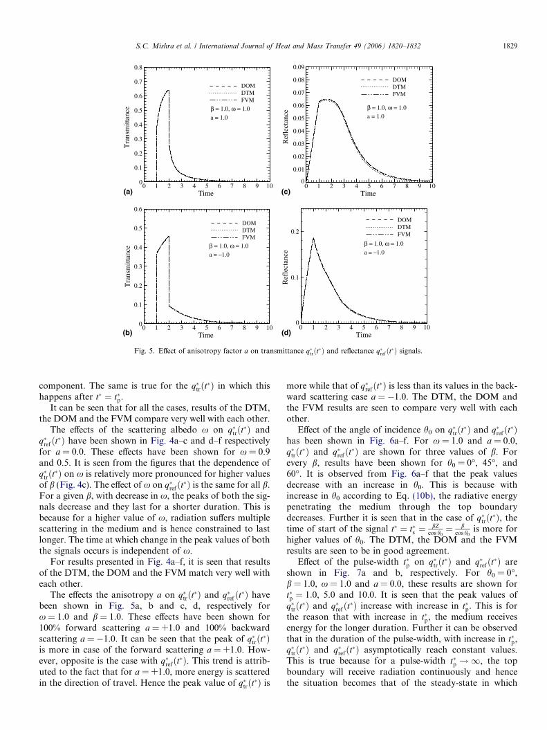
The effects the anisotropy a on q�trðt�Þ and q�refðt�Þ havebeen shown in Fig. 5a, b and c, d, respectively forx = 1.0 and b = 1.0. These effects have been shown for100% forward scattering a = +1.0 and 100% backwardscattering a = �1.0. It can be seen that the peak of q�trðt�Þis more in case of the forward scattering a = +1.0. How-ever, opposite is the case with q�refðt�Þ. This trend is attrib-uted to the fact that for a = +1.0, more energy is scatteredin the direction of travel. Hence the peak value of q�trðt�Þ is

more while that of q�refðt�Þ is less than its values in the back-ward scattering case a = �1.0. The DTM, the DOM andthe FVM results are seen to compare very well with eachother.

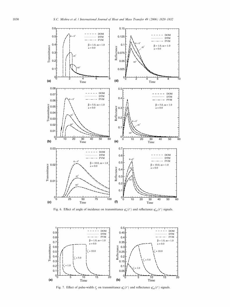
Effect of the angle of incidence h0 on q�trðt�Þ and q�refðt�Þhas been shown in Fig. 6a–f. For x = 1.0 and a = 0.0,q�trðt�Þ and q�refðt�Þ are shown for three values of b. Forevery b, results have been shown for h0 = 0�, 45�, and60�. It is observed from Fig. 6a–f that the peak valuesdecrease with an increase in h0. This is because withincrease in h0 according to Eq. (10b), the radiative energypenetrating the medium through the top boundarydecreases. Further it is seen that in the case of q�trðt�Þ, thetime of start of the signal t� ¼ t�s ¼ bZ

cos h0¼ b

cos h0is more for

higher values of h0. The DTM, the DOM and the FVMresults are seen to be in good agreement.

Effect of the pulse-width t�p on q�trðt�Þ and q�refðt�Þ areshown in Fig. 7a and b, respectively. For h0 = 0�,b = 1.0, x = 1.0 and a = 0.0, these results are shown fort�p ¼ 1:0, 5.0 and 10.0. It is seen that the peak values ofq�trðt�Þ and q�refðt�Þ increase with increase in t�p. This is forthe reason that with increase in t�p, the medium receivesenergy for the longer duration. Further it can be observedthat in the duration of the pulse-width, with increase in t�p,q�trðt�Þ and q�refðt�Þ asymptotically reach constant values.This is true because for a pulse-width t�p !1, the topboundary will receive radiation continuously and hencethe situation becomes that of the steady-state in which

Time

Tra

nsm

ittan

ce

0 2 4 6 80

0.1

0.2

0.3

0.4

0.5

0.6

DOMDTMFVM

45°

45°

45°

45°

45°

45°θ = 0°

θ = 0°

θ = 0°

θ = 0°θ =0°

θ = 0°

60°

60°

60°

60°

60°

60°

β = 1.0, ω = 1.0a = 0.0

β = 5.0, ω = 1.0a = 0.0

β = 10.0, ω = 1.0a = 0.0 β = 10.0, ω = 1.0

a = 0.0

β = 5.0, ω = 1.0a = 0.0

β = 1.0, ω = 1.0a = 0.0

Time

Ref

lect

ance

0 2 4 6 8 100

0.025

0.05

0.075

0.1

0.125

0.15

DOMDTMFVM

(a) (d)

Time

Tra

nsm

ittan

ce

0 10 20 30 40 50 600

0.01

0.02

0.03

0.04

0.05

0.06

0.07

0.08

DOMDTMFVM

Time

Ref

lect

ance

0 10 20 30 40 50 600

0.1

0.2

0.3

0.4

0.5

DOMDTMFVM

(b) (e)

Time

Tra

nsm

ittan

ce

0 25 50 75 1000

0.01

0.02

0.03DOMDTMFVM

Time

Ref

lect

ance

0 10 20 30 40 50 600

0.1

0.2

0.3

0.4

0.5

0.6

0.7

DOMDTMFVM

(c) (f)

Fig. 6. Effect of angle of incidence on transmittance q�trðt�Þ and reflectance q�ref ðt�Þ signals.

Time

Tra

nsm

ittan

ce

0 5 10 15 200

0.1

0.2

0.3

0.4

0.5

0.6

0.7

0.8

0.9

1DOMDTMFVM

tp* = 10.0

tp* = 5.0

tp* = 1.0

Time

Ref

lect

ance

0 5 10 15 200

0.05

0.1

0.15

0.2

0.25

0.3

0.35

0.4

0.45

0.5DOMDTMFVM

β = 1.0, ω = 1.0a = 0.0

β = 1.0, ω = 1.0a = 0.0

tp* = 10.0

tp* = 5.0

(a) (b)

tp = 1.0*

Fig. 7. Effect of pulse-width t�p on transmittance q�trðt�Þ and reflectance q�refðt�Þ signals.

1830 S.C. Mishra et al. / International Journal of Heat and Mass Transfer 49 (2006) 1820–1832

Table 1Comparison of the CPU times (in second) of the DTM, the DOM and theFVM

Number ofcontrol volumes

Numberof rays

CPU times (s)

DTM DOM FVM

100 40 165.31 85.67 155.80200 40 529.39 201.02 352.94300 40 605.22 381.19 486.31400 40 840.40 465.77 773.91500 40 959.38 620.00 923.00

500 10 537.29 328.97 380.91500 20 612.16 448.89 550.80500 30 809.84 517.92 750.70500 45 1056.83 724.66 939.19

S.C. Mishra et al. / International Journal of Heat and Mass Transfer 49 (2006) 1820–1832 1831

q�trðt�Þ and q�refðt�Þ will have constant values. In this casealso, the DTM, the DOM and the FVM results have a closematch.

3.1. Comparison of CPU times

Having found that in all the cases, the DTM, the DOMand the FVM results are in good agreement with eachother, we next study the computational efficiency of thethree methods. For b = 1.0, x = 1.0, a = 0.0 and h0 = 0�,the CPU times (in second) in the three methods are com-pared in Table 1. All runs were taken on the IBM Think-pad, Model R40, Mobile Intel Pentium 4, 2.0 GHz, 256MB RAM at 266 MHz.

It is seen from Table 1 that the DOM is computationallythe most efficient. Since the FVM and the DOM proce-dures are exactly the same, except that the FVM spendsextra time in integrating intensity over an elemental solidangle, the CPU time of the FVM is always higher thanthe DOM. However, this extra computation in the FVMhas an advantage over the DOM in multidimensionalgeometries and in strongly anisotropically scattering med-ium in which case the ray effect is more pronounced [36]The DTM spends much time in ray tracing and source termevaluation, hence its computational time is always morethan the DOM and the FVM.

4. Conclusions

A general formulation of the DTM, the DOM and theFVM to study the transmittance and reflectance signalscaused by the irradiation of a short-pulse laser was pre-sented. The formulations in the three methods were similarin the sense that the intensity directions and the quadra-tures to compute incident radiation and heat flux werethe same. The time marching procedure in the three meth-ods was also the same. The DTM differed from the DOMand the FVM in the ray tracing approach. To validate theformulation and to compare the results of the three meth-ods, a planar absorbing-scattering cold medium with blackboundary was considered. The transmittance and reflec-tance signals were studied and compared for different val-

ues of the extinction coefficient, the scattering albedo, theanisotropy factor, the angle of incidence and the pulse-width of the square pulse. These parameters were foundto have significant bearings on the temporal variations ofthese signals. In all the cases, the results from the threemethods were found to match very well with each other.Computationally, the DOM was found to be the mostefficient.

References

[1] M.J.C. Gemert, J.J. Wetch, Clinical use of laser–tissue interaction,JEEE Eng. Med. Biol. Mag. 8 (4) (1989) 10–13.

[2] F. Liu, K.M. Yoo, R.R. Alfano, Ultra-fast laser pulse transmissionand imaging through biological tissues, Appl. Opt. 32 (1993) 554–558.

[3] Y. Yamada, Light–Tissue Interaction and Optical Imaging in Bio-Medicine, vol. 6, Beggel House, New York, 1995, pp. 1–59.

[4] M. Sakami, K. Mitra, T. Vo-Dinh, Analysis of short-pulse laserphoton transport through tissues for optical tomography, Opt. Lett.27 (2002) 336–338.

[5] R.E. Walker, J.W. Mclean, Lidar equation for turbid media withpulse stretching, Appl. Opt. 38 (1999) 2384–2397.

[6] K. Mitra, J.H. Churnside, Transient radiative transfer equationapplied to oceanographic lidar, Appl. Opt. 38 (1999) 889–895.

[7] S.A. Prahl, M.J.C. Van Gemert, A.J. Welch, Determining the opticalproperties of turbid media by adding-doubling method, Appl. Opt. 32(1993) 559–568.

[8] J. Noack, A. Vogel, Single-shot spatially resolved characterization oflaser induced shock waves in water, Appl. Opt. 37 (1998) 4092–4099.

[9] C.L. Tien, A. Majumdar, F.M. Gerner, Microscale Energy Transfer,Taylor and Francis, Washington, DC, 1997.

[10] S. Kumar, K. Mitra, Microscale aspects of thermal radiationtransport and laser applications, Adv. Heat Transfer 33 (1999) 187–294.

[11] K.J. Grant, J.A. Piper, D.J. Ramsay, K.L. Williams, Pulse lasers inparticle detection and sizing, Appl. Opt. 33 (1993) 416–417.

[12] M.F. Modest, Radiative Heat Transfer, second ed., Academic Press,New York, 2003.

[13] R. Siegel, J. Howell, Thermal Radiation Heat Transfer, fourth ed.,Taylor & Francis, New York, 2002.

[14] N.G. Shah, A new method of computation of radiation heat transferin combustion chambers, Ph.D. Thesis, Imperial College, Universityof London, England, 1979.

[15] W.A. Fiveland, Discrete-ordinates solution of the radiative transportequation for rectangular enclosures, J. Heat Transfer 106 (1984) 699–706.

[16] J.C. Chai, S.V. Patankar, Finite volume method for radiation heattransfer, Adv. Numer. Heat Transfer 2 (2000) 110–135.

[17] S. Kumar, K. Mitra, Y. Yamada, Hyperbolic damped-wave modelsfor transient light-pulse propagation in scattering media, Appl. Opt.35 (1996) 3372–3378.

[18] K. Mitra, M.S. Lai, S. Kumar, Transient radiation transport inparticipating media within a rectangular enclosure, J. Thermophys.Heat Transfer 11 (1997) 409–414.

[19] Z.M. Tan, P.F. Hsu, An integral formulation of transient radiativetransfer, J. Heat Transfer 123 (2001) 466–475.

[20] Z.M. Tan, P.-f. Hsu, Transient radiative transfer in three-dimensionalhomogeneous and non homogeneous participating media, J. Quant.Spectros. Radiat. Transfer 73 (2002) 181–194.

[21] C.Y. Wu, S.H. Wu, Integral equation formulation for transientradiative transfer in an anisotropically scattering medium, Int. J. HeatMass Transfer 122 (2000) 818–822.

[22] C.Y. Wu, N.R. Ou, Differential approximation for transient radiativetransfer through a participating medium exposed to collimatedradiation, J. Quant. Spectros. Radiat. Transfer 73 (2002) 111–120.

1832 S.C. Mishra et al. / International Journal of Heat and Mass Transfer 49 (2006) 1820–1832

[23] H. Schweiger, A. Oliva, M. Costa, C.D.P. Segarra, A Monte Carlomethod for the simulation of transient radiation heat transfer:application to compound honeycomb transparent insulation, Numer.Heat Transfer B 35 (2001) 113–136.

[24] Z. Guo, J. Aber, B.A. Garetz, S. Kumar, Monte Carlo simulation andexperiments of pulsed radiative transfer, J. Quant. Spectros. Radiat.Transfer 73 (2002) 159–168.

[25] Z. Guo, S. Kumar, K.C. San, Multi-dimensional Monte Carlosimulation of short-pulsed transport in scattering media, J. Thermo-phys. Heat Transfer 14 (2000) 504–511.

[26] Z. Guo, S. Kumar, Discrete-ordinates solution of short-pulsed lasertransport in two-dimensional turbid media, Appl. Opt. 40 (2001)3156–3163.

[27] M. Sakami, K. Mitra, P.-f. Hsu, Analysis of light-pulse transportthrough two-dimensional scattering and absorbing media, J. Quant.Spectros. Radiat. Transfer 73 (2002) 169–179.

[28] Z. Guo, S. Kumar, Three-dimensional discrete ordinates method intransient radiative transfer, J. Thermophys. Heat Transfer 16 (2002)289–296.

[29] P. Rath, S.C. Mishra, P. Mahanta, U.K. Saha, K. Mitra, Discretetransfer method applied to transient radiative problems in partici-pating medium, Numer. Heat Transfer, Part A 44 (2003) 183–197.

[30] Z. Guo, S. Kumar, Radiation element method for hyperbolicradiative transfer in plane—parallel inhomogeneous media, Numer.Heat Transfer B 39 (4) (2001) 371–387.

[31] J.C. Chai, One-dimensional transient radiative heat transfer modelingusing a finite volume method, Numer. Heat Transfer B 44 (2003) 187–208.

[32] J.C. Chai, P.-f. Hsu, Y.C. Lam, Three-dimensional transient radiativetransfer modeling using the finite volume method, J. Quant. Spectros.Radiat. Transfer 86 (2004) 299–313.

[33] K. Mitra, S. Kumar, Development and comparisons of models forlight-pulse transport through scattering-absorbing media, Appl. Opt.38 (1999) 188–196.

[34] S.C. Mishra, H.K. Roy, N. Misra, Discrete ordinate method with anew and a simple quadrature scheme, J. Quant. Spectros. Radiat.Transfer, in press, doi:10.1016/j.jqsrt.2005.11.018.

[35] S.C. Mishra, P. Talukdar, D. Trimis, F. Durst, Computationalefficiency improvements of the radiative transfer problems with orwithout conduction—a comparison of the collapsed dimensionmethod and the discrete transfer method, Int. J. Heat Mass Transfer46 (2003) 3083–3095.

[36] P.J. Coelho, M.G. Carvalho, A conservative formulation of thediscrete transfer method, J. Heat Transfer 119 (1997) 118–128.