Development and test of a controlled source MT method in ... · of a controlled source MT method in...

Development and test of a controlled source MT method

in the frequency range 1 to 50 kHz

Andreas Pfaffhuber

Diploma ThesisJanuary 2001

Technical University BerlinInstitute for Applied Geoscience IIDepartment of Applied Geophysics

Ackerstraße 71-7613355 Berlin

ContentContentContentContentPrefacePrefacePrefacePreface 6666

IntroductionIntroductionIntroductionIntroduction 7777

1 Theory

1.1 Radiomagnetotelluric (RMT) 10

1.1.1 Basic principles1.1.1 Basic principles1.1.1 Basic principles1.1.1 Basic principles----------------------------------------------------------------------------------------------------------------------------------------------------------------------------------------------------------------------------------------------------------------------------------------------------10101010

1.1.2 The impedance tensor in controlled source RMT (CSRMT)1.1.2 The impedance tensor in controlled source RMT (CSRMT)1.1.2 The impedance tensor in controlled source RMT (CSRMT)1.1.2 The impedance tensor in controlled source RMT (CSRMT)------------------------------------------------------------------------------------12121212

1.1.3 The magnetotelluric formulation of a 1D earth1.1.3 The magnetotelluric formulation of a 1D earth1.1.3 The magnetotelluric formulation of a 1D earth1.1.3 The magnetotelluric formulation of a 1D earth------------------------------------------------------------------------------------------------------------------------------------------------13131313

1.2 Finite sources over a layered halfspace 14

1.2.1 Reflection coefficients1.2.1 Reflection coefficients1.2.1 Reflection coefficients1.2.1 Reflection coefficients--------------------------------------------------------------------------------------------------------------------------------------------------------------------------------------------------------------------------------------------------------------------14141414

1.2.2 Horizontal magnetic dipole1.2.2 Horizontal magnetic dipole1.2.2 Horizontal magnetic dipole1.2.2 Horizontal magnetic dipole----------------------------------------------------------------------------------------------------------------------------------------------------------------------------------------------------------------------------------------15151515

General solution 16Far field approximation 17Near field approximation 18

2 Modeling

2.1 Numerical realization 20

2.1.1 Digital filtering2.1.1 Digital filtering2.1.1 Digital filtering2.1.1 Digital filtering------------------------------------------------------------------------------------------------------------------------------------------------------------------------------------------------------------------------------------------------------------------------------------------------------------20202020

2.1.2 Computing the CSRMT Impedance tensor2.1.2 Computing the CSRMT Impedance tensor2.1.2 Computing the CSRMT Impedance tensor2.1.2 Computing the CSRMT Impedance tensor--------------------------------------------------------------------------------------------------------------------------------------------------------------------21212121

2.1.3 Far field estimation2.1.3 Far field estimation2.1.3 Far field estimation2.1.3 Far field estimation------------------------------------------------------------------------------------------------------------------------------------------------------------------------------------------------------------------------------------------------------------------------------------23232323

2.2 Homogeneous halfspace 24

2.2.1 Comparison of the far field approximation and the general solution2.2.1 Comparison of the far field approximation and the general solution2.2.1 Comparison of the far field approximation and the general solution2.2.1 Comparison of the far field approximation and the general solution------------------------------------24242424

2.2.2 Fields over a homogeneous halfspace2.2.2 Fields over a homogeneous halfspace2.2.2 Fields over a homogeneous halfspace2.2.2 Fields over a homogeneous halfspace------------------------------------------------------------------------------------------------------------------------------------------------------------------------------------26262626

Amplitudes 27Phases 30

2.2.3 Scalar resistivities2.2.3 Scalar resistivities2.2.3 Scalar resistivities2.2.3 Scalar resistivities--------------------------------------------------------------------------------------------------------------------------------------------------------------------------------------------------------------------------------------------------------------------------------------------31313131

2.2.4 RMT tensor resistivities2.2.4 RMT tensor resistivities2.2.4 RMT tensor resistivities2.2.4 RMT tensor resistivities--------------------------------------------------------------------------------------------------------------------------------------------------------------------------------------------------------------------------------------------------------------------32323232

Dependency on position 32Dependency on frequency and resistivity 35

2.3 Two layer case 36

2.3.1 Conductive overburden2.3.1 Conductive overburden2.3.1 Conductive overburden2.3.1 Conductive overburden--------------------------------------------------------------------------------------------------------------------------------------------------------------------------------------------------------------------------------------------------------36363636

2.3.2 Resistive overburden2.3.2 Resistive overburden2.3.2 Resistive overburden2.3.2 Resistive overburden------------------------------------------------------------------------------------------------------------------------------------------------------------------------------------------------------------------------------------------------------------------------37373737

-2-

2.3.3 Dependency on resistivity contrast2.3.3 Dependency on resistivity contrast2.3.3 Dependency on resistivity contrast2.3.3 Dependency on resistivity contrast----------------------------------------------------------------------------------------------------------------------------------------------------------------------------------------------------38383838

2.4 Far field distance estimation 40

2.5 Summary of the modeling results 43

3 Instrument

3.1 Receiver 45

3.1.1 Technical specification3.1.1 Technical specification3.1.1 Technical specification3.1.1 Technical specification----------------------------------------------------------------------------------------------------------------------------------------------------------------------------------------------------------------------------------------------------------------45454545

3.1.2 The control panel3.1.2 The control panel3.1.2 The control panel3.1.2 The control panel----------------------------------------------------------------------------------------------------------------------------------------------------------------------------------------------------------------------------------------------------------------------------------------47474747

3.2 Transmitter 51

3.2.1 Technical description3.2.1 Technical description3.2.1 Technical description3.2.1 Technical description------------------------------------------------------------------------------------------------------------------------------------------------------------------------------------------------------------------------------------------------------------------------51515151

3.2.2 Improvements3.2.2 Improvements3.2.2 Improvements3.2.2 Improvements--------------------------------------------------------------------------------------------------------------------------------------------------------------------------------------------------------------------------------------------------------------------------------------------------------52525252

Power supply 53Heat production 53

4 Measurements

4.1 Laboratory 56

4.1.1 Transmitter output4.1.1 Transmitter output4.1.1 Transmitter output4.1.1 Transmitter output----------------------------------------------------------------------------------------------------------------------------------------------------------------------------------------------------------------------------------------------------------------------------------------56565656

4.1.2 Calibration4.1.2 Calibration4.1.2 Calibration4.1.2 Calibration----------------------------------------------------------------------------------------------------------------------------------------------------------------------------------------------------------------------------------------------------------------------------------------------------------------------------57575757

4.1.3 Control program verification4.1.3 Control program verification4.1.3 Control program verification4.1.3 Control program verification----------------------------------------------------------------------------------------------------------------------------------------------------------------------------------------------------------------------------------------58585858

4.2 Field 59

4.2.1 Resonance curves4.2.1 Resonance curves4.2.1 Resonance curves4.2.1 Resonance curves----------------------------------------------------------------------------------------------------------------------------------------------------------------------------------------------------------------------------------------------------------------------------------------59595959

4.2.2 Transmitter currents4.2.2 Transmitter currents4.2.2 Transmitter currents4.2.2 Transmitter currents--------------------------------------------------------------------------------------------------------------------------------------------------------------------------------------------------------------------------------------------------------------------------------60606060

4.2.3 Received signals4.2.3 Received signals4.2.3 Received signals4.2.3 Received signals------------------------------------------------------------------------------------------------------------------------------------------------------------------------------------------------------------------------------------------------------------------------------------------------60606060

5 Interpretation concepts

5.1 Inversion of near field data 63

5.2 Joint CSRMT and VLF profiling 65

6 Conclusion and Outlook

AcknowledgmentsAcknowledgmentsAcknowledgmentsAcknowledgments 69696969

List of figuresList of figuresList of figuresList of figures 70707070

AppendixAppendixAppendixAppendix 73737373

-3-

Symbols

The most important symbols are listed and explained below. Generally boldletters mark vectors, underlined bold letters stand for tensors. Capital letters markthe frequency space whereas the lower case indicates the time space.

Coordinate system:

x,y,z cartesian coordinates m,m,mr,ϕ,z cylindrical coordinates m,rad,m∪ kx

2≤k y

2 wavenumber 1/mt time sω angular frequency rad/s

Fields and related quantities:E,e ... electric field intensity V/mJ∪ᵀ E ... electric current density A/m²D∪E ... dielectric displacement C/m²H,h ... magnetic field intensity A/mB∪H ... magnetic induction Tesla

Z∪Ex

H y∪≥

E y

H x ... scalar impedance m/s

Z E∪Z«H ... impedance tensor m/sT ... tipper vector

p∪ 2ᵀ

... skin depth m

Material properties and their derivatives:

∪ᵀ≥1 ... electric resistivity Ωm

ω ... dielectric permittivity C/Vm ... magnetic permeability Vs/Am

z∪ j ... impedivityy∪ᵀ≤ j ... admittivityk∪ ≥z y ... complex wavenumberkᵀ∪ jᵀ ... k for the quasi static approximation

-4-

Parameters of the layered halfspace

Zi∪zki

... impedance of the ith layer m/s

Zi ... impedance at the top of the ith layer m/s

Y i∪1Zi

admittance of the ith layer s/m

Y i ... admittance at the top of the ith layer s/mrTE ... reflection coefficient for TE moderTM ... reflection coefficient for TM mode

Source related quantities

Az ... scalar TM potential of the HMDFz ... scalar TE potential of the HMDJ0,1 ... Bessel function of order 0,1 of the first kindm ... magnetic moment of the loop Am²h ... height of the source dipole axis m

x5° ... FFD in x- direction at 5° phase deviation my10 ... FFD in y- direction at 10 % ampl. deviation m

-5-

Preface

This thesis represents the final work of my studies at the Department of AppliedGeophysics at the Technical University Berlin. With this, I am finishing my courseof studies titled “Applied Geoscience” majoring Applied Geophysics.The relatively new course of studies, “Applied Geoscience” combines a broadgeoscientific background (which I gathered at the Mining University Leoben,Austria) with a profound knowledge of the specific main subject. Especially forgeophysicists it is important to understand and question the geological plausibilityof the various processing results of acquired field data.During my studies in Berlin I was involved in a scientific project work of Tino Radicand Prof. Hans Burkhardt. The aim of this project was to evaluate the applicabilityof high temperature SQUID magnetometers for geophysical applications. In thescope of this project a new radio-frequency magnetotelluric (RMT) instrument wasdesigned. As the Metronix company was a partner of the project, a transmitterwith a frequency range from 1 kHz and upwards was contributed by them. As aresult of the limited length of time, this transmitter prototype was never usedduring the project. Due to the lower applicable frequencies, the transmitterenables deeper soundings as the depth of investigation is inversely proportionalto the square root of the frequency. Hence, this would increase the field ofpossible applications reaching deeper structures. However, before starting anyfield measurements, it has to be investigated if approximations, used in similarmethods can be applied. For example if or under which restrictions assumptionscan be adapted, that are used for conventional magnetotelluric processing.Induced by all these facts, step by step the main topic for my diploma thesisarose.After the project was finished, I started to rework the transmitter to a field suitablecondition. The control program of the RMT receiver also had to be adapted tomeet the new requirements. At the same time I developed a forward modelingprogram for the fields of the used horizontal magnetic dipole (HMD) source.

-6-

Introduction

The radio-frequency magnetotelluric or radiomagnetotelluric (RMT) method,introduced by Turberg et. al. (1994), uses the electric and magnetic fields ofartificial transmitters far off the measuring site in the frequency range from about16 kHz up to 240 kHz. These sources are powerful communication transmittersfor submarines in the very low frequency range (VLF) from 10 to 30 kHz and radiotransmitters at higher frequencies. Hence, RMT is an extension to higherfrequencies of the VLF-R technique described by McNeill and Labson (1988).Using standard MT algorithms, it is possible to estimate the apparent resistivity ofthe subsurface from orthogonal horizontal electric and magnetic fields on theearth's surface (Ward and Hohmann, 1988).The typical fields of application are environmental problems such as the mappingof lateral and vertical boundaries of waste disposal sites (Tezkan et. al., 1995)and hydrogeophysical topics (Turberg et. al., 1994). With the five channel RMTinstrument, developed at the department of Applied Geophysics (Radic andBurkhardt, 2000), it is possible to acquire resistivity data in a fast manner, whichmakes the system attractive for all types of resistivity profiling and sounding. Withthe introduced instrument it is possible to work with frequencies up to 1 MHz.A limitation of the method is the frequency range and therefore the depth ofinvestigation, as the lowest frequency and the resistivity of the subsurfacedetermines the penetration depth of the electromagnetic waves. Regarding thisproblem, Tezkan et. al. (1995) combined transient electromagneticmeasurements with RMT soundings to increase the depth of exploration. Anotherapproach to overcome this limitation is the introduction of a transmitter to thesystem, extending the frequency range to lower limits. Furthermore in rural areas,where no radio transmitters are close, a controlled source contributes the neededsignal strength. In contrast to RMT, for the audio frequency range the applicationof a horizontal electric dipole as source is a conventional method these days,called controlled source audiomagnetotelluric (CSAMT, Zonge and Hughes,1988). Regarding AMT, the introduction of a transmitter was mainly due to theinstable and often weak natural signals in this frequency range. As source forRMT the concept of a horizontal magnetic dipole (HMD) is prefered. This dipoletype is realized by vertikal standing loops in the field. The Metronix companycontributed a RMT transmitter to the department of Applied Geophysics during ajoint project. This source is a prototype of a later developed transmitter for theEnviroMT system, designed by the University of Uppsala (Sweden) and Metronix(Pedersen et. al., 1999).

This thesis illustrates the development of a CSRMT system from the five channelRMT receiver and the transmitter prototype. Besides the reworking of theinstrument and its controlling software, synthetic data were calculated to evaluatethe applicability of the plane wave solution (or to say MT interpretation) on theCSRMT measurements.In the first chapter of this work the theoretical background for electromagneticfields interacting with conductive matter is given. The description of the sourcefields, both with a general formula and approximations for the near and far field isof special interest.

-7-

The results of the modeling are illustrated in the second chapter. Amplitude andphase of the electric and magnetic fields of the HMD as well as the regardingmagnetotelluric (scalar and tensor resistivities) and magnetic (tipper vector)transfer functions are presented. They are calculated considering the frequency,position of the receiver and subsurface resistivity. To evaluate the satisfaction ofthe far field condition, the synthetic data are compared to the MT apparentresistivities of the model. Resting upon the deviation of the HMD- and MTapparent resistivities, the far field distance (FFD) is introduced. It marks the rangebetween transmitter and receiver where the deviation drops below a certain value.Besides a homogeneous halfspace, several two layer cases with differentresistivity contrasts are taken into account to study the dependency of the FFD onthe contrast. Finally a field formula to estimate the FFD is developed, whichrelates the far field distance to the skin depth.In chapter three the changes that were adapted to the transmitter prototype andthe RMT receiver control program are listed and described.Chapter four illustrates the measurements performed both in the field andlaboratory. Before any field measurements were started, the power of thetransmitter amplifier was checked in the office. To verify all realized changes onthe receiver system, it was calibrated and a simulation of a field measurementwas conducted in the laboratory. Most of the field days were invested in testsrelated to the reworking of the transmitter. Hence, some acquired resonancecurves are shown. To evaluate the actual transmitter moments for the specificfrequencies, the maximum achievable currents in the transmitter loop wereacquired under field conditions as well. Amplitudes of acquired fields arecompared with synthetic data to end the measurements chapter.Just previous to the conclusion, in chapter five two interpretation concepts,considering the results of the modelings and measurements, are introduced.

-8-

1 Theory

-9-

Chapter: Theory 1.1 Radiomagnetotelluric (RMT)

1.1 Radiomagnetotelluric (RMT)

Magnetotelluric (MT) deals with magnetic and electric fields on the earth's surfaceto investigate the conductivity structure of the subsurface. The origins of these electromagnetic (EM) fields are sources on or above theearth's surface on one, and induced (secondary, internal) fields on the other side.Primary source fields are also called fields of external origin. These natural orartificial fields appear as homogeneous (plane waves) or inhomogeneous,spatially deformed fields around a finite source. In the so called far fieldinhomogeneous source fields can be treated as plane waves. The electrical resistivity of the earth determines the secondary field strength andpolarization which makes it possible to extract the subsurface resistivityinformation from the measured field data. The following chapters will show the physical background for the oncoming topics.In the first subchapter some general descriptions of plane wave fields are given.The second subchapter gives the theoretical background for spatial deformedsource fields of finite source.Radiomagnetotelluric systems work on the MT-principle in the frequency rangefrom 1 kHz up to 1 MHz. Sources of the electromagnetic fields are powerfulcommunication transmitters for submarines in the VLF-frequency range (10-30kHz) and radio transmitters at higher frequencies. Hence the basic relations forMT are given.

1.1.1 1.1.1 1.1.1 1.1.1 Basic principlesBasic principlesBasic principlesBasic principles

The following derivations are taken from Ward and Hohmann (1988) when no other source is given. Working with time-varying fields e , h∪e0 , h0 e j t in homogeneous regions andtaking the constitutive relations B∪H , J∪ᵀ E , D∪E (with electricalproperties which are independent of time, temperature and pressure and µassumed to be that of free space) into account, the Maxwell equations in thefrequency domain are

E≤z H ∪0H≥ y E∪0 (1-1)

with the impedivity z∪ j and the admittivity y∪ᵀ≤ jω . Considering planewaves traveling in z- direction the Maxwell equations can be converted into waveequations respectively Helmholtz equations in E and H

2 E≤k2 E∪0

2 H ≤k2 H ∪0(1-2)

where k is the complex wave number k2∪≥z y∪2≥ jᵀ .

-10-


The solutions of the wave equation for a sinusoidal time dependence are

e∪e0 e≥ j kz≥ t

h∪h0 e≥ j kz≥ t . (1-3)

Equations (1-3) describe a wave varying sinusoidally with z and t. As one can seethe imaginary part of k attenuates the wave in z- direction. The distance at whichthe amplitude is reduced by a factor of 1/e is called the skin depth p, where

p∪ 2ᵀ

. (1-4)

Employing the solutions (1-3) into the first Maxwell equation (1-1a) andconsidering waves polarized in the xy- plane, one will get the followingrelationship:

Ex

H y∪≥

E y

H x∪

k∪Z (1-5)

In this equation Z stands for the plane wave impedance which is themagnetotelluric transfer function, defined as the ratio of orthogonal horizontalelectric and magnetic field pairs. As ω2

∈ jᵀ ∀ k2∋ jᵀ ∪k

ᵀ

2 for earthmaterials at frequencies less than 100 kHz equation (1-5) can be rewritten as

Z∪

kᵀ

δ ΣΣ∪1

ΣZΣ2 (1-6)

Equation (1-6) is valid over a 1D earth which is never the case in practice.Reflection and refraction of plane EM waves on two- or three-dimensional bodiesresult in a tensor definition of the impedance.

Z∪Zxx Zxy

Z yx Z yy ∀ E∪Z«H (1-7)

Over a 1D earth Zxy = - Zyx and Zxx , Zyy = 0.

-11-


In 2- and 3D environments an additional parameter besides the impedance tensoris used. The so called tipper vector T, which is the vertical magnetic transferfunction, describing the relationship between the horizontal and the verticalmagnetic fields. It is defined as

H z∪T x H x≤T y H y , T∪T x T yT . (1-8)

For a horizontally layered halfspace T = 0 due to Hz = 0. In the 2D case T ≠ 0 in theTE mode which means that the polarization of the electric field is parallel to thegeological strike. If the E fields are normal to it and the magnetic fieldcomponents are parallel to the strike the fields are of TM mode. TE and TM modeare notations which are used in MT literature. However, the given description forthe two modes exactly meets the definition of the E- respectively B-polarization.To be strictly correct, TE mode means that the electric field is tangential to thesurface and therefore has no vertical component. The correct definition of the TMmode follows analogically.

1.1.2 1.1.2 1.1.2 1.1.2 The impedance tensor in controlled source RMT (CSRMT)The impedance tensor in controlled source RMT (CSRMT)The impedance tensor in controlled source RMT (CSRMT)The impedance tensor in controlled source RMT (CSRMT)See Zonge and Hughes (1988) for more details on this topic

The natural signal sources in MT have an infinite number of polarizations. Henceall elements of the impedance tensor and tipper vector can be estimated formone measurement of Ex, Ey, Hx, Hy and Hz. Artificial signals have one finite locationand polarization which makes it impossible to determine the tensor elements fromone measurement. Two independent, preferably perpendicular sourcepolarizations must be used to calculate all of them. Since Z has to meet E1 = Z H1

as well as E2 = Z H2 where the subscripts 1 and 2 indicate the two different sourcepolarization, Z can be calculated by

Zxx∪Ex1 H y2≥Ex2 H y1

H x1 H y2≥H x2 H y1

, (1-9)

Zxy∪Ex2 H x1≥Ex1 H x2


, (1-10)

Z yx∪E y2 H y1≥E y1 H y2


, (1-11)

Z yy∪E y1 H x2≥E y2 H x1


. (1-12)

In a similar way one can determine the tipper elements:

-12-


T x∪H z1 H x2≥H z2 H x1

H y1 H x2≥H x1 H y2(1-13)

T y∪H z2 H y1≥H z1 H y2

H y1 H x2≥H x1 H y2(1-14)

1.1.3 1.1.3 1.1.3 1.1.3 The magnetotelluric formulation of a 1D earthThe magnetotelluric formulation of a 1D earthThe magnetotelluric formulation of a 1D earthThe magnetotelluric formulation of a 1D earthThe following considerations are taken from Ward and Hohmann (1988)

Performing MT measurements over a homogeneous halfspace yields directly thetrue electric conductivity of the subsurface using equation (1-6). Considering a horizontally layered halfspace changes this relation. Layeredmeans that the electrical parameters of the material change only along the z axis.Properties change at boundaries and are homogeneous within each layer.Measurements over such a 1D earth yield an apparent resistivity, named MTapparent resistivity in the following, which is affected by all layers.To determine the impedance of this layered earth, in each layer up- and down-traveling waves are considered. Implying the continuity of tangential fields acrossinterfaces leads to a recursive formulation of the plane wave impedance of a n-layered isotropic earth:

Zn∪Zn

Zn≤1≤Zn tanh j kn hn

Zn≤ Zn≤1 tanh j kn hn n∪1,2,..,N≥1 (1-15)

The corresponding earth model consists of N-1 layers of thickness hn, lying overan uniform halfspace. Zn is the intrinsic impedance of every strata after equation(1-5), whereas Zn denotes the impedance at the top of the nth layer derived byequation (1-15), except for the underlying halfspace where Z N∪Z N . Usingequation (1-15) it is easy to compute Z1 and the MT apparent resistivityrespectively. The surface admittance Y 1

can be calculated analogically wherebythe intrinsic admittance is given as Y n∪k ≠ z .

-13-

Chapter: Theory 1.2 Finite sources over a layered halfspace

1.2 Finite sources over a layered halfspace

Fields of an finite electromagnetic source on or over a conducting halfspace canbe expressed as a superposition of numerous reflected plane waves at differentangles of incidence.As expected these fields don't satisfy the plane wave approximations of equation(1-2) within a certain distance from the source. This region is called “near field”.Further away, in the “far field” the fields comply with the properties of normalincident plane waves.

1.2.1 1.2.1 1.2.1 1.2.1 Reflection coefficientsReflection coefficientsReflection coefficientsReflection coefficients

To determine the fields of the source over a layered halfspace, reflection andrefraction of the EM wave on the numerous boundaries must be considered.Developing Snell's laws and the Fresnel equations yields the reflectioncoefficients for E perpendicular to (TE) and in (TM) the plane of incidence (Wardand Hohmann, 1988, pp. 183-202). The reflection coefficients for the surface of the layered halfspace for TE and TMmode are given by

rTE∪Y 0≥ Y 1

Y 0≤ Y 1

and rTM∪Z0≥ Z1

Z0≤ Z1

. (1-16 a,b)

As rTM won't be used explicitly in the following, no simplifications are done on (1-16 b). In equation (1-16 a) Y0 stands for the free space admittance and Y 1

has tobe determined by

Y n∪Y n

Y n≤1≤Y n tanh un hn

Y n≤ Y n≤1 tanh un hn (1-17)

as Zn in equation (1-15). Instead of the complex wavenumber for normalincidence (k), oblique incidence is considered now with

un2∪kx

2≤k y

2≥kn

2∪

2≥kn

2 . (1-18)

Note that also for Y n∪un ≠ zn not k but u has to be taken into account. Settingzn∪z0 for a nonmagnetic structure Y n and Y n can be replaced by un and un in

equations (1-16) and (1-17).

-14-


Regarding the source field in free space the quasi static approximation is applied.Therefore the free space wavenumber k0 for low frequencies and equation(1-16) turns into

rTE∪≥u1

≤u1

. (1-19)

The complex wavenumber on the surface of a layered earth is given recursivelyas

un∪unun≤1≤un tanh un hn

un≤un≤1 tanh un hn . (1-20)

Note that the complex wavenumber kn in equation (1-18) contains ω, µ, σand ε aswell though displacement currents derived by ε0 are neglected in (1-19) for thefree space. Thus for the subsurface no low frequency approximation as inequation (1-6) was employed.

1.2.2 1.2.2 1.2.2 1.2.2 Horizontal magnetic dipoleHorizontal magnetic dipoleHorizontal magnetic dipoleHorizontal magnetic dipole

At a distance of at least 5 (Ward and Hohmann, 1988), better 10 (Dey and Ward,1970) loop radii a vertical loop can be treated as a horizontal dipole (HMD). In thefollowing considerations the dipole axis is aligned in x direction in a height of hmeters.The field of a horizontal magnetic dipole consists of TE and TM modes as there isboth an electric and a magnetic vertical field component. The TM and TEpotentials are given as (Ward and Hohmann, 1988)

Az r ,z∪≥k0

2 m4

ψ

ψ yˇ0

1≤rTM e≥u 0 h 1u0

J 0 rd ,

F z r ,z∪≥z0 m4

ψ

ψ xˇ0

1≤rTEe≥u 0 h 1

J 0 rd

(1-21)

where Az stands for the TM and Fz the TE potential. m represents the magneticmoment of the source in Am2 and J0 stands for the Bessel function of order 0 ofthe first kind. A cylindrical coordinate system is used with r∪ x2

≤ y2 and zpointing downwards. The fields can be derived from the potentials using

E∪≥z A≤ 1yν ν«A≥νF and

H∪≥y F≤1zν ν«F ≤νA .

(1-22)

-15-


General solution

Due to the infinite impedance contrast at the earth's surface and the inductivelycoupled source field, no TM mode fields are excited inside the conductive earth inthe scope of the quasi static approximation. This can be seen from equation (1-21), since for k0∋0 the TM mode potential for a 1D earth Az vanishes. Usingequations (1-22) on Fz yields after differentiation

H x∪m

42 x2

r 3 ≥1rI 1≥

x2

r 2 I 2 (1-23)

H y∪m

42xyr3 I 1≥

xyr2 I 2 (1-24)

H z∪≥m

4xr

I 3 (1-25)

Ex∪m

4i≥2xy

r3 I 4≤xyr2 I 5 (1-26)

E y∪m

4i2 x2

r 3 ≥1rI 4≤

x2

r2 I 5 (1-27)

where I 1∪ˇ0

1≥rTE e≥h J 1 rd ,

I 2∪ˇ0

1≥rTE e≥h 2 J 0 rd ,

I 3∪ˇ0

1≤rTE e≥h 2 J 1 rd ,

I 4∪ˇ0

1≤rTE e≥h J 1 rd and

I 5∪ˇ0

1≤rTE e≥h J 0 rd .

(1-28)

The vector components of the fields E and H are given in cartesian coordinates.In equations (1-23) to (1-24) r∪ x2

≤ y2 describes the distance betweentransmitter and receiver on the xy plane.

-16-


Far field approximation

At a transmitter – receiver separation of several skin depths ( k r∉1 ), the far fieldapproximation can be used to compute the fields of the source without solvingany Integrals resp. Hankel transforms. Since the Integrals in equation (1-28) showan asymptotical behavior for r δ the fields over a homogeneous halfspace withboth transmitter and receiver on the surface can be expressed as

H r∪m r31≥ 6

kᵀ

2 r2cos , (1-29)

H ∪m

2 r31≥ 3kᵀ

2 r2sin , (1-30)

H z∪≥3m

2 kᵀ

r4 cos , (1-31)

Er∪kᵀ

m2ᵀ r3 sin , (1-32)

E ∪≥kᵀ

mᵀ r3 cos , (1-33)

where kσ stands for the complex wavenumber for the low frequency approximationas in equation (1-6). Different from the general solution now the fields are given incylindrical components. Hr and Er stand for the radial components respectively Hϕ

and Eϕ for the tangential components (Weidelt, lecture script, unpublished).Calculating the apparent resistivity from orthogonal electric and magnetic fieldpairs as in equation (1-6) yields the MT apparent resistivity of the halfspace asthe terms in brackets in equations (1-29) and (1-30) tend to unity for k r∉1 .

-17-


Near field approximation

For comparison also the solutions for the near field valid if k r∈1 are given.

H r∪m

2 r3 cos , (1-34)

H ∪m

4 r3 sin , (1-35)

H z∪≥kᵀ

2 m16 r

cos , (1-36)

Er∪kᵀ

2 m4ᵀ r2 sin , (1-37)

Eᵀ∪≥

kᵀ

2 m4ᵀ r2 cos . (1-38)

-18-

2 Modeling

-19-

Chapter: Modeling 2.1 Numerical realization

2.1 Numerical realization

The forward modeling program CSRMT_1Dmod.llb was developed withLabVIEWTM 5.1, a graphical programming platform used in the completed projectin which the receiver and its controlling software was designed. Using the program it is possible to calculate the amplitudes and phases of Ex,y,Hx,y,z, Z, Z and T for a layered halfspace with intrinsic resistivity, thickness, anddielectric permittivity for each layer. Calculations can be done with respect toposition, frequency and transmitter height & moment. In addition there is thepossibility to determine a so called far field distance (FFD). At the FFD betweenreceiver and transmitter the deviation of the HMD apparent resistivity to the MTapparent resistivity of the model drops below a certain value. The HMD apparentresistivity is derived from the orthogonal horizontal electric and magnetic fields ofa HMD over a layered halfspace, calculated from equations (1-23) to (1-27). Forexample, the maximum deviation equals 10 % of the amplitude or 1° of the phase.In this work this is called far field estimation.

2.1.1 2.1.1 2.1.1 2.1.1 Digital filteringDigital filteringDigital filteringDigital filtering

To compute the numerous Hankel transforms in equations (1-28) a digital filterdeveloped by Guptasarma and Singh (1997) was used. They presented two filtersboth for the Hankel transforms of order 0 and 1 of first kind. In this work theshorter filters with 61 points for J0 resp. 47 points for J1 have been used.

The Integrals of the Hankel transforms are of the form

f r∪ˇ0

F J 0,1 rd . (2-1)

Substituting r∪ea and ∪e≥b in equation (2-1) leads to a convolution integral

r«f r∪≥

k bha≥bdb , (2-2)

with k b∪F as the input and ha≥b∪ r J 0,1 r as the filter function of thesystem. This integral can be approximated by the discrete convolution

r«f r∪i∪1

l

k r≥ihi . (2-3)

This numerical approach on analytically known Hankel transforms yields the filterfunction h(i) and the values for shift sh and spacing sp.

-20-


To perform the convolution, the kernel function F must be computed onspecific abscissa values λ i which are calculated with the help of sh and sp:

i∪1r

10sh≤i≥1 sp , i∪1,2,...,l . (2-4)

The integral can then be computed with

f r∪i∪1

l

F ihi

r

. (2-5)

The curves for hi and values for sh and sp are given in Appendix II÷1. Values for hi

are listed in Guptsarma and Singh (1997).

To investigate the accuracy ofthe digital filter routine, twoknown Hankel transforms werecomputed analytically and withthe filter algorithm. Oneexample for the order 0 is

ˇ0

e≥hJ 0rd∪ h

h2≤r2

3

and for the order 1

ˇ0

e≥hJ 1 rd∪ r

h2≤r2

3 .

Calculations were done for rfrom 0 to 1.000 m at a height h of 1.25 m. The deviation of the two single results isshown in figure 2-1 for both of the transforms. In the range of r, which is ofinterest, the deviation remains below 0.1 %. This accuracy meets therequirements for the forward modeling routine. Therefore the numerical approachis the basis of the further work.

2.1.2 2.1.2 2.1.2 2.1.2 Computing the CSRMT Impedance tensorComputing the CSRMT Impedance tensorComputing the CSRMT Impedance tensorComputing the CSRMT Impedance tensor

The fields E, H and Z are calculated directly from equations (1-23) to (1-27) and(1-5). To compute the elements of the impedance tensor, measurements with twotransmitter polarizations have to be considered. In order to keep the time forcalculation low, only one polarization is computed and afterwards rotated to asecond. This can be done, as long as a layered earth is concerned. For both

-21-

Figure 2-1 Deviation of the Hankel transformscomputed analytical and with a digital filter.

0 200 400 600 800 1000

1E-5

1E-4

1E-3

0.01

r [m]

Devia

tion

[%] e-λh λ J1(rλ)

e-λh λ J0(rλ)


polarizations the transmitter is located at (x=0 , y=0) with dipole axis x resp. y forpolarization 1 resp. 2. Relating the new coordinates (x2 , y2) to the original values(x1 , y1) is the first step to rotate the data matrix. In this case

x2∪≥ y1 , y2∪x1 (2-6)

and consequently the function values f for the 2nd polarization are

f 2x2 , y2∪ f 1 ≥ y1 , x1 . (2-7)

Next the changed directions of the calculated fields have to be considered afterequation (2-6). To give an example H x2 x2 , y2∪≥H y1 ≥ y1 , x1 . After equation (1-24) a changed sign of y also changes the sign of Hy. With f y1 , x1∪ f T

x1 , y1

the fields of the second polarization are

H x2∪H y1T , Ex2∪≥E y1

T ,H y2∪H x1

T , E y2∪≥Ex1T and

H z2∪H z1T .

(2-8)

Applying equations (2-8) on equations (1-9) to (1-14) yields

Zxx∪Ex1 H x1

T ≤E y1T H y1

H x1 H x1T ≥H y1

T H y1

, Zxy∪≥E y1

T H x1≥Ex1 H y1T

H x1 H x1T ≥H y1

T H y1

,

Z yx∪≥Ex1

T H y1≥E y1 H x1T

H y1T H y1≥H x1 H x1

T , Z yy∪E y1 H y1

T ≤Ex1T H x1

H y1T H y1≥H x1 H x1

T ,

T x∪H z1 H y1

T ≥H z1T H x1

H y1 H y1T ≥H x1 H x1

T , T y∪H z1

T H y1≥H z1 H x1T

H y1 H y1T ≥H x1 H x1

T .

(2-9)

In this way the impedance- and tipper elements are determined from one forwardmodeling.

-22-


2.1.3 2.1.3 2.1.3 2.1.3 Far field estimationFar field estimationFar field estimationFar field estimation

As mentioned before, the program is able to find the distance to the transmitterwhere the deviation of the HMD- to the MT apparent resistivities of the modeldrops below a certain value. Compared to the analytical far field conditionkr1 this way represents a more handsome definition of the far field which canbe used in the field as well. It can be calculated for certain frequencies andresistivities. The decisive condition for the far- / nearfield determination is thedeviation of the HMD- and MT apparent resistivity of the model.The distance is found easily: For a certain frequency and resistivity the searchroutine starts in the far field at a distance of 1.000 m which is decreased by a steplength of 50 m every iteration. As soon as the near field is reached, the steplength is reduced to 5 m and the current distance increased by 50 m to get intothe far field again. This procedure continues down to a step length of 0.1 m.Hence the far field estimation is computed with an accuracy of 0.1 m. Thecalculated FFDs are termed x1° or y5 which stands for a deviation of 1° phase or5 % amplitude respectively distances in x- or y- direction for example.However the far field distances in the Chapters 2.2 to are not calculated in theintroduced way, but picked manually out of the HMD resistivity amplitude andphase data. All FFDs in the chapters 2.3.3 and 2.4 have to be precise and aretherefore determined with the described accuracy of 0.1 m.

-23-

Chapter: Modeling 2.2 Homogeneous halfspace

2.2 Homogeneous halfspace

The spatial propagation of the field of horizontal electric dipoles (HED) is wellknown. For example Zonge and Hughes (1988) calculated the fields over ahomogeneous halfspace. The spatial fields of a horizontal magnetic dipole (HMD)are presented in the following chapter as results from several calculations. Thefields are computed in dependency of the position, frequency and resistivity. Therelative dielectric permittivity is set to 10 for all executed simulations. Thedependency on ε was controlled by some calculations with different values, butthe effect on the data was neglectable.

2.2.1 2.2.1 2.2.1 2.2.1 Comparison of the far field approximation and the general solutionComparison of the far field approximation and the general solutionComparison of the far field approximation and the general solutionComparison of the far field approximation and the general solution

First the fields are computed for one frequency and resistivity along a certainprofile to compare the calculations with the results of the far field approximation.This can also be seen as a test of the forward modeling routine. In the followingnot the magnetic field H but the magnetic induction B will be considered as it alsois measured with a wire loop magnetometer.

Two profiles were computed: The first starts at (x = 0 , y = 0) and runs along thex axis to a distance of 1000 m (see figure 2-2). On this profile Bx, Ey and Bz arecalculated. The second line starts at (x = 5 m , y = 0) and runs parallel to they axis. Here Ex and By are determined. The reason for this layout is that Ex and By

are both zero on the x and y axis. In figure 2-3 the curves of the fields can be seen. Dashed lines mark the far fieldapproximation of the respective fields calculated from equations (1-29) to (1-30).Note that Bx-Ey and Bz are on a different profile than Ex-By. One can see that at adistance of roughly 3 skin depths (p), the general solution meets the far fieldapproximation. It can also clearly be seen, that both fields decay with the sameslope. Hence the impedance remains at a constant value. Mathematically the farfield approximation is defined to be valid at a distance where kr∉1 . Here 10seems to be a value 1. The E fields decrease slower in the near than in the far field. There is a strongchange in the slope of the E field when far field conditions are met and thedistance - dependency changes from 1/r³ to 1/r². In the near field the amplitudesare controlled just by the distance. As the magnetic fields in the near field are alsonot controlled by the resistivity or frequency, this dependence allows no resistivitysoundings in the near field with the HMD. Note that this restriction is valid only for“traditional” soundings involving orthogonal pairs of E and B.

-24-

Figure 2-2 Position of thetwo simulated profiles.

Transmitter

polarisationx

y

Bx,z Ey

By E

x


The horizontal magnetic fields are primary fields which are influenced by theconductivity of the halfspace with increasing distance to the source. Because ofthis, they have a smoother curvature than the electric fields which are entirelysecondary fields. The slope of the magnetic fields doesn't change but they areshifted to greater amplitudes in the far field.Considering tipper measurements, mind the curve of Bz which doesn't meet planewave conditions inside the observed range. Bz keeps decreasing faster than Bx butdoesn't vanish! The source induced scalar tipper element Tx

S reaches values up to41 % just before passing a distance of 3 skindepths and decreases to roughly 5 %in the far field (appendix II÷2). This has to be taken into account when CS-tippermeasurements are used. The advantage of this effect is the possibility to conduct

resistivity measurements in the near field using the vertical magnetic field. It isdepending on distance, frequency and resistivity in the near and the far field. Itmight be a practical problem that the distance contributes to Tx

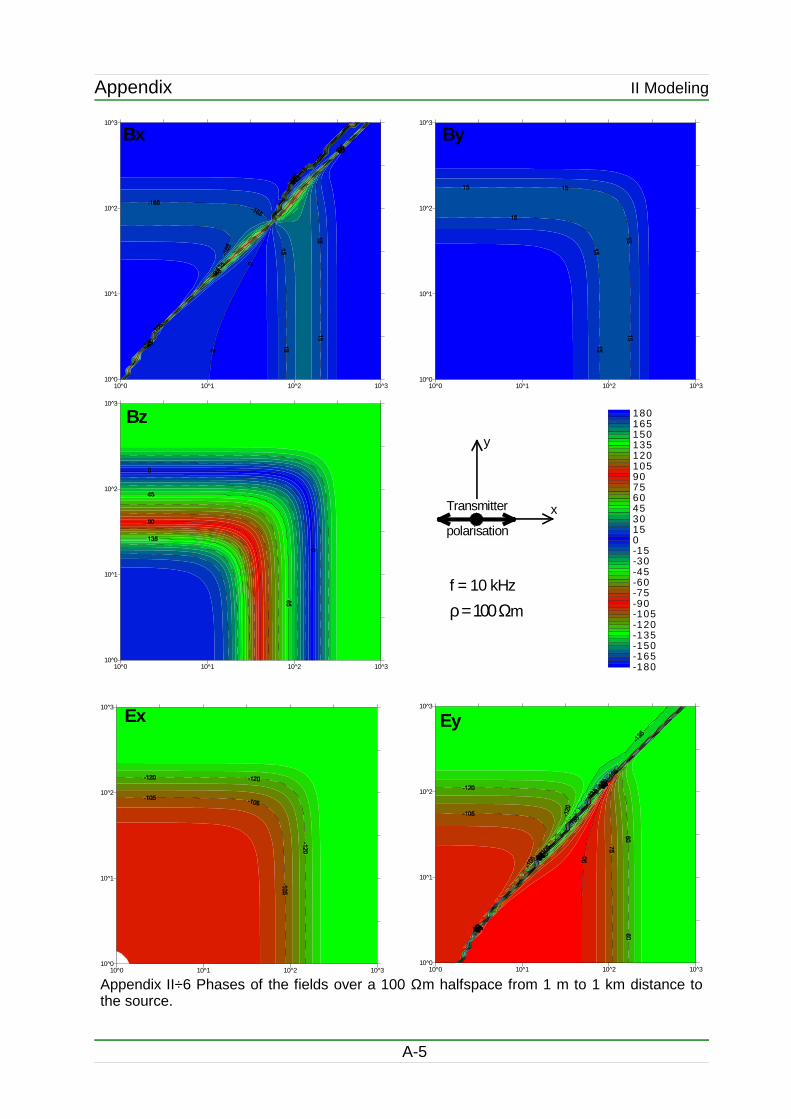
S with the power oftwo and thus it would have to be measured accurately. Using Bz itself for thesounding would prevent this problem (Bz ~ r).The phases show similar effects. Secondary fields start with 90° for Ex,y resp. 180°for Bz and meet a phase of ±45° in the far field at about 4 skin depths in thisexample. The curves can be seen in appendix II÷5.

-25-

Figure 2-3 Calculated amplitudes of the electric and magnetic fields caused by a HMD over ahomogeneous halfspace. On the abscissa the skin depth p and the induction parameter IkrI areprovided.

100 100010fT

100fT

1pT

10pT

100pT

1nT

10nT

100nT

3ppIkrI=10IkrI=1

Ex

By

Ey

BxBz

f = 10 kHz ρ = 100 Ωm

Far field approximtaion General solution

Bz,x,

y

r [m]

10-8

10-7

10-6

10-5

10-4

10-3

10-2

10-1

Ey,x

[V/m

]


2.2.2 2.2.2 2.2.2 2.2.2 Fields over a homogeneous halfspaceFields over a homogeneous halfspaceFields over a homogeneous halfspaceFields over a homogeneous halfspace

After analyzing the fields on certain profiles the spatial distribution is nowexamined. The simulations in the next chapters where done with the following parameters:

Frequency f 10 kHzHalfspace resistivity

ρ100 Ωm

Height of dipole h 1.25 mTransmitter moment

m5.000 Am²

It will be noted when different values are used. All the following contour plotsextend from 1 m to 1 km on the logarithmically scaled x- and y axis. Thetransmitter is located at the origin of the coordinate system with a polarization in xdirection.

-26-


Amplitudes

To understand the properties of thecalculated HMD apparent resistivities,it is helpful to have a look at the fieldsthemselves. Note that Bx and Ey as wellas By and Ex show correspondingspatial characteristics (Appendix II÷3).Therefore only Bx and By are shown inthe following figures. The givenexplanations mostly refer to Bx,Ey orBy,Ex jointly. Bx and Ey show a zerocrossing when they change theirorientation to get from the “north-” tothe “south-pole” of the transmitteragain (figure 2-4). By and Ex don't showthis changing of the sign but reachtheir maximum in the same region andtend to zero on the x- and y axis (figure2-5). Note that the minimum values forx or y in the regarding figure are 1 mand thus the fields don't reach a zerolevel on the lower and left margin. Thevalues of Bx or Ey depend on theazimuth from the source. The fields onthe polarization axis of the transmitterare twice as high as normal to it.Measurements in this region close tothe x axis are called collinear whereasthe area around the y axis is definedas broadside. These definitions areused to compare the resultswith the characterization ofthe HED fields in Zongeand Hughes (1988). As onecan see in this article thefields of the HED are viceversa.

-27-

Figure 2-4 Amplitudes of Bx due to a HMD at

(0,0) for x and y from 1 m to 1 km.10 0 10 1 10 2 10 3

10 0

10 1

10 2

10 3

Bx

Figure 2-5 Amplitudes of By due to an HMD at(0,0) for x and y from 1 m to 1 km.

10 0 10 1 10 2 10 310 0

10 1

10 2

10 3

By


In figure 2-6 the vertical component ofthe magnetic field is plotted. It shows aquite asymmetrical behavior, reachinga maximum in the line of the dipoleaxis and passing a zero crossing in thebroadside mode (on the y axis). Thisbehavior is in good accordance toMaxwell's equations wherejB z∪℘Ex ≠℘ y≥℘E y ≠℘ x . Ex equals

zero on the y axis and hence℘Ex ≠℘ y∪0 . In the far field Ey isindependent on x because it passesthe y axis with a constant amplitude.Hence E y ≠ xconst on the y axis. Itis an important information that tippermeasurements should be conducted inthe broadside layout though the otherfields have the weakest amplitudeshere.As one can expect the horizontal fieldsBh and Eh don't show such a behavior.They are defined as Bh∪ Bx

2≤B y2

respectively Eh∪ Ex2≤E y

2 and show

a roughly rectangular pattern. Theamplitudes of Bh can be seen in figure2-7. Eh is shown in appendix II÷4 . Mindthat the horizontal fields also showdifferent amplitudes in the collinearand broadside mode. They have thesame property as Bx and Ey in theseregions. As By and Ex have the sameamplitudes, both on thex- and y axis thecollinear/broadside relationof the horizontal fieldscomes from the propertiesof Bx and Ey only.

-28-

Figure 2-6 Amplitudes of Bz due to a HMD at(0,0) for x and y from 1 m to 1 km.

10 0 10 1 10 2 10 310 0

10 1

10 2

10 3

Bz

Figure 2-7 Amplitudes of Bh due to a HMD at

(0,0) for x and y from 1 m to 1 km.10 0 10 1 10 2 10 3

10 0

10 1

10 2

10 3

Bh


Consider a profile strike of 0° (N-S)and two transmitter polarizations.The first polarization heading to thenorth (NS polarization) and thesecond to the east (EWpolarization). The measuredhorizontal fields in NS polarization(collinear) will be roughly 2 timesas strong as the fields in EWpolarization (broadside). This ratioseems to be independent of thefrequencies but related to theresistivity. In figure 2-8 one cansee that the amplitude of the Efield changes with the frequencybut the ratio of the values at thedifferent polarizations doesn'tchange. The increase of Eh withfrequency can be explained byequation 1-5 where the relation ofthe E and B field to the frequencyand resistivity is clear. Based onconstant values of B the electricfield is coupled directly proportionalto the frequency. Around 1 kHz alittle bend introduces the near field.The vertical magnetic fielddecreases with increasingfrequency. The higher thefrequency, the better is the far fieldcondition fulfilled and Bz decreases.Note that the amplitude is quitehigh anyhow. There is nobroadside Bz plotted because thethe field passes a zero crossing onthe y axis. More descriptive nearfield conditions can be observed infigure 2-9. Here the fields arecalculated as a function of thehalfspace resistivity. In the far fieldEh and Bz increase with frequencyby a factor of . Equations 1-31to 1-33 predict this relationship. Ata halfspace resistivity of roughly100 Ωm near field effects start toexert influence. The electric fieldstend to a constant value which isthe same for both transmitter

-29-

Figure 2-8 Dependency of the electric and magneticfields on the frequency for different transmitterpolarizations.

1 10 100

10

100

Bh

[pT]

BhNS BzNS BhEW

f [kHz]

10-5

10-4

ρ=10 Ωmr = 200 m

E [V

/m]

EhNS EhEW

Figure 2-9 Dependency of the electric and magneticfields on the halfspace resistivity for differenttransmitter polarizations

0.1 1 10 100 1000 10000

1

10

100

f = 10 kHzr = 200 m

B [p

T]

BhNS BzNS BhEW

ρ [Ωm]

10-5

10-4

10-3

E [V

/m]

EhNS EhEW

Figure 2-10 Ratio of the horizontal fields in collinearand broadside measurements

0.1 1 10 100 1000 10000

1.0

1.2

1.4

1.6

1.8

2.0

r = 200 m

f = 1 kHz 4 kHz 10 kHz

BhNS/BhEW EhNS/EhEW

ρ [Ωm]


polarizations. Note that the ratio of the fields at different transmitter azimuthschanges in figure 2-10. A ratio of 1 means that Ex = Ey which implies an existenceof Zxx and/or Zyy over the simulated 1D earth. This is the only possibility for Ex = Ey

while Bx ≠=By. If Zxx∪0Z yy∪Zxy≥2Z yx while Zxx∪Z yx≥Zxy ≠2 if Z yy∪0 . This effectcan be understood when the three dimensional structure of the source isconsidered. Such as a 3D subsurface delivers values unequal zero for Zxx and Zyy

for the plane wave solution, a primary field with a finite source over ahomogeneous halfspace fills the impedance tensor with four nonzero elements.The shift of the magnetic fields when passing the far/near field border (which wasalready introduced in Chapter 2.2.2 ) can also be seen in figure 2-9. Note infigure 2-10 that the ratio of collinear to broadside field returns to the value of 2again in the near field.Mind that all these considerations were done using the quasi static approximation.In the near field regions of figure 2-9 and 2-10 at resistivities of 10 kΩm alsodisplacement currents would have to be taken into account. Then the amplitudesof the horizontal fields would not be constant.

Phases

The phases of the fields over a homogeneous halfspace show similar effects asthe amplitudes. Appendix II÷6 shows the plots for all five phases. As an examplethe phases of Ey are shown in figure 2-11. As a matter of principle two different

effects can be observed: First the change of the phasedepending on the distance from thesource marks the change from thenear into the far field. The primaryhorizontal B field phases show a trendto a level of approximately 20° overtheir normal value of 0° respectively180° in the transition zone (seeappendix II÷6). Note thatthis zone is passed at about11 skin depths (575m) onthe x and y axis concerningBy. At this distance thephase deviation goes below1° again. The correspondingranges for Bx are 8 p forbroadside and 13 p forcollinear measurements.

The secondary horizontal electric fields start with ±90° phase and meet45° respectively -135° in the far field. The distances from the sourcewhere these values are reached within a deviation of 1° are 8 p for Ex

and collinear Ey respectively 6 p for broadside Ey. Bz starts with 180°phase angle and reaches -45° ±1° at 14 p.The second effect is the 180° phase drop in the amplitude zerocrossing region of Bx and Ey.

-30-

Figure 2-11 Phases of Ey due to a HMD at (0,0)for x and y from 1 m to 1 km.

10^0 10^1 10^2 10^310^0

10^1

10^2

10^3

Ey

-180°

-135°

-90°

-45°

0°

45°

90°

135°

180°


2.2.3 2.2.3 2.2.3 2.2.3 Scalar resistivitiesScalar resistivitiesScalar resistivitiesScalar resistivities

The spatial distribution of the scalarresistivities, calculated fromorthogonal pairs of E and B fieldamplitudes (equation 1-5) are more orless self explaining. This, in Anglo -American literature called Cagniardresistivity, reproduces the features ofthe horizontal field components Bx-Ey

and By-Ex in Chapter 2.2.2. The zero crossing of Bx and Ey isreflected in figure 2-12 where theresistivities are calculated from thesetwo modeled fields. Green coloredregions in the color table mark areaswhere the synthetic HMD resistivitiesare within a range of 10 % deviation ofthe model resistivity. Again an asymmetrical behavior isobserved. In broadside mode thesynthetic scalar HMD resistivity meetsthe halfspace resistivity of the modelearlier than in the collinear fashion. Togive some quantitative facts, thedistances where the error drops below10 % is 4 skin depths in broadside and5 in collinear mode.In contrast figure 2-13 shows a quitesymmetrical behavior. Theminimum distance from thesource to get a 10 % accuratereading is 4.5 p in bothazimuths regarding thesource polarization. Theaccording ranges for thephases of the scalar HMDresistivities plotted inappendix II÷7 are 10 prespectively 6.6 p forbroadside resp. collinear Bx-Ey

and 8.7 p when using By-Ex.The relevant deviation is 1° asin Chapter . By comparisonthe ranges for an error of 2°are 7 p resp. 5 p and 6.6 p.

-31-

Figure 2-12 Scalar resistivity calculated from Bx

and Ey due to the HMD at (0,0) as in chapter2.2.2.

10^0 10^1 10^2 10^310^0

10^1

10^2

10^3

100 m +- 10%Ω

Figure 2-13 Scalar resistivity calculated from By

and Ex due to the HMD at (0,0) as in chapter2.2.2.

10^0 10^1 10^2 10^310^0

10^1

10^2

10^3

100 m +- 10%Ω

10^-3

10^-2

10^-1

10^0

10^1

10^2

10^3

10^4


2.2.4 2.2.4 2.2.4 2.2.4 RMT tensor resistivitiesRMT tensor resistivitiesRMT tensor resistivitiesRMT tensor resistivities

As discussed in Chapter 1.1.2 (Page 12) two transmitter polarizations are neededto determine the impedance tensor and therefore the resistivity tensor. Computingthese tensor values should eliminate parts of the observed source effects inchapter 2.2.3.

Dependency on position

Figure 2-14 shows the effect of thetensor treatment on the synthetic fieldsafter equations 2-9 and 1-6. Thecalculated HMD resistivity ρxy meetsthe value of the model earlier or at asmaller distance from the source asthe scalar determined HMD resistivitiesin the last chapter. In this example theranges are x10 = 3.4 p and y10 = 4.6 p inx- and y- direction. x10 or y10 stand forthe range between transmitter andreceiver where the deviation of thecalculated to the model resistivitydrops below 10 %. Note that thedefinition of the collinear andbroadside mode is no longer valid astwo transmitter polarizations contributeto the determination of the tensorvalues. In appendix II÷8 the remainingelements of the resistivity tensor areplotted. The primary diagonal elementsρxx and ρyy are close to zero as they aresupposed to. An interesting effect canbe observed comparing ρxy

and ρyx. They seem to bemirrored on the 45° axis.Even the far field distance(FFD) corresponds. Hence forρyx the ranges are x10 = 4.6 pand y10 = 3.4 p. This behaviorcan be understood when thetwo single transmitterpolarizations are observed.

For the determination of ρyx Ey has to be taken into account. For the firsttransmitter polarization (on the x axis) Ey shows the asymmetricalbehavior plotted in appendix II÷3. In the first place the amplitude incollinear mode is stronger as in the broadside and second the distancewhere the phase of Ey reaches 45° shows a higher value in the collinearmode. For the second transmitter polarization Ex in appendix II÷3 standsfor the actual Ey in this case. Due to its symmetrical distribution it does

-32-

Figure 2-14 Amplitude of the resistivity tensorelement ρxy over a 100 Ωm halfspace. Derivedfrom the electromagnetic field of a HMD at(0,0) with two dipole polarizations.

Figure 2-15 Phases of the resistivity tensorelements calculated according to fig. 2-14.

1 10 100 1000-180

-135

-90

-45

0

45

90

135

180

x = 1m f = 10kHz

ρxx ρxy ρyx ρyy

phas

e [°]

y [m]

10^-1

10^0

10^1

10^2

Ωm


not influence the behavior of ρyx. Thus the asymmetrical arrangement of Ey for thefirst transmitter polarization is reflected in the two different far field distances x10 >y10.Consider that for one specific sounding point the whole impedance tensor has tobe determined. Hence it is impossible to define a preferable measuring positionas always one of the two secondary diagonal elements of the resistivity tensor isin the “bad” mode. These modes don't differ much but with a factor of roughly 1.3which means that y10 /x10 = 1.3 for ρxy or x10 /y10 = 1.3 for ρyx.Note that all four tensor elements reach a similar magnitude in the near field. Thiscoincides with the estimation of a “full” impedance tensor for the existence ofEx=Ey when Bx≠By in chapter on page . The phases of the single resistivity tensorand tipper elements are plotted in appendix II÷9. Exemplarily the phases of allelements on a certain profile heading west (parallel to the y axis) running onemeter north of the source (x=1m) are shown in figure 2-15. All resistivities startwith a phase difference of ±90° in the near field. The secondary diagonalelements meet a phase of 45° or -135° in the far field as expected for ahomogeneous underground. The respective far field distances y1° are 8.8p for ρxy

and 6.7p for ρyx. Note the same ratio of 1.3 like just before (x10 /y10=1.3). Again thephase derived FFD y1° is greater than the one which is determined from theamplitudes (y10). Mind that 1° phase deviation is much more accurate than 10%amplitude error. Comparing the two distances quantitatively yields a factor ofquite accurate 2 for y1° / y10 resp. x1° / x10. Also the primary diagonal elements tendto phases of -45° or 135° respective 90° shifted from their corresponding primarydiagonal element regarding the magnetic component (for example ρxx and ρyx

which both are related to Bx). The amplitudes of the tipper elementsremain below 1 % as they suppose tobe over a 1D ground (see appendixII÷8 and figure 2-16). When studyingthe tipper amplitudes no near / far fielddiscrimination is possiblebut the phases of the tipperelements show a similartrend as the tensorresistivities. Tipper phasesstart with 180° and meet-45° in the far field. Incontrast to the behavior ofthe far field distances of thesingle resistivity tensorelements the spatial tipperphase distribution is exactlysymmetrical and equal forTx and Ty. The x1° resp. y1°

distance equals 5.7 skindepths. In this case x,y1° is

more a mathematical value than an usable field factor. As the tipper

-33-

Figure 2-16 Amplitude of the tipper element Tx

over a homogeneous halfspace. Derived fromthe electromagnetic field of a HMD at (0,0) withtwo dipole polarizations. The yellow area marksvalues above 1 %.

10^0 10^1 10^2 10^310^0

10^1

10^2

10^3

Tx

10^-4 %

10^-3 %

10^-2 %

10^-1 %

10^0 %


phase is not descriptive it won't be discussed in the following. The certain plotswill be provided in the respective appendix pages. Not the phase, but theamplitude plays the important role for CS tipper measurements. Over a layeredhalfspace the source induced tipper must tend to zero to permit anymeasurements. As one can see in figure 2-16 this criteria is fulfilled in almost thehole area. The tipper amplitude stays below 1% outside of a 2 m distance (yellow)which is much too narrow anyhow. Remember that in the scalar mode tipper measurements are not possible as thevertical magnetic field doesn't die off fast enough with distance. Measuring withtwo transmitter polarizations allows to conduct tipper measurements also undernear field conditions for impedance measurements.

-34-


Dependency on frequency and resistivity

As the spatial description of themodeled HMD resistivities is just asnapshot for one single frequencyand halfspace resistivity, thedependency on these variables isnow discussed. For bettertransparency one element of theresistivity tensor ρxy is picked for alloncoming investigations. It is ofspecial interest if and how the near /far field border changes withfrequency and resistivity. Figure 2-17delivers both answers. All the curvesrepresent simulations on one certainsounding point with the coordinates(x = 500, y = 10 m). Simulations weredone for 12 resistivities from 10 Ωmto 1 kΩm logarithmically spaced in afrequency range from 100 Hz to 100kHz. The dependency on thefrequency can be observed best withthe curve for one halfspaceresistivity, for example 100 Ωm. Atfrequencies above 3 kHz thecalculated resistivity meets themodel value properly thus thesounding point is in the far field.Below this frequency the transitionzone to the near field starts. Atroughly 200 Hz the curve meets the

near field asymptote where the calculated HMD resistivities decrease linear withthe frequency. If the curves of several resistivities are now compared under thispoint of view, one can see that the far field / transition zone border is shifted tohigher frequencies when the halfspace resistivity increases. As we are stillregarding a homogeneous halfspace, the phases start at -90° and meet -135° inthe far field independent on frequency or resistivity (figure 2-18). In contrast, thedistance where it reaches this value depends nevertheless on the resistivity. Theeffects are comparable to the amplitude behavior. For example the frequency inwhich the 100 Ωm phase meets 135° is 8 kHz.

-35-

Figure 2-18 Phases of ρxy in figure 2-17.

0.1 1 10 100

-135°

-120°

-105°

-90°

ρa= 10 kΩm

x = 500 m y = 10 m

ρa= 10 Ωm

ρa= 1 kΩm ρa= 100 Ωm

Φ(ρ

xy) [

°]

f [kHz]

Figure 2-17 Calculated resistivity tensor elementρxy at (500,10) for different halfspace resistivities asa function of frequency. Derived from theelectromagnetic field of a HMD at (0,0) with twodipole polarizations.

0.1 1 10 100

10

100

1k

10k ρa= 10 kΩm

x = 500 m y = 10 m

ρa= 10 Ωm

ρa= 1 kΩm

ρa= 100 Ωm IρxyI [

Ωm]

f [kHz]

Chapter: Modeling 2.3 Two layer case

2.3 Two layer case

After studying the features of calculated CSRMT measurements over ahomogeneous halfspace a few examples for resistivity changes with depth arediscussed in the following subchapters. As it is impossible to compute everygeologically possible structure, only basic effects are considered. In order to compare the results of the next simulations with the homogeneoushalfspace responses, the MT apparent resistivity of all models is 100 Ωm for10 kHz.

2.3.1 2.3.1 2.3.1 2.3.1 Conductive overburdenConductive overburdenConductive overburdenConductive overburden

To study the spatial distribution of thecalculated HMD apparent resistivities,the resistivity tensor was computed asin Chapter 2.2.4 with the followingmodel: Over a ρ1 = 1 kΩm halfspacelies a conductive layer with ρ2 = 10 Ωmresistivity and a thickness of t = 2.73 m.The phase of the MT apparentresistivity of this model is 14°. Theresults are plotted in appendix II÷10and II÷11 respectively figure 2-19 and2-20. In figure 2-19 an increase of thefar field distance can be seen. Theupdated ranges are x10 = 6.6 p andy10 = 9 p if the little stripe where theHMD apparent resistivity reaches89 Ωm on just one sounding point in y-direction is neglected. The ratioy10 / x10 = 1.36 in this example. Theexplanation for these increased farfield distances must be foundin a current channeling effectof the conductive layer. Alsothe phases meet their far fieldvalue of 14° or -166° atgreater distances. Thecharacteristic values arex1° = 12 p and y1° = 14 p. Infigure 2-20 exemplary phasecurves are plotted where adrastic slope of the primarydiagonal elements phase canbe seen.

-36-

Figure 2-19 Amplitude of the resistivity tensorelement ρxy over a 2 layer halfspace withconductive overburden and MT apparentresistivity of 100 Ωm for 10 kHz. Derived fromthe electromagnetic field of a HMD at (0,0) withtwo dipole polarizations.

10^0 10^1 10^2 10^310^0

10^1

10^2

10^3

xyρ 100 m 10%Ω

Figure 2-20 Phases of the resistivity tensorelements over a 2 layer structure withincreasing resistivity. Derived according to fig.2-19.

1 10 100 1000-180

-135

-90

-45

0

45

90

135

180

x = 1m f = 10kHz

ρxx ρxy ρyx ρyy

phas

e [°]

y [m]

10^-1

10^0

10^1

10^2

Ωm


2.3.2 2.3.2 2.3.2 2.3.2 Resistive overburdenResistive overburdenResistive overburdenResistive overburden

To give an example for a model inwhich the resistivity decreases withdepth, an overburden with 1 kΩm anda thickness of 33.3 m over a 1 Ωmhalfspace is introduced. Again thecumulative MT apparent resistivity for10 kHz is 100 Ωm and the phase 84° or-96°. The results of the simulations areshown in appendix II÷12 and II÷13 aswell as in figure2-21 and 2-22. In contrast to theconductive overburden here the farfield distance decreases explicitly.x10 = p if the single value of 112 Ωm atx = 95 m is neglected. Note that thisrange of 50 m makes no sense for thefield as the geometry of the transmittercoil limits the minimum separation oftransmitter and receiver. Therespective relationships are given inchapter 1.2.2 on page 15. Outsides ofthe deviation band between y = 100and 180 m which reaches an error of16 %, y10 equals 3.6 p. If this zone isalso neglected, y10 would be 1.3 p. Withthis value y10 / x10 would be 1.3 again.Regarding the phases, it is worthmentioning that the drop of the curvesis not as rapid for the primary diagonalelements as over the conductiveoverburden or even over thehalfspace. This leads to theconclusion that the morepositive the resistivitycontrast is, the sharper anddeeper the decline of the ρxx

and ρyy phases has to be.The respective FFDs arex1° = 1.3 p and y1° = 1.9 p whichyields a ratio y1° / x1° of 1.46.

-37-

Figure 2-21 Amplitude of the resistivity tensorelement ρxy over a 2 layer halfspace withresistive overburden and MT apparentresistivity of 100 Ωm for 10 kHz. Derived fromthe electromagnetic field of a HMD at (0,0) withtwo dipole polarizations.

10^0 10^1 10^2 10^310^0

10^1

10^2

10^3

xyρ100 m 10%Ω

Figure 2-22 Phases of the resistivity tensorelements over a 2 layer structure withdecreasing resistivity. Calculated as in fig. 2-21.

1 10 100 1000-180

-135

-90

-45

0

45

90

135

180

x = 1m f = 10kHz

ρxx ρxy ρyx ρyy

phas

e [°]

y [m]

10^-1

10^0

10^1

10^2

Ωm


2.3.3 2.3.3 2.3.3 2.3.3 Dependency on resistivity contrastDependency on resistivity contrastDependency on resistivity contrastDependency on resistivity contrast

After discussing two single cases of a 2 layered structure now the changes of thecalculated HMD apparent resistivity tensor regarding the resistivity contrast K ofthe several layers is being studied.Simulations were done with 13 different values for K∪log 1≠ 2 from -5 to 5.The particular thickness t of the layer with ρ1 which overlays a halfspace with ρ2 ischosen to meet an apparent MT apparent resistivity of 100 Ωm for 10 kHz. A tablewith the used resistivities and thicknesses is given in appendix II÷14.

In order to achieve transparency onlythe tensor element ρxy is being studiedalong one profile in x- direction. As it isshown in the last chapters, thisconfiguration yields a far field distancewhich is less than concerning ρyx onthe x axis or ρxy on the y axis. But alsothe ratio of these two certain distancesis quite stable around 1.3. This makesit possible to transfer the one valueinto the other. The range x10 in the ρxy

configuration can be understood asthe minimum separation where one ofthe HMD apparent resistivity tensorelements meets its far field value.

-38-

Figure 2-23 Amplitudes of ρxy along a profile in x- direction at y = 5 m for differentK = log(ρ1 /ρ2) with f = 10 kHz. Derived from the electromagnetic field of a HMD at(0,0) with two dipole polarizations.

10 100 10000

25

50

75

100

125

150

K (+) (-)5 4 3 2 1 0.3 0

ρ xy [Ω

m]

x [m]

Figure 2-24 Phases of ρxy in figure 2-23.

10 100 1000

-180

-165

-150

-135

-120

-105

-90

0

K=

-3

-1

1

35

ρ1 > ρ2

ρ1 < ρ2

x [m]

Phas

e(ρ xy

) [°]


Increasing the distance of 30 % sets the sounding point into the “real” far field.The way the FFD changes with K can be seen in figure 2-23. The results of thelast chapters imply an increase of x10 with K which is illustrated now. A conductiveoverburden (K < 0) results in a more intensive change of ρxy in comparison tomodels with K > 0. Note that for -4 < K < -0.3 the single curves of the resistivitychange much more than for K = -5 and -4. This seems to be some kind ofsaturation effect. A resistive overburden doesn't change the calculated HMDapparent resistivity values in such a way. There are significant differencesbetween the curves for K = 0, 0.3 and 1, but for K = 2 to 5 the changes are quitesmall. As in other electromagnetic methods, good conductors influence thesystem more than poor conductors. In figure 2-24 (where the respective phasesare plotted) one can see that there are some changes in the phase for K > 2.

Note that the FFD decreases continuously with increasing K. To evaluate theconnection of x10 and K, different resistivity contrasts were tested with the FFDestimation program introduced in chapter 2.1.3 on page 23. Up to this pointvalues for x10, y10, or x1°, y1° were picked manually. Figure 2-25 shows the results ofthe calculations. Mind the offset of the curves for x5 and x10 respectively x1° and x2°

to each other as the FFD decreases with increased allowable deviation. On theright hand side of the plot resistive overburdens are represented. The FFD staysat or just below the homogeneous halfspace value. Only when the phase criteriais taken into account, the FFD drops continuously with increasing K. On the lefthand side, in which conductive overburdens appear, the FFD increases rapidlywith an increasing value of negative K. Regarding the phase, the minimum farfield range reaches values above 1 km early. Even when an amplitude error of10° is accurate enough, the FFD gets almost 3 times as high as over thehomogeneous halfspace. In appendix II÷15 and II÷16 some more curves for otherallowable deviations are given.The trend that the FFD increases drastically when simulations with a conductiveoverburden are done, generally points out a sort of current channeling in the lowresistivity layer. This effect may cause serious problems for CSRMT field work.

-39-

Figure 2-25 Far field distances for 5 %, 10 %, 1° and 2°deviation depending on K = log(ρ1 /ρ2).

-4 -2 0 2 40

200

400

600

800

ρ1>ρ2ρ1<ρ2

x10 x2° x5 x1°

Far f

ield

dist

ance

[m]

K=log(ρ1/ρ2)

Chapter: Modeling 2.4 Far field distance estimation

2.4 Far field distance estimation

After studying the effects of the certain resistivity contrasts on the FFD, a fieldformula to estimate the minimum range between transmitter and receiver isdeveloped now.Therefore several calculations of the FFD x1 concerning ρxy for differentfrequencies from 10 Hz to 1 MHz dependent on the subsurface resistivity weredone. For the frequencies 1 to 100 kHz also the 10 % deviation FFD x10 wascomputed. Appendix II÷17 shows the certain curves. Note that for highfrequencies and resistivities the slope changes as the quasi static approximationis no longer fulfilled. This plot can be used like similar figures for the skin depth tofind out the actual far field distance in the field when the resistivity of thesubsurface is roughly known which is the case in most geophysical surveys.Knowing the frequencies of the used system one can easily determine theminimum range between transmitter and receiver.

The second interesting magnitude for field work is the amplitude of thefields which have to be measured at the sounding point. It is clear thatthe maximum distance is limited by this field strength and theresolvability of the receiver. To crosscheck these two values thehorizontal magnetic field was also computed for certain resistivitiesand distances. The magnetic field was chosen as a limiting factor asthe measured electric field is increasable by a larger electrode spacingif the signal gets to low. Calculations for 1, 10 and 100 kHz are plottedin appendix II÷18. Figure 2-26 shows a combined plot of the twointeresting magnitudes. Exemplary x10 and x1 for the three frequenciesare shown (x10 as the thicker line) with their relating Bh values in thebackground. This plot makes it easy to have a quick look on theestimated minimum transmitter receiver separation and to see if theused instrument is able to measure the field strength at this distance.The magnetic field in figure 2-26 is calculated with a fixed transmittermoment of 5000 Am². Working with the transmitter used for this thesisthe current in the transmitter coil decreases with increasing

-40-

Figure 2-26 FFD and Bh for 1, 10 and 100 kHz depending on the halfspace resistivity (x10 as thethick; x1 as the thin line).

nT

pT

nT nT

pT

1 0 - 1 1 0 0 1 0 1 1 0 2 1 0 3 1 01 0

1 0 0

1 0 0 0

101

ρ a [Ω m ]

m = 5.000 Am²

x , x

[m

]1

10

10^-15 T

10^-12 T

10^-9 T

10^-6 T


frequencies and thus the transmitter moment goes down. In appendix II÷19 a plotlike figure 2-26 is provided in which different moments for the single frequenciesare taken into account. Except at 100 kHz no significant change is observed.The curves for x10 respectively x1 show a linear behavior in the double logarithmicscale. Hence a linear regression with these data was done. For the regressionfollowing relationship was assumed:

log x1∪A f ≤B f log a x1∪10A f a

B f (2-10)

The results with x1 in meter and ρa in Ωm are:

SD stands for the standard deviation of the values from the regression result.Plotting the factor A and B over the logarithm of the frequency also yields a lineardependence of the form

A f ∪1.896≥0.4867 log f ∋ 1.9≥0.5 log f

B f ∪0.4924≥0.003 log f ∋ 0.5

x1∪101.9≥0.5 log f a ∪ 101.9 a

f

(2-11)

which results in a field formula for the 1 % FFD of

x1∋79a

fwith x m , τm , f kHz

.(2-12)

The same proceeding on x10 yields

-41-

A (f) B (f) SD1 1.896 0.493 0.0033 1.652 0.491 0.00510 1.412 0.489 0.00732 1.167 0.488 0.006100 0.922 0.487 0.008

f [kHz]

A (f) B (f) SD1 1.75 0.502 0.0033 1.499 0.503 0.00510 1.237 0.507 0.01432 0.97 0.513 0.021100 0.744 0.503 0.003

f [kHz]


as well as

A f ∪1.748≥0.5082 log f ∋ 1.75≥0.5 log f B f ∪0.503≥0.003 log f ∋ 0.5

x10∪101.75≥0.5 log f a ∪ 101.75 a

f

(2-13)

which delivers a 10 % FFD of

x10∋56a

fwith x m , τm , f kHz . (2-14)

Note that these two field formulas (2-12) and (2-14) have a similar form as theskin depth formula

p∪ 20ᵀ

. (2-15)

Taking into account that ∪2000 f kHz , 0∪410≥7 and ᵀ∪1≠a τm

yields

p∋16a

f. (2-16)

Both p and x1 or x10 depend on a ≠ f just with different scaling factors. Buildingthe ratios of these parameters delivers the following dependencies:

x10∋3.5p x10∪3.520p

x1∋5p x1∪4.949p(2-17)

Remember these are the minimum ranges which have to be increased by 30 % toget into the definitive far field.

-42-

Chapter: Modeling 2.5 Summary of the modeling results

2.5 Summary of the modeling results

For the sake of clarity the most important properties of the electromagnetic field ofa horizontal magnetic dipole as well as the resulting calculated HMD apparentresistivities are given in the following list.

The amplitudes of the fields and HMD apparent resistivities meet the far fieldcondition at smaller distances from the source than the respective phases.

In the collinear mode the magnetic field contains a vertical component with asignificant magnitude which has to be taken into account if scalar tippermeasurements are conducted. As the vertical field tends to zero in thebroadside mode, the determination of the tipper vector eliminates this effectdue to the incorporation of two transmitter polarizations.

The spatial distribution of the horizontal electric and magnetic field shows adifference of the specific amplitudes in collinear and broadside mode. Theamplitude in the line of the transmitter polarization is twice as high as in thebroadside mode.

The far field distances of tensor resistivity values are smaller than the FFDs ofscalar derived resistivities. Regarding the resistivity tensor element ρxy the FFDin y- direction is thirty percent greater than in x- direction. This effect isvice versa for ρyx.

The presence of a conductive overburden affects the far field distance strongly.A resistivity contrast of just two magnitudes at least doubles the FFD. Minimumranges between transmitter and receiver beyond one kilometer are reachedquickly.

A linear dependency between far field distance and skin depth was found. Thedeviation between the amplitudes of the HMD- and the MT apparent resistivityreaches one percent at five skin depths respectively ten percent at 3.5 skindepths.

-43-

3 Instrument

-44-

Chapter: Instrument 3.1 Receiver

3.1 Receiver

The RMT receiver used in this work was developed in the finished researchproject with the title “Klärung des methodischen Potentials einer vielkanaligengeophysikalischen RMS-Apparatur mit HTSL-SQUID”. The aim of this project wasto evaluate the potentials of SQUID magnetometers for geophysical EM methods.A detailed presentation of the system can be found in Radic and Burkhardt(2000).

3.1.1 3.1.1 3.1.1 3.1.1 Technical specificationTechnical specificationTechnical specificationTechnical specification

A brief description of the main parameters of the receiver is given in the followingtable:

Further highlights are 8 digital down converters (DDCs) which extract singlefrequencies from the time series and a digital signal generator which provides asine voltage for calibration purposes.

The system is powered by internal chargeable batteries which last forapproximate one field day.

-45-

Channels 5Sampling frequency 2.5 Mhz

A/D resolution 16 bitBandwidth 400 Hz – 1.25 Mhz

Figure 3-1 Picture of the RMT receiver with connectedcontrol laptop.


The five channels are used to measure 3 magnetic and 2 electric fieldssimultaneously. Magnetic signals are picked up with a triple of orthogonal

shielded coils. Figure 3-2 shows the three copper pipe loops which cover the coilwindings from electric fields. The specifications of the B sensors are given in thenext table:

Both magnetic and electric sensors are connected to the receiver by a 10 m BNCcable. The preamplifier for the electric fieldsconverts four poles and one common ground.Hence it is possible to work in X- and L- layout.Both electric and magnetic preamplifiers havean individual power supply which has to becharged after the field day. The technical data isgiven in the following table:

-46-

Figure 3-2 Picture of the magnetic sensors.

Channels 3Area 0.5 x 0.5 m²

5WindingsBandwidth 1 kHz – 1.25 Mhz

System noise 1 fT/√Hz

Figure 3-3 Picture of electricpreamplifier.

Channels 2Dipole 1 – 16 m

Bandwidth DC – 1.25 MhzSystem noise <10 nV/√Hz


3.1.2 3.1.2 3.1.2 3.1.2 The control panelThe control panelThe control panelThe control panel

After the preprocessing in the receiver the measured data are transferred to thecontrol laptop where the saving and final field processing is done. The control ofthe measurement and calibration is also conducted by this computer. For thispurpose a LabVIEWTM program had been developed during the mentioned

finished SQUIDproject. In figure 3-4 atypical screen duringa measurement isshown. In the centralpart the time series ofthe specific channelscan be observed tocheck data qualityand saturation of theA/D converters. Thedisplayed time seriesare alreadydownconverted whichmeans that theycontain just a narrowfrequency bandwidth.On the upper left side

the actual measuring frequency can be chosen and some configurations can bemade. The lower left side contains buttons for certain subroutines like calibration,configuration or scanning for transmitter frequencies. On the right hand side it ispossible to set the frequencies for the measurement. This was the status of the controlling software which had to be adapted forCSRMT requirements. The following main changes were necessary:

Adapting an existing transmitter control program to find the resonancefrequencies of the system

Introducing the communication with the transmitter via serial bus or radiomodem into the measuring program

Adding a CSRMT mode to the front panel of the measuring program

Reworking the sounding and processing routine for the altered requirementsdue to the source mode

A few comments on the single tasks are given in the following.

-47-

Figure 3-4 Screenshot of the front panel of the RMT control program.


Adapting the source control routine

As it will be shown in chapter 3.2.1, the transmitter contains a serial resonancecircuit. To find the resonance frequencies for the given capacitor combinations,the stimulation frequency has to be varied in small steps.First the program calculates the necessary capacity for a chosen frequency usingan estimated value for the inductivity of the transmitter coil. A combination of thebuilt in capacitors, which meets the desired capacity best, is activated. Thesystem is stimulated with the chosen frequency which is changed to higher orlower values depending on the observed current in the coil. When this currentreaches a maximum the resonance frequency is found.Measurements of this kindcan be found in chapter 4.2.1.

Communication

The transmitter is connected to the field computer via the serial port. Forcommunication a DOS program was provided. As the Metronix company kindly provided a radio modem, it was possible tocontrol both receiver and transmitter with just one field laptop. Therefore thecommunication between laptop and transmitter respectively laptop and receiverhad to be separated. This caused no technical problem as the receiver uses theparallel port of the notebook. For the software it was necessary to avoid asimultaneous use of both ports.The DOS source control executable asks for a hexadecimal code containing theinformation which relays in the transmitter have to be switched. The DOSprogram converts this code into certain signals on the serial port. Due to this fact,the CSRMT control program doesn't run under Windows NT. Depending on thegiven tasks, the LabVIEWTM control panel creates a batch file containing allneeded callings of the DOS executable file.

The new front panel

The so called front panel of the CSRMT control program is the main level fromwhere all functions are started or configured. Here it is possible to check thesignals at the used frequencies as time series or spectra before starting asounding. In this View-mode the system is acquiring and plotting datacontinuously. If the frequency is changed, the digital downconverters of thereceiver provide the laptop with data containing this frequency information. Whenusing the active mode not only the receiver but also the transmitter changes theactive frequency. A frequency change of the transmitter contains the followingsteps:

Turning the stimulation amplitude down to zero Switching off the amplifier Setting the relays for the capacitors Setting the relay for the transmitter polarization Switching on the amplifier Setting the stimulating amplitude and frequency to the adjusted value

-48-


Once tuned in to one frequency it is possible to change the amplitude of thestimulating signal in the transmitter to find the best compromise between properreceived signal and low amplitude in the transmitter to save battery power andprevent the amplifier of getting too hot. When the optimum configuration is found,the amplitude can be taken into account for the following sounding. It is possibleto work with different stimulation amplitudes for each individual frequency. Note that when the single channels are checked for maximum saturation at theselected frequencies, the displayed time series or spectra contain only a narrowfrequency bandwidth. To see the data without any preprocessing, one must checkthe saturation with the scan routine where unprocessed time series aretransferred to the laptop and are displayed without any manipulation. This is away to see the raw field data which is also used for some measurements in

chapter 4.2.3.The finally designed CSRMT control panel shown in figure 3-5 contains the toolsto work with the transmitter from the laptop which is connected to the receiver aswell. On the upper right corner the various selectable frequencies for bothtransmitter polarizations are displayed. They were determined as describedbefore. The LED like looking buttons between the specific almost equalfrequencies for the different polarizations allow to choose if they should be usedfor the sounding or not. Below this frequency block a switch to set the currentlyused transmitter polarization is provided. The next control with the title “Amp”allows to set the actual stimulating amplitude in the transmitter in mV. The list inthe lower right corner contains the amplitudes “Amps [mV]” which will be used forthe single frequencies in the sounding. The button next to the letters “F4” on the

-49-

Figure 3-5 Screenshot of the CSRMT control program.


left side of the screen switches from the active to the passive measuring mode.After clicking the button or pressing the F4 key the screen will look like figure 3-4again.

The new sounding routine

The use of digital down converters (DDCs) enhances the speed of passive RMTmeasurements. The basic principle is measuring one time series, preprocessingthe data with 8 DDCs simultaneously and transferring 8 decimated binary datasets to the laptop. As explained before, a DDC extracts a narrow band around agiven frequency from the raw data. The result is again a time series with less datapoints than before. As measuring time decreases as the amount of data whichhas to be transferred decreases with the decimation. As one active measurement contains just one frequency, this procedure had to bechanged. Conducting CSRMT measurements, the polarization of the transmitteror the frequency of the DDC and the transmitter are alternately changed.Measuring time increases as several registrations and decimations have to bedone. As the switching of the transmitter takes a certain time the measuringroutine must wait for the transmitter before the next registration is started. When all the data is collected the processing is also different from the passivetype. As one single measurement contains all frequencies and polarizations in thepassive mode, the impedance tensor can be calculated directly from thisinformation. Dealing with the controlled source yields a number of data sets whichhave to be combined to determine the tensor information. Therefore the data hasto be sorted and joined in a way that it fits for the passive tensor calculationroutine.Optionally the results of the CSRMT measurement can be combined with thepassive data to one continuos sounding.

-50-

Chapter: Instrument 3.2 Transmitter

3.2 Transmitter

Figure 3-6 shows a principal sketch of the transmitter. The basic features are:

Two vertical standingloops connected inseries to

a battery of capacitorsforming a serialresonance circuit.

A signal generator tostimulate the circuitand

an amplifier to achievehigh currents.

The provided system (except the signal generator) was a prototype contributed tothe SQUID project by the Metronix company, but was never used in this project.

3.2.1 3.2.1 3.2.1 3.2.1 Technical descriptionTechnical descriptionTechnical descriptionTechnical description

Before describing the alterations to the system the single components are brieflyintroduced in the following.

The signal generator was built by “Linau industry electronics” and works in a frequency range from 0 to250 kHz. Its output voltage reaches up to 960 mV in 13 linear spaced steps. As itjust acts as stimulating input for the amplifier, the maximum current is irrelevant.The generator is controlled by the serial port of the notebook directly. Thegenerator is connected to the relays of the capacitors via a zero modem cable.

The amplifier

is a 250 watt (at 4 Ω) mono car audio amplifier. It is a Rockford Fosgate “Punch250.1 power” with a specified bandwidth of 10 Hz to 200 kHz. The power rating ofthe manufacturer yields a frequency range from 20 Hz to just 20 kHz with lessthan 0.1 % total harmonic distortion. The casing consists of an aluminum castheatsink.

The capacitors battery

consists of fourteen capacitors from 10 µF down to 470 pF. They are spaced 10,4.7, 2.2, 1, 0.47, ... to reach specific values most accurately. Relays allow toconnect them in parallel. The maximum capacity is therefore ≈18.78 µF.

-51-

Figure 3-6 Sketch of the transmitter parts.

Amp

Signal generator Amplifier

Capacitor battery

Polarization switch

Loops

Batteries

Radio modem


The loops

are made of high voltage cables with 5 wires which are connected in a way thatthey represent loops of 5 turns. The cables have a length of 25 m to form a10 x 2.5 m² rectangle in the field. The loops are mounted on overall 5 rods which

are tightened to theground with straps tokeep them in a verticalposition. The layout ofthe coils is equivalent toan L, where one isoriented to the west andthe other orthogonal to it.A typical field layout canbe seen in figure 3-7.Due to the differentresonance frequencies itis important that for eachpolarization the sameloop cable is being usedfor every field day.

3.2.2 3.2.2 3.2.2 3.2.2 ImprovementsImprovementsImprovementsImprovements

At the beginning of thiswork the transmitter wassupplied with an externalsignal generator. Thecontrol laptop wasconnected to the signalgenerator and from thereto the relays for theamplifier and capacitors.Because of intenseheating the case had tobe opened most of thetime to cool the amplifier.Figure 3-8 gives animpression of how thislooked like in the field. To

the left of the blue transmitter casing two of the rods to mount the loops can beseen. Next to the two batteries stands the 30 A battery charger connected to apower generator approximately 50 m away.Regarding the transmitter two main problems had to be solved:

Excessive power consumption and “system melting” heat production.

-52-

Figure 3-7 Built up transmitter loops in the field. The loop cablesare highlighted by orange lines.

Figure 3-8 The start up configuration of the RMT source.

Signal generator

Capacitor batteryAmplifier

Control laptop


Power supply

The problem with the immense power consumption of roughly 55 A DC whiletransmitting was solved with the help of a 2 kW power generator in the field.During the measurements the two 143 Ah batteries for the transmitter werecharged continuously by a 30 A 12 V battery charger. This prevented thetransmitter from going down just after approximately 5 hours. With the permanentcharging it was also possible to measure on several days, as it would have beenimpossible to charge two 143 Ah batteries over night. After this change a new problem arose. The signal generator stopped to react toprogram calls when the power generator was running. It turned out that the signalgenerator was sensitive to supply voltages beyond specifications. To prevent thisproblem a voltage regulator was installed.

Heat production

Besides the power supply the more serious problem seemed to be theoverheating of the amplifier and the capacitors at high currents. It happened quite soon that one of the capacitors melted under field conditions.The problem of the system layout is, that at certain desired capacities just a fewor even only one or two capacitors are switched on. Then the whole current of thesystem (up to 50 A) runs through these two or three capacitors and heats themup. Even when more capacitors are being used, more than half of the currentflows through one capacitor. In figure 3-9 the distribution of the current throughthe single capacitors is shown. Capacitor #1 stands for the one with 10 µF. Thecapacity decreases with increasing number (for example cap. 10 / 10 nF). Alisting of all the capacitors and percentile currents is given in appendix III÷1. Notethat the 0.22 µF capacitor (cap. #6 in figure 3-9) melted when working with 8 kHz.This melted capacitor was replaced by a stronger type of the same capacity. For

the used frequencies of 1, 2, 4,8, 16, 32 and 40 kHz the rest ofthe capacitors were quite stable.Tests with frequencies between40 and 200 kHz showed rapidtemperature increases at theused capacitors and besidesthat a breakdown of theamplifier which will bediscussed later.Generally the performance ofthe system is limited by theamplifier. Although it ought tobe able to handle frequenciesup to 200 kHz it fails alreadyaround 30 kHz. The amplifierseems to be not fast enough toprovide the output with a highfrequency sine current. This canbe seen using an oscilloscope.

-53-

Figure 3-9 Distribution of the system current among thesingle capacitors of the transmitter for differentfrequencies.

1 2 3 4 5 6 7 8 9 10 11 12 13 14

1 kHz

4 kHz

16 kHz

64 kHz0

10

20

30

40

50

60

70

80

90

curr

ent [

%]

capacitor

Freq

uenc

y


Especially at these high frequencies the casing of the amplifier gets extremelyhot. To transport the heat from the amplifier out of the transmitter housing aventilation system with a powerful 12 V fan was installed. To avoid overheatingdamages of the amplifier a temperature controlled security switch off had beenintegrated. Nevertheless the amp broke down two times. The first time it wasrepaired by the manufacturer without charge who gave the information that

exactly this security switch broke and didn't switch on again. The second time theheat load had been more damaging and the power transistors were broken andblack from smoke or flames. This was the moment when we stopped investingany more time and energy in this system as it didn't meet the requirements.Figure 3-10 shows the transmitter after all alterations were finished. The signalgenerator is mounted internally and a radio modem is connected instead of thelaptop. The two circular grids on the left side of the top of the casing are the air in-and outlet for the cooling fan. The batteries are connected to a charger whenprofiling work is done.

-54-

Figure 3-10 The reworked transmitter system with radiomodem.

4 Measurements

-55-

Chapter: Measurements 4.1 Laboratory

4.1 Laboratory

4.1.1 4.1.1 4.1.1 4.1.1 Transmitter outputTransmitter outputTransmitter outputTransmitter output

Before the transmitter was taken out to the field, its characteristics wereevaluated during measurements in the laboratory. The amplifier was stimulated with a manually adjustable signal generator. One ofthe loops was laid out on the floor to simulate the interplay of capacity andinductor. Varying the stimulation frequency of the signal generator the resonancefrequencies for the specific capacities were found rapidly. The lowest achievedfrequency was 1.33 kHz when all capacitors were switched on (/.18.8 µF) andthe maximum was reached at 165 kHz with no activated capacity. For thisfrequency range two different investigations were carried out. First the stimulating voltage was increased until the amplifier reached itsmaximum deliverable current at the certain frequency or the temperature of anyactive capacitor reached a dangerous level. At frequencies above 30 kHz theheat production of the capacitors limited the performance of the system. Therapid temperature increase allowed maximum transmitting durations of only oneminute. Besides the capacitor temperature the harmonic distortion of the amplifierrestricted the performance. In detail at 35 and 66 kHz the heat productionrespectively at 142 and 165 kHz the harmonic distortion limited the maximum

reachable current in the loop. Thedashed line with the circles in figure4-1 shows the reached currents forthe specific frequencies. In the fieldit turned out that at lowerfrequencies the capacitors were notthe problem, but the amplifier wenttoo hot when the transmitter wasactive for several minutes.The second observed value was thevoltage which was necessary toproduce a current of 10 A in theloop. These voltages are plotted asa dotted line with open boxes infigure 4-1. For frequencies over

35 kHz no voltages are displayed as the maximum achievable currents lay below10 Amperes. Note that the maximum voltage of the system signal generator is980 mV.As a result of these tests the maximum transmitter frequency for the field was setto 40 kHz to prevent the system from heat damages. Besides the temperatureproblem the current amplitudes are very small at higher frequencies anyway. Forthe two “high” frequencies 32 and 40 kHz a security routine was implied into thecontrol program which switches the signal generator off after one minutetransmitting time.

-56-

Figure 4-1 Maximum achievable current of theamplifier and needed voltage for 10 A systemcurrent.

1 10 1000

10

20

30

40

Max

imum

cur

rent

[A]

Frequency [kHz]0

250

500

750

1000

Stim

ulat

ing v

oltag

e fo

r I=1

0A [m

V]


4.1.2 4.1.2 4.1.2 4.1.2 CalibrationCalibrationCalibrationCalibration

The CSRMT control program is provided with the possibility to calibrate thesystem. During this calibration the effects of the sensors, preamplifier, cables andthe receiver systems like A/D converter etc. are eliminated. As only ratios ofcertain field pairs like Ex / By or Bz / Bx are important to determine the impedanceand tipper, only these ratios are calibrated.

The technical layout is described inthe following. The receiver coil tripleis brought into a position where allmagnetic dipoles are orienteddownwards with the sameinclination. Around the antennas ahorizontal single loop is placed withthe coil triple in the center. Thecoupling between the horizontalcalibration coil and the singlereceiving loops is equal, which yieldsa ratio of Bz / Bx = Bz / By = 1. Tomeasure the electric fields as well, aresistor is integrated in thecalibration loop wire on which thevoltage for the E field is picked up.The channels Ex and Ey areconnected to the same resistor. Thisyields values of Ex,y / By,x which are afunction of the resistance and themutual inductance of the calibrationloop and the receiver coils. When acalibration measurement isconducted, the sixth channel of thereceiver which supplies thecalibration signal is connected to thecalibration coil. It delivers sinesignals with the desired calibrationfrequencies. During the calibrationloop is transmitting the ratios of thesingle fields are acquired with thereceiver. The results of a calibration

like this are shown in figure 4-2 and 4-3. The frequency dependency of theamplitude and phase is also influenced by the frequency dependingcharacteristics of the gain of the preamplifiers and the sensitivity of the receiverloops. The properties of the A/D converters and of the cables running from thesensors to the receiver also influence the system. The datapoints for the singlechannel ratios are stored in a calibration file. When measurements are done inthe field calibration values for the actual frequencies are calculated using apolynomial interpolation between the data points in the calibration file. A result ofsuch a fitting can be seen in the following chapter.

-57-

Figure 4-2 Calibration curves for Bz / Bx,y.

1 10 100 1000-5

0

5

10

15

20

f [kHz]

Phas

e [°]

Hz/Hx Hz/Hy

0.90

0.92

0.94

0.96

0.98

1.00

1.02

Am

plitu

de

Figure 4-3 Calibration curves for Ex,y / Bx,y.

1 10 100 1000

-80

-70

-60

-50

-40

Ex/Hx Ey/Hx Ex/Hy Ey/Hy

f [kHz]

Phas

e [°]

0.0

0.5

1.0

1.5

2.0

Am

plitu

de


4.1.3 4.1.3 4.1.3 4.1.3 Control program verificationControl program verificationControl program verificationControl program verification

As described before, the measurement control program was revised to involve thecontrolling of the transmitter as well. To test the function of this routine a CSRMTmeasurement was simulated in the laboratory. Therefore the calibration coil actedas the transmitter. This loop was connected directly to the signal generator of thetransmitter system. The receiver sensors were placed in exact the same position

as during calibration. In thisconfiguration it is possible to checkthe correct timing of frequencychanges in the transmitter andreceiver. Figure 4-4 and appendixIV÷1 show the results of such ameasurement. The ratios of thefields behave, as expected, likeduring the calibration. Also theeffects of the calibration weretested in this measuring layout. Theresults of a correction with theformerly acquired calibration dataare shown in figure 4-5 for thefrequencies of the NS loop. In figure4-4 the frequencies for bothpolarizations are plotted. Due to thesmaller data range in the calibratedplot, the resolution is high enoughto show little offsets between thedata points for the singlefrequencies. Because of this theplots for the different polarizationswere separated. Graphs for the notshown polarization and the phasescan be found in appendix IV÷1 toIV÷4. Furthermore figure 4-5 showsan increased measuring error for1.24 kHz compared to the otherfrequencies. This dataset consistsof only 4 stacks but the high errorlevel is not removable withexcessive stacking. The origin ofthis error could not be founddefinitely, but it seems to be due tothe frequency is near the end of thebandwidth of the receiving system.

Besides this failure the calibrated values show a deviation less than 5 % which issatisfying. These test measurements deliver a system accuracy of 5 % for theamplitude and 1.5° for the phase.

-58-

Figure 4-4 Uncorrected amplitudes of the fieldratios acquired at a simulated CSRMTmeasurement using the calibration coil astransmitter.

1 100,2

0,4

0,6

0,8

1,0

1,2

1,4

1,6 Hz/Hy Hz/Hx

Ex/Hx Ex/Hy

Ey/Hx Ey/Hy

Ampl

itude

f [kHz]

Figure 4-5 Corrected (calibrated) amplitudes of the

field ratios acquired according to fig. 4-4 at thefrequencies of the NS loop.

1 100,94

0,96

0,98

1,00

1,02

Hz/Hy Hz/Hx

Ex/Hx Ex/Hy

Ey/Hx Ey/Hy

Ampl

itude

f [kHz]

Chapter: Measurements 4.2 Field

4.2 Field

As the transmitter was a prototype and not ready for the field, a lot of time andenergy had to be invested to achieve a field capable condition both in thelaboratory and field. Unfortunately no sounding data could be acquired during thenumerous transmitter tests before its conclusive breakdown.

4.2.1 4.2.1 4.2.1 4.2.1 Resonance curvesResonance curvesResonance curvesResonance curves

To find the exact resonance frequencies of the system the equipment was built upin the field and the current in the transmitter loops was measured for differentstimulating frequencies. The system was controlled with the program introducedin chapter 3.1.2 on page 48. Figure 4-6 exemplarily shows one of the curves for a

desired frequency of 32 kHz. Inappendix IV÷5 to IV÷7 plots for 1, 8and 100 kHz are supplied. Themeasured data points were fittedwith the equation for the current in aserial resonance circuit which isgiven by

I ∪U

R2≤L≥1 ≠C 2 . (4-1)

As the data are shifted on thecurrent axis an offset (Off) wasimplied into the fitting formula asadditional parameter. The results of

these fittings are plotted as red lines in the figures. The calculated values for U, R,L, C and the offset are printed to the upper left corner of the plots. The fittingreaches a good match to the data points and the standard deviation of the singleparameters remains small. With these calculated values for the capacity andinductivity the resonance frequency can be calculated with the help of ∪ 1≠LC .Even though these frequencies match quite well, the values for the resistance,voltage and inductivity vary. Especially regarding R and L no changes should takeplace. The reason is found in the way of acquiring the current data. They weremeasured with a current pliers connected to a “Voltcraft M-4660A” voltmeter. Thismeter shows a frequency response in the displayed voltages. The frequencyresponse is shown in appendix IV÷8. To get this curve a sine with constantamplitude but varying frequency was fed into the voltmeter. The graph shows thevoltage values which the meter displayed. This frequency response explains theslightly asymmetrical appearance of the resonance curves and therefore thedifferent values for the resistance, voltage and inductivity.Measurements of this kind were done for all desired frequencies with bothtransmitter loops. The acquired pairs of system capacity and correspondingresonance frequency are introduced to the measuring program as initial values.

-59-

Figure 4-6 Current in the transmitter loopdepending on the stimulating frequency withcapacitors activated for 32 kHz.

30.8 31.0 31.2 31.4 31.6 31.8 32.0 32.2 32.40.0

0.5

1.0

1.5

2.0

2.5

3.0

3.5

4.0

Data Fit

32kHz, Resonancecurve

Chi 2 = 0.00561U 15.00282 ±0.8844C 2.2925E-8 ±1.1397E-9L 0.00111 ±0.00005R 2.73 ±0.14035Off -1.65307 ±0.10656

Resonance frequency: 31.69 kHz

Curre

nt [A

]

Frequenzy [kHz]


4.2.2 4.2.2 4.2.2 4.2.2 Transmitter currentsTransmitter currentsTransmitter currentsTransmitter currents

To determine the maximum possible transmitter moment in the field, the currentsin the transmitter loop were measured at the highest stimulating signal level of

980 mV. This test was done withboth of the loops but only the datafor one are plotted in figure 4-7since there was no significantdifference between the two curves.As in chapter 4.1.1 (page 56)already found out, the maximumachievable current decreases withincreasing frequency. The currentdrops rapidly at frequencies above20 kHz. It is also impossible totransmit for longer times than oneminute at these high frequencies asthe heating of the capacitors andthe transmitter have to be taken intoaccount. Thus the possibility toeliminate the low signals with higherstacking is not feasible.

4.2.3 4.2.3 4.2.3 4.2.3 Received signalsReceived signalsReceived signalsReceived signals

Due to the massive problems and breakdowns of the transmitter several fieldmeasurements were conducted, but no single “real” sounding dataset could beacquired. It turned out that one of the first measurements was supposed to be theone and only interpretable. The aim of this field day was to verify the resolvability of the transmitted signalsby the receiver at a small distance to the source. As this survey was notsupposed to be processed furthermore, also the field layout was somehowspontaneous. The transmitter polarizations were roughly NNW and ENE and thereceiver sensors were placed 200 m to the SSE. For sake of simplicity thetransmitter polarizations will be called NS and EW in the following. It is thereforealso assumed that the azimuth of the receiver is roughly 0°. The data aredisplayed in appendix IV÷9 and IV÷10. All of these graphs consist of four singlemeasurements at different transmitter frequencies. The single plots displaynarrow frequency bandwidths. A combination of four graphs yields a spectrumcontaining the information of all four transmitted frequencies. The plots inappendix IV÷11 show the acquired data that contain just permanent transmittingVLF and radio frequencies. The transmitter of the system was turned off duringthese registrations. All graphs are scaled in bits since the absolute values of thesingle channels are not calibrated but just the ratios are, as it was explained inchapter 4.1.2. The displayed data represent FFT spectra of the unprocessed timeseries. They were acquired in the so called scan routine in which no downconversion takes place. Every time series consists of 65536 data points sampledwith 2.5 MHz. Two characteristics can be observed in the data:

-60-

Figure 4-7 Current in transmitter loop at maximumstimulating voltage of 0.98 V for frequencies from 1to 40 kHz.

1 2 3 4 5 6 7 8 910 20 30 40 5040

60

80

100

120

140

160

180

200

I [A]

f [kHz]


The signal to noise ratio at the investigated frequencies lies between 10 and 100similar to the normally used VLF or radio signals. The spectra in the appendixshow this quite well. To distinguish the transmitted “high frequencies” of 16.5 and30.7 kHz from other permanent signals, the spectra of the “background” areprovided. For instance the 30.7 kHz frequency fills a gap between the numerousother signals. These results look fairly good, however the relative small distance betweentransmitter and receiver has to be taken into account. Tests with a distance of400 m showed a dramatic decrease of the signal levels (approximately a tenth).Due to the constant troubles with the transmitter, this behavior could not beevaluated exactly but the theoretical decrease of the fields with 1/r³ implies such arapid dying of.The second feature worth mentioning is the relation between the fields at thedifferent transmitter polarizations. The respective data is shown in figure 4-8 and

appendix IV÷12 + IV÷13.According to chapter2.2.2 (page 29) thehorizontal magnetic andelectric field amplitudesin collinear are twice ashigh as in broadsidemode. Observing theamplitudes of BhNS andBhEW at the transmitterfrequencies 4.7 and8.7 (8.6) kHz one canfind the factor 2 in in thefield data again.Concerning themeasured electric fieldsthis relation is notachieved. For the lowfrequency the collinear

and broadside fields are almost equal but for the 8.7 kHz signal EhNS overtopsEhEW by a factor of roughly 1.5. The reason for this could be a current channelingdue to a drain just next to the measuring site that runs parallel to the connectionof transmitter and receiver. As reported in CSAMT literature (for example Zongeand Hughes, 1988), a conductor in such a position can influence themeasurement massively. For the vertical magnetic field the collinear amplitudesare higher than in the broadside mode as well. Naturally the broadside fieldswon't be zero in the field although the modeling data predicts it. As described theposition of the receiver is not exactly on the polarization axis of the transmitter.Also the restriction of a 1D earth is definitely not fulfilled. Unfortunately due to the massive transmitter troubles mentioned before, no morepresentable data could be acquired.

-61-

Figure 4-8 Spectra of Bh for active frequency 4.7 and 8.7 kHz inboth polarizations. Acquired 200 m from the transmitter.

2 3 4 5 6 7 8 9 10 20

0.1

1

10

100

8.7kHz 4.7 kHz BhNS BhEW

IBhI

[bit]

f [kHz]

5 Interpretation concepts

-62-

Chapter: Interpretation concepts 5.1 Inversion of near field data

5.1 Inversion of near field data

As the last chapters line out, the requirements to interpret CSRMT measurementswith the standard MT plane wave solution are satisfied at quite far distances.Especially when a conductive overburden is concerned, the far field distancereaches values above 800 m. As the transmitter range limits the maximumseparation between transmitter and receiver, measurements often will have to bedone inside the near field or at least in the transition zone. To interpret these “near field disturbed” data an inversion routine, taking thesource field geometry into account is required. Routh and Oldenburg (1999)presented a technique for inverting CSAMT data to recover a 1D conductivitystructure. Resting upon the formulation of the fields of a horizontal electric dipole(HED) as the solution of the forward problem they introduced a linearizedinversion of the apparent resistivity derived from Ex and Hy of the HED over alayered earth. Unsworth et. al. (2000) introduced a 2.5D inversion for CSAMTdata. An according inversion for the fields of the HMD would be a chance toachieve accurate results both in the near and far field region. An outstandingadvantage would be the improved signal to noise level if the receiver could beplaced near the transmitter and not several hundred meters away to stay in thefar field. The following table illustrates the dependency of the specific fieldcomponents over a 1D earth on ω,µ,σ and/or r:

Near field Far field

Eh~ 1r2

1ᵀ

1r3

Hh~1r3

1r3

Hz~ ᵀ1r

1ᵀ

1r4

The transmitter moment m is not in the list, as it contributes to all fields directlylinear. Note that the typically used ratio of orthogonal horizontal electric andmagnetic field would deliver no information regarding the conductivity of thesubsurface in the near field, where only Hz contains the resistivity information. Forinversion a field ratio like Hz /Eh could be taken into account, as then theknowledge of the receiver moment would not be required. As long as field ratiosare used, the absolute sensitivities of the receiver channels don't have to becalibrated. Besides note that the dependency of Hz /Eh on r is linear both in thenear and far field. As the inversion algorithm should be able to handle near fieldand far field data as well this could be a major advantage.How many receiver channels and transmitter polarizations would be needed is asubject for further investigations. The resistivity information could be extractedeven from one (Hz, Ex, Ey) or two (Ex /Hy, Ey /Hx, Bz /Eh) acquired fields in thetransition zone and far field. On the other hand using several channels couldimprove the results using a joint inversion. The ratios of the fields could provide

-63-

Chapter: Interpretation concepts 5.1 Inversion of near field data

information about the dimensionality of the subsurface structure. Maybe only onetransmitter polarization would be sufficient which would double the measurementspeed.It is a fact that the distance between receiver and transmitter has to be known forsuch an inversion. This could be the only disadvantage as it would have to beacquired in the field. Using a differential GPS to determine the position of thetransmitter and the sounding points would solve this “problem” quite easily.Considering the accuracy of the measured distance, note the specific contributionof the deviation of r to the certain fields respectively field ratios.

-64-

Chapter: Interpretation concepts 5.2 Joint CSRMT and VLF profiling

5.2 Joint CSRMT and VLF profiling

Another interesting variation of interpretation is the combination of CSRMT andtensor VLF measurements. In this case tensor VLF stands for the passiveregistration of the magnetic transfer function T in the frequency range 10 kHz to1 MHz. Imagine a profile with several VLF sounding points. On every 5th or maybe 10th

point a CSRMT sounding with frequencies down to 1 kHz is conducted. The useof the system transmitter is limited just for the CSRMT measurements. This fieldlayout represents a profiling method which delivers a lot of data in a fast way. Thebuilding up of the E field sensors, which takes most of the time for one CSRMTsounding, can be done while the VLF soundings are acquired. The largerseparation of the CSRMT measuring sites compared to the VLF sounding pointsis obvious as the lateral resolution at the lower frequencies recommends it.For interpretation respectively inversion I want to refer to the tippertransformation, introduced by Becken (2000) as well as Gharibi and Pedersen(1999). They presented a way to transform VLF data into MT apparentresistivities. As one can find in these works, knowing one impedance value on theprofile it is possible to calculate the resistivities on the remaining sounding pointsfrom the measured tipper. The conducted CSRMT measurements between thenumerous VLF soundings can deliver this “start-” impedance on several points.With this background it would be possible to realize a sort of joint inversion of thetwo data sets or to revise the tipper transform to an inversion with severalboundary values. While the tipper measurements are done definitely in the farfield, the CSRMT impedances might be derived as proposed in the last chapter.

-65-

6 Conclusion and Outlook

-66-

Conclusion

The aim of this work is to develop a controlled source radiomagnetotelluric(CSRMT) system. Both an instrument prototype had to be reworked and a set ofmodel calculations had to be performed. The controlling and processing software for the RMT receiver was adapted forCSRMT measurements. The revised control program was verified bymeasurements in the laboratory. A lot of time and energy was invested to reworkthe transmitter prototype to a field suitable instrument. Unfortunately it turned outthat one of the main parts of the system, the amplifier, didn't meet therequirements for high currents and frequencies. Because of this, few presentabledata could be acquired. However, some characteristics of the calculated fieldscould be observed in the field as well.

The decisive goal regarding the forward modelings was the detailed investigationof the far field distance (FFD). The FFD illustrates the distance betweentransmitter and receiver, where a specific condition is met. Mostly a certaindeviation between HMD- and MT apparent resistivity is the restrictive condition.The MT apparent resistivity represents the plane wave MT resistivity of thelayered model. In contrast to the MT-, the HMD apparent resistivity is determinedfrom the spatial deformed field of the HMD on the surface of the specific layeredhalfspace. Reflecting the results of the modelings, it is obvious that the far field conditions forCSRMT measurements are met at distances which can be out of the transmitterrange, limited by the resolvability of the receiver. Especially in the presence of aconductive overburden, minimum separation between transmitter and receiverabove 800 m is needed. Though the tensor CSRMT configuration decreases thefar field distance compared to a scalar layout, this problem is not solved forimpedance derived resistivity measurements, as the FFD can still force thereceiver out of the transmitter range. In contrast to the impedance determination,near field effects are eliminated concerning tipper data by the two transmitterpolarizations. Even “scalar tipper” measurements (Tx=Bz /Bx) could be conductedin the broadside mode as the vertical magnetic field equals zero there. A formularelating the skin depth and the CSRMT far field distance was developed.To sum up, the results imply that the plane wave approximation is not adaptablefor CSRMT in general. Sounding locations are either out of the transmitter range,or inside the near field respectively in the transition zone, especially in thepresence of a conductive overburden. Hence the processing of CSRMT datamust be done subject to the near field effects.

-67-

Outlook

One subject of future studies is the verification of the modeled spatialcharacteristics of the fields and transfer functions in the field. The estimation ofthe far field distance regarding a conductive overburden is an interesting topic inthis context. The definition of the FFD in this work bases on the apparentresistivity of the layered subsurface, but how are frequency sounding datainfluenced by the near field? A second interesting field of work is the evaluation of the different interpretationconcepts. How can a near field / transition zone inversion be performed? Whichfield components and how many transmitter polarizations are decisive? Is itpossible to skip the acquirement of E field data and the usage of the transmitteron specific sounding points, to combine CSRMT and tipper measurements in ajoint inversion?

-68-

Acknowledgments

This work has been supervised by Prof. Hans Burkhard and I am very grateful forthat. I enjoyed the atmosphere during discussions and his open minded attitude.During all the time I have been working on this topic Prof. Burkhard supported mein every possible way.Mr. Radic drew my interest to the subject of electromagnetics during myemployment as a student assistant to the mentioned scientific project. Especiallyregarding the numerous systematical troubles with the transmitter, Mr. Radic gavea helping hand.Mr. Diefenbach-Moschick, the electrical engineer of the department, performed allthe electrical approvements on the transmitter and inspired me with his electricalknowledge.Mr. Schmarsow and Mr. Schenkluhn from the department's workshop helpedconcerning technical problems with the instrument and supplied the powergenerator as well as the battery charger for the transmitter.Without a list of names I want to acknowledge all the members of the departmentfor Applied Geophysics at the TU Berlin. There is such a friendly, warm andcollegial atmosphere that it makes one feel good to work there. Special thanks toall the reviewers of my thesis!My parents supported this work financially and hence enabled me to fullyconcentrate on my thesis. They also backed me up concerning the followingpoint.Besides all this, the most important “helpful background” who gave me the powerto walk through all the dark clouds was the birth of my daughter Leola in October2000. She motivates me every morning when I see here after she wakes up.Although this immense happening took place and changed my life completely, Ifound enough time to work on this thesis which would not have been possiblewithout the backing up by my girl friend Antje. Thank You!

-69-

List of figuresFigure 2-1 Deviation of the Hankel transforms computed analytical and with a digital filter. 21

Figure 2-2 Position of the two simulated profiles. 24

Figure 2-3 Calculated amplitudes of the electric and magnetic fields caused by a HMD over a homogeneous halfspace. On the abscissa the skin depth p and the induction parameter IkrI are provided. 25

Figure 2-4 Amplitudes of Bx due to a HMD at (0,0) for x and y from 1 m to 1 km.27

Figure 2-5 Amplitudes of By due to an HMD at (0,0) for x and y from 1 m to 1 km.27

Figure 2-6 Amplitudes of Bz due to a HMD at (0,0) for x and y from 1 m to 1 km.28

Figure 2-7 Amplitudes of Bh due to a HMD at (0,0) for x and y from 1 m to 1 km.28

Figure 2-8 Dependency of the electric and magnetic fields on the frequency for different transmitter polarizations. 29

Figure 2-9 Dependency of the electric and magnetic fields on the halfspace resistivity for different transmitter polarizations 29

Figure 2-10 Ratio of the horizontal fields in collinear and broadsidemeasurements 29

Figure 2-11 Phases of Ey due to a HMD at (0,0) for x and y from 1 m to 1 km. 30

Figure 2-12 Scalar resistivity calculated from Bx and Ey due to the HMD at (0,0) as in chapter 2.2.2. 31

Figure 2-13 Scalar resistivity calculated from By and Ex due to the HMD at (0,0) as in chapter 2.2.2. 31

Figure 2-14 Amplitude of the resistivity tensor element rxy over a 100 Wm halfspace. Derived from the electromagnetic field of a HMD at (0,0) with two dipole polarizations. 32

Figure 2-15 Phases of the resistivity tensor elements calculated according to fig. 2-14. 32

Figure 2-16 Amplitude of the tipper element Tx over a homogeneous halfspace. Derived from the electromagnetic field of a HMD at (0,0) with two dipole polarizations. The yellow area marks values above 1 %. 33

Figure 2-17 Calculated resistivity tensor element rxy at (500,10) for differenthalfspace resistivities as a function of frequency. Derived from the

electromagnetic field of a HMD at (0,0) with two dipole polarizations. 35

Figure 2-18 Phases of rxy in figure 2-17. 35

-70-

Figure 2-19 Amplitude of the resistivity tensor element rxy over a 2 layerhalfspace with conductive overburden and MT apparent resistivity of 100 Wm for 10 kHz. Derived from the electromagnetic field of a HMD at (0,0) with two dipole polarizations. 36

Figure 2-20 Phases of the resistivity tensor elements over a 2 layer structure with increasing resistivity. Derived according to fig. 2-19. 36

Figure 2-21 Amplitude of the resistivity tensor element rxy over a 2 layerhalfspace with resistive overburden and MT apparent resistivity of 100 Wm for 10 kHz. Derived from the electromagnetic field of a HMD at (0,0) with two dipole polarizations. 37

Figure 2-22 Phases of the resistivity tensor elements over a 2 layer structure with decreasing resistivity. Calculated as in fig. 2-21. 37

Figure 2-23 Amplitudes of rxy along a profile in x- direction at y = 5 m for different K = log(r1 /r2) with f = 10 kHz. Derived from the electromagnetic field of a HMD at (0,0) with two dipole polarizations. 38

Figure 2-24 Phases of rxy in figure 2-23. 38

Figure 2-25 Far field distances for 5 %, 10 %, 1° and 2° deviation depending on K = log(r1 /r2). 39

Figure 2-26 FFD and Bh for 1, 10 and 100 kHz depending on the halfspace resistivity (x10 as the thick; x1 as the thin line). 40

Figure 3-1 Picture of the RMT receiver with connected control laptop. 45

Figure 3-2 Picture of the magnetic sensors. 46

Figure 3-3 Picture of electric preamplifier. 46

Figure 3-4 Screenshot of the front panel of the RMT control program. 47

Figure 3-5 Screenshot of the CSRMT control program. 49

Figure 3-6 Sketch of the transmitter parts. 51

Figure 3-7 Built up transmitter loops in the field. The loop cables are highlightedby orange lines. 52

Figure 3-8 The start up configuration of the RMT source. 52

Figure 3-9 Distribution of the system current among the single capacitors of the transmitter for different frequencies. 53

Figure 3-10 The reworked transmitter system with radio modem. 54

Figure 4-1 Maximum achievable current of the amplifier and needed voltage for 10 A system current. 56

Figure 4-2 Calibration curves for Bz / Bx,y. 57

Figure 4-3 Calibration curves for Ex,y / Bx,y. 57

Figure 4-4 Uncorrected amplitudes of the field ratios acquired at a simulated CSRMT measurement using the calibration coil as transmitter. 58

-71-

Figure 4-5 Corrected (calibrated) amplitudes of the field ratios acquired according to fig. 4-4 at the frequencies of the NS loop. 58

Figure 4-6 Current in the transmitter loop depending on the stimulating frequency with capacitors activated for 32 kHz. 59

Figure 4-7 Current in transmitter loop at maximum stimulating voltage of 0.98 Vfor frequencies from 1 to 40 kHz. 60

Figure 4-8 Spectra of Bh for active frequency 4.7 and 8.7 kHz in bothpolarizations. Acquired 200 m from the transmitter. 61

-72-

Appendix

-73-

Appendix I Bibliography

I I I I BibliographyBibliographyBibliographyBibliography

Becken, M., 2000, Interpretation of magnetic transfer functions from airborne tensor-VLF measurements: Diploma Thesis, Technical University Berlin, Germany.

Dey, A. and Ward, S. H., 1970, Inductive sounding of a layered earth with a horizontalmagnetic dipole: Geophysics 35, 660-703.

Gharibi, M. and Pedersen, B., 1999, Transformation of VLF data into apparentresistivities and phases: Geophysics 64, 1393-1402.

Guptasarma, D. and Singh, B., 1997, New digital linear filters for Hankel J0 and J1

transforms: Geophysical Prospecting 45, 745-762.Pedersen, L., Dynesius, L., Bastani, M., Gharibi, M. and Matzander, U., 1999,

EnviroMT. - A new radio/controlled source system: 61st Mtg. Eur. Assoc.Geosc. & Eng., Extended Abstracts, European Association Of Geoscientists& Engineers, 1, Session:2-29.

McNeill, J. D. and Labson, V. F., 1988, Geological mapping using VLF radio fields: inNabighian, M. N., Ed., Electromagnetic methods in applied geophysics2: Soc. Expl. Geophys., 521-640.

Radic, T. and Burkhardt, H., 2000, Klärung des methodischen Potentials einervielkanaligen geophysikalischen RMS-Apparatur mit HTSL-SQUID: internalreport, Technical University Berlin, Germany.

Routh, P. S. and Oldenburg, D. W., 1999, Inversion of controlled source audio-frequency magnetotellurics data for a horizontally layered earth:Geophysics 64, 1689-1697.

Tezkan, B., Goldman, M., Greinwald, S., Hördt, A., Müller, I., Neubauer, F. M. andZacher, G., 1996, A joint application of radiomagnetotellurics and transientelectromagnetics to the investigation of a waste deposit in Cologne(Germany), Journal of Applied Geophysics, 34, 199-212.

Turberg, P., Müller, I. and Flury, F., 1994, Hydrogeological investigations of poroesenvironments by radio magnetotelluric-resistivity (RMT 12-240 kHz), Journalof Applied Geophysics, 31, 133-143.

Unsworth, M. J., Lu, X. And Watts, M. D., 2000, CSAMT exploration at Sellafield:Characterization of a potential radioactive waste disposal site: Geophysics,65, 1070-1079.

Ward, S. H. and Hohmann, G. W., 1988, Electromagnetic theory for geophysicalapplications: in Nabighian, M. N., Ed., Electromagnetic methods in appliedgeophysics 1: Soc. Expl. Geophys., 131-311.

Weidelt, P., Einführung in die elektromagnetische Tiefenforschung: lecture script,unpublished, Technical University Braunschweig, Germany.

Zonge, K. L. and Hughes, L. J., 1988, Controlled source audio-frequencymagnetotellurics: in Nabighian, M. N., Ed., Electromagnetic methods inapplied geophysics 2: Soc. Expl. Geophys., 713-810.

A-1

Appendix II Modeling

II II II II ModelingModelingModelingModeling

A-2

Appendix II÷1 Curves of both filter functions for J0 and J1 withvalues for sh and sp

0 10 20 30 40 50 60-0.6

-0.4

-0.2

0.0

0.2

0.4

0.6

J0sh = -5.08sp = 0.117

J1sh = -3.05sp = 0.111

h i

i

Appendix II÷2 Calculated “scalar tipper element” Txs out of the

data of figure 2-3.

100 10000

5

10

15

20

25

30

35

40

45

T x [%

]

r [m]


A-3

10^0 10^1 10^2 10^310^0

10^1

10^2

10^3

10^0 10^1 10^2 10^310^0

10^1

10^2

10^3

10^0 10^1 10^2 10^310^0

10^1

10^2

10^3

10^0 10^1 10^2 10^310^0

10^1

10^2

10^3

10^0 10^1 10^2 10^310^0

10^1

10^2

10^3

Bx By

Transmitter

polarisationx

y

Bz

Ex Ey

10 -15 T

10 -12 T

10 -9 T

10 -6 T

10 -12 V/m

10 -9 V/m

10 -6 V/m

10 -3 V/m

10^0 V/m

f = 10 kHz

d = 1.25 mm= 5000 Am2

ρ===100=Ωm

Appendix II÷3 Absolute values of the fields over a 100 Ωm halfspace from 1 m to 1 kmdistance to the source.


A-4

Appendix II÷4 Absolute values of the horizontalelectric field over a 100 Ωm halfspace from 1 mto 1 km distance to the source. (Legend like inII÷3)

10^0 10^1 10^2 10^310^0

10^1

10^2

10^3

Eh

Appendix II÷5 Simulated phases of the fields caused by aHMD over a homogeneous halfspace.

100 1000

-45

-30

-15

0

15

30

45

60

75

90

Ey Ex

Bx By

Bz

Phas

e [°]

r [m]


A-5

Appendix II÷6 Phases of the fields over a 100 Ωm halfspace from 1 m to 1 km distance tothe source.

10^0 10^1 10^2 10^310^0

10^1

10^2

10^3

10^0 10^1 10^2 10^310^0

10^1

10^2

10^3

10^0 10^1 10^2 10^310^0

10^1

10^2

10^3

10^0 10^1 10^2 10^310^0

10^1

10^2

10^3

10^0 10^1 10^2 10^310^0

10^1

10^2

10^3

Bx By

Transmitter

polarisationx

y

Bz

Ex Ey

f = 10 kHzρ===100=Ωm

-180-165-150-135-120-105-90-75-60-45-30-150153045607590105120135150165180


A-6

Appendix II÷7 Phases of the scalar resistivities over a homogeneous halfspace.10^0 10^1 10^2 10^3

10^0

10^1

10^2

10^3

10^0 10^1 10^2 10^310^0

10^1

10^2

10^3

-180°

-135°

-90°

-45°

0°

45°

90°

135°

180°


A-7

Appendix II÷8 Absolute values of the resistivity tensor and tipper vector values over a 100Ωm halfspace from 1 m to 1 km distance to the source.

10^0 10^1 10^2 10^310^0

10^1

10^2

10^3

10^0 10^1 10^2 10^310^0

10^1

10^2

10^3

10^0 10^1 10^2 10^310^0

10^1

10^2

10^3

10^0 10^1 10^2 10^310^0

10^1

10^2

10^3

10^0 10^1 10^2 10^310^0

10^1

10^2

10^3

xx

Tx

10^-10

10^-9

10^-8

10^-7

10^-6

10^-5

10^-4

10^-3

10^-2

10^-1

10^1

10 -4 %

10 -3 %

10 -2 %

10 -1 %

10^0 %

10^0 10^1 10^2 10^310^0

10^1

10^2

10^3

f = 10 kHz ρ===100=Ωm

10^-1

10^0

10^1

10^2

Ωm

Ωm

ρ xyρ

yxρ yyρ

Ty

100 m 10%Ω

100 m 10%Ω


A-8

Appendix II÷9 Phases of the resistivity tensor and tipper elements over a homogeneoushalfspace from 1 m to 1 km distance to the source..

10^0 10^1 10^2 10^310^0

10^1

10^2

10^3

10^0 10^1 10^2 10^310^0

10^1

10^2

10^3

10^0 10^1 10^2 10^310^0

10^1

10^2

10^3

10^0 10^1 10^2 10^310^0

10^1

10^2

10^3

10^0 10^1 10^2 10^310^0

10^1

10^2

10^3

Ty

-180-165-150-135-120-105-90-75-60-45-30-150153045607590105120135150165180

10^0 10^1 10^2 10^310^0

10^1

10^2

10^3

Tx

xxρ xyρ

yxρ yyρ

f = 10 kHz ρ===100=Ωm


A-9

Appendix II÷10 Absolute values of the resistivity tensor and tipper vector values over a 2layered halfspace with conductive overburden.

10^0 10^1 10^2 10^310^0

10^1

10^2

10^3

10^0 10^1 10^2 10^310^0

10^1

10^2

10^3

10^0 10^1 10^2 10^310^0

10^1

10^2

10^3

10^0 10^1 10^2 10^310^0

10^1

10^2

10^3

10^0 10^1 10^2 10^310^0

10^1

10^2

10^3

xx

Tx

10^-10

10^-9

10^-8

10^-7

10^-6

10^-5

10^-4

10^-3

10^-2

10^-1

10^1

10 -4 %

10 -3 %

10 -2 %

10 -1 %

10^0 %

10^0 10^1 10^2 10^310^0

10^1

10^2

10^3

f = 10 kHz ρ===10=−=1000=Ωm at 2.73m

10^-1

10^0

10^1

10^2Ω

mΩ

m

ρ xyρ

yxρ yyρ

Ty

100 m 10%Ω

100 m 10%Ω


A-10

Appendix II÷11 Phases of the resistivity tensor and tipper vector values over a 2 layeredhalfspace with conductive overburden.

10^0 10^1 10^2 10^310^0

10^1

10^2

10^3

10^0 10^1 10^2 10^310^0

10^1

10^2

10^3

10^0 10^1 10^2 10^310^0

10^1

10^2

10^3

10^0 10^1 10^2 10^310^0

10^1

10^2

10^3

10^0 10^1 10^2 10^310^0

10^1

10^2

10^3

Tyf = 10 kHz

-180-165-150-135-120-105-90-75-60-45-30-150153045607590105120135150165180

10^0 10^1 10^2 10^310^0

10^1

10^2

10^3

Tx

mρ===10=−=1000=Ω

xyρxxρ

yxρ yyρ


A-11

Appendix II÷12 Absolute values of the resistivity tensor and tipper vector values over a 2layered halfspace with resistive overburden.

10^0 10^1 10^2 10^310^0

10^1

10^2

10^3

10^0 10^1 10^2 10^310^0

10^1

10^2

10^3

10^0 10^1 10^2 10^310^0

10^1

10^2

10^3

10^0 10^1 10^2 10^310^0

10^1

10^2

10^3

10^0 10^1 10^2 10^310^0

10^1

10^2

10^3

xx

Tx

10^-10

10^-9

10^-8

10^-7

10^-6

10^-5

10^-4

10^-3

10^-2

10^-1

10^1

10 -4 %

10 -3 %

10 -2 %

10 -1 %

10^0 %

10^0 10^1 10^2 10^310^0

10^1

10^2

10^3

f = 10 kHz ρ===1000=−=1=Ωm at 33.3m

10^-1

10^0

10^1

10^2

Ωm

Ωm

ρ xyρ

yxρ yyρ

Ty

100 m 10%Ω

100 m 10%Ω


A-12

Appendix II÷13 Phases of the resistivity tensor and tipper vector values over a 2 layeredhalfspace with resistive overburden.

10^0 10^1 10^2 10^310^0

10^1

10^2

10^3

10^0 10^1 10^2 10^310^0

10^1

10^2

10^3

10^0 10^1 10^2 10^310^0

10^1

10^2

10^3

10^0 10^1 10^2 10^310^0

10^1

10^2

10^3

10^0 10^1 10^2 10^310^0

10^1

10^2

10^3

Tyf = 10 kHz ρ===1000=−=1=Ω

-180-165-150-135-120-105-90-75-60-45-30-150153045607590105120135150165180

10^0 10^1 10^2 10^310^0

10^1

10^2

10^3

Tx

m

xxρ xyρ

yxρ yyρ


A-13

Appendix II÷14 Table of the used resistivities and depthsfor the simulations regarding the resistivity contrast.Phases Φ are given for 10 kHz.

K1.0E+04 1.0E-01 34,800 5 891.0E+04 1.0E+00 33,000 4 861.0E+03 1.0E+00 33,180 3 841.0E+03 1.0E+01 27,260 2 752.0E+02 2.0E+01 27,000 1 651.5E+02 7.5E+01 13,300 0.3 501.0E+02 1.0E+02 0 457.5E+01 1.5E+02 14,040 -0.3 392.0E+01 2.0E+02 2,934 -1 311.0E+01 1.0E+03 2,154 -2 141.0E+01 1.0E+04 3,318 -3 61.0E+01 1.0E+05 3,486 -4 31.0E+01 1.0E+06 3,538 -5 2

ρ1 [Ωm] ρ2 [Ωm] t [m] Φ [°]

Appendix II÷15 FFD for 1 to 10 % deviation.

-4 -2 0 2 40

200

400

600

800

ρ1>ρ2ρ1<ρ2

x1 x2.5 x5 x7.5 x10

Far f

ield

dist

ance

[m]

K=log(ρ1/ρ2)


A-14

Appendix II÷16 FFD for 1° to 10° deviation.

-4 -2 0 2 40

200

400

600

800

ρ1>ρ2ρ1<ρ2

x1° x2° x3° x4° x5° x10°

Far f

ield

dist

ance

[m]

K=log(ρ1/ρ2)

Appendix II÷17 FFD x10 (thick lines) and x1 (thin lines) for f = 10 Hz to 1 MHz.

10-1 100 101 102 103 10410

100

1000

1 MHz

10 Hz

100 H

z

f [kHz] 1 3 10 32 100

x 10

x1

[m]

ρa [Ωm]


A-15

10^-1 10^0 10^1 10^2 10^3 10^410^1

10^2

10^3

10^-1 10^0 10^1 10^2 10^3 10^410^1

10^2

10^3

10^-

15 T

10^-

12 T

10^-

9 T

10^-

6 Tx [m]

ρa[ m]Ω

Appendix II÷18 Bh for 1, 10 and 100 kHz depending ofresistivity and distance in x- direction.

10^-1 10^0 10^1 10^2 10^3 10^410^1

10^2

10^3

Appendix II÷19 FFD (x1 thick line) and Bh for 1, 10 and 100 kHz with different m.

nT

pT

nT

nT

pT

1 0 - 1 1 0 0 1 0 1 1 0 2 1 0 3 1 0 41 0

1 0 0

1 0 0 0

101

ρ a [Ω m ]

x , x

[m

]1

10

m = 4.5 kAm² 3.8 kAm²

1 kAm²

Appendix III Instrument

III III III III InstrumentInstrumentInstrumentInstrument

IV IV IV IV MeasurementsMeasurementsMeasurementsMeasurements

A-16

Appendix III÷1 List of the implemented capacitors and the relative currentin % for the specific frequencies.

# 1 2 4 8 16 32 64 1281 1.00E+01 53.262 4.70E+00 25.03 64.323 2.20E+00 11.72 30.114 1.00E+00 5.33 54.635 4.70E-01 2.5 25.686 2.20E-01 1.17 3.01 12.02 547 1.00E-01 0.53 1.37 5.46 24.55 87.978 4.70E-02 0.25 0.64 11.549 2.20E-02 0.12 0.3 1.2 5.4 78.1

10 1.00E-02 0.05 0.14 0.55 2.45 8.811 4.70E-03 0.03 0.06 0.26 1.15 16.68 68.1212 2.20E-03 0.01 0.03 0.12 0.54 1.94 31.8813 1.00E-03 0.01 0.01 0.05 0.25 0.88 3.55 68.0314 4.70E-04 0 0.01 0.03 0.12 0.41 1.67 31.97

Capacity [µµµµF] f [kHz]

Appendix IV÷1 Uncorrected phases of the ratio of the fieldsacquired at a simulated CSRMT measurement.

1 10

-80

-70

-60

-50

-400

10

Hz/Hy Hz/Hx

Ex/Hx Ex/Hy

Ey/Hx Ey/Hy

Phas

e [°

]

f [kHz]

Appendix IV Measurements

A-17

Appendix IV÷2 Corrected (calibrated) amplitudes of the ratio ofthe fields acquired at a simulated CSRMT measurement at thefrequencies of the WE loop.

1 100,94

0,96

0,98

1,00

1,02

Hz/Hy Hz/Hx

Ex/Hx Ex/Hy

Ey/Hx Ey/Hy

Am

plitu

de

f [kHz]

Appendix IV÷3 Corrected (calibrated) phases of the ratio of thefields acquired at a simulated CSRMT measurement at thefrequencies of the NS loop.

1 10-1,0

-0,5

0,0

0,5

1,0

1,5

Hz/Hy Hz/Hx

Ex/Hx Ex/Hy

Ey/Hx Ey/Hy

Phas

e [°

]

f [kHz]


A-18

Appendix IV÷4 Corrected (calibrated) phases of the ratio of thefields acquired at a simulated CSRMT measurement at thefrequencies of the WE loop.

1 10-1,0

-0,5

0,0

0,5

1,0

1,5

Phas

e [°

]

f [kHz]

Appendix IV÷5 Current in the transmitter loop depending on thestimulating frequency with capacitors activated for 1 kHz.

0.9 1.0 1.1 1.2 1.3 1.4 1.5 1.6

2.5

3.0

3.5

4.0

4.5

5.01kHz, Resonancecurve

Chi 2 = 0.0018U 9.70 ±0.069R 1.94 ±0.019L 0.00086 fixedC 2E-6 ±3.21E-8Off 0.22 fixed


Data Fit

Curre

nt [A

]

Frequency [kHz]


A-19


7.5 8.0 8.5 9.0 9.5 10.00.0

0.5

1.0

1.5

2.0

2.5

3.0

3.5

4.08kHz, Resonancecurve

Chi 2 = 0.00292U 8.72865 ±0.24119R 2.02563 ±0.04884L 0.00086 ±0C 3.8965E-7 ±2.1956E-10Off 0.50066 ±0.03323


Data Fit

Curre

nt [A

]

Frequency [kHz]


80 81 82 83 84 85 86

0

2

4

6

8

10

12

14

16

18100kHz, Resonancecurve

Chi 2 = 0.18183U 76.37561 7.68667C 7.9907E-9 8.3195E-10L 0.00045 0.00005R -3.47369 0.34228Off -4.87569 0.50191


Data Fit

Curre

nt [A

]

Frequency [kHz]

Appendix IV÷8 Frequency response ofthe used voltmeter.

0.1 1 10 1000.0

0.2

0.4

0.6

0.8

1.0

1.2

1.4

U0=500mV

U0=2V

Measuring error Voltcraft M-4660ARange: 2VAC

U eff [m

V]

Frequency [kHz]


A-20

Appendix IV÷9 Spectra of the five measured fields while the NS loop was transmitting at fourfrequencies.

1k 10k 100k0.01

0.1

1

10

100

IExI

[bit]

f [Hz]

1k 10k 100k0.01

0.1

1

10

100

IBxI

[bit]

f [Hz]1k 10k 100k

0.01

0.1

1

10

100

IByI

[bit]

f [Hz]

1k 10k 100k0.01

0.1

1

10

100

IEyI

[bit]

f [Hz]

1k 10k 100k0.01

0.1

1

10

100

1.9 kHz 4.7 kHz 8.7 kHz 16.5kHzIB

zI [b

it]

f [Hz]


A-21

1k 10k 100k0.01

0.1

1

10

100

IBxI

[bit]

f [Hz]1k 10k 100k

0.01

0.1

1

10

100

IByI

[bit]

f [Hz]

1k 10k 100k0.01

0.1

1

10

100

1.2 kHz 4.7 kHz 8.6 kHz 30.7kHz

IBzI

[bit]

f [Hz]

Appendix IV÷10 Spectra of the five measured fields while the WE loop was transmitting atfour frequencies.

1k 10k 100k0.01

0.1

1

10

100

IExI

[bit]

f [Hz]1k 10k 100k

0.01

0.1

1

10

100

IEyI

[bit]

f [Hz]


A-22

1k 10k 100k0.01

0.1

1

10

100

IBxI

[bit]

f [Hz]1k 10k 100k

0.01

0.1

1

10

100

IByI

[bit]

f [Hz]

1k 10k 100k0.01

0.1

1

10

100

IBzI

[bit]

f [Hz]

Appendix IV÷11 Spectra of the fields without active transmitter.

1k 10k 100k0.01

0.1

1

10

100

IExI

[bit]

f [Hz]

1k 10k 100k0.01

0.1

1

10

100

IEyI

[bit]

f [Hz]


A-23

Appendix IV÷12 Spectra of Eh for active frequency 4.7 and8.7 kHz in both polarizations.

2k 3k 4k 5k 6k 7k 8k 9k 10k 20k

0.1

1

10

100

8.7kHz 4.7 kHz EhNS EhEW

IEiI [

bit]

f [Hz]

Appendix IV÷13 Spectra of Bz for active frequency 4.7 and8.7 kHz in both polarizations.

2 3 4 5 6 7 8 9 10 20

0.1

1

10

100

8.7kHz 4.7 kHz

B z NS

B z EW

IB

zI

[

bi

t]

f [kHz]

Appendix Zusammenfassung (german summary)

Zusammenfassung (german summary)

Das Ziel dieser Arbeit war die Entwicklung eines “controlled source magnetotelluric”(CSRMT) Systems. Ein Prototyp des Gerätes mußte überarbeitet undModellrechnungen mußten durchgeführt werden. In Bezug auf dieVorwärtsmodellierungen war das ausschlaggebende Ziel die detaillierte Untersuchungder Fernfeldentfernung (FFD). Die FFD repräsentiert die Entfernung zwischen Senderund Empfänger, bei der eine besondere Voraussetzung erfüllt ist. Die einschränkendeBedingung ist meistens die Abweichung zwischen dem berechneten und dem wahrenscheinbaren Widerstand.

Wenn man die Ergebnisse der zahlreichen durchgeführten Simulationen betrachtet, istes offensichtlich, daß die Fernfeldbedingungen für CSRMT-Messungen beiEntfernungen erreicht werden, die außerhalb der Senderreichweite liegen können.Insbesondere wenn leitfähige Deckschichten berücksichtigt werden, tretenEntfernungen zwischen Sender und Empfänger von mindestens 800 Meter auf.Obwohl im Vergleich zu der skalaren, die tensorielle CSRMT-Anordnung dieFernfeldentfernung verringert, ist dieses Problem für Widerstandsmessungen mithilfeder Impedanz nicht gelöst. Im Kontrast zu den Impedanzbestimmungen sind dieNahfeldeffekte Tipperdaten betreffend eliminiert. In der “broadside mode” könntensogar “skalare Tipper”-Messungen T x∪B z ≠Bx durchgeführt werden, da das vomSender hervorgerufene vertikale Magnetfeld dort Null ist. Eine handliche Faustformel,die die FFD auf die Skintiefe bezieht wurde entwickelt.Zusammenfassend laufen die Ergebnisse darauf hinaus, daß die Ebene-Welle-Näherung für CSRMT im allgemeinen nicht gültig ist. Meßpunkte sind entwederaußerhalb der Senderreichweite oder innerhalb des Nahfeldes beziehungsweise in derÜbergangszone, insbesondre wenn leitfähige Deckschichten auftreten. Daher muß dieVerarbeitung von CSRMT-Daten unter Berücksichtigung der Nahfeldeffektestattfinden.

Einige Änderungen wurden an der Kontroll- und Verarbeitungssoftware für denRMT-Empfänger durchgeführt, um ihn für die CSRMT-Messungen anzupassen. DieFunktion des überarbeiteten Kontrollprogramms wurde durch Labormessungensichergestellt.Viel Zeit und Energie wurde investiert, um den Sender-Prototypen geländetauglich zumachen. Leider stellte sich heraus, daß eines der wichtigsten Teile des Systems,nämlich der Verstärker, die Vorraussetzungen für diese hohen Ströme undFrequenzen nicht erfüllte.Deswegen konnten nur wenig präsentierbare Daten aufgezeichnet werden. Trotzdemkonnten einige Charakteristika der berechneten Felder auch im Gelände beobachtetwerden.

Hiermit versichere ich, die vorliegende Arbeit selbständigund ohne unerlaubte fremde Hilfe sowie nur mit den

angegebenen Hilfsmitteln angefertigt zu haben.

Berlin, den 12/01/01_____________________________

A-24

Date post:	26-Jun-2018
Category:	Documents
Upload:	nguyenduong
View:	216 times
Download:	0 times

Development and test of a controlled source MT method in ... · of a controlled source MT method in...

Documents