FINAL PROJECT REPORT

Development and Testing of “Smart” Nanofiltration Membranes

Prepared By:

Gregory R. Guillen and Eric M.V. Hoek University of California, Los Angeles

NWRI Final Project Report

Development and Testing of “Smart” Nanofiltration Membranes

Prepared by:

Gregory R. Guillen and Eric M.V. Hoek, Ph.D. Department of Civil & Environmental Engineering

University of California, Los Angeles Los Angeles, CA

Published by:

National Water Research Institute 18700 Ward Street

P.O. Box 8096 Fountain Valley, California 92728-8096 USA

July 2010

About NWRI A 501c3 nonprofit organization, the National Water Research Institute (NWRI) was founded in 1991 by a group of California water agencies in partnership with the Joan Irvine Smith and Athalie R. Clarke Foundation to promote the protection, maintenance, and restoration of water supplies and to protect public health and improve the environment. NWRI’s member agencies include Inland Empire Utilities Agency, Irvine Ranch Water District, Los Angeles Department of Water and Power, Orange County Sanitation District, Orange County Water District, and West Basin Municipal Water District. For more information, please contact: National Water Research Institute 18700 Ward Street P.O. Box 8096 Fountain Valley, California 92728-8096 USA Phone: (714) 378-3278 Fax: (714) 378-3375 www.nwri-usa.org Jeffrey J. Mosher, Executive Director Gina Melin Vartanian, Editor © 2010 by the National Water Research Institute. All rights reserved. Publication Number NWRI-2010-03. This NWRI Final Project Report is a product of NWRI Project Number 07-TM-003.

i

Acknowledgments This Final Project Report was prepared by Gregory R. Guillen and Eric M.V. Hoek, Ph.D., of the University of California, Los Angeles (UCLA) and sponsored by the National Water Research Institute of Fountain Valley, California. Special thanks are extended to members of the UCLA Nanomaterials and Membrane Technology Research (NanoMeTeR) Laboratory and Dr. Christina Baker for their help and advice.

ii

Contents 1. Statement of Problem and Significance ………………………………………..…...… 1

1.1. Particle Filtration ………...……………………………………………….. 1 1.2. Membrane Filtration …………...……………………………………….… 1

2. Background and Related Research …………………………………………………… 2 2.1. Fundamentals of Porous Filtration Membranes ……………...…………… 2 2.2. Separation Mechanisms for Porous Filtration Membranes ……..………… 5 2.3. Analysis of Membrane Pore Size or Molecular Weight Cut-Off ……...…. 7 2.4. Pressure-Driven Flow through Porous Filtration Membranes …….……… 9 2.5. Synthesis of Porous (Particle Filtration) Membranes ….….…………..….. 12 2.6. Polyaniline ……………………………………………………………..…. 17 2.7. Polyaniline Synthesis ……………...…………………………………..….. 18

3. Preliminary Work ……………………………………………………………………... 22 3.1. Polyaniline Membrane Synthesis and Characterization ……..………..….. 22

3.1.1. Membrane Thickness, Pure Water Permeability, and SiO2 Rejection …………………..…………………………………..….. 22

3.1.2. Scanning Electron Microscopy-Focused Ion Beam (SEM-FIB) …. 24 3.1.3. Atomic Force Microscopy ……………...…………………...…..... 26 3.1.4. Membrane Electrical Resistance as a Function of pH and

Polyaniline Content …………………………………..…………… 28 3.2. Crossflow Membrane Electrofiltration Flow Cell ………………………... 29 3.3. Electrofiltration Using Polysulfone Membrane with Porous

Stainless Steel Permeate Support …………………………………….…… 30 3.3.1. Constant Potential ………………………………………………… 30 3.3.2. Pulsed Potential …………………………………………………… 31

3.4. Electrofiltration Using Polyaniline Membrane ………………….………... 33 4. Conclusions …………………………………………………………………………… 34 5. References ……………………………………………………………………….……. 36 6. Publications Based on This Project …………………………………………………… 40 Tables 2.1. Common Test Solutes Used to Characterize UF Membranes ………...…………….. 9 2.2. Kozeny Coefficient as a Function of Particle Volume Fraction …..………………… 11 2.3. Solvents Compatible with Polysulfone/Water System ...…...……………………….. 13 2.4. Pure Water Flux Through Polysulfone Membranes ……………...…………..……... 16 3.1. Polyaniline-Polysulfone Blend Membrane Thickness, Pure Water Permeability,

and 40-nm Silica Rejection …………………………………………………..……... 22 3.2. Water Contact Angles on PANI-PSf Membranes ………………………………...…. 23 3.3. Membrane Conductivity as a Function of pH and Polymer Composition ….…...…... 28 Figures 2.1. Cross-flow membrane filtration schematic ………………………………………….. 2 2.2. Dead-end membrane filtration schematic ………………………………………...…. 3

iii

2.3. Application range of MF, UF, NF, and reverse osmosis membranes…………...…… 4 2.4. Particle rejection mechanism, according to Ferry’s model ………………………….. 5 2.5. Particle capture mechanism in filtration of liquid solutions by depth microfilters ….. 7 2.6. Relationship between pore size, molecular weight of ideal solutes,

and ratings of ideal and real membranes …………………………….……………… 8 2.7. Membrane modeled as an array of cylindrical channels and a pore with

diameter, dp, and length (membrane thickness), l …………………………..………. 10 2.8. Cross section of a filtration membrane modeled as a packed bed

of spherical particles ………………………………………………………………… 11 2.9. Immersion precipitation membrane formation ……………………………….…...… 13 2.10. Demixing delay for cellulose acetate/water/solvent system ……….………….……. 14 2.11. Asymmetric structure of a UF membrane ………………………....………………... 15 2.12. Chemical structure of polyaniline …………………………….….…………………. 17 2.13. Various oxidation states of polyaniline …………………………….……..………… 18 2.14. The oxidative polymerization of aniline in an acidic solution ……..….……………. 19 2.15. TEM images of polyaniline powders made by traditional chemical polymerization

using 1.0 HCl showing a small portion of nanofibers in the sample ……...………... 19 2.16. The morphological evolution of polyaniline during chemical polymerization

is explored by electron microscopy …………………………………….…………... 20 2.17. Schematic illustration showing a rapidly mixed reaction in which the initiator

and monomer are rapidly mixed together all at once ………………...……………... 21 3.1. Permeability and rejection for PANI-PSf blended membranes ……………..………. 23 3.2. Plan view SEM image of a pure PANi membrane …………………………..……… 24 3.3. Cross-section image of a pure PANi membrane …………………………………….. 25 3.4. Pores within the walls of a void …………………………………………..…………. 26 3.5. Plan view AFM image of a pure PANI membrane ………………………...………... 27 3.6. Three-dimensional AFM image of a pure PANI membrane …………...…………… 27 3.7. Crossflow membrane electrofiltration flow cell system and opened flow cell ……… 29 3.8. Normalized transmembrane pressure over time for different field strengths …..…… 30 3.9. Silica nanoparticle rejection over time for different constant field strengths ……….. 31 3.10. Silica nanoparticle rejection and permeate flux over time for different pulsed field

strengths ……………...……………………………………………………………... 32 3.11. Transmembrane pressure and applied field strength over time …….……….……… 33 3.12. Pressure, silica nanoparticle rejection, and applied potential over time

for a pure PANI membrane …………………………………...…………………….. 34

iv

1. Statement of Problem and Significance 1.1. Particle Filtration Particle filtration relies on a selective barrier to remove particles from a liquid phase. Filtration has applications in drinking water production, wastewater treatment, desalination pretreatment, food and beverage production, protein separations, pharmaceutical purification, and analytical separations, as well as many other industrial applications. Two basic filter types exist: media (depth) filters and membrane (sieving) filters. Media filters are an established technology; the first recorded media filters were used in India around 2,000 B.C. to purify water (Crittenden et al., 2005). Depth filters are most widely used in water and wastewater treatment, relying on cheap, natural media, such as sand, anthracite, crushed magnetite, garnet, and others (Droste, 1997). Membrane filtration has been used to purify drinking water as early as World War II (Crittenden et al., 2005); however, the vast majority of modern water and wastewater treatment plants still use granular media filters to this day. Membrane filtration is primarily used for industrial, biological, and analytical separations. In general, particle concentration in the product stream of granular media filters is proportional to the particle concentration in the feed; moreover, particle removal in depth filters is limited by the effectiveness of coagulation. Media is not fixed within the filter bed, which allows for preferential flow paths and the passage of particles. Relatively recent incidents such as the Cryptosporidium outbreaks of 1993 (Milwaukee) and 2000 (Ontario, Canada) have led to large epidemics of waterborne disease and exposed the Achilles heel of media filtration – that is, poor removal of stable particles in the micrometer (µm) size range (Corso et al., 2003). The Milwaukee Cryptosporidium outbreak forced utilities to consider replacing granular media filters with membrane filtration, which (relative to media filtration) offers an absolute barrier to pathogens – protozoa, bacteria, and viruses – depending on the pore size of the membrane. In other separations, membranes offer a much greater ability to tailor filtration selectivity by modifying the surface pore structure and chemistry. 1.2. Membrane Filtration Membrane filtration has been the top choice for industrial particle-liquid separations for many years, but more recently has gained traction in water and wastewater treatment. Particle separation primarily depends on the ratio of particle size to membrane pore size and, to a lesser extent, feed water chemistry, particle properties, and membrane chemistry. Today’s membranes have fixed physical-chemical properties. Once membranes are cast, their chemical functionality and pore structure are fixed; thus, their selectivity is static. To cope with rising energy costs, emerging contaminants, stricter environmental regulations, and industrial demand, the next generation of filtration membranes must be more selective and robust, while requiring lower chemical and energy inputs. New membrane materials must be explored to help meet these goals in applications such as water and wastewater treatment, in addition to other well-established industrial, biomedical, and analytical separations.

1

2. Background and Related Research 2.1. Fundamentals of Porous Filtration Membranes In membrane filtration, a pressure difference forces liquid to flow through the membrane. Solutes (dissolved or particulate) in the feed are rejected based on size; solutes larger than the filter pores are blocked, while smaller particles pass through the filter pores. There are three liquid streams in a membrane filtration process: feed, retentate, and permeate. The feed stream enters the membrane module and is composed of liquid and particles. The liquid that passes through the membrane is called permeate (or product). The rejected solutes and liquid form a concentrated stream called the retentate (or concentrate). These streams are shown in Figure 2.1.

Figure 2.1: Cross-flow membrane filtration schematic. There are two flow configurations in membrane filtration: cross-flow and dead-end. In cross-flow filtration, liquid flows tangentially to the membrane surface and through the membrane, as shown in Figure 2.1. Solutes in the feed stream are concentrated as they are rejected by the membrane and eventually exit the module. The retentate stream can be recycled or wasted. In dead-end filtration, liquid flows normal to the membrane surface and through the membrane, as shown in Figure 2.2. There is no retentate stream in dead-end filtration. Filtration membranes can be made from inorganic or polymeric materials. Inorganic membranes are classified as ceramic, metallic, glass, or zeolitic membranes, and generally have greater thermal and chemical stabilities than typical polymeric membranes (Mulder, 2003). Excellent thermal and chemical stability allow inorganic membranes to be used in high temperature and extreme pH applications. Inorganic membranes can generally be used in any organic solvent (Mulder, 2003). However, inorganic membrane mechanical stability can be an issue in high-pressure systems because materials such as ceramics are brittle and easily broken (Mulder, 2003). Inorganic membranes are also expensive to produce per unit area of membrane. Polymeric membranes are relatively cheap, easy to fabricate in large quantities, and stable in a wide range of physical-chemical conditions. Current polymeric filtration membranes are resistant to temperatures over 100°Celcius (C), a wide pH range (1 to 14), and to some organic solvents (Mulder, 2003). Polymeric membranes are not brittle like inorganic membranes, which allow polymeric membranes to be packaged in high surface area modules. Thus, the polymeric membrane plant footprint is lower when compared to plants using inorganic membrane modules.

2

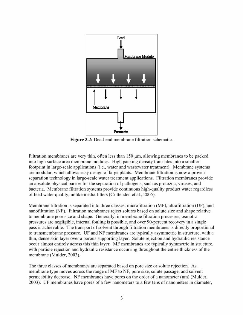
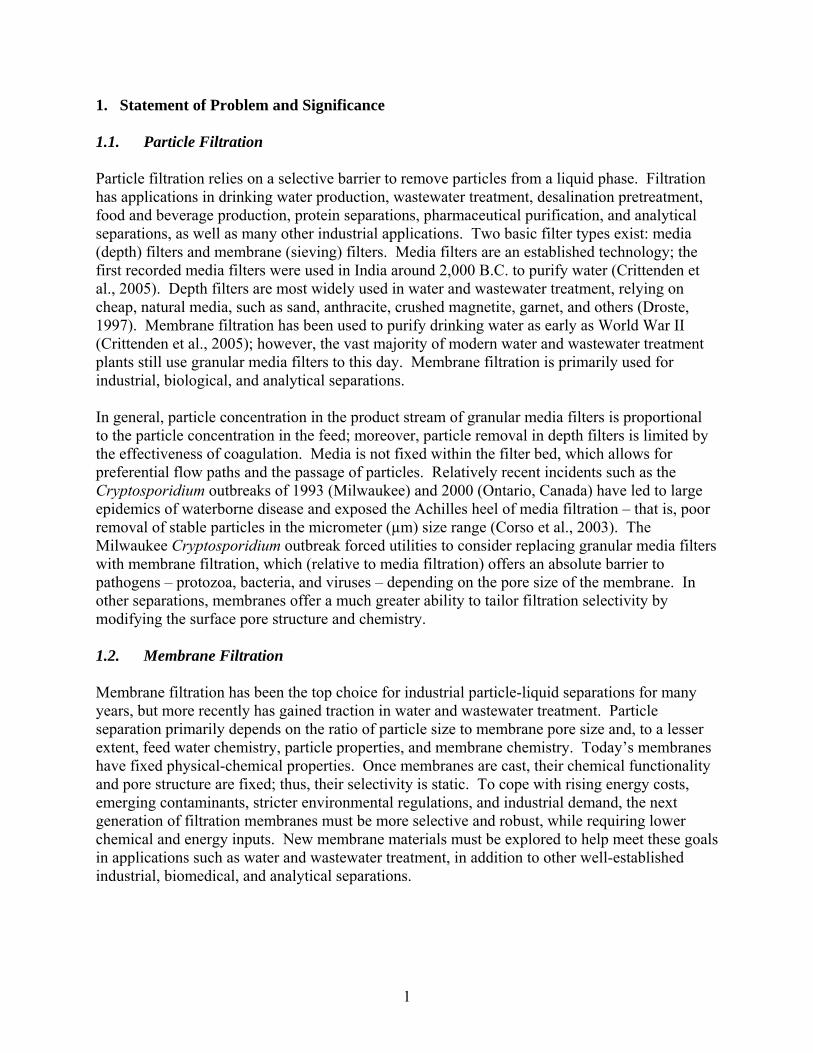
Figure 2.2: Dead-end membrane filtration schematic. Filtration membranes are very thin, often less than 150 µm, allowing membranes to be packed into high surface area membrane modules. High packing density translates into a smaller footprint in large-scale applications (i.e., water and wastewater treatment). Membrane systems are modular, which allows easy design of large plants. Membrane filtration is now a proven separation technology in large-scale water treatment applications. Filtration membranes provide an absolute physical barrier for the separation of pathogens, such as protozoa, viruses, and bacteria. Membrane filtration systems provide continuous high-quality product water regardless of feed water quality, unlike media filters (Crittenden et al., 2005). Membrane filtration is separated into three classes: microfiltration (MF), ultrafiltration (UF), and nanofiltration (NF). Filtration membranes reject solutes based on solute size and shape relative to membrane pore size and shape. Generally, in membrane filtration processes, osmotic pressures are negligible, internal fouling is possible, and over 90-percent recovery in a single pass is achievable. The transport of solvent through filtration membranes is directly proportional to transmembrane pressure. UF and NF membranes are typically asymmetric in structure, with a thin, dense skin layer over a porous supporting layer. Solute rejection and hydraulic resistance occur almost entirely across this thin layer. MF membranes are typically symmetric in structure, with particle rejection and hydraulic resistance occurring throughout the entire thickness of the membrane (Mulder, 2003). The three classes of membranes are separated based on pore size or solute rejection. As membrane type moves across the range of MF to NF, pore size, solute passage, and solvent permeability decrease. NF membranes have pores on the order of a nanometer (nm) (Mulder, 2003). UF membranes have pores of a few nanometers to a few tens of nanometers in diameter,

3

while MF membranes have pores ranging in diameter from 0.1 µm to several micrometers (Mulder, 2003). There is some overlap of solute rejection between MF, UF, and NF membranes, as shown in Figure 2.3.

Figure 2.3: Application range of MF, UF, NF, and reverse osmosis membranes (Mulder, 2003).

Membrane filtration processes are limited by several factors, including fixed selectivity, fouling, and degradation. Once they are fabricated, filtration membranes have fixed selectivity. It is difficult to adapt existing membrane processes to emerging contaminants without the addition of chemical agents or new membranes. Like all filtration processes, membrane filtration is prone to fouling. Filtration membranes can experience both internal and external fouling, which can occur on top of the membrane surface and within the pore structure, respectively. Membrane fouling increases energy consumption and operating costs in the forms of increased applied pressure, air scouring, cleaning chemicals, or other anti-fouling measures. Filtration membranes are cleaned by frequent hydraulic backwashing and periodic chemical washing to remove adsorbed foulants. These frequent process interruptions reduce productivity and create a residual waste stream. Repeated chemical cleaning can reduce membrane permeability and selectivity over time. Membrane integrity must be continuously monitored to ensure that membrane degradation has not compromised the filtration process.

4

2.2. Separation Mechanisms for Porous Filtration Membranes The main mechanisms by which particles are rejected by porous filtration membranes include: (1) size exclusion or sieving, (2) charge exclusion, and (3) specific chemical interactions. Depth filtration may play a minor role, but it is generally neglected due to the thin cross-section of a membrane. The capture of particles and solutes internally by a membrane leads to a rapid, often irreversible loss of permeability (see discussion below on fouling). Size exclusion is the dominant filtration mechanism. Particles larger than membrane pores are largely rejected, while much smaller particles mostly pass through. The transport of particles similar in size to membrane pores is more difficult to track and sensitive to additional factors. Real membranes exhibit a distribution of pore sizes and shapes. Solutes also vary in size, shape, and chemistry – sometimes dynamically. For example, solutes may be amphoteric or amphiphilic and can change shape when forced through a membrane pore. Ferry developed a model analogous to the interception mechanism in the isolated collector model for granular filtration to describe particle retention by pore exclusion (Crittenden et al., 2005; Ferry, 1936). However, this model does not account for attachment efficiency based on membrane-particle interfacial forces. Ferry’s model is based on the assumption that any particle contacting the membrane surface is retained. In laminar flow conditions, particles move parallel to streamlines towards cylindrical membrane pores. Particles impacting pore edges are rejected, while those that follow streamlines through the center of pores pass as shown in Figure 2.4.

Figure 2.4: Particle rejection mechanism, according to Ferry’s model.

5

According to the Ferry mechanical-sieving model, it is possible for particles smaller than the pore to be rejected. Particle passage (p) is a function of particle diameter (dp) relative to membrane pore diameter (dpore), according to (Wiesner and Buckley, 1996)

⎭⎬⎫

⎩⎨⎧

>≤−−−

=1;01;])1(2[)1( 22

λλλλ Gp , (2.1)

where λ = dp/dpore and G is the lag coefficient empirically determined by Zeman and Wales (1981) to be ( )27146.0exp λ−=G . (2.2) Pore size may be altered during the filtration process by pore blocking. Spherical particles larger than spherical pores (λ > 1) can cause complete pore blocking. Smaller non-spherical particles can partially block pores at the membrane surface or on the pore walls, resulting in pore restriction and altering the rejection properties of the membrane. However, this model cannot be taken literally as particles are not hard spheres. For example, flexible proteins can deform under stress and change shape as they pass through the pore of a membrane (Mulder, 2003). Filtration membranes may also reject or retain particles through various chemical interactions in two ways: 1) attraction and entrance into membrane pores; or 2) repulsion and exclusion from membrane pores (Probstein, 2003). Solute and membrane surface chemistries govern chemical exclusion, sometimes in combination with feed water chemistry. A universal attractive interaction derives from van der Waals forces. Temporary polarization caused by the constant movement of electrons or permanent dipoles result in an uneven distribution of charge between two species, which induces a long-range attractive force that decays as a function of separation distance up to about 10 nm. Beyond 10 nm, van der Waals forces decay as a function of the square of separation distance (Van Oss, 2003; Israelachvili, 1991). Van der Waals forces cause solutes to be drawn into pores and can lead to adsorption to both internal and external membrane surfaces. Coulombic interaction between particle and membrane surfaces is caused by the overlap of electrical double layers (Crittenden et al., 2005). This force is felt over a range of ~1 to ~100 nm, decays exponentially with distance, and is attractive when the particle and membrane are oppositely charge or repulsive when they are similarly charged (Van Oss, 2003). Coulombic interactions may be large enough to force particles into membrane pores or prevent particles from entering membrane pores (Deen, 1987; Causserand et al., 1996; Pujar and Zydney, 1994; Bhattacharjee et al., 1996). In high ionic strength solutions, the charge is negated and the electrical double layer is compressed. In the case of like-charged particles and membranes, the compression of electrical double layers allows particles to approach membrane surfaces at a closer distance before feeling electrostatic repulsion. In an aqueous solution, particle and membrane surface potentials further decrease as solution pH approaches the isoelectric point of either particle or membrane. As particles can approach membrane surfaces more closely (i.e., at separations less than ~10 nm),

6

short-range non-specific and specific interactions come into play. Hydrophilic particles may be excluded from a membrane pore or prevented from adhering to a membrane surface due to multiple layers of ordered water molecules that surround the particle. Adsorbed water layers are strongly bound to hydrophilic surfaces and do not allow surfaces to approach close enough for adhesion to occur because dehydration requires enormous energy. In contrast, hydrophobic particles may be forced onto membrane surfaces by water and, thus, be retained by filtration membranes by adsorbing to membrane surfaces (Van Oss, 2003). Depth filtration through the membrane cross-section is another mechanism for particle removal by filtration membranes. An oversimplified depiction of a filtration membrane pore is provided in Figure 2.4. In reality, filtration membrane pores are not cylindrical channels with uniform diameters running straight through the membrane cross-section. Pores are often interconnected and follow a tortuous path, which increases the effective pore length. Longer, more tortuous pores increase the chance of particle attachment to pore walls by diffusion or collision, as illustrated in Figure 2.5.

Figure 2.5: Particle capture mechanism in filtration of liquid solutions by depth microfilters. Four capture mechanisms are shown: simple sieving; electrostatic adsorption; inertial impact;

and Brownian diffusion (Baker, 2004). Captured particles are shown in dark grey. Winding pores cause abrupt changes in fluid flow direction. Dense particles are unable to follow streamlines due to inertial effects and may collide with membrane surfaces. Particles can then adsorb to pore walls due to polymer-particle affinity. 2.3. Analysis of Membrane Pore Size or Molecular Weight Cut-Off As stated earlier, membrane pore size is the dominant factor in determining the rejection

7

characteristics of a filtration membrane. The pore size of a filtration membrane can be described by the membrane’s ability to retain solutes or particles of a given molecular weight or size. The nominal molecular weight cut-off (MWCO) is the minimum solute molecular weight that is rejected by a membrane at least 90 percent, whereas the absolute MWCO is the minimum solute molecular weight that is completely rejected (Cheryan, 1998). The MWCO is determined by performing rejection tests using solutes or globular proteins of known molecular weight with the membrane of interest. These test solutes should ideally be soluble in water or in a mildly buffered solution, cover a wide range of sizes, and should not adsorb to the membrane surface. Solutes such as sodium chloride (MW = 58.5 Daltons [Da]) and glucose (MW = 180 Da) are commonly used to cover the low end of the molecular weight range. Large proteins such as immunoglobulins (MW > 900 kilo Daltons [kDa]) are used for rejection tests of high molecular weight solutes. Solutes with intermediate sizes/molecular weights are used to complete the molecular weight cut-off test. Several solutes with molecular weights near the membrane’s anticipated MWCO should be included in the analysis. A general relationship between membrane pore size or solute molecular weight and solute rejection is shown in Figure 2.6. The sharp curve (dashed line) in Figure 2.6 represents the pore size distribution of an ideal membrane. An ideal membrane has a very narrow pore size distribution, but such a perfect membrane has not yet been realized in practice (Cheryan, 1998). The MWCO for an ideal membrane is very sharp because of the narrow pore size distribution. Real membranes have broader pore size distributions and MWCOs.

Figure 2.6: Relationship between pore size, molecular weight of ideal solutes, and ratings of ideal and real membranes (Cheryan, 1998).

8

There is no standard method for characterizing solute rejection by filtration membranes. Several conditions should be standardized including trans-membrane pressure, test solutes, temperature, stirring rate or cross-flow velocity, solute concentration, buffer system, ratio of volume of test solution to membrane surface area, permeate-to-feed ratio, or membrane pretreatment. Cheryan (1998) recommends the following conditions:

1. Pressure of 100 kilo Pascal (kPa). 2. Temperature of 25°C. 3. Maximum possible mass transfer to minimize concentration polarization. 4. Low solute concentrations (e.g., 0.1 percent). 5. Individual solutes in water or mildly buffered solution. 6. Two-hundred milliliters (mL) of solution in a dead-end cell using 47- to 62-milimeter

(mm) diameter membranes (18 to 29 square centimeters [cm2] surface area). 7. Removal of less than 10 percent of the solution as permeate to avoid concentration effects. 8. The membrane should be new and clean.

Several commonly used test solutes are listed in Table 2.1.

Table 2.1: Common Test Solutes Used to Characterize UF Membranes (Baker, 2004)

2.4. Pressure-Driven Flow through Porous Filtration Membranes Several models have been developed in an attempt to relate membrane properties and operating conditions to fluid flow through porous membranes. Each model has its own shortcomings, many of which are due to non-ideal pore characteristics in real membranes. Fluid flow through membranes is induced by some driving force. In the case of filtration membranes, fluid flow is caused by a pressure difference across the membrane. The following is a general expression relating pressure to fluid flux:

9

dxdpAJv −= , (2.3)

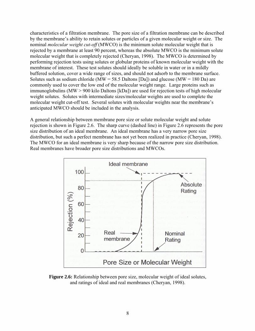
where Jv is fluid flux (volumetric flow per unit area), A is a phenomenological coefficient, p is pressure, and x is distance. This expression is further simplified by recalling that flow through porous filtration membranes is directly proportional to pressure. The following equation relates fluid flux to pressure drop with a permeability coefficient (Lp) pLJ pv Δ= . (2.4) In an ideal filtration membrane, pores are evenly distributed on the membrane surface, have uniform diameters, and pass straight through the membrane. The Hagen-Poiseuille model for flow through porous membranes assumes that an ideal membrane can be modeled as an array of straight, cylindrical channels, as depicted in Figure 2.7.

Figure 2.7: Membrane modeled as an array of cylindrical channels (left) and a pore with diameter, dp, and length (membrane thickness), l, (right).

It is assumed that the inter-channel space is a solid phase, which is impermeable to the fluid. This model relates applied pressure, pore diameter, porosity, and fluid viscosity to fluid flux. The model is derived by solving a momentum balance of flow through capillaries (Bird et al., 1960). The form of the Hagen-Poiseuille model most applicable to membrane filtration is given below (Cheryan, 1998)

pl

dJ p

v Δ=μ

ε32

2

, (2.5)

where ε is membrane porosity, dp is pore diameter, μ is fluid dynamic viscosity, l is membrane thickness, and ∆p is the applied trans-membrane pressure. If the filtration membrane is asymmetric (integrally skinned), then ε is surface porosity, l is membrane skin thickness, and ∆p is the pressure drop across the skin layer. A tortuosity term can be added to Equation 2.5 to help account for the winding flow paths often found in real membranes. The pore length, l, is multiplied by pore tortuosity, τ. Tortuosity is the ratio of real pore length to membrane thickness (symmetric membrane) or skin thickness (asymmetric membrane), lreal/∆x. Tortuosity may be approximated from membrane porosity by the following relation:

10

( )21ln ετ −= . (2.6) By expressing Equation 2.5 in terms of Lp and ∆p, it is apparent that membrane permeability is proportional to ε·dp

2·(τ·l)-1. Kozeny and Carman developed a model to describe laminar flow through porous media. In the Kozeny-Carman model, a porous filtration membrane is represented as a packed bed of spherical particles, as shown in Figure 2.8. Here, dp is the particle diameter and l is the membrane thickness. Membrane permeability according to the Kozeny-Carman model is expressed as

( ) lKSLp με

ε22

3

1−= , (2.7)

where ε is membrane porosity, K is the Kozeny coefficient, S is particle specific surface area, μ is fluid dynamic viscosity, and l is membrane thickness. The Kozeny coefficient has been found to vary with particle volume fraction as shown in Table 2.2.

Figure 2.8: Cross section of a filtration membrane modeled as a packed bed of spherical particles.

Table 2.2: Kozeny Coefficient as a Function of Particle Volume Fraction (Holdich, 2002)

11

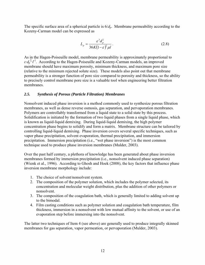
The specific surface area of a spherical particle is 6/dp. Membrane permeability according to the Kozeny-Carman model can be expressed as

( ) lK

dL p

p μεε

2

23

136 −= . (2.8)

As in the Hagen-Poiseuille model, membrane permeability is approximately proportional to ε·dp

2·l-1. According to the Hagen-Poiseuille and Kozeny-Carman models, an improved membrane should have maximum porosity, minimum thickness, and maximum pore size (relative to the minimum rejected solute size). These models also point out that membrane permeability is a stronger function of pore size compared to porosity and thickness, so the ability to precisely control membrane pore size is a valuable tool when engineering better filtration membranes. 2.5. Synthesis of Porous (Particle Filtration) Membranes Nonsolvent induced phase inversion is a method commonly used to synthesize porous filtration membranes, as well as dense reverse osmosis, gas separation, and pervaporation membranes. Polymers are controllably transformed from a liquid state to a solid state by this process. Solidification is initiated by the formation of two liquid phases from a single liquid phase, which is known as liquid-liquid demixing. During liquid-liquid demixing, the high polymer concentration phase begins to solidify and form a matrix. Membrane structure can be tailored by controlling liquid-liquid demixing. Phase inversion covers several specific techniques, such as vapor phase precipitation, solvent evaporation, thermal precipitation, and immersion precipitation. Immersion precipitation (i.e., “wet phase inversion”) is the most common technique used to produce phase inversion membranes (Mulder, 2003). Over the past half century, a plethora of knowledge has been generated about phase inversion membranes formed by immersion precipitation (i.e., nonsolvent induced phase separation) (Wienk et al., 1996). According to Ghosh and Hoek (2008), the key factors that influence phase inversion membrane morphology include:

1. The choice of solvent/nonsolvent system. 2. The composition of the polymer solution, which includes the polymer selected, its

concentration and molecular weight distribution, plus the addition of other polymers or nonsolvent.

3. The composition of the coagulation bath, which is generally limited to adding solvent up to the bimodal.

4. Film casting conditions such as polymer solution and coagulation bath temperature, film thickness, immersion in a nonsolvent with low mutual affinity to the solvent, or use of an evaporation step before immersing into the nonsolvent.

The latter two techniques of Item 4 (see above) are generally used to produce integrally skinned membranes for gas separation, vapor permeation, or pervaporation (Mulder, 2003).

12

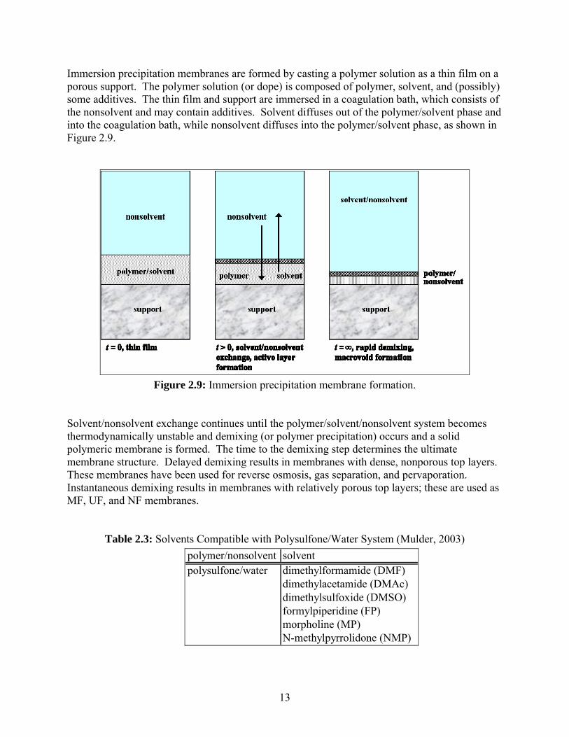
Immersion precipitation membranes are formed by casting a polymer solution as a thin film on a porous support. The polymer solution (or dope) is composed of polymer, solvent, and (possibly) some additives. The thin film and support are immersed in a coagulation bath, which consists of the nonsolvent and may contain additives. Solvent diffuses out of the polymer/solvent phase and into the coagulation bath, while nonsolvent diffuses into the polymer/solvent phase, as shown in Figure 2.9.

Figure 2.9: Immersion precipitation membrane formation. Solvent/nonsolvent exchange continues until the polymer/solvent/nonsolvent system becomes thermodynamically unstable and demixing (or polymer precipitation) occurs and a solid polymeric membrane is formed. The time to the demixing step determines the ultimate membrane structure. Delayed demixing results in membranes with dense, nonporous top layers. These membranes have been used for reverse osmosis, gas separation, and pervaporation. Instantaneous demixing results in membranes with relatively porous top layers; these are used as MF, UF, and NF membranes.

Table 2.3: Solvents Compatible with Polysulfone/Water System (Mulder, 2003)

polymer/nonsolvent solventpolysulfone/water dimethylformamide (DMF)

dimethylacetamide (DMAc)dimethylsulfoxide (DMSO)formylpiperidine (FP)morpholine (MP)N-methylpyrrolidone (NMP)

13

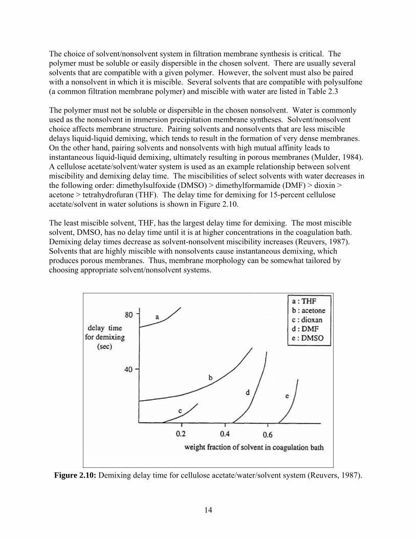
The choice of solvent/nonsolvent system in filtration membrane synthesis is critical. The polymer must be soluble or easily dispersible in the chosen solvent. There are usually several solvents that are compatible with a given polymer. However, the solvent must also be paired with a nonsolvent in which it is miscible. Several solvents that are compatible with polysulfone (a common filtration membrane polymer) and miscible with water are listed in Table 2.3 The polymer must not be soluble or dispersible in the chosen nonsolvent. Water is commonly used as the nonsolvent in immersion precipitation membrane syntheses. Solvent/nonsolvent choice affects membrane structure. Pairing solvents and nonsolvents that are less miscible delays liquid-liquid demixing, which tends to result in the formation of very dense membranes. On the other hand, pairing solvents and nonsolvents with high mutual affinity leads to instantaneous liquid-liquid demixing, ultimately resulting in porous membranes (Mulder, 1984). A cellulose acetate/solvent/water system is used as an example relationship between solvent miscibility and demixing delay time. The miscibilities of select solvents with water decreases in the following order: dimethylsulfoxide (DMSO) > dimethylformamide (DMF) > dioxin > acetone > tetrahydrofuran (THF). The delay time for demixing for 15-percent cellulose acetate/solvent in water solutions is shown in Figure 2.10. The least miscible solvent, THF, has the largest delay time for demixing. The most miscible solvent, DMSO, has no delay time until it is at higher concentrations in the coagulation bath. Demixing delay times decrease as solvent-nonsolvent miscibility increases (Reuvers, 1987). Solvents that are highly miscible with nonsolvents cause instantaneous demixing, which produces porous membranes. Thus, membrane morphology can be somewhat tailored by choosing appropriate solvent/nonsolvent systems.

Figure 2.10: Demixing delay time for cellulose acetate/water/solvent system (Reuvers, 1987).

14

Many different polymers are used in the synthesis of filtration membranes. Polymeric MF membranes are segregated into two classes: hydrophobic and hydrophilic. Hydrophobic MF membrane materials include poly(vinylidene fluoride) (PVDF), polyethylene (PE), polytetrafluoroethylene (PTFE, Teflon), and polypropylene (PP). Hydrophilic MF membrane materials include polycarbonate (PC), cellulose esters, polysulfone (PSf), poly(ether sulfone) (PES), polyetheretherketone (PEEK), aliphatic polyamides (PA), polyimides (PI), and poly(ether imide) (PEI) (Crittenden et al., 2005; Mulder, 2003). MF membranes are typically symmetric in structure. Porosity and pore structure are fairly homogenous throughout the thickness of MF membranes. UF membranes, however, have an asymmetric structure. UF membranes have a thin “skin” layer containing small pores. Below the skin layer are larger voids, as shown in Figure 2.11. Polymers traditionally used to make UF membranes include PVDF, cellulosics, PSf, PES, sulfonated PSf, PI, PEI, PEEK, polyacrylonitrile, and PA (Mulder, 2003). UF membranes are typically hydrophilic, as evidenced by the polymers used in their synthesis. Membrane hydrophilicity ultimately determines membrane permeability, fouling propensity, and solute rejection.

Figure 2.11: Asymmetric structure of a UF membrane (Crittenden et al., 2005). Polymer concentration in the dope solution is yet another parameter affecting membrane morphology. Typical polymer concentration ranges from 15 to 20 weight percent (Baker, 2004). Increasing polymer concentration in the polymer solution reduces the solvent volume in the polymer film. Polymer concentration is much higher at the film surface, which results in a denser top layer (Mosqueda-Jimenez et al., 2004). Instantaneous demixing can still occur, but the resulting membrane has lower porosity. The permeability of a polysulfone UF membrane as a function of polymer concentration is shown in Table 2.4. Membrane permeability decreases as polymer concentration increases (Chakrabarty et al., 2008a).

15

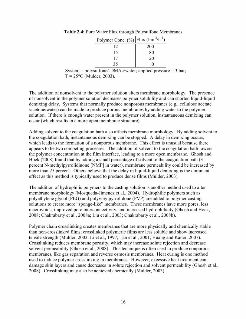
Table 2.4: Pure Water Flux through Polysulfone Membranes

Polymer Conc. (%) Flux (l·m-2·h-1)12 20015 8017 2035 0

System = polysulfone/-DMAc/water; applied pressure = 3 bar; T = 25°C (Mulder, 2003).

The addition of nonsolvent to the polymer solution alters membrane morphology. The presence of nonsolvent in the polymer solution decreases polymer solubility and can shorten liquid-liquid demixing delay. Systems that normally produce nonporous membranes (e.g., cellulose acetate /acetone/water) can be made to produce porous membranes by adding water to the polymer solution. If there is enough water present in the polymer solution, instantaneous demixing can occur (which results in a more open membrane structure).

Adding solvent to the coagulation bath also affects membrane morphology. By adding solvent to the coagulation bath, instantaneous demixing can be stopped. A delay in demixing occurs, which leads to the formation of a nonporous membrane. This effect is unusual because there appears to be two competing processes. The addition of solvent to the coagulation bath lowers the polymer concentration at the film interface, leading to a more open membrane. Ghosh and Hoek (2008) found that by adding a small percentage of solvent to the coagulation bath (3-percent N-methylpyrrolidinone [NMP] in water), membrane permeability could be increased by more than 25 percent. Others believe that the delay in liquid-liquid demixing is the dominant effect as this method is typically used to produce dense films (Mulder, 2003). The addition of hydrophilic polymers to the casting solution is another method used to alter membrane morphology (Mosqueda-Jimenez et al., 2004). Hydrophilic polymers such as polyethylene glycol (PEG) and polyvinylpyrrolidone (PVP) are added to polymer casting solutions to create more “sponge-like” membranes. These membranes have more pores, less macrovoids, improved pore interconnectivity, and increased hydrophilicity (Ghosh and Hoek, 2008; Chakrabarty et al., 2008a; Liu et al., 2003; Chakrabarty et al., 2008b). Polymer chain crosslinking creates membranes that are more physically and chemically stable than non-crosslinked films; crosslinked polymeric films are less soluble and show increased tensile strength (Mulder, 2003; Li et al., 1997; Tan et al., 2001; Huang and Kaner, 2007). Crosslinking reduces membrane porosity, which may increase solute rejection and decrease solvent permeability (Ghosh et al., 2008). This technique is often used to produce nonporous membranes, like gas separation and reverse osmosis membranes. Heat curing is one method used to induce polymer crosslinking in membranes. However, excessive heat treatment can damage skin layers and cause decreases in solute rejection and solvent permeability (Ghosh et al., 2008). Crosslinking may also be achieved chemically (Mulder, 2003).

16

2.6. Polyaniline Polymers traditionally used in the synthesis of filtration membranes are insulators. However, there is an emerging class of polymers that demonstrate appreciable electrical conductivity. Conducting polymers are an exciting prospective membrane material. Theoretically, an electrically conducting polymeric membrane might be dynamically selective by applying an external electrical potential across the membrane, thus inducing an electric field within membrane pores. The in-pore electric field should impact solute transport depending on the induced membrane charge relative to solute charge. The conducting properties of polyaniline were rediscovered in the early 1980s (Huang and Kaner, 2007) and have since been studied in numerous applications, including battery electrodes (Desilvestro et al., 1992), electromagnetic shielding devices (Joo and Epstein, 1994; Trivedi and Dhawan, 1993), and anticorrosion coatings (Yao et al., 2008; Alam et al., 2008; Lu et al., 1995). Interest in polyaniline has continued to grow due to its conducting properties, relatively simple synthesis, and the low cost of aniline (Feast et al., 1996). Early studies show that it may be possible to make thin films from polyaniline nanofibers with super-hydrophilic ordered pore structures, which makes this polymer an interesting candidate for use in filtration membrane synthesis. More on the use of polyaniline in the synthesis of filtration membranes will be shown and discussed in later sections. The chemical structure of polyaniline is shown in Figure 2.12.

Figure 2.12: Chemical structure of polyaniline (Feast et al., 1996). The chemical oxidative polymerization of aniline to polyaniline was first described by Letheby (1862) and further studied by Mohilner et al. (1962). Polyaniline can exist in a number of different oxidation states, as shown in Figure 2.13. The oxidation states range from fully reduced (leucoemeraldine) down to fully oxidized (pernigraniline). The fully reduced form of polyaniline is the leucoemeraldine oxidation state. Polyaniline in the emeraldine state has half of its nitrogens in the amine form and half in the imine form. Pernigraniline is the fully oxidized form of polyaniline. Unlike most conducting polymers, the fully oxidized form of polyaniline is non-conducting. A unique feature of polyaniline is that the intermediate oxidation state, the emeraldine state, is the only form of polyaniline capable of carrying charge (Feast et al., 1996). The emeraldine state of polyaniline becomes electrically conducting only when doped with a salt that protonates all imine nitrogens on the polymer backbone (Huang and Kaner, 2007). The undoped emeraldine base form of polyaniline has a conductivity below 10-10 Siemens per centimeter (S·cm-1), while doped emeraldine polyaniline has a conductivity on the order of 1 S·cm-1 (Huang et al., 1986). The conductivity of polyaniline containing water is five times higher than completely dry polyaniline (Feast et al., 1996).

17

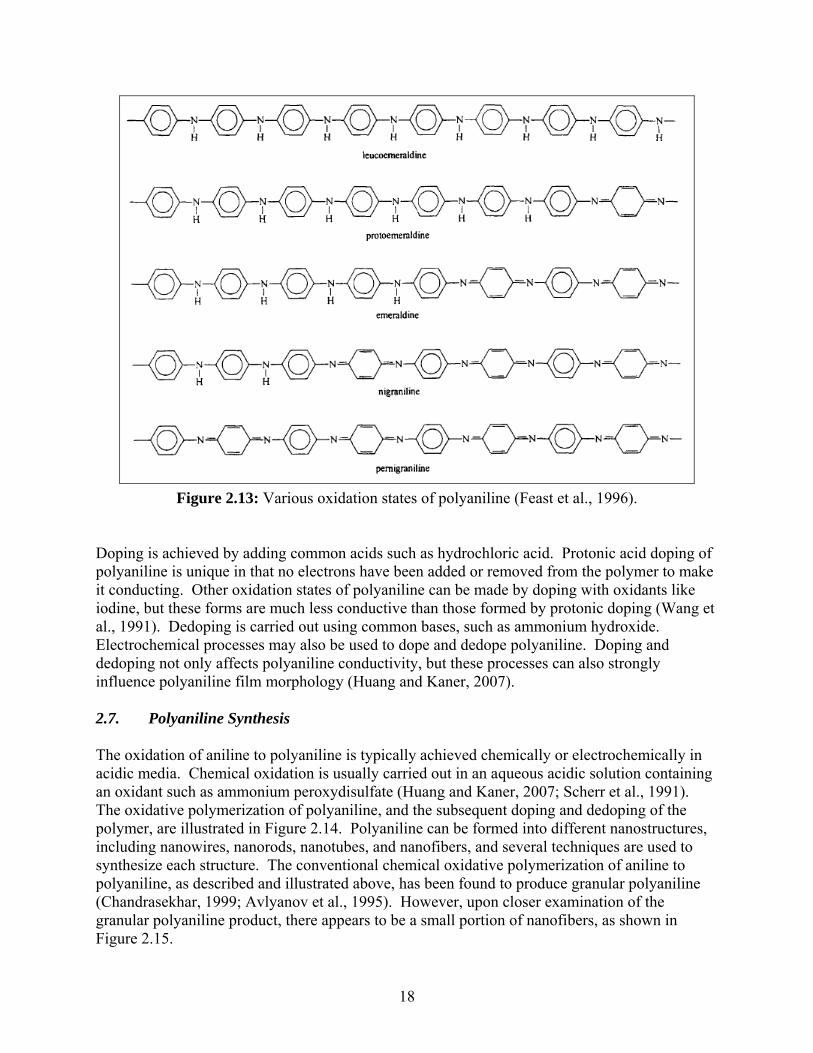
Figure 2.13: Various oxidation states of polyaniline (Feast et al., 1996). Doping is achieved by adding common acids such as hydrochloric acid. Protonic acid doping of polyaniline is unique in that no electrons have been added or removed from the polymer to make it conducting. Other oxidation states of polyaniline can be made by doping with oxidants like iodine, but these forms are much less conductive than those formed by protonic doping (Wang et al., 1991). Dedoping is carried out using common bases, such as ammonium hydroxide. Electrochemical processes may also be used to dope and dedope polyaniline. Doping and dedoping not only affects polyaniline conductivity, but these processes can also strongly influence polyaniline film morphology (Huang and Kaner, 2007). 2.7. Polyaniline Synthesis The oxidation of aniline to polyaniline is typically achieved chemically or electrochemically in acidic media. Chemical oxidation is usually carried out in an aqueous acidic solution containing an oxidant such as ammonium peroxydisulfate (Huang and Kaner, 2007; Scherr et al., 1991). The oxidative polymerization of polyaniline, and the subsequent doping and dedoping of the polymer, are illustrated in Figure 2.14. Polyaniline can be formed into different nanostructures, including nanowires, nanorods, nanotubes, and nanofibers, and several techniques are used to synthesize each structure. The conventional chemical oxidative polymerization of aniline to polyaniline, as described and illustrated above, has been found to produce granular polyaniline (Chandrasekhar, 1999; Avlyanov et al., 1995). However, upon closer examination of the granular polyaniline product, there appears to be a small portion of nanofibers, as shown in Figure 2.15.

18

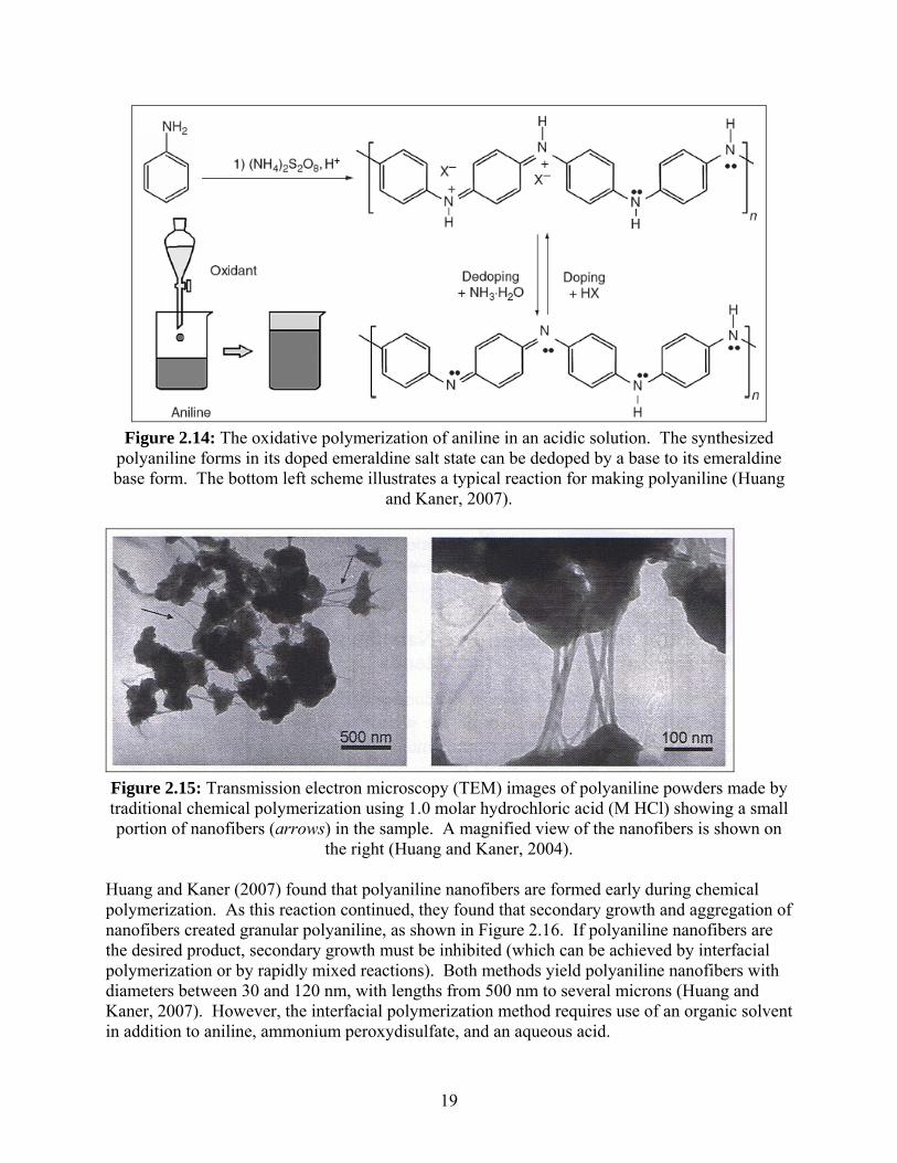
Figure 2.14: The oxidative polymerization of aniline in an acidic solution. The synthesized polyaniline forms in its doped emeraldine salt state can be dedoped by a base to its emeraldine base form. The bottom left scheme illustrates a typical reaction for making polyaniline (Huang

and Kaner, 2007).

Figure 2.15: Transmission electron microscopy (TEM) images of polyaniline powders made by traditional chemical polymerization using 1.0 molar hydrochloric acid (M HCl) showing a small portion of nanofibers (arrows) in the sample. A magnified view of the nanofibers is shown on

the right (Huang and Kaner, 2004). Huang and Kaner (2007) found that polyaniline nanofibers are formed early during chemical polymerization. As this reaction continued, they found that secondary growth and aggregation of nanofibers created granular polyaniline, as shown in Figure 2.16. If polyaniline nanofibers are the desired product, secondary growth must be inhibited (which can be achieved by interfacial polymerization or by rapidly mixed reactions). Both methods yield polyaniline nanofibers with diameters between 30 and 120 nm, with lengths from 500 nm to several microns (Huang and Kaner, 2007). However, the interfacial polymerization method requires use of an organic solvent in addition to aniline, ammonium peroxydisulfate, and an aqueous acid.

19

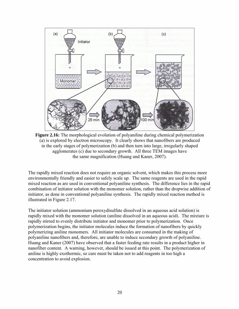
Figure 2.16: The morphological evolution of polyaniline during chemical polymerization (a) is explored by electron microscopy. It clearly shows that nanofibers are produced in the early stages of polymerization (b) and then turn into large, irregularly shaped

agglomerates (c) due to secondary growth. All three TEM images have the same magnification (Huang and Kaner, 2007).

The rapidly mixed reaction does not require an organic solvent, which makes this process more environmentally friendly and easier to safely scale up. The same reagents are used in the rapid mixed reaction as are used in conventional polyaniline synthesis. The difference lies in the rapid combination of initiator solution with the monomer solution, rather than the dropwise addition of initiator, as done in conventional polyaniline synthesis. The rapidly mixed reaction method is illustrated in Figure 2.17. The initiator solution (ammonium peroxydisulfate dissolved in an aqueous acid solution) is rapidly mixed with the monomer solution (aniline dissolved in an aqueous acid). The mixture is rapidly stirred to evenly distribute initiator and monomer prior to polymerization. Once polymerization begins, the initiator molecules induce the formation of nanofibers by quickly polymerizing aniline monomers. All initiator molecules are consumed in the making of polyaniline nanofibers and, therefore, are unable to induce secondary growth of polyaniline. Huang and Kaner (2007) have observed that a faster feeding rate results in a product higher in nanofiber content. A warning, however, should be issued at this point. The polymerization of aniline is highly exothermic, so care must be taken not to add reagents in too high a concentration to avoid explosion.

20

Figure 2.17: Schematic illustration showing a rapidly mixed reaction in which (a) the initiator and monomer solutions are rapidly mixed together all at once. Therefore, (b) and (c), the

initiator molecules, are depleted during the formation of nanofibers, disabling further polymerization that leads to overgrowth. Pure nanofibers are obtained, as shown

in the scanning electron microscopy (SEM) image (Huang and Kaner, 2007). Polyaniline nanofibers are recovered by filtration and washed with a series of solutions. The washed polymer is then dried. Polyaniline is soluble in the following:

• N,N-dimethylformamide (DMF) (Xia et al., 1995; Jing et al., 2007). • N-methylpyrrolidinone (NMP) (Jing et al., 2007; Virji et al., 2004; Angelopoulos et al.,

1997). • Tetrahydrofuran (THF) (Jing et al., 2007). • Dimethylsulfoxide (DMSO) (Jing et al., 2007). • Chloroform (Xia et al., 1995). • Benzyl alcohol (Xia et al., 1995). • Hexafluoroisopropanol (HFIP) (Virji et al., 2004; Hopkins et al., 1996). • m-Cresol (Matveeva et al., 1996). • p-Cresol (Xia et al., 1995). • 2-Chlorophenol and 2-fluorophenol (Xia et al., 1995). • 3-Ethylphenol (Xia et al., 1995). • Formic acid (Hatchett et al., 1999).

Polyaniline nanofiber solubility has been shown to be greater than granular polyaniline in NMP, DMF, DMSO, and THF (Jing et al., 2007). If polyaniline nanofibers remain intact in the polymer solution, then the polymer nanostructure may be an important factor in determining membrane pore structure.

21

3. Preliminary Work 3.1. Polyaniline Membrane Synthesis and Characterization Polyaniline nanofibers were synthesized, as described above. Polyaniline-polysulfone (PANI-PSf) blend polymer solutions were created using NMP as the solvent. All polymer solutions were 18 percent by weight. Polymer solution composition ranged from pure polyaniline (1:0 PANI:PSf w/w) to pure polysulfone (0:1 PANI:PSf w/w), including intermediate compositions (3:1, 1:1, 1:3 PANI:PSf w/w). Films were cast on commercial nonwoven polyester fabric supports. Casting blade height (film thickness) was set at 152 µm using a feeler gauge. Room temperature deionized (DI) water was used as the nonsolvent. Films were immediately placed in the coagulation bath after casting, where they were allowed to soak one hour before the water was replaced. This cycle was repeated until a total of four washes were completed. Membranes were stored in deionized water overnight before testing. 3.1.1. Membrane Thickness, Pure Water Permeability, and SiO2 Rejection Membrane thickness, pure water permeability, and silica nanoparticle rejection results for polyaniline-polysulfone blend membranes are given in Table 3.1. Permeability and rejection tests were conducted in a Sterlitech dead-end flow cell. Silica nanoparticles (SNOWTEX-20L, Nissan Chemical Industries, Ltd.) with diameters of 40 nm were used as test particles. Nanoparticle concentration was measured using a turbidimeter (2100AN Turbidimeter, Hach Company). Permeability and rejection tests were repeated at least three times for each membrane, with the exception of 1:0, 1:1, and 0:1 membranes, which were repeated five times. Permeabilities and rejections for these membranes are presented in Figure 3.1.

Table 3.1: Polyaniline-Polysulfone Blend Membrane Thickness, Pure Water Permeability, and 40-nm Silica Rejection

Membrane [PANI :PSf w/w] PANI%:PSf%

Thickness [µm]

Std. Dev.

# Replicates

Std. Dev.

# Replicates

1:0 100 to 0 110 157.36 ± 24 5 85.90 ± 12.1% 43:1 75 to 25 130 33.60 ± 21 3 96.01 ± 2.4% 31:1 50 to 50 130 24.98 ± 4.5 5 99.50 ± 0.2% 51:3 25 to 75 130 25.35 ± 6.3 3 99.25 ± 0.4% 30:1 0 to 100 135 16.21 ± 1.3 5 99.44 ± 0.2% 5

Avg. Perm. [gfd/psi]

40 nm SiO2

Rejection

Water permeability shows a slight increase with increasing polyaniline content. However, the water permeability of pure polyaniline membranes is nearly an order of magnitude greater than for pure polysulfone membranes. Rejection is slightly lower in pure polyaniline membranes compared to pure polysulfone membranes. Results are consistent for membranes with low polyaniline content (1:1, 1:3, and 0:1); however, there is considerable error in the permeability and rejection data for pure polyaniline membranes. DI water contact angle measurements were conducted on 1:0, 1:1, and 0:1 membranes. Two sets of membranes were tested: “doped” and “undoped.” “Doped” membranes were soaked in pH 2

22

sulfuric acid (H2SO4) solution for 30 minutes prior to drying. “Undoped” membranes were taken straight from their deionized water storage bottles. All membranes were placed in a desiccator and allowed to dry overnight before testing. Results are presented in Table 3.2.

Figure 3.1: Permeability and rejection for PANI-PSf blended membranes.

Table 3.2: Water Contact Angles on PANI-PSf Membranes

Membrane (PANI:PSf w/w) CAavg Std. Dev.

1:0 0.0 0.01:1 34.0 37.30:1 74.4 2.81:0 0.0 0.01:1 0.0 0.00:1 80.7 3.4

Doped

Undoped

Both forms (doped and undoped) of the pure PANI membrane have an equilibrium DI water contact angle of 0°. The DI water drop appeared to be pulled into the membrane rather than spread over the surface. Video of this event showed the drop completely disappear in 15 to 20 seconds. There was little observable difference between the doped and undoped forms of the pure polysulfone membranes. However, the 1:1 membranes seemed to suffer from heterogeneities. Several spots on the doped 1:1 membrane were relatively hydrophobic (contact angle >60°), while regions a few centimeters away showed 0° equilibrium contact angles. Each

23

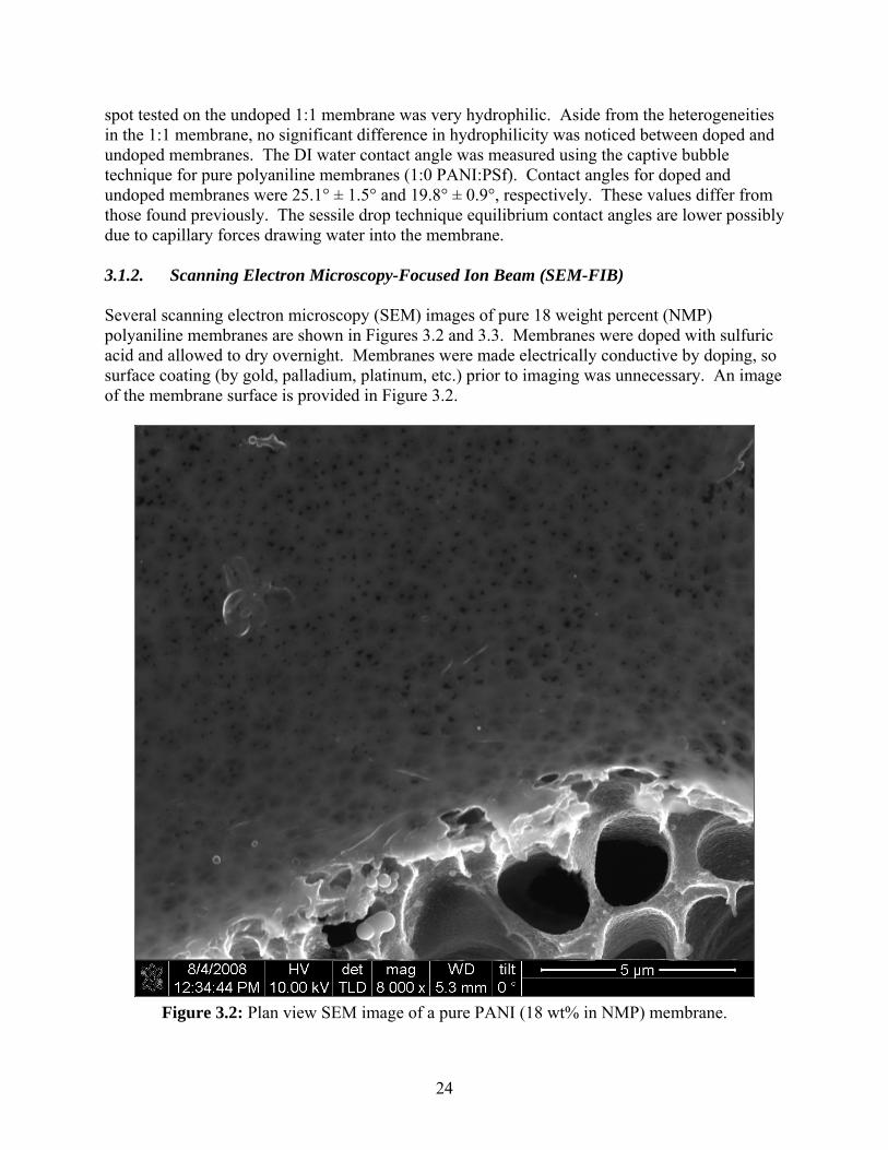
spot tested on the undoped 1:1 membrane was very hydrophilic. Aside from the heterogeneities in the 1:1 membrane, no significant difference in hydrophilicity was noticed between doped and undoped membranes. The DI water contact angle was measured using the captive bubble technique for pure polyaniline membranes (1:0 PANI:PSf). Contact angles for doped and undoped membranes were 25.1° ± 1.5° and 19.8° ± 0.9°, respectively. These values differ from those found previously. The sessile drop technique equilibrium contact angles are lower possibly due to capillary forces drawing water into the membrane. 3.1.2. Scanning Electron Microscopy-Focused Ion Beam (SEM-FIB) Several scanning electron microscopy (SEM) images of pure 18 weight percent (NMP) polyaniline membranes are shown in Figures 3.2 and 3.3. Membranes were doped with sulfuric acid and allowed to dry overnight. Membranes were made electrically conductive by doping, so surface coating (by gold, palladium, platinum, etc.) prior to imaging was unnecessary. An image of the membrane surface is provided in Figure 3.2.

Figure 3.2: Plan view SEM image of a pure PANI (18 wt% in NMP) membrane.

24

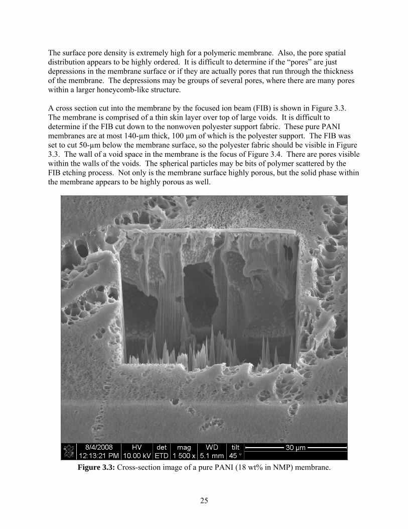
The surface pore density is extremely high for a polymeric membrane. Also, the pore spatial distribution appears to be highly ordered. It is difficult to determine if the “pores” are just depressions in the membrane surface or if they are actually pores that run through the thickness of the membrane. The depressions may be groups of several pores, where there are many pores within a larger honeycomb-like structure. A cross section cut into the membrane by the focused ion beam (FIB) is shown in Figure 3.3. The membrane is comprised of a thin skin layer over top of large voids. It is difficult to determine if the FIB cut down to the nonwoven polyester support fabric. These pure PANI membranes are at most 140-µm thick, 100 µm of which is the polyester support. The FIB was set to cut 50-µm below the membrane surface, so the polyester fabric should be visible in Figure 3.3. The wall of a void space in the membrane is the focus of Figure 3.4. There are pores visible within the walls of the voids. The spherical particles may be bits of polymer scattered by the FIB etching process. Not only is the membrane surface highly porous, but the solid phase within the membrane appears to be highly porous as well.

Figure 3.3: Cross-section image of a pure PANI (18 wt% in NMP) membrane.

25

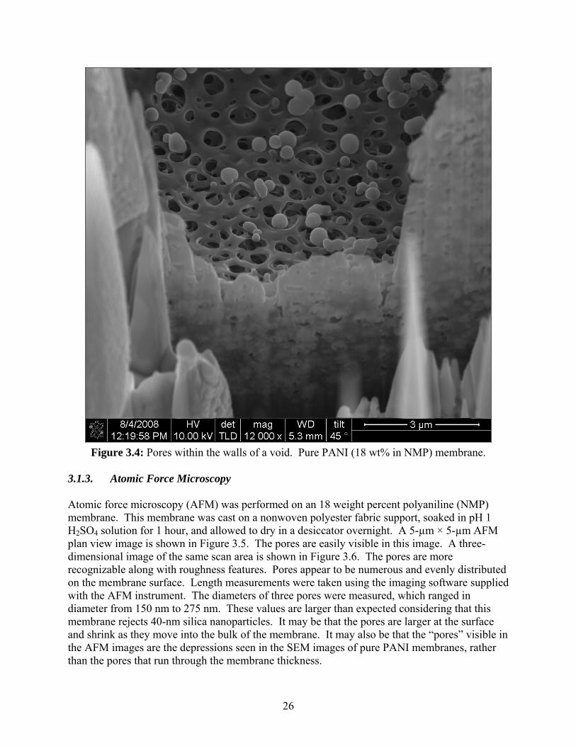
Figure 3.4: Pores within the walls of a void. Pure PANI (18 wt% in NMP) membrane. 3.1.3. Atomic Force Microscopy Atomic force microscopy (AFM) was performed on an 18 weight percent polyaniline (NMP) membrane. This membrane was cast on a nonwoven polyester fabric support, soaked in pH 1 H2SO4 solution for 1 hour, and allowed to dry in a desiccator overnight. A 5-µm × 5-µm AFM plan view image is shown in Figure 3.5. The pores are easily visible in this image. A three-dimensional image of the same scan area is shown in Figure 3.6. The pores are more recognizable along with roughness features. Pores appear to be numerous and evenly distributed on the membrane surface. Length measurements were taken using the imaging software supplied with the AFM instrument. The diameters of three pores were measured, which ranged in diameter from 150 nm to 275 nm. These values are larger than expected considering that this membrane rejects 40-nm silica nanoparticles. It may be that the pores are larger at the surface and shrink as they move into the bulk of the membrane. It may also be that the “pores” visible in the AFM images are the depressions seen in the SEM images of pure PANI membranes, rather than the pores that run through the membrane thickness.

26

Figure 3.5: Plan view AFM image of a pure PANI (18 wt% in NMP) membrane.

Figure 3.6: Three dimensional AFM image of a pure PANI (18 wt% in NMP) membrane.

27

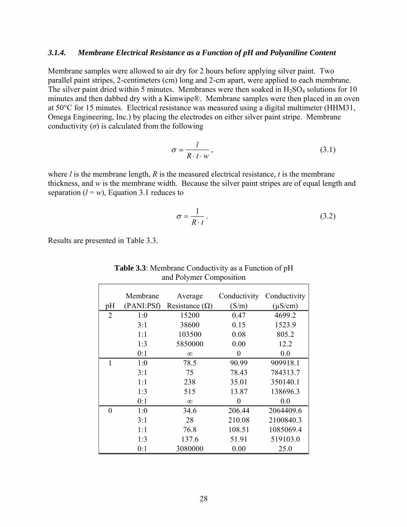
3.1.4. Membrane Electrical Resistance as a Function of pH and Polyaniline Content Membrane samples were allowed to air dry for 2 hours before applying silver paint. Two parallel paint stripes, 2-centimeters (cm) long and 2-cm apart, were applied to each membrane. The silver paint dried within 5 minutes. Membranes were then soaked in H2SO4 solutions for 10 minutes and then dabbed dry with a Kimwipe®. Membrane samples were then placed in an oven at 50°C for 15 minutes. Electrical resistance was measured using a digital multimeter (HHM31, Omega Engineering, Inc.) by placing the electrodes on either silver paint stripe. Membrane conductivity (σ) is calculated from the following

wtR

l⋅⋅

=σ , (3.1)

where l is the membrane length, R is the measured electrical resistance, t is the membrane thickness, and w is the membrane width. Because the silver paint stripes are of equal length and separation (l = w), Equation 3.1 reduces to

tR ⋅

=1σ . (3.2)

Results are presented in Table 3.3.

Table 3.3: Membrane Conductivity as a Function of pH and Polymer Composition

pHMembrane (PANI:PSf)

Average Resistance (Ω)

Conductivity (S/m)

Conductivity (µS/cm)

2 1:0 15200 0.47 4699.23:1 38600 0.15 1523.91:1 103500 0.08 805.21:3 5850000 0.00 12.20:1 ∞ 0 0.0

1 1:0 78.5 90.99 909918.13:1 75 78.43 784313.71:1 238 35.01 350140.11:3 515 13.87 138696.30:1 ∞ 0 0.0

0 1:0 34.6 206.44 2064409.63:1 28 210.08 2100840.31:1 76.8 108.51 1085069.41:3 137.6 51.91 519103.00:1 3080000 0.00 25.0

28

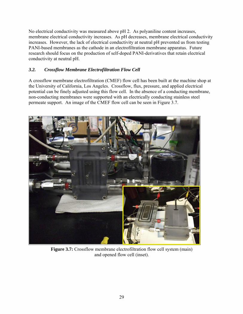
No electrical conductivity was measured above pH 2. As polyaniline content increases, membrane electrical conductivity increases. As pH decreases, membrane electrical conductivity increases. However, the lack of electrical conductivity at neutral pH prevented us from testing PANI-based membranes as the cathode in an electrofiltration membrane apparatus. Future research should focus on the production of self-doped PANI-derivatives that retain electrical conductivity at neutral pH. 3.2. Crossflow Membrane Electrofiltration Flow Cell A crossflow membrane electrofiltration (CMEF) flow cell has been built at the machine shop at the University of California, Los Angeles. Crossflow, flux, pressure, and applied electrical potential can be finely adjusted using this flow cell. In the absence of a conducting membrane, non-conducting membranes were supported with an electrically conducting stainless steel permeate support. An image of the CMEF flow cell can be seen in Figure 3.7.

Figure 3.7: Crossflow membrane electrofiltration flow cell system (main) and opened flow cell (inset).

29

3.3. Electrofiltration Using Polysulfone Membrane with Porous Stainless Steel Permeate Support

3.3.1. Constant Potential Electrofiltration experiments were performed using 18 wt% polysulfone (in NMP) membranes supported by a steel permeate spacer. Temperature was held constant at 25°C, and the pH was unadjusted (~5.4). SNOWTEX 20-L silica nanoparticles (dp = 40 to 50 nm) were added to the feed water at a concentration of 200 milligrams per liter (mg/L). The electrofiltration system operated with a constant flux of 40 gallons per square foot per day (gfd) and a constant Reynolds number of 112. Feed and permeate turbidity, pH, and conductivity were measured throughout the experiments. The development of normalized transmembrane pressure over time is plotted in Figure 3.8 for different electric field strengths.

Figure 3.8: Normalized transmembrane pressure over time for different field strengths. Experiments were performed using constant applied electrical field strengths of 0, 1, 10, and 100 Volts per centimeter (V/cm). There was little effect on transmembrane pressure drop when the electric field strength was 10 V/cm or lower. When a field strength of 100 V/cm was applied, the transmembrane pressure showed little increase over time, indicating a decrease in fouling rate. An additional experiment was performed at pH 9.5 with a field strength of 10 V/cm to see if an increase in particle zeta potential had an effect on particle mobility. Transmembrane pressure increased over time, which indicated that the fouling rate was similar to the experiment conducted at unadjusted pH and 10 V/cm.

30

Silica nanoparticle rejection measured over the course of these experiments is plotted in Figure 3.9. There was little difference in silica rejection beyond 3 hours, after which rejection was greater than 99 percent for all applied field strengths, with the exception of the experiment conducted at pH 9.5. The particles may be more stable at this high pH and thus may be less prone to form aggregates, which may result in increased passage of primary particles or smaller aggregates. The high rejections after 3 hours probably resulted from membrane fouling. Once a particle cake layer accumulated over the membrane surface, the rejection was largely by the particle cake layer rather than the membrane. The initial rejections suggest the magnitude of the applied voltage determined the rejection for 0, 1, and 10 V/cm, but at 100 V/cm, the rejection was very low. The membrane appeared damaged when it was removed from the filtration apparatus after exposure to 100 V/cm, potentially due to the extreme heat generated by the high applied voltage, as well as the electrochemical reactions generated by the associated high current density.

Figure 3.9: Silica nanoparticle rejection over time for different constant field strengths. 3.3.2. Pulsed Potential Experiments were performed using pulsed applied electrical potentials of 0, 1, 2, 5, 10, and 50 Volts (V). A commercial UF membrane (MX50, GE-Osmonics) was supported by a stainless steel permeate spacer. Pressure was maintained at 13 pounds per square inch (psi). As shown in Figure 3.10, there was little effect on flux when the electrical potential was lower than 50 V. When a potential of 50 V was applied, the flux rapidly increased, indicating a decrease in fouling

31

rate. Flux quickly declined once the potential was decreased. Silica nanoparticle rejection increased slightly over time and did not appear to be affected by the applied electrical potential. An additional experiment was conducted to see if there are any effects of a pulsed electric field on the transmembrane pressure of an already-fouled membrane. This experiment was conducted after the pH 9.5, E = 10 V/cm experiment discussed in Section 3.3.1, so all of the operating parameters are identical. Electrical pulses of 10, 50, 100, 250, and 500 V/cm were applied for two minutes each. Transmembrane pressure and field strengths are plotted over time in Figure 3.11.

Figure 3.10: Silica nanoparticle rejection and permeate flux over time for pulsed field strengths. No response in transmembrane pressure was detected for a field strength of 10 V/cm. Field strengths above 10 V/cm showed an increasing response in transmembrane pressure. As the pulsed electrical potential increased, the transmembrane pressure decreased. However, once the potential was turned off, the transmembrane pressure returned to the original value of about 1.5 psi. In the case of 250 and 500 V/cm, the transmembrane pressure returned to a slightly higher value of 1.6 and 1.7 psi, respectively.

32

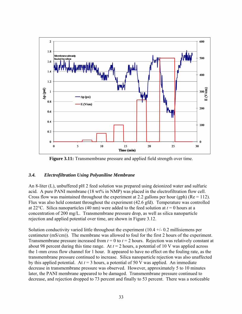
Figure 3.11: Transmembrane pressure and applied field strength over time.

3.4. Electrofiltration Using Polyaniline Membrane An 8-liter (L), unbuffered pH 2 feed solution was prepared using deionized water and sulfuric acid. A pure PANI membrane (18 wt% in NMP) was placed in the electrofiltration flow cell. Cross flow was maintained throughout the experiment at 2.2 gallons per hour (gph) (Re = 112). Flux was also held constant throughout the experiment (42.6 gfd). Temperature was controlled at 22°C. Silica nanoparticles (40 nm) were added to the feed solution at t = 0 hours at a concentration of 200 mg/L. Transmembrane pressure drop, as well as silica nanoparticle rejection and applied potential over time, are shown in Figure 3.12. Solution conductivity varied little throughout the experiment (10.4 +/- 0.2 millisiemens per centimeter (mS/cm)). The membrane was allowed to foul for the first 2 hours of the experiment. Transmembrane pressure increased from t = 0 to t = 2 hours. Rejection was relatively constant at about 98 percent during this time range. At t = 2 hours, a potential of 10 V was applied across the 1-mm cross flow channel for 1 hour. It appeared to have no effect on the fouling rate, as the transmembrane pressure continued to increase. Silica nanoparticle rejection was also unaffected by this applied potential. At t = 3 hours, a potential of 50 V was applied. An immediate decrease in transmembrane pressure was observed. However, approximately 5 to 10 minutes later, the PANI membrane appeared to be damaged. Transmembrane pressure continued to decrease, and rejection dropped to 73 percent and finally to 53 percent. There was a noticeable

33

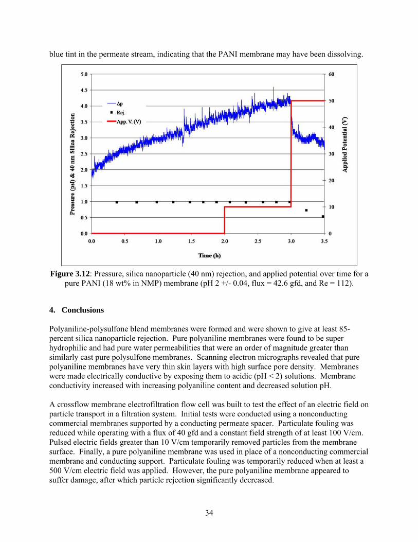
blue tint in the permeate stream, indicating that the PANI membrane may have been dissolving.

Figure 3.12: Pressure, silica nanoparticle (40 nm) rejection, and applied potential over time for a pure PANI (18 wt% in NMP) membrane (pH 2 +/- 0.04, flux = 42.6 gfd, and Re = 112).

4. Conclusions Polyaniline-polysulfone blend membranes were formed and were shown to give at least 85-percent silica nanoparticle rejection. Pure polyaniline membranes were found to be super hydrophilic and had pure water permeabilities that were an order of magnitude greater than similarly cast pure polysulfone membranes. Scanning electron micrographs revealed that pure polyaniline membranes have very thin skin layers with high surface pore density. Membranes were made electrically conductive by exposing them to acidic (pH < 2) solutions. Membrane conductivity increased with increasing polyaniline content and decreased solution pH. A crossflow membrane electrofiltration flow cell was built to test the effect of an electric field on particle transport in a filtration system. Initial tests were conducted using a nonconducting commercial membranes supported by a conducting permeate spacer. Particulate fouling was reduced while operating with a flux of 40 gfd and a constant field strength of at least 100 V/cm. Pulsed electric fields greater than 10 V/cm temporarily removed particles from the membrane surface. Finally, a pure polyaniline membrane was used in place of a nonconducting commercial membrane and conducting support. Particulate fouling was temporarily reduced when at least a 500 V/cm electric field was applied. However, the pure polyaniline membrane appeared to suffer damage, after which particle rejection significantly decreased.

34

Particle transport can be controlled by tuning the applied electric field across a membrane feed channel with the aid of an electrically conducting polymeric membrane. However, additional work must be done to find a polymer that is conductive in the pH 6 to 8 range and can withstand high current densities.

35

5. References Alam, J., U. Riaz, and S. Ahmad, “Development of nanostructured polyaniline dispersed smart

anticorrosive composite coatings,” Polymers for Advanced Technologies, 19 (2008) 882-888.

Angelopoulos, M., R. Dipietro, W.G. Zheng, A.G. MacDiarmid, and A.J. Epstein, “Effect of

selected processing parameters on solution properties and morphology of polyaniline and impact on conductivity,” Synthetic Metals, 84 (1997) 35-39.

Avlyanov, J.K., J.Y. Josefowicz, and A.G. Macdiarmid, “Atomic-force microscopy surface-

morphology studies of in-situ deposited polyaniline thin-films,” Synthetic Metals, 73 (1995) 205-208.

Baker, R.W., Membrane technology and applications, 2nd ed., John Wiley & Sons, Ltd, New

York, New York, 2004. Bhattacharjee, S., A. Sharma, and P.K. Bhattacharya, “Estimation and influence of long range

solute. Membrane interactions in ultrafiltration,” Industrial & Engineering Chemistry Research, 35 (1996) 3108-3121.

Bird, R.B., W.E. Stewart, and E.N. Lightfoot, Transport phenomena, Wiley, New York, NY,

1960. Causserand, C., M. Meireles, and P. Aimar, “Proteins transport through charged porous

membranes,” Chemical Engineering Research & Design, 74 (1996) 113-122. Chakrabarty, B. A.K. Ghoshal, and M.K. Purkait, “Preparation, characterization and

performance studies of polysulfone membranes using PVP as an additive,” Journal of Membrane Science, 315 (2008a) 36-47.

Chakrabarty, B., A.K. Ghoshal, and M.K. Purkait, “Effect of molecular weight of PEG on

membrane morphology and transport properties,” Journal of Membrane Science, 309 (2008b) 209-221.

Cheryan, M., Ultrafiltration and microfiltration handbook, Technomic Publishing Company,

Inc., Lancaster, PA, 1998. Corso, P.S., M.H. Kramer, K.A. Blair, D.G. Addiss, J.P. Davis, A.C. Haddix, “Cost of illness in

the 1993 waterborne cryptosporidium outbreak, Milwaukee, Wisconsin,” Emerging Infectious Diseases, 9 (2003) 426-431.

Crittenden, J.C., R.R. Trussell, D.W. Hand, K.J. Howe, and G. Tchobanoglous, Water treatment:

Principles and design, 2nd, John Wiley & Sons, Inc., Hoboken, New Jersey, 2005.

36

Deen, W.M., “Hindered transport of large molecules in liquid-filled pores,” Aiche Journal, 33 (1987) 1409-1425.

Desilvestro, J., W. Scheifele, and O. Haas, “In situ determination of gravimetric and volumetric

charge-densities of battery electrodes - polyaniline in aqueous and nonaqueous electrolytes,” Journal of the Electrochemical Society, 139 (1992) 2727-2736.

Droste, R.L., Theory and practice of water and wastewater treatment, John Wiley & Sons, Inc.,

New York, New York, 1997. Feast, W.J., J. Tsibouklis, K.L. Pouwer, L. Groenendaal, and E.W. Meijer, “Synthesis,

processing and material properties of conjugated polymers,” Polymer, 37 (1996) 5017-5047.

Ferry, J.D., “Statistical evaluation of sieve constants in ultrafiltration,” Journal of General

Physiology, 20 (1936) 95-104. Ghosh, A.K., and E.M.V. Hoek, “Impact of support membrane structure and chemistry on

polyamide reverse osmosis membrane properties,” Separation & Purification, (2008) submitted.

Ghosh, A.K., B.H. Jeong, X.F. Huang, and E.M.V. Hoek, “Impacts of reaction and curing

conditions on polyamide composite reverse osmosis membrane properties,” Journal of Membrane Science, 311 (2008) 34-45.

Hatchett, D.W, M. Josowicz, and J. Janata, “Acid doping of polyaniline: Spectroscopic and

electrochemical studies,” Journal of Physical Chemistry B, 103 (1999) 10992-10998. Holdich, R., Fundamentals of particle technology, Midland Information Technology &

Publishing, UK, 2002. Hopkins, A.R., P.G. Rasmussen, and R.A. Basheer, “Characterization of solution and solid state

properties of undoped and doped polyanilines processed from hexafluoro-2-propanol,” Macromolecules, 29 (1996) 7838-7846.

Huang, J., and R.B. Kaner, “Conjugated polymers: Theory, synthesis, properties, and

characterization,” in T.A. Skotheim and J.R. Reynolds (Ed.), Handbook of conducting polymers, CRC Press, Boca Raton, FL, 2007, pp.

Huang, J.X., and R.B. Kaner, “A general chemical route to polyaniline nanofibers,” Journal of

the American Chemical Society, 126 (2004) 851-855. Huang, W.S., B.D. Humphrey, and A.G. Macdiarmid, “Polyaniline, a novel conducting polymer

- morphology and chemistry of its oxidation and reduction in aqueous-electrolytes,” Journal of the Chemical Society-Faraday Transactions I, 82 (1986) 2385.

37

Israelachvili, J.N., Intermolecular and surface forces, Academic Press, New York, New York, 1991.

Jing, X.L., Y.Y. Wang, D. Wu, and J.P. Qiang, “Sonochemical synthesis of polyaniline

nanofibers,” Ultrasonics Sonochemistry, 14 (2007) 75-80. Joo, J., and A.J. Epstein, “Electromagnetic-radiation shielding by intrinsically conducting

polymers,” Applied Physics Letters, 65 (1994) 2278-2280. Letheby, H. “On the production of a blue substance by the electrolysis of sulphate of aniline,”

Journal of the Chemical Society, 15 (1862) 161-163. Li, Z.F., E.T. Kang, K.G. Neoh, and K.L. Tan, “Effect of thermal processing conditions on the

intrinsic oxidation states and mechanical properties of polyaniline films,” Synthetic Metals, 87 (1997) 45-52.

Liu, Y. G.H. Koops, and H. Strathmann, “Characterization of morphology controlled

polyethersulfone hollow fiber membranes by the addition of polyethylene glycol to the dope and bore liquid solution,” Journal of Membrane Science, 223 (2003) 187-199.

Lu, W.K., R.L. Elsenbaumer, and B. Wessling, “Corrosion protection of mild-steel by coatings

containing polyaniline,” Synthetic Metals, 71 (1995) 2163-2166. Matveeva, E.S., V.P. Parkhutik, R.D. Calleja, and I. Hernandez Fuentes, “Variation of AC

electrical properties of emeraldine base of polyaniline during its drying from suspension in m-cresol,” Synthetic Metals, 79 (1996) 159-163.

Mohilner, D.M., W.J. Argersinger, and R.N. Adams, “Investigation of kinetics and mechanism

of anodic oxidation of aniline in aqueous sulfuric acid solution at a platinum electrode,” Journal of the American Chemical Society, 84 (1962) 3618.

Mosqueda-Jimenez, D.B., R.M. Narbaitz, T. Matsuura, G. Chowdhury, G. Pleizier, and J.P.

Santerre, “Influence of processing conditions on the properties of ultrafiltration membranes,” Journal of Membrane Science, 231 (2004) 209-224.

Mulder, M.H.V., Ph.D. Thesis, University of Twente, 1984. Mulder, M., Basic principles of membrane technology, 2nd Edition, Kluwer Academic Publishers,

Dordrecht, The Netherlands, 2003. Probstein, R.F., Physicochemical hydrodynamics, 2nd, John Wiley & Sons, Inc., Hoboken, New

Jersey, 2003. Pujar, N.S., and A.L. Zydney, “Electrostatic and electrokinetic interactions during protein-

transport through narrow pore membranes,” Industrial & Engineering Chemistry Research, 33 (1994) 2473-2482.

38

Reuvers, A.J., Ph.D. Thesis, University of Twente, 1987. Scherr, E.M., A.G. Macdiarmid, S.K. Manohar, J.G. Masters, Y. Sun, X. Tang, M.A. Druy, P.J.

Glatkowski, V.B. Cajipe, J.E. Fischer, K.R. Cromack, M.E. Jozefowicz, J.M. Ginder, R.P. McCall, and A.J. Epstein, “Polyaniline - oriented films and fibers,” Synthetic Metals, 41 (1991) 735-738.

Tan, H.H., K.G. Neoh, F.T. Liu, N. Kocherginsky, and E.T. Kang, “Crosslinking and its effects

on polyaniline films,” Journal of Applied Polymer Science, 80 (2001) 1-9. Trivedi, D.C., and S.K. Dhawan, “Shielding of electromagnetic-interference using polyaniline,”

Synthetic Metals, 59 (1993) 267-272. van Oss, C.J., “Long-range and short-range mechanisms of hydrophobic attraction and

hydrophilic repulsion in specific and aspecific interactions,” Journal of Molecular Recognition, 16 (2003) 177-190.

Virji, S., J.X. Huang, R.B. Kaner, and B.H. Weiller, “Polyaniline nanofiber gas sensors:

Examination of response mechanisms,” Nano Letters, 4 (2004) 491-496. Wang, L.X., X.B. Jing, and F.S. Wang, “On the iodine-doping of polyaniline and poly-ortho-

methylaniline,” Synthetic Metals, 41 (1991) 739-744. Wienk, I.M., R.M. Boom, M.A.M. Beerlage, A.M.W. Bulte, C.A. Smolders, and H. Strathmann,

“Recent advances in the formation of phase inversion membranes made from amorphous or semi-crystalline polymers,” Journal of Membrane Science, 113 (1996) 361.

Wiesner, M.R., and C.A. Buckley, “Principles of rejection in pressure-driven membrane

processes,” in J.L. Mallevialle, P.E. Odendaal, and M.R. Wiesner (Ed.), Water treatment: Membrane processes, McGraw-Hill, New York, NY, 1996, pp.

Xia, Y.N., J.M. Wiesinger, A.G. Macdiarmid, and A.J. Epstein, “Camphorsulfonic acid fully

doped polyaniline emeraldine salt - conformations in different solvents studied by an ultraviolet-visible near-infrared spectroscopic method,” Chemistry of Materials, 7 (1995) 443-445.

Yao, B., G.C. Wang, J.K. Ye, and X.W. Li, “Corrosion inhibition of carbon steel by polyaniline

nanofibers,” Materials Letters, 62 (2008) 1775-1778. Zeman, L., and M. Wales, “Polymer solute rejection by ultrafiltration membranes,” in A.F.

Turbak (Ed.), Synthetic membranes, vol. II. Hyper and ultrafiltration uses, American Chemical Society, Washington D.C., 1981.

39

6. Publications Based on This Project Journal Papers Guillen, G.R., T.P. Farrell, R.B. Kaner, and E.M.V. Hoek, “Pore-structure, hydrophilicity, and

particle filtration characteristics of polyaniline-polysulfone ultrafiltration membranes,” Journal of Materials Chemistry, 20 (2010) 4621-4628.

Presentations/Conference Papers Guillen, G.R., R.B. Kaner, and E.M.V. Hoek, “Novel Structural, Interfacial and Separation

Properties of Polyaniline-Polysulfone Composite Membranes,” 7th IWA Leading-Edge Conference on Water and Wastewater Technologies, Phoenix, AZ, June 2-4, 2010.

Guillen, G.R., T.P. Farrell, R.B. Kaner, and E.M.V. Hoek, “Novel Structural, Interfacial and

Separation Properties of PANi-PSf Mixed Matrix Membranes,” 239th ACS National Meeting & Exposition, San Francisco, CA, March 21-25, 2010.

40