Development and transferability of advanced econometric models of
bikesharing demand in urban settings
Frederic Reynaud
Department of Civil Engineering and Applied Mechanics
McGill University, Montreal
October 2015
A thesis submitted to McGill University in partial fulfillment of the requirements of the degree
of Master of Engineering
© Frederic Reynaud 2015
I
Contributions of Authors
Several researchers have contributed to the work presented in chapters 2 and 3 of this
thesis, which are each based on a manuscript which has been/will be sent out for publication.
First, my supervisor, Professor Naveen Eluru, has provided me with guidance and training for all
the work I carried out over the last two years. The contributions of Seyed Ahmadreza Faghih-
Imani were also critical, specifically with respect to the data preparation for Montreal and New
York, as well as the development of the original arrivals-departures model for Montreal. Finally,
the work of Lesley Bland on the preparation of New York data is also acknowledged.
II
Acknowledgments
The work presented in this thesis would not have come to fruition without the help of
several people. First, I would like to thank my supervisor, Dr. Eluru, for his help, support and
mentoring over the last two years, with respect to school and research-related issues, as well as
more general life concerns. A great supervisor is critical for one to enjoy graduate studies, and I
consider myself very fortunate to have been his student.
I have also been lucky to work with a fantastic group of people over the last two years. I
have stopped counting the number of times Ahmad, Shamsunnahar and Sabreena have explained
obscure GAUSS, SPSS or ArcGIS functions to me; and whether it be for transportation-related
debates, ping-pong matches or Uno, they always had my back.
I would also like to thank the transportation group at McGill: Prof. Hatzopoulou, Prof.
Miranda-Moreno, Maryam, Ahsan, Josh, Ting, Miguel, Junshi, and – although he’s in structural
– Nathan. I have thoroughly enjoyed my interactions with all of them.
Anna, Sun Chee, Franca, Sandy, you have been lifesavers for the past several years.
Thank you for your patience!
Other important contributors to my work have been the National Sciences and
Engineering Research Council (NSERC), the Fonds Québécois de Recherche Nature et
Technologie (FQRNT), and McGill University, who provided me with funding over the course
of my Master’s.
Finally, to my friends and family, and my girlfriend Alexandra, thank you for putting up
with the econometric-talk and nodding in approval when I complained about how tricky
modelling can be.
III
Abstract
Bikesharing systems (BSS) are becoming increasingly popular in urban areas around the
world, as demonstrated by the rapid growth of both the number and the size of these systems in
recent years. Understanding and predicting BSS usage patterns is complex, especially because
these patterns are often tied to local factors. This thesis aims to contribute to the existing
literature on BSS in two ways.
First, an econometric model featuring bicycle availability at a station level as a direct
metric of analysis is developed. This behaviorally quantitative model accounts for the influence
of temporal, meteorological, bicycle infrastructure, built environment and land-use attributes on
bicycle availability. More specifically, an ordered regression model - panel mixed generalized
ordered logit model - is estimated to accommodate for the influence of exogenous variables and
station level unobserved factors. The model estimation is undertaken using BIXI-Montreal data
from the summer of 2012. The results show BIXI is used more in the afternoon than in the
morning, dense areas tend to be associated with lower availability levels, and interactions of time
of day with land use impact availability. The estimated model is validated using a hold-out
sample of data from the summer of 2013. The results clearly highlight the satisfactory
performance of the proposed framework. The model developed can be employed by BSS
operators to arrive at hourly system state predictions and used for rebalancing operations. To
illustrate its applicability, an availability prediction exercise is also undertaken. A review of the
existing BSS literature indicates that the framework presented in this thesis is the first to model
bicycle availability in BSS using detailed temporal and spatial scales. As such, this thesis
contributes to advancing the state-of-the-art toolkit available to BSS planners worldwide, and
especially in Montreal.
IV
Second, a BSS model transferability exercise is conducted using a detailed arrivals and
departures framework developed for Montreal by Faghih-Imani et al. (2014) and applying it to
data from New York. This allows a direct comparison of the influence of temporal,
meteorological, bicycle infrastructure, built environment and land-use variables on BSS usage in
these two cities. Results show significant overlap in the influence of weather variables, bicycle
infrastructure, and several land-use attributes. However, temporal trends – especially weekend
usage patterns – are very different in both cities. Overall, our results are promising for the
development of transferable models of bicycle flows in urban areas. It should be noted that this
research effort is the first to investigate BSS model transferability between two large cities using
a detailed arrivals and departures model that takes into account temporal, meteorological, bicycle
infrastructure, built environment and land-use variables.
V
Résumé
Les Systèmes de Vélo en Libre-Service (SVLS) sont de plus en plus populaires dans les
régions urbaines partout dans le monde, comme le démontre l’expansion de ces systèmes au
cours de la dernière décennie, en termes de nombre de SVLS et de leur taille. Les motifs
d’utilisation des SVLS sont complexes et difficiles à prédire, particulièrement parce que ces
motifs sont souvent liés à des facteurs locaux. Cette thèse vise à contribuer à la littérature
académique sur les SVLS de deux manières.
Premièrement, un modèle économétrique présentant la disponibilité de vélos dans les
stations BIXI comme métrique d’analyse directe est développé. Ce modèle comportemental
quantitatif prend en compte l’influence de données temporelles, météorologiques, de
l’infrastructure pour cyclistes, de l’infrastructure générale et de la gestion du territoire sur la
disponibilité des vélos. Plus particulièrement, un modèle de régression ordonné – modèle logit
panel mixte généralisé ordonné – est estimé afin d’accommoder l’influence de données exogènes
ainsi que les facteurs non-observés au niveau des stations. Le modèle est estimé avec des
données de BIXI-Montréal de l’été 2012. Les résultats démontrent que BIXI est plus utilisé
l’après-midi que le matin, que les zones denses sont en général associées à des niveaux de
disponibilité plus faibles, et que les interactions entre la gestion du territoire et l’heure de la
journée influencent la disponibilité de vélos. Le modèle est validé avec des données de l’été
2013. Les résultats démontrent clairement la performance satisfaisante de la structure statistique
proposée. Le modèle développé peut être employé par les opérateurs de SVLS afin d’arriver à
des prédictions de disponibilité à une haute résolution temporelle – heure par heure – et peut être
utilisé pour optimiser les opérations de rééquilibrage. Afin d’illustrer ces applications, un
exercice de prédiction de disponibilité est présenté. Après avoir passé en revue les publications
VI
portant sur les SVLS, il apparait que cette thèse est la première à proposer un modèle statistique
de la disponibilité de vélos qui incorpore une échelle spatiale et une résolution temporelle
détaillées. Cette thèse contribue donc à avancer l’arsenal d’outils de pointe disponible aux
opérateurs de SVLS à travers le monde, et particulièrement à Montréal.
Deuxièmement, un exercice de transférabilité des modèles de SVLS est effectué. À cette
fin, un modèle économétrique des flux d’arrivée et de départ de vélos dans les stations développé
par Faghih-Imani et al. (2014) avec des données de Montréal est appliqué à des données de New
York, afin de comparer l’influence de facteurs temporels, météorologiques, de l’infrastructure
pour cyclistes, de l’infrastructure générale et de la gestion du territoire sur l’usage des SVLS
dans ces deux villes. Les résultats de cette étude démontrent des similarités quant à l’influence
des variables météorologiques, de l’infrastructure pour cyclistes, et de certaines variables
concernant l’usage du territoire et l’infrastructure générale. Cependant, les tendances temporelles
– particulièrement les tendances des fins de semaine – sont très différentes dans ces deux villes.
Globalement, nos résultats sont prometteurs pour le développement de modèles transférables des
flux cyclistes en milieu urbain. Il est important de noter que cet effort de recherche est le premier
à investiguer la transférabilité de modèles statistiques de SVLS entre deux grandes villes qui
utilise un modèle détaillé des flux d’arrivée et de départ de vélos dans les stations qui prenne en
compte des facteurs temporels, météorologiques, de l’infrastructure pour cyclistes, de
l’infrastructure générale et de la gestion du territoire.
VII
Table of Contents
Contributions of Authors ................................................................................................................. I
Acknowledgments........................................................................................................................... II
Abstract ......................................................................................................................................... III
Résumé ........................................................................................................................................... V
Table of Contents ......................................................................................................................... VII
List of Tables ................................................................................................................................. X
List of Figures ............................................................................................................................... XI
List of Abbreviations ................................................................................................................... XII
CHAPTER 1: INTRODUCTION ................................................................................................... 1
1.1 Background ...................................................................................................................... 1
1.2 Literature Review ............................................................................................................. 3
1.3 Objectives ......................................................................................................................... 6
1.4 Thesis Structure ................................................................................................................ 7
CHAPTER 2: MODELLING BICYCLE AVAILABILITY IN BICYCLE SHARING
SYSTEMS: A CASE STUDY FROM MONTREAL .................................................................... 9
3.1 Context .................................................................................................................................. 9
3.2 Data Preparation and Modeling Exercise ............................................................................ 10
3.2.1 Dependent Variable Definition ........................................................................................ 10
3.2.2 Visual Representation of Availability .............................................................................. 11
3.2.3 Addressing Rebalancing ................................................................................................... 14
3.2.4 Econometric Model Framework....................................................................................... 14
VIII
3.3 Estimation Results ............................................................................................................... 16
3.3.1 Constant and Preference Heterogeneity ....................................................................... 16
3.3.2 Weather and Temporal ................................................................................................. 16
3.3.3 Bicycle Infrastructure ................................................................................................... 17
3.3.4 Location, Land Use, and Built Environment ................................................................ 18
3.3.5 TAZ Level Variables .................................................................................................... 19
3.4 Validation and System-State Prediction .............................................................................. 21
3.4.1 Model Validation .......................................................................................................... 21
3.4.2 System State Prediction ................................................................................................ 24
3.5 Conclusions and Future Work ............................................................................................. 26
CHAPTER 3: TRANSFERABILITY OF ECONOMETRIC MODELS OF BICYCLE
SHARING DEMAND IN URBAN SETTINGS: A CASE STUDY OF MONTREAL AND
NEW YORK ................................................................................................................................. 27
3.1 Context ................................................................................................................................ 27
3.2 Data and Methodology ........................................................................................................ 28
3.2.1 Data Preparation and Comparison ................................................................................ 28
3.2.2 Methodology ................................................................................................................. 34
3.3 Results ................................................................................................................................. 35
3.3.1 Model Fit Measures ...................................................................................................... 35
3.3.2 Weather ......................................................................................................................... 36
3.3.3 Temporal ....................................................................................................................... 36
3.3.4 Bicycle Infrastructure ................................................................................................... 37
3.3.5 Land-use and Built Environment .................................................................................. 37
IX
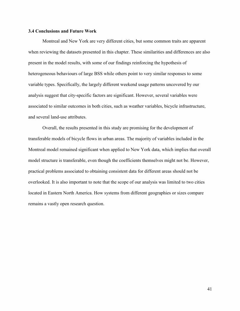
3.4 Conclusions and Future Work ............................................................................................. 41
CHAPTER 4: CONCLUSION ..................................................................................................... 42
5.1 Significant Contributions .................................................................................................... 42
5.2 Future Research ................................................................................................................... 43
REFERENCES ............................................................................................................................. 44
X
List of Tables
Table 1 Estimation Results ........................................................................................................... 20
Table 2 Aggregate Measures of Fit ............................................................................................... 23
Table 3 Descriptive Summary of sample characteristics: Montreal ............................................. 32
Table 4 Descriptive Summary of sample characteristics: New York ........................................... 33
Table 5 Model Estimation Results: Montreal ............................................................................... 39
Table 6 Model Estimation Results: New York ............................................................................. 40
XI
List of Figures
Figure 1 Variation of availability during the day around BIXI stations (estimation sample) ...... 13
Figure 2 Variation of availability during the day around BIXI stations (prediction based on
validation sample) ......................................................................................................................... 25
XII
List of Abbreviations
BIXI Bicycle-Taxi
BSS Bicycle Sharing Systems
CaBi Capital Bikeshare
CBD Central Business District
FQRNT Fonds Québécois de Recherche Nature et Technologie
GHG Green House Gas
GIS Geographic Information System
IT Information Technology
LL Log-Likelihood
LLR Log-Likelihood of Restricted Model
LLUR Log-Likelihood of Unrestricted Model
MAPE Mean Absolute Percent Error
MGOL Mixed Generalized Ordered Logit
ML Maximum Likelihood
NHTS National Household Travel Survey
NSERC National Sciences and Engineering Research Council
PBSC Public Bike System Company
QMC Quasi-Monte Carlo
RMSE Root Mean Square Error
SCD Sub-City District
SVLS Système de Vélos en Libre-Service
1
CHAPTER 1: INTRODUCTION
1.1 Background
The first Bikesharing system (BSS) started operation in Europe in the 1960s, and have
since spread across the globe. According to De Maio (2009) and Shaheen et al. (2010), the
history of bikesharing can be broken down into 4 generations of systems. In the first generation
of BSS, bikes were painted vivid colors and left unlocked around the city so that anyone could
use them. The second generation of BSS required coin deposits in order to unlock a bike. These
early attempts both failed due to user anonymity and a lack of temporal constraints on rentals.
The third generation of BSS was far more successful. These information technology (IT)-based
systems featured user-interface technology or operators at docking stations, required user
identification, and started to implement membership programs and time constraints on usage.
Finally, a fourth generation of systems has emerged in recent years, known as demand-
responsive multimodal systems. Fourth-generation systems feature bicycle redistribution
systems, and attempt to integrate bikesharing with public transit or car-sharing programs. This
thesis will feature studies of two such fourth-generation systems: BIXI in Montreal, and Citi
Bike in New York.
BIXI Montreal kicked-off in May 2009, with a fleet of 3000 bicycles distributed between
300 stations. In August 2009, BIXI Montreal expanded to 411 stations and 5000 bikes. In 2010,
it recorded over 3.4 million trips over the course of the season (PBSC, 2010), which lasts from
mid-April to Mid-November, due to weather constraints. Although the system is widely regarded
as being successful, it has faced significant financial issues since it was put in place. These issues
suggest that a more thorough understanding of bikesharing systems would be beneficial and
2
would help these systems thrive and expand, which in turn would allow urban populations to
decrease their environmental footprint while enjoying health benefits.
New York is the most populous city in the US, and a prominent tourist destination, with
millions of visitors each year. In 2013, cycling mode share was about 1%, whereas it was only
0.5% in 2007 (Kaufman et al., 2015). While 71.7% of trips in the New York metropolitan area
were carried out using private vehicles, bike trips account for 0.4% of total according to NHTS
(2009). When looking a little deeper in the data, it appears that 49.7% of trips are less than two
miles, and within this category the share of private vehicles reduces to 57.1% while the share of
biking rises to 0.7%. This small increase in bike share around dense urban cores offers
substantial benefits as far as public health, well-being, and perhaps transportation-related Green
House Gas (GHG) emissions. Coupled to the fact that 74% of Citi Bike stations are within a half
mile of subway stations, these facts show the potential of BSS to become an important addition
to mobility options for populations located in dense urban areas. New York’s Citi Bike system is
one of the more recent major public bicycle-sharing systems to have been successfully
implemented, and the largest in the United States. The system was launched in May 2013 with
330 stations and over 6000 bicycles in the Northwest of Brooklyn and the lower half of
Manhattan.
Bicycle sharing systems (BSS) have been receiving increasing amounts of attention in
recent years as complementary modes of transportation in urban areas around the world.
Currently, there are over one million public bicycles worldwide, and over 1,100 cities have
installed or are planning a BSS (Meddin and DeMaio, 2015). These systems present many
advantages, including flexibility, ease of access and use, physical activity and health-related
benefits. These systems also address the issue of bicycle theft for users, a common problem for
3
regular cyclists in urban environments (Bachand-Marleau et al., 2012; Van Lierop et al., 2013).
Additionally, BSS offer a potential solution to the “last mile” problem (Cervero et al., 2013;
Shaheen et al., 2010) and are in tune with current generational trends in transportation. Younger
generations are less willing to drive, more concerned about the environment, and more prone to
use public transit and shared transportation alternatives (Dutzik and Baxandall, 2013). Recent
work by Murphy and Usher (2015) suggests BSS can improve driver awareness of cyclists,
which can result in increased safety for all cyclists. Finally, a recent study conducted by
researchers in London, UK, showed that BSS can be beneficial to the public perception of
cycling, and help broaden the demographic of bicycle users (Goodman et al., 2014).
1.2 Literature Review
In recent years, studies have examined several facets of BSS in various cities of Europe
and North America. These studies can be segmented into four broad groups. The first group of
studies employ actual flow data obtained from the system under consideration to investigate the
factors affecting BSS flows. The second group consists of surveys of user behaviours and
perceptions, while the third is concerned with identifying “problematic” stations and optimizing
rebalancing efforts. Finally, the fourth group of studies is concerned with the transferability of
models of BSS demand and bicycle flows. We will provide a brief overview of research studies
along these four dimensions.
Investigating the Factors of BSS Flows
From our review, this group of studies appears to be the most developed. Several studies
set in individual cities have been published over the course of the last decade. For instance,
Krykewycz et al. (2010) investigated a planned system in Philadelphia, Pennsylvania, using a
raster based Geographic Information System (GIS) to identify possible locations for BSS while
4
using data from European cities to forecast expected demand. Wang et al. (2012) investigated
annual station trips in Minneapolis-St.Paul using three ordinary least squares regression models
and four types of variables: presence of businesses and jobs, socio-demographics, built
environment and transportation infrastructure. A common limitation of these studies is the lack
of detailed temporal resolution. Monthly or annual flow estimations fail to capture short term
variation due to shifts in weather, as well as time of day and weekend variation. Recent work by
Hampshire et al. (2013) used aggregated hourly arrival and departure rates to study the influence
of bicycle infrastructure and land use on bicycle flows. Arrivals and departures were aggregated
at the Sub-City District (SCD) level in Barcelona and Seville, Spain. While the study considered
a detailed temporal resolution, an aggregated spatial resolution at the SCD level was a limitation.
Faghih-Imani et al. (2014) modelled station level arrival and departure rates using flow data from
Montreal’s BIXI system while allowing for fine temporal resolution (hour). The authors
developed linear mixed models to quantify the impact of meteorological, temporal and built
environment attributes on bicycle usage while accommodating for station specific unobserved
effects.
User Surveys
This second set of studies relies on survey data to elicit user experience perceptions.
Buck et al. (2013) analyzed the results of a survey conducted in 2007-2008 to establish the
profiles of short-term users and annual members of Capital Bikeshare (CaBi) in Washington,
DC. Fishman et al. (2014) used survey and trip data from Melbourne, Brisbane, Washington
D.C., London, and Minneapolis-St. Paul to investigate the extent to which BSS can help replace
some of the automobile mode share with bicycle share. The study also examined the influence of
rebalancing needs in order to determine the impact of BSS on vehicle-kilometers travelled.
5
Bachand-Marleau et al. (2011) and Bachand-Marleau et al. (2012), examined the results of a
survey conducted in 2010 with BIXI users, and sought to determine what factors affected system
usage and frequency of use. They found that proximity of home to a docking station had the
greatest impact. In the 2012 paper, the authors used the survey results to examine the relationship
between BIXI and public transit usage.
Identifying Problematic Stations
The third group of studies, and one very relevant to BSS operators, focuses on identifying
problematic stations – stations that are full or empty. Nair et al. (2013) examined system
characteristics, utilization patterns, public transit interaction, and flow imbalances between
stations over time for the Vélib’ system in Paris, France. The authors adopted a stochastic
optimization framework to generate redistribution plans for the Vélib’ system. Fricker and Gast
(2014), studied the effect of the randomness of user decisions on the number of problematic
stations. Kloimüllner et al. (2014) developed a dynamic framework to undertake rebalancing in
real time using historical data from Citybike Wien, from Vienna, Austria. These studies provide
opportunities for BSS operators to go further than rely on one of two options: set rebalancing
schedules based on historical patterns, or reactionary rebalancing when stations go beyond
certain thresholds of availability – too high or too low.
Model Transferability
Of the four groups of studies mentioned in this review, the one concerned with model
transferability is probably the most under-developed. Only a handful of publications were
concerned with determining the degree of transferability of models of BSS demand and flow
patterns. Sarkar et al. (2015), applied unsupervised clustering techniques to data from 10 cities
located all around the world, and gained some very interesting insights into how BSS in these
6
different urban areas compare. The main conclusions of this work were that the larger the
system, the greater the spread of station type and behaviour; and systems with fewer than 100
stations were relatively homogeneous. However, this paper relied solely on historical trends in
BSS data, and did not account for other types of variables. This is a rather severe limitation,
since it does not differentiate the impacts of the broad spectrum of variables. Other studies of
interest include the work of Conway (2014), who applied models developed in Washington, D.C.
to data from Minneapolis-St. Paul and the San Francisco Bay Area. The models did not perform
well when applied to these different urban settings. Once again, this model presents several
shortcomings, since it only accounts for a limited array of land-use variables, and does not
account for weather-related or temporal trends. Rixey (2013) used a regression analysis to assess
how bikesharing ridership levels were affected by demographics and built environment around
stations in Washington, Minneapolis-St. Paul, and Denver. While this study did well on the level
of spatial analysis, it was based on regressions on a small sample (n=265). Furthermore, the
dependent variable was the natural log of monthly rentals, meaning short-term considerations
were not captured, most notably weather and time-of-day trends. Finally, the intent of this study
was to develop a regression framework based on data from three cities, and not to compare these
three cities, which resulted in the authors emphasizing different aspects of their research effort.
1.3 Objectives
As is evident from the BSS literature review presented earlier, there are few studies
exploring the transferability of models of BSS flows and usage patterns, and perhaps fewer that
examine availability of bicycles at stations as a direct metric of analysis. Earlier work has
primarily focused on optimization approaches that rely on historical data of BSS usage, or on
modelling arrival and departure flows. While these studies provide useful insights based on
7
analytical approaches, most fail to consider the impact of a host of exogenous variables on
bicycle availability. Ignoring the impact of these variables would reduce the effectiveness of the
prediction platform for new stations or in locations with rapid land use changes. To elaborate, as
these approaches are mainly based on historical patterns, any change in the station structure and
usage patterns due to changes to land-use (or new developments) might be harder to replicate.
The objective of Chapter 2 is to address this research gap by developing a quantitative model of
station level bicycle availability for Montreal’s BIXI system. This behaviorally quantitative
model should accommodate for the influence of temporal, meteorological, bicycle infrastructure,
built environment and land-use attributes on bicycle availability. Furthering current
understanding of the factors affecting bicycle availability will yield insights into the supply-and-
demand mechanisms of bikesharing systems, and allow the operators to better optimize their
rebalancing procedures.
The second objective of this thesis is to contribute to the fledgling literature on BSS
model transferability by comparing two large BSS from Montreal and New York. Specifically,
earlier research into model transferability has not featured detailed econometric models
incorporating the effects of several types of variables. Understanding how weather and temporal
patterns, as well as bicycle infrastructure and general land-use around stations affect BSS
demand in these two different contexts would provide very valuable insights into how to plan
and operate more successful BSS.
1.4 Thesis Structure
The thesis objectives are with the chapters in the dissertation. Chapter 2 focuses on the
Montreal BSS by developing and estimating a quantitative model of bicycle availability. This
model presents detailed temporal and spatial resolutions, and offers significant insight into the
8
main drivers of BSS demand – temporal, meteorological, bicycle infrastructure, land-use and
built environment. Chapter 3 focusses on the potential to transfer models from different spatial
contexts in order to gain insights into existing systems, or optimize the planning of new ones.
Specifically, we apply a detailed arrivals and departures model developed for Montreal by
Faghih-Imani et al. (2014) to New York, and compare the results to determine how these two
systems respond to various categories of variables – temporal, meteorological, bicycle
infrastructure, land-use and built environment. Finally, chapter 4 provides some concluding
remarks and suggests future directions of study.
9
CHAPTER 2: MODELLING BICYCLE AVAILABILITY IN BICYCLE
SHARING SYSTEMS: A CASE STUDY FROM MONTREAL
3.1 Context
The observed bicycle flows (arrivals and departures) in a BSS are in response to
individuals’ need to travel. Hence, observed flows are significantly influenced by land use and
urban form, meteorological and temporal attributes. For example, Faghih-Imani et al. (2014)
observed clear commuting trends i.e. in the morning period bicycles were likely to be picked up
farther from the Central Business District (CBD) and dropped off at stations in the CBD. Such
systematic movements of bicycles in a single direction are likely to create empty stations away
from the CBD and full stations around the CBD. This pattern can lead to lack of access to
bicycles or empty slots for customers, which is a concern for BSS operators because bicycle
availability is at the heart of BSS user-experience. A lack of available bicycles or space to drop
off a bike after usage discourages individuals from using the system. Hence, it is important for
system operators to ensure that bicycle availability (and empty slot availability) is maintained.
For a fixed station capacity, determining the number of bicycles at the station will automatically
determine the number of empty slots. Therefore by examining bicycle availability we also
observe the availability of empty slots.
In order to address flow imbalances, in most systems BSS operators transfer bikes from
full stations to empty stations to ensure bicycle (or slot) accessibility in the system - the process
referred to as rebalancing. In addition to the commuting trend, several spatial and temporal
relationships can result in asymmetry across the system, thus increasing rebalancing needs (Nair
et al., 2013). Moreover, from an environmental perspective, since rebalancing trucks are the only
source of air pollution related to BSS systems, it is important to minimize negative
environmental externalities. Despite the growth of BSS around the world in recent years and the
10
challenges highlighted above, there are very few studies examining the availability of bicycles or
empty slots at a station. To be sure, there have been studies on optimizing rebalancing operations
using historical data from a data mining based approach (Kloimüllner et al., 2014). However,
these approaches do not consider any behavioral relationships between BSS demand and factors
affecting demand such as socio-demographics and land use.
In this chapter, we estimate an ordered regression model – panel mixed generalized
ordered logit model – using data from BIXI-Montreal for the summer of 2012 to accommodate
for exogenous variables and station level unobserved factors. The estimated model is validated
using a hold-out sample of data from the summer of 2013. Finally, to illustrate its applicability,
an availability prediction exercise is undertaken. The model developed can be employed by BSS
operators to arrive at hourly system state predictions and used for rebalancing operations.
3.2 Data Preparation and Modeling Exercise
The data used for this study was collected from BIXI Montreal’s website based on number
of bicycles available at each station on a minute-per-minute basis between April and August 2012,
for 410 BIXI stations throughout the island of Montreal. For the purposes of this study, data for
seven consecutive days for each station were extracted at random from the months of May to
August. April was excluded since all stations do not start operating the same day. The data was
aggregated to an hourly level and augmented with a host of variables, including weather, location,
bicycle infrastructure, land use and built environment, and TAZ level data. The dataset chosen
consists of 68,880 observations (7 days × 24 hours × 410 stations).
3.2.1 Dependent Variable Definition
An important part of the research exercise is to define station level availability. In our
work, we define bicycle availability as the ratio of bicycles docked at a station to station
11
capacity. Hence, availability of 0 would mean the station is completely empty, while availability
of 1 would imply a full station. Further, as BSS operate in continuous time scale, the availability
measure could also be computed in continuous time. However, this would make the analysis
substantially computationally intensive. Hence, in our approach, we average the minute-by-
minute availability across an hour to generate an hourly availability value for each station. Thus,
a single hourly measure that reflects the state of the system in that hour is computed as the
dependent variable in our analysis. The variable has a range from 0 to 1. The bounded nature of
the dependent variable precludes the consideration of linear regression models for analysis. To
facilitate a parsimonious analysis, we consider a discretization of the variable into five
categories: 0-0.2, 0.2-0.4, 0.4-0.6, 0.6-0.8, and 0.8-1.
In the dataset used for this study, stations were completely empty 10.5% of the time, and
completely full 6.6% of the time (0.05 and 0.95 thresholds). It should be noted that computing
availability at an hourly level makes extreme values of 0 and 1 less likely to occur, hence 0.05
and 0.95 are assumed as thresholds to determine completely empty or full stations, respectively.
Furthermore, in 26.3% of cases, stations were less than 20% full, and in 18.3% of cases, they
were over 80% full. So, in total the stations were unusable 17.1% of the time and were close to
unusable 44.6% of the time. These numbers clearly highlight the potential inefficiency in the
BSS system being studied. Finally, the spatial distribution of the inefficiency also varies
substantially across the system.
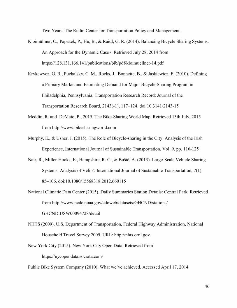
3.2.2 Visual Representation of Availability
In order to better understand bicycle availability and its intimate link with rebalancing
operations, a Geographic Information System (GIS) was used to represent bicycle availability at
all stations in Montreal’s BIXI system, at 8 AM, 12 PM, 5 PM, and 9 PM of a typical summer
12
day (see Figure 1). The availability values plotted represent the weekly mean of availability
values for each time period and station. Figure 1 highlights the typical bicycle movements
throughout the day. At 8 AM, stations located near downtown present low availability levels
(green), whereas stations located further away are more likely to be full (red). At 12 PM, the
trend is reversed. All the morning commutes downtown have filled the downtown stations and
emptied the stations located further out. The 5 PM period has less of a clear distinction, since
downtown stations are closer to empty. Finally, at 9 PM, the downtown stations are nearly
empty, while the stations on the outskirts are full. It is interesting to note that there are many
more balanced stations (yellow) in the morning than in the evening. This is likely due to the
rebalancing efforts of BIXI operators.
13
Figure 1 Variation of availability during the day around BIXI stations (estimation sample)
12 PM 8 AM
9 PM 5 PM
14
3.2.3 Addressing Rebalancing
In using station data compiled from BIXI’s website, it is not possible to differentiate
between user drop-offs and pick-ups versus rebalancing actions. Rebalancing operations
represent an outside attempt to ensure bicycle availability in the system. However, for our
analysis it is critical to account for the presence of artificial flows due to rebalancing. Faghih-
Imani et al. (2014) proposed a heuristic approach to separate rebalancing flows from true flows.
However, the same methodology could not be employed here because rebalancing operations are
likely to have a more prolonged impact on the dependent variable. To elaborate, accounting for
rebalancing on an hourly level would be inadequate, since the number of bikes docked at a
station at a specific time is dependent on how many bikes were there in the previous time frame,
and will affect several subsequent records. In other words, if a rebalancing operation occurs at
2pm, it will not only affect the 2-3pm record. It is much more likely to affect several subsequent
records. In order to address this issue, we created identifier variables to recognize rebalancing
operations and examined their impact over the next 2, 3, 4, 5, 6, and 12 hours. These identifiers
were then provided as input to the models being developed.
3.2.4 Econometric Model Framework
For this study, a Panel Mixed Generalized Ordered Logit (MGOL) model was used to
examine bicycle availability (see Eluru et al. 2008 and Eluru, 2013). Consider that propensity for
station availability is denoted by 𝑦𝑖𝑡∗ where i represents the station (i = 1, 2.. N; N=410 in our
case), t represents the hour under consideration (t = 1,2.. T; T= 168 in our case), and 𝑗 (𝑗 =
1,2, … … … , 𝐽) denotes the station availability levels.
15
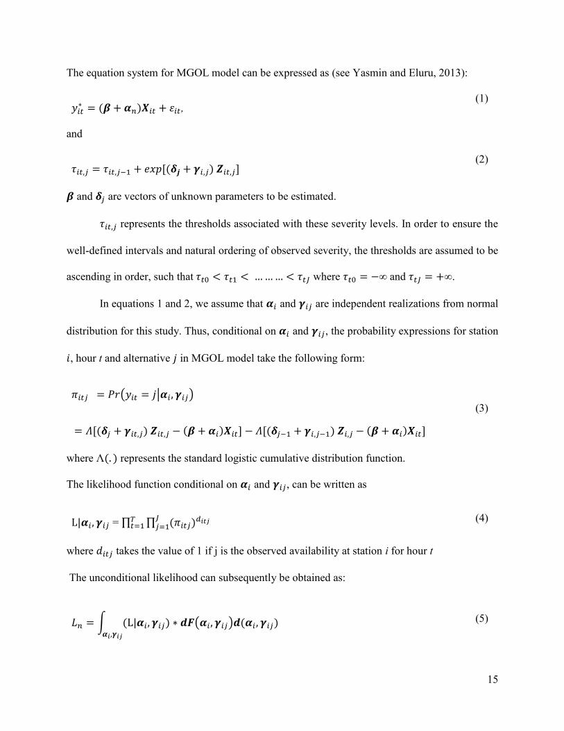
The equation system for MGOL model can be expressed as (see Yasmin and Eluru, 2013):
𝑦𝑖𝑡∗ = (𝜷 + 𝜶𝑛)𝑿𝑖𝑡 + 𝜀𝑖𝑡,
(1)
and
𝜏𝑖𝑡,𝑗 = 𝜏𝑖𝑡,𝑗−1 + 𝑒𝑥𝑝 [(𝜹𝒋 + 𝜸𝑖,𝑗) 𝒁𝑖𝑡,𝑗] (2)
𝜷 and 𝜹𝑗 are vectors of unknown parameters to be estimated.
𝜏𝑖𝑡,𝑗 represents the thresholds associated with these severity levels. In order to ensure the
well-defined intervals and natural ordering of observed severity, the thresholds are assumed to be
ascending in order, such that 𝜏𝑡0 < 𝜏𝑡1 < … … … < 𝜏𝑡𝐽 where 𝜏𝑡0 = −∞ and 𝜏𝑡𝐽 = +∞.
In equations 1 and 2, we assume that 𝜶𝑖 and 𝜸𝑖𝑗 are independent realizations from normal
distribution for this study. Thus, conditional on 𝜶𝑖 and 𝜸𝑖𝑗, the probability expressions for station
𝑖, hour t and alternative 𝑗 in MGOL model take the following form:
𝜋𝑖𝑡𝑗 = 𝑃𝑟(𝑦𝑖𝑡 = 𝑗|𝜶𝑖, 𝜸𝑖𝑗)
= 𝛬[(𝜹𝑗 + 𝜸𝑖𝑡,𝑗) 𝒁𝑖𝑡,𝑗 − (𝜷 + 𝜶𝑖)𝑿𝑖𝑡] − 𝛬[(𝜹𝑗−1 + 𝜸𝑖,𝑗−1) 𝒁𝑖,𝑗 − (𝜷 + 𝜶𝑖)𝑿𝑖𝑡]
(3)
where Λ(. ) represents the standard logistic cumulative distribution function.
The likelihood function conditional on 𝜶𝑖 and 𝜸𝑖𝑗, can be written as
L|𝜶𝑖, 𝜸𝑖𝑗 = ∏ ∏ (𝜋𝑖𝑡𝑗)𝑑𝑖𝑡𝑗𝐽𝑗=1
𝑇𝑡=1 (4)
where 𝑑𝑖𝑡𝑗 takes the value of 1 if j is the observed availability at station i for hour t
The unconditional likelihood can subsequently be obtained as:
𝐿𝑛 = ∫ (L|𝜶𝑖, 𝜸𝑖𝑗) ∗ 𝒅𝑭(𝜶𝑖, 𝜸𝑖𝑗)𝒅(𝜶𝑖, 𝜸𝑖𝑗)𝜶𝑖,𝜸𝑖𝑗
(5)
16
The log-likelihood function is computed as:
ℒ = ∑ 𝐿𝑛
𝑁
𝑖=1
(6)
In this study, we use a Quasi-Monte Carlo (QMC) method proposed by Bhat (2001) to
draw realization from population multivariate distribution. Within the broad framework of QMC
sequences, we specifically use the Halton sequence (250 Halton draws) in the current analysis.
3.3 Estimation Results
The model estimation process started with the estimation of a simple generalized ordered
logit model. Subsequently, the panel mixed generalized ordered logit model was estimated by
building on the results of the simpler models and presented in Table 1. The model estimation
process was guided by statistical significance (at 90% level), parameter interpretability and
parsimony considerations. The results of the exogenous variable impacts are discussed by
variable category.
3.3.1 Constant and Preference Heterogeneity
The constant does not have any substantive interpretation in the model. However, the
presence of statistically significant standard deviation on the constant highlights the presence of
station specific unobserved effects that jointly influence the availability levels for all records for
the station. These joint effects have a standard deviation of 0.3357.
3.3.2 Weather and Temporal
The impact of temperature on latent propensity is negative indicating that with increase
temperature, BIXI availability is likely to reduce. This is expected, as in Montreal, with higher
temperatures BIXI usage is expected to increase. The coefficient for the elevation variable in the
17
propensity is negative and the coefficient in the third threshold is positive, indicating that stations
with a greater elevation are less likely to be full than their counterparts located at lower
elevations. As it is easier to bicycle downhill compared to uphill, stations at an elevation are
more likely to experience asymmetry in travel to and from such stations.
The results for temporal variables follow expected trends. For instance, the AM
coefficient in the propensity function is positive, whereas PM is negative, implying the system is
used more in the afternoon than in the morning. These results are in line with the findings of
Faghih-Imani et al. (2014). It is noteworthy that the coefficients of AM (6-10am) and PM (3-
7pm) are both positive in the second threshold, indicating that stations are more likely to have
low availability than to be balanced during those time frames. Overall, since the AM and PM
periods are when the system is used most, and the flows are most imbalanced, a concentration of
availability around the extremes is expected to occur during those periods. The weekend variable
has a positive coefficient, indicating that the system is used more during the week, probably for
commuting purposes.
3.3.3 Bicycle Infrastructure
The number of BIXI stations in a 250 meter buffer offer interesting results. The presence
of multiple stations in the 250m buffer is likely to reduce the availability at the station of interest,
possibly indicating that these locations are trip generators. On the other hand, in the downtown
region, the impact on availability of neighboring stations is compensated by the interaction term,
thus indicating that availability is marginally influenced by neighboring stations in the downtown
region.
The variable interacted with the downtown variable also affects the second threshold,
with a negative sign indicating that stations located downtown are more likely to be balanced
18
than low. As expected, a refill rebalancing operation increases availability, while a removal
rebalancing operation decreases availability.
3.3.4 Location, Land Use, and Built Environment
The model indicates that stations located in the old port or downtown areas have lower
availability levels overall, which was expected since those are mostly departure areas.
Furthermore, these areas are likely to have higher job concentrations and are conducive to PM
travel - consistent with findings of Faghih-Imani et al. (2014). Street length around the station is
associated to a positive coefficient in the propensity, which is counterintuitive since one would
expect a denser road network in downtown areas. It is important to note that the downtown and
old port dummies interact with this variable. Street length is also associated to a negative
coefficient in the fourth threshold, indicating that areas with high street length values are more
likely to be associated with very high availability.
Walkscore in the vicinity of the station has a negative coefficient indicating highly
walkable neighborhoods are bicycle friendly as well. In addition to the positive mean effect, the
Walkscore variable also has a standard deviation indicating that the impact of walkability varies
across stations. Further, the propensity function indicates that restaurants affect availability based
on time of day. In the AM period presence of restaurants reduces availability while in the PM
period their presence increases availability. This is likely because people usually go to
restaurants more in the late afternoon than in the early morning. Other commercial sites (such as
stores, and libraries) exhibit the opposite effect, with a positive impact on propensity in the AM
period and negative impact on propensity in the PM period. This suggests BIXI users shop more
in the morning than the afternoon. The parameters in the threshold also support the hypotheses
for these variables.
19
3.3.5 TAZ Level Variables
TAZ with large industrial areas are associated with lower availability levels. This result
seems intuitive since industrial parts of town are less likely to be destinations for BIXI users, and
unlikely to be refilled. Further, the variable also has a significant standard deviation indicating
the impact of the variable varies across stations. The positive sign associated to TAZ job density
variable suggests that areas with high job concentrations are mostly drop-off areas. In the second
threshold, TAZ Parks and Recreational Areas are associated to a positive sign, indicating that
stations are more likely to be empty than balanced when they are located in a TAZ with lots of
parks and recreational activities. Finally, in the fourth threshold, TAZ with large commercial
areas are more likely to have stations with high availability than stations with very high
availability. The reasons for this impact are not immediately apparent and warrant further
investigation.
20
Table 1 Estimation Results
Variables Propensity Threshold b/w Low and
Balanced
Threshold b/w
Balanced and High
Threshold b/w High and
Very High
Coef. t-stat Coef. t-stat Coef. t-stat Coef. t-stat
Latent propensity component
Constant -2.5424 -47.74 -0.0728 -11.97 -0.2175 -35.77 0.4049 25.28
Standard Deviation 0.3357 26.42 - - - - - -
Weather, Geography, Temporal
Temperature (ºC) -0.0594 -109.13 - - - - - -
Elevation (*10-1 ; m) -0.0810 -16.91 - - 0.0304 30.61 - -
AM period (6-10 am) 0.1377 5.25 0.1448 7.56 - - - -
PM period (3-7 pm) -0.1106 -4.71 0.1275 7.69 - - - -
Weekend 0.0837 16.05 - - - - - -
Bicycle Infrastructure
Number of BIXI stations in 250m buffer -0.2328 -20.45 - - - - - -
Number of BIXI stations in 250m buffer *Downtown 0.1900 8.10 -0.0450 -19.39 - - - -
Refill (6hr lag) 0.9303 18.48 - - - - - -
Removal (6hr lag) -0.2265 -4.41 - - - - - -
Location, Land use, Built environment
Old port -1.5784 -34.11 - - - - - -
Downtown -1.5639 -15.98 - - - - - -
Street length in 250m buffer (km) 0.3233 24.13 - - - - -0.1328 -29.79
Walkscore (1: low - 7: high ; *10-1) -0.0383 -7.81 - - - - - -
Standard Deviation 0.1463 63.94 - - - - - -
Restaurants in 250m buffer interacted with AM (*10-2) -0.3939 -4.74 - - 0.4687 7.03 - -
Restaurants in 250m buffer interacted with PM (*10-2) 0.6364 9.66 - - - - - -
Commercial venues in 250m interacted with AM (*10-3) 0.5370 3.09 - - -0.7349 -5.95 - -
Commercial venues in 250m interacted with PM (*10-3) -0.4940 -5.04 - - - - - -
TAZ Level
TAZ Industrial and Resources (km2) -3.7085 -19.62 - - - - - -
Standard Deviation 0.4927 2.48 - - - - - -
TAZ Job Density (Jobs per m2) 0.1179 4.47 - - - - - -
TAZ Parks and Recreational Areas (km2) - - 0.1312 4.33 - - - -
Standard Deviation - - 0.3847 6.04 - - - -
TAZ Commerces (km2) - - - - - - 8.9525 54.19
Log-likelihood at convergence -103080 - = Not applicable
Number of observations 68,880
21
3.4 Validation and System-State Prediction
3.4.1 Model Validation
To evaluate the performance of the MGOL model, we undertake a validation exercise on
a hold-out sample. The sample is obtained from 2013 (recall the estimation data is from 2012).
The same data processing approach is employed for the validation sample preparation. The
validation exercise is undertaken at disaggregate and aggregate level. At the disaggregate level,
the predictive log-likelihood of the proposed model is estimated. The predictive log-likelihood is
compared to the log-likelihood at 0 and log-likelihood at sample shares. The model with 32
parameters show substantial improvements relative to the log-likelihood at 0 and log-likelihood
at sample shares. Specifically, the predictive log-likelihood of the MGOL model is -108,117
while the corresponding numbers for log-likelihood at 0 and at sample shares are -110,858 and -
110,088 respectively. The log-likelihood ratio test statistic defined as (2 * LLUR – LLR) is
computed to evaluate the model fit improvement where LLUR corresponds to the log-likelihood
of the unrestricted model (MGOL model) and LLR corresponds to the log-likelihood of the
restricted model (Model at 0 or Model with constants). The log-likelihood ratio test statistic for
our model relative to model at 0 and model with constants are 5,482 and 3,942 respectively. This
improvement in predictive log-likelihood is clearly much larger than the corresponding test
statistic for chi-square distribution at any level of significance. Thus, we clearly see that the
model predicts the station availability levels adequately.
To undertake comparison at an aggregate level, we compare the predicted aggregate
shares with observed aggregate shares. Specifically, we compute the Mean Absolute Percent
Error (MAPE) value and Root Mean Square Error (RMSE) of the predicted shares relative to
observed shares. In addition to the full sample comparison, we also examine model performance
for two spatial categories: (1) Downtown and Old port and (2) > 5kms from Downtown. The
22
results for the comparison are presented in Table 2. Across all three categories, we observe that
the aggregate model performance is very reasonable with MAPE ranging from 12% to 18%. The
RMSE values range from 3.4 to 4.8. Overall, the results indicate high prediction accuracy around
downtown and slightly lower prediction accuracy further from downtown. Even at these further
distances, the errors are quite satisfactory. Further, we observe a slight over prediction in the
extreme alternatives based on our model results.
23
Table 2 Aggregate Measures of Fit
Availability levels/
Measures of fit
Full sample Old port and Downtown >5 km from Downtown (not old port)
Actual shares
(% records)
Predicted shares
(% records)
Actual shares
(% records)
Predicted shares
(% records)
Actual shares
(% records)
Predicted shares
(% records)
0-0.2 25.8 30.7 36.8 43.6 19.5 24.7
0.2-0.4 18.1 16.5 17.3 15.0 17.5 17.3
0.4-0.6 20.4 16.9 16.2 15.0 24.9 18.2
0.6-0.8 17.4 15.6 13.4 11.7 20.6 18.2
0.8-1 18.3 20.3 16.4 14.6 17.6 21.6
MAPE 13.2 12.4 17.8
RMSE 3.4 3.8 4.8
Records 68,880 15,120 16,632
24
3.4.2 System State Prediction
The main strength of the model framework developed is the ability to predict the future
availability levels in the bike sharing system. To illustrate this we provide snapshots of BIXI
system availability at 4 instances of the day. To be sure, the model developed is a probabilistic
model and thus only provides the probability of an availability level. To obtain the actual
availability one has to employ random numbers to arrive at predictions i.e. each random number
realization might alter the prediction for the station state. A system state prediction based on one
set of random numbers is presented in Figure 2. The figure provides evidence of the model’s
applicability for system state prediction.
25
Figure 2 Variation of availability during the day around BIXI stations (prediction based on validation sample)
12 PM 8 AM
9 PM 5 PM
26
3.5 Conclusions and Future Work
Bicycle sharing systems (BSS) have been receiving increasing amounts of attention in
recent years as complementary modes of transportation in urban areas around the world. Earlier
research exploring BSS has mainly focused on arrivals and departures from a station. The current
study addresses this research gap by examining bicycle availability at a station as a direct metric
of analysis. Specifically, we estimate an ordered regression model - panel mixed generalized
ordered logit model - to accommodate for exogenous variables and station level unobserved
factors. Data from Montreal’s BIXI system for the summer of 2012 is employed for model
estimation. The model estimation results are intuitive and along expected lines. Specifically, we
observe that BIXI is used more in the afternoon than in the morning, dense areas tend to be
associated with lower availability levels, and interactions of time of day with land use impact
availability. The estimated model is validated using a hold-out sample of data from the summer
of 2013. The model validation results clearly highlight the predictive capability of the proposed
model. Finally, to illustrate its applicability, we provide system state snapshots for the BIXI
system at 4 instances of the day. Such system state prediction serve as useful inputs for
undertaking rebalancing exercises.
Future work should investigate the level of data aggregation. The original data was
collected on a minute-per-minute basis. This is too fine a resolution for most practical purposes,
but whether the data should be aggregated at a 5 minute, 15 minute, half hour, or as we did
before at the hourly level, is open to debate and should be investigated further. Another aspect of
interest is the influence of spatial spillover effects from neighboring stations in the system.
Finally, the predictive models need to be tied to optimization routines to improve routing
decision for rebalancing trucks.
27
CHAPTER 3: TRANSFERABILITY OF ECONOMETRIC MODELS OF
BICYCLE SHARING DEMAND IN URBAN SETTINGS: A CASE STUDY
OF MONTREAL AND NEW YORK
3.1 Context
Bicycle sharing system usage patterns are influenced by complex interactions between
weather, temporal, bicycle infrastructure, land-use and built environment variables. Toward
enhancing our understanding of the impact of these factors on BSS usage, several statistical
frameworks have been developed. These frameworks are usually complex, requiring substantial
data processing and modeling proficiency at the BSS organization. Not all BSS operators
necessarily have the time, the resources, or the expertise necessary. As a result, BSS planners
often rely on historical trends to plan rebalancing operations. This presents several limitations,
ranging from ignoring the influence of short-term volatile variables such as weather, of isolated
events (festivals etc.), as well as of more long-term variables such as modifications in land-use.
Furthermore, in order to plan successful new systems, reliable prediction frameworks become
even more crucial, since no historical data is available. Given this context, developing models
and frameworks which can be transferred from one urban context to another would be a useful
contribution to the field of BSS planning.
As mentioned in the literature review presented in chapter 1, previous studies of BSS
demand model transferability have shown some promise, but no conclusive evidence of
successful model transfer. Most notably, Conway (2014) emphasized how models developed in
Washington did not perform well when applied to Minneapolis/St. Paul and the San Francisco
Bay Area. Sarkar et al. (2015) found some similarities between different urban contexts, but also
emphasized that the larger the system, the greater the range of station types and the greater the
spread of station behaviour. Quantifying the similarities and differences of BSS in Montreal and
28
New York – two large systems – is in line with these research efforts, and will allow us to shed
more light on these difficult questions.
In 2014, Faghih-Imani et al. presented detailed arrival and departure rates models for
BIXI-Montreal. These models feature detailed spatial and temporal resolutions, and account for
the possibility that flows occurring in successive time frames are more closely correlated than
flows occurring several hours apart. This chapter presents the results obtained when applying
these models to Montreal and New York, and emphasizes the similarities and differences
uncovered. The data used for Montreal is from the same dataset used in chapter 2. Data from
New York was obtained from Citi bike’s website for September 2013, and augmented with
temporal, meteorological, bicycle infrastructure, land-use and built environment variables. The
data from Montreal and New York exhibit similarities related to several attributes (such as
temperature range, length of roads in 250m buffers around stations, number of other stations in
the buffer) while presenting some notable differences (such as more metro stations in New York,
less rain in Montreal, larger average station capacity in New York, less restaurants in station
buffers in Montreal). Section 3.2.1 presents these data in more detail.
3.2 Data and Methodology
3.2.1 Data Preparation and Comparison
Montreal
The data for Montreal was obtained from the same dataset as the one described in chapter
2, so it will not be presented again here in detail. Briefly, trip data was obtained from BIXI-
Montreal’s website for the summer of 2012, and augmented with temporal, meteorological,
bicycle infrastructure, land-use and built environment variables.
29
A few notable differences from the sample formation undertaken in chapter 2 include the
way rebalancing operations were accounted for and the sample size itself. Since rebalancing
operations were not differentiated from user demand in the raw data, spikes in flow rates above
the 99th percentile at the 5-minute aggregation level were considered rebalancing operations, and
the appropriate records were adjusted by setting them equal to the average arrival rates of the two
previous 5-minute records. Data was then further aggregated to an hourly level. Flowrates during
the night time were very low – from 1 AM to 6 AM, so these hours were aggregated into one
record. Two days were sampled at random for each station, resulting in a sample size of 16,400
records (20 hours × 2 days × 410 stations). The sample is distributed evenly across all four
months (22.4 to 26 percent per month), and across all seven days of the week (12.8 to 15.6
percent). The sample might seem small given the range of data available, but there are several
reasons for choosing a moderate sample size: first, run time of linear mixed models can be quite
significant for large samples; second, very large sample size can result in data over-fit and
inflated parameter significance.
New York
Data for New York was obtained from Citi Bike’s website
(https://www.citibikenyc.com/system-data), which provides data for every month of operation
since July 2013. The dataset included the origin and destination stations for each trip, as well as
the start and end time and the user type – member and non-member. The dataset also included
the coordinates of the 330 stations in New York’s BSS. The built environment variables such as
bicycle routes and subway stations were obtained from New York City open data
(https://nycopendata.socrata.com/); the weather information was obtained for Central Park from
the National Climatic Data Center; socio-demographic information was gathered from US 2010
30
census. The sample used for the analysis spanned the month of September 2013. As in the case
of Montreal, two days were sampled at random for each of the 330 stations. This resulted in a
final dataset of 15,840 records (24 hours × 2 days × 330 stations). The sample was well
distributed between weekdays and weekends (28 percent of the records, as expected).
Data Comparison
Since we are using data from two different cities, it is important to examine the two
datasets before presenting the results from the modelling exercise. Data for Montreal can be
found in Table 3, whereas data for New York can be found in Table 4.
As far as weather is concerned, Montreal and New York present similar values for
temperature and relative humidity. However, Montreal is subject to approximately 4 times more
rainy days than New York (9.7 versus 2.6 percent). In the case of temporal variables, data from
Montreal spans April-August 2012, whereas data for New York is from September 2013. The
proportions of weekdays and weekends are similar in both datasets. As for bicycle infrastructure,
stations in New York are slightly bigger than in Montreal (34.4 versus 19.5 bicycle capacity) and
are surrounded by similar numbers of other stations. New York seems to have more bicycle
facilities – as measured by the length of facilities in the 250 meter buffer around the stations –
and similar lengths of streets in the station buffers. It should be noted that since streets in
Montreal are segmented between major and minor roads whereas New York only has one
measure of street length, it is difficult to compare these variables accurately. Finally, land-use
and built environment variables present notable differences. Stations in New York are more than
twice as likely as stations in Montreal to count a metro station in their 250 meter buffer (49.7
versus 21.7 percent). The job and population density variables are on a TAZ basis in Montreal,
which makes it difficult to compare to the open New York data. Similarly, the variables
31
accounting for the number of other commercial enterprises in the buffers also have different
units, making them difficult to compare. New York seems to have a higher density of restaurants.
32
Table 3 Descriptive Summary of sample characteristics: Montreal
Continuous Variables Min Max Mean Std. dev.
Temperature (°C) 5.9 33 20.9 5.2
Relative Humidity (%) 24 99 61.4 16.7
Elevation (m) 14.3 154.8 49.2 24.3
Station Capacity 7 65 19.5 8.0
Number of BIXI Stations in 250m Buffer 1 8 2.2 1.5
Capacity of BIXI Stations in 250m Buffer 7 223 46.9 40.5
Length of Bicycle Facility in 250m Buffer
(km) 0 2.5 0.7 0.51
Length of Minor Roads in 250m Buffer (km) 1.14 6.5 3.6 0.8
Length of Major Roads in 250m Buffer (km) 0 5.7 1.1 1.0
Length of Bus Lines in 250m Buffer (km) 0 12.3 2.8 1.9
TAZ Job density (jobs/m2 * 1000) 0.07 4078.1 141.1 529
Number of Restaurants in 250m Buffer 0 194 24.0 35.3
Number of Other Commercial Enterprises in
250m Buffer 0 1989 121.6 206.9
TAZ Population Density (people/m2 * 1000) 1.01 187.8 59.4 31.6
Area of Parks in 250m Buffer (m2) 0 194907 14551 26962
Walkscore 14 97 62.3 15.7
Categorical Variables Percentage
Rainy Weather 9.7
Weekend 26.5
Friday & Saturday Nights 8.0
Metro Station in 250m Buffer 21.7
Station in Downtown area 17.1
Station in Oldport area 4.9
University in 250m Buffer 17.1
School in 250m Buffer 40.7
33
Table 4 Descriptive Summary of sample characteristics: New York
Continuous Variables Min Max Mean Std. dev.
Hourly Arrivals 0 63 4.4 5.9
Hourly Departures 0 63 4.3 5.8
Temperature (°C) 8.3 34.4 19.4 5.0
Relative Humidity (%) 27 94.2 60.3 15.6
Station Capacity 3 67 34.4 10.8
Number of BIXI Stations in 250m Buffer 1 5 2.2 1.0
Capacity of BIXI Stations in 250m Buffer 10 203 78.3 43.0
Length of Bicycle Facility in 250m Buffer
(km) 0 3.4 1.0 0.6
Street Length in 250m Buffer (km) 1.3 8.4 4.4 1.1
Employment density (jobs/m2 * 1000) 0 432.5 55.8 53.8
Number of Restaurants in 250m Buffer 0 545 54.4 92.2
Density of Other Commercial Enterprises in
250m Buffer (establishments/m2 * 1000) 0 10.1 2.7 1.9
Population Density (people/m2 * 1000) 0.01 67.2 24.9 14.7
Categorical Variables Percentage
Rainy Weather 2.6
Weekend 28.0
Friday & Saturday Nights 7.7
Metro Station in 250m Buffer 49.7
34
3.2.2 Methodology
Since we are using panel data, simple linear regression techniques are not appropriate for
our analysis. Instead, we use a multilevel linear model that explicitly account for flows that
originate at the same station. It should be noted that in the absence of these station-specific
effects – due to repeated observations for each station – the model collapses to a simple linear
regression framework.
The dependent variable under consideration – separate models for arrival and departure
rates normalized by station capacity – is modelled using a linear regression framework which can
be expressed, in its most general form, in the following way:
𝛾𝑞𝑑𝑡 = 𝛽𝑋 + 𝜀
With:
q = 1, 2, 3… : station index
d = 1, 2, 3… : daily index
t = 1, 2, 3… : hourly index
𝛾𝑞𝑑𝑡 is the normalized arrival or departure rate, 𝑋 an L×1 column vector of attributes, 𝛽 the
coefficients (L×1), and 𝜀 the error term – assumed normally distributed across the dataset.
It should be noted the error term can be sub-divided into three unobserved factors: a
station component, a day component, and a time-of-day component. Given the sample size and
number of independent variables considered, it would be too computationally intensive to
estimate the combined influence of all three aspects simultaneously. Hence we consider station
and time-of-day effects to be related. In this structure, each Station-Day combination contains 24
records, resulting in a total of 660 observations. Estimating a full covariance matrix (24 × 24)
would be burdensome, and would be unlikely to yield useful insights. Thus we parameterize the
35
covariance matrix (Ω). In order to estimate a parsimonious specification, we assume a first-order
autoregressive moving average correlation structure with three parameters:
Ω = 𝜎2 (
1 𝜑𝜌 𝜑𝜌2 ⋯ 𝜑𝜌19
𝜑𝜌 1 ⋯ ⋯ ⋯⋮ ⋮ ⋮ ⋮ ⋮
𝜑𝜌19 ⋯ ⋯ ⋯ 1
)
With:
σ = error variance of ε
ϕ = common correlation factor across time periods
ρ = dampening parameter
If the three parameters listed above are significant, they highlight the impact of station specific
effects on the dependent variables.
Model estimation was carried out in SPSS using the Restricted Maximum likelihood
Approach (REML), which differs slightly from Maximum Likelihood (ML) approach, since the
REML estimates the parameters by computing the likelihood function on a transformed dataset.
For additional details concerning model development, the reader is referred to Faghih-Imani et
al. (2014).
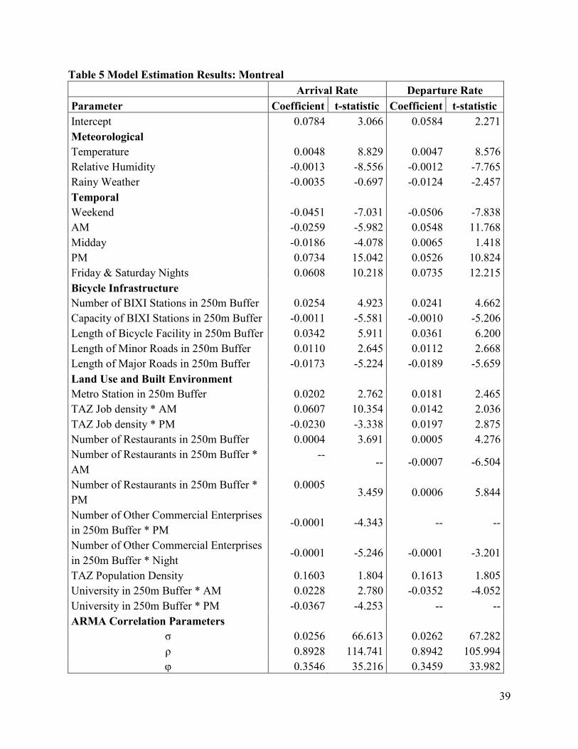
3.3 Results
Full results are available in Tables 5 and 6. The following sections provide brief
commentary on how different categories of variables compare across Montreal and New York
BSS systems.
3.3.1 Model Fit Measures
When examining the Log-Likelihood (LL) values of the models, it appears that for
Montreal, the arrival and departure rate models are performing similarly, with LL values of -
16623.1 and -16102.2, respectively. On the other hand, for New York, the departure rate model
36
far outperformed the arrival rate model, since their LL values were -14826.7 and -17264.1,
respectively. This wide disparity is worth noting and should be investigated further.
3.3.2 Weather
The results for weather variables are consistent across arrival and departure rate models
for Montreal and New York. Higher temperature is associated with higher rates of arrival and
departure, whereas relative humidity and rainy weather are associated with lower utilization
rates. These results make intuitive sense insofar that people tend to prefer biking when the
weather is nice.
3.3.3 Temporal
Temporal variables highlight some interesting differences between BSS use in Montreal
and in New York. Whereas in Montreal the weekend sees a decrease in arrival and departure
rates, this trend is reversed in New York. This suggests that in Montreal the system is used
primarily for commuting purposes during the week, whereas this is not the case in New York.
This could be explained by the fact that New York is a prominent tourist destination, which
could result in increased use by tourists on weekends. This difference in weekend usage patterns
is also picked up by the Friday and Saturday night variable. In Montreal, this coefficient is
positive, signaling increased usage during those time periods. In New York, this variable is not
statistically significant, suggesting that Friday and Saturday evenings do not see a significant
variation in usage pattern when compared to the rest of the week. Finally, the AM, Midday and
PM variables show clear commuting patterns in Montreal, but not in New York.
37
3.3.4 Bicycle Infrastructure
The influence of surrounding stations is similar in both cities, with a high density of
stations associated with increased flows, whereas an increase in the capacity of neighbouring
stations is linked to lower flows. In Montreal, stations witness increased flows when surrounded
by streets with more bicycle lanes, whereas the variable capturing this behaviour is not
statistically significant when applied to New York. This is somewhat surprising since as
mentioned in section 3.2.1 our data suggest there are more bicycle facilities in New York than in
Montreal. However, this lack of significance could be explained by differences in the physical
layout and perceived safety of bicycle lanes in both cities, and deserves future investigation. The
influence of surrounding street length is difficult to assess, since the data for Montreal is
segmented in minor and major roads, whereas New York data only features one variable. For
Montreal, increased length of minor roads is associated to increased utilization of BIXI, whereas
more major roads lead to a decrease in BIXI utilization. For New York, an increase in overall
street length is associated with decreased bicycle flows.
3.3.5 Land-use and Built Environment
Results show several similarities in the influence of land-use around stations on bicycle
arrival and departure rates. Increased population density, number of metro stations and
restaurants in the buffer are all associated with higher utilization of stations. In the case of
restaurants, this is especially true in the evening. In both cities, interacted variables of job density
with AM and PM periods show clear commuting trends for arrival rates – positive in the morning
and negative in the afternoon. However, these trends vanish when looking at departure rates. In
Montreal, job density is associated with higher departure rates both in the AM and the PM. In
New York, these variables are not statistically significant when applied to departure rates. These
38
trends can be explained by the fact that regular users are more likely to use the bikes for morning
and afternoon trips, whereas occasional users are less likely to use the bikes early in the morning,
and their increased presence in the afternoon masks the usage of commuters.
One can also notice some city-specific trends in the data, specifically with respect to the
presence of commercial establishments around stations. In Montreal, surrounding shops are
linked to decreased flows both in the afternoon and the evening. In New York, shops are strongly
linked to increased flows in the afternoon and decreased flows at night.
39
Table 5 Model Estimation Results: Montreal
Arrival Rate Departure Rate
Parameter Coefficient t-statistic Coefficient t-statistic
Intercept 0.0784 3.066 0.0584 2.271
Meteorological
Temperature 0.0048 8.829 0.0047 8.576
Relative Humidity -0.0013 -8.556 -0.0012 -7.765
Rainy Weather -0.0035 -0.697 -0.0124 -2.457
Temporal
Weekend -0.0451 -7.031 -0.0506 -7.838
AM -0.0259 -5.982 0.0548 11.768
Midday -0.0186 -4.078 0.0065 1.418
PM 0.0734 15.042 0.0526 10.824
Friday & Saturday Nights 0.0608 10.218 0.0735 12.215
Bicycle Infrastructure
Number of BIXI Stations in 250m Buffer 0.0254 4.923 0.0241 4.662
Capacity of BIXI Stations in 250m Buffer -0.0011 -5.581 -0.0010 -5.206
Length of Bicycle Facility in 250m Buffer 0.0342 5.911 0.0361 6.200
Length of Minor Roads in 250m Buffer 0.0110 2.645 0.0112 2.668
Length of Major Roads in 250m Buffer -0.0173 -5.224 -0.0189 -5.659
Land Use and Built Environment
Metro Station in 250m Buffer 0.0202 2.762 0.0181 2.465
TAZ Job density * AM 0.0607 10.354 0.0142 2.036
TAZ Job density * PM -0.0230 -3.338 0.0197 2.875
Number of Restaurants in 250m Buffer 0.0004 3.691 0.0005 4.276
Number of Restaurants in 250m Buffer *
AM
-- -- -0.0007 -6.504
Number of Restaurants in 250m Buffer *
PM
0.0005 3.459 0.0006 5.844
Number of Other Commercial Enterprises
in 250m Buffer * PM -0.0001 -4.343 -- --
Number of Other Commercial Enterprises
in 250m Buffer * Night -0.0001 -5.246 -0.0001 -3.201
TAZ Population Density 0.1603 1.804 0.1613 1.805
University in 250m Buffer * AM 0.0228 2.780 -0.0352 -4.052
University in 250m Buffer * PM -0.0367 -4.253 -- --
ARMA Correlation Parameters
σ 0.0256 66.613 0.0262 67.282
ρ 0.8928 114.741 0.8942 105.994
φ 0.3546 35.216 0.3459 33.982
40
Table 6 Model Estimation Results: New York
Arrival Rate Departure Rate
Parameter Coefficient t-statistic Coefficient t-statistic
Intercept 0.0811 2.613 0.0938 3.226
Meteorological
Temperature 0.0028 3.663 0.0021 2.886
Relative Humidity -0.0010 -5.072 -0.0010 -4.991
Rainy Weather -0.0277 -3.587 -0.0378 -4.471
Temporal
Weekend 0.0198 2.065 0.0207 2.332
AM 0.0649 9.330 0.1019 13.921
Midday 0.0773 13.080 0.0817 13.540
PM 0.0986 12.732 0.0789 9.725
Friday & Saturday Nights 0.0134 1.353 0.0052 0.523
Bicycle Infrastructure
Number of BIXI Stations in 250m Buffer 0.0325 3.437 0.0238 2.726
Capacity of BIXI Stations in 250m Buffer -0.0010 -4.457 -0.0008 -3.489
Length of Bicycle Facility in 250m Buffer 0.0004 0.051 -0.0010 -0.138
Street Length in 250m Buffer -0.0117 -2.848 -0.0116 -3.033
Land Use and Built Environment
Metro Station in 250m Buffer 0.0133 3.015 0.0144 3.519
Employment density * AM 0.7390 9.230 0.0446 0.533
Employment density * PM -0.4946 -2.673 -0.0431 -0.222
Number of Restaurants in 250m Buffer 0.0003 6.951 0.0003 7.568
Number of Restaurants in 250m Buffer *
AM 0.0001 1.475
-0.0001 -1.268
Number of Restaurants in 250m Buffer *
PM 0.0003 6.950
0.0002 5.550
Number of Other Commercial Enterprises
in 250m Buffer * PM 13.9214 2.648 15.0814 2.734
Number of Other Commercial Enterprises
in 250m Buffer * Night -2.1323 -1.027 -8.6761 -4.226
Population Density 0.9195 2.999 0.8795 3.099
ARMA Correlation Parameters
σ 0.0405 47.444 0.0390 52.205
ρ 0.8375 160.713 0.8314 143.155
φ 0.7202 115.696 0.6355 85.493
41
3.4 Conclusions and Future Work
Montreal and New York are very different cities, but some common traits are apparent
when reviewing the datasets presented in this chapter. These similarities and differences are also
present in the model results, with some of our findings reinforcing the hypothesis of
heterogeneous behaviours of large BSS while others point to very similar responses to some
variable types. Specifically, the largely different weekend usage patterns uncovered by our
analysis suggest that city-specific factors are significant. However, several variables were
associated to similar outcomes in both cities, such as weather variables, bicycle infrastructure,
and several land-use attributes.
Overall, the results presented in this study are promising for the development of
transferable models of bicycle flows in urban areas. The majority of variables included in the
Montreal model remained significant when applied to New York data, which implies that overall
model structure is transferable, even though the coefficients themselves might not be. However,
practical problems associated to obtaining consistent data for different areas should not be
overlooked. It is also important to note that the scope of our analysis was limited to two cities
located in Eastern North America. How systems from different geographies or sizes compare
remains a vastly open research question.
42
CHAPTER 4: CONCLUSION
5.1 Significant Contributions
Despite the growth of fourth-generation demand-responsive multimodal BSS in recent
years, the literature on these systems is relatively sparse. Most studies of the drivers of BSS
demand and usage patterns do not feature high spatial and temporal resolutions. Furthermore,
very few studies are concerned with bicycle availability at stations, focusing instead on arrival
and departure rates. The first major contribution of this thesis is to develop a detailed panel
mixed generalized ordered logit model of bicycle availability in Montreal’s BIXI system,
featuring detailed temporal and spatial resolutions, and accommodating for exogenous variables
and station level unobserved factors. The estimation results are mostly intuitive, and account for
the influence of several types of variables: temporal, meteorological, bicycle infrastructure, land-
use and built environment. Specifically, our results show that interactions of time of day with
land use impact availability, highlighting clear commuting trends. Overall, the system is used
more in the afternoon than in the morning, and dense areas tend to be associated with lower
availability levels. The validation exercise shows the model performs well, and the system state
predictions provided illustrate how useful this model can be to BSS operators when planning
rebalancing operations.
The second major contribution of this study is to provide a detailed comparison of two
large BSS by applying arrival and departure rate models developed in Montreal to data from
New York. The data show clearly that Montreal and New York are very different cities, even
though some variables present similar ranges. The results from our comparison reinforce the
findings of Sarkar et al. (2015) insofar that they emphasize the heterogeneity of large BSS
systems in terms of temporal patterns. However, our results also show similar outcomes in both
43
cities when it comes to weather variables, bicycle infrastructure, and several land-use attributes.
This suggests that large systems might be more similar than previous research suggested.
5.2 Future Research
The work presented in this thesis opens the way to several future research efforts. First,
the level of data aggregation should be investigated further. The original data for Montreal BIXI
system was collected on a minute-per-minute basis, whereas the New York dataset contained
information about each trip made by users. This level of data resolution is too detailed for most
practical purposes, but whether the data should be aggregated to 5 minute, 15 minute, half hour,
or as we considered at the hourly level, is open to debate. Second, the influence of spatial
spillover effects from neighboring stations in the system needs to be incorporated into the models
employed. This is especially true when analyzing dense networks such as the ones in downtown
Montreal or Manhattan. Third, predictive models need to be tied to optimization routines to
improve routing decision for rebalancing trucks. This opens opportunities for partnerships
between scholars and BSS operators, which could be useful to both parties. Fourth, the degree of
transferability of statistical frameworks developed in or applied to smaller networks and various
geographies should be explored. The scope of our analysis was limited to two large cities located
in Eastern North America. Finally, developing large consistent datasets spanning several cities
and containing meteorological, bicycle infrastructure, land-use and built-environment variables
would be very useful to researchers interested in BSS model transferability.
44
REFERENCES
Bachand-Marleau, J., Larsen, J., & El-Geneidy, A. M. (2011). Much-Anticipated Marriage of
Cycling and Transit: How Will It Work? Transportation Research Record: Journal of the
Transportation Research Board, 2247(-1), 109–117. doi:10.3141/2247-13
Bachand-Marleau, J., Lee, B. H. Y., & El-Geneidy, A. M. (2012). Better Understanding of
Factors Influencing Likelihood of Using Shared Bicycle Systems and Frequency of Use.
Transportation Research Record: Journal of the Transportation Research Board, 2314(-1),
66–71. doi:10.3141/2314-09
Bhat, C.R. (2001). "Quasi-Random Maximum Simulated Likelihood Estimation of the Mixed
Multinomial Logit Model", Transportation Research Part B, Vol. 35, No. 7, pp. 677-693.
Buck, D., Buehler, R., Happ, P., Rawls, B., Chung, P., & Borecki, N. (2013). Are Bikeshare
Users Different from Regular Cyclists?: A First Look at Short-Term Users, Annual
Members, and Area Cyclists in the Washington, D.C., Region. Transportation Research
Record: Journal of the Transportation Research Board, 2387(-1), 112–119.
doi:10.3141/2387-13
Cervero, R., Caldwell, B., & Cuellar, J. (2013). Bike-and-ride: build it and they will come.
Journal of Public Transportation, 16.4, 83-105.
Citi Bike (2015) System data. Retrieved from https://www.citibikenyc.com/system-data
Conway, M. W. (2014). Predicting the Popularity of Bicycle Sharing Stations: An Accessibility-
Based Approach Using Linear Regression and Random Forests. Retrieved from
http://www.indicatrix.org/publications/2014/Conway-Bikeshare-Accessibility.pdf
DeMaio, P. (2009). Bike-sharing: History, Impacts, Models of Provision, and Future. Journal of
Public Transportation. Vol. 12, pp. 41-56.
45
Dutzik, T., and Baxandall, P. (2013). A new direction: Our changing relationship with driving
and the implications for America’s future. U.S. PIRG
Eluru N. (2013). "Evaluating Alternate Discrete Choice Frameworks for Modeling Ordinal
Discrete Variables," Accident Analysis & Prevention, 55 (1), pp. 1-11
Eluru, N., C.R. Bhat, and D.A. Hensher (2008). "A Mixed Generalized Ordered Response Model
for Examining Pedestrian and Bicyclist Injury Severity Level in Traffic Crashes",
Accident Analysis & Prevention, Vol. 40, No.3, pp. 1033-1054
Faghih-Imani A., N. Eluru, A. El-Geneidy, M. Rabbat, and U. Haq, (2014). How does land-use
and urban form impact bicycle flows: Evidence from the bicycle-sharing system (BIXI)
in Montreal, Journal of Transport Geography, Vol. 41, pp. 306-314.
Fishman, E., Washington, S., Haworth, N. (2014). Bike share’s impact on car use: Evidence
from the United States, Great Britain, and Australia, Transportation Research Part D:
Transport and Environment, Volume 31, August 2014, Pages 13-20, ISSN 1361-9209
Fricker, C., & Gast, N. (2014). Incentives and redistribution in homogeneous bike-sharing
systems with stations of finite capacity. EURO Journal on Transportation and Logistics,
1–31. doi:10.1007/s13676-014-0053-5
Goodman, A., Green, J., & Woodcock, J. (2014). The role of bicycle sharing systems in
normalising the image of cycling: An observational study of London cyclists. Journal of
Transport & Health, 1(1), 5–8. http://doi.org/10.1016/j.jth.2013.07.001
Hampshire, R., Lavanya, M., & Eluru, N. (2013). An Empirical Analysis of Bike Sharing Usage
and Rebalancing: Explaining Trip Generation and Attraction from Revealed Preference
Data. Technical Paper, Heinz College, Carnegie Mellon University
Kaufman, S. M., Gordon-Koven, L., Levenson, N. & Moss, M.L. (2015). Citi Bike: The First
46
Two Years. The Rudin Center for Transportation Policy and Management.
Kloimüllner, C., Papazek, P., Hu, B., & Raidl, G. R. (2014). Balancing Bicycle Sharing Systems:
An Approach for the Dynamic Case⋆. Retrieved July 28, 2014 from
https://128.131.166.141/publications/bib/pdf/kloimuellner-14.pdf
Krykewycz, G. R., Puchalsky, C. M., Rocks, J., Bonnette, B., & Jaskiewicz, F. (2010). Defining
a Primary Market and Estimating Demand for Major Bicycle-Sharing Program in
Philadelphia, Pennsylvania. Transportation Research Record: Journal of the
Transportation Research Board, 2143(-1), 117–124. doi:10.3141/2143-15
Meddin, R. and DeMaio, P., 2015. The Bike-Sharing World Map. Retrieved 13th July, 2015
from http://www.bikesharingworld.com
Murphy, E., & Usher, J. (2015). The Role of Bicycle-sharing in the City: Analysis of the Irish
Experience, International Journal of Sustainable Transportation, Vol. 9, pp. 116-125
Nair, R., Miller-Hooks, E., Hampshire, R. C., & Bušić, A. (2013). Large-Scale Vehicle Sharing
Systems: Analysis of Vélib’. International Journal of Sustainable Transportation, 7(1),
85–106. doi:10.1080/15568318.2012.660115
National Climatic Data Center (2015). Daily Summaries Station Details: Central Park. Retrieved
from http://www.ncdc.noaa.gov/cdoweb/datasets/GHCND/stations/
GHCND:USW00094728/detail
NHTS (2009). U.S. Department of Transportation, Federal Highway Administration, National
Household Travel Survey 2009. URL: http://nhts.ornl.gov.
New York City (2015). New York City Open Data. Retrieved from
https://nycopendata.socrata.com/
Public Bike System Company (2010). What we’ve achieved. Accessed April 17, 2014
47
http://www.publicbikesystem.com/what-we-achived/case-studies-info/?id=1
Rixey, R. A. (2013). Station-Level Forecasting of Bikesharing Ridership: Station Network
Effects in Three U.S. Systems. Transportation Research Record: Journal of the
Transportation Research Board, 2387(-1), 46–55. doi:10.3141/2387-06
Sarkar, A., Lathia, N., & Mascolo, C. (2015). Comparing cities’ cycling patterns using online
shared bicycle maps. Transportation, 42(4), 541–559. http://doi.org/10.1007/s11116-015-
9599-9
Shaheen, S. A., Guzman, S., & Zhang, H. (2010). Bikesharing in Europe, the Americas, and
Asia: Past, Present, and Future. Transportation Research Record: Journal of the
Transportation Research Board, 2143(-1), 159–167. doi:10.3141/2143-20
U.S. Census Bureau (2015). U.S. 2010 Census. Retrieved from
http://www.census.gov/2010census/
Van Lierop, D., Grimsrud, M., & El-Geneidy, A. (2013). Breaking into bicycle theft: Insights
from Montreal, Canada. Forthcoming International Journal of Sustainable Transportation
Wang, X., Lindsey, G., Schoner, J., Harrison, A. (2012). Modeling bike share station activity: the
effects of nearby businesses and jobs on trips to and from stations. Paper presented at the
92nd Transportation Research Board Annual Meeting 2012, Washington, DC
Yasmin. S., and N. Eluru (2013), "Evaluating Alternate Discrete Outcome Frameworks for
Modeling Crash Injury Severity," Accident Analysis & Prevention, 59 (1), pp. 506-52