Page 1
Development and Validation of an Electromagnetic
Formation Flight Simulation as a Platform for Control
Algorithm Design
Bruno Alvisio, David W. Miller, Alvar Saenz-Otero
February 2015 SSL # 22-14
Page 3
Development and Validation of an Electromagnetic
Formation Flight Simulation as a Platform for Control
Algorithm Design
Bruno Alvisio, David W. Miller, Alvar Saenz-Otero
February 2015 SSL # 22-14
This work is based on the unaltered text of the thesis by Bruno Alvisio submitted to the
Department of Aeronautics and Astronautics in partial fulfillment of the requirements for
the degree of Master of Science at the Massachusetts Institute of Technology.
1
Page 5
Development and Validation of an Electromagnetic
Formation Flight Simulation as a Platform for Control
Algorithm Design
by
Bruno Alvisio
Submitted to the Department of Aeronautics and Astronauticson December 19, 2014, in partial fulfillment of the
requirements for the degree ofMaster of Science in Aeronautics and Astronautics
Abstract
Electromagnetic Formation Flight (EMFF) consists of using electromagnetic forcesto position or orient satellites in a relative target location or attitude and achieve acertain target formation on orbit. This thesis introduces the fundamental equationsof EMFF and the design of the Resonant Inductive Near-Field Generation System(RINGS). RINGS is a testbed composed of two vehicles that are used to demonstrateEMFF in a 6 DoF environment. In this thesis, a RMS current level controller ismodeled and implemented in RINGS to give the system electromagnetic actuationcapability. Subsequently, a simulation of RINGS that incorporates an EM dynamicsmodel applicable to two RINGS vehicles operating in close proximity is developed.This model was validated using a set of open-loop maneuvers by comparing it withdata obtained from experiments using the RINGS aboard the International Space Sta-tion (ISS). Finally, this simulation was used to test linear controllers that incorporatean ‘Adaptive Control’ approach to achieve system stability for a specific configurationand range of disturbances.
Thesis Supervisor: David W. MillerTitle: Professor of Aeronautics and Astronautics
Thesis Supervisor: Alvar Saenz-OteroTitle: Principal Research Scientist
3
Page 7
Acknowledgments
This work was performed primarily under contract # Z660401 with the Univer-
sity of Maryland as part of the International Space Station SPHERES Integrated
Research Experiments (InSPIRE) and Resonant Inductive Near-Field Generation
System (RINGS) programs from DARPA, administered under NASA contract #
NNH11CC33C. The author gratefully thanks the sponsors for their generous sup-
port that enabled this research.
5
Page 9
Contents
1 Introduction 19
1.1 Motivations for Electromagnetic Formation Flight (EMFF) . . . . . . 19
1.2 Previous Work . . . . . . . . . . . . . . . . . . . . . . . . . . . . . . 21
1.2.1 EMFF Control . . . . . . . . . . . . . . . . . . . . . . . . . . 21
1.2.2 EMFF Testbeds . . . . . . . . . . . . . . . . . . . . . . . . . . 22
1.3 Resonant Inductive Near-Field Generation System (RINGS) . . . . . 22
1.3.1 RINGS Hardware Description . . . . . . . . . . . . . . . . . . 23
1.3.2 RINGS Firmware . . . . . . . . . . . . . . . . . . . . . . . . . 26
1.3.3 EMFF Near-Field Dynamics Model . . . . . . . . . . . . . . . 26
1.4 Thesis Overview . . . . . . . . . . . . . . . . . . . . . . . . . . . . . . 29
2 Modeling and Implementation of a PI Current Controller for RINGS 31
2.1 Introduction . . . . . . . . . . . . . . . . . . . . . . . . . . . . . . . . 31
2.2 Motivation . . . . . . . . . . . . . . . . . . . . . . . . . . . . . . . . . 31
2.3 Proportional-Integrator (PI) Controller . . . . . . . . . . . . . . . . . 33
2.4 ‘Ziegler-Nichols’ Method for Tuning PI Controller Gains . . . . . . . 34
2.5 One-Coil Model . . . . . . . . . . . . . . . . . . . . . . . . . . . . . . 36
2.6 One-Coil PI Current Controller Model . . . . . . . . . . . . . . . . . 38
2.7 Two-Coil PI Current Controller Model . . . . . . . . . . . . . . . . . 40
2.8 Summary . . . . . . . . . . . . . . . . . . . . . . . . . . . . . . . . . 45
3 SPHERES - RINGS Simulation (SRS) 47
3.1 Introduction . . . . . . . . . . . . . . . . . . . . . . . . . . . . . . . . 47
7
Page 10
3.2 Description of SPHERES Simulation . . . . . . . . . . . . . . . . . . 47
3.3 Description and Integration of RINGS Simulation . . . . . . . . . . . 51
3.3.1 RINGS Units Firmware & SPHERES - RINGS Communication 55
3.3.2 RINGS PI Current Controller . . . . . . . . . . . . . . . . . . 56
3.3.3 Features Excluded from the SRS . . . . . . . . . . . . . . . . 58
4 SPHERES - RINGS Simulation (SRS) Validation 61
4.1 SPHERES - RINGS Test Design . . . . . . . . . . . . . . . . . . . . . 61
4.2 Coordinate Frames . . . . . . . . . . . . . . . . . . . . . . . . . . . . 63
4.3 RINGS Physical Parameters Tuning . . . . . . . . . . . . . . . . . . . 63
4.4 RINGS Physical Parameters Validation . . . . . . . . . . . . . . . . . 71
4.5 EM Force Validation . . . . . . . . . . . . . . . . . . . . . . . . . . . 76
4.6 RINGS Hardware/Software Verification . . . . . . . . . . . . . . . . . 84
4.7 EM Force Validation: Repulsion . . . . . . . . . . . . . . . . . . . . . 89
4.8 EM Torque Validation . . . . . . . . . . . . . . . . . . . . . . . . . . 91
4.9 Summary . . . . . . . . . . . . . . . . . . . . . . . . . . . . . . . . . 94
5 Evaluation of Closed-Loop Position Controllers Using the SRS 97
5.1 Introduction . . . . . . . . . . . . . . . . . . . . . . . . . . . . . . . . 97
5.2 Description of the CLPC . . . . . . . . . . . . . . . . . . . . . . . . . 98
5.3 Axial Station Keeping Tests for Optimal RU Orientation . . . . . . . 100
5.4 Step Input Tests . . . . . . . . . . . . . . . . . . . . . . . . . . . . . 104
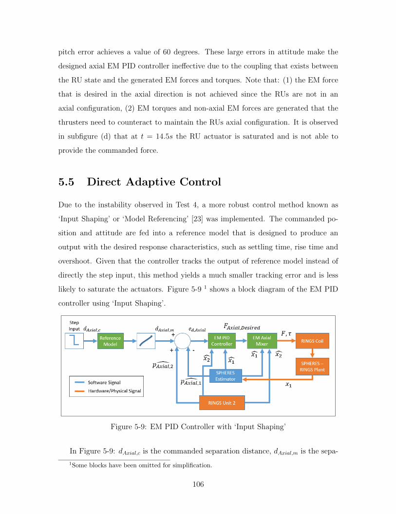
5.5 Direct Adaptive Control . . . . . . . . . . . . . . . . . . . . . . . . . 106
5.6 Summary . . . . . . . . . . . . . . . . . . . . . . . . . . . . . . . . . 107
6 Conclusions and Future Work 109
6.1 Conclusions . . . . . . . . . . . . . . . . . . . . . . . . . . . . . . . . 109
6.2 Future Work . . . . . . . . . . . . . . . . . . . . . . . . . . . . . . . . 110
A RINGS - SPHERES Communication Interface and API 117
A.1 RINGS Communication Interface . . . . . . . . . . . . . . . . . . . . 117
A.1.1 Integration of RINGS to a SPHERES GSP Project . . . . . . 117
8
Page 11
A.1.2 RINGS Packet Structure . . . . . . . . . . . . . . . . . . . . . 118
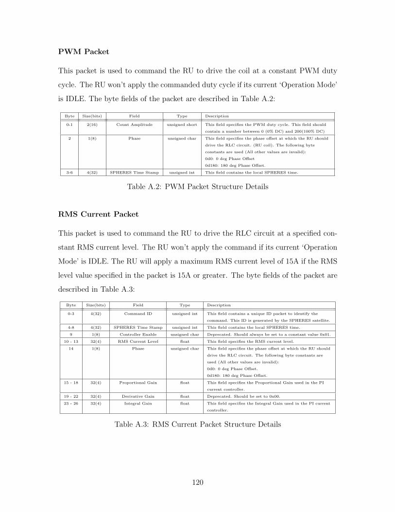
A.1.3 Transmitted Messages . . . . . . . . . . . . . . . . . . . . . . 119
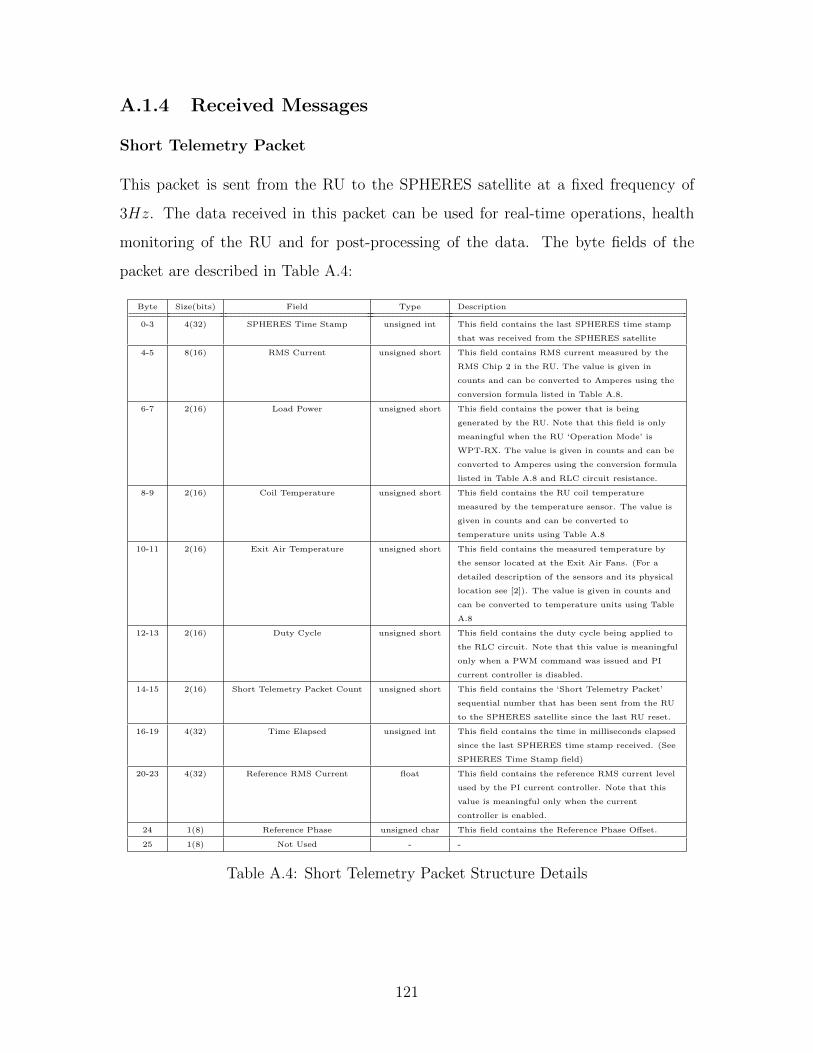
A.1.4 Received Messages . . . . . . . . . . . . . . . . . . . . . . . . 121
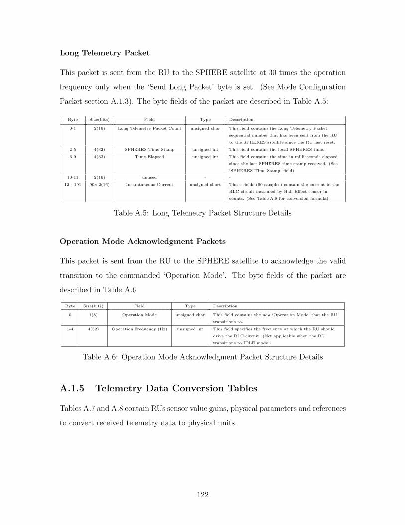
A.1.5 Telemetry Data Conversion Tables . . . . . . . . . . . . . . . 122
A.2 SPHERES - RINGS API . . . . . . . . . . . . . . . . . . . . . . . . . 123
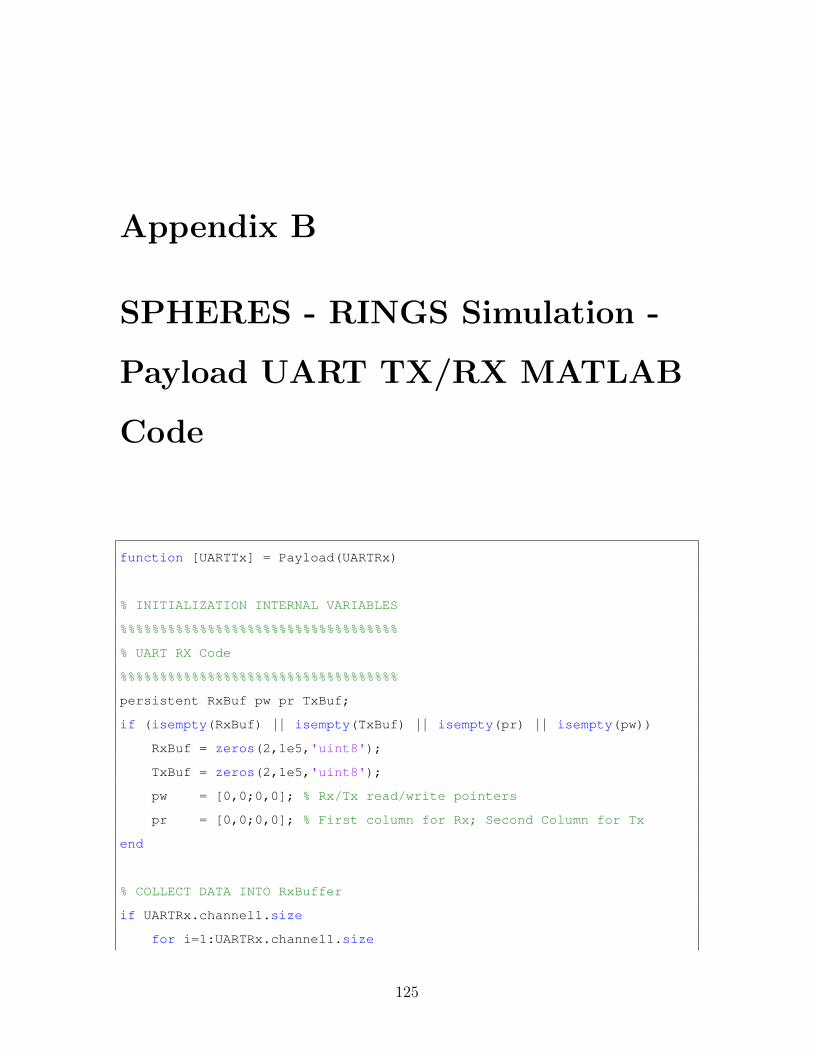
B SPHERES - RINGS Simulation - Payload UART TX/RX MATLAB
Code 125
9
Page 13
List of Figures
1-1 SPHERES-RINGS Unit [1] . . . . . . . . . . . . . . . . . . . . . . . . 23
1-2 RINGS Unit Coil Schematic [2] . . . . . . . . . . . . . . . . . . . . . 24
1-3 RLC Circuit Diagram [2] . . . . . . . . . . . . . . . . . . . . . . . . . 25
1-4 Two Loops of Current [3] . . . . . . . . . . . . . . . . . . . . . . . . . 28
1-5 Near vs Far-Field - Relative Error for Axial Force and Shear Torque [4] 29
2-1 Iss vs. Duty Cycle for different (VBatt) [2] . . . . . . . . . . . . . . . . 32
2-2 RINGS Response to 20 % DC Input Step . . . . . . . . . . . . . . . . 34
2-3 RINGS Response to 60 % DC Input Step . . . . . . . . . . . . . . . . 35
2-4 ‘One-Coil Model’ Block Diagram [2] . . . . . . . . . . . . . . . . . . . 36
2-5 One-coil Model vs. Experiment - Response to 20 % DC Step . . . . . 37
2-6 One-coil Model vs. Experiment - Response to 60 % DC Step . . . . . 37
2-7 PI Current Controller Model Block Diagram . . . . . . . . . . . . . . 38
2-8 One-Coil PI Current Controller Model - System Response to a 12A
Step Input . . . . . . . . . . . . . . . . . . . . . . . . . . . . . . . . . 39
2-9 One-Coil PI Current Controller Model - System Response to a -9A
Input Step . . . . . . . . . . . . . . . . . . . . . . . . . . . . . . . . . 40
2-10 Two-Coil PI Current Controller - Simulation Block Diagram [2] . . . 41
2-11 Coupling coefficient (κ) vs. Axial Separation Distance [2] . . . . . . . 42
2-12 Two-Coil Experimental Set-Up . . . . . . . . . . . . . . . . . . . . . 43
2-13 Two-Coil PI Current Controller Simulation vs. Experiment - Scenario 1 43
2-14 Two-Coil PI Current Controller Simulation vs. Experiment - Scenario 2 44
2-15 Two-Coil PI Current Controller Simulation vs. Experiment - Scenario 3 44
11
Page 14
3-1 SPHERES Test Development Process . . . . . . . . . . . . . . . . . . 48
3-2 SPHERES Simulation Block Diagram [5] . . . . . . . . . . . . . . . . 49
3-3 SRS Block Diagram . . . . . . . . . . . . . . . . . . . . . . . . . . . . 52
3-4 SRS Block Diagram - RINGS Units & EM Physics Model . . . . . . . 53
3-5 SRS Block Diagram - State Input . . . . . . . . . . . . . . . . . . . . 54
3-6 SRS Block Diagram - Output Variables . . . . . . . . . . . . . . . . . 54
3-7 RINGS Communication Buffer . . . . . . . . . . . . . . . . . . . . . . 56
3-8 RLC Circuit Current with Lowpass Filter . . . . . . . . . . . . . . . . 57
3-9 RU RLC Circuit Dynamics Test - Experiment vs. SRS . . . . . . . . 58
4-1 RINGS Test Initial Position Set-Up . . . . . . . . . . . . . . . . . . . 62
4-2 Body (blue) & Inertial (black) Reference Frames . . . . . . . . . . . . 63
4-3 Thruster Test Timeline . . . . . . . . . . . . . . . . . . . . . . . . . . 64
4-4 RINGS Unit Angular Velocity - SRS Results . . . . . . . . . . . . . . 66
4-5 RINGS Unit Angular Velocity - ISS . . . . . . . . . . . . . . . . . . . 67
4-6 SPHERES-RINGS Thrusters Impingement . . . . . . . . . . . . . . . 68
4-7 Gyro Readings - ISS vs. SRS . . . . . . . . . . . . . . . . . . . . . . 70
4-8 Y-Axis Accelerometer Readings - ISS vs. SRS . . . . . . . . . . . . . 70
4-9 RU 1 Position - ISS Test vs. SRS . . . . . . . . . . . . . . . . . . . . 73
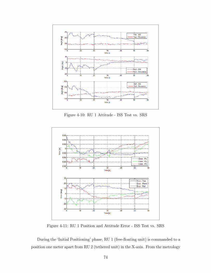
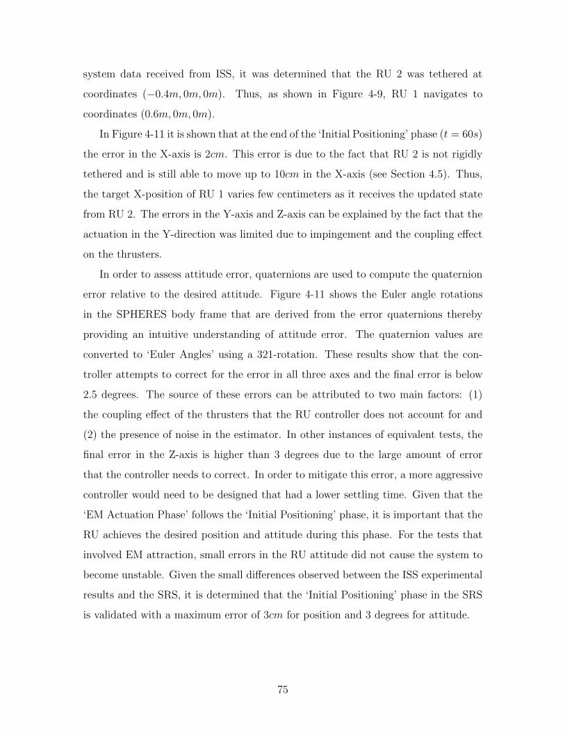
4-10 RU 1 Attitude - ISS Test vs. SRS . . . . . . . . . . . . . . . . . . . . 74
4-11 RU 1 Position and Attitude Error - ISS Test vs. SRS . . . . . . . . . 74
4-12 EM Actuation Test - Current Profile . . . . . . . . . . . . . . . . . . 76
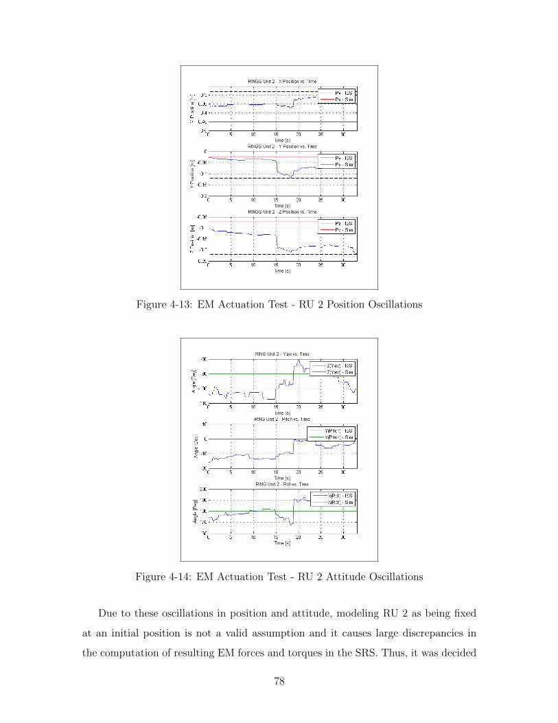
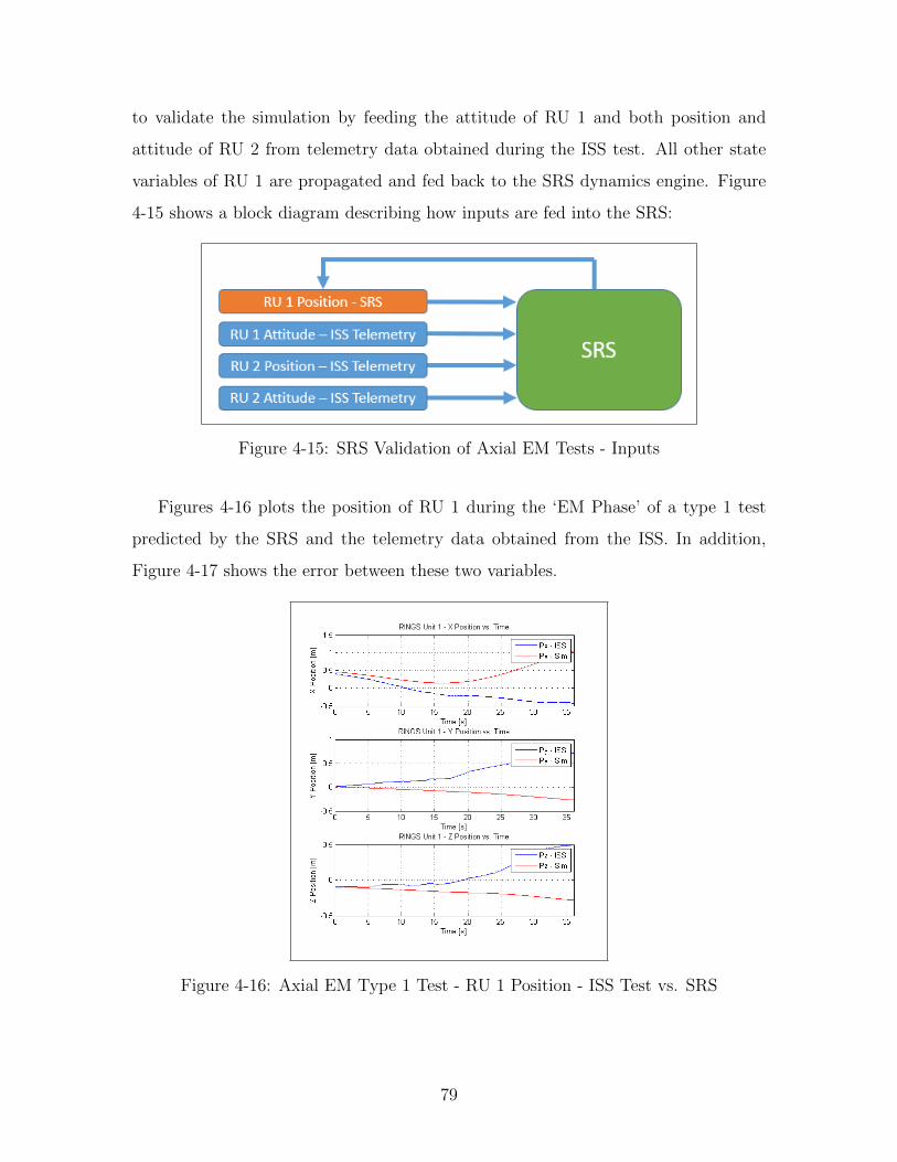
4-13 EM Actuation Test - RU 2 Position Oscillations . . . . . . . . . . . . 78
4-14 EM Actuation Test - RU 2 Attitude Oscillations . . . . . . . . . . . . 78
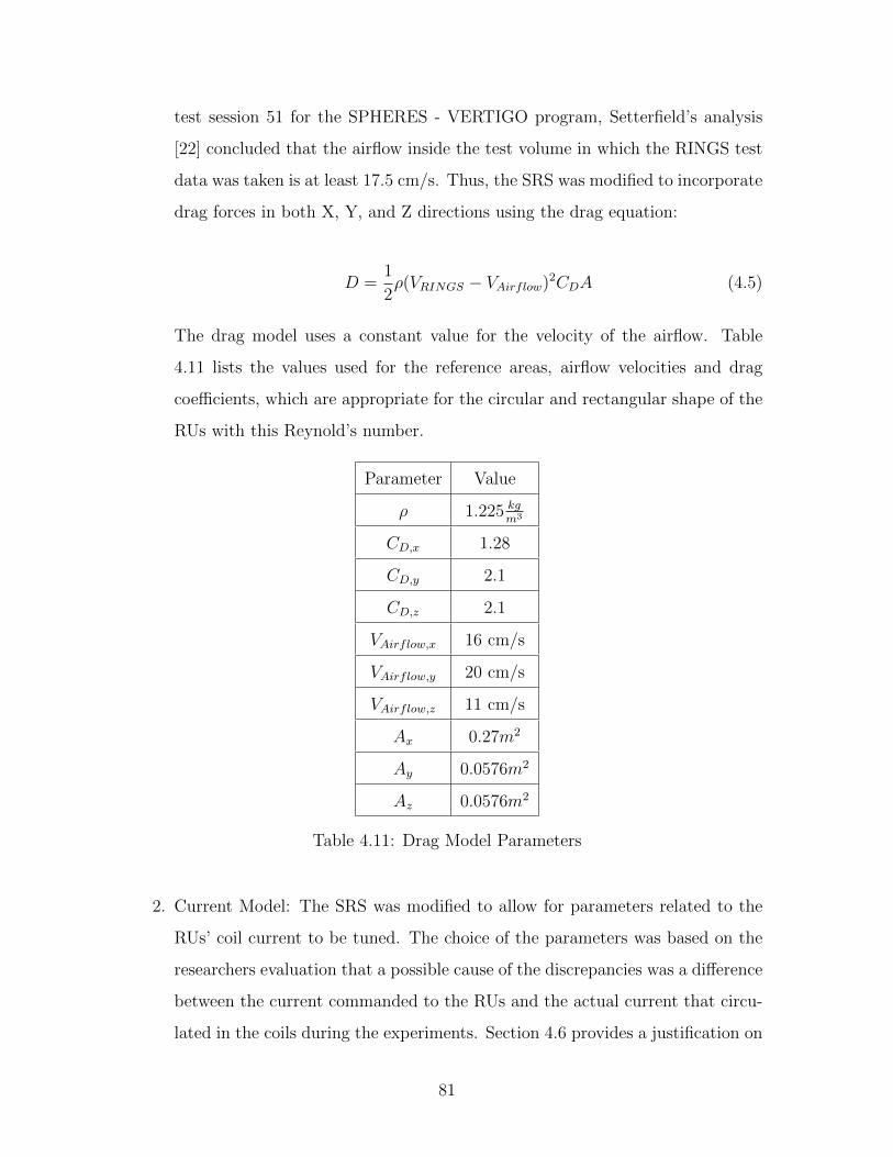
4-15 SRS Validation of Axial EM Tests - Inputs . . . . . . . . . . . . . . . 79
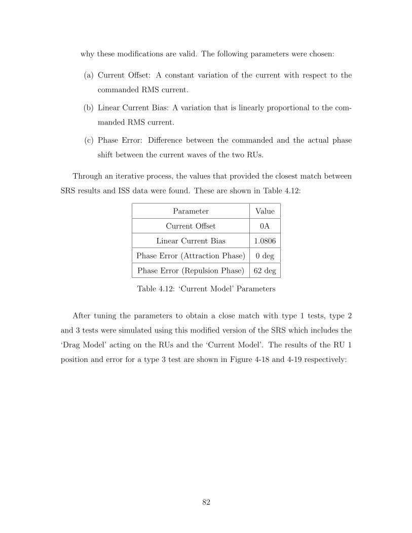
4-16 Axial EM Type 1 Test - RU 1 Position - ISS Test vs. SRS . . . . . . 79
4-17 Axial EM Type 1 Test - RU 1 Position Error - ISS Test vs. SRS . . . 80
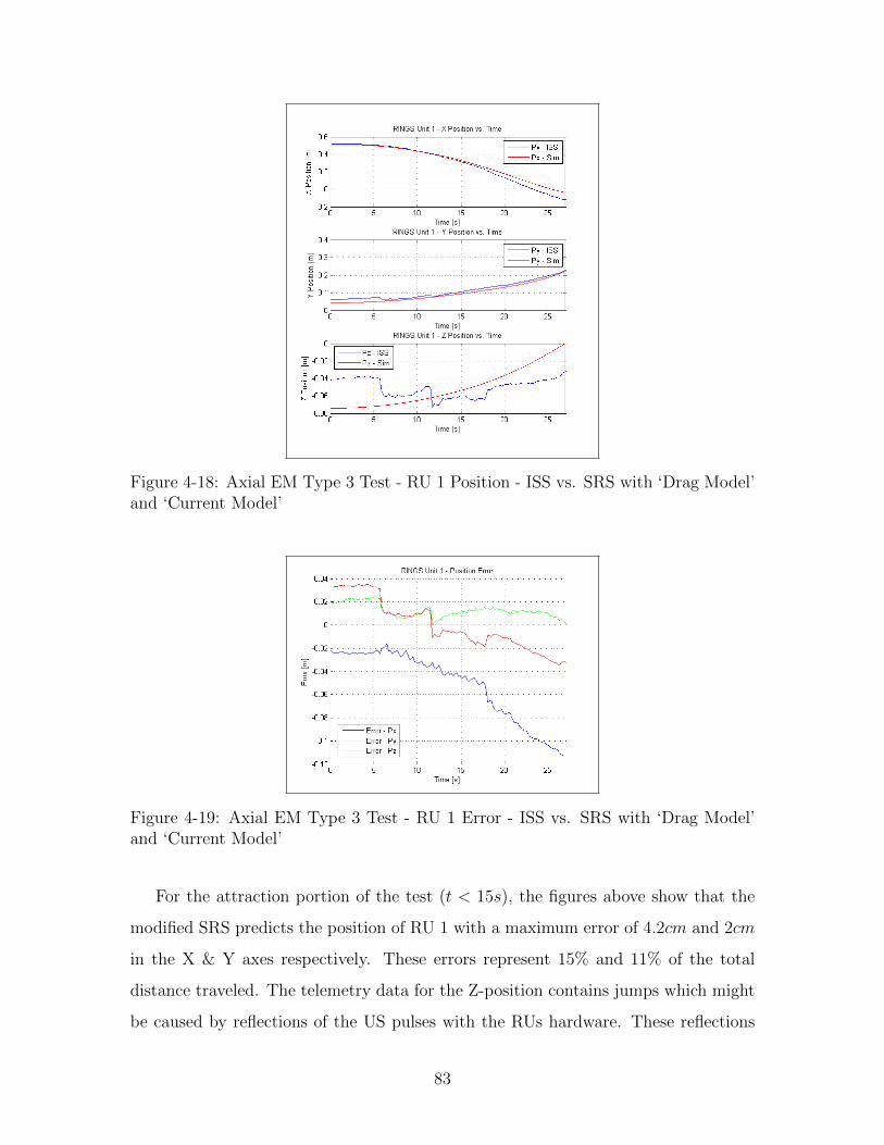
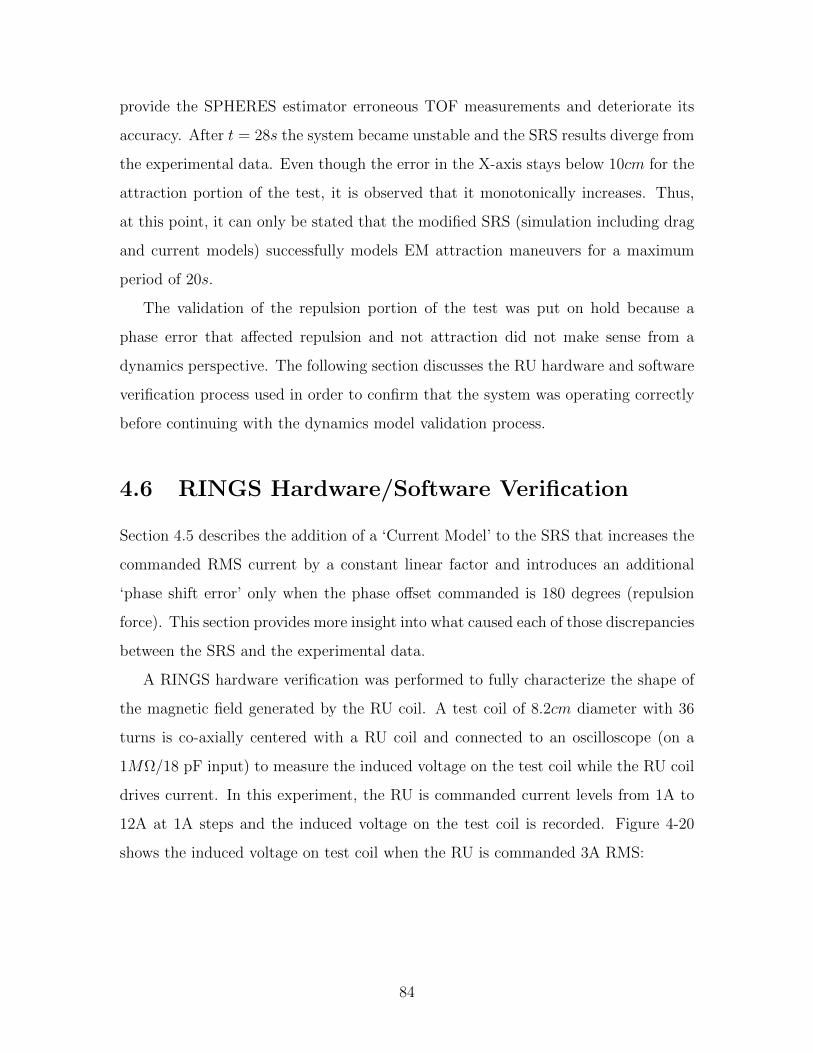
4-18 Axial EM Type 3 Test - RU 1 Position - ISS vs. SRS with ‘Drag Model’
and ‘Current Model’ . . . . . . . . . . . . . . . . . . . . . . . . . . . 83
12
Page 15
4-19 Axial EM Type 3 Test - RU 1 Error - ISS vs. SRS with ‘Drag Model’
and ‘Current Model’ . . . . . . . . . . . . . . . . . . . . . . . . . . . 83
4-20 RINGS Hardware Verification - Induced Voltage - 3A RMS . . . . . . 85
4-21 RINGS Hardware Verification - FFT - 3A RMS . . . . . . . . . . . . 85
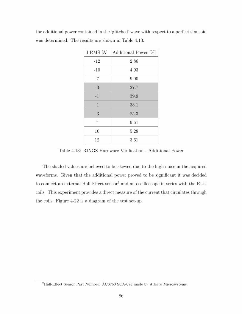
4-22 Hardware Verification Test Setup . . . . . . . . . . . . . . . . . . . . 87
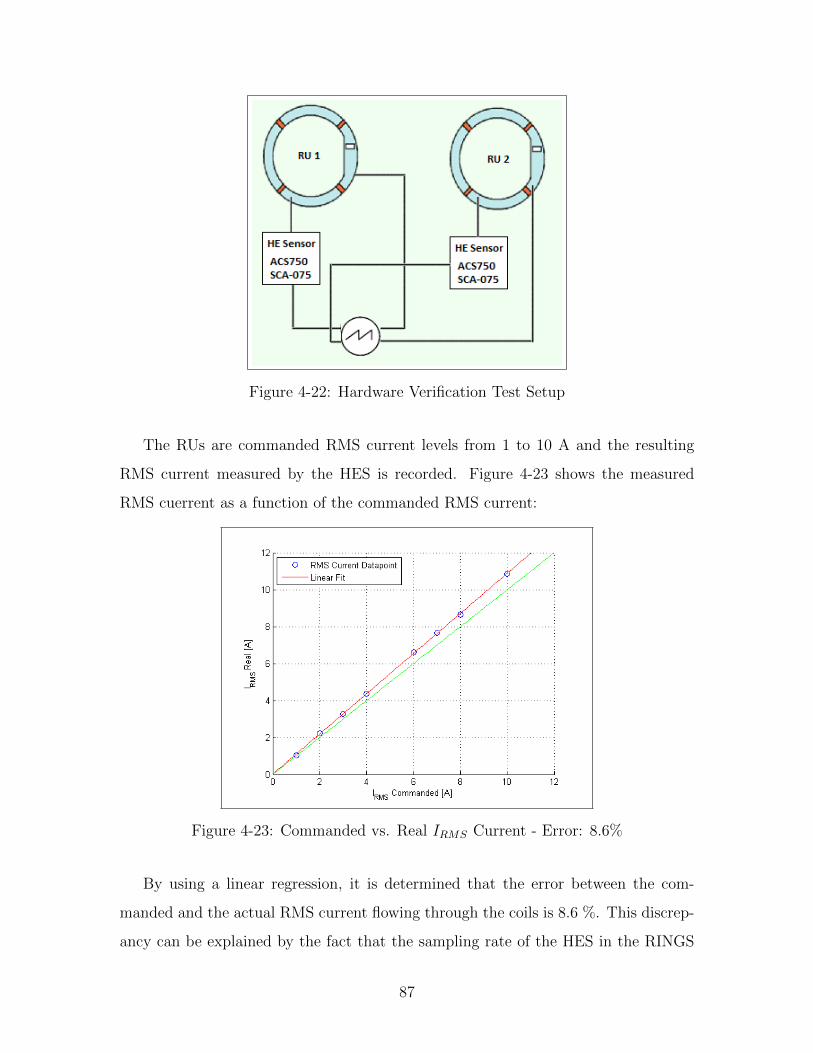
4-23 Commanded vs. Real IRMS Current - Error: 8.6% . . . . . . . . . . . 87
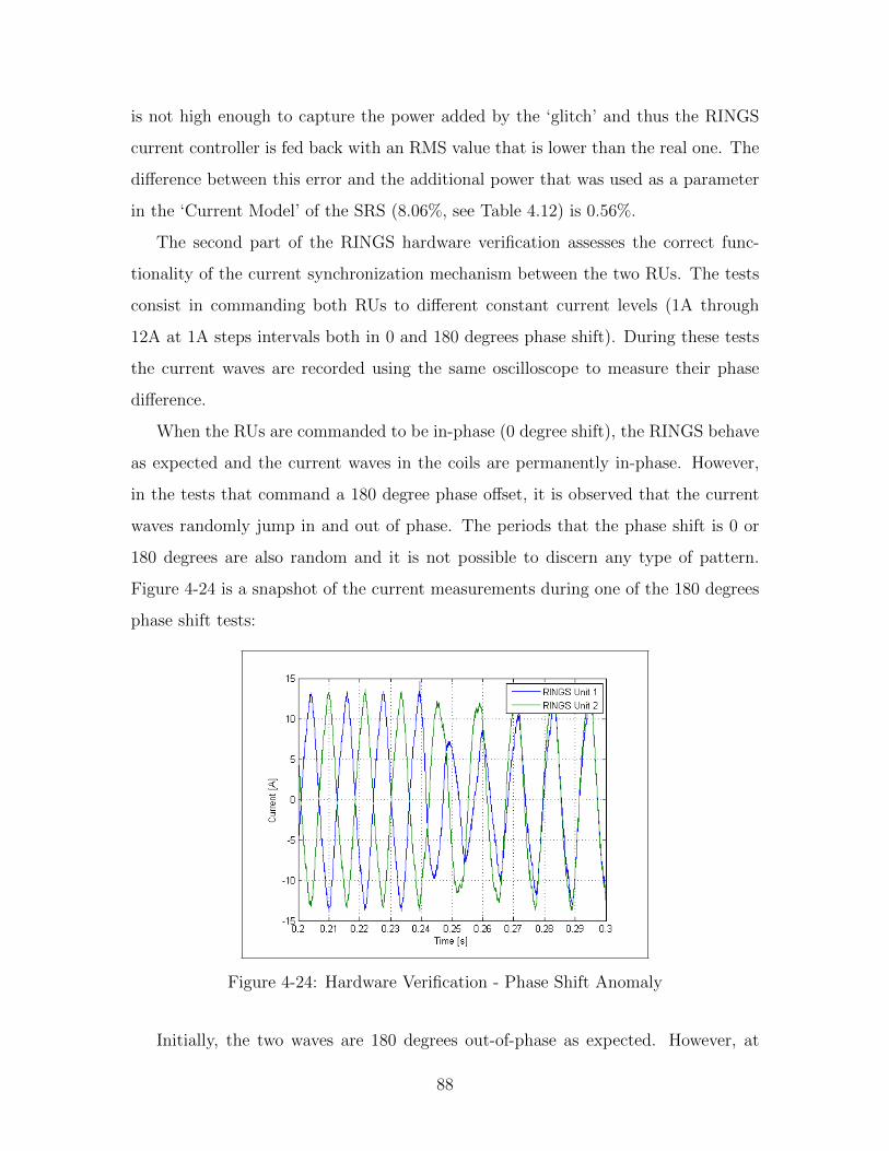
4-24 Hardware Verification - Phase Shift Anomaly . . . . . . . . . . . . . . 88
4-25 Axial EM Repulsion Test - Position . . . . . . . . . . . . . . . . . . . 90
4-26 Axial EM Repulsion Test - Error . . . . . . . . . . . . . . . . . . . . 90
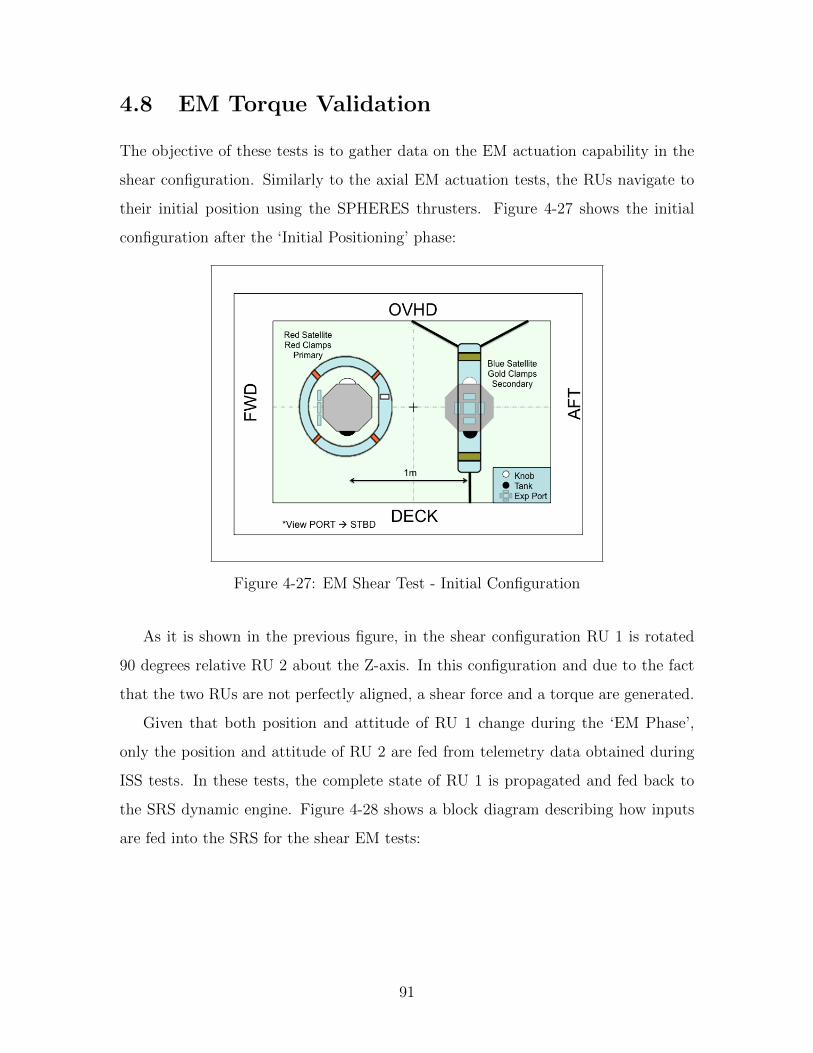
4-27 EM Shear Test - Initial Configuration . . . . . . . . . . . . . . . . . . 91
4-28 SRS Validation of Shear Tests - Inputs . . . . . . . . . . . . . . . . . 92
4-29 Shear EM Test Type 1 - RU 1 Position - ISS vs. SRS . . . . . . . . . 92
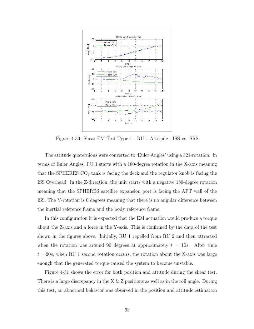
4-30 Shear EM Test Type 1 - RU 1 Attitude - ISS vs. SRS . . . . . . . . . 93
4-31 Shear EM Test Type 1 - RU 1 Error - Validation . . . . . . . . . . . 94
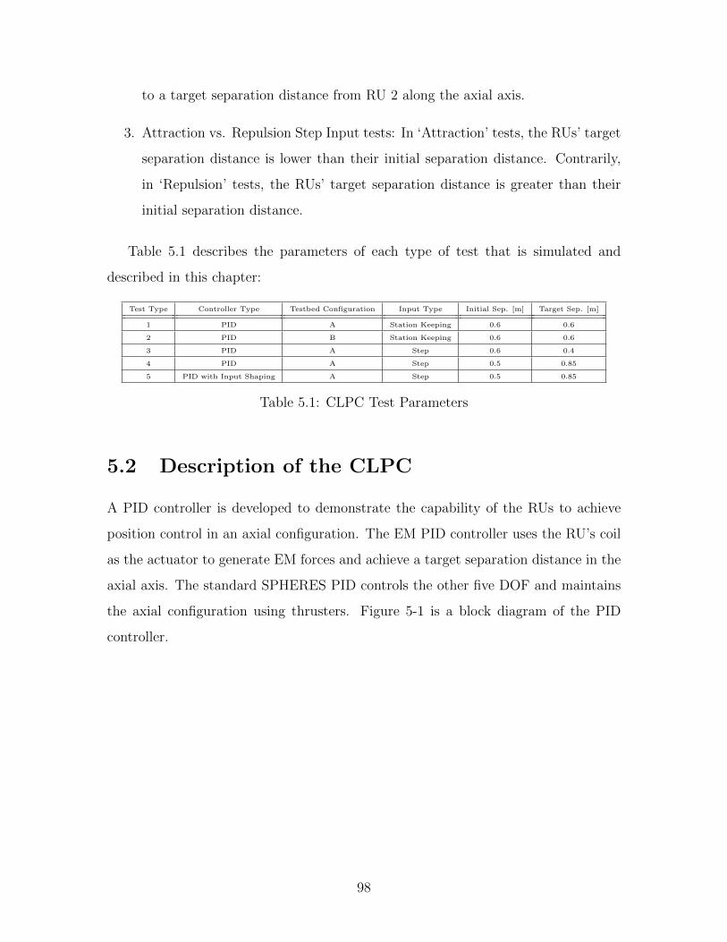
5-1 PID Position Controller . . . . . . . . . . . . . . . . . . . . . . . . . 99
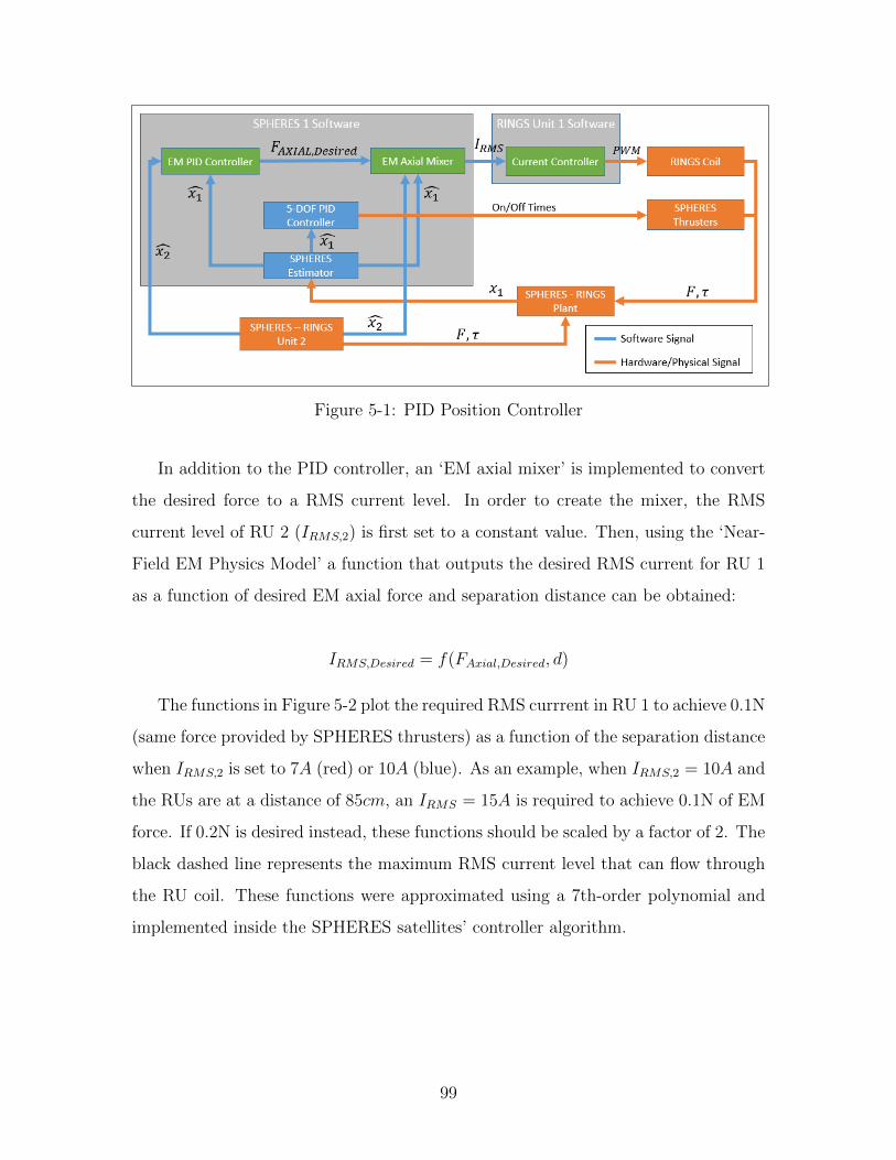
5-2 Mixer Function for Axial Configuration - IRMS/F vs. Axial Separation
Distance . . . . . . . . . . . . . . . . . . . . . . . . . . . . . . . . . . 100
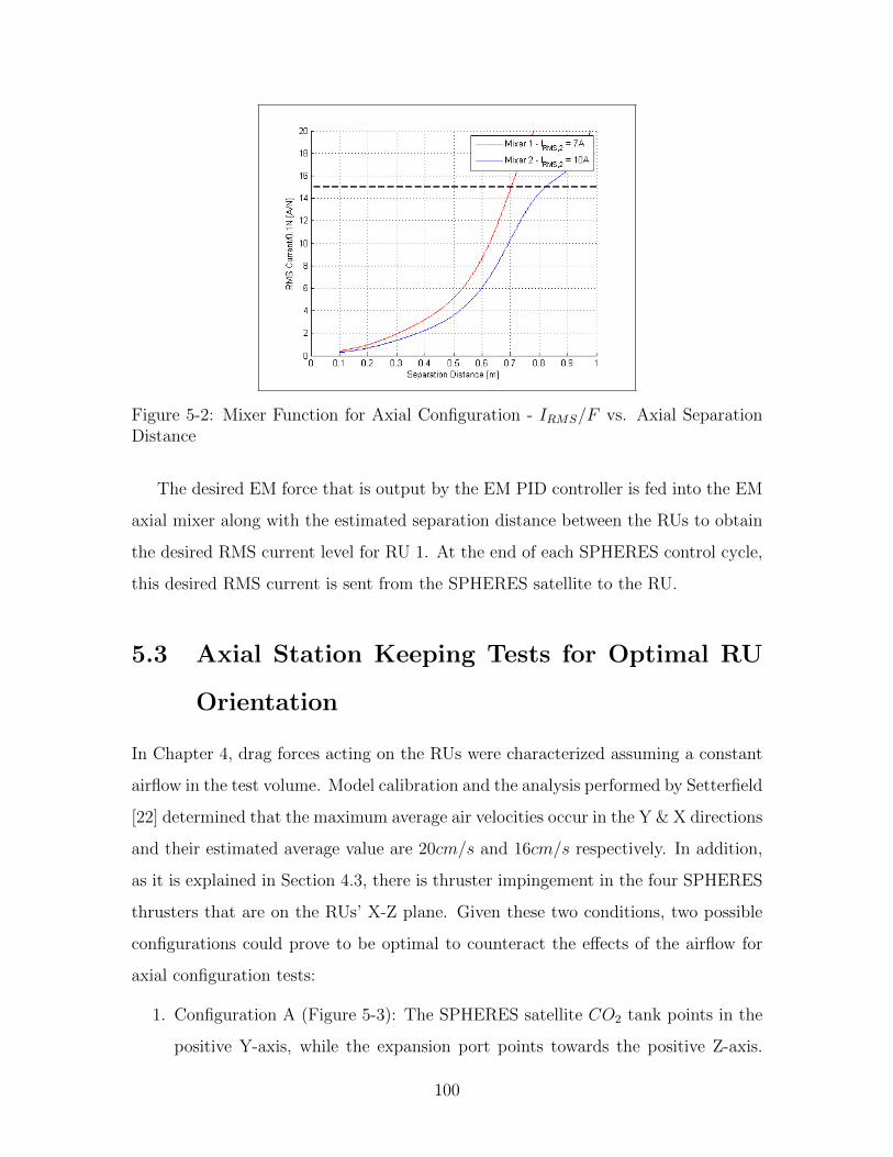
5-3 Test - Configuration A . . . . . . . . . . . . . . . . . . . . . . . . . . 101
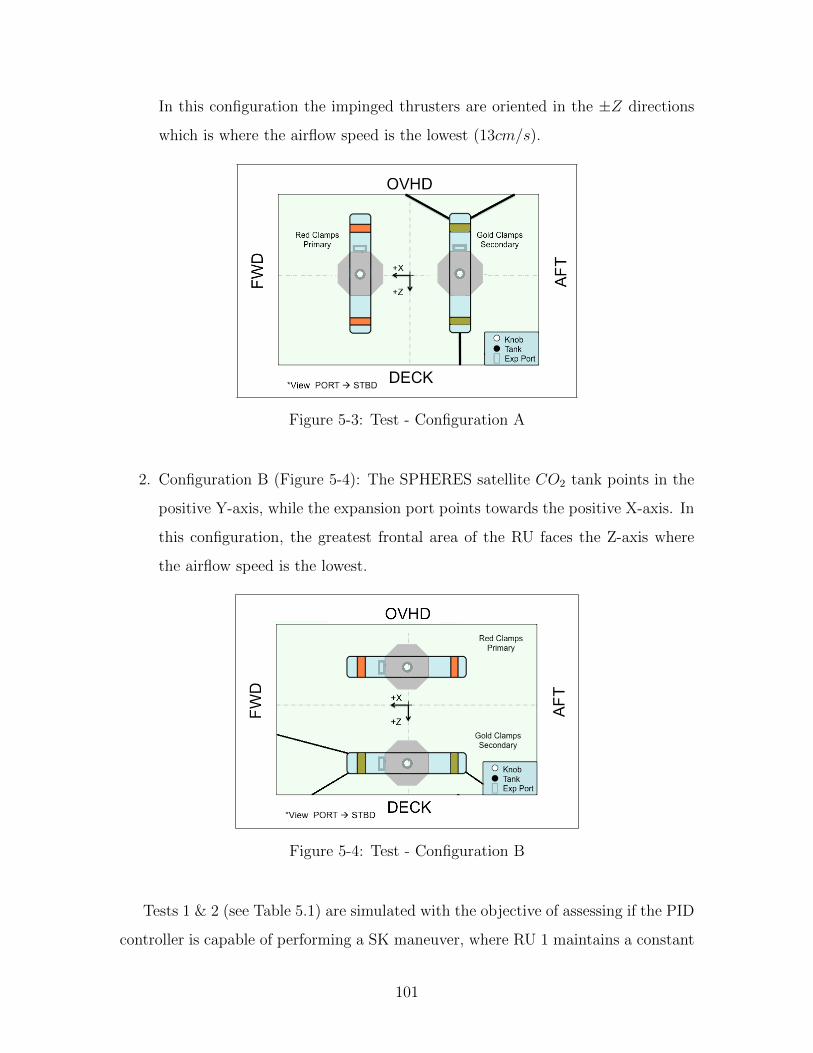
5-4 Test - Configuration B . . . . . . . . . . . . . . . . . . . . . . . . . . 101
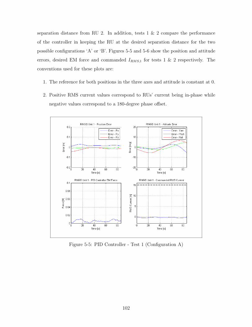
5-5 PID Controller - Test 1 (Configuration A) . . . . . . . . . . . . . . . 102
5-6 PID Controller - Test 2 (Configuration B) . . . . . . . . . . . . . . . 103
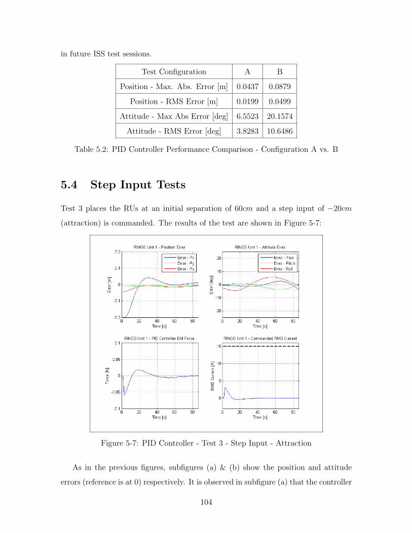
5-7 PID Controller - Test 3 - Step Input - Attraction . . . . . . . . . . . 104
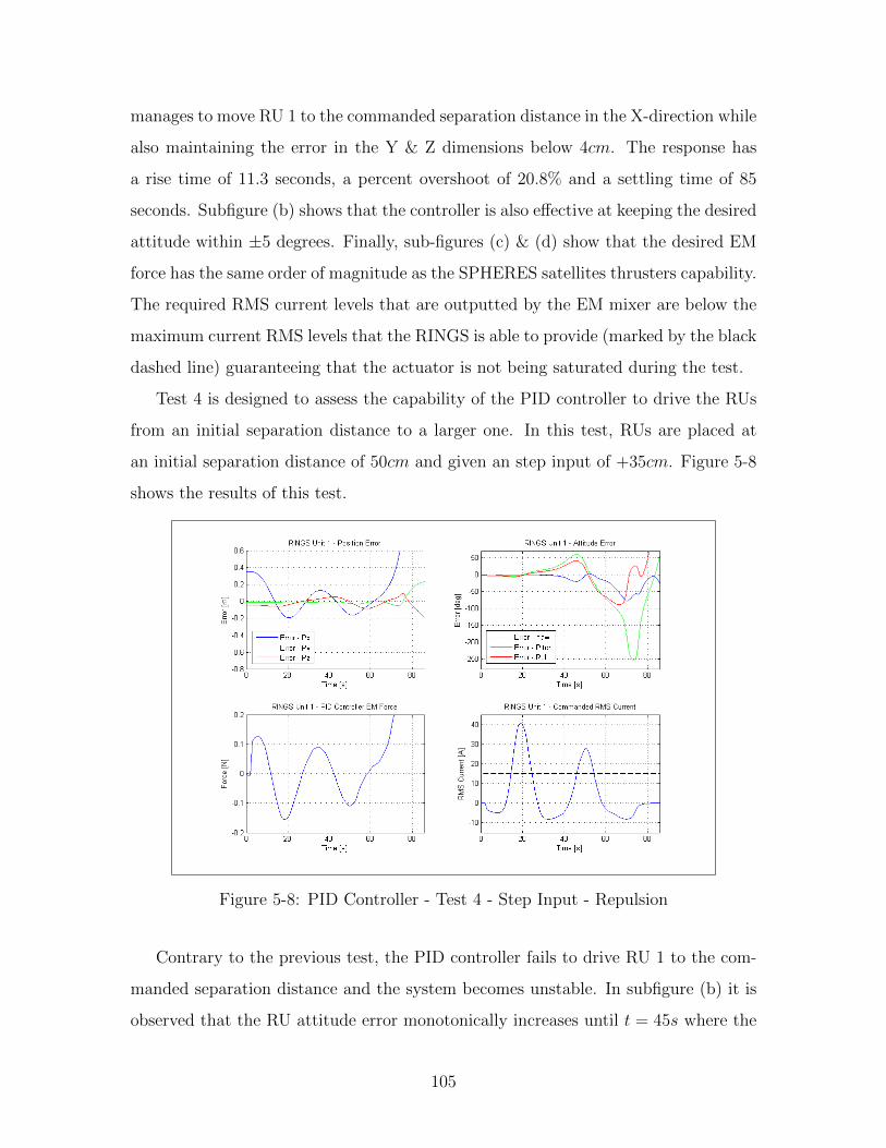
5-8 PID Controller - Test 4 - Step Input - Repulsion . . . . . . . . . . . . 105
5-9 EM PID Controller with ‘Input Shaping’ . . . . . . . . . . . . . . . . 106
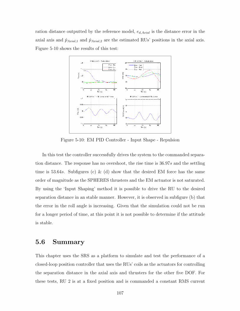
5-10 EM PID Controller - Input Shape - Repulsion . . . . . . . . . . . . . 107
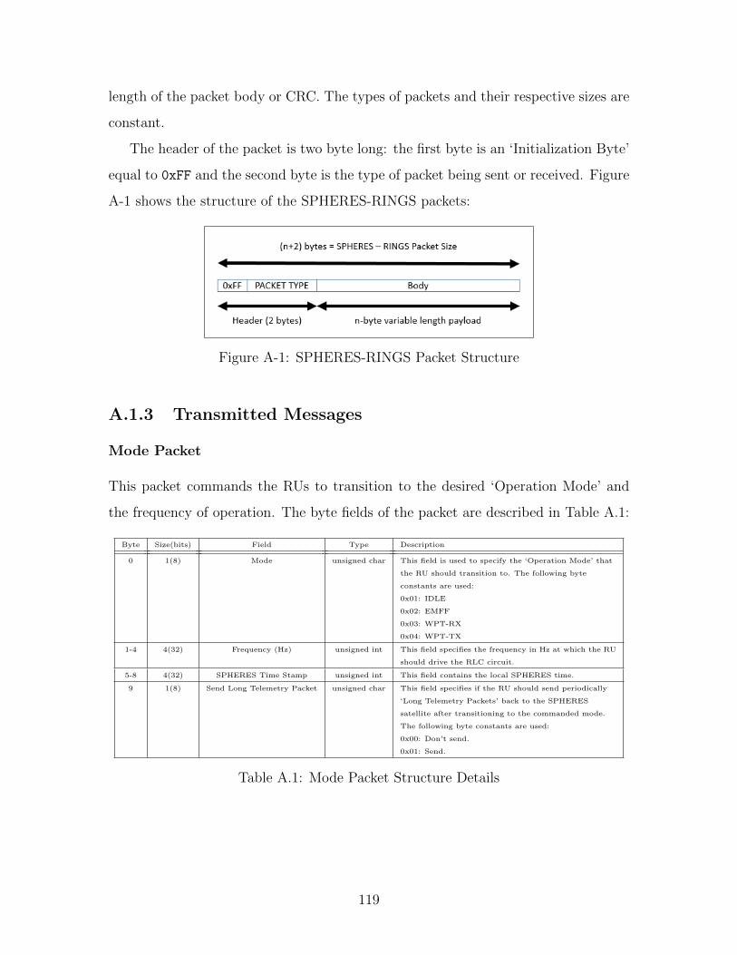
A-1 SPHERES-RINGS Packet Structure . . . . . . . . . . . . . . . . . . . 119
13
Page 17
List of Tables
2.1 Two-Coil PI Current Controller Model vs. Experiment - RMS Error . 45
3.1 SRS Output Variables . . . . . . . . . . . . . . . . . . . . . . . . . . 55
4.1 SPHERES-RINGS Moment of Inertia - Baseline . . . . . . . . . . . . 64
4.2 SPHERES-RINGS Center of Mass - Baseline . . . . . . . . . . . . . . 64
4.3 SPHERES Thrusters Torque Direction . . . . . . . . . . . . . . . . . 66
4.4 SPHERES-RINGS Moment of Inertia - ISS . . . . . . . . . . . . . . . 68
4.5 SPHERES-RINGS Center of Mass - ISS . . . . . . . . . . . . . . . . 69
4.6 SPHERES-RINGS Thrusters Force Matrix - ISS . . . . . . . . . . . . 69
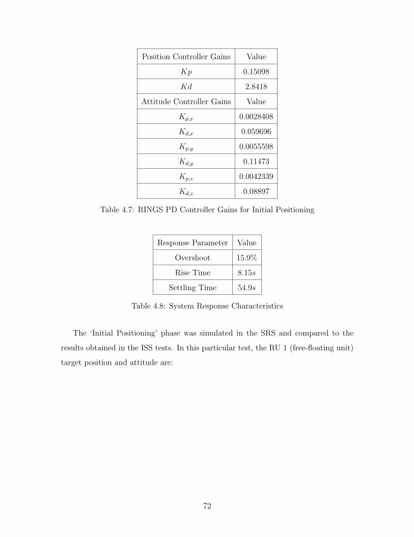
4.7 RINGS PD Controller Gains for Initial Positioning . . . . . . . . . . 72
4.8 System Response Characteristics . . . . . . . . . . . . . . . . . . . . 72
4.9 ‘Initial Positioning’ Phase - RU 1 Target Position and Attitude . . . . 73
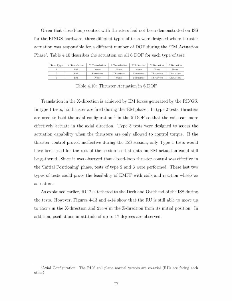
4.10 Thruster Actuation in 6 DOF . . . . . . . . . . . . . . . . . . . . . . 77
4.11 Drag Model Parameters . . . . . . . . . . . . . . . . . . . . . . . . . 81
4.12 ‘Current Model’ Parameters . . . . . . . . . . . . . . . . . . . . . . . 82
4.13 RINGS Hardware Verification - Additional Power . . . . . . . . . . . 86
5.1 CLPC Test Parameters . . . . . . . . . . . . . . . . . . . . . . . . . . 98
5.2 PID Controller Performance Comparison - Configuration A vs. B . . 104
A.1 Mode Packet Structure Details . . . . . . . . . . . . . . . . . . . . . . 119
A.2 PWM Packet Structure Details . . . . . . . . . . . . . . . . . . . . . 120
A.3 RMS Current Packet Structure Details . . . . . . . . . . . . . . . . . 120
A.4 Short Telemetry Packet Structure Details . . . . . . . . . . . . . . . . 121
15
Page 18
A.5 Long Telemetry Packet Structure Details . . . . . . . . . . . . . . . . 122
A.6 Operation Mode Acknowledgment Packet Structure Details . . . . . . 122
A.7 RINGS Units Sensor Gains and Physical Parameters . . . . . . . . . 123
A.8 Telemetry Data Conversion Factors . . . . . . . . . . . . . . . . . . . 123
16
Page 19
List of Acronyms and Initialisms
ADC - Analog to Digital ConverterAFS - Aurora Flight SciencesAI - Astronomical InterferometryCFD - Computational Fluid DynamicsCoM - Center of MassDARPA - Defense Advanced Research Projects AgencyDOF - Degree of FreedomDSP - Digital Signal ProcessorELC - Express Laptop ComputerEMF - Electromotive ForceEMFF - Electromagnetic Formation FlightESA - European Space AgencyEXPV2 - Expansion Port Version 2FFT - Fast Fourier TransformGMS - Global Metrology SystemGSP - Guest Scientist ProgramGUI - Graphical User InterfaceHES - Hall-Effect SensorHTS - High-Temperature SuperconductorIC - Integrated CircuitISS - International Space StationLEO - Low Earth OrbitMIT - Massachusetts Institute of TechnologyMOSFET - Metal-Oxide Field Effect TransistorNASA - National Aeronautics and Space AdministrationOS - Operating SystemPADS - Position and Attitude Determination SystemPD - Proportional-DerivativePID - Proportional-Integral-DerivativePWM - Pulse Width ModulationRGA - Reduced Gravity AircraftRINGS - Resonant Inductive Near-field Generation SystemRMS - Root Mean SquareRRM - Robotic Refueling MissionRTOS - Real-Time Operating SystemRU - RINGS Unit
17
Page 20
SIT - System Identification TestSK - Station KeepingSPDM - Special Purpose Dexterous ManipulatorSPHERES - Synchronized Position Hold Engage and Reorient Experimental SatellitesSRS - SPHERES-RINGS SimulationSSL - Space Systems LaboratoryTOF - Time of FlightTPF - Terrestrial Path FinderUART - Universal Asynchronous Receiver/TransmitterUMD - University of MarylandUS - Ultra SoundUSB - Universal Serial BusVERTIGO - Visual Estimation for Relative Tracking and Inspection of Generic ObjectsWPT - Wireless Power Transfer
18
Page 21
Chapter 1
Introduction
1.1 Motivations for Electromagnetic Formation Flight
(EMFF)
Electromagnetic Formation Flight (EMFF) consists of using electromagnetic forces
to position or orient satellites in a relative target location or attitude to achieve a
certain formation in orbit. Having this capability of keeping a cluster of satellites
with similar orbital parameters could enable multiple technologies:
1. Astronomical Interferometry (AI): Relies on an array of satellites in close prox-
imity to take images of a target location of a space body. By cross-referencing
these images, the angular resolution of the instrument is comparable to the one
that would be obtained by a single telescope with a much larger aperture. The
‘Darwin’ mission is an ESA study that consisted of a constellation of four to
nine spacecrafts to detect Earth-like planets orbiting nearby stars. However,
the development of this proposal was stopped in 2007 [6].
2. Fractionated Spacecraft Architecture: Brown et al. [7] proposed a new archi-
tectural paradigm called ‘Fractionated Spacecraft’ in which a satellite is de-
composed into different modules. These components communicate wirelessly to
achieve certain tasks while orbiting in a cluster. This architecture seeks not only
19
Page 22
to reduce program development time but also make the system more flexible
and robust to uncertainties.
3. Robotic Assembly: For some missions the aforementioned ‘Fractionated Archi-
tecture’ may not be a viable solution. In order to overcome limiting factors
imposed by size and weight of the spacecraft, a possible solution is to launch
modules separately and assemble them while in orbit using robots. Everist pro-
poses an experimental system for assembly in space [8]. As an example, the
Special Purpose Dexterous Manipulator (SPDM), a two armed robot aboard
the ISS, has been used in the Robotic Refueling Mission (RRM) to show its
capability to perform tasks such as unscrew caps and adjust valves of a module
that was not originally designed to be serviced [9].
Multiple technologies can be used to correct for disturbances and achieve a target
formation. One solution is to use thrusters as the actuation system. However, given
that spacecrafts can only carry a limited amount of propellant this solution poses a
limitation in the operational lifetime of the cluster. A second alternative is to use
tethers between the spacecrafts that form the cluster. However, this solution requires
the deployment of tethers in space which has proven to be an extremely difficult task
that limits the possible orientations of the cluster.
In EMFF magnetic fields are generated by the different nodes of the cluster. The
interaction of these fields generate electromagnetic forces and torques that are used
to control and maintain the formation. Due to the Conservation of Momentum and
the fact that all the electromagnetic forces generated are internal to the cluster, its
center of mass (CoM) cannot change. Thus, the EMFF approach can only be used
to control the relative position and attitude of the spacecraft.
EMFF has three major advantages over the aforementioned solutions. This tech-
nology is propellant-free since the electrical currents required to generate the magnetic
fields can be obtained from sustainable sources such as batteries that are charged us-
ing solar panels. Thus, the operational lifetime constraint would be eliminated since
the system would have a replenishable power source. The second major advantage is
20
Page 23
for missions that have payloads with optical sensors that can be damaged by propel-
lants. As an example, the Terrestrial Path Finder (TPF) mission utilizes an infrared
interferometer to detect an Earth-like planet [10]. In this mission a cluster of satellites
rotate in close proximity and the plume of the thrusters could cloud the sensors.
A complementary application of EMFF is Wireless Power Transfer (WPT). WPT
consists in generating an alternating magnetic field to transfer energy to another
device wirelessly. This technology adds flexibility to the mission architecture since
some spacecraft in the cluster could only be responsible for power generation and
distribution while other spacecraft could be specialized in the science objective and
be powered remotely.
1.2 Previous Work
1.2.1 EMFF Control
A significant amount of work on EMFF control has been published. The concept of
using electromagnetic forces for space Formation Flight in Low Earth Orbit (LEO)
is originally presented in series of papers by Hashimoto, Sakai, Ninomiya, et al. [11].
Elias [12] developed an EMFF dynamics model that considered satellites to have
a fully controllable dipole and showed closed loop controllability of the system. Satel-
lites are assumed to be a distance great enough from each other that they can be
modeled as magnetic dipoles.
In his thesis, Schweighart [3] developed three models for EM forces and torques,
namely ‘Near-Field’, ‘Mid-Field’ and ‘Far-Field’. In his work, closed form solutions
for the ‘Mid-Field’ and ‘Far-Field’ are derived and control methods for multi-satellite
clusters are given.
Wawrzaszek et al. [13] developed a linear model for a two-satellite cluster that
performs a spin-up maneuver. Their work proves that feedback control is required for
system stability and a linear controller is shown to stabilize the system for a range of
disturbances.
21
Page 24
1.2.2 EMFF Testbeds
Since 2004, multiple testbeds have been developed in the Space Systems Laboratory
(SSL) at MIT:
1. In 2004, a 1-Dimensional EMFF testbed was created [12]. It featured one
electromagnet fixed at one end of a linear track while a second electromagnet
was able to float in the track. By changing the current in the magnets and using
an ultrasonic device to measure position, it was possible to control the position
of the magnet floating on the track.
2. In 2005, a 2-Dimensional EMFF testbed (3 DoF) was created [14]. It consisted
of two vehicles that floated on a flat floor using air carriages. Each vehicle was
equipped with two coils that were orthogonal to each other. The material used
was High-Temperature Superconducting wire (HTS) to allow the circulation of
high levels of current and generation of appreciable forces.
3. A 1-Dimensional testbed, known as µEMFF [15], used two non-superconducting
coils to test different control algorithms and demonstrate the possibility of
achieving EMFF using non-superconducting electromagnets.
1.3 Resonant Inductive Near-Field Generation Sys-
tem (RINGS)
The Resonant Inductive Near-Field Generation System (RINGS) is an experimental
testbed to demonstrate EMFF and WPT in a micro-gravity environment. RINGS is
composed of two vehicles, referred to as RINGS units (RUs), that integrate to the
Synchronized, Position Hold, Engage, Reorient, Experimental Satellites (SPHERES)
and was launched to the International Space Station (ISS) in August 2013. SPHERES
satellites are placed on the center of the RU and are equipped with their own propul-
sion, power and navigation system. These satellites are capable of being programmed
22
Page 25
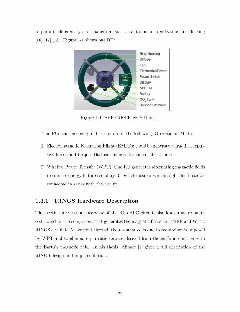
to perform different type of maneuvers such as autonomous rendezvous and docking
[16] [17] [18]. Figure 1-1 shows one RU:
Figure 1-1: SPHERES-RINGS Unit [1]
The RUs can be configured to operate in the following ‘Operational Modes’:
1. Electromagnetic Formation Flight (EMFF): the RUs generate attractive, repul-
sive forces and torques that can be used to control the vehicles.
2. Wireless Power Transfer (WPT): One RU generates alternating magnetic fields
to transfer energy to the secondary RU which dissipates it through a load resistor
connected in series with the circuit.
1.3.1 RINGS Hardware Description
This section provides an overview of the RUs RLC circuit, also known as ‘resonant
coil’, which is the component that generates the magnetic fields for EMFF and WPT.
RINGS circulate AC current through the resonant coils due to requirements imposed
by WPT and to eliminate parasitic torques derived from the coil’s interaction with
the Earth’s magnetic field. In his thesis, Alinger [2] gives a full description of the
RINGS design and implementation.
23
Page 26
RLC Circuit
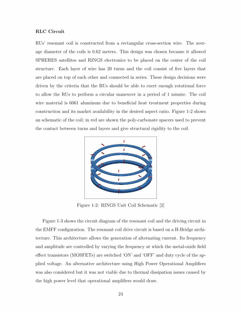
RUs’ resonant coil is constructed from a rectangular cross-section wire. The aver-
age diameter of the coils is 0.62 meters. This design was chosen because it allowed
SPHERES satellites and RINGS electronics to be placed on the center of the coil
structure. Each layer of wire has 20 turns and the coil consist of five layers that
are placed on top of each other and connected in series. These design decisions were
driven by the criteria that the RUs should be able to exert enough rotational force
to allow the RUs to perform a circular maneuver in a period of 1 minute. The coil
wire material is 6061 aluminum due to beneficial heat treatment properties during
construction and its market availability in the desired aspect ratio. Figure 1-2 shows
an schematic of the coil; in red are shown the poly-carbonate spacers used to prevent
the contact between turns and layers and give structural rigidity to the coil.
Figure 1-2: RINGS Unit Coil Schematic [2]
Figure 1-3 shows the circuit diagram of the resonant coil and the driving circuit in
the EMFF configuration. The resonant coil drive circuit is based on a H-Bridge archi-
tecture. This architecture allows the generation of alternating current. Its frequency
and amplitude are controlled by varying the frequency at which the metal-oxide field
effect transistors (MOSFETs) are switched ‘ON’ and ‘OFF’ and duty cycle of the ap-
plied voltage. An alternative architecture using High Power Operational Amplifiers
was also considered but it was not viable due to thermal dissipation issues caused by
the high power level that operational amplifiers would draw.
24
Page 27
Figure 1-3: RLC Circuit Diagram [2]
EMFF operational frequency was desired to be as low as possible. Given physical,
thermal and operational design constraints, a 310uF capacitor was chosen for the
EMFF configuration. From experimental results obtained by Alinger et al. [2] it was
determined that for frequencies lower than 1kHz, the inductance and resistance of
the RUs’ resonant coils are:
L = 11.9mH
R = 1.1Ω
Given these values, the resonant frequency of the RLC circuit in the EMFF con-
figuration is:
fEMFF =1
2π√LC
=1
2π√
11.9mH ∗ 310µF= 82.90Hz ≈ 83Hz
Current Sensors
The current that flows through the resonant coils is measured by ACS709LLFTR-
20BB-T Hall-Effect sensors (HES) manufactured by Allegro Microsystems. For re-
dundancy, three HESs are in series with the circuit. In addition, the RUs are equipped
25
Page 28
with a pair of LTC1968 RMS-to-DC converters manufactured by Linear Technology.
1.3.2 RINGS Firmware
RUs are equipped with a PIC32MX340F512H manufactured by Microchip. Given the
existing capabilities and software infrastructure in SPHERES, it was decided that the
functional requirements of the firmware would be to:
1. Configure the internal RLC circuit to the different operational modes: IDLE,
EMFF, WPT-TX, WPT-RX.
2. Drive the current flowing through the coils to a commanded RMS level.
3. Synchronize the current waves using the IR pulses received.
4. Receive measurements from the system sensors and change to any ‘Error Mode’
accordingly.
5. Send acknowledgement messages and telemetry data back to the SPHERES
satellite.
1.3.3 EMFF Near-Field Dynamics Model
Models of EM forces and torques can be classified into three major categories accord-
ing to the relative distance between the spacecraft that are generating the magnetic
fields:
1. Near-Field Model: Is the exact solution to the magnetic forces and torques
generated in an EMFF system.
2. Far-Field Model: When the vehicles are sufficiently far away, they can be mod-
eled as point magnetic dipoles and their exact geometry can be ignored. This
model is the first order Taylor series expansion of the force between the two
vehicles.
26
Page 29
3. Mid-Field Model: For situations in which satellites need to operate in close
proximity, the Far-Field model is inaccurate. The Mid-Field model incorporates
the next higher order expansion of the Taylor series.
RINGS operates in the SPHERES test volume aboard the ISS. Thus, given the
small operational distances between the vehicles the Far-Field model assumption does
not hold and the Near-Field model must be used instead. The rest of this section
describes the governing equations of the Near-Field model.
According to the ‘Lorentz Force Law’, a continuous charge distribution in motion
in the presence of a magnetic field can be described by the following equation:
d~F = i~dl × ~B (1.1)
By applying equation 1.1, Biot-Savart’s Law and Faraday’s Law the resulting EM
force and torque of two loops carrying current are [3]:
Fij =µ0IiIj
4π
∮i
∮j
~dli ×(~dlj × rij
)‖~r2‖
(1.2)
τij =µ0IiIj
4π
∮i
∮j
~Ri ×~dli ×
(~dlj × rij
)‖~r2‖
(1.3)
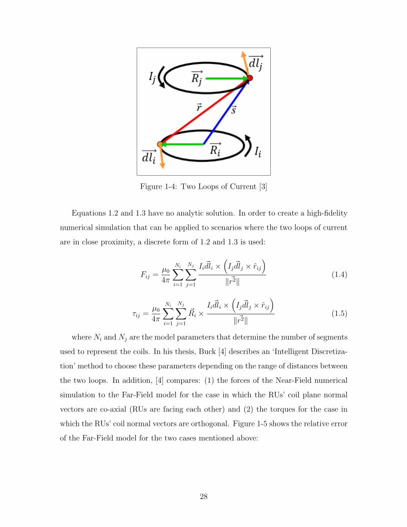
where Fij and τij are the resulting force and torque on loop i due to loop j
respectively, µ0 is the permeability of free space and ~dli is an infinitesimal length of
conductor i. Equations 1.2 and 1.3 assume that all segments of loop i and j carry
the same level of current Ii and Ij respectively. ~Ri is the position vector of element
~dli relative to the center of mass of object i as shown in Figure 1-4:
27
Page 30
Figure 1-4: Two Loops of Current [3]
Equations 1.2 and 1.3 have no analytic solution. In order to create a high-fidelity
numerical simulation that can be applied to scenarios where the two loops of current
are in close proximity, a discrete form of 1.2 and 1.3 is used:
Fij =µ0
4π
Ni∑i=1
Nj∑j=1
Ii~dli ×(Ij ~dlj × rij
)‖~r2‖
(1.4)
τij =µ0
4π
Ni∑i=1
Nj∑j=1
~Ri ×Ii~dli ×
(Ij ~dlj × rij
)‖~r2‖
(1.5)
where Ni and Nj are the model parameters that determine the number of segments
used to represent the coils. In his thesis, Buck [4] describes an ‘Intelligent Discretiza-
tion’ method to choose these parameters depending on the range of distances between
the two loops. In addition, [4] compares: (1) the forces of the Near-Field numerical
simulation to the Far-Field model for the case in which the RUs’ coil plane normal
vectors are co-axial (RUs are facing each other) and (2) the torques for the case in
which the RUs’ coil normal vectors are orthogonal. Figure 1-5 shows the relative error
of the Far-Field model for the two cases mentioned above:
28
Page 31
Figure 1-5: Near vs Far-Field - Relative Error for Axial Force and Shear Torque [4]
In Figure 1-5 the X-axis is normalized to the RUs’ radius. It is shown that at 7
radii (approximately 2.1 meters), the relative error between the Far-Field and Near-
Field models is above 10%. Thus, for the operational distances of RINGS the figure
above proves that the Far-Field model is not applicable and the Near-Field model
has to be used instead.
1.4 Thesis Overview
The majority of this thesis involves the development and validation of a simulation
of RINGS. In addition, closed-loop controllers for RINGS are developed and tested
in simulation to achieve position control. This work is organized as follows:
Chapter 2 explains the motivation for a current controller for RINGS. A model
of a PI Current Controller for RINGS is developed. The behavior of the system
is simulated in SIMULINK and then compared to experiments performed on the
engineering RUs. The objective of these experiments is to study the response
and stability of the system when using a PI current controller.
Chapter 3 starts by describing the SPHERES simulation developed by Katz [5].
29
Page 32
Then, it presents the development of the SPHERES-RINGS Simulation (SRS)
and a description of the different components and their integration with the
SPHERES simulation.
Chapter 4’s objective is to validate the SRS developed in the previous chapter by
comparing experimental data obtained aboard the ISS with simulation results.
Partial results show the necessity to modify the initial version of the SRS and
a justification for these modifications are given.
Chapter 5 develops a closed-loop position controller that uses EM actuation
for a single axis and SPHERES thrusters for the other 5 DoF. This controller
is simulated in the SRS to test the stability of the system. Due to the insta-
bility observed in certain maneuvers, an ‘Adaptive Control’ method known as
‘Reference Input’ is implemented and tested to achieve stability of the system.
Chapter 6 summarizes the conclusions of this work and it suggests future steps
for the progress of the RINGS program and the demonstration of EMFF in a
micro-gravity environment.
30
Page 33
Chapter 2
Modeling and Implementation of a
PI Current Controller for RINGS
2.1 Introduction
This chapter describes the motivation, development and testing of a Proportional-
Integrator current controller for the RINGS. Initially, a ‘One-Coil Model’ was imple-
mented in Simulink to test the performance of the PI controller. In this model only
one RU with a PI controller is simulated. Then a ‘Two-Coil Model’ was developed to
study the impact that inductive coupling between two RUs has in the performance
of the PI controller. The simulation results are also compared against experimental
tests performed in the ground testbed.
2.2 Motivation
Equations 1.2 and 1.3 show that the EM force and torque are directly proportional
to the loop currents i1 and i2. Given that the frequency of the sinusoidal field for
EMFF (83Hz) is fast when compared to the rigid body motion, the average result
across time is identical to a non-oscillating system driven at the Root Mean Square
(RMS) level of the sinusoidal system. Thus, the control variable of interest becomes
the RMS current level flowing in the loops.
31
Page 34
The RUs’ RLC circuit is driven by controlling an H-bridge (see Section 1.3.1),
using a PWM signal to generate alternate voltage and subsequently control the level
and frequency of the current flowing through the circuit (see Figure 1-3). With this
architecture, using Fourier series expansions, the steady-state current is:
Iss(t) = VBatt
∞∑n=1
Dn |Gn| cos(
2πn
Tt− φn + 6 Gn
)(2.1)
where Gn is the RLC circuit transfer function and:
Dn =√A2
n +B2n
φn = tan−1(Bn
An
)An =
2
nπsin
(πnt
T
)(cos
(πnt
T
)− cos
(πn (t− T )
T
))Bn =
2
nπsin
(πnt
T
)(sin
(πnt
T
)− sin
(πn (t− T )
T
))Gn =
1
jωnL(ωn) +R(ωn) + 1jωnC
Equation 2.1 shows that the current is directly proportional to raw battery voltage
VBatt. As the RU uses battery’s energy, VBatt decreases and for a given Duty Cycle
(DC) the Iss will also decrease. Figure 2-1 shows simulation results performed by
Alinger [2] where the effect on Iss when varying VBatt is assessed:
Figure 2-1: Iss vs. Duty Cycle for different (VBatt) [2]
32
Page 35
It is observed that the battery voltage has a significant effect on the RMS current.
For example, at 60% DC, the RMS current decreases by 17% (from 20A to 16.7A)
when VBatt decreases from 36V to 30V.
In addition to the fluctuation of the battery voltage, the level of current flowing
though the coils will be affected by the ‘inductive coupling’. According to Faraday’s
Law of Induction, the time rate of change of the magnetic flux through the circuit will
induce an Electromotive Force (EMF) in any other closed circuit. The magnitude of
the EMF is proportional to the time rate of change of the magnetic flux, the RUs coil
inductance, and the coupling coefficient. The coupling coefficient, κ, is a geometric
constant between 0 and 1 that represents the effective magnetic flux that goes through
the second RU’s coil. Thus, the change in current in one RU will create a disturbance
on the current level of the second RU and vice versa.
2.3 Proportional-Integrator (PI) Controller
From the previous discussion, it was decided to develop a PI current controller that is
capable of maintaining a reference RMS current level and is robust to the disturbances
created by the inductive coupling. The equation for a PI controller is:
C (t) = KP ∗ E (t) +KI ∗∫ t
0
E(t)dt (2.2)
where KP and KI are the proportional and integral gains respectively. Given that
the PI controller will be digital, the integral term was approximated using:
∫ t
0
E(t)dt ≈ TS
N∑n=0
E(n) (2.3)
where TS is the sampling period. The equation for the PI controller becomes:
C(n) = KP ∗ E(n) +KI ∗ TSN∑
n=0
E(n) (2.4)
33
Page 36
2.4 ‘Ziegler-Nichols’ Method for Tuning PI Con-
troller Gains
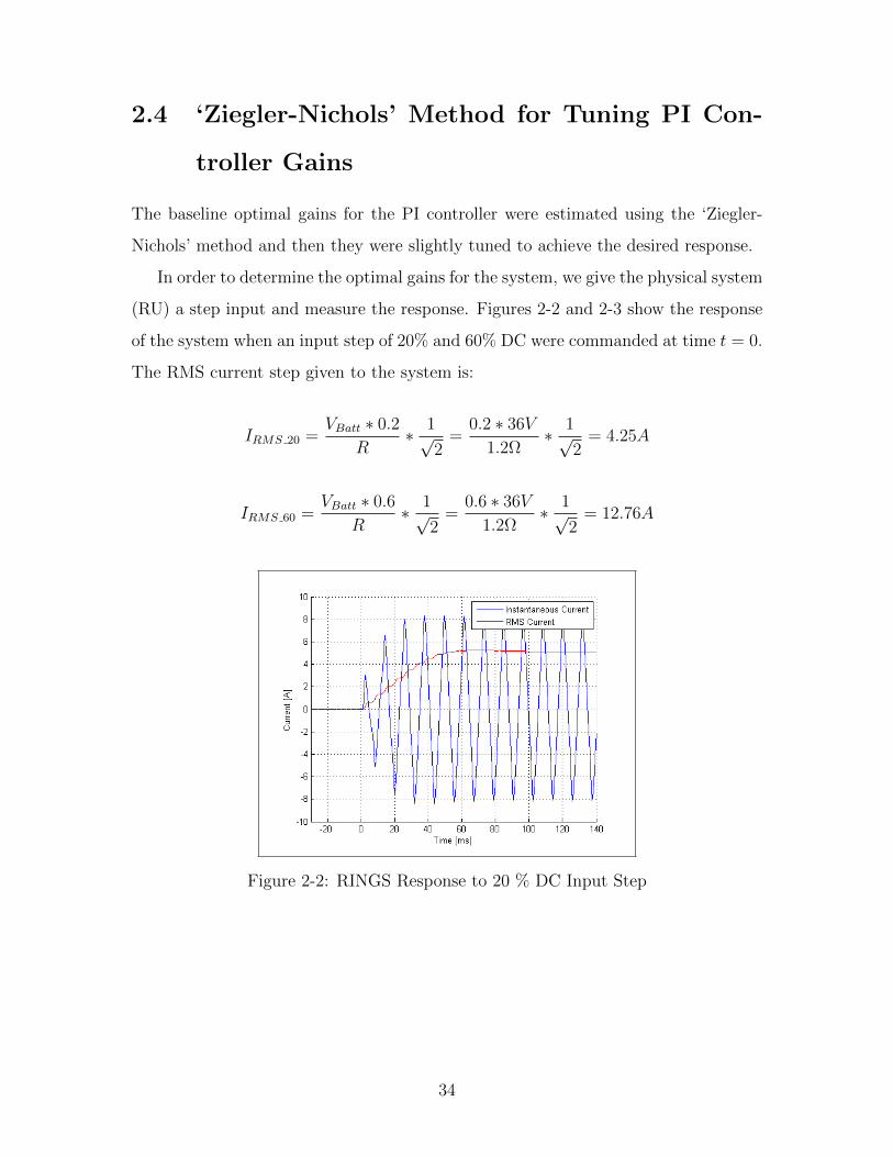
The baseline optimal gains for the PI controller were estimated using the ‘Ziegler-
Nichols’ method and then they were slightly tuned to achieve the desired response.
In order to determine the optimal gains for the system, we give the physical system
(RU) a step input and measure the response. Figures 2-2 and 2-3 show the response
of the system when an input step of 20% and 60% DC were commanded at time t = 0.
The RMS current step given to the system is:
IRMS 20 =VBatt ∗ 0.2
R∗ 1√
2=
0.2 ∗ 36V
1.2Ω∗ 1√
2= 4.25A
IRMS 60 =VBatt ∗ 0.6
R∗ 1√
2=
0.6 ∗ 36V
1.2Ω∗ 1√
2= 12.76A
Figure 2-2: RINGS Response to 20 % DC Input Step
34
Page 37
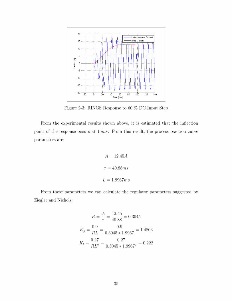
Figure 2-3: RINGS Response to 60 % DC Input Step
From the experimental results shown above, it is estimated that the inflection
point of the response occurs at 15ms. From this result, the process reaction curve
parameters are:
A = 12.45A
τ = 40.88ms
L = 1.9967ms
From these parameters we can calculate the regulator parameters suggested by
Ziegler and Nichols:
R =A
τ=
12.45
40.88= 0.3045
Kp =0.9
RL=
0.9
0.3045 ∗ 1.9967= 1.4803
Kt =0.27
RL2=
0.27
0.3045 ∗ 1.99672= 0.222
35
Page 38
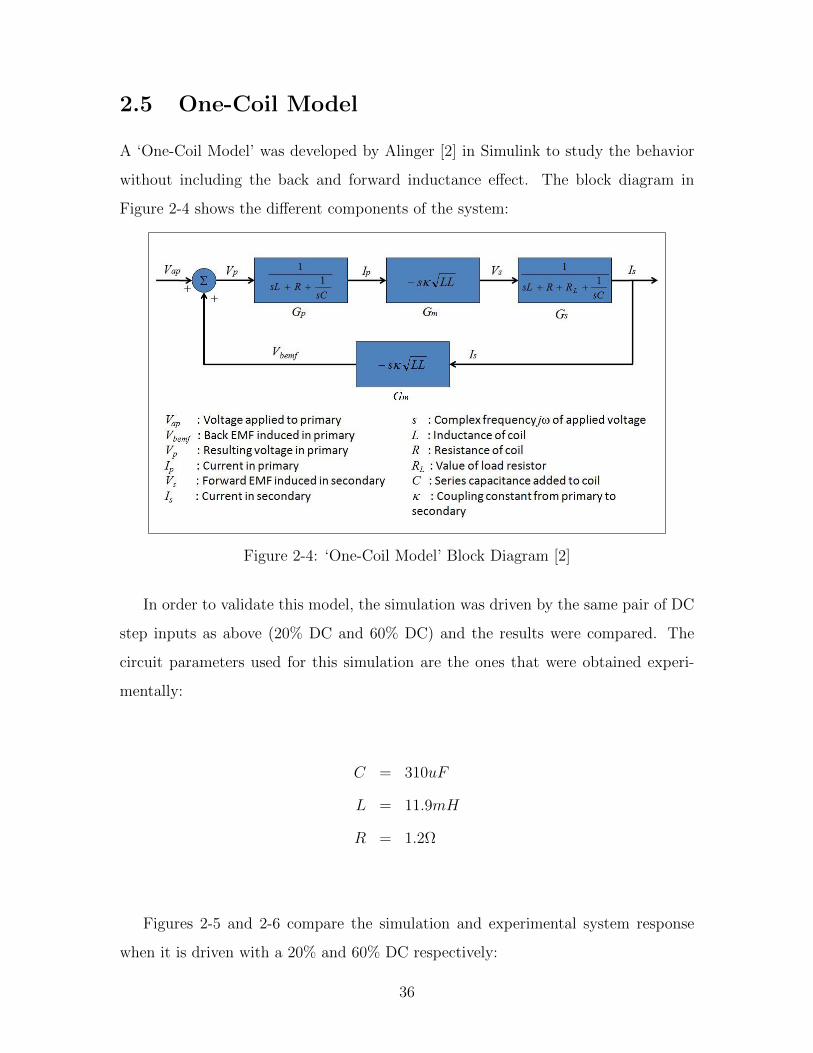
2.5 One-Coil Model
A ‘One-Coil Model’ was developed by Alinger [2] in Simulink to study the behavior
without including the back and forward inductance effect. The block diagram in
Figure 2-4 shows the different components of the system:
Figure 2-4: ‘One-Coil Model’ Block Diagram [2]
In order to validate this model, the simulation was driven by the same pair of DC
step inputs as above (20% DC and 60% DC) and the results were compared. The
circuit parameters used for this simulation are the ones that were obtained experi-
mentally:
C = 310uF
L = 11.9mH
R = 1.2Ω
Figures 2-5 and 2-6 compare the simulation and experimental system response
when it is driven with a 20% and 60% DC respectively:
36
Page 39
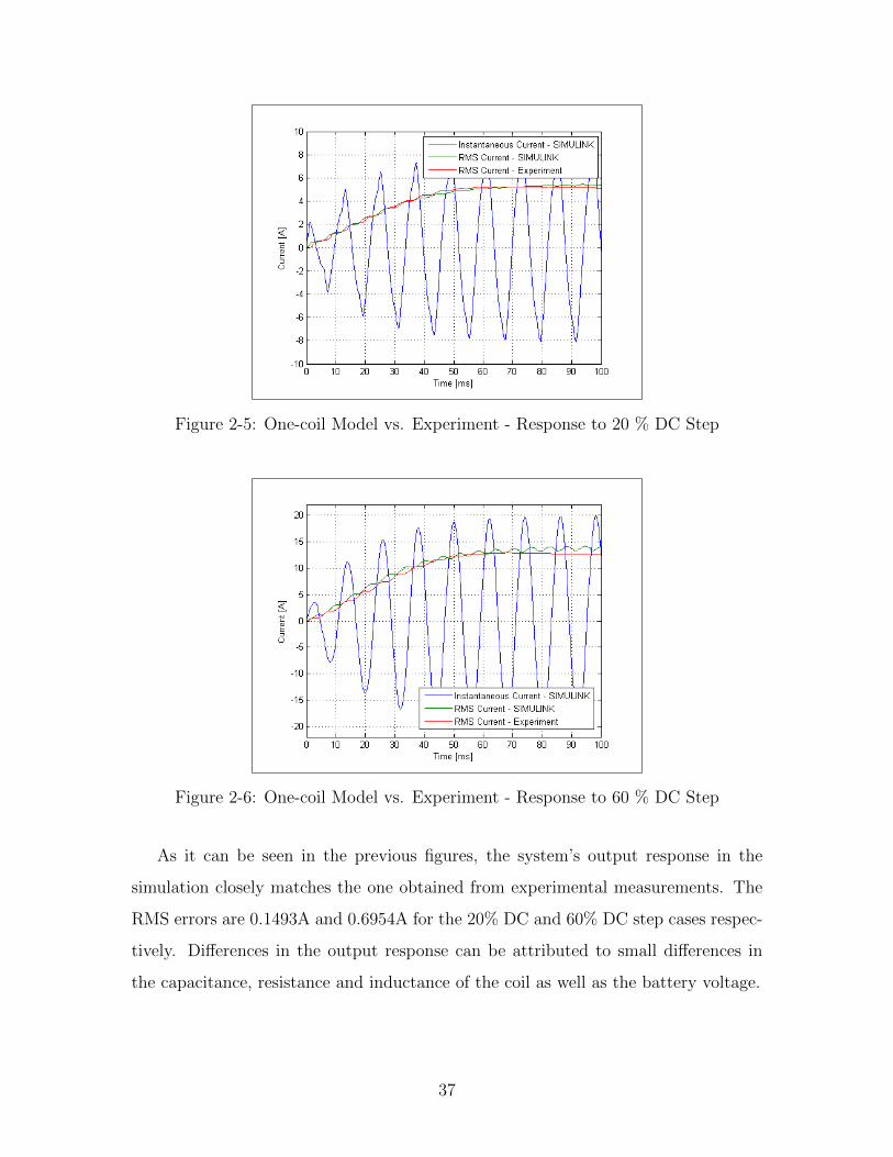
Figure 2-5: One-coil Model vs. Experiment - Response to 20 % DC Step
Figure 2-6: One-coil Model vs. Experiment - Response to 60 % DC Step
As it can be seen in the previous figures, the system’s output response in the
simulation closely matches the one obtained from experimental measurements. The
RMS errors are 0.1493A and 0.6954A for the 20% DC and 60% DC step cases respec-
tively. Differences in the output response can be attributed to small differences in
the capacitance, resistance and inductance of the coil as well as the battery voltage.
37
Page 40
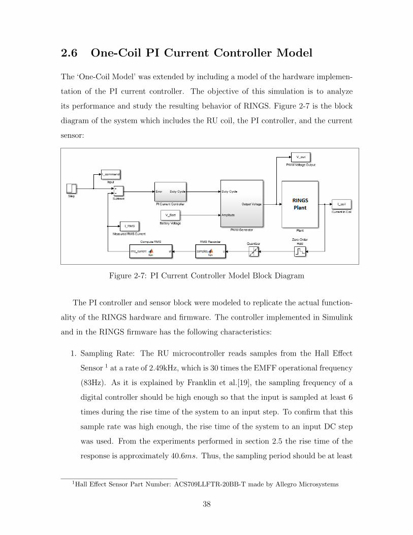
2.6 One-Coil PI Current Controller Model
The ‘One-Coil Model’ was extended by including a model of the hardware implemen-
tation of the PI current controller. The objective of this simulation is to analyze
its performance and study the resulting behavior of RINGS. Figure 2-7 is the block
diagram of the system which includes the RU coil, the PI controller, and the current
sensor:
Figure 2-7: PI Current Controller Model Block Diagram
The PI controller and sensor block were modeled to replicate the actual function-
ality of the RINGS hardware and firmware. The controller implemented in Simulink
and in the RINGS firmware has the following characteristics:
1. Sampling Rate: The RU microcontroller reads samples from the Hall Effect
Sensor 1 at a rate of 2.49kHz, which is 30 times the EMFF operational frequency
(83Hz). As it is explained by Franklin et al.[19], the sampling frequency of a
digital controller should be high enough so that the input is sampled at least 6
times during the rise time of the system to an input step. To confirm that this
sample rate was high enough, the rise time of the system to an input DC step
was used. From the experiments performed in section 2.5 the rise time of the
response is approximately 40.6ms. Thus, the sampling period should be at least
1Hall Effect Sensor Part Number: ACS709LLFTR-20BB-T made by Allegro Microsystems
38
Page 41
6.77ms or equivalently 150Hz. The sampling frequency chosen for RINGS was
higher than 150Hz due to system requirements of the WPT operation mode.
2. Quantization: The RU PIC microcontroller is equipped with a 10-bit Analog-to-
Digital converter. This characteristic was incorporated in the model by quan-
tizing the output signal of the HES.
3. Using the last 90 measured current values, the RMS current value is computed
and fed back to the PI controller.
4. PWM Generation Module: The RINGS firmware has a resolution of 0.005 to
set the duty cycle of the PWM signal. Thus, the output DC of the current
controller is converted to the closest value that can be resolved.
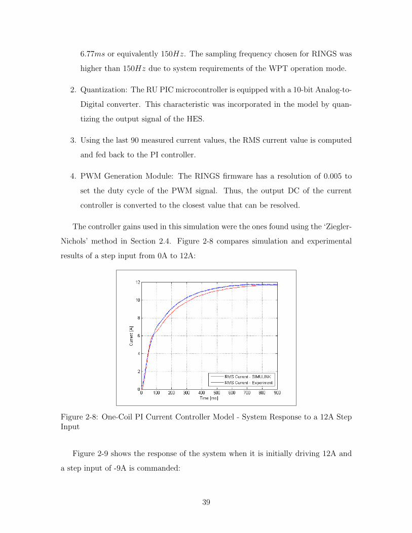
The controller gains used in this simulation were the ones found using the ‘Ziegler-
Nichols’ method in Section 2.4. Figure 2-8 compares simulation and experimental
results of a step input from 0A to 12A:
Figure 2-8: One-Coil PI Current Controller Model - System Response to a 12A StepInput
Figure 2-9 shows the response of the system when it is initially driving 12A and
a step input of -9A is commanded:
39
Page 42
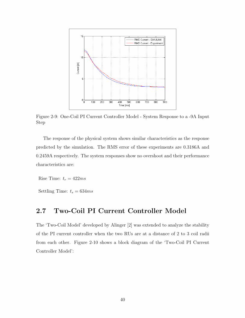
Figure 2-9: One-Coil PI Current Controller Model - System Response to a -9A InputStep
The response of the physical system shows similar characteristics as the response
predicted by the simulation. The RMS error of these experiments are 0.3186A and
0.2459A respectively. The system responses show no overshoot and their performance
characteristics are:
Rise Time: tr = 422ms
Settling Time: ts = 634ms
2.7 Two-Coil PI Current Controller Model
The ‘Two-Coil Model’ developed by Alinger [2] was extended to analyze the stability
of the PI current controller when the two RUs are at a distance of 2 to 3 coil radii
from each other. Figure 2-10 shows a block diagram of the ‘Two-Coil PI Current
Controller Model’:
40
Page 43
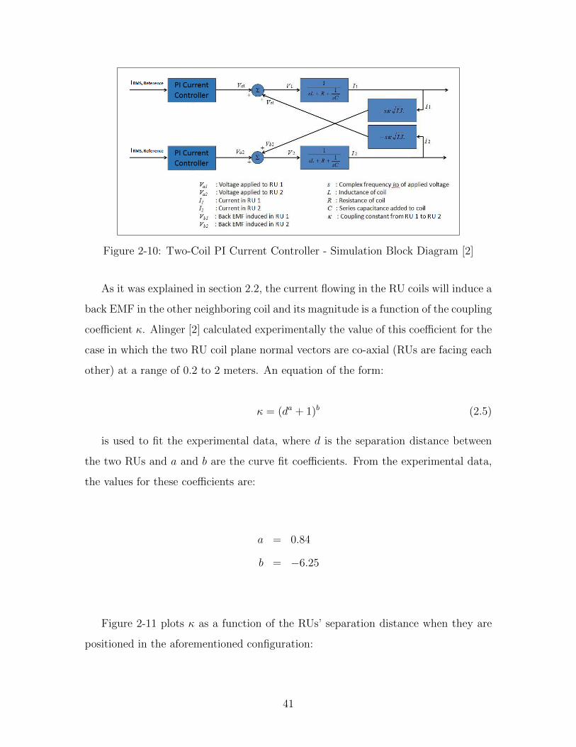
Figure 2-10: Two-Coil PI Current Controller - Simulation Block Diagram [2]
As it was explained in section 2.2, the current flowing in the RU coils will induce a
back EMF in the other neighboring coil and its magnitude is a function of the coupling
coefficient κ. Alinger [2] calculated experimentally the value of this coefficient for the
case in which the two RU coil plane normal vectors are co-axial (RUs are facing each
other) at a range of 0.2 to 2 meters. An equation of the form:
κ = (da + 1)b (2.5)
is used to fit the experimental data, where d is the separation distance between
the two RUs and a and b are the curve fit coefficients. From the experimental data,
the values for these coefficients are:
a = 0.84
b = −6.25
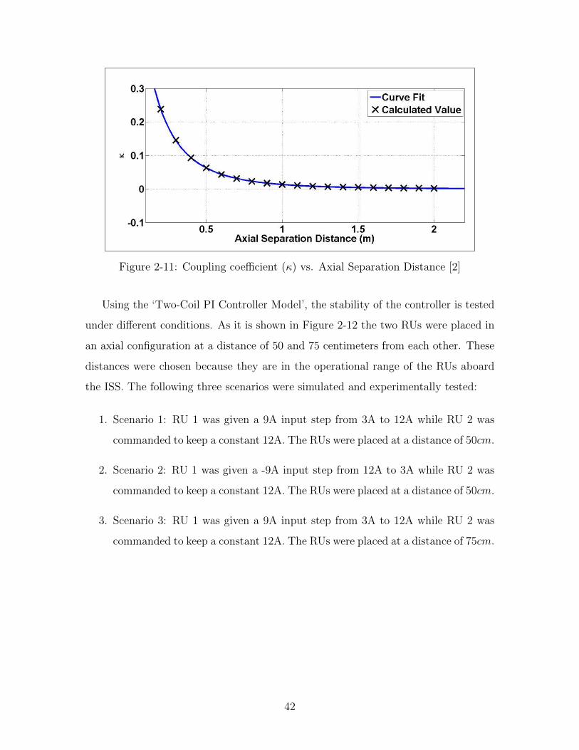
Figure 2-11 plots κ as a function of the RUs’ separation distance when they are
positioned in the aforementioned configuration:
41
Page 44
Figure 2-11: Coupling coefficient (κ) vs. Axial Separation Distance [2]
Using the ‘Two-Coil PI Controller Model’, the stability of the controller is tested
under different conditions. As it is shown in Figure 2-12 the two RUs were placed in
an axial configuration at a distance of 50 and 75 centimeters from each other. These
distances were chosen because they are in the operational range of the RUs aboard
the ISS. The following three scenarios were simulated and experimentally tested:
1. Scenario 1: RU 1 was given a 9A input step from 3A to 12A while RU 2 was
commanded to keep a constant 12A. The RUs were placed at a distance of 50cm.
2. Scenario 2: RU 1 was given a -9A input step from 12A to 3A while RU 2 was
commanded to keep a constant 12A. The RUs were placed at a distance of 50cm.
3. Scenario 3: RU 1 was given a 9A input step from 3A to 12A while RU 2 was
commanded to keep a constant 12A. The RUs were placed at a distance of 75cm.
42
Page 45
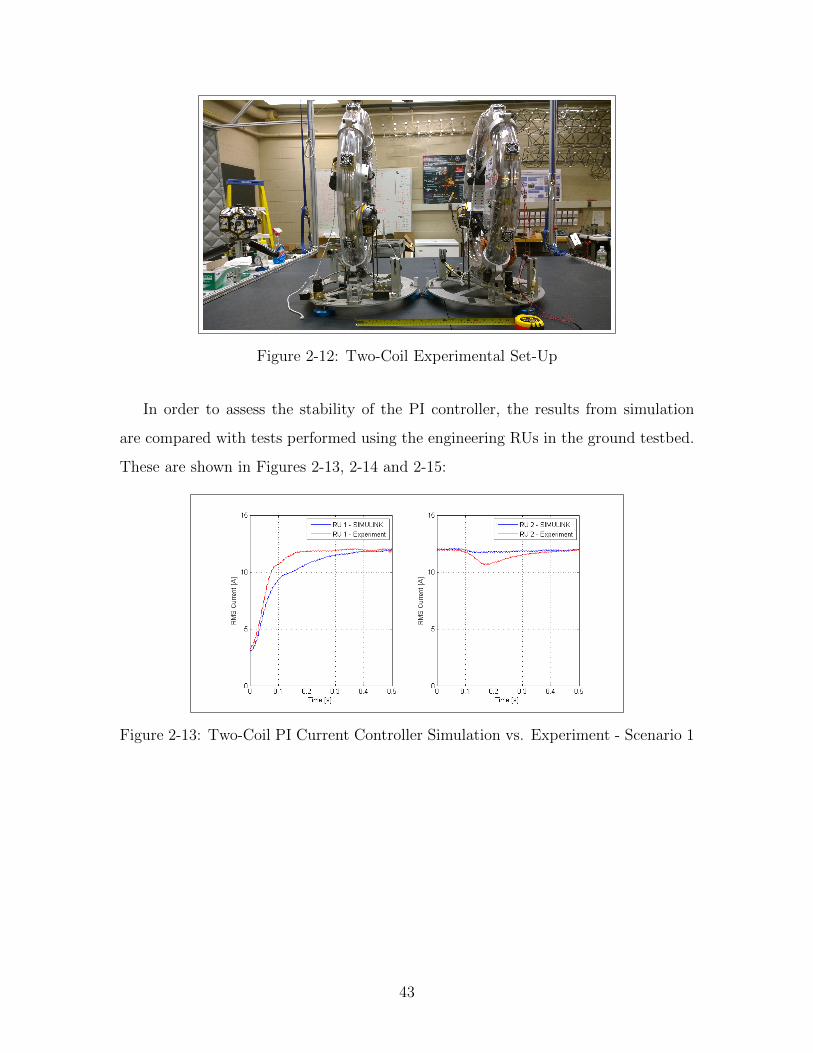
Figure 2-12: Two-Coil Experimental Set-Up
In order to assess the stability of the PI controller, the results from simulation
are compared with tests performed using the engineering RUs in the ground testbed.
These are shown in Figures 2-13, 2-14 and 2-15:
Figure 2-13: Two-Coil PI Current Controller Simulation vs. Experiment - Scenario 1
43
Page 46
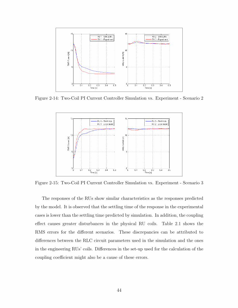
Figure 2-14: Two-Coil PI Current Controller Simulation vs. Experiment - Scenario 2
Figure 2-15: Two-Coil PI Current Controller Simulation vs. Experiment - Scenario 3
The responses of the RUs show similar characteristics as the responses predicted
by the model. It is observed that the settling time of the response in the experimental
cases is lower than the settling time predicted by simulation. In addition, the coupling
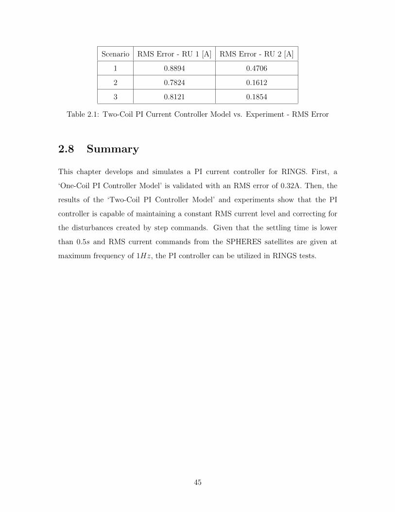
effect causes greater disturbances in the physical RU coils. Table 2.1 shows the
RMS errors for the different scenarios. These discrepancies can be attributed to
differences between the RLC circuit parameters used in the simulation and the ones
in the engineering RUs’ coils. Differences in the set-up used for the calculation of the
coupling coefficient might also be a cause of these errors.
44
Page 47
Scenario RMS Error - RU 1 [A] RMS Error - RU 2 [A]
1 0.8894 0.4706
2 0.7824 0.1612
3 0.8121 0.1854
Table 2.1: Two-Coil PI Current Controller Model vs. Experiment - RMS Error
2.8 Summary
This chapter develops and simulates a PI current controller for RINGS. First, a
‘One-Coil PI Controller Model’ is validated with an RMS error of 0.32A. Then, the
results of the ‘Two-Coil PI Controller Model’ and experiments show that the PI
controller is capable of maintaining a constant RMS current level and correcting for
the disturbances created by step commands. Given that the settling time is lower
than 0.5s and RMS current commands from the SPHERES satellites are given at
maximum frequency of 1Hz, the PI controller can be utilized in RINGS tests.
45
Page 49
Chapter 3
SPHERES - RINGS Simulation
(SRS)
3.1 Introduction
The SPHERES simulation developed by Katz [5] is a software simulation engine based
on MATLAB, Simulink and external C/C++ libraries such as Boost. The simulation
intends to provide a high fidelity model of the SPHERES satellites to allow guest
scientists to test their control algorithms before implementing them aboard the ISS.
The SPHERES-RINGS simulation (SRS) is an extension of the SPHERES simulation
that incorporates a model of the RUs and a numerical integration module to simulate
the Near-Field EM dynamics. This chapter is organized as follows:
1. Section 3.2: High-level description of the major components of the SPHERES
simulation.
2. Section 3.3: Description of the SRS modules and their integration with the
SPHERES simulation.
3.2 Description of SPHERES Simulation
The two major features of the current SPHERES simulation are:
47
Page 50
1. It can be built entirely into C/C++ code, which provides a great performance
improvement with respect to previous versions of SPHERES simulations and it
allows for easy distribution.
2. It allows the guest scientist to write the test code for implementation on the
hardware and run the same code in the simulation almost interchangeably.
(Only few binary flags/constants need to be modified)
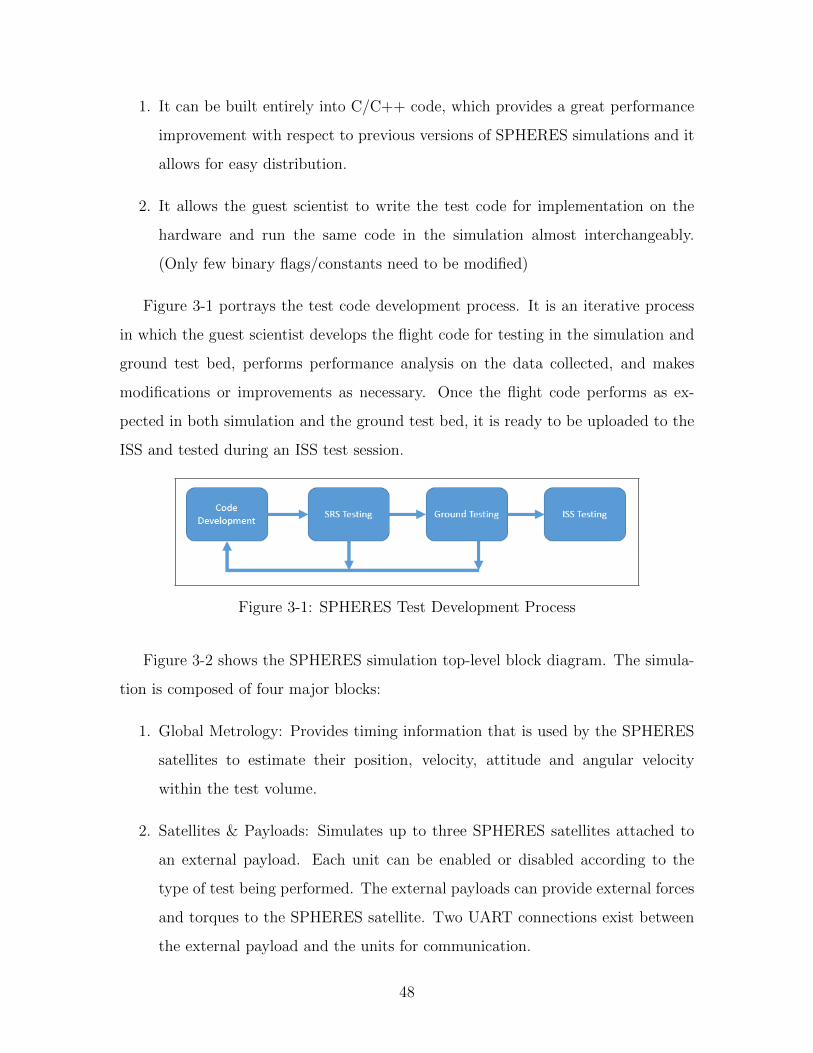
Figure 3-1 portrays the test code development process. It is an iterative process
in which the guest scientist develops the flight code for testing in the simulation and
ground test bed, performs performance analysis on the data collected, and makes
modifications or improvements as necessary. Once the flight code performs as ex-
pected in both simulation and the ground test bed, it is ready to be uploaded to the
ISS and tested during an ISS test session.
Figure 3-1: SPHERES Test Development Process
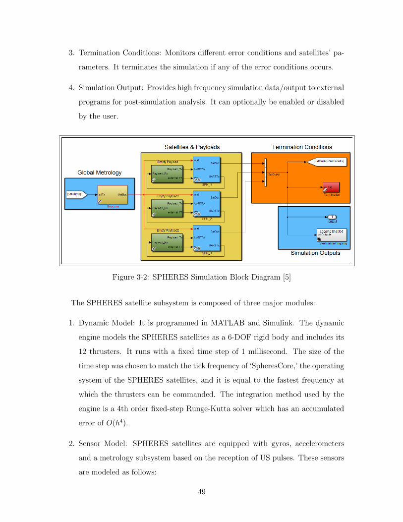
Figure 3-2 shows the SPHERES simulation top-level block diagram. The simula-
tion is composed of four major blocks:
1. Global Metrology: Provides timing information that is used by the SPHERES
satellites to estimate their position, velocity, attitude and angular velocity
within the test volume.
2. Satellites & Payloads: Simulates up to three SPHERES satellites attached to
an external payload. Each unit can be enabled or disabled according to the
type of test being performed. The external payloads can provide external forces
and torques to the SPHERES satellite. Two UART connections exist between
the external payload and the units for communication.
48
Page 51
3. Termination Conditions: Monitors different error conditions and satellites’ pa-
rameters. It terminates the simulation if any of the error conditions occurs.
4. Simulation Output: Provides high frequency simulation data/output to external
programs for post-simulation analysis. It can optionally be enabled or disabled
by the user.
Figure 3-2: SPHERES Simulation Block Diagram [5]
The SPHERES satellite subsystem is composed of three major modules:
1. Dynamic Model: It is programmed in MATLAB and Simulink. The dynamic
engine models the SPHERES satellites as a 6-DOF rigid body and includes its
12 thrusters. It runs with a fixed time step of 1 millisecond. The size of the
time step was chosen to match the tick frequency of ‘SpheresCore,’ the operating
system of the SPHERES satellites, and it is equal to the fastest frequency at
which the thrusters can be commanded. The integration method used by the
engine is a 4th order fixed-step Runge-Kutta solver which has an accumulated
error of O(h4).
2. Sensor Model: SPHERES satellites are equipped with gyros, accelerometers
and a metrology subsystem based on the reception of US pulses. These sensors
are modeled as follows:
49
Page 52
(a) Gyros: There are 3 gyros aligned with each of the body axes. The random
noise of the sensors is assumed to be zero-mean Gaussian noise and the
discretization error in the data acquisition is also captured.
(b) Accelerometers: The model takes into account the rotational coupling be-
tween acceleration and angular velocity due to the fact that the sensors
are not co-located with the CoM. The measurement noise has two com-
ponents: a zero-mean Gaussian noise and a high-variance random noise
that is caused by a ringing each time a thruster valve opens or closes.
This source exponentially decays after this event happens. In addition,
discretization error due to the Analog-to-Digital converter (ADC) is also
included in the measurement model.
(c) Ultrasound Global Metrology System (USGMS): It allows the SPHERES
satellite to compute an estimate of its current state. The state vector
includes position in the test volume, velocity, attitude and angular velocity.
The USGMS consists of a set of beacons (from 5 to 9 depending on the
configuration) that are placed in different corners of the test volume. Each
of the beacons possess a unique ID. An IR pulse emitted by the SPHERES
satellite triggers the beacons to send back an US pulse after certain amount
of time depending on their ID. The US receivers on the SPHERES satellites
detect these pulses, and using the Time of Flight (TOF) information, the
SPHERES satellites compute an estimate of their state. The noise model of
the USGMS includes random measurement losses, receiver and transmitter
biases, distance bias and random noise.
3. SPHERES Software Simulation: SPHERES satellites are equipped with a Texas
Instruments TMSC6701A Digital Signal Processor (DSP). For performance rea-
sons, a model of the operating system (OS) running on the DSP was created to
model the execution of the SPHERES software. The model implements basic
OS services such as threads, interrupts and synchronization constructs.
50
Page 53
3.3 Description and Integration of RINGS Simu-
lation
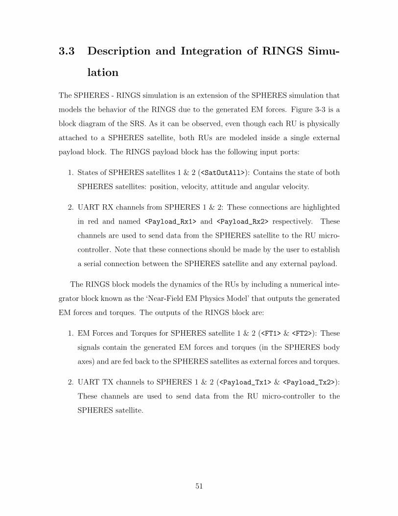
The SPHERES - RINGS simulation is an extension of the SPHERES simulation that
models the behavior of the RINGS due to the generated EM forces. Figure 3-3 is a
block diagram of the SRS. As it can be observed, even though each RU is physically
attached to a SPHERES satellite, both RUs are modeled inside a single external
payload block. The RINGS payload block has the following input ports:
1. States of SPHERES satellites 1 & 2 (<SatOutAll>): Contains the state of both
SPHERES satellites: position, velocity, attitude and angular velocity.
2. UART RX channels from SPHERES 1 & 2: These connections are highlighted
in red and named <Payload_Rx1> and <Payload_Rx2> respectively. These
channels are used to send data from the SPHERES satellite to the RU micro-
controller. Note that these connections should be made by the user to establish
a serial connection between the SPHERES satellite and any external payload.
The RINGS block models the dynamics of the RUs by including a numerical inte-
grator block known as the ‘Near-Field EM Physics Model’ that outputs the generated
EM forces and torques. The outputs of the RINGS block are:
1. EM Forces and Torques for SPHERES satellite 1 & 2 (<FT1> & <FT2>): These
signals contain the generated EM forces and torques (in the SPHERES body
axes) and are fed back to the SPHERES satellites as external forces and torques.
2. UART TX channels to SPHERES 1 & 2 (<Payload_Tx1> & <Payload_Tx2>):
These channels are used to send data from the RU micro-controller to the
SPHERES satellite.
51
Page 54
Figure 3-3: SRS Block Diagram
The reasoning behind using a single external payload block is that the ‘Near-Field
EM Physics Model’ block couples the state of the two RUs. An alternative design
could have been to model each RU as a separate block and place the ‘EM Physics
Model’ as an extra external block that incorporates the RUs’ state and the RUs’ coil
current as inputs. However, this design had a more complex signal interconnection
and did not render any advantage with respect to the current design.
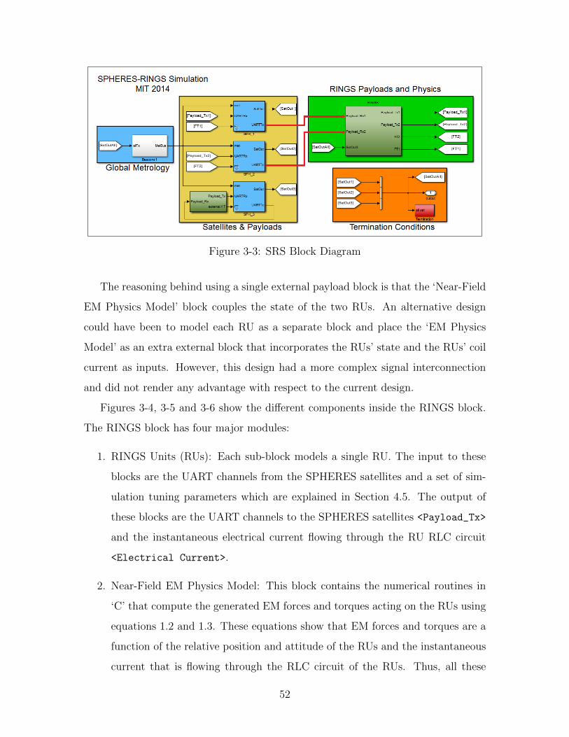
Figures 3-4, 3-5 and 3-6 show the different components inside the RINGS block.
The RINGS block has four major modules:
1. RINGS Units (RUs): Each sub-block models a single RU. The input to these
blocks are the UART channels from the SPHERES satellites and a set of sim-
ulation tuning parameters which are explained in Section 4.5. The output of
these blocks are the UART channels to the SPHERES satellites <Payload_Tx>
and the instantaneous electrical current flowing through the RU RLC circuit
<Electrical Current>.
2. Near-Field EM Physics Model: This block contains the numerical routines in
‘C’ that compute the generated EM forces and torques acting on the RUs using
equations 1.2 and 1.3. These equations show that EM forces and torques are a
function of the relative position and attitude of the RUs and the instantaneous
current that is flowing through the RLC circuit of the RUs. Thus, all these
52
Page 55
variables are inputs to this block. At each time step of the simulation, the
calculated forces and torques are fed back to the SPHERES satellites’ dynamic
engine (not shown in diagram). In addition, forces and torques in the inertial
frame are outputted but only used for analysis and debug purposes.
Figure 3-4: SRS Block Diagram - RINGS Units & EM Physics Model
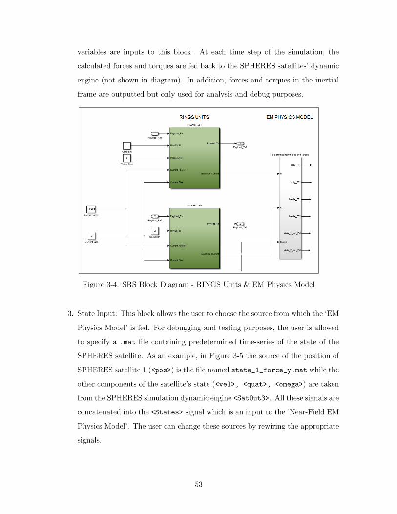
3. State Input: This block allows the user to choose the source from which the ‘EM
Physics Model’ is fed. For debugging and testing purposes, the user is allowed
to specify a .mat file containing predetermined time-series of the state of the
SPHERES satellite. As an example, in Figure 3-5 the source of the position of
SPHERES satellite 1 (<pos>) is the file named state_1_force_y.mat while the
other components of the satellite’s state (<vel>, <quat>, <omega>) are taken
from the SPHERES simulation dynamic engine <SatOut3>. All these signals are
concatenated into the <States> signal which is an input to the ‘Near-Field EM
Physics Model’. The user can change these sources by rewiring the appropriate
signals.
53
Page 56
Figure 3-5: SRS Block Diagram - State Input
4. Output Variables: As shown in Figure 3-6 simulation variables are saved in the
MATLAB workspace using ‘To Workspace’ Simulink blocks.
Figure 3-6: SRS Block Diagram - Output Variables
54
Page 57
Table 3.1 contains a description of the variables that are currently sent to the
MATLAB Workspace:
Variable Name Description
state_1 RU 1 State
state_2 RU 2 State
i_1 [A] RU 1 Instantaneous Current
i_2 [A] RU 2 Instantaneous Current
force_torque_body_1 Force & Torque on RU 1 in Body Frame
force_torque_body_2 Force & Torque on RU 2 in Body Frame
force_torque_inertial_1 Force & Torque on RU 1 in Inertial Frame
force_torque_inertial_2 Force & Torque on RU 2 in Inertial Frame
Table 3.1: SRS Output Variables
The following sections provide a description of the different sub-modules of the
SRS.
3.3.1 RINGS Units Firmware & SPHERES - RINGS Com-
munication
The firmware of the RUs was modeled using MATLAB functions executing at the same
frequency as in the RUs micro-controller. It receives commands from the SPHERES
satellites to set the configuration mode and the RMS current level flowing through
the RLC circuit. The SPHERES satellites are equipped with two UART ports that
can be used to communicate with external payloads. RUs use one of these serial
communication ports to receive commands from the SPHERES satellites and send
acknowledgement messages and telemetry data back. (See Appendix A for a descrip-
tion of the SPHERES - RINGS Interface and RINGS API)
The SPHERES simulation provides the two UART ports as an output signal of
the SPHERES satellite (<UARTTx>) and are connected to the payload as input ports.
Given that the RINGS firmware is modeled with MATLAB functions, it was necessary
55
Page 58
to create a mechanism to receive and to send bytes from the serial port, mimicking
the micro-controller’s UART module. Embedded in a MATLAB function a Receive
(RX) and a Transmit (TX) buffer were created along with read / write pointers for
each of them. Figure 3-7 shows how pointers are manipulated when a read and a
write operation occurs:
Figure 3-7: RINGS Communication Buffer
As an example, when byte ‘e’ is received, it is written into the RX buffer and the
tail pointer is moved forward. The MATLAB function executes periodically and reads
all the bytes pointing from the ‘head’ until the ‘tail’. Once the bytes are received,
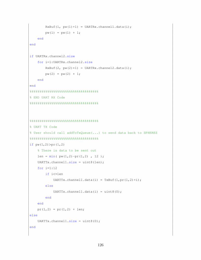
they are parsed into packets. Appendix B contains the source code of a MATLAB
function that can be used for any payload that communicates with the SPHERES
satellite through the UART channel. This function should be executed at a frequency
of 1kHz.
3.3.2 RINGS PI Current Controller
Initially, the current controller that was developed in Chapter 2 was intended to be
included as a sub-module in the RINGS block. However, this was not possible due
to the fact that the SPHERES - RINGS simulation runs at a fixed-size step of 1
56
Page 59
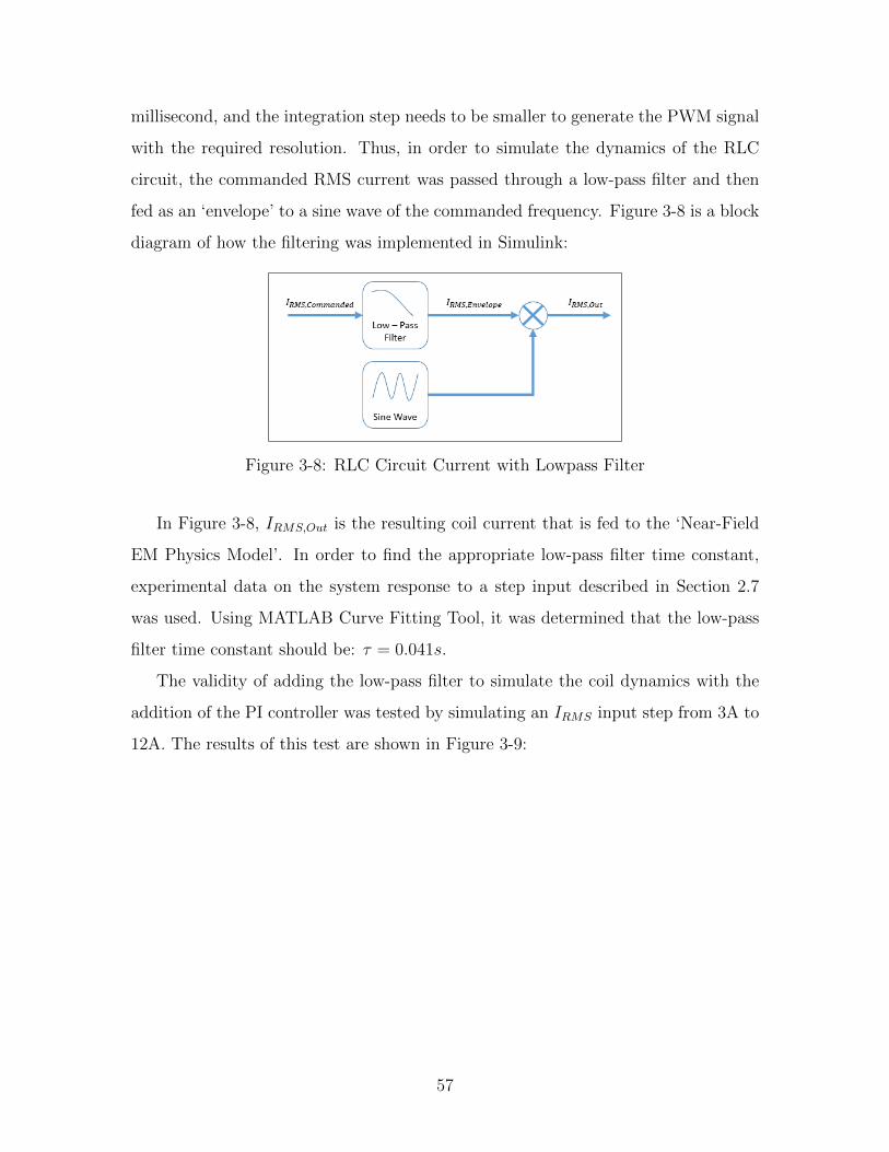
millisecond, and the integration step needs to be smaller to generate the PWM signal
with the required resolution. Thus, in order to simulate the dynamics of the RLC
circuit, the commanded RMS current was passed through a low-pass filter and then
fed as an ‘envelope’ to a sine wave of the commanded frequency. Figure 3-8 is a block
diagram of how the filtering was implemented in Simulink:
Figure 3-8: RLC Circuit Current with Lowpass Filter
In Figure 3-8, IRMS,Out is the resulting coil current that is fed to the ‘Near-Field
EM Physics Model’. In order to find the appropriate low-pass filter time constant,
experimental data on the system response to a step input described in Section 2.7
was used. Using MATLAB Curve Fitting Tool, it was determined that the low-pass
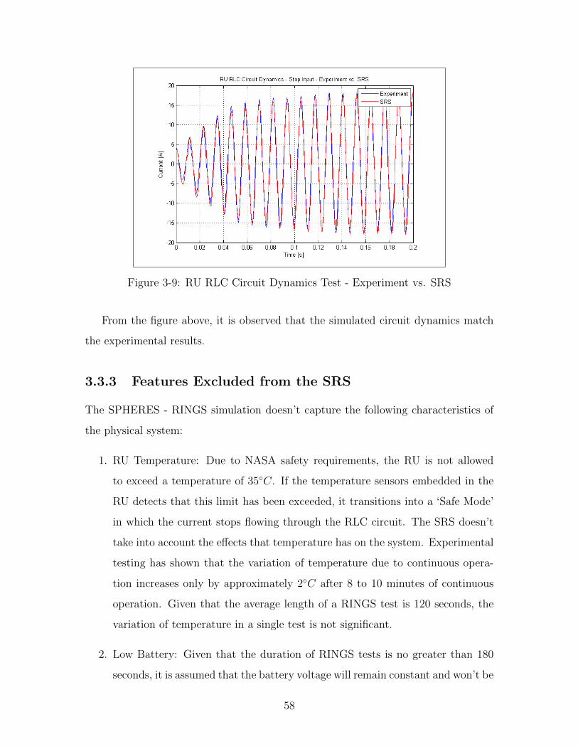
filter time constant should be: τ = 0.041s.
The validity of adding the low-pass filter to simulate the coil dynamics with the
addition of the PI controller was tested by simulating an IRMS input step from 3A to
12A. The results of this test are shown in Figure 3-9:
57
Page 60
Figure 3-9: RU RLC Circuit Dynamics Test - Experiment vs. SRS
From the figure above, it is observed that the simulated circuit dynamics match
the experimental results.
3.3.3 Features Excluded from the SRS
The SPHERES - RINGS simulation doesn’t capture the following characteristics of
the physical system:
1. RU Temperature: Due to NASA safety requirements, the RU is not allowed
to exceed a temperature of 35C. If the temperature sensors embedded in the
RU detects that this limit has been exceeded, it transitions into a ‘Safe Mode’
in which the current stops flowing through the RLC circuit. The SRS doesn’t
take into account the effects that temperature has on the system. Experimental
testing has shown that the variation of temperature due to continuous opera-
tion increases only by approximately 2C after 8 to 10 minutes of continuous
operation. Given that the average length of a RINGS test is 120 seconds, the
variation of temperature in a single test is not significant.
2. Low Battery: Given that the duration of RINGS tests is no greater than 180
seconds, it is assumed that the battery voltage will remain constant and won’t be
58
Page 61
lower than the threshold value. This assumption is valid given that experimental
data shows that the battery voltage remains constant for at least 8 minutes when
coil current levels are between 7A and 15A.
59
Page 63
Chapter 4
SPHERES - RINGS Simulation
(SRS) Validation
The RINGS program performed 4 sessions aboard the ISS between August 2013 and
July 2014. The first session objective was to perform a hardware checkout of the
RINGS to confirm its correct functionality. The objectives of the following three
sessions were to perform a mass identification of the system, and to perform open -
loop and closed - loop position control tests to support SRS validation.
4.1 SPHERES - RINGS Test Design
Two types of tests were designed to validate the SRS:
1. System Identification Tests (SIT): These tests are used to experimentally de-
termine the center of mass (CoM), inertia properties and thrusters force matrix
of each RU. The ‘Thrusters Tests’ consist of firing SPHERES thrusters sequen-
tially both individually and in pairs. The ‘Initial Positioning’ tests consist of
using thrusters to drive the RU to a target location in the test volume.
2. Electromagnetic Actuation Tests: These tests consist of performing maneuvers
using a pre-determined sequence of open-loop current commands. These tests
provide data about the EM actuation capability of the RUs in a microgravity
61
Page 64
environment. The tests have the following general architecture:
(a) Initial Positioning Phase: The RUs use the SPHERES thrusters to achieve
a target initial position and attitude. During this portion of the test the
RUs’ RLC circuits do not drive current.
(b) EM Actuation Phase: The RUs generate electromagnetic forces through
open-loop current commands.
(c) Data Download Phase: SPHERES & RINGS telemetry data recorded dur-
ing the test is transferred from the SPHERES satellites to the Express
Laptop Computer (ELC) controlled by the ISS crew.
In order to simplify the test setup of the RUs and to initially reduce the number
of variables needed to be accounted for, the position of one RU inside the test
volume was fixed using restraining tethers. Figure 4-1 is a diagram of the RUs
in one type of test performed in the ISS. The RU that is in the right side of the
picture is tethered to the Deck and Overhead walls of the ISS while the RU on
the left side is free-floating.
Figure 4-1: RINGS Test Initial Position Set-Up
As explained in Section 1.3.3, when the two RUs’ coil plane normal vectors are
co-axial and at a distance lower than 7 times their coil radius, the ‘Near-Field Model’
and ‘Far-Field Model’ start to diverge by more than 10% (see Figure 1-5). Given
62
Page 65
that the objective of the tests is to validate the ‘Near-Field Model’, the RINGS EM
actuation should be tested at distances lower than 2.1 meters (RU radius is 0.31m).
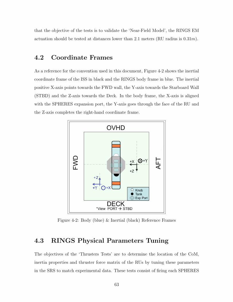
4.2 Coordinate Frames
As a reference for the convention used in this document, Figure 4-2 shows the inertial
coordinate frame of the ISS in black and the RINGS body frame in blue. The inertial
positive X-axis points towards the FWD wall, the Y-axis towards the Starboard Wall
(STBD) and the Z-axis towards the Deck. In the body frame, the X-axis is aligned
with the SPHERES expansion port, the Y-axis goes through the face of the RU and
the Z-axis completes the right-hand coordinate frame.
Figure 4-2: Body (blue) & Inertial (black) Reference Frames
4.3 RINGS Physical Parameters Tuning
The objectives of the ‘Thrusters Tests’ are to determine the location of the CoM,
inertia properties and thruster force matrix of the RUs by tuning these parameters
in the SRS to match experimental data. These tests consist of firing each SPHERES
63
Page 66
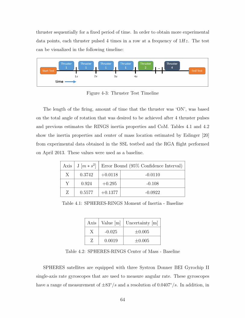
thruster sequentially for a fixed period of time. In order to obtain more experimental
data points, each thruster pulsed 4 times in a row at a frequency of 1Hz. The test
can be visualized in the following timeline:
Figure 4-3: Thruster Test Timeline
The length of the firing, amount of time that the thruster was ‘ON’, was based
on the total angle of rotation that was desired to be achieved after 4 thruster pulses
and previous estimates the RINGS inertia properties and CoM. Tables 4.1 and 4.2
show the inertia properties and center of mass location estimated by Eslinger [20]
from experimental data obtained in the SSL testbed and the RGA flight performed
on April 2013. These values were used as a baseline.
Axis J [m ∗ s2] Error Bound (95% Confidence Interval)
X 0.3742 +0.0118 -0.0110
Y 0.924 +0.295 -0.108
Z 0.5577 +0.1377 -0.0922
Table 4.1: SPHERES-RINGS Moment of Inertia - Baseline
Axis Value [m] Uncertainty [m]
X -0.025 ±0.005
Z 0.0019 ±0.005
Table 4.2: SPHERES-RINGS Center of Mass - Baseline
SPHERES satellites are equipped with three Systron Donner BEI Gyrochip II
single-axis rate gyroscopes that are used to measure angular rate. These gyroscopes
have a range of measurement of ±83/s and a resolution of 0.0407/s. In addition, in
64
Page 67
order to measure linear acceleration, SPHERES satellites have three Honeywell QA-
750 single-axis analog accelerometers. After the digital conversion is performed, these
sensors provide a resolution of 1.23 ∗ 10−4m/s2. It was desired for the RU to rotate
at least 5 degrees so that the motion could be observed by the ISS crew members.
Assuming that the CoM is at the geometric center of the SPHERES satellite:
τ = I ∗ α (4.1)
α = τ/IBaseline (4.2)
αx
αy
αz
=
0.025
0.010
0.017
rad/s2 (4.3)
Given the desired minimum angular rotation of 5 degrees, it was determined that
the lower bound for the total firing time needed to be at least 2.4 seconds. Since 4
firings occur per thruster, each firing period was set to 600ms. The SPHERES code
was implemented and tested in the SRS using the baseline moments of inertia listed
in Table 4.1.
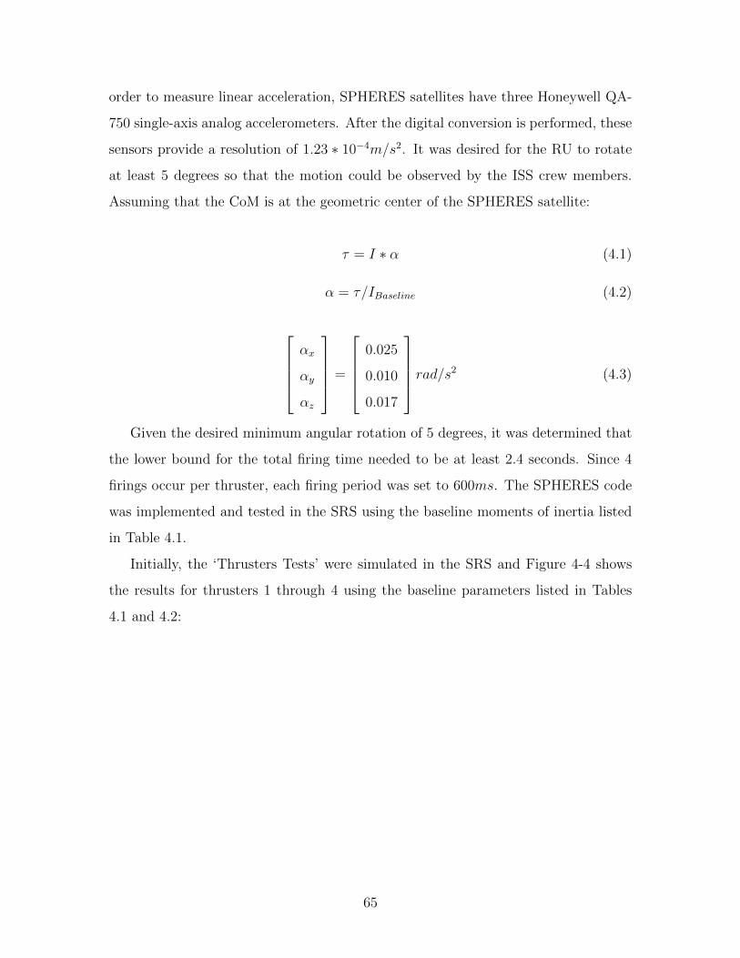
Initially, the ‘Thrusters Tests’ were simulated in the SRS and Figure 4-4 shows
the results for thrusters 1 through 4 using the baseline parameters listed in Tables
4.1 and 4.2:
65
Page 68
Figure 4-4: RINGS Unit Angular Velocity - SRS Results
As a reference, Table 4.3 shows the torque direction of the twelve SPHERES
thrusters:
Thruster Torque Direction Thruster Torque Direction
1 +Y 7 -Y
2 -Y 8 +Y
3 +Z 9 -Z
4 -Z 10 +Z
5 +X 11 -X
6 -X 12 +X
Table 4.3: SPHERES Thrusters Torque Direction
As it is expected, thrusters 1 and 2 produce a positive and negative angular
acceleration in the Y-axis respectively (see Table 4.3) while thrusters 3 and 4 act on
the Z-axis. The magnitude of the angular velocities observed in the Y-axis are lower
than in the Z-axis given the higher inertia in the first axis. These results show that
the RU will achieve angular velocities that will be within the range of measurements
of the sensors and distinguishable from the sensors noise.
66
Page 69
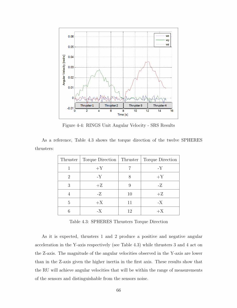
Subsequently, the ‘Thrusters Tests’ simulated in the SRS were performed in the
second RINGS ISS test session. The results are shown in Figure 4-5:
Figure 4-5: RINGS Unit Angular Velocity - ISS
The angular accelerations were estimated from the average slope of the angular
velocity. Firing thrusters multiple times was beneficial for data analysis since it
is observed that the recorded slopes have some variance associated with noise and
variability in the force provided by the SPHERES thrusters.
There are various differences between the predicted SRS results (Figure 4-4) and
the experimental data obtained from ISS (Figure 4-5). In the ISS test thrusters 1
and 2 (two of the four thrusters that exert a torque in the ±Y direction) produce a
much more reduced angular acceleration than the one predicted by the SRS. While
the SRS predicts a maximum angular velocity of 0.03rad/s, ISS results show that the
maximum angular velocity was only 0.004rad/s, one order of magnitude lower. This
reduction in thruster capability is due to the fact that the aforementioned thrusters
are impinged by the RINGS hardware. In addition, it can be observed that when
thrusters 1 and 2 are fired there is also a noticeable angular acceleration in the Z-axis
and the X-axis. This behavior can be attributed to the jet being deflected in the Z
and X directions after hitting the batteries or the RUs housing. Figure 4-6 shows
how thrusters 1 and 2 direct plume towards the batteries while thrusters 7 and 8 are
67
Page 70
blocked by the RU housing.
Figure 4-6: SPHERES-RINGS Thrusters Impingement
The thrusters impingement creates a higher uncertainty in the data recorded re-
sulting in broader confidence intervals for the inertia values. An accurate measure of
the inertia about the Y-axis is not as important as in the other two dimensions since
rotating the RU about the Y-axis doesn’t change the EM dynamics. However, the
reduced actuation capability may be of importance if translation using thrusters in
the X direction is required.
Combining the measurements from the gyros and accelerometers recorded during
the ISS thrusters tests, Hilton’s analysis [21], which is based on a least-square method,
determined that the RU tensor of inertia, CoM and thruster force matrix are:
Axis J [m ∗ s2]
X 0.3491
Y 0.7555
Z 0.4247
Table 4.4: SPHERES-RINGS Moment of Inertia - ISS
68
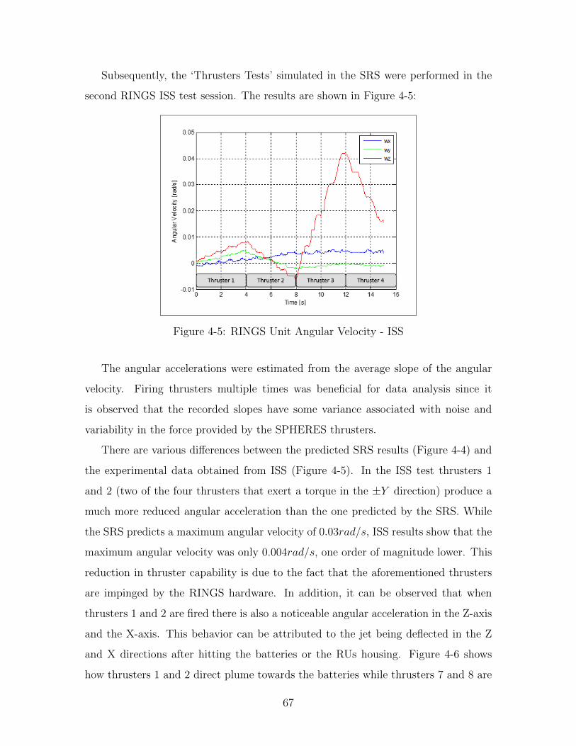
Page 71
Axis Position [m]
X -0.01245
Y 0.00633
Z 0.00160
Table 4.5: SPHERES-RINGS Center of Mass - ISS
Thruster Force X [N ] Force Y [N ] Force Z [N ]
1 0.011 -0.001 0.003
2 0.022 0.012 -0.004
3 0.013 0.104 0.000
4 0.005 0.077 0.001
5 -0.002 -0.008 0.077
6 -0.002 0.004 0.091
7 -0.008 -0.013 0.009
8 -0.012 -0.004 -0.003
9 0.008 -0.056 -0.004
10 -0.010 -0.066 0.002
11 0.002 0.017 -0.072
12 0.001 -0.023 -0.095
Table 4.6: SPHERES-RINGS Thrusters Force Matrix - ISS
The ‘Thruster Tests’ were again simulated using the new physical parameters
obtained by Hilton [21]. Figure 4-7 compares the gyro data recorded in the ISS with
the simulated results and Figure 4-8 compares Y-axis accelerometer data when one
of the thrusters is fired:
69
Page 72
Figure 4-7: Gyro Readings - ISS vs. SRS
Figure 4-8: Y-Axis Accelerometer Readings - ISS vs. SRS
The maximum percentage difference in angular velocities and linear accelerations
between the SRS and the ISS experiments is below 15%. The observed positive and
negative angular accelerations in the Z-axis (Figure 4-7) when thrusters 1 and 2 fire
70
Page 73
in the ISS are due to the thruster jet producing a torque when being deflected by
the battery packs (Figure 4-6). This phenomenon is not currently modeled in the
SRS due to the increased complexity and lack of data for validation. However, it is
considered that the effects on the control and simulation outputs are negligible.
4.4 RINGS Physical Parameters Validation
The second step in the validation process of the RINGS physical parameters is to
compare the SPHERES position and attitude recorded during the ‘Initial Positioning’
phase of the tests in the ISS with the SRS results.
As it is explained in Section 4.1, during this phase the RUs use only thrusters to
navigate to an initial target position and hold that position before they transition
to the ‘EM Actuation Phase’. A PD control law was used for position and attitude
control. This controller was employed under the assumption that the starting position
of RU (place at which the ISS crew member deploys the unit) would be near the
desired initial position and that the attitude error would also be small.
In order to choose the controller gains, the RU was modeled as a double-integrator
plant:
G =1
ms2(4.4)
The resulting gains and performance characteristics of the response are given in
tables 4.7 and 4.8 respectively:
71
Page 74
Position Controller Gains Value
Kp 0.15098
Kd 2.8418
Attitude Controller Gains Value
Kp,x 0.0028408
Kd,x 0.059696
Kp,y 0.0055598
Kd,y 0.11473
Kp,z 0.0042339
Kd,z 0.08897
Table 4.7: RINGS PD Controller Gains for Initial Positioning
Response Parameter Value
Overshoot 15.9%
Rise Time 8.15s
Settling Time 54.9s
Table 4.8: System Response Characteristics
The ‘Initial Positioning’ phase was simulated in the SRS and compared to the
results obtained in the ISS tests. In this particular test, the RU 1 (free-floating unit)
target position and attitude are:
72
Page 75
Target Position Value [m]
X +1m from RU 2 X-Position
Y 0.0
Z 0.0
Target Attitude Value [degrees]
Yaw -90
Pitch 0
Roll 180
Table 4.9: ‘Initial Positioning’ Phase - RU 1 Target Position and Attitude
Figures 4-9 and 4-10 show the results for position and attitude of RU 1 during the
‘Initial Positioning’ phase. In addition, Figure 4-11 shows the error in position and
attitude between the SRS and ISS tests.
Figure 4-9: RU 1 Position - ISS Test vs. SRS
73
Page 76
Figure 4-10: RU 1 Attitude - ISS Test vs. SRS
Figure 4-11: RU 1 Position and Attitude Error - ISS Test vs. SRS
During the ‘Initial Positioning’ phase, RU 1 (free-floating unit) is commanded to a
position one meter apart from RU 2 (tethered unit) in the X-axis. From the metrology
74
Page 77
system data received from ISS, it was determined that the RU 2 was tethered at
coordinates (−0.4m, 0m, 0m). Thus, as shown in Figure 4-9, RU 1 navigates to
coordinates (0.6m, 0m, 0m).
In Figure 4-11 it is shown that at the end of the ‘Initial Positioning’ phase (t = 60s)
the error in the X-axis is 2cm. This error is due to the fact that RU 2 is not rigidly
tethered and is still able to move up to 10cm in the X-axis (see Section 4.5). Thus,
the target X-position of RU 1 varies few centimeters as it receives the updated state
from RU 2. The errors in the Y-axis and Z-axis can be explained by the fact that the
actuation in the Y-direction was limited due to impingement and the coupling effect
on the thrusters.
In order to assess attitude error, quaternions are used to compute the quaternion
error relative to the desired attitude. Figure 4-11 shows the Euler angle rotations
in the SPHERES body frame that are derived from the error quaternions thereby
providing an intuitive understanding of attitude error. The quaternion values are
converted to ‘Euler Angles’ using a 321-rotation. These results show that the con-
troller attempts to correct for the error in all three axes and the final error is below
2.5 degrees. The source of these errors can be attributed to two main factors: (1)
the coupling effect of the thrusters that the RU controller does not account for and
(2) the presence of noise in the estimator. In other instances of equivalent tests, the
final error in the Z-axis is higher than 3 degrees due to the large amount of error
that the controller needs to correct. In order to mitigate this error, a more aggressive
controller would need to be designed that had a lower settling time. Given that the
‘EM Actuation Phase’ follows the ‘Initial Positioning’ phase, it is important that the
RU achieves the desired position and attitude during this phase. For the tests that
involved EM attraction, small errors in the RU attitude did not cause the system to
become unstable. Given the small differences observed between the ISS experimental
results and the SRS, it is determined that the ‘Initial Positioning’ phase in the SRS
is validated with a maximum error of 3cm for position and 3 degrees for attitude.
75
Page 78
4.5 EM Force Validation
‘Electromagnetic Actuation Tests’ focused on gathering data about the EM actuation
capability of the RUs in a microgravity environment. As it is described in Section
4.1, the RUs start by positioning themselves at a fixed distance from each other using
thrusters only. After the desired initial positioning is achieved, the ‘EM Actuation
Phase’ starts. For these tests, a predetermined current profile was used and is shown
in Figure 4-12. The shape, magnitude and phase of the current profile was driven by
the following factors:
1. EM actuation should produce a displacement of the RUs large enough to be
measured by the SPHERES estimator.
2. Current profile should prevent RUs from colliding with each other or make them
exit the test volume.
Figure 4-12: EM Actuation Test - Current Profile
Initially, this test was designed to validate both EM attraction and repulsion.
Thus, the current profile in Figure 4-12 drives the RUs current in-phase (attraction
force) for the first 20 seconds and 180 degrees out-of-phase (repulsion force) for the
last 15 seconds. However, for reasons explained in Section 4.6, the data gathered in
these tests could only be used to validate EM attraction.
76
Page 79
Given that closed-loop control with thrusters had not been demonstrated on ISS
for the RINGS hardware, three different types of tests were designed where thruster
actuation was responsible for a different number of DOF during the ‘EM Actuation
Phase’. Table 4.10 describes the actuation on all 6 DOF for each type of test:
Test Type X Translation Y Translation Z Translation X Rotation Y Rotation Z Rotation
1 EM None None None None None
2 EM Thrusters Thrusters Thrusters Thrusters Thrusters
3 EM None None Thrusters Thrusters Thrusters
Table 4.10: Thruster Actuation in 6 DOF
Translation in the X-direction is achieved by EM forces generated by the RINGS.
In type 1 tests, no thruster are fired during the ‘EM phase’. In type 2 tests, thrusters
are used to hold the axial configuration 1 in the 5 DOF so that the coils can more
effectively actuate in the axial direction. Type 3 tests were designed to assess the
actuation capability when the thrusters are only allowed to control torque. If the
thruster control proved ineffective during the ISS session, only Type 1 tests would
have been used for the rest of the session so that data on EM actuation could still
be gathered. Since it was observed that closed-loop thruster control was effective in
the ‘Initial Positioning’ phase, tests of type 2 and 3 were performed. These last two
types of tests could prove the feasibility of EMFF with coils and reaction wheels as
actuators.
As explained earlier, RU 2 is tethered to the Deck and Overhead of the ISS during
the tests. However, Figures 4-13 and 4-14 show that the RU is still able to move up
to 15cm in the X-direction and 25cm in the Z-direction from its initial position. In
addition, oscillations in attitude of up to 17 degrees are observed.
1Axial Configuration: The RUs’ coil plane normal vectors are co-axial (RUs are facing eachother)
77
Page 80
Figure 4-13: EM Actuation Test - RU 2 Position Oscillations
Figure 4-14: EM Actuation Test - RU 2 Attitude Oscillations
Due to these oscillations in position and attitude, modeling RU 2 as being fixed
at an initial position is not a valid assumption and it causes large discrepancies in
the computation of resulting EM forces and torques in the SRS. Thus, it was decided
78
Page 81
to validate the simulation by feeding the attitude of RU 1 and both position and
attitude of RU 2 from telemetry data obtained during the ISS test. All other state
variables of RU 1 are propagated and fed back to the SRS dynamics engine. Figure
4-15 shows a block diagram describing how inputs are fed into the SRS:
Figure 4-15: SRS Validation of Axial EM Tests - Inputs
Figures 4-16 plots the position of RU 1 during the ‘EM Phase’ of a type 1 test
predicted by the SRS and the telemetry data obtained from the ISS. In addition,
Figure 4-17 shows the error between these two variables.
Figure 4-16: Axial EM Type 1 Test - RU 1 Position - ISS Test vs. SRS
79
Page 82
Figure 4-17: Axial EM Type 1 Test - RU 1 Position Error - ISS Test vs. SRS
It is observed in Figure 4-17 that the error in the X-axis, where the strongest EM
force occurs, monotonically increases during the ‘EM Phase’ and it is unbounded.
The SRS results clearly diverge from the experimental ISS data: position error in
all three axis at the beginning of the ‘EM Phase’ (t = 0s) is less than 2cm and at
t = 28s, the error in the X-axis is approximately 1m. In Figure 4-16 there are three
major discrepancies between the SRS and the ISS test results:
1. During the ‘Attraction Phase’ (0s to 15s) the SRS underpredicts the EM force
that was observed during the ISS test causing RU 1 to move a lower distance.
2. During the ‘Repulsion Phase’ (15s to 28s) the SRS overestimates the repulsive
EM force. It is observed that while in the SRS RU 1 exhibits motion in the
negative X-axis, it is hardly noticeable in the ISS test.
3. RU 1 drifts in the positive Y and Z direction even though no thruster is fired
in this phase of the test. In addition, EM forces can’t produce this drift given
that data shows that the unit maintained its axial configuration with an error
of less than 15 degrees in all yaw, pitch and roll angles.
In order to explain and correct the observed discrepancies between SRS and ISS
experimental data, two major modifications were made to the SRS:
1. Drag Model: The SRS previously did not model drag forces that might be
present when operating in the ISS test volume. From data obtained in the ISS
80
Page 83
test session 51 for the SPHERES - VERTIGO program, Setterfield’s analysis
[22] concluded that the airflow inside the test volume in which the RINGS test
data was taken is at least 17.5 cm/s. Thus, the SRS was modified to incorporate
drag forces in both X, Y, and Z directions using the drag equation:
D =1
2ρ(VRINGS − VAirflow)2CDA (4.5)
The drag model uses a constant value for the velocity of the airflow. Table
4.11 lists the values used for the reference areas, airflow velocities and drag
coefficients, which are appropriate for the circular and rectangular shape of the
RUs with this Reynold’s number.
Parameter Value
ρ 1.225 kgm3
CD,x 1.28
CD,y 2.1
CD,z 2.1
VAirflow,x 16 cm/s
VAirflow,y 20 cm/s
VAirflow,z 11 cm/s
Ax 0.27m2
Ay 0.0576m2
Az 0.0576m2
Table 4.11: Drag Model Parameters
2. Current Model: The SRS was modified to allow for parameters related to the
RUs’ coil current to be tuned. The choice of the parameters was based on the
researchers evaluation that a possible cause of the discrepancies was a difference
between the current commanded to the RUs and the actual current that circu-
lated in the coils during the experiments. Section 4.6 provides a justification on
81
Page 84
why these modifications are valid. The following parameters were chosen:
(a) Current Offset: A constant variation of the current with respect to the
commanded RMS current.
(b) Linear Current Bias: A variation that is linearly proportional to the com-
manded RMS current.
(c) Phase Error: Difference between the commanded and the actual phase
shift between the current waves of the two RUs.
Through an iterative process, the values that provided the closest match between
SRS results and ISS data were found. These are shown in Table 4.12:
Parameter Value
Current Offset 0A
Linear Current Bias 1.0806
Phase Error (Attraction Phase) 0 deg
Phase Error (Repulsion Phase) 62 deg
Table 4.12: ‘Current Model’ Parameters
After tuning the parameters to obtain a close match with type 1 tests, type 2
and 3 tests were simulated using this modified version of the SRS which includes the
‘Drag Model’ acting on the RUs and the ‘Current Model’. The results of the RU 1
position and error for a type 3 test are shown in Figure 4-18 and 4-19 respectively:
82
Page 85
Figure 4-18: Axial EM Type 3 Test - RU 1 Position - ISS vs. SRS with ‘Drag Model’and ‘Current Model’
Figure 4-19: Axial EM Type 3 Test - RU 1 Error - ISS vs. SRS with ‘Drag Model’and ‘Current Model’
For the attraction portion of the test (t < 15s), the figures above show that the
modified SRS predicts the position of RU 1 with a maximum error of 4.2cm and 2cm
in the X & Y axes respectively. These errors represent 15% and 11% of the total
distance traveled. The telemetry data for the Z-position contains jumps which might
be caused by reflections of the US pulses with the RUs hardware. These reflections
83
Page 86
provide the SPHERES estimator erroneous TOF measurements and deteriorate its
accuracy. After t = 28s the system became unstable and the SRS results diverge from
the experimental data. Even though the error in the X-axis stays below 10cm for the
attraction portion of the test, it is observed that it monotonically increases. Thus,
at this point, it can only be stated that the modified SRS (simulation including drag
and current models) successfully models EM attraction maneuvers for a maximum
period of 20s.
The validation of the repulsion portion of the test was put on hold because a
phase error that affected repulsion and not attraction did not make sense from a
dynamics perspective. The following section discusses the RU hardware and software
verification process used in order to confirm that the system was operating correctly
before continuing with the dynamics model validation process.
4.6 RINGS Hardware/Software Verification
Section 4.5 describes the addition of a ‘Current Model’ to the SRS that increases the
commanded RMS current by a constant linear factor and introduces an additional
‘phase shift error’ only when the phase offset commanded is 180 degrees (repulsion
force). This section provides more insight into what caused each of those discrepancies
between the SRS and the experimental data.
A RINGS hardware verification was performed to fully characterize the shape of
the magnetic field generated by the RU coil. A test coil of 8.2cm diameter with 36
turns is co-axially centered with a RU coil and connected to an oscilloscope (on a
1MΩ/18 pF input) to measure the induced voltage on the test coil while the RU coil
drives current. In this experiment, the RU is commanded current levels from 1A to
12A at 1A steps and the induced voltage on the test coil is recorded. Figure 4-20
shows the induced voltage on test coil when the RU is commanded 3A RMS:
84
Page 87
Figure 4-20: RINGS Hardware Verification - Induced Voltage - 3A RMS
In Figure 4-20 it is observed that the wave contains what is commonly referred as
a ‘glitch’. This glitch can be described as an addition of an alternating pulse twice
the frequency of the sine wave to the sine wave itself. This anomaly is observed for all
the tested current levels. The ‘glitch’ has an alternating positive and negative value
in each cycle and always happens at the same time point of the cycle. As the current
level increases the duty cycle and magnitude of the glitch increase.
By taking the Fast Fourier Transform (FFT) of the recorded waves, it was deter-
mined that its fundamental frequency is around 83 Hz, which is the value expected
according to specifications. Figure 4-21 shows the FFT of the induced voltage when
the RU is commanded 3A RMS.
Figure 4-21: RINGS Hardware Verification - FFT - 3A RMS
By integrating the FFTs of the induced voltages at different RMS current levels,
85
Page 88
the additional power contained in the ‘glitched’ wave with respect to a perfect sinusoid
was determined. The results are shown in Table 4.13:
I RMS [A] Additional Power [%]
-12 2.86
-10 4.93
-7 9.00
-3 27.7
-1 39.9
1 38.1
3 25.3
7 9.61
10 5.28
12 3.61
Table 4.13: RINGS Hardware Verification - Additional Power
The shaded values are believed to be skewed due to the high noise in the acquired
waveforms. Given that the additional power proved to be significant it was decided
to connect an external Hall-Effect sensor2 and an oscilloscope in series with the RUs’
coils. This experiment provides a direct measure of the current that circulates through
the coils. Figure 4-22 is a diagram of the test set-up.
2Hall-Effect Sensor Part Number: ACS750 SCA-075 made by Allegro Microsystems.
86
Page 89
Figure 4-22: Hardware Verification Test Setup
The RUs are commanded RMS current levels from 1 to 10 A and the resulting
RMS current measured by the HES is recorded. Figure 4-23 shows the measured
RMS cuerrent as a function of the commanded RMS current:
Figure 4-23: Commanded vs. Real IRMS Current - Error: 8.6%
By using a linear regression, it is determined that the error between the com-
manded and the actual RMS current flowing through the coils is 8.6 %. This discrep-
ancy can be explained by the fact that the sampling rate of the HES in the RINGS
87
Page 90
is not high enough to capture the power added by the ‘glitch’ and thus the RINGS
current controller is fed back with an RMS value that is lower than the real one. The
difference between this error and the additional power that was used as a parameter
in the ‘Current Model’ of the SRS (8.06%, see Table 4.12) is 0.56%.
The second part of the RINGS hardware verification assesses the correct func-
tionality of the current synchronization mechanism between the two RUs. The tests
consist in commanding both RUs to different constant current levels (1A through
12A at 1A steps intervals both in 0 and 180 degrees phase shift). During these tests
the current waves are recorded using the same oscilloscope to measure their phase
difference.
When the RUs are commanded to be in-phase (0 degree shift), the RINGS behave
as expected and the current waves in the coils are permanently in-phase. However,
in the tests that command a 180 degree phase offset, it is observed that the current
waves randomly jump in and out of phase. The periods that the phase shift is 0 or
180 degrees are also random and it is not possible to discern any type of pattern.
Figure 4-24 is a snapshot of the current measurements during one of the 180 degrees
phase shift tests:
Figure 4-24: Hardware Verification - Phase Shift Anomaly
Initially, the two waves are 180 degrees out-of-phase as expected. However, at
88
Page 91
t = 0.24s (without giving any new command) they start transitioning to be in-
phase. After an analysis of possible causes of this anomaly, researchers identified a
memory allocation error in the RINGS firmware so it was modified to fix this erroneous
behavior.
Researchers conclude that RUs’ current waves alternating to be in and out of phase
is the cause of the ‘weaker’ repulsive force observed in the ISS data in comparison
to the one predicted by the SRS. By modifying the SRS to add an ‘average phase
error’ of 62 degrees during the ‘repulsion phase’, this weaker repulsive force could be
modeled to accurately match it to the force observed in the ISS test.
Since the firmware was modified to correct for the repulsion memory allocation
error, SRS validation tests for repulsion were completed in the following ISS test
session. The results of this validation are discussed in 4.7
4.7 EM Force Validation: Repulsion
After the hardware verification described in Section 4.6, a set of tests to validate ‘EM
repulsion’ were performed aboard the ISS. In the same manner as the ‘EM attraction’
tests, the RUs are initially in an axial configuration with an initial separation distance
of 0.8m in the X-axis. During the ‘EM Phase’ both RUs drive a constant RMS current
of 5A. The current waves have a phase shift of 180 degrees to produce the repulsive
EM force. Figure 4-25 compares the position results from the SRS and experimental
ISS data and figure 4-26 shows the error between them.
89
Page 92
Figure 4-25: Axial EM Repulsion Test - Position
Figure 4-26: Axial EM Repulsion Test - Error
The error in the X-axis, where the maximum EM repulsive force occurs, is less
than 1cm across the test. The error observed in the Y & Z axis are caused by the
fact that during the ‘Initial Positioning’ phase the SPHERES telemetry system was
not very accurate and as it can be seen in Figure 4-25 the RU didn’t start the ‘EM
Phase’ in the desired 0m position in the Y & Z axes. From the data gathered in this
test it is not possible to determine if the error in position are bounded since the error
in the Z-axis does not show to converge during the length of the test.
90
Page 93
4.8 EM Torque Validation
The objective of these tests is to gather data on the EM actuation capability in the
shear configuration. Similarly to the axial EM actuation tests, the RUs navigate to
their initial position using the SPHERES thrusters. Figure 4-27 shows the initial
configuration after the ‘Initial Positioning’ phase:
Figure 4-27: EM Shear Test - Initial Configuration
As it is shown in the previous figure, in the shear configuration RU 1 is rotated
90 degrees relative RU 2 about the Z-axis. In this configuration and due to the fact
that the two RUs are not perfectly aligned, a shear force and a torque are generated.
Given that both position and attitude of RU 1 change during the ‘EM Phase’,
only the position and attitude of RU 2 are fed from telemetry data obtained during
ISS tests. In these tests, the complete state of RU 1 is propagated and fed back to
the SRS dynamic engine. Figure 4-28 shows a block diagram describing how inputs
are fed into the SRS for the shear EM tests:
91
Page 94
Figure 4-28: SRS Validation of Shear Tests - Inputs
Figures 4-29 and 4-30 compare the position and attitude data of RU 1 during the
‘EM Phase’ predicted by SRS and the experimental ISS data:
Figure 4-29: Shear EM Test Type 1 - RU 1 Position - ISS vs. SRS
92
Page 95
Figure 4-30: Shear EM Test Type 1 - RU 1 Attitude - ISS vs. SRS
The attitude quaternions were converted to ‘Euler Angles’ using a 321-rotation. In
terms of Euler Angles, RU 1 starts with a 180-degree rotation in the X-axis meaning
that the SPHERES CO2 tank is facing the deck and the regulator knob is facing the
ISS Overhead. In the Z-direction, the unit starts with a negative 180-degree rotation
meaning that the SPHERES satellite expansion port is facing the AFT wall of the
ISS. The Y-rotation is 0 degrees meaning that there is no angular difference between
the inertial reference frame and the body reference frame.
In this configuration it is expected that the EM actuation would produce a torque
about the Z-axis and a force in the Y-axis. This is confirmed by the data of the test
shown in the figures above. Initially, RU 1 repelled from RU 2 and then attracted
when the rotation was around 90 degrees at approximately t = 10s. After time
t = 20s, when RU 1 second rotation occurs, the rotation about the X-axis was large
enough that the generated torque caused the system to become unstable.
Figure 4-31 shows the error for both position and attitude during the shear test.
There is a large discrepancy in the X & Z positions as well as in the roll angle. During
this test, an abnormal behavior was observed in the position and attitude estimation
93
Page 96
of RU 2: at t = 10s there is an instantaneous jump of 10cm and 10 degrees in the
estimate of RU 2. A possible explanation of the divergence of the results are the
inaccuracies in the state estimation of RU 2. However, the rotation about the Z-
axis predicted by the SRS, the major effect of EM actuation expected for this test,
matches the experimental ISS data with maximum error difference of 10 degrees.
Figure 4-31: Shear EM Test Type 1 - RU 1 Error - Validation
Given the small differences in the rotation about the Z-axis between the ISS test
and the SRS, it is considered that the SRS can successfully model tests in which shear
forces and torques occur with an error of 10 degrees.
4.9 Summary
This chapter steps through the SRS validation process through comparisons between
the results of tests performed in the ISS and the SRS. First, ISS and SRS results for
System Identification Tests are compared and values for CoM, inertia properties and
thrusters force matrix are determined. These tests assess the effects that the thruster
impingement have on the system. Subsequently, ‘Initial Positioning’ tests are used
to validate the new updated RINGS physical parameters. Afterwards, EM actuation
tests (Axial EM attraction, Axial EM repulsion and Shear EM tests) are compared
against the SRS. These tests revealed the need to account for the effect that drag
94
Page 97
forces have on the RUs. In addition, a verification of the RUs’ hardware and software
was necessary to explain discrepancies observed in the results.
The maximum position error in the EM attraction and repulsion tests is 10cm. In
the case of the EM shear test, the maximum errors in position and attitude are 15cm
and 30 degrees respectively. At this point, the researcher concludes that the SRS is
a tool that can be used to test control algorithms coded in the SPHERES satellites
with an accuracy in position and attitude of 15% for a maximum time period of 25s.
95
Page 99
Chapter 5
Evaluation of Closed-Loop Position
Controllers Using the SRS
5.1 Introduction
Using the latest version of the SRS, this chapter analyzes the performance of a
Proportional-Integral-Derivative (PID) controller for the position of the RUs when
they are in an axial configuration. Then, a direct adaptive control method known as
‘Input Shaping’ is incorporated to the PID controller in order to achieve stability of
the system.
Given the difficulties experienced while operating the RUs simultaneously aboard
the ISS, all the tests in this chapter model RU 2 as being at a fixed position inside the
testbed and driving a constant RMS current level. The closed-loop position control
tests start with the RUs placed in an axial configuration and can be classified by the
following variables:
1. RINGS initial orientation within the ISS testbed: there are two possible orien-
tations that may render optimal for the RINGS actuation capability. These are
described, simulated and compared in section 5.3.
2. Input type: ‘Station Keeping’ tests command RU 1 to keep the initial separation
distance and orientation constant. ‘Step Input’ tests command RU 1 to move
97
Page 100
to a target separation distance from RU 2 along the axial axis.
3. Attraction vs. Repulsion Step Input tests: In ‘Attraction’ tests, the RUs’ target
separation distance is lower than their initial separation distance. Contrarily,
in ‘Repulsion’ tests, the RUs’ target separation distance is greater than their
initial separation distance.
Table 5.1 describes the parameters of each type of test that is simulated and
described in this chapter:
Test Type Controller Type Testbed Configuration Input Type Initial Sep. [m] Target Sep. [m]
1 PID A Station Keeping 0.6 0.6
2 PID B Station Keeping 0.6 0.6
3 PID A Step 0.6 0.4
4 PID A Step 0.5 0.85
5 PID with Input Shaping A Step 0.5 0.85
Table 5.1: CLPC Test Parameters
5.2 Description of the CLPC
A PID controller is developed to demonstrate the capability of the RUs to achieve
position control in an axial configuration. The EM PID controller uses the RU’s coil
as the actuator to generate EM forces and achieve a target separation distance in the
axial axis. The standard SPHERES PID controls the other five DOF and maintains
the axial configuration using thrusters. Figure 5-1 is a block diagram of the PID
controller.
98
Page 101
Figure 5-1: PID Position Controller
In addition to the PID controller, an ‘EM axial mixer’ is implemented to convert
the desired force to a RMS current level. In order to create the mixer, the RMS
current level of RU 2 (IRMS,2) is first set to a constant value. Then, using the ‘Near-
Field EM Physics Model’ a function that outputs the desired RMS current for RU 1
as a function of desired EM axial force and separation distance can be obtained:
IRMS,Desired = f(FAxial,Desired, d)
The functions in Figure 5-2 plot the required RMS currrent in RU 1 to achieve 0.1N
(same force provided by SPHERES thrusters) as a function of the separation distance
when IRMS,2 is set to 7A (red) or 10A (blue). As an example, when IRMS,2 = 10A and
the RUs are at a distance of 85cm, an IRMS = 15A is required to achieve 0.1N of EM
force. If 0.2N is desired instead, these functions should be scaled by a factor of 2. The
black dashed line represents the maximum RMS current level that can flow through
the RU coil. These functions were approximated using a 7th-order polynomial and
implemented inside the SPHERES satellites’ controller algorithm.
99
Page 102
Figure 5-2: Mixer Function for Axial Configuration - IRMS/F vs. Axial SeparationDistance
The desired EM force that is output by the EM PID controller is fed into the EM
axial mixer along with the estimated separation distance between the RUs to obtain
the desired RMS current level for RU 1. At the end of each SPHERES control cycle,
this desired RMS current is sent from the SPHERES satellite to the RU.
5.3 Axial Station Keeping Tests for Optimal RU
Orientation
In Chapter 4, drag forces acting on the RUs were characterized assuming a constant
airflow in the test volume. Model calibration and the analysis performed by Setterfield
[22] determined that the maximum average air velocities occur in the Y & X directions
and their estimated average value are 20cm/s and 16cm/s respectively. In addition,
as it is explained in Section 4.3, there is thruster impingement in the four SPHERES
thrusters that are on the RUs’ X-Z plane. Given these two conditions, two possible
configurations could prove to be optimal to counteract the effects of the airflow for
axial configuration tests:
1. Configuration A (Figure 5-3): The SPHERES satellite CO2 tank points in the
positive Y-axis, while the expansion port points towards the positive Z-axis.
100
Page 103
In this configuration the impinged thrusters are oriented in the ±Z directions
which is where the airflow speed is the lowest (13cm/s).
Figure 5-3: Test - Configuration A
2. Configuration B (Figure 5-4): The SPHERES satellite CO2 tank points in the
positive Y-axis, while the expansion port points towards the positive X-axis. In
this configuration, the greatest frontal area of the RU faces the Z-axis where
the airflow speed is the lowest.
Figure 5-4: Test - Configuration B
Tests 1 & 2 (see Table 5.1) are simulated with the objective of assessing if the PID
controller is capable of performing a SK maneuver, where RU 1 maintains a constant
101
Page 104
separation distance from RU 2. In addition, tests 1 & 2 compare the performance
of the controller in keeping the RU at the desired separation distance for the two
possible configurations ‘A’ or ‘B’. Figures 5-5 and 5-6 show the position and attitude
errors, desired EM force and commanded IRMS,1 for tests 1 & 2 respectively. The
conventions used for these plots are:
1. The reference for both positions in the three axes and attitude is constant at 0.
2. Positive RMS current values correspond to RUs’ current being in-phase while
negative values correspond to a 180-degree phase offset.
Figure 5-5: PID Controller - Test 1 (Configuration A)
102
Page 105
Figure 5-6: PID Controller - Test 2 (Configuration B)
In both scenarios, the EM controller is able to keep RU 1 at a stable position
and the required RMS current levels are below the RINGS actuator’s saturation
point. In addition, the SPHERES controller successfully controls the position in the
remaining two axes and the RU attitude. Table 5.2 shows the maximum and RMS
errors for both position and attitude. It is observed that both controllers perform
better when the RUs are placed in configuration ‘A,’ than in ‘B’. The maximum
position error in configuration ‘B’ is double the error observed in configuration ‘A’
while the error in attitude is approximately three times larger. Also, the RMS error is
greater for configuration ‘B’. Given these results, it was decided that the ‘Step Input’
and ‘Input Shaping’ tests, which are described in the following sections, would be
simulated in configuration ‘A’. Using this configuration has the added advantage that
it is equivalent to the one already used for the ‘EM Actuation Tests’ during the ISS
tests described in Chapter 4. This gives the scientists confidence that configuration
‘A’ doesn’t have operational constraints that might prohibit performing these tests
103
Page 106
in future ISS test sessions.
Test Configuration A B
Position - Max. Abs. Error [m] 0.0437 0.0879
Position - RMS Error [m] 0.0199 0.0499
Attitude - Max Abs Error [deg] 6.5523 20.1574
Attitude - RMS Error [deg] 3.8283 10.6486
Table 5.2: PID Controller Performance Comparison - Configuration A vs. B
5.4 Step Input Tests
Test 3 places the RUs at an initial separation of 60cm and a step input of −20cm
(attraction) is commanded. The results of the test are shown in Figure 5-7:
Figure 5-7: PID Controller - Test 3 - Step Input - Attraction
As in the previous figures, subfigures (a) & (b) show the position and attitude
errors (reference is at 0) respectively. It is observed in subfigure (a) that the controller
104
Page 107
manages to move RU 1 to the commanded separation distance in the X-direction while
also maintaining the error in the Y & Z dimensions below 4cm. The response has
a rise time of 11.3 seconds, a percent overshoot of 20.8% and a settling time of 85
seconds. Subfigure (b) shows that the controller is also effective at keeping the desired
attitude within ±5 degrees. Finally, sub-figures (c) & (d) show that the desired EM
force has the same order of magnitude as the SPHERES satellites thrusters capability.
The required RMS current levels that are outputted by the EM mixer are below the
maximum current RMS levels that the RINGS is able to provide (marked by the black
dashed line) guaranteeing that the actuator is not being saturated during the test.
Test 4 is designed to assess the capability of the PID controller to drive the RUs
from an initial separation distance to a larger one. In this test, RUs are placed at
an initial separation distance of 50cm and given an step input of +35cm. Figure 5-8
shows the results of this test.
Figure 5-8: PID Controller - Test 4 - Step Input - Repulsion
Contrary to the previous test, the PID controller fails to drive RU 1 to the com-
manded separation distance and the system becomes unstable. In subfigure (b) it is
observed that the RU attitude error monotonically increases until t = 45s where the
105
Page 108
pitch error achieves a value of 60 degrees. These large errors in attitude make the
designed axial EM PID controller ineffective due to the coupling that exists between
the RU state and the generated EM forces and torques. Note that: (1) the EM force
that is desired in the axial direction is not achieved since the RUs are not in an
axial configuration, (2) EM torques and non-axial EM forces are generated that the
thrusters need to counteract to maintain the RUs axial configuration. It is observed
in subfigure (d) that at t = 14.5s the RU actuator is saturated and is not able to
provide the commanded force.
5.5 Direct Adaptive Control
Due to the instability observed in Test 4, a more robust control method known as
‘Input Shaping’ or ‘Model Referencing’ [23] was implemented. The commanded po-
sition and attitude are fed into a reference model that is designed to produce an
output with the desired response characteristics, such as settling time, rise time and
overshoot. Given that the controller tracks the output of reference model instead of
directly the step input, this method yields a much smaller tracking error and is less
likely to saturate the actuators. Figure 5-9 1 shows a block diagram of the EM PID
controller using ‘Input Shaping’.
Figure 5-9: EM PID Controller with ‘Input Shaping’
In Figure 5-9: dAxial,c is the commanded separation distance, dAxial,m is the sepa-
1Some blocks have been omitted for simplification.
106
Page 109
ration distance outputted by the reference model, ed,Axial is the distance error in the
axial axis and pAxial,1 and pAxial,2 are the estimated RUs’ positions in the axial axis.
Figure 5-10 shows the results of this test:
Figure 5-10: EM PID Controller - Input Shape - Repulsion
In this test the controller successfully drives the system to the commanded separa-
tion distance. The response has no overshoot, the rise time is 36.97s and the settling
time is 53.64s. Subfigures (c) & (d) show that the desired EM force has the same
order of magnitude as the SPHERES thrusters and the EM actuator is not saturated.
By using the ‘Input Shaping’ method it is possible to drive the RU to the desired
separation distance in an stable manner. However, it is observed in subfigure (b) that
the error in the roll angle is increasing. Given that the simulation could not be run
for a longer period of time, at this point it is not possible to determine if the attitude
is stable.
5.6 Summary
This chapter uses the SRS as a platform to simulate and test the performance of a
closed-loop position controller that uses the RUs’ coils as the actuators for controlling
the separation distance in the axial axis and thrusters for the other five DOF. For
these tests, RU 2 is at a fixed position and is commanded a constant RMS current
107
Page 110
level. Simulation results show that a PID controller is stable for SK and attrac-
tion maneuvers. However, an adaptive control method known as ‘Input Shaping’ is
necessary to achieve stability for repulsion maneuvers. Further analysis needs to be
performed to determine if the attitude of the RU is stable for this type of maneuver.
108
Page 111
Chapter 6
Conclusions and Future Work
6.1 Conclusions
This thesis begins with an introduction, motivation and theoretical background of
EMFF. Subsequently, a high-level description of RINGS provides a framework for
the primary contributions of this work.
The initial contribution of this thesis is the development and modeling of a PI
current controller in Simulink. The implementation of this module in RINGS is
to control of the current that circulates through the RUs’ coils, which is directly
proportional to the generated EM forces and torques. The creation and validation of
the current controller model using experimental data allowed researchers to evaluate
the stability of this controller for the RINGS experimental test scenarios and find the
gains that met the performance requirements.
The second contribution of this work is the modeling of the RINGS as an extension
to the existing SPHERES simulation referred to as SRS. ‘EM Actuation’ open-loop
tests are validated by comparing their results to the ones obtained during the ISS test
sessions. The validation process required the tuning of the RUs’ physical parameters
(CoM, inertia properties and thrusters force matrix) as well as a revision of the
SRS to include the effects of drag forces acting on the units. In addition, a general
explanation of how to integrate new payloads to the SPHERES simulation and serial
communication system is given. The SRS can be used as a tool to test, debug and
109
Page 112
evaluate control algorithms for RINGS before being tested on the ground testbed or
the ISS.
Finally, this thesis develops a PID position controller for the case in which the
RUs are initially positioned in an axial configuration. This controller uses EM forces
to control the RUs’ separation distance in the axial axis and SPHERES thrusters for
the position in the two other axes and for attitude. After SRS results showed that the
PID controller is not stable for repulsion maneuvers, a direct adaptive control method
known as ‘Input Shaping’ was used to achieve system stability for this maneuver. In
summary, it is shown that controlling the axial separation distance between the RUs
using EM actuation is feasible.
6.2 Future Work
This thesis has developed a model of RINGS that includes the effect of drag forces
on the RUs. However, this model has a pair of limitations:
1. Drag Coefficients: The plane of the RU was modeled as a flat solid plate per-
pendicular to the flow (Cd = 1.28) while the other two planes as a smooth brick
(Cd = 2.1). However, the RUs are not solid as flow can go through them. Thus,
the numbers used for Cd could be revised by placing the RUs in a wind tunnel
and measuring the drag forces at the adequate Reynolds number or by using a
CFD tool to obtain more accurate values of Cd.
2. Constant Attitude: The model takes the frontal areas and drag coefficients in
the three axes as constant inputs. Effectively, the model assumes that the RUs’
attitude will remain constant throughout the test for the calculation of the drag
forces. However, as the attitude of the RU changes from its initial value, both
the frontal area as well as the Cd in all three axes will change making this
assumption invalid. For the axial configuration tests described in Chapter 5,
this assumption holds as long as the attitude deviation of the RU from the axial
configuration is small. However, for tests that involve changes in attitude this
110
Page 113
model should be generalized.
The current version of the SRS can only be run in ‘Simulink Mode’ meaning that
it has to be open in Simulink to execute. This mode of execution has the disadvantage
that it is not easily distributable and major efforts have to be done to set the host
architecture variables appropriately. The SPHERES simulation can be generated into
independent C/C++ source code which greatly improves performance and portabil-
ity. However, configuration and compatibility issues have prevented researchers from
being able to generate independent source code for the SRS. A follow-on work effort
could be to resolve these misconfigurations to be able to compile the SRS and make
it easily distributable.
In Section 5.5, a controller that uses an adaptive control approach known as
‘Input Shaping’ is implemented. This work leaves room for research on more complex
adaptive control algorithms such as using time varying gains.
In their theses, Buck [4] and Eslinger [20] developed controllers for RINGS based
on ‘Optimal Control’ and ‘Dynamic Programming’ methods respectively. Their work
include simulations of these controllers for scenarios that can be tested aboard the ISS.
However, these controllers were never migrated or tested in the SPHERES-RINGS
architecture. Thus, one principal area for further work is to implement these type
of controllers in the SPHERES satellites, use the SRS to analyze their performance
and, subsequently, test them in the ISS.
Currently, the RINGS software architecture is a ‘foreground/background’ (or su-
perloop) system. In this type of architecture there is a looping construct for the main
portion of the application and interrupts handle time-critical events. The main loop
runs when there are no active interrupts. However, given the size, complexity and
tight time-control that is required for RINGS, it is difficult to identify the interac-
tions between all the software modules. A prime candidate for further development
of RINGS is to migrate the firmware to a Real-Time Operating System (RTOS) ap-
proach. In this architecture, concurrent tasks communicate between themselves as
they are all simultaneously managed by a kernel. Using this architecture offers the
following advantages: (1) more efficient use the micro-controller resources, (2) easier
111
Page 114
characterization of application’s performance and (3) shorter debugging/testing time.
In addition, by using this architecture, a follow-on exploration could be to implement
control algorithms in the micro-controller itself instead of the SPHERES satellite.
Up to this point, it has been observed that the communication between the
SPHERES satellite and the RU is not completely reliable. Two major anomalies
have been observed:
1. RUs firmware does not receive commands sent by the SPHERES satellite. Mes-
sages to change Operation Mode or set a RMS current level (See Appendix A)
are occasionally lost. Possible causes of this issue are: (1) error in the interrupt
routine of the RU firmware that handles the reception/processing of packets
through the UART line, (2) error in the Expansion Port Version 2 (EXPV2)
firmware.
2. Telemetry Data is lost for some time intervals. It has been noted that in some
occasions, telemetry data is lost for some portions of the test. Possible causes
of this error are: (1) data is lost in the communication line between the RU
firmware and EXPV2, (2) data is lost when it is transferred from the SPHERES
satellite to the ELC computer.
As it was explained in Section 4.1, the last phase of the RINGS tests is to ‘Down-
load Telemetry Data’. Currently, researchers receive an ‘End of Test’ code that indi-
cates if any anomaly occurred during the test. Adapting the SPHERES GUI to parse
RINGS telemetry data in a real-time fashion would give researchers more information
about the test and would allow them to proceed appropriately during the ISS test
session.
112
Page 115
Bibliography
[1] University of Maryland. Final Report for RINGS Payload, NASA Contract
NNH11CC33C. Technical report, DARPA, College Park, MD, September 2013.
[2] D. Alinger. System Analysis and Design for the Resonant Inductive Near-Field
Generation System (RINGS). Master’s thesis, University of Maryland, Depart-
ment of Aerospace Engineering, 2013.
[3] S. A. Schweighart. Electromagnetic Formation Flight Dipole Solution Planning.
PhD thesis, Massachusetts Institute of Technology, Department of Aeronautics
and Astronautics, June 2005.
[4] A. J. Buck. Path Planning and Position Control and of an Underactuated Elec-
tromagnetic Formation Flight Satellite System in the Near Field. Master’s thesis,
Massachusetts Institute of Technology, Department of Aeronautics and Astro-
nautics, June 2013.
[5] J. G. Katz. Achieving Broad Access to Satellite Control Research with Zero
Robotics. PhD thesis, Massachusetts Institute of Technology, Department of
Aeronautics and Astronautics, June 2013.
[6] ESA. Darwin Mission, December 2014. Online www.esa.int/science/darwin.
[7] O. Brown and P. Eremenko. Fractionated Space Architectures: a vision for
responsive space. Technical report, Defence Advanced Research Projects Agency,
2006.
113
Page 116
[8] J. Everist, K. Mogharei, H. Suri, N. Ranasinghe, B. Khoschnevis, P. Will, and
W.-M. Shen. A system for in-space assembly. Procceedings of 2004 IEEE/RSJ
International Conference on Intelligent Robots and SystemsAIAA Spacecraft and
Rockets, 2004.
[9] NASA. Robotic Refueling Mission, December 2014. Online http://www.nasa.
gov/mission_pages/station/research/experiments/778.html.
[10] D. R. Coulter. Nasas terrestrial planet finder mission: the search for habit-
able planets . Earths: DARWIN/TPF and the Search for Extrasolar Terrestrial
Planets, 539:4754, 2003.
[11] T. Hashimoto, S.-i. Sakai, K. Ninomiya, K. Maeda, and T. Saitoh. Forma-
tion flight control using super-conducting magnets. International Symposium on
Formation Flying Missions and Technologies, Centre National dEtudes Spatiales,
Touluse Space Center, France, 2002.
[12] L. M. Elias. Dynamics of Multi-Body Space Interferometers Including Reac-
tion Wheel Gyroscopic Stiffening Effects. PhD thesis, Massachusetts Institute of
Technology, Department of Aeronautics and Astronautics, 2004.
[13] R. Wawrzaszek and M. Banaszkiewicz. Control and reconfiguration of satellite
formations by electromagnetic forces. Proceedings of 2nd Microwave & Radar
Week in Poland, STW-2006, January 2007.
[14] M. Neave and R. Sedwick. Dynamic and thermal control of an electromagnetic
formation flight testbed. Master’s thesis, Massachusetts Institute of Technology,
Department of Aeronautics and Astronautics, 2005.
[15] A. Sakaguchi. Micro-electromagnetic formation flight of satellite systems. Mas-
ter’s thesis, Massachusetts Institute of Technology, Department of Aeronautics
and Astronautics, 2007.
[16] D. Miller, A. Saenz-Otero, J. Wertz, A. Chen, G. Berkowski, C. Brodel, S.
Carlson, D. Carpenter, S. Chen, and S. Cheng et al. Spheres: a testbed for
114
Page 117
long duration satellite formation flying in micro-gravity conditions. Proceedings
of the AAS/AIAA Space Flight Mechanics Meeting, Clearwater, Florida, pages
167–179, January 2000.
[17] J. Enright, M. Hilstad, A. Saenz-Otero, and D. Miller. The spheres guest sci-
entist program: collaborative science on the ISS. Aerospace Conference, 2004.
Proceedings. IEEE, 1, January 2004.
[18] E. M. Kong, A. Saenz-Otero, S. Nolet, D. S. Berkovitz, D. W. Miller, and S. W.
Sell. Spheres as a formation flight algorithm development and validation testbed:
current progress and beyond. 2nd International Symposium on Formation Flying
Missions and Technologies, 1:14–16, 2004.
[19] G. F. Franklin, J. D. Powell, and A. Emami-Naeini. Feedback Control of Dynamic
Systems. Pearson Prentice Hall, New York, NY, 7th edition, 2014.
[20] G. Eslinger. Dynamic Programming Applied to Electromagnetic Satellite Ac-
tuation. Master’s thesis, Massachusetts Institute of Technology, Department of
Aeronautics and Astronautics, May 2013.
[21] B. Alvisio and A. R. Hilton. SPHERES 46th ISS Test Session Report. Technical
report, MIT Space Systems Laboratory, December 2014.
[22] T. Setterfield. SPHERES 51st ISS Test Session Report. Technical report, MIT
Space Systems Laboratory, January 2014.
[23] H. Kaufman, I. Barkana, and K. Sobel. Direct Adaptive Control Algorithms: The-
ory and Applications. Communications and Control Engineering Series. Springer,
New York, NY, 2nd edition, 1997.
[24] J. Merk. SPHERES Expansion Port v2 Interface Control Document. Aurora
Flight Sciences, Four Cambridge, 11th Floor Cambridge, MA 02142.
115
Page 119
Appendix A
RINGS - SPHERES
Communication Interface and API
This appendix describes the communication system between the SPHERES satellites
and the RUs. The first section of this appendix explains the communication interface
between the SPHERES satellites and the RUs: how to integrate a RINGS test to a
GSP project and a description of the packet structure. The second section explains
the SPHERES-RINGS API.
A.1 RINGS Communication Interface
Communication between the SPHERES satellites and the RUs happens through a
UART connection. The UART line uses the RS-232 standard and is operated at a
baud rate of 115.2kbps. The SPHERES satellites send commands to the Expansion
Port Version 2 (EXPV2) [24] which in turn forwards the commands to the RU.
A.1.1 Integration of RINGS to a SPHERES GSP Project
In order to develop a project that uses the RUs, it is necessary to follow these steps:
1. The RINGS API functions (described in section A.2) are declared in two header
files: ringsUtil.h and ringsComm.h. These header files should be included in
117
Page 120
any source file that uses the API such as gsp.c.
2. To initialize communication with the RU, the user should call ringsInit(...).
A natural place to call this function is in ringsInitProgram() in file gsp.c.
3. When calling ringsInit(...) the user should also provide a pointer to a
callback function to handle the messages (acknowledgment, error and telemetry
data) received from the RUs. A default callback function is already provided by
the RINGS API. This function does a minimal parsing and processing of the ac-
knowledgment type packets. The user can provide his/her own implementation
of the callback function if needed.
4. SPHERES-RINGS tests should call ringsStartTest() at the beginning of each
test. A natural place to call this function is in gspTestInit() in gsp.c. This
function should be called to ensure that the communication channel is in a valid
state at the beginning of the RINGS test.
5. RINGS received messages should be downloaded to the ELC computer before
the test is ended since they are not preserved across consecutive tests. It is rec-
ommended that the task of the last maneuver of any RINGS test is to download
data from the SPHERES satellite to the ELC computer for post-processing. As
it is explained in section A.2, RINGS received data is accessible through the
RINGS API.
6. SPHERES-RINGS tests should call ringsEndTest() instead of ctrlTestTerminate()
to terminate a RINGS test. A natural place to call this function is either after
the last maneuver or in gspEndTest() in file gsp.c. If this is not called at the
end of a test, the communication channel could be left in an invalid state.
A.1.2 RINGS Packet Structure
The RINGS packet structure consists of a header and the body of the packet of
varying length. The current version of the protocol does not contain a checksum,
118
Page 121
length of the packet body or CRC. The types of packets and their respective sizes are
constant.
The header of the packet is two byte long: the first byte is an ‘Initialization Byte’
equal to 0xFF and the second byte is the type of packet being sent or received. Figure
A-1 shows the structure of the SPHERES-RINGS packets:
Figure A-1: SPHERES-RINGS Packet Structure
A.1.3 Transmitted Messages
Mode Packet
This packet commands the RUs to transition to the desired ‘Operation Mode’ and
the frequency of operation. The byte fields of the packet are described in Table A.1:
Byte Size(bits) Field Type Description
0 1(8) Mode unsigned char This field is used to specify the ‘Operation Mode’ that
the RU should transition to. The following byte
constants are used:
0x01: IDLE
0x02: EMFF
0x03: WPT-RX
0x04: WPT-TX
1-4 4(32) Frequency (Hz) unsigned int This field specifies the frequency in Hz at which the RU
should drive the RLC circuit.
5-8 4(32) SPHERES Time Stamp unsigned int This field contains the local SPHERES time.
9 1(8) Send Long Telemetry Packet unsigned char This field specifies if the RU should send periodically
‘Long Telemetry Packets’ back to the SPHERES
satellite after transitioning to the commanded mode.
The following byte constants are used:
0x00: Don’t send.
0x01: Send.
Table A.1: Mode Packet Structure Details
119
Page 122
PWM Packet
This packet is used to command the RU to drive the coil at a constant PWM duty
cycle. The RU won’t apply the commanded duty cycle if its current ‘Operation Mode’
is IDLE. The byte fields of the packet are described in Table A.2:
Byte Size(bits) Field Type Description
0-1 2(16) Count Amplitude unsigned short This field specifies the PWM duty cycle. This field should
contain a number between 0 (0% DC) and 200(100% DC)
2 1(8) Phase unsigned char This field specifies the phase offset at which the RU should
drive the RLC circuit. (RU coil). The following byte
constants are used (All other values are invalid):
0d0: 0 deg Phase Offset
0d180: 180 deg Phase Offset.
3-6 4(32) SPHERES Time Stamp unsigned int This field contains the local SPHERES time.
Table A.2: PWM Packet Structure Details
RMS Current Packet
This packet is used to command the RU to drive the RLC circuit at a specified con-
stant RMS current level. The RU won’t apply the command if its current ‘Operation
Mode’ is IDLE. The RU will apply a maximum RMS current level of 15A if the RMS
level value specified in the packet is 15A or greater. The byte fields of the packet are
described in Table A.3:
Byte Size(bits) Field Type Description
0-3 4(32) Command ID unsigned int This field contains a unique ID packet to identify the
command. This ID is generated by the SPHERES satellite.
4-8 4(32) SPHERES Time Stamp unsigned int This field contains the local SPHERES time.
9 1(8) Controller Enable unsigned char Deprecated. Should always be set to a constant value 0x01.
10 - 13 32(4) RMS Current Level float This field specifies the RMS current level.
14 1(8) Phase unsigned char This field specifies the phase offset at which the RU should
drive the RLC circuit. The following byte constants are
used (All other values are invalid):
0d0: 0 deg Phase Offset.
0d180: 180 deg Phase Offset.
15 - 18 32(4) Proportional Gain float This field specifies the Proportional Gain used in the PI
current controller.
19 - 22 32(4) Derivative Gain float Deprecated. Should be set to 0x00.
23 - 26 32(4) Integral Gain float This field specifies the Integral Gain used in the PI current
controller.
Table A.3: RMS Current Packet Structure Details
120
Page 123
A.1.4 Received Messages
Short Telemetry Packet
This packet is sent from the RU to the SPHERES satellite at a fixed frequency of
3Hz. The data received in this packet can be used for real-time operations, health
monitoring of the RU and for post-processing of the data. The byte fields of the
packet are described in Table A.4:
Byte Size(bits) Field Type Description
0-3 4(32) SPHERES Time Stamp unsigned int This field contains the last SPHERES time stamp
that was received from the SPHERES satellite
4-5 8(16) RMS Current unsigned short This field contains RMS current measured by the
RMS Chip 2 in the RU. The value is given in
counts and can be converted to Amperes using the
conversion formula listed in Table A.8.
6-7 2(16) Load Power unsigned short This field contains the power that is being
generated by the RU. Note that this field is only
meaningful when the RU ‘Operation Mode’ is
WPT-RX. The value is given in counts and can be
converted to Amperes using the conversion formula
listed in Table A.8 and RLC circuit resistance.
8-9 2(16) Coil Temperature unsigned short This field contains the RU coil temperature
measured by the temperature sensor. The value is
given in counts and can be converted to
temperature units using Table A.8
10-11 2(16) Exit Air Temperature unsigned short This field contains the measured temperature by
the sensor located at the Exit Air Fans. (For a
detailed description of the sensors and its physical
location see [2]). The value is given in counts and
can be converted to temperature units using Table
A.8
12-13 2(16) Duty Cycle unsigned short This field contains the duty cycle being applied to
the RLC circuit. Note that this value is meaningful
only when a PWM command was issued and PI
current controller is disabled.
14-15 2(16) Short Telemetry Packet Count unsigned short This field contains the ‘Short Telemetry Packet’
sequential number that has been sent from the RU
to the SPHERES satellite since the last RU reset.
16-19 4(32) Time Elapsed unsigned int This field contains the time in milliseconds elapsed
since the last SPHERES time stamp received. (See
SPHERES Time Stamp field)
20-23 4(32) Reference RMS Current float This field contains the reference RMS current level
used by the PI current controller. Note that this
value is meaningful only when the current
controller is enabled.
24 1(8) Reference Phase unsigned char This field contains the Reference Phase Offset.
25 1(8) Not Used - -
Table A.4: Short Telemetry Packet Structure Details
121
Page 124
Long Telemetry Packet
This packet is sent from the RU to the SPHERE satellite at 30 times the operation
frequency only when the ‘Send Long Packet’ byte is set. (See Mode Configuration
Packet section A.1.3). The byte fields of the packet are described in Table A.5:
Byte Size(bits) Field Type Description
0-1 2(16) Long Telemetry Packet Count unsigned char This field contains the Long Telemetry Packet
sequential number that has been sent from the RU
to the SPHERES satellite since the RU last reset.
2-5 4(32) SPHERES Time Stamp unsigned int This field contains the local SPHERES time.
6-9 4(32) Time Elapsed unsigned int This field contains the time in milliseconds elapsed
since the last SPHERES time stamp received. (See
‘SPHERES Time Stamp’ field)
10-11 2(16) unused - -
12 - 191 90x 2(16) Instantaneous Current unsigned short These fields (90 samples) contain the current in the
RLC circuit measured by Hall-Effect sensor in
counts. (See Table A.8 for conversion formula)
Table A.5: Long Telemetry Packet Structure Details
Operation Mode Acknowledgment Packets
This packet is sent from the RU to the SPHERE satellite to acknowledge the valid
transition to the commanded ‘Operation Mode’. The byte fields of the packet are
described in Table A.6
Byte Size(bits) Field Type Description
0 1(8) Operation Mode unsigned char This field contains the new ‘Operation Mode’ that the RU
transitions to.
1-4 4(32) Operation Frequency (Hz) unsigned int This field specifies the frequency at which the RU should
drive the RLC circuit. (Not applicable when the RU
transitions to IDLE mode.)
Table A.6: Operation Mode Acknowledgment Packet Structure Details
A.1.5 Telemetry Data Conversion Tables
Tables A.7 and A.8 contain RUs sensor value gains, physical parameters and references
to convert received telemetry data to physical units.
122
Page 125
Element Units Value
BCS RU - HES 1 - 83Hz [mV/A] 48.74
BCS RU - HES 2 - 83Hz [mV/A] 49.44
BCS RU - HES 3 - 83Hz [mV/A] 51.35
BCS RU - HES 1 - 462Hz [mV/A] 49.76
BCS RU - HES 2 - 462Hz [mV/A] 50.51
BCS RU - HES 3 - 462Hz [mV/A] 52.34
CCS RU - HES 1 - 83Hz [mV/A] 48.98
CCS RU - HES 2 - 83Hz [mV/A] 49.43
CCS RU - HES 3 - 83Hz [mV/A] 51.34
CCS RU - HES 1 - 462Hz [mV/A] 49.28
CCS RU - HES 2 - 462Hz [mV/A] 49.62
CCS RU - HES 3 - 462Hz [mV/A] 51.63
Gray RU - HES 1 - 83Hz [mV/A] 49.11
Gray RU - HES 2 - 83Hz [mV/A] 49.63
Gray RU - HES 3 - 83Hz [mV/A] 51.15
Gray RU - HES 1 - 462Hz [mV/A] 49.37
Gray RU - HES 2 - 462Hz [mV/A] 50.17
Gray RU - HES 3 - 462Hz [mV/A] 51.46
Bronze RU - HES 1 - 83Hz [mV/A] 49.10
Bronze RU - HES 2 - 83Hz [mV/A] 50.30
Bronze RU - HES 3 - 83Hz [mV/A] 51.53
Bronze RU - HES 1 - 462Hz [mV/A] 49.58
Bronze RU - HES 2 - 462Hz [mV/A] 50.90
Bronze RU - HES 3 - 462Hz [mV/A] 51.96
RU RLC Resistance [Ω] 1.2
RU RLC Inductance [mH] 11.9
RU RLC Capacitance - EMFF [pF ] 310
Table A.7: RINGS Units Sensor Gains and Physical Parameters
Element Units Function
RMS Current A = ([counts] ∗ (3300/1024) ∗ (1/GainHESensor)
Coil & Exit Air Temperature C = (([counts] ∗ 3300/1024) − 500) ∗ 0.1
Duty Cycle % = [counts]/2
Table A.8: Telemetry Data Conversion Factors
A.2 SPHERES - RINGS API
The SPHERES - RINGS API is composed of 6 functions that are declared in dif-
ferent header files according to their logical functionality. These header files should
be included in any SPHERES-RINGS project source files that needs to call these
functions.
Header File ringsComm.h
Prototypes for the following functions can be found in the file ringsComm.h
123
Page 126
void ringsSetCurrent(...)
Sets the RMS current through the RLC circuit to the specified value.
1 float RMS current level in Amperes to be set. Negative values are interpreted as having a 180 degree phase offset. Note:
The absolute maximum value for this parameter is 15. Any value greater than 15 or less than -15 will be
interpreted as 15A and -15A respectively.
2 float Current Controller Proportional Gain.
3 float Current Controller Derivative Gain. Note: This value can be set to 0 given that most recent version of controller
only uses Proportional and Integral gains.
4 float Current Controller Integral Gain.
int ringsSetDC(...)
Sets the Duty Cycle of the RU’s RLC circuit.
1 unsigned char Duty Cycle. Note: The absolute maximum value for this parameter is 100. Returns zero for success, or error
‘-1’ if an illegal parameter is passed.
2 unsigned char Phase Offset. Logical Identifier: ZERO_PHASE or OUT_PHASE.
int ringsSetMode(...)
Sets the Operational Mode of the RU. Returns zero for success and ‘-1’ if an illegal parameter is passed
1 unsigned char Operation Mode. Logical Identifier: IDLE_MODE, EMFF_MODE, WPTTX_MODE, WPTRX_MODE
2 unsigned int The operational frequency at which the RLC should be driven. Note: Not applicable when transitioning to
IDLE Mode.
Header File ringsUtil.h
Prototypes for the following functions can be found in the file ringsUtil.h
void ringsInit(...)
Initializes the UART connection with the RU and sets internal state variables. This function must be called
once in function: void gspInitProgram() in file gsp.c
1 EXPv2_CFG_CBK Callback function that will be registered when Configuration data is received from the Expansion Port
Version 2. If null no function will be registered.
void ringsStartTest()
Sets internal state variables. This function must be called at the start of every RINGS test. It is recommended to call this
function in: void gspInitTest() in file gsp.c
void ringsEndTest()
Sets internal state variables. This function must be called at the end of every test. It is recommended to call this function after
the last maneuver and in: void gspEndTest() in file gsp.c
124
Page 127
Appendix B
SPHERES - RINGS Simulation -
Payload UART TX/RX MATLAB
Code
function [UARTTx] = Payload(UARTRx)
% INITIALIZATION INTERNAL VARIABLES
%%%%%%%%%%%%%%%%%%%%%%%%%%%%%%%%%%%
% UART RX Code
%%%%%%%%%%%%%%%%%%%%%%%%%%%%%%%%%%%
persistent RxBuf pw pr TxBuf;
if (isempty(RxBuf) | | isempty(TxBuf) | | isempty(pr) | | isempty(pw))
RxBuf = zeros(2,1e5,'uint8');
TxBuf = zeros(2,1e5,'uint8');
pw = [0,0;0,0]; % Rx/Tx read/write pointers
pr = [0,0;0,0]; % First column for Rx; Second Column for Tx
end
% COLLECT DATA INTO RxBuffer
if UARTRx.channel1.size
for i=1:UARTRx.channel1.size
125
Page 128
RxBuf(1, pw(1)+1) = UARTRx.channel1.data(i);
pw(1) = pw(1) + 1;
end
end
if UARTRx.channel2.size
for i=1:UARTRx.channel2.size
RxBuf(2, pw(2)+1) = UARTRx.channel2.data(i);
pw(2) = pw(2) + 1;
end
end
%%%%%%%%%%%%%%%%%%%%%%%%%%%%%%%%%%%
% END UART RX Code
%%%%%%%%%%%%%%%%%%%%%%%%%%%%%%%%%%%
%%%%%%%%%%%%%%%%%%%%%%%%%%%%%%%%%%%
% UART TX Code
% User should call addToTxQueue(...) to send data back to SPHERES
%%%%%%%%%%%%%%%%%%%%%%%%%%%%%%%%%%%
if pw(1,2)>pr(1,2)
% There is data to be sent out
len = min( pw(1,2)-pr(1,2) , 12 );
UARTTx.channel1.size = uint8(len);
for i=1:12
if i<=len
UARTTx.channel1.data(i) = TxBuf(1,pr(1,2)+i);
else
UARTTx.channel1.data(i) = uint8(0);
end
end
pr(1,2) = pr(1,2) + len;
else
UARTTx.channel1.size = uint8(0);
end
126
Page 129
if pw(2,2)>pr(2,2)
% There is data to be sent out
len = min( pw(2,2)-pr(2,2) , 12 );
UARTTx.channel2.size = uint8(len);
for i=1:12
if i<=len
UARTTx.channel2.data(i) = TxBuf(2,pr(2,2)+i);
else
UARTTx.channel2.data(i) = uint8(0);
end
end
pr(2,2) = pr(2,2) + len;
else
UARTTx.channel2.size = uint8(0);
end
function [TxBuf,pw] = addToTxQueue(chan,msg,TxBuf,pw)
len = length(uint8(msg));
TxBuf(chan,pw(chan,2)+1:pw(chan,2)+len) = uint8(msg);
pw(chan,2) = pw(chan,2) + len;
%%%%%%%%%%%%%%%%%%%%%%%%%%%%%%%%%%%
% END UART TX Code
%%%%%%%%%%%%%%%%%%%%%%%%%%%%%%%%%%%
127