Development and validation of comprehensive closed formulasDevelopment and validation of comprehensive closed formulasfor atmospheric delay and altimetry correction in ground-basedfor atmospheric delay and altimetry correction in ground-basedGNSS-RGNSS-RThis paper was downloaded from TechRxiv (https://www.techrxiv.org).

LICENSE

CC BY-NC-SA 4.0

SUBMISSION DATE / POSTED DATE

29-04-2021 / 01-05-2021

CITATION

Nikolaidou, Thalia; Santos, Marcelo; Williams, Simon; Geremia-Nievinski, Felipe (2021): Development andvalidation of comprehensive closed formulas for atmospheric delay and altimetry correction in ground-basedGNSS-R. TechRxiv. Preprint. https://doi.org/10.36227/techrxiv.14345153.v1

DOI

10.36227/techrxiv.14345153.v1

1

Abstract—Radio waves used in Global Navigation Satellite

System Reflectometry (GNSS-R) are subject to atmospheric

refraction, even for ground-based tracking stations in applications

such as coastal sea-level altimetry. Although atmospheric delays

are best investigated via ray-tracing, its modification for

reflections is not trivial. We have developed closed-form

expressions for atmospheric refraction in ground-based GNSS-R

and validated them against raytracing. We provide specific

expressions for the linear and angular components of the

atmospheric interferometric delay and corresponding altimetry

correction, parameterized in terms of refractivity and bending

angle. Assessment results showed excellent agreement for the

angular component and good for the linear one. About half of the

delay was found to originate above the receiving antenna at low

satellite elevation angles. We define the interferometric slant

factor used to map interferometric zenithal delays to individual

satellites. We also provide an equivalent correction for the

effective satellite elevation angle such that the refraction effect is

nullified. Lastly, we present the limiting conditions for negligible

atmospheric altimetry correction (sub-cm), over domain of

satellite elevation angle and reflector height. For example, for 5-

meter reflector height, observations below 20° elevation angle have

more than 1-centimeter atmospheric altimetry error.

Index Terms—GPS, GNSS, GNSS-R, reflectometry,

atmospheric delay, tropospheric delay, ray-tracing, radio wave

propagation.

I. INTRODUCTION

LOBAL Navigation Satellite System Reflectometry

(GNSS-R) has been widely applied for coastal sea level

altimetry from ground-based tracking stations [1], [2], [3].

Unfortunately, GNSS-R altimetry suffers from atmospheric

refraction [4]. Its linear and angular components induce,

respectively, speed retardation and direction bending on both

the direct and reflected rays. The consequence is an

interferometric propagation delay, between the two ray paths,

as compared to the idealization of propagation in vacuum. The

atmospheric delay yields an atmospheric altimetry bias defined

by the altimetry retrieval method employed. For example, for a

10-m reflector height, the bias exceeds 0.5 m for a satellite near

Manuscript received _____; revised __; accepted ___. TN acknowledges

funding from Mitacs. FGN acknowledges funding from CNPq (457530/2014-

6, 433099/2018-6) and Fapergs (26228.414.42497.26062017).

T. Nikolaidou and M. C. Santos are with Department of Geodesy and

Geomatics Engineering, University of New Brunswick, Fredericton, NB,

Canada (e-mail: thalia.nikolaidou@unb.ca, marcelo.santos@unb.ca).

the horizon [5] and is thus significant even for near-surface

configurations [6]. It increases exponentially with satellite

elevation angle and linearly with reflector height, i.e., distance

between the antenna and the surface.

Frequently in the literature, the atmospheric delay in GNSS-

R is simplified as “twice the delay experienced between the

specular point and the reception antenna” [6], [9]. This is based

on the assumption that the effect of the atmosphere above the

receiver cancels out, and only those effects due to the bottom

layer, between the surface and the receiver, affect the altimetric

range [10], [11]. However, atmospheric models developed for

direct or line-of-sight propagation, as used in GNSS

positioning, cannot compensate for the total atmospheric

refraction effect [12]. That is because angular refraction,

experienced by the incoming rays in the portion of the

atmosphere above the antenna, does not necessarily cancel out

when forming the interferometric atmospheric delay.

The most accurate modeling for the atmospheric delay in

GNSS-R is provided by the raytracing technique [7], [13] . In

its rigorous formulation, it requires solving a direct two-point

boundary value problem (BVP), involving transmitting satellite

and receiving antenna, followed by a three-point BVP,

involving additionally the reflecting surface [2][5]. We have

found that rigorous raytracing may be simplified with

rectilinear raytracing if each direct and reflected ray paths are

replaced by the respective refracted or apparent tangent

directions [12]. A detailed description of an interferometric

raytracing procedure is given in [5].

Although raytracing results are general and comprehensive,

they require software that is not always available for GNSS-R

researchers. Furthermore, most atmospheric raytracing

software used in space geodesy are designed for direct only ray

paths. Here, we develop and validate closed-form expressions

for the atmospheric delay and corresponding altimetry

correction for use in ground-based GNSS-R. They are

parameterized in terms of ancillary atmospheric information

(average layer refractivity and elevation bending angle) besides

the independent geometrical variables (reflector height and

satellite elevation angle). Refractivity and bending may be

modeled as functions over space (latitude, longitude, altitude)

S. D. P. Williams is with National Oceanography Centre, Liverpool, UK, (e-

mail: sdwil@noc.ac.uk).

F. Geremia-Nievinski is with Department of Geodesy, Institute of

Geosciences, Federal University of Rio Grande do Sul, Porto Alegre, Brazil (e-

mail: felipe.nievinski@ufrgs.br).

Development and validation of comprehensive

closed formulas for atmospheric delay and

altimetry correction in ground-based GNSS-R

T. Nikolaidou, Student Member, IEEE, M. C. Santos, S. D. P. Williams, and F. Geremia-Nievinski,

Member, IEEE

G

2

and time (year, day of year, time of day). We validate the

derived closed-form expressions by comparison to raytracing

results, both rigorous and rectilinear.

Besides the main results above, we also provide closed

formulas for derived quantities, such as the interferometric slant

factor, used to map interferometric zenithal delays to individual

satellites, and an elevation angle correction, such that the full

atmospheric refraction effect is nullified. Finally, we provide

the limiting conditions for significant atmospheric altimetry

correction, in terms of satellite elevation angle and reflector

height; in other words, we indicate the observation conditions

under which linear and angular atmospheric refraction is

negligible in ground-based GNSS-R.

II. BACKGROUND

For the sake of keeping this work more self-contained, in this

Background section we briefly recapitulate the essential

concepts of atmospheric refraction in GNSS-R; for details, the

reader is referred to [5].

A. Atmospheric Delay Formulation

The atmospheric delay 𝑑 = 𝐿 − 𝐷, is defined in terms of two

intrinsic radio propagation quantities: the vacuum distance,

𝐷 = ‖𝒓1 − 𝒓2‖ and the radio length, 𝐿 = ∫ 𝑛 𝑑𝑙𝒓2

𝒓1, where 𝑛 is

the index of refraction. The vector norm is evaluated given any

two points, such as transmitting satellite and receiving antenna,

involved in the direct vacuum distance, 𝐷𝑑 = ‖𝒓sat − 𝒓ant‖.

The integral is evaluated along the bent ray path, of

infinitesimal arc length 𝑑𝑙 [5].

Introducing further the curve range, 𝑅 = ∫ 1 𝑑𝑙𝒓2

𝒓1, allows the

definition of two classical atmospheric delay components,

𝑑 = (𝐿 − 𝑅) + (𝑅 − 𝐷) = 𝑑𝑎 + 𝑑𝑔 (1)

The first quantity on the right-hand side of eq.(1), 𝑑𝑎, is the

along-path atmospheric delay:

𝑑𝑎 = 𝐿 − 𝑅 = ∫ 𝑁 𝑑𝑙𝒓2

𝒓1

(2)

where 𝑁 = 𝑛 − 1 is the refractivity. The second quantity, 𝑑𝑔,

in the end of eq.(1), is the geometric atmospheric delay:

𝑑𝑔 = 𝑅 − 𝐷 (3)

The definitions above (eq.1-3) can be applied to either the direct

path, yielding 𝑑𝑑 = 𝐿𝑑 − 𝐷𝑑 = 𝑑𝑑𝑎 + 𝑑𝑑

𝑔, or to the reflection

path, , yielding 𝑑𝑟 = 𝐿𝑟 − 𝐷𝑟 = 𝑑𝑟𝑎 + 𝑑𝑟

𝑔. The latter involves

the refracted specular point on the surface 𝒓sfc′ (not to be

confused with the vacuum specular point, 𝒓sfc) [5].

Corresponding interferometric quantities result from the

difference between reflection and direct quantities, for

example: interferometric vacuum distance, 𝐷𝑖 = 𝐷𝑟 − 𝐷𝑑;

interferometric radio length, 𝐿𝑖 = 𝐿𝑟 − 𝐿𝑑; and interferometric

curve range: 𝑅𝑖 = 𝑅𝑟 − 𝑅𝑑. Hence, the interferometric

atmospheric delay follows from two equivalent formulations:

𝑑𝑖 = 𝑑𝑟 − 𝑑𝑑 = 𝐿𝑖 − 𝐷𝑖 (4)

This definition is extended to the interferometric delay

components, 𝑑𝑖 = 𝑑𝑖𝑎 + 𝑑𝑖

𝑔:

𝑑𝑖𝑎 = 𝑑𝑟

𝑎 − 𝑑𝑑𝑎 = 𝐿𝑖 − 𝑅𝑖 (5)

𝑑𝑖𝑔

= 𝑑𝑟𝑔

− 𝑑𝑑𝑔

= 𝑅𝑖 − 𝐷𝑖 (6)

B. Atmospheric Raytracing

The radio length normally is calculated numerically based on

rigorous raytracing. The bent raypath is determined by solving

the Eikonal equation [14]: 𝜕

𝜕𝑙(𝑛 �̂�) = 𝛁𝑛

(7)

where �̂� = 𝜕𝒓/𝜕𝑙 is the ray tangent direction (a unit vector), 𝒓

is the evolving ray vector position, 𝑙 is the incremental arc

length, and 𝛁𝑛 = 𝛁𝑁 is the spatial gradient of index of

refraction or of refractivity. A two-point BVP defines the direct

raypath between the satellite and antenna position vectors

(𝒓sat 𝒓ant); a three-point BVP defines the reflection, which

includes additionally the refracted reflection point

(𝒓sat, 𝒓ant, 𝒓sfc′ ) [5].

The direct satellite elevation angle bending 𝛿𝑒𝑑 = 𝑒𝑑′ − 𝑒 is

the difference between refracted and vacuum satellite elevation

angles. It can also be calculated as 𝛿𝑒𝑑 = acos(Δ�̂�sat′ ⋅ Δ�̂�sat),

in terms of the bent ray tangent direction at the receiving

antenna, Δ�̂�sat′ = (𝒓sat

′ − 𝒓ant) ‖𝒓sat′ − 𝒓ant‖⁄ , in comparison

to the geometric or vacuum satellite direction Δ�̂�sat =(𝒓sat − 𝒓ant) ‖𝒓sat − 𝒓ant‖⁄ . A similar reflection satellite

elevation bending 𝛿𝑒𝑟 can be defined at the refracted specular

point. Their difference 𝛿𝑒𝑖 = 𝛿𝑒𝑟 − 𝛿𝑒𝑑 is the interferometric

elevation bending, which may be negligible, provided the

reflector height is sufficiently small and the satellite elevation

is sufficiently large [5].

Under certain conditions, each direct and reflected bent ray

paths may be approximated by straight line segments at the

respective refracted or apparent tangent directions:

𝒓 = �̌� + 𝑠 ⋅ �̂� (8)

where �̌� is the initial ray position and 𝑠 is the incremental ray

distance [15]. This approach requires solving only the two-point

BVP, for direct rigorous raytracing, to obtain the elevation

bending. The three-point BVP may be avoided, being replaced

for a rectilinear reflection raytracing. Finally, the direct path is

retraced, also based on a rectilinear ray path, for consistency

[15]. A remarkable finding was that the combined rectilinear

interferometric delay has good accuracy, despite each direct and

reflected rectilinear delays having poor accuracy separately.

This model accounts for the bulk of angular refraction

(elevation bending) and for practically all linear refraction

(speed retardation). For further details, the reader is referred to

[15].

C. Zenithal/Slant Factorization

The zenith interferometric atmospheric delay is defined as:

𝑑𝑖𝑧 = 𝑑𝑟

𝑧 − 𝑑𝑑𝑧 = 2(𝑑sfc

𝑧 − 𝑑ant𝑧 )

𝑑𝑖𝑧 = 2 ∫ 𝑁 𝑑𝑙

𝒓ant

𝒓sfc𝑧

= 2 ∫ 𝑁 𝑑𝐻𝐻

0

(9)

The vector 𝒓sfc𝑧 refers to the surface position immediately under

the antenna. Now we can factor out the interferometric slant

factor:

𝑓𝑖 = 𝑑𝑖 𝑑𝑖𝑧⁄ (10)

which is responsible for mapping the zenith delay to a specific

satellite elevation angle. Analogous expressions exist for the

delay components, 𝑓𝑖𝑎 = 𝑑𝑖

𝑎 𝑑𝑖𝑧⁄ and 𝑓𝑖

𝑔= 𝑑𝑖

𝑔𝑑𝑖

𝑧⁄ [15].

3

D. Altimetry Retrieval

The altimetry retrieval technique employed by a particular

instrument will dictate the corresponding atmospheric altimetry

bias and correction. One definition follows from half the rate of

change of atmospheric delay with respect to the sine of the

elevation angle [5]:

Δ𝐻 = −0.5 ∂𝑑𝑖 ∂ sin 𝑒⁄ = −0.5 𝑑𝑖𝑧 ⋅ ∂𝑓 ∂ sin 𝑒⁄ (11)

Equivalently, it can be expressed as the product of zenith delay

and half the rate of change of the slant factor. The partial

derivatives may be evaluated numerically via finite differencing

given a series of delay values versus elevation angle. This

expression applies to many retrieval algorithms that utilize the

“phase stopping” approach [11], including interferometric

Doppler measurements [16] and multipath signal-to-noise ratio

(SNR) measurements [1].

For completeness, we mention the “phase anchoring”

altimetry approach [11], which requires ambiguity-fixed

carrier-phase observables [17], [18]. The corresponding

atmospheric altimetry correction follows simply from the

absolute ratio Δ𝐻 = −0.5 𝑑𝑖 sin 𝑒⁄ . Here we focus on the rate-

of-change formulation, eq.(11).

III. CLOSED-FORM EXPRESSIONS

We start highlighting the role of the bottom atmospheric

layer, between the receiving antenna and the reflecting surface.

The layer thickness equals the antenna height or reflector depth,

𝐻. It complements the portion of the atmosphere above the

antenna, responsible for the elevation bending 𝛿𝑒. Based on

these principles, we report the closed-form expressions,

denoted with an overhead tilde for distinction from the rigorous

results. They are provided first for the atmospheric delay

components and later for the corresponding slant factors and

altimetry corrections. We end this section complementing the

main formulas, for delay and for altimetry, with formulas for

uncertainty propagation and also for the elevation angle

correction.

A. Atmospheric Layering

The zenith interferometric delay can be rewritten as 𝑑𝑖𝑧 =

2𝐻𝑁ℓ, where the newly introduced quantity

𝑁ℓ = 0.5𝑑𝑖𝑧/𝐻 (12)

is the average layer refractivity. Assuming a thin atmospheric

layer, it can be approximated as 𝑁ℓ ≈ (𝑁sfc + 𝑁ant)/2, in terms

of the refractivity at the surface and at the antenna height, or

simply 𝑁ℓ ≈ 𝑁ant, for negligible 𝐻.

To further pave the way for the development of closed-form

expressions, we define the layer slant distance:

𝐷ℓ = 2‖𝒓sfc − 𝒓ant ‖ (13)

It is twice the slant distance from antenna to the surface specular

reflection point. Besides the vacuum version in eq.(13), a

refracted or apparent layer slant distance can also be defined

as 𝐷ℓ′ = 2‖𝒓sfc

′ − 𝒓ant ‖, based on the refracted reflection point,

𝒓sfc′ .

B. Interferometric Atmospheric Delay

While the general raytraced vacuum distances (ordinary 𝐷

eq.(13) and apparent 𝐷′) are evaluated based on their defining

vector norms, the specific closed-form quantities below will be

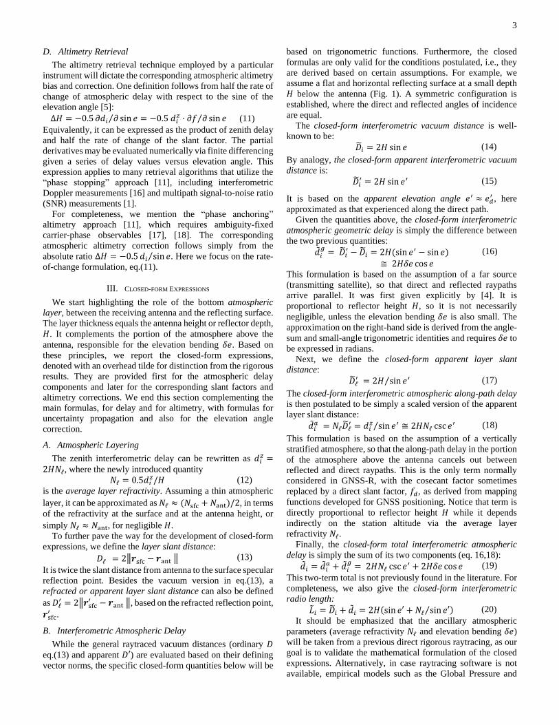
based on trigonometric functions. Furthermore, the closed

formulas are only valid for the conditions postulated, i.e., they

are derived based on certain assumptions. For example, we

assume a flat and horizontal reflecting surface at a small depth

𝐻 below the antenna (Fig. 1). A symmetric configuration is

established, where the direct and reflected angles of incidence

are equal.

The closed-form interferometric vacuum distance is well-

known to be:

�̃�𝑖 = 2𝐻 sin 𝑒 (14)

By analogy, the closed-form apparent interferometric vacuum

distance is:

�̃�𝑖′ = 2𝐻 sin 𝑒′ (15)

It is based on the apparent elevation angle 𝑒′ ≈ 𝑒𝑑′ , here

approximated as that experienced along the direct path.

Given the quantities above, the closed-form interferometric

atmospheric geometric delay is simply the difference between

the two previous quantities:

�̃�𝑖𝑔

= �̃�𝑖′ − �̃�𝑖 = 2𝐻(sin 𝑒′ − sin 𝑒)

≅ 2𝐻𝛿𝑒 cos 𝑒

(16)

This formulation is based on the assumption of a far source

(transmitting satellite), so that direct and reflected raypaths

arrive parallel. It was first given explicitly by [4]. It is

proportional to reflector height 𝐻, so it is not necessarily

negligible, unless the elevation bending 𝛿𝑒 is also small. The

approximation on the right-hand side is derived from the angle-

sum and small-angle trigonometric identities and requires 𝛿𝑒 to

be expressed in radians.

Next, we define the closed-form apparent layer slant

distance:

�̃�ℓ′ = 2𝐻 sin 𝑒′⁄ (17)

The closed-form interferometric atmospheric along-path delay

is then postulated to be simply a scaled version of the apparent

layer slant distance:

�̃�𝑖𝑎 = 𝑁ℓ�̃�ℓ

′ = 𝑑𝑖𝑧 sin 𝑒′⁄ ≅ 2𝐻𝑁ℓ csc 𝑒′ (18)

This formulation is based on the assumption of a vertically

stratified atmosphere, so that the along-path delay in the portion

of the atmosphere above the antenna cancels out between

reflected and direct raypaths. This is the only term normally

considered in GNSS-R, with the cosecant factor sometimes

replaced by a direct slant factor, 𝑓𝑑, as derived from mapping

functions developed for GNSS positioning. Notice that term is

directly proportional to reflector height 𝐻 while it depends

indirectly on the station altitude via the average layer

refractivity 𝑁ℓ.

Finally, the closed-form total interferometric atmospheric

delay is simply the sum of its two components (eq. 16,18):

�̃�𝑖 = �̃�𝑖𝑎 + �̃�𝑖

𝑔= 2𝐻𝑁ℓ csc 𝑒′ + 2𝐻𝛿𝑒 cos 𝑒 (19)

This two-term total is not previously found in the literature. For

completeness, we also give the closed-form interferometric

radio length:

�̃�𝑖 = �̃�𝑖 + �̃�𝑖 = 2𝐻(sin 𝑒′ + 𝑁ℓ sin 𝑒′⁄ ) (20)

It should be emphasized that the ancillary atmospheric

parameters (average refractivity 𝑁ℓ and elevation bending 𝛿𝑒)

will be taken from a previous direct rigorous raytracing, as our

goal is to validate the mathematical formulation of the closed

expressions. Alternatively, in case raytracing software is not

available, empirical models such as the Global Pressure and

4

Temperature (GPT) [19], [20] can be used to obtain the

refractivity at the station and models such as those of [21], [22]

can be used to approximate the elevation bending. In this case,

the discrepancy between closed formulas and raytracing will

include also errors in the atmospheric proxies (𝑁ℓ and 𝛿𝑒).

C. Interferometric Slant Factors

Slant factors cancel out the effect of zenith delay, isolating

the elevation angle dependency. For example, the closed-form

interferometric atmospheric along-path slant factor reads:

𝑓𝑖𝑎 =

�̃�𝑖𝑎

𝑑𝑖𝑧 =

1

sin 𝑒′= csc 𝑒′

(21)

Analogously, for the closed-form interferometric atmospheric

geometric slant factor we can write:

𝑓𝑖𝑔

=�̃�𝑖

𝑔

𝑑𝑖𝑧 =

sin 𝑒′ − sin 𝑒

𝑁ℓ≅

𝛿𝑒 cos 𝑒

𝑁ℓ

(22)

The expression for the closed-form interferometric total slant

factor is:

𝑓𝑖 = 𝑓𝑖𝑎 + 𝑓𝑖

𝑔= csc 𝑒′ + 𝛿𝑒 cos 𝑒 𝑁ℓ⁄

These trigonometric approximations will be compared to their

raytraced values, 𝑓𝑖, obtained independently following their

defining numerical ratios (eq.10).

D. Atmospheric Altimetry Correction

We provide the closed-form relative atmospheric altimetry

correction, normalized by reflector height 𝐻, to emphasize the

linear dependence on 𝐻. For rate-of-change altimetry retrievals,

we have:

Δ�̃�𝑖𝑎

𝐻=

𝑁ℓ

sin2 𝑒′(1 + 𝜉) ≈ 𝑁ℓ csc2 𝑒′ (23)

Δ�̃�𝑖𝑔

𝐻= −𝛿𝑒 tan 𝑒 (1 + 𝜉) + 𝜉 ≈ 𝜉 (24)

𝜉 = 𝜕𝛿𝑒 𝜕𝑒⁄ (25)

These expressions are not previously found in the literature. It

is evident the dependence on elevation bending 𝛿𝑒 (which must

be expressed in radians when used as multiplicative factor) as

well as its rate of change with respect to geometric elevation

angle, 𝜉. These trigonometric approximations will be compared

to their raytraced values, Δ𝐻𝑖 , obtained independently via

numerical derivative of delays as per eq.(11).

E. Altimetry Uncertainty Propagation

The closed-form atmospheric altimetry corrections (eq.23-

25) allow us to perform, for the first time, uncertainty

propagation on their input parameters:

𝜎𝛥�̃�𝑖𝑎 𝐻⁄ ≈ 𝜎𝑁ℓ

⋅ csc2 𝑒′ (26)

𝜎Δ�̃�𝑖𝑔

𝐻⁄ ≈ 𝜎𝜉 (27)

It is evident that the uncertainty in the atmospheric altimetry

correction due to that of refractivity, 𝜎𝑁ℓ, increases with

decreasing elevation angle in its along-path component, 𝛥�̃�𝑖𝑎.

On the other hand, the uncertainty in the geometric altimetry

component Δ𝐻𝑖𝑔

is driven essentially by that of the rate-of-

change of elevation bending with respect to the elevation angle,

𝜎𝜉. Applying a linear approximation, we find:

𝜉 = lim𝛥𝑒→0

𝛥𝛿𝑒

𝛥𝑒≈

𝛿𝑒2 − 𝛿𝑒1

𝑒2 − 𝑒1 (28)

𝜎𝜉 = 𝜎𝛿𝑒√2(1 − 𝜌𝛿𝑒)|𝛥𝑒|−1 (29)

Thus, 𝜎𝜉 is driven by the uncertainty of elevation bending 𝜎𝛿𝑒

(in radians), its autocorrelation 𝜌𝛿𝑒 (between -1 and +1), and the

elevation range Δ𝑒 under which 𝜉 is evaluated (e.g., 𝑒 ± 1°).

For the case of uncorrelated elevation bending noise (𝜌𝛿𝑒 = 0),

we find 𝜎𝜉 = 𝜎𝛿𝑒 |𝛥𝑒|⁄ . So, uncertainty propagation advises to

maximize the elevation angle range 𝛥𝑒 to minimize the

altimetry uncertainty, 𝜎Δ�̃�𝑖

.

F. Atmospheric Elevation Angle Correction

GNSS-R altimetry software may rely only on modifying the

input satellite elevation angle to compensate for atmospheric

refraction, with no possibility of using the total atmospheric

interferometric delay explicitly (eq.19). We thus define an

effective satellite elevation angle 𝑒∗ = 𝑒 + 𝛿𝑒∗ such that, when

input to the ordinary vacuum delay formula (eq.14), produces

the total radio length (eq.20):30

𝑒∗ ∶ 𝐷𝑖|𝑒∗ = 2𝐻 sin 𝑒∗ = 𝐿𝑖 (29)

Isolating the atmospheric elevation angle correction 𝛿𝑒∗ =𝑒∗ − 𝑒, we find:

𝛿𝑒∗ = asin(sin 𝑒′ + 𝑁ℓ sin 𝑒′⁄ ) − 𝑒 (30)

Applying the angle-sum and small-angle trigonometric

identities, it can be approximated by the sum of elevation

bending 𝛿𝑒 and a second-order elevation correction:

𝛿𝑒∗ = 𝛿𝑒 + 𝑁ℓ/(sin 𝑒 cos 𝑒) (31)

where the result is expressed in radians.

We provide the complete formula (eq.31) for the first time in

the literature. It should be noted that the usage of [6]

corresponds to the elevation bending only (𝛿𝑒∗ ≅ 𝛿𝑒), while

the usage of [23] seems equivalent to the second term only

(𝛿𝑒∗ ≅ 𝑁ℓ/(sin 𝑒 cos 𝑒)) of eq.(31).

IV. NUMERICAL RESULTS AND DISCUSSION

In the following, we assess closed-form expressions

developed above, by comparison to raytracing results. We start

with rectilinear raytracing then justify the discrepancies by

juxtaposing the rigorous raytracing results.

As atmospheric model, we used the CIRA climatology [24],

which neglects humidity. A single vertical profile is extracted

at zero latitude and longitude and used to structure a spherically

osculating atmosphere [25]. Geographical and temporal

variations are outside the scope of this work. The transmitter

satellite is at GNSS orbital altitude (~ 20,000 km). A fixed 10-

m reflector height is employed throughout, as a value

representative of ground-based GNSS-R stations.

For completeness, we also include an ad-hoc model

introduced in [9] and assessed by [4]:

�̃�𝑖∗ = 𝑑𝑖

𝑧 ⋅ 𝑓𝑑 (32)

where 𝑓𝑑 = 𝑑𝑑 𝑑𝑑𝑧⁄ is the direct slant factor, obtained from

rigorous direct raytracing. This model is motivated by the use

in GNSS-R of mapping functions developed for GNSS

positioning. The corresponding altimetry correction Δ�̃�𝑖∗ =

0.5 𝜕�̃�𝑖∗ 𝜕 sin 𝑒⁄ , is obtained via numerical differentiation. The

same numerical approach is used to obtain altimetry corrections

from the raytracing delay results.

A. Atmospheric Delay

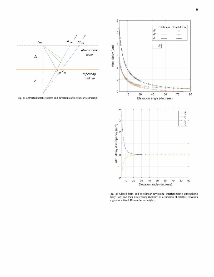
We observe in Fig. 2 (top) the overall excellent agreement

between closed-form total delay �̃�𝑖 and the respective

5

rectilinear raytracing result, whose discrepancy is shown in the

bottom panel of Fig. 2. For the atmospheric along-path delay

�̃�𝑖𝑎, the agreement is nearly exact at high elevations and it

remains at the millimeter level at low elevations, where the

discrepancy grows exponentially, reaching 3 mm or 7% near

the horizon. The atmospheric geometric delay, �̃�𝑖𝑔

has much

better agreement with raytracing results throughout the whole

elevation angle domain.

Although we have used the same elevation bending 𝛿𝑒 as

input for both closed formulas and rectilinear raytracing, the

agreements is not exact. To investigate the source of this small

disagreement, we have temporarily changed the raytracing

settings to force a more perfect matching with the assumptions

behind the closed formulas. More specifically, we have

increased the orbital altitude by 100x to put the transmitter more

distant and replaced the radial stratification for a plane-tangent

atmospheric structure. Although not realistic for GNSS-R

practice, such settings do improve the agreement of closed-

formulas to better than 0.01 mm (figure not shown). Therefore,

there is room for further improvements in the closed formulas

in the future.

The ad-hoc formulation, �̃�𝑖∗ (eq.32), follows closely the

rectilinear along-path results; their discrepancy, shown in Fig.

3 (bottom), is similar to that between �̃�𝑖𝑎 and the respective

rectilinear component, albeit with reversed sign and slightly

smaller magnitude. The discrepancy is larger between �̃�𝑖∗ and

the total rectilinear delay, reaching 5 cm at the lowest elevation

angle. Thus, the ad-hoc model based on direct raytracing and

similar mapping functions developed for GNSS positioning is

seen not to be an adequate replacement for the total

interferometric atmospheric delay.

Fig. S1 (in the supplementary material) recapitulates the

discrepancy in interferometric atmospheric delay between

rectilinear raytracing and rigorous raytracing, as checked

originally in [12]. The agreement in terms of total delay �̃�𝑖 and

its components is one order of magnitude smaller than that

shown in Fig. 2. That means it is safe to compare closed

formulas to rectilinear results as a surrogate for rigorous results.

B. Slant Factors

In Fig. 3 (top), the total slant factors (eq.10) and their

components are presented. There is excellent agreement

between closed-form and the respective rectilinear results,

whose discrepancy is shown in the bottom panel of the same

figure.

For the along-path slant factor, 𝑓𝑖𝑎, the agreement is nearly

exact at high elevations and it remains at the millimeter level at

low elevations for a 5 mm nominal interferometric zenith delay

(𝑑𝑖𝑧 = 5 mm ≈ 2 ⋅ 10 m ⋅ 250 ⋅ 10−6); near the horizon, the

discrepancy in 𝑓𝑖𝑎 grows exponentially, reaching 6.5%. The

atmospheric geometric slant factor, 𝑓𝑖𝑔

, has near exact

agreement with the rectilinear raytracing result, for all elevation

angles. For the total slant factor 𝑓𝑖 , its discrepancy is

dominated by that in 𝑓𝑖𝑎, as the discrepancy in 𝑓𝑖

𝑔 is negligible.

Finally, the direct slant factor, 𝑓𝑑 , follows closely the

rectilinear along-path result (Fig. 3, top). In Fig. 3 (bottom),

their discrepancy is similar to that of 𝑓𝑖𝑎, albeit with reversed

sign and slightly smaller magnitude. Thus, if 𝑓𝑑 were to be

used to compute the total delay, the error would reach almost

40 cm/m at the lowest elevation angle (Fig. 3, inset).

Fig. S2 highlights that interferometric along-path

atmospheric delay 𝑑𝑖𝑎, driven by the apparent layer slant

distance 𝐷ℓ (eq.18), is unrelated to the interferometric vacuum

distance 𝐷𝑖, whose self-difference drives the geometric

atmospheric delay 𝑑𝑖𝑔

(eq.16). With respect to the trigonometric

factors csc 𝑒′ and 𝛿𝑒 cos 𝑒 involved in, respectively, �̃�𝑖𝑎 and

�̃�𝑖𝑔

, it is interesting to see the similarity in their graphs (Fig. 3,

top), despite having very different formulas. It is also worth

noticing that although the trigonometric elements differ greatly

in order of magnitude, this is compensated to some extent by

the refractivity value (𝑁ℓ ≅ 0.00025). The ratio of the two

closed-form delay components reads:

�̃�𝑖𝑔

�̃�𝑖𝑎

=𝛿𝑒 cos 𝑒 sin 𝑒′

𝑁ℓ

It attains almost unity at 10-degree elevation (Fig. S2, left-hand

axis) where the two delay components are mostly balanced.

Also, for the conditions considered, �̃�𝑖𝑎 is always greater than

�̃�𝑖𝑔

.

C. Atmospheric Altimetry Correction

Now turning to the main result of interest, the atmospheric

altimetry correction (eq.23-24), we show it normalized by

reflector height, in units of centimeters per meter in Fig. 4 (top).

For example, for a satellite at 5° elevation angle, the total

relative atmospheric altimetry correction Δ�̃�𝑖 𝐻⁄ amounts to 4.5

cm/m, which scales to 45 cm altimetry correction for a reflector

height of 10 m; on the other hand, near zenith, the correction

amounts to 0.8 mm/m or 8 mm for a 10-m reflector height.

The inset in Fig. 4 (top) emphasizes that the geometric

altimetry correction component (eq.24) converges to a constant

value (0.5 mm/m) at zenith, despite the respective geometric

delay component (eq.16) converging to zero. This is explained

by the rate of change of elevation bending with respect to

elevation angle (eq.25).

The agreement between closed-form and rectilinear results

(Fig. 4, bottom) is good for the along-path altimetry component

Δ�̃�𝑖𝑎, whose discrepancy remains smaller than a tenth of the

correction. The agreement is excellent for the geometric

atmospheric altimetry correction, Δ�̃�𝑖𝑔

, whose discrepancy is

negligible for practical purposes. The closed-form total

atmospheric altimetry correction follows closely the raytracing

results; the corresponding discrepancy Δ�̃�𝑖 is dominated by

the discrepancy in the along-path component which remains

less than 5 mm/m even at the low elevation angles. The ad-hoc

model, Δ�̃�𝑖∗, agrees with the along-path term and misses the

geometric contribution.

The ratio of the respective altimetry correction components:

Δ�̃�𝑖𝑔

Δ�̃�𝑖𝑎

=𝜉

𝑁ℓ sin2 𝑒′⁄

is also shown in Fig. S3 (right-hand axis) and behaves in the

opposite way to the delay ratio. The geometric component is

larger than the along-path one for most of the elevation angle

domain. The ratio is balanced at 12° satellite elevation angle

due to the rate of change with respect to the elevation angle.

Near zenith, although the absolute altimetry correction is

minimal, the ratio approaches its maximum; at 85° satellite

6

elevation angle, the geometric altimetry correction is almost

twice the along-path one.

D. Cutoff Elevation Angle

We investigate the limiting conditions for negligible

atmospheric altimetry correction by showing in Fig. 5 its

contour lines over a bivariate domain of satellite elevation angle

and reflector height. The plot can be interpreted following

vertical or horizontal lines for either a fixed reflector height or

a fixed elevation angle.

For instance, when reflector height equals 1 m, a 13° cut-off

elevation angle corresponds to a negligible correction, of less

than 1 cm. If a greater reflector height is utilized, the cutoff

elevation angle grows almost linearly, e.g., it is 19° at a 2-m

reflector height and 30° at 5 m. For an antenna located an

altitude of 50 m above the reflecting surface, the altimetry

correction is at least 10 cm for any satellite observed above 30°

elevation angle; for that height, applying nothing but a tighter

elevation cut-off angle of 55° would reduce the altimetry error

to 5 cm.

From an orthogonal point of view, the same satellite would

produce an altimetry error proportional to the reflector height at

which is observed. For example, an error of nearly 0.1 cm and

10 cm correspond to a satellite at 30° elevation angle when

observed from antennas located at approximately 0.5 m and 50

m above the surface, respectively.

Fig. 5 (bottom) highlights the contour for 1-cm altimetry

correction and its components. It is apparent that heights greater

than 12.5 m need altimetry correction, even near zenith.

Conversely, at 5-degree elevation angle, even a few tens of cm

of height are enough to cause a significant altimetry correction.

E. Atmospheric Elevation Angle Correction

The atmospheric elevation correction 𝛿𝑒∗ (eq.30), resembles

twice the interferometric bending 𝛿𝑒 = 𝑒′ − 𝑒 yet offset by

approximately 50% throughout the elevation angle domain

(Fig. 6). Specifically, 𝛿𝑒∗ approaches 𝛿𝑒 the closest at 45°

elevation while it diverges at the edges i.e., at satellite elevation

angles of 5° and 85°, their difference is 0.16° and 0.18°

respectively. The atmospheric elevation correction is especially

pronounced near zenith, where it needs to account for the along-

path delay, in addition to the elevation bending.

V. CONCLUSIONS

In this study, we derived from first principles and validated

closed-form expressions for the interferometric atmospheric

delay, assuming a flat and horizontal reflecting surface at a

small depth below the receiving antenna. We also provided

closed-form atmospheric altimetry correction expressions,

necessary for unbiased GNSS-R sea-level retrievals.

Firstly, we described and formulated the intrinsic

propagation quantities based on two geometric quantities:

satellite elevation angle and reflector height. A greater insight

into the physics of the problem was given by considering the

atmospheric layer between antenna and surface. This revealed

that even small reflector heights are still subject to the

atmospheric refraction originating above the receiving antenna.

Next, the closed-form expression for the interferometric

along-path delay was given as a function of the layer slant

distance and the mean refractivity. The interferometric

geometric delay was computed as the difference between the

refracted and unrefracted interferometric distances. The

summation of the two yielded the total delay.

We then extended the delays’ definitions to the respective slant

factors by factoring out the zenith delay. The corresponding

atmospheric altimetry corrections were derived via analytical

formulas and approximations thereof. We gave a synopsis of

the uncertainty propagation in the atmospheric altimetry

correction. Finally, we presented the elevation correction that

can be utilized to account for the total atmospheric delay,

enabling easy adaptation in existing GNSS-R software.

We assessed the closed-form expressions against rigorous

and rectilinear raytracing results. The interferometric geometric

atmospheric delay exhibited excellent agreement, with

negligible discrepancies compared to raytracing. The

interferometric along-path atmospheric delay showed good

agreement to raytracing, with discrepancies due to the

refractivity approximation, that grew towards the horizon but

remained within few mm. Finally, an ad-hoc model based on

direct propagation proved insufficient to predict the total delay.

Slant factors showed similar performance to the delays

results and the discussion on their trigonometric elements

highlighted the similarity of the two components latter albeit

their differences in scale. The corresponding atmospheric

altimetry corrections were similarly derived and validated,

revealing a linear dependence on reflector height. Their

assessment against raytracing followed similar conclusions as

for the atmospheric delays.

We then presented the limiting conditions for neglecting any

atmospheric altimetry correction, in terms of a cutoff satellite

elevation for variable reflector height. For example, at a

reflector height of 1 m the cut-off elevation angle should be 13°

to keep the altimetry correction below 1 cm. The same 1-cm

altimetry correction would impose a cut-off elevation angle of

30° if observed from a 5-m reflector height. In any case, these

cutoffs can be surpassed with the application of the correction

expressions here developed.

It should be highlighted that the closed-form expressions

need no reflection raytracing, only line-of-sight raytracing so as

to obtain the elevation bending and mean refractivity as input.

Alternatively, existing tabulations and/or empirical models of

elevation bending and mean refractivity may be used by GNSS-

R users with no access to raytracing software.

Many neglected effects also to be considered in the future,

such as: atmospheric humidity (instead of just dry gases);

curvature of the Earth (spherical reflecting surface instead of a

tangent plane); geographical variations (station latitude,

longitude, altitude); temporal variations (time of day, day of

year, year-to-year); greater reflector height variations (thicker

atmospheric layer); and directional variations (satellite

azimuth). For further discussion of systematic and random error

sources, the reader is referred to Nikolaidou (2020).

7

References [1] K. M. Larson, R. D. Ray, F. G. Nievinski, and J. T. Freymueller, “The

Accidental Tide Gauge: A GPS Reflection Case Study From

Kachemak Bay, Alaska,” vol. 10, no. 5, pp. 1200–1204, Sep. 2013.

[2] K. M. Larson, R. D. Ray, S. D. P. Williams, K. M. Larson, R. D. Ray,

and S. D. P. Williams, “A 10-Year Comparison of Water Levels

Measured with a Geodetic GPS Receiver versus a Conventional Tide

Gauge,” J. Atmos. Ocean. Technol., vol. 34, no. 2, pp. 295–307, Feb.

2017.

[3] F. Geremia-Nievinski et al., “SNR-based GNSS reflectometry for

coastal sea-level altimetry – Results from the first IAG inter-

comparison campaign,” J. Geod., vol. 94, no. 8, p. 70, Aug. 2020.

[4] S. D. P. Williams and F. G. Nievinski, “Tropospheric delays in

ground-based GNSS multipath reflectometry-Experimental evidence

from coastal sites,” J. Geophys. Res. Solid Earth, vol. 122, no. 3, pp.

2310–2327, Mar. 2017.

[5] T. Nikolaidou, C. M. Santos, D. P. S. Williams, and F. Geremia-

Nievinski, “Raytracing atmospheric delays in ground-based GNSS

reflectometry,” J. Geod., vol. 94, no. 68, Aug. 2020.

[6] A. Santamaría-Gómez and C. Watson, “Remote leveling of tide

gauges using GNSS reflectometry: case study at Spring Bay,

Australia,” GPS Solut., vol. 21, no. 2, pp. 451–459, Apr. 2017.

[7] F. Fabra et al., “Phase altimetry with dual polarization GNSS-R over

sea ice,” IEEE Trans. Geosci. Remote Sens., vol. 50, no. 6, pp. 2112–

2121, Jun. 2012.

[8] S. Khajeh, A. A. Ardalan, H. Schuh, and H. S. S. Khajeh, A. A.

Ardalan, “Interferometric Path Models for GNSS Ground-Based

Phase Altimetry S.,” in The International Archives of the

Photogrammetry, Remote Sensing and Spatial Information Sciences,

2019, vol. XLII-4/W18, p. Volume XLII-4/W18, 2019.

[9] R. N. Treuhaft, S. T. Lowe, C. Zuffada, and Y. Chao, “2-cm GPS

altimetry over Crater Lake,” Geophys. Res. Lett., vol. 28, no. 23, pp.

4343–4346, Dec. 2001.

[10] E. Cardellach, F. Fabra, O. Nogués-Correig, S. Oliveras, S. Ribó, and

A. Rius, “GNSS-R ground-based and airborne campaigns for ocean,

land, ice, and snow techniques: Application to the GOLD-RTR data

sets,” Radio Sci., vol. 46, no. 5, pp. 1–16, Dec. 2011.

[11] V. U. Zavorotny, S. Gleason, E. Cardellach, and A. Camps, “Tutorial

on remote sensing using GNSS bistatic radar of opportunity,” IEEE

Geosci. Remote Sens. Mag., vol. 2, no. 4, pp. 8–45, Dec. 2014.

[12] T. Nikolaidou, M. C. Santos, S. D. P. Williams, and F. Geremia-

Nievinski, “A simplification of rigorous atmospheric raytracing

based on judicious rectilinear paths for near-surface GNSS

reflectometry,” Earth, Planets Sp., vol. 72, no. 91, Dec. 2020.

[13] V. Nafisi et al., “Comparison of Ray-Tracing Packages for

Troposphere Delays,” IEEE Trans. Geosci. Remote Sens., vol. 50, no.

2, pp. 469–481, Feb. 2012.

[14] M. Born and E. Wolf, Principles of optics Electromagnetic theory of

propagation, interference and diffraction of light, 7th expand.

Cambridge University Press, 1999.

[15] T. Nikolaidou, “Atmospheric Delay Modelling for Ground-based

GNSS Reflectometry (Ph.D. Dissertation),” University of New

Brunswick, 2020.

[16] A. M. Semmling et al., “On the retrieval of the specular reflection in

GNSS carrier observations for ocean altimetry,” Radio Sci., vol. 47,

no. 6, Dec. 2012.

[17] J. S. Löfgren, R. Haas, H.-G. Scherneck, and M. S. Bos, “Three

months of local sea level derived from reflected GNSS signals,”

Radio Sci., vol. 46, no. 6, Dec. 2011.

[18] M. Martin-Neira, P. Colmenarejo, G. Ruffini, and C. Serra,

“Altimetry precision of 1 cm over a pond using the wide-lane carrier

phase of GPS reflected signals,” Can. J. Remote Sens., vol. 28, no. 3,

pp. 394–403, 2002.

[19] K. Lagler, M. Schindelegger, J. Böhm, H. Krásná, and T. Nilsson,

“GPT2: Empirical slant delay model for radio space geodetic

techniques.,” Geophys. Res. Lett., vol. 40, no. 6, pp. 1069–1073, Mar.

2013.

[20] D. Landskron and J. Böhm, “VMF3/GPT3: refined discrete and

empirical troposphere mapping functions,” J. Geod., vol. 92, no. 4,

pp. 349–360, Apr. 2017.

[21] G. G. Bennett, “The Calculation of Astronomical Refraction in

Marine Navigation,” J. Navig., vol. 35, no. 02, p. 255, May 1982.

[22] T. Hobiger, R. Ichikawa, Y. Koyama, and T. Kondo, “Fast and

accurate ray-tracing algorithms for real-time space geodetic

applications using numerical weather models,” J. Geophys. Res.

Atmos., vol. 113, no. 20, pp. 1–14, Oct. 2008.

[23] D. J. Purnell, N. Gomez, N.-H. H. Chan, J. Strandberg, D. M.

Holland, and T. Hobiger, “Quantifying the Uncertainty in Ground-

Based GNSS-Reflectometry Sea Level Measurements,” IEEE J. Sel.

Top. Appl. Earth Obs. Remote Sens., 2020.

[24] E. L. Fleming, S. Chandra, J. J. Barnett, and M. Corney, “Zonal mean

temperature, pressure, zonal wind and geopotential height as

functions of latitude,” Adv. Sp. Res., vol. 10, no. 12, pp. 11–59, Jan.

1990.

[25] F. G. Nievinski and M. C. Santos, “Ray-tracing options to mitigate

the neutral atmosphere delay in GPS,” Geomatica, vol. 64, no. 2, pp.

191–207, 2010.

8

Thalia Nikolaidou received her Diploma

in Rural and Surveying Engineering from

Aristotle University of Thessaloniki

(AUTh), Greece. In 2020, she completed

her Ph.D. on tropospheric imprints on

GNSS Reflectometry and advanced

modelling of atypical atmospheric

conditions for GNSS applications. Her

research interests include the use of global

and regional Numerical Weather Models for

parametrization and precise prediction of the tropospheric

delay, modelling the asymmetry of the lower atmosphere

and Precise Point Positioning for GNSS-Meteorology. She

is associated with the UNB-Vienna Mapping Functions 1

Service (VMF1) and is part of the UNB’s GNSS Analysis

and Positioning Software (GAPS) developing team.

Marcelo C. Santos is a Professor at the

Department of Geodesy and Geomatics

Engineering at the University of New

Brunswick (UNB), Canada. He holds a M.

Sc. Degree in Geophysics from the

National Observatory, in Rio de Janeiro,

and a Ph.D. Degree in Geodesy from the

University of New Brunswick. His

research interest relates to geodetic

applications of global navigation satellite

system and to modelling of Earth’s gravity

field. His most recent contributions include a rigorous

definition of orthometric height, research on precise point

positioning (PPP), the development of the PPP research

platform GAPS, and investigation on the use of numerical

weather prediction models for modelling the neutral-

atmosphere, including the implementation of a (UNB) VMF1

Service as a contribution to the Global Geodetic Observing

System (GGOS). He is a Fellow of the International

Association of Geodesy.

Simon D. P. Williams received the B.Sc

degree in Geology and Geophysics from

the University of Durham, UK in 1991 and

a Ph.D. in Geophysics from the University

of Durham, UK in 1995. From 1996 to

1999, he was a Research Assistant at the

Scripps Institution of Oceanography,

University of California, San Diego, CA,

USA. Since 1999, he has been a Senior

Researcher in the Sea Level and Ocean

Climate Group at the National Oceanography Centre,

Liverpool, UK. He is the author of over 50 articles and his

research interests include ground based GNSS multipath

reflectometry, sea level studies using tide gauges, GNSS and

satellite altimetry and stochastic modelling and uncertainty

analysis of geophysical time series. He was associate editor for

the Journal of Geodesy from 2007 to 2015.

Felipe Geremia-Nievinski received

the B.E. from the Federal University of

Rio Grande do Sul (UFRGS) in Porto

Alegre, RS, Brazil in 2005; the M.Sc.E.

(geomatics engineering) from the

University of New Brunswick (UNB) in

Fredericton, NB, Canada in 2009; and the

Ph.D. degree (aerospace engineering

sciences) from the University of

Colorado, Boulder, CO, USA in 2013. In

2016 he became a faculty member at UFRGS (Department of

Geodesy, Institute of Geosciences), where he also served as

director of undergraduate studies in geomatics engineering

(2016-2020) and serves as student advisor in the postgraduate

program in remote sensing (2017-). His research interests

include satellite geodesy, with focus on atmospheric refraction

as well as GPS/GNSS reflectometry. He is a fellow of the

International Association of Geodesy and associate editor for

the Journal of Geodesy.

9

Fig. 2: Closed-form and rectilinear raytracing interferometric atmospheric

delay (top) and their discrepancy (bottom) as a function of satellite elevation

angle (for a fixed 10-m reflector height).

Fig. 1: Refracted notable points and directions of rectilinear raytracing.

Δ�̂�𝑠𝑎𝑡

10

Fig. 3: Interferometric slant factor and components (top) and the discrepancy

between closed formulas and rectilinear raytracing (bottom), as a function of

satellite elevation angle; the bottom panel inset shows the discrepancy between

direct slant factor and the total interferometric slant factor, also in units of m/m.

Fig. 4: Relative atmospheric altimetry correction (top) and the discrepancy

between closed formulas and rectilinear raytracing (bottom) as a function of

satellite elevation angle; the top panel inset highlights the near zenith region.

11

Fig. 5: Closed-form atmospheric altimetry correction as contour lines over

domain of satellite elevation angle and reflector height; top: for multiple

contour lines of total correction; bottom: for 1-cm contour line of total

correction and its components.

Fig. 6: Elevation angle correction and elevation angle bending as a function of

satellite elevation angle.

Figure S1: Discrepancy in interferometric atmospheric delay

between rectilinear and rigorous raytracing as a function of satellite

elevation angle (for a fixed 10-m reflector height).

Fig. S2: Layer slant distance (left axis) and interferometric vacuum

distance (right axis), both as a function of satellite elevation angle

(for a fixed 10-m reflector height).

Fig. S3: Ratio of closed-form atmospheric delay components (black

dots) and ratio of closed-form altimetry correction components (blue

crosses) – both in the order geometric over along-path – as a

function of satellite elevation angle.