Georgia Southern University Digital Commons@Georgia Southern Electronic Theses and Dissertations Graduate Studies, Jack N. Averitt College of Spring 2012 Development and Validation of Probabilistic Fatigue Models Containing Out-life Suspensions Noel S. Murray Follow this and additional works at: https://digitalcommons.georgiasouthern.edu/etd Part of the Mechanical Engineering Commons, and the Other Materials Science and Engineering Commons Recommended Citation Murray, Noel S., "Development and Validation of Probabilistic Fatigue Models Containing Out-life Suspensions" (2012). Electronic Theses and Dissertations. 1019. https://digitalcommons.georgiasouthern.edu/etd/1019 This thesis (open access) is brought to you for free and open access by the Graduate Studies, Jack N. Averitt College of at Digital Commons@Georgia Southern. It has been accepted for inclusion in Electronic Theses and Dissertations by an authorized administrator of Digital Commons@Georgia Southern. For more information, please contact [email protected].
Transcript
Georgia Southern University
Digital Commons@Georgia Southern
Electronic Theses and Dissertations Graduate Studies, Jack N. Averitt College of
Spring 2012
Development and Validation of Probabilistic Fatigue Models Containing Out-life Suspensions Noel S. Murray
Follow this and additional works at: https://digitalcommons.georgiasouthern.edu/etd
Part of the Mechanical Engineering Commons, and the Other Materials Science and Engineering Commons
Recommended Citation Murray, Noel S., "Development and Validation of Probabilistic Fatigue Models Containing Out-life Suspensions" (2012). Electronic Theses and Dissertations. 1019. https://digitalcommons.georgiasouthern.edu/etd/1019
This thesis (open access) is brought to you for free and open access by the Graduate Studies, Jack N. Averitt College of at Digital Commons@Georgia Southern. It has been accepted for inclusion in Electronic Theses and Dissertations by an authorized administrator of Digital Commons@Georgia Southern. For more information, please contact [email protected].
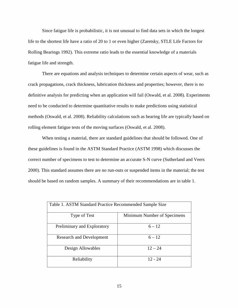
In the area of reliability engineering it is necessary to be confident that a component or system of components will not fail under use for safety and cost reasons. One major mechanism of failure to a mechanical component is fatigue. This is the repetitious motion of loading and unloading of the material, typically below the ultimate tensile strength of the material, which ultimately leads to a catastrophic failure. To ensure this does not happen, engineers design components based on tests to determine the life of these components. These tests are typically conducted on a bench type tester in which a sample it subjected to tension and compression, or supported in a rotational machine in which a load is applied to one end to simulate constant bending. The results from these tests tell how long it is predicted that the part will last. This data however is not always complete. It sometimes happens that not every specimen tested actually makes it to failure; the un-failed specimens are known as suspensions. This can occur for numerous reasons. Methods currently exist for handling suspensions; however these methods require tedious hand calculations and interpolations from multiple graphs which are limited in availability. Presented here are five methods utilizing the Monte Carlo technique in a computer simulation based on Weibull-Johnson confidence numbers that take into account suspensions. This simulation allows for data from an existing experiment to be used as inputs and either validate the findings or bring attention for more testing. The model allows for two different data sets containing suspensions to be analyzed and determine with statistical confidence whether or not there is a difference between the two populations. INDEX WORDS: Fatigue, Monte Carlo, Weibull, confidence number, suspensions
DEVELOPMENT AND VALIDATION OF PROBABILISTIC
FATIGUE MODELS CONTAINING OUT-LIFE SUSPENSIONS
by
NOEL MURRAY
B.S., Georgia Southern University, 2008
A Thesis Submitted to the Graduate Faculty of Georgia Southern University in Partial
“Neglecting suspensions and assuming a complete test of magnitude equal to failure
index amounts to assigning too high a population rank to each failed item. This causes the
Weibull plot to be shifted upward, making the life estimate more conservative than necessary”
33
(Johnson, The Statistical Treatment of Fatigue Experiments 1964). This would lead to over
designing components and again wasting material and money.
Limitations of Johnson’s Method
The use of Johnson’s method for determining the difference of two populations has fallen
out of wide spread use due to the difficulty of his interpolating between his figures and the lost
literature on how he arrived at his method (Vlcek, Hendricks and Zaretsky, Probabilistic
Analysis for Comparing Fatigue Data Based on Johnson-Weibull Parameters 2007).
The problem with Johnson’s method is that he has a limited number of Weibull slopes
and degrees of freedom of which his charts allow for determining confidence numbers. His
methods and equations for coming up with these charts has been lost. His method is not easily
used for many points of data and it can be quite time consuming.
Monte Carlo Methods
The incorporation of Weibull-Johnson Monte Carlo simulations to the statistical analysis
field gave another dimension: another means of calculating and predicting the outcomes of
components. The application of a Monte Carlo simulation to fatigue data to determine statistical
reliability and confidence numbers has been demonstrated in the simulation of fatigue lives of
bearings (Vlcek, Zaretsky and Hendricks, Test Population Selection From Weibull-Based, Monte
Carlo Simulations of Fatigue Life 2008), (Vlcek, Hendricks and Zaretsky, Determination of
Rolling-Element Fatigue Life From Computer Generated Bearing Tests 2003), (McBride 2011).
34
Generic Monte Carlo Simulation
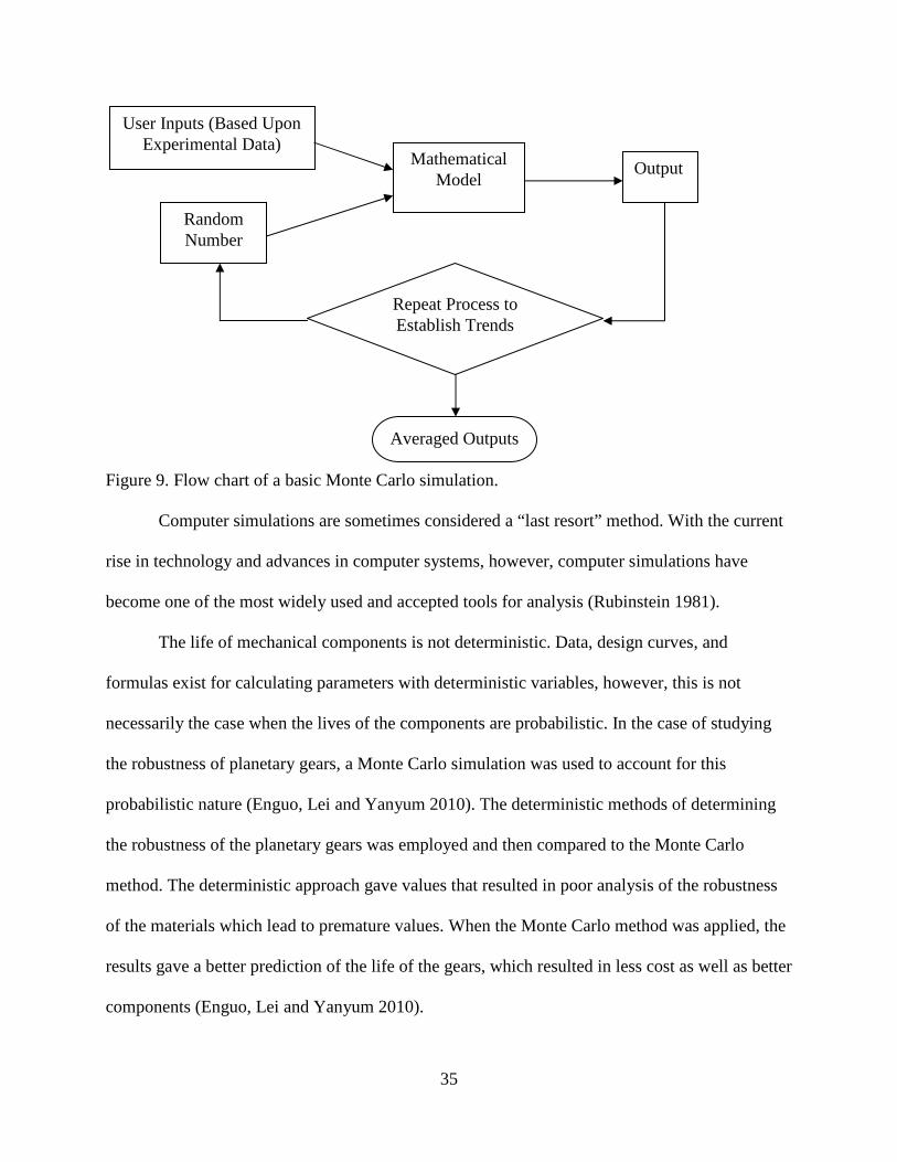
A Monte Carlo simulation is a mathematical process that combines user inputs and
random variable input(s) to a mathematical equation to simulate possible outcomes. This random
process is repeated many times to establish trends, if not absolute magnitude (Rubinstein 1981).
A flowchart showing the basic steps of a Monte Carlo simulation is shown in figure 9.
The term Monte Carlo was first introduced by von Neumann and Ulam during World
War II as a secret code word at Los Alamos. It was in reference to the gambling casinos in
Monte Carlo, Monaco (Rubinstein 1981). According to Haldar (Haldar and Mahadevan 2000),
the Monte Carlo simulation is comprised of six elements: “1) defining the problem in terms of all
the random variables; 2) quantifying the probabilistic characteristics of all the random variables
in terms of their PDFs or PMFs and the corresponding parameters; 3) generating the values of
these random variables; 4) evaluating the problem deterministically for each set of realizations of
all the random variables, that is, numerical experimentation; 5) extracting probabilistic
information from N such realizations; and 6) determining the accuracy and efficiency of the
simulation.”
35
Figure 9. Flow chart of a basic Monte Carlo simulation.
Computer simulations are sometimes considered a “last resort” method. With the current
rise in technology and advances in computer systems, however, computer simulations have
become one of the most widely used and accepted tools for analysis (Rubinstein 1981).
The life of mechanical components is not deterministic. Data, design curves, and
formulas exist for calculating parameters with deterministic variables, however, this is not
necessarily the case when the lives of the components are probabilistic. In the case of studying
the robustness of planetary gears, a Monte Carlo simulation was used to account for this
probabilistic nature (Enguo, Lei and Yanyum 2010). The deterministic methods of determining
the robustness of the planetary gears was employed and then compared to the Monte Carlo
method. The deterministic approach gave values that resulted in poor analysis of the robustness
of the materials which lead to premature values. When the Monte Carlo method was applied, the
results gave a better prediction of the life of the gears, which resulted in less cost as well as better
components (Enguo, Lei and Yanyum 2010).
User Inputs (Based Upon Experimental Data)
Random Number
Mathematical Model
Output
Repeat Process to Establish Trends
Averaged Outputs
36
Monte Carlo Method used for Pattern Recognition
“The design, analysis, and verification and validation of a spacecraft rely heavily on
Monte Carlo simulations” (Restrepo and Hurtado n.d.). Space travel is a very expensive
endeavor and requires many engineering man hours to ensure the safety and reliability of a
spacecraft. With the incredibly high expenses, it is not possible to test every system and
determine all the possible outcomes. Testing, therefore, is limited. Monte Carlo simulations
allow engineers to input different variables and let the program run to generate different random
outcomes (Restrepo and Hurtado n.d.). This simulation, run long enough, could potentially
display most of the possible outcomes of disasters and allow the engineers to design accordingly.
There is, however, one problem with this method that was addressed in (Restrepo and Hurtado
n.d.). With the enormity of possibilities of outcomes it can become very difficult to go through
all the data. Restrepo and Hurtado have developed a plan to attack large amounts of data from a
Monte Carlo simulation using pattern recognition. “Given enough time the Monte Carlo
approach allows analysts to identify most of the individual design variables that influence certain
system failures” (Restrepo and Hurtado n.d.). It typically, however, is not an individual
parameter that causes a failure; it is a series of complex anomalies that lead to system failure
(Restrepo and Hurtado n.d.). It is this series of events that an engineer must try to predict to aid
in the design process of the system. “The goal of a Monte Carlo simulation is to understand all
critical design sensitivities that may prevent the design from meeting requirements” (Restrepo
and Hurtado n.d.).
Monte Carlo simulations can give an extreme amount of data. This leaves the engineer to
sift through great quantities of data. One drawback to this is that the engineer needs some kind of
already known intuition about the system to make judgment calls. Also, it is required to have a
37
sound knowledge in the area of the research. Restrepo and Hurtado (Restrepo and Hurtado n.d.)
have devised a method to escape this problem.
To evaluate the accuracy of more sophisticated statistical techniques, or to verify a new
technique, simulation is routinely used to independently evaluate the underlying probability of
failure (Haldar and Mahadevan 2000). “In the simplest form of the basic simulation, each
random variable in a problem is sampled several times to represent its real distribution according
to its probabilistic characteristics. Using many simulation cycles gives the overall probabilistic
characteristics of the problem, particularly when the number of cycles N tends to infinity. The
simulation technique using a computer is an inexpensive way (compared to laboratory testing) to
study the uncertainty in the problem” (Haldar and Mahadevan 2000). The most commonly used
simulation for this purpose is the Monte Carlo simulation. Engineers have been using this tool
because of its ease of use and its accuracy of results. A strong background in statistics and
probability is not needed to develop a Monte Carlo simulation. These are the reasons why
engineers use Monte Carlo simulations for evaluating the risk and reliability of complicated
systems (Haldar and Mahadevan 2000).
Preventive Maintenance
Preventive maintenance schedules are crucial to ensuring machines and systems operate
properly and that no harm is done. Preventive maintenance can be defined as “a fundamental,
planned maintenance activity designed to improve equipment life and avoid any unplanned
maintenance activity” (Wireman 2008). With the analysis of fatigue data it is possible to
determine these preventive maintenance schedules as well as warranty information.
38
The Space Shuttle is one example of the critical importance to ensure human safety and
machine reliability. The space shuttle was designed to function for 100 flights per shuttle without
maintenance or inspection (Oswald, et al. 2008). One system, in particular, is the body flap
actuators on the space shuttle. There are four actuators on each shuttle (two per wing). After
several flights of the shuttle, the bearings of these actuators were inspected for wear. Due to the
varying degrees of wear, analysis had to be performed to determine proper timing of removal and
replacement of these bearings (Oswald, et al. 2008).
This analysis was performed and the objectives of the research were: “a) experimentally
duplicate the operating conditions of the space shuttle body flat actuator input shaft ball bearings;
b) generate, under these simulated conditions, a statistical data base codifying bearing wear; c)
determine the usable life of the actuator bearings based on a two-parameter Weibull distribution
function for the bearings using strict-series system reliability; and d) compare these results to
field data from the space shuttle fleet (Oswald, et al. 2008).” The statistical methods to analyze
this data was both Weibull (Weibull 1951) and Johnson (Johnson, The Statistical Treatment of
Fatigue Experiments 1964), (Johnson, Theory and Technique of Variation Research 1964).
These methods have been in use by NASA for over 50 years in the area of failure analysis of
bearings and gears in which a large database now exists (Oswald, et al. 2008).
Using the probabilistic method on the actuators, it was predicted that the bearing would
fail after 20 missions. This was in close agreement to the actual failure at 22 missions (Oswald,
et al. 2008). Of 116 missions between 1981 and 2006, it was reported that only one actuator
bearing had to be replaced due to excessive wear (Oswald, et al. 2008).
During the experiment, one of the tests conducted to determine the life of a bearing
included six bearings in which sudden death testing was used that resulted in three of the six
39
bearings failing (Oswald, et al. 2008). The analysis used to incorporate the suspended items was
that of Johnson (Johnson, The Statistical Treatment of Fatigue Experiments 1964).
Along with testing for failure comes the knowledge of how to prevent failure in the first
place. During failure testing, engineers learn methods to prevent failure. Different tolerances and
lubrication methods lead to longer failure lives. The only way to prevent or postpone failure is to
maintain the machine. Proper maintenance schedules need to be written and enforced. Failure
tests, proper lubrication, and maintenance schedules are one way to prevent failure.
Summary
Fatigue has been studied since the mid 1800’s when train axles started breaking
unexpectedly. It turned out that this phenomenon was probabilistic and could not be precisely
predicted. In the 1930’s Weibull developed a method to analyze this probabilistic occurrence.
Although this method has been criticized by mathematicians it has worked for years and
engineers still use it. Leonard Johnson developed a way of ranking two populations of fatigue
data. From his method it is possible to statistically determine whether or not one population is
better than the other.
Recently, with the advent of computers, Monte Carlo simulations have been developed to
analyze fatigue data. A Monte Carlo simulation uses a limited number of predetermined inputs
and random numbers to simulate possible outcomes. This means of comparing fatigue data has
been demonstrated to work.
40
Chapter 3
Method
Introduction
The purpose of this research is to compare fatigue data sets containing out-life
suspensions via a Monte Carlo simulation. Existing methods for handling such suspensions can
be tedious, relying heavily upon graphical interpretation and interpolation of design curves
(Johnson, The Statistical Treatment of Fatigue Experiments 1964). This current project takes
advantage of technological computing power to handle a statistically significant number of
simulations.
A model was developed to simulate experimental fatigue data that contains suspensions.
A Monte Carlo simulation was written in Visual Basic, to interface with Microsoft Excel, to
simulate fatigue lives using a “bin” model developed by Vlcek, Hendricks and Zaretsky (Vlcek,
Hendricks and Zaretsky, Determination of Rolling-Element Fatigue Life From Computer
Generated Bearing Tests 2003). Different suspension models were evaluated. The models
differed in how the failure index (number of failed samples or total number samples tested) was
modeled prior to determining the L10 life for the data set. A relative ranking counting method
similar to that demonstrated by McBride, Vlcek, and Hendricks (McBride 2011) was used to
determine the relative confidence numbers associated with each suspension method. The
simulation was repeated a statistically significant number of times (10,000). For validation of
the model, the simulated confidence numbers were compared to those graphically determined for
two experimental data sets that were available in the literature (Townsend, Zaretsky and
41
Anderson, Comparison of Modified Vasco X-2 with AISI 9310 - Preliminary Report 1977),
(Townsend and Zaretsky, Comparisons of Modified Vasco X-2 and AISI 9310 Gear Steels
1980).
Monte Carlo Simulation - Weibull Equation, Confidence Numbers, and “Bin” Model
The model was generated by combining three statistical methods already in existence.
The first was the use of the Weibull equation (equation 1) to determine a life. Using a random
number generator, a number between 1 and 1000 was generated. This number represented the
order in which the sample failed (this is known as the “bin” model and will be discussed in more
detail in the next section). From this the order number was converted to a rank using equation 3.
This number subtracted from 1 gave the survivability (S) of the sample. Then, using the Weibull
slope and characteristic life as determined from experimental data, a virtual life can be solved for
algebraically.
The second method incorporated into the model was developed by Johnson (Johnson,
The Statistical Treatment of Fatigue Experiments 1964). Johnson developed a way to
statistically predict whether or not one material was better than another. He did this through
confidence numbers. If two materials were analyzed, and a confidence number of 90 or higher
was determined, then it implies that there is a statistical difference between the two materials.
Although his graphical method of calculating confidence numbers was not incorporated into this
model, the idea behind a confidence number was—how many times out of one hundred, one
probabilistic value was greater than another. Johnson also developed a method for incorporating
42
suspensions into the determination of a confidence number, and demonstrated the importance of
taking suspensions into consideration instead of just dismissing them.
The third method incorporated into this model was that of Vlcek et al. (Vlcek, Hendricks
and Zaretsky, Probabilistic Analysis for Comparing Fatigue Data Based on Johnson-Weibull
Parameters 2007), (Vlcek, Hendricks and Zaretsky, Relative Ranking of Fatigue Lives of
Rotating Aluminum Shafts Using L10 Weibull-Johnson Confidence Numbers 2008), (Vlcek,
Hendricks and Zaretsky, Determination of Rolling-Element Fatigue Life From Computer
Generated Bearing Tests 2003), (McBride 2011). Vlcek et al. developed what is referred to as a
virtual bin model. The bin model is a virtual bin of 1000 specimens that are assumed to have
been tested to failure. The lives of these samples are not known at this time, however, the order
in which they failed is known, and each sample has an order number from 1 to 1000 associated
with the order in which it failed. With this order number, it is possible to determine the
survivability of the sample using the median rank equation (equation 3). If the Weibull slope (m)
and characteristic life (Lβ) are known, then the simulated life is the only unknown in the Weibull
equation (equation 1), and can be algebraically solved for.
Another method used that was developed by Vlcek et al. was that of numerically
counting simulated lives to arrive at a confidence number. Since a confidence number is defined
as the number of times out of 100 one material will be better than another, with a Monte Carlo
simulation generating 100 virtual lives it is possible to count how many times the life of one
material is greater than the other.
The last method used by Vlcek et al. in this simulation was the development of curve fit
equations, which were derived from Johnson’s figures, to calculate a confidence number. These
equations were incorporated into the simulations, to use the variables generated, to calculate a
43
confidence number. This added one more dimension for comparison of confidence numbers.
Ultimately three confidence numbers were able to be compared to determine whether or not one
material was better than the other.
Bin Model Monte Carlo Simulation
The objective of the Monte Carlo technique in this application is to acquire virtual lives
from random numbers between 1 and 1000 which represent samples in a bin ordered in which
they failed. These numbers were converted to lives by use of the rank equation (equation 3) and
the Weibull equation (equation 1).
These random numbers represent the order in which the gears would have failed had all
1,000 been tested. For example, if the random number generator used by the simulation
generates the number 784, this would represent the 784th sample to fail in the bin of 1,000. Since
the true life of the 784th sample that failed is not known, it will be sequentially ordered against
the other samples in its bin. Sample 1 will have the shortest life, and sample 1,000 will have the
longest life.
The random number generator itself does not have a method for determining how many
of a certain number it picks. For example, it is possible that the number 256 gets generated twice.
This is not desired because it is not possible to have two samples with the order number 256.
This issue was addressed to ensure unique random numbers. No two samples can have the same
rank. A Visual Basic Module in Excel was written to ensure that all random numbers or parts
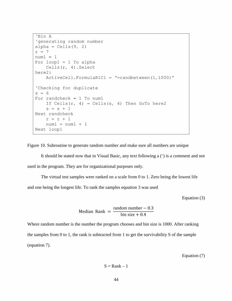
pulled from the bin were unique in a test set. This module can be seen in Figure 10.
44
Figure 10. Subroutine to generate random number and make sure all numbers are unique
It should be stated now that in Visual Basic, any text following a (‘) is a comment and not
used in the program. They are for organizational purposes only.
The virtual test samples were ranked on a scale from 0 to 1. Zero being the lowest life
and one being the longest life. To rank the samples equation 3 was used
Equation (3)
MedianRank = random number− 0.3
bin size+ 0.4
Where random number is the number the program chooses and bin size is 1000. After ranking
the samples from 0 to 1, the rank is subtracted from 1 to get the survivability S of the sample
(equation 7).
Equation (7)
S = Rank – 1
‘Bin A ‘generating random number alpha = Cells(9, 2) r = 7 num1 = 1 For loop1 = 1 To alpha Cells(r, 4).Select here2: ActiveCell.FormulaR1C1 = “=randbetween(1,1000)” ‘Checking for duplicate s = 6 For randcheck = 1 To num1 If Cells(r, 4) = Cells(s, 4) Then GoTo here2 s = s + 1 Next randcheck r = r + 1 num1 = num1 + 1 Next loop1
45
Lives are assigned to the virtual samples based on the experimental data using the Weibull
equation.
Equation (1)
ln ln1
� = � ln����
The rank from the simulation results in survivability S. The Weibull slope m and characteristic
life Lβ come from previously available experimental data. The virtual life at a survivability
probability S can be calculated after plugging these three variables into equation 1. The lives,
still in order from shortest lived to longest lived, were then ranked again. This time they were
ranked according to the test population size. If 20 samples were used in the experiment, then in
the ranking equation, 20 was used for the population size n, and instead of a random number, 1
to the sample size was used; in this case, from 1 to 20 (equation 8).
Equation (8)
Rank = number− 0.3
20+ 0.4
The survivability S, or percent of samples that survived, is again solved for by using equation 7.
The lnln (1/S) is plotted as a function of the ln (L). lnln (1/S) is plotted on the ordinate and ln (L)
is plotted on the abscissa. As a result, fatigue data plots as a relatively straight line on Weibull
paper, and a fitted curve is determined using a least squares fit. The Weibull slope, characteristic
life, L10 life, L50 life, and mean life are results of this plot. Figure 11 is a flowchart of the
simulation based on a bin model.
46
Figure 11. Flowchart of Monte Carlo simulation based on bin model
Numerically Counting Confidence Numbers
A confidence number determined by the simulation (numerical counting method) was
accomplished by generating 100 L10 lives for two different simulated materials and counting the
number of times the L10 life associated with one population was greater than the other out of 100
comparisons. Since the program generates virtual L10 lives these lives were counted to see how
many times population A has a longer life than population B. The number of times out of 100
that A is better than B and the number of times out of 100 that B is better than A was outputted
User input: Weibull slope,
characteristic life, number of samples
Convert random ranks to fatigue life with Weibull equation
Plot fatigue lives on a Weibull plot to
determine L10 and slope Pull number of samples randomly from bin.
Generate random number between 1-1000 equal to
number of samples Repeat 100 times for each population to determine
confidence number
Repeat process 10,000 times to establish trends
Averaged outputs
47
to the summary table. The greater of the two numbers is the confidence number. If this number is
greater than 90 then it states that there is a significant difference between the two populations. A
flowchart of the simulation determining a confidence number by the numerical counting method
is shown in figure 12.
48
Figure 12. Flowchart of Monte Carlo simulation counting method.
Input known variables for bin A and bin B
Generate random numbers from 1 to 1000
Rank random numbers from 0 to 1
Survivability = 1 - rank
Solve Weibull equation for L
Plot ln(L) vs. lnln(1/S) to solve for Weibull slope and L10
Output Weibull slope and L10 for both bins
Count how many times L10
of A is bigger than L10 of B
Repeat 100 times
Repeat 10,000 times
Average outputs
It was determined which
bin B and then counting the number of times the result
result is greater than one then L10
shown in figure 13.
Figure 13. Subroutine for numerically counting a confidence number
A screen shot of the output of the numerical counting method is shown in figure
Figure 14. Screen shot of output of counting confidence numbers
This confidence number mo
specimens in the original experiment failed. However for the purpo
'L10A / L10B
Cells(60, Column) = Cells(6, Column) / Cells(14, Co lumn) 'Counting which is bigger, L10A or L10B If Cells(60, Column) > 1 Then countL10 = countL10 + 1 Else countL10B = countL10 End If Cells(68, 2) = countL10Cells(69, 2) = countL10B
49
which was greater by dividing the L10 life of bin A by the L
bin B and then counting the number of times the result was greater than or less than one. If the
10 of A was greater, and vice versa for B. This counting method is
Subroutine for numerically counting a confidence number
A screen shot of the output of the numerical counting method is shown in figure
Screen shot of output of counting confidence numbers
This confidence number model works well for experimental data in which all fatigue
specimens in the original experiment failed. However for the purpose of this research a new
Cells(60, Column) = Cells(6, Column) / Cells(14, Co lumn)
'Counting which is bigger, L10A or L10B If Cells(60, Column) > 1 Then
countL10 = countL10 + 1
countL10B = countL10 B + 1
Cells(68, 2) = countL10 Cells(69, 2) = countL10B
life of bin A by the L10 life of
s greater than or less than one. If the
This counting method is
A screen shot of the output of the numerical counting method is shown in figure 14.
del works well for experimental data in which all fatigue
se of this research a new
Cells(60, Column) = Cells(6, Column) / Cells(14, Co lumn)
50
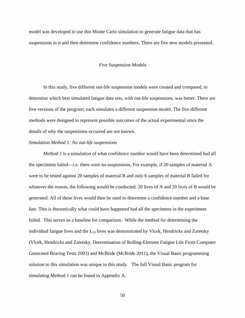
model was developed to use this Monte Carlo simulation to generate fatigue data that has
suspensions in it and then determine confidence numbers. There are five new models presented.
Five Suspension Models
In this study, five different out-life suspension models were created and compared, to
determine which best simulated fatigue data sets, with out-life suspensions, was better. There are
five versions of the program; each simulates a different suspension model. The five different
methods were designed to represent possible outcomes of the actual experimental since the
details of why the suspensions occurred are not known.
Simulation Method 1: No out-life suspensions
Method 1 is a simulation of what confidence number would have been determined had all
the specimens failed—i.e. there were no suspensions. For example, if 20 samples of material A
were to be tested against 20 samples of material B and only 6 samples of material B failed for
whatever the reason, the following would be conducted. 20 lives of A and 20 lives of B would be
generated. All of these lives would then be used to determine a confidence number and a base
line. This is theoretically what could have happened had all the specimens in the experiment
failed. This serves as a baseline for comparison. While the method for determining the
individual fatigue lives and the L10 lives was demonstrated by Vlcek, Hendricks and Zaretsky
(Vlcek, Hendricks and Zaretsky, Determination of Rolling-Element Fatigue Life From Computer
Generated Bearing Tests 2003) and McBride (McBride 2011), the Visual Basic programming
solution to this simulation was unique to this study. The full Visual Basic program for
simulating Method 1 can be found in Appendix A.
A screen shot of the inputs for method one can be seen in figure
Figure 15. Sample of the inputs fo
In this figure, A mA is the slope of the experimental
of the experimental data set for material B. L
for material A and LB,B is the characteris
and size B are the sizes of the populations for materials A and B. Trials is the number of times to
run the loop to calculate a confidence number. Remember the simulation runs 100 times to count
how many times (out of 100) one material is better than the other. Trials* is the number of times
to run the entire program to establish trends. All five methods were run a total of 10,000 times.
51
A screen shot of the inputs for method one can be seen in figure 15.
. Sample of the inputs for method 1
is the slope of the experimental data set for material A and B m
of the experimental data set for material B. LB,A is the characteristic life for the experimental data
is the characteristic life for the experimental data for material B. Size A
and size B are the sizes of the populations for materials A and B. Trials is the number of times to
run the loop to calculate a confidence number. Remember the simulation runs 100 times to count
many times (out of 100) one material is better than the other. Trials* is the number of times
to run the entire program to establish trends. All five methods were run a total of 10,000 times.
data set for material A and B mB is the slope
is the characteristic life for the experimental data
tic life for the experimental data for material B. Size A
and size B are the sizes of the populations for materials A and B. Trials is the number of times to
run the loop to calculate a confidence number. Remember the simulation runs 100 times to count
many times (out of 100) one material is better than the other. Trials* is the number of times
to run the entire program to establish trends. All five methods were run a total of 10,000 times.
52
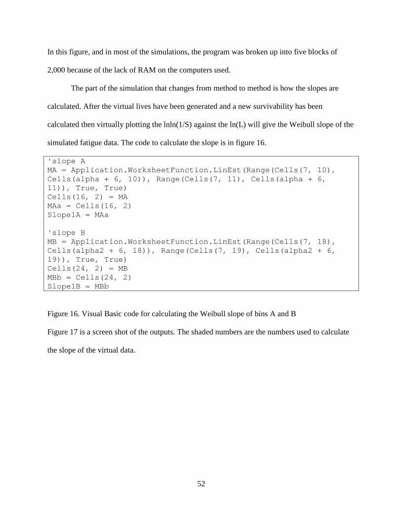
In this figure, and in most of the simulations, the program was broken up into five blocks of
2,000 because of the lack of RAM on the computers used.
The part of the simulation that changes from method to method is how the slopes are
calculated. After the virtual lives have been generated and a new survivability has been
calculated then virtually plotting the lnln(1/S) against the ln(L) will give the Weibull slope of the
simulated fatigue data. The code to calculate the slope is in figure 16.
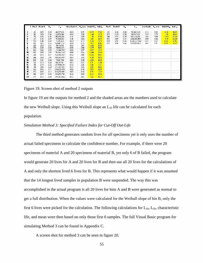
In addition to holding all the values from the calculations, the summary page is where the
numerical counting takes place for the Monte Carlo method of determining a confidence number.
All the L10 lives are counted and determined how many of bin A were greater than bin B.
The Visual Basic Macro of the Simulation before Suspensions Incorporated
The model was developed using Visual Basic for Applications in Microsoft Excel. Excel
was the program of choice because of its ability to handle and organize large amounts of data. It
was also possible to interface with the Visual Basic code through the spreadsheet.
Visual Basic in Excel was developed to make handling small tasks easier. One method of
doing this is by using a macro in Excel. A macro was constructed, for simplicity, by clicking the
“Record Macro” button and following a sequence of steps for whatever task needs to be
completed. The macro is assigned a shortcut key, ctrl+(a letter). For example, if “Record Macro”
was pressed, then the user clicked on an empty cell, and entered the command to take the
average of a series of numbers, and then highlight a series of numbers and pressed enter, then
clicked stop recording, the user would be able to repeat this process by simply hitting the macro
short key.
Once a quick “record” macro has been constructed it is then possible to access the macro
and edit it using Visual Basic code. This is how this model was constructed.
The program was constructed over a number of weeks in small modules. Each module
would be run, and then compared to hand calculations to be sure the code was correct and then
the next module would be added on until the entire program ran as one unit. The initial set up
was on the first page of the spread sheet as shown in figure 29.
Figure 29. Screen shot of simulation inputs
There were cells assigned to values that would be inputted by the user. These inputs
included the Weibull slope for eac
and the number of trials to be run.
First the set of random numbers that represented the number in which the
was generated. The number generator in Visual Basic generated a
1000. To ensure that no two same random numbers appeared in either of the sets generated, a
sub-routine was written that compared each randomly pulled number to those already selected
for the data set (figure 10). If found to
in question was discarded, another pulled, and uniqueness again established.
70
shot of simulation inputs.
There were cells assigned to values that would be inputted by the user. These inputs
included the Weibull slope for each bin, the characteristic life for each bin, the size of each bin,
and the number of trials to be run.
First the set of random numbers that represented the number in which the
was generated. The number generator in Visual Basic generated a random number between 1 and
1000. To ensure that no two same random numbers appeared in either of the sets generated, a
routine was written that compared each randomly pulled number to those already selected
. If found to equal one of the previously pulled numbers, the number
in question was discarded, another pulled, and uniqueness again established.
There were cells assigned to values that would be inputted by the user. These inputs
h bin, the characteristic life for each bin, the size of each bin,
First the set of random numbers that represented the number in which the sample failed
random number between 1 and
1000. To ensure that no two same random numbers appeared in either of the sets generated, a
routine was written that compared each randomly pulled number to those already selected
equal one of the previously pulled numbers, the number
71
The random numbers were then ordered from smallest to largest to be ranked. To rank
them equation 3 was used. This rank was then turned in to a survivability value by subtracting it
from 1. This survivability was then incorporated into the Weibull equation (equation 1), along
with the Weibull slope and characteristic life as reported in the literature to determine a life. The
code for determining a rank, then survivability, then a life is shown in figure 30.
\
Figure 30. Subroutine for determining a life from random number.
Once the lives were established, a new rank was calculated based upon the size of the
pulled population rather than 1000, this time from 1 to population size. Once the rank was
established again, the survivability associated with each life was calculated. The lnln(1/S) and
the ln(L) were calculated to determine a Weibull slope for the generated data. The code for
determining the new rank, new survivability, lnln(1/S), and ln(L) is shown in figure 31.
For loop5 = 1 To alpha 'Rank A Cells(r1, c1) = (Cells(r1, c2) - 0.3) / (1000 + 0.4) 'S of A Cells(r1, c4) = 1 - Cells(r1, c1) SA = Cells(r1, c4) 'Life of A A1 = Application.WorksheetFunction.Ln(1 / S A) B1 = Application.WorksheetFunction.Ln(A1) CA = Exp(B1 / Cells(3, 2)) * Cells(6, 2) Cells(r1, c6) = CA r1 = r1 + 1 Next loop5
72
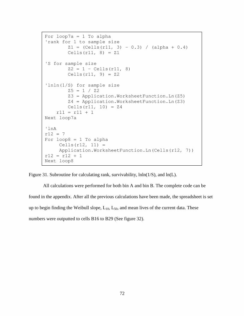
Figure 31. Subroutine for calculating rank, survivability, lnln(1/S), and ln(L).
All calculations were performed for both bin A and bin B. The complete code can be
found in the appendix. After all the previous calculations have been made, the spreadsheet is set
up to begin finding the Weibull slope, L10, L50, and mean lives of the current data. These
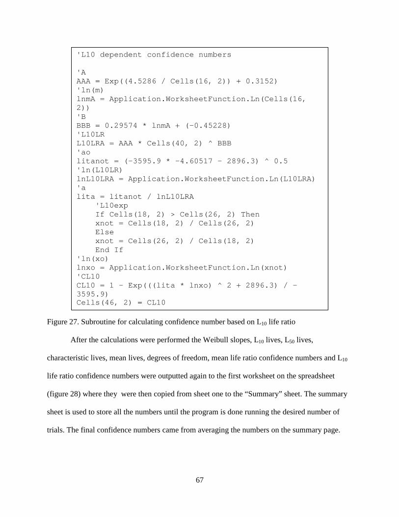
numbers were outputted to cells B16 to B29 (See figure 32).
For loop7a = 1 To alpha 'rank for 1 to sample size Z1 = (Cells(r11, 3) - 0.3) / (alpha + 0.4) Cells(r11, 8) = Z1 'S for sample size Z2 = 1 - Cells(r11, 8) Cells(r11, 9) = Z2 'lnln(1/S) for sample size Z5 = 1 / Z2 Z3 = Application.WorksheetFunction.Ln(Z5) Z4 = Application.WorksheetFunction.Ln(Z3) Cells(r11, 10) = Z4 r11 = r11 + 1 Next loop7a 'lnA r12 = 7 For loop8 = 1 To alpha
order to make the Vasco X-2 suitable for helicopter transmission gears, the carbon content was
lowered and then the material was case hardened leaving a softer core. The objectives of their
research were to a) determine the performance of spur gears made from the new material
modified Vasco X-2, b) compare the fatigue lives of the old material AISI 9310 against the new
material modified Vasco X-2, and c) to compare the hot hardness retention of the two materials.
This was going to be accomplished by testing the spur gears with different heat treatments,
rolling contact fatigue tests, and hardness tests.
The specific test this current research was concerned with was the rolling element test. In
this test a 3 inch long rod with 0.375 inch diameter was inserted into the rolling contact test
apparatus (figure 38). This tester consisted of two rolling discs of 7.5 inch diameter made of
AISI M-50 steel which were heat treated to the same hardness as the samples. The samples were
placed in between the two discs and a load was applied until the sample was able to turn both
discs. Once the discs and sample were in thermal equilibrium the maximum load (700,000 psi)
was applied. The specimen would be rotated at 12,500 rpm until failure occurs. The tester would
shut down automatically by means of a vibration detector. The lives of the specimens, denoted
by number of rotations until failure, were used to calculate a confidence number to determine
which material was more suitable for the application. In the experiment 20 samples of Modified
Vasco X-2 were tested and all 20 of them failed. AISI 9310 also had 20 samples reported as
tested, but only 6 reached failure.
Figure 38. Rotational fatigue tester
Vasco X-2 with AISI 9310 - Preliminary Report
The experiment determined that there was an 84% confidence between the two materials.
This says that 84 times out of 100 AISI 9310 will last longer than Modified Vasco X
According to Johnson (Johnson, The Statistical
number states that there is no statistical difference between the two materials. There must be a
confidence of 90 or greater to be determined statistically different. A summary of these results is
in table 21.
97
. Rotational fatigue tester (Townsend, Zaretsky and Anderson, Comparison of Modified
Preliminary Report 1977)
The experiment determined that there was an 84% confidence between the two materials.
This says that 84 times out of 100 AISI 9310 will last longer than Modified Vasco X
(Johnson, The Statistical Treatment of Fatigue Experiments 1964)
number states that there is no statistical difference between the two materials. There must be a
confidence of 90 or greater to be determined statistically different. A summary of these results is
(Townsend, Zaretsky and Anderson, Comparison of Modified
The experiment determined that there was an 84% confidence between the two materials.
This says that 84 times out of 100 AISI 9310 will last longer than Modified Vasco X-2.
Treatment of Fatigue Experiments 1964) this
number states that there is no statistical difference between the two materials. There must be a
confidence of 90 or greater to be determined statistically different. A summary of these results is
98
Table 21. Fatigue life results from Comparison of Modified Vasco X-2 with AISI 9310
The results of the gear tests of Townsend and Zaretsky (Townsend, Zaretsky and
Anderson, Comparison of Modified Vasco X-2 with AISI 9310 - Preliminary Report 1977) were
that the gears made from AISI 9310 survived on the magnitude of hours with millions of cycles.
Failure occurred due to surface pitting or spalling. The modified Vasco X-2 gears, however, only
survived in the 600,000 range for less than an hour and failure was due to tooth fracture.
A summary of the results is as follows:
1) Crack formation at the tips of the gear teeth during carburizing process of the modified
Vasco X-2 resulted in fracture of the gear teeth after a period of less than one hour
(600,000 revolutions) of operations under test conditions.
2) The lives of the AISI 9310 gears at a 90% probability of survival were 39.3, 19, and 7.1
hours at 222,000 psi, 248,000 psi, and 272,000 psi respectively.
3) Failure of the AISI 9310 gears was by surface pitting with no tooth fracture occurring.
99
4) The rolling element fatigue life of the AISI 9310 was approximately twice that of the
modified Vasco X-2.
5) At temperatures of approximately 300 F there was no significant difference in hot
hardness between the modified Vasco X-2 and AISI 9310 materials.
Summary of Comparisons of Modified Vasco X-2 and AISI 9310 Gear Steels
The second paper used for comparison was Comparisons of Modified Vasco X-2 and
AISI 9310 Gear Steels by Dennis P. Townsend and Erwin V. Zaretsky, 1980 (Townsend and
Zaretsky, Comparisons of Modified Vasco X-2 and AISI 9310 Gear Steels 1980). In this
experiment, again, two different gear materials were tested to see which was superior. The AISI
9310 was compared to three different heat treatments of Modified Vasco X-2. The three different
heat treatments came from three different vendors, Boeing Vertol, NASA, and Curtis-Wright. In
this experiment, gears were tested as opposed to material rods as in the first experiment. The
apparatus used is shown in figure 39. The results of the experiment are shown in table 22.
Figure 39. Gear tester used in original experiment
Modified Vasco X-2 and AISI 9310 Gear Steels 1980)
100
. Gear tester used in original experiment (Townsend and Zaretsky, Comparisons of
and AISI 9310 Gear Steels 1980)
(Townsend and Zaretsky, Comparisons of
101
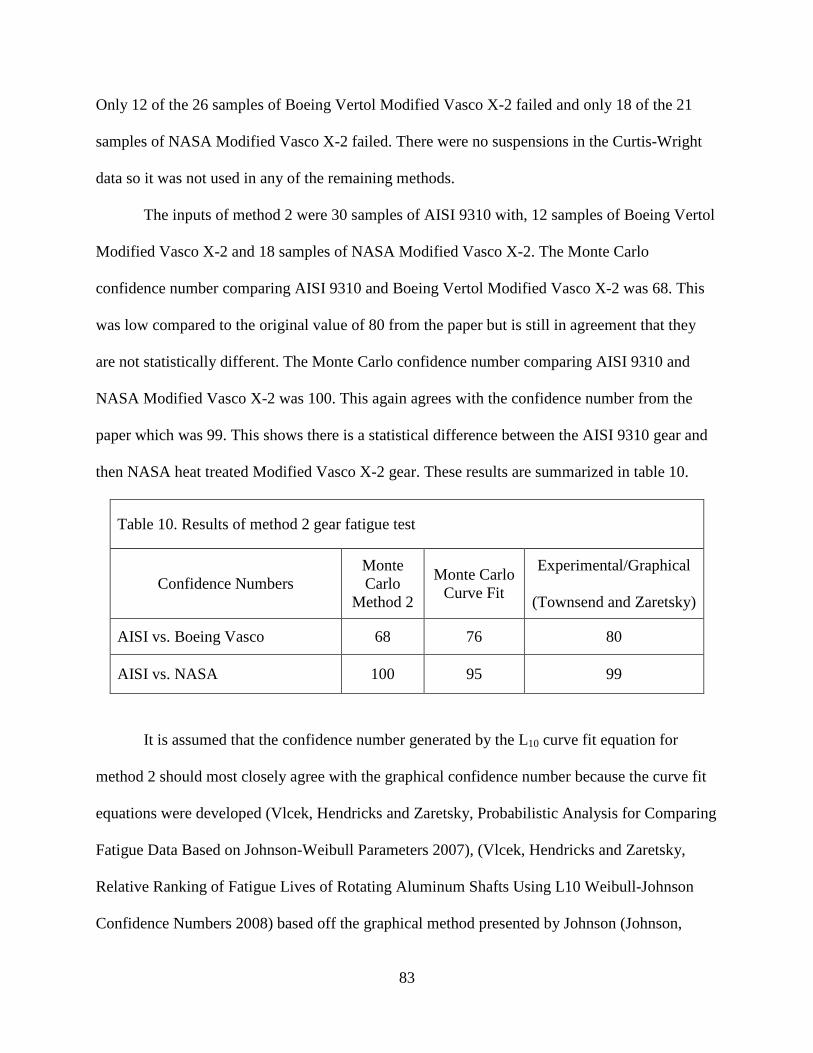
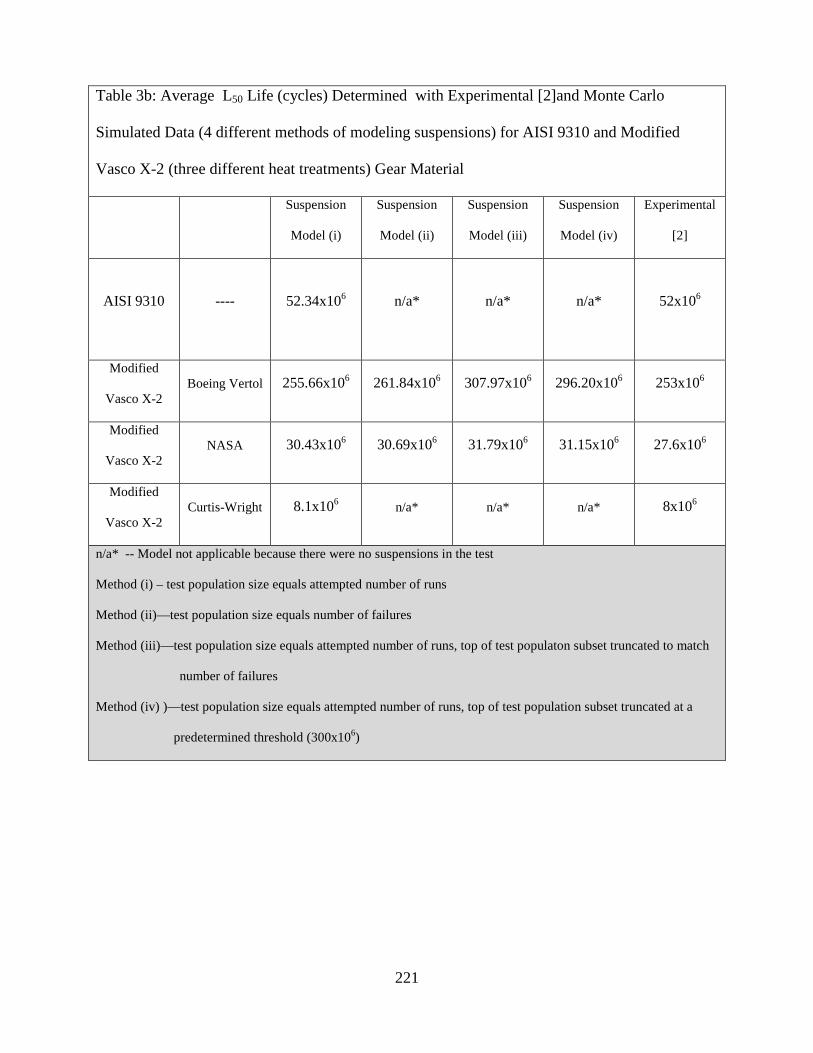
Table 22. Summary of gear fatigue life results from Comparison of Modified Vasco X-2 and AISI 9310 Gear Steels (Townsend and Zaretsky, Comparisons of Modified Vasco X-2 and AISI 9310 Gear Steels 1980)
Material Heat treat
procedure Gear system life, Revolutions Weibull Slope Failure Indexa Confidence
Vasco X-2 Boeing Vertol 38.4x10⁶ 253 x106 1.0 12 of 26 80
NASA 0.8 x10⁶ 27.6 x10⁶ 0.53 18 of 21 99 Curtis-Wright 3.3 x10⁶ 8 x10⁶ 2.1 19 of 19 99
aNumber of fatigue failures out of number of gears tested bPercentage of time that 10-percent life obtained with AISI 9310 gears will have the same relations to the 10-percent life obtained with modified Vasco X-2 gears.
There was no statistical difference between AISI 9310 and the Boeing Vertol heat
treatment of Modified Vasco X-2 with a confidence number of 80, however there was a
statistical difference between AISI 9310 and the NASA and Curtis-Wright heat treated Modified
Vasco X-2, both with confidence numbers of 99. It was reported that all 30 of the AISI 9310
gears failed, and all 19 of the Curtis-Wright gears failed, however, only 12 of the 26 of the
Boeing Vertol gears failed, and only 18 of the 21 of the NASA gears failed. Graphs of the results
are shown in figure 36.
Summary of Original Experimental Results
In the comparison of Modified Vasco X-2 with AISI 9310 rolling contact fatigue test the
original experiment stated that the fatigue life of AISI 9310 was approximately twice that of
Modified Vasco X-2, however, the two materials were not statistically different due to a
confidence number of 84.
This was in agreement with the numbers calculated by methods 1-5. Seven of the ten
confidence numbers were on the correct side of 90 to show no statistical difference, while the
102
other three were 92, which is very close to the cutoff of 90. This leads to a conclusion by the
methods presented that there is no statistical difference between the fatigue lives of AISI 9310
and Modified Vasco X-2.
In comparing AISI 9310 gears to the three different heat treatments of Modified Vasco
X-2 gears, it was shown in the original experiment that Modified Vasco X-2 gears can be
reasonably reliable if extreme quality control in the heat treating process is observed. The results
did show that there was no statistical difference between the AISI 9310 gears and the Modified
Vasco X-2 gears subjected to the heat treatment by Boeing Vertol with a confidence number of
80. The results generated by the Monte Carlo method and the L10 curve fit equations were in
agreement with this number for all five methods. Also the original results showed there was a
statistical difference between the AISI 9310 gears and the Modified Vasco X-2 gears subjected
to the heat treatments by NASA, and Curtis-Wright, both with a confidence number of 99. This
was also in agreement with the results generated by the Monte Carlo and L10 curve fit equations
methods. All five methods gave a confidence number of 100.
Preventive Maintenance
Another reason for the need of fatigue studies is for warranty or preventive maintenance
information. If a company studies the fatigue of one of their components, they will know how
long to warranty that component. A company can determine a warranty based on the failure
analysis of their part, this means that on average their part fails within that frame time. If
someone happens to buy a part that falls below the mean, then they are covered and can get a
103
new part. Likewise, if their part outlasts the warranty then they know they got their money’s
worth because the part is above average and may continue to work for a long time.
Similar to determining warranties, fatigue testing is used to determine preventive
maintenance schedules. If you do not know how long a component lasts, then how do you know
when to change it out? Fatigue testing allows for determining theses schedules with very good
accuracy, depending on the application and what percentage of failure is allowed.
When fatigue tests are performed, typically only between ten and twenty samples are
tested due to high cost and testing time. It was demonstrated in (Vlcek, Zaretsky and Hendricks,
Test Population Selection From Weibull-Based, Monte Carlo Simulations of Fatigue Life 2008)
that for a 30 percent variability in fatigue life data at least 30 to 35 samples must be tested. Any
more samples will give better results, however, even with 200 samples, there is still a 15 percent
variation from maximum life to minimum life (Vlcek, Zaretsky and Hendricks, Test Population
Selection From Weibull-Based, Monte Carlo Simulations of Fatigue Life 2008). People have
fallen victim to simple sample tests to predict what a population will do. It has been standard
practice to perform these tests and acquire the data and then simply take an average of the data
and then that will be the resultant number. This method of testing has been proven to not be
sufficient. When only the average of a sample is taken in to account, certain aspects of the data
are missed. Another misconception in reading data is to graph it and make assumptions visually.
Graphs are made to be read and to put data into visual perspective. It is very easy to over look
the fact that if you were to enlarge the graph, the data points may be lying directly on top of each
other, which would indicate no statistical difference. These aspects of data collection are taken
into account with Johnson’s methodology. A test of ten bearings in a bin of 1,000 could
potentially give unsatisfactory data. The strongest ten in a box could be picked and then it could
104
be assumed that the rest are just as strong, when in reality, if they are put into production
components, they could have disastrous effects.
Summary of Results
There were five models developed to analyze out-life suspensions in fatigue data. It was
shown that methods 1 through 4 were in relatively close agreement with the experimental results
from the literature that were determined graphically. Method 5 was not in agreement. This is
believed to be because the number of samples used in the calculations was very small compared
to the range of lives given, and there was too much variability in the randomness to notice any
trends.
105
Chapter 5
Conclusion
Fatigue
The goal of a mechanical engineer is to design components that last and are safe to use.
To determine whether or not a specific component or material will last, it must be tested. One
such test is a fatigue test. This will give the engineer an idea of how long a component will last
under certain circumstances. The problem with fatigue data is that it is probabilistic and not
deterministic. There is no way to determine exactly when something will fail, however, there
exist methods for predicting when a component will fail.
The first was developed by Waloddi Weibull in the 1950’s. He developed a method for
statistically predicting failure. Following Weibull’s method, Leonard Johnson in the 1960’s
developed a method to determine whether or not one material was statistically different from
another. This method was widely used by engineers; however, it was difficult to calculate due to
the limited graphs he published. This method was taken a step further by Zaretsky, Hendricks,
and Vlcek. They took Johnsons charts and graphs and developed equations to fit them. This
allowed for ease of use to calculate a confidence number. From there, a Monte Carlo simulation
was written using the equations to expand on the experimental data.
Vlcek, Zaretsky, and Hendricks demonstrated the concept of a “bin” model which was
the basis of the Monte Carlo simulations. In this “bin” model it is assumed that there is a
population of failed samples, the exact lives of these samples is not known, however, it is known
106
in what order they failed. This order can be ranked from 0 to 1 and, using the parameters of the
Weibull equation, it is possible to calculate a life for each sample.
The experimental data (Weibull slope, and characteristic life) would be used as inputs
into the program and the program would run thousands of simulations of the original experiment.
This data would then either agree or disagree with the original experiment. This allows engineers
to have valuable data yet not spend a lot of money and time on experimental testing.
These simulations, however, were limited. Not all fatigue tests are run to failure. Some
tests get stopped for numerous reasons. They may get stopped because the engineer has a
specific cut off point that the specimen does not need to exceed, or the power in the building
could go out. Regardless of the reason for the test to stop, it is still valuable data.
This new simulation takes these suspensions into account and gives a statistically
determined confidence number.
Method
The purpose of this research was to develop a model that would allow the statistical
validation of a confidence number for fatigue tests comparing two materials in which out-life
suspensions are present. The method used was a Monte Carlo simulation in which random
numbers are generated, ranked, and then converted to lives using the Weibull equation
(equation 1). This method of analyzing fatigue results has been used in the past, but not to
incorporate suspensions. The goal of the simulations is to cut down on cost and time of fatigue
tests while still having statistically accurate data.
107
Five methods were developed and then compared to known data sets for validation. The
first method was designed to treat the data as if the failure index was that all samples of both
populations failed. This did not directly take into account suspensions but was used for
comparison purposes. This provided some insight into what possibly could have happened had
all samples failed.
The second method was designed to incorporate only failed samples in the calculations.
The failure index of method two was the same as the failure index in the original experiment.
This again did not directly take suspensions into account in the simulation, but did represent
what should be calculated as if done graphically. When calculating a confidence number
graphically, all that is available is the failed samples, and this is what method 2 represented.
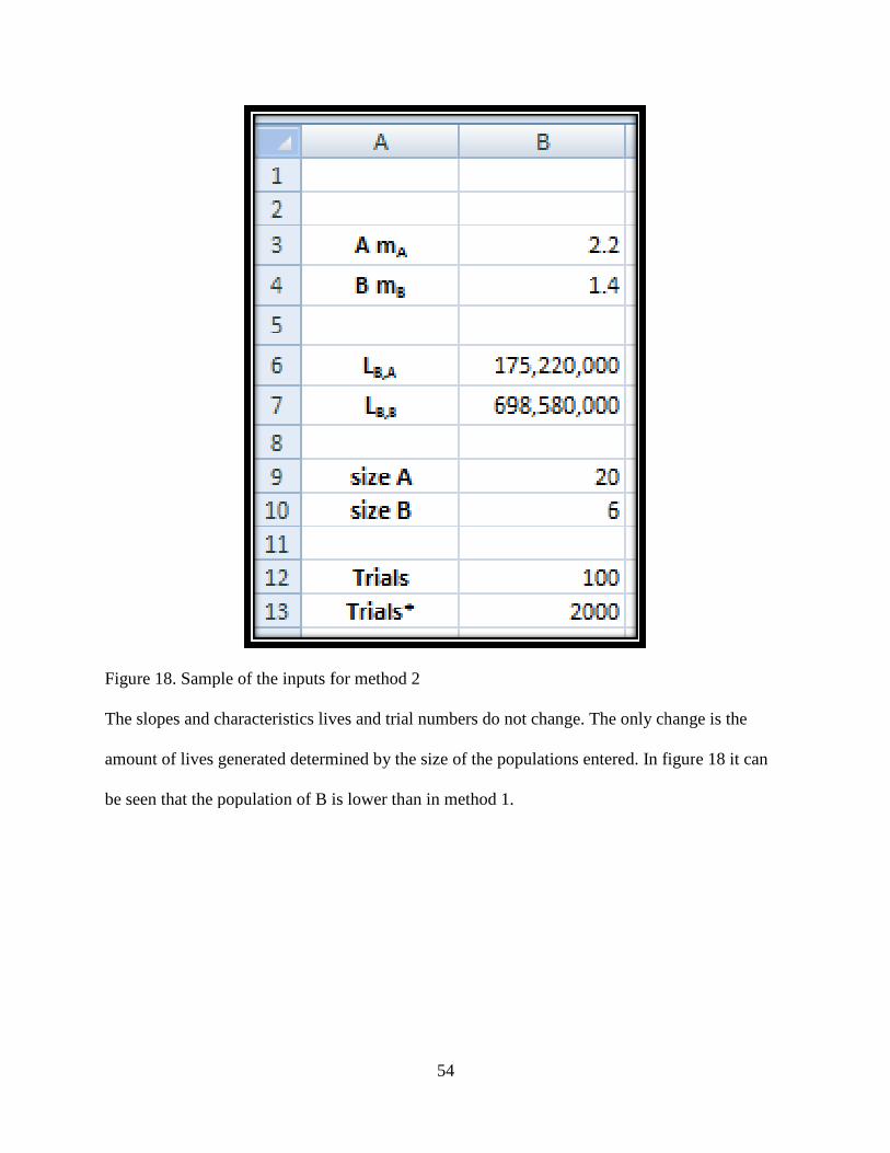
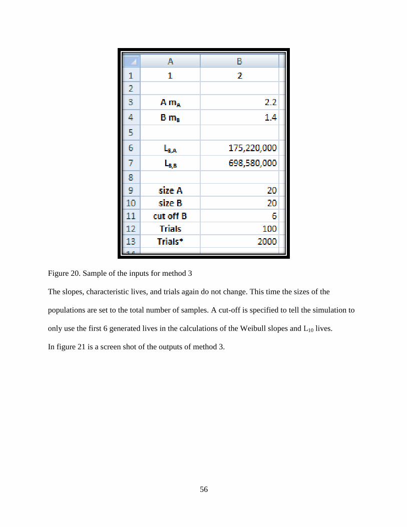
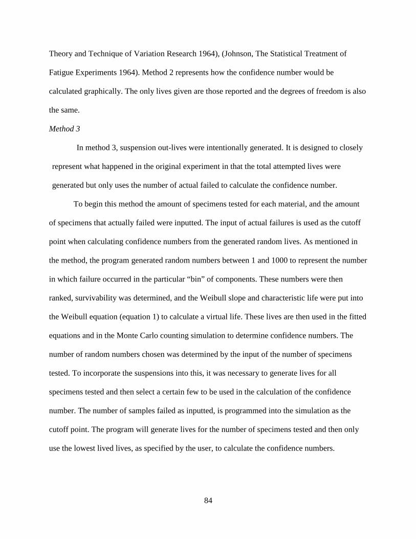
In method 3, suspensions were actually generated. The number of attempted samples was
the number of generated lives; however, the number of samples failed was the number of
generated lives used in the calculations. There was a cutoff sample size incorporated into the
simulation. In generating all the lives it was assumed that there were out-lives not being used in
the calculations. According to the graphs of the original data, it appeared that none of the
samples passed a certain life and this lead to the assumption of out-lives.
Method 4 also made use of generating suspended lives and then used a cutoff to calculate
confidence numbers. This time, however, instead of sample size being the cutoff, a particular life
was the cutoff. Again, the number of lives generated was equal to the number of samples
attempted, yet this time the number of samples used in calculating confidence numbers varied
because the number of samples was determined by how many fell within the range of the cutoff
life.
108
Method 5 was designed to be a hybrid of both methods 3 and 4. The samples generated to
be used in the calculations were forced to a certain number of samples as well as fall within a
certain range of lives.
Results
The results of this model of comparing two fatigue data sets containing suspensions are
repeated in tables 23 and 24.
Table 23. Results of comparing Modified Vasco X-2 and AISI 9310 rolling contact fatigue data
Curve fit confidence numbers vs. Monte Carlo counted confidence numbers based on L10 lives
Material
Method Experimental
1 2 3 4 5
Modified Vasco X-2 vs. AISI 9310
Curve fit 83 79 79 79 74 84
MC 92 78 92 92 52
Table 24. Results of comparing Modified Vasco X-2 and AISI 9310 gear fatigue data
Monte Carlo Counted Confidence Numbers
Material Heat Treatment Method
Experimental 1 2 3 4 5
AISI 9310 ---- ---- ---- ---- ---- ---- ----
Modified Vasco X-2
Boeing Vertol 77 68 77 76 52 80
NASA 100 100 100 100 100 99
Curtis-Wright 100 ---- ---- ---- ---- 99
109
The confidence numbers generated by the simulation, both the Monte Carlo numbers and
the curve fit numbers were in agreement with the original graphical confidence numbers showing
whether two materials were statistically different or not.
Recommendations for Further Study
The next step for incorporating suspensions into a Monte Carlo simulation would be to
reproduce suspensions that are contained within the data. That is suspensions that are not out-
lives. A simulation could be written to use the same bin model and counting method to determine
a confidence number. The user could input how many suspensions there are and then let the
program randomly pick which samples to suspend. This could be repeated to show trends.
This current model could also be adjusted to count the L50 and mean lives. The standard
is to use the L10 life but this could still show trends. If a populations L50 or mean life is
significantly greater this could lead to a conclusion to repeat the experiment if possible to see if
trends repeat.
Another possible future study would be to perform an experiment with fatigue samples
and specify the life at which to use as a cut-off out-life. This way it would be known exactly why
the suspensions occurred and it would be a more accurate way of validating the simulation.
110
References
Askeland, Donald R., and Pradeep P. Phule. The Science and Engineering of Materials. Toronto: Thomson, 2006. ASTM. "Standard Practive for Statistical Analysis of Linear or Linearized Stress-Life (S-N) and Strain-Life (ɛ-N) fatigue Data." ASTM E739-91, 1998. Enguo, Dong, Zhang Lei, and Xing Yanyum. "Robustness analysis for planetary gear based on Monte Carlo method." 2010 WASE International Conference on Information Engineering. IEEE, 2010. 212-215. Haldar, Achintya, and Sankaran Mahadevan. Probability, Reliability, and Statistical Methods in Engineering Design. New York: John Wiley & Sons, 2000. Holland, Frederic A., and Erwin V. Zaretsky. Investigation of Weibull Statistics in Fracture Analysis of Cast Aluminum. Technical Memorandum, Cleveland: NASA, 1989. Johnson, Leonard G. The Statistical Treatment of Fatigue Experiments. New York: Elsevier Publishing Company, 1964. —. Theory and Technique of Variation Research. New York: Elsevier Publishing Company, 1964. Kalpakjian, Serope, and Steven R. Schmid. Manufacturing Engineering and Technology. Upper Saddle River: Pearson Prentice Hall, 2006. McBride, Jacob. Ranking of Fatigue Data Based Upon Monte Carlo Simulated Confidence Number Figures. Thesis, Statesboro: Georgia Southern University, 2011. Naylor, T. J. Computer Simulation Techniques. New York: Wiley, 1966. Norton, Robert L. Machine Design An Integrated Approach. Upper Saddle River: Pearson Prentice Hall, 2006. Oswald, Fred B., Timothy R. Jett, Roamer E. Predmore, and Erwin V. Zaretsky. "Probabilistic Analysis of Space Shuttle Body Flap Actuator Ball Bearings." Tribology Transactions, 2008: 193-203. Rankine, W. "On the Causes of Unexpected Breakage of Journals of railway Axles." Minutes of the Proceedings, 1843: 105-107. Restrepo, Carolina, and John E. Hurtado. "Pattern Recognition for a Flight Dynamics Monte Carlo Simulation." American Institute of Aeronautics and Astronautics.
111
Rubinstein, Reuven Y. Simulation and the Monte Carlo Method. New York: John Wiley & Sons, 1981. Sutherland, Herbert J., and Paul S. Veers. "The Development of Confidence Limits for Fatigue Strength Data." Wind Energy 2000, ASME/AIAA. 2000. Tevaarwerk, J. L. "Applied Tribology - Reliability, Weibull Analysis, Reliability Testing, and Reliability Prediction." October 3, 2002. Townsend, Dennis P., and Erwin V. Zaretsky. Comparisons of Modified Vasco X-2 and AISI 9310 Gear Steels. Technical Paper, Cleveland: NASA, 1980. Townsend, Dennis P., Erwin V. Zaretsky, and Neil E. Anderson. Comparison of Modified Vasco X-2 with AISI 9310 - Preliminary Report. Technical Memorandum, Cleveland: NASA, 1977. Vlcek, Brian L., Erwin V. Zaretsky, and Robert C. Hendricks. "Test Population Selection From Weibull-Based, Monte Carlo Simulations of Fatigue Life." American Institute of Aeronautics and Astronautics, 2008. Vlcek, Brian L., Robert C. Hendricks, and Erwin V. Zaretsky. Determination of Rolling-Element Fatigue Life From Computer Generated Bearing Tests. TM, Cleveland: NASA, 2003. Vlcek, Brian L., Robert C. Hendricks, and Erwin V. Zaretsky. Predictive Failure of Cylindrical Coatings Using Weibull Analysis. TM, Cleveland: NASA, 2002. —. "Probabilistic Analysis for Comparing Fatigue Data Based on Johnson-Weibull Parameters." ASME International Design Engineering Technical Conference. Las Vegas: ASME, 2007. —. "Relative Ranking of Fatigue Lives of Rotating Aluminum Shafts Using L10 Weibull-Johnson Confidence Numbers." The 12th International Symposium on Transport Phenomena and Dynamics of Rotation Machinery. Honalulu, 2008. Vlcek, Brian L., Robert C. Hendricks, Erwin V. Zaretsky, and Noel S. Murray. "Monte Carlo Validation of Weibull-Johnson Confidence Numbers for Relative Ranking of Fatigue Data Sets with Experimental Bearing Validations." Wasserman, Gary S. Reliability Verification, Testing, and Analysis in Engineering Design. New York: Marcel Dekker, Inc., 2003. Weibull, Waloddi. "A Statistical Distribution Function of Wide Applicability." Journal of Applied Mechanics, 1951: 293-297. Wireman, Terry. Preventative Maintenance. New York: Industrial Press Inc., 2008. www.directindustry.com. http://www.directindustry.com/prod/instron/servohydraulic-fatigue-testing-machines-18463-428354.html (accessed 2012).
112
www.pci-pcmcia-express.com. http://www.pci-pcmcia-express.com/P75240-ROTATING-BEAM-FATIGUE-TESTING-MAC (accessed 2012). Zaretsky, Erwin V. "Design for life, plan for death." Machine Design, August 8, 1994: 57-59. —. STLE Life Factors for Rolling Bearings. Park Ridge, IL: STLE, 1992.
113
Appendix
Appendix A: Computer Simulation for Method 1
Appendix B: Computer Simulation for Method 2
Appendix C: Computer Simulation for Method 3
Appendix D: Computer Simulation for Method 4
Appendix E: Computer Simulation for Method 5
Appendix F: Abstract and Poster for 2009 STLE Annual Meeting
Appendix G: Long Abstract Submitted for Presentation at 2010 STLE Annual Meeting
Appendix H: Poster from GSU COGS Poster Competition 2012
114
Appendix A: Computer Simulation for Method 1
Sub Macro1() ' ' Macro1 Macro ' ' Keyboard Shortcut: Ctrl+e ' Worksheets(1).Select Application.ScreenUpdating = False 'to keep screen from constanly updating and slowing down simulation trialsB = Cells(13, 2) 'number of times to run simulation, can be from 1 up taz = 87 'this is for the index to copy the summary page and index the whole thing down 87 cells shuttleb = 3 For loop37 = 1 To trialsB 'loop that runs entire program Worksheets(1).Select Column = 2 'indexs the summary page for all values, moves to right after every loop countL10 = 0 'these counts are used to count which is bigger for comparison on summary page countL10B = 0 countmean = 0 countmeanB = 0 'This is used in the code for archiving the data shuttle = 5 trials = Cells(12, 2) 'number of times one run is repeated, this value is typically 100 to get a confidence number out of 100 For loop10 = 1 To trials 'within this loop all the numbers for one run get calculated and copied to the summary page to be compared after 100 runs alpha = Cells(9, 2) 'size of bin A alpha2 = Cells(10, 2) 'size of bin B If alpha > alpha2 Then 'this is just to number the samples from 1 to which ever bin is bigger x = 7
115
For loop3 = 1 To alpha Cells(x, 3) = x - 6 x = x + 1 Next loop3 beta = alpha 'beta is used in the loop that archives the numbers, and for clearing contents on sheet1 Else x = 7 For loop3 = 1 To alpha2 Cells(x, 3) = x - 6 x = x + 1 Next loop3 beta = alpha2 End If 'Bin A 'generating random number alpha = Cells(9, 2) r = 7 num1 = 1 For loop1 = 1 To alpha Cells(r, 4).Select here2: ActiveCell.FormulaR1C1 = "=randbetween(1,1000)" 'Checking for duplicate s = 6 For randcheck = 1 To num1 If Cells(r, 4) = Cells(s, 4) Then GoTo here2 s = s + 1 Next randcheck r = r + 1 num1 = num1 + 1 Next loop1 'sorting column ActiveWorkbook.Worksheets("Sheet1").Sort.SortFields.Clear ActiveWorkbook.Worksheets("Sheet1").Sort.SortFields.Add Key:=Cells(7, 4), _ SortOn:=xlSortOnValues, Order:=xlAscending, DataOption:=xlSortNormal With ActiveWorkbook.Worksheets("Sheet1").Sort .SetRange Range(Cells(7, 4), Cells(alpha + 6, 4))
116
.Header = xlNo .MatchCase = False .Orientation = xlTopToBottom .SortMethod = xlPinYin .Apply End With 'Bin B 'random number alpha2 = Cells(10, 2) r = 7 num12 = 1 For loop2 = 1 To alpha2 Cells(r, 12).Select here4: ActiveCell.FormulaR1C1 = "=RANDBETWEEN(1,1000)" 'Checking for duplicate s = 6 For randcheck2 = 1 To num12 If Cells(r, 12) = Cells(s, 12) Then GoTo here4 s = s + 1 Next randcheck2 r = r + 1 num12 = num12 + 1 Next loop2 ' Sorting column ActiveWorkbook.Worksheets("Sheet1").Sort.SortFields.Clear ActiveWorkbook.Worksheets("Sheet1").Sort.SortFields.Add Key:=Cells(7, 12), _ SortOn:=xlSortOnValues, Order:=xlAscending, DataOption:=xlSortNormal With ActiveWorkbook.Worksheets("Sheet1").Sort .SetRange Range(Cells(7, 12), Cells(alpha2 + 6, 12)) .Header = xlNo .MatchCase = False .Orientation = xlTopToBottom .SortMethod = xlPinYin .Apply End With r1 = 7
117
For loop5 = 1 To alpha 'Rank A Cells(r1, 5) = (Cells(r1, 4) - 0.3) / (1000 + 0.4) 'ok to keep 1000 because bin is from 1 to 1000 'S of A Cells(r1, 6) = 1 - Cells(r1, 5) SA = Cells(r1, 6) 'Life of A A1 = Application.WorksheetFunction.Ln(1 / SA) B1 = Application.WorksheetFunction.Ln(A1) CA = Exp(B1 / Cells(3, 2)) * Cells(6, 2) Cells(r1, 7) = CA r1 = r1 + 1 Next loop5 r1 = 7 For loop6 = 1 To alpha2 'Rank B Cells(r1, 13) = (Cells(r1, 12) - 0.3) / (1000 + 0.4) 'S of B Cells(r1, 14) = 1 - Cells(r1, 13) SB = Cells(r1, 14) 'Life of B a2 = Application.WorksheetFunction.Ln(1 / SB) B2 = Application.WorksheetFunction.Ln(a2) CB = Exp(B2 / Cells(4, 2)) * Cells(7, 2) Cells(r1, 15) = CB r1 = r1 + 1 Next loop6 r11 = 7 For loop7a = 1 To alpha 'rank for 1 to sample size for bin A Z1 = (Cells(r11, 3) - 0.3) / (alpha + 0.4) Cells(r11, 8) = Z1 'S for sample size for bin A Z2 = 1 - Cells(r11, 8) Cells(r11, 9) = Z2
118
'lnln(1/S) for sample size for bin A Z5 = 1 / Z2 Z3 = Application.WorksheetFunction.Ln(Z5) Z4 = Application.WorksheetFunction.Ln(Z3) Cells(r11, 10) = Z4 r11 = r11 + 1 Next loop7a r111 = 7 For loop11a = 1 To alpha2 'rank for 1 to sample size for bin B Z1b = (Cells(r111, 3) - 0.3) / (alpha2 + 0.4) Cells(r111, 16) = Z1b 'S for sample size for bin B Z2b = 1 - Cells(r111, 16) Cells(r111, 17) = Z2b 'lnln(1/S) for sample size for bin B Z5b = 1 / Z2b Z3b = Application.WorksheetFunction.Ln(Z5b) Z4b = Application.WorksheetFunction.Ln(Z3b) Cells(r111, 18) = Z4b r111 = r111 + 1 Next loop11a 'lnA r12 = 7 For loop8 = 1 To alpha Cells(r12, 11) = Application.WorksheetFunction.Ln(Cells(r12, 7)) r12 = r12 + 1 Next loop8 'lnB r13 = 7 For loop9 = 1 To alpha2 Cells(r13, 19) = Application.WorksheetFunction.Ln(Cells(r13, 15)) r13 = r13 + 1 Next loop9
119
'Organized answers on left of sheet 1, cells B16 to B48 'slope A MA = Application.WorksheetFunction.LinEst(Range(Cells(7, 10), Cells(alpha + 6, 10)), Range(Cells(7, 11), Cells(alpha + 6, 11)), True, True) Cells(16, 2) = MA MAa = Cells(16, 2) Slope1A = MAa 'slope B MB = Application.WorksheetFunction.LinEst(Range(Cells(7, 18), Cells(alpha2 + 6, 18)), Range(Cells(7, 19), Cells(alpha2 + 6, 19)), True, True) Cells(24, 2) = MB MBb = Cells(24, 2) Slope1B = MBb 'intercepts A and B Ba = Application.WorksheetFunction.Intercept(Range(Cells(7, 10), Cells(alpha + 6, 10)), Range(Cells(7, 11), Cells(alpha + 6, 11))) Bb = Application.WorksheetFunction.Intercept(Range(Cells(7, 18), Cells(alpha2 + 6, 18)), Range(Cells(7, 19), Cells(alpha2 + 6, 19))) 'Lbeta A calculations V2 = (Ba / MAa) VV = -1 * V2 LBa = Exp(VV) 'Lbeta B calculations V3 = (Bb / MBb) MO = -1 * V3 LBb = Exp(MO) 'plotting Lbetas Cells(17, 2) = LBa Cells(25, 2) = LBb sassyA1 = LBa sassyB1 = LBb 'L10 A L10a = Exp(-2.25037 / MAa) * LBa Cells(18, 2) = L10a L10A1 = L10a 'L10 B
'MeanA / MeanB Cells(64, Column) = Cells(9, Column) / Cells(17, Column) 'Counting which is bigger, L10A or L10B If Cells(60, Column) > 1 Then countL10 = countL10 + 1 Else countL10B = countL10B + 1 End If Cells(68, 2) = countL10 Cells(69, 2) = countL10B 'Counting which is bigger meanA or meanB If Cells(64, Column) > 1 Then countmean = countmean + 1 Else countmeanB = countmeanB + 1 End If Cells(75, 2) = countmean Cells(76, 2) = countmeanB Cells(2, Column) = Column - 1 'just for numbering Worksheets(1).Select Cells(5, 3) = loop10 'again just to keep track of how many get run to ensure all get run 'This is for archiving all data onto sheet3 Range(Cells(5, 3), Cells(beta + 6, 27)).Select Selection.Copy Worksheets(3).Select Cells(shuttle, shuttleb).Select ActiveSheet.Paste Range("A1").Select Worksheets(1).Select Range("A1").Select 'Just used this to clear contents before new run and also keep last loop data on sheet 1 If loop10 < trials Then Worksheets(1).Select
126
Range(Cells(7, 3), Cells(beta + 6, 27)).Select Selection.ClearContents Range(Cells(16, 2), Cells(48, 2)).Select Selection.ClearContents Else End If Cells(1, 1).Select Column = Column + 1 shuttle = shuttle + beta + 3 Next loop10 Worksheets("Summary").Select If Cells(68, 2) > Cells(69, 2) Then 'This was just to display which was greater Cells(68, 3) = "A>B" Else Cells(68, 3) = "B>A" End If If Cells(75, 2) > Cells(76, 2) Then Cells(75, 3) = "A>B" Else Cells(75, 3) = "B>A" End If Cells(83, 3) = "=average(B36:CW36)" 'averages L10 confidence numbers Cells(83, 6) = "=average(B33:CW33)" 'averages mean confidence numbers Range(Cells(2, 1), Cells(85, 101)).Select 'copies data just generated on summary page down 85 cells to make room for next trials numbers Selection.Copy Cells(taz, 1).Select ActiveSheet.Paste
127
Range("B2:CW85").Select Selection.ClearContents taz = taz + 85 shuttleb = shuttleb + 18 Next loop37 Worksheets("Sheet1").Select trials = Cells(13, 2) Worksheets("Summary").Select a = 168 ab = 169 ac = 170 d = 6 b = 3 Cells(2, 3) = Cells(168, 3) 'this starts the curve fit confidence number averaging for the whole summary sheet Cells(2, 6) = Cells(168, 6) For cl10avgavgavgloop = 1 To trials 'averaging the curve fit equations on the summary page Cells(2, 3) = Cells(2, 3) + Cells(a + 85, 3) Cells(2, 6) = Cells(2, 6) + Cells(a + 85, 6) a = a + 85 Next cl10avgavgavgloop Cells(2, 3) = Cells(2, 3) / trials Cells(2, 6) = Cells(2, 6) / trials az = Cells(2, 3)
128
ax = Cells(2, 6) Cells(1, 1).Select Worksheets("SummaryB").Select Cells(1, 2) = az 'average CL10 on final summary page Cells(5, 2) = ax 'average mean confidence number on final summary page Worksheets("Summary").Select amcavg = 153 cmcavg = 154 dmcavg = 155 emcavg = 156 fmcavg = 157 gmcavg = 158 For loopmcavg = 1 To trials 'averaging the Monte Carlo numbers Cells(1, 10) = Cells(amcavg, 2) + Cells(1, 10) Cells(1, 11) = Cells(cmcavg, 2) + Cells(1, 11) amcavg = amcavg + 85 cmcavg = cmcavg + 85 Next loopmcavg bmcavg = Cells(1, 10) / trials hmcavg = Cells(1, 11) / trials
129
Worksheets("SummaryB").Select Cells(10, 2) = bmcavg 'average of L10a>L10b Cells(11, 2) = hmcavg 'average of L10b>L10a Cells(1, 1).Select 'this is where it takes the averages of slope, L10, L50 Worksheets(1).Select t1 = Cells(12, 2) trials = Cells(13, 2) Worksheets(2).Select aa = 89 cc = 91 dd = 92 ee = 97 ff = 99 gg = 100 For loop2 = 1 To trials a = Cells(aa, 2) b = 3 c = Cells(cc, 2) d = Cells(dd, 2) e = Cells(ee, 2) f = Cells(ff, 2) g = Cells(gg, 2) For loop1 = 1 To t1 a = a + Cells(aa, b) c = c + Cells(cc, b) d = d + Cells(dd, b) e = e + Cells(ee, b) f = f + Cells(ff, b) g = g + Cells(gg, b) b = b + 1
130
Next loop1 Cells(aa, 104) = a / t1 Cells(cc, 104) = c / t1 Cells(dd, 104) = d / t1 Cells(ee, 104) = e / t1 Cells(ff, 104) = f / t1 Cells(gg, 104) = g / t1 aa = aa + 85 cc = cc + 85 dd = dd + 85 ee = ee + 85 ff = ff + 85 gg = gg + 85 Next loop2 aaa = 174 ccc = 176 ddd = 177 eee = 182 fff = 184 ggg = 185 a2 = Cells(89, 104) c2 = Cells(91, 104) d2 = Cells(92, 104) e2 = Cells(97, 104) f2 = Cells(99, 104) g2 = Cells(100, 104) For loop3 = 1 To trials a2 = a2 + Cells(aaa, 104) c2 = c2 + Cells(ccc, 104) d2 = d2 + Cells(ddd, 104) e2 = e2 + Cells(eee, 104) f2 = f2 + Cells(fff, 104) g2 = g2 + Cells(ggg, 104)
Sub Macro1() ' ' Macro1 Macro ' ' Keyboard Shortcut: Ctrl+e ' Worksheets(1).Select Application.ScreenUpdating = False 'to keep screen from constanly updating and slowing down simulation trialsB = Cells(13, 2) 'number of times to run simulation, can be from 1 up taz = 87 'this is for the index to copy the summary page and index the whole thing down 87 cells shuttleb = 3 For loop37 = 1 To trialsB 'loop that runs entire program Worksheets(1).Select Column = 2 'indexs the summary page for all values, moves to right after every loop countL10 = 0 'these counts are used to count which is bigger for comparison on summary page countL10B = 0 countmean = 0 countmeanB = 0 'This is used in the code for archiving the data shuttle = 5 trials = Cells(12, 2) 'number of times one run is repeated, this value is typically 100 to get a confidence number out of 100 For loop10 = 1 To trials 'within this loop all the numbers for one run get calculated and copied to the summary page to be compared after 100 runs alpha = Cells(9, 2) 'size of bin A alpha2 = Cells(10, 2) 'size of bin B If alpha > alpha2 Then 'this is just to number the samples from 1 to which ever bin is bigger x = 7
133
For loop3 = 1 To alpha Cells(x, 3) = x - 6 x = x + 1 Next loop3 beta = alpha 'beta is used in the loop that archives the numbers, and for clearing contents on sheet1 Else x = 7 For loop3 = 1 To alpha2 Cells(x, 3) = x - 6 x = x + 1 Next loop3 beta = alpha2 End If 'Bin A 'generating random number alpha = Cells(9, 2) r = 7 num1 = 1 For loop1 = 1 To alpha Cells(r, 4).Select here2: ActiveCell.FormulaR1C1 = "=randbetween(1,1000)" 'Checking for duplicate s = 6 For randcheck = 1 To num1 If Cells(r, 4) = Cells(s, 4) Then GoTo here2 s = s + 1 Next randcheck r = r + 1 num1 = num1 + 1 Next loop1 'sorting column ActiveWorkbook.Worksheets("Sheet1").Sort.SortFields.Clear ActiveWorkbook.Worksheets("Sheet1").Sort.SortFields.Add Key:=Cells(7, 4), _ SortOn:=xlSortOnValues, Order:=xlAscending, DataOption:=xlSortNormal With ActiveWorkbook.Worksheets("Sheet1").Sort .SetRange Range(Cells(7, 4), Cells(alpha + 6, 4))
134
.Header = xlNo .MatchCase = False .Orientation = xlTopToBottom .SortMethod = xlPinYin .Apply End With 'Bin B 'random number alpha2 = Cells(10, 2) r = 7 num12 = 1 For loop2 = 1 To alpha2 Cells(r, 12).Select here4: ActiveCell.FormulaR1C1 = "=RANDBETWEEN(1,1000)" 'Checking for duplicate s = 6 For randcheck2 = 1 To num12 If Cells(r, 12) = Cells(s, 12) Then GoTo here4 s = s + 1 Next randcheck2 r = r + 1 num12 = num12 + 1 Next loop2 ' Sorting column ActiveWorkbook.Worksheets("Sheet1").Sort.SortFields.Clear ActiveWorkbook.Worksheets("Sheet1").Sort.SortFields.Add Key:=Cells(7, 12), _ SortOn:=xlSortOnValues, Order:=xlAscending, DataOption:=xlSortNormal With ActiveWorkbook.Worksheets("Sheet1").Sort .SetRange Range(Cells(7, 12), Cells(alpha2 + 6, 12)) .Header = xlNo .MatchCase = False .Orientation = xlTopToBottom .SortMethod = xlPinYin .Apply End With r1 = 7
135
For loop5 = 1 To alpha 'Rank A Cells(r1, 5) = (Cells(r1, 4) - 0.3) / (1000 + 0.4) 'ok to keep 1000 because bin is from 1 to 1000 'S of A Cells(r1, 6) = 1 - Cells(r1, 5) SA = Cells(r1, 6) 'Life of A A1 = Application.WorksheetFunction.Ln(1 / SA) B1 = Application.WorksheetFunction.Ln(A1) CA = Exp(B1 / Cells(3, 2)) * Cells(6, 2) Cells(r1, 7) = CA r1 = r1 + 1 Next loop5 r1 = 7 For loop6 = 1 To alpha2 'Rank B Cells(r1, 13) = (Cells(r1, 12) - 0.3) / (1000 + 0.4) 'S of B Cells(r1, 14) = 1 - Cells(r1, 13) SB = Cells(r1, 14) 'Life of B a2 = Application.WorksheetFunction.Ln(1 / SB) B2 = Application.WorksheetFunction.Ln(a2) CB = Exp(B2 / Cells(4, 2)) * Cells(7, 2) Cells(r1, 15) = CB r1 = r1 + 1 Next loop6 r11 = 7 For loop7a = 1 To alpha 'rank for 1 to sample size for bin A Z1 = (Cells(r11, 3) - 0.3) / (alpha + 0.4) Cells(r11, 8) = Z1 'S for sample size for bin A Z2 = 1 - Cells(r11, 8) Cells(r11, 9) = Z2
136
'lnln(1/S) for sample size for bin A Z5 = 1 / Z2 Z3 = Application.WorksheetFunction.Ln(Z5) Z4 = Application.WorksheetFunction.Ln(Z3) Cells(r11, 10) = Z4 r11 = r11 + 1 Next loop7a r111 = 7 For loop11a = 1 To alpha2 'rank for 1 to sample size for bin B Z1b = (Cells(r111, 3) - 0.3) / (alpha2 + 0.4) Cells(r111, 16) = Z1b 'S for sample size for bin B Z2b = 1 - Cells(r111, 16) Cells(r111, 17) = Z2b 'lnln(1/S) for sample size for bin B Z5b = 1 / Z2b Z3b = Application.WorksheetFunction.Ln(Z5b) Z4b = Application.WorksheetFunction.Ln(Z3b) Cells(r111, 18) = Z4b r111 = r111 + 1 Next loop11a 'lnA r12 = 7 For loop8 = 1 To alpha Cells(r12, 11) = Application.WorksheetFunction.Ln(Cells(r12, 7)) r12 = r12 + 1 Next loop8 'lnB r13 = 7 For loop9 = 1 To alpha2 Cells(r13, 19) = Application.WorksheetFunction.Ln(Cells(r13, 15)) r13 = r13 + 1 Next loop9
137
'Organized answers on left of sheet 1, cells B16 to B48 'slope A MA = Application.WorksheetFunction.LinEst(Range(Cells(7, 10), Cells(alpha + 6, 10)), Range(Cells(7, 11), Cells(alpha + 6, 11)), True, True) Cells(16, 2) = MA MAa = Cells(16, 2) Slope1A = MAa 'slope B MB = Application.WorksheetFunction.LinEst(Range(Cells(7, 18), Cells(alpha2 + 6, 18)), Range(Cells(7, 19), Cells(alpha2 + 6, 19)), True, True) Cells(24, 2) = MB MBb = Cells(24, 2) Slope1B = MBb 'intercepts A and B Ba = Application.WorksheetFunction.Intercept(Range(Cells(7, 10), Cells(alpha + 6, 10)), Range(Cells(7, 11), Cells(alpha + 6, 11))) Bb = Application.WorksheetFunction.Intercept(Range(Cells(7, 18), Cells(alpha2 + 6, 18)), Range(Cells(7, 19), Cells(alpha2 + 6, 19))) 'Lbeta A calculations V2 = (Ba / MAa) VV = -1 * V2 LBa = Exp(VV) 'Lbeta B calculations V3 = (Bb / MBb) MO = -1 * V3 LBb = Exp(MO) 'plotting Lbetas Cells(17, 2) = LBa Cells(25, 2) = LBb sassyA1 = LBa sassyB1 = LBb 'L10 A L10a = Exp(-2.25037 / MAa) * LBa Cells(18, 2) = L10a L10A1 = L10a 'L10 B
'MeanA / MeanB Cells(64, Column) = Cells(9, Column) / Cells(17, Column) 'Counting which is bigger, L10A or L10B If Cells(60, Column) > 1 Then countL10 = countL10 + 1 Else countL10B = countL10B + 1 End If Cells(68, 2) = countL10 Cells(69, 2) = countL10B 'Counting which is bigger meanA or meanB If Cells(64, Column) > 1 Then countmean = countmean + 1 Else countmeanB = countmeanB + 1 End If Cells(75, 2) = countmean Cells(76, 2) = countmeanB Cells(2, Column) = Column - 1 'just for numbering Worksheets(1).Select Cells(5, 3) = loop10 'again just to keep track of how many get run to ensure all get run 'This is for archiving all data onto sheet3 Range(Cells(5, 3), Cells(beta + 6, 27)).Select Selection.Copy Worksheets(3).Select Cells(shuttle, shuttleb).Select ActiveSheet.Paste Range("A1").Select Worksheets(1).Select Range("A1").Select 'Just used this to clear contents before new run and also keep last loop data on sheet 1 If loop10 < trials Then Worksheets(1).Select
144
Range(Cells(7, 3), Cells(beta + 6, 27)).Select Selection.ClearContents Range(Cells(16, 2), Cells(48, 2)).Select Selection.ClearContents Else End If Cells(1, 1).Select Column = Column + 1 shuttle = shuttle + beta + 3 Next loop10 Worksheets("Summary").Select If Cells(68, 2) > Cells(69, 2) Then 'This was just to display which was greater Cells(68, 3) = "A>B" Else Cells(68, 3) = "B>A" End If If Cells(75, 2) > Cells(76, 2) Then Cells(75, 3) = "A>B" Else Cells(75, 3) = "B>A" End If Cells(83, 3) = "=average(B36:CW36)" 'averages L10 confidence numbers Cells(83, 6) = "=average(B33:CW33)" 'averages mean confidence numbers Range(Cells(2, 1), Cells(85, 101)).Select 'copies data just generated on summary page down 85 cells to make room for next trials numbers Selection.Copy Cells(taz, 1).Select ActiveSheet.Paste
145
Range("B2:CW85").Select Selection.ClearContents taz = taz + 85 shuttleb = shuttleb + 18 Next loop37 Worksheets("Sheet1").Select trials = Cells(13, 2) Worksheets("Summary").Select a = 168 ab = 169 ac = 170 d = 6 b = 3 Cells(2, 3) = Cells(168, 3) 'this starts the curve fit confidence number averaging for the whole summary sheet Cells(2, 6) = Cells(168, 6) For cl10avgavgavgloop = 1 To trials 'averaging the curve fit equations on the summary page Cells(2, 3) = Cells(2, 3) + Cells(a + 85, 3) Cells(2, 6) = Cells(2, 6) + Cells(a + 85, 6) a = a + 85 Next cl10avgavgavgloop Cells(2, 3) = Cells(2, 3) / trials Cells(2, 6) = Cells(2, 6) / trials az = Cells(2, 3)
146
ax = Cells(2, 6) Cells(1, 1).Select Worksheets("SummaryB").Select Cells(1, 2) = az 'average CL10 on final summary page Cells(5, 2) = ax 'average mean confidence number on final summary page Worksheets("Summary").Select amcavg = 153 cmcavg = 154 dmcavg = 155 emcavg = 156 fmcavg = 157 gmcavg = 158 For loopmcavg = 1 To trials 'averaging the Monte Carlo numbers Cells(1, 10) = Cells(amcavg, 2) + Cells(1, 10) Cells(1, 11) = Cells(cmcavg, 2) + Cells(1, 11) amcavg = amcavg + 85 cmcavg = cmcavg + 85 Next loopmcavg bmcavg = Cells(1, 10) / trials hmcavg = Cells(1, 11) / trials
147
Worksheets("SummaryB").Select Cells(10, 2) = bmcavg 'average of L10a>L10b Cells(11, 2) = hmcavg 'average of L10b>L10a Cells(1, 1).Select 'this is where it takes the averages of slope, L10, L50 Worksheets(1).Select t1 = Cells(12, 2) trials = Cells(13, 2) Worksheets(2).Select aa = 89 cc = 91 dd = 92 ee = 97 ff = 99 gg = 100 For loop2 = 1 To trials a = Cells(aa, 2) b = 3 c = Cells(cc, 2) d = Cells(dd, 2) e = Cells(ee, 2) f = Cells(ff, 2) g = Cells(gg, 2) For loop1 = 1 To t1 a = a + Cells(aa, b) c = c + Cells(cc, b) d = d + Cells(dd, b) e = e + Cells(ee, b) f = f + Cells(ff, b) g = g + Cells(gg, b) b = b + 1
148
Next loop1 Cells(aa, 104) = a / t1 Cells(cc, 104) = c / t1 Cells(dd, 104) = d / t1 Cells(ee, 104) = e / t1 Cells(ff, 104) = f / t1 Cells(gg, 104) = g / t1 aa = aa + 85 cc = cc + 85 dd = dd + 85 ee = ee + 85 ff = ff + 85 gg = gg + 85 Next loop2 aaa = 174 ccc = 176 ddd = 177 eee = 182 fff = 184 ggg = 185 a2 = Cells(89, 104) c2 = Cells(91, 104) d2 = Cells(92, 104) e2 = Cells(97, 104) f2 = Cells(99, 104) g2 = Cells(100, 104) For loop3 = 1 To trials a2 = a2 + Cells(aaa, 104) c2 = c2 + Cells(ccc, 104) d2 = d2 + Cells(ddd, 104) e2 = e2 + Cells(eee, 104) f2 = f2 + Cells(fff, 104) g2 = g2 + Cells(ggg, 104)
Sub Macro1() ' ' Macro1 Macro ' ' Keyboard Shortcut: Ctrl+e ' Worksheets(1).Select Application.ScreenUpdating = False 'to keep screen from constantly updating and slowing down simulation trialsB = Cells(13, 2) 'amount of times 100 trials are run taz = 87 'index to copy the summary page and index the whole thing down 87 cells shuttleb = 3 For loop37 = 1 To trialsB 'runs trials for however many times its specified in trialsB cell Worksheets(1).Select Column = 2 'indexs the summary page for all values, moves to right after every loop countL10 = 0 'used to count which is bigger for comparison on summary page countL10B = 0 countmean = 0 countmeanB = 0 'this was used in the code for arching the data, as of now not used shuttle = 5 trials = Cells(12, 2) 'usually 100 to represent how many times out of 100 something will occur For loop10 = 1 To trials 'main loop alpha = Cells(9, 2) 'this is how many samples are in bin A alpha2 = Cells(10, 2) 'this is how many samples are in bin B If alpha > alpha2 Then 'this just puts the bold numbers in column C for organizational purposes x = 7 For loop3 = 1 To alpha Cells(x, 3) = x - 6 x = x + 1
151
Next loop3 beta = alpha 'beta is used in the loop that archives the numbers, and clears sheet1 Else x = 7 For loop3 = 1 To alpha2 Cells(x, 3) = x - 6 x = x + 1 Next loop3 beta = alpha2 End If 'Bin A 'generating random number alpha = Cells(9, 2) r = 7 num1 = 1 For loop1 = 1 To alpha Cells(r, 4).Select here2: ActiveCell.FormulaR1C1 = "=randbetween(1,1000)" 'Checking for duplicate s = 6 For randcheck = 1 To num1 If Cells(r, 4) = Cells(s, 4) Then GoTo here2 s = s + 1 Next randcheck r = r + 1 num1 = num1 + 1 Next loop1 'sorting column ActiveWorkbook.Worksheets("Sheet1").Sort.SortFields.Clear ActiveWorkbook.Worksheets("Sheet1").Sort.SortFields.Add Key:=Cells(7, 4), _ SortOn:=xlSortOnValues, Order:=xlAscending, DataOption:=xlSortNormal With ActiveWorkbook.Worksheets("Sheet1").Sort .SetRange Range(Cells(7, 4), Cells(alpha + 6, 4)) .Header = xlNo .MatchCase = False .Orientation = xlTopToBottom .SortMethod = xlPinYin .Apply End With
152
'Bin B 'random number alpha2 = Cells(10, 2) r = 7 num12 = 1 For loop2 = 1 To alpha2 Cells(r, 12).Select here4: ActiveCell.FormulaR1C1 = "=RANDBETWEEN(1,1000)" 'Checking for duplicate s = 6 For randcheck2 = 1 To num12 If Cells(r, 12) = Cells(s, 12) Then GoTo here4 s = s + 1 Next randcheck2 r = r + 1 num12 = num12 + 1 Next loop2 ' Sorting column ActiveWorkbook.Worksheets("Sheet1").Sort.SortFields.Clear ActiveWorkbook.Worksheets("Sheet1").Sort.SortFields.Add Key:=Cells(7, 12), _ SortOn:=xlSortOnValues, Order:=xlAscending, DataOption:=xlSortNormal With ActiveWorkbook.Worksheets("Sheet1").Sort .SetRange Range(Cells(7, 12), Cells(alpha2 + 6, 12)) .Header = xlNo .MatchCase = False .Orientation = xlTopToBottom .SortMethod = xlPinYin .Apply End With r1 = 7 For loop5 = 1 To alpha 'Rank A Cells(r1, 5) = (Cells(r1, 4) - 0.3) / (1000 + 0.4) 'S of A Cells(r1, 6) = 1 - Cells(r1, 5) SA = Cells(r1, 6) 'Life of A A1 = Application.WorksheetFunction.Ln(1 / SA) B1 = Application.WorksheetFunction.Ln(A1) CA = Exp(B1 / Cells(3, 2)) * Cells(6, 2)
153
Cells(r1, 7) = CA r1 = r1 + 1 Next loop5 r1 = 7 For loop6 = 1 To alpha2 'Rank B Cells(r1, 13) = (Cells(r1, 12) - 0.3) / (1000 + 0.4) 'S of B Cells(r1, 14) = 1 - Cells(r1, 13) SB = Cells(r1, 14) 'Life of B a2 = Application.WorksheetFunction.Ln(1 / SB) B2 = Application.WorksheetFunction.Ln(a2) CB = Exp(B2 / Cells(4, 2)) * Cells(7, 2) Cells(r1, 15) = CB r1 = r1 + 1 Next loop6 r11 = 7 For loop7a = 1 To alpha 'rank for 1 to sample size Z1 = (Cells(r11, 3) - 0.3) / (alpha + 0.4) Cells(r11, 8) = Z1 'S for sample size Z2 = 1 - Cells(r11, 8) Cells(r11, 9) = Z2 'lnln(1/S) for sample size Z5 = 1 / Z2 Z3 = Application.WorksheetFunction.Ln(Z5) Z4 = Application.WorksheetFunction.Ln(Z3) Cells(r11, 10) = Z4 r11 = r11 + 1 Next loop7a r111 = 7 For loop11a = 1 To alpha2 'rank for 1 to sample size Z1b = (Cells(r111, 3) - 0.3) / (alpha2 + 0.4) Cells(r111, 16) = Z1b 'S for sample size
154
Z2b = 1 - Cells(r111, 16) Cells(r111, 17) = Z2b 'lnln(1/S) for sample size Z5b = 1 / Z2b Z3b = Application.WorksheetFunction.Ln(Z5b) Z4b = Application.WorksheetFunction.Ln(Z3b) Cells(r111, 18) = Z4b r111 = r111 + 1 Next loop11a 'lnA r12 = 7 For loop8 = 1 To alpha Cells(r12, 11) = Application.WorksheetFunction.Ln(Cells(r12, 7)) r12 = r12 + 1 Next loop8 'lnB r13 = 7 For loop9 = 1 To alpha2 Cells(r13, 19) = Application.WorksheetFunction.Ln(Cells(r13, 15)) r13 = r13 + 1 Next loop9 'FROM HERE UP NOTHING CHANGES 'ATTENTION, as it sits the code assumes no suspensions or cut offs in bin A, only in B cutoffnum = Cells(11, 2) 'the number of samples to KEEP
155
'Organized answers on left of sheet1, cells B16 to B48 'slope A MA = Application.WorksheetFunction.LinEst(Range(Cells(7, 10), Cells(alpha + 6, 10)), Range(Cells(7, 11), Cells(alpha + 6, 11)), True, True) 'original code 'MA = Application.WorksheetFunction.LinEst(Range(Cells(7, 10), Cells(cutoffnum + 6, 10)), Range(Cells(7, 11), Cells(cutoffnum + 6, 11)), True, True) 'cut off code Cells(16, 2) = MA MAa = Cells(16, 2) Slope1A = MAa 'slope B 'MB = Application.WorksheetFunction.LinEst(Range(Cells(7, 18), Cells(alpha2 + 6, 18)), Range(Cells(7, 19), Cells(alpha2 + 6, 19)), True, True) original code MB = Application.WorksheetFunction.LinEst(Range(Cells(7, 18), Cells(cutoffnum + 6, 18)), Range(Cells(7, 19), Cells(cutoffnum + 6, 19)), True, True) 'cut off code Cells(24, 2) = MB MBb = Cells(24, 2) Slope1B = MBb 'intercepts A and B Ba = Application.WorksheetFunction.Intercept(Range(Cells(7, 10), Cells(alpha + 6, 10)), Range(Cells(7, 11), Cells(alpha + 6, 11))) 'original code 'Ba = Application.WorksheetFunction.Intercept(Range(Cells(7, 10), Cells(cutoffnum + 6, 10)), Range(Cells(7, 11), Cells(cutoffnum + 6, 11))) 'cut off code 'Bb = Application.WorksheetFunction.Intercept(Range(Cells(7, 18), Cells(alpha2 + 6, 18)), Range(Cells(7, 19), Cells(alpha2 + 6, 19))) original code Bb = Application.WorksheetFunction.Intercept(Range(Cells(7, 18), Cells(cutoffnum + 6, 18)), Range(Cells(7, 19), Cells(cutoffnum + 6, 19))) 'cut off code 'Lbeta A calculations V2 = (Ba / MAa) VV = -1 * V2 LBa = Exp(VV) 'Lbeta B calculations V3 = (Bb / MBb) MO = -1 * V3 LBb = Exp(MO) 'plotting Lbetas Cells(17, 2) = LBa Cells(25, 2) = LBb sassyA1 = LBa sassyB1 = LBb
Worksheets("Summary").Select Cells(2, 1) = loop37 'this tells me how many trialsB were run, its used to make sure all simulations were run 'Slopes Cells(4, Column) = Slope1A Cells(12, Column) = Slope1B 'L10 Cells(6, Column) = L10A1 Cells(14, Column) = L10B1 'L50 Cells(7, Column) = L50A1 Cells(15, Column) = L50B1 'Mean Cells(9, Column) = cheeseA1 Cells(17, Column) = cheeseB1 'Mean@ Cells(8, Column) = chevyA1 Cells(16, Column) = chevyB1 'Lb Cells(5, Column) = sassyA1 Cells(13, Column) = sassyB1 'DOF Cells(28, Column) = dofab 'MLR99 Cells(29, Column) = MLR99 Cells(31, Column) = MLR99B 'Cvegas Cells(30, Column) = Cvegas Cells(32, Column) = CvegasB 'C average Cells(33, Column) = Cvegasavg 'CL10
161
Cells(34, Column) = CL10 Cells(35, Column) = CL10b Cells(36, Column) = CL10avg 'L10A / L10B Cells(60, Column) = Cells(6, Column) / Cells(14, Column) 'MeanA / MeanB Cells(64, Column) = Cells(9, Column) / Cells(17, Column) 'Counting which is bigger, L10A or L10B If Cells(60, Column) > 1 Then countL10 = countL10 + 1 Else countL10B = countL10B + 1 End If Cells(68, 2) = countL10 Cells(69, 2) = countL10B 'Counting which is bigger meanA or meanB If Cells(64, Column) > 1 Then countmean = countmean + 1 Else countmeanB = countmeanB + 1 End If Cells(75, 2) = countmean Cells(76, 2) = countmeanB Cells(2, Column) = Column - 1 Worksheets(1).Select Cells(5, 3) = loop10 'This is used for archiving the data 'Range(Cells(5, 3), Cells(beta + 6, 27)).Select 'Selection.Copy 'Worksheets(3).Select 'Cells(shuttle, shuttleb).Select
162
'ActiveSheet.Paste 'Range("A1").Select 'Worksheets(1).Select 'Range("A1").Select 'Just used this to keep last loop data on sheet 1 If loop10 < trials Then Worksheets(1).Select Range(Cells(7, 3), Cells(beta + 6, 27)).Select Selection.ClearContents Range(Cells(16, 2), Cells(70, 2)).Select Selection.ClearContents Else End If Cells(1, 1).Select Column = Column + 1 shuttle = shuttle + beta + 3 Next loop10 Worksheets("Summary").Select If Cells(68, 2) > Cells(69, 2) Then 'This was just to display which was greater Cells(68, 3) = "A>B" Else Cells(68, 3) = "B>A" End If If Cells(75, 2) > Cells(76, 2) Then Cells(75, 3) = "A>B" Else Cells(75, 3) = "B>A" End If Cells(83, 3) = "=average(B36:CW36)" 'averages L10 confidence numbers Cells(83, 6) = "=average(B33:CW33)" 'averages mean confidence numbers
163
Range(Cells(2, 1), Cells(85, 101)).Select 'copies data just generated on summary page down 85 cells to make room for next trials numbers Selection.Copy Cells(taz, 1).Select ActiveSheet.Paste Range("B2:CW85").Select Selection.ClearContents taz = taz + 85 shuttleb = shuttleb + 18 Next loop37 Worksheets("Sheet1").Select trials = Cells(13, 2) Worksheets("Summary").Select a = 168 ab = 169 ac = 170 d = 6 b = 3 Cells(2, 3) = Cells(168, 3) 'this starts the curve fit confidence number averaging for the whole summary sheet Cells(2, 6) = Cells(168, 6) For cl10avgavgavgloop = 1 To trials 'averaging the curve fit equations on the summary page Cells(2, 3) = Cells(2, 3) + Cells(a + 85, 3) Cells(2, 6) = Cells(2, 6) + Cells(a + 85, 6) a = a + 85 Next cl10avgavgavgloop Cells(2, 3) = Cells(2, 3) / trials Cells(2, 6) = Cells(2, 6) / trials
164
az = Cells(2, 3) ax = Cells(2, 6) Cells(1, 1).Select Worksheets("SummaryB").Select Cells(1, 2) = az 'average CL10 on final summary page Cells(5, 2) = ax 'average mean confidence number on final summary page Worksheets("Summary").Select amcavg = 153 cmcavg = 154 dmcavg = 155 emcavg = 156 fmcavg = 157 gmcavg = 158 For loopmcavg = 1 To trials 'averaging the Monte Carlo counting numbers Cells(1, 10) = Cells(amcavg, 2) + Cells(1, 10) Cells(1, 11) = Cells(cmcavg, 2) + Cells(1, 11) amcavg = amcavg + 85 cmcavg = cmcavg + 85 Next loopmcavg bmcavg = Cells(1, 10) / trials hmcavg = Cells(1, 11) / trials Worksheets("SummaryB").Select Cells(10, 2) = bmcavg 'average of L10a>L10b Cells(11, 2) = hmcavg 'average of L10b>L10a Cells(1, 1).Select
165
'this is where it takes the averages of slope, L10, L50 Worksheets(1).Select t1 = Cells(12, 2) trials = Cells(13, 2) Worksheets(2).Select aa = 89 cc = 91 dd = 92 ee = 97 ff = 99 gg = 100 For loop2 = 1 To trials a = Cells(aa, 2) b = 3 c = Cells(cc, 2) d = Cells(dd, 2) e = Cells(ee, 2) f = Cells(ff, 2) g = Cells(gg, 2) For loop1 = 1 To t1 a = a + Cells(aa, b) c = c + Cells(cc, b) d = d + Cells(dd, b) e = e + Cells(ee, b) f = f + Cells(ff, b) g = g + Cells(gg, b) b = b + 1 Next loop1 Cells(aa, 104) = a / t1 Cells(cc, 104) = c / t1 Cells(dd, 104) = d / t1 Cells(ee, 104) = e / t1 Cells(ff, 104) = f / t1 Cells(gg, 104) = g / t1
Worksheets(4).Select 'puts the averages of slope, L10, and L50 on final summary page Cells(16, 2) = a2 / trials Cells(16, 3) = e2 / trials Cells(17, 2) = c2 / trials Cells(17, 3) = f2 / trials Cells(18, 2) = d2 / trials Cells(18, 3) = g2 / trials Cells(1, 1).Select End Sub
168
Appendix D: Computer Simulation for Method 4
Sub Macro1() ' ' Macro1 Macro ' ' Keyboard Shortcut: Ctrl+r ' Worksheets(1).Select Application.ScreenUpdating = False 'to keep screen from constantly updating an slowing down the simulation trialsB = Cells(13, 2) 'number of times to run simulation, can be from 1 up taz = 87 'this is for the index to copy the summary page and index all the data down 87 cells rowspace = 5 'used to index the copied data from sheet1 to sheet3 down for next run For loop37 = 1 To trialsB 'loop that runs entire program Worksheets(1).Select Column = 2 'indexes the summary page for all values, moves to right after every loop countL10 = 0 'these counts are used to count which is bigger for comparison on summary page countL10B = 0 countmean = 0 countmeanB = 0 trials = Cells(12, 2) 'number of times one run is repeated, typically 100 to get a confidence number out of 100 columnspace = 3 'used to index the copied data from sheet1 to sheet3 to the right everytime For loop10 = 1 To trials 'loop for generating numbers for confidence numbers alpha = Cells(9, 2) 'size of bin A alpha2 = Cells(10, 2) 'size of bin B If alpha > alpha2 Then 'to number the samples from 1 to which ever bin is bigger x = 7 For loop3 = 1 To alpha Cells(x, 3) = x - 6 x = x + 1 Next loop3 beta = alpha 'beta used for archinving Else
169
x = 7 For loop3 = 1 To alpha2 Cells(x, 3) = x - 6 x = x + 1 Next loop3 beta = alpha2 End If 'Bin A 'generating random number alpha = Cells(9, 2) r = 7 num1 = 1 For loop1 = 1 To alpha Cells(r, 4).Select here2: ActiveCell.FormulaR1C1 = "=randbetween(1,1000)" 'Checking for duplicate s = 6 For randcheck = 1 To num1 If Cells(r, 4) = Cells(s, 4) Then GoTo here2 s = s + 1 Next randcheck r = r + 1 num1 = num1 + 1 Next loop1 'sorting column ActiveWorkbook.Worksheets("Sheet1").Sort.SortFields.Clear ActiveWorkbook.Worksheets("Sheet1").Sort.SortFields.Add Key:=Cells(7, 4), _ SortOn:=xlSortOnValues, Order:=xlAscending, DataOption:=xlSortNormal With ActiveWorkbook.Worksheets("Sheet1").Sort .SetRange Range(Cells(7, 4), Cells(alpha + 6, 4)) .Header = xlNo .MatchCase = False .Orientation = xlTopToBottom .SortMethod = xlPinYin .Apply End With
170
here199: 'Bin B 'random number alpha2 = Cells(10, 2) r = 7 num12 = 1 For loop2 = 1 To alpha2 Cells(r, 12).Select here4: ActiveCell.FormulaR1C1 = "=RANDBETWEEN(1,1000)" 'Checking for duplicate s = 6 For randcheck2 = 1 To num12 If Cells(r, 12) = Cells(s, 12) Then GoTo here4 s = s + 1 Next randcheck2 r = r + 1 num12 = num12 + 1 Next loop2 ' Sorting column ActiveWorkbook.Worksheets("Sheet1").Sort.SortFields.Clear ActiveWorkbook.Worksheets("Sheet1").Sort.SortFields.Add Key:=Cells(7, 12), _ SortOn:=xlSortOnValues, Order:=xlAscending, DataOption:=xlSortNormal With ActiveWorkbook.Worksheets("Sheet1").Sort .SetRange Range(Cells(7, 12), Cells(alpha2 + 6, 12)) .Header = xlNo .MatchCase = False .Orientation = xlTopToBottom .SortMethod = xlPinYin .Apply End With r1 = 7 For loop5 = 1 To alpha 'Rank A
171
Cells(r1, 5) = (Cells(r1, 4) - 0.3) / (1000 + 0.4) 'S of A Cells(r1, 6) = 1 - Cells(r1, 5) SA = Cells(r1, 6) 'Life of A A1 = Application.WorksheetFunction.Ln(1 / SA) B1 = Application.WorksheetFunction.Ln(A1) CA = Exp(B1 / Cells(3, 2)) * Cells(6, 2) Cells(r1, 7) = CA r1 = r1 + 1 Next loop5 r1 = 7 For loop6 = 1 To alpha2 'Rank B Cells(r1, 13) = (Cells(r1, 12) - 0.3) / (1000 + 0.4) 'S of B Cells(r1, 14) = 1 - Cells(r1, 13) SB = Cells(r1, 14) 'Life of B a2 = Application.WorksheetFunction.Ln(1 / SB) B2 = Application.WorksheetFunction.Ln(a2) CB = Exp(B2 / Cells(4, 2)) * Cells(7, 2) Cells(r1, 15) = CB If CB > Cells(5, 2) Then GoTo here5 'this is where the program terminates when the desired life is reached r1 = r1 + 1 Next loop6 here5: If Cells(7, 15) > Cells(5, 2) - 1 Then GoTo here199 'this makes sure more then one life is generated so the program doesnt crash when computing slopes and intercepts soccer = loop6 If loop6 = Cells(10, 2) + 1 Then soccer = Cells(10, 2) 'incase there are more lives generated than needed, 'needed because goto here5 causes loop6 to go up one more
172
r11 = 7 For loop7a = 1 To alpha 'rank for 1 to sample size Z1 = (Cells(r11, 3) - 0.3) / (alpha + 0.4) Cells(r11, 8) = Z1 'S for sample size Z2 = 1 - Cells(r11, 8) Cells(r11, 9) = Z2 'lnln(1/S) for sample size Z5 = 1 / Z2 Z3 = Application.WorksheetFunction.Ln(Z5) Z4 = Application.WorksheetFunction.Ln(Z3) Cells(r11, 10) = Z4 r11 = r11 + 1 Next loop7a r111 = 7 For loop11a = 1 To soccer 'this indexing is needed to cut off loop at right time otherwise could add 1 'rank for 1 to sample size Z1b = (Cells(r111, 3) - 0.3) / (alpha2 + 0.4) 'does this go to alpha2 or what the program stoped at? Cells(r111, 16) = Z1b 'S for sample size Z2b = 1 - Cells(r111, 16) Cells(r111, 17) = Z2b 'lnln(1/S) for sample size Z5b = 1 / Z2b Z3b = Application.WorksheetFunction.Ln(Z5b) Z4b = Application.WorksheetFunction.Ln(Z3b) Cells(r111, 18) = Z4b r111 = r111 + 1 Next loop11a 'lnA r12 = 7
173
For loop8 = 1 To alpha Cells(r12, 11) = Application.WorksheetFunction.Ln(Cells(r12, 7)) r12 = r12 + 1 Next loop8 'lnB r13 = 7 For loop9 = 1 To soccer Cells(r13, 19) = Application.WorksheetFunction.Ln(Cells(r13, 15)) r13 = r13 + 1 Next loop9 Cells(2, 4) = soccer - 1 'to chop off the last life that is over the limit soccer2 = Cells(2, 4) + 6 'this selects the right lives in the sheet If soccer2 = 7 Then GoTo here199 'this again to make sure more that one gets generated to be able to compute slopes and intercepts Range(Cells(7, 12), Cells(soccer2, 19)).Select 'copies the data to be used to the right in same sheet Selection.Copy Cells(7, 22).Select ActiveSheet.Paste Range("A1").Select 'Cells(5, 3) = loop10 'copies data from sheet1 to sheet3 'Range(Cells(5, 3), Cells(beta + 6, 29)).Select 'Selection.Copy 'Worksheets("Sheet3").Select 'Cells(rowspace, columnspace).Select 'ActiveSheet.Paste Worksheets("Sheet1").Select 'here down should change 'Organized answers on left of spreadsheet 'slope A MA = Application.WorksheetFunction.LinEst(Range(Cells(7, 10), Cells(alpha + 6, 10)), Range(Cells(7, 11), Cells(alpha + 6, 11)), True, True) Cells(16, 2) = MA
Cells(33, Column) = Cvegasavg 'CL10 Cells(34, Column) = CL10 Cells(35, Column) = CL10b Cells(36, Column) = CL10avg 'L10A / L10B Cells(60, Column) = Cells(6, Column) / Cells(14, Column) 'MeanA / MeanB Cells(64, Column) = Cells(9, Column) / Cells(17, Column) 'Counting which is bigger, L10A or L10B If Cells(60, Column) > 1 Then countL10 = countL10 + 1 Else countL10B = countL10B + 1 End If Cells(68, 2) = countL10 Cells(69, 2) = countL10B 'Counting which is bigger meanA or meanB If Cells(64, Column) > 1 Then countmean = countmean + 1 Else countmeanB = countmeanB + 1 End If Cells(75, 2) = countmean Cells(76, 2) = countmeanB Cells(2, Column) = Column - 1 Worksheets(1).Select Cells(1, 1).Select Column = Column + 1
181
columnspace = columnspace + 28 Next loop10 Worksheets("Summary").Select If Cells(68, 2) > Cells(69, 2) Then 'This was just to display which was greater Cells(68, 3) = "A>B" Else Cells(68, 3) = "B>A" End If If Cells(75, 2) > Cells(76, 2) Then Cells(75, 3) = "A>B" Else Cells(75, 3) = "B>A" End If Cells(83, 3) = "=average(B36:CW36)" 'averages L10 confidence numbers Cells(83, 6) = "=average(B33:CW33)" 'averages mean confidence numbers Range(Cells(2, 1), Cells(85, 101)).Select 'copies data just generated on summary page down 85 cells to make room for next trials numbers Selection.Copy Cells(taz, 1).Select ActiveSheet.Paste Range("B2:CW85").Select Selection.ClearContents taz = taz + 85 rowspace = rowspace + beta + 3 Next loop37 Worksheets("Sheet1").Select
182
trials = Cells(13, 2) Worksheets("Summary").Select a = 168 ab = 169 ac = 170 d = 6 b = 3 Cells(2, 3) = Cells(168, 3) 'this starts the curve fit confidence number averaging for the whole summary sheet Cells(2, 6) = Cells(168, 6) For cl10avgavgavgloop = 1 To trials 'averaging the curve fit equations on the summary page Cells(2, 3) = Cells(2, 3) + Cells(a + 85, 3) Cells(2, 6) = Cells(2, 6) + Cells(a + 85, 6) a = a + 85 Next cl10avgavgavgloop Cells(2, 3) = Cells(2, 3) / trials Cells(2, 6) = Cells(2, 6) / trials az = Cells(2, 3) ax = Cells(2, 6) Cells(1, 1).Select Worksheets("SummaryB").Select
183
Cells(1, 2) = az 'average CL10 on final summary page Cells(5, 2) = ax 'average mean confidence number on final summary page Worksheets("Summary").Select amcavg = 153 cmcavg = 154 dmcavg = 155 emcavg = 156 fmcavg = 157 gmcavg = 158 For loopmcavg = 1 To trials 'averaging the Monte Carlo numbers Cells(1, 10) = Cells(amcavg, 2) + Cells(1, 10) Cells(1, 11) = Cells(cmcavg, 2) + Cells(1, 11) amcavg = amcavg + 85 cmcavg = cmcavg + 85 Next loopmcavg bmcavg = Cells(1, 10) / trials hmcavg = Cells(1, 11) / trials Worksheets("SummaryB").Select Cells(10, 2) = bmcavg 'average of l10a>L10b Cells(11, 2) = hmcavg 'average of L10b>L10a
184
Cells(1, 1).Select 'this is where it takes the averages of slope, L10, L50 Worksheets(1).Select t1 = Cells(12, 2) trials = Cells(13, 2) Worksheets(2).Select aa = 89 cc = 91 dd = 92 ee = 97 ff = 99 gg = 100 For loop2 = 1 To trials a = Cells(aa, 2) b = 3 c = Cells(cc, 2) d = Cells(dd, 2) e = Cells(ee, 2) f = Cells(ff, 2) g = Cells(gg, 2) For loop1 = 1 To t1 a = a + Cells(aa, b) c = c + Cells(cc, b) d = d + Cells(dd, b) e = e + Cells(ee, b) f = f + Cells(ff, b) g = g + Cells(gg, b) b = b + 1 Next loop1 Cells(aa, 104) = a / t1 Cells(cc, 104) = c / t1 Cells(dd, 104) = d / t1 Cells(ee, 104) = e / t1 Cells(ff, 104) = f / t1 Cells(gg, 104) = g / t1
Worksheets(4).Select 'puts the averages of slope, L10, and L50 on final summary page Cells(16, 2) = a2 / trials Cells(16, 3) = e2 / trials Cells(17, 2) = c2 / trials Cells(17, 3) = f2 / trials Cells(18, 2) = d2 / trials Cells(18, 3) = g2 / trials Cells(1, 1).Select End Sub
187
Appendix E: Computer Simulation for Method 5
Sub Macro1() ' ' Macro1 Macro ' ' Keyboard Shortcut: Ctrl+e ' Worksheets(1).Select Application.ScreenUpdating = False trialsB = Cells(13, 2) taz = 87 'rowspace = 5 For loop37 = 1 To trialsB Worksheets(1).Select Column = 2 countL10 = 0 countL10B = 0 countmean = 0 countmeanB = 0 trials = Cells(12, 2) 'columnspace = 3 For loop10 = 1 To trials alpha = Cells(9, 2) alpha2 = Cells(10, 2) If alpha > alpha2 Then x = 7 For loop3 = 1 To alpha Cells(x, 3) = x - 6 x = x + 1 Next loop3 beta = alpha Else x = 7 For loop3 = 1 To alpha2
188
Cells(x, 3) = x - 6 x = x + 1 Next loop3 beta = alpha2 End If 'Bin A 'generating random number alpha = Cells(9, 2) r = 7 num1 = 1 For loop1 = 1 To alpha Cells(r, 4).Select here2: ActiveCell.FormulaR1C1 = "=randbetween(1,1000)" 'Checking for duplicate s = 6 For randcheck = 1 To num1 If Cells(r, 4) = Cells(s, 4) Then GoTo here2 s = s + 1 Next randcheck r = r + 1 num1 = num1 + 1 Next loop1 'sorting column ActiveWorkbook.Worksheets("Sheet1").Sort.SortFields.Clear ActiveWorkbook.Worksheets("Sheet1").Sort.SortFields.Add Key:=Cells(7, 4), _ SortOn:=xlSortOnValues, Order:=xlAscending, DataOption:=xlSortNormal With ActiveWorkbook.Worksheets("Sheet1").Sort .SetRange Range(Cells(7, 4), Cells(alpha + 6, 4)) .Header = xlNo .MatchCase = False .Orientation = xlTopToBottom .SortMethod = xlPinYin .Apply End With
189
r1 = 7 For loop5 = 1 To alpha 'Rank A Cells(r1, 5) = (Cells(r1, 4) - 0.3) / (1000 + 0.4) 'S of A Cells(r1, 6) = 1 - Cells(r1, 5) SA = Cells(r1, 6) 'Life of A A1 = Application.WorksheetFunction.Ln(1 / SA) B1 = Application.WorksheetFunction.Ln(A1) CA = Exp(B1 / Cells(3, 2)) * Cells(6, 2) Cells(r1, 7) = CA r1 = r1 + 1 Next loop5 r11 = 7 For loop7a = 1 To alpha 'rank for 1 to sample size Z1 = (Cells(r11, 3) - 0.3) / (alpha + 0.4) Cells(r11, 8) = Z1 'S for sample size Z2 = 1 - Cells(r11, 8) Cells(r11, 9) = Z2 'lnln(1/S) for sample size Z5 = 1 / Z2 Z3 = Application.WorksheetFunction.Ln(Z5) Z4 = Application.WorksheetFunction.Ln(Z3) Cells(r11, 10) = Z4 r11 = r11 + 1 Next loop7a 'lnA r12 = 7 For loop8 = 1 To alpha Cells(r12, 11) = Application.WorksheetFunction.Ln(Cells(r12, 7)) r12 = r12 + 1 Next loop8
190
here99: 'Bin B 'random number alpha2 = Cells(10, 2) r = 7 num12 = 1 For loop2 = 1 To alpha2 Cells(r, 12).Select here4: ActiveCell.FormulaR1C1 = "=RANDBETWEEN(1,1000)" 'Checking for duplicate s = 6 For randcheck2 = 1 To num12 If Cells(r, 12) = Cells(s, 12) Then GoTo here4 s = s + 1 Next randcheck2 r = r + 1 num12 = num12 + 1 Next loop2 ' Sorting column ActiveWorkbook.Worksheets("Sheet1").Sort.SortFields.Clear ActiveWorkbook.Worksheets("Sheet1").Sort.SortFields.Add Key:=Cells(7, 12), _ SortOn:=xlSortOnValues, Order:=xlAscending, DataOption:=xlSortNormal With ActiveWorkbook.Worksheets("Sheet1").Sort .SetRange Range(Cells(7, 12), Cells(alpha2 + 6, 12)) .Header = xlNo .MatchCase = False .Orientation = xlTopToBottom .SortMethod = xlPinYin .Apply End With r1 = 7 For loop6 = 1 To alpha2 'Rank B Cells(r1, 13) = (Cells(r1, 12) - 0.3) / (1000 + 0.4) 'S of B Cells(r1, 14) = 1 - Cells(r1, 13) SB = Cells(r1, 14)
191
'Life of B a2 = Application.WorksheetFunction.Ln(1 / SB) B2 = Application.WorksheetFunction.Ln(a2) CB = Exp(B2 / Cells(4, 2)) * Cells(7, 2) Cells(r1, 15) = CB If CB > Cells(5, 2) Then GoTo here5 r1 = r1 + 1 Next loop6 here5: soccer = loop6 If soccer < Cells(10, 2) + 1 Then GoTo here99 'this is the part making sure the failure index is fixed If loop6 = Cells(10, 2) + 1 Then soccer = Cells(10, 2) r111 = 7 For loop11a = 1 To soccer 'rank for 1 to sample size Z1b = (Cells(r111, 3) - 0.3) / (alpha2 + 0.4) Cells(r111, 16) = Z1b 'S for sample size Z2b = 1 - Cells(r111, 16) Cells(r111, 17) = Z2b 'lnln(1/S) for sample size Z5b = 1 / Z2b Z3b = Application.WorksheetFunction.Ln(Z5b) Z4b = Application.WorksheetFunction.Ln(Z3b) Cells(r111, 18) = Z4b r111 = r111 + 1 Next loop11a
192
'lnB r13 = 7 For loop9 = 1 To soccer Cells(r13, 19) = Application.WorksheetFunction.Ln(Cells(r13, 15)) r13 = r13 + 1 Next loop9 Cells(2, 4) = soccer soccer2 = Cells(2, 4) + 6 Cells(5, 3) = loop10 'copying data from sheet1 to sheet3 'Range(Cells(5, 3), Cells(beta + 6, 19)).Select 'Selection.Copy 'Worksheets("Sheet3").Select 'Cells(rowspace, columnspace).Select 'ActiveSheet.Paste 'Worksheets("Sheet1").Select 'here down should change 'Organized answers on left of spreadsheet 'slope A MA = Application.WorksheetFunction.LinEst(Range(Cells(7, 10), Cells(alpha + 6, 10)), Range(Cells(7, 11), Cells(alpha + 6, 11)), True, True) Cells(16, 2) = MA MAa = Cells(16, 2) Slope1A = MAa 'slope B 'MB = Application.WorksheetFunction.LinEst(Range(Cells(7, 18), Cells(alpha2 + 6, 18)), Range(Cells(7, 19), Cells(alpha2 + 6, 19)), True, True) MB = Application.WorksheetFunction.LinEst(Range(Cells(7, 18), Cells(soccer2, 18)), Range(Cells(7, 19), Cells(soccer2, 19)), True, True) Cells(24, 2) = MB MBb = Cells(24, 2) Slope1B = MBb
Next loopmcavg bmcavg = Cells(1, 10) / trials hmcavg = Cells(1, 11) / trials Worksheets("SummaryB").Select Cells(10, 2) = bmcavg Cells(11, 2) = hmcavg Cells(1, 1).Select 'this is where it takes the averages of slope, L10, L50 Worksheets(1).Select t1 = Cells(12, 2) trials = Cells(13, 2) Worksheets(2).Select aa = 89 cc = 91 dd = 92 ee = 97 ff = 99 gg = 100 For loop2 = 1 To trials a = Cells(aa, 2) b = 3 c = Cells(cc, 2)
204
d = Cells(dd, 2) e = Cells(ee, 2) f = Cells(ff, 2) g = Cells(gg, 2) For loop1 = 1 To t1 a = a + Cells(aa, b) c = c + Cells(cc, b) d = d + Cells(dd, b) e = e + Cells(ee, b) f = f + Cells(ff, b) g = g + Cells(gg, b) b = b + 1 Next loop1 Cells(aa, 104) = a / t1 Cells(cc, 104) = c / t1 Cells(dd, 104) = d / t1 Cells(ee, 104) = e / t1 Cells(ff, 104) = f / t1 Cells(gg, 104) = g / t1 aa = aa + 85 cc = cc + 85 dd = dd + 85 ee = ee + 85 ff = ff + 85 gg = gg + 85 Next loop2 aaa = 174 ccc = 176 ddd = 177 eee = 182 fff = 184 ggg = 185 a2 = Cells(89, 104) c2 = Cells(91, 104) d2 = Cells(92, 104) e2 = Cells(97, 104) f2 = Cells(99, 104)
Appendix F: Abstract and Poster for 2009 STLE Annual Meeting
PRESENTATION TYPE: Student Poster TOPIC: Student Poster Competition TITLE: Confidence Ranking of Monte Carlo Simulated Fatigue Data based on a Weibull-
Johnson Methodology AUTHORS (LAST NAME, FIRST NAME): Murray, Noel S.1 INSTITUTIONS (ALL): 1. Mechanical Engineering Technology, Georgia Southern University,
Statesboro, GA, USA. ABSTRACT BODY:
Body: Statistical and probabilistic models of fatigue lives were used to determine whether
data sets were significantly different. Monte Carlo simulations based on Weibull-Johnson
parameters were used to simulate fatigue lives. These lives can be for bearings, shafts, gears,
or any component that fails as a result of fatigue. The Monte Carlo simulation is repeated one
hundred times to determine a confidence number. Linear approximations of Leonard Johnson’s
Confidence Number curves were used to calculate separate confidence numbers, and were
compared to those generated by the Monte Carlo simulations. This work contributes to the
validation of the linear approximations used, which expand greatly on the limited cases
published by Johnson. A known experimental data set was also used to validate the Monte
Carlo simulations, validating the relative ranking of fatigue data sets with variations due to
test conditions, material variations, differences between batches and heat treatments, and
vendors.
Biography: I went to high school at Mount de Sales Academy in Macon Georgia and
graduated in 2003. I then went straight to Georgia Southern University and graduated in May
2008 with a BS in Mechanical Engineering Technology. I started graduate school at Georgia
Southern in August 2008 where I am currently getting a masters in Applied Engineering with a
concentration in Engineering Management. While a student at Georgia Southern I have been
involved with Formula SAE, SAE Mini Baja, Senior design project where we built a solar
powered car, and competed in the History Channel's "City of the Future" competition. KEYWORDS: Computer Use in Maintenance, Statistical Analysis, Maintenance.
207
208
Appendix G: Long Abstract Submitted for Presentation at 2010 STLE Annual Meeting
2010 STLE Annual Meeting & Exhibition May 16-20, 2010 Bally’s Las Vegas Hotel and Casino Las Vegas, Nevada, USA
GEARS I: Session
Modified Vasco X-2 and AISI 9310 Spur Gear Fatigue Failure Revisited with Weibull-Johnson
Over three decades ago, Vasco X-2 was considered as a superior alternative for AISI 9310 as a
gear material for aircraft and helicopter transmission systems. The Vasco X-2 material was
effectively a through hardened steel (H-12 tool steel) with a reduced carbon content (0.11 to 0.16
percent). Since the finished product could be case hardened while maintaining a soft core,
fracture toughness of gears manufactured from the material was expected to improve [1]. The
hardness and fatigue life (rolling contact and gear tests) of Vasco X-2 for three different heat
treatment methods, were determined experimentally by Townsend, Zaretsky, and Anderson [1-
209
2], and compared to results for AISI 9310. Since sufficient information existed in the literature
[1-2] to determine inputs for a Monte Carlo simulation of fatigue life based upon the method of
Vlcek, et. al [3], this spur gear material study was revisited.
Monte Carlo Simulation of Fatigue Lives
For the Monte Carlo model, it is assumed that 1000 virtual gears exist in a virtual bin. While the
actual magnitude of the fatigue life of each of the 1000 virtual gears is not known, the relative
ranking (from 1 to 1000) of the gears lives is assumed to be known, and is ordered from 1 to
1000. A subset of desired number of test specimens (test specimen population size) is randomly
drawn from the bin by randomly determining order numbers. If the Weibull parameters (Weibull
slope and the characteristic life at which 63.2% of test specimens having failed) for the material
are known from some limited amount of previous experimentation or modeling, the above order
numbers can be converted into gear lives using the two-Parameter Weibull Equation [4], where
(1)
From this subset of simulated lives, Weibull parameters (L10, L50, and slope) are determined
using a least squares linear curve fit methodology. The process is then repeated a sufficient
number of times (10,000) to establish statistical confidence in the observed trends. Vlcek et. al.
[3] demonstrated that a Weibull-based Monte Carlo simulation could be used to predict the
fatigue life of simple multi-component rolling element bearings, and reasonable agreement with
10;0whereln1
lnln <<∞<<
=
SL
L
Lm
SS
β
210
experimental data was shown. Similarly, Weibull-based Monte Carlo simulations were used to
model the fatigue life of single-component rotating aluminum shafts [5], and complex multi-
component helicopter transmissions [6].
The fatigue lives of three different Vasco X-2 gear material lots, each with a different heat
treatment, were reported in the literature [2]. The heat treatment lots were identified as Boeing-
Vertol, NASA, and Curtis Wright. Corresponding heat treatment processes and resulting
material properties can be found in references 1-2. The experimental fatigue lives were
determined by Townsend et. al [1-2] using both the rolling-contact bench top test and the NASA
gear test apparatus. Weibull slopes, L10, and L50 from the experimental gear tests [2] are
summarized in Table 1. The failure index (number of failures out of the number of tests
attempted) is also reported.
Unlike the previous Monte Carlo fatigue simulations reported by Vlcek et. al. (3), this
experimental data set included suspensions/censored data. A suspension is a test that is
terminated before failure. The suspension may be random, due to factors such as mechanical or
electrical breakdown of the tester. More likely suspensions are intentional, such as stopping a
test for economical reasons after a predefined threshold is exceeded. While a suspension cannot
be treated as a failure, it nevertheless represents useful information that should not be ignored.
Leonard Johnson [7] discusses a methodology for accounting for suspensions in a Weibull
analysis.
211
Suspensions within the Monte Carlo Simulation
In the case of the Townsend [2] study, gear fatigue failure lives exceeding a predetermined
threshold were encountered, and testing was suspended resulting in a failure index of 12 out of
26 for the Modified Vasco X-2 gears heat treated according to the procedure of Boeing Vertol
[2]. In the case of gears heat treated according to the NASA procedure, the failure index was 18
out of 21. To account for suspended tests, four different suspension models were developed
and integrated into the Monte Carlo model of Vlcek et. al. [3]. The suspension models were:
(i) Use Weibull parameters (Characteristic Life at which 63.2 percent of the specimens
will have failed and Weibull slope) determined for the experimental fatigue lives
(accounting for suspensions according to Johnson [7] in the preliminary Weibull
analysis) as model inputs, and draw simulated fatigue life subpopulations equal in
size to the total number of experimental tests attempted/started,
(ii) Use Weibull parameters (Characteristic Life and Weibull slope) determined for the
experimental fatigue lives as model inputs, and draw simulated fatigue life
subpopulations equal in size to the failure index of the suspended experiments,
(iii) Use Weibull parameters (Characteristic Life and Weibull slope) determined for the
experimental fatigue lives as model inputs, assemble a random set of fatigue lives
equal to the number of tests attempted, order the random set from smallest to largest,
212
and eliminated a sufficient number of large lives (working backwards from the
largest) to match the failure index, and
(iv) Use Weibull parameters (Characteristic Life and Weibull slope) determined for the
experimental fatigue lives as model inputs, assemble a random set of fatigue lives
equal to the number of tests attempted, order the random set from smallest to largest,
and eliminated all lives above a predefined threshold.
Confidence Numbers
Statistical significance between compared L10 lives of two materials was established by using
Johnson Confidence Numbers [7]. A Confidence Number is a statement of how often the same
probabilistic variable, such as the L10 fatigue life, of material A will be observed as being
greater than that of Material B if the test and measurement were repeated one hundred times.
Confidence Numbers greater than 90 percent (i.e. 90 out of 100 times measurement (A) will be
greater than measurement (B) are considered statistically significant, different or independent.
Confidence Numbers were determined by (a) graphically interpolating the values from the
published Figures of Leonard Johnson [7], and (b) by a method of comparing groups of 100 L10
lives determined for Monte Carlo simulated fatigue lives.
For technique (a) Confidence Numbers were graphically determined using curves and figures
developed by Leonard Johnson [7]. Knowing the Weibull slope to select the correct figure, the
213
correct curve on the figure is selected based upon total degrees of freedom. The Confidence
number is read at the intersection between the ratio of two L10 lives being compared and the
curve associated to the total degrees of freedom, the Confidence Number can be read. Values
that fall between curves (and figures) require graphical interpolation.
For Confidence Number technique (b), one hundred L10 lives are determined using Monte Carlo
simulated fatigue lives (as presented above) for each of two gear materials to be compared. The
first L10 life of material A is compared to the first of material B to determine which is greater.
The process is repeated for the second thru the one hundredth. In this manner the number of L10
lives of material A that were greater than the number of L10 lives of material B (out of one
hundred) is established. The process is repeated a sufficient number of times (5,000-10,000) to
establish significance in the trends in the results.
Experimental Basis For Monte Carlo Simulation
Townsend et al [2] also performed Rolling-Contact Fatigue tests for rolling elements made from
AISI 9310 and Modified Vasco X-2 (NASA Heat Treatment). Their results are summarized in
Table 2. Monte Carlo simulated fatigue lives of both AISI 9310 and Modified Vasco X-2
(NASA Heat Treatment) were determined as part of this study. Confidence Numbers were again
used to establish with statistical significance whether or not the L10 lives of the two materials
were different.
214
RESULTS AND DISCUSSION
Monte Carlo simulated fatigue lives for AISI 9310 and Modified Vasco X-2 (3 different heat
treatments) were determined using a Johnson-Weibull Monte Carlo model developed and
validated by Vlcek et. al. [3]. Experimentally determined Weibull slope and characteristic life
served as model inputs.
Two of the test series reported in Townsend et. al. [2] had suspensions/censored data within the
data sets—long lived test runs were terminated at a predetermined threshold. Modified Vasco X-
2 spur gears with heat treatment procedure according to Boeing Vertol had a Failure Index of 12
of 26; in other words, 26 tests were attempted, 12 failed, and 14 long-lived tests were terminated
at a threshold. Twenty-one modified Vasco X-2 spur gears (with a heat treatment procedure
according to NASA) tests were attempted and eighteen failed with three suspended. The Monte
Carlo fatigue failure model developed by Vlcek et. al. [3] had to be modified to account for
suspensions (censored data sets).
The average simulated and experimental (from ref [2]) spur gear fatigue L10 life for both AISI
9310 and Vasco X-2 (three heat treatment procedures) are summarized in Table 3a.
Additionally, the L50 life is reported in Table 3b, and the Weibull slopes are summarized in Table
3c. The Weibull slopes are a reflection of the scatter within the data; increasing slope indicates
a decrease in scatter.
215
The simulated results, as reported in Table 3a-c, were generally in very good agreement with the
experimental results reported in Townsend et. al [2]. The spur gears manufactured from Vasco
X-2 according to the Boeing Vertol heat treatment procedure had a significantly longer average
L10 fatigue life than those obtained for the other two heat treatment procedures of Vasco X-2.
There is an order of magnitude difference between L10 life obtained with the Boeing Vertol heat
treatment and the other two techniques. This was consistent with the trend observed in the
experimental work of Townsend et. al. [2]. The average simulated L10 life of the spur gears
manufactured from Vasco X-2 according to the Boeing Vertol heat treatment procedure for each
of the three suspension models were within 3.5 percent of the experimentally determined [2] L10
life (Table 3a). There is also excellent agreement between simulated and experimental L50 lives
(Table 3b) and simulated and experimental Weibull slopes (Table 3c).
The average simulated L10 life of spur gears manufactured from AISI 9310 was within 3.9
percent of the experimentally determined [2] L10 life (Table 3a). The average simulated L50
fatigue life was within one percent of the experimental value (Table 3b) and the percent
difference in Weibull slopes was 3.5 percent (Table 3c).
While the simulated L10 life of spur gears manufactured from Vasco X-2 (Boeing Vertol heat
treatment) was greater than the simulated L10 life of spur gears manufactured from AISI 9310 by
a factor of 1.68, the statistical significance of this difference needs to be determined. To this
end, Confidence Numbers were determined two different ways—(a) using the graphical
techniques of Johnson [7], and (b) and establishing the comparative ranking between two sets of
216
one hundred L10 fatigue lives. The results of both techniques are summarized in Table 4. The
AISI 9310 served as the baseline to which the three heat treatments of Vasco X-2 were
compared. In the case of the spur gears manufactured from Vasco X-2 and heat treated
according to the Boeing Vertol method and those manufactured from AISI 9310, there was no
statistical difference between L10 lives. The Confidence Numbers ranged from 67-77 percent
for each of the four Suspension Models considered. Since the Confidence Number did not
exceed ninety-percent, the differences in L10 life are not considered statistically significant.
Additionally, the simulated Confidence Numbers are in good agreement with that determined
graphically using the experimental results of Townsend et al [2].
With a simulated Confidence Number of 100 (Table 4), it can be stated that there is a significant
difference between the L10 life of spur gears manufactured from Vasco X-2 (NASA heat
treatment) and AISI 9310 (Table 4). The L10 life of the Modified Vasco X-2 (NASA heat
treatment) is significantly less than that of the AISI 9310 (Table 3a). Similarly, with a simulated
Confidence Number also of 100 (Table 4), the L10 life of the Modified Vasco X-2 (Curtis-Wright
heat treatment) is significantly less than that of the AISI 9310 (Table 3a). These observations are
consistent with those of Townsend et al. who graphically determined Confidence numbers of 99
percent for both of the above comparisons.
217
CONCLUSIONS
1. Monte Carlo simulations of spur gear fatigue life predicted the L10 life of spur gears
manufactured from both AISI 9310 and Modified Vasco X-2 with very good agreement with
values experimentally determined by Townsend et. al. [2].
2. Three of the four Suspension Models (i iii and iv) resulted in simulated Confidence Numbers
that were reasonably close to those obtained graphically with experimental results from
Townsend et.al. [2].
3. The simulated L10 fatigue life of spur gears manufactured from Modified Vasco X-2 was
dependent upon heat treatment technique. This observation is consistent with that
experimentally determined by Townsend et. al. {2].
4. While the simulated L10 life of spur gears manufactured from Modified Vasco X-2 (Boeing
Vertol heat treatment) was 1.68 times greater than that of spur gears manufactured from
AISI 9310, there was no statistical difference between the two L10 lives based upon simulated
Confidence Numbers. This conclusion is consistent with that experimentally determined by
Townsend et. al. [2].
218
REFERENCES
1. Townsend, D.P., Zaretsky, E.V., Anderson, N.E.: “Comparison of Modified Vasco X-2 with AISI 9310 – Preliminary Report.” NASA Technical Memorandum. Cleveland, Ohio. April 1977.
2. Townsend, D.P., Zaretsky, E.V.,: “Comparison of Modified Vasco X-2 with AISI 9310 Gear Steels.” NASA Technical Paper. Cleveland, Ohio. November 1980.
3. Vlcek, B. L., Hendricks, R. C., and Zaretsky, E. V. (2003), "Determination of Rolling-Element Fatigue Life from Computer Generated Bearing Tests," STLE Tribology Trans. 46, 4, pp. 479-493.
4. Weibull, W. (1951), “A Statistical Distribution Function of Wide Applicability,” J. Appl. Mech.
Trans. ASME, 18, 3, pp. 293−297.
5. Vlcek, B. L., Hendricks, R.C. and Zaretsky, E. V.: “ Relative Ranking of Fatigue Lives of
Rotating Aluminum Shafts Using L10 Weibull-Johnson Confidence Numbers.” Proceedings of the 12th International Conference on Rotating Machine. March 2008. Honolulu, HI.
6. Zaretsky, E.V., Lewicki, D.G., Savage, M., and Vlcek, B.L.:”Determination of Turboprop Reduction Gearbox System Fatigue Life and Reliability.” STLE Tribology Transaction Volume 50, Issue 4, pp 507-516, October 2007.
7. Johnson, L.G.: The statistical Treatment of Fatigue Experiments. Elsevier Publishing Co.,