DEVELOPMENT OF 1D AND 2D HYDRODYNAMIC FLOOD MODEL
USING MIKE SOFTWARE BY DHI”
Ms. Tina moni Boruah*
Department of Civil Engineering
The Assam Kaziranga University, Jorhat-785006
ABSTRACT
Floods are common natural disaster occurring in most parts of the word. This results in damage to
human life and deterioration of environment. There have been immense uses of technology to mitigate
measures of flood disaster i.e. structurally and non-structurally. Undoubtedly, structural measures
are very expensive and time consuming which involves physical work like construction of dams,
reservoirs, bridges, channel improvement, river diversion and other embankments to keep floods
away from people. Where non-structural measures is concerned with planning like flood forecasting
and warning, flood plain zoning, relief and rehabilitation for reducing the risk of flood damage to
keep people away from floods. Non-structural measures can help decision maker to plan an effective
emergency response towards flood disaster. A one of the good way to plan non-structural measures is
to analyse impact of flood prone areas. Control and risk management of floods using non-structural
measures such as flood forecasting and flood warning, flood hazard mapping and flood risk zoning
are quite effective. Of these, preparation of flood hazard maps and flood plain zoning require flood
inundation simulation, for which various numerical models are available, for example, one-
dimensional (1D), two-dimensional (2D) and 1D-2D coupled models.
This paper presents development of 1D and 2D Hydrodynamic flood model was carried out using
modelling tool MIKE 11 and MIKE 21 model software from the Danish Hydraulic Institute (DHI).
The simulation of MIKE 11 1D modelling was carried out for monsoon months of year 2017 to 2020
as the flooding was severe for this years and MIKE 21 2D model was simulated only for the year
2017. The research analyses are implemented on Ranga Nadi River and its floodplain North
Lakhimpur.
Keywords: Hydrodynamic Modelling, MIKE 11, MIKE 21, DHI, Ranga Nadi, North Lakhimpur
1. INTRODUCTION
Disaster is an effect of an event that brings vulnerability in environment. Thus, it implies that there is
a need to study the effects of disasters. Natural disaster of different types, including extreme weather-
related events such as flood and cyclones, have increased worldwide in recent years, both in
frequency and it intensity, Khan and Rahman,(2007). Natural hazards are events, capable of
producing damage to the physical and social environment where they take place not only at the time
of their occurrence, but on a long term basis due to their associated consequences. Floods in India
occur mainly due to inundation of riverine areas due to overtopping of banks by the main river and its
tributaries, drainage congestion especially near outfalls of the tributaries during high flood stage of a
river and rising water levels of the ocean during cyclone and high tide. Water through the landscape
can be approximated using many different methods. Describing natural physical phenomenon using
Zeichen Journal
Volume 7, Issue 9, 2021
ISSN No: 0932-4747
Page No:1
numerical methods requires making broad assumptions to develop governing equations. While simple
hydraulic modelling methods may be sufficient for approximating equation, more complex hydraulic
analyses may be necessary to incorporate effects if infrastructure or complex overland flow.
Advanced models are capable of modelling more detailed physical phenomenon, but this does not
corresponds to decrease in uncertainty. For the control of losses due to floods, two types of measures
are adopted: structural and non-structural. Flood hazard mapping is a non-structural measure and it
can be put to a broad spectrum of use for effective reduction of flood damage. For the preparation of
flood hazard maps by a hydrologic-hydraulic approach, the flood depth, area and duration of flood
inundation for the peak level of a specific return period are determined using hydrologic and hydraulic
models. The numerical models which are developed using one-dimensional (1D) approximation were
commonly based on finite difference method (Chaudhry 2007; Cunge et al. 1980) and the finite
element method (Nwaogazie and Tyagi 1984). The finite difference method is still popular because of
comparatively less computational effort. Many commercially available software packages like
DWOPER, FLDWAV, MIKE 11, ISIS, SOBEK (1D) etc. have been extensively for dynamic 1D flow
simulation in rivers
1.1 Structural Measures
The strategy components that can be taken to contribute to flood management with structural
measures are namely:
Provide local drainage, if necessary using dikes to exclude overflow.
Provision of local flood storage, natural depression and drainage capacity.
Land use regulation.
Improvement in channel drainage capacities, dikes and river cut offs, enhancing the flood
water detention area.
1.2 Non-structural Measures
Non-structural measures can help decision maker to plan an effective emergency response towards
flood disaster. Options for non-structural management are as follows:
Essential data collection.
Flood risk mapping to identify flood plain areas where flood and drought resistance design
standard, land use restriction, flood forecasting and warning programs should be applied.
Adoption of flood warning and emergency relief programs together with the application of
flood tolerant design and construction standards.
1.3 About Flood Modelling
Flood modelling is a complex process where topography dataset, hydrological models, and hydraulic
model are combined to perform final analysis. Through these processes, the potential flood water
level and flow pattern can be predicted from time to time even if the river system is hindered by man-
made structures or vegetation. Moreover, the flood extent area can be detected to ease the local
authorities to trace and perform maintenance based on the affected zone. In time, many researchers,
water authorities, and environmental state agencies have turn their focus on developing flood
inundation map instead of traditional ground survey solutions. Flood modelling consists of two
components which are the hydrological simulation where hydrographs of the flood event were
generated and the hydraulic simulation where the influence of flood wave across the river channel and
Zeichen Journal
Volume 7, Issue 9, 2021
ISSN No: 0932-4747
Page No:2
the mapping of flood extent region. For flood routing models, there are one-dimensional (1D), two-
dimensional (2D) and Linked 1D/2D model approaches available for steady and unsteady flow
conditions.
1.3.1 One-dimensional flow models
In a one- dimensional flow model, the flow is considered to be one-directional, parallel to the channel
(Neelz & Pender, 2009; Teng et al., 2017). Channel and floodplain geometries are represented by
cross sections (Pender & Néelz, 2007), which are used for solving flow equations 1D hydraulic model
are based on the St.Venant equations. There are several assumptions in this equation, which
characterised as 1D model.
These include:
There is uniform velocity over the cross-section, and the water level at each cross section is
horizontal.
The small streamline curvature and vertical accelerations are insignificant.
Flow resistance can account for both boundary friction and turbulence.
The average channel slope is small ( Litrico & Fromion 2009)
One-dimensional models are in practice used because of their efficiency in modelling; due to the
simple assumptions of the equation, as well as the utilisation of cross-sections to define geometry. In
modelling more complex and large streams, 1D models may not capture the flow dynamics well
(Merwade, Cook, & Coonrod, 2008), especially when flow is spread out horizontally.
1.3.2 Two-dimensional flow models
With two-dimensional models, both water depth (W) and depth averaged velocity (u, v) are accounted
for in two spatial dimensions (x, y) (Teng rt al. 2017). These x and y directions are derived from the
topographic data used, which is discretised in either a triangular mesh or through grid cells that
represents a continuous surface. In 2D models, both the continuity and momentum equations are in
most cases solved by applying the St.Venant’s shallow water equation, which is integrated with the
2D Navier Stokes equations (Teng et al. 2017). These models also vary in the solutions they apply
when using the momentum equations, allowing them to neglect some of the components of the full
equation (Neelz & Pender, 2009), to simplify flow calculation. However, like the 1D models, 2D
models also have certain issues. First the accuracy of the flow representation will depend on the
resolution of the discretised mesh or grid used. Second, the number of elements (triangles and cells)
used in the modelling, is affected by the resolution (Fewtrell, Bates, Horritt, & Hunter, 2008) and size
of the modelled area. This has a direct impact on the simulation time, although better computer
processors and model optimisation techniques speed up the modelling (Leedal, Neal, Beven, Young,
& Bates, 2010), typical simulation time for 2d models can still take several hours or days (Néelz &
Pender, 2009), depending on the resolution and size of the study site.
1.4 Objectives
The objectives of the presented study include two components: a research component and an
application component. These components can be summarized as follows: As the research
component, the aim is to specify the flood attenuation effects of the meanders from upstream to
downstream with the use of computer based hydraulic models. For that purpose as the application
component, the hydraulic modelling was applied to the urbanized area and it’s upstream. The
Zeichen Journal
Volume 7, Issue 9, 2021
ISSN No: 0932-4747
Page No:3
hydraulic model MIKE11 (one-dimensional hydraulic model) was simulated for the mostly flooded
period 2017 to 2020 and MIKE21 (two-dimensional hydraulic model) was simulating only for the
monsoon period of year 2017. The river Ranga Nadi and its floodplain North Lakhimpur were
considered as the study area for unsteady flow simulations. In this study, hydraulic modelling was
conducted with Danish Hydraulic Institute (DHI) MIKE11 (one-dimensional) and MIKE21 (two-
dimensional) software. ArcGIS software of Environmental Systems Research Institute (ESRI) was
used as the main GIS software.
1.4.1 Specific objectives
a) Implementation of the following elements in the 1D hydrodynamic MIKE 11 river model and
ensure its stability for the 4 year stimulation period 2017 to 2020.
The river network
The cross-sections along the river course
The boundary conditions imposed to the model
The hydrodynamic parameters of the model
b) To investigate the nature of the 4year flood period.
c) Development of MIKE21 2D hydrodynamic model for the year 2017.
2. STUDY AREA
Assam is one of the most flood prone states of India. Assam with its vast network of rivers is prone to
natural disasters like flood and erosion which has a negative impact on overall development of the
state. The Brahmaputra and Barak River with more than 50 numbers of tributaries feeding them,
causes the flood devastation in the monsoon period each year. Almost every year three to four waves
of flood ravage the flood prone areas of Assam.. Located in the northeast corner of the Indian state of
Assam the district of Lakhimpur lies on north bank of the Brahmaputra. Lakhimpur district is
bounded on the north by Papumpare and Siang district of Arunachal Pradesh, on the east by Dhemaji
district and Subansiri River. The district is bounded on the south by Majuli sub-division of Jorhat and
on the west by Gohpur sub division of Sonitpur district. The Study area is a confluence region
between the rivers Subansiri and Ranganadi and lies between in the state of Assam. It is situated at
27°13'60 N and 94°7'0 E. This part of the Subansiri and Ranganadi floodplain, located in the
Lakhimpur district, Assam covering an area of 76.8sq.km is one of the worst flood-affected areas in
the state.It is about 394 km away from Guwahati by road and aerial distance is 206 km between these
two towns. Even if it located barely 6km from the foot hills of Himalaya, altitude of this place is
around 94m above mean sea level. Topographically the area is plain with small tributaries of
Ranagnadi River draining the area. Ranganadi River (27°11ʹ11ʺ N, 094°03ʹ54ʺ E at its entry into the
state of Assam), a northern tributary of the River Subansiri, originates from Himalayan Foothills of
Arunachal Pradesh at an altitude of 3,400 m, flows through the Lesser Himalaya, Outer Himalaya and
the valley of the River Brahmaputra. The Ranganadi River enters Assam near Johing (27°20ʹ38.96ʺ N,
094°01ʹ56.23ʺ E), traverses another 60 km and joins Subansiri River in Pokoniaghat (27°01ʹ27.72ʺ N
94°03ʹ05ʺ E), in Lakhimpur district of Assam. The Ranganadi River experiences the effects of having
a Dam namely “Ranganadi Hydroelectric Project” under North Eastern Electric Power Corporation
(NEEPCO) with a capacity of 405 MW (27°20′03ʺ N, 093°49′00ʺ E) at Yazali in Lower Subansiri
district of Arunachal Pradesh, India. Lakhimpur district is one of the most flood-ravaged districts of
Assam. Flooding in the district is the result of cumulative incidences. It can be attributed to excessive
Zeichen Journal
Volume 7, Issue 9, 2021
ISSN No: 0932-4747
Page No:4
rainfall in Assam and Arunachal Pradesh, snow melt in Tibet. Soil erosion is a serious problem in the
district especially in the hilly regions and areas in the north bank of the Brahmaputra bordering
Bhutan and Arunachal Pradesh.
Figure 1.1: Location map of Lakhimpur District and RangaNadi River, Assam
Figure 1.2: LULC map of the study area
Zeichen Journal
Volume 7, Issue 9, 2021
ISSN No: 0932-4747
Page No:5
3. METHODOLOGY
Developments in fully dynamic, unsteady models have provided engineers with highly accurate
hydraulic modelling techniques that result in two and three dimensional graphical visualizations for
flood analysis. The key to graphical visualizations in dynamic modelling is the inclusion of time-
series data within a spatial interface (Snead, 2000). The modelling studies can be grouped related to
their general properties such a:.
Engineering Approach
Physical modelling
Numerical modelling
Figure 3.1: Flow chart of Flood Modelling
3.1 Basic data collection
In order to operate MIKE 11, MIKE 21, an important set of input data are required. The data used in
this study are the time series of daily water level, rainfall, and gauge level data for the period 2017 to
2020 of North Lakimpur. River cross sections at different locations of Ranaga Nadi River,
topographical map and published data related to floods in the study area from different sources area
also used. These data were obtained from Central Water Commission (CWC), and State Water
Resources Department (SWRD), of Assam. Hourly and daily rainfall data were also collected from
Lakimpur Water Resource Department. The river cross-sections available at different sections of the
river reaches were used which area generally created by using MIKE11 cross section editor. Recent
techniques for the flood modelling allow the use of high resolution DEM to improve quality and
validation of flood extent models (e.g. in Horritt and Bates 2002, Nicholas and Mitchell 2003, Horritt
et al. 2007, Patro et al. 2009, Tuteja and Shaikh 2009). The High resolution 30m SRTM DEM of the
study area is downloaded from the website (https://earthexplorer.usgs.gov).
Zeichen Journal
Volume 7, Issue 9, 2021
ISSN No: 0932-4747
Page No:6
4. MODELLING SOFTWARES
4.1 About MIKE11 Software
Water movement in one-direction can be modelled by MIKE 11. The application areas of the MIKE
11 software are; flood prediction, sediment transport, water quality, dam break analyses and flood
modelling studies. The effective use as a flood model is for valley floods and the flood movement
inside the river bed. MIKE 11 is state-of-the-art commercial software developed by DHI and is one of
the software tools under MIKE by DHI software package. MIKE 11 is a 1D modelling system for
river and channels. It has its own specific modules for different 1D model application areas and
problems such as Hydrodynamic (HD), Rainfall-Runoff (RR), Structure Operation (SO), Non-
Cohesive Sediment Transport (NST), Advection-dispersion (AD), Data Assimilation (DA), and Flood
Forecasting (FF) Modules. Depending on the user’s choice and application, these modules can be run
independently or coupling two or more modules. A simulation file will be used to connect river
network file, cross section file, boundary condition file and hydrodynamic parameters file and
runoff-river file. For linking as well as setting simulation time step, period, initial conditions and
output file Simulation Editor is used. Simulation editor can be described as the control panel of the
MIKE 11 hydraulic modelling. The sub divisions of the model are;
1. Network editor (River network defined)
2. Cross Section Editor (Cross sections on the river network defined)
3. Boundary Editor (Upstream and downstream conditions defined)
4. Parameter Editor (Manning values defined)
Simulation editor links four components of the model. The data editing would be done from related
sub-component.
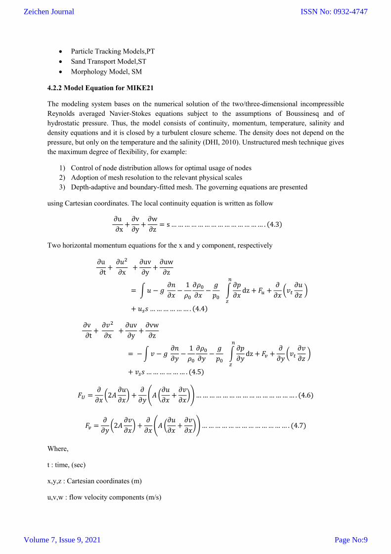
4.1.1 Governing Equations for MIKE11
MIKE11 is based on the 1D Saint-Venant equations as illustrated below:
• Continuity equation
δQ
δx+
��
��= � … … … … … … … … … … … … … … … … … … … . ( 4.1)
• Momentum equation:
��
��+
�{����}
��+ ��
��
��+ ��
�
����= 0 … … … … … … … … … … … … . (4.2)
Where Q – Discharge, (m3/s)
A – Flow area, (m2)
q – Lateral inflow, (m3/m/s)
h – Stage above datum, (m)
R – Hydraulic or resistance radius, (m)
C – Chezy resistance coefficient,
α – Momentum distribution coefficient
Zeichen Journal
Volume 7, Issue 9, 2021
ISSN No: 0932-4747
Page No:7
The four terms in the above momentum equation are local acceleration, convective acceleration,
pressure and friction. In MIKE 11, a network configuration depicts the rivers and floodplains as a
system of interconnected branches. Water levels and discharges (h) and Q) are calculated at
alternative points along the river branches as a function of time. It operates on basic information from
the river and floodplain topography to include manmade features and boundary conditions. The 6
point Abbott-Ionescu Finite Difference scheme for the dynamic, diffusive and kinematic wave
approximation is used in MIKE11. The conservation of mass i.e. continuity equation is applied
between elevation points and conservation of momentum is applied at discharge points.
4.2 About MIKE 21 Software
MIKE 21 is the leading software package for 2D modelling of hydrodynamics, waves, sediment
dynamics, water quality and ecology. It is professional software of high reliability, quality and
versatility. MIKE 21 is a modular product and includes simulation engines that are aimed at a very
wide range of applications. These include modelling of tidal flows, storm surge, advection-dispersion,
oil spills, water quality, mud transport, sand transport, harbour disturbance and wave propagation.
Apart from the simulation tools, MIKE 21 includes productivity tools to prepare input and
interpretation as well as presentation of results
MIKE 21 comprises three simulation engines:
Single Grid: the full time-dependent non-linear equations of continuity and conservation of
momentum are solved by implicit finite difference techniques with the variables defined on a
space-staggered rectangular grid.
Multiple Grids: the Multiple Grids version uses the same simulation engine and numerical
approach as the single grid version. However, it provides the possibility of refining areas of
special interest within the model area (nesting). All domains within the model area are
dynamically linked.
Flexible Mesh: is an unstructured mesh and uses a cell-centred finite volume solution
technique. The mesh is based on linear triangul
4.2.1 Flow Model with Flexible Mesh elements.
The Flow Model FM is a comprehensive modelling system for 2D surface modelelling developed by
DHI. The 2D models carry the same names as the classic DHI model version MIKE21 with an ‘FM’
added referring to the type of model grid- Flexible Mesh.The moddeling system has been developed
for complex applications within oceanographic, coastal and estuarine environments. For general
modelling system for 2D surface flows it may also be applied for studies of inland surface waters, e.g.
overland flooding and lakes or reservoirs. The FM series meets the increasing demand for realistic
representationsof nature, both with regard to look alike and to its capability to model coupled
processes, e.g. coupling between currents, waves and sediments. All models are supported by
advanced user interfaces including efficient and sophisticated tools for mesh generation, data
management, 2D visualization. etc.
The modules of the Flexible Mesh Series
DHI’s Flexible Mesh (FM) series includes the following modules:
Hydrodynamic Model, HD
Transport models,
Mud Transport Models,MT
Zeichen Journal
Volume 7, Issue 9, 2021
ISSN No: 0932-4747
Page No:8
Particle Tracking Models,PT
Sand Transport Model,ST
Morphology Model, SM
4.2.2 Model Equation for MIKE21
The modeling system bases on the numerical solution of the two/three-dimensional incompressible
Reynolds averaged Navier-Stokes equations subject to the assumptions of Boussinesq and of
hydrostatic pressure. Thus, the model consists of continuity, momentum, temperature, salinity and
density equations and it is closed by a turbulent closure scheme. The density does not depend on the
pressure, but only on the temperature and the salinity (DHI, 2010). Unstructured mesh technique gives
the maximum degree of flexibility, for example:
1) Control of node distribution allows for optimal usage of nodes
2) Adoption of mesh resolution to the relevant physical scales
3) Depth-adaptive and boundary-fitted mesh. The governing equations are presented
using Cartesian coordinates. The local continuity equation is written as follow
∂u
∂x+
∂v
∂y+
∂w
∂z= s … … … … … … … … … … … … … … . (4.3)
Two horizontal momentum equations for the x and y component, respectively
∂u
∂t+
∂��
∂x +
∂uv
∂y+
∂uw
∂z
= � � − � ��
��−
1
��
���
��−
�
�� �
��
��
�
�
dz + �� +�
�����
��
�� �
+ ��� … … … … … … . (4.4)
∂v
∂t+
∂��
∂x +
∂uv
∂y+
∂vw
∂z
= − � � − � ��
��−
1
��
���
��−
�
�� �
��
��
�
�
dz + �� +�
�����
��
�� �
+ ��� … … … … … … . (4.5)
�� =�
���2�
��
��� +
�
���� �
��
��+
��
���� … … … … … … … … … … … … … … … . (4.6)
�� =�
���2�
��
��� +
�
���� �
��
��+
��
���� … … … … … … … … … … … … … . (4.7)
Where,
t : time, (sec)
x,y,z : Cartesian coordinates (m)
u,v,w : flow velocity components (m/s)
Zeichen Journal
Volume 7, Issue 9, 2021
ISSN No: 0932-4747
Page No:9
S : magnitude of discharge due to point source
Fu, Fv : horizontal diffusion terms
h : depth above datum, (m)
ƞ(x,y) : surface elevation, (m)
g : acceleration due to gravity (m/s2)
pa(x,y,t) : atmospheric pressure (kg/m/s2)
ρo(x,y,t) : reference density of water (kg/m/s2)
The spatial discretization of the primitive equations is performed using a cellcentere finite volume
method. The spatial domain is discretized by the continuum into non-overlapping elements/cells. In
the 2-D model, the elements can be triangles or quadrilateral elements.
5. MODEL SET UP
5.1 Model Setup for MIKE11
Figure 5.1: New file dialog for Generating new MIKE 11 input file
5.1.1 Defining the River Cross-section
MIKE 11 model’s River Network file is the common link to the various MIKE 11 files. It also has an
XY coordinate system, allowing the model to import and export data to and from other software. The
River Network file allows the modeller to define the river network, reference cross-sections, and
control structures to the network and to obtain a graphical overview of model information in the
current simulation. In this case the required river network Ranga Nadi river is imported from the
Google earth and converted it to a polygon shape file using the Arc Gis 10.5 software, later open in
MIKE11 network editor. The river network file which is later digitized and defined graphically in
MIKE 11 network platform using the MIKE 11 network tools. After defining the network graphically
in MIKE11 network editor the chainage values of the network for each point can be defined
automatically.
Zeichen Journal
Volume 7, Issue 9, 2021
ISSN No: 0932-4747
Page No:10
Figure 5.2: Ranga Nadi River in MIKE11 network editor and User define chainages in
upstream and downstream points
5.1.2 Inserting River Cross-section
The cross-sections are required to be inserted both at upstream and downstream end of the branch.
The cross sections were provided for river reach at different chainage points. The x-y co-ordinates
(from left bank) were entered as raw data in the cross-section editor (Table 5.2). The raw data can be
entered using the MIKE11 cross section editor and the chainage and branch name were then
automatically transferred to the cross section editor.
Table 5.1: Cross section at various Chainage points
Sr.No,. Cross section X co-ordinates (UTM) Y co-ordinates (
UTM)
1 0 599830 3020700
2 4247.644 603380 3018600
3 9498.77 603840 3013630
4 13634.44 604700 3009670
5 22416.66 605160 3002800
6 25823.89 607680 3000860
7 29956.39 608880 2997310
8 34173.62 608840 2994120
9 38212.14 609330 2990360
Zeichen Journal
Volume 7, Issue 9, 2021
ISSN No: 0932-4747
Page No:11
Figure 5.3: Cross section profile for Ranga Nadi River
5.1.3 Boundary condition
Boundary conditions can be defined for the river reach by inserting the time-series for the upstream
and downstream boundary condition. In this case the two open boundaries were provided with the
water level at downstream and a constant inflow at upstream at cross section 38212.14m and 0m.
5.1.4 Hydrodynamic (HD) Parameter
The hydrodynamic parameters include the initial conditions of water depth and discharge, friction
coefficient and output parameter options. Present study includes the specification of both the global
and local values of roughness coefficient (Manning’s n) of the riverbed, which was the main and only
calibration parameter. Other parameters were kept at their default values. The global value for the
initial condition of water depth was kept at a low value of 0.003 m to avoid dry bed conditions.
5.1.5 Simulation Parameters
Before running the model simulation, control parameters such as simulation period, simulation time
step, data to be stored and storage time were specified. For this study the time step and computational
distance were kept as 30 min and 1000 m, for each month from March to October for, 4 years
stimulation period 2017 to 2020 respectively. After specifying all the input files the “Start” button can
be pressed and the simulation will commence. After simulation results can be viewed using MIKE
VIEW.
5.2 MIKE 21 Model Setup
5.2.1 Digital Elevation Model (DEM)
Digital Elevation Model (DEM) is a type of raster GIS layer. In a DEM, each cell of raster GIS layer
has a value corresponding to its elevation (z-values at regularly spaced intervals). DEM data files
contain the elevation of the terrain over a specified area, usually at a fixed grid interval over the “Bare
Earth”. The intervals between each of the grid points will be always referenced to some geographical
coordinate system (latitude and longitude or projected coordinate UTM (Universal Transverse
Mercator). The model studies were carried out using DEM of 30 m resolution (Figure 5.1). However,
DEM should be converted to MIKE elevation map format to be included in the model. The term
“Bathymetry” is used for the DEM as model map of MIKE. Two different types of the bathymetry
can be created for the two different types of model. MIKE 21 is single grid model and it uses grid
base bathymetry for model calculations. MIKE 21 FM is flexible mesh model and it uses triangular
mesh for model calculations. Since MIKE 21 FM was used in this study, the DEM was converted to
the flexible mesh with MIKE ZERO Mesh Generator.
Zeichen Journal
Volume 7, Issue 9, 2021
ISSN No: 0932-4747
Page No:12
Figure 5.4 Digital elevation model of the study area (Source: ArcGIS 10.3 student version
5.2.2 MIKE 21 Mesh Generation
A mesh is a representation of a larger geometric domain by smaller discrete cells. Meshes are
commonly used to compute solutions of partial differential equations and render computer graphics,
and to analyse geographical and cartographic data. A mesh partitions space into elements (or cells or
zones) over which the equations can be solved, which then approximates the solution over the larger
domain. Element boundaries may be constrained to lie on internal or external boundaries within a
model. There are two types of two-dimensional cell shapes that are commonly used. These are the
triangle and the quadrilateral. The MIKE ZERO MESH generator provides an environment for
creating, editing and presenting detailed digital 2D bathymetries. Mike zero software generates
bathymetries in a rectangular grid (dfs2) whereas the Mesh Generates bathymetry in a flexible mesh
format (mesh). The program provides the utilities for importing raw data from various external
sources (i.e. xyz grid file, xyz contour, MIKE21/MIKE 3 formatted data), or to manually create data
by using the built-in drawings tools. For this process rectified digital elevation model is converted into
a tiff file using Arc GIs 10.1 and open the Tiff file in Global Mapper to transfer it to a xyz grid
format. After starting the Mesh Generator the projection system has been specified as WGS 1984
UTM and the zone as 46 for the working area. In order to evaluate the outline of the model area all the
available scatter data were imported and the map projection for the individual xyz grid files defined
during import.
Zeichen Journal
Volume 7, Issue 9, 2021
ISSN No: 0932-4747
Page No:13
Figure 5.5 Workspace as it appears in the Mesh Generator after importing scatter with its open
boundaries
The scattered data with open boundary points are joined by using the arc tool available in the mesh
generation tool box .Total numbers of nodes are drawn and two nodes at the position (94.2737,
27.5289) and (94.25672, 27.52856) are inserted respectively, the nodes points are connected by
drawing a arc to close u the whole area. The node points and arcs on the open boundaries must be
defined by a unique integer value. These attributes are used for the model system to distinguish
between the different boundaries types in the mesh. The elements near the land boundary depends
highly on the resolution of the boundary for each vertex on the boundary line, a node will be generate.
Thus by modifying the number of vertices on the boundary line the mesh resolution will change
accordingly in the adjacent areas. After modifying the land boundary, the mesh may be generated and
smoothed in order to see the effect of the changed setup. There are generally two types of
two-dimensional cell shapes that are commonly used. These are the triangle and the quadrilateral. A
triangle mesh is a type of polygon mesh in computer graphics. It comprises a set of triangles (typically
in three dimensions) that are connected by their common edges or corners. With individual triangles,
the system operates on three vertices for every triangle. The mesh components are vertices, edges, and
triangles. In a large mesh, there could be eight or more triangles meeting at a single vertex - by
processing those vertices just once, it is possible to do a fraction of the work and achieve an identical
effect. For the mesh generation the next step is to triangulate the domain (Mesh- Generate mesh) with
maximum element area 50000m2 smallest allowable angle 30 degree and considering maximum
number of nodes 100000. The resulting mesh is shown in (Figure 5.6).
Figure 5.6: Resulting mesh after smoothing 100 times
5.2.3 Bathymetry Generation
Bathymetry is the measurement of the depth of water in oceans, rivers, or lakes. Bathymetric maps
look a lot like topographic maps, which use lines to show the shape and elevation of land features. On
topographic maps, the lines connect points of equal elevation. On bathymetric maps; they connect
points of equal depth. The initial bathymetry is created from the initial mesh by interpolating scatter
data. First the xyz-file containing the water depths from the measurements of regional lines (Data-
Manage Scatter Data -Add) is imported and Specifying the projection as UTM-46N. Now the
bathymetry values are interpolate by using the default settings for the interpolation (Mesh-
Interpolate). The Mesh Generator gives two possibilities with respect to interpolation for triangular
Zeichen Journal
Volume 7, Issue 9, 2021
ISSN No: 0932-4747
Page No:14
elements. The two possible interpolation routines are Natural Neighbour and Linear Interpolation. For
this interpolation Natural neighbour is used and extrapolation is kept constant. After the interpolation
the mesh is exported from the Mesh Generator to a mesh file. The resulting mesh can view (and edit)
in the Data Viewer.
Figure 5.7: Resulting mesh bathymetry
5.3 Mike 21 HD Flow Model Run
The Hydrodynamic Model provides the basic for computations performed in many other modules, bit
can also be used alone. It stimulates the water level variations and flows in response to a variety of
forcing functions on flood plains, in lakes, estuaries and coastal areas
Figure 5.8: The user interface of MIKE21 HD model
5.3.1 Domain
For setting up the model the first step is to specify the domain area for that the interpolate bathymetry
mesh is use as an input parameter. The Bathymetry mesh covers the whole study area. The projection
zone can be define as UTM 46N automatically.
5.3.2 Flood and Dry
For cases such as areas with tidal flats or for inland flooding, the concept of flood and dry point is
utilized by MIKE 21 as a way to deal with moving boundaries, the drying and flooding fronts. The
dry point is the minimum water level (drying depth, hdry) that a flooded cell reaches before it is taken
Zeichen Journal
Volume 7, Issue 9, 2021
ISSN No: 0932-4747
Page No:15
out of the calculations and made inactive. The water depths of the dry cells are stored and can be used
at later time step in the calculations in case more water flows to the cell. The threshold for activating a
dry cell was defined by the flooding depth, hflood. The default value for flood and dry depth are kept
as 0.1 and .005. The relationship between those two threshold parameters must be: hflood> hdry.
5.3.3 Eddy’s Viscosity
Eddy viscosity represents the loss of energy due to the creation of eddies in the water. In applications
with significant flooding and drying of the MIKE 21 grid cells, the equation of Smagorinsky is the
most suitable eddy viscosity formulation. The eddy viscosity was set as flux based according to DHI
to avoid potentially numerical instabilities. A value of 0.28 was used for the entire domain.
5.3.4 Bed Resistance
Surface resistance played a crucial part in the calibration process since it is a parameter with high
uncertainty and big influence on the result of the water level and flood extent. In the cases where the
focus of the study is a river, factors such as channel meandering, silting and scouring, size and shape
of the channel as well as suspended material and bed load are also expected to affect the value of the
coefficient. For this stimulation the bed resistance Manning’s coefficient value was kept 32m1/3/s for
the whole domain.
5.3.5 Boundary conditions
The boundary conditions represent the different inputs of parameters in the model. Boundary
conditions are usually defined by hydrographs at upstream and water levels at the downstream
boundaries of the model. For this study the boundary format is considered as varying in time but
constant along the boundary. During the calibration and verification of the model, water level series
data for Ranganadi River were used as input boundary conditions in MIKE 21 (HD) model.
5.3.6 Simulation period and Output files
The stimulation period of the HD model was set from the 1 July to the 30th of July 2017. The time
step interval is kept at 180sec covering the time steps of 12960 numbers. For the solution technique
shallow water equation was used, keeping the Time integration and space discretization at higher
order. The minimum and maximum time steps for the shallow water equation are set at 0.01 and 30
sec. Critical CFL number was kept at 0.8. After specifying all the input files the “Run” button can be
pressed and the simulation will commence. After simulation output datas for MIKE21 HD model can
be views in Area.df0, Line.dfs1 and Point.dfs format. For this present study Area.dfso and line.dfs1
output formats are considred. The output results can be saved in defined points, lines and areas.
Output from MIKE 21 Flow Model FM is typically post-processed using the Data Viewer available in
the common MIKE Zero shell. The Data Viewer is a tool for analysis and visualization of
unstructured data, e.g. to view meshes, spectra, bathymetries, result files in different format with
graphical extraction of time series and line series from plan view and import of graphical overlays.
6. RESULTS AND DISCUSSION
6.1 MIKE11 One-Dimensional Model Studies
The 1-D hydrodynamic model was run for total 4years high-magnitude flood event that occurred in
between the monsoon period of 2017 to 2020. In the model set up for the river network, 9 cross
sections were generated. Simulation of gauge and water level data was performed at different cross
Zeichen Journal
Volume 7, Issue 9, 2021
ISSN No: 0932-4747
Page No:16
sections of the selected reach of Ranga Nadi River. Manning’s coefficient of roughness (n) was used
as a model calibration parameter. The Manning value is used as n= 0.003 for this model studies. The
High order Dynamic Wave Method is used for unsteady 1D channel routing in this study. The
Non-linear Saint Venant equations are used for conservation of mass, volume, momentum and
continuity of flow. The model gives discharge at different cross section, velocity and as well as water
level profile at different locations of cross section.The results of MIKE 11 simulations were visualized
using the MIKE View software. MIKE View displays longitudinal profile animations of both stage
height and discharge resulting from a MIKE 11 unsteady simulation. It also can display stage height at
any given cross-section, as well as provide rating curves at a specified location along the river
network. MIKE View can also aid the visualization of time-series results of stage heights at
cross-section locations and time-series results of discharge at midpoints between two cross-section
locations. In this presents study, the longitudinal water level profile area shown in Scenario 1 and
Time series water profile are shown scenario 2. The Mike 11 stimulation result also gives the
hydraulic radius, discharge at each cross section h points, flow area and total flooded area for each
cross section which area shown in the scenario 3.
SCENARIO 1: Longitudinal Profile view of highest change in water level at each cross section
of river Ranga Nadi for the period 2017 and 2019
Figure 6.1 :Longitudinal water level profile for the month July 2017
Zeichen Journal
Volume 7, Issue 9, 2021
ISSN No: 0932-4747
Page No:17
Figure 6.2: Longitudinal water level profile for the month July 2019
Scenario 1 gives the longitudinal profile view of overall water level depth for the entire river cross
section and flood starting time. In the (Figure 6.1) the blue-coloured section represents water in the
river channel. The red dotted line denotes the maximum water level simulated during the period. The
dark continuous line represents the right river bank, while the dark broken represents the left one. No
flooding is experienced if all the maximum water simulated (red dotted line) does not rise above the
river banks. For the 4 year simulation period it is observed that water level was above max limit for
the month July 2017 and July 2019.
SCENARIO 2: The tabular view of water levels for each cross section and simulation period are
shown in the (Table 6.1), (Table 6.2).
Table 6.1 Water levels at each cross section for the simulation period of 2017(May to October)
SR.No. Cross sections(m)
May June July August September October
1 0 93.853 94.491 95.297 94.405 94.646 94.405 2 4247.644 93.853 94.491 95.297 94.405 94.646 94.405 3 9498.7701 93.853 94.491 95.298 94.405 94.646 94.405 4 13634.443 93.853 94.495 95.299 94.405 94.646 94.405 5 22416.660 93.863 94.495 95.297 94.405 94.648 94.404 6 25823.889 93.852 94.495 95.299 94.404 94.648 94.404 7 29956.386 93.851 94.496 95.300 94.404 94.649 94.404 8 34173.619 93.851 94.496 95.300 94.403 94.650 94.403 9 38212.140 93.850 94.500 95.300 94.400 94.650 94.400
Table 6.2: Water levels at each cross section for the simulation period 2019(May to October)
Zeichen Journal
Volume 7, Issue 9, 2021
ISSN No: 0932-4747
Page No:18
SR.No. Cross sections (m)
May June July August September October
1 0 94.120 94.350 95.095 94.890 93.320 93.930 2 4247.644 94.120 94.350 95.095 94.890 93.320 93.930 3 9498.7701 94.120 94.350 95.095 94.890 93.320 93.930 4 13634.443 94.120 94.350 95.096 94.890 93.320 93.930 5 22416.660 94.120 94.350 95.096 94.890 93.120 93.930 6 25823.889 94.120 94.350 95.097 94.890 93.120 94.120 7 29956.386 94.120 94.350 95.009 94.890 93.120 94.120 8 34173.619 94.120 94.410 95.100 94.890 93.120 94.120 9 38212.140 94.200 94.410 95.100 95.000 93.120 94.300
SCENARIO 3: The combination of all the model output values MIKE11 1D model for the entire
4 years stimulation period (2017 to 2020)
Table 6.3: MIKE11 1D model outputs for the simulation period 2017 to 2020
Sr.no
Output parameter
Simulation period
2017
2018
2019
2020
1
Maximum Water level (m)
95.300
94.801
95.10
94.604
2
Maximum Discharge(m3/s)
7.646
6.572
18.117
8.550
3
Maximum Hydraulic Depth(m)
8.504
8.135
8.536
7.989
4
Maximum Flooded Area(m2)
941183.89
900221.75
9937586.93
875233.32
5
Maximum Flow width (m)
35.53
35.130
35.59
34.61
6
Flow Area(m)
267.091
249.714
268.675
242.900
7
Bed shear stress (N/m2)
0.562
0.03
0.319
0.028
8
Maximum water level depth(m)
10.190
9.995
10.346
9.598
Results from the scenarios 3 investigation indicate that two major flood event that occurred for the
year 2017 and 2019 had flooded more areas compared to the other two flood events. The flood event
that took place on 10/7/2017 flooded total maximum 232.57 acres area and 9/07/2019 flood event
covered total maximum area of 231.68 acres. Among the all 4 years simulation period 2017 flood
event is considered as most flooding experienced event. The reason for that can be the rainfall
characteristics of the area. The combination of all the model output values MIKE11 1D model for the
entire stimulation period is shown in the table 6.3.
6.2 Two-Dimensional Model Studies
In this present paper the MIKE21 2D HD model is prepared for the Ranga Nadi river flood plain
North Lakhimpur .The Calibration simulation period of the HD model was set from the 1 July to the
30th of July 2017. The time step interval is kept at 180sec covering the time steps of 12960 numbers.
This produces a courant number of 5.1 which is a good indicator for model stability. In the first
Zeichen Journal
Volume 7, Issue 9, 2021
ISSN No: 0932-4747
Page No:19
simulation, many blow-ups occurred ending the simulations prematurely. These blow-ups came from
certain grid points where bathymetry was not well smoothed, or where the slope between two
grid-points was too steep. Then, after a few rectifications and schematizations in the bathymetry, the
simulation can end, although due to some uncertainties the stimulation ended prematurely. The
calibrated output parameters can now be viewed in area.dfsu, line.dfs1 and point.dfso format. For this
study all the output values are shown in the AREA.dfsu format below in scenario 5.
SCENERIO 4: Output values of MIKE21 HD model shown in the AREA.dfsu format for the
period 2017(July)
Figure 6.3: Change in Surface elevation and change in element area in Area.dfsu format for the
stimulation period July 2017
Figure 6.4.: Change in Wind U and V velocity in Area.dfsu format for July 2017
The Results from the scenarios 4 investigation indicate that all the output values are totally dependent
on the change in the time interval, and every time consuming, for this presents study all the output
values are recorded for each day at 3min time intervals for the highly considered flooding month July
Zeichen Journal
Volume 7, Issue 9, 2021
ISSN No: 0932-4747
Page No:20
2017.The observed output for considered stimulation period of July 2017 from the staring to the
ending of the month area discussed in a tabular format in table (6.4).
Table 6.4: Observed output result from the mike21 2D Calibration
Sr.no Output parameters Stimulation period July 2017
Starting Ending 1
Surface Elevation(m)
235.481
94.88108 2
Air pressure (Pascal)
101300
101300 3
Wind U velocity(m/s)
10
10 4
Wind V velocity(m/s)
-0.000033585
-0.000033577 5
Conveyance angle( radian)
6.283185
6.283185 6
Element Area(m2)
0.0000654
0.00100
6.2.1 Uncertainties during the Validation of the 2D model
Understanding the uncertainties is important in order to comprehend the limitation of the
methodology and the reasons that led to premature simulation. For this study a major source of
uncertainty in the floodplain model is the surface roughness. Larger the roughness, the larger will
be the uncertainty. In developing the 2D flood modelling, the accuracy is also important. However, it
is dependent on the precision of the variables used (estimation of design flow, data collection
techniques of DEMs, hydraulic modelling approach). With regards of the uncertain variables, the
approach of using the probabilistic. For this 2D model study although several corrections in the
bathymetry were made, the stimulation stops prematurely. Depending on the availability of the
historical Hydrological data, the approach of estimating the 2D modelling would be different. But for
this research there is no past data are available to validate the model with the calibration model
outputs. That’s why the 2D model failed to validated for the 2107. With regards of the uncertain
variables, the approach of using the probabilistic 2D model outputs should be deliberate and explored
further in the future.
7. CONCLUSION
A flood is an unusually high stage in a river normally the level at which the river overflows its banks
and inundates the adjoining area. The damages caused by floods are in terms of loss of lives, property
and economic loss due to disruption of economic activities are with great severity. Hence information
about the flood has to be disseminated well in advance to the people likely to be affected so that an
emergency evacuation plan may be prepared and properly implemented. In recent years MIKE 11 and
MIKE21 became more popular tool used for flood forecast-ing and 2D free surface flow modelling
due to its inherent properties. MIKE 11 has been used in hundreds of application around the world. Its
main application areas are flood analysis and alleviation design, real-time flood forecasting, dam
break analysis, optimization of reservoir and canal gate/structure operations, ecological and water
quality assessments in rivers and wetlands, sediments transport and river morphology studies,
salinity intrusion in rivers and estuaries. MIKE21 2DHydrodynamic module basically solves two
dimensional shallow water equations that are depth integrated Reynolds averaged Navier Stokes
Zeichen Journal
Volume 7, Issue 9, 2021
ISSN No: 0932-4747
Page No:21
equations. Therefore, model includes continuity, momentum, salinity, density and temperature
equations. The Results from the scenarios of MIKE11 model indicate that the two major flood event
that occurred in 2017 and 2019 had attained the highest water level and discharge on 10/07/2017 and
9/07/2017, due to which flooding had experienced in the area near the mouth of Ranga Nadi River.
The water level on 12/07/2017 raised above its maximum limit to 95.300m and during the 9/07/2019
flood water level reached to a maximum limit of 95.100m. The highest max discharge was observed
as 18.117 m3/s at the upstream side of the river for year 2019 on 11/07/2019.The area affected during
the 12/7/2020 and 9/07/2019 flood were approximately 941183.89 m2 and 9937586.93 m2
respectively, both observed to be at the upstream side of the river. The depth of water level for the
month July 2017 and July 2019 found out to be 10.19m and 10.34m respectively. Among all four
simulation period from 2017 to 2020 for the month July 2019 the depth of water level is observed to
be maximum. The other output parameters for the 4 years flood event 2017 to 2020 are given in the
(Table 6.3). This study is a good way to know about the floods probability, and the locations where
the flow will overflow. It can be also used as a risk analysis trial. For the 2D hydrodynamic model,
MIKE21 flood model is calibrated and validated for the year 2017 for the flood plain North
lakhimpur.Due to the uncertainty associated with the 2D hydrodynamic model, and unavailability of
the past hydrological data the model failed to validate for the year 2017. The output results are
discussed in table (6.4).The calibration of the 2D model results provide some valuable information
about Wind velocity, air pressure, surface elevation and element area for the high flooded month July
2017. After executing the both MIKE11 1D and MIKE 2D model one can say that MIKE-11 model is
the one which simulated the best results for this case study. The outputs from the MIKE11 1D model
are very useful since it provides quick substantial information that can be used in the decision making
progress and also as a risk analysis tool. The proposed modelling system can also use as a good way
to know about the floods probability, and the locations where the flow will overflow in the near future
years.
ACKNOWLEDGEMENT
At the very outset, I am pleased and highly honoured to express my sincere and heartfelt gratitude to
my supervisor and examiner Ms. Shaheen Akhatar Wahab, Assista Professor, Department of Civil
Engineering, The Assam Kaziranaga University, Jorhat-785006, for her kind guidance, providing
different solution and, motivation towards my master thesis. I would also like to take the opportunity
to thank Prof. (Dr.) Shwetambara Verma, Head of Department, Civil Engineering, The Assam
Kaziranga University, Jorhat-785006.
REFERENCES
[1] Akbari,G.H., and Barati,R.(2012), Comprehensive analysis of flooding in unmanaged catchments.
Proceeding of the institution of Civil Engineers-Water Management, 165(4), 229-238.
[2] Asselman, N., Bates, P., Woodhead, S., Fewtrell, T., Soares‐Frazão, S., Zech, Y., Velickovic, M.,
de Wit, A., ter Maat, J., Verhoeven, G., and Lhomme, J. (2009), Flood inundation modelling: Model
choice and proper application, Floodsite, Report‐T08‐09‐03.
[3] Bales, J. D., and Wagner, C. R. (2009), Source of uncertainty in flood inundation maps. Journal of
Flood Risk Management, 2, 139‐147
[4] Berz, G., (2000), Flood disasters: lessons from the past‐worries for the future. Proceedings of the
Institution of Civil Engineers‐Water and Maritime Engineering, 142(1), 3‐8.
Zeichen Journal
Volume 7, Issue 9, 2021
ISSN No: 0932-4747
Page No:22
[5] Blazkova, S., and Beven, K. (2009), A limits of acceptability approach to model evaluation and
uncertainty estimation in flood frequency estimation by continuous simulation: Skalka catchment,
Czech Republic. Water Resources, Research, 45, W00B16.
[6] Brandt, S. A., & Lim, N. J. (2012). Importance of river bank and floodplain slopes on the accuracy
of flood inundation mapping. In R. Murillo Muñoz (Ed.), River Flow 2012. (pp. 1015–1020). San
José, Costa Rica: CRC Press/Balkema (Taylor & Francis).
[7] Brandt, S. A., & Lim, N. J. (2016). Visualising DEM-related flood-map uncertainties using a
disparity-distance equation algorithm. In A. H. Schumann (Ed.), Proceedings of the International
Association of Hydrological Sciences (IAHS): The spatial dimensions of water management
Redistribution of benefits and risks (pp. 153–159).
[8] Cook, A., and Merwade, V. (2009), Effect of topographic data, geometric configuration and
modelling approach on flood inundation mapping. Journal of Hydrology, 377 (1‐2), 131‐142.
[9] Di Baldassarre, G., Schumann G., Bates, P. D., Freer, J. E., and Beven, K. J. (2010), Flood‐plain
mapping: a critical discussion of deterministic and probabilistic approaches. Hydrological Sciences
Journal.
[10] DHI 2007,MIKE 21 and MIKE FLOOD user and reference manuals.
[11] Leandro, J. (2008). Advanced modelling of flooding in urban areas: integrated 1D/1D and 1D/2D
Models. PhD thesis, University of Exter.
[12] MIKE 11 - A modeling system for rivers and channels, Short introduction and tutorial, DHI,
Horsholm, Denmark.
Zeichen Journal
Volume 7, Issue 9, 2021
ISSN No: 0932-4747
Page No:23