Development of a 0.2 % High-Speed Dry Piston Prover · PDF file5.1. Flow-Independent...

Development of a 0.2 %High-Speed Dry Piston Prover

Harvey PaddenBios International Corporation

10 Park Place, Butler, NJ 07405, U.S.A. Phone: 973.492.8400 • FAX: 973.492.8270

[email protected] • www.biosint.com

Presented at 2003 Measurement Science Conference

2Bios International Corporation • 10 Park Place, Butler, NJ, USA 07405Phone: 973.492.8400 • Toll Free: 800.663.4977 • Fax: 973.492.8270 • www.biosint.com

Abstract ..........................................................................................................................................................1

1. Introduction ................................................................................................................................................1

2. Piston Prover Operating Principles and Variations .....................................................................................2

3. Dynamic Considerations for Standardization ..............................................................................................4

3.1 Pressure ..................................................................................................................................................... 4

3.2 Temperature ............................................................................................................................................... 6

4. Uncertainty Contributions ...........................................................................................................................6

4.1 Repeatability of Readings (Piston oscillations, rocking, detector trip point, quantization) ..................... 7

4.2 Leakage ...................................................................................................................................................... 7

4.3 Pressure Standardization .......................................................................................................................... 8

4.4 Temperature Standardization .................................................................................................................... 9

4.5 Measured Piston Diameter ...................................................................................................................... 10

4.6 Effective Piston Diameter ....................................................................................................................... 10

4.7 Measurement Length Calibration ............................................................................................................ 12

4.8 Thermal Expansion .................................................................................................................................. 12

4.9 Measurement Length Drift ...................................................................................................................... 12

4.10 Time Base Calibration............................................................................................................................ 14

4.11 Piston Rocking ....................................................................................................................................... 14

5. Uncertainty Statements ............................................................................................................................ 14

5.1. Flow-Independent Uncertainty ............................................................................................................... 14

5.2. Flow-Dependent Uncertainty .................................................................................................................. 14

5.3 Total Uncertainty ...................................................................................................................................... 15

6. Conclusions and Observations .................................................................................................................. 17

Figure 1 - Idealized Automatic Piston Prover .................................................................................................3

Figure 2 - Practical Piston Prover ...................................................................................................................4

Figure 3 – Intra-Cycle Cell Pressure ...............................................................................................................5

Figure 4 – Dual Pressure Transducer Variant .................................................................................................8

Figure 5 – Thermistor Drift .............................................................................................................................9

Figure 6 - Adaptive Detection ....................................................................................................................... 13

Figure 7 - Standardized ML-800 Small Cell Expanded Uncertainty (2X) ....................................................... 16

Figure 8 - Standardized ML-800 Medium Cell Expanded Uncertainty (2X) .................................................... 16

Figure 9 - Standardized ML-800 Large Cell Expanded Uncertainty (2X) ....................................................... 17


AbstractThere has been a long-standing need for economical, high-speed primary standards for use in the manufacture and recalibration of mass flow controllers (MFCs) and mass flow meters in the 5 sccm to 50 slm flow range. It is especially desirable to obtain a dynamic range (turndown) greater than the 10:1 ratio typical of existing devices.

Exhibiting turndown ranges of hundreds to one, the provers described here use a clearance seal between a graphite piston and borosilicate glass cylinder. They are small, portable, fast, and contain no toxic materials. Reading cycle time is on the order of seconds. Used in conjunction with a stable flow generator, they are also very suitable for calibration of flow meters.

We have previously reported on clearance-sealed volumetric Laboratory Master Provers with an expanded uncertainty approximately 0.07% [1]. These later formed the basis of the 0.4% ML-500 system [2], with temperature and absolute pressure transducers added to allow standardization of the readings.

The prover described here is intended for use in the 0.2% range. The production version of the ML-500 was used as a starting point. The cylinder was lengthened to increase the volumetric repeatability, but the biggest improvements were in the standardization system. A special high-accuracy, high-speed transducer system was added to permit unique dynamic standardization techniques to be developed.

This paper is necessarily an uncertainty analysis as well as a description of our design. Although we designed for 0.2% expanded uncertainty (at 2X), the analysis that follows shows typical single-reading results of better than 0.85% to 0.12%, depending on flow.

That being said, this is a preliminary analysis of an experimental system. We will now build several units for better statistical verification of the reproducibility and for inter-laboratory, inter-methodology testing. We have great confidence that the subsequent uncertainty analysis will confirm that our goal of 0.2% has been met.

1.0 IntroductionThe trend in MFC development is toward more precise devices with larger turndown ranges. To calibrate an MFC to 1.0% expanded uncertainty with high yield, a calibrator of 0.25% (or better) accuracy is required. If we are to eventually proceed to 0.5% MFCs, a 0.125% calibrator will be needed. The use of primary calibrators with high turndown ratios will minimize both the initial expenditure for such precise devices (less devices are required when they exhibit high turndown) and the cost of maintaining the devices in calibration (less calibrations need to be performed).

We began our work in this area with the same basic clearance-sealed dry piston design used in our prior commercial DryCal models. Approximately 20,000 of these simple devices have been produced over the last 11 years. Used principally for environmental air sampler calibration, these devices are of 1% volumetric and 1.4% standardized expanded uncertainties. Although far from the accuracy required of our new designs, they supplied an extensive knowledge base from which to begin our work.

We have retained the modular concept used in our earlier machines: Three sizes of cells are used interchangeably with a universal base. In the new designs, each cell contains everything that must be calibrated, except for the crystal time base. The base, in turn, contains all of the control and data-processing functions. These include data logging, communications, interval operation and other features.

We began by producing laboratory master provers using an extension of the eventual commercial (DryCal ML-500) design. We fabricated two each of three sizes of measuring cells for use with a common control base. We calibrated the cells by dimensional means. We then performed a rigorous uncertainty analysis stating that our primary laboratory master volumetric provers have an expanded (2X) uncertainty of approximately 0.07% [1].


Meanwhile, we proceeded to develop our ML-500 standardized primary flow calibrator. Using the same basic design as the laboratory master provers, these devices have a shorter measuring path and include standardization using internal temperature and pressure sensors

The temperature sensor is located on the centerline of the measuring cylinder and directly below it. Because the devices are fast and automatic, we were able to easily collect extensive statistically valid data for each flow we tested. Again, we performed a rigorous uncertainty analysis of the ML-500 devices. The analysis showed that our goal of 0.5% expanded uncertainty was conservative: In most of the flow regime, 0.35% to 0.4% was the result [2].

The next logical step was to evolve the 0.07% laboratory master provers into field-ready calibrators in the 0.2% range. Using direct dimensional calibration, we had the laboratory master provers’ volumetric accuracy as a starting point. However, even in the ML-500 series, the standardization process limited our accuracy. To reduce the uncertainty of our pressure and temperature sensors to acceptable levels, multipoint dynamic calibration methods were developed and evaluated.

In this work, we will present design details and our uncertainty analysis of these new 0.2% standardized devices, which we will call the DryCal ML-800 series. We will also include an update on our progress with inter-laboratory comparisons.

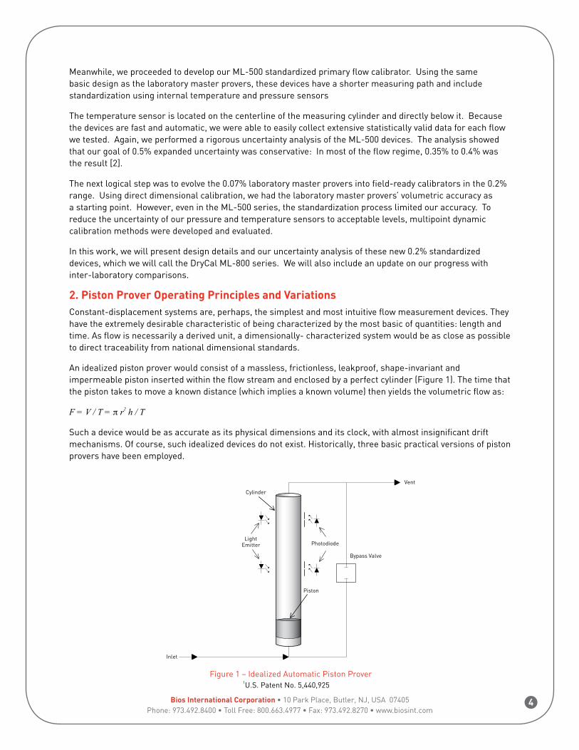
2. Piston Prover Operating Principles and Variations Constant-displacement systems are, perhaps, the simplest and most intuitive flow measurement devices. They have the extremely desirable characteristic of being characterized by the most basic of quantities: length and time. As flow is necessarily a derived unit, a dimensionally- characterized system would be as close as possible to direct traceability from national dimensional standards.

An idealized piston prover would consist of a massless, frictionless, leakproof, shape-invariant and impermeable piston inserted within the flow stream and enclosed by a perfect cylinder (Figure 1). The time that the piston takes to move a known distance (which implies a known volume) then yields the volumetric flow as:

F = V / T = π r2 h / T

Such a device would be as accurate as its physical dimensions and its clock, with almost insignificant drift mechanisms. Of course, such idealized devices do not exist. Historically, three basic practical versions of piston provers have been employed.

Bypass Valve

Vent

Inlet

Cylinder

Piston

LightEmitter Photodiode

Figure 1 – Idealized Automatic Piston Prover1U.S. Patent No. 5,440,925


The DryCal clearance-sealed prover uses a piston and cylinder fitted so closely that the viscosity of the gas under test results in a leakage small enough to be insignificant. For reasonable leakage rates, such a gap must be approximately 10 microns. As a practical matter, the piston and cylinder are made of graphite and borosilicate glass because of their low, matched temperature coefficients of expansion and low friction .

An uncertainty analysis for such an instrument has unique considerations. The static uncertainties must be evaluated in a manner similar to that used for conventional provers. In addition, though, dynamic uncertainties resulting from a significant underdamped piston mass, the effects of inventory volume and leakage must be assessed. Finally, standardization must be applied for most uses (Figure 2), with particular attention paid to dynamic accuracy of the standardizing parameters.

Bypass Valve

Vent

TemperatureTransducer

Dead Volume

Inlet Filter

Inlet

Cylinder

Piston

15 PSI AbsoluteTransducer

LightEmitter

Photodiode/ Collimator

Figure 2 - Practical Piston Prover

3. Dynamic Considerations for StandardizationTraditionally, standardization of constant-volume devices has been treated in a static manner. Pressure and temperature were measured in the inlet piping by low-speed transducers, accepting the resultant uncertainties. Yet, correlation of the average inlet temperature to that of the measured gas was always questionable.

More recently, evidence has been presented of dynamic pressure variations in bell provers [3], as well as in dry piston provers. We cannot treat standardization in a static manner. Following are our initial efforts to achieve dynamic standardization:

3.1 PressureThe DryCal is intrinsically a volumetric prover. As a piston prover is potentially subject to accelerative, oscillatory and piston-jamming effects, internal dynamic pressures must be measured to minimize uncertainty. An oscilloscope trace of the internal pressure of a typical DryCal is shown in Figure 3. Note that the timed interval begins near the center of the trace, and that the vertical scale is approximately 1.2 mbar/cm.


Measurement Science Conference 2003 5

Figure 3 – Intra-Cycle Cell Pressure

To a first order, pressure only needs to be measured at the beginning and end of the timed

measurement period. From the Ideal Gas Law, flow will be given by:

Where:

F = Flow

FI = Uncorrected flow

PA = Ambient (or standardizing) pressure

P1 = Pressure at start of timed period

P2 = Pressure at end of timed period

VD = Dead volume

VM = Measured volume

Uncorrected, the measured volume contains an error equal to the difference in internal pressure

at the start and the end of the measuring period, amplified by the ratio of dead volume to

measurement volume, as well as that of the pressure within the cylinder at the end of the timed

period. The DryCal is a high-speed device. As a result, the internal pressure changes rapidly and

can significantly affect measurement uncertainty.

For this reason, true dynamic pressure measurement has been incorporated in this prover. Once

the dynamic pressure correction is determined, it is used to correct for the potential uncertainty,

thereby enhancing the instrument’s accuracy. With knowledge of the dead volume, which will be

constant for a given instrument design using a specified amount of external dead volume, the

uncertainty resulting from the dynamic pressure differences can be minimized. This approach’s


To a first order, pressure only needs to be measured at the beginning and end of the timed measurement period. From the Ideal Gas Law, flow will be given by:



To a first order, pressure only needs to be measured at the beginning and end of the timed

measurement period. From the Ideal Gas Law, flow will be given by:

Where:

F = Flow





VD = Dead volume


Uncorrected, the measured volume contains an error equal to the difference in internal pressure

at the start and the end of the measuring period, amplified by the ratio of dead volume to

measurement volume, as well as that of the pressure within the cylinder at the end of the timed

period. The DryCal is a high-speed device. As a result, the internal pressure changes rapidly and

can significantly affect measurement uncertainty.

For this reason, true dynamic pressure measurement has been incorporated in this prover. Once

the dynamic pressure correction is determined, it is used to correct for the potential uncertainty,

thereby enhancing the instrument’s accuracy. With knowledge of the dead volume, which will be

constant for a given instrument design using a specified amount of external dead volume, the

uncertainty resulting from the dynamic pressure differences can be minimized. This approach’s

Where:

F = Flow





VD = Dead volume


Uncorrected, the measured volume contains an error equal to the difference in internal pressure at the start and the end of the measuring period, amplified by the ratio of dead volume to measurement volume, as well as that of the pressure within the cylinder at the end of the timed period. The DryCal is a high-speed device. As a result, the internal pressure changes rapidly and can significantly affect measurement uncertainty.


For this reason, true dynamic pressure measurement has been incorporated in this prover. Once the dynamic pressure correction is determined, it is used to correct for the potential uncertainty, thereby enhancing the instrument’s accuracy. With knowledge of the dead volume, which will be constant for a given instrument design using a specified amount of external dead volume, the uncertainty resulting from the dynamic pressure differences can be minimized. This approach’s effectiveness is limited by the pressure measurement’s total accuracy (including secondary uncertainties such as synchronicity and quantization) and the dead volume’s accuracy. So far, preliminary experimental results show a significant reduction in the standard deviation of constant-flow readings. We will conduct extensive statistical work in the future.

3.2 TemperatureOne of the largest potential error sources in standardization of provers is in the measurement of a truly representative standardization temperature. If the incoming flow stream varies in temperature from that of the prover, we must find means of assessing the effective measurement temperature.

Our best solution is measurement of both the inlet flow stream and, most importantly, the temperature of the slug of gas ejected from the cylinder after measurement. Since the ejection time is generally less than a second, the ejected slug will tend to be representative of the measurement temperature.

Now our problem is similar to the pressure standardization dilemma: We need a dynamic temperature measurement technique of very high speed and very high accuracy. To this end, we employed near-microscopic thermistors (about 100 micron diameter) at the end of a probe such that the still-air time constant was approximately 100 microseconds. We located the thermistor on the centerline of the cylinder and immediately beneath it.

With a combined uncertainty of 136 ppm, we have achieved our objective of a high-accuracy, stable, high-speed temperature transducer. Initially, we will standardize our readings to the temperature of the just-measured, ejected slug of gas. Eventually, we plan to measure the error resulting from the difference in inlet and instrument temperatures using percent uncertainty per degree of temperature difference (differential temperature) as a figure of merit.

Since the gas in ejected slug can be expected to have moved closer to the instrument temperature than it was during the measurement period, we expect that a blend of inlet (T

IN) and ejected (T

OUT) gas temperatures can be

used to achieve the highest rejection of differential temperature. There will be an optimum, experimentally determined, α for each flow in each size cell, using a standardizing temperature (T

EFFECTIVE) calculated as:

TEFFECTIVE = α TIN + (1 - α) T

OUT

Future work will include determining α and the rejection ratio. Our objective will be numerically quantifying uncertainty to include field applications where the inlet temperature is significantly different from that of the instrument.

4. Uncertainty ContributionsIt was not necessary to measure all of the uncertainty sources previously described. Many of them affect only repeatability. As these are automatic high-speed provers, it was simple to collect adequate statistical data to include them in Type A analysis. However, as the type A repeatability data was scales for the differing measurement paths of these devices, we will treat all readings as type AB or Type B.


4.1 Repeatability of Readings (Piston oscillations, rocking, detector trip point, quantization)

Extensive statistical data was collected for Type A analysis of the earlier ML-500 provers. We tested several of each size cell, taking 100 readings at each of 5 flows logarithmically spaced throughout the cells’ ranges. We then calculated the standard deviation of each flow rate’s 100 readings for each measurement point. Again, for conservatism, no attempt was made to remove flow generator and room temperature effects from the data. We averaged the readings for each flow point for each cell. Since we have yet to conduct the same level of Type A data collection for the ML-800, we used a type AB approach to estimate the ML-800 repeatability. We divided the ML-500 data by the ratio of ML800/ML-500 measurement path lengths (Table 1). The resulting uncertainties are shown in Table 2.

Table 1– ML-500/ML-800 Measurement Path Lengths

Measurement Path Lengths (inches)

Small Cell Medium Cell Large Cell

ML-500 ML-800 ML-500 ML-800 ML-500 ML-800

2.4 5.0 2.0 4.0 1.5 4.0

Table 2– ML-800 Prover Repeatability (Type AB)

Measurement Path Lengths (inches)

Small Cell Medium Cell Large Cell

Flow Rate (ccm)

Observed ML-500 u

(ppm)

Projected ML-800 u

(ppm)

Flow Rate (ccm)

Observed ML-500 u

(ppm)

Projected ML-800 u

(ppm)

Flow Rate (ccm)

Observed ML-500 u

(ppm)

Projected ML-800 u

(ppm)

250 650 312 50 730 365 250 710 266

1000 830 398 190 470 235 1000 350 131

3500 520 250 690 450 225 3500 290 109

13300 760 365 2600 470 235 13300 390 146

50000 470 226 9000 470 235 50000 980 368

4.2 Leakage Leakage will limit the instrument’s accuracy at very low flows. The instrument is tested for piston leakage by raising the piston to the topmost position, sealing the inlet and timing the passage of the piston from the upper sensor to the lower sensor. The instrument then calculates flow rate by dividing the subtended volume by the time.

The leakage is, of course, very significant in determining the lower flow limit of the cells. For this reason, all ML-800 cells are calibrated for leakage, with the average leakage value added to each reading as a tare value. Statistical tests of leakage repeatability exhibited a standard deviation of 12 percent. Therefore, 12 percent of the leakage value divided by the flow is used as a flow-dependent uncertainty. For the small, medium and large cells, these uncertainties are 0.006, 0.01 and 0.12 ccm.

4.3 Pressure StandardizationIn order to meet our requirements for total measurement error, the pressure transducer must be of an accuracy level normally associated with resonant transducers. Yet, we need the high-speed response characteristic of a silicon strain-gauge transducer to measure actual intra-reading pressure and to apply our dynamic pressure correction technique.


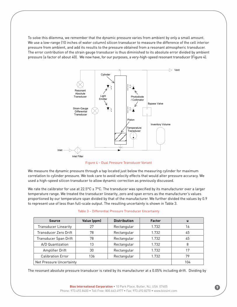
To solve this dilemma, we remember that the dynamic pressure varies from ambient by only a small amount. We use a low-range (10 inches of water column) silicon transducer to measure the difference of the cell interior pressure from ambient, and add its results to the pressure obtained from a resonant atmospheric transducer. The error contribution of the strain gauge transducer is thus diminished to its absolute error divided by ambient pressure (a factor of about 40). We now have, for our purposes, a very-high-speed resonant transducer (Figure 4).


a flow-dependent uncertainty. For the small, medium and large cells, these uncertainties are

0.006, 0.01 and 0.12 ccm.

4.3 Pressure Standardization

In order to meet our requirements for total measurement error, the pressure transducer must be of

an accuracy level normally associated with resonant transducers. Yet, we need the high-speed

response characteristic of a silicon strain-gauge transducer to measure actual intra-reading

pressure and to apply our dynamic pressure correction technique.

To solve this dilemma, we remember that the dynamic pressure varies from ambient by only a

small amount. We use a low-range (10 inches of water column) silicon transducer to measure

the difference of the cell interior pressure from ambient, and add its results to the pressure

obtained from a resonant atmospheric transducer. The error contribution of the strain gauge

transducer is thus diminished to its absolute error divided by ambient pressure (a factor of about

40). We now have, for our purposes, a very-high-speed resonant transducer Figure 4).

.

Figure 4 – Dual Pressure Transducer Variant

We measure the dynamic pressure through a tap located just below the measuring cylinder for

maximum correlation to cylinder pressure. We took care to avoid velocity effects that would

alter pressure accuracy. We used a high-speed silicon transducer to allow dynamic correction as

previously discussed.

We rate the calibrator for use at 22.5°C ± 7°C. The transducer was specified by its manufacturer

over a larger temperature range. We treated the transducer linearity, zero and span errors as the

manufacturer’s values proportioned by our temperature span divided by that of the manufacturer.

Figure 4 – Dual Pressure Transducer Variant

We measure the dynamic pressure through a tap located just below the measuring cylinder for maximum correlation to cylinder pressure. We took care to avoid velocity effects that would alter pressure accuracy. We used a high-speed silicon transducer to allow dynamic correction as previously discussed.

We rate the calibrator for use at 22.5°C ± 7°C. The transducer was specified by its manufacturer over a larger temperature range. We treated the transducer linearity, zero and span errors as the manufacturer’s values proportioned by our temperature span divided by that of the manufacturer. We further divided the values by 0.9 to represent use of less than full-scale output. The resulting uncertainty is shown in Table 3.

Table 3 – Differential Pressure Transducer Uncertainty

Source Value (ppm) Distribution Factor u

Transducer Linearity 27 Rectangular 1.732 16

Transducer Zero Drift 78 Rectangular 1.732 45

Transducer Span Drift 78 Rectangular 1.732 45

A/D Quantization 13 Rectangular 1.732 8

Amplifier Drift 30 Rectangular 1.732 17

Calibration Error 136 Rectangular 1.732 79

Net Pressure Uncertainty 104

The resonant absolute pressure transducer is rated by its manufacturer at ± 0.05% including drift. Dividing by


0.9 as above and by 1.732 to calculate the uncertainty of a rectangular distribution, u = 321 ppm.

4.4 Temperature StandardizationWe designed the circuit so that the self-heating of the probe would be insignificant with respect to our required accuracy. We then amplified the output with a precision instrumentation amplifier so that A/D quantization would be minimal.

We fitted the in-circuit voltage results to the data at several points over the design temperature range of 15 °C to 30 °C. Using a second-order polynomial (easy to program into the instrument’s microcontroller), we were able to get a fit that resulted in very little error.

Finally, we measured the drift of ten probes over a one-month period, aging the devices at 200 °C (Figure 5). This drift should far exceed the drift over a one-year period at room temperature.


We further divided the values by 0.9 to represent use of less than full-scale output. The resulting

uncertainty is shown in Table 3.

Table 3 – Differential Pressure Transducer Uncertainty

Source Value (ppm) Distribution Factor u

Transducer Linearity 27 Rectangular 1.732 16

Transducer Zero Drift 78 Rectangular 1.732 45

Transducer Span Drift 78 Rectangular 1.732 45

A/D Quantization 13 Rectangular 1.732 8

Amplifier Drift 30 Rectangular 1.732 17

Calibration Error 136 Rectangular 1.732 79

Net Pressure Uncertainty 104

The resonant absolute pressure transducer is rated by its manufacturer at ± 0.05% including drift.

Dividing by 0.9 as above and by 1.732 to calculate the uncertainty of a rectangular distribution, u

= 321 ppm.

4.4 Temperature Standardization

We designed the circuit so that the self-heating of the probe would be insignificant with respect

to our required accuracy. We then amplified the output with a precision instrumentation

amplifier so that A/D quantization would be minimal.

We fitted the in-circuit voltage results to the data at several points over the design temperature

range of 15 °C to 30 °C. Using a second-order polynomial (easy to program into the

instrument’s microcontroller), we were able to get a fit that resulted in very little error.

Finally, we measured the drift of ten probes over a one-month period, aging the devices at 200

°C (Figure 5). This drift should far exceed the drift over a one-year period at room temperature.

Figure 5 – Thermistor Drift Figure 5 – Thermistor Drift

The combined results are contained in Table 4, with the total error remaining quite small.

Table 4 – Thermistor Uncertainty

SourceWorst Case Error

(ppm)Divisor u (ppm)

Curve Fit 77 1.732 44

Quantization 69 1.732 40

Self-Heat 79 1.732 46

Calibration 100 1.732 58

Drift 170 1.732 98

Net 136


4.5 Measured Piston Diameter The main precaution to be observed in measuring the piston diameter is to avoid deflection of the graphite piston by a measuring device. To avoid this problem, diameter is measured with a laser micrometer. Several readings are averaged to enhance accuracy.

The average piston diameter was measured using a laser micrometer. An accredited laboratory measured three diameters at 120-degree intervals at distances of one third and two thirds of the piston’s height from one edge. The six readings were averaged to obtain the piston diameter. The expanded uncertainty stated by the measuring laboratory was 40 microinches.

Assuming a coverage factor of two, the uncertainty of the readings is 0.51 microns. Dividing by the piston diameters, we obtain uncertainties of 16, 6 and 33 ppm for the small, medium and large provers respectively. Since the volume is affected by the square of the diameter, the sensitivity factor is 2.

4.6 Effective Piston Diameter This subject was analyzed in detail in our previous publication [1]. The following is a synopsis:

Direct measurement of the inside diameter of small cylinders over a relatively large distance is very difficult. For this reason, we use the instrument’s internal self-test of the piston’s leakage rate, the piston’s weight and the viscosity of gas to calculate the maximum cylinder inner diameter using the Poiseuille-Couette equations.

The aspect ratio of the gap is over 1000:1, so we can safely assume the flow within the gap to be laminar. Therefore, we know the effective diameter to be that of the piston plus the gap (½ of the gap X 2).

However, we cannot state with absolute certainty what the effective piston diameter is. Experimental data shows that the piston touches the cylinder tangentially during leakage tests. We use that condition as our nominal case.

We can conservatively estimate the maximum effective diameter to be that of an elliptical piston of such eccentricity that it touches the cylinder at two points, but which yields the same leakage as the nominal case. Taking a ratio of the two yields our maximum effective diameter. Because the eccentricities are so small, the results are equally valid for an eccentric cylinder.

With similar reasoning, we can find the effective diameter for a tapered cylinder. The limit case is a cylinder that touches the entire piston circumference at one end, with the piston touching tangentially at all other points. This yields our minimum case.

We calibrate the instrument to a diameter between the tapered limit case and the elliptical limit case. Then, for conservatism, we can assume a maximum error of half the difference between the two cases with a u-shaped probability distribution. The effective piston diameter is the mean measured diameter plus one half of the annular gap as calculated by [1]:


as the nominal case. Taking a ratio of the two yields our maximum effective diameter. Because

the eccentricities are so small, the results are equally valid for an eccentric cylinder.

With similar reasoning, we can find the effective diameter for a tapered cylinder. The limit case

is a cylinder that touches the entire piston circumference at one end, with the piston touching

tangentially at all other points. This yields our minimum case.

We calibrate the instrument to a diameter between the tapered limit case and the elliptical limit

case. Then, for conservatism, we can assume a maximum error of half the difference between the

two cases with a u-shaped probability distribution. The effective piston diameter is the mean

measured diameter plus one half of the annular gap as calculated by [1]:

Where:

D = Effective piston diameter

Dm = Measured piston diameter

F = Leakage flow rate

µ = Viscosity of air

h = Piston height

w = Piston weight

g = 980.7 cm/sec2

As the limit cases of taper and eccentricity cannot coexist, it is conservative to use a u-shaped

distribution. Uncertainty is then:

Effective piston diameter uncertainties are found in Table 5. Since the volume is affected by the

square of the diameter, the sensitivity factor is 2.

Table 5 - Effective Diametric Uncertainties

Diameter

(cm)

Annular Gap

(microns)

Max Error

(ppm)

Factor

(U-shaped)

u

(ppm)

0.95 7.3 772 2.121 364

2.4 8.4 352 2.121 166

4.44 11.8 266 2.121 125

Where:





μ = Viscosity of air

h = Piston height

w = Piston weight

g = 980.7 cm/sec2

As the limit cases of taper and eccentricity cannot coexist, it is conservative to use a u-shaped distribution. Uncertainty is then:


as the nominal case. Taking a ratio of the two yields our maximum effective diameter. Because

the eccentricities are so small, the results are equally valid for an eccentric cylinder.

With similar reasoning, we can find the effective diameter for a tapered cylinder. The limit case

is a cylinder that touches the entire piston circumference at one end, with the piston touching

tangentially at all other points. This yields our minimum case.

We calibrate the instrument to a diameter between the tapered limit case and the elliptical limit

case. Then, for conservatism, we can assume a maximum error of half the difference between the

two cases with a u-shaped probability distribution. The effective piston diameter is the mean

measured diameter plus one half of the annular gap as calculated by [1]:

Where:




µ = Viscosity of air

h = Piston height

w = Piston weight

g = 980.7 cm/sec2

As the limit cases of taper and eccentricity cannot coexist, it is conservative to use a u-shaped

distribution. Uncertainty is then:

Effective piston diameter uncertainties are found in Table 5. Since the volume is affected by the

square of the diameter, the sensitivity factor is 2.


Diameter

(cm)

Annular Gap

(microns)

Max Error

(ppm)

Factor

(U-shaped)

u

(ppm)

0.95 7.3 772 2.121 364

2.4 8.4 352 2.121 166

4.44 11.8 266 2.121 125

Effective piston diameter uncertainties are found in Table 5. Since the volume is affected by the square of the diameter, the sensitivity factor is 2.


Diameter (cm)

Annular Gap (microns)

Max Error (ppm)

Factor (U-shaped)

u (ppm)

0.95 7.3 772 2.121 364

2.4 8.4 352 2.121 166

4.44 11.8 266 2.121 125

4.7 Measurement Length CalibrationThe length of the timed stroke is determined by measuring the location optical detectors using a depth micrometer to move the piston. The location of each detector was measured separately. A number of readings were taken for each detector. Each reading reproduced the others within the digital micrometer’s resolution of 0.0001 inches. Including the micrometer’s rated accuracy and dividing by 1.732 for a rectangular distribution, we calculated the uncertainties of Table 6. The sensitivity factor is 1.

Table 6 – Measurement Length Calibration Uncertainties

Size DetectorTolerance (micro in.)

Distance (inches)

u (ppm)

S Lower 105 5 12

S Upper 115 5 13

M Lower 105 4 15

M Upper 115 4 17

L Lower 106 4 15

L Upper 56 4 8


The measurement length should be calibrated using the most representative method possible. The calibration is performed once the entire measuring cell is fabricated. The piston is positioned using a depth micrometer. The trip points actually detected by the mating optics and electronics are then used to determine the stroke length and its reproducibility.

4.8 Thermal ExpansionThe graphite piston and the borosilicate glass cylinder have similar thermal coefficients of expansion of 7 ppm/K. Expansion is in three dimensions, so the sensitivity factor is 3. Over our temperature range of 7K, allowing for three degrees of freedom and for a rectangular distribution, we have a resulting uncertainty of 85 ppm.

4.9 Measurement Length DriftCollimating slits attached to the glass cylinder’s exterior mask the optical detectors. The effective width of the sensing slit is the actual slit width increased by the image of the emitter at the slit, reduced by any adaptive enhancement. The initial center-to-center spacing of the slits is a relatively straightforward measurement. However, significant potential uncertainty can arise from the position at which the sensor activates with respect to the slit. We must take into account the actual detector slit width, along with the size of the emitter’s optical image at the detector slit.

Calibration based upon direct measurement of the distances at which the piston is detected can eliminate these uncertainties, but there is potential for significant drift from other sources:

• Light output of the emitters can change with age, temperature and voltage.

• Detector sensitivity can change with temperature and age.

• Ambient light levels can change.

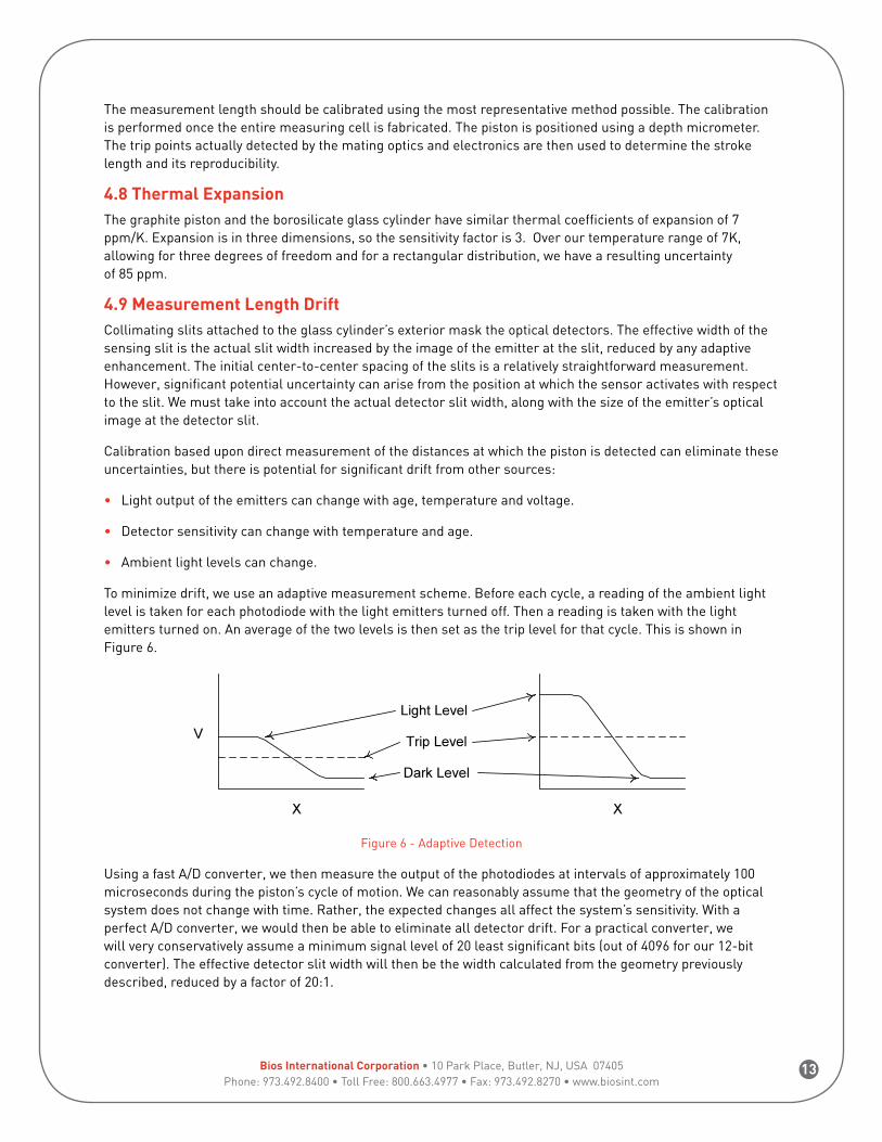
To minimize drift, we use an adaptive measurement scheme. Before each cycle, a reading of the ambient light level is taken for each photodiode with the light emitters turned off. Then a reading is taken with the light emitters turned on. An average of the two levels is then set as the trip level for that cycle. This is shown in Figure 6.


To minimize drift, we use an adaptive measurement scheme. Before each cycle, a reading of the

ambient light level is taken for each photodiode with the light emitters turned off. Then a reading

is taken with the light emitters turned on. An average of the two levels is then set as the trip level

for that cycle. This is shown in Figure 6.

Figure 6 - Adaptive Detection

Using a fast A/D converter, we then measure the output of the photodiodes at intervals of

approximately 100 microseconds during the piston’s cycle of motion. We can reasonably assume

that the geometry of the optical system does not change with time. Rather, the expected changes

all affect the system’s sensitivity. With a perfect A/D converter, we would then be able to

eliminate all detector drift. For a practical converter, we will very conservatively assume a

minimum signal level of 20 least significant bits (out of 4096 for our 12-bit converter). The

effective detector slit width will then be the width calculated from the geometry previously

described, reduced by a factor of 20:1.

In addition to the measurement length uncertainty, we must also estimate the drift of

measurement length with changes over time in sensor efficiency and emitter output. Although we

are using an adaptive detection scheme, its effectiveness is limited by quantization of the A/D

converter. This, in turn, reduces the geometric uncertainty by a factor of ±" bit divided by the

number of bits difference between the light and dark levels, with a rectangular distribution.

With our 4096 bit A/D converter, it is simple to assure that we have at least 20 bits of signal.

This will reduce the geometric piston location uncertainty by a factor of 40:1, with a rectangular

distribution. The individual uncertainty is multiplied by the square root of two to represent the

two independent detectors. The resulting uncertainties are shown in Table 7.

Table 7 - ML-800 Detector Drift Uncertainties

Size

Slit Image

(inches)

Separation (inches)

Variation (ppm)

u

Total (ppm)

S 0.014 5 135 110

M 0.014 4 169 138

L 0.0013 4 158 129

Figure 6 - Adaptive Detection

Using a fast A/D converter, we then measure the output of the photodiodes at intervals of approximately 100 microseconds during the piston’s cycle of motion. We can reasonably assume that the geometry of the optical system does not change with time. Rather, the expected changes all affect the system’s sensitivity. With a perfect A/D converter, we would then be able to eliminate all detector drift. For a practical converter, we will very conservatively assume a minimum signal level of 20 least significant bits (out of 4096 for our 12-bit converter). The effective detector slit width will then be the width calculated from the geometry previously described, reduced by a factor of 20:1.


In addition to the measurement length uncertainty, we must also estimate the drift of measurement length with changes over time in sensor efficiency and emitter output. Although we are using an adaptive detection scheme, its effectiveness is limited by quantization of the A/D converter. This, in turn, reduces the geometric uncertainty by a factor of ±½ bit divided by the number of bits difference between the light and dark levels, with a rectangular distribution.

With our 4096 bit A/D converter, it is simple to assure that we have at least 20 bits of signal. This will reduce the geometric piston location uncertainty by a factor of 40:1, with a rectangular distribution. The individual uncertainty is multiplied by the square root of two to represent the two independent detectors. The resulting uncertainties are shown in Table 7.

Table 7 - ML-800 Detector Drift Uncertainties

SizeSlit Image

(inches)Separation

(inches)Variation

(ppm)u Total (ppm)

S 0.014 5 135 110

M 0.014 4 169 138

L 0.0013 4 158 129

4.10 Time Base CalibrationThe time base is derived from a crystal rated at (and measured to) ±0.005%, or 50 ppm. Applying the appropriate factor for a rectangular distribution, u = 50/1.732 = 29 ppm with a sensitivity factor of 1.

4.11 Piston Rocking The piston can rotate about its center until its diagonally opposed edges contact the cylinder walls, causing an uncertainty in the height of the measured edge with respect to the center. However, quantitative analysis shows that the maximum uncertainty for these closely fitted pistons is negligible (less than 2 ppm).

5. Uncertainty StatementsSince we wish to characterize the ML-800 over its range, we will first calculate the flow-independent uncertainty and then calculate the total uncertainty over a range of tested flows for each cell size.

5.1. Flow-Independent UncertaintyThe flow-independent sources are summarized in Table 8.

Table 8– Flow-independent Uncertainties (Type B)

SourceSmall u (PPM)

Medium u (PPM)

Large u (PPM)

Diameter Measurement 16 6 33

Annular Gap Adjustment 364 166 125

Stroke Measurement 18 22 17

Static Pressure Correction 321 321 321

Dynamic Pressure Correction 104 104 104

Temperature Correction 136 136 136

Detector Drift 110 138 129

Thermal Expansion 85 85 85

Combined (RSS) 534 432 416


5.2. Flow-Dependent UncertaintyFlow-dependent uncertainties consist of the statistical data from the repeatability studies of 4.1 root-sum-squared with the leakage uncertainties of 4.2. The total flow-dependent uncertainties are shown in Table 9.

Table 9 – Flow-Dependent Uncertainty (Type A)

Small Medium Large

Flow (~sccm)

u (ppm)

Flow (~sccm)

u (ppm)

Flow (~sccm)

u (ppm)

4 1540 46 513 229 768

10 590 174 253 916 223

38 259 632 227 3207 120

147 229 2382 235 12185 147

550 226 8245 235 45807 368

5.3 Total UncertaintyFinally, we can combine the flow-independent uncertainties of Table 8 with the flow-dependent uncertainties of Table 9 and multiply by 2 to obtain the expanded uncertainties of Table 10.

Table 10 – ML-800 Prover Expanded Uncertainty (2X, Standardized)

Small Medium Large

Flow U Flow U Flow U

4 0.326% 46 0.134% 229 0.175%

10 0.159% 174 0.100% 916 0.094%

38 0.119% 632 0.098% 3207 0.087%

147 0.116% 2382 0.098% 12185 0.088%

550 0.116% 8245 0.098% 45807 0.111%

The expanded uncertainties can be visualized more easily in graphical form in Figures 7-9. We have added a line representing the average of five readings to each, derived by dividing the repeatability by the square root of five before inclusion with the other errors.

16Bios International Corporation • 10 Park Place, Butler, NJ, USA 07405Phone: 973.492.8400 • Toll Free: 800.663.4977 • Fax: 973.492.8270 • www.biosint.comMeasurement Science Conference 2003 16

Figure 7 - Standardized ML-800 Small Cell Expanded Uncertainty (2X)

Figure 8 - Standardized ML-800 Medium Cell Expanded Uncertainty (2X)




Figure 8 - Standardized ML-800 Medium Cell Expanded Uncertainty (2X) Figure 8 - Standardized ML-800 Medium Cell Expanded Uncertainty (2X)

17Measurement Science Conference 2003 17

Figure 9 - Standardized ML-800 Large Cell Expanded Uncertainty (2X)

6. Conclusions and Observations

Although this is a preliminary analysis of an experimental system, we are very encouraged by the

results, with expanded uncertainties ranging from 0.085% to 0.12%. Our confidence that the

production ML-800 prover will meet our goal of 0.2% is aided by the fact that the uncertainty

analysis is based on system components that have been individually tested, although not yet fully

integrated.

Our next step is to test our system for its rejection of input temperature differential using the

dynamic temperature measurement system we have developed. This will allow specification of

the additional uncertainty arising from significant temperature differences between inlet gas and

the instrument.

We will then build several “alpha” units. We will use these for:

• Statistical verification of reproducibility. We need to verify our ability to manufacture a

number of devices, all meeting our reproducibility specifications. Basically, we need to

measure the “sigma of the sigmas” over a number of units.

• Inter-laboratory, inter-methodology testing.

• Publication of our results.

Figure 9 - Standardized ML-800 Large Cell Expanded Uncertainty (2X)

6. Conclusions and ObservationsAlthough this is a preliminary analysis of an experimental system, we are very encouraged by the results, with expanded uncertainties ranging from 0.085% to 0.12%. Our confidence that the production ML-800 prover will meet our goal of 0.2% is aided by the fact that the uncertainty analysis is based on system components that have been individually tested, although not yet fully integrated.

Our next step is to test our system for its rejection of input temperature differential using the dynamic temperature measurement system we have developed. This will allow specification of the additional uncertainty arising from significant temperature differences between inlet gas and the instrument.

We will then build several “alpha” units. We will use these for:

• Statistical verification of reproducibility. We need to verify our ability to manufacture a number of devices, all meeting our reproducibility specifications. Basically, we need to measure the “sigma of the sigmas” over a number of units.

• Inter-laboratory, inter-methodology testing.

• Publication of our results.

When we release the DryCal ML-800 for production, we plan to conduct ongoing investigations with respect to appropriate compressibility factors, leakage compensation (for low-end accuracy) for a number of gases and application methodologies.

18

Bios International Corporation 10 Park Place Butler, NJ, USA 07405

Phone: 973.492.8400 Toll Free: 800.663.4977 Fax: 973.492.8270

www.biosint.com© 2008 Bios International Corporation MK01-128 Rev A

Reference:1. H. Padden, Uncertainty Analysis of a High-Speed Dry Piston Flow Prover, Measurement Science Conference, Anaheim, CA, 2002

(contact author at [email protected] for reprints)

2. H. Padden, High-Speed Prover Systems For Cost- Effective Mass Flow Meter And Controller Calibration, NCSLI International Conference, San Diego, CA, 2002

3. T. O. Maginnis, Simple Dynamic Modeling Of Expanding Volume

Flow Calibrators, Measurement Science Conference, Anaheim, CA, 2002

Date post:	20-Mar-2018
Category:	Documents
Upload:	vannhan
View:	218 times
Download:	3 times

Development of a 0.2 % High-Speed Dry Piston Prover · PDF file5.1. Flow-Independent...

Documents