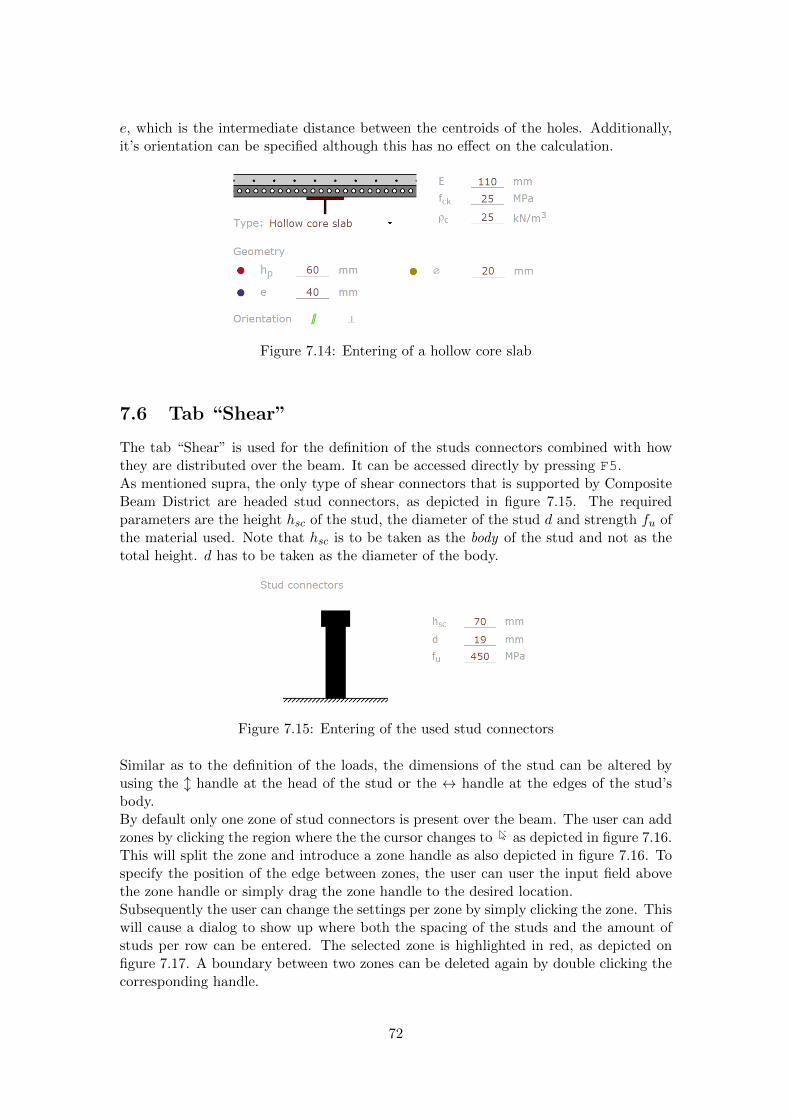
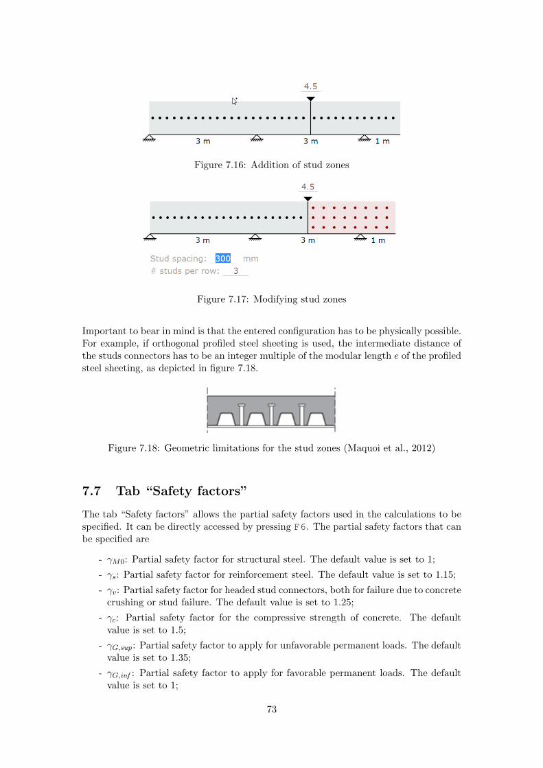
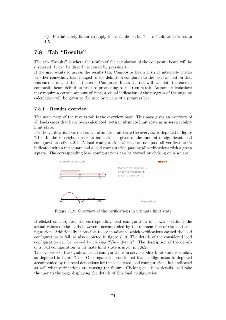
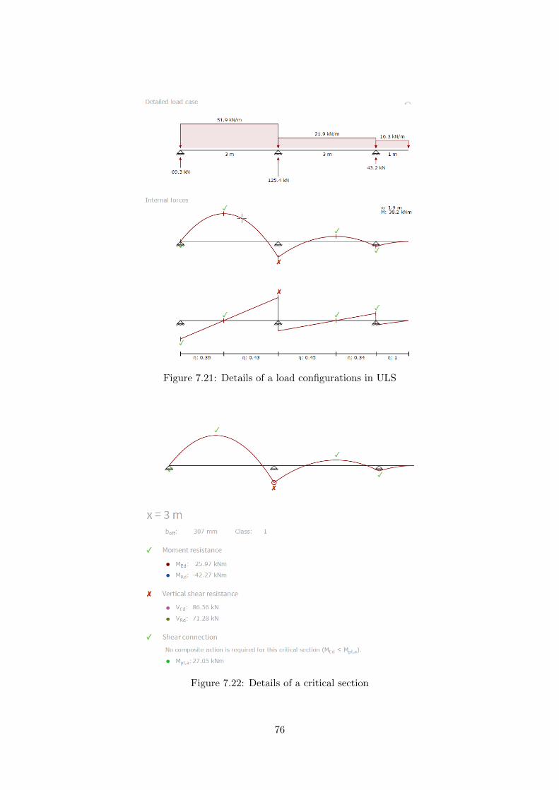
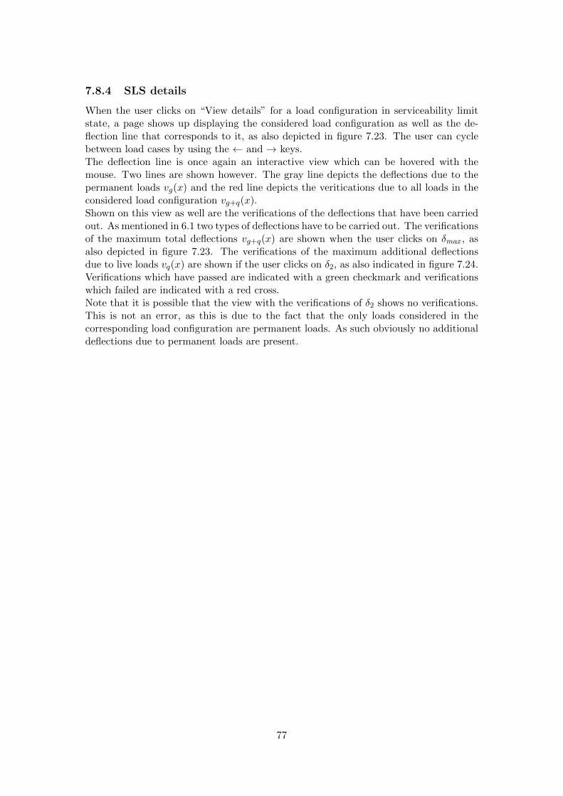
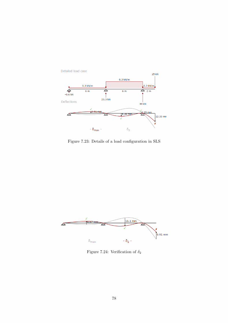
Sebastiaan Marynissen beams according to EC4 Development of a calculation software for composite Academic year 2014-2015 Faculty of Engineering and Architecture Chairman: Prof. dr. ir. Luc Taerwe Department of Structural Engineering Master of Science in Civil Engineering Master's dissertation submitted in order to obtain the academic degree of Counsellor: Dr. ir. Delphine Sonck Supervisor: Prof. ir. Rik Debruyckere
Transcript
Sebastiaan Marynissen
beams according to EC4Development of a calculation software for composite
Academic year 2014-2015Faculty of Engineering and ArchitectureChairman: Prof. dr. ir. Luc TaerweDepartment of Structural Engineering
Master of Science in Civil EngineeringMaster's dissertation submitted in order to obtain the academic degree of
Counsellor: Dr. ir. Delphine SonckSupervisor: Prof. ir. Rik Debruyckere
Preface
Ever since I was a little kid I was interested in everything that had to do with construc-tion, witness my creations in Duplo or at the beach in Wenduine. Through the yearsthis interest has become a true passion for structural analysis. At the age of 13 however,I became interested in computer programming as well, especially web development.The present master’s dissertation allowed me to merge my passion and my interest intosomething I could never have imagined before: Composite Beam District. The develop-ment of this software has proven to be so much more than simply programming formulasinto the computer. The present document has become a general document on how to de-velop constructional software and what obstacles and pitfalls can be encountered alongit’s way.The elaboration of this master’s dissertation never had been such an instructive expe-rience without a few people who I would like to thank. First of all I want to thank mysupervisor prof. ir. Rik Debruyckere for providing me the necessary information everytime I requested it and for the useful feedback, my counsellor dr. ir. Delphine Sonckand dr. ir. Iveta Georgieva for sharing thoughts on the development of software forcomposite beams.I would like to thank my family as well, especially my mother and father for giving meall the opportunities I have received, my nephew Jeroen for introducing me to websiteprogramming and my grandmother Josee.Another thank you goes to my friends of my student association Poutrix. You made mylast two years as a student a memorable period. A particular thank you goes to Laura.She knows why.At last I would like to thank Della Mae, to whose beautiful music I wrote a majorpart of this master’s dissertation. Music has always been an important part of my lifeand especially Della Mae’s music has guided me through the tough hours of huntingdown bugs which were buried deeply in the dungeons of the software’s source code. Irecommend them to anyone reading this master’s dissertation to experience the joyousfeeling their music induces.
Permission of use on loan
The author gives permission to make this master dissertation available for consultationand to copy parts of this master dissertation for personal use. In the case of any otheruse, the copyright terms have to be respected, in particular with regard to the obligationto state expressly the source when quoting results from this master dissertation.
Sebastiaan MarynissenMay 22, 2015
DisclaimerThe author, nor the supervisor, nor Ghent University can be held liable for direct orindirect damage as a result of any imperfections of the software and/or this document.
i
Overview
Master’s dissertation submitted in order to obtain the academic degree of Master ofScience in Civil Engineering
Title: Development of a calculation software for composite beams according to EC4
Author: Sebastiaan MarynissenSupervisor: Prof. ir. Rik DebruyckereCounsellor: Dr. ir. Delphine SonckResearch group: Laboratory for Research on Structural ModelsDirector: Prof. ir.-arch. Jan BelisDepartment: Department of Structural EngineeringChairman: Prof. dr. ir. Luc Taerwe
Faculty of Engineering and ArchitectureGhent UniversityAcademic year 2014-2015
Summary
In the context of the present master’s dissertation the software Composite Beam Dis-trict was developed. Composite Beam District is a software which calculates the internalforces and the deflections of a composite beam. The composite beam can be either sim-ply supported or continuous with in theory an unlimited amount of spans.
Based on the internal forces and the deflections Composite Beam District will performa a number of verifications which are in accordance with EN 1994-1-1:2004. The verifi-cations carried out in ultimate limit state are the resistance of the cross-section, whichincludes a verification of moment resistance and the resistance to vertical shear, a ver-ification for lateral torsional buckling and a verification of the shear connection. Inultimate limit state both the total deflection due to permanent and line loads as well asthe additional deflection due to live loads are verified.
The only load types that can be specified in Composite Beam District are uniformlydistributed surface loads on the concrete flange, uniformly distributed line loads actingdirectly on the steel profile and point loads.
4.1 Base cross-section . . . . . . . . . . . . . . . . . . . . . . . . . . . . . . . 324.2 Three-span continuous beam . . . . . . . . . . . . . . . . . . . . . . . . 334.3 Two-span continuous beam . . . . . . . . . . . . . . . . . . . . . . . . . 344.4 Effective width beff of a concrete flange, extracted from EN 1994-1-1:2004 354.5 Cantilever with a point load . . . . . . . . . . . . . . . . . . . . . . . . . 394.6 Moment lines for a point load of 1 kN . . . . . . . . . . . . . . . . . . . 394.7 Two-span continuous beam carrying a point load and a line load . . . . 404.8 Moment lines for all load configurations of figure 4.7 . . . . . . . . . . . 40
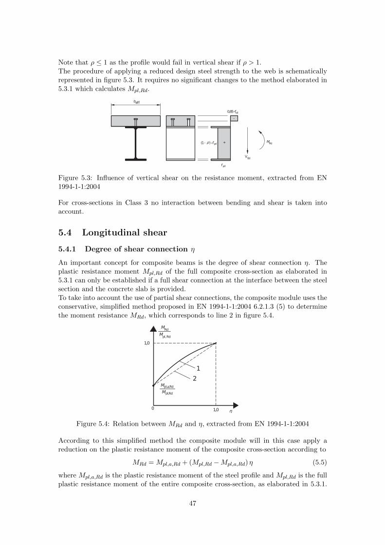
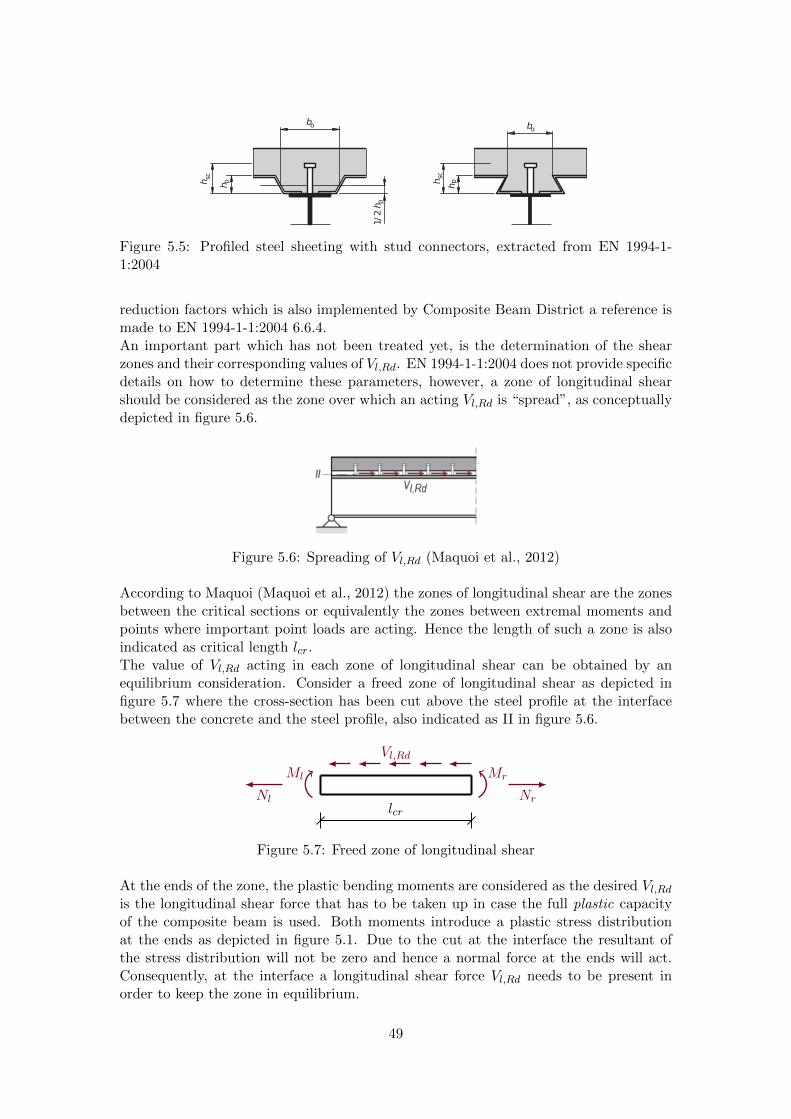
5.1 Example plastic stress distribution, extracted from EN 1994-1-1:2004 . 445.2 Reduction factor β, extracted from EN 1994-1-1:2004 . . . . . . . . . . 455.3 Influence of vertical shear on the resistance moment, extracted from EN
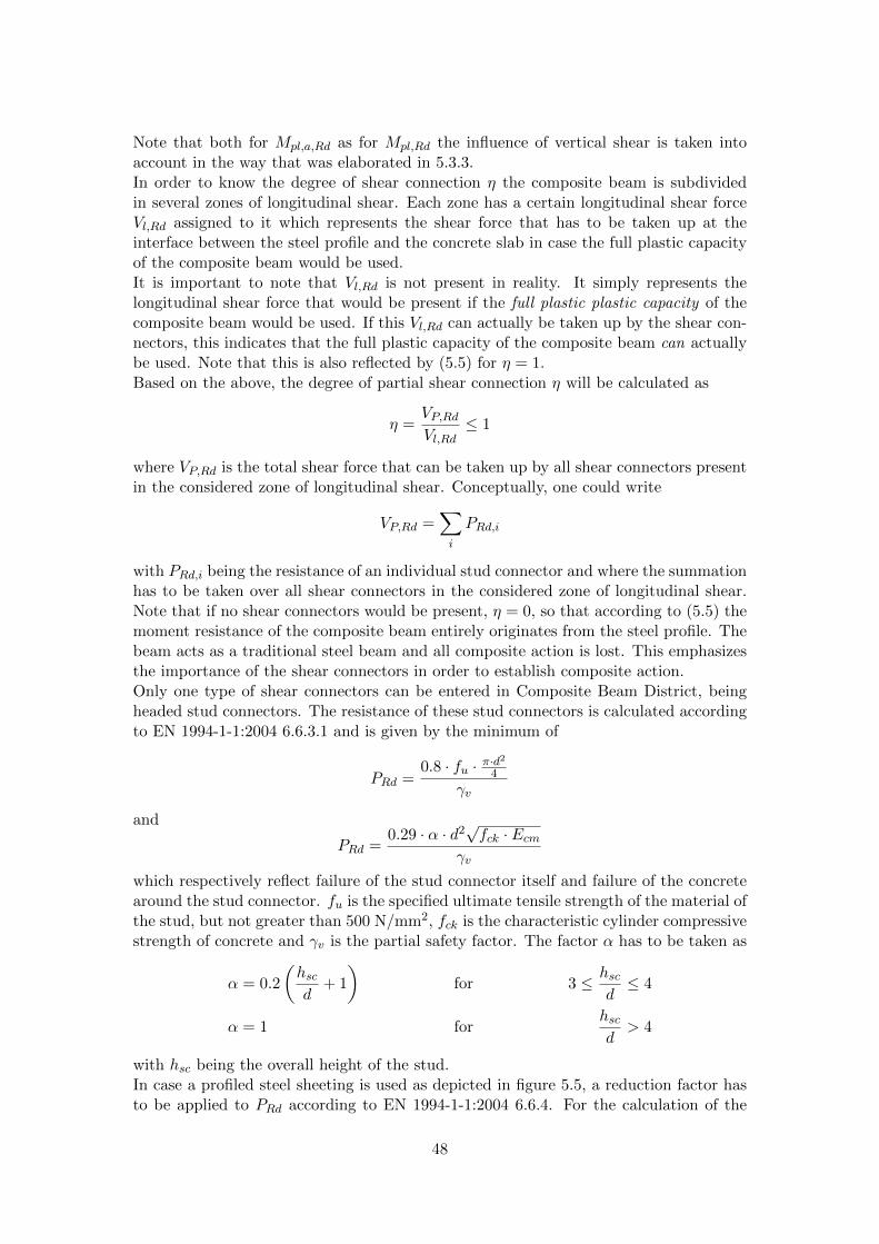
1994-1-1:2004 . . . . . . . . . . . . . . . . . . . . . . . . . . . . . . . . . 475.4 Relation between MRd and η, extracted from EN 1994-1-1:2004 . . . . 475.5 Profiled steel sheeting with stud connectors, extracted from EN 1994-1-
γv Partial safety factor for headed stud connector
ρ Factor representing the influence of vertical shear on bending
ρc Unit weight of concrete
xi
ϕi Left-end rotation of an element
ϕj Right-end rotation of an element
ξ Dimensionless coordinate of an element
Aa Total area of a steel profile
Af Area of the fictive steel section
Av Shear area
beff Effective width of a concrete flange
EIa Bending stiffness of the steel profile
fcd Design compressive strength of concrete
fck Characteristic cylinder compressive strength of concrete
fyd Design yield stress of structural steel
G Shear modulus of steel
hc Effective height of the concrete slab
Ic Moment of inertia of the fictive concrete section
If Moment of inertia of the fictive steel section
It Torsion constant of a steel profile
Iw Warping constant of a steel profile
Iz Moment of inertia around the weak axis of a steel profile
ks Rotational stiffness per unit length of steel beam to represent the invertedU-frame action
Le Distance between moment zeros
Mb,Rd Design lateral-torsional buckling resistance moment
Mcr Elastic critical moment for lateral-torsional buckling
Me(ξ) Moment line of an element
me(ξ) Dimensionless moment line of an element
Mpl,a,Rd Plastic resistance moment of the steel profile
PRd,i Shear resistance of an individual stud connector
Sf First moment of area of the fictive steel section
VRd Resistance to vertical shear
vd(x) Deflections due to the dead weight of the steel profile and the concrete slabonly
xii
ve(x) Deflection line of an element
vi Left-end vertical displacement of an element
vj Right-end vertical displacement of an element
vq(x) Additional deflections of a composite beam due to variable loads. Note thatvq(x) = vg+q(x)− vg(x)
vδp(x) Deflections due to the additional permanent loads
VEd Design value of the vertical shear force
vg+q(x) Deflections of a composite beam due to permanent and variable loads
vg(x) Deflections of a composite beam due to permanent loads only
VP,Rd Maximal longitudinal shear force that can be taken up by the stud connectorsin a considered zone of longitudinal shear
ws Unit weight of structural steel
xl Left offset of an element
xel Location of the elastic neutral axis
xpl Location of the plastic neutral axis
SLS Serviceability Limit State
ULS Ultimate Limit State
xiii
Any application that can be written in JavaScript, will eventuallybe written in JavaScript.
– Jeff Atwood
xiv
Chapter 1
Introduction
1.1 Scope
A composite beam consists out of three main parts:
- A steel profile;
- A concrete slab on top of the steel profile;
- A connection of both elements, mostly achieved by the use of headed stud connec-tors, which is crucial for a good co-operation.
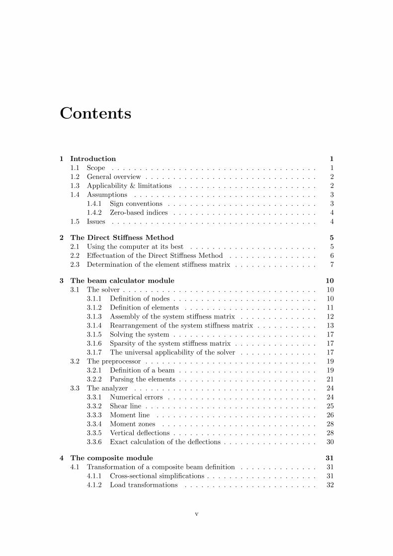
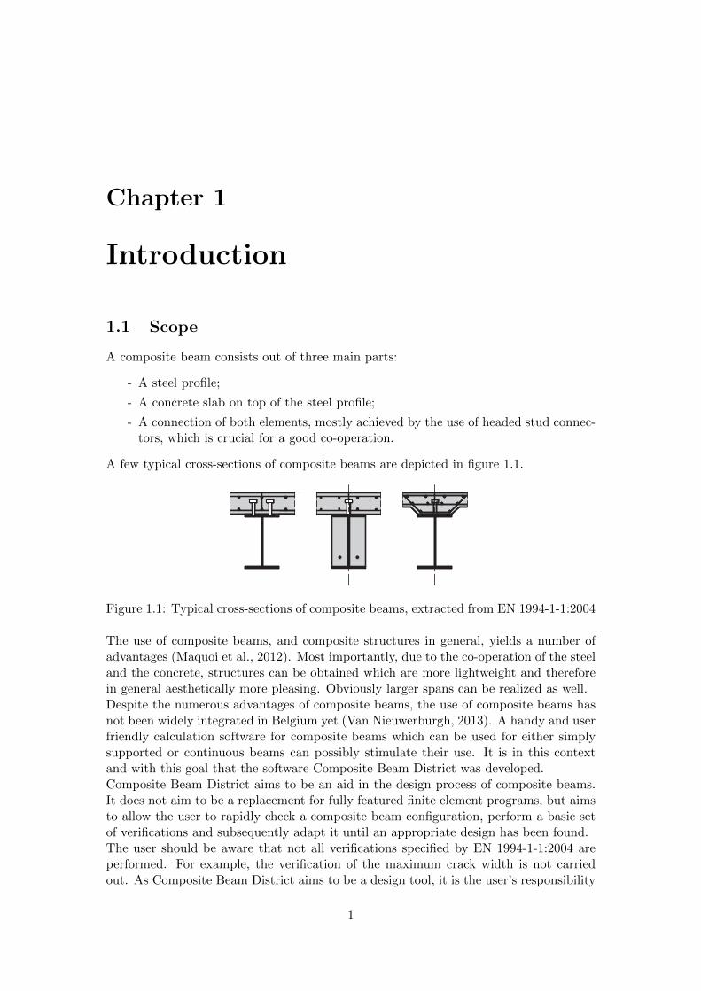
A few typical cross-sections of composite beams are depicted in figure 1.1.
Figure 1.1: Typical cross-sections of composite beams, extracted from EN 1994-1-1:2004
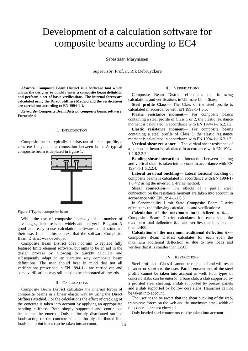
The use of composite beams, and composite structures in general, yields a number ofadvantages (Maquoi et al., 2012). Most importantly, due to the co-operation of the steeland the concrete, structures can be obtained which are more lightweight and thereforein general aesthetically more pleasing. Obviously larger spans can be realized as well.Despite the numerous advantages of composite beams, the use of composite beams hasnot been widely integrated in Belgium yet (Van Nieuwerburgh, 2013). A handy and userfriendly calculation software for composite beams which can be used for either simplysupported or continuous beams can possibly stimulate their use. It is in this contextand with this goal that the software Composite Beam District was developed.Composite Beam District aims to be an aid in the design process of composite beams.It does not aim to be a replacement for fully featured finite element programs, but aimsto allow the user to rapidly check a composite beam configuration, perform a basic setof verifications and subsequently adapt it until an appropriate design has been found.The user should be aware that not all verifications specified by EN 1994-1-1:2004 areperformed. For example, the verification of the maximum crack width is not carriedout. As Composite Beam District aims to be a design tool, it is the user’s responsibility
1
to perform the remaining verifications specified in EN 1994-1-1:2004 on his own once asuitable design has been found.
1.2 General overview
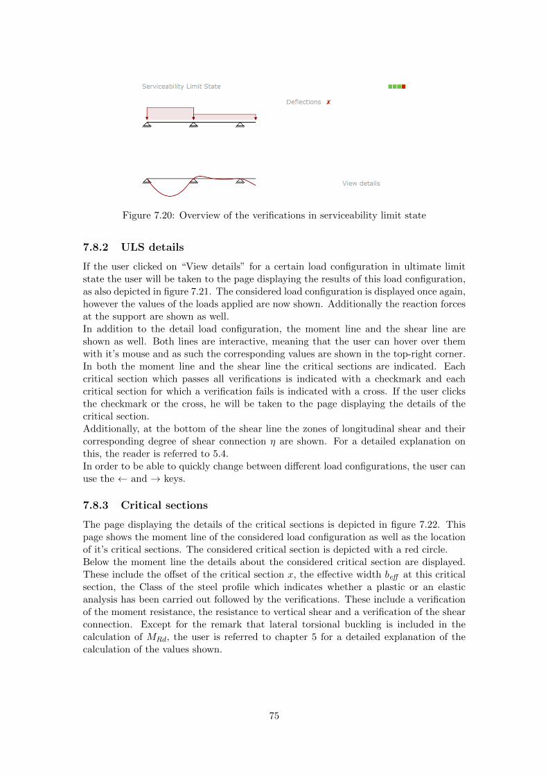
In general Composite Beam District consists out of two main parts: the graphical userinterface responsible for the input as well as the representation of the results and thecalculation module which calculates the configurations and performs a set of verifica-tions.The calculation module of Composite Beam District is in turn subdivided into two mainparts. The first part is the beam calculator module which is able to calculate the internalforces and deflections of an arbitrary beam configuration, regardless of it’s nature. Thebeam calculator module makes use of the direct stiffness method to calculate the beamconfigurations. As such this implies that the internal forces are calculated in a linearelastic way.The second part is the composite module. This module translates the composite beamconfiguration that was entered in the graphical user interface to a beam configurationwhich can be entered in the beam calculator module. Based on the results that it receivesfrom the beam calculator module it performs in ultimate limit state a verification of themoment resistance, hereby taking into account the effects of lateral torsional bucklingand the influence of the use of partial shear connections, a verification of the verticalshear resistance and a verification of the shear connections. In serviceability limit statethe composite module performs a verification of the maximum total deflection in eachspan as well as the maximum additional deflection due to live loads.The aim of this document is not to list up all the formulas of EN 1994-1-1:2004 whichhave been used for the verifications, but rather to provide some background informa-tion on the calculation methods, assumptions and design approaches implemented inComposite Beam District.
1.3 Applicability & limitations
Composite Beam District is applicable to composite beams for buildings as all imple-mented verifications are extracted from EN 1994-1-1:2004. It is possible to specify anarbitrary steel profile which is modeled as a set of steel plates. The steel profile cancontain multiple top-flanges and bottom-flanges. As such it is possible to represent asteel profile with welded additional flanges. Rolled steel profiles cannot be directly en-tered, but they can be approximated as a set of welded steel plates, hereby neglectingany roundings. In case a welded steel profile has to be entered, the fillet welds will beneglected as well. These approximations will result in a slightly conservative design, cfr.infra.In some composite beam configurations the steel profile is encased in concrete, as forexample depicted in figure 1.1. Such a configuration would increase the bearing capacitybut more importantly increase the fire resistance of the composite beam. Calculationsof the fire resistance are not implemented by Composite Beam District and as such noconcrete encasement can be entered. As for the bearing capacity, neglecting the concreteencasement will result in a conservative approach. Steel profiles of Class 4 cannot becalculated and will result in an error shown to the user.Four types of concrete slabs can be entered:
2
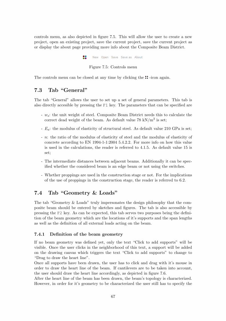
- A bare concrete slab;- A concrete slab supported by profiled steel sheeting;- A concrete slab supported by precast panels;- A concrete slab supported by hollow core slabs.
If a configuration has to be entered which does not use one of these types, the user isasked to enter an appropriate type which approximates best the type present in reality.The loads that can be entered are uniformly distributed surface loads acting on theconcrete slab, uniformly distributed line loads acting directly on the steel profile andpoint loads. All loads can be entered as either permanent or variable.As mentioned supra, Composite Beam District does not carry out all verifications speci-fied in EN 1994-1-1:2004. For example, shear buckling of the web and the verification oftransverse forces on the web is not implemented, nor is the verification of the maximumcrack width. The user has to be aware that these verifications will have to be carriedout manually.The influence of the construction stage is only taken into account for the calculation ofthe deflections. The construction stage can be verified by using existing software as inthe construction stage the beam can be considered as a steel beam carrying it’s owndead weight and the weight of the wet concrete.
1.4 Assumptions
1.4.1 Sign conventions
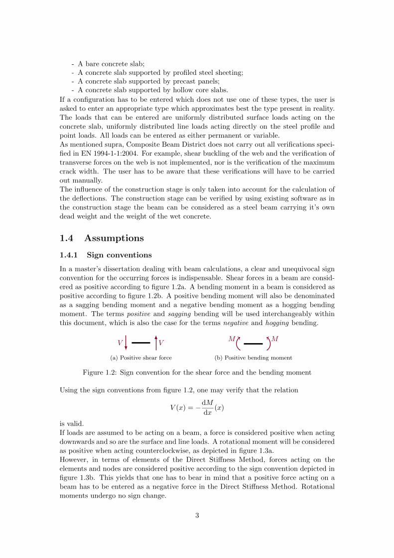
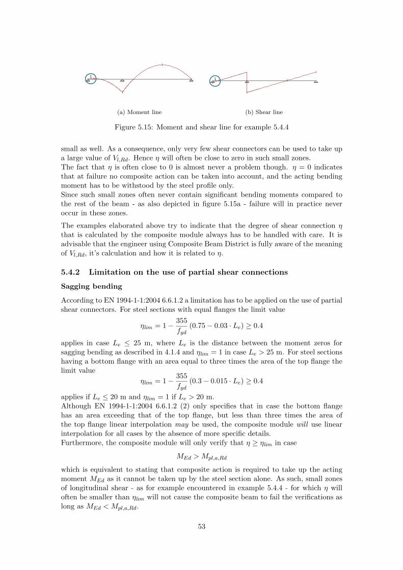
In a master’s dissertation dealing with beam calculations, a clear and unequivocal signconvention for the occurring forces is indispensable. Shear forces in a beam are consid-ered as positive according to figure 1.2a. A bending moment in a beam is considered aspositive according to figure 1.2b. A positive bending moment will also be denominatedas a sagging bending moment and a negative bending moment as a hogging bendingmoment. The terms positive and sagging bending will be used interchangeably withinthis document, which is also the case for the terms negative and hogging bending.
V V
(a) Positive shear force
M M
(b) Positive bending moment
Figure 1.2: Sign convention for the shear force and the bending moment
Using the sign conventions from figure 1.2, one may verify that the relation
V (x) = −dM
dx(x)
is valid.If loads are assumed to be acting on a beam, a force is considered positive when actingdownwards and so are the surface and line loads. A rotational moment will be consideredas positive when acting counterclockwise, as depicted in figure 1.3a.However, in terms of elements of the Direct Stiffness Method, forces acting on theelements and nodes are considered positive according to the sign convention depicted infigure 1.3b. This yields that one has to bear in mind that a positive force acting on abeam has to be entered as a negative force in the Direct Stiffness Method. Rotationalmoments undergo no sign change.
3
(a) Positive loads on a beam (b) Positive loads on an element
Figure 1.3: Sign convention for loads
1.4.2 Zero-based indices
An array is a commonly used data structure in most programming languages and as aconsequence they are used in Composite Beam District as well. Additionally, in mostprogramming languages the first element in an array has index 0. Therefore, whenreferred to offsets in arrays or vectors, the first element will be assigned offset 0, thesecond offset 1 and so on.
1.5 Issues
Although Composite Beam District is thoroughly tested by the use of unit testing1, it isimpossible to claim that it would be entirely free of bugs especially for the graphical userinterface as writing unit tests for a user interface is rather difficult and time consuming.If the user encounters a bug or an issue he is kindly requested to report it at https://github.com/sebamarynissen/composite-beam-district. At the date ofwriting (May 22, 2015), this repository is empty, but it is expected to have a wiki aswell as a download page for Composite Beam District anytime soon.
1Unit test are automated tests of the fundamental building blocks of a software. With every majorchange that is made it is good practice to run all unit tests. As such one can easily detect whetherchanges that were made have unexpected side effects. Unit tests should be written in such a way if alltests pass, one can be sure that everything works as expected.
4
Chapter 2
The Direct Stiffness Method
2.1 Using the computer at its best
As Composite Beam District aims to be suitable for an extensive range of configurations,it naturally should be able to handle statically indeterminate beams. This complicateshowever the determination of the internal forces of the beam, as the reaction forces -on which the internal forces depend - cannot be obtained directly from statics, and onewill need to take into account compatibility equations.A common way of tackling this problem is to use the principle of virtual work. As such,one expresses the displacements1 as a function of the statically indeterminate stressresultants and applies the compatibility conditions, which then supply the requiredequations to solve the system. Once the statically indeterminate stress resultants areknown, it is easy to calculate all the internal forces and deflections.While being very well suited for a hand calculation, the method is less suited for acomputer. This is because one has to choose which statically indeterminate stress re-sultants will be used. Therefore there is no clear procedure which can be implementedin a computer easily, because generalization is hardly possible.The Direct Stiffness Method circumvents the aforementioned problem. The Direct Stiff-ness Method is a powerful method and relatively easy to implement in a computer as itmodels the behavior of an entire set of bars into one single, linear matrix equation. Thesolving process of this matrix equation would be very cumbersome to elaborate by handdue to the large number of equations. For a computer this is however not an issue. Thecomputer is used for what it is good at: making calculations.As the Direct Stiffness Method subdivides the construction in a set of elements whichare interconnected, it can be considered as a kind of Finite Element Method. However,unlike regular FEM methods, the Direct Stiffness Method is exact within it’s assump-tions, meaning that after the discretization of the construction has been elaborated andsolved, the exact forces within an element can be found by using statics, whereas aregular FEM would only allow to approximate the exact forces, which is expressed bymeans of the interpolation functions.
1The word “displacement” is considered in the widest sense, representing both deflections and angularrotations.
5
2.2 Effectuation of the Direct Stiffness Method
For each element of the system, the forces2 acting on the edges of the element areexpressed as a function of the displacements. The obtained relationship for each elementcan be expressed as a matrix equation as
[Fe] = [Se] · [De] + [F 0e ] (2.1)
with [Fe] being the vector containing the forces acting on the edges, [Se] being theelement stiffness matrix, [De] being the vector containing all displacement components,and [F 0
e ] a vector containing force components originating from forces acting transverselyon the element. Thus, [Fe] and [De] can be written as
[Fe] =
YiMi
YjMj
[De] =
viϕivjϕj
where Yi and Yj represent the vertical forces at the respective edges i and j of theelement and Mi and Mj the rotational moments at the edges. Analogously, vi and vjrepresent the vertical deformations and ϕi and ϕj the angular rotations.In principle, (2.1) is expressed in coordinates which are bound to the element. In concreteterms this means that the displacements vi and vj are the displacements perpendicularto the center line of the undeformed element. In order to be usable, (2.1) has to beexpressed in system wide coordinates. When applying the Direct Stiffness Methodto for instance planar frames, this would require a matrix transformation. However,since Composite Beam District only deals with beams, which have an unambiguouslydefined center line, the element specific coordinates are the same for each element, andas such they can be directly used as system wide coordinates removing the need for atransformation to be applied.After the constitutive relationship (2.1) has been determined for each element, the equi-librium of each node is expressed by taking into account potential external forces actingon the node, as well as the contributions from the elements of which the considered nodeis part of. These contributions are expressed as a function of the displacements of theconsidered elements, contained in (2.1).For example, consider the node in figure 2.1 where elements 1 and 2 are joined and forwhich the rotational equilibrium is expressed. Me is an external moment acting on thenode.
•
Me
M1j M2i
1 2
Figure 2.1: Equilibrium of a node
Note that according to Newton’s third law, the moment exerted by the elements on thenode are equal in magnitude, but opposite in sign to the moments exerted by the nodes
2Like the general meaning of ”deformations”, ”forces” is considered to represent both actual forcesand rotational moments.
6
on the elements. Therefore, the rotational equilibrium of the node is expressed as
Me = M1j +M2i
Recall that M1j and M2i are functions of the displacements of their respective elementsaccording to (2.1).By expressing the equilibrium of all nodes, the entire system can be modeled with thesingle matrix equation
[S] · [D] = [L] (2.2)
with [S] being the system stiffness matrix, [D] being the vector containing all displace-ments and [L] being the vector representing the external influences on the system. Theprocess of constructing the system stiffness matrix by expressing the equilibrium of allnodes is called the assembly process. Due to the fact that (2.1) is a linear relationship,(2.2) is a linear set of equations.Once the system stiffness matrix has been determined, the boundary conditions areinserted into (2.2). For example, for a hinged support, the vertical displacement will be0, and as such a 0 will be filled in at the appropriate location in [D]. Note however thatthe vertical reaction of the hinged support is to be treated as an unknown external force.Therefore, at the offset where [D] has a known displacement component, an unknownexternal force will be present at the same offset in [L].The fact that both [D] and [L] contain unknown components does not change the natureof (2.2), as the sum of unknown displacement components and unknown reaction forcecomponents will also add up to the total amount of displacement components, and assuch sufficient equations will always be available. Therefore, the solving of (2.2) toall unknowns is only a matter of applying the known solution techniques from linearalgebra. As mentioned supra, this would be cumbersome to be elaborated by hand, butno problem at all for a computer.
2.3 Determination of the element stiffness matrix
One of the key parts of the Direct Stiffness Method which has not been treated into detailyet, is the determination of the element stiffness matrix. Consider the freed element infigure 2.2 with length l.
Mi Mj
Yi Yj
Figure 2.2: Free beam element
One may now express Yi and Yj as a function of Mi and Mj by expressing the rotationalequilibrium around respectively j and i from which
Yi =1
l(Mi +Mj)
Yj = −1
l(Mi +Mj)
(2.3)
is obtained.
7
Recall subsequently that the rotation θ of the ends of the element relative to it’s deflectedcenter line can be expressed as function of the absolute rotation of the end nodes ϕ andthe rotation of the beam element as
θi = φi −vj − vil
θj = φj −vj − vil
(2.4)
and as also depicted in figure 2.3.
vi
vjθi ϕi
θjϕj
Figure 2.3: Relative and absolute rotation of a node
Using the principle of virtual work one can express the moments Mi and Mj as a functionof the relative rotations θi and θj , as is also done in the slope deflection method, alsoknown as Gehler’s method (Van Impe, 2011). The expressions are
Mi =4EI
lθi +
2EI
lθj
Mj =2EI
lθi +
4EI
lθj
(2.5)
Substituting (2.4) in (2.5) delivers an expression of the moments Mi and Mj in functionof the displacements vi, vj , ϕi and ϕj . Additionally, substituting (2.5) in (2.3) resultsin an expression of the vertical forces Yi and Yj in function of the displacements vi, vj ,ϕi and ϕj .The expressions can be summarized in the element stiffness matrix as
[Se] = 2EI
l3·
6 3l −6 3l3l 2l2 −3l l2
−6 −3l 6 −3l3l l2 −3l 2l2
(2.6)
In order to take the influence of a uniformly distributed load on the element into account,the superposition principle is used. The forces Y 0
i , Y 0j , M0
i and M0j to keep the element
in equilibrium without a rotation or deflection of the ends are superposed to an unloadedelement. This situation corresponds to a clamped beam with a uniformly distributedload p acting on it, as depicted in figure 2.4.
p
Figure 2.4: Clamped beam with uniformly distributed load
8
Determining the reaction forces for this situation can be elaborated easily using virtualwork. One can verify that the reaction forces are given by
Yi =pl
2Yj =
pl
2Mi =
pl2
12Mj = −pl
2
12
or denoted as vector as
[F 0e ] =
pl
12
6l6−l
(2.7)
As such the consitutive relationship (2.1) has been elaborated.
9
Chapter 3
The beam calculator module
The beam calculator module that was implemented in the software uses an implemen-tation of the Direct Stiffness Method to calculate beam configurations in a linear elasticway. The Direct Stiffness Method in the software is implemented in three separate com-ponents: the solver, which is the very core, the preprocessor, which translates a beamconfiguration into a set of nodes and elements which can be used directly by the solver,and the postprocessor, also called the analyzer, which is able to generate moment andshear lines from the solved system.
3.1 The solver
The solver is implemented as general as possible, meaning it does not make any assump-tions about the nature of the problem. This way, it’s application is not limited to beamproblems. It will also result in a fundamental understanding of what a finite elementmethod is. For ease of understanding however, when explaining how the solver worksreferences to the application on beams will be made frequently.
3.1.1 Definition of nodes
A first essential component are the nodes. Nodes define the boundaries of the elementsand have a number of degrees of freedom assigned to it. In the context of the beams,each node has two degrees of freedom: a vertical displacement v and a rotation ϕ.The vertical displacement v is treated positive in the upward direction, and the nodalrotation ϕ is treated positive counterclockwise, as depicted in figure 3.1.
•v
ϕ
Figure 3.1: Degrees of freedom of a beam node
Additionally, at each node external influences1 may act. In the context of beams, theseinfluences are a potential vertical force F and a rotational moment M acting on thenode. These “forces” are treated positive in the same directions as the “displacements”v and ϕ.
1The word influence was intentionally used since the solver for the Direct Stiffness Method that wasimplemented does not know about the nature of the problem.
10
During the solving process some degrees are freedom are unknown, while others areknown, which is also the case for the influences acting on the node. To represent theunknown state, the special JavaScript type undefined is used. As such, a “bare” nodewith two degrees of freedom can be defined as depicted in listing 1.
var node = {freedom: [undefined,undefined
],influences: [undefined,undefined
]};
Listing 1: Definition of a node in JavaScript
“Bare” nodes cannot be used by the solver however, since such a bare node with twodegrees of freedom contains four unknowns, which will eventually result in a set ofequations with more unknowns than equations. Therefore, each node will have to becompleted as much as possible by the preprocessor. For example, in the context ofbeams, a simple support is modeled as depicted in listing 2.
var support = {freedom: [0,undefined
],influences: [undefined,0
]};
Listing 2: Definition of a support in JavaScript
For a simple support, the first degree of freedom, being the vertical displacement v,is fixed meaning v = 0. The rotation of the node however remains unknown, andis therefore still undefined. Conversely, the vertical reaction force of a support isinitially unknown, therefore it is entered as undefined, while the rotational momentis known.Note that in listing 2, the rotational moment is put equal to 0. This is not mandatory,since it is possible that a rotational moment is acting at a support. In this case, thevalue of the - known - rotational moment has to be entered.
3.1.2 Definition of elements
Along with the nodes, the elements are an essential component . Each element is boundby two nodes, but more importantly each element defines how these nodes influenceeach other.In the context of beams, this definition of how the two boundary nodes influence eachother is comprised in the constitutive relationship
[Fe] = [Se] · [De] + [F 0e ] (2.1)
11
where [Se] is the element stiffness matrix, representing the influence of a displacementon the forces to keep the element in equilibrium, and [F 0
e ] is the load vector taking intoaccount the contribution of a uniformly distributed load on the equilibrium forces.Consequently, each element e needs to be provided with three components by the prepro-cessor: an array containing the nodes the element contains, the stiffness matrix [Se] andthe load vector [F 0
e ]. As such, an element can be represented in JavaScript as depictedin listing 3.2
The data structures used to represent the matrices are simple arrays. In case of thestiffness matrix, this is a multidimensional array. The load vector however is a columnmatrix, which can be represented by a normal array.
At the start of the assembling process, the system stiffness matrix S is an m×m matrixfilled with zeros, with m being the number of degrees of freedom.To assemble the system stiffness matrix, the constitutive relationship of each elementhas to be expressed globally. Conceptually this is done by using location matrices.For example, consider a system with 3 nodes, each having 1 degree of freedom. Theconstitutive relationship between node 1 and node 2 can be written as(
f1f2
)︸ ︷︷ ︸[Fe]
=
(a bc d
)︸ ︷︷ ︸
[Se]
(d1d2
)︸ ︷︷ ︸[De]
+
(f01f02
)︸ ︷︷ ︸[F 0
e ]
(3.1)
Expressing this globally is done by multiplying the location matrix
Le =
1 00 10 0
with [Fe], [Se] and [F 0
e ] from (3.1), which results inf1f20
︸ ︷︷ ︸[Fe,g ]
=
a b 0c d 00 0 0
︸ ︷︷ ︸
[Se,g ]
d1d2d3
︸ ︷︷ ︸
[D]
+
f01f020
︸ ︷︷ ︸[F 0
e,g ]
2Due to the lack of an appropriate generalized naming for this “definition of influence”, the namesstiffness and loadVector are chosen, however the solver in principle does not know about thenature of the problem, as was mentioned before.
12
If [Fn] is the vector containing all external “influences” on the nodes, the equilibrium ofthe entire system can be expressed as∑
e
[Fe,g] = [Fn]
or equivalently ∑e
[Se,g]︸ ︷︷ ︸[S]
[D] = [Fn]−∑e
[F 0e,g]︸ ︷︷ ︸
[F 0]︸ ︷︷ ︸[L]
(3.2)
In practice, the multiplication with the location matrices doesn’t happen, as this wouldrequire a matrix multiplication three times for each location matrix, resulting in a largeoverhead, potentially causing performance issues. Instead the software assembles thesystem stiffness matrix [S] and the global force vector [F 0] as follows.For each element it is determined at which offset in the system stiffness matrix thesoftware should add the contributions from the element stiffness matrix of the currentelement. This offset is determined by a nodemap which was constructed in advance.This nodemap maps nodes to offsets in the global displacement vector [D]. As such, forboth nodes contained within the element the offsets in the global displacement vectorare determined. Combined with the number of degrees of freedom of the node, thecorrect offsets in the system stiffness matrix can be determined. The same happens forthe global load vector.
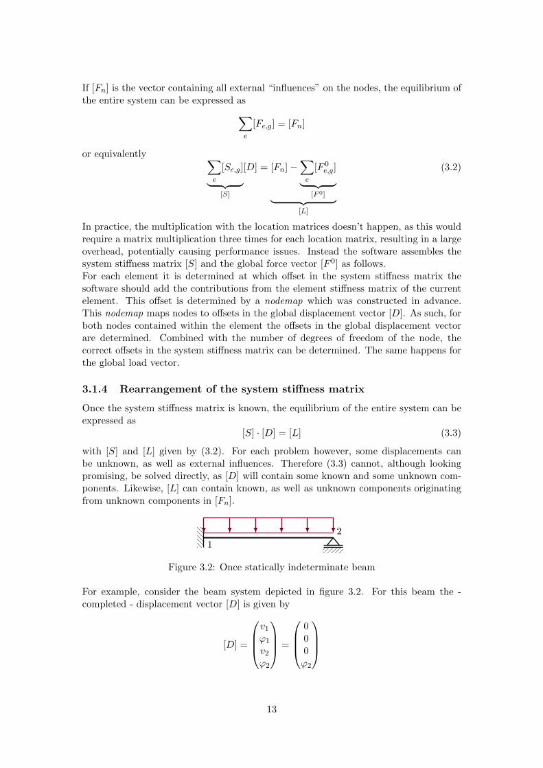
3.1.4 Rearrangement of the system stiffness matrix
Once the system stiffness matrix is known, the equilibrium of the entire system can beexpressed as
[S] · [D] = [L] (3.3)
with [S] and [L] given by (3.2). For each problem however, some displacements canbe unknown, as well as external influences. Therefore (3.3) cannot, although lookingpromising, be solved directly, as [D] will contain some known and some unknown com-ponents. Likewise, [L] can contain known, as well as unknown components originatingfrom unknown components in [Fn].
1
2
Figure 3.2: Once statically indeterminate beam
For example, consider the beam system depicted in figure 3.2. For this beam the -completed - displacement vector [D] is given by
[D] =
v1ϕ1
v2ϕ2
=
000ϕ2
13
as the only displacement which is unknown is the rotation ϕ2 at point 2. Likewise, [L]is found as
[L] =
R1 −pl
2
M1 −pl2
12
R2 −pl
2
pl2
12
as the reaction forces are still unknown.To tackle this problem, the unknown displacements and unknown reaction forces willseparated by rearranging the system asS1 S2
S3 S4
D1
D2
=
L1
L2
where [D1] is a submatrix only containing unknown displacements. As a consequence[L1] will only contain known components. As such all the unknown displacement com-ponents can be obtained by solving
[S1]︸︷︷︸A
· [D1]︸︷︷︸X
= [L1]− [S2] · [D2]︸ ︷︷ ︸B
(3.4)
to [D1]. After substituting [D1], [L2] is given by
[L2] = [S3] · [D1] + [S4] · [D2] (3.5)
Rearranging the vector with external nodal forces [Fn] as well as the global load vector[F 0] too, the unknown external forces to keep the system in equilibrium are found as
[Fn,2] = [S3] · [D1] + [S4] · [D2] + [F 02 ]
In the software, the rearrangement of the system is characterized by a swapmap. This isan array defining which offsets need to switch positions in another array. For example,consider the swapmap
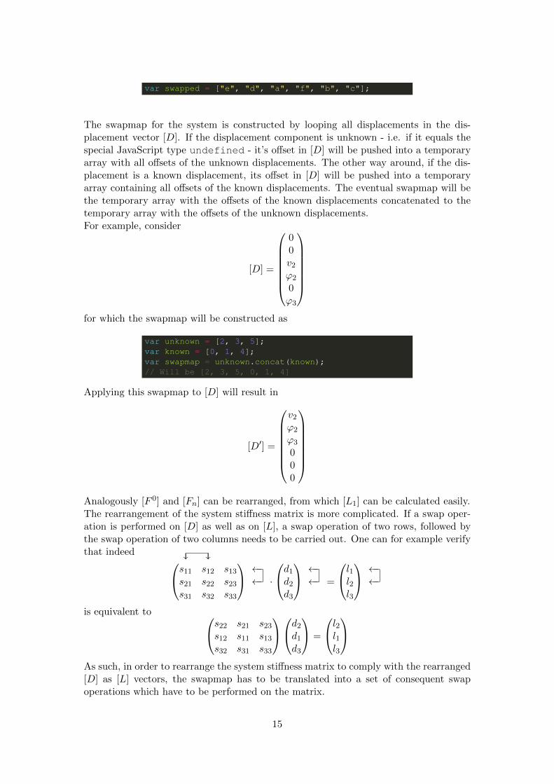
var swapmap = [4, 3, 0, 5, 1, 2];
Applied to another array, this swapmap will cause offset 4 in the target array to becomeoffset 0 in the result array. Offset 3 in the target array will become offset 1 in the resultarray etc. For example, consider the target array
var array = ["a", "b", "c", "d", "e", "f"];
Applying the swapmap on this array results in
14
var swapped = ["e", "d", "a", "f", "b", "c"];
The swapmap for the system is constructed by looping all displacements in the dis-placement vector [D]. If the displacement component is unknown - i.e. if it equals thespecial JavaScript type undefined - it’s offset in [D] will be pushed into a temporaryarray with all offsets of the unknown displacements. The other way around, if the dis-placement is a known displacement, its offset in [D] will be pushed into a temporaryarray containing all offsets of the known displacements. The eventual swapmap will bethe temporary array with the offsets of the known displacements concatenated to thetemporary array with the offsets of the unknown displacements.For example, consider
[D] =
00v2ϕ2
0ϕ3
for which the swapmap will be constructed as
var unknown = [2, 3, 5];var known = [0, 1, 4];var swapmap = unknown.concat(known);// Will be [2, 3, 5, 0, 1, 4]
Applying this swapmap to [D] will result in
[D′] =
v2ϕ2
ϕ3
000
Analogously [F 0] and [Fn] can be rearranged, from which [L1] can be calculated easily.The rearrangement of the system stiffness matrix is more complicated. If a swap oper-ation is performed on [D] as well as on [L], a swap operation of two rows, followed bythe swap operation of two columns needs to be carried out. One can for example verifythat indeed
y ys11 s12 s13s21 s22 s23s31 s32 s33
←−←− ·
d1d2d3
←−←− =
l1l2l3
←−←−
is equivalent to s22 s21 s23s12 s11 s13s32 s31 s33
d2d1d3
=
l2l1l3
As such, in order to rearrange the system stiffness matrix to comply with the rearranged[D] as [L] vectors, the swapmap has to be translated into a set of consequent swapoperations which have to be performed on the matrix.
15
For example, consider the list [a, b, c, d] and its rearranged form [b, d, c, a] to which theswapmap [1, 3, 0, 2] corresponds. The rearranged form can be obtained by three conse-quent swap operations:
Note that this can be obtained directly from the swapmap as
[↓1, 3, 0, 2] [1,
↓3, 0, 2] [1, 3, 0,
↓2]
or described in words: set the pointer in the swapmap at offset 0. The value at thisoffset is 1, indicating 0 ↔ 1. Next, shift the pointer to the value of the swapmap aswell, in this case offset 1. At offset 1 the value of the swapmap equals 3, so 1 ↔ 3 andshift the pointer to offset 3. At offset 3, the value of the swapmap equals 2, so 3 ↔ 2.At last, the pointer would be shifted to offset 2, where value 0 is encountered. On cansee that 0 ↔ 1 doesn’t have to be carried out though, which can be derived from thefact that offset 0 was already “affected” by the 0↔ 1 operation.Note that one needs to be aware of the fact that a swapmap may contain multipleindependent permutations. For example, consider the swapmap [2, 4, 3, 0, 1] with thecorresponding consequent swap operations
0↔ 2↔ 3 1↔ 4
which consequently contains two independent permutations.Taking all of the above into account, an algorithm rearranging the system stiffnessmatrix was developed, which is depicted in figure 3.3.
Data: swapmapData: system stiffness matrix [S]Result: rearranged system stiffness matrix [S′]set the pointer at 0;while still independent permutations do
get the value of the swapmap the pointer is pointing to;if this offset was already affected then
shift the pointer to an offset from the next independent permutation;else
swap the two rows and columns of the system stiffness matrix;shift the pointer to the value of the swapmap;
end
end
Figure 3.3: System stiffness matrix rearrangement algorithm
Note that [D] and [L] could have been rearranged with this algorithm as well, howeverthis causes an unnecessary overhead, as the swapmap explicitly defines the final stage ofthe vector to be rearranged, eliminating the need of knowing the series of swap operationsthe swapmap corresponds with.
16
3.1.5 Solving the system
Once the system stiffness matrix [S] as well as [D], [F 0] and [Fn] are rearranged, theunknown degrees of freedom are solved easily using (3.4). The solver does not do thisitself, but relies on an external library called numeric.js (Loisel, 2012) which is able tosolve a linear set of equations of the form
A ·X = B
After the unknown force components are also obtained according to (3.5), the solvercompletes all nodes with the degrees of freedom that it has calculated, as well as theunknown force components, which represent the calculated reaction forces.
3.1.6 Sparsity of the system stiffness matrix
Characteristic to finite element problems is that the system stiffness matrix [S] willcontain a lot of zeros due to the fact that only a limited number of elements are inter-connected, which is the case as well for beams solved using the Direct Stiffness Method.The relative amount of nonzero elements in a matrix is also known as the sparsity of amatrix.One may opt to store only the nonzero entries of the matrix instead of the entire matrixas this will result in a severe reduction of memory usage. The data structure usedto represent such sparse matrices can for instance be the Yale sparse matrix format(Eisenstat et al., 1983).The problem with this approach however is that the solving process can become quitecomplicated. Therefore, due to the limited nature of beam problems, the full matricesare used by the solver. Tests with the implementation of the solver have shown thateven for continuous beams with 100 spans - which is far from realistic - no significantmemory issues arise.
3.1.7 The universal applicability of the solver
As mentioned before, the solver was implemented in such a way that it does not knowabout the nature of the problem. Every linear problem consisting out of a set of nodesand elements, which can be modeled as
[S] · [D] = [L]
can therefore be solved. A few examples will be elaborated to illustrate this.
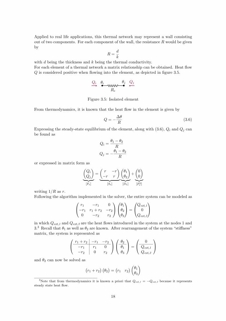
Example 3.1.1. Consider the steady-state thermal network depicted in figure 3.4 withthree nodes, each having a certain temperature θ. Between the nodes resistant elementsare present, each characterized by their resistance R. Assume that θ1 and θ3 are knownand the goal is to find θ2.
•θ1
R1
•θ2
R2
•θ3
Figure 3.4: Simple thermal network
17
Applied to real life applications, this thermal network may represent a wall consistingout of two components. For each component of the wall, the resistance R would be givenby
R =d
k
with d being the thickness and k being the thermal conductivity.For each element of a thermal network a matrix relationship can be obtained. Heat flowQ is considered positive when flowing into the element, as depicted in figure 3.5.
•θi
Re•θjQi Qj
Figure 3.5: Isolated element
From thermodynamics, it is known that the heat flow in the element is given by
Q = −∆θ
R(3.6)
Expressing the steady-state equilibrium of the element, along with (3.6), Qi and Qj canbe found as
Qi =θ1 − θ2R
Qj = −θ1 − θ2R
or expressed in matrix form as(QiQj
)︸ ︷︷ ︸[Fe]
=
(r −r−r r
)︸ ︷︷ ︸
[Se]
(θ1θ2
)︸ ︷︷ ︸[De]
+
(00
)︸︷︷︸[F 0
e ]
writing 1/R as r.Following the algorithm implemented in the solver, the entire system can be modeled as r1 −r1 0
−r1 r1 + r2 −r20 −r2 r2
θ1θ2θ3
=
Qext,1
0Qext,3
in which Qext,1 and Qext,3 are the heat flows introduced in the system at the nodes 1 and3.3 Recall that θ1 as well as θ2 are known. After rearrangement of the system “stiffness”matrix, the system is represented as r1 + r2 −r1 −r2
−r1 r1 0−r2 0 r2
θ2θ1θ3
=
0
Qext,1
Qext,3
and θ2 can now be solved as(
r1 + r2) (θ2)
=(r1 r2
)(θ1θ3
)3Note that from thermodynamics it is known a priori that Qext,1 = −Qext,3 because it represents
steady state heat flow.
18
or
θ2 =r1θ1 + r2θ3r1 + r2
One may recall from thermodynamics that this is indeed correct.
Example 3.1.2. Consider the three spring system depicted in figure 3.6. Each springhas a spring constant k, and two forces act with a magnitude of 1, but with oppositedirections in nodes 2 and 3, as also depicted in figure 3.6.
k1•
k2•
k3
1 1
Figure 3.6: Three spring system
For each spring one can verify that expressing the force equilibrium of the spring leadsto (
FiFj
)︸ ︷︷ ︸[Fe]
=
(k −k−k k
)︸ ︷︷ ︸
[Se]
(uiuj
)︸ ︷︷ ︸[De]
+
(00
)︸︷︷︸[F 0
e ]
assuming displacements and forces as positive from left to right. As such, the solver willassemble the system stiffness matrix so that the system can be expressed as
k1 −k1 0 0−k1 k1 + k2 −k2 0
0 −k2 k2 + k3 −k30 0 −k3 k3
0u2u30
=
F1
1−1F4
with F1 and F4 being the unknown reaction components. After rearrangement of thesystem this yields
k1 + k2 −k2 −k1 0−k2 k2 + k3 0 −k3−k1 0 k1 0
0 −k3 0 k3
u2u300
=
1−1
F1
F4
Analogously to the thermal network, u2 and u3 can be easily obtained by solving(
k1 + k2 −k2−k2 k2 + k3
)(u2u3
)=
(1−1
)after which F1 and F4 are obtained directly by substitution of u2 and u3.If all springs have a stiffness of 1, u2 = 1/3 and u3 = −1/3. The forces at the clampsare respectively −1/3 and 1/3.
3.2 The preprocessor
3.2.1 Definition of a beam
As mentioned above, the solver simply solves a system consisting out of several elements,regardless of what the nature of the system is. Therefore, it is required to pass the solver
19
a set of nodes and elements, with the behavior already defined. As such it would berequired to input elements and nodes, as defined in listing 3 and 1, manually. Since thisis not practical, the processor is delegated the responsibility to convert a definition of abeam into a set of elements which can be entered into the solver.A definition of a beam that has to be calculated consists out of three parts. The moststraightforward is of course the geometry of the beam. The geometry is characterized bythe subsequent span lengths, but also by the support conditions. For example, a simplysupported beam with a length of 2 m is entered in JavaScript as
var geometry = ["o", 2, "o"];
where o represents a simple support. A one-sided clamped beam with a length of 1 mis entered as
var geometry = ["|", 1];
with | representing the clamped support. As a final example, a simply supported beamwith a left cantilever of 1 m and a central span of 2 m is entered as
var geometry = [1, "o", 2, "o"];
The second important part is the definition of the loads. Two types of loads are allowed:point loads and uniformly distributed line loads. A point load is characterized by it’svalue in kN and it’s absolute offset in m, where x = 0 corresponds with the left end ofthe beam. As such, a point load is entered as
var load = {"offset": 1,"value": 10
};
Analogously a line load requires an interval to be specified and a value in kN/m and isentered as
var load = {"interval": [1, 3],"value": 5
};
Finally, a distribution of the bending stiffness is required. Note that this only plays arole in case of statically indeterminate beams, and more specifically only the relativeratio of the bending stiffnesses plays a role. Therefore, the units in which the bendingstiffnesses are entered are irrelevant, as long as they are expressed in the same units.As a consequence, for statically determinate beams, one may as well enter the value of1 for the entire beam. As such, the distribution of the bending stiffness over the beamis entered in JavaScript as
20
var stiffness = {"interval": [0, 4],"value": 1
};
and the complete distribution is entered as an array of these objects. Note that carehas to be taken that the specified intervals cover the entire length of the beam.
Example 3.2.1. Consider the two-span beam with a cantilever at it’s right end asdepicted in figure 3.7 carrying a line load of 4 kN/m and two point loads of 1 kN atrespectively 2 m and 7 m. The beam has a constant bending stiffness EI of 1.
4 m 3 m 1 m
1 kN 1 kN
4 kN/m
Figure 3.7: Two-span beam with a cantilever
This beam configuration will be entered in the beam calculator module as depicted inlisting 4.
Listing 4: JavaScript representation of the beam depicted in figure 3.7
3.2.2 Parsing the elements
In order determine the internal forces and hence solve the beam configuration, a beamdefinition such as the one depicted in figure 3.7 and represented in listing 4 has to beconverted into a system which can be entered directly into the solver. More specifically,
21
a set of nodes and elements has to be constructed as depicted in respectively listing 1and 3 based on the beam definition.The preprocessor does this by an algorithm which makes use of the concept of a “point ofinterest”. Such a point of interest contains the offset x of the point, a property called δpwhich represents the jump in line load encountered at the point of interest, a propertycalled δEI representing the jump in bending stiffness EI encountered at the point, aproperty called b, which is an array containing two numbers which can be either 0 or 1which represent the degrees of freedom of point of interest and a property called e whichis an array containing the external loads acting on the point of interest. The externalloads are respectively a potential point load and a potential rotational moment. Afterall points of interest have been found they will all be converted into actual nodes whereany coinciding points of interest are merged into the same node.First of all, the preprocessor determines all points of interest originating from the def-inition of the geometry. For the beam definition considered in example 3.2.1, the pre-processor will find points of interest at offsets 0, 4, 7 and 8. The points at offsets 0, 4and 7 are all simple supports meaning that the property b will be set to [1, 0] where 1indicates that the considered degree of freedom is fixed. Indeed, for a simple support thevertical displacement is fixed. Likewise 0 indicates that the considered degree of freedomis unrestrained, which is the case for the rotation at a simple support. Similarly thepreprocessor will set the property b of the point of interest at offset 8 to [0, 0] as thisis a free end of the beam and hence a free node. Note that for all points of interestencountered by considering the beam geometry δp, δEI and e will be set to 0.Subsequently the preprocessor will determine all points of interest originating from thedefinition of the point loads. This is fairly simple as at each point load a point of interestwill be introduced, where e is set to [F, 0] where F is the value of the point load actingin this point4. Both δp and δEI are set to 0 and b is set to [0, 0].After the points of interest for the point loads have been determined, the preprocessorwill determine the points of interest for the line loads. At the starting point of each lineload, a point of interest is introduced with δp = p where p is the value of the line load.At the end of the line load another point of interest is introduced with δp = −p. e willbe set to [0, 0] and b will be set to [0, 0], even if the point of interest would coincide witha support. δEI is set to 0.The points of interest for the bending stiffness distribution are determined in the sameway as for the line loads. At each starting point of a bending stiffness interval, a pointof interest is introduced with δEI = EI where EI of course represents the value of thebending stiffness in that interval. At the end of the interval another point of interest isintroduced with δEI = −EI . Again, e is set to [0, 0], b is set to [0, 0] and δp = 0.Additionally, the beam calculator module allows offsets to be specified at which a nodewill be introduced regardless of whether a point of interest will be detected at this offset.All offsets can be specified as an array. At each offset a point of interest is introducedwith δp = δEI = 0, e = b = [0, 0].Once all points of interest have been determined, the preprocessor will first merge allpoints of interest which have the same offset x. During this merge process, δp is found
4One may wonder why the e property of a point of interest provides the possibility to specify anexternal rotational moment where this is never used in the context of Composite Beam District. Thisis implemented for the sake of completeness. As such the beam calculator module can be used indepen-dently as well outside of the context of composite beams.
22
asδp =
∑i
δp,i
where the summation has to be effectuated over all points of interest i with the sameoffset x. Similarly δEI is found as
δEI =∑i
δEI ,i
The e property is constructed in a similar way as
e =
[∑i
ei[0],∑i
ei[1]
]
The b property of the merged point of interest is constructed as
b =
[1−
∏i
(1− bi[0]) , 1−∏i
(1− bi[1])
]
Consider for example three points of interest that coincide where one point of interestyields b = [1, 0] and the other two yield b = [0, 0], which for instance will be the case ifa support coincides with the start of a line load and a bending stiffness interval. In thiscase, the merged point of interest will yield
b = [1− 0× 1× 1, 1− 1× 1× 1 ] = [1, 0]
which is indeed the required behavior.After all points of interest have been merged, then will be sorted by their offset and foreach point of interest a node according to listing 1 is introduced where the freedomproperty is obtained from b and the influences property is obtained from e.Subsequently all elements are constructed as well by looping all sorted points of interestwhere the uniformly distributed load pi of each element i is obtained as
pi =∑j<i
δp,j
and the bending stiffness EI as
EI i =∑j<i
δEI ,j
The length li of each element i is of course found as
li = xi+1 − xi
where xi represents the offset of the point of interest i.One can now construct all elements as depicted in listing 3 where the two nodes areof course the nodes that were constructed from the points of interest i and i + 1. Theelement stiffness matrix [Se] is determined according to (2.6) and the load vector [Fe]according to (2.7). Together all nodes and elements form the “bare” system representingthe beam defintion. This “bare” system can be entered directly into the solver.
23
3.3 The analyzer
The analyzer is responsible for the interpretation of the results which were obtainedby the solver. As mentioned supra, the solver does not know about the nature of theproblem, whereas the analyzer does know about the nature. So to speak, the analyzertranslates the results obtained by the solver, which in the context of beams representthe deformations v and ϕ of each node, into properties which are relevant in terms ofstructural analysis, such as the moment line.As input the analyzer receives the displacement vector [D] of the entire system which atthis point contains no more unknowns as it has been solved by the solver as explainedsupra. From [D] it extracts the displacement vector [De] of each element after which iteffectuates the matrix multiplication
[Fe] = [Se] · [De] + [F 0e ] (2.1)
from which Yi, Yj , Mi and Mj as depicted in figure 2.2 are found. Combined withthe uniformly distributed load p acting on the element this provides all the requiredinformation to determine the internal forces as well as the deflections.
3.3.1 Numerical errors
Inevitable due to the discrete nature of how a computer effectuates calculations withfloating point numbers is that numerical errors will be present. For example, considerthe expression
var a = 0.1 + 0.2;
in JavaScript (Croxall, 2011). In contrast to what one may think, the value of thevariable a will not be 0.3 but 0.30000000000000004. The reason is that the computerimmediately converts 0.1 to it’s binary representation. As 2 is the base number of thebinary number system, 0.1 has to be written as
0.1 = ai
∞∑−∞
2i
where ai is either 0 or 1. The problem is that the machine precision is too low torepresent 0.1 in the binary number system. For example, when using a precision of 12digits, 0.1 can only be approximated as
0.1 ≈ 1
24+
1
25+
1
28+
1
29+
1
212
= 0.09985351562
or binary written as 0.000110011001. Likewise 0.2 can only be approximated in binarywith a precision of 12 digits as
0.2 ≈ 1
23+
1
24+
1
27+
1
28+
1
211+
1
212
= 0.19995117187
or written in binary as 0.001100110011.
24
Initially one may be in the belief that these type of numerical errors do not introducespecific difficulties. Surely whether the acting bending moment on and end support isactually 0 or 1× 10⁻¹⁶ will not be crucial for the verifications carried out on the beam.However numerical errors definitely have to be feared when for instance the zeros ofthe moment line - which are often relied on, cfr. infra - have to be determined. Forexample, consider two adjacent elements e1 and e2 which are part of a certain beamsystem. In principle, if no external moment is acting on the shared node between e1and e2, according to the rotational equilibrium of the shared node
M2i +M1
j = 0 (3.7)
where M1j is the moment acting on element e1 at its right edge and M2
i is the momentacting on element e2 at its left edge, as also depicted in figure 3.8.
•M1j
M2i
Figure 3.8: Moments acting on the edges of elements e1 and e2
However, due to the numerical errors introduced by the effectuation of (2.1), the equi-librium (3.7) will generally not be fulfilled. This specifically is an issue when M1
j and
M2i have the same sign, which would imply a discontinuity in the bending moment line
where more importantly the sign of the bending moment changes as well. As a conse-quence, if the zeros of the bending moment line have to be determined, no zeros will bedetected in the neighborhood of the shared node and hence the moment zones will bedetermined incorrectly.To tackle this problem, the analyzer will force the moment line to be continuous. Thisis done by looping all beam elements starting from the second beam element. For eachelement with index k, the analyzer will calculate the “shift distance” δM as
δM = Mk−1j +Mk
i
Subsequently the analyzer will put
Mk−1i = −Mk−1
j
andMkj = Mk
j + δM
which corresponds to shifting the moment line of element k up with a distance of δM .Note that it is important that Mk
i is explicitly put equal to −Mk−1j as effectuating
Mki = Mk
i + δM would introduce new numerical errors, causing Mk−1j 6= −Mk
i implyingthe moment line to remain discontinuous.
3.3.2 Shear line
The shear line of the entire beam is found as the concatenation of the shear lines of allelements in the beam system. As for each element the vertical force acting on the leftedge of the element Yi as well as the uniformly distributed load p are known, the shearline for each element is obtained as
Ve (ξ) = −Yi + pl · ξ (3.8)
25
where ξ is the dimensionless coordinate x/l with l being the length of the element. Thedimensionless coordinate ξ of an element is used very often by the analyzer as it willgreatly enhance the elegance of the used formulas, cfr. infra.Note that as the value of the shear line has to be obtained from the shear line of theappropriate element, a decent way has to be implemented to grab that element. A naiveapproach would be that in case the value of the shear force at offset x is requested allelements of the beam will be looped and for each element it is checked whether the offsetx is contained within this element. This however requires all elements of the beam tobe looped every single time the value of the shear force at an offset x is requested.The analyzer tackles this problem by constructing an interval tree of all elements in thebeam. In computer science, an interval tree is a tree data structure to hold intervals(de Berg et al., 1997). It allows for fast queries to obtain all intervals that either containa specific point or are overlapping with a given interval due to the fact that it keepstrack of the order of all intervals. A library with a decent implementation of intervaltrees in JavaScript was found in the interval-tree library (Suzuki et al., 2011). 5
As such, the analyzer constructs an interval tree containing all elements. If the valueof the shear force at a certain offset x is requested, the constructed interval tree will bequeried for the element containing this offset, which happens in a binary way which willgreatly reduce the query time. Once the element containing offset x is found, ξ is givenby
ξ =x− xll
where xl is the left offset of the element and l is the length of the element. This value ofξ is subsequently entered into the shear line function Ve(ξ) of the element as expressedin (3.8) after which the desired value of V (x) is obtained.
3.3.3 Moment line
Analogous to the shear line of the beam system, the moment line is found as the con-catenation of the moment lines of each element. For each element, both Mi and Mj
have been calculated by the analyzer and combined with the uniformly distributed loadp that acts on the element the moment line of the element will be parabolic. The generalshape of an element’s moment line is hence depicted in figure 3.9.
Mi Mj
Figure 3.9: Moment line for an element
Once again the dimensionless coordinate ξ will be used. One may subsequently verifythat the moment line Me (ξ) for an element is given by
Me(ξ) = 4 · pl2
8(1− ξ) ξ + (Mj +Mi) · ξ −Mi (3.9)
5The interval-tree library initially was not capable however of treating intervals with floating pointsnumbers as boundaries. This was resolved by manually fixing the issue and requesting the creator ofthe interval-tree library to apply this fix as well. As such, the author has been added to the list ofcontributors to the library.
26
Recall that p is considered as positive when acting downwards and that the bendingmoment in an element is considered positive in accordance with the sign conventiondepicted in figure 1.2b. Hence, Me(0) = −Mi and Me(1) = Mj .The procedure to obtain the value of the bending moment at a given offset x is completelyanalogous to the procedure for the shear line using the interval tree that was constructedto determine the appropriate element.Unlike the shear line which cannot reach an extreme value within an element due to it’slinearity which is a consequence of the fact that p is uniformly distributed which is alsoreflected by
p =dV
dxthe moment line can reach an extremal value within an element. Persisting to thedimensionless philosophy, one may refactor (3.9) to
me(ξ) =ξ
2(1− ξ) + (mj +mi) · ξ −mi (3.10)
by writing Me(ξ) = pl2 ·me(ξ) where me(ξ) hence is the dimensionless moment line ofthe element. Using expression (3.10) the location of the extreme bending moment canbe obtained by expressing
dme
dξ(ξ) = 0
which yields
ξ0 = mj +mi +1
2(3.11)
Note that if ξ0 < 0 or ξ0 > 1, the moment line does not reach an extreme withinthe element. If 0 ≤ ξ0 ≤ 1, the extreme value of the bending moment is found bysubstituting (3.11) in (3.9).Along with the location and the value of any extremal bending moment, the location ofthe zeros of the bending moment line are of importance as well, in particular in orderto determine the moment zones, cfr. infra. If any zeros of the moment line occur withinan element, their dimensionless offset can be found by expressing
me(ξ) = 0
and solving the corresponding quadratic equation. In expanded form, this equation canbe written as
ξ2
2−(
1
2+mj +mi
)ξ +mi = 0
for which the solution is found as
ξ0 =1
2+mj +mi ±
√(1
2+mj +mi
)2
− 2 ·mi
Important to note is that if p = 0 for the considered element, the moment line would belinear and be given by
M(ξ) = (Mj +Mi) · ξ −Mi
and ξ0 is obtained as
ξ0 =Mi
Mj +Mi
Again, if ξ0 < 0 or ξ0 > 1, the analyzer will omit this zero for the considered element asit is not contained within the considered element.
27
3.3.4 Moment zones
Of importance as well is to be able to determine the so called “moment zones”. Undermoment zones the sign of the bending moment over the entire beam is understood. Thisis especially important for structures where concrete is used as a material - which is ofcourse a key point in composite beams - as concrete will generally not be taken intoaccount when acting in tension.The analyzer determines the moment zones as intervals with each a sign assigned toit. Initially, the bending moment of the left-most element is requested. The sign of thefirst moment zone will be the sign of this bending moment. However, if the bendingmoment at the left end would be 0, the sign of the first moment zone is determined byconsidering
V = −dM
dx
Hence, if the shear force V at the left end of the left-most element is negative, the firstmoment zone will have a positive sign and a negative sign if V is positive. Recall thatV is taken as positive in accordance with 1.2a, which means that V (0) = −Yi, which isalso in accordance with (3.8).If V would be 0 as well, the analyzer resorts to the uniformly distributed load p of theelement, as according to
p = −d2M
dx2
with p positive when acting downwards. Hence, if p < 0, the first moment zone willbe negative taken into account that M(0) = V (0) = 0. Conversely, if p > 0, the firstmoment zone will be assigned a positive sign.Once the analyzer has determined the sign of the first moment zone, all elements ofthe beam will be looped. For each element it is requested whether any moment zerosare contained within the element in accordance with 3.3.3. Consequently the momentzone that was already “opened” is “closed” and the sign of the new moment zone tobe created is determined using the same procedure as described above by using thederivatives. The reason why this is done instead of simply counting on a sign changeis that theoretically it is possible that the moment line reaches a zero where the shearforce - or equivalently the derivative of the moment line - is zero as well. In this case,no sign change will occur as the moment line will always be parabolic.Once all elements of the beam have been looped, the last “open” moment zone is closedand as such all moment zones are determined.
3.3.5 Vertical deflections
In the same way as the shear and moment line of the entire beam are a concatenationof the respective lines of all elements, the deflection line of the entire beam is simply theconcatenation of the deflection lines of each element.The analyzer approximates the deflection line ve (ξ) of an element between two nodesi and j by using a cubic polynomial aξ3 + bξ2 + cξ + d where ξ is the dimensionlesscoordinate x/l of the element.One can now express that the value of ve (ξ) at ξ = 0 and ξ = 1 has to equal respectivelyvi and vj and that αe (ξ) has to equal respectively ϕi and ϕj at ξ = 0 and ξ = 1. αe (ξ)is obtained by considering
αe (x) =dvedx
28
which is equivalent to
αe (ξ) =dve (ξ)
dξ︸ ︷︷ ︸v′e(ξ)
dξ
dx︸︷︷︸1l
according to the chain rule. The coefficients d and c can now be obtained directly as
ve(ξ = 0) = vi −→ d = vi
v′e(ξ = 0) = ϕi · l −→ c = ϕi · l
so that
ve(ξ = 1) = a+ b+ ϕi · l + vi = vj
v′e(ξ = 1) = 3a+ 2b+ ϕi · l = ϕj · l
which can be solved to a and b as
a = (ϕi + ϕj) · l + 2vi − 2vj
b = − (2ϕi + ϕj) · l − 3vi + 3vj
As such, the vertical deflection of an element is entirely characterized.Important for the verifications in SLS are of course the maximum vertical deflections ofan element, which can be obtained by expressing
dvedξ
(ξ) = 0
which is equivalent toαe(ξ) = 0
which results in a quadratic equation
3a · ξ2 + 2b · ξ + c = 0
for which the solution is given by
ξ0 =−b±
√b2 − 3ac
3a
After substitution of ξ0, the maximal deflection is obtained. Note that in case a =0, which is for example the case for a simply supported beam carrying a uniformlydistributed load, as φi = −φj and vi = vj = 0, the quadratic equation for ξ0 is a simplelinear equation given by
2b · ξ + c = 0
for which the solution is given by
ξ0 = − c
2b
As always it is possible that no maximum deflection is reached within the element,which is indicated by ξ0 < 0 or ξ0 > 1. In this case, the deflections at the ends shouldbe considered as the maximum deflections.
29
3.3.6 Exact calculation of the deflections
The calculated deflections are only an approximation. One can see this as from structuralanalysis it is known that the vertical deflection of a beam with a uniformly distributedload corresponds to a fourth-degree polynomial, whereas in the procedure describedsupra the deformations are assumed to be a cubic polynomial. In terms of FEM, theassumed ve (ξ) = aξ3 + bξ2 + cξ + d is as an interpolation function.Note that the approximation will be exact in case of an element with no uniformlydistributed load, as this would result in deformations which correspond to a cubic poly-nomial. This will never be a real-life situation however, since the deadweight will alwayshave to be taken into account, resulting in a uniformly distributed load which is alwayspresent.If one wants to obtain the exact deformations as a fourth-degree polynomial, a solutioncould be to introduce an extra free node in every element, after the preprocessor hasmodeled the entire beam as a set of elements. As such, every element is subdividedinto two elements. When this system is solved, the vertical displacement of the newlyintroduced node is also known and this deflection is exact. As such, it may serve as a 5th
boundary condition when using a fourth-degree polynomial to determine the deflectionof the “parent” element.However, using the exact deflection as a fourth-degree polynomial introduces a fewissues as well. First of all, the amount of elements in the system doubles, resulting inan increased computation time. Since beams are relatively simple systems this is not amajor issue.An other important issue however is the determination of the maximum deflections.When a fourth-degree polynomial is used, the derivative will be a cubic polynomial.Since this cubic polynomial has to be put equal to 0, this requires a cubic equation tobe solved. This is not trivial, as until today no analytic method is known to tackle thisproblem and one has to rely on numerical methods, which would increase the complexityof the calculations.Combined with the fact that the calculation of the deformations is always somewhatarbitrary for structures containing concrete, it is opted to not implement the exactcalculation of the deflections in the analyzer and the cubic polynomial approximation isconsidered satisfactory.
30
Chapter 4
The composite module
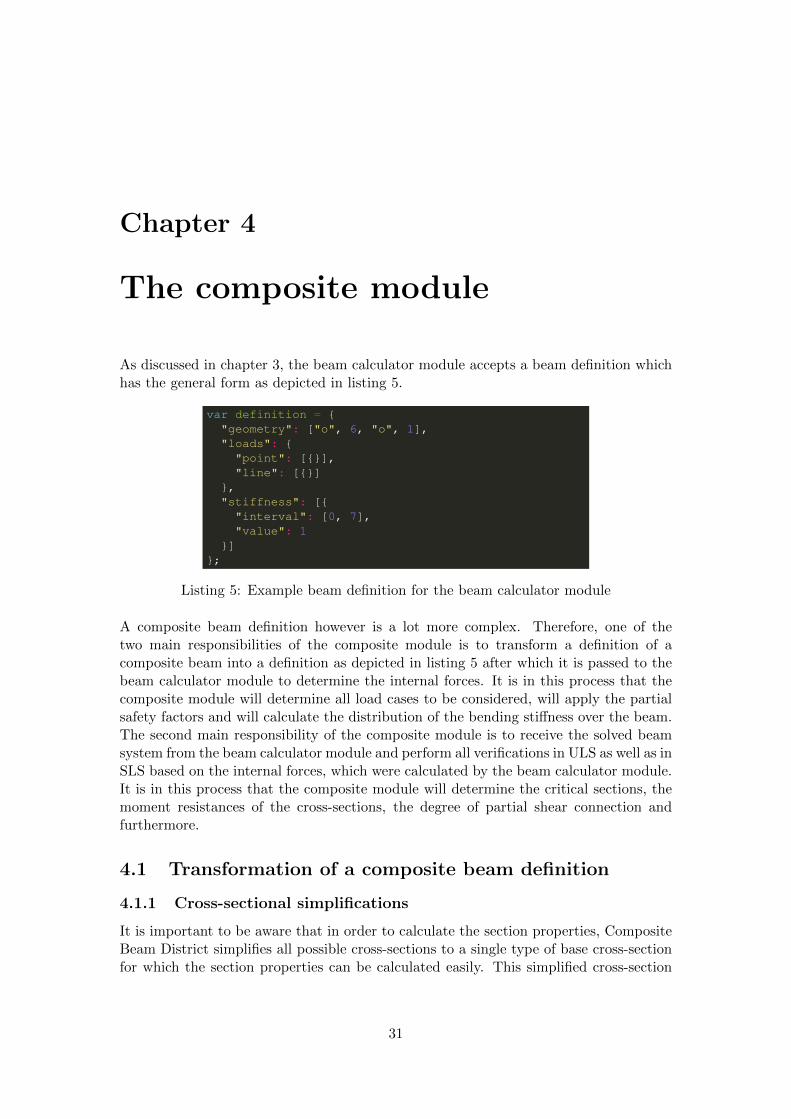
As discussed in chapter 3, the beam calculator module accepts a beam definition whichhas the general form as depicted in listing 5.
Listing 5: Example beam definition for the beam calculator module
A composite beam definition however is a lot more complex. Therefore, one of thetwo main responsibilities of the composite module is to transform a definition of acomposite beam into a definition as depicted in listing 5 after which it is passed to thebeam calculator module to determine the internal forces. It is in this process that thecomposite module will determine all load cases to be considered, will apply the partialsafety factors and will calculate the distribution of the bending stiffness over the beam.The second main responsibility of the composite module is to receive the solved beamsystem from the beam calculator module and perform all verifications in ULS as well as inSLS based on the internal forces, which were calculated by the beam calculator module.It is in this process that the composite module will determine the critical sections, themoment resistances of the cross-sections, the degree of partial shear connection andfurthermore.
4.1 Transformation of a composite beam definition
4.1.1 Cross-sectional simplifications
It is important to be aware that in order to calculate the section properties, CompositeBeam District simplifies all possible cross-sections to a single type of base cross-sectionfor which the section properties can be calculated easily. This simplified cross-section
31
consists out of a set of rectangular steel plates which represent the steel profile withouttaking into account any welds or roundings.Joris Van Nieuwerburg studied the influence of the neglection of any welds or roundingson the moment of inertia of a steel profile (Van Nieuwerburgh, 2013) and concludedthat this results in an underestimation of the moment of inertia of 5%. In this contextany welds or roundings are neglected by Composite Beam District. Moreover, there issimply no option to specify them in the graphical user interface.On top of the steel profile, an empty space with height hp will be assumed. This willallow to take into account any profiled steel sheeting, precast panel or hollow core slabwhich may be provided in the concrete slab. On top of that “empty” space, a fullconcrete section with a height hc will be assumed to represent the remainder of theconcrete slab. A sketch of this base cross-section is depicted in figure 4.1.
hp
hc
Figure 4.1: Base cross-section
Recall that this base-cross section is only a model. In reality this “empty space” is neverpresent as a connection between the steel profile and the concrete slab always has to bepresent in order to activate the composite behavior.As mentioned supra, hp depends on whether either profiled steel sheeting, a precastpanel or a hollow core slab is present. In case of a bare slab, hp = 0. In case of a profiledsteel sheeting, hp is taken as the height of the profiled steel sheeting, even if the sheetingis oriented parallel to the heart line of the beam, in which case a constant concretesection in between the profiled steel sheeting would be present along the entire beam.In case of a precast panel, the entire height of the panel is taken as hp. For hollow coreslabs, hp is taken as the distance from the steel profile to the top of the holes. Note thatall these simplifications result in a safe approximation.
4.1.2 Load transformations
The user has the ability to enter line loads or point loads which act directly on thecomposite beam, but has the ability as well to enter surface loads acting on the concreteslab. Regarding the beam definition that has to be entered in the beam calculatormodule - as depicted in listing 5 - the surface loads have to be transformed into lineloads.The composite module assumes that in case of a set of parallel composite beams withan intermediate distance of l the surface load is transferred to the nearest beam. Assuch, if a surface load q is acting on the concrete slab, the line load on the consideredcomposite beam will be p = ql.In case the beam has a free edge on one side with a length e, the line load on the beamwill be considered as p = q (l/2 + e) where l still is the intermediate distance betweenthe beams. If the beam has free edges at both sides the line load is p = q (e1 + e2) where
32
e1 and e2 represent the distances to the free edges on both sides of the beam. The zonein which the loads are carried to a certain beam will be appointed as the “influencezone” of the beam.Additionally, the composite module automatically calculates the dead weight of thecomposite beam as well. The dead weight of the slab is calculated as
gs = ρc ·Ac
where ρc is the density of the concrete in kN/m3 which can be specified and Ac is thesurface of the concrete within the influence zone of the beam. Note that any precastpanel or hollow core slab will be taken into account for Ac as well.The dead weight of the steel profile is simply calculated as
ga = ρa ·Aa
with ρa being the density of structural steel in kN/m3 and Aa being the total area ofthe steel profile. The total dead weight gk that is taken into account as a line load onthe beam automatically is then found as
gk = gs + ga
It is important to recall that the user does not need to specify the dead weight explicitly.
4.1.3 Load configurations
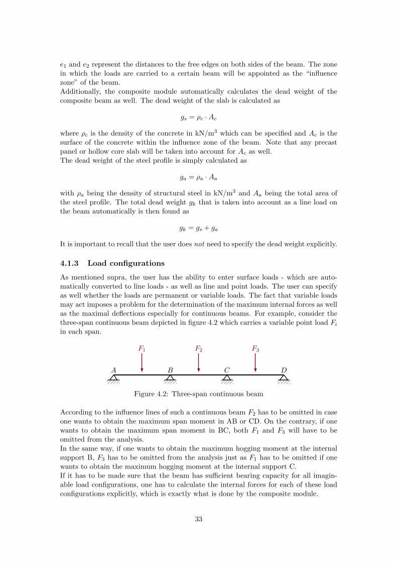
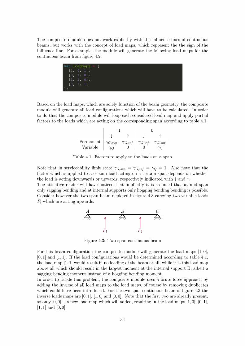
As mentioned supra, the user has the ability to enter surface loads - which are auto-matically converted to line loads - as well as line and point loads. The user can specifyas well whether the loads are permanent or variable loads. The fact that variable loadsmay act imposes a problem for the determination of the maximum internal forces as wellas the maximal deflections especially for continuous beams. For example, consider thethree-span continuous beam depicted in figure 4.2 which carries a variable point load Fiin each span.
A B C D
F1 F2 F3
Figure 4.2: Three-span continuous beam
According to the influence lines of such a continuous beam F2 has to be omitted in caseone wants to obtain the maximum span moment in AB or CD. On the contrary, if onewants to obtain the maximum span moment in BC, both F1 and F3 will have to beomitted from the analysis.In the same way, if one wants to obtain the maximum hogging moment at the internalsupport B, F3 has to be omitted from the analysis just as F1 has to be omitted if onewants to obtain the maximum hogging moment at the internal support C.If it has to be made sure that the beam has sufficient bearing capacity for all imagin-able load configurations, one has to calculate the internal forces for each of these loadconfigurations explicitly, which is exactly what is done by the composite module.
33
The composite module does not work explicitly with the influence lines of continuousbeams, but works with the concept of load maps, which represent the the sign of theinfluence line. For example, the module will generate the following load maps for thecontinuous beam from figure 4.2.
Based on the load maps, which are solely function of the beam geometry, the compositemodule will generate all load configurations which will have to be calculated. In orderto do this, the composite module will loop each considered load map and apply partialfactors to the loads which are acting on the corresponding span according to table 4.1.
1 0↓ ↑ ↓ ↑
Permanent γG,sup γG,inf γG,inf γG,sup
Variable γQ 0 0 γQ
Table 4.1: Factors to apply to the loads on a span
Note that in serviceability limit state γG,sup = γG,inf = γQ = 1. Also note that thefactor which is applied to a certain load acting on a certain span depends on whetherthe load is acting downwards or upwards, respectively indicated with ↓ and ↑.The attentive reader will have noticed that implicitly it is assumed that at mid spanonly sagging bending and at internal supports only hogging bending bending is possible.Consider however the two-span beam depicted in figure 4.3 carrying two variable loadsFi which are acting upwards.
A B C
F1 F2
Figure 4.3: Two-span continuous beam
For this beam configuration the composite module will generate the load maps [1, 0],[0, 1] and [1, 1]. If the load configurations would be determined according to table 4.1,the load map [1, 1] would result in no loading of the beam at all, while it is this load mapabove all which should result in the largest moment at the internal support B, albeit asagging bending moment instead of a hogging bending moment.In order to tackle this problem, the composite module uses a brute force approach byadding the inverse of all load maps to the load maps, of course by removing duplicateswhich could have been introduced. For the two-span continuous beam of figure 4.3 theinverse loads maps are [0, 1], [1, 0] and [0, 0]. Note that the first two are already present,so only [0, 0] is a new load map which will added, resulting in the load maps [1, 0], [0, 1],[1, 1] and [0, 0].
34
By using this brute force approach, in general, a lot of load configurations will have beenintroduced which will not introduce any critical bending moments or deflections. In orderto avoid overloading the user with a lot of results for insignificant load configurations aswell, load configurations for which the internal forces do not contain any extreme valueswill be filtered out before all verifications will be carried out. For more informationabout this filtering process, the reader is referred to 4.2.1.The writer is aware of the fact that loads which are acting upwards are very unlikely tooccur in real life situations in buildings. Nevertheless this is implemented for the sakeof universal applicability of Composite Beam District.
4.1.4 Effective width of a concrete flange
According to EN 1994-1-1:2004 5.4.1.2 (1) Composite Beam District takes into accountthe effects of shear lag in the concrete flange by defining an effective width of the concreteslab which will be taken into account for the determination of the properties of the cross-section. The effective width beff is determined according to EN 1994-1-1:2004 5.4.1.2(5) which states that
beff = b0 +∑
bei (4.1)
where b0 is the distance between the centres of the outstand shear connectors and beiis the effective width of the concrete flange on each side of the web, as also depicted infigure 4.4.
Figure 4.4: Effective width beff of a concrete flange, extracted from EN 1994-1-1:2004
bei is taken as Le/8 but of course not greater than the geometric width bi, where bi istaken as the distance from the outstand shear connector to the mid point between thewebs of two adjacent beams. If the beam is an edge beam - either on one side or onboth sides - bi should be taken as the distance from the outstand shear connector to thefree edge.Le is taken as the distance between points of zero bending moment. According to EN1994-1-1:2004 5.4.1.2 (5), one may assume Le according to figure 5.1 of EN 1994-1-1:2004.While this is practical for hand calculations, Composite Beam District determines Leusing an iterative calculation. At first, after the loads have been parsed, the compositebeam is entered in the beam calculator module with a constant bending stiffness EI = 11 after which the so called “moment zones” are requested from the analyzer. These“moment zones” contain the intervals where the bending moment has a constant signand as such they contain Le as well.
1One may recall from structural analysis that for continuous beams the absolute value of the bendingstiffness EI does not influence the internal forces as only the relative bending stiffness is of importance.As such one can safely use a bending stiffness EI = 1 for the first iteration.
35
After all values of Le have been determined, beff is determined according to (4.1) afterwhich for each moment interval the bending stiffness EI is calculated cfr. infra. Inthe calculation of EI the sign of the acting bending moment is taken into account aswell. As such the effects of cracking of the concrete on the internal forces are taken intoaccount as well, which is required according to EN 1994-1-1:2004 5.4.2.1 (1).With the initial distribution of EI over the beam, the composite beam is recalculatedby the beam calculator module after which the “moment zones” are calculated againand a new distribution of EI over the beam is determined. This procedure is repeateduntil sufficient convergence is found. Arbitrary, Composite Beam District considersthe moment zones to have sufficiently converged if the bounds of the moment zones initeration i do not differ more than 1% than those of iteration i − 1. Simulations showthat this is the case after approximately 3 a 4 iterations.After sufficient convergence of the moment zones has been found, the internal forcescorresponding to the last iteration are considered as the actual internal forces. Forthese internal forces, beff is calculated one more time for each moment zone. This willthen be the value that will be taken into account for the properties off the cross-sectionsuch as the moment resistance and so on.
4.1.5 Bending stiffness EI of a composite beam
Positive bending
The bending stiffness EI of a composite beam in a moment zone of positive bending isdetermined by using the concept of a fictive steel section. This implies that the concreteslab is transformed to a fictive steel section with a width of beff /nL with
nL =EaEc
the ratio of the modulus of elasticity of construction steel Ea and the modulus of elas-ticity of concrete Ec. Note that this allows to take into account the effects of creepand shrinkage of the concrete on the internal forces, which is required according to EN1994-1-1:2004 5.4.2.2 which is also stating that
nL = n0 (1 + ψL · ϕt)
where n0 is the modular ratio Ea/Ecm for short-term loading according to EN 1992-1-1,ϕt is the creep coefficient and ψL is the creep multiplier. The parameter nL is indeed afundamental parameter which has to be specified by the user in the tab General settingsof the user interface cfr. infra.For the obtained fictive steel section, the position of the elastic neutral axis xel is simplydetermined as
xel = xG =SfA
(4.2)
where Sf is the first moment of area of the fictive steel section and Af is the areaof the fictive steel section. Recall that the calculation of both Sf and Af is basedon the simplified “base cross-section” as was explained in 4.1.1. Also note that theapproach using the fictive steel section to determine the location of xel is equivalent tothe approach used in beams of reinforced concrete, stating that the neutral axis goesthrough the centroid of the fictive concrete cross-section (Taerwe, 2012).
36
In principle, if it turns out that xel is located in the concrete slab, part of the concretewill be in compression and part of the concrete will be in tension which would imply thatit has to be neglected introducing the need for an iterative calculation of xel. However,since neglecting the concrete in tension only has a small influence (Maquoi et al., 2012),Composite Beam District calculates the location of xel based on the uncracked cross-section.Once the location of xel is known, the moment of inertia of the fictive steel section I+fis calculated using parallel axis theorem2 as
I+f =∑i
(bi · h3i
12+ bi · hi · ~di (xel)
)+beff · h3c12 · nL
+beff
nL· hc · ~d (xel)
where ~di(xel) is the distance of the centroid of the considered steel plate to the locationof the neutral axis xel. Once If is known, the bending stiffness EI of the compositebeam is calculated as
EI + = Ea · I+fNote that any reinforcement which may be present in the concrete slab is not taken intoaccount for positive bending.
Negative bending
In case of negative bending, the concrete slab is assumed to be fully cracked and istherefore not taken into account. Again, if it would turn out that xel is located in theconcrete slab, at least a part of the concrete slab will still be subject to compression.In the same way as for positive bending, this influence is neglected and the concrete isassumed to be fully cracked.On the contrary, any reinforcement present will be taken into account, however in thecalculation of Sf the circular shape of the reinforcement is not taken into account and thearea of the reinforcement is assumed to be concentrated in the centroid. Additionally,only reinforcement bars which are located within the bounds of beff are taken intoaccount. If nr bars are located within the bounds of beff , Sf is calculated as
Sf = nr ·As · cs +∑i
bi · hi · ~d0,i
with cs being the distance from the centroid of the reinforcement to the top of theconcrete slab, As the area of one reinforcement bar, bi and hi the width respectivelyheight of steel plate i and ~d0,i the distance of centroid of steel plate i to the top of theconcrete slab.Subsequently, xel is calculated according to (4.2) after which I−f is calculated as
I−f =∑i
(bi · h3i
12+ bi · hi · ~di (xel)
)+ nr ·As · (cs − xel)2
Subsequently EI− is found analogously as
EI− = Ea · I−f2In Dutch this is known as De stelling van Steiner.
37
4.1.6 Type of analysis
The attentive reader will have noticed that the type of analysis that is implicitly used isa global linear elastic analysis as the Direct Stiffness Method which is used by the beamcalculator module is a linear elastic method. This type of analysis is an accordance withEN 1994-1-1:2004 5.4.1.1 (1) stating that “action effects may be calculated by elasticglobal analysis, even where the resistance of a cross-section is based on its plastic ornon-linear resistance”.In fact, clause 5.4.1.1 (1) of EN 1994-1-1:2004 is exactly what happens in CompositeBeam District: global linear elastic analysis is used in order to calculate the internalforces and the resistance of the cross-sections is verified according to plastic theory, atleast if allowed by the classification of the cross-section cfr. infra.
4.2 Processing of the results
As mentioned supra the composite module has two main responsibilities: transform thecomposite beam definition such that the internal forces can be calculated by the beamcalculator module and process the results by effectuating a set of verifications, both inultimate limit state as well as in serviceability limit state.The processing of the results happens - both for ULS and SLS - in two separate phases.First of all the insignificant results are filtered out, as is described 4.2.1. For each of thesefiltered results all verifications in ULS and SLS are effectuated. For the effectuation ofthese verifications the reader is referred to respectively chapter 5 and 6.
4.2.1 Filtering of insignificant load configurations
As mentioned in 4.1.3 the brute force approach to generate all possible load configura-tions may result in a sprawl of solved load configurations for which the internal forcesmay be not extreme. As such this could result in an overload of insignificant resultswhich are shown to the user.Since Composite Beam District aims to be as user friendly as possible, these insignificantresults are filtered out prior to effectuating the verifications in both ULS and SLS. Assuch only the most relevant load configurations are shown to the user. As a consequencethe user can be confident that for each load configuration that has passed the filter atleast at one location a value of an internal force is reached that is never reached in theother load configurations.
Ultimate limit state
In ULS an insignificant load configuration is defined as a configuration for which thebending moment reaches at no location a value which is larger in absolute value thanfor all other load configurations. In terms of moment envelopes one could state thatthe moment line of an insignificant result is completely contained within the momentenvelope of all load configurations. A few examples will be elaborated in order toillustrate this filtering process for ULS.
Example 4.2.1. Consider the statically determinate beam depicted in figure 4.5a witha main span of 3 m and a cantilevering part of 1 m which carries a downwards actingpermanent load of 5 kN at it’s end. The dead weight of the beam is 0.8 kN/m.
38
According to 4.1.3 the composite module will generate four load maps: [1, 0], [0, 1], [1, 1]and [0, 0], for which all moment lines are depicted in respectively figure 4.5b, 4.5c, 4.5dand 4.5e.
5 kN
3 m 1 m
(a) Loads
(b) [1, 0] (c) [0, 1] (d) [1, 1] (e) [0, 0]
Figure 4.5: Cantilever with a point load
One will notice immediately that the entire beam is subject to hogging bending for allload configurations. As such, it would be irrelevant to show the results of all four loadconfigurations to the user. Only the load configuration corresponding to [1, 1] will bewithheld as this results in the largest hogging bending moment being 7.3 kNm at theright support.
Example 4.2.2. Consider once again the cantilever of example 4.2.1 with the differencethat the permanent point load of 5 kN is now a permanent point load of 1 kN. Obviouslythe load maps stay the same, but more interesting are the moment lines, which aredepicted in figure 4.6.
(a) [1, 0] (b) [0, 1] (c) [1, 1] (d) [0, 0]
Figure 4.6: Moment lines for a point load of 1 kN
In this case the beam is subject to hogging bending as well as sagging bending. How-ever, the load configuration resulting in the maximum hogging bending moment - i.e.[1, 1] - does not coincide with the load configuration resulting in the maximum saggingbending moment - i.e. [1, 0]. As a result, the filtering process will filter out both loadconfigurations [0, 1] and [0, 0] as they don’t result in an extreme value of the bendingmoment.Important to bear in mind though is that even as load configuration [1, 0] results in alarger sagging bending moment than [0, 1], the zone with sagging bending moments willbe smaller for load configuration [0, 1] than for [1, 0]. According to 4.1.4 this also yields
39
that the effective width beff may be smaller than for load configuration [1, 0] which mayresult in a smaller moment resistance MRd as well, cfr. infra.Due to this, it is theoretically possible that even though load configuration [0, 1] yields asmaller sagging bending moment than [1, 0] it will still be more critical due to a reducedvalue of beff and consequently MRd. While not studied in detail, it is in the author’sbelief that the probability of this event is negligible.
Examples 4.2.1 and 4.2.2 show why the brute force approach of explicitly calculatingalmost all load configurations is necessary. Even though the “beam morphology”3 ofboth examples is exactly the same, it is practically impossible to determine in advancewhich load configurations will result in extreme values without explicitly calculating allimaginable load configurations.The attentive reader will probably wonder how the composite module treats load configu-rations which result in multiple regions of sagging or hogging bending. The implementedprocedure is illustrated in example 4.2.3.
Example 4.2.3. Consider the two-span continuous beams depicted in figure 4.7. Thebeam carries a variable point load of 5 kN at the middle of the first span and a variableuniformly distributed load of 2 kN/m over the first span. Additionally the beam carriesit’s dead weight of 0.8 kN/m which is by definition a permanent load.
5 kN
2 kN/m
4 m 2 m
Figure 4.7: Two-span continuous beam carrying a point load and a line load
Once again, four load maps [1, 0], [0, 1], [1, 1] and [0, 0] are constructed which result inthe moment lines depicted in figure 4.8.
(a) [1, 0] (b) [0, 1] (c) [1, 1] (d) [0, 0]
Figure 4.8: Moment lines for all load configurations of figure 4.7
From the moment lines depicted in figure 4.7 one deduces that the load configuration[1, 0] results in a zone of sagging bending and a zone of hogging bending, while the loadconfigurations [0, 1], [1, 1] and [0, 0] all result in two zones of sagging bending and a zoneof hogging bending at the internal support.
3The expression “beam morphology” has to be understood in the sense that the general configurationis the same. Both beams are simply supported beams with a cantilevering part, and both beamscarry a uniformly distributed load over their entire length as well as a point load at the end of thecantilever. Regardless of the values of the loads and the span lengths, both beams can be considered as“morphologically equal”.
40
The composite module will now classify the different moment lines that are encountered.The moment line from load configuration [1, 0], which is depicted in figure 4.8a, can becharacterized by the fact that it contains a zone of sagging bending followed by a zoneof hogging bending. In case sagging bending is denoted as 1 and hogging bending isdenoted as 0, the moment line can be classified as 10, which using the binary numbersystem could be seen as the decimal number 2. Likewise, the moment lines of the loadconfigurations [0, 1], [1, 1] and [0, 0] are classified as 101 or 5.Subsequently the composite module loops all “classes” of moment lines for which it loopsall zones of each moment line in the class. Each load configuration which results in anextreme value of the bending moment in a zone will pass the filter.Applied to the present example, the composite module will first consider all momentlines of class 2. Only the moment line corresponding to load configuration [1, 0] is of class2, so load configuration [1, 0] will pass the filter anyway. Class 5 contains three momentlines however. The maximum value for the first zone of sagging bending is obtained byload configuration [1, 1] as clearly visible on figure 4.8c. The maximum value for thezone of hogging bending around the internal support is obtained by load configuration[1, 1] as well. For the second zone of sagging bending the maximum value is obtainedby load configuration [0, 1]. As such, load configurations [1, 0], [0, 1] and [1, 1] will passthe filter and will be shown to the user.
Serviceability limit state
The filtering of insignificant load configurations in serviceability limit state is intimatelyintertwined with the verifications carried out for the deflections. Hence the reader isreferred to 6.3.
4.2.2 Verifications in ultimate limit state
After the internal forces have been been calculated for all load configurations and afterthe insignificant load configurations have been filtered out, the composite module willverify whether the bearing capacity of the composite beam is sufficient for the actinginternal forces. For the actual effectuation of the verifications the reader is referred tochapter 5.
4.2.3 Verifications in serviceability limit state
In serviceability limit state, the main verification carried out is the verification of themaximum total deflections as well as the maximum additional deflections due to thevariable loads. For the detailed explanation the reader is referred to chapter 6.
41
Chapter 5
Ultimate limit state
5.1 Critical sections
In principle, the basic equation of the method of the limit states
E ≤ R (5.1)
has to be satisfied for each imaginable point of the composite beam. This is of coursevery impractical to work with, if it even were possible. Therefore one resorts to so calledcritical sections for the ultimate limit state. These critical sections are cross-sectionswhere one of the action effects, such as bending moment or vertical shear force will beextreme.As such, if the critical sections are well-chosen and all verifications of the type (5.1)are fulfilled for each critical section, one may assume the composite beam to be able towithstand the loads in ultimate limit state.As mentioned before, a computer is not able to make real “thoughtful” choices. There-fore, a robust algorithm is needed in order to find the appropriate critical sections forany imaginable composite beam with any load configuration.The basic philosophy behind the algorithm that was implemented in the compositemodule to find all critical sections is that each moment zone of the beam as describedin 3.3.4 has constant cross-sectional properties due to a constant effective width beff
as described in chapter 4. As such, for each moment zone, the cross-sections with thelargest acting bending moment - both negative and positive - as well as the largest actingshear force will be determined.The maximum moments and maximum shear force can be easily obtained for eachelement using the analyzer as described in 3.3.2 and 3.3.3. However, all elements whichare - at least partly - contained within a certain longitudinal section of the beam stillneed to be found. In order to do this, the interval tree of all elements of the beam thatwas constructed by the analyzer as explained in 3.3.2 is used. As mentioned as well in3.3.2, an interval tree is not only capable of finding all intervals that contain a givenpoint, but is capable of finding all intervals that are overlapping with a given intervalas well.Using this capability, the composite module queries the interval tree for all elements thatare overlapping with each moment zone. Using the analyzer, the maximal values of theshear force and the bending moment over all elements can be found. The correspondingcross-sections are then the critical sections for the considered moment zone. As such allcritical sections over the entire beam can be determined.
42
Note that EN 1994-1-1:2004 6.1.1(4) defines critical sections to include
- Sections of maximum bending moment;
- Supports;
- Sections subject to concentrated loads or reactions;
- Places where a sudden change of cross-section occurs, other than a change due tocracking of concrete;
The algorithm elaborated above naturally includes sections of maximum bending mo-ment. Supports will often naturally be included due to the fact that the largest verticalshear force will often be present here, or in case of internal supports the largest hoggingmoment. However, theoretically one could find a load configuration where the supportsare not subjected to extremal moments or vertical shear forces, causing them to beomitted from the critical sections.One could argue that this is not an issue since other critical sections in the longitudinalbeam section would “supersede” the support such that if the other critical section passesall verifications, the support would as well due to the fact that smaller load effects act inthe support than in the other critical section, while both still have the same resistanceproperties due to them being in the same moment zone. This would be true, if thevertical shear resistance and the moment resistance would be independent. This is notthe case since interaction between both has to be taken into account, cfr. infra.In order to overcome this issue, all supports are explicitly added to the critical sectionsafter they have been determined by the algorithm in order to be 100% sure that theyare included. The same approach is applied to cross-sections with concentrated loads.Note that places where a sudden change of cross-section occurs are out of the scope ofthe composite module since it is only possible to specify one cross-section over the entirelength of the composite beam.
5.2 Vertical shear
In each critical section, a certain amount of verifications of the type
E ≤ R (5.1)
has to be carried out. One of these verifications is the resistance to vertical shear.According to EN 1994-1-1:2004 6.2.2 the resistance to vertical shear Vpl,Rd is taken asthe plastic shear resistance of Vpl,a,Rd of the steel section only. Vpl,a,Rd is determined inaccordance with EN 1993-1-1 6.2.6 stating that
Vpl,a,Rd =Avfy
γM0
√3
where Av is the shear area. For reasons of simplicity, Av is taken as the area of the web,being
Av = tw · hwAs such the resistance to vertical shear is verified as
VEd ≤ Vpl,Rd
Note that the verification for shear buckling of the web is not taken into account.
43
5.3 Bending resistance
According to EN 1994-1-1:2004 6.2.1.1, the resistance moment of the composite cross-section is determined using rigid-plastic theory in case the cross-section is in Class 1 orClass 2. The resistance moment of cross-sections in Class 3 is determined using elastictheory. Class 4 cross-sections are out of the scope of Composite Beam District and assuch Composite Beam District will display an error message if a cross-section was foundto be in Class 4.The classification system for composite cross-sections is the same as the system for puresteel sections as defined in EN 1993-1-1 5.5.2, with the difference that upper flanges incompression are assumed to be restrained from buckling due to their attachment to theconcrete slab by means of shear connectors and therefore are always Class 1.
5.3.1 Plastic resistance moment
For cross-sections in Class 1 or Class 2, the resistance moment is determined using rigid-plastic theory and in accordance with EN 1994-1-1:2004 6.2.1.2. A typical plastic stressdistribution is depicted in figure 5.1.
Figure 5.1: Example plastic stress distribution, extracted from EN 1994-1-1:2004
The procedure to determine the plastic resistance moment Mpl is pretty straightforward,however, one should take into account that the tensile strength of concrete is neglected,which is in accordance with EN 1994-1-1:2004 6.2.1.1(4). Note that the stresses actingin the concrete are not taken to equal the design compressive strength fcd, but rather0.85fcd which is in accordance with EN 1994-1-1:2004 6.2.1.2(1).A fundamental parameter in the determination of the plastic resistance moment is thelocation of the plastic neutral axis xpl, which is by convention calculated starting fromthe top of the concrete slab. This does not only determine the plastic resistance moment,but is of importance for the determination of the Class of the cross-section as well.For positive bending one may verify that xpl is located in the concrete slab if
Na < 0.85fcd · hc · beff (5.2)
where Na is the total normal force that the steel profile is able to take up, hc is theeffective height of the concrete slab and beff is the effective width of the concrete slab.In most cases Na will equal Aa · fyd where Aa is the total area of the steel profile andfyd is the design steel strength. However, in order to be able to take into account theinfluence of vertical shear on the bending resistance (cfr. infra), the composite moduleexplicitly calculates Na as
Na =∑i
bi · hi · fyd,i
44
where bi, hi and fyd,i respectively represent the width, the height and the design steelstrength of each plate of the steel profile.If (5.2) is fulfilled, xpl is located in the concrete slab and is given by
xpl =Na
0.85 · beff · fcd
If (5.2) is not fulfilled, the concrete slab fully acts in compression and xpl is locatedin the steel profile after which xpl can be obtained by expressing that the resultingnormal force should be 0 which is done in the composite module by a progressive searchalgorithm. Initially, the total normal force in the cross-section if all elements would reachtheir design strengths is calculated. Subsequently the algorithm progressively loops allelements - both concrete slab and steel plates - from top to bottom and adds up theircontributions. If the sum of the contributions exceeds half of the total normal forcecalculated earlier, the element where xpl is located is found. From then on, xpl can beeasily calculated by expressing that the total normal force above xpl should equal thetotal force below xpl.Once xpl is located, the total resistance moment can be easily calculated by addingup the contribution to the total moment of each element, both concrete slab and steelplate, around xpl. Note that if xpl is located in one of the steel plates, this plate has twocontributions: a contribution in tension and a contribution in compression. Note thatany tensile reinforcement in the concrete slab is neglected.For negative bending the calculation of the plastic moment resistance happens in asimilar way, however the concrete is now assumed to be fully cracked. Although sometensile reinforcement will be present which in theory may cause xpl to be located in theconcrete slab, the concrete slab will always be assumed to be fully cracked. xpl willonly be located in the concrete slab in case of extremely high reinforcement ratios incombination with an extremely small steel profile. In practice this will never be the case,which is why this case is left out and xpl is assumed to be located in the steel profile.Since xpl is located in the steel profile, the same algorithm as for positive bending can befollowed, however taking into account the tensile reinforcement instead of the concreteslab. Apart from this, the calculation is not fundamentally different.In case structural steel grade S420 or S460 is used, a reduction factor β is applied to theplastic resistance moment in case the ratio xpl/h > 0.15 where h is the total height ofthe cross-section. The reduction factor β is depicted in figure 5.2. This is in accordancewith EN 1994-1-1:2004 6.2.1.2 (2).
Figure 5.2: Reduction factor β, extracted from EN 1994-1-1:2004
In case xpl/h > 0.4, EN 1994-1-1:2004 6.2.1.2 (2) specifies that the calculation of theresistance moment should be carried out using non-linear theory. This is out of thescope of Composite Beam District and it will therefore display an error message.
45
5.3.2 Elastic resistance moment
In order to determine the elastic resistance moment of a composite cross-section, thenotorious formula
σ =My
I(5.3)
is used. The moment of inertia I has to be taken as the moment of inertia of the fictivesteel section, as was elaborated in 4.1.5. Recall that it’s value will depend on whetherhogging or sagging bending moments are acting. In accordance with EN 1994-1-1:20046.2.1.5 (2), three limiting stresses for σ apply:
- fyd: The stress in the bottom fibre of the lower bottom flange of the steel profilemay not exceed the design yield stress fyd of the structural steel;
- fcd: In case of a positive bending moment, which results in the concrete slab actingin compression, the stress at the top fibre of the concrete slab may not exceed thedesign compressive strength fcd of the concrete;
- fsd: In case of a negative bending moment, the stress in any tensile reinforcementmay not exceed the design yield stress fsd of the reinforcement.
Note that that in order for σ in expression (5.3) to yield concrete stresses, the momentof inertia I that is entered has to be the moment of inertia of the concrete section Ic,rather than that of the fictive steel section If . If one recalls that at the same fibre, thesteel stress will be nL times the concrete stress, Ic is found as
Ic = nL · If
Summarized one can state that the elastic resistance moment Mel,Rd is to be taken asthe minimum of
Ma =fyd · Ifh− xel
Mc =fcd · nL · If
xelMs =
fsd · Ifxel − cs
(5.4)
of course only considering Mc in case of a positive acting bending moment and Ms incase of a negative acting bending moment. In (5.4), h represents the entire height ofthe composite cross-section, calculated from the top fibre of the concrete flange to thebottom fibre of the steel profile, xel is the location of the elastic neutral axis, takenfrom the top fibre of the concrete flange and calculated as elaborated in 4.1.5 and cs isthe location of the centroid of the tensile reinforcement, taken from the top fibre of theconcrete flange.
5.3.3 Bending and vertical shear
EN 1994-1-1:2004 6.2.2.4 requires the effect of vertical shear to be taken into account ifthe vertical shear force VEd exceeds half of the shear resistance VRd.For composite cross-sections in Class 1 or Class 2 the composite module takes the in-fluence of vertical shear into account as proposed in EN 1994-1-1:2004 6.2.2.4 (2) byapplying a reduced design steel strength (1 − ρ)fyd in the web when calculating theplastic resistance moment where ρ is given by
ρ =
(2VEdVRd
− 1
)2
46
Note that ρ ≤ 1 as the profile would fail in vertical shear if ρ > 1.The procedure of applying a reduced design steel strength to the web is schematicallyrepresented in figure 5.3. It requires no significant changes to the method elaborated in5.3.1 which calculates Mpl,Rd.
Figure 5.3: Influence of vertical shear on the resistance moment, extracted from EN1994-1-1:2004
For cross-sections in Class 3 no interaction between bending and shear is taken intoaccount.
5.4 Longitudinal shear
5.4.1 Degree of shear connection η
An important concept for composite beams is the degree of shear connection η. Theplastic resistance moment Mpl,Rd of the full composite cross-section as elaborated in5.3.1 can only be established if a full shear connection at the interface between the steelsection and the concrete slab is provided.To take into account the use of partial shear connections, the composite module uses theconservative, simplified method proposed in EN 1994-1-1:2004 6.2.1.3 (5) to determinethe moment resistance MRd, which corresponds to line 2 in figure 5.4.
Figure 5.4: Relation between MRd and η, extracted from EN 1994-1-1:2004
According to this simplified method the composite module will in this case apply areduction on the plastic resistance moment of the composite cross-section according to
MRd = Mpl,a,Rd + (Mpl,Rd −Mpl,a,Rd) η (5.5)
where Mpl,a,Rd is the plastic resistance moment of the steel profile and Mpl,Rd is the fullplastic resistance moment of the entire composite cross-section, as elaborated in 5.3.1.
47
Note that both for Mpl,a,Rd as for Mpl,Rd the influence of vertical shear is taken intoaccount in the way that was elaborated in 5.3.3.In order to know the degree of shear connection η the composite beam is subdividedin several zones of longitudinal shear. Each zone has a certain longitudinal shear forceVl,Rd assigned to it which represents the shear force that has to be taken up at theinterface between the steel profile and the concrete slab in case the full plastic capacityof the composite beam would be used.It is important to note that Vl,Rd is not present in reality. It simply represents thelongitudinal shear force that would be present if the full plastic plastic capacity of thecomposite beam would be used. If this Vl,Rd can actually be taken up by the shear con-nectors, this indicates that the full plastic capacity of the composite beam can actuallybe used. Note that this is also reflected by (5.5) for η = 1.Based on the above, the degree of partial shear connection η will be calculated as
η =VP,RdVl,Rd
≤ 1
where VP,Rd is the total shear force that can be taken up by all shear connectors presentin the considered zone of longitudinal shear. Conceptually, one could write
VP,Rd =∑i
PRd,i
with PRd,i being the resistance of an individual stud connector and where the summationhas to be taken over all shear connectors in the considered zone of longitudinal shear.Note that if no shear connectors would be present, η = 0, so that according to (5.5) themoment resistance of the composite beam entirely originates from the steel profile. Thebeam acts as a traditional steel beam and all composite action is lost. This emphasizesthe importance of the shear connectors in order to establish composite action.Only one type of shear connectors can be entered in Composite Beam District, beingheaded stud connectors. The resistance of these stud connectors is calculated accordingto EN 1994-1-1:2004 6.6.3.1 and is given by the minimum of
PRd =0.8 · fu · π·d
2
4
γv
and
PRd =0.29 · α · d2
√fck · Ecm
γv
which respectively reflect failure of the stud connector itself and failure of the concretearound the stud connector. fu is the specified ultimate tensile strength of the material ofthe stud, but not greater than 500 N/mm2, fck is the characteristic cylinder compressivestrength of concrete and γv is the partial safety factor. The factor α has to be taken as
α = 0.2
(hscd
+ 1
)for 3 ≤ hsc
d≤ 4
α = 1 forhscd
> 4
with hsc being the overall height of the stud.In case a profiled steel sheeting is used as depicted in figure 5.5, a reduction factor hasto be applied to PRd according to EN 1994-1-1:2004 6.6.4. For the calculation of the
48
Figure 5.5: Profiled steel sheeting with stud connectors, extracted from EN 1994-1-1:2004
reduction factors which is also implemented by Composite Beam District a reference ismade to EN 1994-1-1:2004 6.6.4.An important part which has not been treated yet, is the determination of the shearzones and their corresponding values of Vl,Rd. EN 1994-1-1:2004 does not provide specificdetails on how to determine these parameters, however, a zone of longitudinal shearshould be considered as the zone over which an acting Vl,Rd is “spread”, as conceptuallydepicted in figure 5.6.
Figure 5.6: Spreading of Vl,Rd (Maquoi et al., 2012)
According to Maquoi (Maquoi et al., 2012) the zones of longitudinal shear are the zonesbetween the critical sections or equivalently the zones between extremal moments andpoints where important point loads are acting. Hence the length of such a zone is alsoindicated as critical length lcr.The value of Vl,Rd acting in each zone of longitudinal shear can be obtained by anequilibrium consideration. Consider a freed zone of longitudinal shear as depicted infigure 5.7 where the cross-section has been cut above the steel profile at the interfacebetween the concrete and the steel profile, also indicated as II in figure 5.6.
Ml Mr
Vl,Rd
Nl Nrlcr
Figure 5.7: Freed zone of longitudinal shear
At the ends of the zone, the plastic bending moments are considered as the desired Vl,Rdis the longitudinal shear force that has to be taken up in case the full plastic capacityof the composite beam is used. Both moments introduce a plastic stress distributionat the ends as depicted in figure 5.1. Due to the cut at the interface the resultant ofthe stress distribution will not be zero and hence a normal force at the ends will act.Consequently, at the interface a longitudinal shear force Vl,Rd needs to be present inorder to keep the zone in equilibrium.
49
If the moments are sagging, respectively hogging bending moments, N is found as
N+ = Aa · fyd ≤ 0.85 · fcd · hcN− = − As · fsd
where the sign of N is in accordance with the sign convention of figure 5.7. The upperbound for N+ is valid if xpl is located in the steel profile. If one of the ends of the zonecorresponds to a bending moment of zero obviously no normal force N will act on thezone.Vl,Rd is now obtained by expressing the horizontal equilibrium of the freed zone oflongitudinal shear as
Vl,Rd = Nr −Nl
Note that the sign of Vl,Rd is not of importance.Also note that in case the zone of longitudinal shear is entirely contained in a zone wherethe bending moment has a constant sign, Vl,Rd will be zero. At first glance this mayseem strange. A few examples will be elaborated in order to clarify this and to highlightsome other issues.
Example 5.4.1. Consider the simply supported beam depicted in figure 5.8 carrying aline load of 1 kN/m and two point loads at the respective offsets 1 m and 3 m.
Figure 5.8: Load configuration
The moment line and the shear line for this configuration are depicted in respectivelyfigure 5.9a and 5.9b.
(a) Moment line (b) Shear line
Figure 5.9: Moment and shear line for example 5.4.1
According to the definition of critical sections, this beam configuration contains fivecritical sections: two at the supports, two at the point loads and one at mid-span wherethe bending moment is maximal. Each zone has a length lcr = 1 m. In accordance towhat was elaborated above, Vl,Rd in the zones between the point loads will be zero. Thiswould indicate that no shear connectors are required to fully use the plastic momentcapacity of the composite in these zones.However, in the zones between a support and a point load Vl,Rd will be found as
Vl,Rd = Aa · fyd ≤ 0.85 · fcd · hc · beff
50
One can compare this to the case where only a uniformly distributed load is present.This case yields two zones of longitudinal shear with lcr = 2 m which have to take upthe very same Vl,Rd. One can conclude that even though the longitudinal shear forceVl,Rd is exactly the same, it will have to be taken up in a zone with a smaller length lcrfor the case with point loads than for the case with a simple line load.
Example 5.4.2. Consider the load configuration for a continuous composite beam asdepicted in figure 5.10.
Figure 5.10: Example continuous composite beam
The moment line as well as the shear line for this configuration are depicted in figure5.11. One finds 6 zones of longitudinal shear, all indicated as well in figure 5.11.
(a) Moment line
(b) Shear line
Figure 5.11: Moment and shear line for example 5.4.2
For zones 1 and 6 one obtains
Vl,Rd = Aa · fyd ≤ 0.85 · fcd · hc · beff
Zones 2, 3, 4 and 5 are all respectively subject to both hogging bending and saggingbending and one obtains
Vl,Rd = Aa · fyd +As · fsd ≤ 0.85 · fcd · hc · beff +As · fsd
Recall that the effective width beff has to be taken as the effective width at that locationas was based on the moment zones as elaborated in 4.1.4.
Example 5.4.3. Consider once again the simply supported beam of example 5.4.1however with an additional point load of 8 kN acting as mid-span which is depicted infigure 5.12.
51
Figure 5.12: Load configuration
The corresponding moment and shear line are depicted in respectively figure 5.13a and5.13b. As expected one finds once again four zones of longitudinal shear with thesupports as well as the locations of the point loads as boundaries.
(a) Moment line (b) Shear line
Figure 5.13: Moment and shear line for example 5.4.3
For the zones near the supports one will find the same value for Vl,Rd as for example5.4.1 and likewise one finds Vl,Rd = 0 for the zones at mid-span. According to whatwas elaborated above, regardless of the amount of shear connectors used, the full plasticmoment capacity can always be achieved at mid-span as Vl,Rd = 0 and hence η = 1.On the contrary, the full plastic moment capacity at the point loads 2 kN can only beachieved in case sufficient shear connectors are provided.Note however that from the bending moment line one obtains that at the point loadsof 2 kN MEd = 7.5 kNm where at mid-span MEd = 12 kNm. As such one can concludethat if the beam would fail in bending, it will fail at mid-span if
η >7.5
12= 0.625
and fail at the location of the point loads of 2 kN if η < 0.625 where η is the degree ofshear connection in the zones nearest to the supports.
Example 5.4.4. Consider the two-span continuous beam carrying a line load of 4 kN/mas depicted in figure 5.14.
Figure 5.14: Load configuration
The corresponding moment and shear line are depicted in respectively figure 5.15a and5.15b. Special attention has to be given to the first zone of longitudinal shear, indicatedin the blue circle in both figure 5.15a and 5.15b.Due to the small dimensions of the zone of sagging bending, the zone of longitudinalshear will be extremely small as well. This does however not yield that Vl,Rd will be
52
(a) Moment line (b) Shear line
Figure 5.15: Moment and shear line for example 5.4.4
small as well. As a consequence, only very few shear connectors can be used to take upa large value of Vl,Rd. Hence η will often be close to zero in such small zones.The fact that η is often close to 0 is almost never a problem though. η = 0 indicatesthat at failure no composite action can be taken into account, and the acting bendingmoment has to be withstood by the steel profile only.Since such small zones often never contain significant bending moments compared tothe rest of the beam - as also depicted in figure 5.15a - failure will in practice neveroccur in these zones.
The examples elaborated above try to indicate that the degree of shear connection ηthat is calculated by the composite module always has to be handled with care. It isadvisable that the engineer using Composite Beam District is fully aware of the meaningof Vl,Rd, it’s calculation and how it is related to η.
5.4.2 Limitation on the use of partial shear connections
Sagging bending
According to EN 1994-1-1:2004 6.6.1.2 a limitation has to be applied on the use of partialshear connectors. For steel sections with equal flanges the limit value
ηlim = 1− 355
fyd(0.75− 0.03 · Le) ≥ 0.4
applies in case Le ≤ 25 m, where Le is the distance between the moment zeros forsagging bending as described in 4.1.4 and ηlim = 1 in case Le > 25 m. For steel sectionshaving a bottom flange with an area equal to three times the area of the top flange thelimit value
ηlim = 1− 355
fyd(0.3− 0.015 · Le) ≥ 0.4
applies if Le ≤ 20 m and ηlim = 1 if Le > 20 m.Although EN 1994-1-1:2004 6.6.1.2 (2) only specifies that in case the bottom flangehas an area exceeding that of the top flange, but less than three times the area ofthe top flange linear interpolation may be used, the composite module will use linearinterpolation for all cases by the absence of more specific details.Furthermore, the composite module will only verify that η ≥ ηlim in case
MEd > Mpl,a,Rd
which is equivalent to stating that composite action is required to take up the actingmoment MEd as it cannot be taken up by the steel section alone. As such, small zonesof longitudinal shear - as for example encountered in example 5.4.4 - for which η willoften be smaller than ηlim will not cause the composite beam to fail the verifications aslong as MEd < Mpl,a,Rd.
53
Hogging bending
According to EN 1994-1-1:2004 6.2.1.3 (2) no partial shear connections are allowed inregions of hogging bending in order to ensure yielding of the tensile reinforcement. Assuch, 1 can be considered as ηlim in regions of hogging bending. In the same way as forpartial shear connections in regions of sagging bending, the verification that η ≥ ηlim = 1is only carried out if MEd > Mpl,a,Rd.
5.4.3 Class 3 profiles
As the attentive reader may have noticed, the concept of η heavily depends on theplasticity of composite beams. Hence, in case of a profile of Class 3, no verificationsregarding η are carried out as it is meaningless for Class 3 profiles.
5.5 Lateral-torsional buckling
EN 1994-1-1:2004 6.4 describes the procedure to follow in order to verify compositebeams for lateral-torsional buckling. Due to the fact that the upper steel flanges areattached to the concrete slab, lateral-torsional buckling must not be feared when theseflanges act in compression since they may be assumed as laterally stable. However,the bottom flanges of the steel profile are not laterally restrained and as such lateral-torsional buckling is to be feared when they act in compression. In practice, the bottomflanges will act in compression at internal supports of continuous beams.The verification of lateral-torsional buckling for continuous beams with cross-sections inClass 1, 2 or 3 is described in EN 1994-1-1:2004 6.4.3, which is the method implementedin Composite Beam District. Note that Class 4 cross-sections may not be verified ac-cording to this method, which is not an issue since Class 4 cross-sections are out of thescope of Composite Beam District.According to EN 1994-1-1:2004 6.4.2 the maximum moment due to lateral-torsionalbuckling is given by
Mb,Rd = χLTMRd
where MRd is the resistance moment of the cross-section - be it determined plasticallyor elastically - and χLT is the reduction factor for lateral-torsional buckling. Of courseMb,Rd cannot be greater than MRd causing χLT to have an upper bound of 1. Further-more, χLT is a function of the relative slenderness λLT defined as
λLT =
√MRk
Mcr
in which MRk is the resistance moment of the cross-section using the characteristicmaterial properties. Whether MRk will be determined according to plastic or elastictheory depends on the classification of the cross-section. Mcr is the elastic criticalmoment for lateral torsional buckling.From λLT, χLT is obtained as
χLT =1
φLT +√φ2LT − λ2LT
≤ 1
withφLT = 0.5
(1 + αLT
(λLT − 0.2
)+ λ2LT
)54
αLT is a factor depending on the used buckling curve, which on it’s turn depends whetherthe steel profile is rolled or welded as well as on the ratio h/b of the steel profile. Theexact values of αLT can be found in Table 6.3 of EN 1993-1-1:2005.Regarding Mcr, EN 1994-1-1:2004 does not specify how this should be calculated exactly.EN 1994-1-1:2004 does allow however to calculate Mcr based on the “continuous invertedU-frame” model for composite beams where the slab is also attached to one or moresupporting steel members. This takes into account the resistance to rotation of thetop flange due to bending of the slab and can be modelled in the calculation of Mcr asa rotational spring with constant ks present over the entire length of the beam. Theinverted U-frame model is also depicted in figure 5.16.
Figure 5.16: Inverted U-frame model, extracted from EN 1994-1-1:2004
EN 1994-1-1:2004 6.4.2 (6) defines the value of ks as
ks =k1k2k1 + k2
where k1 is the flexural stiffness of the cracked concrete slab in the direction transverseto the steel beam. k1 may be taken as
k1 = αEI2a
with α = 2 for an edge beam or α = 3 for an inner beam, EI2 is the cracked flexuralstiffness per unit width of concrete slab and a is the intermediate distance between thesteel beams, as also depicted in figure 5.16. k2 is the flexural stiffness of the steel web,which should be taken as
k2 =Eat
3w
4(1− ν2a)hs
where νa is Poisson’s ratio for structural steel. hs and tw are defined in figure 5.16.As mentioned supra, EN 1994-1-1:2004 does not specify how to calculate Mcr. It onlyspecifies that the U-frame action may be taken into account by means of ks. The formulawhich is used by Composite Beam District to determine the elastic critical moment forlateral-torsional buckling Mcr is
Mcr =π2EIzl2
√√√√√IwIz
+l2GItπ2EIz
+ksl
4
π4EIz︸ ︷︷ ︸U-frame
(5.6)
where G is the shear modulus of steel, It is the torsion constant, Iz is the moment ofinertia of the steel profile around the weak axis and Iw is the warping constant.Formula (5.6) is a modified form of the classical formula for lateral-torsional bucklingfor a simply supported beam with length l and a constant bending moment applied to italong the entire beam. The term containing ks is the term that was added to representthe U-frame action.
55
The reasoning behind (5.6) is as follows. Van Impe (Van Impe, 2013) derived a for-mula for the critical uniformly distributed load pcr for a simply supported beam with arotational spring along the beam as
pcr · l2
8=
3.612
l
(GIt · EIz +
π2
l2EIz · EIw +
((−1.465 d− 0.839 ry)
EIzl
)2
+ksl
2
π2EIz
) 12
− (1.465 d+ 0.839 ry)EIzl
(5.7)
where ry is related to the vertical asymmetry of the steel profile. d is the distancebetween the point where pcr acts and the shear center of the profile. As such, forprofiles containing two axes of symmetry, d = 0 in the same way as ry = 0. Van Impeexamines the importance of the factors ry and d and concludes that neglecting thesefactors does not result in severe errors. As such, (5.7) can be simplified to
pcr · l2
8=
3.612
l
√GIt · EIz +
π2
l2EIz · EIw +
ksl2
π2EIz (5.8)
Taking into account that the maximum span moment for a simply supported beam witha uniformly distributed load p is pl2/8, (5.8) can be further simplified to
Mcr =3.612 πEIz
l2
√IwIz
+l2GItπ2EIz
+ksl4
π4EIz(5.9)
which greatly resembles (5.6). The only difference is that π2 appears in (5.6) whereasthis factor is 3.612 π in (5.9). Van Impe already notes this and remarks that Mcr fora uniformly distributed load is 15% larger than Mcr for a beam subject to a constantbending moment. As such, (5.6) can be considered conservative since a constant bendingmoment will in practice never be present in the zone around internal supports.An important factor in (5.6) which was not treated yet, is the length l. Normallythis should be the length between the supports. However, in the context of continuousbeams, l can be taken as the length between the moment zeros, as also depicted in figure5.17.
l
Figure 5.17: Buckling length l to take into account
The reason why l has to be taken equal to the length between the moment zeros is thatthe moment zeros can be considered as lateral supports, since the bottom flanges willchange from being in compression to being in tension at these zeros, as such providinglateral restraints as flanges in tension cannot move laterally. Note that this assumptionis not entirely correct, however it is assumed to be satisfactory in order to avoid extensiveFEM calculations.In practice Composite Beam District carries out the verifications for lateral-torsionalbuckling as follows. Each longitudinal section of the beam is checked whether negative
56
moments are present. These sections will in practice be the sections above internalsupports. If negative moments are present, all normal verifications mentioned supra arecarried out, but the reduction factor χLT is applied to the bending resistance moment,where χLT is calculated as explained supra. As value for l in (5.6), the length of thesection containing the negative moments is entered.
5.5.1 Note on the construction stage
EN 1994-1-1:2004 6.4.1 (3) requires the effects of sequence of construction to be takeninto account according to EN 1993-1-1:2005 6.3.2.1-6.3.2.3 and 6.3.4. In practical termsthis means that in case of an unpropped construction stage, one has to verify whetherthe steel profile does not suffer from lateral-torsional buckling due to the dead weightof the wet concrete.In particular, this includes verifications for sagging bending as well. These verificationsare not carried out by Composite Beam District, since this only carries out verificationsfor hogging bending at internal supports. If one deems that lateral-torsional buckling ofthe steel beam has to be feared in the construction stage, one should verify this usingreadily available third-party software, such as LTBeam (CTICM, 2012).
57
Chapter 6
Serviceability limit state
In chapter 4 it was explained how the composite module uses the beam calculator moduleto obtain the internal forces in ULS of all load configurations. The composite moduleuses the beam calculator module as well to determine the deflections in SLS. However,as the calculation of the deflections is heavily intertwined with the verifications thathave to be carried out, it was not treated in detail in chapter 4 how these deflections arecalculated. As a consequence, an explanation of which verifications are carried out inSLS for the deflections will be given in 6.1 before it will be elaborated how the compositemodule actually calculates the deflections in 6.2.
6.1 Verification of the maximum vertical deflection
For the verification of the deflections, two “types” of deflections are verified as
δmax ≤l
400δ2 ≤
l
500
where δmax is the maximum vertical deflection in a span under permanent and live loadsand δ2 is the additional deflection due to live loads only and l is the span length. Incase of a cantilever, l is taken as two times the length of the cantilever. These valuesare adopted from Van Impe (Van Impe, 2011) and are valid for general beams.
6.2 Calculation of the deflections
The fact that both δmax and δ2 are required for the verification of the deflections yieldssome difficulties in the calculation of the deflections. Using a naive approach, one maycalculate the deflections originating from the permanent loads only - designated as vg(x)- and subsequently the deflections originating from the permanent and variable loads -designated as vg+q(x). Clearly δmax is obtained from vg+q(x) and δ2 can be obtainedfrom vq(x) = vg+q(x)− vg(x).The problem however is that vq(x) has to be calculated explicitly due to the fact that
max (vq(x)) 6= max (vg+q(x))−max (vg(x))
which is a consequence of the non-linearity of the deflections.The explicit calculation of vq(x) by Composite Beam District is far from trivial as thedeflections of a certain beam configuration are a concatenation of the deflections of all
58
elements in the beam, as was explained in 3.3.5. Therefore, in order to be able to performoperations on the deflections v(x) of a certain solved beam system such as addition andsubtraction, all elements of the considered beam system need to coincide.As a matter of fact, if two elements e1 and e2 of two separate beam systems coincide,one can easily perform a subtraction of the deflections of the elements ve1(ξ) and ve2(ξ)as both deflections are given by
ve1(ξ) = a1ξ3 + b1ξ
2 + c1ξ + d1 ve2(ξ) = a2ξ3 + b2ξ
2 + c2ξ + d2
where the coefficients a, b, c and d are found as elaborated in 3.3.5 from which thesubtraction of both is found as
Using the same procedure as described in 3.3.5 the maximum deflections of this elementcan be determined.The problem of calculating vq(x) is hereby reduced to ensuring that all elements of thebeam system representing vg(x) that will be entered in the solver coincide with theelements of the system representing vg+q(x). One is now able to see as well why thepossibility to specify offsets where nodes explicitly have to be introduced even if otiosefor the calculation of the correct internal forces was implemented in the beam calculatormodule.The approach used by the composite module to ensure that the beam systems repre-senting vg(x) and vg+q have coinciding elements consists out of three major steps:
- Calculate the deflections vg(x);
- Calculate the deflections vg+q(x) by introducing nodes at the same locations asfor vg(x);
- Recalculate the deflections vg(x) by introducing nodes at the same locations as forvg+q(x).
6.2.1 Initial calculation of vg(x)
Important for the calculation of vg(x) is that a distinction has to be made based onthe construction stage. In case proppings are provided during the construction stage,it is assumed that during the construction stage no deflections are established and alldeflections vg(x) will be calculated based on the bending stiffness EI of the compositebeam. Note that the assumption that no deflections occur is not entirely correct. Thisof course heavily depends on the density of the proppings placed in each span.If on the contrary no proppings are provided during the construction stage, the deflec-tions vg(x) will be the result of deflections due to the dead weight of the steel profileand the wet concrete, calculated using the bending stiffness EI of the steel profile anddenoted as vd(x), increased by the deflections due to the additional permanent loadscalculating using EI of the composite beam which are denoted as vδp(x).
59
Proppings during the construction stage
As mentioned supra, in case proppings are used during the construction stage, vg(x) iscalculated by the beam calculator module using the bending stiffness EI of the compositebeam and with all permanent loads acting on it, including the dead weight of the steelprofile and the concrete flange.Recall that the distribution of EI over the beam is - especially for continuous beams- unknown. Therefore, as described in 4.1.4, an iterative calculation is carried outuntil the moment zones - and correspondingly the distribution of EI - have sufficientlyconverged. The deflections vg(x) can now be obtained easily from the solved beamsystem as described in 3.3.5.
No proppings during the construction stage
In case no proppings are used during the construction stage, vg(x) will be the sum ofvd(x) and vδp(x). The attentive reader will recall that in order to be able to effectu-ate this summation, both systems representing vd(x) and vδp(x) are required to havecoinciding elements.As such, the calculation of vδp(x) is carried out first using the same iterative procedureas described supra, but now taking into account only the additional permanent loads.The dead weight of the steel profile and the concrete slab is not taken into account.After the calculation of vδp(x) has sufficiently converged, the composite module detectsthe locations of all nodes in this system and stores them in an array, say Sδp. Subse-quently the deflections vd(x) are calculated by explicitly introducing nodes at the offsetsstored in Sδp. Note that an iterative calculation is not required as the bending stiffnessis known in advance: the bending stiffness is constant over the entire beam and equalsthe bending stiffness EI a of the steel profile.By explicitly introducing nodes at the offsets Sδp it is ensured that the beam systemfrom which vd(x) is obtained contains coinciding elements with the system from whichvδp is obtained. As such no difficulties arise by effectuating the summation
vg(x) = vd(x) + vδp(x)
Note that the calculation of vd(x) cannot introduce nodes that are not present for thecalculation of vδp(x). Indeed, the only nodes present in the calculation of vd(x) are thenodes at the end points of the beam and any internal supports as the dead weight willalways act over the length of the entire beam. So to say, the points of interest originatingfrom the dead weight will always coincide with the end points of the beam, causing noother nodes to be introduced in between supports. As the end points of the beam andany internal support are always present as well in the calculation of vδp(x), no additionalnodes will be introduced.
6.2.2 Calculation of vg+q(x)
Once the initial calculation of vg(x) has been carried out, the offsets of the nodes in thesystem containing vg(x) are stored in an array, say Sg. Subsequently vg+q(x) will becalculated where once again it has to be taken into account whether the proppings areprovided during the construction stage or not.
60
Proppings during the construction stage
In case proppings are provided during the construction stage, vg+q(x) is calculated usingthe same iterative method as described supra where all loads for the considered loadconfiguration are taken into account, including the dead weight. After the iterativecalculation has finished, one more iteration is performed where nodes at the offsetsstored in Sg are explicitly introduced consequently ensuring that all nodes of vg(x) arealso present in vg+q(x). The bending stiffness entered for this final iteration is taken asthe bending stiffness that was used for the previous iteration.
No proppings during the construction stage
In case no proppings are provided during the construction stage, vg+q(x) is calculatedin a similar way as vg(x) when no proppings are provided. Firstly vδp+g(x) is calculatedtaking into account EI of the composite beam in an iterative way. The subscript δp+ gindicates that the loads taken into account for this calculation are all permanent andvariable loads for the considered load configuration except for the dead weight of thesteel profile and the concrete slab.After the calculations have sufficiently converged, a final iteration is carried out wherenodes at the offsets stored in Sg are explicitly introduced. All offsets of the nodes appear-ing in the system representing vδp+g(x) are stored in an array, say Sδp+g. Subsequentlyvd(x) is calculated once again in the same way as for the calculation of vg(x) in case ofno proppings in the construction stage, with the difference that now nodes at the offsetsSδp+g(x) are introduced.The fact that nodes at the offsets of Sδp+g(x) are introduced in the calculation of vd(x)ensures that vδp+g(x) and vd(x) have coinciding elements. vg+q(x) is subsequently foundas
vg+q(x) = vd(x) + vδp+g(x)
where no problems effectuating this summation arise as all elements coincide.
6.2.3 Recalculation of vg(x)
Once the calculation of vg+q(x) has been carried out, the offsets of the nodes in thesystem from which vg+q(x) is obtained are stored in an array, say Sg+q. Subsequently afinal recalculation of vg(x) is carried out where nodes at the offsets stored in Sg+q areexplicitly introduced. The attentive reader will note that Sg+q is a superset of Sg asnodes at the offsets from Sg are explicitly introduced in the calculation of vg+q.As one may expect, a distinction based on whether proppings are provided in the con-struction stage thrusts in.
Proppings during the construction stage
The recalculation of vg(x) is analogous to it’s initial calculation in the case where prop-pings are provided during the construction stage. However, an iterative calculation isnot required anymore as the distribution of EI is already known from the initial cal-culation of vg(x), which was carried out iteratively. The fact that additional nodes areexplicitly introduced will definitely not influence the distribution of EI given the exactnature of the Direct Stiffness Method.
61
No proppings during the construction stage
Analogously to the calculation of vg(x) in case no proppings are provided in the con-struction stage, vg(x) is calculated as
vg(x) = vd(x) + vδp(x)
where nodes are explicitly introduced at the offsets stored in Sg+q both for the calcu-lation of vd(x) and vδp(x). Analogously to the calculation of vg(x) in case proppingsare provided, no iterative calculation for vδp(x) is required as the distribution of EI isalready known from the initial calculation of vg(x).
Following the three steps described above, it is ensured that both vg(x) and vg+q(x) areobtained from systems containing coinciding elements. Hence, as elaborated supra, thesubtraction
vq(x) = vg+q(x)− vg(x)
can be carried out without any difficulties for each load configuration. One has to bearin mind though that both vg(x) and vg+q(x) represent actual deflections, while vq(x)only is the mathematical expression for the additional deflections due to variable loadsin the considered load configuration.The attentive reader will notice as well that the calculation of the deflections as elabo-rated above requires a significant amount of iterations to be carried out. Consequently,the calculation time required for SLS will in general be significantly larger than for ULS.
6.2.4 Remark on the calculation of vq(x)
One could pose the question why the deflection vq(x) has to be calculated explicitly as
vq(x) = vg+q(x)− vg(x)
Using a naive approach, one could argue that vq(x) can be calculated as the deflectionsof a composite beam with only the variable loads acting on it. This is not true dueto the fact that the effect of cracking of concrete is taken into account the wrong way.Consider for example a symmetric two-span continuous beam carrying a permanent lineload and two variable point loads at the middle of each span, as depicted in figure 6.1.
Figure 6.1: Symmetric two-span continuous beam
If one would perform the analysis by only taking into account the variable loads, aregion of hogging bending will be present around the internal support. In this region ofhogging bending, the bending stiffness EI will be assumed as the bending stiffness withthe concrete being fully cracked, as elaborated in 4.1.5. This will have of course it’sinfluence on the deflections calculated for this load case as the deflections are a functionof the bending stiffness EI of the beam.However, the corresponding distribution of EI over the beam will in reality never bepresent, as by definition the permanent loads are always present, resulting in a different
62
distribution of EI over the beam. Hence, the additional deflections due to the variableloads vq(x) need to be calculated explicitly as
vq(x) = vg+q(x)− vg(x)
as both vg+q(x) and vg(x) are calculated using a distribution of EI that in reality canactually be present.Briefly stated this is a manifestation of the fact that the superposition principle cannotbe applied for non-linear systems. Indeed, the fact that the bending stiffness of thebeam depends on the load case can be considered as a non-linearity.The reason however why in case of an unpropped construction stage the deflections vg(x)can be calculated as
vg(x) = vd(x) + vδp(x)
is that in case of vd(x), the bending stiffness EI of the beam is constant, i.e. thebending stiffness of the steel profile, and as a consequence the superposition principlecan be applied after all.
6.2.5 Numerical errors
One has to bear in mind that explicitly introducing nodes in a beam calculation increasesit’s vulnerability to numerical errors. For example, consider a beam system which con-tains nodes at the offsets [0, 3, 6]. If one were to explicitly introduce a node at offset3.0000001, this causes an extremely small element to be present in the calculation.Given that the stiffness matrix [Se] of this element is inversely related to it’s length, theelement will have an approximately infinite stiffness. It was experienced multiple timesthat this resulted in unrealistic values.The increased vulnerability to numerical errors was tackled by assuming that nodes thatlie within a given threshold distance of each other are coinciding nodes. For example,the nodes at 3 m and at 3.0000001 m can be considered as coinciding nodes. Thereader is invited to think about how this complicates the introducing of the nodes as insome calculations the node at 3 m has to be introduced, whereas in others the node at3.0000001 m has to be introduced.A consequence of the assumption of coinciding nodes within a given threshold distanceis that the subtracting and addition operations with the obtained deflection lines arecarried out for nodes which are possibly not actually coinciding. This induces that forexample for the subtracted system, v = v1(3)−v2(3.0000001). One may ascertain oneselfthat compared to the imperfections due to numerical errors this drawback can be safelyignored.
6.3 Filtering of insignificant load configurations
In serviceability limit state the filtering of insignificant load configurations is effectuatedto a large extent analogously to ULS, with the difference that the “significance” of aload configuration is determined based on the extreme values of vg+q(x) and vq(x). Anexample will be elaborated to illustrate this.
Example 6.3.1. Consider the two-span beam depicted in figure 6.2 carrying a variablepoint load in the middle of the first span of 2 kN, a variable point load in the middleof the second span of 1 kN which is acting upwards. Additionally the beam carries it’sdead weight of 0.8 kN/m.
63
2 kN
1 kN
3 m 3 m
Figure 6.2: Two-span continuous beam carrying two point loads
The deflections for all four load configurations [1, 0], [0, 1], [1, 1] and [0, 0] are depictedin figure 6.3 where the red line depicts vg+q(x) and the gray line depicts vg(x). vq(x)has to be interpreted as the difference between the red and the gray line.
(a) [1, 0] (b) [0, 1] (c) [1, 1] (d) [0, 0]
Figure 6.3: Deflections for all load configurations of figure 6.2
Bear in mind that due to the upwards acting load the load configuration [0, 1] is theload configuration where both variable loads are omitted, which is in accordance withtable 4.1 of 4.1.3.The composite module will now look for the extreme values of both vg+q(x) and vq(x)in each span, or in other words for the extreme values of the red line and the extremevalues of the difference between the red and the gray line.For vg+q(x), the load configuration resulting in extreme values in the first span is [1, 0].For the second span, the maximum upwards value is obtained as well by [1, 0], while themaximum downwards value is obtained by [0, 0].For vq(x), the extreme values in the first span are obtained by [1, 0] and the extremevalues in the second span are obtained by [1, 0] as well. As such, only load configurations[1, 0] and [0, 0] are considered as significant load configurations and will be shown to theuser.
64
Chapter 7
Graphical User Interface
The present chapter on the graphical user interface of Composite Beam District has twogoals. On the one hand it serves as a user manual for the software. On the other hand italso aims to clarify some design choices which were made. The main design philosophyis that sketches and figures play an important role: the user interface aims to representthe sketches and figures one would make if the analysis would be carried out by hand.
7.1 First run
Composite Beam District has no installation procedure. However, in order to initializesome settings as well as to provide the user the license info, when Composite BeamDistrict is run for the first time, an adapted start screen will be shown, as depicted infigure 7.1.
Figure 7.1: Start screen at the first run of Composite Beam District
If the user clicks on →, he will be guided through the initialization procedure, whichmainly consists out of providing basic info. However, as depicted in figure 7.2, Composite
65
Beam District will inform the user as well that it will try to associate the file extension.cbd - which is the file extension used - with Composite Beam District. This yields thatif a user will double click on a file with an extension .cbd, Composite Beam Districtwill be opened automatically and open the considered file.
Figure 7.2: Info on the association of .cbd file extensions
Unfortunately, associating a file type to a program requires administrator rights inWindows. As a consequence, the user will be informed that administrator rights willbe requested. This will typically be requested as shown in figure 7.3. If the user deniesto give administrator rights, this will yield that the file extension .cbd will not beassociated with Composite Beam District.
Figure 7.3: Request for administrator rights
Once the file extension has - or has not - been associated, the set up is complete andComposite Beam District will display the welcome screen.
7.2 Welcome screen
The welcome screen is kept as minimal as possible, as depicted in figure 7.4. Togetherwith the logo of Composite Beam District a greeting is shown to the user - which dependson the username he uses on the computer - and subsequently the possibility is providedto open an existing project, or to create a new one. If the user clicks on “create a newone”, a project containing the default values will be initialized and the navigation menuwill be shown at the bottom of the menu.
Figure 7.4: Welcome screen
At any time the user can click the -icon in the top-left corner which will display the
66
controls menu, as also depicted in figure 7.5. This will allow the user to create a newproject, open an existing project, save the current project, save the current project asor display the about page providing more info about the Composite Beam District.
Figure 7.5: Controls menu
The controls menu can be closed at any time by clicking the -icon again.
7.3 Tab “General”
The tab “General” allows the user to set up a set of general parameters. This tab isalso directly accesible by pressing the F1 key. The parameters that can be specified are
- ws: the unit weight of steel. Composite Beam District needs this to calculate thecorrect dead weight of the beam. As default value 78 kN/m3 is set;
- Ea: the modulus of elasticity of structural steel. As default value 210 GPa is set;
- n: the ratio of the modulus of elasticity of steel and the modulus of elasticity ofconcrete according to EN 1994-1-1:2004 5.4.2.2. For more info on how this valueis used in the calculations, the reader is referred to 4.1.5. As default value 15 isset;
- The intermediate distances between adjacent beams. Additionally it can be spec-ified whether the considered beam is an edge beam or not using the switches.
- Whether proppings are used in the construction stage or not. For the implicationsof the use of proppings in the construction stage, the reader is referred to 6.2.
7.4 Tab “Geometry & Loads”
The tab “Geometry & Loads” truly impersonates the design philosophy that the com-posite beam should be entered by sketches and figures. The tab is also accessible bypressing the F2 key. As can be expected, this tab serves two purposes being the defini-tion of the beam geometry which are the locations of it’s supports and the span lengthsas well as the definition of all external loads acting on the beam.
7.4.1 Definition of the beam geometry
If no beam geometry was defined yet, only the text “Click to add supports” will bevisible. Once the user clicks in the neighborhood of this text, a support will be addedon the drawing canvas which triggers the text “Click to add supports” to change to“Drag to draw the heart line”.Once all supports have been drawn, the user has to click and drag with it’s mouse inorder to draw the heart line of the beam. If cantilevers are to be taken into account,the user should draw the heart line accordingly, as depicted in figure 7.6.After the heart line of the beam has been drawn, the beam’s topology is characterized.However, in order for it’s geometry to be characterized the user still has to specify the
67
Figure 7.6: Dragging of the heart line
span lengths. This can be done by entering a span length in the input fields that willbe shown in the middle of each span.For the sake of user friendliness, Composite Beam District makes an intelligent guess forthe span lengths of the other spans once a span length has been entered. For example, ifthe user wants to enter a three-span continuous beam with equal span lengths, it sufficesto draw the support at approximately equal intermediate distances. Once the first spanlength has been entered, say for example 6 m, the other span lengths will intelligentlybe guessed to 6 m as well. Note that if the intelligent guess is not correct, it is stillpossible to specify the other span lengths manually.
Figure 7.7: Entering of the span lengths
7.4.2 Definition of the loads
Once all span lengths have been defined, loads can be added to the beam as also indicatedby the text “Click or drag to add loads”. Note that once the first load is added, the beamgeometry cannot be modified anymore. If one wants to change the beam geometry, onehas to click on the × symbol in the top-right corner which will reset the beam geometryas well as all loads which may have been defined. Subsequently the user can enter a newbeam geometry.A point load can be added by simply clicking in the region above the beam. Once thepoint load is added, a dialog shows up where the value as well as the offset of the pointload can be specified, as depicted in figure 7.8.
Figure 7.8: Addition of a point load
In addition to the point load’s value and offset, it can be specified whether the pointload is a permanent or a variable load by clicking on “Permanent” or “Variable”. Alter-natively this can be done by using the hot keys alt + p and alt + v respectively. In
68
order to provide a visual indication of whether the point load is permanent or variable,permanent loads are depicted in blue and variable loads in red.A point load which was already defined can be selected by simply clicking it, causingthe dialog to show up again. Alternatively, the offset can be changed by dragging thepoint load to another location and it’s value can be changed by using the l handle atthe line end of the point load. Point loads can be deleted again by double clicking them.Surface or line loads are defined by clicking and dragging the region where the load hasto be applied. Once this is done, a dialog shows up which allows to specify the load’svalue and interval in detail, as depicted in figure 7.9.
Figure 7.9: Addition of a surface or line load
Analogously as for point loads, it can be set whether the load is variable or permanentwhere the hot keys alt + p and alt + v are still functional as well. In addition, itcan be specified whether the load is a surface load or a line load. This can be done byclicking the desired type or by using the hot keys alt + s and alt + l respectively.For a detailed description of the difference between the two, the reader is referred to4.1.2. Modifying surface or line loads that were already added can be done dragging thebounds with the ↔ handle, dragging the line load as a whole, or using the l handle atit’s value.As one may note, the procedure of defining the beam geometry and loads was heavilyinspired by how one would make a sketch of the problem. One can imagine that first thesupports will be drawn after which the heart line of the beam is drawn. Subsequentlyone would indicate the dimensions of each span after which the loads on the beam wouldbe drawn.
7.5 Tab “Cross section”
The tab “Cross section” is subdivided into two sub tabs “Steel profile” and “Concreteslab”. Both sub tabs can be accessed directly by pressing respectively F3 and F4.
7.5.1 Sub tab “Steel profile”
The sub tab “steel profile” is where the properties of the used steel profile can be definedan is rather straightforward. The tab shows by default an IPE270 profile. The type ofprofile used can be changed from the dropdown list, which contains a set of commonprofiles. If the desired profile type is not listed in the dropdown list, the user can setthe dimensions manually be clicking on the desired flange to set or the web. An inputdialog will pop up where the dimensions can be specified, as also depicted in figure 7.10.The user can cycle through the steel plates by using the ↑ and ↓ keys on the keyboard.
69
Figure 7.10: Parameters of the steel profile
Additionally one can add additional flanges at the top and the bottom of the steel profile.This allows the user to reflect any additional welded steel plates. Such a plate can beadded by clicking the regions where the cursor pops up as depicted as well in figure7.10. A steel plate can deleted again by pressing the delete button or the keyboard,or by using the d button.Apart from the geometry the steel quality also has to be specified by means of fyk. Thedefault value is set to 235 MPa which reflects a steel quality S235. With regard to thethe verifications for lateral torsional buckling, the user should specify as well whetherthe steel profile is a welded or a rolled profile. In case of a rolled profile with additionalwelded flanges, it as advised to input a rolled profile.
7.5.2 Sub tab “Concrete slab”
The sub tab “Concrete slab” allows for the definition of the geometric properties ofthe concrete slab as well as it’s relevant material properties. The general parametersthat have to be specified are the total height of the slab E, the characteristic cylindercompressive strength of the concrete fck and the unit weight of the concrete ρc, as alsodepicted in figure 7.11. By default, E = 110 mm, fck = 25 MPa and ρc = 25 kN/m3.
Figure 7.11: Sub tab “concrete slab”
As also depicted in figure 7.11, the reinforcement characteristics have to be entered aswell. � is the nominal diameter of the reinforcement bars used, s is the intermediate
70
distance, cs is the distance from the top of the slab to the centroid of the reinforcementand fs,k is the characteristic strength of the reinforcement steel.As mentioned in 4.1.1, four types of slabs can be entered and can be chosen from thedrop down list. For a bare slab which is depicted in figure 7.11 no extra parametersare required. In case of a profiled steel sheeting, as depicted in figure 7.12 one hasto specify the height hp of the sheeting - which should be the total height where thethickness of the sheeting is taken into account. e is the distance between two modules,b1 is the bottom-width of a module and b2 is the gap at the top. The thickness t canbe specified as well, although this is not taken into account. The final parameter to bespecified is the orientation of the profiled steel sheeting: either parallel to the beam axisor perpendicular to it.
Figure 7.12: Entering of profiled steel sheeting
In order to understand the meaning of all parameters the user is invited to play with thedifferent values. The thumbnail view will update automatically and as such the meaningof the parameters becomes clear. Note that Composite Beam District does not performany checks whether the configuration is physically possible in order to reduce the amountof errors and warnings that are shown to the user. Composite Beam District relies onthe user’s common sense to determine whether the entered configuration is physicallypossible, aided by the drawing that is made of the configuration.A third type of concrete slab that can be entered is a slab supported by precast panels,as depicted in figure 7.13. The only parameter which needs to be specified is the heighth of the precast panel.
Figure 7.13: Entering of precast panels
The fourth type of concrete slab that can be entered is a concrete slab supported byhollow core slabs, as depicted in figure 7.14. For this type, the user has to specify theheight hp of the hollow core slab, the diameter � of the holes and the module distance
71
e, which is the intermediate distance between the centroids of the holes. Additionally,it’s orientation can be specified although this has no effect on the calculation.
Figure 7.14: Entering of a hollow core slab
7.6 Tab “Shear”
The tab “Shear” is used for the definition of the studs connectors combined with howthey are distributed over the beam. It can be accessed directly by pressing F5.As mentioned supra, the only type of shear connectors that is supported by CompositeBeam District are headed stud connectors, as depicted in figure 7.15. The requiredparameters are the height hsc of the stud, the diameter of the stud d and strength fu ofthe material used. Note that hsc is to be taken as the body of the stud and not as thetotal height. d has to be taken as the diameter of the body.
Figure 7.15: Entering of the used stud connectors
Similar as to the definition of the loads, the dimensions of the stud can be altered byusing the l handle at the head of the stud or the ↔ handle at the edges of the stud’sbody.By default only one zone of stud connectors is present over the beam. The user can addzones by clicking the region where the the cursor changes to as depicted in figure 7.16.This will split the zone and introduce a zone handle as also depicted in figure 7.16. Tospecify the position of the edge between zones, the user can user the input field abovethe zone handle or simply drag the zone handle to the desired location.Subsequently the user can change the settings per zone by simply clicking the zone. Thiswill cause a dialog to show up where both the spacing of the studs and the amount ofstuds per row can be entered. The selected zone is highlighted in red, as depicted onfigure 7.17. A boundary between two zones can be deleted again by double clicking thecorresponding handle.
72
Figure 7.16: Addition of stud zones
Figure 7.17: Modifying stud zones
Important to bear in mind is that the entered configuration has to be physically possible.For example, if orthogonal profiled steel sheeting is used, the intermediate distance ofthe studs connectors has to be an integer multiple of the modular length e of the profiledsteel sheeting, as depicted in figure 7.18.
Figure 7.18: Geometric limitations for the stud zones (Maquoi et al., 2012)
7.7 Tab “Safety factors”
The tab “Safety factors” allows the partial safety factors used in the calculations to bespecified. It can be directly accessed by pressing F6. The partial safety factors that canbe specified are
- γM0: Partial safety factor for structural steel. The default value is set to 1;
- γs: Partial safety factor for reinforcement steel. The default value is set to 1.15;
- γv: Partial safety factor for headed stud connectors, both for failure due to concretecrushing or stud failure. The default value is set to 1.25;
- γc: Partial safety factor for the compressive strength of concrete. The defaultvalue is set to 1.5;
- γG,sup : Partial safety factor to apply for unfavorable permanent loads. The defaultvalue is set to 1.35;
- γG,inf : Partial safety factor to apply for favorable permanent loads. The defaultvalue is set to 1;
73
- γQ: Partial safety factor to apply for variable loads. The default value is set to1.5.
7.8 Tab “Results”
The tab “Results” is where the results of the calculation of the composite beam will bedisplayed. It can be directly accessed by pressing F7.If the user wants to access the results tab, Composite Beam District internally checkswhether something has changed to the definition compared to the last calculation thatwas carried out. If this is the case, Composite Beam District will calculate the currentcomposite beam definition prior to proceeding to the results tab. As some calculationsmay require a certain amount of time, a visual indication of the progress of the ongoingcalculation will be given to the user by means of a progress bar.
7.8.1 Results overview
The main page of the results tab is the overview page. This page gives an overview ofall loads cases that have been calculated, both in ultimate limit state as in serviceabilitylimit state.For the verifications carried out in ultimate limit state the overview is depicted in figure7.19. In the top-right corner an indication is given of the amount of significant loadconfigurations cfr. 4.2.1. A load configuration which does not pass all verifications isindicated with a red square and a load configuration passing all verifications with a greensquare. The corresponding load configurations can be viewed by clicking on a square.
Figure 7.19: Overview of the verifications in ultimate limit state
If clicked on a square, the corresponding load configuration is shown - without theactual values of the loads however - accompanied by the moment line of the load con-figuration. Additionally it possible to see in advance which verifications caused the loadconfiguration to fail, as also depicted in figure 7.19. The details of the considered loadconfiguration can be viewed by clicking “View details”. The description of the detailsof a load configuration in ultimate limit state is given in 7.8.2.The overview of the significant load configurations in serviceability limit state is similar,as depicted in figure 7.20. Once again the considered load configuration is depictedaccompanied by the total deflections for the considered load configuration. It is indicatedas well what verifications are causing the failure. Clicking on “View details” will takethe user to the page displaying the details of this load configuration.
74
Figure 7.20: Overview of the verifications in serviceability limit state
7.8.2 ULS details
If the user clicked on “View details” for a certain load configuration in ultimate limitstate the user will be taken to the page displaying the results of this load configuration,as also depicted in figure 7.21. The considered load configuration is displayed once again,however the values of the loads applied are now shown. Additionally the reaction forcesat the support are shown as well.In addition to the detail load configuration, the moment line and the shear line areshown as well. Both lines are interactive, meaning that the user can hover over themwith it’s mouse and as such the corresponding values are shown in the top-right corner.In both the moment line and the shear line the critical sections are indicated. Eachcritical section which passes all verifications is indicated with a checkmark and eachcritical section for which a verification fails is indicated with a cross. If the user clicksthe checkmark or the cross, he will be taken to the page displaying the details of thecritical section.Additionally, at the bottom of the shear line the zones of longitudinal shear and theircorresponding degree of shear connection η are shown. For a detailed explanation onthis, the reader is referred to 5.4.In order to be able to quickly change between different load configurations, the user canuse the ← and → keys.
7.8.3 Critical sections
The page displaying the details of the critical sections is depicted in figure 7.22. Thispage shows the moment line of the considered load configuration as well as the locationof it’s critical sections. The considered critical section is depicted with a red circle.Below the moment line the details about the considered critical section are displayed.These include the offset of the critical section x, the effective width beff at this criticalsection, the Class of the steel profile which indicates whether a plastic or an elasticanalysis has been carried out followed by the verifications. These include a verificationof the moment resistance, the resistance to vertical shear and a verification of the shearconnection. Except for the remark that lateral torsional buckling is included in thecalculation of MRd, the user is referred to chapter 5 for a detailed explanation of thecalculation of the values shown.
75
Figure 7.21: Details of a load configurations in ULS
Figure 7.22: Details of a critical section
76
7.8.4 SLS details
When the user clicks on “View details” for a load configuration in serviceability limitstate, a page shows up displaying the considered load configuration as well as the de-flection line that corresponds to it, as also depicted in figure 7.23. The user can cyclebetween load cases by using the ← and → keys.The deflection line is once again an interactive view which can be hovered with themouse. Two lines are shown however. The gray line depicts the deflections due to thepermanent loads vg(x) and the red line depicts the veritications due to all loads in theconsidered load configuration vg+q(x).Shown on this view as well are the verifications of the deflections that have been carriedout. As mentioned in 6.1 two types of deflections have to be carried out. The verificationsof the maximum total deflections vg+q(x) are shown when the user clicks on δmax , asalso depicted in figure 7.23. The verifications of the maximum additional deflectionsdue to live loads vq(x) are shown if the user clicks on δ2, as also indicated in figure 7.24.Verifications which have passed are indicated with a green checkmark and verificationswhich failed are indicated with a red cross.Note that it is possible that the view with the verifications of δ2 shows no verifications.This is not an error, as this is due to the fact that the only loads considered in thecorresponding load configuration are permanent loads. As such obviously no additionaldeflections due to permanent loads are present.
77
Figure 7.23: Details of a load configuration in SLS
Figure 7.24: Verification of δ2
78
Chapter 8
Calculation examples
In order to illustrate the performance of the software a few calculation examples areelaborated which are all included in Maquoi et al. (2012) as well. These results obtainedby a hand calculation will be compared to the results of Composite Beam District. Theresult sheets can be found in appendix A in order of appearance in this chapter.
8.1 M+pl,Rd of an IPE 300 profile
Consider example 2-1 from Maquoi et al. (2012) which concerns a simply supportedcomposite beam of length l = 14 m consisting out of an IPE300 profile and a concreteslab supported by a profiled steel sheeting. The slab has a total height of E = 110 mm,and the steel sheeting has a height of hp = 46 mm. b1 = 105 mm, b2 = 168 mm ande = 235 mm. The used steel quality is S235. Example 2-1 finds M+
pl,Rd to equal 303kNm for an effective width beff = 2250 mm.If this configuration is entered in Composite Beam District, it finds M+
pl,Rd as 293.67kNm. The lower value is explained due to the fact that example 2-1 takes into accountthe roundings of the rolled IPE300 profile, whereas Composite Beam District does not.
8.2 M+pl,Rd of a HE 360A profile
Consider example 2-2 from Maquoi et al. (2012) which concerns a simply supportedcomposite beam with length l = 14 m and consisting out of a HE 360A profile of steelquality S355 and a concrete slab with the same characteristics as the slab from 8.1.In Maquoi et al. (2012) M+
pl,Rd is found to be 1166 kNm, whereas Composite Beam
District obtains M+pl,Rd = 1088.96 kNm. Once again this slight difference is explained
by neglecting the roundings of the HEA 360A profile. This confirms that CompositeBeam District is indeed conservative.
8.3 M−pl,Rd of an IPE 300 profile
Consider example 2-3 from Maquoi et al. (2012). The same composite beam configura-tion as for 8.1 is obtained, with the difference that the beam is in this case a two-spancontinuous beam with each span having a length of 9 m. The reinforcement character-istics are cs = 20 mm, � = 9 mm, s = 150 mm and fs,k = 500 MPa. In Maquoi et al.(2012) M−pl,Rd = 192 kNm is obtained, whereas Composite Beam District obtains 129.19
79
kNm. This significant difference is explained due to the fact that according to Maquoiet al. (2012) the effective width beff is given by
beff = 2 · Le8
= 1125mm
with Le = 9 m which is in accordance with the simplified method of the Eurocode,cfr. 4.1.4. Composite Beam District however assumes Le to equal the actual lengthbetween the moment zeros, which is the non-simplified method and as such beff = 823mm is obtained, resulting in a smaller amount of co-operating reinforcement and hencea smaller M−pl,Rd.
80
Chapter 9
Used technologies
The present chapter briefly discusses the tools and libraries used for the development ofComposite Beam District and is solely included for those interested.Composite Beam District is entirely written in pure JavaScript. Traditionally JavaScriptis executed in the browser, however since the arrival of node.js (Joyent, 2014) JavaScriptcan truly be used to develop complex applications, just like one would do in Java, Pythonor C++. As such the choice for node.js was a trivial choice given the author’s experiencein web programming.
Figure 9.1: Node.js
Node.js does not provide a way however to write graphical user interfaces out of the box.For this purpose, nw.js was adopted (Wang, 2013), formerly also known as node-webkit.Nw.js provides a glue between webkit - which is the HTML rendering engine for examplefor Google Chrome - and node.js. As such, one can write the graphical user interface asif it were an actual web page, while still taking benefits of the opportunities that node.jsoffers. As such the graphical user interface of Composite Beam District is actually aweb page behind the scenes.
Figure 9.2: Old logo of node-webkit
Another benefit of using nw.js is that it allows for the graphical user interface to bewritten in JavaScript as well, as JavaScript can be used to make the web page - andas such the user interface - dynamical. As such both the graphical user interface and
81
the calculations performed on the back end can be written in the same programminglanguage.Dealing with plain JavaScript will often become cumbersome for large projects. There-fore a set of libraries were used that ease the development. These libraries include mostimportantly jQuery, require.js, underscore, Backbone, Marionette, Epoxy and d3.js,which is the main library used for the visualization of the results.Another important - even indispensable - tool in the development was git combined withGitHub. Git is a version control system which allows for easy collaboration to softwareprojects. Even though Composite Beam District was developed by the author alone, itstill provides useful features. It allows for instance to make commits, which are pointsin the history of the code that the developer wants to be saved. As such, if changesmade in the code appear to break the existing code, one can always revert to a formercommit to restore the code.
Figure 9.3: GitHub’s mascotte Octocat
In addition to git, GitHub is an indispensable tool as well. It is a web-based hostingservice for git repositories and as such it serves as a backup as well. All the user hasto do is make a commit locally and push the commit to GitHub and a backup is made.Using GitHub as a backup is as such a lot more convenient than for example manuallycopying all the software’s files onto a USB drive every day.An additional entertaining feature of GitHub is that it generates nice graphs and statis-tics of the code. For example, in figure 9.4 the commit density from the first commit inNovember 2014 until the last week in May 2015 is shown. It can also be derived thatthe software contains a total of 67, 291 lines of code, as 100, 398 lines of code were addedduring development while 33, 107 lines have been deleted.
Figure 9.4: Commit density during development
82
References
Comite Europeen de Normalisation (CEN) (2002). EN 1990: Basis of structural design.
Comite Europeen de Normalisation (CEN) (2004). EN 1994-1-1: Design of compositesteel and concrete structures - part 1-1: General rules and rules for buildings.
Comite Europeen de Normalisation (CEN) (2005). EN 1993-1-1: Design of compositesteel structures - part 1-1: General rules and rules for buildings.
Croxall, A. (2011). Ten oddities and secrets about javascript.http://www.smashingmagazine.com/2011/05/30/10-oddities-and-secrets-about-javascript/. Last accessed on May 14, 2015.
CTICM (2012). LTBeam. Version 1.0.11.
de Berg, M., van Kreveld, M., Overmars, M., and Schwarzkopf, O. (1997). Computa-tional Geometry: Algorithms and Applications. Springer, 1 edition.
Eisenstat, S. C., Elman, H., Schultz, M. H., and Sherman, A. H. (1983). The (new) yalesparse matrix package. Elliptic problem solvers II, pages 45 – 52.
Joyent (2014). node.js. http://www.nodejs.org.
Kaveh, A. (2014). Computational Structural Analysis and Finite Element Methods.Springer.
Loisel, S. (2012). Numeric javascript. http://www.numericjs.com/.
Maquoi, R., Debruyckere, R., Demonceau, J.-F., and Pyl, L. (2012). Staal-betonconstructies: toepassing en berekening van staal-betonconstructies voor gebouwenvolgens Eurocode 4 bij normale temperatuur en brand. Handboeken staalconstructies.Infosteel.
Suzuki, S., Blankinship, E., and Marynissen, S. (2011). interval-tree, Interval Tree inJavaScript. https://github.com/shinout/interval-tree. Last accessed on May 15, 2015.
Taerwe, L. (2012). Gewapend en voorgespannen beton I. Ghent University.
Van Impe, R. (2011). Berekening van bouwkundige constructies I. Ghent University.
Van Impe, R. (2012). Berekening van bouwkundige constructies II. Ghent University.
Van Impe, R. (2013). Berekening van bouwkundige constructies III. Ghent University.
Van Nieuwerburgh, J. (2013). Ontwerpen van rekensoftware voor het dimensioneren vangelaste staal-betonliggers volgens en 1994-1-1. Master’s thesis, Thomas More.
83
Vandepitte, D. (1981). Berekening van Constructies: Bouwkunde en Civiele Techniek,Boekdeel III. Story-scientia.
Verhegghe, B. (2008). De elementenmethode in de toegepaste mechanica. Ghent Uni-versity.
Wang, R. (2013). nwjs. https://github.com/nwjs/nw.js/.