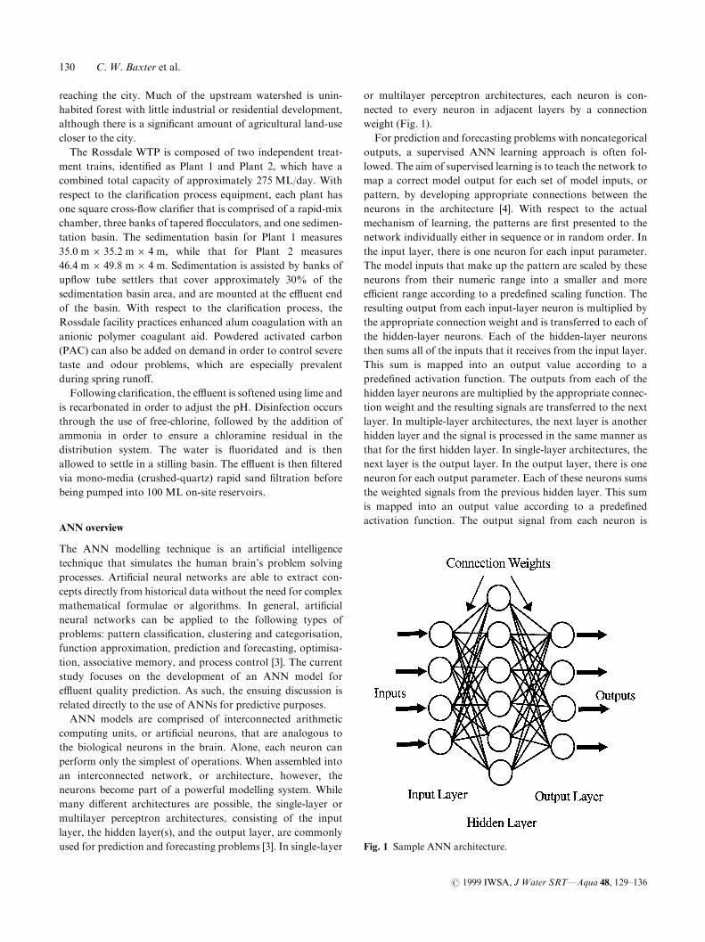
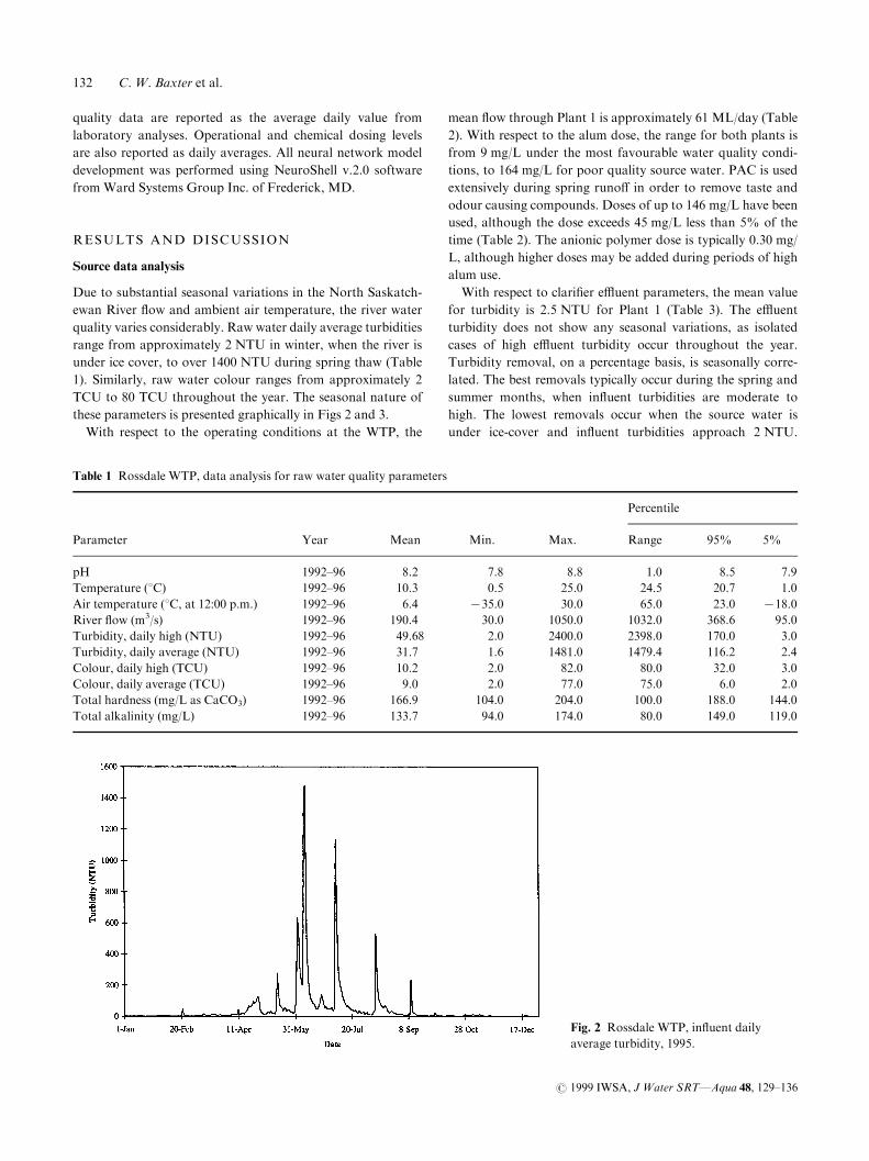
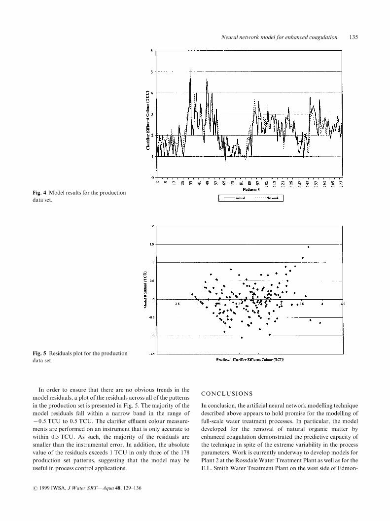
J Water SRTÐ Aqua Vol. 48, No. 4, pp. 129±136, 1999

Development of a full-scale arti®cial neural network model for the

removal of natural organic matter by enhanced coagulation

C. W. Baxter, S. J. Stanley and Q. Zhang, Environmental Engineering and Science Program, Department of Civil and Environmental

Engineering, University of Alberta, Room 304, Environmental Engineering Building, Edmonton, AB, T6G 2M8, Canada

ABSTRACT: Described is the development of a full-scale arti®cial neural network (ANN) model for the

removal of natural organic matter (NOM) by enhanced coagulation at the Rossdale Water Treatment Plant

(WTP) in Edmonton, Alberta, Canada. Few attempts have been made to develop a full-scale model of the

enhanced coagulation process due to extreme variability in the process parameters and the complex

nonlinear relationships between them. When applied to previously unseen data, the model predicted e�uent

colour with a high degree of accuracy. The model will be incorporated into real-time process control at the

WTP following a period of online testing.

INTRODUCTION

As water treatment regulations for the removal of organic,

biological, and other contaminants become more stringent,

water utilities must actively seek out new technologies that

improve treatment process control. In the water treatment

industry, each process is governed by complex nonlinear

relationships between numerous physical, chemical, and opera-

tional parameters. Historically, attempts have been made to

model these relationships by ®tting bench-scale data to mathe-

matical formulae. Such attempts have generally been unable to

account for the simultaneous change in more than one or two

of the key process parameters, and often fail when applied to

full-scale systems. As a result, current process control in the

water treatment industry is not model-based, but rather relies

upon a set of loosely de®ned heuristics in combination with the

expert-knowledge of the plant operators.

In order to improve treatment processes, plant operators

need tools that will allow them to select appropriate opera-

tional conditions required to achieve a desired e�uent quality

based on instantaneous in¯uent water quality. One such tool is

the arti®cial neural network (ANN), a robust arti®cial intelli-

gence modelling technique which has the ability to learn trends

and patterns in historical data in order to correctly classify new

data. With respect to water treatment processes, the ANN

modelling approach can be used to map the relationship

between in¯uent and e�uent parameters, resulting in a process

model that is based on full-scale operational data.

The purpose of this study is to illustrate the application of

arti®cial neural networks to water treatment processes through

the development of ANN model for natural organic matter

(NOM) removal by enhanced coagulation at a large water

treatment plant (WTP).

NOM and enhanced coagulation

In conventional water treatment where chlorinated disinfec-

tants are used, disinfection by-products (DBPs), such as triha-

lomethanes (THMs) and haloacetic acids (HAAs) can form by

the reaction of residual chlorine with natural organic matter

(NOM) in the treated water. As many DBPs are suspected to be

carcinogenic, it is generally desirable to remove them from the

drinking water stream. For conventional treatment facilities,

removal is often best accomplished by enhanced coagulation

[1]. The process involves the use of additional coagulant in

clari®cation in order to improve the removal of disinfection by-

product (DPB) precursors, namely natural organic matter [2].

With respect to current clari®cation process control, chemi-

cal dosing levels are adjusted on the basis of the results of jar-

tests that are often performed infrequently throughout the

plant operator's shift and often after clari®ed water quality

begins to degrade. This methodology is reactive rather than

proactive; dosing levels generally can not be adjusted until an

upset occurs. As such, the magnitude of the upset is often

magni®ed due to the time lag between the change in in¯uent

water quality and the chemical dosing adjustments. In addition

the requirement to now determine the optimal dose for both

particulate and organic removal adds signi®cant complexity to

jar testing methodologies. The optimal dosing levels deter-

mined by the bench-scale jar tests may also di�er from those in

full-scale operations due to the di�erences in the hydrody-

namics of the two systems. In spite of these problems, the jar-

test is widely used for determining dosing levels because there

are no suitable full-scale models of the clari®cation process.

Rossdale Water Treatment Plant description

The Rossdale Water Treatment Plant (WTP), owned and

operated by AQUALTA, is located on the North Saskatche-

wan River, a major tributary in the Saskatchewan-Nelson river

system, within the boundaries of the City of Edmonton. The

river has its headwaters in the Canadian Rocky Mountains and

¯ows in an easterly direction for approximately 500 km before

# 1999 IWSA 129

reaching the city. Much of the upstream watershed is unin-

habited forest with little industrial or residential development,

although there is a signi®cant amount of agricultural land-use

closer to the city.

The Rossdale WTP is composed of two independent treat-

ment trains, identi®ed as Plant 1 and Plant 2, which have a

combined total capacity of approximately 275 ML/day. With

respect to the clari®cation process equipment, each plant has

one square cross-¯ow clari®er that is comprised of a rapid-mix

chamber, three banks of tapered ¯occulators, and one sedimen-

tation basin. The sedimentation basin for Plant 1 measures

35.0 m6 35.2 m6 4 m, while that for Plant 2 measures

46.4 m6 49.8 m6 4 m. Sedimentation is assisted by banks of

up¯ow tube settlers that cover approximately 30% of the

sedimentation basin area, and are mounted at the e�uent end

of the basin. With respect to the clari®cation process, the

Rossdale facility practices enhanced alum coagulation with an

anionic polymer coagulant aid. Powdered activated carbon

(PAC) can also be added on demand in order to control severe

taste and odour problems, which are especially prevalent

during spring runo�.

Following clari®cation, the e�uent is softened using lime and

is recarbonated in order to adjust the pH. Disinfection occurs

through the use of free-chlorine, followed by the addition of

ammonia in order to ensure a chloramine residual in the

distribution system. The water is ¯uoridated and is then

allowed to settle in a stilling basin. The e�uent is then ®ltered

via mono-media (crushed-quartz) rapid sand ®ltration before

being pumped into 100 ML on-site reservoirs.

ANN overview

The ANN modelling technique is an arti®cial intelligence

technique that simulates the human brain's problem solving

processes. Arti®cial neural networks are able to extract con-

cepts directly from historical data without the need for complex

mathematical formulae or algorithms. In general, arti®cial

neural networks can be applied to the following types of

problems: pattern classi®cation, clustering and categorisation,

function approximation, prediction and forecasting, optimisa-

tion, associative memory, and process control [3]. The current

study focuses on the development of an ANN model for

e�uent quality prediction. As such, the ensuing discussion is

related directly to the use of ANNs for predictive purposes.

ANN models are comprised of interconnected arithmetic

computing units, or arti®cial neurons, that are analogous to

the biological neurons in the brain. Alone, each neuron can

perform only the simplest of operations. When assembled into

an interconnected network, or architecture, however, the

neurons become part of a powerful modelling system. While

many di�erent architectures are possible, the single-layer or

multilayer perceptron architectures, consisting of the input

layer, the hidden layer(s), and the output layer, are commonly

used for prediction and forecasting problems [3]. In single-layer

or multilayer perceptron architectures, each neuron is con-

nected to every neuron in adjacent layers by a connection

weight (Fig. 1).

For prediction and forecasting problems with noncategorical

outputs, a supervised ANN learning approach is often fol-

lowed. The aim of supervised learning is to teach the network to

map a correct model output for each set of model inputs, or

pattern, by developing appropriate connections between the

neurons in the architecture [4]. With respect to the actual

mechanism of learning, the patterns are ®rst presented to the

network individually either in sequence or in random order. In

the input layer, there is one neuron for each input parameter.

The model inputs that make up the pattern are scaled by these

neurons from their numeric range into a smaller and more

e�cient range according to a prede®ned scaling function. The

resulting output from each input-layer neuron is multiplied by

the appropriate connection weight and is transferred to each of

the hidden-layer neurons. Each of the hidden-layer neurons

then sums all of the inputs that it receives from the input layer.

This sum is mapped into an output value according to a

prede®ned activation function. The outputs from each of the

hidden layer neurons are multiplied by the appropriate connec-

tion weight and the resulting signals are transferred to the next

layer. In multiple-layer architectures, the next layer is another

hidden layer and the signal is processed in the same manner as

that for the ®rst hidden layer. In single-layer architectures, the

next layer is the output layer. In the output layer, there is one

neuron for each output parameter. Each of these neurons sums

the weighted signals from the previous hidden layer. This sum

is mapped into an output value according to a prede®ned

activation function. The output signal from each neuron is

Fig. 1 Sample ANN architecture.

130 C. W. Baxter et al.

# 1999 IWSA, J Water SRTÐAqua 48, 129±136

then processed by the inverse of the scaling function used in

the input layer in order to obtain an output value in the

appropriate numeric range. This value, which is the model

predicted value, is compared to the correct value for the given

patterns and the connection weights are modi®ed to decrease

the sum of squared error according to a preselected learning

algorithm. The entire process is repeated until the ANN

produces a su�ciently small error on a previously unseen

data set [5].

MATERIALS AND METHODS

ANN model development

The arti®cial neural network modelling process involves three

distinct stages: source data analysis, preliminary model devel-

opment, and model optimisation.

The primary objectives of the source data analysis are to gain

a familiarity with the study domain and to examine the

applicability of available data for model development. Initially,

the problem domain must be thoroughly examined, since the

blind application of the ANN technique to problems that have

not been thoroughly studied will lead to the development of

models with poor generalisation capabilities. Following the

domain study, all the available pertinent data are examined

and subjected to comprehensive statistical analyses in order to

determine the range, seasonal and daily trends, and other

important data characteristics. Based on the results of the data

analysis, the size and range of the data set to be used in model

development are selected.

The objective of the preliminary model design stage is to

design and evaluate a series of network architectures that, when

optimised, can be used as an e�ective process model. This

objective is best met through the use of a four-step scheme

which includes the selection of input and output parameters,

the organisation of the data patterns, the selection of initial

factors and levels of analysis, and the evaluation of potential

architectures. With respect to the selection of input and output

parameters, the output parameter which best represents the

process is selected. In general, only one output parameter is

selected as single-output models are generally more accurate

than multiple-output models. Each input parameter is selected

based on data availability and the likelihood of there being a

cause-e�ect relationship between it and the output parameter.

Once the model parameters are selected, the data patterns are

selected to re¯ect the availability of the data. Incomplete

patterns, as well as those that appear to be inconsistent with

the remaining data, are removed.

The data are initially organised into two categories based on

the value of the output parameter. The boundary is selected

according to process performance criteria and separates regular

operating conditions from process upset or special case condi-

tions. In order to develop a successful model, the data must be

further divided into three fractions: the training set, the test set,

and the production set. The training set consists of data

patterns that the network processes repeatedly in order to

learn trends and patterns in the data. During the learning

process, the network is periodically evaluated using the test set

patterns in order to ensure that the network is not simply

memorising the training data. The trained network is applied to

the production set which consists of data that the network has

never `seen' before in order to asses the performance of the

model. Each of these data sets contains an equal percentage of

special case data in order to ensure that the model is trained,

tested, and evaluated over a similar range of e�uent quality.

In designing the initial architectures, many factors need to be

considered including the type of architecture, the number of

layers, the number of neurons in each layer, the type of scaling

and activation functions, and the learning approach. In order

to determine the optimal levels of each of these factors, the

factorial experimental design approach is applied. This statis-

tical method is used for studying the e�ects of varying the levels

of multiple parameters in a limited number of runs. For an in-

depth discussion on the mechanisms of factorial-design experi-

mentation, please refer to the text by Box & Hunter [6].

In order to assess the model's performance, two separate

statistical indicators are applied to the production data set. The

R2 value compares the accuracy of the model to the accuracy of

a trivial benchmark model wherein the prediction is just the

mean of all the samples. A perfect ®t would result in anR2 value

of 1, a very good ®t near 1, and a very poor ®t near 0. The R2

indicator is applied to the entire production data set and

therefore serves as a measure of the model's performance in

periods of routine operation as well as during special-case

scenarios. The second statistical indicator, the average absolute

error, is used to compare the actual process outputs with the

network predictions. This indicator can serve to highlight

inconsistencies in model predictions and can also be used to

determine whether the model predictions are adequate for

process control.

In the model optimisation stage, the most promising candi-

date models are optimised through the ®ne-tuning of the

network architectures in order to minimise the error on the

production set data. The optimal model will be able to follow

daily trends in plant operations in addition to predicting the

special case patterns. In addition the model should produce

consistent results for all three data sets. The model should also

be insensitive to retraining following a swapping of the testing

and production sets. Finally, a plot of the model residuals

should be free of obvious trends.

Data handling and software

Three years of daily water quality and operational data, from

1994 to 1996, were used in the development of the ANN model

for the Rossdale WTP. The model described here is for Plant 1.

All data was obtained from AQUALTA, the water utility that

oversees the operation of the Rossdale facility. In¯uent water

Neural network model for enhanced coagulation 131

# 1999 IWSA, J Water SRTÐAqua 48, 129±136

quality data are reported as the average daily value from

laboratory analyses. Operational and chemical dosing levels

are also reported as daily averages. All neural network model

development was performed using NeuroShell v.2.0 software

from Ward Systems Group Inc. of Frederick, MD.

RESULTS AND DISCUSSION

Source data analysis

Due to substantial seasonal variations in the North Saskatch-

ewan River ¯ow and ambient air temperature, the river water

quality varies considerably. Raw water daily average turbidities

range from approximately 2 NTU in winter, when the river is

under ice cover, to over 1400 NTU during spring thaw (Table

1). Similarly, raw water colour ranges from approximately 2

TCU to 80 TCU throughout the year. The seasonal nature of

these parameters is presented graphically in Figs 2 and 3.

With respect to the operating conditions at the WTP, the

mean ¯ow through Plant 1 is approximately 61 ML/day (Table

2). With respect to the alum dose, the range for both plants is

from 9 mg/L under the most favourable water quality condi-

tions, to 164 mg/L for poor quality source water. PAC is used

extensively during spring runo� in order to remove taste and

odour causing compounds. Doses of up to 146 mg/L have been

used, although the dose exceeds 45 mg/L less than 5% of the

time (Table 2). The anionic polymer dose is typically 0.30 mg/

L, although higher doses may be added during periods of high

alum use.

With respect to clari®er e�uent parameters, the mean value

for turbidity is 2.5 NTU for Plant 1 (Table 3). The e�uent

turbidity does not show any seasonal variations, as isolated

cases of high e�uent turbidity occur throughout the year.

Turbidity removal, on a percentage basis, is seasonally corre-

lated. The best removals typically occur during the spring and

summer months, when in¯uent turbidities are moderate to

high. The lowest removals occur when the source water is

under ice-cover and in¯uent turbidities approach 2 NTU.

Table 1 Rossdale WTP, data analysis for raw water quality parameters

Percentile

Parameter Year Mean Min. Max. Range 95% 5%

pH 1992±96 8.2 7.8 8.8 1.0 8.5 7.9

Temperature (8C) 1992±96 10.3 0.5 25.0 24.5 20.7 1.0

Air temperature (8C, at 12:00 p.m.) 1992±96 6.4 735.0 30.0 65.0 23.0 718.0

River ¯ow (m3/s) 1992±96 190.4 30.0 1050.0 1032.0 368.6 95.0

Turbidity, daily high (NTU) 1992±96 49.68 2.0 2400.0 2398.0 170.0 3.0

Turbidity, daily average (NTU) 1992±96 31.7 1.6 1481.0 1479.4 116.2 2.4

Colour, daily high (TCU) 1992±96 10.2 2.0 82.0 80.0 32.0 3.0

Colour, daily average (TCU) 1992±96 9.0 2.0 77.0 75.0 6.0 2.0

Total hardness (mg/L as CaCO3) 1992±96 166.9 104.0 204.0 100.0 188.0 144.0

Total alkalinity (mg/L) 1992±96 133.7 94.0 174.0 80.0 149.0 119.0

Fig. 2 Rossdale WTP, in¯uent daily

average turbidity, 1995.

132 C. W. Baxter et al.

# 1999 IWSA, J Water SRTÐAqua 48, 129±136

Under such conditions, it is sometimes possible for turbidity to

increase through the treatment processes, resulting in negative

removals of turbidity. Similar trends are observed for e�uent

colour and colour removal, although negative removals of

colour are seldom observed.

Preliminary model development

In order to select appropriate input and output parameters for

the model, the study domain must be thoroughly examined.

From recent literature in the areas of disinfection by-products

and enhanced coagulation, over 30 potential model input

parameters, as well as a number of potential outputs were

identi®ed. From these, 12 parameters were selected and

grouped according to their source (Table 4). The water quality

parameters provide a general indication of the quality of the

WTP source water. The operational parameters are those that

can be readily controlled by the plant operator and include

chemical dosing levels as well as the over¯ow rate through the

clari®ers. The lag-1 time series parameters are included as both

in¯uent turbidity and in¯uent colour are correlated over time.

With respect to the output parameter, total organic carbon

(TOC), ultraviolet absorbance at a wavelength of 254 nm

(UVA-254), trihalomethane formation potential (THMFP),

and colour are the most common surrogate parameters used to

measure NOM. From these parameters, clari®er e�uent colour

was selected as the model output due to the availability and

reliability of colour data at the Rossdale WTP.

The entire data set consists of 889 separate days or patterns,

spanning three years of water treatment at the Rossdale Water

Fig. 3 Rossdale WTP, in¯uent daily

average colour, 1995.

Table 2 Rossdale WTP, data analysis for

process parameters Percentile

Parameter Dates Mean Min. Max. Range 95% 5%

Raw ¯ow, Plant 1 (ML/day) 1992±96 61.2 0.0 125.0 125.0 97.6 0.0

Alum dose, Plant 1 (mg/L) 1992±96 31.8 9.0 164.0 155.0 71.1 15.0

PAC dose, Plant 1 (mg/L) 1992±96 10.7 0.0 145.6 145.6 46.0 0.0

Polymer dose, Plant 1 (mg/L) 1992±96 0.29 0.00 0.87 0.87 0.51 0.00

Table 3 Rossdale WTP, data analysis for

clari®er e�uent parameters Percentile

Parameter Dates Mean Min. Max. Range 95% 5%

E�uent turbidity, Plant 1 (NTU) 1992±96 2.5 0.4 11.6 11.2 4.8 1.0

Turbidity removal, Plant 1 (%) 1992±96 61.6 7129.4 99.9 229.3 98.4 73.5

E�uent colour, Plant 1 (TCU) 1992±96 2.1 0.5 7.4 6.9 3.8 1.0

Colour removal, Plant 1 (%) 1992±96 61.7 7221.9 98.7 320.6 92.0 25.0

Neural network model for enhanced coagulation 133

# 1999 IWSA, J Water SRTÐAqua 48, 129±136

Treatment Plant. The data are initially organised into two

categories based on the value of the output parameter. The

boundary separating the data corresponds to the 90th percen-

tile of the clari®er e�uent colour and has a numerical value of

3.20 TCU. Operationally, this value is also signi®cant as it

approximates the boundary between acceptable and poor

clari®er e�uent colour at the Rossdale WTP. Data for which

the clari®er e�uent colour exceeds 3.2 TCU falls into the

special-case scenario category, while the remaining data corre-

sponds to normal operating conditions at the WTP. The data

was further divided into the training, testing, and production

sets according to the method previously outlined.

For the preliminary model development stage, the e�ects of

some of the most signi®cant factors were evaluated using

factorial design experimentation. A sample design, including

factors and their corresponding initial levels of analysis, is

presented in Table 5. Both the factors and the initial levels of

analysis were selected based on previous experience in ANN

modelling.

Model optimisation

From the preliminary model design stage, a number of poten-

tial candidate model architectures were selected for further

optimisation. Of these, the three-layer backpropagation archi-

tecture, a standard ANN architecture in which information is

processed forward through the network and the prediction

error is propagated backwards through the network, produced

the most favourable results. When the trained network was

applied to each of the data sets, the results were consistent,

ranging from an R2 of 0.71 for the testing set to 0.76 for the

training set (Table 6). Similarly, the mean absolute error ranged

from 0.30 TCU for the training set to 0.32 TCU for the testing

set. In addition, when the testing and production data sets were

swapped and the model was retrained and applied to the new

production set, the results are identical to those for the original

test set. This suggests that the internal network structure is

identical for both the original and swapped data, since the

original test set contains the same data patterns as the new

production set. As such, the model architecture is decidedly

stable, a requirement for use in process control.

The model results for previously unseen data (production

data) are presented graphically in Fig. 4. The model follows

the trends in the actual clari®er e�uent data quite well,

although two areas of apparent inaccuracy require a further

examination. In the ®rst 15 patterns, when the actual clari®er

e�uent colour ranges from approximately 1±2 TCU, the

network tends to over-predict the actual values. From a

process control standpoint however, this error is negligible

since these patterns correspond to late-winter days where the

raw water quality conditions are ideal and process control

modi®cations are rarely required. With respect to the second

area of concern, the model has some di�culty in predicting

the highest clari®er e�uent colour peaks. While the model

clearly recognised that there is a peak, it tends to under-

predict the actual e�uent colour by approximately 1 TCU.

The actual e�uent colour peaks are the result of mild upsets

in the clari®cation process, as they do not fall within the range

of regular operating conditions. Since the goal of the model-

ling process is to develop a model that can be used in process

control to avoid such upsets, it is not absolutely necessary for

the model to be able to predict these peaks with complete

accuracy. It is far more important that the model has good

predictive capacity in the normal operating range (53 TCU)

of clari®er e�uent colour. In this range, the model accuracy

increases, with an average absolute error of only 0.28 TCU on

the production set.

Table 4 Model input parameters

Input parameter Parameter classi®cation

In¯uent turbidity Water quality

In¯uent colour Water quality

In¯uent pH Water quality

In¯uent water temperature Water quality

In¯uent alkalinity Water quality

In¯uent hardness Water quality

Alum dose Operational

PAC dose Operational

Polymer dose Operational

Over¯ow rate Operational

Lag 1 turbidity Time series

Lag 1 colour Time series

Table 5 Sample factorial design, 3-layer backpropagation

architecture

Factor 7 level + level

Ratio of training to testing data 1:1 2:1

Total number of hidden layer neurons 30 120

Activation function Logistic Gaussian

Compliment

Table 6 Model results

Mean absolute error

Data set R2 (TCU)

Training 0.76 0.30

Testing 0.71 0.32

Production 0.75 0.31

Production (cross-test) 0.71 0.32

134 C. W. Baxter et al.

# 1999 IWSA, J Water SRTÐAqua 48, 129±136

In order to ensure that there are no obvious trends in the

model residuals, a plot of the residuals across all of the patterns

in the production set is presented in Fig. 5. The majority of the

model residuals fall within a narrow band in the range of

70.5 TCU to 0.5 TCU. The clari®er e�uent colour measure-

ments are performed on an instrument that is only accurate to

within 0.5 TCU. As such, the majority of the residuals are

smaller than the instrumental error. In addition, the absolute

value of the residuals exceeds 1 TCU in only three of the 178

production set patterns, suggesting that the model may be

useful in process control applications.

CONCLUSIONS

In conclusion, the arti®cial neural network modelling technique

described above appears to hold promise for the modelling of

full-scale water treatment processes. In particular, the model

developed for the removal of natural organic matter by

enhanced coagulation demonstrated the predictive capacity of

the technique in spite of the extreme variability in the process

parameters. Work is currently underway to develop models for

Plant 2 at the RossdaleWater Treatment Plant as well as for the

E.L. Smith Water Treatment Plant on the west side of Edmon-

Fig. 4 Model results for the production

data set.

Fig. 5 Residuals plot for the production

data set.

Neural network model for enhanced coagulation 135

# 1999 IWSA, J Water SRTÐAqua 48, 129±136

ton. Following a period of on-line testing and revision, these

models will be incorporated into clari®cation process control in

order to minimise upsets in the clari®cation process.

ACKNOWLEDGEMENTS

We are indebted to both the American Water Works Research

Foundation (AWWARF) and AQUALTA for their ®nancial

support and partnership throughout the research. In particular,

Simon Thomas and Riyaz Shari�, both of AQUALTA, were

instrumental in providing the data and operations information

required for the model development.

BIBLIOGRAPHY

1 Krasner SW, Amy G. Jar-test evaluations of enhanced coagula-

tion. JAWWA 1995; 87(10): 93±107.

2 Crozes G,White P, Marshall M. Enhanced coagulation: its e�ect

on NOM removal and chemical costs. JAWWA 1995; 87(1): 78±

89.

3 Jain AK, Mao J. Arti®cial neural networks: a tutorial. Computer

1996; 29(3): 31±44.

4 Daniell TM. Neural networksÐapplications in hydrology and

water resources engineering. In: Barton AC, ed. Proceedings of

the International Hydrology and Water Resources Symposium. 2±

4 October 1991, Perth, Australia, Institute of Engineers of

Australia, 1991: 797±802.

5 Boger Z. Applications of neural networks to water and waste-

water treatment plant operation. ISA Transactions 1992; 31(1):

25±31.

6 Box GEP, HunterWJ, Hunter JS. Factorial designs at two levels.

In: Bradley RA, Hunter JS, eds. Statistics for Experimenters, pp.

306±342. New York, NY: John Wiley & Sons, 1978.

136 C. W. Baxter et al.

# 1999 IWSA, J Water SRTÐAqua 48, 129±136