Page 1
1
Certification of Thesis
Development of a magnetically
levitated axial field brushless DC
motor
by
Markus Raab
Submitted to the Department of
Mechatronics
In partial fulfilment of the requirement for the degree of
Master of Engineering (M.Eng.)
at
Aalen University
of Applied Sciences
Supervising Professors:
Prof. Kazi (Aalen University)
Prof. Trumper (MIT)
Page 2
2
Certification of Thesis
Page 3
3
Certification of Thesis
Certification of Thesis
I certify that the ideas, experimental work, results, analyses, software and conclusions re-
ported in this thesis are entirely my effort, except where otherwise acknowledged. I also
certify that the work is original and has not been previously submitted for any other award,
expect where otherwise acknowledged.
________________________ _________________________
Date Signature of Candidate
Page 4
4
Acknowledgments
Acknowledgments
I would sincerely like to thank and acknowledge the following people for their assistance,
guidance and support throughout the duration of this thesis project.
First of all I would like to thank my supervisors Prof. Kazi from Aalen University and Prof.
Trumper from MIT. Both helped me a lot during the work of this thesis.
Prof. Trumper offered me to stay in his Precision Motion Control lab at MIT as a visiting stu-
dent for one semester. During my stay I learned a lot about the design and control of mecha-
tronic systems. Especially in the 2.737 mechatronics course where I could help as a teaching
assistant I could improve my knowledge about the interaction of mechanical, electrical and
control systems. In many discussions Prof. Trumper supported my work with a lot of good
ideas about the conception and control of the motor design and encouraged me to work
eagerly on my project. Thank you very much for the opportunity to stay in your lab and your
help.
I also want to thank Prof. Kazi who supervised the second part of my thesis. In all meetings
he improved my design with good ideas and helped me to get the whole concept working. I
also want to thank him, for the support in different other student project during my studies.
Thanks a lot to Laura Zaganjori who helped me organizing my stay at MIT and was always
there to make things working.
I am also grateful to all of my labmates from the Precision Motion Control Lab of MIT and
the Actuator and Sensors Lab of the University Aalen for the support, interest and assistance
in this thesis project. Especially I want to thank Alex Adrien who was with me at MIT as a
visiting student. Together we could tackle all the difficulties when we arrived in Cambridge. I
had good discussions during my work with him. I also want to thank Lei Zhou and Jun Young
Yoon which have helped me a lot with different questions regarding technical questions and
my stay in the Lab. Also I want to thank Minkyun Noh, Phillip Daniel and Maria Pina Piccolo
which worked with me in the Precision Motion Control Lab. Back in Germany, Klaus Winter-
mayr worked with me in the Actuator and Sensors Lab where we had good dialogues about
different technical questions.
I want to thank the German National Academic Foundation who supported me during my
studies and my stay in the USA.
Finally I want to thank my fiancée and family which supported me during my whole studies.
Page 5
5
Abstract
Abstract
Brushless DC (BLDC) motors are often used in industrial applications because of their robust-
ness and their low maintenance. On the other hand reluctance actuators are also used in a
wide range of industry starting with simple binary actuators up to high precision applica-
tions. For this reason it is important to teach students about the design, calculation and con-
trol of these devices.
In this thesis, a modular brushless DC motor with a reluctance based magnetically levitated
rotor is developed, as a teaching tool for universities. Because of its simple design, it is pos-
sible to build this system using standard manufacturing techniques available in most work-
shops. The low costs approach of the setup features the National Instrument myRIO board.
The modular concept allows the use of the system in different levels of teaching. In its basic
configuration, the commutation of BLDC motors as well as the design of position controllers
by using model based design can be demonstrated. The next step focuses on the teaching of
the magnetically levitation of a disc, in this step forces of reluctance actuators , couplings
between different axes and the control of nonlinear system can be explained. In the final
step, the motor can be run magnetically levitated and in six degrees of freedom controlled.
In this thesis all the necessary files and algorithms are presented, which are to needed build
and run the system.
Page 6
6
Kurzfassung
Kurzfassung
Bürstenlose Gleichstrommotoren erfreuen sich aufgrund ihrer Robustheit sowie ihres war-
tungsarmen Betriebes zunehmender Beliebtheit in industriellen Anwendungen. Ein weiteres
weit verbreitetes Aktuator Prinzip sind Reluktanzaktuatoren, welche binär angesteuerten für
einfache Schaltanwendungen bis hin zum Hochpräzisenbereich Anwendung finden. Aus die-
sem Grund ist es wichtig, Fachleute in der Auslegung, Berechnung sowie der Regelung dieser
Geräte auszubilden.
Im Rahmen dieser Arbeit wird ein modular aufgebauter mit Reluktanzaktuatoren magnetisch
gelagerter bürstenloser Gleichstrommotor (BLDC) entwickelt, welcher in der Lehre an Uni-
versitäten und Hochschulen eingesetzt werden kann. Durch einen einfachen Aufbau ist es
möglich, das System mit standartmäßigen Herstellungsverfahren und geringen Kosten zu
fertigen. Als Echtzeit System wird das von National Instruments vertriebene System NI-
myRIO verwendet.
Durch den modularen Aufbau ist es möglich, das System in verschiedenen Ausbildungsstufen
einzusetzen. In der Grundstufe kann die Kommutierung von BLDC Motoren, sowie das Erstel-
len von Positionsregelungen auf Basis der modellbasierten Funktionsentwicklung gelehrt
werden. In der nächsten Stufe wird eine Stahlscheibe magnetisch gelagert. Hierbei können
die Kräfte und das Verhalten von Reluktanzaktuatoren erklärt werden, des Weiteren kann
die Entkopplung und Regelung von nichtlinearen Systemen vermittelt werden. In der finalen
Stufe wird der Motor in sechs Freiheitsgraden magnetisch gelagert betrieben.
Diese Arbeit umfasst alle benötigten Dokumente und Algorithmen die für den Bau und Be-
trieb des Systems benötigt werden.
Page 7
7
Contents
Contents
Certification of Thesis ................................................................................................................. 3
Acknowledgments ...................................................................................................................... 4
Abstract ...................................................................................................................................... 5
Kurzfassung ................................................................................................................................. 6
Contents ..................................................................................................................................... 7
List of Figures ............................................................................................................................ 11
List of Tables ............................................................................................................................. 15
1 Introduction ...................................................................................................................... 16
2 Conceptual design ............................................................................................................ 18
2.1 Overview brushless DC motors .................................................................................. 18
2.1.1 Basics of DC motors ............................................................................................ 18
2.1.2 Commutation ...................................................................................................... 18
2.1.3 Types of brushless DC motors ............................................................................ 20
2.2 Overview magnetic bearings ..................................................................................... 21
2.2.1 Reluctance actuators in magnetic levitation ...................................................... 21
2.2.2 Magnetic bearings .............................................................................................. 22
2.3 Actuation concept ...................................................................................................... 23
2.3.1 Vertical actuation ............................................................................................... 23
2.3.2 Horizontal actuation ........................................................................................... 24
2.4 Sensor concept ........................................................................................................... 26
2.4.1 Sensing of the motor angle ................................................................................ 26
2.4.2 Position sensing for magnetic bearings .............................................................. 27
2.5 Rotor concept ............................................................................................................ 28
2.6 Concept for a Maglev BLDC motor ............................................................................ 29
2.6.1 BLDC motor ......................................................................................................... 29
2.6.2 Magnetic levitation ............................................................................................. 30
2.6.3 Magnetically levitated BLDC motor .................................................................... 31
3 Axial field brushless DC motor.......................................................................................... 32
3.1 Coil design .................................................................................................................. 32
Page 8
8
Contents
3.1.1 Winding structure ............................................................................................... 32
3.1.2 Coil Design .......................................................................................................... 36
3.2 Rotor design ............................................................................................................... 38
3.2.1 Magnetic material .............................................................................................. 38
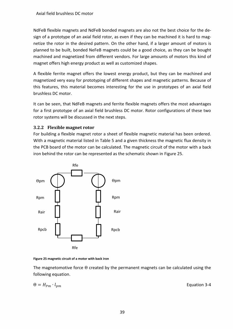
3.2.2 Flexible magnet rotor ......................................................................................... 39
3.2.3 NeFdB magnet rotor ........................................................................................... 42
3.2.4 Comparison of the rotor configurations............................................................. 43
3.3 Position sensor ........................................................................................................... 44
3.4 Parameter calculation ................................................................................................ 46
3.4.1 Torque constant ................................................................................................. 46
3.4.2 Back EMF ............................................................................................................ 48
3.4.3 Coil Resistance .................................................................................................... 49
3.4.4 Coil current calculation ....................................................................................... 50
3.4.5 Coil Inductance ................................................................................................... 50
3.4.6 Moment of inertia .............................................................................................. 51
3.4.7 Summary of the motor Parameters ................................................................... 51
3.5 Motor design .............................................................................................................. 51
3.5.1 Bearing design .................................................................................................... 51
3.5.2 Electronics design ............................................................................................... 52
3.5.3 LabVIEW implementation ................................................................................... 54
3.5.4 Design summary ................................................................................................. 54
3.6 Motor parameter measurement ............................................................................... 56
3.6.1 Sine/cosine encoder reading test ....................................................................... 56
3.6.2 Coil characterization ........................................................................................... 60
3.6.3 Back EMF measurement ..................................................................................... 62
3.6.4 Damping estimation ........................................................................................... 64
3.7 Modelling and control of a brushless DC motor ........................................................ 67
3.7.1 Commutation ...................................................................................................... 67
3.7.2 Motor characteristics ......................................................................................... 68
3.7.3 Linearized model ................................................................................................ 70
3.7.4 Controller design ................................................................................................ 71
3.7.5 Trajectory based positioning .............................................................................. 72
Page 9
9
Contents
3.8 Model and control verification .................................................................................. 76
3.8.1 Open loop speed step ......................................................................................... 76
3.8.2 System frequency response measurement ........................................................ 76
3.8.3 Return ratio measurement ................................................................................. 77
3.8.4 Step response closed loop .................................................................................. 79
3.8.5 Trajectory based step response closed loop ...................................................... 79
4 Three axis magnetic bearing............................................................................................. 81
4.1 Magnetic bearing design ............................................................................................ 81
4.2 Position sensing ......................................................................................................... 82
4.2.1 Sensor selection .................................................................................................. 82
4.2.2 Sensor electronics ............................................................................................... 83
4.2.3 Sensor calibration ............................................................................................... 84
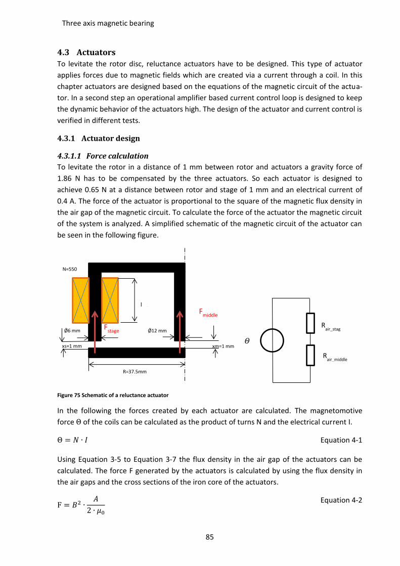
4.3 Actuators .................................................................................................................... 85
4.3.1 Actuator design .................................................................................................. 85
4.3.2 Actuator test ....................................................................................................... 89
4.3.3 Electronics design ............................................................................................... 90
4.4 Modelling and control................................................................................................ 95
4.4.1 System model ..................................................................................................... 95
4.4.2 Controller design ................................................................................................ 98
4.4.3 Controller tuning .............................................................................................. 107
4.4.4 Measurement of the system behavior for different axes ................................ 111
4.5 LabVIEW implementation ........................................................................................ 113
5 Magnetic bearing for two additional axes ..................................................................... 114
5.1 Detailed design horizontal axes bearing .................................................................. 114
5.2 Detailed rotor design for magnetic bearing ............................................................ 115
5.3 Actuators .................................................................................................................. 117
5.3.1 Actuator design ................................................................................................ 117
5.3.2 Actuator test ..................................................................................................... 119
5.3.3 Electronics design ............................................................................................. 120
5.4 Modelling and control.............................................................................................. 121
5.4.1 System model ................................................................................................... 121
5.4.2 Controller design .............................................................................................. 125
Page 10
10
Contents
5.4.3 Controller tuning .............................................................................................. 129
5.4.4 Measurement of the system behavior for different axes ................................ 130
6 BLDC motor with magnetic bearing ............................................................................... 132
6.1 System response of the magnetic bearing .............................................................. 132
6.2 Motor frequency response ...................................................................................... 134
6.3 Motor speed ............................................................................................................ 134
7 Conclusion and further work .......................................................................................... 136
8 Bibliography .................................................................................................................... 139
9 Appendix Motor.............................................................................................................. 144
9.1 Comparison of permanent magnet materials ......................................................... 144
9.2 Mechanical design ................................................................................................... 145
9.3 Test specifications .................................................................................................... 148
9.4 Matlab ...................................................................................................................... 157
9.4.1 Script for PCB coil printing ................................................................................ 157
9.4.2 Motormodell parameter script......................................................................... 164
10 Appendix magnetic bearing ............................................................................................ 165
10.1 Mechanical design ................................................................................................... 165
10.2 Test specifications .................................................................................................... 172
10.3 DSA Tool Test ........................................................................................................... 175
10.4 Simulink model ........................................................................................................ 176
Page 11
11
List of Figures
List of Figures
Figure 1 Schematic drawing of brushless and brushed DC motors .......................................... 18
Figure 2 brushed DC motor commutation taken from [3, p. 80] ............................................. 19
Figure 3 Bock commutation and Sine commutation ................................................................ 19
Figure 4 Radial field and axial field motors .............................................................................. 20
Figure 5 Disassembled floppy disc axial field motor ................................................................ 20
Figure 6 Schematic view of a reluctance actuator based magnetic levitation system ............ 21
Figure 7 Motor with magnetic bearings picture taken from [12, p. 3] .................................... 22
Figure 8 Actuator concept for Z, Pitch and Roll ........................................................................ 23
Figure 9 Actuation concept for the X and Y axis ....................................................................... 24
Figure 10 Optical quadrature encoder, picture taken from [13] ............................................. 26
Figure 11 Encoder signals of quadrature and sine/cosine encoders ....................................... 27
Figure 12 Sensor concept of the magnetic bearing.................................................................. 28
Figure 13 Rotor concept ........................................................................................................... 29
Figure 14 Motor with and without back iron ........................................................................... 29
Figure 15 Schematic drawing of the motor concept ................................................................ 30
Figure 16 Concept of the magnetic levitated brushless DC motor .......................................... 31
Figure 17 Overlapping winding structure ................................................................................. 33
Figure 18 Layers per Coil .......................................................................................................... 34
Figure 19 Through hole and not through hole connection ...................................................... 34
Figure 20 Schematic view of non-overlapping windings .......................................................... 35
Figure 21 Lorentz forces in a coil .............................................................................................. 36
Figure 22 Rhomboidal coil, coil with parallel active sections, picture taken from [17, p. 2] ... 36
Figure 23 Coil structure for different layers, picture taken from [17, p. 2] ............................. 37
Figure 24 Coils with straight lines and arc structure ................................................................ 38
Figure 25 magnetic circuit of a motor with back iron .............................................................. 39
Figure 26 CAD Magnetizing tool ............................................................................................... 40
Figure 27 magnetizing a flexible magnet rotor ........................................................................ 41
Figure 28 Self magnetized flexible magnet rotor ..................................................................... 41
Figure 29 CAD drawing of a NeFdB magnet ............................................................................. 42
Figure 30 Expected magnetic field in the coils ......................................................................... 42
Figure 31 2D Magnetic field simulation of the motor without back iron ................................ 43
Figure 32 NdFeB magnet placement tool and NdFeB rotor ..................................................... 43
Figure 33 Sine/cosine encoder reading .................................................................................... 44
Figure 34 Simulated min/max flux densities in the Hall sensors ............................................. 45
Figure 35 Description of the air gap flux density, picture taken from [19, p. 2] ..................... 47
Figure 36 Coil and area which is in magnetic field ................................................................... 48
Figure 37 Bearing bore ............................................................................................................. 52
Figure 38 Power electronics of the Motor ............................................................................... 53
Page 12
12
List of Figures
Figure 39 Sensor reading electronics ....................................................................................... 53
Figure 40 Designed BLDC motor with electronics and real time target ................................... 54
Figure 41 PCB Setup.................................................................................................................. 55
Figure 42 Designed PCB board ................................................................................................. 55
Figure 43 Comparison between measured and desired Hall sensor signal ............................. 56
Figure 44 Error between measured and simulated angle ........................................................ 57
Figure 45 Error curve of the measured angle and FFT analysis of the error signal ................. 57
Figure 46 Results of the fitted error fitting .............................................................................. 58
Figure 47 Measurement of the Angle error for different speed .............................................. 59
Figure 48 Measured and expected step response of the coil .................................................. 60
Figure 49 Measured and fitted step response of the coil ........................................................ 61
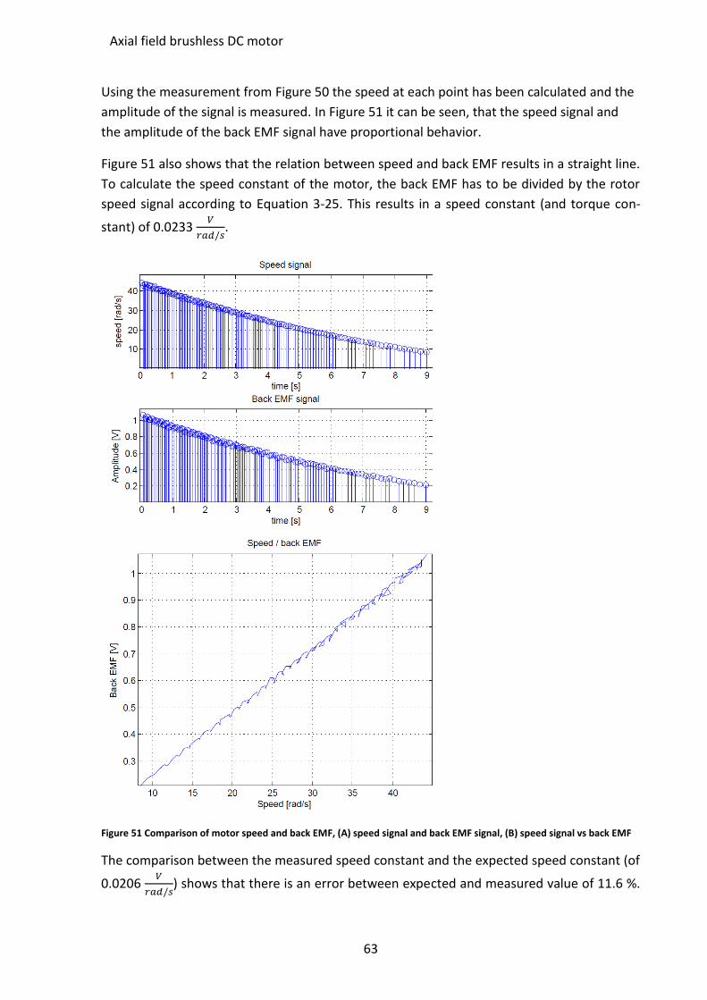
Figure 50 Back EMF signal ........................................................................................................ 62
Figure 51 Comparison of motor speed and back EMF, (A) speed signal and back EMF signal,
(B) speed signal vs back EMF .................................................................................................... 63
Figure 52 Back EMF shape ........................................................................................................ 64
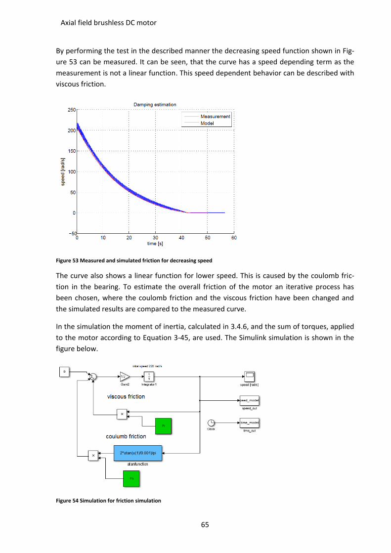
Figure 53 Measured and simulated friction for decreasing speed .......................................... 65
Figure 54 Simulation for friction simulation ............................................................................. 65
Figure 55 estimated Friction function ...................................................................................... 66
Figure 56 Top level of the BLDC motor model ......................................................................... 67
Figure 57 Simulink based BLDC commutation.......................................................................... 68
Figure 58 Simulink implementation of the voltage to torque behavoir of one coil ................ 69
Figure 59 Simulink implementation of the motor torque to speed/angle .............................. 70
Figure 60 Simulated frequency response of the motor ........................................................... 71
Figure 61 Controller structure .................................................................................................. 72
Figure 62 Simulated loop return ratio and controller bode plot ............................................. 72
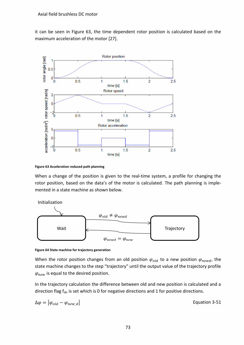
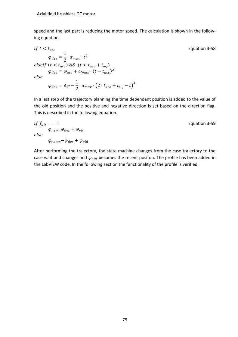
Figure 63 Acceleration reduced path planning ........................................................................ 73
Figure 64 State machine for trajectory generation .................................................................. 73
Figure 65 Comparison of measured on modeled open loop speed steps ............................... 76
Figure 66 Comparison between measured and simulated frequency response of the motor 77
Figure 67 Measured return ratio .............................................................................................. 78
Figure 68 Closed loop step response ........................................................................................ 79
Figure 69 Trajectory based positioning for 1 mrad and 1 rad .................................................. 79
Figure 70 Trajectory based positioning for one rotation and 10 rotations.............................. 80
Figure 71 Magnetic bearing for Z, Pitch and Roll axis .............................................................. 81
Figure 72 QTR-1A picture taken from [29] ............................................................................... 82
Figure 73 Sensing circuit ........................................................................................................... 83
Figure 74 Sensor calibration ..................................................................................................... 84
Figure 75 Schematic of a reluctance actuator .......................................................................... 85
Figure 76 Measured and fitted inductance of a coil ................................................................ 88
Figure 77 Actuator test, using electrical current vs. distance .................................................. 89
Figure 78 Current control schematic ........................................................................................ 90
Page 13
13
List of Figures
Figure 79 Bode plot U --> I coil ................................................................................................. 92
Figure 80 Bode plot current controller ..................................................................................... 93
Figure 81 Bode plot return ratio current control ..................................................................... 93
Figure 82 Measured and modeled step response of the current control ................................ 94
Figure 83 Model of the vertical axes ........................................................................................ 95
Figure 84 Placement of the reluctance actuators and sensors in the system ......................... 95
Figure 85 Distance caused by angle calculation ....................................................................... 97
Figure 86 System representation for linearization of the Z-axis .............................................. 99
Figure 88 Linearized system including current control .......................................................... 100
Figure 89 Linearized bode plot of the Z-axis .......................................................................... 101
Figure 90 System representation for linearization of the Pitch axis ...................................... 102
Figure 91 System representation for linearization of the Roll axis ........................................ 102
Figure 92 Linearized bode plot for rotary axis ....................................................................... 103
Figure 93 DSA system response measurement ...................................................................... 104
Figure 94 Z-Axis measured and calculated frequency response ............................................ 105
Figure 95 Pitch-Axis measured and calculated frequency response ...................................... 105
Figure 96 Roll-Axis measured and calculated frequency response ........................................ 106
Figure 97 Return Ratio Z-axis .................................................................................................. 107
Figure 98 DSA return ratio measurement .............................................................................. 108
Figure 99 Measured frequency response of the Z-axis .......................................................... 108
Figure 100 Return Ratio rotary axis ........................................................................................ 109
Figure 101 Measured frequency response of the Pitch axis .................................................. 110
Figure 102 Measured frequency response of the Roll axis .................................................... 110
Figure 103 Frequency response measurement for decoupling verification .......................... 111
Figure 104 Control efforts for changes in the Z axis .............................................................. 112
Figure 105 Control efforts for changes in the Pitch axis ........................................................ 112
Figure 106 Control efforts for changes in the Roll axis .......................................................... 113
Figure 107 Actuators and forces of a 5 DOF bearing ............................................................. 114
Figure 108 Detailed rotor design concepts ............................................................................ 115
Figure 109 Rotor design for low coupling .............................................................................. 115
Figure 110 Rotor with 3D printed ring for a constant surface ............................................... 116
Figure 111 Final motor and bearing design ............................................................................ 116
Figure 112 Figure of the final motor setup ............................................................................ 117
Figure 113 X, Y axis actuator .................................................................................................. 118
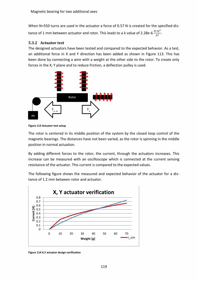
Figure 114 Actuator test setup ............................................................................................... 119
Figure 115 X,Y actuator design verification ............................................................................ 119
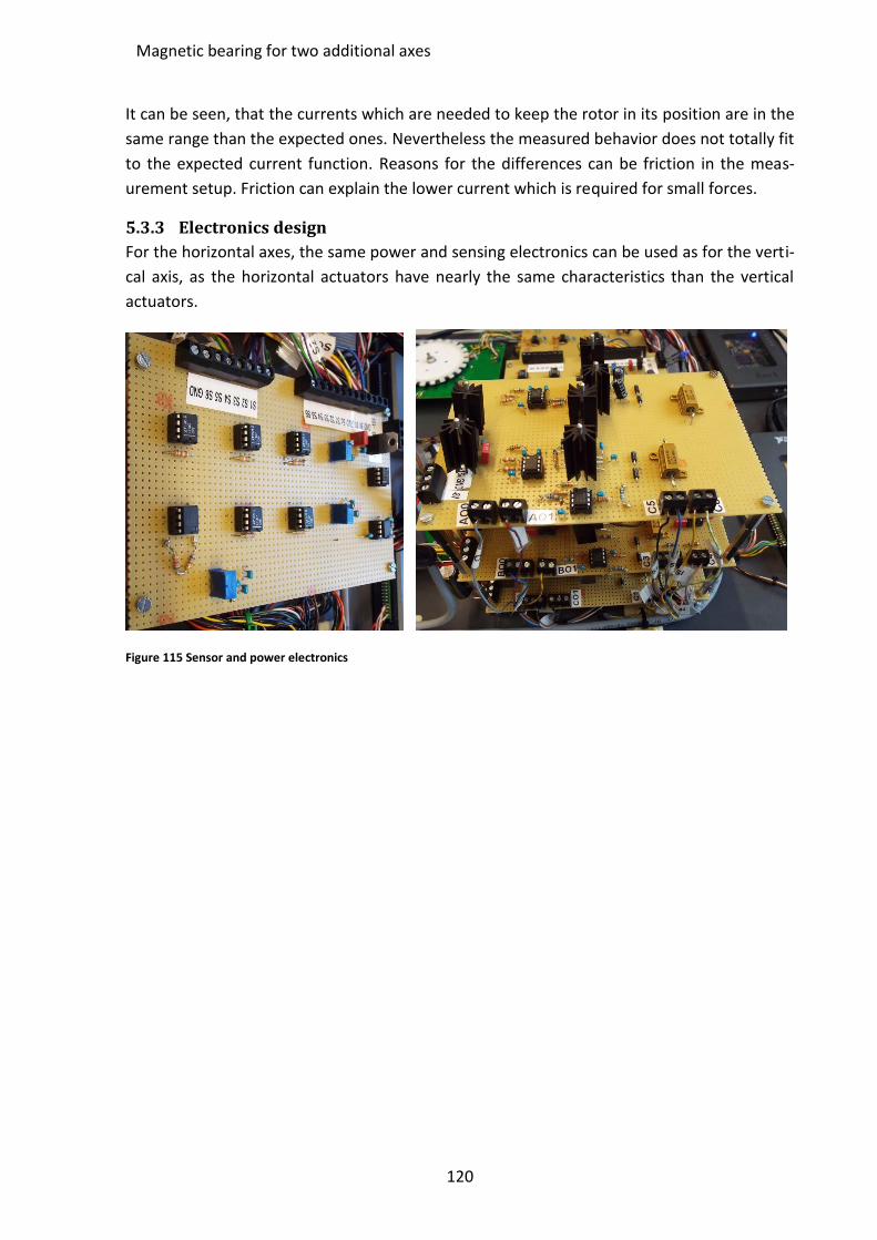
Figure 116 Sensor and power electronics .............................................................................. 120
Figure 117 Modeled of the horizontal axes ........................................................................... 121
Figure 118 Forces in X and Y axis ............................................................................................ 121
Figure 119 Sensor positions of the horizontal axes ............................................................... 122
Figure 120 Coupling between X, Y and Z, Roll, Pitch axis ....................................................... 124
Page 14
14
List of Figures
Figure 121 decoupling and trigonometric functions of the X axis ......................................... 126
Figure 122 Linearized bode plot of the X-axis ........................................................................ 127
Figure 123 X Axis measured and calculated frequency response .......................................... 128
Figure 124 Y Axis measured and calculated frequency response .......................................... 128
Figure 125 Measurement return ratio X axis ......................................................................... 129
Figure 126 Measurement return ratio Y axis ......................................................................... 130
Figure 127 Control effort of the X axis ................................................................................... 131
Figure 128 Control effort of the Y axis ................................................................................... 131
Figure 129 Five axes magnetic bearing measurement in time domain (without rotation) ... 132
Figure 130 Five axes magnetic bearing measurement in time domain (2000 rpm) .............. 133
Figure 131 Frequency response measurement of the motor with magnetic bearing ........... 134
Figure 132 Open loop speed step of the maglev BLDC motor ............................................... 135
Figure 133 CAD drawing motor / bore ................................................................................... 145
Figure 134 CAD drawing motor / rotor iron ........................................................................... 146
Figure 135 CAD drawing motor / rotor shaft ......................................................................... 147
Figure 136 Schematic of the inductance measurement circuit ............................................. 149
Figure 137 CAD drawing bearing / reluctance actuator Z core .............................................. 165
Figure 138 CAD drawing bearing / reluctance actuator X-Y core .......................................... 166
Figure 139 CAD drawing bearing / X-Y part for actuator ....................................................... 167
Figure 140 CAD drawing bearing / XY part for actuator 2 ..................................................... 168
Figure 141 CAD drawing bearing / middle iron ..................................................................... 169
Figure 142 CAD drawing bearing / return iron ...................................................................... 170
Figure 143 CAD drawing bearing / rotor iron ........................................................................ 171
Figure 144 Implementation DSA tool test .............................................................................. 175
Figure 145 DSA tool test ......................................................................................................... 175
Figure 146 Simulink model top view ...................................................................................... 176
Figure 147 Simulink model Z, Pitch and Roll axis .................................................................. 177
Figure 148 Simlink model of the X and Y axis ......................................................................... 178
Figure 149 Simulink model current control ............................................................................ 179
Page 15
15
List of Tables
List of Tables
Table 1 Parameter setup for overlapping windings ................................................................. 33
Table 2 Parameter setup for overlapping windings ................................................................. 35
Table 3 Summary of the calculated motor behavior ................................................................ 51
Table 4 Components current control ....................................................................................... 94
Table 5 Comparison of magnetic materials ............................................................................ 144
Table 6 Sine/cosine encoder test specification of the motor ................................................ 148
Table 7 Coil characterization of the motor............................................................................. 149
Table 8 Back EMF measurement of the motor ...................................................................... 150
Table 9 friction estimation of the motor ................................................................................ 151
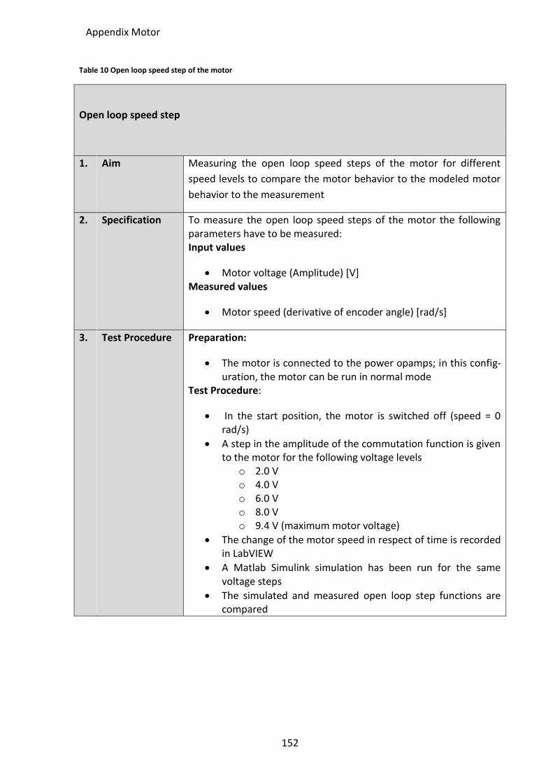
Table 10 Open loop speed step of the motor ........................................................................ 152
Table 11 System frequency response of the motor ............................................................... 153
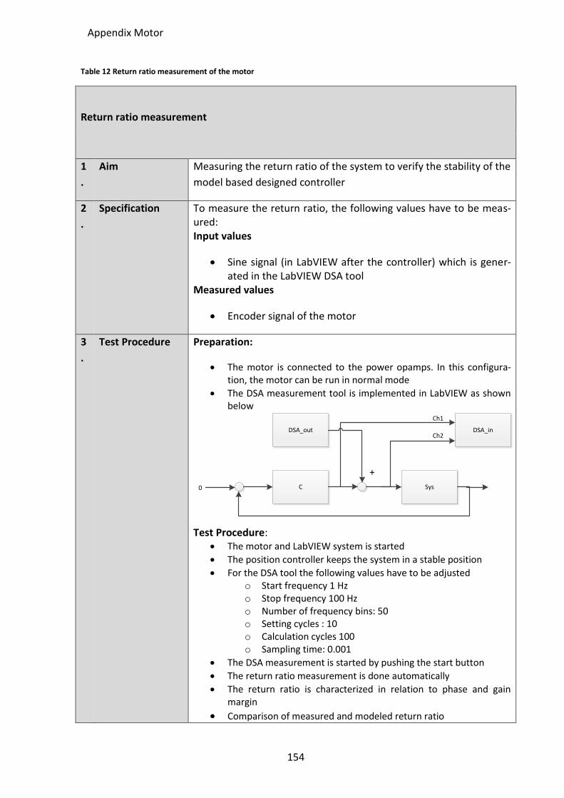
Table 12 Return ratio measurement of the motor ................................................................ 154
Table 13 Step response closed loop of the motor ................................................................. 155
Table 14 Trajectory based positioning of the motor .............................................................. 156
Table 15 System frequency response magnetic bearing........................................................ 172
Table 16 Decoupling verification magnetic bearing ............................................................... 173
Table 17 Return ratio measurement magnetic bearing ......................................................... 174
Page 16
16
Introduction
1 Introduction Brushless DC (BLDC) motors are widely used in many industrial applications due to their ro-
bustness and low maintenance compared to conventional (brushed) DC motors. In addition
their efficiency is very high, which makes these motors interesting in times where a respon-
sible use of resources becomes more and more important. Due to their stiff and compact
design, very high control bandwidths can be achieved. Hence, this motor is often used in
positioning applications.
A second group of actuators which is widely used in industry are reluctance actuators. These
actuators are often used as simple “binary” actuators like solenoid. However they offer line-
ar movement, high force densities and high control bandwidth. As these actuators do not
require a connection between stator and moving part, they are a perfect candidate for high
precision positioning application.
It is important to incorporate both BLDC motors based on the Lorentz principle as well as
reluctance actuators in universities. Students should understand the fundamentals of the
design, building and adjustment of these devices. Brushless DC motors and reluctance actua-
tors are good examples for mechatronic systems due to their close interaction of mechanics,
electronics and control. Using these systems the model based design of mechatronic applica-
tion can be taught. This includes the following details:
Design of BLDC motors including their pole and winding structure
Commutation of BLDC motors including different commutation techniques
Design of reluctance actuators by analyzing the magnetic circuit, as well as calculat-
ing the flux densities and forces in the air gap
System and parameter identification as well as model validation
Loop shaping design of PID controllers
Systems where brushless DC motors and reluctance actuators work in combination are elec-
tro motors with magnetic bearings. Unfortunately, there are no existing solutions of a mag-
netically levitated BLDC motor which can be used for teaching, as commercial systems do
not have access to all the required signals and algorithms. In addition industrial systems are
very price intensive which makes it hard to equip a full lab with such setups.
The goal of this thesis is to develop a modular low cost brushless DC motor with a magneti-
cally levitated rotor. This system should provide access to all the signals, which are needed
to drive, identify and control the motor and the levitation system. The system shall be used
in different levels of teaching, so the various parts need to run separately.
In the design of this system, it is very important to keep the costs low, that universities can
afford this system. The motor has to be produced with standard manufacturing techniques
and low effort like 3D printing. The real-time target NI myRIO will be used as it is cost and
power efficient and can be easily programmed via LabVIEW.
Page 17
17
Introduction
Standard industrial motors uses pulse with modulation (PWM) because their high power
efficiency. The downside of this method for teaching is that it is hard to measure and under-
stand the signals in the motor. For the understanding of brushless DC motors, students have
to be able to measure the signals of the motor by using an oscilloscope, so analog circuits
and signals have to be used. As the focus of this project is set on teaching, the lower power
efficiency of analog amplifiers is less important.
To teach students about BLDC motors, the motor has to have access to all the signals and
algorithms. Block commutation of BLDC motor has to be necessarily possible. In addition the
use of more advanced commutation techniques like sine commutation is desired.
The whole system will be used to teach students about model based design of mechatronic
systems and controllers. Therefore a low design complexity is desired, that it is possible for
students to model the system accurately. In addition there should be a good comparability
between the model prediction and the actual measurement.
One goal of this thesis is to teach students about controller design. The different parameters
of a PID controller can be felt if the torque created by the motor is high enough. A torque of
> 5 mNm should be achieved as a minimum. The speed of the motor is less important, but
should reach a value which is similar to commercial motors which is well above 1000 rpm.
The system has to be designed modular, that it can be used in different levels of studying.
This results in a system which starts with the basics of BLDC motors as the first step, up to
the control of nonlinear MIMO systems in magnetic levitation for graduate level teaching.
The thesis is structure in the following pattern.
In chapter 2, the concept of the brushless DC motor including its magnetic levitation system
is developed. Different concepts of actuation and sensing for the BLDC motor as well as for
magnetic levitation are evaluated. Chapter 3 focuses on the development of an axial field
brushless DC motor. The design of a winding and pole structure is explained and the relevant
motor parameters are calculated. A dynamic model of the motor is created, which is verified
in a number of different tests.
In chapter 4, a three axis magnetic bearing for controlling the Z, Pitch and Roll axis is devel-
oped. Different sensing principles are described. Actuators and power electronics are de-
signed. A dynamic model of the magnetic bearing including position control is created. This
model is verified on the setup by measuring the system behavior.
Chapter 5 describes the design of a magnetic bearing for the two remaining horizontal axes.
A model of the magnetic bearing including all controlled axes is built. Based on the model,
different controllers are tuned. In different tests, the model is verified. In Chapter 6the func-
tionality of the full system is validated. Different tests to show the functionality of the spin-
ning rotor with magnetic levitation are performed. Chapter 7 summarizes the work which is
done in this thesis and gives suggestions for follow-up projects.
Page 18
18
Conceptual design
2 Conceptual design In this chapter, the concept of a BLDC motor with a magnetically levitated rotor is devel-
oped. The defined features from chapter 1 are compared to existing solutions in the field of
brushless DC motors (section 2.1) and magnetic bearings (section 2.2). Section 2.3 compares
different actuator concepts with respect to their applicability and modularity. In section 2.4,
solutions for sensing the rotor position are presented. Section 2.6 presents the overall con-
cept of the motor, to be developed and tested in this thesis.
2.1 Overview brushless DC motors
2.1.1 Basics of DC motors
In conventional (brushed) DC motors permanent magnets are mounted at the stator and
coils are attached to the rotor. This requires a transmission of electric current from the sta-
tionary part of the motor to the rotor which is usually done by brushes. The limited lifetime
of the brushes is the major drawback of conventional DC motors.
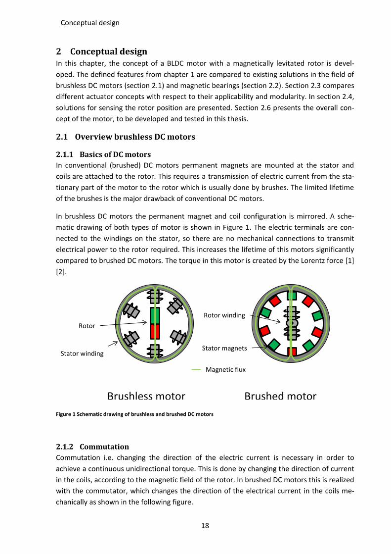
In brushless DC motors the permanent magnet and coil configuration is mirrored. A sche-
matic drawing of both types of motor is shown in Figure 1. The electric terminals are con-
nected to the windings on the stator, so there are no mechanical connections to transmit
electrical power to the rotor required. This increases the lifetime of this motors significantly
compared to brushed DC motors. The torque in this motor is created by the Lorentz force [1]
[2].
Figure 1 Schematic drawing of brushless and brushed DC motors
2.1.2 Commutation
Commutation i.e. changing the direction of the electric current is necessary in order to
achieve a continuous unidirectional torque. This is done by changing the direction of current
in the coils, according to the magnetic field of the rotor. In brushed DC motors this is realized
with the commutator, which changes the direction of the electrical current in the coils me-
chanically as shown in the following figure.
Stator winding
Rotor winding
Magnetic flux
Rotor
Stator magnets
Brushed motor Brushless motor
Page 19
19
Conceptual design
Figure 2 brushed DC motor commutation taken from [3, p. 80]
Using brushless DC motors, the commutation has to be done by motor electronics. The cur-
rent in the stator coils has to be aligned to the magnetic field of the rotor. If this is done cor-
rectly, the electric field rotates in the same speed than the magnetic field of the rotor. To
align the electric current in the coils to the rotor angle, a measurement of the rotor angle is
required [4, p. 4]. This is usually done by Hall sensors, which measure the magnetic field of
the rotor.
Different commutation methods can be chosen to run a BLDC motor. The simplest commu-
tation mode is block commutation. The rotor angle is measured by Hall sensors which gen-
erate binary signals for the motor controller. The controller switches the current through the
motor coils on and off based on these signals (Figure 3 A). Advantage of this method are that
there are low costs for sensing the magnetic angle and the motor software is not complex.
(A) (B)
Figure 3 Bock commutation and Sine commutation
The switching of the current generates torque ripples in the motor. These torque ripples can
be reduced by the use of sine commutation. When sine commutation is used, the rotor angle
has to be measured accurately. The current through the coils is adjusted precisely to the
magnetic field of the rotor to create torque with little torque ripple (Figure 3 B).
Page 20
20
Conceptual design
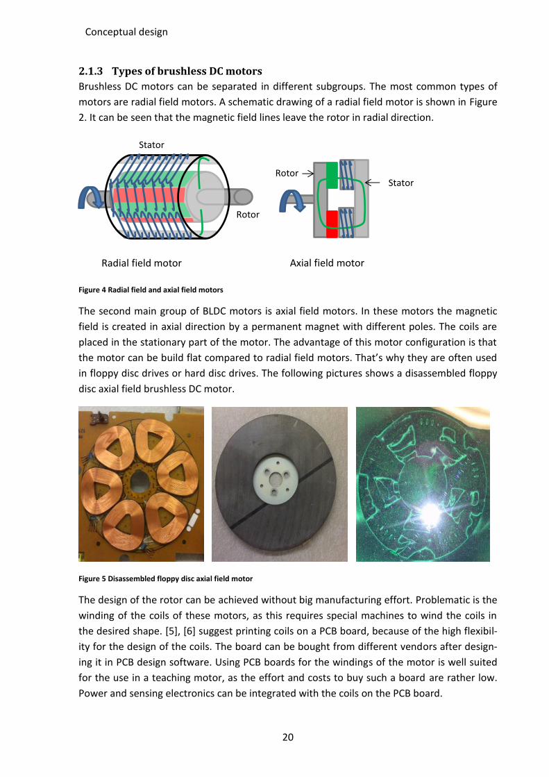
2.1.3 Types of brushless DC motors
Brushless DC motors can be separated in different subgroups. The most common types of
motors are radial field motors. A schematic drawing of a radial field motor is shown in Figure
2. It can be seen that the magnetic field lines leave the rotor in radial direction.
Figure 4 Radial field and axial field motors
The second main group of BLDC motors is axial field motors. In these motors the magnetic
field is created in axial direction by a permanent magnet with different poles. The coils are
placed in the stationary part of the motor. The advantage of this motor configuration is that
the motor can be build flat compared to radial field motors. That’s why they are often used
in floppy disc drives or hard disc drives. The following pictures shows a disassembled floppy
disc axial field brushless DC motor.
Figure 5 Disassembled floppy disc axial field motor
The design of the rotor can be achieved without big manufacturing effort. Problematic is the
winding of the coils of these motors, as this requires special machines to wind the coils in
the desired shape. [5], [6] suggest printing coils on a PCB board, because of the high flexibil-
ity for the design of the coils. The board can be bought from different vendors after design-
ing it in PCB design software. Using PCB boards for the windings of the motor is well suited
for the use in a teaching motor, as the effort and costs to buy such a board are rather low.
Power and sensing electronics can be integrated with the coils on the PCB board.
Radial field motor Axial field motor
Stator Rotor
Stator
Rotor
Page 21
21
Conceptual design
2.2 Overview magnetic bearings
2.2.1 Reluctance actuators in magnetic levitation
Magnetically levitated systems based on reluctance actuators are often used in universities
as a mechatronic example of magnetic actuators and controller design for nonlinear sys-
tems. The aim of these teaching projects is to levitate a ball in a constant distance to an ac-
tuator. Teaching applications of magnetic levitation using this physical principle of applying
forces against gravity are [7], [8], [9] or [10]. A schematic example is shown in the following
figure.
Figure 6 Schematic view of a reluctance actuator based magnetic levitation system
By applying a current I through a coil which is wound around iron core a magnetic flux Φ in
the actuator is created. This result in a flux density B and a force 𝐹𝑚𝑎𝑔 in the air gap between
actuator and mover (steel ball). The current through the actuator is controlled based on the
measured position of the steel ball. The position is often measured by optical sensors.
The force characteristic of this actuator can be described with the following equation, where
x represents the distance between actuator and steel ball and k a geometry specific con-
stant.
𝐹𝑚𝑎𝑔 = k ∙𝐼2
𝑥2
Equation 2-1
By the use of one reluctance actuator, only attraction forces between stator and mover
(steel ball) can be applied. In the above configuration the negative forces are generated due
to gravity. Using this concept the steel ball can be actively controlled in one degree of free-
dom. If more DOF have to be controlled, as it is the case in this thesis, more reluctance actu-
ators can be used. The University Saarland [11] developed a magnetically levitated plate,
Steel
Steel
Fg
I
𝛷
x
z
Fmag
Page 22
22
Conceptual design
where four reluctance actuators are placed at the edges of the plate. Using these actuators
the Z, Pitch and Roll axis can be controlled and the gravity is compensated. This approach
seems interesting for the levitation of the horizontal axes of the rotor.
2.2.2 Magnetic bearings
Electric motors with magnetic bearings can be separated in two main groups. The first group
comprises motors with magnetic bearings. The magnetic bearing is independent from the
motor windings itself. A second group is called bearingless motors in which the generation of
torque and radial forces is combined [12]. Bearingless motors will not be considered in this
thesis as they do not allow a modular design concept of the system.
Figure 7 shows a typical structure of a motor system with conventional magnetic bearings.
The motor itself is placed between two radial magnetic bearings. The force created by each
radial bearing is perpendicular to the shaft position. This way the rotor can be centered in
the middle. The position of the Z axis is regulated by a thrust magnetic bearing.
Figure 7 Motor with magnetic bearings picture taken from [12, p. 3]
Typically each radial magnetic bearing has four coils around the stator, two in the X axis and
two in the Y axis working in an antagonistic arrangement. So it is possible to create forces in
the positive and negative direction of each axis to keep the rotor in its position. This is espe-
cially positive when there is no gravity force to readjust the system in negative direction. The
motor itself can be used and controlled as a conventional electric motor without any mag-
netic bearings.
The antagonistic arrangement of the actuators is reasonable for axis, where there are no
readjusting gravity force is in the system. For the case of an axial field motor, this configura-
tion has to be preferred for horizontal axis.
Page 23
23
Conceptual design
2.3 Actuation concept
With the defined features and considerations about brushless DC motors and magnetic bear-
ings, different concepts of BLDC motors with magnetic bearings are developed in order to
achieve a good overall design.
An axial field brushless DC motor on a PCB board as suggested in [5] is chosen because the
windings are the critical part in building the motor. This can cleverly be solved by printing
them on a PCB board in combination with the rest of the electronics.
Reluctance actuators above the rotor as advised in [11] will be used to control the vertical
axis of the rotor, working against gravity. For the horizontal axis, where no gravity force can
be used, an antagonistic arrangement as suggested in [12] is developed.
2.3.1 Vertical actuation
The actuation of the Z, Pitch and Roll axis can be done similar to the levitation of a plate in
2.2.1 by mounting reluctance actuators above the rotor. Because of the gravity force of the
rotor, only one direction of actuation is required. For the control of the three axes, only
three actuators are needed which fits to the limited D/A channels of the myRIO. Also the
amount of power electronics can be reduced with this configuration.
Actuator designs which can control these three axes of the rotor are described in Figure 8.
All concepts use three reluctance actuators which are mounted above the rotor in an angle
of 120°. The magnetic flux created by these actuators is indicated with green lines.
Figure 8 Actuator concept for Z, Pitch and Roll
In (A) three reluctance actuators are mounted above the rotor which are connected via a
return path above the other actuators. This results in a simple design. Negative in this actua-
tor configuration is, that there are strong couplings between the actuators. When the cur-
(A) (B) (C)
R31 R32 R33
A31 A32 A33
R34R21a
A21
R22a
A22
R23a
A23
R21b R22b R23b
R11 R12 R13
A11 A12 A13
Page 24
24
Conceptual design
rent in one actuator is increased, the magnetic flux and force increases in all three actuators.
This makes this configuration hard to control.
(B) shows a concept where the three reluctance actuators are separated from each other.
Couplings in the magnetic flux between the actuators are avoided. The disadvantage in this
concept is that each actuator has two points where a force is created at the outer radius
which is not wanted. When the rotor tips or tilts, the force generated by one actuator moves
between the two stator coils of the actuator, as the resistances changes unequally. This re-
sults in an additional nonlinear behavior.
In configuration (C) a feedback path (R34) in the middle of the rotor is added. During a nor-
mal operation, the magnetic flux created by each actuator is over the feedback path in the
middle. So the actuators can be driven mostly independent form each other.
By comparing these three actuator principles it can be seen, that concept (C) offers the most
advantages for controlling the Z, Pitch and Roll axis, as the couplings between the actuators
are low. In addition the points of force generation are constant.
2.3.2 Horizontal actuation
For the control of the X and Y axis additional actuators have to be added. As there is no grav-
ity force in the X-Y plane, an antagonistic actuator principle has to be chosen as it is pro-
posed in 2.2.2 to be able to apply positive and negative forces to the rotor. [12] suggests
using two reluctance actuators in each axis to achieve an antagonistic actuation, which re-
sults in four actuators for the X-Y plane. Problematic for the use of four actuators is the limi-
tation of D/A channels on the myRIO. So actuator principles using three actuators for the X-Y
plane actuation are developed.
Figure 9 Actuation concept for the X and Y axis
Rh1
Rv1 Rv2Ah1
Av1
R1 R2R3
A11 A12
Rh11 Rh12
Ah1
z x
(A) (C)
y
x
(B)
x z A
v1
Ah1
A11
A12
Ah2
Ah1
Ah3
Page 25
25
Conceptual design
To achieve forces which are distributed equally in the X-Y plane the three additional reluc-
tance actuators are also mounted in an angle of 120° around the rotor. Figure 9 shows three
different concepts for controlling the X and Y axis.
The first concept (A) adds a reluctance actuator in the X-Y plane next to each Z axis actuator.
By changing the current through this actuator Ah1 the rotor can be controlled in X and Y. As
the magnetic circuit of the horizontal axis actuator is designed to be over the feedback path
(RV2) in the middle of the rotor, also a force in the Z axis is created, which needs to be com-
pensated. In addition there is a coupling between the horizontal axis actuators and the verti-
cal axis actuators in the magnetic flux.
Concept (B) shows a more integrated version for the control of the X-Y plane. Two actuators
are mounted in an angle of 45° above the rotor where a triangular shaped ring is added.
With changing the current in these actuators antagonistically positive and negative forces in
the X and Y axis can be applied. By changing the current through both actuators in parallel, a
force in the Z axis as well as a torque at the rotor is applied. This can be used to control the
Z, Pitch and Roll axis. Negative in this concept is, that the magnetic flux created by the actua-
tors can be shortened. When the rotor turns out of its middle position and the resistance R2
becomes lower than R3 which results in a force mainly in Z direction. Then a creation of
forces in the X and Y axis by changing the current antagonistically is not possible and more
complex algorithms have to be used.
In concept (C) three reluctance actuators are mounted around the rotor. By applying a cur-
rent through one actuator (Ah1 – Ah3), a force in its direction is created. Because of the angle
of 120° between the actuators, positive and negative forces in X and Y can be generated. To
keep the point of actuation for each actuator centered, the distance between both force
creating parts of one actuator is set to be small. Positive in using this concept is that the X
and Y actuators can be used separately from the vertical actuators, which results in a higher
possibility of modularization as well as in easier control algorithms. In this concept two
points of forces are created by each actuator. The distance between these two points is set
to be low, to reduce the effect of the varying center of force per actuator.
For the purpose of this thesis concept (C) offers the most advantages because the couplings
between the vertical and horizontal axis are low as it would be the case in concept (A). Also
there is no possibility to shorten the magnetic flux as it would be the case in concept (B).
Page 26
26
Conceptual design
2.4 Sensor concept
2.4.1 Sensing of the motor angle
In the basic configuration of the motor, commutation as well as position control has to be
possible. Because of the modular design of the motor, a contactless measurement of the
rotor position needs to be done.
The position sensing of the rotor in BLDC motors is often done by using quadrature encod-
ers. An example of an optical based encoder is shown in Figure 10. On the rotor a disc with
different slots is mounted. Via a LED and light receiving elements, quadrature signals are
generated when the rotor is rotating.
Figure 10 Optical quadrature encoder, picture taken from [13]
The resolution of the encoder is based on the amount of slots on the encoder disc. To in-
crease the resolution of the encoder, analog sine/cosine encoders can be used where the
position between each slot is interpolated. The signals of both types of encoder are shown in
Figure 11.
For the design of position controllers with a sufficiently high control bandwidth as well as for
system identification it is required to measure small angle changes of the rotor (< 1°). When
a quadrature encoder is used, this results in more than 90 segments of the encoder disc. This
high amount of slots in a disc is hard to produce with standard manufacturing techniques.
When a sine/cosine encoder is used, which interpolates the values between each segment,
the number of segments to achieve a high resolution encoder can be reduced significantly
and the encoder disc becomes much easier to manufacture.
Page 27
27
Conceptual design
Figure 11 Encoder signals of quadrature and sine/cosine encoders
As the encoder is also used for commutation of the BLDC motor a reference signal of the
magnetic angle of the rotor has to be measured and both signals have to be aligned in order
to get a good commutation. In industrial application the measurement of the magnetic angle
is usually don be three Halls sensors which measures the magnetic field for each phase and
generate binary values for the real-time target.
[14] suggests to use permanent magnets and Hall sensors to build an incremental encoder
for measuring the rotor position. When the magnetic field of the motor magnets is used to
create a sine/cosine encoder, the measurement of the magnetic angle and the rotor position
can be combined. Also no additional cost for creating an encoder disc is required. Using this
combination a cheap and accurate sensor for both cases of application can be built.
2.4.2 Position sensing for magnetic bearings
The magnetic bearing works with closed loop control, that’s why an accurate measurement
of each axis needs to be done. Because of the different stages of modularization, two set of
sensors should be used to measure the vertical and horizontal axes independently. Sensors
which are not sensitive to magnetic fields should be used to avoid disturbances caused by
the magnetic fields of rotor and the reluctance actuators.
The sensors of the Z, Pitch and Roll axis are placed above the rotor close to the actuators as
it is shown in Figure 12. Using this configuration the height of the rotor is measured at three
points. This makes it possible to control each actuator individually with the measured dis-
tance between actuator and sensor. A second option is to transform the measured distances
in Cartesian coordinates and to control the different axis.
Page 28
28
Conceptual design
Figure 12 Sensor concept of the magnetic bearing
For the placement of the sensors of measuring the position in X and Y the same approach is
chosen. The sensors S4 – S6 are placed next to the actuators and measures the distance be-
tween actuator and rotor. So a control of each actuator independently via the measured
distance between actuator and rotor is possible. In addition the sensors value can be trans-
formed in Cartesian (X, Y) coordinate. When this is done three the sensors offers a higher
accuracy because only two sensors are required to measure these axes. The third sensor acts
redundant.
2.5 Rotor concept
The rotor of the BLDC motor has to be designed, that permanent magnets can be glued onto
the bottom. Therefore a smooth surface between rotor iron an magnets is required in order
to reduce the magnetic flux in these points. To achieve high dynamics with the motor, as
well as to reduce the bias current to levitate the rotor, a mass of the rotor has to be low.
For levitating the rotor in its desired position, the ferromagnetic surface of the rotor, which
interacts with the reluctance actuators, has to be big enough, that no additional resistance
between in the magnetic circuits appear. In addition a material with a high permeability has
to be chosen.
x
y
z
A3
A2
A1
A4
S4
S5
S6
A5
A6
S3
S2
S1
Page 29
29
Conceptual design
As the vertical and horizontal axes have to be used independently, the couplings between
these axis has to be low. This can be achieved, when the horizontal axis actuators are acting
in the center of gravity.
The reluctance actuator of the horizontal axes has to be placed close the permanent mag-
nets of the rotor. Nevertheless the rotor has to be designed, that the cogging torque be-
tween rotor magnets and actuators is low. In the following figure, the requirements in the
rotor design are shown.
Figure 13 Rotor concept
2.6 Concept for a Maglev BLDC motor
2.6.1 BLDC motor
An axial field motor is designed with all the electronics and windings placed on a PCB board.
The rotor consists of a round steel disc with glued on permanent magnets. To measure the
rotor position accurately for control and commutation a Hall sensor based sine/cosine en-
coder is implemented on the board.
In this step of modularization different commutation techniques of BLDC motors can be
shown. Also the processing of sensor signals can be explained. The motor characteristic pa-
rameters can be measured and compared to calculated values which have been used the
model based design approach. Finally a position control of the rotor axis can be designed
and tested.
Figure 14 Motor with and without back iron
Center of gravity No cogging
Low mass, high permability
Back iron
Bea
rin
g
PCB Back iron (steel)
Rotor (steel)
No back iron
Bea
rin
g
PCB
Magnetic flux in the motor Magnetic leakage flux
Rotor (steel)
Page 30
30
Conceptual design
Because of the modular design it is required to replace the rotor with conventional bearing
to the rotor with magnetic bearings. This has to be done without a big effort, which results in
a motor without back iron which is described in Figure 14 . The attraction forces between
rotor and back iron would make it had to replace the rotor and would increase the force to
levitate the rotor significantly. On the other hand the torque generated by the motor is low-
er because of the high leakage flux and the bigger magnetic resistance. The following figure
shows the desired design of the BLDC motor on a PCB board and an easy connection to the
myRIO real-time target.
Figure 15 Schematic drawing of the motor concept
2.6.2 Magnetic levitation
The second goal of this project is to make the rotor disc levitating using reluctance actuators.
In this configuration it is possible to levitate the rotor in up to five degrees of freedom (X, Y,
Z, Pitch and Roll). Different control algorithms and interactions between different axes can
be observed and algorithms to prevent these effects can be explained.
This is realized by adding three actuators above the rotor in an angle of 120°. These actua-
tors take off the gravity and control the Z, Pitch and Roll axis as it is described in 2.3. A con-
cept for sensing the rotor position is developed in 2.4.2. The placement in the setup is shown
in Figure 16.
To stabilize the X and Y axis, three more actuators and sensors are added around the rotor as
it can be seen in Figure 16. In this configuration the position in the X and Y plane can be ad-
justed and imbalances of the spinning rotor can be compensated. With this configuration it
is possible to control the rotor disc in five DOF using the magnetic bearing.
Rotor disc in-
cluding perma-nent magnets
NI myRIO
Power- and sensing electronic
Position sensing
PCB including motor windings
Page 31
31
Conceptual design
2.6.3 Magnetically levitated BLDC motor
In the final step the BLDC motor with magnetic bearing can be used. So the motor can be
driven magnetically levitated and in six axes controlled. Different effects, like sensor noise
because of the rotating rotor and gyroscopic effects can be seen.
Figure 16 Concept of the magnetic levitated brushless DC motor
Hall sensor for measuring the rotor position
X, Y sensors
Z, Pitch, Roll sensors
Rotor
Z, Ptich
, Ro
ll actuato
r
Z, Ptich
, Ro
ll actuato
r
Page 32
32
Axial field brushless DC motor
3 Axial field brushless DC motor This chapter describes the design, modeling and testing of an axial field brushless DC motor.
Section 3.1 focuses on the coil design of axial field brushless DC motors. Different winding
structures are compared and rated regarding their usability in PCB motors. In section 3.2 the
rotor of the BLDC motor is developed. Different types of permanent magnets and their use
in axial field motors is compared.
The accurate sensing of the rotor position using Hall sensors is explained in section 3.3. For a
model based design approach, the motor characteristic parameters are calculated in 3.4 in
order to predict the relevant motor behavior.
In section 3.5 the motor is designed including electronics and LabVIEW implementation.
With the designed motor, the estimated motor parameters are verified in section 3.6.
For the design of position controllers a dynamic model of the BLDC motor is developed and
linearized in section 3.7. A position controller is designed and the implementation of a tra-
jectory based positioning developed. In section 3.8 the model and controller is validated.
3.1 Coil design
The following section compares different winding structures of brushless DC motors. These
structures are compared regarding their use in PCB motors. For the chosen winding struc-
ture, coils are designed which offer a high torque capability.
3.1.1 Winding structure
The winding structures of BLDC motors can be separated in two groups, overlapping and
non-overlapping windings. The two different structures are described and compared for the
use in PCB motors.
3.1.1.1 Overlapping winding
The overlapping winding is the most common winding structure in standard synchronous
motors, as the magnetic field in the air gap of the motor is nearly sinusoidal [15, p. 2]. In this
type of winding the coils of the different phases are overlapping. So the coils of the different
phases have to be separated to different layers on the PCB board. An example of an over-
lapping winding with four coils per layer is given in the following figure.
Page 33
33
Axial field brushless DC motor
Figure 17 Overlapping winding structure
In the overlapping winding structure the number of coils per phase 𝑁𝑐𝑜𝑖𝑙𝑝𝑒𝑟𝑝ℎ𝑎𝑠𝑒 is equal to
the number of poles at the rotor 𝑁𝑃𝑜𝑙𝑒𝑠 as displayed in Equation 3-1. The total amount of
coils of the motor is calculated by number of coils per phase multiplied with the number of
phases.
𝑁𝑐𝑜𝑖𝑙𝑝𝑒𝑟𝑝ℎ𝑎𝑠𝑒 = 𝑁𝑃𝑜𝑙𝑒𝑠
Equation 3-1
The difference between electrical speed 𝜔𝑒𝑙 and mechanical speed of the motor 𝜔𝑚𝑒𝑐ℎ is
represented in the following equation.
𝜔𝑚𝑒𝑐ℎ =𝜔𝑒𝑙 ∙ 2
𝑝
Equation 3-2
The variable p is the number of poles at the rotor. The following table shows the number of
poles, the resulting coils and the ratio between mechanical and electrical speed for a three
phase motor.
Table 1 Parameter setup for overlapping windings
Poles Coils Ratio 𝝎𝒆𝒍/𝝎𝒎𝒆𝒄𝒉
2 6 1
4 12 0.5
6 18 0.33
8 24 0.25
10 30 0.2
Page 34
34
Axial field brushless DC motor
For the design of brushless DC motors on PCB boards it has to be taken into account, that
every coil must have an even number of layers, to have a connection through the lead cables
from the outside of the coil. Otherwise an extra connecting layer is needed. This is shown in
the figure below. This results in a minimum of six layers of the PCB board for a three phase
motor.
Figure 18 Layers per Coil
As the coils of the different phases are overlapping, the connection between the different
layers is difficult. It can either be done by using “not through hole connections”, which are
expensive to manufacture, or by leaving enough space in the other coils to use standard
“through hole connections” which lowers the amount of turns of a winding. Differences be-
tween both connection types are shown in the figure below.
Figure 19 Through hole and not through hole connection
3.1.1.2 Non Overlapping winding
In comparison to the overlapping winding structure the coils are separate in the non-
overlapping winding structure. This winding structure is a common structure in linear motors
and for the building of low speed torque motors [16]. The following figure shows a schemat-
ic view of a non-overlapping winding. It can be seen, that every coil is independent from the
other coils.
Lead wire 1
(Layer 1)
Lead wire 2
(Layer 2) Layer connection
Layer connection
Lead wire 1
(Layer 1)
Lead wire 2
(Layer 2)
Through hole connection
Not through hole connection
Layer 1
Layer 2
Layer3
Layer 4
Page 35
35
Axial field brushless DC motor
Figure 20 Schematic view of non-overlapping windings
The relation between the electrical and the mechanical speed in Equation 3-2 still holds.
Common coil and pole arrangements for non-overlapping windings structures are three coils
to four poles or three coils to five poles configurations and their multiples. The following
table gives an example of common distributions and their ratio between electrical and me-
chanical speed.
Table 2 Parameter setup for overlapping windings
Poles Coils Ratio 𝝎𝒆𝒍/𝝎𝒎𝒆𝒄𝒉
4 3 0.5
8 6 0.25
10 6 0.2
The advantage of a non-overlapping winding structure in the design of an axial field PCB mo-
tor is the high design flexibility in designing the coils. For the amount of layers on the PCB
board only an even value has to be chosen because of the lead cables. So the torque con-
stant of the motor can be adjusted better by adding or removing two layers on the board.
The connection between the different layers on the board can be done by “through hole
connections” which makes the board less expensive.
3.1.1.3 Winding comparison
By the use of a non-overlapping winding structure there is more flexibility in designing coils.
This way the layers of the board can be adjusted freely and the number of turns can be ad-
justed to the maximum allowable resistance of the coil. In addition the costs for producing
the boards are lower because of the possible “through hole connection”. For this reasons a
non-overlapping winding structure has been chosen for the design of the motor.
Page 36
36
Axial field brushless DC motor
3.1.2 Coil Design
To achieve a high torque capability in the motor using little mechanical space, it is important
to design coil which are effective in respect of their shape. To maximize the torque crated by
each coil, the length l of wires in radial direction to the rotating axis has to be maximized.
These wires create the motor torque via the Lorentz force F when a magnetic field B is ap-
plied. The following figure shows a simplified coil structure and the forces due to current and
magnetic field.
Figure 21 Lorentz forces in a coil
One approach in the design of coils with high torque is the use of rhomboidal turns (Figure
22 A) in the coils. This way the length of wire in the magnetic field can be maximized. On the
other hand the 𝑅 ∙ 𝐼2 losses in the coils are very high, as there is only half of the coil in the
magnetic field [5, p. 40]. Also this coil structure needs a lot of space on the PCB board, which
makes it inefficient in respect of space.
Figure 22 Rhomboidal coil, coil with parallel active sections, picture taken from [17, p. 2]
A second approach is the use of coils with parallel active sections (Figure 22 B). In compari-
son of the maximum achievable torque under a magnetic field, the torque created by the
Lorentz force is lower. But on the other hand a higher torque constant in relation to the used
space on the PCB board and to the resistance of the coil can be achieved, which makes this
shape attractive.
For the design of the PCB motor the coils with parallel active sections are chosen, as this coil
arrangement is more efficient in relation of space and copper losses.
l
I
B
F
A B
Page 37
37
Axial field brushless DC motor
An important design parameter of the coil is the number of turns which can fit on one coil.
This parameter is estimated by using the following equation [17, p. 4]:
𝑁 =𝑅𝑜 − 𝑅𝑖
2 ∙ (𝑤 + 𝑐)
Equation 3-3
The variables 𝑅𝑜 and 𝑅𝑖 represents the outer and inner radius of the coil. N is the total
amount of turns at one layer. With a track width of 5 mil and a clearance of 6 mil on the PCB
board, an outer diameter of 75 mm and an inner diameter of 20 mm of the coils, each layer
of the coil is estimated to have 49 turns.
To achieve a higher torque more layers of coils have to be used and the coils of the different
layers have to be connected in series. In order to have the electrical current in the same di-
rection in each coil, the coils of the different layers have to be designed as the following fig-
ure indicates.
Figure 23 Coil structure for different layers, picture taken from [17, p. 2]
With the first approximation of the coil parameters and the consideration about connecting
different layers, a more detailed coil version has been created. A Matlab script for the design
of coils is written which is attached at the appendix. This script is interfaced to the PCB de-
sign software Altium where the needed Gerber files and the rest of the electronics are de-
signed.
It turned out, that a maximum amount of 35 turns can be placed on one coil and one layer.
By using a four layer PCB board 140 turns can be achieved on one coil. The torque constant
of each coil can be calculated using Equation 3-18.
To achieve the maximum torque constant in relation to the needed space, different varia-
tions of coils with parallel active sections have been calculated. It turned out, that the maxi-
mum torque of the motor can be increased by 17 % using coils with an arc structure at the
outer radius compared to coils with only straight lines at the outer radius. This is because the
maximum length of the tracks parallel to the rotating axis can be enlarged using the arc
structure. This can be seen in Figure 24.
That’s why coils with parallel active sections and an arc structure at the outer radius have
been chosen in the coil design of the motor.
a) b)
Page 38
38
Axial field brushless DC motor
Figure 24 Coils with straight lines and arc structure
3.2 Rotor design
After designing the coil structure of the motor a rotor is designed to get a motor with a high
torque capability and easy manufacturing. Therefore different magnetic materials are com-
pared and tested. The most promising design is chosen.
3.2.1 Magnetic material
To achieve a motor with adequate torque, different magnetic materials are compared. The
main requirements for the design of the rotor are that the magnets can be either bought as
a standard magnet, or that the permanent magnet material can be magnetized and ma-
chined with adequate effort. Also the magnetic field created by the magnets has to be suffi-
ciently high. Table 5 in the appendix shows different magnetic materials and their main
properties.
It can be seen, that NdFeB magnets offer the highest energy product, but on the other hand
they are hard to machine and remagnetize. This means, that this type of magnetic material
can only be used if the suitable shape of NdFeB magnets is available of the shelf. Fortunately
there is a wide range of different shapes of NdFeB magnets, which can be bought from dif-
ferent vendors.
Ferrite magnets would be a good solution for the use in rotors for axial field machines, as
they can be remagnetized rather easy, and still offer a high magnetic field. Unfortunately no
ferrite ring magnet with the right dimensions could be found.
Arc shaped Straight lines
Page 39
39
Axial field brushless DC motor
NdFeB flexible magnets and NdFeB bonded magnets are also not the best choice for the de-
sign of a prototype of an axial field rotor, as even if they can be machined it is hard to mag-
netize the rotor in the desired pattern. On the other hand, if a larger amount of motors is
planned to be built, bonded NeFeB magnets could be a good choice, as they can be bought
machined and magnetized from different vendors. For large amounts of motors this kind of
magnet offers high energy product as well as customized shapes.
A flexible ferrite magnet offers the lowest energy product, but they can be machined and
magnetized very easy for prototyping of different shapes and magnetic patterns. Because of
this features, this material becomes interesting for the use in prototypes of an axial field
brushless DC motor.
It can be seen, that NdFeB magnets and ferrite flexible magnets offers the most advantages
for a first prototype of an axial field brushless DC motor. Rotor configurations of these two
rotor systems will be discussed in the next steps.
3.2.2 Flexible magnet rotor
For building a flexible magnet rotor a sheet of flexible magnetic material has been ordered.
With a magnetic material listed in Table 5 and a given thickness the magnetic flux density in
the PCB board of the motor can be calculated. The magnetic circuit of the motor with a back
iron behind the rotor can be represented as the schematic shown in Figure 25.
Figure 25 magnetic circuit of a motor with back iron
The magnetomotive force Θ created by the permanent magnets can be calculated using the
following equation.
Θ = 𝐻𝑃𝑚 ∙ 𝑙𝑝𝑚
Equation 3-4
Θpm
Rpm
Rair
Θpm
Rpm
Rair
Rfe
Rfe
Rpcb Rpcb
Page 40
40
Axial field brushless DC motor
The variable 𝐻 represents the magnetic flux intensity of the permanent magnet and l the
length of the magnet. The magnetic resistance 𝑅𝑚 of the different elements in the magnetic
circuit can be expressed as:
𝑅𝑚 =𝑙
𝜇0 ∙ 𝜇𝑟 ∙ 𝐴
Equation 3-5
Where µ0 is the magnetic permeability on vacuum, µr is the magnetic permeability of the
material and A the cross section. With the sum of the resistances and the magnetomotive
force, the magnetic flux Φ can be calculated.
Φ =Θ
𝑅𝑚𝑡𝑜𝑡
Equation 3-6
The flux density B in the PCB board can be determined as:
B =Φ
𝐴
Equation 3-7
The variable A represents the cross section in the PCB board in the magnetic field. According
to these calculations a flux density of 0.08 T can be achieved using a flexible magnet disc
with a length of 3 mm.
In order to magnetize the rotor in the desired magnetic pattern a magnetization tool using
NdFeB permanent magnets has been developed which is shown in the figure below.
Figure 26 CAD Magnetizing tool
Using this tool a pole structure of eight poles can be placed on the sheet of flexible perma-
nent magnets. To magnetize the flexible magnets, the rotor will be clamped in a lathe. On
the ram of the lathe the magnetizing tool is clamped. To magnetize the rotor the following
steps have to be performed:
Return Iron
Retor back iron
flexible magnet
Lathe
Magnetizing magnet
Return iron
Ram
Page 41
41
Axial field brushless DC motor
Lowering the distance between the flexible magnet and the magnetizing tool, until
both sides almost touch
Turning the spindle of the lathe at least 45° by hand (the spindle has to be turned
clockwise)
Increasing the distance between the two sides till the magnetic field between the
two parts is negligible
Removing the rotor from the lathe
The magnetization process is shown in the following figures.
Figure 27 magnetizing a flexible magnet rotor
To calculate the needed magnets in the magnetization tool Equation 3-4 to Equation 3-7
have been used. According to these calculations a NeFdB magnet with a length of at least 12
mm has to be used to generate a magnetic field higher than 1.0 T which is desired to achieve
full remagnetization in the flexible magnet.
To validate the magnetic patterns on the rotor a magnetic foil has been used, which shows
the different magnetic field lines. In Figure 28 it can be clearly seen, that the rotor has the
desired pole distribution of 8 poles.
Figure 28 Self magnetized flexible magnet rotor
Page 42
42
Axial field brushless DC motor
3.2.3 NeFdB magnet rotor
The second design approach for a low cost rotor with off the shelf material is done by using
NeFdB disc magnets which are glued on a ferromagnetic steel disc. NeFdB magnets have
been chosen for this purpose as they can be bought from many vendors.
Different disc magnet configurations have been calculated to achieve the maximum amount
of magnets on a rotor disc with a diameter of 75 mm. It turned out, that a magnet configura-
tion of round magnets with a diameter of 13/16’’ gives the highest density of permanent
magnets, without using too many magnets. The following figure shows the CAD drawing of
the designed magnet.
Figure 29 CAD drawing of a NeFdB magnet
Round magnets have the additional advantage, that the magnetic field of a rotation rotor is
expected to be more sinusoidal, than by the use of rectangular magnets. This is indicated in
the following figure where the magnetic field for one turn of the windings is estimated.
Figure 30 Expected magnetic field in the coils
As the magnetic field of this rotor is strong enough to be used as a motor with and without
back iron, the magnetic flux density for both cases has been calculated. According to Equa-
tion 3-4 to Equation 3-7 the magnetic field in the PCB board is 0.6 T using a back iron and
NeFdB magnets with a length of 3 mm.
Sine behavior
Expected magnetic
flux density behavior
Page 43
43
Axial field brushless DC motor
For calculation of the magnetic field in the PCB board using no back iron the 2D FEM simula-
tion program FEMM is used. In this software a 2D model of the rotor is created. According to
this simulation the magnetic field in the PCB board is averaged at 0.23 T. A figure of the
simulated magnetic field is shown in Figure 31
Figure 31 2D Magnetic field simulation of the motor without back iron
When building a rotor with glued on permanent magnets it turned out, that it is very im-
portant that the magnets are placed correctly. Variations on the placement will affect the
Hall sensor reading negatively and create imbalances on the rotor. For an accurate place-
ment of the magnets on the rotor iron, a mounting tool has been designed and 3D printed. A
picture of the placement tool and the designed rotor is shown in the following figure.
Figure 32 NdFeB magnet placement tool and NdFeB rotor
The rotor has been manufactured according to the CAD files attached in the appendix.
3.2.4 Comparison of the rotor configurations
Two different rotor configurations have been designed. Depending on the purpose of the
motor application it can be decided, which meets the specifications better. For a teaching
motor, it is suggested to use NdFeB magnet, as this type of rotor offers a higher torque ca-
pability, even if it is used without a back iron under the PCB board.
PCB board
Airgap PM Rotor iron
Page 44
44
Axial field brushless DC motor
3.3 Position sensor
For commutation of the motor current as well as for position control of the motor, a position
sensor has to be implemented, as it is described in chapter 2.4.
Two hall sensors are measuring the magnetic field which is exposed by the permanent mag-
nets of the rotor. The Hall sensors are placed in a 22.5° angle mechanically, which is an angle
of 90° in magnetic field.
When the rotor is spinning, the magnetic field should change in sinusoidal shape. The fre-
quency of the magnetic field is four times the mechanical rotor frequency because of the
eight poles (four pole pairs) on the rotor. This way one mechanical rotation of the motor
angle 𝜑 results in four rotations in magnetic angle 𝜑𝑚𝑎𝑔 as it is shown in the following equa-
tion.
𝜑 =𝜑𝑚𝑎𝑔
𝑝/2
Equation 3-8
The following figure shows the rotor with the different poles and the desired signal sensor
curve.
Figure 33 Sine/cosine encoder reading
To calculate the magnetic angle of the rotor, the arctan between the sine signal (A) and the
cosine signal (B) has to be build.
𝜑𝑚𝑎𝑔 = tan−1 (
𝐴
𝐵)
Equation 3-9
For efficiency reasons, the atan2 function is used, as this function takes care of the four
quadrants of the signal.
𝜑𝑚𝑎𝑔 = 𝑎𝑡𝑎𝑛2(𝐴, 𝐵)
Equation 3-10
The value range of the atan2 function is –π to π. To measure the total magnetic rotation of
the rotor the numbers of rotations have to be counted and added to the previous value.
H
22.5°
Page 45
45
Axial field brushless DC motor
For the placement of the sensors, they have to be in the magnetic field of the permanent
magnets, but not in the field of the coils, as this would disturb the measurement of the rotor
angle. So the sensors are placed outside the coils as shown in Figure 33.
When the sensor is placed at a distance of 3 mm next to the rotor, the magnetic flux density
in the sensors changes between +0.13 T to -0.13 T according to the FEMM simulation which
is shown in Figure 34. This results in a change of the output voltage of the Hall sensors of
more than 3 V [18].
Figure 34 Simulated min/max flux densities in the Hall sensors
The voltage change is sensed by the 12 bit A/D channels of the myRIO system. Caused by the
quantization of the real-time target, one magnetic rotation can be sensed with roughly 2500
steps. If the sine behavior is ideal, and there is no noise on the signal, this results in a sensor
resolution of 0.04° which shows, that the positon can be sensed using this concept with high
resolution . Because of non-linearity in the sine behavior and sensor noise, the accuracy will
be lower.
The processing of these sensor values is put on the FPGA of the myRIO real-time target, in
order to save recourses of the microprocessor and to lower time dependencies. Additionally
the resolution of the sensing can be increased by oversampling on the FPGA and averaging
the signals via a low pass filter.
If a higher accuracy of the rotor position measurement needs to be done, a sine/cosine en-
coder using photo resistive elements and LED in addition to a 3D printed slotted disc can be
added to the rotor. An example of such a encoder is shown in Figure 40.
NdFeB magnet
Rotor irion
Hall sensor
Page 46
46
Axial field brushless DC motor
3.4 Parameter calculation
In the design of motors it is very important to know the motor behaviors like maximum
torque, maximum speed, current trough the coils and different time constants in advance.
These data can be calculated with the motor geometry and material specific constants. By
knowing about these parameters, the motor which has to be designed can be matched per-
fectly to the desired application by a model based design approach.
In this section the motor specific parameters of axial field brushless DC motors will be calcu-
lated, and the equations for specific parameters are discussed.
3.4.1 Torque constant
To calculate the maximum achievable torque of the motor, the torque constant is calculated.
The torque constant represents the relation between applied current and torque of the mo-
tor. The torque in the motor is created by the Lorenz force. For the calculation of the total
torque, the torque which is created by each wire is calculated and the different values are
summarized. The Lorentz force which is created by each wire is calculated based on the fol-
lowing equation.
𝐹 = 𝐼𝑥𝐵
Equation 3-11
If the field is perpendicular to the electric current, the equation can be written as:
𝐹 = 𝐼 ∙ 𝐵 ∙ 𝑙 Equation 3-12 F is the force which is created by the current 𝐼 through a wire with the length 𝑙. B is the
magnetic flux density which is applied at the wire. For the calculation of the torque 𝑇𝑤𝑖𝑟𝑒
which is created, the integral of the force of each wire has to be built. In this equation ro rep-
resents the outer end of the wire and ri the inner end of the wire:
𝑇𝑤𝑖𝑟𝑒 = ∫ 𝐼 ∙ 𝐵 ∙ 𝑙𝑟𝑜
𝑟𝑖
𝑑𝑙 Equation 3-13
This results in the following equation:
𝑇𝑤𝑖𝑟𝑒 =1
2∙ 𝐼 ∙ 𝐵 ∗ (𝑟𝑜
2 − 𝑟𝑖2)
Equation 3-14
To get the total torque of one coil 𝑇𝑐𝑜𝑖𝑙, the torques created by all the wires have to be
summed:
𝑇𝑐𝑜𝑖𝑙 =∑𝑇𝑤𝑖𝑟𝑒𝑐 ∙ 2
𝑁
𝑐=1
Equation 3-15
The factor 2 results because only one half of the coil has to be calculated, as the second half
can be mirrored
Page 47
47
Axial field brushless DC motor
𝑇𝑐𝑜𝑖𝑙 =∑∙ 𝐼 ∙ 𝐵 ∗ (𝑟𝑜𝑐2 − 𝑟𝑖𝑐
2)
𝑁
𝑐=1
Equation 3-16
The characteristic parameter of a motor is the torque constant 𝐾𝑡𝑐𝑜𝑖𝑙_𝑚𝑎𝑥. The unit is Nm/A.
It can be calculated by dividing the torque with the current, so the torque constant results
as:
𝐾𝑡𝑐𝑜𝑖𝑙_𝑚𝑎𝑥 =∑∙ 𝐵 ∗ (𝑟𝑜𝑐2 − 𝑟𝑖𝑐
2)
𝑁
𝑐=1
Equation 3-17
Depending on the position of the rotor, the air gap flux density changes with a sine function
[19], which can be seen in the figure below. This is desired in order to get small torque rip-
ples by the use of sine commutation and has already taken into account by the design of the
rotor
Figure 35 Description of the air gap flux density, picture taken from [19, p. 2]
With this behavior, the torque constant of the motor for one coil can be expressed as:
𝐾𝑡𝑐𝑜𝑖𝑙 =∑∙ 𝐵 ∗ (𝑟𝑜𝑖2 − 𝑟𝑖
2)
𝑁
𝑖=1
∙ sin (𝜑𝑚𝑎𝑔)
Equation 3-18
Because the round magnets, which have been chosen for the rotor, do not cover the whole
coils, a Matlab file has been written, to detect the areas under a magnet, and calculate the
torque constant. The following figure shows an area of a coil. The black circles indicate the
magnets and so the area which is under the magnetic field.
Page 48
48
Axial field brushless DC motor
Figure 36 Coil and area which is in magnetic field
Using the calculated track length of the Matlab script for a coil diameter of 75 mm and the
simulated flux density of 0.23 T for a rotor assembly without back iron (section 3.2.3), a
torque constant with an amplitude of 0.0206 Nm/A is calculated.
3.4.2 Back EMF
The back EMF is the voltage which is introduced in the system via electromagnetic induction
when the motor is spinning. In the following the calculation of this voltage in relation to the
rotor speed is done.
The voltage which is induced can be expressed as:
𝑉 = 𝑣 ∙ 𝑙 ∙ 𝐵
Equation 3-19
Where U is the voltage and v is the velocity, with which a wire is moving in a constant mag-
netic field. To calculate the back EMF in a rotary system, the velocity has to be converted in
to the angle velocity for the velocity 𝜔 of a specific point. It can be expressed as:
𝑣 = 2 ∙ 𝜋 ∙ 𝑟 = 𝜔 ∙ 𝑟
Equation 3-20
The velocity is changing with the radius of the wire. Therefore the velocity has to be calcu-
lated using the integral of the radius r. Thus the voltage induced by one wire is:
𝑉𝑤𝑖𝑟𝑒 = 𝜔 ∙ 𝐵 ∙ ∫ 𝑙 𝑑𝑙𝑟𝑜
𝑟𝑖
Equation 3-21
Solving this integral, the voltage induced by one wire is:
𝑉𝑤𝑖𝑟𝑒 =1
2∙ 𝜔 ∙ 𝐵 ∗ (𝑟𝑜2 − 𝑟𝑖2)
Equation 3-22
To get the total induced voltage, the sum of all wires which are in the magnetic field has to
be taken. The voltage is only calculated for one half of the coil and the voltage can be dou-
bled, as the system is symmetric. This results in the factor of two in the following equation.
Page 49
49
Axial field brushless DC motor
𝑉𝑐𝑜𝑖𝑙 =∑𝑈𝑤𝑖𝑟𝑒_𝑖 ∙ 2
𝑁
𝑖=1
Equation 3-23
So the maximum back EMF can be expressed with:
𝑉𝑐𝑜𝑖𝑙_𝑚𝑎𝑥 =∑∙ 𝜔 ∙ 𝐵 ∗ (𝑟𝑜𝑖2 − 𝑟𝑖
2)
𝑁
𝑖=1
Equation 3-24
The speed constant 𝐾Ω𝑐𝑜𝑖𝑙_𝑚𝑎𝑥 is the relation between motor speed and voltage. It can be
calculated by dividing the back EMF with the speed. This way the speed constant results to:
𝐾Ω𝑐𝑜𝑖𝑙_𝑚𝑎𝑥 =∑𝐵 ∗ (𝑟𝑜𝑖2 − 𝑟𝑖
2)
𝑁
𝑖=1
Equation 3-25
As the air gap flux density changes with the position of the rotor (Figure 35), the speed con-
stant and the back EMF shows the same sinusoidal behavior as the torque constant of one
coil.
𝐾Ω𝑐𝑜𝑖𝑙 =∑𝐵 ∗ (𝑟𝑜𝑖2 − 𝑟𝑖
2)
𝑁
𝑖=1
∙ sin (𝜑𝑚𝑎𝑔)
Equation 3-26
It can be seen, that the speed constant 𝐾Ω is equal to the torque constant Kt. This relation
can be used for measuring the torque constant of the motor by measuring the back EMF.
𝐾Ω𝑐𝑜𝑖𝑙 [𝑉
𝑟𝑎𝑑𝑠
] = 𝐾𝑡𝑐𝑜𝑖𝑙 [𝑁𝑚
𝐴]
Equation 3-27
3.4.3 Coil Resistance
To calculate the resistance of each coil, the wire length of each coil has to be calculated, this
is performed in the Matlab script which calculates the shape of the coils. Each coil has a total
length 𝑙𝑐𝑜𝑖𝑙 of 8.48 m. The track width 𝑤𝑐𝑜𝑖𝑙 is chosen to be 5 mil (127e-6 m) in order to get
as much turns as possible on a coil. The copper height of the layers ℎ𝑐𝑜𝑖𝑙 is about 1 mil (1 oz)
at the outer layers and 0.5 oz in the inner layers [20]) which is 25.4e-6 m. The resistance of
the coil 𝑅𝑐𝑜𝑖𝑙 can be calculated with:
𝑅𝑐𝑜𝑖𝑙 = 𝜌𝑐𝑢 ∙𝑙𝑐𝑜𝑖𝑙
ℎ𝑐𝑜𝑖𝑙 ∙ 𝑤𝑐𝑜𝑖𝑙
Equation 3-28
The resistivity of copper 𝜌𝑐𝑢 is 1.73e-2 [Ω*mm2/m] [21, p. 232].Therefore the resistance of
each coil is 45 Ω.
Page 50
50
Axial field brushless DC motor
3.4.4 Coil current calculation
The coil current can be calculated based on Ohm law.
𝑈 = 𝐼 ∙ 𝑅𝑐𝑜𝑖𝑙
Equation 3-29
A maximum current of roughly 300 mA can be applied to the PCB board with the designed
track widths [22]. This result in a maximum voltage of 13.5 V. Including a safety factor a max-
imum voltage of 10V has been chosen, which results in 220 mA per coil.
With the calculated torque constant and the current through one coil, the maximum torque
of the motor can be calculated with the following equation [23, p. M1.24b].
𝑇𝑚𝑜𝑡 ≈ 2 ∙ 𝐾𝑡_𝑚𝑎𝑥 ∙ 𝐼 ∙ 1.5
Equation 3-30
The factor of two is because there are two coils connected in parallel. The multiplication
factor of 1.5 is explained in 3.7. The maximum torque of the motor is estimated to be 15
mNm which is well above the required torque.
3.4.5 Coil Inductance
For the calculation of the dynamic behavior of the motor a value for the coil inductance has
to be calculated. For a round air coil the inductance 𝐿𝑐𝑜𝑖𝑙 can be calculated using the follow-
ing term:
𝐿𝑐𝑜𝑖𝑙 = 𝜇 ∙ 𝑁2 ∙𝐴
ℎ
Equation 3-31
The variable N is the number of turns of the coil. A is the area of the coil and h is the thick-
ness of the coil. As the area of the coil is changing for each turn, it has been assumed, that
the coil has a constant area, which is described as the middle turn of the coils. This can give a
first approximation of the inductance. Using this equation an inductance of the coil of 0.62
mH has been calculated.
With the coil resistance and inductance the time constant of the voltage to current behavior
can be calculated using following equation.
𝑡𝑐𝑜𝑖𝑙 = 𝐿𝑐𝑜𝑖𝑙𝑅𝑐𝑜𝑖𝑙
Equation 3-32
A time constant of 𝑡𝑐𝑜𝑖𝑙 = 0.15 ms is calculated. This indicates, that the time constant of the
coil do not affect position controllers which will be built as this time is smaller than the sam-
pling rate of the real-time target. So the motor can be run in voltage mode without integrat-
ed current controllers.
Page 51
51
Axial field brushless DC motor
3.4.6 Moment of inertia
The moment of inertia of the rotor can be approximated with a disc in combination with a
ring. A steel disc describes the back iron of the motor. The permanent magnets can be ap-
proximated as a ring where the inner diameter is represented with the inner part of the
magnets and the outer diameter is represented as the outer part of the magnets. This results
in the following equation.
𝐽𝑟𝑜𝑡𝑜𝑟=1
2∙ 𝑚𝑏𝑎𝑐𝑘𝑖𝑟𝑖𝑜𝑛 ∙ 𝑅0
2 +𝑅𝑚𝑎𝑔𝑜2 + 𝑅𝑚𝑎𝑔𝑖
2
2𝑚𝑝𝑚
Equation 3-33
The back iron of the motor has a mass of 95 g and each magnet has a mass of 8 g. With this
data a moment of inertia of 115E-6 kgm2 can be estimated. This estimation fits well to the
CAD predicted moment of inertia, which is 114.9E-6 kgm2.
3.4.7 Summary of the motor Parameters
The following table shows the calculated parameters of the motor which are used for model-
ling the motor behavior.
Table 3 Summary of the calculated motor behavior
Parameter Calculated
Rcoil 45 Ω
Lcoil 0.66 mH
M 0.160 kg
J 1.15e-04 kgm2
Kt 0.0206 Nm/A
Vmax 10 V
3.5 Motor design
3.5.1 Bearing design
To restrict the degrees of freedom of the rotor in its basic configuration, a ball bearing struc-
ture has been designed. As a high comparability between model and motor has to be
achieved, ball bearings are used because of their low friction. Additionally they can handle
high radial forces and moderate axial forces. To keep the costs for bearings low, some stand-
ard industrial ball bearings have been chosen.
A bore is designed which can be glued into the PCB board. A figure of the glued in bearings is
shown in the following figures.
Page 52
52
Axial field brushless DC motor
Figure 37 Bearing bore
3.5.2 Electronics design
The electronics of the motor can be divided in two main parts. The power electronics, which
is amplifying the output signals of the myRIO control system, and the sensor electronics,
which is used for preprocessing the Hall sensor values. In the following both electronic parts
are described.
3.5.2.1 Power electronics
The myRIO system provides four D/A converters with an output range of 0 – 5 V. These sig-
nals are used for steering the motor. In combination with these D/A converters, linear ampli-
fiers are used.
As power amplifiers Fairchild Semiconductors L272 dual power amplifiers are used. These
amplifiers can be bought in a DIP 8 package and provide a maximum output current of 0.7 A
[24, p. 1]. To achieve a high enough torque and speed in the motor a 12 V power supply is
used.
To apply positive and negative voltages to the coils, the two amplifiers in the package are
connected as a bridge amplifier. For the conversion of the input voltage (0 V – 5 V) to the
output signal of the amplifier (0 V – 10 V) a gain of two has been chosen for amplifier 1.
The input of the second amplifier is the output of the first amplifier, the gain of this amplifier
is one. Because of the unipolar input and bipolar output of this amplifier, an offset signal for
both amplifiers has to be provided, to shift the signal in the desired range. This is done by
adding a voltage to the non-inverting inputs of the amplifiers. To get constant offset voltages
a zener diode with a voltage of 10 V in combination with voltage dividers is used.
The required current to control one amplifier with the myRIO is lower than 0.5 mA, and so
this current meets the specifications of the myRIO board [25].
Important are the 0.1 µF capacitors between the output of the amplifiers and ground. With-
out these capacitors the amplifiers becomes unstable. Also 47 pF capacitors should be added
between the inverting and non-inverting inputs of the amplifier, to stabilize the opamps.
Page 53
53
Axial field brushless DC motor
5.7 V3.5V +
-
LM 272
+
-
LM 272
Lc
Rc
10k
20k 20k
20k
.1uF .1uF
Coil
AO_A047p
47p
+12V6.18k
3.3k
.1uF
3.5V
4.2k
5.6k
.1uF
1k
10 V Z
Figure 38 Power electronics of the Motor
The test of the electronics shows a maximum temperature of 81 °C on the PCB windings and
49 °C on the power opamps. This indicates that the design is stable against thermal distor-
tion for normal Lab conditions.
3.5.2.2 Sensor electronics
For measuring the position of the rotor two SS49E Hall sensors [18] are used. These sensors
are connected to the 5 V power supply of the myRIO. The output signal of the Hall sensors is
between 1 V and 4 V. This output is connected to the analog input of the myRIO system. As
the input impedance of the myRIO is higher than 500 kΩ, the Hall sensors output current is
well under the maximum specification [18].
To avoid aliasing in the myRIO, a low pass filter with a break frequency of 4 kHz has been
designed. The break frequency of a first order low pass filter is given by:
𝑓𝑏𝑟𝑒𝑎𝑘 =1
𝑅 ∙ 𝐶 ∙ 2 ∙ 𝜋
Equation 3-34
With the given break frequency and a chosen resistance R of 4 kΩ the required capacitor can
be calculated to C=0.01 µF. The following figure shows the electronic circuit used for the
sensor reading.
+5V4k
.1uF
Hall 1
Figure 39 Sensor reading electronics
For an easy connection of the motor to the myRIO, a PCB board with all the electronic com-
ponents is designed. The PCB board can be connected directly to the myRIO.
Page 54
54
Axial field brushless DC motor
3.5.3 LabVIEW implementation
The algorithms for sensing the rotor position, commutation as well as the position controller
including the trajectory based path planning have been implemented on the myRIO board.
Because there is a difference between mechanical and magnetic angle of a factor of four, the
measured frequency of the encoder is four times the mechanical rotor speed. Also the
commutation frequency is four times the rotor frequency. This effect can be seen in the
phase shift of the system. When the sensor reading is done on the microcontroller of the
myRIO the phase shift in the system is four times the expected value from the sampling rate.
The higher phase shift can be avoided by putting the sensor reading on the FPGA of the
myRIO. The FPGA samples much faster than the microcontroller. This way a higher phase
shift in the system can be avoided.
Unfortunately the programming of LabVIEW FPGA has to be done in fixed point arithmetic’s.
When the FPGA is used, the amount of iterations in testing the code should be reduced as
the compilation of code to the system take rather long (up to one hour).
When using the FPGA of the myRIO, the timing in the real-time system becomes important.
The sensor reading, signal processing and output writing has to be done in the right order.
This can be done with error handling or sequence structures.
3.5.4 Design summary
The following picture shows the designed motor with electronics and real-time target. Using
this configuration, all the tests of the BLDC motor have been done.
Figure 40 Designed BLDC motor with electronics and real time target
Figure 41 shows the setup on the PCB board with the bore and the bearings are glue in the
board. Hall sensors and reflective sensor are place at the outside of the coils.
Page 55
55
Axial field brushless DC motor
Figure 41 PCB Setup
To have all the electronic parts put together on one board and to ensure an easy connection
between myRIO system and motor. All the electronics have been placed on one PCB board.
The following figure shows the designed board with electronics and windings.
Figure 42 Designed PCB board
6 Non-Overlapping
windings
Hall sensor based measuring of the magnetic angle and the ro-tor position
Page 56
56
Axial field brushless DC motor
3.6 Motor parameter measurement
To verify the calculated motor parameters, different experiments are performed. In this
part, the planning, processing and analysis of the experiments are described.
3.6.1 Sine/cosine encoder reading test
A working encoder is fundamental for testing the different motor characteristics, as most of
the other tests are based on the encoder measurement. For this reason the designed si-
ne/cosine encoder is tested and adjusted first. In a first step the differences between the
desired and actual angle signal of the encoder with constant rotor speed are compared and
a fitting curve is designed to compensate repeatable angle errors. In a second step the fitted
angle curve is compared with a desired angle curve under constant speed. The exact test
specification for adjusting the Hall sensor signals to the motor angle as well as for verifying
the encoder behavior is described in Table 6 in the appendix.
3.6.1.1 Error fitting
To determine the linearity, accuracy and resolution of the sine/cosine encoder, the raw data
from a rotor which is rotating with constant speed has been measured. For a good si-
ne/cosine interpolation, signals with sinusoidal shape are required. The following figure
shows the measured signals compared to sine and cosine functions. It can be seen, that the
desired signal curve has higher harmonics which results in errors in the encoder reading.
Figure 43 Comparison between measured and desired Hall sensor signal
With the measured signals the magnetic angle of the rotor has been calculated using Equa-
tion 3-10. This measured angle has been compared to the calculated angle from the simulat-
ed sine/cosine signals. In Figure 44 it can be seen, that the maximum angle error between
measured angle and simulated is 0.9 rad in the magnetic angle which is 0.225 rad (12.9°)
mechanically. However, this angle error is repeatable and mostly independent from the ro-
tating speed of the rotor. Therefore the error can be fitted to calculate the actual angle in
the real-time system.
Measured Simulated
Page 57
57
Axial field brushless DC motor
Figure 44 Error between measured and simulated angle
To design a function which describes the angle error per magnetic degree, the error has
been plotted versus the measured angle. With this error function an FFT analysis has been
done. This analysis shows that the error mainly consists of a DC offset and six higher har-
monics. The following figure shows the error per measured angle and the FFT analysis of the
error signal.
Figure 45 Error curve of the measured angle and FFT analysis of the error signal
A fitting function, consisting of a sum of eight sine function, has been created using the
Matlab Curve fitting tool. This tool offers a higher accuracy than fitting the error curve based
on the FFT analysis. Using this function, the error of the measured signal is reduced to
±0.045 rad magnetically and 0.0113 rad (0.65°) maechanically. The results are shown in Fig-
ure 46 which shows the measured, simulated and fitted angle.
Measured angle [rad]
Erro
r an
gle
[rad
]
Page 58
58
Axial field brushless DC motor
Figure 46 Results of the fitted error fitting
3.6.1.2 Test results
With the implemented fitting curve in the NI real-time system the accuracy of the encoder
measurement has been verified. The measured angle for different speed levels has been
recorded and analyzed regarding its linearity. As it can be seen in Figure 44 the encoder sig-
nal has to be a straight line for constant speeds. Changes between the desired straight line
and rotor measurement are errors in the measurement. This error is measured by subtract-
Page 59
59
Axial field brushless DC motor
ing the measured curve form an ideal curve. The results for 70 rpm and 1000 rpm are shown
in the following figures.
Figure 47 Measurement of the Angle error for different speed
The measurement shows a maximum error of 0.07 rad which results in 1° mechanically for
lower speed, for higher speed, this error increases up to 0.25 rad which is 3.5° mechanically
for higher speed. The error between measured and desired angle increases with speed. This
is caused by the error not being totally independent of speed. Also there are fewer meas-
70 rpm
1000 rpm
Page 60
60
Axial field brushless DC motor
urement points which have been taken with higher speed. Therefore also the error because
of the sampling rate becomes larger.
It can be seen, that for low frequencies, the accuracy of the encoder is pretty high. The de-
creasing accuracy with speed mainly effects the commutation of the motor, but this does
not affect the motor dynamics much. Positive is, that a resolution smaller than 0.1 mrad can
be achieved with this encoder which is important in order to get a good working commuta-
tion and position control. When a higher accuracy in the measurement is wanted, the pro-
posed encoder shown in Figure 40 and Figure 41 can additionally be implemented.
3.6.2 Coil characterization
For the characterization of the coil, the inductance was measured. The inductance will affect
the motors behavior for high frequencies. In a first step, the resistance of the coil has been
measured using a handheld multimeter. For measuring the coil inductance an opamp circuit
driven by a signal generator was built. The current through the coil is sensed by a sensing
resistance and an oscilloscope. To calculate the actual inductance, the step response of the
current through the coil is characterized. The used electronic circuit and a more detailed test
specification are attached in Table 7 in the appendix. In the coil characterization higher er-
rors between calculation and experiment are expected, as the used equations should only
give a first approximation. Also material specific constants have not been exactly known.
The coil resistance was measured to be 59.5 Ω. Compared to the predicted resistance of
each coil (45 Ω) calculated in 3.4.3, there is an error of 23 % between calculation and meas-
urement. Possible reasons for the difference are variations between the expected and actual
layer height of the PCB board and the conductivity of the used copper.
Figure 48 Measured and expected step response of the coil
Page 61
61
Axial field brushless DC motor
The measured step response of the coil is shown in Figure 48. The blue line shows the meas-
ured curve, and the red line indicates the expected behavior of the coil. It can be seen that
both curves fit rather good as the used equation for estimating the inductance is for round
coils and therefore does not fit perfect to this application.
To improve the model behavior of the coil, the inductance has been estimated by adjusting a
model of the coil which is represented with Equation 3-39. The resistance of the coil and the
sensing resistance are given values. In an iterative process the inductance of the model has
been adjusted until the model response fits to the measured response. A value of 0.42 mH
fits the measured curve well enough for the describing of the coil behavior.
In the measurement of the coil, a higher order behavior of the system can be seen at the
starting point of the curve. One possible explanation is a capacity in the coil. This behavior
will not be represented in the model as it does not affect the motor behavior.
Figure 49 Measured and fitted step response of the coil
Neglecting the higher order behavior, the fitted inductance of the coil (0.42 mH) fits the ex-
pected value with 0.62 mH. An error of 47 % between expected and measured value is still a
good results for a roughly approximated value.
Page 62
62
Axial field brushless DC motor
3.6.3 Back EMF measurement
To characterize the behavior of the motor, the torque constant is measured and compared
to the calculated value. This is done by measuring the back EMF of a spinning motor and
determining the speed constant, which is equal to the torque constant of the motor. Also
the shape of the back EMF is discussed, as this has to be fed back to achieve good commuta-
tion results.
3.6.3.1 Speed constant
To measure the speed constant, the motor was accelerated by hand. The speed of the rotor,
as well as the back EMF has been measured. Using the rotor speed and the back EMF, the
speed constant is calculated and compared to the predicted one. The tests for measuring the
back EMF of the motor have been done according to the test specification of Table 8 in the
appendix.
With spinning the motor by hand a maximum speed of 45 rad/s was achieved. This speed
results in an amplitude of the back EMF of 1.1 V. The following figure shows the measured
back EMF over the time.
Figure 50 Back EMF signal
It should be noticed, that besides the speed constant and back EMF, also the damping of the
motor can be estimated using this curve. Nevertheless the damping measurement will dis-
cussed in a following section, where the shape of the decreasing speed has been measured
with higher starting speed to distinguish more clearly between the coulomb friction and vis-
cous friction of the rotor.
Page 63
63
Axial field brushless DC motor
Using the measurement from Figure 50 the speed at each point has been calculated and the
amplitude of the signal is measured. In Figure 51 it can be seen, that the speed signal and
the amplitude of the back EMF signal have proportional behavior.
Figure 51 also shows that the relation between speed and back EMF results in a straight line.
To calculate the speed constant of the motor, the back EMF has to be divided by the rotor
speed signal according to Equation 3-25. This results in a speed constant (and torque con-
stant) of 0.0233 𝑉
𝑟𝑎𝑑/𝑠.
Figure 51 Comparison of motor speed and back EMF, (A) speed signal and back EMF signal, (B) speed signal vs back EMF
The comparison between the measured speed constant and the expected speed constant (of
0.0206 𝑉
𝑟𝑎𝑑/𝑠) shows that there is an error between expected and measured value of 11.6 %.
Page 64
64
Axial field brushless DC motor
One possible reason that the measured speed constant is higher than the expected one is,
that for the calculation of the speed constant only the area of the magnets has been taken
into account. As the magnetic field does not end with the magnets, this results in the addi-
tional torque. Still both values shows a good comparability
3.6.3.2 Back EMF shape
In the motor design it was desired to build a motor with sinusoidal back EMF behavior, as
this result in small torque ripples by the use of sine-commutation. The back EMF signal is
analyzed to verify, that the motor shows sinusoidal back EMF behavior.
Figure 52 Back EMF shape
Figure 52 shows the shape of the back EMF at a rotating rotor. It can be seen, that the
measured function has a good comparability to a simulated sine function (red line), which is
even better than the expected curve of Figure 30. Therefore the commutation using a sine
function is an effective way of driving the motor.
3.6.4 Damping estimation
To characterize the motor behavior the damping in the system has to be measured. The
damping values are hard to predict, as there are no friction values given in the datasheet of
the bearing.
For the damping characterization the motor is accelerated to maximum speed. Then the
power to the amplifiers is switched to 0 V. To make sure, that there is no damping due to
back EMF, the cables of the windings are disconnected (in the final design on the PCB this
can be done by just switching of the power opamps). The decreasing speed function is rec-
orded. In an iterative process the simulated damping is fitted to the actual curve. A more
detailed specification is attached in Table 9 in the appendix.
Page 65
65
Axial field brushless DC motor
By performing the test in the described manner the decreasing speed function shown in Fig-
ure 53 can be measured. It can be seen, that the curve has a speed depending term as the
measurement is not a linear function. This speed dependent behavior can be described with
viscous friction.
Figure 53 Measured and simulated friction for decreasing speed
The curve also shows a linear function for lower speed. This is caused by the coulomb fric-
tion in the bearing. To estimate the overall friction of the motor an iterative process has
been chosen, where the coulomb friction and the viscous friction have been changed and
the simulated results are compared to the measured curve.
In the simulation the moment of inertia, calculated in 3.4.6, and the sum of torques, applied
to the motor according to Equation 3-45, are used. The Simulink simulation is shown in the
figure below.
Figure 54 Simulation for friction simulation
Page 66
66
Axial field brushless DC motor
Using this simulation, a good comparability between model and simulation has been
achieved. This can be seen in Figure 53. The fitted friction function is shown in the equation
and figure below.
Figure 55 estimated Friction function
The friction can be expressed using the following equation and parameters.
𝑇𝑓𝑟𝑖𝑐𝑡𝑖𝑜𝑛 = 𝐹𝑟 ∙ 𝜔 + 𝐹𝑐 ∙2
𝑝𝑖∙ tan−1 (
𝜔
0.001)
Equation 3-35
Fr= 8 ∙ 10−6 [𝑁𝑚∙𝑠
𝑟𝑎𝑑]
Fc= 0.15 ∙ 10−3 [𝑁𝑚]
Page 67
67
Axial field brushless DC motor
3.7 Modelling and control of a brushless DC motor
For the prediction of the motor behavior and the design of control algorithms of a brushless
DC motor, an analytic model is built in this section. This model represents the dynamic as
well as the stationary behavior of a brushless DC motor. The modelling of the motor can be
separated into two main sections, the commutation which is done in the power electronics
and the modelling of the motor behavior including torque generation the friction modelling.
These steps are discussed in detail in the following sections. The following figure shows the
top-level of the developed model.
Figure 56 Top level of the BLDC motor model
3.7.1 Commutation
To achieve a constant torque in the motor the current of each winding has to be aligned to
the motor position. This is called commutation. The commutation process is described in
chapter 2.1.2. In the following the algorithms of a sinusoidal commutation are explained, in
order to achieve a dynamic model. These algorithms are also implemented in the setup of
the motor.
The aligned electric current values of the motor can be expressed as the following equation
where 𝐼 is the amplitude of the current.
𝑖𝐴 = 𝐼 ∙ sin(𝜑𝑚𝑎𝑔)
𝑖𝐵 = 𝐼 ∙ sin (𝜑𝑚𝑎𝑔 −2 ∙ 𝜋
3)
𝑖𝑐 = 𝐼 ∙ sin (𝜑𝑚𝑎𝑔 −4 ∙ 𝜋
3)
[23, p. M1.24] Equation 3-36
Because of the small time constant of the coils, the motor can run in voltage mode. The volt-
ages in the coils are controlled by the real-time target. As the dynamics of the voltage to
current behavior are high this is a reasonable approach.
A Simulink based model of sine commutation in BLDC motors is shown in the figure below. It
has to be noticed, that the electrical angle is four times the mechanical angle according to
Table 2.
Page 68
68
Axial field brushless DC motor
Figure 57 Simulink based BLDC commutation
In real-time systems, a phase shift 𝜑𝑒𝑟𝑟𝑜𝑟 between the measured angle and the actual angle
will appear due to time delay. The phase shift can be seen in a bode plot using the time de-
lay of the real-time system. To keep the angle between rotor and current aligned for higher
speed, this error has to be compensated using Equation 3-37.
𝜑𝑒𝑟𝑟𝑜𝑟 = −𝑘 ∙ 𝜔
Equation 3-37
The caused phase shift is proportional to the rotor speed, so it can be compensated with a
linear function. For a sampling rate of 1 kHz the phase shift is k=-0.004𝑟𝑎𝑑𝑟𝑎𝑑
𝑠⁄.
3.7.2 Motor characteristics
The input parameter of the motor is the voltage with the in 3.7.1 described commutation
pattern. When the motor is spinning, a back EMF is introduced, which has the opposite sign
of the input voltage. So the armature voltage of the motor is:
𝑉𝐴 = ∙ sin(𝜑𝑚𝑎𝑔) − 𝐾𝑛𝑐𝑜𝑖𝑙_𝑚𝑎𝑥 ∙ 𝜔 ∙ sin(𝜑𝑚𝑎𝑔)
𝑉𝐵 = ∙ sin (𝜑𝑚𝑎𝑔 −2 ∙ 𝜋
3) − 𝐾𝑛𝑐𝑜𝑖𝑙_𝑚𝑎𝑥 ∙ 𝜔 ∙ 𝑠𝑖𝑛 (𝜑𝑚𝑎𝑔 −
2 ∙ 𝜋
3)
𝑉𝑐 = ∙ sin (𝜑𝑚𝑎𝑔 −4 ∙ 𝜋
3) − 𝐾𝑛𝑐𝑜𝑖𝑙_𝑚𝑎𝑥 ∙ 𝜔 ∙ sin (𝜑𝑚𝑎𝑔 −
4 ∙ 𝜋
3)
Equation 3-38
With the voltage at each coil, the current through the coils can be calculated as shown be-
low. Because of the small time constant of the voltage to current behavior, this time de-
pendency is less important for the build BLDC motor.
𝑉 = 𝑖 ∙ 𝑅 + 𝐿 ∙𝑑𝑖
𝑑𝑡
Equation 3-39
To calculate the torque of each coil, the following equations are used [23, p. M1.24b].
𝑇𝐴 = 𝑖𝐴 ∙ 𝐾𝑡(𝜑𝑚𝑎𝑔) = 𝑖𝐴 ∙ 𝐾𝑡_𝑚𝑎𝑥 ∙ 𝑠𝑖𝑛2(𝜑𝑚𝑎𝑔)
𝑇𝐵 = 𝑖𝐵 ∙ 𝐾𝑡(𝜑𝑚𝑎𝑔) = 𝑖𝐵 ∙ 𝐾𝑡_𝑚𝑎𝑥 ∙ 𝑠𝑖𝑛2 (𝜑𝑚𝑎𝑔 −
2 ∙ 𝜋
3)
𝑇𝐶 = 𝑖𝐶 ∙ 𝐾𝑡(𝜑𝑚𝑎𝑔) = 𝑖𝐶 ∙ 𝐾𝑡_𝑚𝑎𝑥 ∙ 𝑠𝑖𝑛2 (𝜑𝑚𝑎𝑔 −
4 ∙ 𝜋
3)
Equation 3-40
Page 69
69
Axial field brushless DC motor
According to trigonometric functions, the 𝑠𝑖𝑛2 can be converted as shown below.
𝑠𝑖𝑛2(𝜑𝑚𝑎𝑔) =1
2∙ (1 − cos (2 ∙ 𝜑𝑚𝑎𝑔))
Equation 3-41
As the total motor torque is the sum of the torque from the three phases, the motor torque
can be calculated by adding the torques of the different phases.
𝑇𝑚𝑜𝑡 = 𝐾𝑡_𝑚𝑎𝑥 ∙ 𝐼 ∙ (3
2− (cos(2 ∙ 𝜑𝑚𝑎𝑔) + cos (2 ∙ 𝜑𝑚𝑎𝑔 −
2 ∙ 𝜋
3) + cos (2 ∙ 𝜑𝑚𝑎𝑔 −
4 ∙ 𝜋
3)))
Equation 3-42
When the higher frequency cosine terms which causes torque ripple are neglected, the mo-
tor torque is an independent value of the rotor angle. The torque at this point is proportional
to the input current I and is comparable to a brushed DC motor [23, p. M1.24b].
𝑇𝑚𝑜𝑡 ≈ 𝐾𝑡_𝑚𝑎𝑥 ∙ 𝐼 ∙ 1.5
Equation 3-43
The voltage to torque behavior of one coil has been implemented. The implementation can
be seen in the figure below. The 3/4 distribution of the winding/pole structure results in a
speed difference between mechanical and electrical speed with a factor of four.
Figure 58 Simulink implementation of the voltage to torque behavoir of one coil
For the simulation of the motor, and calculation of the sum of acting torques, the friction in
the bearing has been taken into account. To characterize this friction, the experiments in
3.6.4 have been done. The friction of the motor can be modeled as coulomb and viscous
friction which are described in the following equations [26].
𝑇𝑐 =2
𝜋∙ tan−1 (
𝜔
0.01) ∙ 𝐹𝑐
𝑇𝑣 = 𝐹𝑣 ∙ 𝜔
Equation 3-44
The acceleration 𝛼 of the motor can be calculated by summing all the acting torques of the
motor as shown below.
Page 70
70
Axial field brushless DC motor
𝛼 =𝑇𝑚𝑜𝑡 − 𝑇𝑣 − 𝑇𝑐
𝐽𝑟𝑜𝑡𝑜𝑟
Equation 3-45
The speed of the rotor and the actual angle of the rotor can be determined by integrating
the acceleration of the rotor.
𝜔 = ∫𝛼
𝜃 = ∫∫𝛼
Equation 3-46
The Simulink implementation of the torque generation and torque to angle behavior is
shown in Figure 59.
Figure 59 Simulink implementation of the motor torque to speed/angle
3.7.3 Linearized model
An easier approach of modelling a brushless DC motor is neglecting the commutation of the
motor as well as the angle dependent torque and speed constant of the motor. According to
Equation 3-43, a factor of 1.5 multiplied to the measured torque constant has to be used.
This linearized model can be used for loop shaping design of PID controllers. For calculating
the frequency response of the system, the coulomb friction is neglected as this behavior is
nonlinear. By transforming the equations of the motor in state space form, the following
matrixes can be calculated.
𝐴 =
[ −
𝑅/2
𝐿/20 −
𝐾𝑡
𝐿/2
0 0 1𝐾
𝐽0 −
𝐹𝑟
𝐽 ] 𝑏 = [
𝑐𝑔
𝐿/2
00
]
𝑐 = [0 1 0] 𝑑 = 0
Equation 3-47
Page 71
71
Axial field brushless DC motor
The constant cg specifies the gain factor between the myRIO and the real system. A factor of
1 in the myRIO causes an amplitude of 10 V at the motor. According to Equation 3-43, the
motor torque is 1.5 times the torque constant. This results in a gain factor of 15 for cg.
For the simulation of the system a time delay of 1 ms has been taken into account, which is
the sampling time of the myRIO system. The time delay causes a phase drop in the system,
which is one of the main limitations for achieving high bandwidth control on the motor.
Figure 60 Simulated frequency response of the motor
3.7.4 Controller design
For a stable control of the motor a phase margin of at least 45° and a gain margin of 6 dB are
desired in the return ratio of the system. A PI controller with a lead-lag compensator is de-
signed for a crossover frequency of 25 Hz. With this frequency a good gain and phase margin
can be achieved. On the other hand the system has a good stiffness due to the bandwidth.
The equations of the PI controller and the lead-lag compensator are shown below.
𝑃𝐼 = 𝐾𝑝 ∙ (1+𝑤𝑖
𝑠) ∙ 𝑙𝑒𝑎𝑑
Equation 3-48
𝑙𝑒𝑎𝑑 =1/𝜔𝑙𝑒𝑎𝑑∙𝑠+1
1/𝜔𝑙𝑎𝑔∙𝑠+1 𝑙𝑒𝑎𝑑
Equation 3-49
The integrator term of the controller is designed for having a static accuracy. To separate the
phase drop caused by the integrator term and the phase lift from the lead-lag compensator,
an integrator frequency of 2 Hz which is smaller than on tenth of the desired crossover fre-
quency has been chosen.
The lead-lag compensator is designed to lift the phase by 60° by setting the lead frequency
to 7 Hz and the lag frequency to 125 Hz. This way a phase margin of 45° will be achieved in
Frequency [Hz]
Frequency [Hz]
Ph
ase
[°]
Mag
nit
ud
e [r
ad/V
]
Page 72
72
Axial field brushless DC motor
the system. The gain of the controller has been adjusted based on the simulated return ratio
of the system to be 44.5 in order to get a crossover frequency of 25 Hz. The implemented
controller is shown in the following figure.
Figure 61 Controller structure
With the designed controller 𝐺𝐶 and the modeled system behavior 𝐺𝑚𝑜𝑡 shown in Figure 60
the loop return ratio 𝐺𝑅𝑅 can be calculated. It can be seen, that a crossover frequency of 25
Hz is achieved with a phase margin of 45°.
𝐺𝑅𝑅 = 𝐺𝐶 ∙ 𝐺𝑚𝑜𝑡
Equation 3-50
The following figure shows the simulated loop return ratio of the BLDC motor
Figure 62 Simulated loop return ratio and controller bode plot
3.7.5 Trajectory based positioning
In most applications where position controllers are implemented, overshoots during the po-
sitioning process have to be avoided and the time of positioning has to be reduced. This can
be done by adding a trajectory based path planning using an acceleration reduced profile. As
Page 73
73
Axial field brushless DC motor
it can be seen in Figure 63, the time dependent rotor position is calculated based on the
maximum acceleration of the motor [27].
Figure 63 Acceleration reduced path planning
When a change of the position is given to the real-time system, a profile for changing the
rotor position, based on the data’s of the motor is calculated. The path planning is imple-
mented in a state machine as shown below.
Figure 64 State machine for trajectory generation
When the rotor position changes from an old position 𝜑𝑜𝑙𝑑 to a new position 𝜑𝑛𝑒𝑤𝑑, the
state machine changes to the step “trajectory” until the output value of the trajectory profile
𝜑𝑛𝑒𝑤 is equal to the desired position.
In the trajectory calculation the difference between old and new position is calculated and a
direction flag fdir is set which is 0 for negative directions and 1 for positive directions.
∆𝜑 = |𝜑𝑜𝑙𝑑 − 𝜑𝑛𝑒𝑤_𝑑|
Equation 3-51
Wait Trajectory
Initialization
𝜑𝑜𝑙𝑑 ≠ 𝜑𝑛𝑒𝑤𝑑
𝜑𝑛𝑒𝑤𝑑 = 𝜑𝑛𝑒𝑤
Page 74
74
Axial field brushless DC motor
The maximum allowable acceleration 𝛼𝑚𝑎𝑥 of the motor as well as the maximum speed
𝜔𝑚𝑎𝑥 can be determined with the modeled system behavior. As the acceleration of the mo-
tor decreases with increasing speed (the motor is driven in voltage mode) an allowable ac-
celeration of 20 𝑟𝑎𝑑
𝑠2 is chosen. The maximum speed is 450
𝑟𝑎𝑑
𝑠. For the calculation of the ac-
celeration reduced profile, the time of acceleration 𝑡𝑎𝑐𝑐 and the angle of rotation during ac-
celeration 𝜑𝑎𝑐𝑐 are calculated [27].
𝑡𝑎𝑐𝑐 =𝜔𝑚𝑎𝑥𝛼𝑚𝑎𝑥
Equation 3-52
𝜑𝑎𝑐𝑐 =1
2∙ 𝛼𝑚𝑎𝑥 ∙ 𝑡𝑎𝑐𝑐
Equation 3-53
Using this profile it has to be distinguished between the following two different cases. Long
stroke profiles, where the maximum speed is achieved and short stroke profiles where the
maximum speed is not achieved [27]. To calculate which case has to be solved, the following
equation can be used.
if 𝜑𝑎𝑐𝑐 > ∆𝜑 → short stroke else → long stroke
Equation 3-54
When a short stroke profile has to be used, the time of acceleration 𝑡1, can be calculated
using the following term.
𝑡1 = √∆𝜑
𝛼𝑚𝑎𝑥
Equation 3-55
Using time 𝑡1, the acceleration reduced profile can be calculated as shown below where the
variable t represents the time in the positioning process.
𝑖𝑓 𝑡 < 𝑡1
𝜑𝑑𝑒𝑠 =1
2∙ 𝛼𝑚𝑎𝑥 ∙ 𝑡
2
𝑒𝑙𝑠𝑒
𝜑𝑑𝑒𝑠 = ∆𝜑 −1
2∙ 𝛼𝑚𝑎𝑥 ∙ (2 ∙ 𝑡1 − 𝑡)
2
Equation 3-56
When a long stroke profile has to be used, the time while the rotor is spinning with maxi-
mum speed is calculated as shown below.
𝑡𝜔_𝑐 =∆𝜑 − 2 ∙ 𝜑𝑎𝑐𝑐
𝜔𝑚𝑎𝑥
Equation 3-57
In a next step, the profile for a long stroke profile is defined in three parts. In a first part, the
motor is accelerated to maximum speed, the second part is driving the motor with maximum
Page 75
75
Axial field brushless DC motor
speed and the last part is reducing the motor speed. The calculation is shown in the follow-
ing equation.
𝑖𝑓 𝑡 < 𝑡𝑎𝑐𝑐
𝜑𝑑𝑒𝑠 =1
2∙ 𝛼𝑚𝑎𝑥 ∙ 𝑡
2
𝑒𝑙𝑠𝑒𝑖𝑓 (𝑡 < 𝑡𝑎𝑐𝑐) && (𝑡 < 𝑡𝑎𝑐𝑐 + 𝑡𝜔𝑐)
𝜑𝑑𝑒𝑠 = 𝜑𝑎𝑐𝑐 + 𝜔𝑚𝑎𝑥 ∙ (𝑡 − 𝑡𝑎𝑐𝑐)2
𝑒𝑙𝑠𝑒
𝜑𝑑𝑒𝑠 = ∆𝜑 −1
2∙ 𝛼𝑚𝑎𝑥 ∙ (2 ∙ 𝑡𝑎𝑐𝑐 + 𝑡𝜔𝑐 − 𝑡)
2
Equation 3-58
In a last step of the trajectory planning the time dependent position is added to the value of
the old position and the positive and negative direction is set based on the direction flag.
This is described in the following equation.
𝑖𝑓 𝑓𝑑𝑖𝑟 == 1 𝜑𝑛𝑒𝑤=𝜑𝑑𝑒𝑠 + 𝜑𝑜𝑙𝑑
𝑒𝑙𝑠𝑒
Equation 3-59
𝜑𝑛𝑒𝑤=−𝜑𝑑𝑒𝑠 + 𝜑𝑜𝑙𝑑
After performing the trajectory, the state machine changes from the case trajectory to the
case wait and changes and 𝜑𝑜𝑙𝑑 becomes the recent positon. The profile has been added in
the LabVIEW code. In the following section the functionality of the profile is verified.
Page 76
76
Axial field brushless DC motor
3.8 Model and control verification
3.8.1 Open loop speed step
To verify the model of the motor that is built in chapter 3.7 and adjusted with the fitted pa-
rameters, the open loop steps of the motor for different voltage levels was measured and
compared to the model.
The measurement of the changing speed due to open loop voltage steps was measured as in
Table 10 (appendix) described. Figure 65 shows the comparison between measured and
simulated step responses.
It can be seen, that there is a good comparability between the measurement of the actual
system and the simulations (black lines). So it can be concluded, that the mathematical
model represents the motor behavior accurately.
Figure 65 Comparison of measured on modeled open loop speed steps
3.8.2 System frequency response measurement
A second way for verifying the model to the actual design is measuring the frequency re-
sponse of the system. This is done by implementing sine functions with constant amplitude
and different frequencies. The input function and the response of the system are compared
in amplitude and phase to calculate the system behavior. The measurement process, as well
as the sine signal generation is fully implemented in a LabVIEW based DSA tool, which was
written at MIT. The frequency response of the system is measured under closed loop condi-
tions. This way, higher frequencies can be measured more accurately.
Page 77
77
Axial field brushless DC motor
The measuring of the frequency response was done according to the specifications in Table
11 in the appendix. The measured frequency response and the comparison to a linear model
of the motor are shown in Figure 66.
It can be seen, that the magnitude of the bode plot shows a high comparability between
model and measured behavior. For low frequencies there is a difference between the meas-
ured and simulated phase of the system. This difference can be explained with the coulomb
friction, which is not represented in the linear motor model.
For higher frequencies there is a phase drop in the system. The motor itself would have a
constant phase of -180° for all frequencies. This phase shift has been identified as the sam-
pling time ts=1 ms.
Figure 66 Comparison between measured and simulated frequency response of the motor
Summarizing it can be said, that the measurement and the model have a high comparability.
So the modeled motor behavior can be used for a position control design of the motor.
3.8.3 Return ratio measurement
To verify the stability of the model based controller from 3.7.4, the return ratio of the sys-
tem was measured. This was done with a LabVIEW based DSA measurement tool. The return
ratio is also measured under closed loop conditions. The specification for this test is attached
in Table 12. The measured frequency response and the comparison to a linear model of the
motor are shown in Figure 67.
Frequency [Hz]
Frequency [Hz]
Ph
ase
[°]
Mag
[ra
d/V
]
Comparison Model Measurement
Page 78
78
Axial field brushless DC motor
It can be seen, that the desired crossover frequency of 25 Hz can be achieved. Also the mag-
nitude of the plot has a high comparability. The phase of the measured and the simulated
system shows a high difference for low frequencies. One reason for this behavior could be
the coulomb friction of the motor which results in stiction during the measurement process.
Also for higher frequencies there is a difference between the both phase plots, which causes
a lower phase margins in the real system. In other measurements it turned out that this er-
ror was caused by a wrong connection of the DSA tool in the LabVIEW program of the BLDC
motor.
Figure 67 Measured return ratio
Page 79
79
Axial field brushless DC motor
3.8.4 Step response closed loop
The system response of an input step in closed loop conditions was measured and compared
to the model. This way the accuracy of the whole model can be characterized in time do-
main. The specification for these tests is documented in Table 13 in the appendix.
The measurement results of two exemplar step responses are shown in Figure 68. It can be
seen, that both graphs show a high comparability. Thus it can be said, that using the devel-
oped model, a good estimation of the actual behavior of the motor can be achieved.
Figure 68 Closed loop step response
3.8.5 Trajectory based step response closed loop
To reduce overshoots in the system an acceleration reduced path planning is implemented
as it is described in chapter 3.7.5. Using this trajectory, the overshoot by the positioning can
be significantly reduced. The specification of this test is shown in Table 14 in the appendix.
The results of the trajectory based positioning can be seen below.
Figure 69 Trajectory based positioning for 1 mrad and 1 rad
Page 80
80
Axial field brushless DC motor
Figure 70 Trajectory based positioning for one rotation and 10 rotations
For the positioning of small angles, there are still overshoots in the system. Possible reasons
for this could be the coulomb friction in the system. To get rid of this effect, a mathematical
compensation of the coulomb friction can be implemented. For larger angles, the motor has
a good following behavior of the desired trajectory. Thus it can be concluded, that the
overshoot during the positioning of the motor can be significantly reduced by using the
trajectory profile, also the positioning time is much shorter than without the trajectory.
Page 81
81
Three axis magnetic bearing
4 Three axis magnetic bearing In this chapter a three axis magnetic bearing using reluctance actuators according to the
concept of section 2.3 is developed. Section 4.1 focuses on the design of the bearing. In
section 4.2 different sensors are compared and rated. The actuators used in the bearing are
designed and electronics for the actuators is developed in section 4.3. A dynamic model of
the system is created and linearized in order to design position controllers for each axis in
section 4.4. Control algorithms for the magnetic bearings are calculated implemented in the
system. The functionality of the magnetic bearing is tested and the comparability to the
model is verified.
4.1 Magnetic bearing design
A magnetic bearing for the Z, Pitch and Roll axis is developed according to the concept of
chapter 2.3. For the assembly of the different parts, a 3D printed stage is designed, which
can be plugged into the PCB board. On this stage, the reluctance actuators including the re-
turn iron for the magnetic flux, as well as the sensors for measuring the rotor position in the
three desired axes are attached.
Figure 71 Magnetic bearing for Z, Pitch and Roll axis
The return iron is screwed in the stage to ensure a good positioning and the three reluctance
actuators are mounted on the return iron. To lift the rotor out of its starting position a max-
imum distance of 2 mm between actuator and rotor has been chosen. The holders for the
sensors are made to be adjustable, so the distance between rotor and sensor can be adjust-
ed to the required distance.
All the parts are designed to be manufactured with standard manufacturing techniques The
nonmagnetic parts are made using 3D printing. The CAD sheets for manufacturing of the
different parts are included in the appendix and the required stl. files are attached on a CD.
3D printed stage
Adjustable holders for position sensors
Reluctance actuators
Return Iron
X
Z
Y
Pitch
Roll
Yaw
Page 82
82
Three axis magnetic bearing
The parts in the magnetic circuit are made out of soft magnetic steel which shows a high
permeability as well as a small hysteresis. A low carbon steel (C45) has been chosen.
4.2 Position sensing
To levitate the rotor of the brushless DC motor, its position needs to be measured according
to the concept of chapter 2.4. In this section different sensing principles are compared and
rated regarding there usability. The best concept is chosen and the needed electronic inter-
face to the real-time system is designed.
4.2.1 Sensor selection
The rotor can move a maximum distance of 2 mm in Z direction, sensors are needed which
measure these distance contactless with a high accuracy. To avoid disturbances in the meas-
urement, sensors which are not sensitive to magnetic fields have to be chosen. Also the sen-
sors should have a small time delay which does not interfere with the phase margin of the
control bandwidth. In order to keep the costs of the project low, sensors which are not price
intensive (cheaper $ 5 each) have to be chosen.
A sensor opportunity which is available as a low cost sensing is the LCD1000 inductance to
digital chip [28] which can measure distances up to 8 mm depending on the configuration of
the sensing coil. Using this sensor, a very high resolution can be achieved for a low price. The
disadvantage of this sensor is that the adjustment of this sensor has to be done by adjusting
the coil and the converter parameters of the chip. Designing and parametrizing the sensor
takes a lot of time. Also the interface between sensors needs to be done via a digital bus
signal.
The QTR-1A reflective sensor can be used for measuring distances between 3 mm to 6 mm
between sensor and object. The sensor consists of an infrared diode and a photo resistive
element [29]. The sensor needs a voltage supply of 5 V. With changing the distance between
object and sensor the reflected infrared light changes. This causes changes in the resistance
of the photo resistive element. The output voltage changes between zero and five volts. A
picture of the reflective sensor can be seen in the following figure.
Figure 72 QTR-1A picture taken from [29]
There is a wide range of other sensors which offers non-contact measurement, easy connec-
tions to the real-time system and no sensitivity to magnetic field. Examples are capacitive,
Page 83
83
Three axis magnetic bearing
inductive or eddy current sensors. Unfortunately sensors based on these principles are much
more price intensive.
The reflective sensor offers the most advantages for the measuring of the rotor position be-
cause of its low price, and the easy connection to the real-time system via an analog input.
Also there are no interference between the actuators and sensors.
4.2.2 Sensor electronics
By testing the sensors it turned out, that there are disturbances in the measured sensor sig-
nal which are caused by the fluorescent lamp of the laboratory, also the sensor signal chang-
es with different light from the windows. To compensate this effect, an additional sensor
which measures to a fixed position is mounted on the test bench. The sensor output of this
sensor is only influenced by the disturbing light sources. With an instrumentation amplifier
circuit shown in Figure 73 the sensor signal and the compensation signal can be subtracted.
This way a huge amount of the disturbances can be eliminated
To reduce the quantization effect of the A/D converter, the full range of the converter
should be used. With the gain factor of the LT1167, the output signal of the sensor is adjust-
ed to the A/D range. A gain factor of 3.2 (Rg=22kΩ) has been chosen to adjust the sensor
signal to the signal from the A/D converter.
22k LT 1167
+15 V
-15 V
.1uF
.1uF
S+
-
SensC1
Senscomp
7805
22uF 0.1uF
+15 V
A/D
.1uF
LT 1021
+
-
+15 V
-15 V
10k
74110k
10k
Figure 73 Sensing circuit
The adjustment of the sensor output to the A/D converter range is done with a potentiome-
ter, which is connected to the reference input of the instrumentation amplifier. By changing
the potentiometer value the output of the LT1167 can be adjusted in positive and negative
direction. To get a voltage at the reference input which is independent from variations of the
Page 84
84
Three axis magnetic bearing
voltage source a reference voltage chip LT 1021 in combination with a inverting amplifier
with a gain of one is implemented.
4.2.3 Sensor calibration
The sensors are calibrated after mounting in the system. The calibration has been done, by
changing the distance between sensors and object in steps of 0.2 mm. Therefore gauge
blocks with different thicknesses have been used. The measured signal of the output of the
instrumentation amplifier is shown in the following figure.
Figure 74 Sensor calibration
It can be seen, that the sensor shows a second order behavior in the used measurement
range. The voltage to distance behavior can be described with a second order polynomic
function. This function is implemented in the FPGA of the myRIO to convert the input volt-
age to the actual distance.
An important parameter by the use of these sensors turned out to be the measurement sur-
face of the object. The best results can be achieved by using a matt white surface. The white
color reflects the infrared light good, which results in a high measurement range of the ro-
tor. Matt color makes the measurement less angle dependent. In addition the surface should
be made out of a material which cannot be scratched when the spinning rotor hits the actua-
tors, which is likely for teaching tool. The best results have been achieved by using electric
tape mounted around the rotor.
y = -0.0098x2 + 0.5619x - 0.3802
00.5
11.5
22.5
33.5
44.5
5
0.6 0.8 1 1.2 1.4 1.6 1.8 2 2.2 2.4 2.6 2.8
Ou
tpu
t vo
ltag
e [
V]
Distance [mm]
Sensor calibration
Measurement
Poly. (Measurement)
Page 85
85
Three axis magnetic bearing
4.3 Actuators
To levitate the rotor disc, reluctance actuators have to be designed. This type of actuator
applies forces due to magnetic fields which are created via a current through a coil. In this
chapter actuators are designed based on the equations of the magnetic circuit of the actua-
tor. In a second step an operational amplifier based current control loop is designed to keep
the dynamic behavior of the actuators high. The design of the actuator and current control is
verified in different tests.
4.3.1 Actuator design
4.3.1.1 Force calculation
To levitate the rotor in a distance of 1 mm between rotor and actuators a gravity force of
1.86 N has to be compensated by the three actuators. So each actuator is designed to
achieve 0.65 N at a distance between rotor and stage of 1 mm and an electrical current of
0.4 A. The force of the actuator is proportional to the square of the magnetic flux density in
the air gap of the magnetic circuit. To calculate the force of the actuator the magnetic circuit
of the system is analyzed. A simplified schematic of the magnetic circuit of the actuator can
be seen in the following figure.
Figure 75 Schematic of a reluctance actuator
In the following the forces created by each actuator are calculated. The magnetomotive
force Θ of the coils can be calculated as the product of turns N and the electrical current I.
Θ = 𝑁 ∙ 𝐼
Equation 4-1
Using Equation 3-5 to Equation 3-7 the flux density in the air gap of the actuators can be
calculated. The force F generated by the actuators is calculated by using the flux density in
the air gaps and the cross sections of the iron core of the actuators.
F = 𝐵2 ∙𝐴
2 ∙ 𝜇0
Equation 4-2
Ǿ6 mm Ǿ12 mm
xm=1 mm
N=550
R=37.5mm
xs=1 mm
Fstage
Fmiddle
lcoil
𝛩
Rair_stag
Rair_middle
Page 86
86
Three axis magnetic bearing
Using this equation to force of the stage part and middle part of the actuator can be ex-
pressed as:
𝐹𝑠𝑡𝑎𝑔𝑒 = (𝑁 ∙ 𝐼
𝑥𝑠𝑡𝑎𝑔𝑒𝜇0 ∙ 𝐴𝑠𝑡𝑎𝑔𝑒
+𝑥𝑚𝑖𝑑𝑑𝑙𝑒
𝜇0 ∙ 𝐴𝑚𝑖𝑑𝑑𝑙𝑒
)
2
∙1
2 ∙ 𝜇0∙ ∙ 𝐴𝑠𝑡𝑎𝑔𝑒
𝐹𝑚𝑖𝑑𝑑𝑙𝑒 = (𝑁 ∙ 𝐼
𝑥𝑠𝑡𝑎𝑔𝑒𝜇0 ∙ 𝐴𝑠𝑡𝑎𝑔𝑒
+𝑥𝑚𝑖𝑑𝑑𝑙𝑒
𝜇0 ∙ 𝐴𝑚𝑖𝑑𝑑𝑙𝑒
)
2
∙1
2 ∙ 𝜇0∙ ∙ 𝐴𝑚𝑖𝑑𝑑𝑙𝑒
Equation 4-3
As there are two air gaps in the magnetic circuit of one actuator, the total force due to this
actuator can be calculated as the sum of both forces.
𝐹𝑎𝑐𝑡 = 𝐹𝑠𝑡𝑎𝑔𝑒 + 𝐹𝑚𝑖𝑑𝑑𝑙𝑒
Equation 4-4
Caused by the force 𝐹𝑠𝑡𝑎𝑔𝑒a torque 𝑇𝑎𝑐𝑡 is applied on the rotor which can be calculated with
the following equation.
𝑇𝑎𝑐𝑡 = 𝐹𝑠𝑡𝑎𝑔𝑒 ∙ (𝑅 − 𝐷𝑎𝑐𝑡𝑢𝑎𝑡𝑜𝑟/2)
Equation 4-5
Diameters of 6 mm for the stage and 12 mm for the middle cylinder are chosen in order to
avoid high flux densities which results in saturation in the iron. With these diameters and
550 turns at the coil a force of 0.65 N can be applied to the rotor when an electrical current
of 0.4 A is applied and the distance between actuator and rotor of 1 mm is estimated.
4.3.1.2 Force calculation simplification
For reasons of simplifications it can be assumed, that the distance between the actuator and
the rotor is the same on the stage and in the middle of the rotor. This reduces the equation
to the following term:
𝐹𝑠𝑡𝑎𝑔𝑒 = (𝐴𝑠𝑡𝑎𝑔𝑒 ∙ 𝐴𝑚𝑖𝑑𝑑𝑙𝑒
2 ∙ 𝑁2 ∙ 𝜇0
2 ∙ (𝐴𝑠𝑡𝑎𝑔𝑒 + 𝐴𝑚𝑖𝑑𝑑𝑙𝑒)2 +
𝐴𝑚𝑖𝑑𝑑𝑙𝑒 ∙ 𝐴𝑠𝑡𝑎𝑔𝑒2 ∙ 𝑁2 ∙ 𝜇0
2 ∙ (𝐴𝑠𝑡𝑎𝑔𝑒 + 𝐴𝑚𝑖𝑑𝑑𝑙𝑒)2 ) ∙
𝐼2
𝑥2
Equation 4-6
Only I and x are variables which can change during the levitation of the rotor. Therefore the
rest of the parameters can be pooled as a parameter kz.
𝑘𝑧 =𝐴𝑠𝑡𝑎𝑔𝑒 ∙ 𝐴𝑚𝑖𝑑𝑑𝑙𝑒
2 ∙ 𝑁2 ∙ 𝜇0
2 ∙ (𝐴𝑠𝑡𝑎𝑔𝑒 + 𝐴𝑚𝑖𝑑𝑑𝑙𝑒)2 +
𝐴𝑚𝑖𝑑𝑑𝑙𝑒 ∙ 𝐴𝑠𝑡𝑎𝑔𝑒2 ∙ 𝑁2 ∙ 𝜇0
2 ∙ (𝐴𝑠𝑡𝑎𝑔𝑒 + 𝐴𝑚𝑖𝑑𝑑𝑙𝑒)2
Equation 4-7
The total force of the actuator can now be written as:
𝐹𝑎𝑐𝑡 = 𝑘𝑧 ∙𝐼2
𝑥2
Equation 4-8
Page 87
87
Three axis magnetic bearing
The torque created by one actuator can also be simplified. For the torque only the stage part
of the actuator is acting. So the can be simplified the following:
𝑇𝑎𝑐𝑡 = 𝑅 ∙ 𝑘𝑡 ∙𝐼2
𝑥2
Equation 4-9
With
𝑘𝑡 =𝐴𝑠𝑡𝑎𝑔𝑒 ∙ 𝐴𝑚𝑖𝑑𝑑𝑙𝑒
2 ∙ 𝑁2 ∙ 𝜇0
2 ∙ (𝐴𝑠𝑡𝑎𝑔𝑒 + 𝐴𝑚𝑖𝑑𝑑𝑙𝑒)2
Equation 4-10
The actuators have been built according to the calculation. To wind the actuators a small
casing has been designed and 3D printed. While winding the coils, the wire has been added
with glue to increase the thermal conductivity in the coil. During the winding of the coils it
turned out, that 575 turns are more useful for filling the coil length.
4.3.1.3 Coil dimensions calculation
In a next step the needed length of the coils is calculated. These parameters are required to
create a CAD model of the actuator and the casings which are 3D printed. For a permanent
electric current of 0.4 A, a wire diameter in the coil of 0.4 mm [30] is needed. As the thermal
conductivity in the coil is high, a diameter of 0.35 mm is enough.
The turns which fit on the coil can be estimated by using the length of the coil and the diam-
eter of the wire.
𝑡𝑢𝑟𝑛𝑠𝑧 =𝑙𝑐𝑜𝑖𝑙𝑑𝑤𝑖𝑟𝑒
Equation 4-11
To calculate the thickness of the coil, the total turns of the coil can be divided by turns in Z
directions.
𝑡𝑢𝑟𝑛𝑠𝑥 =𝑁
𝑡𝑢𝑟𝑛𝑠𝑧
Equation 4-12
For manufacturing the coils, the outer diameter𝑑𝑐𝑜𝑖𝑙_𝑜𝑢𝑡 of the coil is an important parame-
ter. The estimated coil diameter is 10.9 mm.
𝑑𝑐𝑜𝑖𝑙_𝑜𝑢𝑡 = 𝑑𝑠𝑡𝑎𝑔𝑒 + 2 ∙ 𝑡𝑢𝑟𝑛𝑠𝑥 ∙ 𝑑𝑤𝑖𝑟𝑒
Equation 4-13
4.3.1.4 Coil resistance
With the known dimensions of the coil, the electric resistance of the wire in the coil can be
calculated. Therefore the middle diameter 𝑑𝑐𝑜𝑖𝑙_𝑚𝑖𝑑𝑑𝑙𝑒 of a turn is calculated.
𝑑𝑐𝑜𝑖𝑙_𝑚𝑖𝑑𝑑𝑙𝑒 = 𝑑𝑠𝑡𝑎𝑔𝑒 + 𝑡𝑢𝑟𝑛𝑠𝑥 ∙ 𝑑𝑤𝑖𝑟𝑒
Equation 4-14
Page 88
88
Three axis magnetic bearing
The total length of the wire can be calculated using the slope of the middle diameter of the
coil times the number of turns on the coil.
𝑙𝑤𝑖𝑟𝑒_𝑐𝑜𝑖𝑙 = 𝑑𝑐𝑜𝑖𝑙_𝑚𝑖𝑑𝑑𝑙𝑒 ∙ 𝜋 ∙ 𝑁
Equation 4-15
The total electric resistance of the coil is determined using Equation 3-28 to be 2.62 Ω. This
result fits with an error of 25 % to the measured resistance of 3.5 Ω which is an acceptable
value.
4.3.1.5 Coil inductance
For designing a current controller the inductance of the coil has to be calculated. The induct-
ance of the coil can be calculated with the number of turns at the coil and the resistance in
the magnetic circuit.
𝐿𝑐𝑜𝑖𝑙 =𝑁2
𝑅𝑡𝑜𝑡
Equation 4-16
An inductance of 8.6 mH is calculated for the coil of the actuator. To verify the calculated
value, the inductance is measured in a next step according to Table 7 in the appendix. It has
to be mentioned, that for reasons of the measurement setup, a 1 Ω sensing resistance has
been used for measuring the signal. The air gap in the actuator is adjusted to be 1 mm. The
measured graph and the comparison to the calculated model are shown in the following
figure.
Figure 76 Measured and fitted inductance of a coil
Page 89
89
Three axis magnetic bearing
By fitting the parameters it can be seen, that the calculated inductance of 8.6 mH is too
large. A better comparability can be seen with a coil inductance of 7.5 mH. So the error be-
tween calculations and measurement is 13 %.
4.3.2 Actuator test
The force calculated by the actuator has been tested and compared to the estimated pa-
rameters to verify this design. This test has been done under closed loop conditions. The
distance between rotor and the actuators is measured by reflective sensors. Using a multi-
meter the current through the three actuators is measured. In the test process the distance
between actuators and rotor is increased in steps of 0.1 mm and the current through the
actuators is measured at each distance. The result can be seen in the following figure.
Figure 77 Actuator test, using electrical current vs. distance
The measured currents have been compared to the expected currents which are needed to
levitate the rotor at a constant position (red curve). The errors are between 8 % and 16 %.
These differences can be explained by the leakage flux and the resistance of the iron which
has been neglected in the calculations. At higher currents the error between these two
curves becomes bigger. A possible explanation is an increasing leakage flux for higher dis-
tances.
0.8
1
1.2
1.4
1.6
1.8
2
2.2
2.4
0.7 0.8 0.9 1 1.1 1.2 1.3 1.4 1.5 1.6 1.7 1.8
Cu
rre
nt
[A]
Distance [mm]
Current Distance Diagramm
Current_act
Current_sim
Page 90
90
Three axis magnetic bearing
4.3.3 Electronics design
To achieve a high voltage to current dynamic, an operational amplifier based current con-
troller is build. This is done in order to achieve a high bandwidth with the position controllers
which are programmed in the real-time target. The following subchapter focuses on the de-
sign of sensing and power amplifiers and the design of an operational amplifier based cur-
rent controller. In a last step, the functionality of the current controller is verified. The fol-
lowing figure shows the designed electronic circuit.
741
-15 V
.1uF
.1uF
+15V
D/A
+
-R1=4.3k
R2=4.3k
C1=0.1uF
C‘=1.7 nF
Rf=16k
-15 V
.1uF
.1uF
8V
+
-
LM625
Rp1=5.6k
Rp2=56k
Rs=1
RcLc
Coil
741
-15 V
.1uF
.1uF
15V
+
-R3=10k
R4=66k
7808
22uF 0.1uF
+15 V +8 V
8V
-15 V
Figure 78 Current control schematic
4.3.3.1 Current sensing amplifier
The actuators are designed, that an electrical current of 0.4 A is needed to achieve a levita-
tion of the rotor. As higher distances as 1 mm has also be possible to lift the rotor, the cur-
rent controller is designed, that 10 V at the output of the D/A results in 1.5 A in the current.
The adjustment of the input voltage to output current is done in OP3 (Figure 78). OP3 is
connected as an inverting amplifier. The gain G of the amplifier is:
𝐺 =𝑅4𝑅3
Equation 4-17
It can be calculated with the maximum output voltage of the D/A converter divided by the
desired maximum current. Using these values a gain of 6.67 has to be adjusted. For the cur-
rent sensing a 1 Ω aluminum housed resistor which can dissipate up to 5 W [31] has been
chosen, as the voltage drop is sufficiently high to be measured and the dissipated power in
the resistance is still moderate.
OP1 OP2
OP3
Page 91
91
Three axis magnetic bearing
4.3.3.2 Power amplifier design
For the power amplifiers, which drives the current through the coils, the opamp TI LM675 is
chosen which can handle up to 3 A. In addition this amplifier has a thermal protection in-
cluded which makes this operational amplifier good for the use in teaching systems. The
power amplifier OP2 is designed to have a gain of 10 [32, p. 1]. This is the minimum gain
which is allowed in the specification of the amplifier. The supply voltage of the power opamp
has been chosen to be +8 V and -15 V. According to the specifications the amplifier needs at
least 16 V to work correctly [32, p. 1]. One goal in designing this circuit is, to avoid high volt-
age drops inside the amplifier, as this cause heating due to the I2R losses inside the amplifier.
For this reason the positive supply voltage is lower than the negative one. When 0.75 A are
required by the system, the voltage drop by the coil and the sensing resistance is 3 V, this
results in a voltage drop of 5 V inside the amplifier. The dissipated energy is 3.75 W accord-
ing to the following equation.
𝑃𝑑𝑖𝑠 = (𝑈𝑠 − 𝑈𝑠𝑦𝑠) ∙ 𝐼
Equation 4-18
To prevent the power amplifier from damage due to introduced voltage from the coil two
Schottkey diodes are implemented at the output of the amplifier.
4.3.3.3 Current controller design
According to chapter 4.4.3 the crossover frequency of the levitation system has to be higher
than 30 Hz. To get a voltage to current behavior which does not affect this crossover fre-
quency of the position controller, the crossover frequency of the voltage to current behavior
is designed to be 1 kHz which is more than ten times higher than the crossover frequency of
the position controller.
The transfer function of the voltage to current behavior can be expressed as a first order
system consisting of the coil parameters (resistance and inductance) and the sensing re-
sistance.
𝐼
𝑈=
1
𝐿𝑐 ∙ 𝑠 + (𝑅𝑐 + 𝑅𝑠)
Equation 4-19
With the measured coil parameters from chapter 4.3.1.5, and the sensing resistor (1 Ω), the
bode plot shown in Figure 79 can be calculated. It can be seen, that a controller gain of 36.6
is needed. As the power amplifier already has a gain of 10, the controller gain of OP 1 ad-
justed to 3.66.
The integrator frequency of the current controller is set to be 1/10 of the crossover frequen-
cy (100 Hz).
𝜔𝑖 =1
𝑅𝑓 ∙ 𝐶1
Equation 4-20
Page 92
92
Three axis magnetic bearing
This way the phase drop due to the integrator does not affect the phase of the crossover
frequency. The integrator frequency can be calculated as indicated in the following equation
where C’ can be approximated to be infinity.
Figure 79 Bode plot U --> I coil
To avoid a gain of high frequencies in the controller, the capacitor C’ is implemented in the
circuit. The high frequency roll off can be calculated by approximating the circuit as an
opamp based low pass. For these frequencies, the capacitor C1 is acting as a shortcut. The
cut off frequency is set to be 10 kHz.
𝜔𝑙 =1
𝑅𝑓 ∙ 𝐶′
Equation 4-21
With the resistances R1 and R2, the needed controller gain is adjusted. In the control range
of the controller, the opamp acts as an inverting amplifier. The capacitor C1 is approximated
as a shortcut and the capacitor C’ as an infinite resistance. The controller gain is adjusted
with the following equation:
𝑘𝑝 =𝑅𝑓
𝑅1∙𝑅𝑝2
𝑅𝑝1
Equation 4-22
The controller can be desired with the following equation:
𝐺𝑐𝑐 = 𝑘𝑝 ∙𝜔𝑖 ∙ 𝑠 + 1
𝑠∙
1
𝜔𝑙 ∙ 𝑠 + 1
𝐺𝑐𝑐 =𝑅𝑓 ∙ 𝐶1 ∙ 𝑠 + 1
𝑅2 ∙ 𝐶1 ∙ 𝑠∙
1
𝑅𝑓 ∙ 𝐶2 ∙ 𝑠 + 1∙𝑅𝑝2
𝑅𝑝1
Equation 4-23
36.6
Page 93
93
Three axis magnetic bearing
Using the calculated behavior of the coil and the designed controller the return ratio can be
simulated to verify the stability of the designed current controller. The calculated controller
as well as the return ratio of the system can be seen in the following figures. The controller
fits to the desired crossover frequency of 1 kHz. A phase margin of 85° should be achieved.
Figure 80 Bode plot current controller
Figure 81 Bode plot return ratio current control
-1
-1
Rf/R
1
𝜔𝑖 𝜔𝑙
Page 94
94
Three axis magnetic bearing
The calculated parameters for the current control are shown in the following table:
Table 4 Components current control
Component Value
R1 4.3k
R2 4.3k
Rf 16k
C1 0.1uF
C’ 1.7nF
Rp1 5.6k
Rp2 56k
R3 10k
R4 66k
Rs 1
For modelling the total system behavior, the closed loop transfer function of the current
control has to be used. This can be calculated using the following equation:
𝐺𝐶𝐿_𝑐𝑢𝑟𝑟𝑒𝑛𝑡𝑐𝑜𝑛𝑡𝑟𝑜𝑙 =𝐺𝑐𝑐 ∙ 𝐺𝑐𝑜𝑖𝑙
1 + 𝐺𝑐𝑐 ∙ 𝐺𝑐𝑜𝑖𝑙
Equation 4-24
The electronics has been soldered on a prefboard according to the following figure which
shows a schematic view of the designed electronics. Every reluctance actuator needs its own
current control electronics, so it has to be built three times for the top reluctance actuators.
The current control has been tested by connecting a square wave generator at the input of
the current control and measuring the current through the coil (the voltage at Rs). In Figure
82 it can be seen, that there is a good comparability between the desired and measured step
response.
Figure 82 Measured and modeled step response of the current control
Page 95
95
Three axis magnetic bearing
4.4 Modelling and control
Before building the actual magnetic bearing system, a dynamic model including the different
nonlinearities of the system is built. Based on this model a structure for the control of the
three Cartesian axes Z, Pitch and Roll is developed. The model is structured in two sections,
the system behavior and the control structure. This is indicated in the figure below.
Figure 83 Model of the vertical axes
The modeled system behavior and the designed controller are validated in different tests.
4.4.1 System model
4.4.1.1 Force and dynamics model
For modeling the rotor dynamics in the Z, Pitch and Roll axis, the forces and torques created
by each actuator is calculated and analyzed. The forces created by the actuators can be de-
termined using Equation 4-3, Equation 4-5 can be used for calculating the torques of the
actuators. The forces which are applied are shown in Figure 84.
Figure 84 Placement of the reluctance actuators and sensors in the system
Sensor values to Cartesian
coordi-nates
PID Z
PID Pitch
Z
Pitch Force and
torque decou-pling
FZ_
TPitch
𝑘𝑧 ∙𝑖2
𝑥𝑎12
𝑘𝑧 ∙𝑖2
𝑥𝑎22
𝑘𝑧 ∙𝑖2
𝑥𝑎32
ia1
ia2
ia3
Rotor dynamics
Fa1
Fa2
Fa3
Sensor values
calcula-tion
z
roll
xs1 x
s2 x
s3
A1
A2
A3
System Controller
Couplings from horizontal axes
PID Roll T
Roll
Roll
pitch x
a1
xa3
xa2
x
y
z
A3
A2
A1
S3 S1
S2
𝜑𝑠𝑒𝑛𝑠
𝜑𝑎𝑐𝑡𝑢𝑎𝑡𝑜𝑟𝑠
xa1
xa3
Page 96
96
Three axis magnetic bearing
To calculate the forces in the Z axis, the sum of the acting forces has to be built.
𝐹𝑧 = 𝐹𝐴1 + 𝐹𝐴2 + 𝐹𝐴3 + 𝐹𝑚 − 𝐹𝐺
Equation 4-25
The torque created by the reluctance actuators in every axis is calculated by analyzing the
trigonometric functions shown in Figure 84. The torque in one axis can be calculated using
Equation 4-26. It has to be noticed, that the angle φcoil between each actuator is 120°.
𝑇𝑝𝑖𝑡𝑐ℎ = 𝑇𝐴1 ∙ cos(240) +𝑇𝐴2 ∙ cos(120) + 𝑇𝐴3
𝑇𝑟𝑜𝑙𝑙 = 𝑇𝐴1 ∙ sin(240) + 𝑇𝐴2 ∙ sin(120)
Equation 4-26
In the following equation the actuator force and torque behavior is descriebd in matrix
notation:
𝑭𝑎𝑥𝑖𝑠 = 𝑨𝑎𝑐𝑡𝑢𝑎𝑡𝑜𝑟𝑡𝑜𝑎𝑥𝑖𝑠 ∙ 𝑭𝐴𝑐𝑡𝑢𝑎𝑡𝑜𝑟
[
𝐹𝑧𝐹𝑝𝑖𝑡𝑐ℎ𝐹𝑟𝑜𝑙𝑙
] = [
1 1 1
−1
2−1
21
−0.86 0.86 0
] ∙ [
𝐹𝐴1𝐹𝐴2𝐹𝐴3
]
Equation 4-27
The rotor position of each axis can be calculated by using the basic kinetic functions
(Equation 4-28). The acting mass of the rotor and the moments of inertia can be estimated
using the CAD model. The rotor with the glued on permanent magnets has a mass of 186 g.
As the rotor is a symmetric device, the moment of inertia is the same for the Pitch and the
Roll axis, based on the CAD model it is estimated to be 8.088e-5 kgm2.
𝐹𝑧 = 𝑚 ∙ 𝑇𝑝𝑖𝑡𝑐ℎ = 𝐽𝑝𝑖𝑡𝑐ℎ ∙ 𝜑𝑝𝑖𝑡𝑐ℎ
𝑇𝑟𝑜𝑙𝑙 = 𝐽𝑟𝑜𝑙𝑙 ∙ 𝜑𝑟𝑜𝑙𝑙
Equation 4-28
Using this equations and the Laplace transformation, the position in the Z axis and the rotor
angles can be calculated.
𝑧
𝐹𝑧=
1
𝑚 ∙ 𝑠2
𝜑𝑝𝑖𝑡𝑐ℎ
𝑇𝑝𝑖𝑡𝑐ℎ=
1
𝐽𝑝𝑖𝑡𝑐ℎ ∙ 𝑠2
𝜑𝑟𝑜𝑙𝑙𝑇𝑝𝑖𝑡𝑐ℎ
=1
𝐽𝑟𝑜𝑙𝑙 ∙ 𝑠2
Equation 4-29
4.4.1.2 Sensor value calculation
To get a model of the system behavior, the distances between the sensors S1 to S3 and the
rotor needs to be calculated. The angle between the reluctance actuators and the sensors
for each actuator 𝜑𝑠𝑒𝑛𝑠 is 16.5 °.For the identification of the distances the trigonometric be-
haviors, shown in Figure 84, are used.
Page 97
97
Three axis magnetic bearing
Also the sine behavior by rotating the rotor in the Pitch and Roll axis as it can be seen in Fig-
ure 85 is taken into account. The following figure shows the sine dependency when the rotor
is rotating in the Pitch or Roll axis.
Figure 85 Distance caused by angle calculation
This results in the following behavior between Cartesian coordinates and sensor values.
𝑥𝑠1 = 𝑥𝑧 + 𝑅 ∙ 𝑠𝑖𝑛(𝜑𝑝𝑖𝑡𝑐ℎ) ∙ 𝑐𝑜𝑠(240 − 𝜑𝑠𝑒𝑛𝑠) + 𝑅 ∙ 𝑠𝑖𝑛(𝜑𝑟𝑜𝑙𝑙) ∙ 𝑠𝑖𝑛(240 − 𝜑𝑠𝑒𝑛𝑠)
𝑥𝑠2 = 𝑥𝑧 + 𝑅 ∙ 𝑠𝑖𝑛(𝜑𝑝𝑖𝑡𝑐ℎ) ∙ 𝑐𝑜𝑠(120 − 𝜑𝑠𝑒𝑛𝑠) + 𝑅 ∙ 𝑠𝑖𝑛(𝜑𝑟𝑜𝑙𝑙) ∙ 𝑠𝑖𝑛(120 − 𝜑𝑠𝑒𝑛𝑠)
𝑥𝑠3 = 𝑥𝑧 + 𝑅 ∙ 𝑠𝑖𝑛(𝜑𝑝𝑖𝑡𝑐ℎ) ∙ 𝑐𝑜𝑠(−𝜑𝑠𝑒𝑛𝑠) + 𝑅 ∙ 𝑠𝑖𝑛(𝜑𝑟𝑜𝑙𝑙) ∙ 𝑠𝑖𝑛(−𝜑𝑠𝑒𝑛𝑠) Equation 4-30
The equations can be transformed into matrix notation with the following parameters:
𝑥1 = 𝑥𝑧 𝑥2 = 𝑠𝑖𝑛(𝜑𝑝𝑖𝑡𝑐ℎ) 𝑥3 = 𝑠𝑖𝑛(𝜑𝑟𝑜𝑙𝑙) 𝑎 = 𝑅 ∙ 𝑐𝑜𝑠(240 − 𝜑𝑠𝑒𝑛𝑠); 𝑏 = 𝑅 ∙ 𝑠𝑖𝑛(120 − 𝜑𝑠𝑒𝑛𝑠) ; 𝑐 = 𝑅 ∙ 𝑐𝑜𝑠(120 − 𝜑𝑠𝑒𝑛𝑠); 𝑑 = 𝑅 ∙ 𝑠𝑖𝑛(120 − 𝜑𝑠𝑒𝑛𝑠) 𝑒 = 𝑅 ∙ 𝑐𝑜𝑠(−𝜑𝑠𝑒𝑛𝑠); 𝑓 = 𝑅 ∙ 𝑠𝑖𝑛(−𝜑𝑠𝑒𝑛𝑠)
[
𝑥𝑠1𝑥𝑠2𝑥𝑠3] = [
1 𝑎 𝑏1 𝑐 𝑑1 𝑒 𝑓
] ∙ [
𝑥𝑧𝑥𝑝𝑖𝑡𝑐ℎ𝑥𝑟𝑜𝑙𝑙
] ;
Equation 4-31
𝒙𝑠 = 𝑨𝑠𝑒𝑛𝑠𝑡𝑜𝑎𝑥𝑖𝑠 ∙ 𝒙𝑎𝑥𝑖𝑠
z
𝜑 = 𝑎𝑠𝑖𝑛 (ℎ
𝑅)
sensor
h
xs
xs x
axis A
senstoaxis
Page 98
98
Three axis magnetic bearing
As there are only small angles in the Pitch and Roll axis, the sine behavior can be neglected.
This is shown in the following equation.
𝜑𝑝𝑖𝑡𝑐ℎ ≈ 𝑠𝑖𝑛(𝜑𝑝𝑖𝑡𝑐ℎ) 𝜑𝑟𝑜𝑙𝑙 ≈ 𝑠𝑖𝑛(𝜑𝑟𝑜𝑙𝑙)
Equation 4-32
4.4.1.3 Distance between actuators and rotor
The force of the three vertical axes actuators is depending on their distance to the rotor. To
get a model which represents the system dynamics, these distances needs to be calculated
by using the trigonometric behaviors of Figure 84.
𝑥𝑐1 = 𝑥𝑧 ∙ 𝑅 ∙ 𝑠𝑖𝑛(𝜑𝑝𝑖𝑡𝑐ℎ) ∙ 𝑐𝑜𝑠(240) + 𝑅 ∙ 𝑠𝑖𝑛(𝜑𝑟𝑜𝑙𝑙) ∙ 𝑠𝑖𝑛(240)
𝑥𝑐2 = 𝑥𝑧∙𝑅 ∙ 𝑠𝑖𝑛(𝜑𝑝𝑖𝑡𝑐ℎ) ∙ 𝑐𝑜𝑠(120) + 𝑅 ∙ 𝑠𝑖𝑛(𝜑𝑟𝑜𝑙𝑙) ∙ 𝑠𝑖𝑛(120)
𝑥𝑐3 = 𝑥𝑧 + 𝑅 ∙ 𝑠𝑖𝑛(𝜑𝑝𝑖𝑡𝑐ℎ)
Equation 4-33
These equations can be transformed to matrix representation. As the angle of the rotor is
small, the sine dependency of the Pitch and Roll axis is neglected.
𝒙𝑎𝑐𝑡𝑢𝑎𝑡𝑜𝑟 = 𝑨𝑎𝑥𝑖𝑠𝑡𝑜𝑎𝑐𝑡𝑢𝑎𝑡𝑜𝑟 ∙ 𝒙𝑎𝑥𝑖𝑠
[
𝑥𝑎1𝑥𝑎2𝑥𝑎3] = [
1 𝑅 ∙ 𝜑𝑝𝑖𝑡𝑐ℎ ∙ 𝑐𝑜𝑠(240) 𝑅 ∙ 𝜑𝑟𝑜𝑙𝑙 ∙ 𝑠𝑖𝑛(240)
1 𝑅 ∙ 𝜑𝑝𝑖𝑡𝑐ℎ ∙ 𝑐𝑜𝑠(120) 𝑅 ∙ 𝜑𝑟𝑜𝑙𝑙 ∙ 𝑠𝑖𝑛(120)
1 𝑅 ∙ 𝜑𝑝𝑖𝑡𝑐ℎ 0
] ∙ [
𝑥𝑧𝑥𝑝𝑖𝑡𝑐ℎ𝑥𝑟𝑜𝑙𝑙
]
Equation 4-34
4.4.2 Controller design
4.4.2.1 Sensor values to Cartesian coordinates
Controllers for the three Cartesian coordinates Z, Pitch and Roll have to be built. Therefore
the sensor values needs to be transformed into Cartesian coordinates. In the model of the
system, the three sensor values (S1 – S3) are calculated out of the Cartesian coordinates by
using the regular matrix Asenstoaxis (Equation 4-31). By inverting this equation, the transfor-
mation between sensor values and Cartesian coordinates can be performed as shown below.
𝒙𝑎𝑥𝑖𝑠 = 𝑨𝑠𝑒𝑛𝑠𝑡𝑜𝑎𝑥𝑖𝑠−1 ∙ 𝒙𝑠
[
𝑥𝑧𝑥𝑝𝑖𝑡𝑐ℎ𝑥𝑟𝑜𝑙𝑙
] = [0.33 0.33 0.33
−13.8167 −4.4466 18.2632−13.1115 18.5213 −5.4098
] ∙ [
𝑥𝑠1𝑥𝑠2𝑥𝑠3]
Equation 4-35
4.4.2.2 Force and torque decoupling
For controlling the rotor in the Cartesian coordinates Z, Pitch and Roll the forces and torques
created by the actuators needs to be decoupled. When this is done correctly, the system
results in three different SISO systems with independent controllers. To decouple the system
the geometry shown in Figure 84 is analyzed.
Page 99
99
Three axis magnetic bearing
It can be seen, that for a change in the Z axis, the force due to the actuators A1 – A3 has to
change their force in the same way. For changing the torque in the Pitch axis the actuators
A1 and A2 have to changes their force antagonistically. To change the torque in the Roll axis
actuator A3 and the actuators A1 & A2 have to be controlled antagonistically. This can also
be seen in Equation 4-27. Thus the following matrix decouples the system.
𝑭𝐴𝑐𝑡𝑢𝑎𝑡𝑜𝑟 = 𝑨𝑎𝑐𝑡𝑢𝑎𝑡𝑜𝑟𝑡𝑜𝑎𝑥𝑖𝑠^−1 ∙ 𝑭𝑎𝑥𝑖𝑠
[𝐹𝑐1𝐹𝑐2𝐹𝑐3
] = [0.33 −0.33 −0.570.33 −0.33 0.570.33 0.66 0
] ∙ [
𝐹𝑧𝐹𝑝𝑖𝑡𝑐ℎ𝐹𝑟𝑜𝑙𝑙
]
Equation 4-36
4.4.2.3 System linearization
The modeled dynamics and the forces created by the reluctance actuators of chapter 4.3.1
are linearized to design independent controllers for each axis.
4.4.2.3.1 Linearization of the Z-Axis
For a linear approximation the forces of the actuators can be described with Equation 4-8.
The system of three actuators can be considered as shown in the following figure.
Figure 86 System representation for linearization of the Z-axis
The total force is created by three actuators. Also the decoupling factors have to be taken
into account as they multiply the current through each actuator with a factor of 0.33. Using
these behaviors, the system can be written in the following representation.
m ∙ = −g ∙ m + 3 ∙ k𝑧 ∙(𝑖3)2
x𝑎2
Equation 4-37
In a stationary case, the current through the actuators can be calculated using the following
equation:
Gc
13⁄ 𝑘𝑧 ∙
𝑖2
𝑥𝑎12
+ 1 3⁄ 𝑘𝑧 ∙𝑖2
𝑥𝑎22
1 3⁄ 𝑘𝑧 ∙𝑖2
𝑥𝑎32
1
𝑚 ∙ 𝑠2
ides
Decoupling terms
Actuators Mass behavior
+
Page 100
100
Three axis magnetic bearing
0 = Fg + 3 ∙ kc ∙(𝑖
3)2
x𝑎2 i0 = 3 ∙ √
m∙g∙x𝑎2
kc∙3
Equation 4-38
The current controller is designed to have a ratio VtoI of 1/6.67 between Voltage of the A/D
converters and the current (4.3.3.1).
The system is linearized for a distance between rotor and actuators of 1 mm and a speed of
0 m/s. The linearization is calculated in the following equation:
𝐹𝑎 =𝜕𝑓
𝜕𝑥|𝑥0,𝑢0 ∙ ∆𝑥 +
𝜕𝑓
𝜕𝑖|𝑥0,𝑖0 ∙ ∆𝑖
−2 ∙ kc ∙ 𝑖2
3 ∙ 𝑥𝑎3∙ ∆𝑥 +
2 ∙ kc ∙ 𝑖0
3 ∙ 𝑥𝑎2 ∙ 𝑉𝑡𝑜𝐼 ∙ ∆𝑖 = 𝑚 ∙
𝐺𝑧 =𝑥
𝑖=
2 ∙ kc ∙ 𝑖03 ∙ 𝑥𝑎
2 ∙ m∙ 𝑉𝑡𝑜𝐼
𝑚 ∙ 𝑠2 +2 ∙ kc ∙ 𝑖
2
3 ∙ 𝑥𝑎3
Equation 4-39
To get a higher accuracy of the model, the voltage to current behavior with the integrated
current controller can be taken into account. The closed loop transfer function of the current
control (Equation 4-24) can be multiplied to the linearized system. This is represented in the
following figure.
Figure 87 Linearized system including current control
The linearization of the Z axis results in the bode plot shown in Figure 88. It can be seen, that
the system has a negative spring stiffness as up to 10 Hz, the magnitude is constant. Above
this point, the magnitude falls with a factor of -2. The phase of the system is – 180°. For
higher frequencies, the phase drops due to the time delay in the system caused by the sam-
pling rate of 2 kHz can be seen. A crossover frequency between 30 Hz and 100 Hz has to be
achieved in the controller design in order to achieve a good phase and gain margin.
GCL_currentc
GZ axis
GCL_currentc ∙ GActuator
Page 101
101
Three axis magnetic bearing
Figure 88 Linearized bode plot of the Z-axis
4.4.2.3.2 Linearization of the rotary axis
To design controllers for the rotary axis, the dynamics for these axes are linearized. The
torque crated by a reluctance actuator is approximated using the force for a linearization
position z0 plus an additional distance due to angle disturbances. The torque behavior can be
expressed with the following equation.
𝑇𝑎𝑐𝑡 = 𝑘𝑡 ∙𝑖2
𝑧02 + (𝑠𝑖𝑛 (𝛼) ∙ 𝑅)2
∙ 𝑅
Equation 4-40
To linearize the system of the rotary axis, the representation shown in Figure 89 and Figure
90 is analyzed. It can be seen, that the desired current (torque) created by the controller is
multiplied by the decoupling factures. These figures also indicate that the system for both
axes can be represented with the same set of equations.
The actuators in combination with the trigonometric terms of the system create the torque
of one axis. With Equation 4-40 and the considerations of Figure 89 and Figure 90 the system
can be represented as shown below.
𝐽 ∙ =𝑘𝑡 ∙ 𝑅
𝐽∙
𝑖2
𝑧02 + (sin(𝛼) ∙ 𝑅)2∙ 0.55
Equation 4-41
Page 102
102
Three axis magnetic bearing
Figure 89 System representation for linearization of the Pitch axis
Figure 90 System representation for linearization of the Roll axis
In a stationary case, there is no constant electric current required to keep the rotor in its
angle position (Equation 3-35). But as there is a current through the actuators because of the
Gc
-0.33 𝑘𝑡 ∙𝑖2
𝑧02 + (𝑠𝑖𝑛(𝛼) ∙ 𝑅)2
∙ 𝑅
−0.33
0.66
1
𝑚 ∙ 𝑠2
ides
Decoupling terms
Actuators Mass behavior
-0.5
−0.5
1
Trigonomitric terms
𝑘𝑡 ∙𝑖2
𝑧02 + (𝑠𝑖𝑛(𝛼) ∙ 𝑅)2
∙ 𝑅
𝑘𝑡 ∙𝑖2
𝑧02 + (𝑠𝑖𝑛(𝛼) ∙ 𝑅)2
∙ 𝑅
Gc 1
𝑚 ∙ 𝑠2
ides
𝑘𝑡 ∙
𝑖2
𝑧02 + (𝑠𝑖𝑛(𝛼) ∙ 𝑅)2
∙ 𝑅
(1
3)2
∙1
2+ (
1
3)2
∙1
2+(2
3)2
=0.54
Gc
-0.57 𝑘𝑡 ∙𝑖2
𝑧02 + (𝑠𝑖𝑛(𝛼) ∙ 𝑅)2
∙ 𝑅
0.57
1
𝑚 ∙ 𝑠2
ides
Decoupling terms
Actuators
Mass behavior
-0.86
0.86
Trigonomitric terms
𝑘𝑡 ∙𝑖2
𝑧02 + (𝑠𝑖𝑛(𝛼) ∙ 𝑅)2
∙ 𝑅
Gc 1
𝑚 ∙ 𝑠2
ides
𝑘𝑡 ∙
𝑖2
𝑧02 + (𝑠𝑖𝑛(𝛼) ∙ 𝑅)2
∙ 𝑅
0.572 ∙ 0.86 + 0.572 ∙ 0.86 = 0.56
Page 103
103
Three axis magnetic bearing
Z axis, these values have to be added, which results in the same electrical current used for
linearization of the Z axis.
0 = 𝑘𝑡 ∙𝑖2
𝑥02+(𝑠𝑖𝑛 (𝛼)∙𝑅)2 𝑖0 = 0
Equation 4-42
The system is linearized for a distance between rotor and actuators of 1 mm and a Pitch and
Roll angle of 0°. As described in the linearization of the Z axis the D/A voltage to current fac-
tor has to be multiplied for comparison of the measurements to the modeled behavior. The
system linearization is shown below.
𝑇𝑎 =𝜕𝑓
𝜕𝜑|𝜑0,𝑖0 ∙ ∆𝜑 +
𝜕𝑓
𝜕𝑖|𝜑0,𝑖0 ∙ ∆𝑖
−2 ∙ 𝑅3 ∙ 𝑘𝑡 ∙ 𝑖0
2 ∙ cos (𝛼) ∙ sin (𝛼) ∙ 0.55
(𝑅2 ∙ (sin(𝛼))2 + 𝑧02)2∙ ∆𝜑 +
𝑘𝑡 ∙ 𝑖0 ∙ 𝑅 ∙ 0.55 ∙ 𝑉𝑡𝑜𝐼
𝑧02∙ ∆𝑖 = 𝐽 ∙
𝐺𝑃𝑖𝑡𝑐ℎ = 𝐺𝑅𝑜𝑙𝑙 =𝜑
𝑖=
𝑘𝑡 ∙ 𝑖0 ∙ 𝑅 ∙ 0.55 ∙ 𝑉𝑡𝑜𝐼𝑧02
𝐽 ∙ 𝑠2 +2 ∙ 𝑅3 ∙ 𝑘𝑡 ∙ 𝑖0
2 ∙ cos (𝛼) ∙ sin (𝛼) ∙ 0.55(𝑅2 ∙ (sin(𝛼))2 + 𝑧02)2
∙
Equation 4-43 To increase the accuracy of the model the voltage to current behavior of Equation 4-24 is
multiplied to the state space representation above. The following figure shows the
calculated bode plot of the linearized system.
Figure 91 Linearized bode plot for rotary axis
Page 104
104
Three axis magnetic bearing
It can be seen, that there is no negative spring stiffness of the system for an angle of 0°. In
the real application it has to be taken into account, that angle error due to the accuracy of
the sensors and error in the whole setup are likely, which creates spring stiffness in the sys-
tem. Figure 91 shows a bode plot of the linearized rotary axis for 0° and 0.5° angle in one
axis. It can be seen, that the crossover frequency for the controllers in a range between 30
Hz and 100 Hz has to be achieved in order to design a stable system.
4.4.2.4 Frequency Response measurement of the System
To verify, that the system behaves like the linearized model, the frequency response of the
magnetic bearing is measured for every axis. The measurement is done using the LabVIEW
DSA tool written at MIT in the Precision Motion Control Lab.
As the system is open loop unstable, the frequency response has to be measured under
closed loop conditions. The DSA tool has to be implemented in LabVIEW as it can be seen in
Figure 92. The tests are done according to Table 11 in the appendix.
C Sys0
DSA_out DSA_in
Ch1
Ch2
Figure 92 DSA system response measurement
4.4.2.4.1 Z axis
In a first step, the system behavior of the Z axis has been measured and compared to the
linearized model of chapter 4.4.2.3.1. Figure 93 shows the modeled and measured system
behavior.
It can be seen, that there is a good comparability between the modeled and measured be-
havior. The calculated spring stiffness is nearly the same than the modeled one. In the
measurement a factor of 0.85 between measurement and model can be approximated. This
error of 15 % is an good difference between model and setup, as this error is already seen in
the qualification of the actuators.
There are differences in the phase delay. As it can be seen in appendix 10.2 there is a phase
lag which appears during a DSA measurement. This can describe the measured phase differ-
ence. Also the dynamic behavior of the reflective sensors has not been measured.
Page 105
105
Three axis magnetic bearing
Figure 93 Z-Axis measured and calculated frequency response
4.4.2.4.2 Pitch axis
The frequency response of the Pitch axis has been measured and compared to the linearized
model of chapter 4.4.2.3.2. Figure 94 shows the modeled and measured system behavior.
Figure 94 Pitch-Axis measured and calculated frequency response
By comparing the figure, the angle error created by measuring errors of the sensors and an-
gle errors of the whole setup has not been known. This error affects the spring stiffness of
Comparison Model Measurement Z axis
Comparison Model Measurement Pitch axis
Page 106
106
Three axis magnetic bearing
the system, but the mass line remains constant. By iteratively changing the modeled angle
error, it turned out, that for an error of 0.5° there is a good comparability between meas-
ured and modeled behavior. Still there is a difference of 10 % between the measured behav-
iors which states a good comparability. Possible reasons are the lower force which has al-
ready been measured in the qualification of the actuators.
4.4.2.4.3 Roll axis
The frequency response of the Roll axis also has been measured and compared to the linear-
ized model of chapter 4.4.2.4.2. The following figure shows the modeled and measured sys-
tem behavior.
Figure 95 Roll-Axis measured and calculated frequency response
For comparing the two graphs, the modeled rotor angle has been adjusted iteratively as de-
scribed in the section above. For an angle error of 0.5° a good comparability between mod-
eled behavior and measurement can be seen.
In this measurement a 10 % error between measured and expected behavior can be seen,
which states a good comparability between model and measurement.
Comparison Model Measurement Roll axis
Page 107
107
Three axis magnetic bearing
4.4.3 Controller tuning
4.4.3.1 Z axis controller
Based on the modeled and measured system behavior, the Z axis PID controller is designed
to achieve a crossover frequency of 60 Hz with a phase margin of 40°.
The integrator frequency is designed to be smaller than 1/10 of the crossover frequency, to
avoid a phase drop due to the phase of the integrator term. For 𝜔𝑖 a value of 1 Hz is chosen.
The integrator term of the controller causes a phase drop of 1° at the crossover frequency
and can be neglected. As this system has negative spring stiffness the integral part is re-
quired to achieve stationary accuracy on the system.
The factor of the proportion gain 𝐾𝑝 of the controller is adjusted based on the return ratio
shown in Figure 96 to be 22000. The equation of a PI controller is shown in Equation 3-48. A
lead-lag compensator according to Equation 3-49 is designed to lift the phase in the region
of the crossover frequency.
With the two frequencies 𝜔𝑙𝑒𝑎𝑑 and 𝜔𝑙𝑎𝑔the phase lift can be adjusted. The lead compensa-
tor is adjusted to have a maximum phase lift at 70 Hz. The lead frequency is set at 20Hz, and
the lag frequency at 220 Hz.
Figure 96 shows the bode plot of the return ratio. Also the frequency response of the system
is shown. It can be seen, that a crossover frequency of 62 Hz is achieved with a phase margin
of 42°. At this frequency a phase drop caused by the sampling rate of the system of 11° has
to be compensated.
Figure 96 Return Ratio Z-axis
Page 108
108
Three axis magnetic bearing
4.4.3.2 Return Ratio measurement of the Z axis controller
To verify the stability of the system in the Z-axis, the return ratio has been measured and
analyzed regarding its gain and phase margin. The measurement is done using the already
described DSA tool.
For the measurement of the return ratio, the excitation signal of the DSA is added after the
controller into the system. The channel Ch1 and Ch2 measures the loop transmission in front
and after the excitation signal as shown in Figure 97. A detailed specification of the test can
be found in Table 17 in the appendix.
C Sys0
DSA_out DSA_in
Ch1
Ch2
+
Figure 97 DSA return ratio measurement
By analyzing the measured frequency response shown in Figure 98, it can be seen that a
crossover frequency of 35 Hz with a phase margin of 35° is achieved. These values show a
stable behavior of the controller even if the desired parameters of 60 Hz crossover frequen-
cy and 40° phase margin are not achieved. Between the measurement and the expected
model behavior an error of 20 % is measured. As the error in the system measurement has
already been 15 % error there is a good comparability between model and setup.
Figure 98 Measured frequency response of the Z-axis
Return ratio Z axis
Page 109
109
Three axis magnetic bearing
The actual phase of the system is expected to be a bit higher than the measurement due to
phase lag caused by the measurement of the DSA tool.
4.4.3.3 Rotary axis controller
The controllers for the Pitch and Roll axis have been designed the same way than the Z axis.
A PI controller and a lead-lag compensator have been chosen to achieve a phase margin of
40°. The crossover frequency is adjusted to be 50 Hz. The modeled return ratio of the rotary
axes is shown in the following figure.
Figure 99 Return Ratio rotary axis
Based on the modeled system behavior, the controller has been adjusted to have the same
lead compensator which is used in the Z axis. The integral term is set to be 1 Hz to avoid a
phase drop at the crossover frequency. The controller has been adjusted based on the mod-
el of the linearized rotary axis using an angle error of 0.5°. Figure 99 shows the expected
return ratio of the rotary axis for a gain factor Kp of 350.
4.4.3.4 Return ratio measurement of the Pitch axis controller
The return ratio of the Pitch axis has been measured in the same way, described for the Z
axis. As it can be seen in Figure 100, the measurement shows a good comparability between
expected behavior and measurement. Nevertheless there is a factor of roughly 0.8 between
model and measurement. So the error in this measurement is 10 % higher than in the meas-
urement of the Pitch axis.
Page 110
110
Three axis magnetic bearing
With the designed controller a crossover frequency of 40 Hz with a phase margin of 30° is
achieved. This shows that this axis is controlled stable, even if the phase is 10° smaller than
expected.
Figure 100 Measured frequency response of the Pitch axis
4.4.3.5 Return ratio measurement of the Roll axis controller
Figure 101 shows the frequency response measured for the Roll axis. As in the measure-
ments of the other axis, the system shows a good comparability between expected and
modeled behavior. Between model predictions and actual measurement a factor of 0.9 can
be measured which is similar to the error of the measurement of the Roll axis. This results in
a lower crossover frequency of 40 Hz and a phase margin of 30°.
Figure 101 Measured frequency response of the Roll axis
Page 111
111
Three axis magnetic bearing
4.4.4 Measurement of the system behavior for different axes
To verify, that the axes can be adjusted separately by using the designed control structure
the control efforts of the three controlled axis for a varying position in on axis is measured. If
the system work decoupled, the control effort of the unactuated axes is significantly lower
than the actuated one.
The test is done by connecting the output of the DSA tool to the desired position of one axis.
The DSA tool measures the desired position and the controller effort of this axis as shown in
Figure 102. In a second step, the control effort of the two other axes is measured. The test is
specified in Table 16 in the appendix.
C Sys
DSA_outDSA_in
Ch1
Ch2
Figure 102 Frequency response measurement for decoupling verification
The measured frequency response of the actuated axis can be described with the following
transfer function which is also compared to the measured system behavior:
𝐺𝑐𝑜𝑛𝑡𝑟𝑜𝑙𝑙𝑒𝑟 =𝐶
1 + 𝐶 ∙ 𝑠𝑦𝑠
Equation 4-44
By analyzing the measured bode plots in Figure 103, Figure 104 and Figure 105 the decou-
pling behavior of the system can be seen. For small frequencies a decoupling with a factor of
roughly 50 can be measured. In the region of 20 – 100 Hz the decoupling factor decreases.
Reasons for this behavior have not been found yet. For frequencies higher 80 Hz the decou-
pling between the different axes gets better. This behavior is the same for the measurement
of all three axes.
Also the control effort for every axis has been compared to the expect control effort based
on the model calculation. It can be seen, that there is a good comparability between the
modeled control effort and the measurement. In the region between 20 Hz and 100 Hz there
are bigger differences between model and measurement. Reasons can be the decreasing
decoupling factor in this range. The phase of the actuated axis shows the same lag behavior
which has been seen in the measurement of the system. The phase of the non-actuated axis
shows a big phase delay. This behavior has not been studied yet and is not important for the
rating of the decoupling.
Page 112
112
Three axis magnetic bearing
Figure 103 Control efforts for changes in the Z axis
Figure 104 Control efforts for changes in the Pitch axis
Page 113
113
Three axis magnetic bearing
Figure 105 Control efforts for changes in the Roll axis
4.5 LabVIEW implementation
The different algorithms and controllers are implemented on the NI myRIO system. By im-
plementing in the real-time system it is very important to keep the performance of the sys-
tem high in order to have a small phase delay due to sampling.
The sensor signal preprocessing including the sensor reading of the analog values, filtering,
calculation of the axis parameters and the decoupling algorithms are implemented on the
integrated FPGA. The loop of the FPGA runs with a sampling rate of 100 kHz. This implemen-
tation has been done with fixed point arithmetic’s. By programming with LabVIEW FPGA it
has to be taken into account that the compilation of the code into hardware language takes
up to 1.5 h, so the iterations of the program test should be reduced.
The PID controllers for each axis are implemented on the microcontroller of the myRIO sys-
tem, which runs with a sampling rate of 2 kHz. With this sampling frequency the phase drop
in the desired crossover frequency range is low. Also the DSA tool for measuring the fre-
quency responses and return ratios of the system is implemented on the microcontroller.
To avoid higher time delays due to sampling, the program has to be processed in the right
order. This is done by error handling and the use of sequences.
Page 114
114
Magnetic bearing for two additional axes
5 Magnetic bearing for two additional axes In chapter 4 a model of a three axis controlled active magnetic bearing has been developed
and verified. In this chapter, a magnetic bearing for the two remaining additional axes which
results in a five DOF magnetic bearing based on the concept of section 2.6 is developed in
section 5.1. A rotor based on the requirement for the magnetic bearing is designed in sec-
tion 5.2. The actuators for the additional bearing are designed (section 5.3). A dynamic mod-
el is build, which is used to design a control structure of the horizontal axes (section 5.4). In a
final step the functionality of the bearing is verified.
5.1 Detailed design horizontal axes bearing
This design adds three additional reluctance actuators around the rotor disc according to
concept of chapter 2.3 which work antagonistically. With these actuators, positive and nega-
tive forces in the X and Y axis can be applied to keep the rotor in its desired position. A CAD
drawing of the five DOF bearing is shown below.
Figure 106 Actuators and forces of a 5 DOF bearing
The actuators are designed the same way than the actuators used in the three axis bearing
by analyzing the magnetic flux. For the iron which is used in the magnetic circuit a
ferromagnetic material with a high permeability (C45) is chosen. To keep the points of
actuation close together, the distances between both force generating part if the actuator is
set to be small.
The actuators are attached to the 3D printed staged shown in Figure 71 by a 3D printed
casings which can be seen in the figure above. The CAD files for manufacturing the actuators
are attached in the appendix.
For controlling the axis of the rotor an accurate measuring of the rotor position is required.
As the reflective sensors which are used for testing the three DOF magnetic bearing has
X
Y
a4
a5
a6
F4
F5
F6
F F F
F
Fg
Page 115
115
Magnetic bearing for two additional axes
turned out to work accurate, they are used in the same way for measuring the X and Y axis.
The sensors are placed according to the concept of 2.4.2.
5.2 Detailed rotor design for magnetic bearing
To achieve the defined goals of the rotor design (section 2.5) which are a low mass, a smoot
surface between rotor and motor magnets, a big enough surface for interaction with the
reluctance actuators, low cogging between actuators and rotor as well as the actuator acting
at the center of gravity, a detaild design for the rotor needs to be done. Three different
concepts have been developed to achieve these goals.
Figure 107 Detailed rotor design concepts
All the developed concepts have a smooth surface for the motor magnets, that there is no
additional resistance the magnetic flux of the permanent magnets. The iron of the rotor
needs a hight which is at least the hight of the horizontal axis actuators. Nevertheless a
bigger hight is desired to reduce a cogging between rotor magnets and horizontal actuators.
When a additional distance of 4 mm between magnets and actuators is designed the cogging
torque can be reduced by a factor higher than three. In concept (A) these requirements are
solved by using a thick steel disc. Unfortunatley the weight of the rotor increases
significantly with a full metal steel disc. For this reason in concept (B) there is only the outer
ring of the rotor build out of solid steel. The downside of this concept is, that the center of
gravity is lowered, which increases the coupling between the horizontal and vertical axes.
This leads to concept (C) where the center of gravity is liftet by increasing the hight in the
middle of the rotor.
Concept (C) is chosen to be designed. Figure 108 shows a CAD drawing of the designed rotor.
Nevertheless, it is not possible to lift the center of gravity fully into the axis of actuation of
the horizontal actuators using this concept. The remaining couplings to the vertical axes are
calculated in section 5.4.1.4.
Figure 108 Rotor design for low coupling
(A) (B) (C)
Page 116
116
Magnetic bearing for two additional axes
For measuring the rotor position, in the horizontal axes, it is important that the outer side of
the rotor has a smooth surface. The measurement of the sensors would be disturbed by the
varying distances of the permanent magnets. To get a constant surface at the outer radius of
the rotor a plastic disc has been 3D printed which can be mounted around the rotor. This
way, the rotors measures against a constant surface.
Figure 109 Rotor with 3D printed ring for a constant surface
A picture of the manufactured motor with magnetic bearings is shown in the following pic-
ture. The different actuators and their placement on the setup can be seen. The whole setup
is mounted on a plastic plate. It is important, tat no ground plate with high electric conduc-
tivity is used, as this decreases the rotor speed due to eddy currents significantly.
Figure 110 Final motor and bearing design
3D printed disc
Steel ring
Page 117
117
Magnetic bearing for two additional axes
Figure 111 Figure of the final motor setup
5.3 Actuators
To keep the rotor in a stable X and Y position, three reluctance actuators are placed around
the rotor disc as it can be seen in Figure 106. These actuators work in an antagonistic way.
The following subchapter focuses on the design and testing of these actuators.
5.3.1 Actuator design
When the rotor is levitated in its middle position, a distance between rotor and actuators of
1 mm is designed. The actuator forces will be designed for this distance.
Because of manufacturing error, imbalances because of an eccentricity of the center of grav-
ity can appear which causes imbalance forces. The eccentricity of the rotor is estimated to
be smaller than 0.02 mm (this is an eccentricity which would applier by adding two grams at
the outer radius of the rotor) due to a precise manufacturing of the different parts and the
mounting tools. The imbalance forces created by the rotor can be calculated using the fol-
lowing equation [33].
𝐹𝑖𝑚𝑏𝑎𝑙𝑎𝑛𝑐𝑒 = m ∙ e ∙ 𝜔2
Equation 5-1
Page 118
118
Magnetic bearing for two additional axes
Using the mass of the rotor and a speed of 3000 rpm (314rad/s) an imbalance force of
0.37 N appears. It can be seen, that this force is in the same range, than the required force of
the vertical axes actuators. The actuators are designed to keep the rotor in its middle posi-
tion with a force of 0.5 N and a current of 0.5 A. Using this current values the same the same
power opamps which are used the vertical axes can be used.
The actuators are designed based on the analysis of the magnetic circuit. When analyzing
the magnetic circuit to calculate the actuator forces, only the resistances of the air gaps are
taken into account. The ferromagnetic materials are estimated with an infinite permeability.
The following figure shows the designed actuator.
Figure 112 X, Y axis actuator
The cross section Aact is designed to have a high of 4 mm and a length of 6 mm in order to
keep the distance between rotor magnets and actuators high and to avoid high flux densities
in the actuator
As a simplification it is assumed, that the distance in the air gaps of the actuators are the
same. According to 4.3.1.1 the force of the actuator can be calculated with the following
equation
𝐹𝑎𝑐𝑡 = 𝑘𝑥 ∙𝐼2
𝑥2
Equation 5-2
The variable kx is an actuator specific constant which can be calculated by using Equation 3-5
to Equation 3-7 as well as Equation 4-1 and Equation 4-2. This results to the following factor
for kx.
𝑘𝑥 =𝐴𝑎𝑐𝑡 ∙ 𝑁
2 ∙ 𝜇04
Equation 5-3
Aact
I 𝛷
FFF
Page 119
119
Magnetic bearing for two additional axes
When N=550 turns are used in the actuator a force of 0.57 N is created for the specified dis-
tance of 1 mm between actuator and rotor. This leads to a k value of 2.28e-6 𝑁∙𝑚2
𝐴2.
5.3.2 Actuator test
The designed actuators have been tested and compared to the expected behavior. As a test,
an additional force in X and Y direction has been added as shown in Figure 113. This has
been done by connecting a wire with a weight at the other side to the rotor. To create only
forces in the X, Y plane and to reduce friction, a deflection pulley is used.
Figure 113 Actuator test setup
The rotor is centered in its middle position of the system by the closed loop control of the
magnetic bearings. The distances have not been varied, as the rotor is spinning in the middle
position in normal actuation.
By adding different forces to the rotor, the current, through the actuators increases. This
increase can be measured with an oscilloscope which is connected at the current sensing
resistance of the actuator. This current is compared to the expected values.
The following figure shows the measured and expected behavior of the actuator for a dis-
tance of 1.2 mm between rotor and actuator.
Figure 114 X,Y actuator design verification
00.10.20.30.40.50.60.70.8
0 10 20 30 40 50 60 70
Cu
rre
nt
[A]
Weight [g]
X, Y actuator verification
I_sim
Rotor
m
Fg_m
Fa
Page 120
120
Magnetic bearing for two additional axes
It can be seen, that the currents which are needed to keep the rotor in its position are in the
same range than the expected ones. Nevertheless the measured behavior does not totally fit
to the expected current function. Reasons for the differences can be friction in the meas-
urement setup. Friction can explain the lower current which is required for small forces.
5.3.3 Electronics design
For the horizontal axes, the same power and sensing electronics can be used as for the verti-
cal axis, as the horizontal actuators have nearly the same characteristics than the vertical
actuators.
Figure 115 Sensor and power electronics
Page 121
121
Magnetic bearing for two additional axes
5.4 Modelling and control
This chapter focuses on the modelling of the dynamics of the horizontal axes, in order to
control of the X and Y position of the rotor. The model is split in two main sections. The
modeling of the system behavior is described in a first section, and design of a control struc-
ture for Cartesian coordinates in a second section. The top-level of the model it is indicated
in the following figure.
Figure 116 Modeled of the horizontal axes
5.4.1 System model
5.4.1.1 Force and dynamics model
For modeling the rotor dynamics in the X and Y axis, the force created by each coil is calcu-
lated and analyzed. The forces created by each actuator can be determined using the dis-
tance between rotor and actuator and the current in the actuator.
Figure 117 Forces in X and Y axis
Sensor values to Cartesian
coordi-nates
PID X
PID Y
X
Y
Force decou-pling
Fx_des
Fy_des
𝑘𝑥 ∙𝑖2
𝑥𝑎42⁄
𝑘𝑥 ∙𝑖2
𝑥𝑎52⁄
𝑘𝑥 ∙𝑖2
𝑥𝑎62⁄
ia4
ia5
ia6
Rotor dynamics
Fa4
Fa5
Fa6
Sensor value
calcula-tion
x
y
xs4 x
s5 x
s6
A4
A5
A6
System Controller Couplings to vertical axes
xa6
xa5
xa4
x
y
z
A3
A2
A1
A4
A5
A6 𝜑𝑐𝑐=37°
𝜑𝑎𝑐𝑡𝑢𝑎𝑡𝑜𝑟𝑠
xa4
xa6
xa5
Page 122
122
Magnetic bearing for two additional axes
The sum of forces in the X and Y direction yields to the following terms, where φccis the an-
gle between the vertical axes actuators and the horizontal actuators.
𝐹𝑥 = 𝐹𝐴4 ∙ 𝑐𝑜𝑠(−𝜑𝑐𝑐) + 𝐹𝐴5 ∙ 𝑐𝑜𝑠(120 − 𝜑𝑐𝑐) + 𝐹𝐴6 ∙ 𝑐𝑜𝑠 (240-𝜑𝑐𝑐) 𝐹𝑦 = 𝐹𝐴4 ∙ 𝑠𝑖𝑛(−𝜑𝑐𝑐) + 𝐹𝐴5 ∙ 𝑠𝑖𝑛(120 − 𝜑𝑐𝑐) + 𝐹𝐴6 ∙ 𝑠𝑖𝑛(240-𝜑𝑐𝑐)
Equation 5-4
Equation 5-4 can be transformed into matrix notation. This is shown in Equation 5-5
𝑭𝑎𝑥𝑖𝑠𝑥𝑦 = 𝑨𝑎𝑐𝑡𝑢𝑎𝑡𝑜𝑟𝑡𝑜𝑎𝑥𝑖𝑠𝑥𝑦 ∙ 𝑭𝐴𝑐𝑡𝑢𝑎𝑡𝑜𝑟𝑥𝑦
[𝐹𝑥𝐹𝑦] = [
𝑐𝑜𝑠(−𝜑𝑐𝑐) 𝑐𝑜𝑠(120 − 𝜑𝑐𝑐) 𝑐𝑜𝑠 (240 − 𝜑𝑐𝑐)
𝑠𝑖𝑛(−𝜑𝑐𝑐) 𝑠𝑖𝑛(120 − 𝜑𝑐𝑐) 𝑠𝑖𝑛(240 − 𝜑𝑐𝑐) ] ∙ [𝐹𝐴4𝐹𝐴5𝐹𝐴6
]
Equation 5-5
The X, Y dynamic for both axis can be calculated using the kinematic functions (Equation
5-6). The acting mass of the rotor has been measured to be 186 g.
𝐹𝑥 = 𝑚 ∙ 𝐹𝑦 = 𝑚 ∙
Equation 5-6
Using these equations and the Laplace transformation, the position in the X and Y axis is cal-
culated as shown below.
𝑥
𝐹𝑥=
1
𝑚 ∙ 𝑠2
𝑦
𝐹𝑦=
1
𝑚 ∙ 𝑠2
Equation 5-7
5.4.1.2 Sensor value calculation
To get a model which represents the actual setup, the distances between sensors and rotor
have to be calculated based on the calculated Cartesian rotor position.
Figure 118 Sensor positions of the horizontal axes
x
y
z
A3
A2
A1
S4
S5
S6
𝜑𝑐𝑠
𝜑𝑠𝑒𝑛𝑠𝑜𝑟
x
s6
xs4
xs5
Page 123
123
Magnetic bearing for two additional axes
The angle 𝜑𝑠𝑒𝑛𝑠𝑜𝑟 between each sensor is 120° and the angle between the reluctance actua-
tors (A4 to A6) and the sensors is 𝜑𝑐𝑠 is 63°.Using these angles, the distance between each
sensor and the rotor is calculated for with following equation.
𝑥𝑠4 = 𝑥 ∙ 𝑐𝑜𝑠(−𝜑𝑐𝑠) + 𝑦 ∙ 𝑠𝑖𝑛(−𝜑𝑐𝑠) 𝑥𝑠5 = 𝑥 ∙ 𝑐𝑜𝑠(120 − 𝜑𝑐𝑠) + 𝑦 ∙ 𝑠𝑖𝑛(120 − 𝜑𝑐𝑠) 𝑥𝑠6 = 𝑥 ∙ 𝑐𝑜𝑠(240 − 𝜑𝑐𝑠) + 𝑦 ∙ 𝑠𝑖𝑛(240 − 𝜑𝑐𝑠)
Equation 5-8
The equations can be transformed into matrix notation with the following parameters:
𝑥1 = 𝑥 𝑥2 = 𝑦 𝑎 = 𝑐𝑜𝑠(−𝜑𝑐𝑠) 𝑏 = 𝑠𝑖𝑛(−𝜑𝑐𝑠) 𝑐 = 𝑐𝑜𝑠(120 − 𝜑𝑐𝑠) 𝑑 = 𝑠𝑖𝑛(120 − 𝜑𝑐𝑠) 𝑒 = 𝑐𝑜𝑠(240 − 𝜑𝑐𝑠) ; 𝑓 = 𝑠𝑖𝑛(240 − 𝜑𝑐𝑠)
[
𝑥𝑠4𝑥𝑠5𝑥𝑠6] = [
𝑎 𝑏𝑐 𝑑𝑒 𝑓
] ∙ [𝑥1𝑥2]
𝒙𝑠𝑒𝑛𝑠𝑜𝑟𝑠 = 𝑨𝑎𝑥𝑖𝑠𝑡𝑜𝑠𝑒𝑛𝑠𝑜𝑟 ∙ 𝒙𝑎𝑥𝑖𝑠𝑥𝑦
Equation 5-9
5.4.1.3 Distance between rotor and actuators
The actuator force depends in the current in the actuator and the distance between actuator
and rotor. The distance between rotor and actuator can be calculated with the following
equations:
𝑥𝑎4 = 𝑥 ∙ 𝑐𝑜𝑠(−𝜑𝑐𝑐) + 𝑦 ∙ 𝑠𝑖𝑛(−𝜑𝑐𝑐) 𝑥𝑎5 = 𝑥 ∙ 𝑐𝑜𝑠(120 − 𝜑𝑐𝑐) + 𝑦 ∙ 𝑠𝑖𝑛(120 − 𝜑𝑐𝑐) 𝑥𝑎6 = 𝑥 ∙ 𝑐𝑜𝑠(240 − 𝜑𝑐𝑐) + 𝑦 ∙ 𝑠𝑖𝑛(240 − 𝜑𝑐𝑐)
Equation 5-10
This can also be converted into matrix notation:
𝒙𝑎𝑐𝑡𝑢𝑎𝑡𝑜𝑟𝑥𝑦 = 𝑨𝑎𝑥𝑖𝑠𝑡𝑜𝑎𝑐𝑡𝑢𝑎𝑡𝑜𝑟𝑥𝑦 ∙ 𝒙𝑎𝑥𝑖𝑠𝑥𝑦
[
𝑥𝑎4𝑥𝑎5𝑥𝑎6] = [
𝑐𝑜𝑠(−𝜑𝑐𝑐) 𝑠𝑖𝑛(−𝜑𝑐𝑐)
𝑐𝑜𝑠(120 − 𝜑𝑐𝑐) 𝑠𝑖𝑛(120 − 𝜑𝑐𝑐)
𝑐𝑜𝑠(240 − 𝜑𝑐𝑐) 𝑠𝑖𝑛(240 − 𝜑𝑐𝑐)] ∙ [𝑥𝑦]
Equation 5-11
Page 124
124
Magnetic bearing for two additional axes
5.4.1.4 Couplings between horizontal and vertical axes
In section 5.2 it has be shown, that the horizontal actuators will not act at the center of grav-
ity. So an additional torque is applied into the vertical axis. Figure 119 shows the coupling
between the different axes.
Figure 119 Coupling between X, Y and Z, Roll, Pitch axis
The angle between center of gravity and the actuator force is given by trigonometric func-
tions.
𝛼1 = 𝑎𝑡𝑎𝑛 (𝑙
ℎ) = 𝑎𝑡𝑎𝑛 (
3
37.5) = 0.0798 = 4.5°
Equation 5-12
Thus the forces in the X and Y axis can be calculated as follow.
𝐹𝑥 = 𝐹 ∙ 𝑐𝑜𝑠(𝛼1) = 𝐹 ∙ 0.9968 𝐹𝑧 = 𝐹 ∙ 𝑠𝑖𝑛(𝛼1) = 𝐹 ∙ 0.0797
Equation 5-13
It can be seen, that the force crated in the Z axis is low compared to the force in the X axis.
The couplings between the X and Y axis actuators and rotary axis have to be considered. The
torque created by the X and Y actuators is calculated using the following equation.
𝑇𝑟𝑜𝑙𝑙𝑑𝑖𝑠 = 𝐹𝑥 ∙ ℎ = 𝐹 ∙ 0.003
Equation 5-14
The disturbance torque is compared to a torque, which is created by the Z axis actuators,
when the same force is applied.
𝑇𝑟𝑜𝑙𝑙 = 𝐹𝑧 ∙ 𝑅 = 𝐹 ∙ 0.0345
Equation 5-15
By comparing the two torques which are created by the same force, it can be seen, that the
disturbance torque is more than a factor of ten smaller than the desired torque. This shows
that the axis can be controlled independently without a decoupling in a first step.
𝑇𝑑𝑖𝑠𝑇= 8.7 %
Equation 5-16
l=37.5 mm
𝛼1 h=3 mm
Fx
Fz
7 mm
𝛼2
R=34.5 mm
Page 125
125
Magnetic bearing for two additional axes
5.4.2 Controller design
In this section the transformation of the sensor values in Cartesian coordinates and the de-
coupling of the different actuator forces are described. Then the system is linearized in order
to calculated PID controllers for the different Cartesian axis.
5.4.2.1 Sensor values to Cartesian coordinates
To control the rotor position in Cartesian coordinates the rotor position need to be calculat-
ed out of the measured rotor position. This can be done by inverting the over determined
system of equations of Equation 5-9. The axes calculation is performed as in the following
equation described [34, p. 33].
𝑨𝑎𝑥𝑖𝑠𝑡𝑜𝑠𝑒𝑛𝑠𝑜𝑟 ∙ 𝒙𝑎𝑥𝑖𝑠𝑥𝑦 = 𝒙𝑠𝑒𝑛𝑠𝑜𝑟
𝑨𝑎𝑥𝑖𝑠𝑡𝑜𝑠𝑒𝑛𝑠𝑜𝑟𝑇 ∙ 𝑨𝑎𝑥𝑖𝑠𝑡𝑜𝑠𝑒𝑛𝑠𝑜𝑟 ∙ 𝒙𝑎𝑥𝑖𝑠𝑥𝑦 = 𝑨𝑎𝑥𝑖𝑠𝑡𝑜𝑠𝑒𝑛𝑠𝑜𝑟
𝑇 ∙ 𝒙𝑠𝑒𝑛𝑠𝑜𝑟
𝒙𝑎𝑥𝑖𝑠𝑥𝑦 = (𝑨𝑎𝑥𝑖𝑠𝑡𝑜𝑠𝑒𝑛𝑠𝑜𝑟𝑇 ∙ 𝑨𝑎𝑥𝑖𝑠𝑡𝑜𝑠𝑒𝑛𝑠𝑜𝑟)
^−1∙ 𝑨𝑎𝑥𝑖𝑠𝑡𝑜𝑠𝑒𝑛𝑠𝑜𝑟𝑇 ∙ 𝒙𝑠𝑒𝑛𝑠𝑜𝑟
Equation 5-17
This leads to the following system of equations:
𝒙𝑎𝑥𝑖𝑠𝑥𝑦 = 𝑨𝑠𝑒𝑛𝑠𝑡𝑜𝑎𝑥𝑖𝑠𝑥𝑦 ∙ 𝒙𝑠𝑒𝑛𝑠𝑜𝑟
[𝑥𝑦] = [
0.302 0.363 −0.665−0.594 −0591 0.0349
] ∙ [
𝑥𝑠4𝑥𝑠5𝑥𝑠6]
Equation 5-18
5.4.2.2 Force decoupling
The forces in the X and Y axes which are controlled by the PID controllers needs to be con-
verted into forces of the three actuators. This can be done by analyzing the trigonometric
behavior between actuator forces and axes shown in Figure 117. This results in the following
equation.
𝑭𝐴𝑐𝑡𝑢𝑎𝑡𝑜𝑟𝑥𝑦 = 𝑨𝑎𝑥𝑖𝑠𝑡𝑜𝑎𝑐𝑡𝑢𝑎𝑡𝑜𝑟 ∙ 𝑭𝑎𝑥𝑖𝑠𝑥𝑦
[𝐹𝑎4𝐹𝑎5𝐹𝑎6
] = [
𝑐𝑜𝑠(−𝜑𝑐𝑐) 𝑠𝑖𝑛(−𝜑𝑐𝑐)
𝑐𝑜𝑠(120 − 𝜑𝑐𝑐) 𝑠𝑖𝑛(120 − 𝜑𝑐𝑐)
𝑐𝑜𝑠(240 − 𝜑𝑐𝑐) 𝑠𝑖𝑛(240 − 𝜑𝑐𝑐)] ∙ [𝐹𝑥𝐹𝑦]
Equation 5-19
[𝐹𝑎4𝐹𝑎5𝐹𝑎6
] = [0.80 −0.600.12 0.99−0.92 −0.39
] ∙ [𝐹𝑥𝐹𝑦]
5.4.2.3 System linearization
The system in the X and Y axis is linearized the same way than the Z axis described in
4.4.2.3.1 to design decoupled controllers for each axis. To get the system behavior, the de-
coupling and trigonometric functions have to be taken into account. These functions are
shown in the figure below. It can be seen, that the desired force is separated into the differ-
ent actuators.
Page 126
126
Magnetic bearing for two additional axes
Figure 120 decoupling and trigonometric functions of the X axis
As negative forces created by the actuators are not possible, only 50 % of the force is acting
when the rotor turns out of its middle position, this taken into account with the dividing fac-
tor of two in the above equation. I can be seen, that a factor of 0.64 has used for linearizing
the X axis. The Y axis has been calculated the same way, and a factor of 0.622 is calculated.
This shows that both axes can be linearized in the same way using a factor of 0.63.
The system equation is shown below.
𝑚 ∙ = 𝑘𝑥 ∙𝑖2
𝑥𝑎2∙ 0.63
Equation 5-20
For the linearized system there is no constant current required to keep the rotor in its mid-
dle position as it can be seen in Equation 5-21. This is obvious for a stationary case with zero
external force and velocity. Nevertheless the system is linearized for a constant current of
0.5 A, which is the maximum desired current in one actuator.
0 = kx ∙i
x2 i0 =
0∙x2
kc
Equation 5-21
The system is linearized for a distance between rotor and actuators of 1 mm and a speed of
0 m/s. The linearization is calculated in the following equation:
Gc
0.80 𝑘𝑥 ∙𝑖2
𝑥02 ∙
0.12
-0.92
1
𝑚 ∙ 𝑠2
ides
Decoupling terms
Actuators Mass behavior
0.8
0.12
-0.92
Trigonomitric terms
𝑘𝑥 ∙𝑖2
𝑥02 ∙
𝑘𝑥 ∙𝑖2
𝑥02 ∙
Gc 1
𝑚 ∙ 𝑠2
ides
𝑘𝑥 ∙
𝑖2
𝑥02 ∙
((0.8)2∙0.8+(0.12)2∙0.12+(0.92)2∙0.92)
2=0.64
Page 127
127
Magnetic bearing for two additional axes
𝐹𝑥 =𝜕𝑓
𝜕𝑥|𝑥0,𝑢0 ∙ ∆𝑥 +
𝜕𝑓
𝜕𝑖|𝑥0,𝑖0 ∙ ∆𝑖
−kx ∙ 𝑖0
2
𝑥03∙ 2 ∙ 0.63 ∙ ∆𝑥 +
2 ∙ kx ∙ 𝑖02
𝑥02∙ 𝑉𝑡𝑜𝐼 ∙ 0.63 ∙ ∆𝑖 = 𝑚 ∙
𝐺𝑋 = 𝐺𝑌 =𝑥
𝑖=
2 ∙ kx ∙ 𝑖02
𝑥02∙ 𝑉𝑡𝑜𝐼 ∙ 0.6
𝑚 ∙ 𝑠2 +kx ∙ 𝑖0
2
𝑥03∙ 2 ∙ 0.63
Equation 5-22
To increase the comparability between model and measurement, the closed loop current
control is multiplied to the linearized system according to Equation 4-24.
The linearization of the X axis results in the following bode plot. The system has negative
spring stiffness. The phase of the system is – 180°. For higher frequencies, the phase drops
due to the time delay in the system caused by the sampling rate of 2 kHz.
Figure 121 Linearized bode plot of the X-axis
It can be seen, that a crossover frequency between 10 Hz and 100 Hz has to be achieved in
the controller design in order to achieve a good phase and gain margin. The linearization of
the Y axis is done the same way and results to the same system behavior.
5.4.2.4 Frequency response of the system
The linearized system behavior of the X and Y axis is compared to the measured system be-
havior. This is done according to the test specified in Table 15 in the appendix. The following
section presents present the results of these measurements. During the measurement it
turned out, that the position controller of the motor axis need to be activated. Otherwise a
rotation behavior disturbs the measurement. In the following figure the measured frequency
response function of the X axis is shown.
∠-
[deg
] |
-|
f [Hz]
Page 128
128
Magnetic bearing for two additional axes
Figure 122 X Axis measured and calculated frequency response
It can be seen, that there is a good comparability between the model prediction and the
measurement up to 100 Hz. As the spring stiffness is affected by the current through the
actuators which has not been measured. This value is adjusted iteratively and shows a good
comparability between model and measurement for 0.2 A which is a resalable value. The
measurement and calculation matches quite well with an error of roughly 20%.
Figure 123 Y Axis measured and calculated frequency response
Comparison Model Measurement X axis ∠
- [d
eg]
|-|
f [Hz]
Comparison Model Measurement Y axis
∠-
[deg
] |
-|
f [Hz]
Page 129
129
Magnetic bearing for two additional axes
The frequency response of the Y axis is also been measured. As it can be seen in Figure 123,
there is a good comparability between model predictions and measurement.
5.4.3 Controller tuning
For the control of the X and Y axis a PI controller combined with a lead-lag compensator is
used. The controller is designed to achieve a crossover frequency of 20 Hz with a phase mar-
gin of 40°. The equations of the PI controller and the lead-lag compensator are described in
the equations Equation 3-48 and Equation 3-49. The lead compensator is designed with the
same lead and lag frequencies than the Z controller. Due to the non-linearity of the system
the lead compensator is set to be slightly higher than the desired crossover frequency, as the
gain of the frequency response magnitude increases for smaller distances. At these distances
still a stable control is required.
The integrator frequency is adjusted to 1 Hz, that the phase drop caused by this part of the
controller at the crossover frequency is low. The gain of the proportional term is set to
10.000 to achieve a crossover frequency of 30 Hz and a phase margin of 35°.
To verify the stability of the designed controller for both axes, a measurement of the return
ratio has been done as it is specified in Table 17 in the appendix and the measurements are
compared to the model predictions.
The measured return ratio of the X axis shows a good comparability between the predicted
behavior and the actual measurement. It can be seen, that the cross over frequency is slight-
ly higher than expected (30 Hz). A good gain margin of 38° is achieved in the controller.
Figure 124 Measurement return ratio X axis
Return ratio Y axis Return ratio X axis
f [Hz]
∠-
[deg
] |
-|
Page 130
130
Magnetic bearing for two additional axes
In the measurement of the Y axis also a crossover frequency of 30 Hz and a phase margin of
40° has been achieved, which states a stable control of this axis.
Figure 125 Measurement return ratio Y axis
5.4.4 Measurement of the system behavior for different axes
To verify, that the axes can be adjusted separately by using this control structure the fre-
quency response of the control effort for both axes has been measured for the actuation of
one axes according to the specifications of Table 16 in the appendix. Secondly the measured
control effort for the actuation of the X and Y axis is compared to the model predictions.
The results are shown in Figure 126 and Figure 127. It can be seen, that the control effort for
the unactuated axes is lower than the control effort of the actuated axes. The differences
are not that high as in the measurements of the vertical axis, which can be explained with
the noise level of the system. The control effort of the unactuated axes is in the same range
then in the control effort of the unactuated axes in the vertical axes measurement.
The comparison between measured control effort and model predictions shows a good
comparability.
f [Hz]
Return ratio Y axis
∠-
[deg
] |
-|
Page 131
131
Magnetic bearing for two additional axes
Figure 126 Control effort of the X axis
Figure 127 Control effort of the Y axis
Page 132
132
BLDC motor with magnetic bearing
6 BLDC motor with magnetic bearing In a last step, the full system has been tested in order to show the functionality of the motor.
To verify the full behavior, the different axes in time domain have been measured. The fre-
quency response of the motor is measured by the use of the magnetic bearing. Also the
open loop sped steps of the motor are characterized and compared to the former measure-
ment.
6.1 System response of the magnetic bearing
The step responses for input changes in the five axes magnetic bearing has been measured
in time domain as it is shown in the figure below.
Figure 128 Five axes magnetic bearing measurement in time domain (without rotation)
Page 133
133
BLDC motor with magnetic bearing
It can be seen, that there is a stable system behavior in all axes. Changes in one of the Z,
Pitch and Roll axis show nearly no coupling to the other axes. Between the X and Y axes the
couplings are stronger as it has already seen in the frequency response measurement of
these axes.
The next figure shows the step responses for varying inputs in time domain for a rotor speed
of 2000 rpm.
Figure 129 Five axes magnetic bearing measurement in time domain (2000 rpm)
Page 134
134
BLDC motor with magnetic bearing
The noise of the sensors can clearly be seen in the figure. Still a stable control of varying in-
puts of the different axes is possible. The couplings between the vertical axes are low. In the
actuation of the horizontal axes, a coupling can be seen.
6.2 Motor frequency response
The frequency response of the motor is measured according to Table 11 in the appendix. It
can be seen, that there is still a good comparability between the measurement and the
model in the relevant frequency range.
Figure 130 Frequency response measurement of the motor with magnetic bearing
To achieve a good comparability between model and measurement the moment of inertia has been adjusted CAD predicted value of the new rotor which is 1.5502e-04 kg*m2.
6.3 Motor speed
The speed of the motor is measured and compared to the measured open loop step re-
sponse of the motor with ball bearing. Figure 131 shows the comparison of rotor with mag-
netic bearing to the conventional motor bearing. It can be seen, that the speed of the motor
with magnetic bearing is lower than with magnetic bearing. Possible reasons are the viscous
friction due to eddy currents of the magnetic bearing, as well as the coupling between rotor
magnets and reluctance actuators.
Comparison Model Measurement Motor
f [Hz]
∠-
[deg
] |
-|
Page 135
135
BLDC motor with magnetic bearing
Figure 131 Open loop speed step of the maglev BLDC motor
By driving the motor with higher speed, the gyroscope effect of the rotor can be seen. This
results in decreasing stability of the rotor for higher speed. The effect could be reduced by
readjusting the Pitch and Roll axis controller. The lead-lag compensator is designed to lift the
phase over a bigger range of frequencies. Still if the motor has to be driven at higher speed
levels than the recent maximum speed the gyroscope effect needs to be compensated by
building an analytical model and calculating a proper decoupling of this effect..
Page 136
136
Conclusion and further work
7 Conclusion and further work In this thesis, a brushless DC motor with a rotor levitated by reluctance actuators is devel-
oped. Because of its modular design, the system can be used in four levels of teaching:
1. In the basic level, the rotor is supported by a ball bearing. The commutation of BLDC
motors using block- or sine commutation can be explained. DC motors which are
based on the Lorentz principle can be described and modeled as a SISO system. The
model based design of position controllers (e.g. PID controller) as well as different
methods to compare model and system can be explained.
2. The second level focuses on magnetic levitation of the (not rotating) rotor in three
axes. In this level the design and calculation of single acting reluctance actuators and
their negative spring stiffness is described. Also the modelling, linearization and con-
trol of systems with 3 DOF and the decoupling of different axes in order to achieve
independent SISO systems can be shown.
3. At the third teaching level the rotor (not rotating) is magnetically levitated and ac-
tively controlled in five degrees of freedom. The modelling and control of an antago-
nistic (double-acting) reluctance actuator can be shown.
4. The final level is the control of the BLDC motor in six degrees of freedom. Advanced
control techniques can be used for the control of the MIMO system in this stage. Also
the gyroscopic effect of the spinning rotor can be observed.
As the system is targeted as a teaching tool in universities the primary focus of the project
was to keep the costs of the system low. To ensure an easy and cost efficient production
many parts were built by 3D printing. The parts which require a magnetic conductivity were
manufactured with standard techniques which are available in most workshops. The control
of the system is done with two NI myRIO real-time targets (one for controlling the BLDC mo-
tor and one for the control of the magnetic bearing).
To ensure a simple and cost efficient production of the motor, an axial field motor with all
the windings and sensors placed on a single PCB board was realized. The rotor is made out of
steel and round NdFeB magnets. A sine/cosine encoder for the rotary axes of the motor us-
ing low cost magnetic fields (Halls sensors) was developed. By using a calculated fitting curve
of the sensor reading, a resolution of the encoder which is better than 0.06° was achieved.
The sensor reading is implemented on the FPGA of the myRIO to increase the sensor resolu-
tion by oversampling and low pass filtering and to reduce time delays.
The characteristic parameters of the motor have been calculated and compared to meas-
ured values in order to get an accurate model of the motor. The difference between calcula-
tions and measurement is usually in a range between 10 % and 25 %. Particular remarkable
is the highly sinusoidal behavior of the back EMF which forms the basics of sine commuta-
tion with small torque ripples. Based on a standard model for a DC motor, a PID position
controller was tuned to a crossover frequency of 25 Hz using the loop shaping method and
Page 137
137
Conclusion and further work
confirmed by experiment. The predicted and measured motor dynamics under closed loop
conditions show a high comparability.
The magnetic bearing for the vertical axes (2nd teaching level) uses three single acting reluc-
tance actuators for the control of the Z, Pitch and Roll axes. Reluctance actuators were de-
signed based on the analysis of the magnetic flux. The measured actuator force is close to
the designed value (i.e. 10 % deviation). To increase the actuator dynamics, an operational
amplifier based current controller with a crossover frequency of 1 kHz was developed and
implemented. The vertical rotor position is measured in three positions above the rotor us-
ing reflective sensors. In order to decouple the MIMO systems into three independent SISO
systems, the three axes are controlled in Cartesian coordinates. The sensor values and the
forces created by the actuators are transformed into the Cartesian coordinate system. To get
a high sampling rate in the real-time target the coordinate transformations of the sensors as
well as the force decoupling algorithms are placed on the FPGA of the myRIO board. The
magnetic bearing is controlled by a second myRIO real-time target, because of the limita-
tions of D/A channels.
A dynamic model of each axis was built and linearized in order to tune PID controllers for the
Cartesian axes Z, Pitch and Roll. Based on the linearized model crossover frequencies for the
controllers between 30 Hz and 60 Hz were adjusted. To verify the modeled system, the fre-
quency response of the system and the return ratio for the different axes were measured.
Again the difference between the model based on calculated parameters and the measure-
ment is lower than 20 %. In the relevant frequency range a decoupling factor of roughly ten
for the vertical axes has been achieved.
The magnetic bearing for the horizontal axis (teaching level 3) uses three reluctance actua-
tors arranged around the rotor at an angle of 120°. The actuators are designed to generate
forces up to 0.5 N in the horizontal plane. Again, the measured performance fits well with
the expectations (i.e. 0.1 N deviations). For measuring of the horizontal position the same
sensor type, as for the vertical axis is used, including a third redundant sensor to reduce
measurement errors. The horizontal actuator system is modeled and linearized the same
way used for the vertical bearing. PID controllers for the X and Y axis are designed in order to
decouple the two axes. Differences between predictions and measurements are again be-
tween 10 % and 20 %.
When the BLDC motor is used in combination with the magnetic bearing (teaching level 4),
the motor dynamics are very similar to the performance with conventional bearings of
teaching level 1. At higher speed of rotation, the gyroscopic effect can be observed. Never-
theless it is possible to use the motor with maximum speed in the present configuration.
Page 138
138
Conclusion and further work
Summarizing, a brushless DC motor including a magnetic bearing which can be used in mod-
ular stages of teaching has been developed and successfully tested. Dynamic models of the
system have been built which shows a good comparability to the measurements. The system
is an effective and cost efficient tool to teach students a wide range of mechatronics.
Works which can be done to increase the performance of the system and to add more teach-
ing features are made in the following:
In respect of time and resources, the motor has only been tested with an extra PCB
where all the sensing and power electronics are placed. A version of a PCB which in-
cludes windings and electronics has designed, but still needs to be built and tested.
When the BLDC motor is used with the magnetic bearing, the gyroscopic effect can
be observed which destabilize the rotor. In the configuration of this setup it is still
possible to run the motor with maximum speed. Nevertheless this effect can be
modeled mathematically and solutions for a stable control for higher speed can be
developed. Also the decoupling in the horizontal axes needs to be increased.
The system can also be used to teach students about advanced techniques in nonlin-
ear controller design and the design for MIMO controllers, as an example flat system
based state space control can be shown.
Page 139
139
Bibliography
8 Bibliography
[1] A. E. Fitzgerald, C. J. Kingsley und S. D. Uman, Electric Machinery, New York: McGraw-
Hill Companies, 2003.
[2] J. Zhao und Y. Yu, „https://www.monolithicpower.com,“ Juli 2001. [Online]. Available:
https://www.monolithicpower.com/Portals/0/Documents/Products/Documents/appno
tes/Brushless%20DC%20Motor%20Fundamentals.pdf. [Zugriff am 11 04 2015].
[3] S. K. Bhattachary, Electrical Machnies, 2 Hrsg., New Delhi: Tata MCGraw-Hill, 1989.
[4] L. Zhu, „Adaptive control of sinusoidal brushless DC motor actuators,“ Michigan
Technological University, MICHIGAN, 2008.
[5] D. M. Gambetta, „New Design Methodologies for Prontec Circuit Axial Field Brushless
DC Motors,“ University of Southern Queensland, Southern Queensland, 2009.
[6] G. H. Jang und J. H. Chang, „Development of Dual Air Gap Printed Coil BLDC Motor,“
IEEE Transaction on Mangetics, 19999.
[7] Y. Xie, „Mechatronics Example For Teachin Modelling Dynamics, and Control,“
Massachusetts Institute of Technology, Cambridge, 2003.
[8] N. M. B., „Modeling of a didactic magnetic levitation system for control education,“ Bd.
Telsiks, 2003.
[9] M. bin Mohad Ab. Halim, M. Sharil bin Yahaya und Z. Bin Ibrahim, „Magnetic leviation
Training kit for teaching basic electrocal control system coures,“ 2012.
[10] K. A. Lilenkamp und K. Lundberg, „Low-cost magnetic levitation project kits for teaching
feedback system design,“ american control conference, 2004.
[11] J. Rudolph, „www.uni-saarland.de,“ 24 11 2014. [Online]. Available: http://www.uni-
saarland.de/en/campus/faculties/professorial-staff/naturwissenschaftlich-technische-
fakultaet-ii/mechatronik/professorial-staff-dept-74-mechatronics-engineering/prof-dr-
joachim-rudolph/research/electro-magnetic-bearings/magnetically-support. [Zugriff am
21 03 2015].
[12] T. Fukao und A. Chiba, Magnetic bearings and bearingless drives, 2005.
[13] Orientalmotor, „www.orientalmotor.com,“ 2015. [Online]. Available:
http://www.orientalmotor.com/technology/articles/servo-motor-glossary.html. [Zugriff
Page 140
140
Bibliography
am 17 04 2015].
[14] E. Eitel, „www.machinedesign.com,“ 07 05 2014. [Online]. Available:
http://machinedesign.com/sensors/basics-rotary-encoders-overview-and-new-
technologies-0. [Zugriff am 17 04 2015].
[15] D. Gerling, K. Mühlbauer und G. Dajaku, „Frisch gewickelt,“ Bd. 12/4, 2012.
[16] J. F. Gieras, R.-J. Wang und M. J. Kamper, Axial Flux Permanent Magnet Brushless
Motors, Springer, 2008.
[17] D. Gambetta und A. Ahfock, „Designing Printed Circuit Stators for Brushless Permanent
Magnet Motors“.
[18] SEC Electronics inc, „SS49E Linear Hall Effect Sensors“.
[19] J. Wu, „Design of a Miniature Axial Flux Flywheel Motor with PCB Winding
forNanosatellites,“ International Conference on Optoelectronics and Microelectronics,
Changchung Chinga, 2012.
[20] Sierra Circuits, „www.protoexpress.com,“ [Online]. Available:
https://www.protoexpress.com/NoTouch-pcb/product-specs.jsp. [Zugriff am 01 03
2015].
[21] W. Plaßmann und D. Schulz, Handbuch Elektrotechnik: Grundlagen und Anwendungen
für Elektrotechniker, Springer Vieweg, 2013.
[22] Elektronikentwickler-aachen, „www.fs-leiterplatten.de,“ [Online]. Available:
https://www.elektronikentwickler-
aachen.de/layouterstellung/layouterstellung_43.htm. [Zugriff am 02 02 2015].
[23] D. Trumper, „ASPE Tutorial Notes Precision Mechatronics Part 1: Acutation, Sensing,
and Interconnections,“ MIT. Dep. of Mechanical Engieering, Cambridge MA, 2003.
[24] Fairchild Semiconductors, „L272 / L272A Dual Power Operatonal Amplifier,“ Fairchild
Semiconductors, 2013.
[25] National Instruments, „User Guide and Specifications NI myRIO-1900,“ National
Instruments, 2013.
[26] J. Baur, Projektbeispiel2_Zahnriehmenscheibe, Aalen, 2014.
[27] J. Baur, „Lecture notes: Modellbasierte Funktionsentwicklung,“ 2014.
Page 141
141
Bibliography
[28] Texas Instruments, „TI,“ TI, 09 2013. [Online]. Available:
http://www.ti.com/lit/ds/symlink/ldc1000.pdf. [Zugriff am 04 02 2014].
[29] Pololu, „Pololu.com,“ Polulo, 2009. [Online]. Available:
https://www.pololu.com/docs/pdf/0J13/QTR_application_note.pdf. [Zugriff am 04 02
2015].
[30] Sauter-shop, „Sauter-shop.de,“ sauter-shop, [Online]. Available: http://www.sauter-
shop.de/downloads/technischedrahttabelle.pdf. [Zugriff am 04 02 2014].
[31] Vishay, „www.reichelt.de,“ 18 07 2008. [Online]. Available: https://cdn-
reichelt.de/documents/datenblatt/B400/RH_NH.pdf. [Zugriff am 20 04 2015].
[32] Texas Instruments, „LM675 Power Operational Amplifier,“ Texas Instruments, Dallas,
Texas, 2013.
[33] Schweiter_FN, „www.schweizer-fn.de,“ 04 12 2014. [Online]. Available:
http://www.schweizer-fn.de/antrieb/unwucht/unwucht.php. [Zugriff am 02 03 2015].
[34] J. Gaukel, „Numerik (ME Master Systems Engineering),“ 2013.
[35] HKCM, „www.hkcm.de,“ hkcm, 16 12 2014. [Online]. Available:
https://www.hkcm.de/HKCM_bh.php?l=de&grade=N52&id=1277&customers_article=&
products_name=. [Zugriff am 16 12 2014].
[36] dextermagnetic, „www.dextermag.com,“ dextermagnetic, 2014. [Online]. Available:
http://www.dextermag.com/resource-center/magnetization-demagnetization-faq#2.
[Zugriff am 16 12 2014].
[37] wondermagnet, „www.wondermagnet.com,“ 2003. [Online]. Available:
http://www.wondermagnet.com/magfaq.html#q75. [Zugriff am 16 12 2014].
[38] cy-magnetics.com, „www.cy-magnetics.com,“ [Online]. Available: http://www.cy-
magnetics.com/CY-Mag-HFerrite.pdf. [Zugriff am 16 12 2014].
[39] rubber-magnetic, „www.rubber-magnetic.com,“ 2007. [Online]. Available:
http://www.rubber-magnet.com/NdFeB-flexible-magnets.htm. [Zugriff am 12 12 2014].
[40] Dura Magnetics, „www.druamag.com,“ [Online]. Available:
http://www.duramag.com/materials/bonded-magnets/bonded-magnets-technical-
information/. [Zugriff am 16 12 2014].
[41] rubber-magnetic, „www.rubber-magnetic.com,“ 2007. [Online]. Available:
Page 142
142
Bibliography
http://www.rubber-magnet.com/rubber-magnet-strip.htm. [Zugriff am 16 12 2014].
[42] K. Lilenkampt, „A Simulink-Driven Dynamic Signal Analyzer,“ Massachusetts Institute of
Technology, 1999.
[43] J. Baur, „Regelungstechnik Einführung (Vorlesungsskript Mechatronik),“ Hochschule
Aalen, Hochschule Aalen, 2012.
[44] K. Lilenkamp und D. Trumper, „Dynamic Signal Analyzer for dSPCACE,“ Precision Motion
Control Lab, Mass. Ave, Cambridge, MA 02139, 199.
[45] K&J Magnetic, „/www.kjmagnetics.com,“ [Online]. Available:
http://www.kjmagnetics.com/blog.asp?p=halbach-arrays. [Zugriff am 15 07 2014].
[46] K&J Magnetic, „K&J Magnetic,“ [Online]. Available:
https://www.kjmagnetics.com/blog.asp?p=homopolar-motors. [Zugriff am 2015 12 13].
[47] Linear Technology, „LT1021 Precision Reference“.
[48] S. D. Umans, 7 Hrsg., Singapore: The MC Graw-Hill Companies, 2014.
[49] P. F. Kelly, Electicity and Magnetism, Broken Sound Park Nw: Taylor & Francis Group.
[50] J. Bird, Electrical Circuit Theory and Technology, Burlington: Newnes, 2014.
[51] Schäffler KG, Technisches Taschenbuch, Würzburg: Schäffler, 2002.
[52] National Instruments, „www.ni.com,“ National Instruments, 2014. [Online]. Available:
http://www.ni.com/myrio/. [Zugriff am 20 12 2014].
[53] E. Kallenbach, R. Eick, T. Ströhla, K. Feindt, M. Kallenbach, O. Radler und P. Quendt,
Elektromagnete, Vieweg+Teubner, 2012.
[54] G. Conrad, „Rotor Dynamic Testing and Control with Active Magnetic Bearings,“ ETH
Zürich, 1998.
[55] R. Munning Schmidt, G. Schitter und J. Van Eijk, The Design of High Performance
Mechatronics, Amsterdam: IOS Press BV, 2011.
[56] L. Zhou, M. Imani Nejad und D. Trumper, „FlexLab & LevLab: A Portable Solution for
Mechatronics Teaching,“ [Online]. Available:
http://web.mit.edu/leizhou/~lei/Poster_Flexlab.pdf.
[57] J. F. Gieras, „Teaching Magnetic Leviation at Gratuate Level“.
Page 143
143
Bibliography
[58] M. Lang, „Berechnung und Optimierung von passiven permanentmagnetischen Lagern
für rotierende Maschinen,“ Berlin, 2003.
[59] S. Earnshaw, „On the Nature of the Molecular Forces which regulate the Constitution of
the Luminiferous Ether,“ Transaction of the Cambridge Philosophical Society Vol. VII,
Part I, London, 1848.
[60] J. X. Shen, K. J. Tsen, D. Valathgamuwa und W. K. Chan, „A novel comapct PMSM with
magnetic bearing for arthifical heart application,“ IEEE Transaction on Industrie
Application, 2000.
[61] A. Fernercioglu, „Design and analysis of magnetically levitated axial flux BLDC motor for
vertricular assist device (VAD),“ Gaziosmanpasa University, Tokat 60250, Turkey.
[62] M. Imani Nejad, „Self-Bearing Motor Design & Control,“ Massachusetts Institute of
Technology, Cambridge, 2013.
[63] L. Zhou, M. Imani Najad und D. L. Trumper, „FlexLab and LevLab: A Portable Lab for
Dynamics and Control Teaching,“ Massachusetts Institute of Technology, Cambridge,
2014.
[64] Honeywell, „SS39ET/SS49E/SS59ET Series Linear Hall-Effect Sensor ICs,“ Honeywell,
Golden Valley, 2013.
[65] S. Walenczewski und E. Wahl, „www.scu.edu,“ 20 02 2014. [Online]. Available:
http://mech208.engr.scu.edu/Homework/HW6/presentations/Walenczewski_Wahl_BL
DCMotor_RevC.pdf. [Zugriff am 2015 04 2015].
[66] National Instruments, „www.ni.com,“ National Istruments, 09 08 2013. [Online].
Available: http://www.ni.com/tutorial/7109/en/. [Zugriff am 17 04 2015].
Page 144
144
Appendix Motor
9 Appendix Motor
9.1 Comparison of permanent magnet materials Table 5 Comparison of magnetic materials
NdFeB
Br 1.4 T (max) [35]
Hcb 955 kA/m [35]
Bhmax 52 MGOe [35]
Remagnetizability • A magnetic field higher 1000 kA/m is needed depending on the grade it can be much higher [36]. For high grades permanent magnets are not strong enough
Machinability • Materials is hard to machine [37] • Corrosion appears after removing the safety layer
Ferrite
Br 0.4 T (max) [38]
Hcb 300 kA/m [38]
Bhmax <5 MGOe [38]
Remagnetizability • Can be remagnetized using permanent magnets, at average a magnetic field of 100kA/m is needed [36]
Machinability • Material is difficult to machine as the material is hard and brittle
NdFeB flexible Magnets
Br 0.55 T (max) [39]
Hcb 355 kA/m [39]
Bhmax 5-6 MGOe [39]
Remagnetizability • A magnetic field higher 350kA/m is needed depending on the grade it can be much higher [36]. For high grades permanent magnets are not strong enough
Machinability • Easy to manufacture
Bonded NeFeB Magnets
Br 0.68 T (max) [40]
Hcb 460 kA/m [40]
Bhmax 10 MGOe [40]
Remagnetizability • A magnetic field higher 350kA/m is needed depending on the grade it can be much higher [36]. For high grades permanent magnets are not strong enough
Machinability • Material is machinable, but only used for specific applications which are custom made
Ferrite flexible Magnets
Br 0.22 T (max) [41]
Hcb 140kA/m
Bhmax 3-4 MGOe
Remagnetizability • Can be remagnetized using permanent magnets. Roughly the same magnetic field which is needed for remagnetizing ferrite magnets is needed
Machinability • Easy to manufacture
Page 145
145
Appendix Motor
9.2 Mechanical design
Figure 132 CAD drawing motor / bore
Page 146
146
Appendix Motor
Figure 133 CAD drawing motor / rotor iron
Page 147
147
Appendix Motor
Figure 134 CAD drawing motor / rotor shaft
Page 148
148
Appendix Motor
9.3 Test specifications Table 6 Sine/cosine encoder test specification of the motor
Sin/cos encoder test
1. Aim Characterizing and adjusting the sensor behavior of the Hall sensor
based sine/cosine encoder
2. Specification Measuring and fitting the nonlinearity’s of the encoder for
different.
Verifying the sensor behavior
Input:
Rotating rotor with constant speed Measured parameters:
Input value of both Hall sensors
Measured rotor position based on the encoder calculations Expectation:
When the rotor is spinning a sine signal with higher harmon-ics can be seen, which results in differences between meas-ured and actual rotor angle
3. Test Procedure Preparation:
The motor is connected to the myRIO real-time system. The commutation and the Hall sensor reading is done with this system
Test procedure:
The motor is rotating at a constant speed. To achieve a high-er accuracy of the measurement as well as for the mapping of the error value, a low speed level is chosen
The Hall sensor values are recorded
The measured angle values will be compared to an ideal en-coder behavior
The error between ideal encoder behavior and measured one are fitted with a mathematical function
A fitting function is implemented in the real-time program to compensate the nonlinearity’s in the measured angle
The angle of a rotating motor will be measured and com-pared to an ideal angle behavior
Page 149
149
Appendix Motor
Table 7 Coil characterization of the motor
Coil characterization
1. Aim Measuring the resistance and inductance of one coil of the motor
2. Specification The inductance of the coil is measured using an opamp circuit, a function generator and an oscilloscope. Input:
Current through the coil driven by a opamp circuit. Measured values
Coils resistance (multimeter)
Voltage at the sensing resistance
3. Test Procedure Preparation:
The coil of the motor is connected to the power amplifier LM272. This amplifier is driven by the function generator
To measure the current through the coil, a sensing resistance has been implemented in the system.
+
-
LM 272
Lc
Rc
10k
10k CoilFunction
generator
5
Oszilloscpe
Figure 135 Schematic of the inductance measurement circuit
Test Procedure:
The resistance of the coil is measured using a handheld mul-timeter
A square wave signal is applied to opamp
The frequency of the signal is adjusted, that the expected PT1 behavior of the coil can be seen
The step response of the coil is measured and recorded.
The inductance of the coil will be calculated using the time constant of the step response and the measured resistance
The measured inductance of the coil is compared to the modeled inductance.
Page 150
150
Appendix Motor
Table 8 Back EMF measurement of the motor
Back EMF
1. Aim Measuring back EMF of the motor to determine the speed and
torque constant of the motor
2. Specification The speed constant of the motor will be measured, therefore the following values have to be measured. Input values
Spinning rotor Measured values
Back EMF [V]
Rotor speed [Hz] by measuring the zero crossing in the signal
3. Test Procedure Preparation:
The motor is disconnected from the power opamp.
The two wires of one coil are connected to a differential in-put of the myRIO
One Hall sensor is connected to one input of the myRIO
The back EMF value and the Hall sensor value will be meas-ured using the LabVIEW real-time software
The measured values are processed in Matlab
Test Procedure:
To generate back EMF, the motor is rotated by hand
The LabVIEW software records the change in the back EMF depending on the rotor angle position and the speed of the rotor
The rotor speed is measured using the zero crossings of the Hall sensor
Using the speed of the rotor and the amplitude of the back EMF, the speed and torque constant of the motor can be cal-culated
The shape of the back EMF is discussed in order to verify that the right commutation technique is used.
Page 151
151
Appendix Motor
Table 9 friction estimation of the motor
Friction estimation
1. Aim Measuring and modeling the friction in the motor
2. Specification The friction in the motor has to be measured and characterized. Therefore the following value has to be measured: Input values
Spinning rotor [rad/s] Measured values
Motor speed (derivative of encoder angle) [rad/s] over time
3. Test Procedure Preparation:
The motor is connected to the power opamps, in this config-uration, the motor can be run in normal mode
Test Procedure:
The motor is accelerated to maximum speed by switching on the motor voltage and commutating the motor using the LabVIEW program. (As an alternative the motor can be accel-erated by hand).
When the rotor is spinning with constant speed, the cable between motor and power amp is plugged out. This way no damping due to back EMF is introduced in the system. As an alternative, the voltage in the coils can be switched off. This way it has to be ensured that no electrical current due to back EMF is introduced as this would cause additional damp-ing
The decreasing speed of the rotor is measured using the de-rivative of the encoder value
A model of the friction is build using coulomb and viscous friction. The model is adjusted iteratively to the measured values.
Page 152
152
Appendix Motor
Table 10 Open loop speed step of the motor
Open loop speed step
1. Aim Measuring the open loop speed steps of the motor for different
speed levels to compare the motor behavior to the modeled motor
behavior to the measurement
2. Specification To measure the open loop speed steps of the motor the following parameters have to be measured: Input values
Motor voltage (Amplitude) [V] Measured values
Motor speed (derivative of encoder angle) [rad/s]
3. Test Procedure Preparation:
The motor is connected to the power opamps; in this config-uration, the motor can be run in normal mode
Test Procedure:
In the start position, the motor is switched off (speed = 0 rad/s)
A step in the amplitude of the commutation function is given to the motor for the following voltage levels
o 2.0 V o 4.0 V o 6.0 V o 8.0 V o 9.4 V (maximum motor voltage)
The change of the motor speed in respect of time is recorded in LabVIEW
A Matlab Simulink simulation has been run for the same voltage steps
The simulated and measured open loop step functions are compared
Page 153
153
Appendix Motor
Table 11 System frequency response of the motor
System frequency response
1
.
Aim Measuring the frequency response of the system for comparison to
the model
2
.
Specification To measure the frequency response of the motor, the following val-ues have to be measured: Input values
Sine signal (in LabVIEW after the controller) which is gener-ated in the LabVIEW DSA tool
Measured values
Encoder signal of the motor
3
.
Test Procedure Preparation:
The DSA measurement tool is implemented in LabVIEW as shown
A stable position controller is implemented. This controller keeps the motor in a controlled position. There are no particular specifi-
cations on this controller. It just has to show a stable behavior.
C Sys0
DSA_out DSA_in
Ch1
Ch2
Test Procedure:
The motor and LabVIEW system is started
The position controller keeps the system in a stable position
For the DSA tool the following values have to be adjusted o Start frequency 1 Hz o Stop frequency 500 Hz o Number of frequency bins: 50 o Setting cycles : 20 o Calculation cycles 50 o Sampling time: 0.0005
The DSA measurement is started by starting the start button
The frequency response measurement is done automatically
The results are compared to the simulated values
Page 154
154
Appendix Motor
Table 12 Return ratio measurement of the motor
Return ratio measurement
1
.
Aim Measuring the return ratio of the system to verify the stability of the
model based designed controller
2
.
Specification To measure the return ratio, the following values have to be meas-ured: Input values
Sine signal (in LabVIEW after the controller) which is gener-ated in the LabVIEW DSA tool
Measured values
Encoder signal of the motor
3
.
Test Procedure Preparation:
The motor is connected to the power opamps. In this configura-tion, the motor can be run in normal mode
The DSA measurement tool is implemented in LabVIEW as shown below
C Sys0
DSA_out DSA_in
Ch1
Ch2
+
Test Procedure: The motor and LabVIEW system is started
The position controller keeps the system in a stable position
For the DSA tool the following values have to be adjusted o Start frequency 1 Hz o Stop frequency 100 Hz o Number of frequency bins: 50 o Setting cycles : 10 o Calculation cycles 100 o Sampling time: 0.001
The DSA measurement is started by pushing the start button
The return ratio measurement is done automatically
The return ratio is characterized in relation to phase and gain margin
Comparison of measured and modeled return ratio
Page 155
155
Appendix Motor
Table 13 Step response closed loop of the motor
Step response closed loop
1
.
Aim Measuring the step function of the system
2
.
Specification To measure the step the following values have to be measured: Input values
Input step (LabVIEW) Measured values
Encoder signal of the motor
3
.
Test Procedure Preparation:
The motor is connected to the power opamps, in this config-uration, the motor can be run in normal mode
Test Procedure:
The motor and LabVIEW system is started
The position controller keeps the system in a stable position
Step functions with different step heights will be applied to the system. The system behavior will be compared to the model predictions.
Page 156
156
Appendix Motor
Table 14 Trajectory based positioning of the motor
Trajectory based positioning
1
.
Aim Verifying the trajectory based positioning behavior of the motor
2
.
Specification To measure the step the following values have to be measured: Input values
Position change (LabVIEW) Measured values
Encoder signal of the motor
3
.
Test Procedure Preparation:
The motor is connected to the power opamps. In this config-uration, the motor can be run in normal mode
Test Procedure:
The motor and LabVIEW system is started
The position controller keeps the system in a stable position
Step functions with different step heights will be applied to the system. The system behavior will be compared to the model predictions.
Page 157
157
Appendix Motor
9.4 Matlab
9.4.1 Script for PCB coil printing
%% Coildesign of the PCB Board
clear; clc;
%Parameters given for the Coils
Ro = 37.5; % m outer Radius of the coils
Ri = 10; % m inner Radius of the coils
w = 127e-3;% m track with
c = 152.4E-3;% m inner track clearnce
Ns = 6; %number of spirals at a layer
%Offset of Layer (where are the coils at the pcb board
xo = 70;
yo = 70;
%Calculating the angle of each coil
alfa=360/(Ns*180)*pi;
sa=sin(alfa);
%Calculation of the distance between two lines
wc=w+c;
%Calculation of the starting points of the coil
x(1)=(Ro-wc)*cos(alfa/2);
y(1)=-(Ro)*sin(alfa/2);
x(2)=Ri*cos(alfa/2);
y(2)=-Ri*sin(alfa/2);
x(3)=Ri*cos(alfa/2);
y(3)=Ri*sin(alfa/2);
x(4)=(Ro-2*wc)*cos(alfa/2);
y(4)=(Ro-2*wc)*sin(alfa/2);
%
% Calculation of the specific points of the coil
i=4; % as the first four points of the coil are given at the starting points
j=1; % Number of turns
M=0; %flag
while(1)
i=i+1; %Increment the coil points
ox=0; %The ox Parameter produces the diameter depending elongation...
%of the coil to get the same clearance between the arcs
for k=1:j % as the turns increase to the middle the distance has to
% become bigger
ox=ox+0.5*0.1905/36*(36-j-1);
end
%Calculating the first point of the turn
% decrease the x by clearance + width of th tracks
% the ox tho get the clearenc between the arc has to be added
% there was a x^2 behaviour which is compensated by quadratic equ
x(i)=x(1)-wc*j*0.65+1*wc+ox+3.9319e-04*(j^2-38*j+37);
% The cos and tangens behavoir is given by the equ of the triangle
y(i)=y(1)+(wc/cos(alfa/-10)+wc/tan(alfa/2))*(j)*0.615+1*wc;
i=i+1; %next point
x(i)=x(2)+wc*j*1.0; %go w+c to the middle
% The cos and tangens behavoir is given by the equ of the triangle
% 0.61 is an adjustment factor
y(i)=y(2)+0.2135*(wc/cos(alfa/2)+wc/tan(alfa/2))*j;
i=i+1; %next point
x(i)=x(3)+wc*j*1.0; %go w+c to the middle
% The cos and tangens behavoir is given by the equ of the triangle
Page 158
158
Appendix Motor
y(i)=y(3)-0.2135*(wc/cos(alfa/2)+wc/tan(alfa/2))*j;
i=i+1; %next point
% decrease the x by clearance + width of th tracks
% the ox tho get the clearenc between the arc has to be added
% 0.6338 and 0.13 are adjustment Parameters
x(i)=x(4)-wc*j*0.6338+ox+0.13;
% The cos and tangens behavoir is given by the equ of the triangle
y(i)=y(4)-(wc/cos(alfa/2)+wc/tan(alfa/2))*j*0.615+0.13;
% if the inner radius is equal 2 w+c then hold the inner radius
% constant and adapt the length step to hold the clearance constant
if y(i-1)<y(i-2)+wc;
M=M+1; %managing the flag b to be set to j in the first time
if M==1; % moving into the if junktion
b=j;
end
y(i-1)=y(i-1-4); %Making y(i-1) a constant value
%Increase the x steps to having a constant distance
x(i-1)=x(i-1)+1.1*wc/cos(alfa/2)*1/tan(alfa/2)*(j-b+1);
y(i-2)=y(i-2-4); %Making y(i-2) a constant value
x(i-2)=x(i-2)+1.1*wc/cos(alfa/2)*1/tan(alfa/2)*(j-b+1);
%Increase the x steps to having a constant distance
end
% if the coil y values getting together stop calculating new coil
% parameters
if y(i)<=y(i-3)+2*wc
break;
end
% if the coil x parameters getting together stop calculating new coil
% parameters
if x(i) <= 3*wc+x(i-2)
break;
end
j=j+1;
end
%Remove the last 4 to get a bigger clearance
%in the middle for adding the connector
%pins between two coils on the two layers
x=x(1:end-12);
y=y(1:end-12);
% Rote the coil to get the number of desired coils on one layer
for j = 1:Ns
for i=1:length(x)
v_l=sqrt(x(i)^2+y(i)^2); % Calculating the vectorlength of each point
phi=atan(y(i)/x(i)); % Calculating the angle of each point
x1(i,j)=v_l*cos(j*alfa+phi);
y1(i,j)=v_l*sin(j*alfa+phi);
end
end
%Calculation of the second layer Coil arrangement
%y is mirrowed
x2=x1*1;
y2=y1*-1;
%Get the desired offset to the coils to put them on the board where you
%want
x1=(x1)+xo;
y1=(y1)+yo;
x2=x2+xo;
y2=y2+yo;
% Plot the coils to see if the arrangement is alright
for i = 1:Ns
plot(x1(:,i),y1(:,i));
hold all
end
Page 159
159
Appendix Motor
%determine the coil parameters
turncoil=round(length(x)/4); % how many turns has one coil
turnslayer=turncoil*Ns; % how many turns has on layer
turnthreelayer=turnslayer*3; % how many turns have three layers
%% Script for printing wires
%Opening of a new txt. file
fid = fopen('coil.txt','wt');
fprintf(fid,'procedure CreateCoils();\n') ;
fprintf(fid,'var\n') ;
fprintf(fid,'board : IPCB_Board;\n') ;
%Declaration of the variables
i=1;
while (1)
fprintf(fid,'track%d : IPCB_Track;\n', i);
i=i+1;
fprintf(fid,'arcN_%d : IPCB_Track;\n', i);
if i>=length(x1)+5
break
end
end
fprintf(fid,'\n');
fprintf(fid,'\n');
fprintf(fid,'begin\n');
fprintf(fid,'board := PCBServer.GetCurrentPCBBoard;\n');
fprintf(fid,'if (board = nil) then exit;\n');
fprintf(fid,'\n');
fprintf(fid,'\n');
%Printing the first Layer
fprintf(fid,'//Printing the first Layer\n');
fprintf(fid,'\n');
%Printing the Coils
for j=1:6
i=4;
while (1)
i=i+1;
fprintf(fid,'track%d := PCBServer.PCBObjectFactory(eTrackObject, eNoDimension, eCre-
ate_Default);\n',i);
fprintf(fid,'track%d.x1 := MMsToCoord(%d);\n',i,x1(i,j));
fprintf(fid,'track%d.y1 := MMsToCoord(%d);\n',i,y1(i,j));
fprintf(fid,'track%d.x2 := MMsToCoord(%d);\n',i,x1(i+1,j));
fprintf(fid,'track%d.y2 := MMsToCoord(%d);\n',i,y1(i+1,j));
fprintf(fid,'track%d.Width := MMsToCoord(%d);\n',i,w);
fprintf(fid,'track%d.Layer := eTopLayer;\n',i);
fprintf(fid,'Board.AddPCBObject(track%d);\n',i);
fprintf(fid,'\n');
i=i+1;
fprintf(fid,'track%d := PCBServer.PCBObjectFactory(eTrackObject, eNoDimension, eCre-
ate_Default);\n',i);
fprintf(fid,'track%d.x1 := MMsToCoord(%d);\n',i,x1(i,j));
Page 160
160
Appendix Motor
fprintf(fid,'track%d.y1 := MMsToCoord(%d);\n',i,y1(i,j));
fprintf(fid,'track%d.x2 := MMsToCoord(%d);\n',i,x1(i+1,j));
fprintf(fid,'track%d.y2 := MMsToCoord(%d);\n',i,y1(i+1,j));
fprintf(fid,'track%d.Width := MMsToCoord(%d);\n',i,w);
fprintf(fid,'track%d.Layer := eTopLayer;\n',i);
fprintf(fid,'Board.AddPCBObject(track%d);\n',i);
fprintf(fid,'\n');
i=i+1;
if i >= length(y1(:,1))-1
break;
end
fprintf(fid,'arcN_%d := PCBServer.PCBObjectFactory(eArcObject, eNoDimension, eCre-
ate_Default);\n',i);
fprintf(fid,'arcN_%d.XCenter := MMsToCoord(%d);\n',i,xo);
fprintf(fid,'arcN_%d.YCenter := MMsToCoord(%d);\n',i,yo);
radius=sqrt((xo-x1(i,j))^2+(yo-y1(i,j))^2);
fprintf(fid,'arcN_%d.Radius := MMsToCoord(%d);\n',i,radius);
fprintf(fid,'arcN_%d.LineWidth := MMsToCoord(0.254);\n',i);
startangle=atan((y1(i+1,j)-yo)/(x1(i+1,j)-xo))/pi*180;
if (x1(i+1,j)-xo) < 0
startangle=startangle+180;
end
fprintf(fid,'arcN_%d.StartAngle := %d;\n',i,startangle);
endangle=atan((y1(i,j)-yo)/(x1(i,j)-xo))/pi*180;
if (x1(i,j)-xo) < 0
endangle=endangle+180;
end
fprintf(fid,'arcN_%d.EndAngle := %d;\n',i,endangle);
fprintf(fid,'arcN_%d.Layer := eTopLayer;\n',i);
fprintf(fid,'arcN_%d.LineWidth := MMsToCoord(%d);\n',i,w);
fprintf(fid,'Board.AddPCBObject(arcN_%d);\n',i);
fprintf(fid,'\n');
end
end
%Second Layer
fprintf(fid,'//Printing the second Layer\n');
fprintf(fid,'\n');
for j=1:Ns
i=4;
while (1)
i=i+1;
fprintf(fid,'track%d := PCBServer.PCBObjectFactory(eTrackObject, eNoDimension, eCre-
ate_Default);\n',i);
fprintf(fid,'track%d.x1 := MMsToCoord(%d);\n',i,x2(i,j));
fprintf(fid,'track%d.y1 := MMsToCoord(%d);\n',i,y2(i,j));
fprintf(fid,'track%d.x2 := MMsToCoord(%d);\n',i,x2(i+1,j));
fprintf(fid,'track%d.y2 := MMsToCoord(%d);\n',i,y2(i+1,j));
fprintf(fid,'track%d.Width := MMsToCoord(%d);\n',i,w);
fprintf(fid,'track%d.Layer := eBottomLayer;\n',i);
fprintf(fid,'Board.AddPCBObject(track%d);\n',i);
fprintf(fid,'\n');
i=i+1;
Page 161
161
Appendix Motor
fprintf(fid,'track%d := PCBServer.PCBObjectFactory(eTrackObject, eNoDimension, eCre-
ate_Default);\n',i);
fprintf(fid,'track%d.x1 := MMsToCoord(%d);\n',i,x2(i,j));
fprintf(fid,'track%d.y1 := MMsToCoord(%d);\n',i,y2(i,j));
fprintf(fid,'track%d.x2 := MMsToCoord(%d);\n',i,x2(i+1,j));
fprintf(fid,'track%d.y2 := MMsToCoord(%d);\n',i,y2(i+1,j));
fprintf(fid,'track%d.Width := MMsToCoord(%d);\n',i,w);
fprintf(fid,'track%d.Layer := eBottomLayer;\n',i);
fprintf(fid,'Board.AddPCBObject(track%d);\n',i);
fprintf(fid,'\n');
i=i+1;
if i >= length(y1(:,1))-5
break;
end
fprintf(fid,'arcN_%d := PCBServer.PCBObjectFactory(eArcObject, eNoDimension, eCre-
ate_Default);\n',i);
fprintf(fid,'arcN_%d.XCenter := MMsToCoord(%d);\n',i,xo);
fprintf(fid,'arcN_%d.YCenter := MMsToCoord(%d);\n',i,yo);
radius=sqrt((xo-x2(i,j))^2+(yo-y2(i,j))^2);
fprintf(fid,'arcN_%d.Radius := MMsToCoord(%d);\n',i,radius);
fprintf(fid,'arcN_%d.LineWidth := MMsToCoord(0.254);\n',i);
startangle=atan((y2(i,j)-yo)/(x2(i,j)-xo))/pi*180;
if (x2(i,j)-xo) < 0
startangle=startangle+180;
end
fprintf(fid,'arcN_%d.StartAngle := %d;\n',i,startangle);
endangle=atan((y2(i+1,j)-yo)/(x2(i+1,j)-xo))/pi*180;
if (x2(i+1,j)-xo) < 0
endangle=endangle+180;
end
fprintf(fid,'arcN_%d.EndAngle := %d;\n',i,endangle);
fprintf(fid,'arcN_%d.Layer := eBottomLayer;\n',i);
fprintf(fid,'arcN_%d.LineWidth := MMsToCoord(%d);\n',i,w);
fprintf(fid,'Board.AddPCBObject(arcN_%d);\n',i);
fprintf(fid,'\n');
end
end
% Calculation of the Points for Connection pads
Px1s=94.2-xo;
Py1s=0.0;
P1alfa=atan(Py1s/Px1s);
Px2s=95.35-xo;
Py2s=0.0;
P2alfa=atan(Py2s/Px2s);
Px3s=107.7-xo;
Py1s=0;
Py2s=0;
for i=1:Ns
Px1(i)=Px1s*cos(alfa*i-P1alfa)+xo;
Px2(i)=Px2s*cos(alfa*i-P2alfa)+xo;
Py1(i)=Px1s*sin(alfa*i-P1alfa)+yo;
Py2(i)=Px2s*sin(alfa*i-P2alfa)+yo;
Px3(i)=Px3s*cos(alfa*i)+yo;
Py3(i)=Px3s*sin(alfa*i)+yo;
plot(Px1(i),Py1(i),'o');
plot(Px2(i),Py2(i),'o');
plot(Px3(i),Py3(i),'o');
end
% % Printing the Pad places
for i=1:Ns
fprintf(fid,'track%d := PCBServer.PCBObjectFactory(eTrackObject, eNoDimension, eCre-
ate_Default);\n',i);
fprintf(fid,'track%d.x1 := MMsToCoord(%d);\n',i,Px1(i));
fprintf(fid,'track%d.y1 := MMsToCoord(%d);\n',i,Py1(i));
fprintf(fid,'track%d.x2 := MMsToCoord(%d);\n',i,Px1(i)+0.1);
fprintf(fid,'track%d.y2 := MMsToCoord(%d);\n',i,Py1(i)+0.1);
fprintf(fid,'track%d.Width := MMsToCoord(%d);\n',i,w);
fprintf(fid,'track%d.Layer := eTopLayer;\n',i);
fprintf(fid,'Board.AddPCBObject(track%d);\n',i);
Page 162
162
Appendix Motor
fprintf(fid,'\n');
fprintf(fid,'track%d := PCBServer.PCBObjectFactory(eTrackObject, eNoDimension, eCre-
ate_Default);\n',i);
fprintf(fid,'track%d.x1 := MMsToCoord(%d);\n',i,Px2(i));
fprintf(fid,'track%d.y1 := MMsToCoord(%d);\n',i,Py2(i));
fprintf(fid,'track%d.x2 := MMsToCoord(%d);\n',i,Px2(i)+0.1);
fprintf(fid,'track%d.y2 := MMsToCoord(%d);\n',i,Py2(i)+0.1);
fprintf(fid,'track%d.Width := MMsToCoord(%d);\n',i,w);
fprintf(fid,'track%d.Layer := eTopLayer;\n',i);
fprintf(fid,'Board.AddPCBObject(track%d);\n',i);
fprintf(fid,'\n');
end
% Printing the Pad places outside the coil
fprintf(fid,'//Pads Outside the coils\n');
for i=1:Ns
fprintf(fid,'track%d := PCBServer.PCBObjectFactory(eTrackObject, eNoDimension, eCre-
ate_Default);\n',i);
fprintf(fid,'track%d.x1 := MMsToCoord(%d);\n',i,Px3(i));
fprintf(fid,'track%d.y1 := MMsToCoord(%d);\n',i,Py3(i));
fprintf(fid,'track%d.x2 := MMsToCoord(%d);\n',i,Px3(i)+0.1);
fprintf(fid,'track%d.y2 := MMsToCoord(%d);\n',i,Py3(i)+0.1);
fprintf(fid,'track%d.Width := MMsToCoord(%d);\n',i,w);
fprintf(fid,'track%d.Layer := eTopLayer;\n',i);
fprintf(fid,'Board.AddPCBObject(track%d);\n',i);
fprintf(fid,'\n');
end
fprintf(fid,'end;\n');
fclose(fid);
% Calculation of the wire length of one coil
lcoil=0;
for i = 1:length(x)-1
lcoil=lcoil+sqrt((x(i+1)-x(i))^2+(y(i+1)-y(i))^2);
end
%Calculation of the maximum tourqe per coil
I = 50E-3; %A Current in the Coil
B_air=0.129; %T
Layers=4;
T_coil_layer=0;
Tcoil1=0;
F_turn_g=0;
l_turn_g = 0;
i=1;
j=1;
while(i)
%length of the n. turn
% l_turn(j) = sqrt((x(i+1)-x(i))^2+(y(i+1)-y(i))^2);
lo(j)=sqrt(x(i)^2+y(i)^2)/1000;
li(j)=sqrt(x(i+1)^2+y(i+1)^2)/1000;
T_turn(j) = B_air*I*((1/2*lo(j)^2)-(1/2*li(j)^2))*2;
i=i+4;
j=j+1;
if i>=length(x)-1
break;
end
end
T_coil = sum(T_turn)*Layers;
T_max = T_coil; %2 Coils have max. tourqe
%Motorconstants
Kt=T_max/I
Kn=1/(2*pi*Kt)
%Calculation of the total length of one coil
i=1;
while(i)
%length of the n. turn
l_turn(i) = sqrt((x(i+1)-x(i))^2+(y(i+1)-y(i))^2);
Page 163
163
Appendix Motor
i=i+1;
if i>length(x)-1
break;
end
end;
l_ges=sum(l_turn);
%Calculation of the resistance of one Coil
h = 35.55E-6; %m hith of the wire of the pcb board
l_turn_ges = sum(l_turn)/1000;
l_coil = l_turn_ges*Layers; %!!!! has to be properly calculated
rohcu = 1.721E-2; %Ohm*mm^2/m
R_coil = rohcu*l_coil/((w)*h*1000); %rohcu [Ohms*mm^2/m]
%Aproximation of the incutance
mue0 = 1.2566e-06;
N=35;
A=2E-4;
l=1.5E-3;
L=mue0*N^2*A/l;
%Calculation of the Torque constant for round magnets
dl=20.6/2;
ds=7.9375/2;
j=1;
for i=0:0.001:(2*pi);
xl(j)=dl*sin(i);
yl(j)=dl*cos(i);
xs(j)=ds*sin(i);
ys(j)=ds*cos(i);
j=j+1;
end
%
xl=xl+27;
yl=yl;
xs=xs+12.5;
ys=ys;
% Rotate the magnets
alfa=45/180*pi;
for j = 1:8
for i=1:length(xl)
v_l=sqrt(xl(i)^2+yl(i)^2); % Calculating the vectorlength of each point
phi=atan(yl(i)/xl(i)); % Calculating the angle of each point
xl1(i,j)=v_l*cos(j*alfa+phi);
yl1(i,j)=v_l*sin(j*alfa+phi);
end
end
for j = 1:8
for i=1:length(xl)
v_l=sqrt(xs(i)^2+ys(i)^2); % Calculating the vectorlength of each point
phi=atan(ys(i)/xs(i)); % Calculating the angle of each point
xs1(i,j)=v_l*cos(j*alfa+phi);
ys1(i,j)=v_l*sin(j*alfa+phi);
end
end
xl1=xl1+xo;
yl1=yl1+yo;
xs1=xs1+xo;
ys1=ys1+yo;
plot(xl1,yl1,'k',xs1,ys1,'k')
Page 164
164
Appendix Motor
9.4.2 Motormodell parameter script
%% Comparesion Model speed Step to Measured speed step
close all;
%% Model
R=59.5; %Ohms (Measured Multimeter)
L=4E-4; %H (fitted in inductance_measurement_model)
J = 1.15e+02/1000^2; %out of CAD
Fr=8e-6;
Fc=0.15E-3;
Kt=0.0233;
%0.0297
G=1.5;
V=10;
%% Controller
kp=190; %648.0348
Ir=10;
lag=tf([1 Ir], [1 0]);
%Lead2
alpha2=18;
f_lead2=30;
w0_lead2=f_lead2*2*pi;
k_lead2=sqrt(alpha2);
a_lead2=w0_lead2/sqrt(alpha2);
b_lead2=w0_lead2*sqrt(alpha2);
lead2=k_lead2*tf([1 a_lead2],[1 b_lead2]);
C=(kp*lag*lead2);
figure()
bode(C)
Page 165
165
Appendix magnetic bearing
10 Appendix magnetic bearing
10.1 Mechanical design
Figure 136 CAD drawing bearing / reluctance actuator Z core
Page 166
166
Appendix magnetic bearing
Figure 137 CAD drawing bearing / reluctance actuator X-Y core
Page 167
167
Appendix magnetic bearing
Figure 138 CAD drawing bearing / X-Y part for actuator
Page 168
168
Appendix magnetic bearing
Figure 139 CAD drawing bearing / XY part for actuator 2
Page 169
169
Appendix magnetic bearing
Figure 140 CAD drawing bearing / middle iron
Page 170
170
Appendix magnetic bearing
Figure 141 CAD drawing bearing / return iron
Page 171
171
Appendix magnetic bearing
Figure 142 CAD drawing bearing / rotor iron
Page 172
172
Appendix magnetic bearing
10.2 Test specifications Table 15 System frequency response magnetic bearing
System frequency response
1
.
Aim Measuring the frequency response of the system for comparison to
the model
2
.
Specification To measure the frequency response of the motor, the following val-ues have to be measured: Input values
Sine signal (in LabVIEW after the controller) which is gener-ated in the LabVIEW DSA tool
Measured values
Rotor position
Control effort
3
.
Test Procedure Preparation:
The DSA measurement tool is implemented in LabVIEW as shown
A stable position controller is implemented. This controller keep the mo-tor in a controlled position. There are no particular specifications on this
controller. It just has to show a stable behavior.
C Sys0
DSA_out DSA_in
Ch1
Ch2
Test Procedure:
The motor and LabVIEW system is started
The position controller keeps the system in a stable position
For the DSA tool the following values have to be adjusted o Start frequency 1 Hz o Stop frequency 500 Hz o Number of frequency bins: 50 o Setting cycles : 20 o Calculation cycles 50 o Sampling time: 0.0005
The DSA measurement is started by starting the start button
The frequency response measurement is done automatically
The results are compared to the simulated values
Page 173
173
Appendix magnetic bearing
Table 16 Decoupling verification magnetic bearing
Decoupling verification
1
.
Aim Measuring the control effort in the different axis when one axis is
actuated in order to verify the decoupling of the system
2
.
Specification To measure the control effort using the DSA tool, the following val-ues have to be measured: Input values
Sine signal (in LabVIEW after the controller) which is gener-ated in the LabVIEW DSA tool
Measured values
DSA input (desired position)
Control effort
3
.
Test Procedure Preparation:
The DSA measurement tool is implemented in LabVIEW as shown
A stable position controller is implemented.
C Sys
DSA_outDSA_in
Ch1
Ch2
Test Procedure:
The motor and LabVIEW system is started
The position controller keeps the system in a stable position
For the DSA tool the following values have to be adjusted o Start frequency 1 Hz o Stop frequency 500 Hz o Number of frequency bins: 50 o Setting cycles : 20 o Calculation cycles 50 o Sampling time: 0.0005
The DSA measurement for the actuated and unactuated axis is done
The differences between actuated and unactuated axes are com-pared and rated regarding their decoupling
The control effort of the actuated axis is compared to the predict-ed model behavior
Page 174
174
Appendix magnetic bearing
Table 17 Return ratio measurement magnetic bearing
Return ratio measurement
1
.
Aim Measuring the return ratio of the system to verify the stability of the
model based designed controller
2
.
Specification To measure the return ratio, the following values have to be meas-ured: Input values
Sine signal (in LabVIEW after the controller) which is gener-ated in the LabVIEW DSA tool
Measured values
Loop transition in front and after the excitation signal
(Rotor position)
3
.
Test Procedure Preparation:
The DSA measurement tool is implemented in LabVIEW as shown below
C Sys0
DSA_out DSA_in
Ch1
Ch2
+
Test Procedure: The motor and LabVIEW system is started
The position controller keeps the system in a stable position
For the DSA tool the following values have to be adjusted o Start frequency 1 Hz o Stop frequency 500 Hz o Number of frequency bins: 50 o Setting cycles : 20 o Calculation cycles 50 o Sampling time: 0.0005
The DSA measurement is started by pushing the start button
The return ratio measurement is done automatically
The return ratio is characterized in relation to phase and gain margin
comparison of measured and expected return ratio
Page 175
175
Appendix magnetic bearing
10.3 DSA Tool Test
The DSA tool has been tested to verify the accuracy in the magnitude and phase measure-
ment. In this test, the system has been connected to a programmed low pass filter with a
frequency of 100 Hz. The DSA tool is connected in the following configuration:
tf Z^-1DSA_out
DSA_in
Ch1
Ch2
Figure 143 Implementation DSA tool test
The measured frequency response with a comparison to the model is shown in the figure
below. It can be seen, that there is a good comparability in the magnitude of the plot even to
high frequencies. In the measurement of the phase there is an extra phase lag which cannot
be described. This extra phase lag effects the phase negatively for frequencies higher 100 Hz.
Figure 144 DSA tool test
Page 176
176
Appendix magnetic bearing
10.4 Simulink model
Figure 145 Simulink model top view
Page 177
177
Appendix magnetic bearing
Figure 146 Simulink model Z, Pitch and Roll axis
Page 178
178
Appendix magnetic bearing
Figure 147 Simlink model of the X and Y axis
Page 179
179
Appendix magnetic bearing
Figure 148 Simulink model current control
Magnetic bearing parameters:
clear; clc;
%Initial Conditions xz_i=-2E-3; rolli=0.005; pitchi=0.005; xx_i=0.0e-3;; xy_i=0.0e-3; timed=5e-4;
% Gravity Force m=0.186; %kg g=9.81; Fg=m*g;
Decoupling Z, Pitch, Roll
function Fcoil1_3 = fcn(Faxis)
A=[1/3 -0.33 -0.57; 1/3 -0.33 0.57; 1/3 0.66 0];
Page 180
180
Appendix magnetic bearing
Fcoil1_3=A*Faxis;
Decoupling X,Y
function Fcoil4_6 = fcn(Fxy)
phicc=37*pi/180; B=[cos(-phicc) sin(-phicc); cos(120*pi/180-phicc) sin(120*pi/180-phicc); cos(240*pi/180-phicc) sin(240*pi/180-phicc)];
Fcoil4_6=B*Fxy;
Inductance calculation
function L_coil = fcn(x_c,x_m)
x_c=abs(x_c); x_m=abs(x_m); N=570; mue0 = 4*pi*10^-7; %N/A^2 d_stage=6e-3; %m A_stage=d_stage^2*pi/4; d_smiddle=12e-3; A_middle=d_smiddle^2*pi/4; muer=500;
R_stage = x_c/(mue0*A_stage); R_middle = x_m/(mue0*A_middle);
R_tot=R_stage+R_middle;
L_coil=(N)^2/R_tot;
Force calculation
function [F_stage,F_middle] = fcn(I,x_c,x_m) x_c=x_c*-1; if x_c<=1e-4 x_c=1e-4; end x_m=x_m*-1; if x_m<=1e-4 x_m=1e-4; end mue0=4*pi*10^-7; N=570;
d_stage=6e-3; %m A_stage=d_stage^2*pi/4; d_smiddle=12e-3; A_middle=d_smiddle^2*pi/4;
R_stage = x_c/(mue0*A_stage);
Page 181
181
Appendix magnetic bearing
R_middle = x_m/(mue0*A_middle);
R_tot=R_stage+R_middle; Sigma = N*I; %A % Magnetic Flux Phi = Sigma/R_tot; %Vs (kg*m^2/(A*s^2) (T*m^2) % Flux density B_stage = Phi/A_stage; B_middle = Phi/A_middle; %Acutator specific parameter
F_stage=B_stage^2*(A_stage)/(2*mue0); F_middle=B_middle^2*(A_middle)/(2*mue0);
end
Forces in the Z axis
function Fz = fcn(Fg,Fc1,Fc2,Fc3,Fm)
Fz=-Fg+Fc1+Fc2+Fc3+Fm;
end
Torque Pitch
function Tpitch = fcn(Fc1,Fc2,Fc3,Fc4,Fc5,Fc6)
alfa=cos(1.0472); R=35e-3; %m R1=4e-3; phicc=37*pi/180; Fpitch=-Fc2*alfa-Fc1*alfa+Fc3; Fdis=Fc4*cos(-phicc)+Fc5*cos(120*pi/180-phicc)+Fc6*cos(240*pi/180-phicc); Tpitch=Fpitch*R+Fdis*R1; end
Torque Roll
function Troll = fcn(Fc1,Fc2,Fc3,Fc4,Fc5,Fc6)
R=35e-3;%m R1=4e-3; alfa=sin(1.0472); phicc=37*pi/180; Froll=-Fc1*alfa+Fc2*alfa; Fdis=Fc4*sin(-phicc)+Fc5*sin(120*pi/180-phicc)+Fc6*sin(240*pi/180*phicc); Troll=Froll*R+Fdis*R1; end
Page 182
182
Appendix magnetic bearing
Force in the X axis
function Fx = fcn(Fc4,Fc5,Fc6)
phicc=37*pi/180; Fx=Fc4*cos(-phicc)+Fc5*cos(120*pi/180-phicc)+Fc6*cos(240*pi/180-phicc);
end
Force in the Y axis
function Fy = fcn(Fc4,Fc5,Fc6)
phicc=37*pi/180; Fy=Fc4*sin(-phicc)+Fc5*sin(120*pi/180-phicc)+Fc6*sin(240*pi/180-phicc); end
Axis Z, Pitch and Roll to sensor values
function [xc1,xc2,xc3,xs1,xs2,xs3] = fcn(xz,phi_pitch,phi_roll)
R=35E-3; %m a30=0.5000; a60=0.8660;
xc1=xz-R*sin(phi_pitch)*a30-R*sin(phi_roll)*a60; xc2=xz-R*sin(phi_pitch)*a30+R*sin(phi_roll)*a60; xc3=xz+R*sin(phi_pitch);
axis=[xz,sin(phi_pitch),sin(phi_roll)]';
phisens=16.5*pi/180; phi120=120*pi/180; phi240=240*pi/180; e=R*cos(-phisens); f=R*sin(-phisens); c=R*cos(phi120-phisens); d=R*sin(phi120-phisens); a=R*cos(phi240-phisens); b=R*sin(phi240-phisens);
A=[1 a b; 1 c d; 1 e f];
xs=A*axis; xs1=xs(1); xs2=xs(2); xs3=xs(3);
end
Page 183
183
Appendix magnetic bearing
Axis X,Y to sensor value
function [xc4,xc5,xc6,xs4,xs5,xs6] = fcn(x,y)
phicc=37*pi/180;
xc4=x*cos(-phicc)+y*sin(-phicc); xc5=x*cos(120*pi/180-phicc)+y*sin(120*pi/180-phicc); xc6=x*cos(240*pi/180-phicc)+y*sin(240*pi/180-phicc);
xc4=xc4+1e-3; xc5=xc5+1e-3; xc6=xc6+1e-3;
phics=26*pi/180; phi120=120*pi/180; phi240=240*pi/180;
a=cos(-phicc-phics); b=sin(-phicc-phics); c=cos(phi120-phicc-phics); d=sin(phi120-phicc-phics); e=cos(phi240-phicc-phics); f=sin(phi240-phicc-phics);
axis=[x,y]'; A=[a,b; c,d; e,f];
xs=A*axis; xs4=xs(1)+1e-3; xs5=xs(2)+1e-3; xs6=xs(3)+1e-3;
end
Sensor values to axis
function [z,pitch,roll,x,y] = fcn(xs1,xs2,xs3,xs4,xs5,xs6)
%z, pitch, roll calculation R=35E-3; %m phisens=16.5*pi/180; phi120=120*pi/180; phi240=240*pi/180; e=R*cos(-phisens); f=R*sin(-phisens); c=R*cos(phi120-phisens); d=R*sin(phi120-phisens); a=R*cos(phi240-phisens); b=R*sin(phi240-phisens);
A=[1 a b; 1 c d;
Page 184
184
Appendix magnetic bearing
1 e f];
axis=A^-1*[xs1,xs2,xs3]'; z=axis(1); pitch=(axis(2)); roll=(axis(3));
%x, y calulation phicc=37*pi/180; phics=26*pi/180; phi120=120*pi/180; phi240=240*pi/180;
a=cos(-phicc-phics); b=sin(-phicc-phics); c=cos(phi120-phicc-phics); d=sin(phi120-phicc-phics); e=cos(phi240-phicc-phics); f=sin(phi240-phicc-phics);
A=[a,b; c,d; e,f];
xs=[xs4-1e-3; xs5-1e-3; xs6-1e-3];
b=A'*xs; An=A'*A;
axis=An^-1*b; x=axis(1); y=axis(2);