Date post: | 26-May-2018 |
Category: |
Documents |
Upload: | truongliem |
View: | 218 times |
Download: | 0 times |
DEVELOPMENT OF A METHOD TO ANALYZE
STRUCTURAL INSULATED PANELS
UNDER TRANSVERSE LOADING
By
HEMING ZHANG ALWIN
A thesis submitted in partial fulfillment of the requirements for the degree of
MASTER OF SCIENCE IN CIVIL ENGINEERING
WASHINGTON STATE UNIVERSITY Department of Civil and Environmental Engineering
DECEMBER 2002
ii
To the faculty of Washington State University: The members of my Committee appointed to examine the thesis of HEMING ZHANG ALWIN find it satisfactory and recommend that it be accepted.
Chair
iii
ACKNOWLEDGEMENT
First and foremost, I want to thank Dr. John Hermanson, my mentor and advisor, for
his generous help, encouragement, and advice through all phases of my research. I always
will remember his kind patience and assistant not only on technical matters, but also with life
issues. I also want to thank my two other committee members, Dr. David Pollock and Dr.
William Cofer, for their support and taking the time to serve on my committee.
I would like to thank Dr. Deepak Shrestha for getting the donation of structural
insulated panels for this research and for being patient with helping with the mechanical test
set-ups. My fellow graduate students are acknowledged for their collegiality and the learning
environment in which they were such an important part. Special thanks go to Alejandro
Bozo for the generous sharing of his OSB data and Vikram Yadama for the endless technical
discussions. I also thank my student assistants, Jim Cofer and Erik Pearson, for their help
with sample preparation.
A special thanks to WUR for funding this project and R-Control Group of Excelsior,
MN. for donating structural insulated panels. Without them, this project would not have
been possible.
Finally, I thank my dear husband, John, for his unwavering support.
iv
DEVELOPMENT of A METHOD TO ANALYZE
STRUCTURAL INSULATED PANELS
UNDER TRANSVERSE LOADING
Abstract
By Heming Zhang Alwin, M.S.
Washington State University December 2002
Chair: John C. Hermanson
Structural insulated panel (SIP) use in residential building began in the 1950s. Over
the last two decades, greater SIPs usage has been encouraged by many factors. ICBO ES
provides “Acceptance Criteria for Sandwich Panels AC04” for sandwich panels recognition.
The criteria require that full-scale panels be tested in the laboratory. The criteria also allow
the use of rational analysis to obtain full-scale panel mechanical properties. APA-The
Engineered Wood Association (APA) published the design specifications for plywood
sandwich panels. Yet, recent research showed that the design specifications provided by
APA are inaccurate and incomplete. The goal of this research was to understand the
limitations of APA design specifications and develop a better understanding of SIPs
mechanical behavior to guide future simplified design equations.
Mechanical tests were conducted on expanded polystyrene (EPS) core and oriented
strand board (OSB) sheathing properties were obtained from the literature. The EPS property
v
values obtained from the tests were consistent with the published values. The stress-strain
relationship of EPS foam in compression, tension, and shear were fit to material empirical
models. Mechanical properties of the OSB and EPS empirical models were input to finite
element models of four-point flexure testing. The results were compared to the
corresponding mechanical tests.
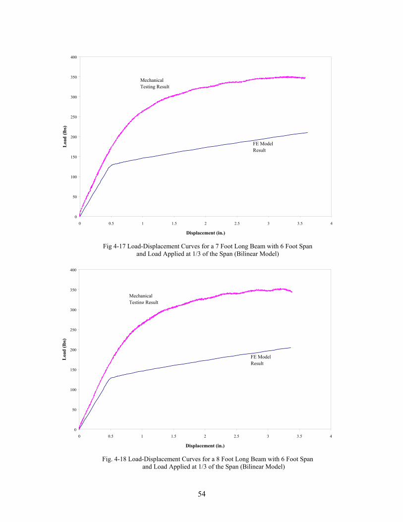
The load-displacement curves generated by the hyperfoam and bilinear models and
the curves obtained from beam bending testing did not match. However, the hyperbolic
tangent model matched the data quite well.
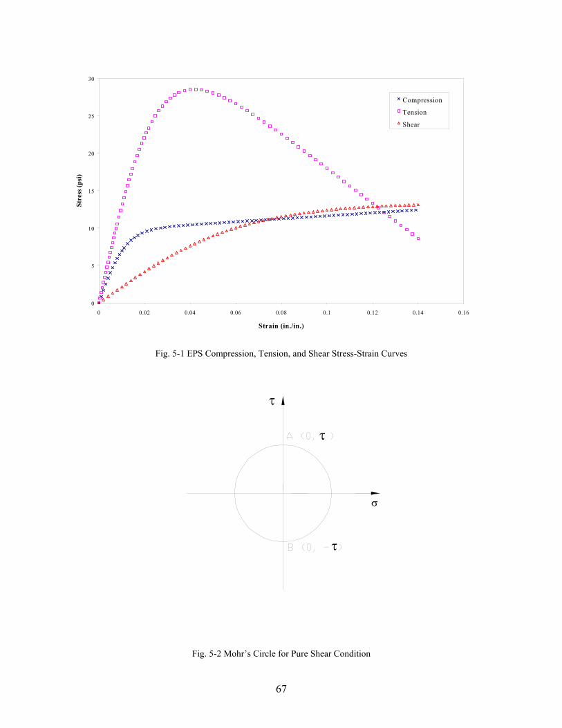
Both experimental data and analytical modeling showed that the SIPs behavior is
governed by compression and shear of EPS. A multi-span flexure test can be used to obtain
an initial shear modulus and compression strength can be used as the shear strength. Future
design equations for SIPs must incorporate checks for shear and bearing capacity.
vi
TABLE OF CONTENTS
Acknowledgement………………………………………………………………. iii
Abstract……………………………………………………………………………. iv
Table of Contents……………………………………………………………….. vi
List of Figures……………………………………………………………………. viii
List of Tables……………………………………………………………………... x
Chapter 1: Introduction Statement of Problem………………………………………………………… 1 Research Objective…………………………………………………………… 3
Chapter 2: Literature Review
ICBO ES………………………………………………………………………. 5 APA-Design Specifications………………………………………………… 5 Esvelt’s Research……………………………………………………………... 7 Noor, Burton, and Bert’s Review………………………………………….. 8 Frostig’s High-Order Theories……………………………………………... 9 Bozo’s Results………………………………………………………………… 11 Rusmee and DeVries’s Research on EPS Foam………………………… 11 Published Mechanical Properties for EPS……………………………….. 12 Hyperbolic and Linear Function…………………………………………… 13
Chapter 3: Research Methods
Mechanical Testing…………………………………………………………... 17 EPS Compression Test………………………………………………………... 17 EPS Tension Test……………………………………………………………... 18 EPS Shear Test………………………………………………………………... 19 SIP Flexural Test……………………………………………………………… 20 EPS Density Test……………………………………………………………… 23 Finite Element Methods…………………………………………………….. 23 Hyperfoam Model for EPS Core……………………………………………… 23 Uniaxial Compression Mode……………………………………………….. 24 Simple Shear Mode…………………………………………………………. 24 Bilinear Model for EPS Core…………………………………………………... 25
vii
User-Supplied Model for EPS Core……………………………………………. 25 Finite Element Model for a SIP Beam…………………………………………. 26
Chapter 4: Research Results
Mechanical Testing Results………………………………………………….. 38 EPS Compression Test Results………………………………………………… 38 Discontinuity Point…………………………………………………………... 38 EPS Tension Test Results……………………………………………………… 39 Discontinuity Point…………………………………………………………... 39 EPS Shear Test Results………………………………………………………… 40 EPS Bending Test Results……………………………………………………… 40 Constants c1 to c3 and Initial Slope of SIP Beams…………………………... 40 Shear Modulus in Flexure…………………………………………………… 41 EPS Density……………………………………………………………………. 42 Finite Element Results………………………………………………………... 42 Hyperfoam Model for EPS Core……………………………………………….. 42 Uniaxial Compression Mode………………………………………………… 42 Simple Shear Mode…………………………………………………………... 43 Bilinear Model for EPS Core………………………………………….……….. 43 User-Supplied Model for EPS Core……………………………………………. 43 User-Supplied Material 1……………………………………………………. 44 User-Supplied Material 2……………………………………………………. 44
Chapter 5: Discussion and Conclusions
Discussion……………………………………………………………………… 61 Material Properties…………………………………………………………….. 61 Stress-Strain Curves…………………………………………………………… 62 Design Point…………………………………………………………………… 63 Conclusions……………………………………………………………………. 64 References………………………………………………………………………… 71
Appendix A The Uniaxial Compression Mode of the Hyperfoam Model………… 74
Appendix B The Simple Shear Mode of the Hyperfoam Model……………………. 78
viii
LIST Of FIGURES
Figure 2-1 : Dimensions of Structural Sandwich Panel Used in the APA’s Design Equation……………………………………………………………….. 14 Figure 2-2 : Geometry, Load, Internal Results and Deformation………………….. 15 Figure 2-3 : Hyperbolic and Linear Function……………………………………… 16 Figure 3-1 : Dimensions of Structural Insulated Panel…………………………….. 27 Figure 3-2 : Dimensions of Compression Sample…………………………………. 28 Figure 3-3 : Compression Test Set-up……………………………………………... 29 Figure 3-4 : Dimensions of Tension Sample………………………………………. 30 Figure 3-5 : Tension Test Set-up…………………………………………………... 31 Figure 3-6 : Dimensions of Shear Sample…………………………………………. 32 Figure 3-7 : Shear Test Set-up……………………………………………………... 33 Figure 3-8 : Dimensions of SIPs Flexural Test…………………………………….. 34 Figure 3-9 : Dimensions of SIP Beam’s Cross Section……………………………. 35 Figure 3-10: Idealized Stress-Strain Curve for Bilinear Material………………….. 36 Figure 3-11: Typical Model for SIP Beams………………………………………… 37 Figure 4-1 : Stress-Strain Curves for EPS in Compression………………………... 46 Figure 4-2 : Stress-Strain Curves for EPS in Compression between Testing & Hyperbolic and linear Function Fit…………………………………… 46 Figure 4-3 : EPS Continuous Point for Compression……………………………… 47 Figure 4-4 : Stress-Strain Curves for EPS in Tension…………………………….. 47 Figure 4-5 : Stress-Strain Curves for EPS in Tension between Testing & Hyperbolic and Linear Function Fit………………………………….. 48 Figure 4-6 : EPS Discontinuous Point for Tension………………………………… 48 Figure 4-7 : Stress-Strain Curves for EPS in Shear……………………………….. 49 Figure 4-8 : Stress-Strain Curves for EPS in Shear between Testing & Hyperbolic and Linear Function Fit………………………………….. 49 Figure 4-9 : Load-Displacement Curves for SIP Beam at Various Span………….. 50 Figure 4-10: Determination of the Slope by Plotting Initial Slopes of the Load-Displacement Curves…………………………………………… 50 Figure 4-11 : Comparison of Strain-Stress Curves from Compression Test and Uniaxial Compression Mode of Hyperfoam Model………………….
51
Figure 4-12: Comparison of Strain-Stress Curves from Shear Test and Simple Shear Mode of Hyperfoam Model……………………………………. 51 Figure 4-13: Comparison of Load-Displacement Curves of EPS in Compression from Mechanical Test and Bilinear Model…………………………... 52 Figure 4-14: Comparison of Load-Displacement Curves of EPS in Tension from Mechanical Test and Bilinear Model………………………….……… 52 Figure 4-15: Load-Displacement Curves for a 3 Foot Long Beam with 2 Foot Span and Load Applied at 1/3 of the Span (Bilinear Model)……………….
53
Figure 4-16: Load-Displacement Curves for a 5 Foot Long Beam with 4 Foot Span and Load Applied at 1/3 of the Span (Bilinear Model)………………..
53
Figure 4-17: Load-Displacement Curves for a 7 Foot Long Beam with 6 Foot Span and Load Applied at 1/3 of the Span (Bilinear Model)……………….
54
ix
Figure 4-18: Load-Displacement Curves for an 8 Foot Long Beam with 6 Foot Span and Load Applied at 1/3 of the Span (Bilinear Model)……………….
54
Figure 4-19: Load-Displacement Curves for an 8 Foot Long Beam with 8 Foot Span and Load Applied at 1/3 of the Span (Bilinear Model)……………….
55
Figure 4-20: Load-Displacement Curves for a 3 Foot Long Beam with 2 Foot Span and Load Applied at 1/3 of the Span (User-Supplied Input 1)……….
55
Figure 4-21: Load-Displacement Curves for a 5 Foot Long Beam with 4 Foot Span and Load Applied at 1/3 of the Span (User-Supplied Input 1)………..
56
Figure 4-22: Load-Displacement Curves for a 7 Foot Long Beam with 6 Foot Span and Load Applied at 1/3 of the Span (User-Supplied Input 1)……….
56
Figure 4-23: Load-Displacement Curves for an 8 Foot Long Beam 6 Foot Span and Load Applied at 1/3 of the Span (User-Supplied Input 1)……….
57
Figure 4-24: Load-Displacement Curves for an 8 Foot Long Beam with 8 Foot Span and Load Applied at 1/3 of the Span (User-Supplied Input 1)……….
57
Figure 4-25: Load-Displacement Curves for a 3 Foot Long Beam with 2 Foot Span and Load Applied at 1/3 of the Span (User-Supplied Input 2)……….
58
Figure 4-26: Load-Displacement Curves for a 5 Foot Long Beam with 4 Foot Span and Load Applied at 1/3 of the Span (User-Supplied Input 2)………..
58
Figure 4-27: Load-Displacement Curves for a 7 Foot Long Beam with 6 Foot Span and Load Applied at 1/3 of the Span (User-Supplied Input 2)………..
59
Figure 4-28: Load-Displacement Curves for an 8 Foot Long Beam with 6 Foot Span and Load Applied at 1/3 of the Span (User-Supplied Input 2)………..
59
Figure 4-29: Load-Displacement Curves for an 8 Foot Long Beam with 8 Foot Span and Load Applied at 1/3 of the Span (User-Supplied Input 2)………..
60
Figure 5-1 : EPS Compression, Tension, and Shear Stress-Strain Curves……….... 67 Figure 5-2 : Mohr’s Circle for Pure Shear Condition…………………………….... 67 Figure 5-3 : Comparison of Load-Displacement Curves with Different Input for Tension Properties………………………………………………….…
68
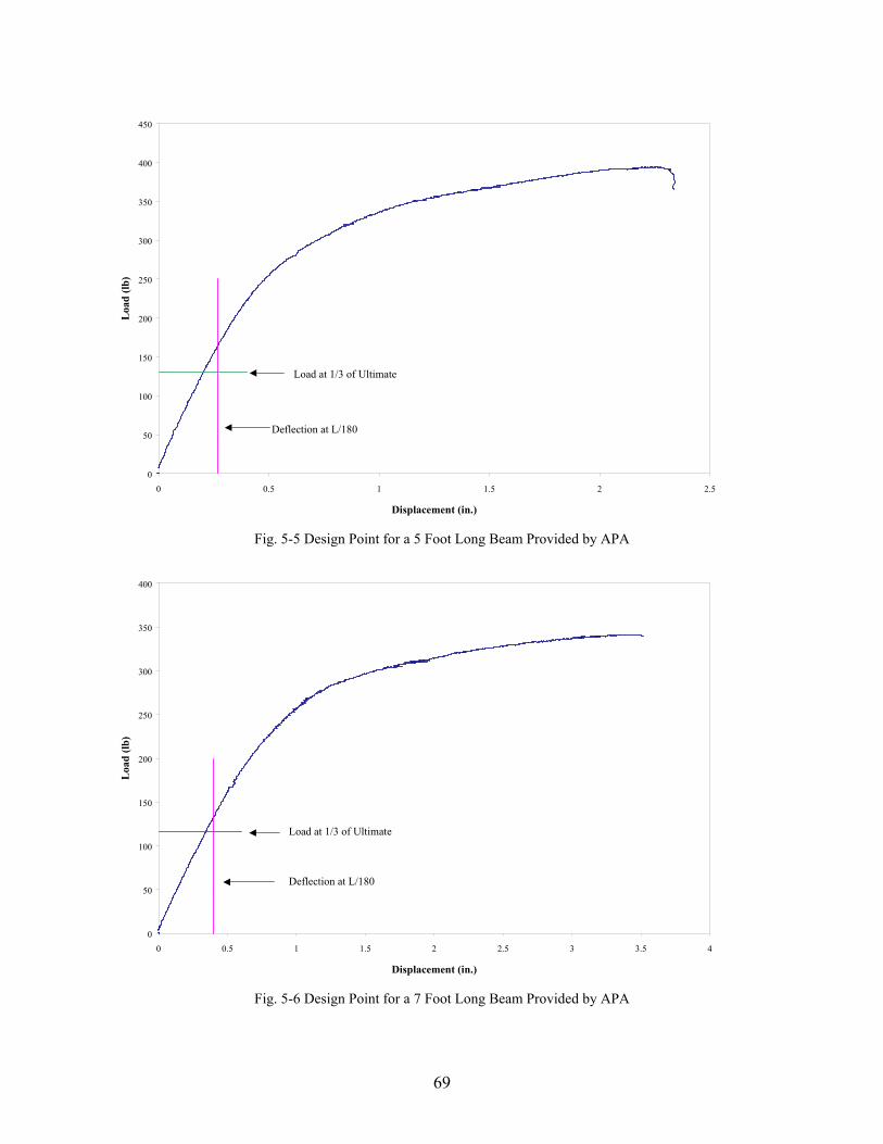
Figure 5-4 : Design Point for a 3 Feet Beam Provided by APA………………….... 68 Figure 5-5 : Design Point for a 5 Feet Beam Provided by APA………………….... 69 Figure 5-6 : Design Point for a 7 Feet Beam Provided by APA………………….... 69 Figure 5-7 : Design Point for an 8 Feet Beam Provided by APA…………………. 70
x
LIST Of TABLES
Table 2-1: OSB Mechanical Properties with a Nominal Density of 650 Kg/m3………………………………………………………….. 11 Table 2-2: EPS Properties Published by ASTM Standard…………………….. 12 Table 2-3: EPS Properties Published by Huntsman Corporation……………… 12 Table 3-1: SIP Block Dimensions for Compression Tests…………………….. 18 Table 3-2: SIP Block Dimensions for Tension Tests………………………….. 18 Table 3-3: SIP Block Dimensions for Shear Tests…………………………….. 19 Table 3-4: Set-up Dimensions and Test Speed for Beam Bending Testing…… 20 Table 3-5: EPS Dimensions for Density Tests………………………………… 23 Table 4-1: Constants c1 to c3 Values and Initial Slope for Beams…………….. 41 Table 4-2: Values of x-y for Calculating EPS Shear Modulus………………... 41 Table 4-3: EPS Density in This Research……………………………………... 42 Table 4-4: Inputs of User-Supplied Material 1 for EPS……………………….. 44 Table 4-5: Inputs of User-Supplied Material 2 for EPS……………………….. 45 Table 5-1: Published by ASTM and Calculated Values of EPS Compression Properties…….……………………………………………………..
61
Table 5-2: Published by Huntsman Corporation and Calculated Values of EPS Compression Properties…….……………………………………….
61
Table 5-3: Comparison of APA Predicted Values and Testing Results at 1/3 of Max Load and Deflection at L/180 Situations…………………... 65 Table 5-4: Comparison of APA Predicted Values and Testing Results at Max Load Situation……………………………………………….…….. 66
1
Chapter 1
INTRODUCTION
Structural insulated panels (SIPs) are a sandwich system constructed with an insulating core
between two structural sheathings. They can be used in walls, roofing, and flooring. The core
provides insulation and shear rigidity, and sheathings provide flexural stiffness and durability.
Expanded polystyrene (EPS), extruded polystyrene (XPS), and polyurethane are the most common
core materials. Sheathings typically are made of oriented strand board (OSB) or plywood. The
research reported here focuses on SIPs that consist of OSB sheathings and EPS core since they are
the most commonly used in residential applications.
STATEMENT OF PROBLEM
The use of structural insulated panel in residential building began in the 1950s. Since then, SIP
manufacturers have continued to develop the manufacturing process and the product [1].
Fluctuating lumber prices, lumber quality, greater concern for energy conservation, ease of
construction, and economy have encouraged greater SIP use over the last two decades.
The International Conference of Building Officials Evaluation Service, Inc. (ICBO ES)
does technical evaluations of building products, components, methods, and materials. ICBO ES
acceptance criteria are documents for evaluating a type of product, and establishing conditions of
acceptance. Acceptance Criteria for Sandwich Panels AC04 [2] provides a guideline for
recognition of sandwich panels under the Uniform Building Code (UBC), the International
Building Code (IBC), and the International Residential Code (IRC). The criteria require that full-
scale panels be tested for their specific use. Allowable loads may be interpolated for smaller scale
panels, but extrapolation to larger panels is not permitted. Obviously, it is expensive and time
2
consuming to test large panels. The criteria also permit the use of rational analysis to obtain
mechanical properties of full-scale panel based on each component’s mechanical properties.
APA-The Engineered Wood Association (APA) published the design specifications for
plywood sandwich panels [3]. Those equations in the APA publication are based upon classical
laminated beam theory that only includes a deflection check and stress checks due to bending and
shear. Esvelt [4] conducted laboratory tests of full-size panels in 1999 and found that the SIPs
failed either in shear at a wire chase or bearing at a support, with one exception in bending. Yet,
the published APA design equations do not include bearing checks, nor predict the correct
deflections. The APA calculations deflections differed by 2 to 12 standard deviations from those
observed in Esvelt’s testing. Esvelt concluded from her research that the APA’s design equations
are inaccurate and incomplete.
Many computational models based on rational analysis have been developed for predicting
the response of sandwich panels [5]. However most have been developed only to model sandwich
panels with metal honeycomb core and metal or synthetic composite sheathing in aeronautical
applications. Expanded polystyrene (EPS) has very different mechanical properties than metal
honeycomb. The applicability of these computational models for sandwich panels is critically
dependent on the core’s properties. To date, no reliable computational models have been
developed for SIPs with OSB sheathing and EPS core.
Classical beam theories assume that there is no transverse flexibility of the core.
Obviously, the assumption is not applicable for SIPs, for which deflection of the top and bottom
sheathings are not equal due to deformation of the compressible core. Frostig et al. [6] used high-
order theories in the analysis of sandwich beams with a transversely flexural core, ie, through the
depth of the beam. High-order theories include the non-linearity of the longitudinal and the
3
transverse deformations of the core through the depth and incorporate appropriate boundary
conditions at the interface between core and sheathing. They can be used in analyzing SIPs that
consist of various sheathing material and dimensions and core material of foam or honeycomb.
These theories are applicable to all types of loading and boundary conditions [6, 7].
High-order theories proved to be a more accurate predictor of a composite beam’s
mechanical response to loading, but their use is far too complicated for a design equation. Accurate
and simplified design equations for SIPs are needed. An understanding of the behavior of SIPs
under transverse loading is prerequisite to generating those simplified design equations.
OBJECTIVES
The hypothesis for this research is that the mechanical response of SIPs in flexure can be predicted
from the mechanical responses of the individual components. The research objective for the work
described here is to obtain the mechanical response of the individual components, EPS foam and
OSB sheathing, and of the flexure response of SIP beams and to use these responses to model,
within finite element analysis, the response of the observed SIP. Such a model would help to
identify the critical point and failure mode in SIPs which can lead to future research to developing
simplified design equations.
4
Chapter 2
LITERATURE REVIEW
The International Conference of Building Officials Evaluation Service, Inc. (ICBO ES), does
technical evaluations of building products, components, methods, and materials. ICBO ES
provides “Acceptance Criteria for Sandwich Panels AC04” [2] for sandwich panels’ evaluation.
The criteria require that full-scale panels be tested for their specific use. Allowable loads may
be interpolated for smaller scale panels, but extrapolation to larger is not permitted. However, the
criteria also allow the use of rational analysis to obtain mechanical properties for full-scale panels
based on each component’s properties. APA published the design specifications for plywood
sandwich panels according to classical beam theory [3]. However, Esvelt found that the APA
design specifications can not accurately predict SIPs’ behavior [4]. Noor, Burton, and Bert have
published a literature review of computational models for sandwich panels and plates [5]. Included
among their more than 800 references is Frostig’s “High-Order Theory in Analysis of Sandwich
Beams with a Transversely Flexural Core” [6].
ABAQUS and ADINA are two finite element analysis programs that can be used for
computational analysis of SIPs. Mechanical properties of OSB sheathings and EPS core are
required inputs. For the OSB sheathing, necessary properties were provided by Bozo [8].
However, there are some difficulties in determining the mechanical properties of EPS foam [9].
EPS mechanical properties have been published by ASTM [10] and they appear on some EPS
industry websites [11]. But those were limited to a single value of material properties. For
ADINA’s user-supplied material, a stress-strain curve is required to describe every material
property. Murphy found that a hyperbolic and linear equation can fit stress-strain data of
5
woodfiber-plastic composites with four parameters [12].
ICBO ES
The ICBO ES oversees technical evaluations of building products, components, methods, and
materials. In July 2001, they issued “Acceptance Criteria for Sandwich Panels[2].” The criteria,
which is consistent with Uniform Building Code, International Building Code, and International
Residential Code, provides a procedure for recognition of sandwich panels.
The criteria stipulate that full-scale panel tests must be performed to determine the
allowable load. This may be interpolated for smaller scale panels, but extrapolation to larger ones
is not permitted. According to panels’ usage and load type, the following tests may need to be
conducted: wall panels transverse load test, wall panels axial load test, wall panels racking shear
tests, roof and floor panels uniform load test, and roof and floor concentrated load test. Three tests
of each type are mandated with the results varying no more than 15 percent from the average of
the three. A minimum factor of safety of three is applicable to the ultimate load according to the
average test value. When tests are not conducted to failure, the highest load reached for each test
will be assumed to be ultimate.
To provide flexibility of panel size, the criteria permit the use of rational analysis to obtain
full-scale panels’ mechanical properties based on each component’s properties. Confirmatory
tests on actual panels will only be necessary for verifying design assumptions and criteria.
APA’S DESIGN SPECIFICATIONS
APA-The Engineered Wood Association published “Design and Fabrication of Plywood Sandwich
Panels” [3] based on rational analysis. This publication presents a method for design of sandwich
panels under horizontal, vertical, or combined loading. It is assumed that a sandwich panel acts
6
as a laminated beam. Axial forces and bending moments are resisted by the sheathings, shear
forces and stability of the sheathings are carried by the core.
The dimensions of a structural sandwich panel used in the APA specifications are shown
in Figure 2-1. Deflection and stresses for structural sandwich panels in these specifications are
found as:
(1) Deflection due to uniform transverse loading only is
c
sb GchwL
EIwL
)(438417285 24
++
×=∆+∆=∆ (1)
Total deflection including the effects of axial loads is approximately equal to
crPP /1max −
∆=∆ (2)
( )
( ) ( )
+×+
=
c
cr
GchLEIL
EIP
612112 2
22
2
π
π (3)
(2) Maximum bending stress
1
max2
max,5.1
SPwL
fb∆+
= (4)
(3) Maximum shear stress
)(12 chwLfv +
= (5)
Where,
A1 = area of upper sheathing (in.2/ft) A2 = area of lower sheathing (in.2/ft) c = core thickness (in.) h = panel thickness (in.) E = modulus of elasticity of plywood (psi) Gc = modulus of rigidity of core (shear modulus) in direction of span (psi) I = panel moment of inertia (in.4 per foot of width)
7
L = span length (ft) P = axial load (lb per foot of panel width) Pcr = theoretical column buckling load (lb per foot of panel width) S = section modulus of panel (in.3 per foot of width) S1 = section modulus with A1 face in tension S2 = section modulus with A2 face in tension w = normal uniform load (psf) y = distance from neutral axis to outmost fiber (in.) ∆ = deflection due to transverse loading (in.) ∆b = deflection due to bending (in.) ∆s = deflection due to shear (in.)
)(4)(
21
221
AAchAA
I++
= (6)
y
Syh
S 1,121 =
−= (7)
21
22
11 )
2()
2(
AA
tA
thA
y+
+−= (8)
ESVELT’S RESEARCH
Esvelt [4] investigated the behavior of structural insulated panels under transverse loading. She
determined the core and sheathing mechanical properties and modeled panels under various
failure modes. In the initial step, Esvelt performed small-size testing of the EPS core in tension,
compression, and shear. The modulus of elasticity, yield stress, maximum strength and strain-
stress curve also were obtained from small-size testing of OSB sheathing in bending.
Additionally, Esvelt tested full-scale panels with simple-span and multi-span under a uniform
transverse load. Two common failure modes (shear failure for panel with wire chase and bearing
failure for panel without wire chase), and one uncommon failure (flexural failure) were observed
during testing. Loads that produced the mid-span deflection of L/360, L/240, and L/180 were
8
recorded. Empirical data and calculated data obtained from the APA design equations then were
compared. The APA design equation significantly under-predicted the actual load to deflect the
panels at L/360, L/240, and L/180 by between 2 and 12 standard deviations.
Esvelt used the COSMOS finite element program for modeling SIPs. A plane strain, two-
dimensional, four-node isoparametric element was used to analyze SIPs’ non-linear behavior. For
deflection models, the differences between the finite element model and laboratory results ranged
from -5.6% to 31.1%, which showed that these models failed to predict panels’ actual response.
For the bearing failure model, she suggested modeling the core as a bilinear material. She
determined that even a minor change of the core’s shear modulus significantly affected the
stiffness of SIPs.
NOOR, BURTON, AND BERT’S REVIEW
Noor, Burton, and Bert [5] performed an extensive literature review of sandwich panels. In that
review, they classified the various computational models for predicting the response of sandwich
panels and shells as ordinary, open-face, and multi-layer. The modeling method distinguished four
categories: detailed models, three-dimensional continuum models, two-dimensional plate and
shell models, and simplified models. Most studies they referenced focused on metallic and
nonmetallic honeycomb cores. Knowing core properties is a prerequisite for modeling sandwich
panels and shells with reliable response predictions. They grouped their citations on core
properties’ determination in three categories: experiments, analytical models, and finite element
models.
The authors also reviewed the literature on miscellaneous problems of sandwich panels
and shells. These were listed under ten categories: heat transfer; static thermomechanical stress;
free vibrations and damping; transient dynamic response; bifurcation buckling, local buckling,
9
face sheet wrinkling and core crimping; large deflection and post-buckling; effects of
discontinuities and geometric changes; damage and failure of sandwich structures; experimental
studies; and optimization and design studies.
In the thermomechanical stress analysis category, research has been performed in three
general geometries: panels with rectangular cross-section, panels with circular cross-section, and
cylindrical shells with circular cross-section.
FROSTIG’S HIGH-ORDER THEORY
Frostig, et al [6] pioneered the use of high-order theory in the analysis of sandwich beams with a
transversely flexural core. The theory assumes sheathings to be ordinary thin beams, acting
only longitudinally, and interconnected through equilibrium and compatibility at their interface
with the core. The core is considered to be a two-dimensional elastic medium. All behavior
equations, with given boundary and continuity conditions, for the entire beam can be derived from
the horizontal and vertical deflections of the upper and lower sheathings and the shear stress in
the core.
This high-order theory is based on the following four assumptions: 1) longitudinal
stresses in the core are negligible; 2) height of the core and its plane section can deform in a
nonlinear pattern; 3) stresses and deformation fields are uniform through the width; and 4) loads
applied at the sheathings can be arbitrary. Figure 2-2 provides the information necessary to
analyze sandwich panels using high-order theory.
The governing equations are:
txxott nbuEA −=+τ, (9)
10
bxxobb nbuEA −=+τ, (10)
xtttxbctc
xxxxtt mqdcb
cwbE
cwbE
wEI ,,
, 2)(
−=+
−−+τ
(11)
xbbbxbctc
xxxxbb mqdcb
cwbE
cwbE
wEI ,,
, 2)(
−=+
−+−τ
(12)
0122
)(2
)( ,,, =+−+
−+
−−cc
xxbxbtxtobot G
bcEbcdcbwdcbw
bubu ττ (13)
Where,
tEA = axial rigidities of top sheathing
bEA = axial rigidities of bottom sheathing
otu = longitudinal displacement of centroid of the top sheathing
obu = longitudinal displacement of centroid of the bottom sheathing τ = shear stress in core b = width of beam
tn = distributed horizontal stress resulted from external loads in top sheathing
bn = distributed horizontal stress resulted from external loads in bottom sheathing
tEI = flexural rigidities of top sheathing
bEI = flexural rigidities of top sheathing
tw = vertical displacement of centroid of top sheathing
bw = vertical displacement of centroid of bottom sheathing
cE = elastic modulus of core c = height of core
td = thickness of top sheathing
bd = thickness of bottom sheathing
tq = distributed vertical stress resulted from external loads in top sheathing
bq = the distributed vertical stress resulted from external loads in bottom sheathing
tm = bending moments resulted from external load in top sheathing
bm = bending moments resulted from external load in bottom sheathing
cG = shear modulus of core
The order of the equivalent differential equation that replaces this set of equations (9) to
(13) is 14. Under certain boundary conditions, those five equations above can be solved for
11
vertical and horizontal displacements in the top and bottom sheathings, and shear stress in the core.
The normal stresses at the upper sheathing and lower sheathing are shown in Eq. (14) and (15).
2)(
)0,( , cc
wwEzx xtbc
zz
τσ +
−== (14)
2)(
),( , cc
wwEczx xtbc
zz
τσ −
−== (15)
BOZO’S RESULTS
Bozo [8] conducted mechanical testing of OSB with three different nominal densities of 450 kg/m3,
550 kg/m3, and 650 kg/m3, respectively, with tolerance limit of ± 25 kg/m3. The mechanical
properties studied in his research were the modulus of elasticity and maximum values for
compression, tension, and shear. Compression and tension tests were performed according to
ASTM D1037. Shear tests were conducted based on ASTM D5379/D5379M-93. The crosshead
displacement speed in his tension tests was controlled to be 4.0 mm/minute, while in compression
and shear tests, the speed was 0.36 mm/minute. Mechanical properties for OSB with a density of
650 kg/m3 are shown in Table 2-1.
OSB Max Stress (Psi) E or G (Psi) Compression (E) 1700 594000
Tension (E) 1800 790000 Shear (G) 1330 200000
Table 2-1 OSB Mechanical Properties with a Nominal Density of 650 Kg/m3
RUSMEE AND DEVRIES’ RESEARCH ON EPS FOAM
P. Rusmee and K. L. DeVries[9]’ research showed that the size, loading rate, and loading
configuration have significant influences on the apparent material properties of EPS foam. From
three groups of mechanical tests of EPS with different size, loading rate, and loading
configuration, they found that the modulus in compression they obtained from the 13 mm thick
12
foam specimens was 0.9 MPa and 2.8 MPa for 50 mm thick foam. The modulus for the 50 mm
thick foam increased to 3.3 MPa as the loading rate increased from 0.042 mm/s to 4.2 mm/s. In
a dynamic test, the value of the modulus for 50.8 mm thick foam was about 390% of the value of
the quasi-static modulus. They drew the conclusion that when using EPS foam in design, one
needs to determine the usage condition, such as its lateral dimensions, thickness, and rate of
loading.
PUBLISHED MECHANICAL PROPERTIES FOR EPS
ASTM C578 Standard Specifications for Rigid, Cellular Polystyrene Thermal Insulation [10]
provides the EPS physical property requirements of thermal insulation based on EPS type. The
strength properties for EPS are shown in Table 2-2.
EPS Type Properties
Type I Type VIII Type II Type VI
Density, minimum (pcf) 0.90 1.15 1.35 1.80
Compressive 10% Deformation (psi) 10 13 15 25
Table 2-2 EPS Properties Published by ASTM Standard
For other material characteristics that are not required by the standards, but are very
important, were modified by the Huntsman Corporation [11]. Their modified EPS typical
physical properties at 1 lb/ft3 is listed in Table 2-3.
Property Value
Tensile Strength (psi) 28
Shear Strength (psi) 16
Shear Modulus (psi) 440
Table 2-3 EPS Properties Published by Huntsman Corporation
13
HYPERBOLIC AND LINEAR FUNCTION
Nonlinear materials, such as woodfiber-plastic composites, behave differently compared to wood
and wood products. The Engineering Mechanics Laboratory of the USDA Forest Service
generated a four parameter hyperbolic and linear function to fit load-displacement data for paper,
joint slip, steel, and woodfiber-plastic composites. Using these four known parameters, one can
determine the theoretical load-displacement curve as well as its initial slope.
The hyperbolic and linear function is
)())(( 43421 cxccxcTanhcp −+−= (16)
and the slope at x is
3422
21 ))(( ccxcSechccdxdp
+−= (17)
The initial slope at x = zero is
321 cccdxdp
+= (18)
The parameters are estimated using standard nonlinear least-squares techniques. The
intercept of the curve at the x-axis is c4, and the slope of the second straight line is c3 as shown in
Figure 2-3.
15
Fig. 2-2 Geometry, Load, Internal Results and Deformation: (a) geometry; (b) internal Resultants and stresses; (c) external loads; (d) deformation pattern
τ τ τ
τ
τ σ
σ
17
Chapter 3
RESEARCH METHODS Modeling of SIPs was accomplished in three steps. First, the mechanical properties of panel
components, OSB sheathing and EPS core were collected. Compression, tension, and shear
properties of OSB sheathing were obtained from Bozo [8]. The compression, tension, and shear
properties of the EPS core were obtained from mechanical testing as described below. Also, EPS
density in this research was determined for the comparison of shear modulus between calculated
and published values [10]. Second, the material properties obtained from above were used with
three different material models within finite element programs. Lastly, sections of SIP panels
were tested in flexure to validate the finite element analysis.
MECHANICAL TESTING
Four structural insulated panels used in this research were obtained from R-Control Group of
Excelsior, MN. Each of the four panels measured 4 ft by 8 ft. OSB sheathing had a thickness of
7/16 in. and the EPS core had a thickness of 3-5/8 in. as shown in Figure 3-1. Using a band saw,
SIPs were cut into 3.5 in. wide beams for flexural testing. Left-over ends from cutting beams were
used for compression, tension, and shear specimens.
EPS COMPRESSION TESTS
Compression testing specimens were fabricated from SIP strip ends as shown in Figure 3-2. First,
two-inch-wide specimens were cut from the edge of left-over SIP ends. Then they were cut to
make 2.00 in. by 2.00 in. by 4.50 in. blocks. Seven of these blocks were used for testing.
Specimen dimensions are listed in Table 3-1.
18
Compression Width (in.) Thickness (in.) C1 2.05 1.97 C2 2.05 1.99 C3 2.05 2.01 C4 2.08 1.99 C5 2.05 2.03 C6 2.07 2.00 C7 2.06 2.02
Table 3-1 SIP Block Dimensions for Compression Tests
The compression test setup is shown in Figure 3-3. Specimens were tested at a speed of
0.15 in./min. with an Instron universal test machine (model number: 4466) having a load range
of ± 2 kips. A 1-inch MTS extensometer (Model number: 634.12E-24) with strain range from
–10% to + 50% was centered midway on the EPS core height. The EPS foam was wrapped with
thick paper to eliminate the damage resulting from fastening the extensometer. Data was collected
at 2 samples per second.
EPS TENSION TESTS
Fabrication of tension testing specimens followed the same procedures used to make those for
compression, but with cross-section of 1.80 in. by 2.00 in. as shown in Figure 3-4. Blocks then
were refined to dog-bone shape. Dimensions of the dog-bone cross-section for each specimen are
listed in Table 3-2.
Tension Width (in.) Thickness (in.) T1 1.80 1.06 T2 1.83 1.12 T3 1.79 1.12 T4 1.82 1.10 T5 1.79 1.05 T6 1.84 1.08 T7 1.80 1.10
Table 3-2 SIP Block Dimensions for Tension Tests
Tension tests were performed as shown in Figure 3-5. They were tested at a speed of
19
0.05 in./min. with an Instron universal test machine (model number: 4466) having a load range of
± 2 kips. A 1-inch MTS extensometer (model number: 634.12E-24) with strain range from –10%
to +50% was centered midway on the EPS core height. Again, the EPS foam was wrapped with
thick paper to eliminate the damage resulted from fastening the extensometer. Data was collected
at 2 samples per second.
EPS SHEAR TESTS
Shear testing specimens were cut as shown in Figure 3-6. Top and bottom OSB sheathings were
originally attached to EPS 1 and 2, which were glued to OSB 1. In order to ensure that top and
bottom OSB sheathings remain vertical when applying load to OSB 1, using Arrow hot melt glue,
OSB 2 and OSB 3 were glued to both ends of top and bottom OSB sheathings. OSB 4 was then
glued to top and bottom OSB sheathings. Sixteen 1.00 in. by 2.00 in. by 3.00 in. EPS blocks were
glued to eight specimens. EPS shear dimensions are listed in Table 3-3.
Shear Length (in.) Thickness (in.) S1 2.99 2.03 S2 3.02 2.04 S3 2.98 2.03 S4 3.00 2.05 S5 2.97 1.98 S6 2.98 1.97 S7 2.48 2.04 S8 2.47 1.97
Table 3-3 SIP Block Dimensions for Shear Tests
The shear test setup is as shown in Figure 3-7. They were tested at a speed of 0.02 in./min.
with an Instron (model number: 4466) having a load range between ± 2 kips. A 1-inch MTS
Extensometer (model number: 634.12E-24) with strain range from –10% to + 50% was centered
midway on the left side of the EPS core. Data were collected at either 2 samples or 5 samples per
second.
20
SIPS FLEXURAL TEST
Structural insulated panels were cut into 3.5 in. wide beams with lengths of 3 feet, 5 feet,
7 feet, and 8 feet. Beams were tested in five groups: 1) 3 foot long beam with 2 foot span; 2) 5
foot long beam with 4 foot span; 3) 7 foot long beam with 6 foot span; 4) 8 foot long beam with
6 foot span; and 5) 8 foot long beam with 8 foot span. Three beams were tested in groups 1 to 3
and one beam in groups 4 and 5. Each beam was subjected to concentrated loads at the third-
points. They were tested with an Instron machine (model number: 1137) of load range between
±30 kips. A linear varying differential transducer with a range of ± 2 in. was used to determine
the deflection of SIP beams at the mid-span. Data was collected at 5 points per second. The
flexural test setup is shown in Figure 3-8.
Detailed set-up dimensions and test speed for each group are listed in Table 3-4.
Group Distance a (in.) Distance L (in.) Test Speed (in./min.)
1 6 24 0.15 2 6 48 0.20 3 6 72 0.20 4 12 72 0.30 5 0 96 0.30
Table 3-4 Set-up Dimensions and Test Speed for Beam Bending Testing
SHEAR MODULUS VIA FLEXURAL TEST
ASTM D 198 [13] provides a formula for calculating shear modulus via flexural test. The
elastic deflection of a prismatic beam under a single center point load is:
'
3
448 GAPL
EIPL
+=∆ (19)
where,
∆------deflection at mid-span, P------applied load, L------span,
21
E------modulus of elasticity, I-------moment of inertia,
G-------shear modulus, A’------modified shear area.
If the shear contribution is ignored, the relationship between deflection and “apparent”
modulus of elasticity (Ef) is:
IEPL
f48
3
=∆ (20)
Eq. (19) then can be rewritten as Eq. (21)
2)/(111 LhKGEE f
+= (21)
Where,
νν
1112)1(10
++
=K for rectangular cross-section
( )νν
6716++
=K for circular cross-section
ν is Poisson’s ration.
For each beam span, the “apparent” modulus of elasticity (Ef) can be calculated using
Eq. (20). Plotting 1/Ef versus (h/L)2 for each span produces a distribution of points that can be
approximated by a straight line. Knowing the slope k of that line, shear modulus kK
G 1= .
For a simply supported beam under double quarter-point loads, the deflection due to
bending is EI
PL129623 3
1 =∆ , and the deflection due to shear is AGM
=∆ 2 [14],
Where,
P = load applied at the beam,
A = bh2/c (for sandwich beams),
22
M = the moment at mid-pan.
Dimensions of the SIP beam’s cross section is shown in Figure 3-9.
For a SIP beam,
1226
321
21 bcEhbcEbcEEI css ++= (22)
If 10032
1
>
ch , then the first term of Eq. (22) can be ignored,
and if ,10062
1 >
ch
cc
EE
c
s then the third term in Eq. (22) can be ignored.
For the SIP beams used in this research, 1002594375.00625.433
22
1
>=
=
ch , and
,100487625.30625.4
625.34375.0
85445687666
221 >=
=
ch
cc
EE
c
s
So, Eq. (22) can be simplified as
2
21hbcEEI s= (23)
Eq. (19) can be rewritten again as
GbhPLc
EhbcPL
GbhPLc
hbcE
PL
s
s
221
3
221
3
664823
62
1296
23
+=
+=∆
(24)
Also,
( ) fsEhbcPL
21
3
64823
=∆ (25)
Eq. (24) can be written as
23
( )
21
21
123
1081
123
10811
LGcc
E
Lcc
GEE
cs
csfs
+=
+=
(26)
To remove the foam’s crushing from the determination, (Es)f was calculated according to
the initial slope of the load-displacement curve of SIP beams bending. Equation (26) can be
graphed as a line by letting y = 1/ (Es)f and x = (1/L)2. In the resulting graph, the slope k of the
line is equal to cG
cc23
108 1 . The shear modulus of EPS core is kccGc 23
108 1= .
EPS DENSITY TESTS
Four EPS blocks with nominal dimensions of 2.00 in. by 1.50 in. by 4.00 in. were weighed. For
EPS, its density is the average result of the four tests, with none of them varying more than 15%
from the average. Specimen dimension are listed in Table 3-5.
Group Weight (g) Width (in.) Thickness (in.) Length (in.) 1 3.0 2.02 1.49 3.99 2 3.0 2.02 1.49 3.99 3 3.0 2.02 1.50 4.01 4 3.1 2.03 1.50 4.00
Table 3-5 EPS Dimensions for Density Tests
FINITE ELEMENT METHODS
HYPERFOAM MODEL FOR EPS CORE
The existing hyperfoam material model within ABAQUS was a logical choice to model the EPS
foam core in a structural insulated panel. This theory for hyperfoam is a modified form of Hill’s
strain energy potential. In ABAQUS, test data are expressed as nominal-stress-nominal-strain
data pairs of uniaxial test data, biaxial test data, simple shear test data, planar test data, or
volumetric test data [15]. For each stress-strain data pair, ABAQUS generates an expression for
24
the stress in terms of the stretches λ (which dXdXdxdx
dSds
T
T
⋅⋅
==λ ) and the unknown hyperfoam
constants. The strain and stress values obtained from compression and shear tests were substituted
into the equations and solved or those constants. A review of the theory for this hyperfoam model
follows.
UNIAXIAL COMPRESSION MODE
For the uniaxial compression mode, the nominal stress Tc is
[ ]iii JUT j
N
i i
i
jjc
βααλαµ
λλ−
=
−=∂∂
= ∑1
2 (27)
where U is the strain energy potential,
λj is the stretch in the primary displacement direction,
UUU
U
J ελλλ
λλλλ
+==
==
1,
,,22
321
µi, αi, βi are hyperfoam constants.
Using MATHEMATICA, all parameters can be determined and Eq. (27) can be written
as the relationship between nominal stress Tc and strain εu. Graphing the stress–strain curves
obtained from the mechanical testing and generated by the relationship, one can determine how
closely they match and then judge if the hyperfoam model is appropriate for EPS core.
SIMPLE SHEAR MODE
In addition to the uniaxial compression mode of the hyperfoam model, one can include simple
shear data in the model. The simple shear deformation is described in terms of the deformation
gradient,
25
=
10001001 γ
F (28)
where γ is the shear strain. For this deformation, J = det (F) = 1. The nominal shear stress Ts is
( ) ( )∑ ∑= =
−−−
=∂∂
=2
1 122 1
122
j
N
ij
i
i
j
iUTs αλ
αµ
γλγ
γ (29)
where λj are the principal stretches in the plane of shearing, related to the shear strain γ as follows,
14
12
1
3
22
2,1
=
+±+=
λ
γγγλ (30)
Using MATHEMATICA, all parameters can be calculated and Eq. (29) can be written as
the relationship between nominal stress Ts and strain γ. Again, by graphing the stress–strain
curves obtained from the mechanical testing and generated by the relationship, one can evaluate
how closely they match and then judge if the hyperfoam model is appropriate for EPS core.
BILINEAR MODEL FOR EPS CORE
The discontinuity point in bilinear stress-strain curve is as shown in Figure 3-10. In ADINA, this
point is determined according to von Mises yield condition. The bilinear model can be used with
the 2-D solid element. Required material constants for this model are Young’s modulus (initial
slope), initial yield stress (discontinuity point), and strain hardening modulus (secondary slope).
They can be obtained from mechanical testing.
USER-SUPPLIED MODEL FOR EPS CORE
The last material model attempted was a user-supplied model that represented the observed
compression, tension and shear via hyperbolic and linear functions of Equation (16). The
26
nonlinear regression algorithm (“NonLinearFit [data, model, variables, parameters]”) within
MATHEMATICA was used to solve for the constants c1 to c3 in Equation (16). Constant c4 was
zero in all cases.
FINITE ELEMENT MODEL FOR A SIP BEAM
SIP beams were modeled with OSB as an elastic-orthotropic material and EPS as a bilinear
material or a user-supplied material. Since the beam was symmetrical in terms of geometry and
loading, only the left half of the beam was modeled. The configuration of the finite element
model for SIP beams is shown in Figure 3-11.
Where,
a = distance between beam end and support,
b = 1/6 of the span,
c = 1/2 of the length of SIP beam.
In Figure 3-11, both top and bottom OSB sheathings were modeled as elastic-orthotropic
material, with an OSB tensile modulus of 790000 psi and compressive modulus of 594000 psi [8].
EPS was modeled as either a bilinear material or a user-supplied material with inputs which will
be described in the next chapter. Point 2 (P2) in the finite element model was fixed in the Z
direction, and lines 3(L3), 4 (L4), and 5 (L5) were fixed in the Y direction. The shear modulus for
both top and bottom OSB was assigned a value of 200000 psi as determined by Bozo [8]. Load
was applied at point 7 (P7) with displacement control.
The input for the EPS core as a user-supplied material was divided into four groups.
Groups 1 to 3 are constants which defined the EPS properties of compression, tension, and shear
separately. In each group, there are three constants to describe the load-displacement curve of
EPS under compression, tension, and shear. Group 4 is the value of Poisson’s ratio.
38
Chapter 4
RESEARCH RESULTS As with the research methods, the results fall within the same two broad areas of mechanical
testing and finite element analysis. Mechanical testing provided the necessary data to use for
finite element analysis to generate a predictive model for SIP beams. Laboratory testing also
made it possible to verify this new model.
MECHANICAL TESTING RESULTS
The mechanical testing determined three EPS material properties (compression, tension, and
shear) and SIP beams’ behavior under four-point bending. Beam bending with multiple spans
also made it possible to calculate EPS shear modulus in flexure. EPS density in this research
was determined for the comparison between calculated and published shear modulus which is
listed based on EPS density.
EPS COMPRESSION TEST RESULTS
In compression tests, maximum loads occurred between 4 and 5 minutes. As shown in Figure
4-1, six out of seven tests were consistent. The generalized stress-strain curve for EPS in
compression was generated by solving the constants in the hyperbolic tangent and linear function
( ) xcxcTanhcp 321 += using known stress-strain curves from tests. Constants c1 to c3 were solved
for as c1 = 9.65, c2 = 86.4, and c3 = 19.8. Curves obtained from mechanical testing and generated
by Eq. (16) with the solved constants are shown in Figure 4-2. The initial modulus of elasticity of
EPS in compression is 854 psi.
39
DISCONTINUITY POINT
The discontinuity point of EPS in compression was defined as the intersection of line 1 and line 2
in Figure 4-3. Those two lines intersect at (0.0122 in./in., 9.87 psi).
The modulus of elasticity is the slope of the beginning portion of the stress-strain curve,
the same as the slope of line 1,
psiE 8091 =
The second modulus is the slope of the ending portion of the stress-strain curve, the same
as the slope as line 2,
psiE 8.192 =
EPS TENSION TEST RESULTS
As shown in Figure 4-4, all tests produced consistent results except two. A generalized stress-
strain curve for EPS in tension was generated based on results from the five consistent tests.
Using Eq. (16), constants c1, c2, and c3 are found to be:
235
6.385.41
3
2
1
−===
ccc
Curves obtained from mechanical testing and generated by Eq. (16) with the solved
constants are shown in Figure 4-5. The initial modulus of elasticity of EPS in tension is 1370
psi.
DISCONTINUITY POINT
The discontinuity point of EPS in tension was defined as the intersection of line 1 and line 2 in
Figure 4-6. Those two lines intersect at (0.0255 in./in., 27.1 psi).
Modulus of elasticity is the slope of the beginning portion of the stress-strain curve, the
40
same as the slope of line 1,
psiE 13201 =
The second modulus is the slope of the ending portion of the stress-strain curve, the same
as the slope as line 2,
psiE 1.842 =
EPS SHEAR TEST RESULTS
As shown in Figure 4-7, shear data are not as consistent as compression and tension data. The
generalized stress-strain curve for EPS in shear was based on the results from tests S1, S2, S3,
S4, S7, and S8. Using Eq. (16), constants c1, c2 , and c3 are found to be:
07.328.12
3
2
1
===
ccc
Curves obtained from mechanical testing and generated by Eq. (16) with the solved
constants are shown in Figure 4-8. The initial modulus of elasticity of EPS in shear is 419 psi.
SIP BENDING TEST RESULTS
CONSTANTS C1 TO C3 AND INITIAL SLOPES OF SIP BEAMS
Bending tests were performed in five groups: 1) 3 foot long beam with 2 foot span; 2) 5 foot long
beam with 4 foot span; 3) 7 foot long beam with 6 foot span; 4) 8 foot long beam with 6 foot
span; and 5) 8 foot long beam with 8 foot span. Each beam was subjected to concentrated loads
at the four-point. Based on the load-displacement curves generated in beam testing, constants c1
to c3 for each beam can be solved using Eq. (16). Using Eq. (18), initial slope for each load-
displacement curve can be calculated. All the results are listed in Table 4-1.
41
Beam Shown in Figure c1 c2 c3
Initial Slope
3 Foot Long Beam with 2 Foot Span 4-9 334 3.55 110 1340
5 Foot Long Beam with 4 Foot Span 4-9 303 2.05 42.7 666
7 Foot Long Beam with 6 Foot Span 4-9 289 1.19 15.9 360
8 Foot Long Beam with 6 Foot Span 4-9 337 1.08 -0.57 364
8 Foot Long Beam with 8 Foot Span 4-9 271 0.75 7.85 212
Table 4-1 Constants c1 to c3 Values and Initial Slope for Beams
SHEAR MODULUS IN FLEXURE
As described in the last chapter, the “apparent” modulus of elasticity for OSB sheathings (Es)f
can be determined by Eq. (25). Values of x-y for calculating the EPS shear modulus are listed in
Table 4-2:
x = (1/L)2 (Es)f y = 1/(Es)f
3 foot long beam with 2 foot span 0.00174 252000 3.96E-05
5 foot long beam with 4 foot span 0.000434 103000 9.67E-06
7 foot long beam with 6 foot span 0.000193 189000 5.30E-06
8 foot long beam with 6 foot span 0.000193 191000 5.24E-06
8 foot long beam with 8 foot span 0.000109 263000 3.80E-06
Table 4-2 Values of x-y for Calculating EPS Shear Modulus
One can see that the slopes of load-displacement curves for a 7 foot long beam with 6
foot span and an 8 foot long beam with 6 foot span are very close. The value of a 7 foot long
beam with 6 foot span and other three values of different spans were used for the four-point
plotting. By graphing y = 1/ (Es)f and x = (1/L)2 as shown in Figure 4-10, the slope for the line
connecting the four points was determined as 0.0222, and G was calculated as follows:
42
psislopecc
G 3350222.023
438.063.310823
108 1 =×
××=
×××
=
EPS DENSITY
The EPS density in this research is 0.954 pcf based on the four test results. Test result showed a
very low variability and were listed in Table 4-3.
Density Test Weight (g) Volume (in3) Density (pcf) Average (pcf) 1 3.0 12.01 0.952 2 3.0 12.01 0.952 3 3.0 12.15 0.941 4 3.1 12.18 0.970
0.954
Table 4-3 EPS Density in This Research
FINITE ELEMENT RESULTS
Findings of finite element results are presented beginning with the modeling of EPS foam as a
hyperfoam material. Results of the bilinear model for EPS follow. Lastly, the results of user-
supplied material for EPS were reported.
HYPERFOAM MODEL FOR EPS CORE
The hyperfoam models for EPS core are explained in the uniaxial compression mode and the
simple shear mode.
UNIAXIAL COMPRESSION MODE
Using MATHEMATICA, αi and µi were determined to be (Appendix A):
1.821.82
161
3
2
1
==−=
ααα
154182330
3
2
1
−=−=−=
µµµ
A comparison of strain-stress curves based on Eq. (27) with determined values as shown
above and the compression test is shown in Figure 4-11. Obviously, these two curves are a poor
match. This shows that the uniaxial compression mode of the hyperfoam model is not a valid
43
material for modeling EPS foam core.
SIMPLE SHEAR MODE
Using MATHMATICA, αi and µi were determined (Appendix B):
63
2
1
1003.5
00622.0000726.0
−×=
==
α
αα
107
1.845.23
3
2
1
===
µµµ
A comparison of stress-strain curves based on Eq. (29) with determined values as shown
above and the shear test is shown in Figure 4-12. Again, the simple shear mode of the
hyperfoam model for EPS core proved to be inappropriate.
BILINEAR MODEL FOR EPS CORE
The EPS core was modeled as a bilinear material for compression, tension, and shear loading. The
diagrams showing the geometry used in defining the compression, tension, and shear models
are shown in Figure 3-2, 3-4, and 3-6. In each case, a plane stress, two-dimensional element was
employed for the analysis.
The comparison of load-displacement curves of EPS in compression and tension from
mechanical test and bilinear model is shown in Figures 4-13 and 4-14. Load-displacement curves
generated by the finite element model and obtained by mechanical beam testing with spans of
2 foot, 4 foot, 6 foot, and 8 foot are shown in Figures 4-15 to 4-19.
USER-SUPPLIED MODEL FOR EPS
SIP beams were modeled with OSB as an elastic-orthotropic material and EPS as a user-supplied
material two times, each time with different shear properties. In the first model, shear properties
were obtained from the shear tests as shown in Figure 3-3. For the second model, the shear
modulus in flexure was generated from the SIP beam bending tests.
44
USER-SUPPLIED MATERIAL 1
The inputs for OSB are as described in Chapter 3 – Finite Element Model For a SIP Beam. For
EPS, the inputs are shown in Table 4-4.
Constant 1 9.65
Constant 2 86.4 Group 1 -- Compression
Constant 3 19.8
Constant 4 41.5
Constant 5 38.6 Group 2 -- Tension
Constant 6 -235
Constant 7 12.8
Constant 8 32.7 Group 3 -- Shear
Constant 9 0
Group 4 -- Poisson’s Ratio Constant 10 0.05
Table 4-4 Inputs of User-Supplied Material 1 for EPS
SIP beams with spans of 2 foot, 4 foot, 6 foot, and 8 foot under four-point loading were
modeled using above inputs. A comparison of load-displacement curves generated by the finite
element model and obtained in mechanical testing are shown in Figures 4-20 to 4-24.
Figures 4-20 to 4-24 show that models with shear properties input obtained from the shear
tests over predicted the results obtained from mechanical testing of the SIP beams. Yet, the two
curves had the same overall behaviors.
USER-SUPPLIED MATERIAL 2
The inputs for OSB are as described in Chapter 3 – Finite Element Model For a SIP Beam.
Figures 4-27 to 4-31 showed that SIP beams behaviors were over predicted. That might because
45
the shear properties, which were obtained from non-pure tests, inputs for EPS were too high. In
order to model SIPs behavior accurately, shear strength of EPS needs to be lower down.
Constant 7 was chosen to be equal to the EPS compression strength, constant 8 was set to 34.7 to
match the shear modulus obtained from SIP beam bending tests (335/9.65=34.7). And the new
inputs for EPS are shown in Table 4-5.
Constant 1 9.65
Constant 2 86.4 Group 1 -- Compression
Constant 3 19.8
Constant 4 41.5
Constant 5 38.6 Group 2 -- Tension
Constant 6 -235
Constant 7 9.65
Constant 8 34.7 Group 3 -- Shear
Constant 9 0
Group 4 -- Poisson’s Ratio Constant 10 0.05
Table 4-5 Inputs of User-Supplied Material 2 for EPS
Substituting these new shear property constants in the finite element model, new load-
displacement curves were generated for each span. Pairings of those and the curves obtained
from mechanical tests are shown in Figures 4-25 to 4-26.
Curve pairs in Figures 4-25 to 4-26 exhibit close behaviors except the one obtained from
3 foot long beam with 2 foot span, suggesting that the inputs for user-supplied material are valid
and the models are appropriate for predicting SIP beams’ behavior. For a 2 foot short span
beam, it failed at OSB sheathing
46
Fig. 4-1 Stress-Strain Curves for EPS in Compression
Fig. 4-2 Stress-Strain Curves for EPS in Compression between Testing & Hyperbolic and Linear Function Fit
0
2
4
6
8
10
12
14
16
18
20
0 0.05 0.1 0.15 0.2 0.25 0.3 0.35 0.4 0.45
Strain (in./in.)
Stre
ss (p
si)
C 1
C 2
C 3
C 4
C 5
C 6
C 7
0
2
4
6
8
10
12
14
16
18
20
0 0.05 0.1 0.15 0.2 0.25 0.3 0.35 0.4 0.45
Strain (in./in.)
Stre
ss (p
si)
C 1
C 2
C 3
C 4
C 5
C 6
C 7
Hyperbolic andLinear Fit Curve
Hyperbolic and Linear Fit Curve
47
Fig. 4-3 EPS Continuous Point for Compression
Fig. 4-4 Stress-Strain Curves for EPS in Tension
0
2
4
6
8
10
12
14
0 0.01 0.02 0.03 0.04 0.05 0.06 0.07 0.08
Strain (in./in.)
Stre
ss (p
si)Line 1
Line 2
Yield Point(0.0122, 9.87)
0
5
10
15
20
25
30
35
0 0.005 0.01 0.015 0.02 0.025 0.03 0.035 0.04 0.045 0.05
Strain (in./in.)
Stre
ss (p
si)
T 1T 2T 3T 4T 5T 6T 7
48
Fig. 4-5 Stress-Strain Curves for EPS in Tension between Testing & Hyperbolic and Linear Function Fit
Fig. 4-6 EPS Discontinuous Point for Tension
0
5
10
15
20
25
30
35
0 0.01 0.02 0.03 0.04 0.05 0.06
Strain (in./in.)
Stre
ss (p
si)
Yield Point(0.0255, 27.1) Line 1
Line 2
0
5
10
15
20
25
30
35
0 0.005 0.01 0.015 0.02 0.025 0.03 0.035 0.04 0.045 0.05
Strain (in./in.)
Stre
ss (p
si)
T 1
T 2
T 3
T 4
T 5
T 6
T 7
Hyperbolic andLinear Fit Curve
Hyperbolic and Linear Fit Curve
49
Fig. 4-7 Stress-Strain Curves for EPS in Shear
Fig. 4-8 Stress-Strain Curves for EPS in Shear between Testing & Hyperbolic and Linear Function Fit
0
2
4
6
8
10
12
14
16
0 0.01 0.02 0.03 0.04 0.05 0.06 0.07 0.08 0.09
Strain (rad.)
Stre
ss (p
si) S1 S2
S3 S4
S5 S6
S7 S8
0
2
4
6
8
10
12
14
16
0 0.01 0.02 0.03 0.04 0.05 0.06 0.07 0.08 0.09
Strain (rad.)
Stre
ss (p
si)
S1
S2
S3
S4
S5
S6
S7
S8
Hyperbolic andLinear Fit Curve
Hyperbolic and Linear Fit Curve
50
Fig. 4-9 Load-Displacement Curve for SIP Beams with Various Span
Fig. 4-10 Determination of the Slope by Using Initial Slopes of Load-Displacement Curves
0
50
100
150
200
250
300
350
400
450
500
0 0.5 1 1.5 2 2.5 3 3.5 4 4.5
Displacement (in.)
Load
(lb)
3' beam with 2' span
5' beam with 4' span
7' beam with 6' span
8' beam with 6' span
8' beam with 8' span
0.00E+00
5.00E-06
1.00E-05
1.50E-05
2.00E-05
2.50E-05
3.00E-05
3.50E-05
4.00E-05
4.50E-05
0 0.0002 0.0004 0.0006 0.0008 0.001 0.0012 0.0014 0.0016 0.0018 0.002
(1/L)2
1/(E
s) f
(0.00174, 3.96E-05)
(0.000434, 9.67E-06)
(0.000193, 5.30E-06)
(0.000109, 3.80E-06)
51
Fig. 4-11 Comparison of Stress-Strain Curves from Compression Test and Uniaxial Compression Mode of Hyperfoam Model
Fig. 4-12 Comparison of Stress-Strain Curves from Compression Test and Simple Shear Mode of Hyperfoam Model
0
2
4
6
8
10
12
14
16
0 0.01 0.02 0.03 0.04 0.05 0.06 0.07
Strain (rad.)
Stre
ss (p
si)
Shear Test Result
Hyperfoam Model Simple Shear Mode Result
0
3
6
9
12
15
18
21
24
27
0 0.05 0.1 0.15 0.2 0.25
Strain (in./in.)
Stre
ss (p
si)
Compression Test Result
Uniaxial Compression Mode ofHyperfoam Model Result
52
Fig. 4-13 Comparison of Load-displacement Curves of EPS in Compression from Mechanical Test and Bilinear Model
Fig. 4-14 Comparison of Load-displacement Curves of EPS in Tension from Mechanical Test and Bilinear Model
0
10
20
30
40
50
60
0 0.005 0.01 0.015 0.02 0.025 0.03 0.035 0.04 0.045 0.05
Displacement (in.)
Load
(lbs
)
FE ModelResult Mechanical
Testing Result
0
5
10
15
20
25
30
35
40
45
50
0 0.01 0.02 0.03 0.04 0.05 0.06 0.07 0.08
Displacement (in.)
Load
(lbs
)FE ModelResult
Mechanical Testing Result
53
Fig. 4-15 Comparison of Load-Displacement Curves for a 3 Foot Long Beam with 2 Foot Span and Load Applied at 1/3 of the Span (Bilinear Model)
Fig. 4-16 Load-Displacement Curves for a 5 Foot Long Beam with 4 Foot Span and Load Applied at 1/3 of the Span (Bilinear Model)
0
50
100
150
200
250
300
350
400
0 0.5 1 1.5 2 2.5 3 3.5 4 4.5
Displacement (in.)
Load
(lbs
)
Mechanical Testing Result
FE ModelResult
0
50
100
150
200
250
300
350
0 0.1 0.2 0.3 0.4 0.5 0.6 0.7 0.8
Displacement (in.)
Load
(lbs
)
Mechanical Testing Result
FE ModelResult
54
Fig 4-17 Load-Displacement Curves for a 7 Foot Long Beam with 6 Foot Span and Load Applied at 1/3 of the Span (Bilinear Model)
Fig. 4-18 Load-Displacement Curves for a 8 Foot Long Beam with 6 Foot Span and Load Applied at 1/3 of the Span (Bilinear Model)
0
50
100
150
200
250
300
350
400
0 0.5 1 1.5 2 2.5 3 3.5 4
Displacement (in.)
Load
(lbs
)
Mechanical Testing Result
FE Model Result
0
50
100
150
200
250
300
350
400
0 0.5 1 1.5 2 2.5 3 3.5 4
Displacement (in.)
Load
(lbs
)
Mechanical Testing Result
FE Model Result
55
Fig. 4-19 Load-Displacement Curves for an 8 Foot Long Beam with 8 Foot Span and Load Applied at 1/3 of the Span (Bilinear Model)
Fig. 4-20 Load-Displacement Curves for a 3 Foot Long Beam 2 Foot Span and Load Applied at 1/3 of the Span (User-Supplied Material 1)
0
100
200
300
400
500
600
700
800
900
1000
0 0.2 0.4 0.6 0.8 1 1.2
Displacement (in.)
Load
(lb)
C1=9.65 C6=-235C2=86.4 C7=12.8C3=19.8 C8=32.7C4=41.5 C9=0C5=38.6 C10=0.05
MechanicalTesting Result
FE ModelResult
0
50
100
150
200
250
300
350
0 0.5 1 1.5 2 2.5 3 3.5 4 4.5
Displacement (in.)
Load
(lbs
)
Mechanical Testing Result
FE Model Result
56
Fig. 4-21 Load-Displacement Curves for a 5 Feet Long Beam with 4 Feet Span and Load Applied at 1/3 of the Span (User-Supplied Material 1)
Fig. 4-22 Load-Displacement Curves of a 7 Foot Long Beam with 6 Foot Span and Load Applied at 1/3 of the Span (User-Supplied Material 1)
0
100
200
300
400
500
600
0 0.5 1 1.5 2 2.5 3
Displacement (in.)
Load
(lb)
C1=9.65 C6=-235C2=86.4 C7=12.8C3=19.8 C8=32.7C4=41.5 C9=0C5=38.6 C10=0.05
FE ModelResult
MechanicalTesting Result
0
50
100
150
200
250
300
350
400
450
0 0.5 1 1.5 2 2.5 3 3.5
Displacement (in.)
Load
(lb)
C1=9.65 C6=-235C2=86.4 C7=9.65C3=19.8 C8=34.7C4=41.5 C9=0C5=38.6 C10=0.05
MechanicalTesting Result
FE ModelResult
57
Fig. 4-23 Load-Displacement Curves of an 8 Foot Long Beam with 6 Foot Span and Load Applied at 1/3 of the Span (User-Supplied material 1)
Fig. 4-24 Load-Displacement Curves of an 8 Foot Long Beam with 8 Foot Span and Load Applied at 1/3 of the Span (User-Supplied Material 1)
0
50
100
150
200
250
300
350
400
450
500
0 0.5 1 1.5 2 2.5 3 3.5 4
Displacement (in.)
Load
(lb)
C1=9.65 C6=-235C2=86.4 C7=12.8C3=19.8 C8=32.7C4=41.5 C9=0C5=38.6 C10=0.05
FE ModelResult
MechanicalTesting Result
0
50
100
150
200
250
300
350
400
450
0 0.5 1 1.5 2 2.5 3 3.5 4
Displacement (in.)
Load
(lb)
C1=9.65 C6=-235C2=86.4 C7=12.8C3=19.8 C8=32.7C4=41.5 C9=0C5=38.6 C10=0.05
FE ModelResult
MechanicalTesting Result
58
Fig. 4-25 Load-Displacement Curves of a 3 Foot Long Beam with 2 Foot Span and Load Applied at 1/3 of the Span (User-Supplied Material 2)
Fig. 4-26 Load-Displacement Curves of a 5 Foot Long Beam with 4 Foot Span and Load Applied at 1/3 of the Span (User-Supplied Material 2)
0
50
100
150
200
250
300
350
400
450
500
0 0.5 1 1.5 2 2.5
Displacement (in.)
Load
(lb)
C1=9.65 C6=-235C2=86.4 C7=9.65C3=19.8 C8=34.7C4=41.5 C9=0C5=38.6 C10=0.05
MechanicalTesting Result
FE ModelResult
0
100
200
300
400
500
600
700
800
0 0.2 0.4 0.6 0.8 1 1.2
Displacement (in.)
Load
(lb)
C1=9.65 C6=-235C2=86.4 C7=9.65C3=19.8 C8=34.7C4=41.5 C9=0C5=38.6 C10=0.05
MechanicalTesting Result
FE ModelResult
59
Fig. 4-27 Load-Displacement Curves of a 7 Foot Long Beam with 6 Foot Span and Load Applied at 1/3 of the Span (User-Supplied Material 2)
Fig. 3-28 Load-Displacement Curves of an 8 Foot Long Span with 6 Foot Span and Load Applied at 1/3 of the Span (User-Supplied Material 2)
0
50
100
150
200
250
300
350
400
450
0 0.5 1 1.5 2 2.5 3 3.5
Displacement (in.)
Load
(lb)
C1=9.65 C6=-235C2=86.4 C7=9.65C3=19.8 C8=34.7C4=41.5 C9=0C5=38.6 C10=0.05
MechanicalTesting Result
FE ModelResult
0
50
100
150
200
250
300
350
400
0 0.5 1 1.5 2 2.5 3 3.5
Displacement (in.)
Load
(lb)
C1=9.65 C6=-235C2=86.4 C7=9.65C3=19.8 C8=34.7C4=41.5 C9=0C5=38.6 C10=0.05
MechanicalTesting Result
FE ModelResult
60
Fig. 4-29 Load-Displacement Curves of an 8 Foot Long Beam with 8 Foot Span and Load Applied at 1/3 of the Span (User-Supplied Material 2)
0
50
100
150
200
250
300
350
0 0.5 1 1.5 2 2.5 3 3.5 4
Displacement (in.)
Load
(lb)
C1=9.65 C6=-235C2=86.4 C7=9.65C3=19.8 C8=34.7C4=41.5 C9=0C5=38.6 C10=0.05
Mechanical Testing Result
FE ModelResult
61
Chapter 5
DISCUSSION AND CONCLUSIONS
DISCUSSION
Discussion consists of three categories: material strength properties, material stress-strain
curves, and design points in APA design specification. First, calculated values for material
strength properties were compared to the published ones. Then, from analyzing EPS stress-strain
curves in compression, tension, and shear, a better understanding of SIPs mechanical behaviors
could be developed. Last, design point provided by APA was sketched in the load-displacement
curves for its corresponding beam under four-points loading.
MATERIAL PROPERTIES
EPS mechanical properties were published in ASTM C578. Huntsman Corporation modified the
typical physical properties for EPS with density at 1 lb/ft3. The comparison of calculated and
published values of EPS strength properties is shown in Table 5-1 and Table 5-2.
Published Values Calculated Values Density, minimum (pcf) Density (pcf) Strength Properties (psi)
0.90 1.15 0.95 Compressive 10%
Deformation 10 13 11.6
Table 5-1 Published by ASTM and Calculated Values of EPS Compression Properties
Published Values Calculated Values
Density, minimum (pcf) Density (pcf) Strength Properties (psi)
1.0 0.95 Tensile 28 28.5
Shear 16 13.4
Shear Modulus 440 419/335
Table 5-2 Published by Huntsman Corporation and Calculated Values of EPS Strength Properties
62
It is easy to see that calculated values of EPS properties agree with the published values
well except the ones for shear strength and shear modulus. Huntsman Corporation obtained the
shear strength by punch tool test (ASTM D 732-93). The ones calculated in this research make
more sense since they were obtained from beam bending tests and would be used to model beam
bending behavior. An EPS shear modulus of 335 psi was obtained from the SIP beam bending
tests and 419 psi was from double foam shear tests. Finite element models show that it is more
accurate to use shear property inputs calculated from SIP beam bending tests rather than the ones
from shear test.
STRESS-STRAIN CURVES
Plotting EPS compression, tension, and shear strain-stress curves in one diagram (Figure 5-1), it
shows the relationship between these three properties: EPS modulus of elasticity in tension is
greater than its modulus of elasticity in compression, which is greater than its shear modulus;
maximum tension stress is greater than maximum shear stress, which is greater than compression
stress.
Recall when c1 and c2 determined from the double foam shear tests were used as shear
inputs for modeling SIP beams, finite element model results (load-displacement curves) are
somewhat off the actual mechanical testing data. The Mohr’s circle for pure shear is shown in
Figure 5-2. Any loading direction change will result a non-pure-shear situation, which can be
the combination of shear, compression, and tension. The load-displacement recorded in the
double foam shear tests could be the result of stress combination rather than pure shear.
Also Figure 5-1 shows that maximum shear stress and compression stress are very close.
In user-supplied material 2 of the finite element model, c1 for shear was equal to c1 for
compression. This proved to be a good assumption when comparing load-displacement curves
63
from finite element models and mechanical tests and obtaining the agreement between these two.
Another finding from Figure 5-3 is that when EPS is loading, shear and compression may
govern test result while tension may play unimportant role in material’s behavior. Figure 5-3
shows two load-displacement curves of an 8 foot long beam with 8 foot span under four-points
loading generated by finite element models. The values obtained from EPS tension testing
(c1 = 41.5, c2 = 38.6, and c3 = -235) were used as tension properties in curve 1. And the
arbitrarily chosen values (c1 = 30, c2 = 80, and c3 = 60) were used as tension properties in curve
2. Those two curves are nearly identical.
DESIGN POINT
“Acceptance Criteria for Sandwich Panels”, issued by ICBO ES, states that the highest load
reached for each test should be assumed to be the ultimate if tests are not conducted to failure.
Safety factor three is applicable to the ultimate load. For the beams with different spans
subjected to double loading at 1/3 of span, the maximum deflections due to their ultimate loads
and the maximum loads correspond to their limit deflections (L/180) are shown in Table 5-3.
Figures 5-4 to 5-7 show the correspond load with deflection at L/180 and correspond
deflection at 1/3 of ultimate load of beams with different spans in the load-displacement curves.
As shown in Table 5-3, APA design equations under-predict the load at a given displacement
between 9% to 16% and over-predict the displacement at a given load by 10% to 24%.
Though these are not dramatic differences, APA design equations only predict the SIP
beam’s behavior within linear range. Table 5-4 shows the comparison of flexural load, shear,
and deflection predicted by APA design equations and the maximum load of beams with
different span. APA equations can not accurately predicate the maximum load and its
64
correspond load at all. For beams with different span, APA equations predicate that all beams
will fail when load reaches at 119 lb. But actually, beams failed ranged from 302 lb to 471 lb.
CONCLUSIONS
A method to analyze SIPs under static, transverse loading has been developed using finite
element analysis. In this method, the EPS core is modeled as a user-supplied material and the
OSB sheathing is modeled as an elastic-orthotropic material. Modeling EPS as a bilinear
material, which was suggested by Esvelt, does not predict SIPs behavior well. Also, modeling
EPS as a hyperfoam material is not recommended because they can’t predict SIP beam behavior
under transverse loading.
The models for SIP beams with different spans show that they are not sensitive to the
tensile properties of the EPS core. For EPS, compression and shear properties govern SIP beam
behavior.
A hyperbolic and linear equation xcxcTanhcp 321 )( += can be used to describe stress-
strain curves of EPS in compression, tension, and shear and SIP beams in bending. This
equation describes the load-displacement curves with four parameters, c1 to c4. The initial slope
of the load-displacement curve equals 321 ccc +× , c3 is the secondary slope of the curve, and c4
stands for the intercept on the x-axis.
To assume EPS with same maximum compression and shear stress proved to be a good
assumption. In real life, it is hard to conduct pure shear tests for EPS and obtain its shear
properties. With this assumption, shear input for finite element modeling could be described
with c1 equaling to c1 in compression and c2 equaling to shear modulus obtained from SIP beam
bending tests divided by c1.
65
Beams Given Load
at 1/3 of Max. (lb)
Predicted ∆ (in.)
∆ Obtained from Testing
(in.) Error Given ∆ at
L/180 (in.) Predicted Load (lb.)
Load Obtained from Testing
(lb.) Error
3’ Beam with 2’ Span 157 0.137 0.124 10% 0.133 152 167 -9%
5’ Beam with 4’ Span 130 0.252 0.203 24% 0.267 138 164 -16%
7’ Beam with 6’ Span 116 0.395 0.343 15% 0.400 118 132 -11%
8’Beam with 8’ Span 100 0.545 0.497 10% 0.533 97.8 108 -9%
Table 5-3 Comparison of APA Predicted Values and Testing Results at 1/3 of Max Load and Deflection at L/180 Situations
66
APA Equations Predicted Beams Max Load
(lb) Flexural Load Check (lb) Shear Check (lb) Deflection
(in.)
Actual Deflection
(in.)
3’ Beam with 2’ Span 471 955 119 0.411 1.63
5’ Beam with 4’ Span 394 477 119 0.765 2.28
7’ Beam with 6’ Span 341 318 119 1.16 3.39
8’ Beam with 8’ Span 302 239 119 1.65 3.84
Table 5-4 Comparison of APA Predicted Values and Testing Results at Max Load Situation
67
Fig. 5-1 EPS Compression, Tension, and Shear Stress-Strain Curves
Fig. 5-2 Mohr’s Circle for Pure Shear Condition
σ
τ
τ
τ
0
5
10
15
20
25
30
0 0.02 0.04 0.06 0.08 0.1 0.12 0.14 0.16
Strain (in./in.)
Stre
ss (p
si)
Compression
Tension
Shear
68
Fig. 5-3 Comparison of Load-Displacement Curves with Different Input for Tension Properties
Fig. 5-4 Design Point for a 3 Foot Long Beam Provided by APA
0
50
100
150
200
250
300
350
0 0.5 1 1.5 2 2.5 3
Displacement (in.)
Load
(lbs
)
Curve 1Curve 2
Curve 1Curve 2
Curve 2:C1=9.65 C6=60C2=86.4 C7=9.65C3=19.8 C8=34.7C4=30.0 C9=0C5=80.0 C10=0.05
Curve 1:C1=9.65 C6=-235C2=86.4 C7=9.65C3=19.8 C8=34.7C4=41.5 C9=0C5=38.6 C10=0.05
0
50
100
150
200
250
300
350
400
450
500
0 0.2 0.4 0.6 0.8 1 1.2 1.4
Displacement (in.)
Load
(lb)
Deflection at L/180
Load at 1/3 of Ultimate
69
Fig. 5-5 Design Point for a 5 Foot Long Beam Provided by APA
Fig. 5-6 Design Point for a 7 Foot Long Beam Provided by APA
0
50
100
150
200
250
300
350
400
450
0 0.5 1 1.5 2 2.5
Displacement (in.)
Load
(lb)
Deflection at L/180
Load at 1/3 of Ultimate
0
50
100
150
200
250
300
350
400
0 0.5 1 1.5 2 2.5 3 3.5 4
Displacement (in.)
Load
(lb)
Load at 1/3 of Ultimate
Deflection at L/180
70
Fig. 5-7 Design Point for an 8 Foot Long Beam Provided by APA
0
50
100
150
200
250
300
350
0 0.5 1 1.5 2 2.5 3 3.5 4 4.5
Displacement (in.)
Load
(lb)
Deflection at L/180
Load at 1/3 of Ultimate
71
REFERENCES: [1] M. A. Gagnon and R. D. Adams, “A Marketing Profile of the US Structural Insulated Panel Industry”. Forest Products Journal 49(7/8), 31-35,1999. [2] “Acceptance Criteria for Sandwich Panels AC04”, July 2001, available on line: http://www.icbo.org/ICBO_ES/Acceptance_Criteria/pdf/ac04.pdf [3] APA-The Engineered Wood Association, Design and Fabrication of Plywood Sandwich Panels, Supplement 4, Tacoma, Washington 1993. [4] J. J. Esvelt, Behavior of Structural Insulated Panels under Transverse Loading, Master Thesis, WSU, 1999. [5] A. K. Noor and W. S. Burton, “Computational Models for Sandwich Panels and Shells”, Applied Mechanics Review 49(3), 155-189, 1996. [6] Y. Frostig, M. Maruch, O. Vilenay, and I. Sheinman, “High-Order Theory for Sandwich Beam Behavior with Transversely Flexible Core”, Journal of Engineering Mechanics ASCE, 118(5), 1026-43, 1992. [7] H. Schwarts-Givil and Y. Frostig, “High-Order Behavior of Sandwich Panels with a Bilinear Transversely Flexible Core”, Composite Structures, 53, 87-106, 2001. [8] A. Bozo, Spatial Variation of Wood Composites, Dissertation, WSU, 2002 [9] P. Rusmee and K. L. DeVries, “Difficulties in Determining the Mechanical Properties of EPS Foam”, Proceedings of the SEM IX Annual Conference on Experimental and Applied Mechanics, Portland, Oregon 540-544, 2001 [10] ASTM C578, “Standard Specifications for Rigid, Cellular Polystyrene Thermal Insulation”, ASTM, 222-226, 2001. [11] “Huntsman Modified Expanded Polystyrene Typical Physical Properties at 1 lb/ft3”, July 2001, available on line: www.huntsman.com/polymers/Media/TB7-7.1.pdf [12] J. F. Murphy, Characterization of Nonlinear Material, USDA FS Forest Products Laboratory. [13] ASTM D198, “Standard Methods of Static Tests of Timbers in Structural Sizes”, ASTM, 82-100, 2001 [14] H. Allen, Analysis and Design of Structural Sandwich Panels. Oxford: Pergamon Press, 1969.
For uniaxial compression mode:
<< Statistics`NonlinearFit`
<< Graphics`
λ = 8λ1, λ2, λ3<;α = 8α1, α2, α3<;µ = 8µ1, µ2, µ3<;n = 3;
J = 1;
λ1 = 1 + εu;
λ2 = SqrtA J
1 + εuE;
λ3 = λ2;
Tc = „j=1
32
λ@@jDD ‚i=1
3 µ@@iDDα@@iDD Hλ@@jDDα@@iDD − J−α@@iDD β@@iDDL
Part::partd : Part specification βP1T is longer than depth of object.
Part::partd : Part specification βP2T is longer than depth of object.
Part::partd : Part specification βP3T is longer than depth of object.
General::stop : Further output of Part::partd will be suppressed during this calculation.
4 J I−1+I 11+εu Mα1ê2M µ1
α1+
I−1+I 11+εu Mα2ê2M µ2
α2+
I−1+I 11+εu Mα3ê2M µ3
α3N"############1
1+εu
+
2 I H−1+H1+εuLα1L µ1α1
+ H−1+H1+εuLα2L µ2α2
+ H−1+H1+εuLα3L µ3α3
M1 + εu
data = Import@"C:\Heming\Testing Data\Cofer\Compression\Notepad\C−3.txt", "Table"D;equation = Simplify@TcD4 J I−1+I 1
1+εu Mα1ê2M µ1
α1+
I−1+I 11+εu Mα2ê2M µ2
α2+
I−1+I 11+εu Mα3ê2M µ3
α3N"############1
1+εu
+
2 I H−1+H1+εuLα1L µ1α1
+ H−1+H1+εuLα2L µ2α2
+ H−1+H1+εuLα3L µ3α3
M1 + εu
fiteq = NonlinearFit@data, equation, 8εu<, 8α1, α2, α3, µ1, µ2, µ3<, MaxIterations −> 10000D4 J2.0495 J−1 + 1I 1
1+εu M80.6109 N − 1.87857 I−1 + H 11+εu
L41.0553M − 2.22041 I−1 + H 11+εu
L41.0555MN"############11+εu
+1
1 + εu ikjj2 ikjj2.0495 ikjj−1 +
1H1 + εuL161.222 y{zz − 1.87857 H−1 + H1 + εuL82.1107L − 2.22041 H−1 + H1 + εuL82.1111Ly{zzy{zz
Hyperfoam model (uniaxial compression).nb 1
chang = BestFitParameters ê. NonlinearRegress@data, equation, 8εu<,8α1, α2, α3, µ1, µ2, µ3<, RegressionReport → BestFitParameters, MaxIterations −> 10000D8α1 → −161.222, α2 → 82.1111, α3 → 82.1107, µ1 → −330.423, µ2 → −182.32, µ3 → −154.251<foamfit = Plot@equation ê. 8α1 → −161.222, α2 → 82.1111,
α3 → 82.1107, µ1 → −330.423, µ2 → −182.32, µ3 → −154.251<, 8εu, 0, .2<D
0.05 0.1 0.15 0.2
20
40
60
80
100
120
Graphics
foamfit2 = Plot@fiteq, 8εu, 0, 0.2<D
0.05 0.1 0.15 0.2
2
4
6
8
10
12
14
Graphics
rawdata = ListPlot@data, AxesLabel → 8"Strain", "Stress"<, PlotStyle −> [email protected]
0.05 0.1 0.15 0.2Strain
8
10
12
14
Stress
Graphics
Hyperfoam model (uniaxial compression).nb 2
For@i = 1, data@@i, 1DD < 0.2040, i++Di;
temp = Take@data, 82, i, 1<D;linshi = Array@aa, 8Length@tempD, 2<D;linshi@@All, 2DD = temp@@All, 2DD;linshi@@All, 1DD = temp@@All, 1DD;rawdata = ListPlot@linshi,
AxesLabel → 8"Strain", "Stress"<, PlotJoined → True, PlotStyle → [email protected];
0.05 0.1 0.15 0.2Strain
8
10
12
Stress
Show@rawdata, foamfitD
0.05 0.1 0.15 0.2Strain
6
8
10
12
14
16
18
Stress
Graphics
Show@rawdata, foamfit2D
0.05 0.1 0.15 0.2Strain
6
8
10
12
14
Stress
Graphics
Hyperfoam model (uniaxial compression).nb 3
<< Statistics`NonlinearFit`
<< Graphics`
λ = 8λ1, λ2, λ3<;α = 8α1, α2, α3<;µ = 8µ1, µ2, µ3<;
For shear mode:
n = 3;
J = 1;
λ1 = SqrtA1 +γ2
2+ γ SqrtA1 +
γ2
4EE;
λ2 = SqrtA1 +γ2
2− γ SqrtA1 +
γ2
4EE;
λ3 = 1;
ts = „j=1
3 ikjjjjj 2 γ
2 Hλ@@jDD2 − 1L − γ2 ‚i=1
n µ@@iDDα@@iDD Hλ@@jDDα@@iDD − 1Ly{zzzzz
2 γikjjjjjj ikjjj−1+J1+ γ2
2 −γ"#################1+ γ2
4 Nα1ê2y{zzz µ1
α1+
ikjjj−1+J1+ γ22 −γ
"#################1+ γ2
4 Nα2ê2y{zzz µ2
α2+
ikjjj−1+J1+ γ22 −γ
"#################1+ γ2
4 Nα3ê2y{zzz µ3
α3
y{zzzzzz−γ2 + 2 J γ2
2− γ "################1 + γ2
4N +
2 γikjjjjjj ikjjj−1+J1+ γ2
2 +γ"#################1+ γ2
4 Nα1ê2y{zzz µ1
α1+
ikjjj−1+J1+ γ22 +γ
"#################1+ γ2
4 Nα2ê2y{zzz µ2
α2+
ikjjj−1+J1+ γ22 +γ
"#################1+ γ2
4 Nα3ê2y{zzz µ3
α3
y{zzzzzz−γ2 + 2 J γ2
2+ γ "################1 + γ2
4N
data = Import@"C:\Heming\Testing Data\Testing Data\Shear\Notepad\Shear11.txt", "Table"D;equation = Simplify@tsD
1
α1 α2 α3è!!!!!!!!!!!!!!4 + γ2
J2 J−2−α2ê2 α1 α3 JI2 + γ2 − γè!!!!!!!!!!!!!!4 + γ2 Mα2ê2
− I2 + γ2 + γè!!!!!!!!!!!!!!4 + γ2 Mα2ê2N µ2 +
α2 J−2−α1ê2 α3 JI2 + γ2 − γè!!!!!!!!!!!!!!4 + γ2 Mα1ê2
− I2 + γ2 + γè!!!!!!!!!!!!!!4 + γ2 Mα1ê2N µ1 +
2−α3ê2 α1 J−I2 + γ2 − γè!!!!!!!!!!!!!!4 + γ2 Mα3ê2
+ I2 + γ2 + γè!!!!!!!!!!!!!!4 + γ2 Mα3ê2N µ3NNN
fiteq = NonlinearFit@data, equation, 8γ<, 8α1, α2, α3, µ1, µ2, µ3<, MaxIterations −> 10000D1è!!!!!!!!!!!!!!
4 + γ2 ikjjjjjjj1.49191× 107
ikjjjjjjj0.0067102 ikjjjjjjj 1I2 + γ2 − γè!!!!!!!!!!!!!!4 + γ2 M0.000888255 −
1I2 + γ2 + γè!!!!!!!!!!!!!!4 + γ2 M0.000888255 y{zzzzzzz −
0.00177651ikjjjjjjj5.44867 ikjjjjjjj−
1I2 + γ2 − γè!!!!!!!!!!!!!!4 + γ2 M0.000795852 +
1I2 + γ2 + γè!!!!!!!!!!!!!!4 + γ2 M0.000795852 y{zzzzzzz +
0.03944 JI2 + γ2 − γè!!!!!!!!!!!!!!4 + γ2 M0.0237043 − I2 + γ2 + γ
è!!!!!!!!!!!!!!4 + γ2 M0.0237043Ny{zzzzzzzy{zzzzzzzy{zzzzzzz
Hyperfoam model (shear).nb 1
chang = BestFitParameters ê. NonlinearRegress@data, equation, 8γ<,8α1, α2, α3, µ1, µ2, µ3<, RegressionReport → BestFitParameters, MaxIterations −> 10000D8α1 → 0.0474086, α2 → −0.00177651, α3 → −0.0015917, µ1 → 25.1889, µ2 → 88.8687, µ3 → 114.867<foamfit = Plot@equation ê. 8µ1 → 23.537, µ2 → 84.1249, µ3 → 106.826,
α1 → 0.000725729, α2 → 0.00622465, α3 → 5.03091*^-6<, 8γ, 0, .06<D
0.01 0.02 0.03 0.04 0.05 0.06
2
4
6
8
10
12
Graphics
foamfit2 = Plot@fiteq, 8γ, 0, 0.06<D
0.01 0.02 0.03 0.04 0.05 0.06
2
4
6
8
10
12
14
Graphics
rawdata = ListPlot@data, AxesLabel → 8"Strain", "Stress"<, PlotStyle −> [email protected]
0.01 0.02 0.03 0.04 0.05 0.06Strain
2
4
6
8
10
12
Stress
Graphics
Hyperfoam model (shear).nb 2