DEVELOPMENT OF A M ¨ OSSBAUER SPECTROMETER By Justin Daniel King ********* Submitted in partial fulfillment of the requirements for Honors in the Department of Physics and Astronomy UNION COLLEGE June, 2006 i
Transcript
DEVELOPMENT OF A
MOSSBAUER SPECTROMETER
By
Justin Daniel King
*********
Submitted in partial fulfillment
of the requirements for
Honors in the Department of Physics and Astronomy
UNION COLLEGE
June, 2006
i
ABSTRACT
KING, JUSTIN Development of a Mossbauer Spectrometer. Department of
Physics and Astronomy, June 2006.
A Mossbauer spectrometer was developed for use in an upper-level undergraduate
sorption of gamma rays and utilizes the Doppler effect in order to use these photons
as a sensitive probe. A 57Co source provided 14.4 keV gamma rays which were used
to probe samples of stainless steel and natural iron. A Doppler shift in the gamma
ray energy was achieved by creating relative motion between the source and the ab-
sorbers. The gamma rays passing through the absorber were counted and Mossbauer
spectra were acquired.
In stainless steel, the linewidth was measured as 1.05 ± .04 × 10−8 eV, and the
isomer shift as −1.20± .05× 10−8 eV. In natural iron, the isomer shift was measured
as −5± 1× 10⁻⁹ eV. The g-factor of the excited state of natural iron was determined
to be −.157 ± .003, which is consistent with the accepted value of −.1549, and the
magnetic field strength at the iron nucleus was determined to be 32.4± .1T.
ii
Contents
1 Introduction 1
2 Theory 1
3 Experimental Procedure 8
4 Data Analysis 22
5 Conclusions 25
Appendix A 28
References 40
iii
1 Introduction
The goal of this research is to develop a Mossbauer spectrometer for use in an
upper-level undergraduate physics course. Mossbauer spectroscopy is a very precise
method of measuring nuclear properties, and it is an ideal experiment for undergrad-
uates because it allows them to quantitatively measure quantum mechanical effects
which they learn about in introductory and intermediate level courses. Working on
this project has been beneficial for myself because I plan on going to graduate school
to earn my Master of Arts in teaching for physics, and this project has given me
experience creating demonstrations and developing curricular materials.
I will begin by explaining the theory behind Mossbauer spectroscopy and the
quantum mechanical effects that we will be measuring. Next I will explain how our
Mossbauer spectrometer operates and how it came to be. Finally, I will explain how
we obtained our results.
2 Theory
Mossbauer spectroscopy is a method for measuring small shifts in nuclear energy
levels with high precision. This method involves the ‘recoilless’ emission and absorp-
tion of gamma rays and utilizes the Doppler effect in order to use these gamma rays
as a sensitive probe.
2.1 Resonant Absorption
A quantum system can undergo a transition when it absorbs or emits a photon of
a specific energy. The energy of the photon is dependent upon the difference in the
energy levels of the transition. The energy of the ground state is absolute, but the
1
energy of the excited state is not a precisely defined quantity. Due to the Uncertainty
Principle, the natural line width is given by
Γ =h
2τ, (1)
where Γ is the natural line width of the excited state and τ is the lifetime of the state.
However, when a photon is emitted by a free system not all the transition energy
is carried away by the photon. This is because the system recoils due to conservation
of momentum, and takes with it some of the transition energy in the form of kinetic
energy. If we call the energy of the transition ET and the recoil energy ER, then the
energy of the emitted photon can be expressed as
Eγ = ET − ER. (2)
We can rewrite this expression in terms of the recoil momentum as
Eγ = ET −p2
R
2m. (3)
Due to conservation of momentum, the momentum of the photon is equal to the
momentum of the recoilless nucleus, so that
pR = pγ =Eγ
c, (4)
where pγ is the momentum of the photon.
By combining Equations (3) & (4) we can write the expression for the energy of
the emitted photon as
Eγ = ET −E2
γ
2mc2. (5)
2
Likewise, when the photon is absorbed the absorbing system recoils. Therefore,
the distributions of the emission and absorption energies are separated by twice the
recoil energy. The probability of resonant absorption is proportional to the overlap
of these distributions.
In atomic systems this probability is very high because the recoil energy is small
compared to the natural line widths. In nuclear systems, however, the recoil energy
is much larger than the natural line widths, and therefore the probability of resonant
absorption is very small.
2.2 Recoilless Emission and Absorption
In 1958, Rudolf Mossbauer showed that for atoms bound in a lattice, a nucleus
doesn’t recoil individually [1]. The recoil momentum, therefore, is taken up by the
entire lattice, which has a very large mass. From Equation (5) we see that as m →∞,
Eγ → ET . Therefore, when the nucleus is embedded in a substrate the recoil energy
is negligible. This concept applies to absorption of photons as well.
2.3 Doppler Shift
When there is relative motion between the emitter and the absorber there is a
Doppler shift in photon energy. The energy of the photon is given by the Lorentz
transformation as
E ′γ =
1√1− β2
(Eγ + vpγ) = Eγ1 + β√1− β2
, (6)
where β = vc, Eγ and pγ are the energy and momentum of the emitted photon, v is
the relative velocity between the emitter and the absorber, and E ′γ is the resulting
Doppler shifted photon energy [2]. For β � 1 we take the first order of the binomial
3
expansion and write the expression for the change in photon energy due to the motion
as
∆E = E ′γ − Eγ = βEγ =
v
cEγ (7)
as an expression for the change in photon energy due to the motion [2].
By varying the relative velocity between the emitter and absorber, we can scan
a range of photon energies. In Mossbauer spectroscopy we measure the absorption
rate as a function of velocity, which can be converted to energy shift. Analysis of the
absorption spectrum yields information about the structure of the nucleus.
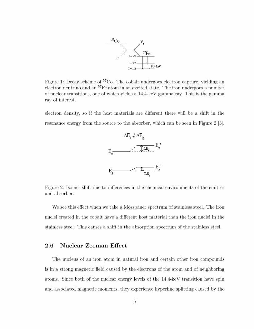
2.4 Use of 57Fe in Mossbauer Spectroscopy
In our Mossbauer spectroscopy experiment we use 57Fe. Our γ-ray source is 57Co,
which decays to 57Fe via electron capture as shown in Figure 1. When the iron decays
from the I=3/2 to the I=1/2 state a 14.4-keV gamma ray is emitted, which is the
photon of interest. For absorbers we use foils of stainless steel and natural iron.
The resolution of the spectrometer is characterized by the ratio ∆EE
. The first
excited state of 57Fe, has a natural line width Γ = 2.4× 10⁻⁹ eV, and the transition
produces a photon of 14.4-keV. Thus, the ideal resolution of our apparatus is 1.7 ×
10−13. The actual resolution of the spectrometer is approximately the measured
linewidth of the stainless steel.
2.5 Isomer Shift
If the chemical environment of the iron nuclei in the source and in the absorber
are different, then the electron densities around the nuclei will be different. The
electromagnetic interaction between the electrons and the nucleus depends on the
4
Figure 1: Decay scheme of 57Co. The cobalt undergoes electron capture, yielding anelectron neutrino and an 57Fe atom in an excited state. The iron undergoes a numberof nuclear transitions, one of which yields a 14.4-keV gamma ray. This is the gammaray of interest.
electron density, so if the host materials are different there will be a shift in the
resonance energy from the source to the absorber, which can be seen in Figure 2 [3].
Figure 2: Isomer shift due to differences in the chemical environments of the emitterand absorber.
We see this effect when we take a Mossbauer spectrum of stainless steel. The iron
nuclei created in the cobalt have a different host material than the iron nuclei in the
stainless steel. This causes a shift in the absorption spectrum of the stainless steel.
2.6 Nuclear Zeeman Effect
The nucleus of an iron atom in natural iron and certain other iron compounds
is in a strong magnetic field caused by the electrons of the atom and of neighboring
atoms. Since both of the nuclear energy levels of the 14.4-keV transition have spin
and associated magnetic moments, they experience hyperfine splitting caused by the
5
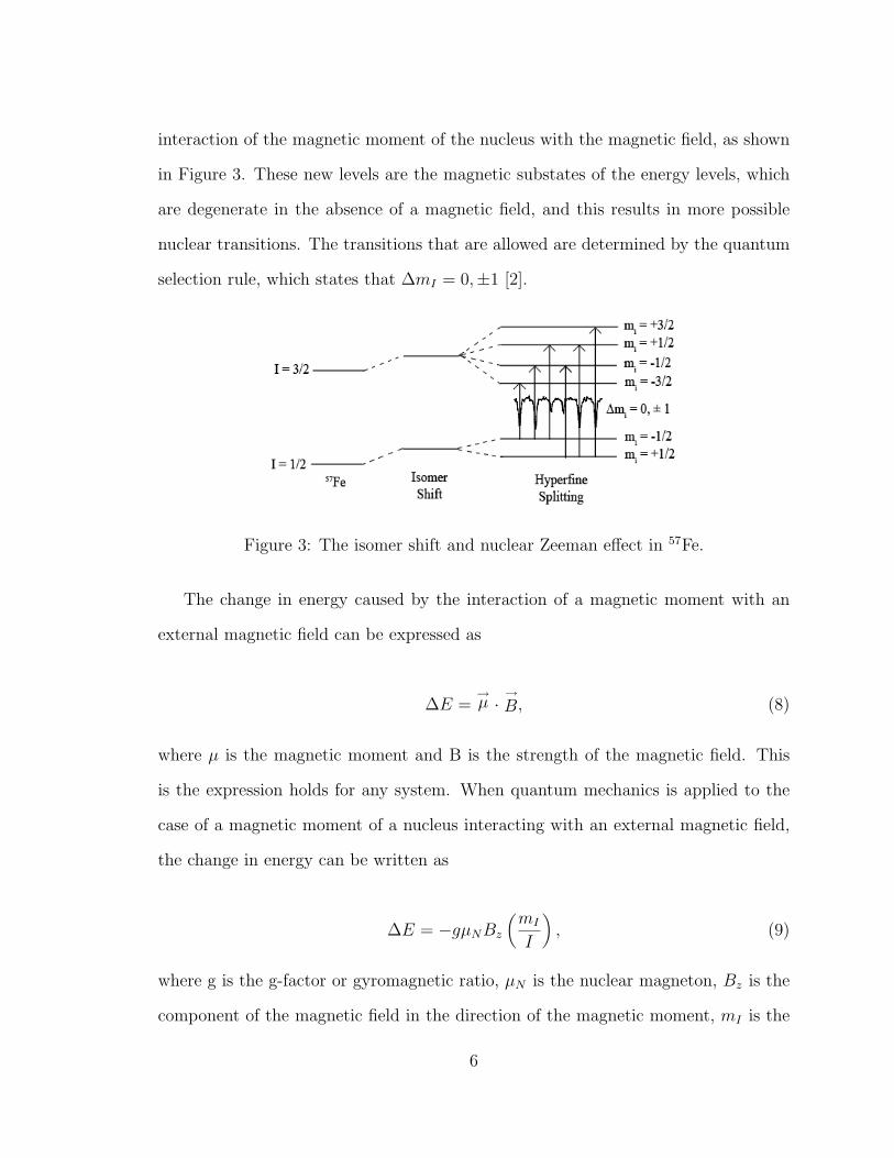
interaction of the magnetic moment of the nucleus with the magnetic field, as shown
in Figure 3. These new levels are the magnetic substates of the energy levels, which
are degenerate in the absence of a magnetic field, and this results in more possible
nuclear transitions. The transitions that are allowed are determined by the quantum
selection rule, which states that ∆mI = 0,±1 [2].
Figure 3: The isomer shift and nuclear Zeeman effect in 57Fe.
The change in energy caused by the interaction of a magnetic moment with an
external magnetic field can be expressed as
∆E =→µ ·
→B, (8)
where µ is the magnetic moment and B is the strength of the magnetic field. This
is the expression holds for any system. When quantum mechanics is applied to the
case of a magnetic moment of a nucleus interacting with an external magnetic field,
the change in energy can be written as
∆E = −gµNBz
(mI
I
), (9)
where g is the g-factor or gyromagnetic ratio, µN is the nuclear magneton, Bz is the
component of the magnetic field in the direction of the magnetic moment, mI is the
6
magnetic substate, and I is the spin of the state. This expression gives us the shift in
energy due to the nuclear Zeeman effect.
The energy of the resulting transitions is
E = (Ee + ∆Ee)− (Eg + ∆Eg) , (10)
where Ee and Eg are the energies of the excited and ground states in the absence
of a magnetic field, and ∆Ee and ∆Eg are the shifts in the energy levels due to the
nuclear Zeeman effect. This expression can be rewritten as
E = Ee − Eg + ∆Ee −∆Eg. (11)
If we set
Ee − Eg = E0, (12)
and
∆Ee −∆Eg = ∆ET , (13)
the expression becomes
E = E0 + ∆ET , (14)
where E0 is the energy of the transition if the levels were not split, and ∆ET is the
energy shift caused by the nuclear Zeeman effect.
7
2.7 Design of Mossbauer Spectrometer
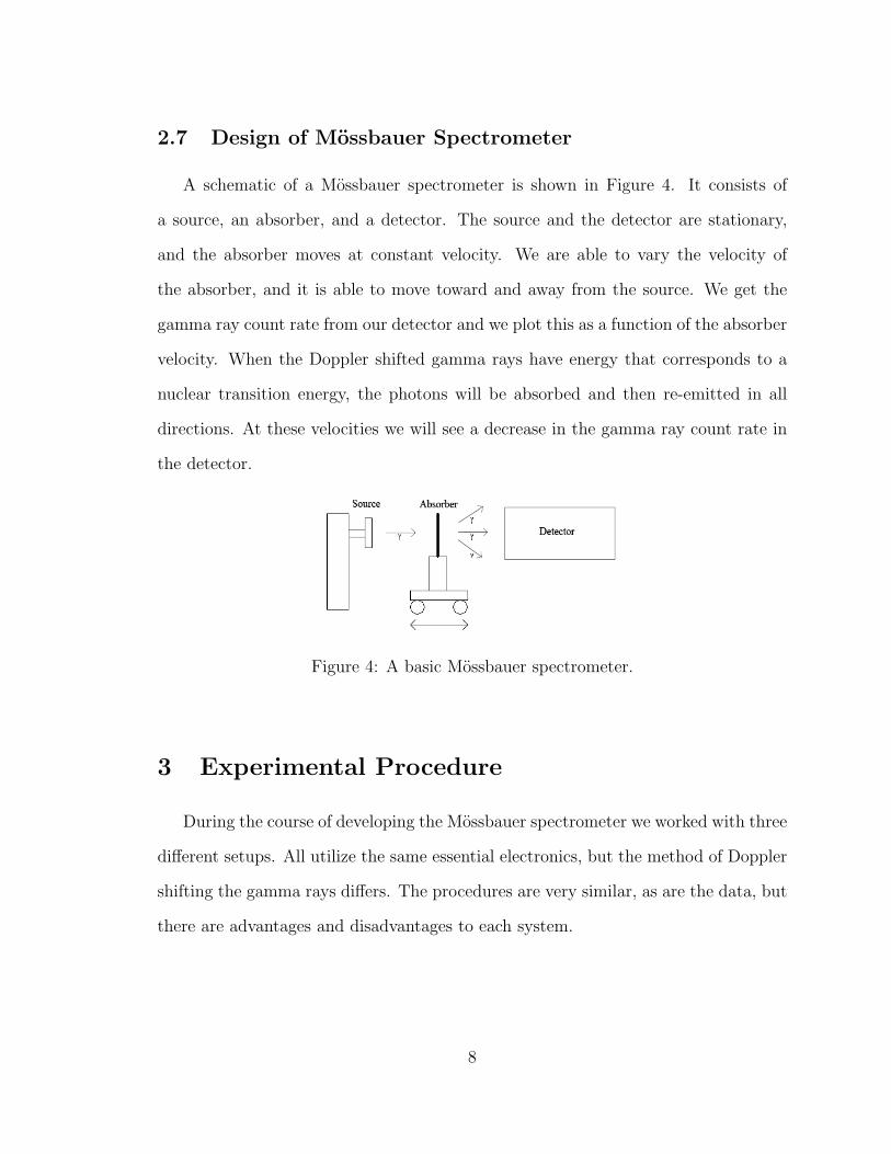
A schematic of a Mossbauer spectrometer is shown in Figure 4. It consists of
a source, an absorber, and a detector. The source and the detector are stationary,
and the absorber moves at constant velocity. We are able to vary the velocity of
the absorber, and it is able to move toward and away from the source. We get the
gamma ray count rate from our detector and we plot this as a function of the absorber
velocity. When the Doppler shifted gamma rays have energy that corresponds to a
nuclear transition energy, the photons will be absorbed and then re-emitted in all
directions. At these velocities we will see a decrease in the gamma ray count rate in
the detector.
Figure 4: A basic Mossbauer spectrometer.
3 Experimental Procedure
During the course of developing the Mossbauer spectrometer we worked with three
different setups. All utilize the same essential electronics, but the method of Doppler
shifting the gamma rays differs. The procedures are very similar, as are the data, but
there are advantages and disadvantages to each system.
8
3.1 Austin Science Associates Setup
A Mossbauer experiment was performed in the Department a number of years
ago, using equipment purchased in the early 1990’s from a company named Austin
Science Associates, which is no longer in operation.
3.1.1 Setup and Procedure
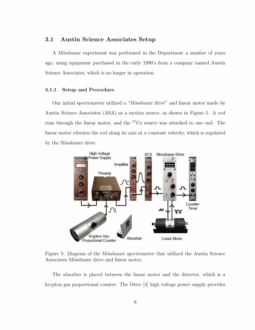
Our initial spectrometer utilized a “Mossbauer drive” and linear motor made by
Austin Science Associates (ASA) as a motion source, as shown in Figure 5. A rod
runs through the linear motor, and the 57Co source was attached to one end. The
linear motor vibrates the rod along its axis at a constant velocity, which is regulated
by the Mossbauer drive.
Figure 5: Diagram of the Mossbauer spectrometer that utilized the Austin ScienceAssociates Mossbauer drive and linear motor.
The absorber is placed between the linear motor and the detector, which is a
krypton gas proportional counter. The Ortec [4] high voltage power supply provides
9
a positive potential on the wire relative to the walls of the detector that sets up an
electric field in the detector. When gamma rays enter the detector they collide with
the krypton atoms, stripping them of some electrons. These electrons are attracted
to the wire, which is at a positive potential relative to the cylindrical housing, and
are accelerated toward it. This causes a current pulse to be emitted from the detector
and is sent to the preamplifier, where it is integrated into a voltage pulse. The height
of this pulse is proportional to the number of electrons collected on the wire, which
is proportional to the energy of the gamma ray.
This signal then goes through an Ortec amplifier, which simply amplifies the signal
to useful voltages, and then the signal is sent to an Ortec single channel analyzer
(SCA). The signal is also sent to a multi-channel analyzer PCI card on a computer.
The gamma ray energy spectrum was acquired with the MCS-32 software on the
computer, and is shown in Figure 6. The signals from the amplifier and the SCA also
go to the PC. The SCA emits a square pulse for every input pulse within a voltage
range that is set on the front panel. The SCA is very important for this experiment
because it assures us that we are only counting the gamma rays of interest. Since the
voltage of the pulse is proportional to the energy of the gamma ray, we are discounting
any gamma rays outside of our range of interest. The signal from the SCA goes to
the computer as well, and the gamma ray energy spectrum gated on the 14.4 keV
gamma ray is shown in Figure 7.
There are also signals sent between the Mossbauer drive and the linear motor.
The Mossbauer drive sends a saw-toothed “drive” signal to the motor. This signal is
essentially a displacement versus time graph and dictates the motion of the motor.
Simultaneously, the motor sends a square “velocity” signal back to drive. This signal
shows velocity versus time, and is used by the Mossabauer drive as a gate to block
gamma ray signals obtained during periods of changing velocity.
10
Figure 6: Gamma ray energy spectrum from the 57Co source.
Figure 7: Gamma ray energy spectrum gated on the 14.4 keV peak.
11
The square signal from the SCA passes through the Mossbauer drive, which gates
the signal based on the velocity of the motor, and into the (Tennelec) counter-timer,
which counts the number of pulses for a predetermined time interval.
In order to obtain a Mossbauer spectrum, we run the motor at a range of velocities,
each for a predetermined period of time, and record the number of gamma rays
counted for each velocity. We were able to run the motor at constant velocities
ranging from -9.99 mm/s to +9.99 mm/s, at intervals of 0.01 mm/s, and we generally
counted for 15 seconds at each velocity.
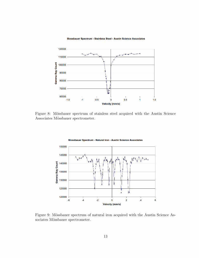
3.1.2 Data
A Mossbauer spectrum for stainless steel is shown in Figure 8. This spectrum
clearly shows one distinct dip in gamma ray count of about 45%. In the absence of
any electromagnetic effects due to the environment of the nucleus, the dip would be
expected at 0.0 mm/s, but is offset a little due to the isomer shift in the steel. There
is one point at -0.1 mm/s which appears to be showing some unexpected behavior,
but after further investigation this point has been determined to be an anomoly.
A Mossbauer spectrum for natural iron is shown in Figure 9. We see six distinct
dips in the gamma ray count ranging from 10-15%. These six dips are due to the
nuclear Zeeman effect, and each one corresponds to a transition in the iron nuclei.
Like the stainless steel, the dips are not symmetric around 0.0 mm/s due to the isomer
shift in the iron.
3.1.3 Advantages and Disadvantages
One of the great advantages to using this setup was that the Mossbauer drive has
a “Constant Acceleration” setting. Instead of recording data at each velocity for a
certain period of time, we could run the motor through a range of velocities during
12
Figure 8: Mossbauer spectrum of stainless steel acquired with the Austin ScienceAssociates Mossbauer spectrometer.
Figure 9: Mossbauer spectrum of natural iron acquired with the Austin Science As-sociates Mossbauer spectrometer.
13
each cycle. The data from the detector and from the Mossbauer drive could be sent
into a multi-channel analyzer card on a computer, which could create a Mossbauer
spectrum automatically. This would make data acquisition a much easier process,
but it might not be as illuminating an experience for the students performing this
experiment in the laboratory course.
One of the disadvantages of this setup is that it is not very transparent for the
students. The motor does not move the rod very far, about 1 cm at most, and
it moves very quickly, so it might be difficult for students to grasp the idea of the
Doppler shift due to the motion of the source. Also, the velocity scale would need
to be calibrated. By looking at Mossbauer spectra acquired by other researchers we
knew that the velocity we set on the Mossbauer drive was not the actual velocity. In
order to make this setup usable we would have had to develop a method for velocity
calibration.
The main disadvantage of this setup, however, is that it stopped working. We
acquired acceptable data, and this would have been useful for the laboratory course,
but unfortunately the Mossbauer drive has ceased operating.
3.2 Speaker-Driven Setup
Many Mossbauer spectrometers have been made using a speaker as the source of
motion for the Doppler shifting, so we decided to try using a speaker and function
generator produced by PASCO Scientific [5], which are primarily used for introductory
physics courses.
3.2.1 Setup and Procedure
After the Mossbauer drive stopped working we wanted to develop something sim-
14
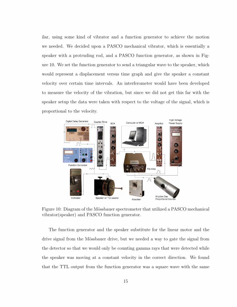
ilar, using some kind of vibrator and a function generator to achieve the motion
we needed. We decided upon a PASCO mechanical vibrator, which is essentially a
speaker with a protruding rod, and a PASCO function generator, as shown in Fig-
ure 10. We set the function generator to send a triangular wave to the speaker, which
would represent a displacement versus time graph and give the speaker a constant
velocity over certain time intervals. An interferometer would have been developed
to measure the velocity of the vibration, but since we did not get this far with the
speaker setup the data were taken with respect to the voltage of the signal, which is
proportional to the velocity.
Figure 10: Diagram of the Mossbauer spectrometer that utilized a PASCO mechanicalvibrator(speaker) and PASCO function generator.
The function generator and the speaker substitute for the linear motor and the
drive signal from the Mossbauer drive, but we needed a way to gate the signal from
the detector so that we would only be counting gamma rays that were detected while
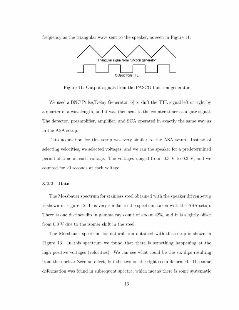
the speaker was moving at a constant velocity in the correct direction. We found
that the TTL output from the function generator was a square wave with the same
15
frequency as the triangular wave sent to the speaker, as seen in Figure 11.
Figure 11: Output signals from the PASCO function generator
We used a BNC Pulse/Delay Generator [6] to shift the TTL signal left or right by
a quarter of a wavelength, and it was then sent to the counter-timer as a gate signal.
The detector, preamplifier, amplifier, and SCA operated in exactly the same way as
in the ASA setup.
Data acquisition for this setup was very similar to the ASA setup. Instead of
selecting velocities, we selected voltages, and we ran the speaker for a predetermined
period of time at each voltage. The voltages ranged from -0.3 V to 0.3 V, and we
counted for 20 seconds at each voltage.
3.2.2 Data
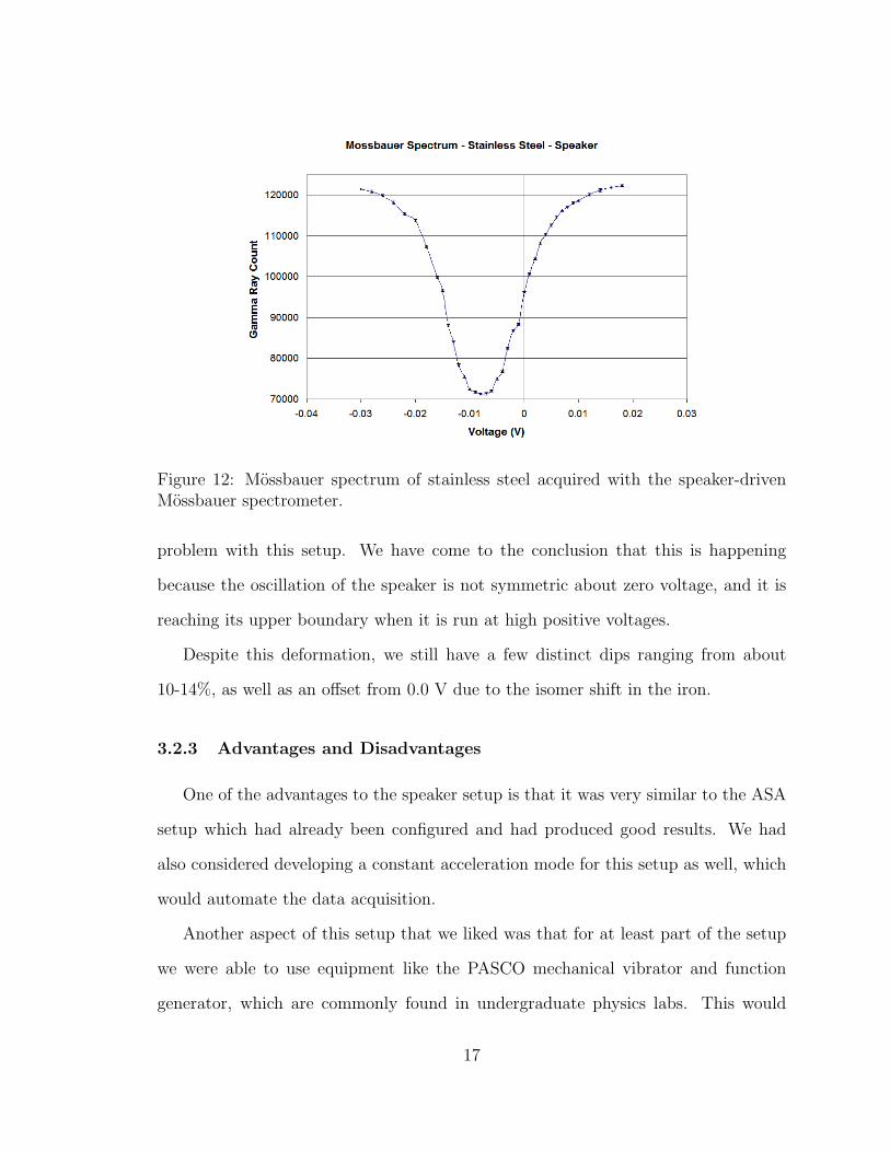
The Mossbauer spectrum for stainless steel obtained with the speaker driven setup
is shown in Figure 12. It is very similar to the spectrum taken with the ASA setup.
There is one distinct dip in gamma ray count of about 42%, and it is slightly offset
from 0.0 V due to the isomer shift in the steel.
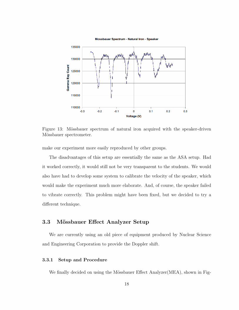
The Mossbauer spectrum for natural iron obtained with this setup is shown in
Figure 13. In this spectrum we found that there is something happening at the
high positive voltages (velocities). We can see what could be the six dips resulting
from the nuclear Zeeman effect, but the two on the right seem deformed. The same
deformation was found in subsequent spectra, which means there is some systematic
16
Figure 12: Mossbauer spectrum of stainless steel acquired with the speaker-drivenMossbauer spectrometer.
problem with this setup. We have come to the conclusion that this is happening
because the oscillation of the speaker is not symmetric about zero voltage, and it is
reaching its upper boundary when it is run at high positive voltages.
Despite this deformation, we still have a few distinct dips ranging from about
10-14%, as well as an offset from 0.0 V due to the isomer shift in the iron.
3.2.3 Advantages and Disadvantages
One of the advantages to the speaker setup is that it was very similar to the ASA
setup which had already been configured and had produced good results. We had
also considered developing a constant acceleration mode for this setup as well, which
would automate the data acquisition.
Another aspect of this setup that we liked was that for at least part of the setup
we were able to use equipment like the PASCO mechanical vibrator and function
generator, which are commonly found in undergraduate physics labs. This would
17
Figure 13: Mossbauer spectrum of natural iron acquired with the speaker-drivenMossbauer spectrometer.
make our experiment more easily reproduced by other groups.
The disadvantages of this setup are essentially the same as the ASA setup. Had
it worked correctly, it would still not be very transparent to the students. We would
also have had to develop some system to calibrate the velocity of the speaker, which
would make the experiment much more elaborate. And, of course, the speaker failed
to vibrate correctly. This problem might have been fixed, but we decided to try a
different technique.
3.3 Mossbauer Effect Analyzer Setup
We are currently using an old piece of equipment produced by Nuclear Science
and Engineering Corporation to provide the Doppler shift.
3.3.1 Setup and Procedure
We finally decided on using the Mossbauer Effect Analyzer(MEA), shown in Fig-
18
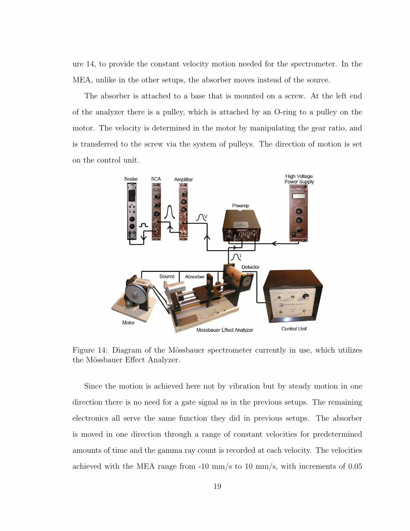
ure 14, to provide the constant velocity motion needed for the spectrometer. In the
MEA, unlike in the other setups, the absorber moves instead of the source.
The absorber is attached to a base that is mounted on a screw. At the left end
of the analyzer there is a pulley, which is attached by an O-ring to a pulley on the
motor. The velocity is determined in the motor by manipulating the gear ratio, and
is transferred to the screw via the system of pulleys. The direction of motion is set
on the control unit.
Figure 14: Diagram of the Mossbauer spectrometer currently in use, which utilizesthe Mossbauer Effect Analyzer.
Since the motion is achieved here not by vibration but by steady motion in one
direction there is no need for a gate signal as in the previous setups. The remaining
electronics all serve the same function they did in previous setups. The absorber
is moved in one direction through a range of constant velocities for predetermined
amounts of time and the gamma ray count is recorded at each velocity. The velocities
achieved with the MEA range from -10 mm/s to 10 mm/s, with increments of 0.05
19
mm/s, and we generally counted for 20 seconds.
In order to calibrate the velocity of the MEA, we set up two photogates a known
distance apart, and measured the time for the absorber to pass between them. We
found that the velocity of on the MEA dial was accurate to within 1%, and we decided
that cailbration was unnecessary.
3.3.2 Data
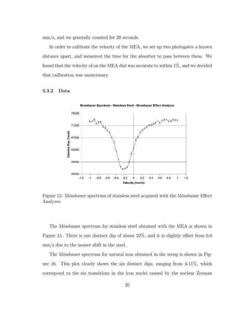
Figure 15: Mossbauer spectrum of stainless steel acquired with the Mossbauer EffectAnalyzer.
The Mossbauer spectrum for stainless steel obtained with the MEA is shown in
Figure 15. There is one distinct dip of about 22%, and it is slightly offset from 0.0
mm/s due to the isomer shift in the steel.
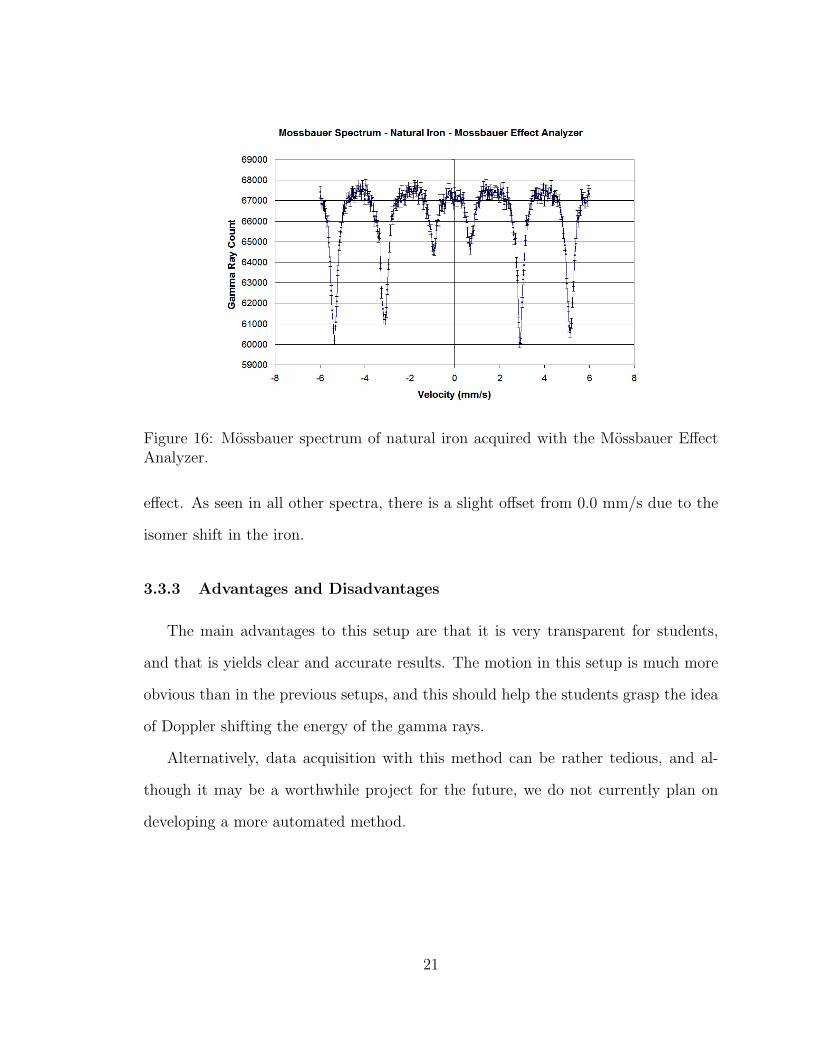
The Mossbauer spectrum for natural iron obtained in the setup is shown in Fig-
ure 16. This plot clearly shows the six distinct dips, ranging from 4-11%, which
correspond to the six transitions in the iron nuclei caused by the nuclear Zeeman
20
Figure 16: Mossbauer spectrum of natural iron acquired with the Mossbauer EffectAnalyzer.
effect. As seen in all other spectra, there is a slight offset from 0.0 mm/s due to the
isomer shift in the iron.
3.3.3 Advantages and Disadvantages
The main advantages to this setup are that it is very transparent for students,
and that is yields clear and accurate results. The motion in this setup is much more
obvious than in the previous setups, and this should help the students grasp the idea
of Doppler shifting the energy of the gamma rays.
Alternatively, data acquisition with this method can be rather tedious, and al-
though it may be a worthwhile project for the future, we do not currently plan on
developing a more automated method.
21
4 Data Analysis
In the lab handout for this experiment, which can be found in Appendix A, we
ask the students to extract several quantities from the Mossbauer spectra they ac-
quire. For the stainless steel absorber, they are instructed to find the linewidth of the
transition and the isomer shift. For the natural iron they are instructed to find the
isomer shift, the g-factor of the excited state given the g-factor of the ground state,
and the strength of the magnetic field at the nucleus.
4.1 Stainless Steel
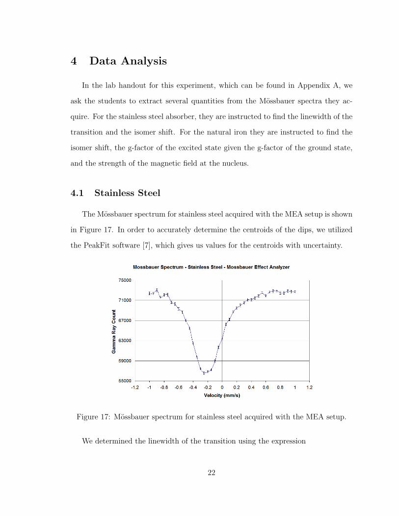
The Mossbauer spectrum for stainless steel acquired with the MEA setup is shown
in Figure 17. In order to accurately determine the centroids of the dips, we utilized
the PeakFit software [7], which gives us values for the centroids with uncertainty.
Figure 17: Mossbauer spectrum for stainless steel acquired with the MEA setup.
We determined the linewidth of the transition using the expression
22
Γ =vfwhm
cEγ, (15)
where vfwhm is the full width at half maximum of the dip in the stainless steel spec-
trum, and Eγ = 14.4 keV. The linewidth was determined to be (1.05 ± .04) × 10−8
eV. The isomer shift in stainless steel was determined using the expression
∆Eisomer =visomer
cEγ, (16)
where visomer is the offset from 0 mm/s in the spectrum. The isomer shift in stainless
steel was determined to be (−1.20± .05)× 10−8eV.
4.2 Natural Iron
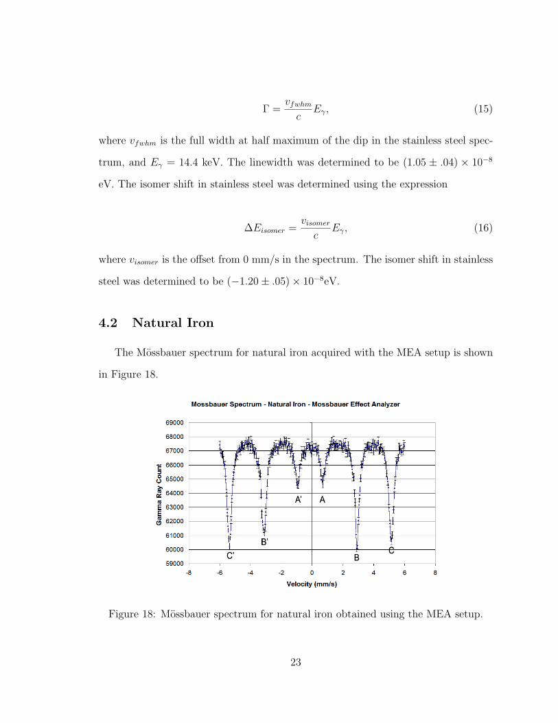
The Mossbauer spectrum for natural iron acquired with the MEA setup is shown
in Figure 18.
Figure 18: Mossbauer spectrum for natural iron obtained using the MEA setup.
23
We will use Equation (16) to determine the isomer shift in natural iron. In order
to determine visomer we averaged the offsets of the three sets of dips. We found the
isomer shift of the natural iron to be (−5± 1)× 10−9eV.
In Equation (14) we defined the energy shift of the transition to be
∆ET = ∆Ee −∆Eg, (17)
where ET is the energy of the transition, Ee is the energy shift of the excited state,
and Eg is the energy shift of the ground state.
If we substitute using Equations (7) and (9) we find
v
cEγ = −geµNBz
(MIe
Ie
)+ ggµNBz
(MIg
Ig
), (18)
where the subscripts ‘e’ and ‘g’ refer to the excited state and ground state respectively.
Solving for the velocity at which each peak occurs we find
vMIg→MIe= −gea
(MIe
Ie
)+ gga
(MIg
Ig
), (19)
where a = cEγ
µNBz.
We will use these expressions for the velocities of the peaks to find an expression
that relates gg and ge
v 12→ 3
2− v 1
2→ 1
2
v 12→− 1
2− v− 1
2→− 1
2
=−gea + gga + 1
3gea− gga
13gea + gga− 1
3gea + gga
, (20)
which yields the expression
ge = −3gg
v 12→ 3
2− v 1
2→ 1
2
v 12→− 1
2− v− 1
2→− 1
2
. (21)
24
Therefore, knowing the ground state g-factor to be 0.09044, we found the excited
state g-factor to be −0.157 ± .003, which is consistent with the accepted value of
-0.1549.
Finally, we want to find the value of the magnetic field strength at the nucleus of
the iron atom. In order to do this we must compensate for the isomer shift in the
iron using the expression
vMIg→MIe− visomer =
c
Eγ
µNBz
[(MIg
Ig
)gg −
(MIe
Ie
)ge
]. (22)
Solving for the magnetic field we get
Bz =Eγ
(vMIg→MIe
− visomer
)cµN
[(MIg
Ig
)gg −
(MIe
Ie
)ge
] . (23)
We found the magnetic field at the nucleus of the iron atom to have a strength of
32.4± .1T.
5 Conclusions
In this experiment we successfully developed a Mossbauer spectrometer, which is
being used in an upper-level undergraduate experimental physics course. Mossbauer
spectroscopy is ideal for undergraduates because it allows students to examine quan-
tum mechanical effects which they learn about in introductory and intermediate
courses.
Mossbauer spectroscopy utilizes the principles of recoilless resonant absorption
and the Doppler effect in order to use gamma rays as a very sensitive probe, which
we can use to measure certain properties of the nucleus.
In the course of developing the spectrometer we tried three different setups before
25
we found one that yielded accurate results and was consistent. In our first Mossbauer
spectrometer we used components produced by Austin Science Associates. This setup
yielded good data, but eventually ceased to operate properly.
In an attempt to recreate he operation of the ASA setup, we substituted a PASCO
Scientific mechanical vibrator and and function generator. While this apparatus
yielded similar results, there was a problem with the motion of the positive velocity.
This caused the positive end of the spectra to be distorted.
We settled on an old device that had been used in the Department a number
of years ago which was produced by Nuclear Science and Engineering Corporation.
This setup yields accurate, consistent results, and operates in a way which is very
transparent to the students.
In this experiment the students are instructed to obtain Mossbauer spectra of
stainless steel and natural iron, and to measure the linewidth and isomer shift of
stainless steel, and the isomer shift, the g-factor of the first excited state given the g-
factor of the ground state, and the value of the magnetic field strength at the nucleus
for the natural iron.
We determined the linewidth of stainless steel to be 1.05 ± .04 × 10−8 eV, and
the isomer shift in stainless steel to be −1.20 ± .05 × 10−8 eV. For natural iron we
found the isomer shift to be −5 ± 1 × 10⁻⁹ eV. We determined the g-factor of the
excited state of natural iron to be −.157± .003, which is consistent with the accepted
value of −.1549 [8]. The magnetic field strength at the nucleus was determined to be
32.4± .1T.
This experiment has already been performed by students in the “Modern Experi-
mental Physics” course. It was apparent that the students understood the operation
of the apparatus as well as the physical properties that they were examining. Their
data was very similar to the data shown above, and their results should agree the
26
values we determined.
There is one aspect of the apparatus that will require future work to sustain this
experiment. The 57Co source has a half-life of 270 days, and had a radioactivity of
10mCi when it was purchased. As the source weakens we will need to count gamma
rays for longer periods of time in order to obtain sufficient data. This time will
increase to a point when the absorber will not be able to run at the higher velocities
because it will hit one end of the device.
A future project on the Mossbauer spectrometer will be to devise a system to
allow the absorber to run continuously back and forth in the apparatus in order to
count for longer periods of time. The control unit of the MEA allows for manual
and automatic control of the absorber direction. Currently we utilize the manual
setting, and select the desired direction. On the automatic setting, the absorber will
automatically change direction when it reaches either end of the apparatus.
One way to allow for longer count times would be to use two counters, and count
for both the positive and negative of a given velocity at the same time, allowing the
absorber to run back and forth for as long as desired. A mechanism would need to
be developed to determine which direction the absorber is moving and to select the
correct counter to send the signal to.
27
Appendix A
Mossbuer Spectroscopy
Physics 300
Winter 2006
1.1 Background Information
Mossbauer spectroscopy is a method for measuring small shifts in nuclear energy
levels with high precision. This method involves the ‘recoilless’ emission and absorp-
tion of gamma rays and utilizes the Doppler effect in order to use these gamma rays
as a sensitive probe.
1.1.1 Resonant Absorption
A quantum system can undergo a transition when it absorbs or emits a photon of
a specific energy. The energy of the photon is dependent upon the difference in the
energy levels of the transition. The energy of the ground state is absolute, but the
energy of the excited state is not a precisely defined quantity. Due to the Uncertainty
Principle, the natural line width is given by
Γ =h
2τ, (2)
where Γ is the natural line width of the excited state and τ is the lifetime of the state.
However, when a photon is emitted by a free system not all the transition energy
goes into the photon. This is because the system recoils due to conservation of
momentum, and takes with it some of the transition energy in the form of kinetic
28
energy. If we call the energy of the transition ET and the recoil energy ER, then the
energy of the emitted photon can be expressed as
Eγ = ET − ER. (3)
We can rewrite this expression in terms of the recoil momentum as
Eγ = ET −p2
R
2m. (4)
Due to conservation of momentum we see that
pR = pγ =Eγ
c, (5)
where pγ is the momentum of the photon.
By combining Equations (4) and (5) we find that the energy of the emitted photon
is
Eγ = ET −E2
γ
2mc2. (6)
Likewise, when the photon is absorbed the absorbing system recoils. Therefore,
the distributions of the emission and absorption energies are separated by twice the
recoil energy. The probability of resonant absorption is proportional to the overlap
of these distributions.
In atomic systems this probability is very high because the recoil energy is small
compared to the natural line widths. In nuclear systems, however, the recoil energy
is much larger than the natural line widths, and therefore the probability of resonant
absorption is very small.
29
1.1.2 Recoilless Emission & Absorption
In 1958, Rudolf Mossbauer showed that for atoms bound in a lattice, a nucleus
doesn’t recoil individually. The recoil momentum, therefore, is taken up by the entire
lattice, which has a very large mass. From equation (6) we see that as m → ∞,
Eγ → ET . Therefore, when the nucleus is embedded in a massive substrate the recoil
energy is negligible. This concept applies to absorption of photons as well.
1.1.3 Doppler Shift
When there is relative motion between the emitter and the absorber there is a
Doppler shift in photon energy. The energy of the photon is given by the Lorentz
transformation
E ′γ =
1√1− β2
(Eγ + vpγ) = Eγ1 + β√1− β2
, (7)
where β = vc, Eγ and pγ are the energy and momentum of the emitted photon, v is
the relative velocity between the emitter and the absorber, and E ′γ is the resulting
Doppler shifted photon energy. For β � 1 we take the first order of the binomial
expansion to get
∆E = E ′γ − Eγ = βEγ =
v
cEγ (8)
as an expression for the change in photon energy due to the motion.
If we are able to vary the relative velocity between the emitter and absorber, we
are able to scan a range of photon energies. In Mossbauer spectroscopy we measure
the absorption rate as a function of velocity, which can be converted to energy shift.
Analysis of the absorption spectrum yields information about the structure of the
30
nucleus.
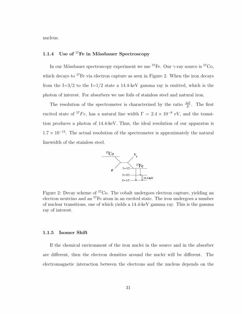
1.1.4 Use of 57Fe in Mossbauer Spectroscopy
In our Mossbauer spectroscopy experiment we use 57Fe. Our γ-ray source is 57Co,
which decays to 57Fe via electron capture as seen in Figure 2. When the iron decays
from the I=3/2 to the I=1/2 state a 14.4-keV gamma ray is emitted, which is the
photon of interest. For absorbers we use foils of stainless steel and natural iron.
The resolution of the spectrometer is characterized by the ratio ∆EE
. The first
excited state of 57Fe, has a natural line width Γ = 2.4 × 10⁻⁹ eV, and the transi-
tion produces a photon of 14.4-keV. Thus, the ideal resolution of our apparatus is
1.7 × 10⁻¹³. The actual resolution of the spectrometer is approximately the natural
linewidth of the stainless steel.
Figure 2: Decay scheme of 57Co. The cobalt undergoes electron capture, yielding anelectron neutrino and an 57Fe atom in an excited state. The iron undergoes a numberof nuclear transitions, one of which yields a 14.4-keV gamma ray. This is the gammaray of interest.
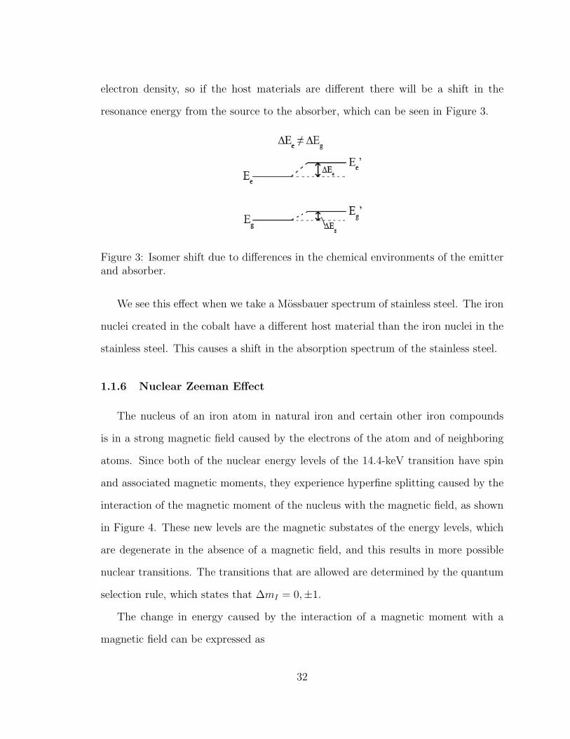
1.1.5 Isomer Shift
If the chemical environment of the iron nuclei in the source and in the absorber
are different, then the electron densities around the nuclei will be different. The
electromagnetic interaction between the electrons and the nucleus depends on the
31
electron density, so if the host materials are different there will be a shift in the
resonance energy from the source to the absorber, which can be seen in Figure 3.
Figure 3: Isomer shift due to differences in the chemical environments of the emitterand absorber.
We see this effect when we take a Mossbauer spectrum of stainless steel. The iron
nuclei created in the cobalt have a different host material than the iron nuclei in the
stainless steel. This causes a shift in the absorption spectrum of the stainless steel.
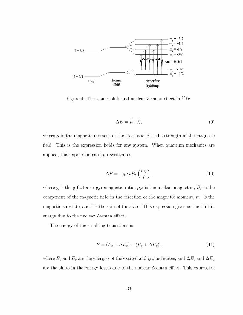
1.1.6 Nuclear Zeeman Effect
The nucleus of an iron atom in natural iron and certain other iron compounds
is in a strong magnetic field caused by the electrons of the atom and of neighboring
atoms. Since both of the nuclear energy levels of the 14.4-keV transition have spin
and associated magnetic moments, they experience hyperfine splitting caused by the
interaction of the magnetic moment of the nucleus with the magnetic field, as shown
in Figure 4. These new levels are the magnetic substates of the energy levels, which
are degenerate in the absence of a magnetic field, and this results in more possible
nuclear transitions. The transitions that are allowed are determined by the quantum
selection rule, which states that ∆mI = 0,±1.
The change in energy caused by the interaction of a magnetic moment with a
magnetic field can be expressed as
32
Figure 4: The isomer shift and nuclear Zeeman effect in 57Fe.
∆E =→µ ·
→B, (9)
where µ is the magnetic moment of the state and B is the strength of the magnetic
field. This is the expression holds for any system. When quantum mechanics are
applied, this expression can be rewritten as
∆E = −gµNBz
(mI
I
), (10)
where g is the g-factor or gyromagnetic ratio, µN is the nuclear magneton, Bz is the
component of the magnetic field in the direction of the magnetic moment, mI is the
magnetic substate, and I is the spin of the state. This expression gives us the shift in
energy due to the nuclear Zeeman effect.
The energy of the resulting transitions is
E = (Ee + ∆Ee)− (Eg + ∆Eg) , (11)
where Ee and Eg are the energies of the excited and ground states, and ∆Ee and ∆Eg
are the shifts in the energy levels due to the nuclear Zeeman effect. This expression
33
can be rewritten as
E = Ee − Eg + ∆Ee −∆Eg. (12)
If we set
Ee − Eg = E0, (13)
and
∆Ee −∆Eg = ∆Etransition, (14)
the expression becomes
E = E0 + ∆Etransition, (15)
where E0 is the energy of the transition if the levels were not split, and ∆Etransition
is the energy shift caused by the nuclear Zeeman effect.
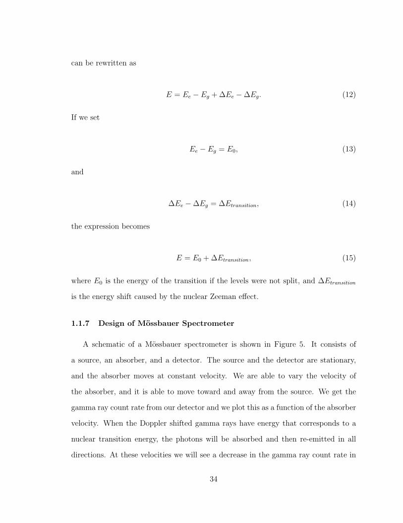
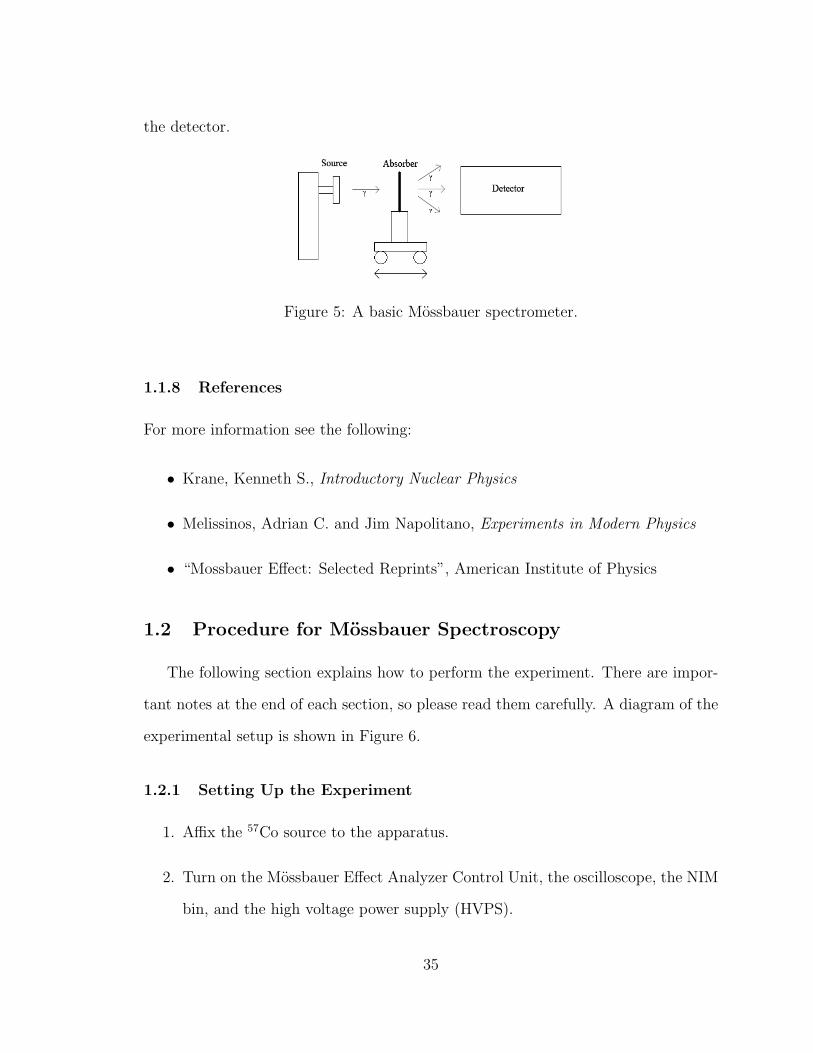
1.1.7 Design of Mossbauer Spectrometer
A schematic of a Mossbauer spectrometer is shown in Figure 5. It consists of
a source, an absorber, and a detector. The source and the detector are stationary,
and the absorber moves at constant velocity. We are able to vary the velocity of
the absorber, and it is able to move toward and away from the source. We get the
gamma ray count rate from our detector and we plot this as a function of the absorber
velocity. When the Doppler shifted gamma rays have energy that corresponds to a
nuclear transition energy, the photons will be absorbed and then re-emitted in all
directions. At these velocities we will see a decrease in the gamma ray count rate in
34
the detector.
Figure 5: A basic Mossbauer spectrometer.
1.1.8 References
For more information see the following:
• Krane, Kenneth S., Introductory Nuclear Physics
• Melissinos, Adrian C. and Jim Napolitano, Experiments in Modern Physics
• “Mossbauer Effect: Selected Reprints”, American Institute of Physics
1.2 Procedure for Mossbauer Spectroscopy
The following section explains how to perform the experiment. There are impor-
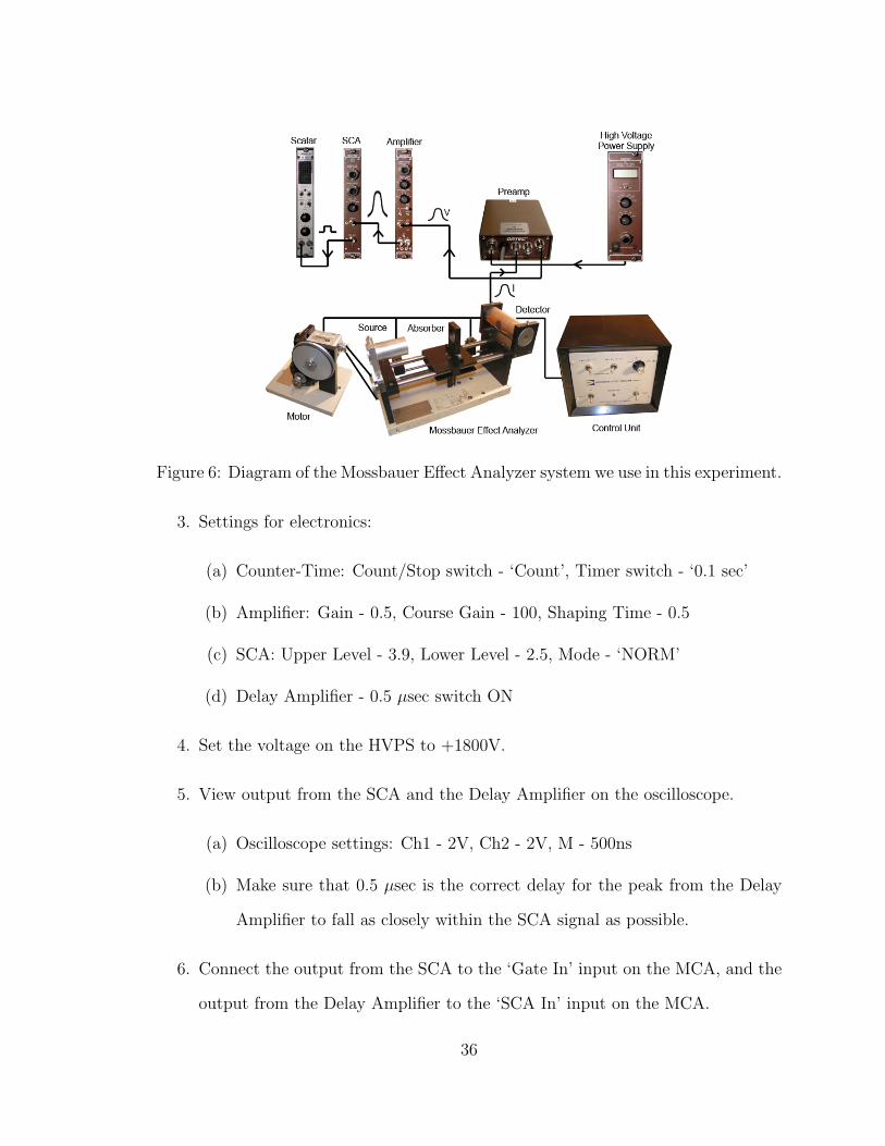
tant notes at the end of each section, so please read them carefully. A diagram of the
experimental setup is shown in Figure 6.
1.2.1 Setting Up the Experiment
1. Affix the 57Co source to the apparatus.
2. Turn on the Mossbauer Effect Analyzer Control Unit, the oscilloscope, the NIM
bin, and the high voltage power supply (HVPS).
35
Figure 6: Diagram of the Mossbauer Effect Analyzer system we use in this experiment.