DEVELOPMENT OF A MUSCULOTENDON MODEL WITHIN THE FRAMEWORK OF MULTIBODY SYSTEMS DYNAMICS Ana Rita Sousa de Oliveira Dissertation to obtain Master Degree in Biomedical Engineering Supervisors: Prof. Miguel Pedro Tavares da Silva Prof. Mamede de Carvalho Examination Committe Chairperson: Prof. M ´ onica Duarte Correia de Oliveira Supervisors: Prof. Miguel Pedro Tavares da Silva Members of the Committee: Prof. Jo˜ ao Orlando Marques Gameiro Folgado Prof. Jo˜ ao Nuno Marques Parracho Guerra da Costa December 2014
Transcript
DEVELOPMENT OF A MUSCULOTENDON MODELWITHIN THE FRAMEWORK OF MULTIBODY SYSTEMS
DYNAMICS
Ana Rita Sousa de Oliveira
Dissertation to obtain Master Degree inBiomedical Engineering
Supervisors: Prof. Miguel Pedro Tavares da SilvaProf. Mamede de Carvalho
Examination Committe
Chairperson: Prof. Monica Duarte Correia de OliveiraSupervisors: Prof. Miguel Pedro Tavares da SilvaMembers of the Committee:
Prof. Joao Orlando Marques Gameiro FolgadoProf. Joao Nuno Marques Parracho Guerra da Costa
December 2014
Agradecimentos
Em primeiro lugar gostaria de agradecer ao meu orientador, Professor Miguel Tavares da Silva,
pelo voto de confianca concedido para realizar este trabalho. A sua orientacao, motivacao e conheci-
mento foram imprescindıveis na realizacao desta tese. Tambem ao Professor Mamede de Carvalho por
fornecer o seu feedback medico e o seu ponto de vista neste trabalho.
Ao Sergio Goncalves que me ajudou, acompanhou ao longo deste perıodo e me transmitiu os seus
conhecimentos para conseguir desenvolver, ultrapassar e interpretar diversos problemas que ocor-
reram.
A todos os meus amigos, em especial a Teresa e Salome por se encontrarem presentes em todos
os momentos ao longo destes anos e pela preocupacao sempre demonstrada.
Ao Joao que durante esta importante etapa da minha vida teve a paciencia de ouvir todos os meus
problemas e possıveis solucoes e pela palavra de encorajamento, sempre presente, perante os meus
nervosismos e medos.
A toda a minha famılia, em especial ao meu tio Henrique por me ter encorajado a seguir o caminho
das ’pernas de pau’. Descobri, com isto, o meu gosto pelo desenvolvimento de tecnologias na area
medica, e principalmente na area de Biomecanica.
Por fim, a minha mae. Agradeco o seu encorajamento, motivacao, presenca e sacrifıcio ao longo de
toda a minha vida. Este trabalho e dedicado a ela.
i
Para a minha mae, Cristina Oliveira.
To my mother, Cristina Oliveira.
Abstract
The main aim of this study is the development of a musculotendon model and its implementation in
a multibody dynamics code with natural coordinates already existent. This model is a Hill-type muscle
model assembled in series with a tendon model and it intends to simulate the dynamic contraction of
the musculotendon unit in order to analyze the interaction between the muscle and the tendon and its
influence in the movement.
To study the mechanics of the human movement, the musculotendon model was integrated in the
code in a forward dynamics perspective that allows for the determination of the system motion for a
given set of muscle activations, and also in an inverse dynamics perspective that allows the calculation
of the muscle activations, and consequently the musculotendon forces, that are needed to execute a
presented movement.
A biomechanical model of the whole body in which the muscle apparatus of the lower limb is con-
stituted by forty-three muscle was developed to analyze the musculotendon model. Experimental data
of gait, running and jumping were acquired in a biomechanics laboratory. The results showed that the
tendon has a significant influence in certain muscle groups along the movements analyzed. The results
are compared with the muscle model and discussed, as well as, some conclusions are taken together
with possible future developments.
Keywords
Multibody dynamics, Inverse and Forward Dynamic, Musculotendon Contraction Dynamics, Muscu-
lotendon Force, Biomechanical Model
v
Resumo
O principal objetivo deste estudo e o desenvolvimento e implementacao de um modelo musculo-
tendao num codigo de dinamica de sistemas multicorpo com coordenadas naturais ja existente. Este
modelo e um modelo muscular do tipo Hill em serie com um tendao que pretende simular a contracao
dinamica da unidade musculo-tendao de forma a analisar a interacao entre o musculo e o tendao e a
sua influencia no movimento.
Para estudar a mecanica do movimento humano, o modelo musculo-tendao foi integrado no codigo
numa perspectiva de dinamica directa, que permite a determinacao do movimento do sistema dado
um conjunto de activacoes musculares, e tambem numa perspectiva dinamica inversa, que permite o
calculo das activacoes musculares, e consequentemente, as forcas musculo-tendao, que sao necessarias
para executar um determinado movimento prescrito.
Foi desenvolvido um modelo biomecanico do corpo inteiro, no qual o aparelho muscular dos mem-
bros inferiores e constituıdo por quarenta e tres musculos. Foram adquiridos dados experimentais de
marcha, corrida e salto em laboratorio de Biomecanica que, em conjunto com o modelo biomecanico
proposto, foram utilizados para calcular a resposta biomecanica do sistema como um todo e do modelo
musculo-tendao desenvolvido em particular para cada um desses movimentos. Os resultados mostram
que o tendao influencia significamente certos grupos de musculos ao longo dos movimentos analisa-
dos. Os resultados sao comparados com o modelo muscular sem tendao e discutidos, assim como, sao
tiradas algumas conclusoes e proposto um conjunto de desenvolvimentos futuros.
Palavras Chave
Dinamica Multicorpo , Dinamica Directa e Inversa, Dinamica de Contracao Musculo-tendao, Forca
The musculotendon system, as the name implies, is composed by skeletal muscle and tendons.
Skeletal muscle is the most abundant tissue in the human body that is able to transform chemical energy
in to mechanical energy (Oatis, 2014) and to provide strength and protection to the skeleton through load
distribution and shock absorbtion.
During a contraction, muscle force that is required to the movement is produced and it is transmitted
to tendons, located at the origin and insertion of the muscle, causing rotation of the bones about the
joints. This force depends on the level of neural excitation provided by the central nervous system
(CNS) and the length and contractile velocity of the muscle.
In this chapter, anatomy of the musculotendon system, and the general principles of the muscle
activation and contraction dynamics are reviewed in order to understand how these two systems interact
to produce coordinated movement. The musculotendon mechanical properties are described in the next
chapter.
2.1 Musculotendon Anatomy
The skeletal muscle is composed by individual muscle fibers (structural unit) connected together
through different levels of collagenous tissue: endomysium that surrounds individual fibers, perimysium
that gathers bundles of fibers into fasciles and epimysium that covers the entire muscle (Figure 2.1)
(Muscle-Tendon Mechanics, 2014). This last collagenous tissue is responsible for the connection be-
tween muscle fibers and both tendon and bone (Pandy &Barr, 2004).
Each muscle fiber is composed by a large number of delicate strands, the myofibrils, that are coated
by the sarcolemma, a delicate plasma membrane (Figure 2.1) (Lorens & Campello).
Figure 2.1: Skeletal Muscle Structure. Retrieved from http://www.humankinetics.com/excerpts/excerpts/muscle-structure-and-function.
Myofibrils are composed by actin (thin) and myosin (thick) filaments contained within units denoted
by sarcomeres (Lorens, T &, Campello) as dipicted in Figure 2.2. The sarcomere is the structural and
10
functional unit of the skeletal muscle that lies between two successive Z discs. Its striated appearance is
due to its composition: I bands that only contain actin filaments, A bands that contain myosin filaments
and actin filaments at the ends where they overlap the myosin and H bands that is a zone in the A bandin
which actin filaments are not overlapping (Figure 2.2a)) (Guyton & Hall, 1956).
When activated by stimuli from the nerve (Van der Liden, 1998), the small projections present in the
side of the myosin filaments (Figure 2.2b)), also called cross-bridges, interact with the actin filaments
inducing contraction (Guyton & Hall, 1956). This contraction is supplied by energy in the form of adeno-
sine triphosphate (ATP) that is created by the mitochondria present in the sarcoplasm, an intracellular
fluid that fills the spaces between the myofibrils during contraction. Close to the sarcoplasm there is
a reticulum, the sarcoplasmic reticulum, that stors the calcium ions (Ca+) needed to the next muscle
contraction (Guyton & Hall, 1956).
Figure 2.2: Myofibril Structure. Retrieved from http://www.freezingblue.com/iphone/flashcards/printPreview.cgi?cardsetID=260042.
Muscle fibers are linked to the bone structure at the origin and insertion points, through aponeuroses
and tendons. The different collagenous tissues and the sarcolemma that is composed, acts as elastic
components allowing the transmission of the force produced by the contracting muscle to the skeleton
via the tendon (Muscle-Tendon Mechanics, 2014).
An aponeurosis is composed of tendinous tissue where the fibers are organized in series and ap-
pended at an angle, the pennation angle (Van der Liden, 1998).
At a certain point an aponeurosis becomes a tendon. This contains collagen, elastin, proteoglycans,
water, and fibroblasts and it is characterized as a fibrous protein due to the abundant presence of Type
I collagen (Pandy & Barr, 2004).
The entire tendon is composed by bundles of fascicles that are made of bundles of fibrils (Figure
2.3). The basic load-bearing structure of tendon is the collagen fibril which is arranged longitudinally, in
11
parallel, to maximize the resistance to tensile forces exerted by muscles. These fibrils are bundles of
microfibrils connected by cross-links, which are biochemical bounds, between the collagen molecules.
The number and state of the cross-links are thought to have a significant effect on the strength of the
connective tissue (Pandy & Barr, 2004).
Figure 2.3: Tendon Structure. Retrieved from (Johnson & Pedowitz, 2006).
2.2 The Musculotendon Physiology
The physiological process responsible to transform an electrical stimuli into muscle contraction, the
excitation-contraction (EC) coupling, will be briefly explained in the following subsections.
2.2.1 Muscle Excitation Mechanism
Muscle fibers have the capability to be excitable and the hability to be activated through stimuli
(Skeletal muscle, 2014). These stimuli, also called action potentials, are electrical impulses that begin
in the frontal cortex of the brain and travel across large pyramidal cells, passing by corticospinal tracts
until, the peripheral muscle is reached (Lorens & Campello).
The action potential, that is associated to a single motor neuron (Figure 2.4), is the outcome of a
voltage depolarization-repolarization phenomenon through the neuron cell membrane. It is initiated in
the soma, the cell’s body, and it goes down along the axon until it reaches the synaptic terminals. This
propagation is explained by an active transport mechanism called Na+- K+ pump (Sodium-potassium
ions pump). With the appropriate stimulation, the voltage in the dendrite of the neuron will become less
negative, which will cause a change in the membrane potential, called depolarization. This will open the
voltage-gated sodium channels and the Na+ will rush in, causing a change of charge. Once inside the
cell, they cause the depolarization of the closed region, allowing the propagation of the action potential.
When the voltage becomes positive the sodium channels close and the voltage-gated potassium channel
opens. This allows the K+ to rush out of the cell, decreasing the voltage until it becomes negative, in a
process called repolarization (Neurobiology, 2014).
The impulse reaches the muscle fiber at a junctional region called the neuromuscular junction (Figure
2.4 ) (Skeletal muscle, 2014). Each motor neuron can innervate multiple muscle fibers, and these
together are called a motor unit (Guyton & Hall, 1956). When the impulse achieves the junction, a
neurotransmitter, called acetylcholine, stored in the synaptic vesicles located in the nerve terminal is
release (Skeletal muscle, 2014) into the motor end plate of the muscle (Pandy & Barr, 2004). Sodium
12
ions will be release into the muscle fibers which will cause the formation of cross-bridges between actin
and myosin filaments in the sarcomeres, allowing the muscle fiber contraction.
Figure 2.4: The motor unit and the neuromuscular junction. Retrieved fromhttp://www.biologycorner.com/anatomy/muscles/notes muscles.html.
2.2.2 Muscle Contraction Mechanism
The mechanism of muscle contraction, is explained by the Sliding-filament theory of contraction. In
Figure 2.5 this theory is demonstrated by showing the relaxed (Figure 2.5a)) and contracted (Figure
2.5b)) state of a sarcomere. In the first one, it can be observed that the ends of the actin filaments
prolong from two successive Z discs, but hardly start to overlap each other. Conversely, in the second
case, the actin filaments were pulled into the myosin filaments, and forces arise due to the interaction of
the cross-bridges between the myosin and the actin filaments.
Figure 2.5: The mechanism of muscle contraction. Retrieved from http://greysanatomycast.info/sliding-filament-theory/.
13
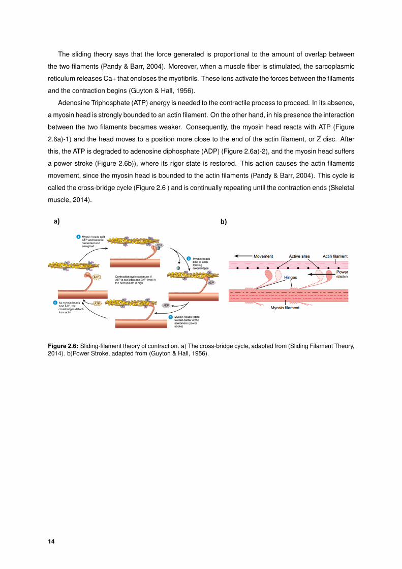
The sliding theory says that the force generated is proportional to the amount of overlap between
the two filaments (Pandy & Barr, 2004). Moreover, when a muscle fiber is stimulated, the sarcoplasmic
reticulum releases Ca+ that encloses the myofibrils. These ions activate the forces between the filaments
and the contraction begins (Guyton & Hall, 1956).
Adenosine Triphosphate (ATP) energy is needed to the contractile process to proceed. In its absence,
a myosin head is strongly bounded to an actin filament. On the other hand, in his presence the interaction
between the two filaments becames weaker. Consequently, the myosin head reacts with ATP (Figure
2.6a)-1) and the head moves to a position more close to the end of the actin filament, or Z disc. After
this, the ATP is degraded to adenosine diphosphate (ADP) (Figure 2.6a)-2), and the myosin head suffers
a power stroke (Figure 2.6b)), where its rigor state is restored. This action causes the actin filaments
movement, since the myosin head is bounded to the actin filaments (Pandy & Barr, 2004). This cycle is
called the cross-bridge cycle (Figure 2.6 ) and is continually repeating until the contraction ends (Skeletal
muscle, 2014).
Figure 2.6: Sliding-filament theory of contraction. a) The cross-bridge cycle, adapted from (Sliding Filament Theory,2014). b)Power Stroke, adapted from (Guyton & Hall, 1956).
The physiological musculotendon behavior, that begins with a neural activation signal and ends with
the muscle contraction (Silva, 2003), is studied in order to understand the dynamics of muscle tissue.
Many mathematical models where developed in order to represent this dynamics with the propose of
accurately analyze the muscle forces exerted during a particular movement.
The dynamics of muscle tissue can be, therefore, divided into activation dynamics and contraction
dynamics (Zajac, 1989), as represented in the next figure (Figure 3.1). The neural excitation u(t), the
stimuli from the CNS, acts through the activation dynamics to create the muscle activation a(t), state of
the internal muscle which is associated with the Ca+ activation of the contractile process. This activation
will give energy to the muscle cross-bridges and muscle force is developed, through musculotendon
contraction dynamics.
Figure 3.1: Muscle Tissue Dynamics.
In the following sections, activation dynamics will be briefly described for completeness reasons,
since it is not implemented in this work. Contraction dynamics will be also explained, and with it the
mechanical properties of the muscle and tendon along with musculotendon mathematical model that
represents muscle contraction dynamics are also presented.
3.1 Activation Dynamics
Activation dynamics corresponds to the transformation of the neural excitation in to muscle activation
(Zajac,1989). Activation dynamics is modelled with a first-order differential equation (Equation 3.1) that
relates the rate change of muscle activation with the neural excitation, i.e. the concentration of ions
inside the muscle with the firing of motor units (Jacobs, 2013).
As mentioned before, a chemical reaction occurs in order for the muscle fiber to begins contracting.
This means that there is a delay between the neural input and the muscle force produced by the muscle,
as illustrated in Figure 3.2 (Robleto, 1997). This equation behaves like a low-pass filter responsible for
introducing this delay (Neptune & Kautz, 2001).
Muscle activation varies continuously between 0, i.e. not excitation, and 1, i.e. full excitation, which
depends on the number of motor units recruited and the firing frequency of these motor units. Like
muscle activation, the excitation signal also vary between 0, i.e. no contraction, and 1, i.e. full contraction
(Jacobs, 2013).
da(t)
dt+ [
1
τact.(β + [1− β]u(t))].a(t) = (
1
τact).u(t) (3.1)
16
Where τact and τdeact = βτact
are the activation and deactivation time constants of a(t), respectively, as
showed in Figure 3.2.
Figure 3.2: Response of a muscle to a neural signal u(t). Image Retrieved from Hirashima (Hirashima et al, 2003).
3.2 Musculotendon Contraction Dynamics
Musculotendon contraction dynamics corresponds to the transformation of muscle activation in to
musculotendon force.
The Hill-type model, presented in Figure 3.3, was used in this work to describe the dynamics of
contraction since it considers the mechanical properties of the muscle and tendon, i.e, force-length-
velocity properties of the muscle and the elastic properties of the tendon (Zajac, 1989).
Figure 3.3: Mechanical Musculotendon Model that describes the musculotendon contraction dynamics.
In this mechanical model, it was assumed that all muscle fibers are parallel and does the same
pennation angle α with the tendon. This angle varies over time in order to guarantee that muscle
thickness lW remains constant.
17
The musculotendon length, that is represented by lMT , results from the sum of tendon length lT and
muscle fibers length lM taking into to account the pennation angle, as represented in Equation 3.2.
lMT = lT + lM cos(α) (3.2)
The tendons and the connective tissues in and around the muscle belly are viscoelastic structures
that allow for the determination of the mechanical properties of the muscle during contraction and pas-
sive extension. The tendon is defined as a spring-like elastic component with a constant stiffness Kt that
depends on its elastic properties, placed in series with the contractile component (Lorenz & Campello).
But its turn, the muscle is represented by a contractile element (CE) in parallel with passive one (PE).
The CE is used to simulate the active muscular action produced by the sarcomeres and the viscous force
developed by the intracellular and intercellular fluid in the muscle. This element produces a force that
depends on the force-length-velocity relation of the muscle and on the activation level. Regarding the
PE, which is used to simulate the elastic properties of the muscle (i.e., the different levels of collagenous
tissue) (Silva,2003), generates a force that depends only on the muscle length. The sum of the forces
generated in these two components, represents the resultant muscle force (Equation 3.3).
FM = FMCE + FMPE =fl(lM )fv(vM )
FM0aM + FMPE(lM ) (3.3)
Where FM is the resultant muscle force, FMCE and FMPE are the contractile and passive muscle force,
respectively, fl(lM ) and fv(vM ) are the force-length and force-velocity relation of the muscle, and aM is
the muscle activation.
As stated in Section 2.1, the force produced by the muscle is transmitted to the skeleton by the
tendon, so the force that is exerted by the tendon, or musculotendon unit, is the one responsible for the
movement. If the pennation angle is zero, i.e. the tendon and the muscle fiber are aligned, therefore,
tendon’s force exerted in the skeleton is equal to the muscle force developed. Otherwise, the tendon
force depends on the pennation angle between both, as expressed in Equation 3.4
FMT = FT = FM cos(α) (3.4)
3.2.1 Force-Length Property
The steady-state (static) properties of muscle tissue are characterized by its isometric fl curve, that
is achieved when the activation and fiber length are held constant (Zajac, 1989). A steady force is de-
veloped when a muscle is maintained isometric and fully activated (Pandy & Barr, 2004). The difference
between the force developed when muscle is activated and when muscle is passive is called active
muscle force. This force is generated when the muscle fiber length is between 0.5lM0 and 1.5lM0 , where
lM0 is the muscle fiber resting length or optimal muscle fiber length. It is the length at which the active
muscle peaks, i.e. FM = FM0 , where FM0 is the maximum isometric force developed by the muscle
(peak isometric active force).
18
The passive muscle begins to developed force at length lM0 as showed in Figure 3.4a). Recent data
suggest that this passive force is due to the intrafiber elasticity (Zajac, 1989).
Figure 3.4: Active and Passive Muscle Force-length relationship. a)Active Muscle Force-length relationship whenthe muscle is fully-activated. b)Active Muscle Force-length relationship when activation level is halved.
When the muscle is not fully activated, the force-length relationship can be regarded as a scaled-
down version of the one that is fully activated, as illustrated in Figure 3.4b).
The shape of the active force-length curve is explained by the muscle contraction mechanism, de-
scribed in the previous chapter. The active muscle force varies with the amount of the thick and the thin
filaments overlap (Pandy & Barr, 2004). Figure 3.5 exhibits the muscle force versus striation spacing
curve, where it is possible to conclude that the active muscle force varies with the muscle fiber length.
Figure 3.5: Active muscle force versus striation space. Image Retrieved from (Pandy & Barr, 2004).
3.2.2 Force-Velocity Property
The fully activated muscle tissue when it is subjected to a constant tension, it shorten and then stops.
Subjecting the muscle to different tension, a set of trajectories are obtained allowing the construction of a
force-velocity (fv) relationship for any length lM , where 0.5lM0 < lM < 1.5lM0 (Figure 3.6a)). A maximum
shortening velocity v0 can be defined at optimal fiber length lM0 , so that muscle cannot hold any tension,
19
even if fully activated (Zajac, 1989).
When the muscle is not fully activated, the force-velocity relationship can also be regarded to be a
scaled-down version of the one that is fully activated, as it is depicted in Figure 3.6b).
Figure 3.6: .
Force-velocity relationship curve for muscle. a) Force-Velocity relationship curve when the muscle is
fully-activated. b)Force-Velocity relationship curve when activation level is halved.
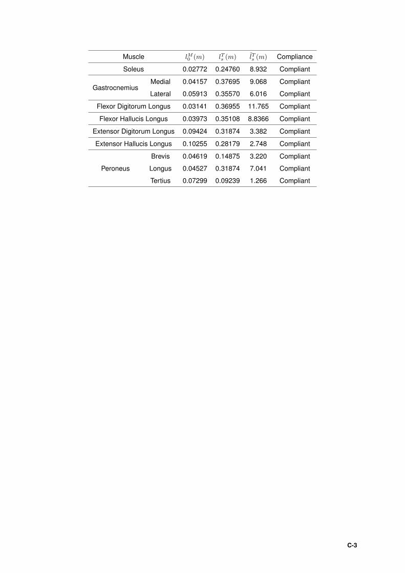
3.2.3 Elastic Properties of Tendon
When a tensile force is applied to a tendon at its resting length (tendon slack length), the tissue
stretches (Pandy & Barr, 2004). The amount of stretched tendon is called tendon strain and is defined
by Equation 3.5.
εT =∆lT
lTs=lT − lTslTs
(3.5)
Where lTs is the length at which tendon starts to produce force and is called tendon slack length.
The normalization of tendon slack length lTs by optimal fiber length lM0 is denoted by lTs and defines
the compliance of the tendon, once the tendon elasticity is proportional to lTs (Zajac, 1989). Thus the
tendon is considered compliant when lTs is higher than 1, and stiff if otherwise.
The tendon’s stiff (lTs ≤ 1) will be treated as inextensible which implies that its length does not change
over time, i.e., it is always equal to the slack length, and as so the tendon velocity is zero.
On the other hand, a compliant tendon will be described by a force-strain curve (Figure 3.7). This
curve presents three characteristic regions: the toe region, the linear region and the failure region.
The toe region is the initial part of the force-strain curve and describes the nonlinear behaviour of the
material. It is caused mainly by the straightening of the collagen fiber (Spyron & Aravas, 2011) that will
cause the modulus of elasticity (slope of the curve) to increase with strain (Zajac, 1989). The linear
region describes the elastic behavior of the tissue, and the constant slope of the curve defines the
modulus of elasticity of the tendon. The failure region describes plastic changes experience by the
20
tissue, where, initially, a few fibrils start to rupture,and lastly the whole tissue fails (Pandy & Barr, 2004).
Over the past thirty years, the development of dependable mathematical models of the human body
for the biomechanics community has been of greater interest to simulate and analyze the mechanical
behaviour of the human body in their day to day activities. This sort of simulation is very important in a
set of applications like, athletic sports, to improve the performance and to optimize the design equipment;
ergonomic studies, to evaluate conditions for comfort and efficiency of the interaction between the human
body and the environment; and orthopedics, to create and analyze prosthesis.
This mathematical models of the human body, also called biomechanical models, describes the hu-
man body in terms of its anthropometry, physiology and topology, that vary depending on the objectives
of the analysis.
In this work, a whole body response biomechanical model are defined using the multibody formula-
tion described in Chapter 4. In the following chapters, the biomechanical model used will be described
in detail taking into to account its anthropometric data, that include the body size segments, the mass,
inertia and center-of-mass location of the principal anatomical segments, and muscle apparatus. Also,
the way that will be implemented will be outlined.
5.1 Model Description
The main propose of this work is to develop a model that allow the study of the main kinematic and
dynamic patterns during different types of human activities like walking, running and jumping. Due to
its complex kinematic structure, it can be used to simulate human movements in forward and inverse
dynamics analysis.
The defined model divides the whole body in eight segments: the HAT, composed by head, arms and
torso, the pelvis, composed by L4-L5 to greater trochanter (Winter, 2000), thigh, leg and foot (Figure 5.1
a) and c)).
The HAT, adapted by the model implemented by Anderson and Pandy (Anderson & Pandy,2007),
was considerer as a single rigid body as seen in Figure 5.1 c).
46
Figure 5.1: Biomecanical Model. a)Human Skeletal Image Retrieved from OpenSim (Delp et al 2007). b)FootSkeletal. Image Retrieved from OpenSim (Delp et al 2007). c)Biomecanical Model Division
The foot was described using the model implemented by Malaquias (Malaquias, 2013). It is divided in
three segments: the rear-foot, that includes the calcaneus; the mid/fore-foot, that includes the Navicular,
cuboid, the three cuneiform bones and metatarsus; and the toes, that are composed by the phalanges
(Figure 5.1 b) and c) ).
The different segments are connected through a set of 13 joints:
1. Pelvis Joint
2. Hip Joint
3. Knee Joint
4. Talocrural joint
5. Talocalcaneal or subtalar joint
6. Midtarsal or Chopart’s joint
7. Metatarsophalangeal joint
The insertion of the mid/fore foot in the model increase the reliability, allowing the study of the move-
ments that occurs between the midtarsal and tarsometatarsal joint. Also, to decrease the integration
time of the model, the talus was consider as a massless link, which means that the axis of the Talocrural
and the talocalcaneal joint do not intersect and have a constant distance between them (Malaquias,
2013).
This model has therefore 27 degrees-of-freedom (DOF). Once they are associated with the type of
motion that each joint is able to realize. They result from:
• 2 DOF - Flexion/Extension and lateral extension at the Pelvis Joint;
• 2× 2 DOF - Flexion/Extension and Abduction/Adduction at the hip joint;
• 2× 1 DOF - Internal thigh rotation;
• 2× 1 DOF - Flexion/Extension of the Knee Joint;
47
• 2× 1 DOF - Internal leg rotation;
• 2× 1 DOF - Inversion/Eversion at the talocalcaneal joint;
• 2× 1 DOF - Flexion/Extension at the talocrural joint;
• 2× 1 DOF - Internal mid-foot and fore-foot rotation;
• 2× 2 DOF - Flexion/Extension and Abduction/Adduction at the Midtarsal joint;
• 2× 1 DOF - Flexion (plantar/dorsiflexion) at the Metatarsophalangeal joint;
• 3 DOF - Rotation and Translation over the three axes of the model.
Figure 5.2 and Figure 5.3 shows the DOF associated with the rigid body described in this model.
Figure 5.2: DOF of the body segments (Silva, 2003).
48
Figure 5.3: DOF of the foot (Malaquias, 2013).
5.2 Implementation Model
Since this model has to be used in forward but mainly in inverse, the model that was implemented
by Silva (Silva, 2003) was adopted. In this model the kinematic structure of rigid bodies and nominal
joints are define in a different way in order to produce a specified combination of flexion/extension,
adduction/abduction and internal/external rotation. For that a set of nominal axes are associated to each
joint. Taking into account the kinematics of a revolute joint, the nominal joint axis is always associated
to the unit vector used to define it. On the other hand, a spherical joint, can not be defined in the same
way since there are no unit vectors to which associate the nominal joint axes (Silva, 2003). A spherical
joint is then substituted by an equivalent joint called composite joint, that is made of a revolute and a
universal joint.
With this new definition, a revolute joint will be use to study the movements that will occur in the knee
joint, talocalcaneal or subtalar joint, talocrural joint and in the Metatarsophalangeal joint. A universal
joint will be used to study sagittal and horizontal movements of the Pelvis Joint, midtarsal or chopart’s
joint and of the ankle joint. Finally, a composite joint will be used in the hip joint.
For define this type of joint a new rigid body must be added, like is seen in Figure 5.4, which implies
an increase in the number of rigid bodies, generalized coordinates and kinematic constraints. This
coincident rigid bodies that are added allow the study of internal rotation. This Biomechanical Model is
therefore define by 20 rigid bodies, 26 points and 29 unit vectors (Figure 5.4).
49
Figure 5.4: Biomechanical Model.
5.3 Anthropometric Data
The anthropometric data is essential for the construction of the biomechanical model. The following
subsections will described the length, mass, center-of-mass location and moments of inertia of each
rigid body that characterize the model.
5.3.1 Segment Dimensions and Center-of-mass location
As illustrated in Figure 5.1b), the anatomical segments are represented by lines, so their dimension
will be the straight-line distance between joint center of rotation. The Table 5.1 shows the segments
length in percentage of total body height (LT ) and of the total foot length (LfP ) relatively to the foot to
obtain the dimensions of the body segments of a particular subject. Also, shows the percentage of the
distance of the center-of-mass (CM) with respect to the proximal joint. An illustration is present in Figure
5.5 to easily understand the table .
50
Table 5.1: Body Segments length in percentage of the body height (LT ) and foot length (LfP ) that defines theBiomechanical model and the respective CM (Winter, 2000; Malaquias, 2013)
Figure 5.5: a)Body Segments length in percentage of the body height (LT ) and foot length (LfP ). b) and c) CMlocation in percentage of the body segment length.
5.3.2 Segment Mass and Inertial Moments
As well as the previous subsection, the mass and principal moments of inertia can be determine
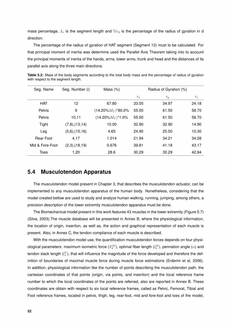
according to scaled values already tabulated (Winter, 2000; Malaquias, 2013). Table 5.2 exhibits the
percentage of mass of a segment relatively to the total body weight (MT ) and the percentage of radius
of gyration in the x, y and z direction with respect to the body segment length in order to determine the
principal moments of inertia. When the body segments numbers presents are between bracket mean
that the percentage present are relative to the sum of both segments.
The principal moments of inertia can be calculated according to the equation (Equation 5.1) present
in De Leva (De Leva, 1996).
Id = M.%mi(Li.%rd)2 (5.1)
Where Id is the moment of inertia in d direction, M is the total mass of the subject, %mi is the segment
51
mass percentage, Li is the segment length and %rd is the percentage of the radius of gyration in d
direction.
The percentage of the radius of gyration of HAT segment (Segment 12) must to be calculated. For
that principal moment of inertia was determine used the Parallel Axis Theorem taking into to account
the principal moments of inertia of the hands, arms, lower arms, trunk and head and the distances of its
parallel axis along the three main directions.
Table 5.2: Mass of the body segments according to the total body mass and the percentage of radius of gyrationwith respect to the segment length.
Seg. Name Seg. Number (i) Mass (%) Radius of Gyration (%)
This chapter is divided in two sections. A first one that describes the acquisition protocol used to
obtain the data needed to do the kinematic evaluation, i.e., angles between segments, and a kinetic
evaluation, i.e., ground reaction forces that are acquired to study the internal reaction forces and the
moments in a inverse dynamic perspective. The second one outlines the data treatment protocol used
to treat the data acquired to have all ready to include the muscle and analyze the results with the use of
the musculotendon model.
This procedure was performed with 1 male subject who were randomly chosen from a group of
healthy college student. He aged 23 years old and don’t have previous history of trauma at the lower
limb. In Table 6.1, information about the subject is described.
Table 6.1: Description of the Markers set protocol. (s) Markers means that they were only used in static acquisition
Subject Age [years] Height [m] Weight [kg]
Male 23 1.7515 75.9
The procedure to perform was explain to the subject. They were subjected to an analysis of walking,
running and jumping.
6.1 Acquisition Protocol
Initially, a kinematic data acquisition was performed using a markers protocol at the Lisbon Biome-
chanics Laboratory (LBL) in Instituto Superior Tecnico. The data were acquired through a system of
fourteen infrared reflective cameras that exist in the laboratory - Qualisys ProReflex and two video cam-
eras. The acquisition software used to control this camera system was the Qualisys Track Manager
(QTM) version 2.9 software. To obtain the data from the external forces result from the movement in
analyze, three force platforms - AMTI-OR6-7 - were used. The cameras and the force plates use a
sampling frequency of 100Hz and 1000Hz, respectively.
In this protocol, to tracking the movement, 54 markers were placed at specific anatomical points of
interest for this study, where 4 of them were only used for static acquisition, as seen in Figure 6.1 and
Table 6.2. The markers used is this analysis were passive markers with flat bases and 19 mm and 11
mm of diameter (the last ones were only used to static acquisitions). This markers reflected IR light that
is emitted and detected by the cameras, because they are made of polystyrene hemispheres covered
by a special retro-reflective tape.
56
Figure 6.1: Markers Set protocol. a)Frontal view. b)Back view. c)Foot top view
Markers placement was based on the protocol developed by Malaquias (Malaquias, 2013) and
Goncalves (Goncalves, 2010) work. Some changes in those marker set protocols was performed in
order to define the biomechanical model described in Section 5.2. Once the arms, torso and head
were defined as a single rigid body, some markers used to defined those, mainly in arms and head, in
Goncalves protocol (Goncalves, 2010) are not used.
Table 6.2: Description of the Markers set protocol. (s) Markers means that they were only used in static acquisition
Marker #Anatomical Landmark
Right Left
1 53 Medial aspect of the hallux
2 52 Top head of the phalange II
3 51 Medial aspect of the head of metatarsal I
4 50 Lateral aspect of the head of metatarsal V
5 49 Medial apex of the tuberosity of the navicular
6 48 Lateral apex of the tuberosity of the cuboid
7 47 Apex of the medial malleolus
8 46 Apex of the lateral malleolus
9 45 Posterior aspect of the calcaneus
10s 44s Super-medial aspect of the talus
11s 43s Posterior lateral ”corner” of the heel
12-15 39-42 Leg Cluster
57
Continuation of Table 6.2
16 38 Most prominent point of lateral femoral epicondyle
17 37 Most prominent point of medial femoral epicondyle
18-21 33-36 Thigh Cluster
22 32 Center of acetabulum
23 31 Asis
24 30 Psis
25 29 Belly
26 28 Clavicle-acromion
27 Spinous process of C7
54 Belly Back
6.2 Data Treatment Protocol
The data acquired in the laboratory must be processed in order to perform a kinematic and kinetic
analysis. Through QTM software a .tsv file, i.e. a table-separated value file, is obtained with the markers
trajectory that were acquired. The markers were identify depending on their location to define an Auto-
matic Identification of Markers (AIM) to guarantee an efficient assignment of the trajectories. Each file
contain the trajectory corresponding to a cycle of analysis, initial contact of the foot with the force plate
for the gait and run and preparation phase, corresponding to the moment when the center of mass of
the subject descends to the ground for the jump.
A routine in Matlab was developed to treat the data. Fist, a third order low pass digital Butterworth
filter with a cut frequency of 6Hz for the gait and run, and 10 Hz for the jump was applied. It is important
for this step have at least 10 frames before and after the cycle under analysis to be discarded and to
perform a correct filtering.
After filtering, a set of steps had to be followed to create a modulation (.mdl), simulation (.sml), data
(.dat) and forces (.frc) files, needed to perform a inverse dynamic analysis. The following chapters will
explain the ones adopt to determined the variables needed to each file.
6.2.1 Modulation File
The modulation file describes the masses, inertias (Table 5.2), local coordinates of the points related
to the mass center (Table 5.1) and of the unit vectors that defines each rigid body of the biomechanical
model. Also contains the parameters that define the drivers that guide each DOF, the inner product and
superpositions constraints and the muscle apparatus (Annex B).
Through markers position, the joint centers and unit vectors coordinates were determined. Consid-
ering Figure 6.1, a formula use to determine each point and unit vectors will be describe in Table 6.3
and Table 6.4, respectively.
58
Table 6.3: Joint centers that describe the Biomechanical model. Mi represent the coordinates of the respectivemarker. The formulas present only takes into account the markers of the right, but the procedure to left one is thesame.
Pi Formula Pi Formula
P1 M∗2 P8M7+M8
2
P2 ≡ P3M3+M4
2 P9 ≡ P10M16+M17
2
P4 ≡ P5M5+M6
2 P11 ≡ P12 M22,M32,M23,M31,M54
P6 M9 P14M25+M29
2
P7M10s+M11s
2 P15M25+M28
2
Note: M∗2 is constitute by the x,y coordinates of M2 and by the z coordinate of M1
The hip joint center (P11 ≡ P12 and P13 ≡ P17) was determined through the algorithm developed by
Davis et al (Davis et al, 1991). This algorithm consist in determine the distance of the hip joint center
relative to the center of the embedded coordinate system of the pelvis obtained thought at least three
non-collinear markers attached to it, the markers positioned in ASIS, PSIS and belly back.
Table 6.4: Vectors that describe the model. The formulas present only takes into account the markers of the right,but the procedure to left one is equal. All the vector were normalized
Description Segment iKinematic Vectors Unit Vectors
Formula(Global RF) (Local RF)
HAT12
vShoulder M26 −M28
zHAT P15 − P14
xHAT v27 (zHAT × vShoulder)
yHAT v14 (zHAT × xHAT )
Pelvis 10,11
vPelvis P17 − P11
xPelvis1 v11, v12, v15, v16 xThigh1
yPelvis1 (xPelvis1 × vPelvis)
zPelvis1 vPelvis
Pelvis 9
vzPelvis P14 − P17+P11
2
xPelvis v13 (vPelvis × vzPelvis)
yPelvis v29 vPelvis
zPelvis v28 (xPelvis × yPelvis)
Thigh 8,14
zThigh1 P9 − P11
xThigh1 (vPelvis × zThigh1)
yThigh1 (zThigh1 × xThigh1)
Thigh7,13
vKnee v10, v8, v17, v19 M16 −M17
zThigh2 P9 − P11
xThigh2 (zThigh2 × vKnee)
yThigh2 (zThigh2 × xThigh2)
59
Continuation of the Table 6.4
Leg 6,16
vTalocrural v6, v20 M8 −M7
zLeg1 P9 − P8
xLeg1 (xLeg1 × vKnee)
yLeg1 (zLeg1 × xLeg1)
Leg 5,15
vMidtarsal M6 −M5
zLeg2 P9 − P8
xLeg2 v7, v18 (zLeg2 × vMidtarsal)
yLeg2 (zLeg2 × xLeg2)
Rear-foot 4,17
vTalocalcaneal v5, v22, v22 M10s −M11s
xRFM5+M6
2 −M9
zRF (vMidtarsal × xRF )
yRF v4, v21 (zRF × xRF )
Mid- & Fore-foot 2,19
vMetatarsophalangeal v1, v2, v25, v23 M4 −M3
xMFFF1 P3 − P4
zMFFF1 (vMetatarsophalangeal × xMFFF1)
yMFFF1 (zMFFF1 × xMFFF1)
Mid- & Fore-foot 3,18
xMFFF2 P3 − P4
zMFFF2 v3, v24 (vMidtarsal × xMFFF2)
yMFFF2 (zMFFF2 × xMFFF2)
Toes1,20
xToes M∗2 − M3+M4
2
zToes v9, v26 (vMetatarsophalangeal × xToes)
yToes (zToes × xToes)
The transformation of the vectors from global reference frame to local reference frame was performed
through Equation 6.1.
vLFi = A−1vGFi (6.1)
Where vLFi and vGFi are the vectors in the local and global reference frame, respectively, and A−1 is
the transformation matrix that is composed by the vectors that define the local reference of a rigid body
(Equation 6.2), determined in Table 6.4.
A = [xTRB yTRB zTRB ] (6.2)
RB is the respective rigid body.
6.2.2 Simulation File
The simulation file presents the initial state of the system, i.e., positions, velocities, Tait-Bryan angles
and angular velocity of each rigid body, related to the center of mass in the global reference frame. Also,
60
addressed the time parameters, the gravity field vector and the optimization procedure definition.
The positions coordinates are obtained through the relation present in Equation 6.3.
PRBCM = Pi +Asi (6.3)
PRBCM is the coordinates of center of mass in the global reference frame of rigid body RB, Pi is the
coordinates in the global reference frame of a joint center i that defines the rigid body, obtained in Table
6.3, A is the transformation matrix and si is the position of the joint center i related to the center of mass
in the local reference frame (Table 5.1).
The Tait-Bryan angles with a sequence of rotation Z-Y-X will described the orientation of the seg-
ments. The sequence of rotation defines the order of rotation about the axis. First the segment will
suffer a positive rotation φ about the z-axis, second a positive rotation θ about the y’-axis and finally, a
positive rotation ψ about the x”-axis, resulting in the final system (Laananen el al, 1983). Through the
matrix (Equation 6.4) that results of these sequence and the transformation matrix obtained above the
The data file contains the angles over time that drives the model. Each file can contain one of five
different type of drivers that were define in the modulation file: angle between one unit vector and one
segment, angle between two unit vectors, angle between two segments, global coordinates of one point
and global coordinates of a vector. Those drivers describes the DOF of the system and they were
determined through a Matlab routine developed using the following expression:
Φi = arccos(v.u
|v||u|) (6.5)
Where Φi correspond to the angle of driver i and v and u are the vectors chosen to evaluate the driver
as described in Table 6.5. This choice tries to avoid angles out of the range of [0◦ − 180◦].
61
Table 6.5: Vectors that allow the calculation of the kinematic drivers. The formulas present only takes into accountthe markers of the right, but the procedure to left one is equal.
Description Driver i Vectors
Dorsiflexion and Plantarflexion Metatarsophalangeal Joint 1 xMFFF1, zToes
After the development of the musculotendon model described in Chapter 3 and the development of
biomechanical model described in Chapter 5 and 6, the results of musculotendon forces and muscle
activations were obtained. In this chapter, the results will be present and analyze in order to realize the
influence of each muscle in the different phases of the movement. Also, the results obtained through the
muscle Hill model developed by Pereira (Pereira, 2009) will be display to compare and understand the
influence of the tendon in the movement.
The results will be analyzed mainly in the sagittal plane and the muscle will be grouped according to
their most important function. Quadriceps femoris composed by the vastus medialis (VM), vastus inter-
medius (VI), vastus lateralis (VL) and rectus femoris (RF); Hamstrings composed by the semitendinosus
(ST), semimembranosus (SM), biceps femoris (long (BFLH)) and short head (BFSH)); triceps surae,
composed by soleus and the two head of the gastrocnemius (medial (GM) and lateral (GL)); ilipsoas
composed by iliacus (I) and psoas; ankle plantarflexors composed by the triceps surae, tibialis posterior
(TP) and peroneus longus (PL); and the ankle dorsiflexors composed by the tibialis anterior (TA). Some
muscle will not be included in the results due to almost no activity present in the movement analyzed.
7.1 Gait Analysis
The gait cycle, movement of the lower limbs during walking, consist of one cycle of swing and stance
phase by one limb, in this case the right one (limb represented in Figure 7.1 with red muscles). The
stance phase consists in the period where the right limb is in contact with the ground, and the swing
phase where is not (Figure 7.1).
Figure 7.1: Scheme with different phases of Gait Cycle
The stance and swing phases are divided in different events, which name are based on the movement
of the foot, that are important to describe and understand the physiological analysis that will be realize
below. The stance phase starts with the initial contact of the heel, named Heel strike (HS) at 0% of cycle.
64
Followed by the Opposite Toe Off (OTO), instant where the left leg leave the ground. At this moment, the
body passes through a mid stance at 30% of the cycle, where a progress of the body occur and the right
limb support the body weight. The stance phase end just before occur the Opposite Heel Strike (OHS),
initial contact of the left foot, and a swing phase starts, approximately at 60%, when the right limb leaves
the ground, Toe Off (TO) phase. At 80% of gait, a mid swing phase occurs, where the right limb moves
onward, ending at 100% when the HS happens again.
The results present in the figures above allow the visualization of two distinct phases of gait cycle. In
stance phase (0%− 60%), there are present high level of muscle activation and consequently of muscle
forces, which are developed to support the body weight and move the body forward. On the other hand,
in the swing phase, small levels of muscle activation and thereafter muscle forces are present. The
description of the activity of the muscle and the respective muscle force along the cycle will realize only
for the results obtained by the musculotendon model.
Taking into account the different phases of gait and analyzing the figures above, it is possible to
identify the contribution of each muscle for the movement observed. The analysis starts with the HS
where the dorsiflexors, mainly the Tibialis Anterior (TA) (Figure 7.8) and the hamstrings (Figure 7.4)
are activated. This initial activity of the dorsiflexors aims to control the landing of the calcaneus on the
surface due to the weight admitted in HS. The contraction present in the hamstring allows the weight
transfers from a single support to a double support, giving stability to the body. Also, in this initial phase,
the plantarflexors are activated. Tibialis posterior (Figure 7.7), gastrocnemius (Figure 7.2) present a
small activation to guarantee joint stabilization .
When the OTO phase occurs, the body weight is totally transferred to the right leg. Muscle activity and
consequently musculotendon force of the triceps surae (Figure 7.2) was detected to control the rotation
of the leg around the ankle and the stabilization of the ankle joint. Even before 30%, the moment when
the left foot passes a point below the left hip joint, muscle activation and consequently musculotendon
force are observed in the hamstrings and in the quadriceps femoris. This muscular activity will promote
the stabilization of the knee joint, once the right leg is supporting all the body weight.
After mid stance phase, the ankle plantarflexors develop significantly muscle force. This force is
mainly realized by the triceps surae (Figure 7.2), and it is responsible to bring the body forward. Besides,
a contraction of the quadriceps femoris (rectus femoris and vastus) (Figure 7.3) occurs close to the TO.
This muscle activity is responsible to the extension of the knee and to ensure this extension while the
impulse given by the foot is transmitted to the hip, pelvis and trunk, when there is a forward inclination
(Silva, 2003). The stance phase ends when occurs the TO, moment when the ankle plantarflexion force
decrease.
A swing phase begins now and muscle activation of the tibialis anterior (Figure 7.8) is observed.
This activity will maintain the foot in a stable position and prepare it to the next HS. During this phase,
the flexion of the hip joint must occur. Activations of the hip flexors, Psoas and iliacus (Figure 7.5), are
activated to produce that movement.
At the end of the swing phase, occur an increase activity of the hamstrings (Figure 7.4), mainly, the
biceps femoris. This muscle presents activity to decelerate the lower leg and foot, until the nearly full
65
extension of the knee, to prepare the leg for the new HS.
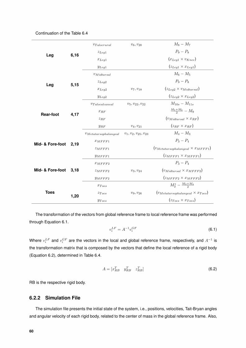
Figure 7.2: Muscle Force and Muscle Activation of the triceps surae obtained in the musculotendon model and inthe muscle model (contractile component represented by dash line with the correspondent muscle line color)
Figure 7.3: Muscle Force and Muscle Activation of the quadriceps femoris obtained in the musculotendon modeland in the muscle model (contractile component represented by dash line with the correspondent muscle line color)
66
Figure 7.4: Muscle Force and Muscle Activation of the hamstring obtained in the musculotendon model and in themuscle model (contractile component represented by dash line with the correspondent muscle line color)
Figure 7.5: Muscle Force and Muscle Activation of the ilipsoas obtained in the musculotendon model and in themuscle model (contractile component represented by dash line with the correspondent muscle line color)
67
Figure 7.6: Muscle Force and Muscle Activation of the gluteus maximus obtained in the musculotendon model andin the muscle model (contractile component represented by dash line with the correspondent muscle line color)
Figure 7.7: Muscle Force and Muscle Activation of the tibialis posterior obtained in the musculotendon model andin the muscle model (contractile component represented by dash line with the correspondente muscle line color)
68
Figure 7.8: Muscle Force and Muscle Activation of the tibialis anterior obtained in the musculotendon model and inthe muscle model (contractile component represented by dash line with the correspondent muscle line color)
The results obtained in both models must be compared to understand the influence of the tendon in
gait. The principal difference present is the presence of passive force in the muscle model. According
to the force-length muscle relationship this means that the muscle length is longer compared with the
isometric muscle length.
In the musculotendon model, the variation of tendon length enables the muscle to work at a more op-
timal velocity vM0 and length lM0 . When muscle working in this zone, the activation needed to developed
the force required will be lower than the present in the muscle model.
In Figure 7.2, where are represented the results of triceps surae significant differences are detected.
If the muscle force obtained with the musculotendon model were compared with the contractile muscle
force obtained (dash lines with the respective color) the differences are too small, which means that the
passive force is almost nonexistent. Otherwise, when analyze the results of the muscle model, although
the muscle force produce by those muscle are greater, most of them correspond to passive force. The
muscle is then working in a non-favorable zone, when it needs more activation to obtain the contractile
force to archive to the moment desired.
In relation to the quadriceps femoris (Figure 7.3), the same conclusion can be taken in relation to
rectus femoris. Otherwise, in vastus the muscle and the contractile force are practically equal. In this
case, a clearly conclusion about the influence of the tendon cannot be performed since the optimizer
give different weights to the muscle to produce extension of the knee.
In the hamstring (Figure 7.4), the tendon, according to the results, do not have influence. The muscle
force is practically equal to the contractile force with small and not influenced differences.
69
The two models present some different in the intensity of the muscle force during the cycle. The
mainly difference found is in the semimembranosus. At 20% of the gait, this muscle present a muscle
force much higher in the musculotendon model than in the muscle model. This value occurs when the
hip is extended and the right leg support all the body weight. In the muscle model, this force is exerted
by the gluteus maximus, as seen in Figure 7.6. Since those muscles are hip extensors, both must be
working as happen in the musculotendon model.
In Tibialis Posterior (Figure 7.7), a strong passive component was obtained in the muscle model.
A clearly evidence of the influence of the tendon is present in this muscle. Comparing the contractile
force and muscle activation of the muscle model to the musculotendon model, much more activation
was needed to realize the same movement, once the muscle is not work in the optimal zone.
Finally, in Tibialis Anterior (Figure 7.8), iliacus and Psoas (Figure 7.5), the influence of the tendon is
not remarkable.
To end the discussion of the gait analysis, the results obtained was compared to the literature. The
results obtained are very similar to the ones present to the work of Crowninshield and Brand (Crownin-
shield & Brand, 1981), mainly in the gait phases where are present activation and consequently, muscle
force.
7.2 Run Analysis
Running, like walking, is an activity characterized by a cycle which repeats over time. In this analyses
the cycle beginning and end with HS. Unlike what happen in gait cycle, running only is divided into a
support phase, when a foot is on the ground and a recovery phase in which both feet are off ground.
The results present in this work are referent to the support and recovery phase of the right limb.
This only represent 55% of the running cycle (Figure 7.9), once is not observable opposite heel strike
(OHS) and the final HS of the right limb. This happens due to absence of space in the Laboratory during
acquisition of running analysis, when the the remains phase of the cycle was out of the volume detection
of the cameras.
Figure 7.9: Scheme with different phases of Running Cycle
70
As happen in gait cycle, the stance phase consist in the period where the right limb is in contact with
the ground, and the swing phase where is not. Both phases are divided in different events, which name
are based on the movement on the foot.
The stance phase starts, in this case, with a heel contact and it is followed by a mid stance phase
(30%), when the right limb support all the body weight and occur the forward progressing of the body.
This phase ends with TO and the swing phase begins with double float, no foot is in contact with the
ground.
Through the results obtained (Figure 7.10 to Figure 7.16), high levels of muscle activation and con-
sequently the muscle forces are present in the stance phase, as expected. Between the 40% and 55%,
double float phase, there is a decrease of those levels. The description of the activity of the muscle and
the respective muscle force along the cycle will realize only for the results obtained by the musculotendon
model.
After the HS and before the mid stance phase occurs a period of absorption. In this period the body’s
center of mass decrease and its velocity decelerates horizontally (Hamner & Delp, 2010). Analyzing
Figure 7.11, Figure 7.14 and Figure 7.12 strong muscle activity is present in the knee (quadriceps
femoris) and hip extensors (gluteus maximus and hamstring). Quadriceps femoris are activated in this
period to prepare the limb for the ground contact and to absorb the shock of the impact. The hip
extensors, gluteus maximus and the hamstring, mainly the semimembranosus, also present high levels
of activations to contribute to the body support. The activation of these muscles, together with the triceps
surae, will provide the acceleration of the body vertically until the mid stance.
Forward propulsion of the body in this phase is provided initially by hip extensors discussed above,
and after mid stance by the ankle plantarflexors, soleus, gastrocnemius (GM, GL) (Figure 7.10) and
peroneus longus (Figure 7.15).
In the beginning of the swing phase, tibialis anterior (Figure 7.16), iliacus and psoas (Figure 7.13)
are activated to prepare the foot for the next HS, and to flex the hip joint, respectively.
During double float phase, occurs an increase activity of the hamstrings (Figure 7.12) to decelerate
the lower leg and foot and preparing to the new HS.
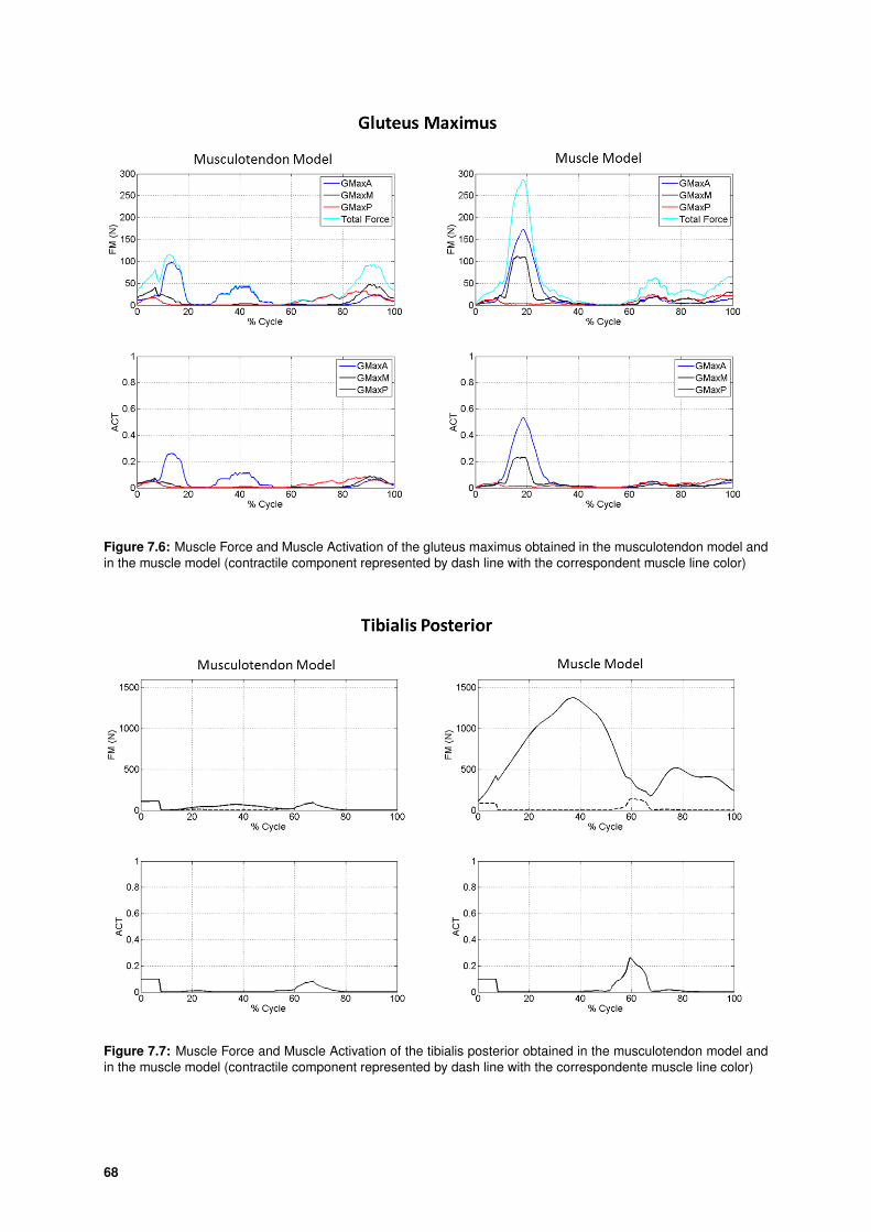
Comparing the two models, some differences are also found. Starting with the triceps surae (Figure
7.10), the presence of a tendon improves the results. The muscles work in optimal zone allowing the
production of more force with less activation. In the results of the muscle model, the muscle force are
mainly compose by a passive component and the muscle activation are at the same levels compare to
the other model, but the contractile force produce is almost zero. Also, the gastrocnemius, either the
medial or the lateral, should be active until the TO and not after as happen in the Muscle model. The
contraction of those muscles before the TO is very important to bring the body forward.
71
Figure 7.10: Muscle Force and Muscle Activation of the triceps surae obtained in the musculotendon model and inthe muscle model (contractile component represented by dash line with the correspondent muscle line color)
Figure 7.11: Muscle Force and Muscle Activation of the quadriceps femoris obtained in the musculotendon modeland in the muscle model (contractile component represented by dash line with the correspondent muscle line color)
72
Figure 7.12: Muscle Force and Muscle Activation of the hamstring obtained in the musculotendon model and in themuscle model (contractile component represented by dash line with the correspondent muscle line color)
Figure 7.13: Muscle Force and Muscle Activation of the ilipsoas obtained in the musculotendon model and in themuscle model (contractile component represented by dash line with the correspondent muscle line color)
73
Figure 7.14: Muscle Force and Muscle Activation of the gluteus maximus obtained in the musculotendon modeland in the muscle model (contractile component represented by dash line with the correspondent muscle line color)
Figure 7.15: Muscle Force and Muscle Activation of the tibialis posterior and peroneus longus obtained in the mus-culotendon model and in the muscle model (contractile component represented by dash line with the correspondentmuscle line color)
74
Figure 7.16: Muscle Force and Muscle Activation of the tibialis anterior obtained in the musculotendon model andin the muscle model (contractile component represented by dash line with the correspondent muscle line color)
As happen in gait analysis, in the quadriceps femoris (Figure 7.11) only the rectus femoris has
significant passive components, mainly in the double float phase. In vastus medialis and intermedius,
the influence of the tendon is verified. It is notable in Figure 7.11 that with lower values of muscle
activation, the muscle is producing more muscular force. Although in the results of the vastus lateralis
does not exist almost passive component, the change of the tendon length improve the results, once
only with the double of muscle activation, the muscle produce a muscle force six time more comparing
the two models.
Finally, the rectus femoris is more active when using musculotendon model. Since, in the stance
phase these muscles are responsible to absorb the force of impact it is expected a muscle force high.
In Hamstring (Figure 7.12) the same conclusions can be taken. In the beginning the swing phase, the
force developed by the semimembranosus is completely influence by the change of the tendon length.
The passive component is low, and the force developed is very high when analyzed the muscle activation
obtained. Analyzing, the double float phase, the something happens with the semitendinosus and with
biceps femoris long head.
Observing the result obtained for ilipsoas (Figure 7.13), the passive component is almost zero and it
is not evident the influence of the tendon. The same happens with tibialis anterior.
In gluteus maximus (Figure 7.14), only is notable the presence of the tendon in the posterior. Finally,
the tibialis posterior (Figure 7.15) where also the some conclusions can be taken.
Compared the results obtained with the ones presents in the Hamner and Delp work (Hamner &
Delp, 2010), correlation in the zone where the muscle are activated during the cycle are found.
75
7.3 Jump Analysis
Jumping is divided biomechanically into three phases: preparation, action and recovery (Bartlett,2007)
(Figure 7.17). The first one is characterize as the lowering phase, which positioning the body for the ac-
tion phase and stores elastic energy in the eccentrically contracting muscle. The action phase is featured
by a upper phase until feet leave the floor, where both knee joints extending or plantarflexing together.
The recovery phase involves the air and controlled landing, through, in the last one, eccentric contraction
of the leg muscles.
Figure 7.17: Scheme with different phases of Jumping Cycle
In the preparation phase, occur the flexion of the hip and knee and the dorsiflexion of the ankle. To
allow this movements the hamstrings (semimembranosus, semitendinosus and biceps femoris) (Figure
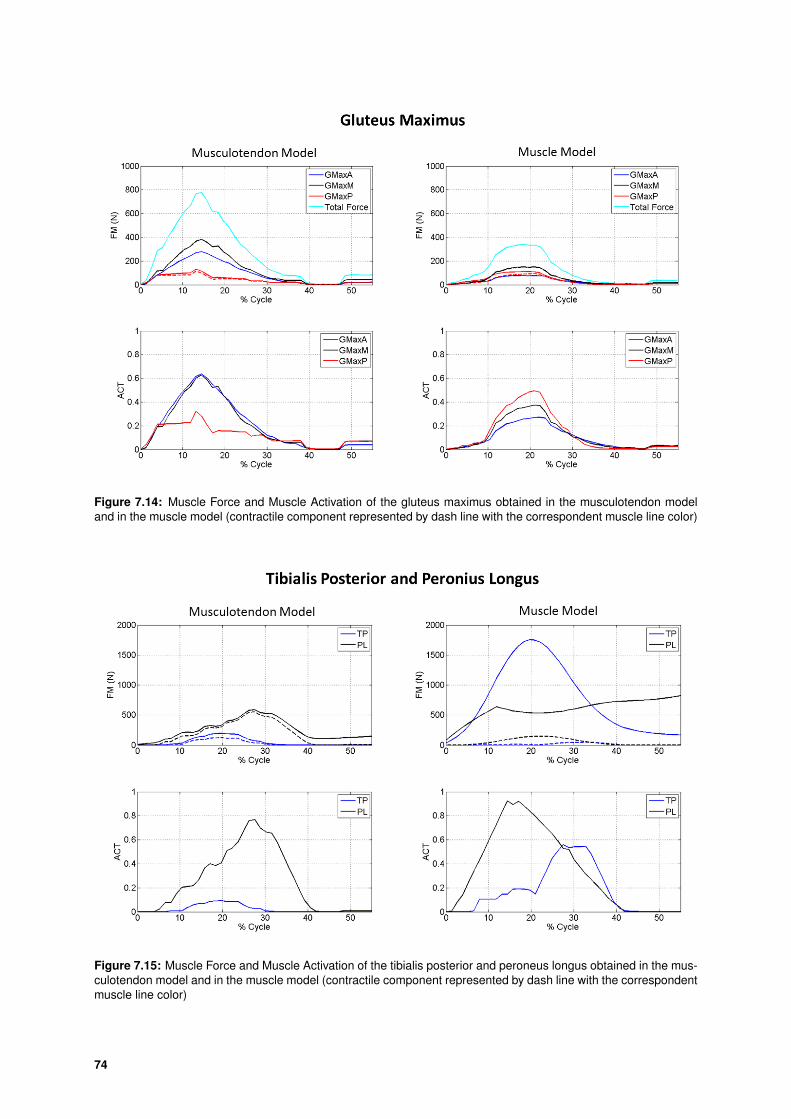
7.20), and the hip flexors, mainly rectus femoris (RF) (Figure 7.19), ilipsoas (Figure 7.21), contract.
The action phase involves the hip and knee extension and the ankle plantarflexion through contrac-
tion of the muscle responsible for that movement driving the body vertically upwards. Analyzing the
results obtained, the hip extensors (bicep femoris, semitendinosus, semimembranosus (Figure 7.20)
and gluteus maximus (Figure 7.22) present muscle activity and consequently muscle force that enable
the movement. The quadriceps femoris are activated to promote the knee extension and the gastrocne-
mius, soleus (Figure 7.18), peroneus longus, tibialis posterior (Figure 7.23) are also activated to enable
the plantarflexion.
In the air phase, the muscle activity observed is must lower than the remain cycle. In landing phase
(75% of cycle), a great activity is observed in quadriceps femoris (Figure 7.19) and gluteus maximus
(Figure 7.22) to stabilize knee and pelvis joints, respectively. The muscle force realize by the quadriceps
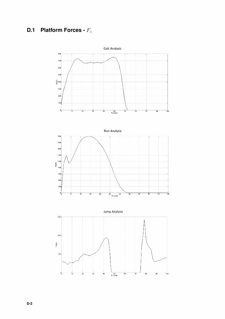
femoris (Figure 7.19) during landing is higher than in the impulse phase. In Annex D, (Jump analysis
figure), where the force in z direction realize in force platform is represented, it is possible to observed
that the force realize it conform the results observed.
The integration of the tendon in the model also influences the results in the jump but passive force
is now present in both models due to the type of movement. Analyzing the results obtained by the two
76
models, the same conclusions already taken in the previous section could be made for the triceps surae
(Figure 7.18), gluteus maximus (Figure 7.22), ilipsoas (Figure 7.21), tibialis posterior and peroneus
longus (Figure 7.23). The quadriceps femoris constitute the set of muscles that present a significant
passive component, but it do not influence the differences found in the two models in the contractile
force and muscle activation when compared.
The results obtained for the hamstring (Figure 7.20) feature many differences in order to be able to
conclude over the benefits of the tendon.
Finally, in tibialis anterior (Figure 7.24), once again, the integration of the tendon is not remarkable.
The activity of this muscle is much higher in the muscle model in the air phase. The excessive activity
present in the tibialis anterior using the muscle model it is to compensate the excessive passive compo-
nent that occurs in the plantarflexors, mainly the peroneus longus, in the same phase of the movement.
Taking into account the literature (Spagele et al, 1998), a correlation of the phases where the muscle
are activates is clearly present.
Figure 7.18: Muscle Force and Muscle Activation of the triceps surae obtained in the musculotendon model and inthe muscle model (contractile component represented by dash line with the correspondent muscle line color)
77
Figure 7.19: Muscle Force and Muscle Activation of the quadriceps femoris obtained in the musculotendon modeland in the muscle model (contractile component represented by dash line with the correspondent muscle line color)
Figure 7.20: Muscle Force and Muscle Activation of the hamstring obtained in the musculotendon model and in themuscle model (contractile component represented by dash line with the correspondent muscle line color)
78
Figure 7.21: Muscle Force and Muscle Activation of the ilipsoas obtained in the musculotendon model and in themuscle model (contractile component represented by dash line with the correspondent muscle line color)
Figure 7.22: Muscle Force and Muscle Activation of the gluteus maximus obtained in the musculotendon modeland in the muscle model (contractile component represented by dash line with the correspondent muscle line color)
79
Figure 7.23: Muscle Force and Muscle Activation of the tibialis posterior and peroneus longus obtained in the mus-culotendon model and in the muscle model (contractile component represented by dash line with the correspondentmuscle line color)
Figure 7.24: Muscle Force and Muscle Activation of the tibialis anterior obtained in the musculotendon model andin the muscle model (contractile component represented by dash line with the correspondent muscle line color)
80
7.4 Discussion
Analysing the results obtained in the three movements study, concludes that the importance of the
tendon depends on the muscle and on the type of movement. The presence of the tendon in triceps
surae and tibialis posterior interfere in the results in the gait, run and jump. Unlike what happens with
the tibialis anterior, the implementation of the musculotendon model is not remarkable. In ilipsoas and
quadriceps femoris, differences found are more significantly in jump than in gait or run.
Concluding, the use of model that includes the behavior of the tendon in the analysis of movement
is important in all type of movement. With the implementation of the musculotendon model developed in
this thesis, the results obtained are physiologically more real even when the presence of the tendon is
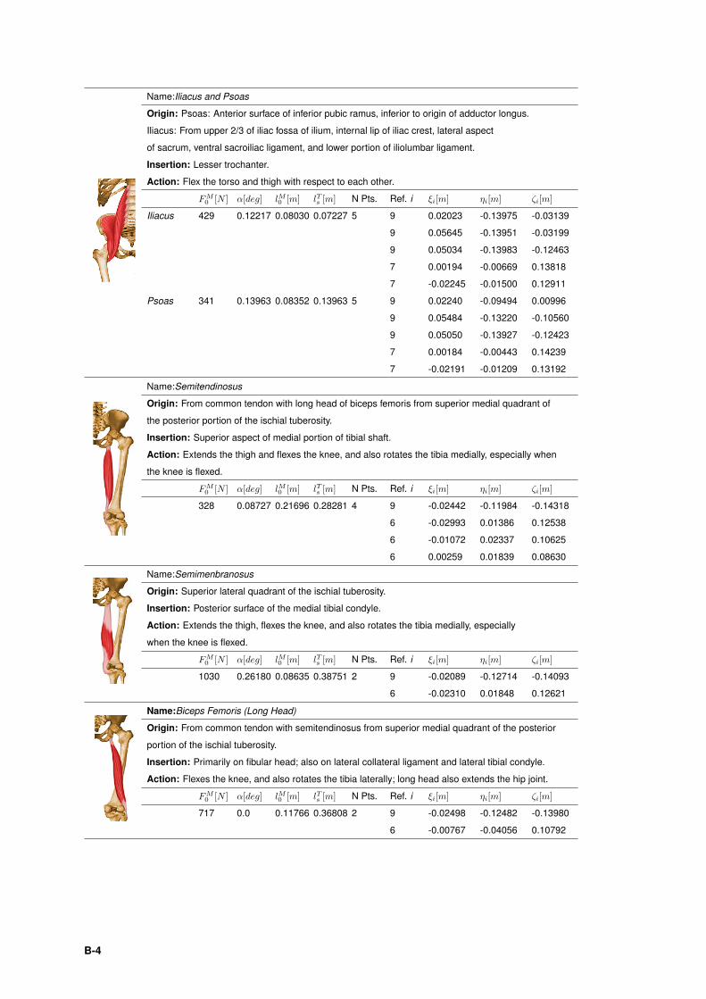
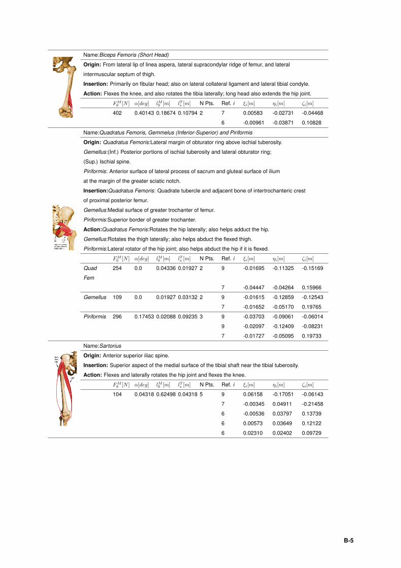
Table B.1: Properties of the muscle of the lower extremity of the Biomechanical model (Silva,2003). The values ofthe origin, insertion and via points are referent to a right lower extremity. The value of the left lower limb must to bescaled with the respective length and are symmetrical in y-direction.
Name:Gluteus Medius
Origin: Dorsal ilium inferior to iliac crest
Insertion: Lateral and Superior surfaces of greater trochanter
Action: Major abductor of high; anterior fibers to rotate hip medially;
posterior fibers help to rotate hip laterally
FM0 [N ] α[rad] lM0 [m] lTs [m] N Pts. Ref. i ξi[m] ηi[m] ζi[m]