394


Copyright
by
MEHMET BARIS DARENDELI
2001


DEVELOPMENT OF A NEW FAMILY OF NORMALIZED
MODULUS REDUCTION AND MATERIAL DAMPING
CURVES
by
MEHMET BARIS DARENDELI, B.S., M.S.
DISSERTATION
Presented to the Faculty of the Graduate School of
The University of Texas at Austin
in Partial Fulfillment
of the Requirements
for the Degree of
DOCTOR OF PHILOSOPHY
The University of Texas at Austin
August, 2001

Dedicated
To
My Parents,
My Wife and My Daughter

v
Acknowledgements
I would like to thank my supervising professor Dr. Kenneth H. Stokoe, II
for his guidance and support through the course of this study. His passion and
enthusiasm in his work has always inspired me. Our stimulating conversations
have made this study enjoyable.
Dr. Robert B. Gilbert’s assistance and guidance, which have made this
dissertation possible, is gratefully acknowledged. Besides his valuable input to
this work, he has influenced my perception of science and engineering with his
lectures on decision, risk and reliability.
I would also like to thank my dissertation committee members Dr. Jose M.
Roesset, Dr. Ellen M. Rathje, Dr. Alan F. Rauch and Dr. Mark F. Hamilton for
reviewing this dissertation in such a limited time frame and for their valuable
contributions to this work. Thanks are also extended to the rest of the former and
current geotechnical engineering faculty, Dr. Roy E. Olson, Dr. David E. Daniel,
and Dr. Stephen G. Wright for their lectures that broadened my knowledge.
The support from the California Department of Transportation, the
National Science Foundation, the Electric Power Research Institute, and Pacific
Gas and Electric Company is gratefully acknowledged for funding various stages
of the ROSRINE project. I would also like to acknowledge the contributions of
the National Institute of Standards and Technology, the United States Geological
Survey, the Department of Energy, the Westinghouse Savannah River
Corporation, Kajima Corporation, Geovision, Agbabian Associates, Fugro, Inc.,
Earth Mechanics, Inc., S&ME, Inc. in funding the research projects the results of

vi
which are utilized in this study. Encouragement and guidance from Dr. Clifford
Roblee, Dr. John Schneider, Dr. Walter Silva, Dr. Robert Pyke, Dr. Robert
Nigbor, Dr. David Boore, Prof. Mladen Vucetic and Dr. Richard Lee, who took
part in these research projects, are appreciated.
Thanks to my best friend Cem Akguner for always being there whenever I
needed him, to Dr. Brent L. Rosenblad for trying to teach me how to bat
whenever we overworked, to Dr. Ahmet Yakut for our stimulating card plays and
arguments regarding them that lasted for hours, and to Baris Binici for each and
every five minute coffee break at 100oF. You have kept me sane (although
everyone reading this paragraph will question it a little) for the past seven years.
I would also like to thank the former and current graduate students that I
have worked side by side. I enjoyed each and every day and night that I worked
together with Dr. James A. Bay, Dr. Seon-Keun Hwang, Farn-Yuh Menq, Brian
Moulin, Celestino Valle and Nicola Chiara. Thanks are also extended to other
graduate students of whom I had the pleasure of making acquaintance; Dr. Eric
Liedtke, Dr. Mike Kalinski, Jeffrey Lee, Paul Axtell, Jiun Chen, Cem Topkaya
and many others that I unfortunately omitted. I would also like to thank Teresa
Tice-Boggs and Alicia Zapata for their administrative support, and Frank Wise,
Gonzalo Zapata, Max Trevino and Paul Walters for their technical assistance over
the years.

vii
DEVELOPMENT OF A NEW FAMILY OF NORMALIZED
MODULUS REDUCTION AND MATERIAL DAMPING
CURVES
Publication No._____________
Mehmet Baris Darendeli, Ph.D.
The University of Texas at Austin, 2001
Supervisor: Kenneth H. Stokoe, II
As part of various research projects [including the SRS (Savannah River Site)
Project AA891070, EPRI (Electric Power Research Institute) Project 3302, and
ROSRINE (Resolution of Site Response Issues from the Northridge Earthquake)
Project], numerous geotechnical sites were drilled and sampled. Intact soil
samples over a depth range of several hundred meters were recovered from 20 of
these sites. These soil samples were tested in the laboratory at The University of
Texas at Austin (UTA) to characterize the materials dynamically. The presence of
a database accumulated from testing these intact specimens motivated a re-
evaluation of empirical curves employed in the state of practice. The weaknesses
of empirical curves reported in the literature were identified and the necessity of
viii
developing an improved set of empirical curves was recognized. This study
focused on developing the empirical framework that can be used to generate
normalized modulus reduction and material damping curves. This framework is
composed of simple equations, which incorporate the key parameters that control
nonlinear soil behavior. The data collected over the past decade at The University
of Texas at Austin are statistically analyzed using First-order, Second-moment
Bayesian Method (FSBM). The effects of various parameters (such as confining
pressure and soil plasticity) on dynamic soil properties are evaluated and
quantified within this framework. One of the most important aspects of this study
is estimating not only the mean values of the empirical curves but also estimating
the uncertainty associated with these values. This study provides the opportunity
to handle uncertainty in the empirical estimates of dynamic soil properties within
the probabilistic seismic hazard analysis framework. A refinement in site-specific
probabilistic seismic hazard assessment is expected to materialize in the near
future by incorporating the results of this study into the state of practice.

ix
TABLE OF CONTENTS
LIST OF TABLES ...............................................................................................xiii
LIST OF FIGURES............................................................................................xviii
CHAPTER 1 INTRODUCTION........................................................................ 1 1.1 Background ........................................................................................... 1 1.2 Dynamic Soil Properties........................................................................ 4 1.3 Ground Response Analysis ................................................................... 8 1.4 Objectives of Research........................................................................ 10 1.5 Organization of Dissertation ............................................................... 11
CHAPTER 2 LABORATORY TESTING EQUIPMENT............................... 13 2.1 Introduction ......................................................................................... 13 2.2 Combined Resonant Column and Torsional Shear Equipment........... 14 2.3 Torsional Resonant Column Test ........................................................ 16 2.4 Cyclic Torsional Shear Test ................................................................ 21 2.5 Summary ............................................................................................. 22
CHAPTER 3 PHYSICAL PROPERTIES OF TEST SPECIMENS ................ 23 3.1 Introduction ......................................................................................... 23 3.2 Undisturbed Soil Specimens from Northern California...................... 25 3.3 Undisturbed Soil Specimens from Southern California...................... 29 3.4 Undisturbed Soil Specimens from South Carolina ............................. 35 3.5 Undisturbed Soil Specimens from Lotung, Taiwan ............................ 38 3.6 Overview of The Database .................................................................. 39 3.7 Summary ............................................................................................. 53
CHAPTER 4 OBSERVED TRENDS IN DYNAMIC SOIL PROPERTIES .. 54 4.1 Introduction ......................................................................................... 54 4.2 Background ......................................................................................... 54 4.3 Nonlinear Dynamic Soil Properties..................................................... 56

x
4.4 Effect of Duration of Confinement on Small-Strain Dynamic Soil Properties............................................................................................. 59
4.5 Effect of Effective Confining Pressure ............................................... 61 4.6 Effect of Overconsolidation Ratio....................................................... 70 4.7 Effect of Number of Cycles ................................................................ 74 4.8 Effect of Loading Frequency............................................................... 76 4.9 Effect of Soil Type .............................................................................. 81 4.10 Effect of Sample Disturbance ............................................................. 90 4.11 Summary ........................................................................................... 104
CHAPTER 5 EMPIRICAL RELATIONSHIPS ............................................ 107 5.1 Introduction ....................................................................................... 107 5.2 Hardin and Drnevich (1972) Design Equations ................................ 107 5.3 Empirical Relationships .................................................................... 113 5.4 Summary ........................................................................................... 129
CHAPTER 6 PROPOSED SOIL MODEL .................................................... 131 6.1 Introduction ....................................................................................... 131 6.2 Normalized Modulus Reduction Curve............................................. 132 6.3 Nonlinear Material Damping Curve.................................................. 134 6.4 Parametric Study of The Soil Model................................................. 147 6.5 Summary ........................................................................................... 152
CHAPTER 7 STATISTICAL ANALYSIS OF COLLECTED DATA USING FIRST-ORDER, SECOND-MOMENT BAYESIAN METHOD 154 7.1 Introduction ....................................................................................... 154 7.2 Bayesian Approach ........................................................................... 155 7.3 First-Order, Second-Moment Bayesian Method ............................... 164 7.4 Form of Proposed Equations ............................................................. 172 7.5 Summary ........................................................................................... 179

xi
CHAPTER 8 STATISTICAL ANALYSIS OF THE RCTS DATA.............. 180 8.1 Introduction ....................................................................................... 180 8.2 Analysis of Subsets of The Data ....................................................... 184 8.3 Analysis of All Credible Data ........................................................... 212 8.4 Summary ........................................................................................... 217
CHAPTER 9 PREDICTING NONLINEAR SOIL BEHAVIOR USING THE CALIBRATED MODEL................................................................... 220 9.1 Introduction ....................................................................................... 220 9.2 Calculation of Reference Strain, Curvature Coefficient, Small-
Strain Material Damping Ratio and the Scaling Coefficient............. 221 9.3 Estimation of Normalized Modulus Reduction and Material
Damping Curves................................................................................ 224 9.4 Effect of Overconsolidation Ratio, Loading Frequency and
Number of Loading Cycles on Nonlinear Soil Behavior .................. 228 9.5 Effect of Confining Pressure on Nonlinear Soil Behavior ................ 234 9.6 Effect of Soil Type on Nonlinear Soil Behavior ............................... 238 9.7 Effects of Confining Pressure and Soil Type on Stress-Strain
Curves................................................................................................ 242 9.8 Summary ........................................................................................... 248
CHAPTER 10 RECOMMENDED NORMALIZED MODULUS REDUCTION AND MATERIAL DAMPING CURVES ......................... 249 10.1 Introduction ....................................................................................... 249 10.2 Effect of PI at a Given Mean Effective Stress .................................. 250 10.3 Effect of Mean Effective Stress on a Soil with Given Plasticity ...... 250 10.4 Impact of Utilizing the Recommended Curves on Earthquake
Response Predictions of Deep Sites .................................................. 250 10.5 Summary ........................................................................................... 272
CHAPTER 11 UNCERTAINTY ASSOCIATED WITH THE MODEL PREDICTIONS.......................................................................................... 273 11.1 Introduction ....................................................................................... 273 11.2 Uncertainty in Nonlinear Soil Behavior............................................ 273

xii
11.3 Uncertainty in Predicted Ground Motions Due to the Uncertainty in Nonlinear Soil Behavior................................................................ 284
11.4 Summary ........................................................................................... 295
CHAPTER 12 SUMMARY AND CONCLUSIONS....................................... 296 12.1 Summary ........................................................................................... 296 12.2 Conclusions ....................................................................................... 301
APPENDIX A ..................................................................................................... 303
APPENDIX B ..................................................................................................... 306
APPENDIX C ..................................................................................................... 311
APPENDIX D ..................................................................................................... 338
REFERENCES.................................................................................................... 357
VITA ................................................................................................................... 363

xiii
LIST OF TABLES
Table 3.1 Physical properties of soils recovered from Oakland Outer Harbor and test pressures (Hwang, 1997) ..................................... 24
Table 3.2 Physical properties of soils recovered from Treasure Island and test pressures (Hwang and Stokoe, 1993b; and Hwang, 1997).............................................................................................. 25
Table 3.3 Physical properties of soils recovered from San Francisco Airport and test pressures (Hwang, 1997)..................................... 27
Table 3.4 Physical properties of soils recovered from Gilroy and test pressures (Hwang and Stokoe, 1993c; Hwang, 1997; and Stokoe et al., 2001)........................................................................ 27
Table 3.5 Physical properties of soils recovered from Garner Valley and test pressures (Stokoe and Darendeli, 1998) .......................... 28
Table 3.6 Physical properties of soils recovered from San Francisco-Oakland Bay Bridge Site and test pressures (Stokoe et al., 1998d)............................................................................................ 28
Table 3.7 Physical properties of soils recovered from Corralitos and test pressures (Stokoe et al., 2001) ................................................ 28
Table 3.8 Physical properties of soils recovered from Borrego and test pressures (Hwang, 1997)............................................................... 32
Table 3.9 Physical properties of soils recovered from Arleta and test pressures (Darendeli and Stokoe, 1997; and Darendeli, 1997) ..... 32
Table 3.10 Physical properties of soils recovered from Kagel and test pressures (Darendeli and Stokoe, 1997; and Darendeli, 1997) ..... 32
Table 3.11 Physical properties of soils recovered from La Cienega and test pressures (Darendeli and Stokoe, 1997; Darendeli, 1997; and Stokoe et al., 1998e) ............................................................... 33
Table 3.12 Physical properties of soils recovered from Newhall and test pressures (Darendeli and Stokoe, 1997; and Darendeli, 1997) ..... 33
xiv
Table 3.13 Physical properties of soils recovered from Sepulveda V.A. Hospital and test pressures (Darendeli and Stokoe, 1997; and Darendeli, 1997)............................................................................ 34
Table 3.14 Physical properties of soils recovered from Potrero Canyon and test pressures (Stokoe et al., 1998e) ....................................... 34
Table 3.15 Physical properties of soils recovered from Rinaldi Receiving Station and test pressures (Stokoe et al., 1998e). .......................... 34
Table 3.16 Physical properties of soils recovered from North Palm Springs and test pressures (Stokoe et al., 2001) ............................ 35
Table 3.17 Physical properties of soils recovered from Imperial Valley College and test pressures (Stokoe et al., 2001)............................ 35
Table 3.18 Physical properties of soils recovered from Savannah River Site and test pressures (Hwang, 1997; and Stokoe et al., 1998a)............................................................................................ 37
Table 3.19 Physical properties of soils recovered from Daniel Island and test pressures (Stokoe et al., 1998b). ............................................. 37
Table 3.20 Physical properties of soils recovered from Lotung site and test pressures (Hwang and Stokoe, 1993a; and Hwang, 1997) ..... 39
Table 3.21 Distribution of soil samples according to the sample depth in each geographic region.................................................................. 41
Table 3.22 Distribution of collected according to the isotropic confining pressure in each geographic region ............................................... 42
Table 3.23 Distribution of soil samples according to the Unified Soil Classification System (USCS) designation and sample depth ...... 44
Table 4.1 Parameters that control nonlinear soil behavior and their relative importance in terms of affecting normalized modulus reduction and material damping curves based on general trends observed during the course of this study .......................... 105
Table 5.1 Parameters that control nonlinear soil behavior and their relative importance in terms of affecting shear modulus and material damping (Hardin and Drnevich, 1972b) ....................... 108
xv
Table 7.1 Prior information provided in the discrete example.................... 160
Table 7.2 Prior information regarding the model parameters in the FSBM example............................................................................ 165
Table 7.3 Prior covariance structure of the model parameters in the FSBM example............................................................................ 165
Table 7.4 Data used to calibrate the model parameters in the FSBM example ....................................................................................... 166
Table 7.5 Comparison of the prior and posterior information regarding the model parameters in the FSBM example .............................. 169
Table 7.6 Posterior covariance structure of the model parameters in the FSBM example............................................................................ 170
Table 7.7 Posterior covariance structure of the model parameters in the FSBM example............................................................................ 171
Table 8.1 Distribution of specimens with soil type and geographic location ........................................................................................ 181
Table 8.2 Distribution of specimens by soil group and geographic location ........................................................................................ 181
Table 8.3 Distribution of specimens with soil type and geographic location for the updated database ................................................ 182
Table 8.4 Distribution of specimens by soil group and geographic location for the updated database ................................................ 183
Table 8.5 Prior mean values and variances of the model parameters ......... 185
Table 8.6 Updated mean values and variances of the model parameters for the soils from Northern California......................................... 186
Table 8.7 Updated mean values and variances of the model parameters for the soils from Southern California......................................... 191
Table 8.8 Updated mean values and variances of the model parameters for the soils from South Carolina ................................................ 194
xvi
Table 8.9 Updated mean values and variances of the model parameters for the South Carolina soil groups affected by change in the contents of the database............................................................... 198
Table 8.10 Updated mean values and variances of the model parameters for the soils from Lotung, Taiwan............................................... 200
Table 8.11 Updated mean values and variances of the model parameters for the four soil groups ................................................................ 207
Table 8.12 Comparison of the prior and updated mean values and variances of the model parameters for all the credible data ........ 214
Table 8.13 Covariance structure of the updated model parameters for all the credible data .......................................................................... 218
Table 10.1 Effect of PI on normalized modulus reduction curve: σo’ = 0.25 atm....................................................................................... 252
Table 10.2 Effect of PI on material damping curve: σo’ = 0.25 atm............. 252
Table 10.3 Effect of PI on normalized modulus reduction curve: σo’ = 1.0 atm......................................................................................... 254
Table 10.4 Effect of PI on material damping curve: σo’ = 1.0 atm............... 254
Table 10.5 Effect of PI on normalized modulus reduction curve: σo’ = 4.0 atm......................................................................................... 256
Table 10.6 Effect of PI on material damping curve: σo’ = 4.0 atm............... 256
Table 10.7 Effect of PI on normalized modulus reduction curve: σo’ = 16 atm............................................................................................... 258
Table 10.8 Effect of PI on material damping curve: σo’ = 16 atm................ 258
Table 10.9 Effect of σo’ on normalized modulus reduction curve: PI = 0 %.................................................................................................. 260
Table 10.10 Effect of σo’ on material damping curve: PI = 0 % ................... 260

xvii
Table 10.11 Effect of σo’ on normalized modulus reduction curve: PI = 15 %............................................................................................. 262
Table 10.12 Effect of σo’ on material damping curve: PI = 15 % ................. 262
Table 10.13 Effect of σo’ on normalized modulus reduction curve: PI = 30 %............................................................................................. 264
Table 10.14 Effect of σo’ on material damping curve: PI = 30 % ................. 264
Table 10.15 Effect of σo’ on normalized modulus reduction curve: PI = 50 %............................................................................................. 266
Table 10.16 Effect of σo’ on material damping curve: PI = 50 % ................. 266
Table 10.17 Effect of σo’ on normalized modulus reduction curve: PI = 100 %........................................................................................... 268
Table 10.18 Effect of σo’ on material damping curve: PI = 100 % ............... 268
Table 11.1 Predicted mean values and standard deviations accounting for uncertainty in the values of model parameters and variability due to modeled uncertainty ......................................................... 275
Table 11.2 Predicted covariance structure accounting for uncertainty in the values of model parameters and variability due to modeled uncertainty .................................................................... 276
Table 11.3 Predicted mean values and standard deviations accounting only for variability due to modeled uncertainty .......................... 277
Table 11.4 Predicted covariance structure accounting only for variability due to modeled uncertainty ......................................................... 278
Table 12.1 Parameters that control nonlinear soil behavior and their relative importance in terms of affecting normalized modulus reduction and material damping curves based on general trends observed during the course of this study .......................... 297
xviii
LIST OF FIGURES
Figure 1.1 Evaluation of ground motion at a geotechnical site based on vertically propagating shear waves between the bedrock and ground surface ................................................................................. 2
Figure 1.2 Fourier amplitude of (a) the ground motion as a result of (b) the bedrock motion at the geotechnical site shown in Figure 1.1.................................................................................................... 3
Figure 1.3 Representation of a soil deposit in terms of dynamic soil properties in geotechnical earthquake engineering ......................... 4
Figure 1.4 Nonlinear stress-strain curve of soils and variation of secant shear modulus with shearing strain amplitude ................................ 5
Figure 1.5 Estimation of shear modulus and material damping ratio during cyclic loading....................................................................... 6
Figure 1.6 (a) Nonlinear shear modulus and (b) normalized modulus reduction curves .............................................................................. 7
Figure 1.7 Nonlinear material damping ratio curve.......................................... 7
Figure 1.8 Field curves representing nonlinear soil behavior........................... 9
Figure 2.1 Simplified diagram of the RCTS device (from Stokoe et al., 1999).............................................................................................. 14
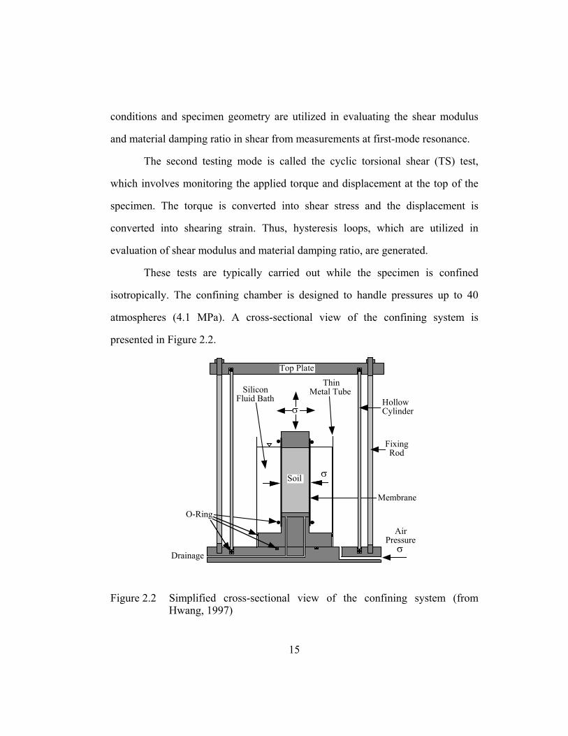
Figure 2.2 Simplified cross-sectional view of the confining system (from Hwang, 1997) ...................................................................... 15
Figure 2.3 General Configuration of RCTS Equipment (after Hwang, 1997).............................................................................................. 17
Figure 2.4 Frequency response curve measured in the RC test (from Stokoe et al., 1999)........................................................................ 18
Figure 2.5 Material damping measurement in the RC test using the half-power bandwidth (from Stokoe et al., 1999)................................. 18
xix
Figure 2.6 Material damping measurement in the RC test using the free-vibration decay curve (from Stokoe et al., 1999).......................... 19
Figure 2.7 Calculation of shear modulus and material damping ratio in the TS test...................................................................................... 21
Figure 3.1 Map of Northern California showing the locations of the geotechnical sites in this area ........................................................ 26
Figure 3.2 Map of Southern California showing the locations of the three geotechnical sites outside the Los Angeles area .................. 30
Figure 3.3 Map of Los Angeles showing the locations of the seven geotechnical sites in this area ........................................................ 31
Figure 3.4 Map of South Carolina showing the locations of the geotechnical sites in this area ........................................................ 36
Figure 3.5 Map of Taiwan showing the location of Lotung site .................... 38
Figure 3.6 Distribution of soil samples with geographic region .................... 40
Figure 3.7 Distribution of the number of geotechnical sites with geographic region.......................................................................... 40
Figure 3.8 Distribution of soil samples according to the sample depth.......... 41
Figure 3.9 Distribution of confining pressures at which nonlinear measurements were performed...................................................... 42
Figure 3.10 Distribution of soil samples according to soil type as classified by the Unified Soil Classification System (USCS)....... 43
Figure 3.11 Distribution of soil samples according to soil plasticity in terms of the plasticity index, PI..................................................... 44
Figure 3.12 Distribution of soil samples according to total unit weight .......... 46
Figure 3.13 Distribution of soil samples according to dry unit weight ............ 46
Figure 3.14 Distribution of soil samples according to water content ............... 47
Figure 3.15 Distribution of soil samples according to void ratio ..................... 47
xx
Figure 3.16 Variation of dry unit weight with depth of (a) fine grained and (b) coarse grained soils included in this study........................ 48
Figure 3.17 Variation of water content with depth of (a) fine grained and (b) coarse grained soils included in this study .............................. 49
Figure 3.18 Variation of void ratio with depth of (a) fine grained and (b) coarse grained soils included in this study .................................... 50
Figure 3.19 Distribution of soil samples according to estimated overconsolidation ratio.................................................................. 51
Figure 3.20 Variation of estimated overconsolidation ratio with depth of (a) fine grained and (b) coarse grained soils included in this study .............................................................................................. 52
Figure 4.1 Linear elastic, nonlinear elastic and plastic strain ranges on (a) normalized modulus reduction and (b) material damping curves ............................................................................................ 57
Figure 4.2 Variation of (a) low-amplitude shear modulus, (b) low-amplitude material damping ratio, and (c) void ratio with magnitude and duration of isotropic confining pressure............... 60
Figure 4.3 Variation of (a) low-amplitude shear modulus, (b) low-amplitude material damping ratio, and (c) void ratio with effective isotropic confining pressure ........................................... 62
Figure 4.4 The effect of confining pressure on the variation of (a) shear modulus, (b) normalized shear modulus, and (c) material damping ratio with shearing strain amplitude as measured in the torsional resonant column ....................................................... 65
Figure 4.5 The effect of confining pressure on normalized modulus reduction curve (a) for soils with moderate plasticity, and (b) for non-plastic soils evaluated as part of the ROSRINE study (after Stokoe et al., 1999) .............................................................. 67
Figure 4.6 The effect of confining pressure on (a) normalized modulus reduction and (b) material damping curves of silty sands evaluated as part of the ROSRINE study (after Darendeli et al., 2001)........................................................................................ 68
xxi
Figure 4.7 Impact on nonlinear site response of accounting for the effect of confining pressure on dynamic soil properties (after Darendeli et al., 2001) ................................................................... 70
Figure 4.8 The effect of overconsolidation ratio on the variation of (a) shear modulus, (b) material damping ratio, and (c) void ratio with effective isotropic confining pressure as measured in the torsional resonant column ............................................................. 71
Figure 4.9 The effect of overconsolidation ratio on the variation of (a) shear modulus, (b) normalized shear modulus, and (c) material damping ratio with shearing strain amplitude as measured in the torsional resonant column ................................... 72
Figure 4.10 The effect of number of loading cycles on the variation of (a) shear modulus, (b) normalized shear modulus, and (c) material damping ratio with shearing strain amplitude as determined in the combined RCTS testing ................................... 75
Figure 4.11 The effect of loading frequency on (a) low-amplitude shear modulus, and (b) low-amplitude material damping ratio as determined in the combined RCTS testing ................................... 77
Figure 4.12 Comparison of the effect of loading frequency on low-amplitude shear modulus and low-amplitude material damping ratio (from Stokoe and Santamarina, 2000) ................... 78
Figure 4.13 The effect of loading frequency on the variation of (a) shear modulus, (b) normalized shear modulus, and (c) material damping ratio with shearing strain amplitude as determined in the combined RCTS testing ...................................................... 80
Figure 4.14 The effect of soil type on the variation of (a) low-amplitude shear modulus, and (b) low-amplitude material damping ratio with effective isotropic confining pressure as determined in the combined RCTS testing........................................................... 82
Figure 4.15 The effect of soil type on the variation of low-amplitude shear modulus with loading frequency as determined in the combined RCTS testing ................................................................ 84
xxii
Figure 4.16 The effect of soil type on the variation of low-amplitude material damping ratio with loading frequency as determined in the combined RCTS testing ...................................................... 85
Figure 4.17 The effect of soil type on the normalized modulus reduction curve as measured in the torsional resonant column..................... 86
Figure 4.18 The effect of soil type on the material damping curve determined at (a) N ~ 1000 cycles, (b) N = 1 cycle, and (c) N = 10 cycles from combined RCTS testing .................................... 87
Figure 4.19 The effect of soil type on normalized modulus reduction and material damping curves (after Stokoe et al., 1999) ..................... 88
Figure 4.20 Comparison of field and laboratory measurements of shear wave velocity at the La Cienega site in the ROSRINE project..... 91
Figure 4.21 Variation of sampling disturbance expressed in terms of Vs,
lab/Vs, field and Gmax, lab/Gmax, field with the in-situ shear wave velocity .......................................................................................... 93
Figure 4.22 Comparison of laboratory and field measurements of small strain material damping ratio (from Stokoe et al., 1999) .............. 95
Figure 4.23 Comparison of nonlinear soil properties back-calculated from the free-field downhole accelerations with the laboratory measurements (from Zeghal et al., 1995)...................................... 96
Figure 4.24 Comparison of the variation of (a) low-amplitude shear modulus, (b) low-amplitude material damping ratio, and (c) void ratio with effective isotropic confining pressure of intact (undisturbed) and reconstituted (remolded) specimens ................ 99
Figure 4.25 Comparison of the variation of (a) shear modulus, (b) normalized shear modulus, and (c) material damping ratio with shearing strain of intact (undisturbed) and reconstituted (remolded) specimens ................................................................. 100
Figure 4.26 Comparison of the variation of (a) shear modulus, (b) normalized shear modulus, and (c) material damping ratio with shearing strain measured using various equipment on companion soil samples (from Stokoe et al., 1999) .................... 102

xxiii
Figure 5.1 Hyperbolic soil model proposed by Hardin and Drnevich (1972b) ........................................................................................ 110
Figure 5.2 The normalized modulus reduction and material damping curves estimated based on the hyperbolic model ........................ 112
Figure 5.3 The effect of confining pressure on normalized modulus reduction curve for Toyoura Sand (Iwasaki et al., 1978)............ 114
Figure 5.4 The effect of confining pressure on (a) normalized modulus reduction, and (b) material damping curves for Toyoura Sand (Kokusho, 1980).......................................................................... 115
Figure 5.5 The effect of confining pressure on (a) normalized modulus reduction, and (b) material damping curves for non-plastic soils (Ni, 1987) ............................................................................ 116
Figure 5.6 Empirical (a) normalized modulus reduction, and (b) material damping curves proposed by Seed et al. (1986).......................... 118
Figure 5.7 Empirical (a) normalized modulus reduction, and (b) material damping curves proposed by Sun et al. (1988) for soils with plasticity ...................................................................................... 119
Figure 5.8 Empirical (a) normalized modulus reduction, and (b) material damping curves proposed by Idriss (1990) ................................. 121
Figure 5.9 Empirical (a) normalized modulus reduction, and (b) material damping curves proposed by Vucetic and Dobry (1991)............ 122
Figure 5.10 The effect of confining pressure on (a) normalized modulus reduction, and (b) material damping curves for non-plastic soils (Ishibashi and Zhang, 1993) ............................................... 124
Figure 5.11 Empirical (a) normalized modulus reduction, and (b) material damping curves proposed by Ishibashi and Zhang (1993).......... 125
Figure 5.12 Variation in empirical (a) normalized modulus reduction, and (b) material damping curves with depth (EPRI, 1993c).............. 127
Figure 5.13 Variation in empirical (a) normalized modulus reduction, and (b) material damping curves with soil type (EPRI, 1993c)......... 128
xxiv
Figure 6.1 Normalized modulus reduction curve (of a silty sand at 1 atm effective confining pressure) represented using a modified hyperbolic model......................................................................... 133
Figure 6.2 Stress-strain curve (of a silty sand at 1 atm effective confining pressure) estimated based on a modified reference strain model ................................................................................. 135
Figure 6.3 Hysteresis loop estimated by modeling stress-strain reversals for two-way cyclic loading according to Masing behavior......... 137
Figure 6.4 Calculation of damping ratio utilizing a hysteresis loop............. 138
Figure 6.5 Variations of c1, c2 and c3 with curvature coefficient, a.............. 141
Figure 6.6 Damping curve estimated based on Masing behavior................. 143
Figure 6.7 Effect of high-amplitude cycling on low-amplitude shear modulus and material damping ratio (from Stokoe and Lodde, 1978) ............................................................................... 144
Figure 6.8 Comparison of the variation in F with shearing strain for different values of p..................................................................... 145
Figure 6.9 (a) Damping curve estimated based on Masing behavior, (b) adjusted curve using the scaling coefficient, and (c) shifted curve using the small-strain material damping ratio ................... 146
Figure 6.10 Effect of reference strain on (a) normalized modulus reduction, (b) stress-strain, and (c) material damping curves ..... 148
Figure 6.11 Effect of the curvature coefficient on the normalized modulus reduction curve............................................................................ 149
Figure 6.12 Effect of the curvature coefficient on the stress-strain curve (a) at small and intermediate strains, and (b) at high strains....... 149
Figure 6.13 Effect of the curvature coefficient on the material damping curve ............................................................................................ 150
Figure 6.14 Effect of Dmin on the material damping curve............................. 151
Figure 6.15 The effect of scaling coefficient on material damping curve...... 152

xxv
Figure 7.1 Prior probability mass function for the discrete example ........... 159
Figure 7.2 Posterior probability mass function for the discrete example ..... 161
Figure 7.3 Imaginary correlation between model parameters upon updating prior information based on limited number of observations................................................................................. 170
Figure 7.4 Variation of standard deviation with normalized shear modulus ....................................................................................... 176
Figure 7.5 Standard deviation modeled for normalized modulus reduction curve............................................................................ 177
Figure 7.6 Variation of standard deviation with material damping ratio ..... 178
Figure 7.7 Standard deviation modeled for material damping curve ........... 178
Figure 8.1 Comparisons of the measured and predicted values of (a) normalized modulus and (b) material damping ratio for “clean” sands from Northern California...................................... 188
Figure 8.2 Comparisons of the measured and predicted values of (a) normalized modulus and (b) material damping ratio for sands with high fines content from Northern California....................... 188
Figure 8.3 Comparisons of the measured and predicted values of (a) normalized modulus and (b) material damping ratio for silts from Northern California ............................................................ 189
Figure 8.4 Comparisons of the measured and predicted values of (a) normalized modulus and (b) material damping ratio for clays from Northern California ............................................................ 189
Figure 8.5 Comparisons of the measured and predicted values of (a) normalized modulus and (b) material damping ratio for “clean” sands from Southern California...................................... 192
Figure 8.6 Comparisons of the measured and predicted values of (a) normalized modulus and (b) material damping ratio for sands with high fines content from Southern California....................... 192
xxvi
Figure 8.7 Comparisons of the measured and predicted values of (a) normalized modulus and (b) material damping ratio for silts from Southern California ............................................................ 193
Figure 8.8 Comparisons of the measured and predicted values of (a) normalized modulus and (b) material damping ratio for clays from Southern California ............................................................ 193
Figure 8.9 Comparisons of the measured and predicted values of (a) normalized modulus and (b) material damping ratio for “clean” sands from South Carolina ............................................. 195
Figure 8.10 Comparisons of the measured and predicted values of (a) normalized modulus and (b) material damping ratio for sands with high fines content from South Carolina .............................. 195
Figure 8.11 Comparisons of the measured and predicted values of (a) normalized modulus and (b) material damping ratio for silts from South Carolina .................................................................... 196
Figure 8.12 Comparisons of the measured and predicted values of (a) normalized modulus and (b) material damping ratio for clays from South Carolina .................................................................... 196
Figure 8.13 Comparisons of the measured and predicted values of (a) normalized modulus and (b) material damping ratio for sands with high fines content from South Carolina (After Discarding Specimens UT-39-G and UT-39-M) ........................ 199
Figure 8.14 Comparisons of the measured and predicted values of (a) normalized modulus and (b) material damping ratio for clays from South Carolina (After Discarding Specimens UT-39-O and UT-39-S)............................................................................... 199
Figure 8.15 Comparisons of the measured and predicted values of (a) normalized modulus and (b) material damping ratio for sands with high fines content from Lotung, Taiwan............................. 201
Figure 8.16 Comparisons of the measured and predicted values of (a) normalized modulus and (b) material damping ratio for silts from Lotung, Taiwan................................................................... 201
xxvii
Figure 8.17 (a) Normalized modulus reduction and (b) material damping curves estimated for a nonplastic silty sand using updated mean values of model parameters calibrated at different geographic locations.................................................................... 203
Figure 8.18 (a) Normalized modulus reduction and (b) material damping curves estimated for a moderate plasticity silt using updated mean values of model parameters calibrated at different geographic locations.................................................................... 204
Figure 8.19 (a) Normalized modulus reduction and (b) material damping curves estimated for a moderate plasticity clay using updated mean values of model parameters calibrated at different geographic locations.................................................................... 205
Figure 8.20 Comparisons of the measured and predicted values of (a) normalized modulus and (b) material damping ratio for “clean” sands ............................................................................... 208
Figure 8.21 Comparisons of the measured and predicted values of (a) normalized modulus and (b) material damping ratio for sands with high fines content ................................................................ 208
Figure 8.22 Comparisons of the measured and predicted values of (a) normalized modulus and (b) material damping ratio for silts ..... 209
Figure 8.23 Comparisons of the measured and predicted values of (a) normalized modulus and (b) material damping ratio for clays ... 209
Figure 8.24 (a) Normalized modulus reduction and (b) material damping curves estimated using updated mean values of model parameters calibrated for different soil groups ........................... 211
Figure 8.25 All credible (a) normalized modulus data from the resonant column tests, and (b) material damping data from the resonant column and torsional shear tests utilized to calibrate the model parameters. ................................................................. 213
Figure 8.26 Comparisons of the measured and predicted values of normalized modulus for all credible data .................................... 215
Figure 8.27 Comparisons of the measured and predicted values of material damping for all credible data......................................... 216

xxviii
Figure 9.1 Estimation of reference strain for given values of PI, OCR and in-situ mean effective stress ................................................. 223
Figure 9.2 Estimation of scaling coefficient for a given value of number of loading cycles.......................................................................... 223
Figure 9.3 Estimation of small-strain material damping ratio for given values of PI, OCR, in-situ mean effective stress and loading frequency..................................................................................... 225
Figure 9.4 Estimated (a) normalized modulus reduction and (b) material damping curves for the soil type and loading conditions discussed in Section 9.2 .............................................................. 227
Figure 9.5 Effect of overconsolidation ratio on (a) normalized modulus reduction and (b) material damping curves predicted by the calibrated model .......................................................................... 229
Figure 9.6 Effect of loading frequency on (a) normalized modulus reduction and (b) material damping curves predicted by the calibrated model .......................................................................... 231
Figure 9.7 Effect of number of loading cycles on (a) normalized modulus reduction and (b) material damping curves predicted by the calibrated model ............................................................... 232
Figure 9.8 Comparison of (a) normalized modulus reduction and (b) material damping curves predicted for resonant column and torsional shear tests ..................................................................... 233
Figure 9.9 Effect of confining pressure on (a) normalized modulus reduction and (b) material damping curves predicted by the calibrated model .......................................................................... 235
Figure 9.10 Empirical (a) normalized modulus reduction, and (b) material damping curves proposed for sands by Seed et al. (1986) .......... 236
Figure 9.11 Comparison of the effect of confining pressure on nonlinear soil behavior of sand (PI = 0 %) predicted by the calibrated model and empirical curves proposed for sands by Seed et al. (1986) .......................................................................................... 237
xxix
Figure 9.12 Effect of soil plasticity on (a) normalized modulus reduction and (b) material damping curves predicted by the calibrated model ........................................................................................... 239
Figure 9.13 Empirical (a) normalized modulus reduction, and (b) material damping curves proposed by Vucetic and Dobry (1991)............ 240
Figure 9.14 Comparison of the effect of soil plasticity on nonlinear soil behavior predicted by the calibrated model and empirical curves proposed by Vucetic and Dobry (1991)........................... 241
Figure 9.15 Comparison of the measured in-situ shear wave velocities and values predicted using Equation 9.4..................................... 244
Figure 9.16 Effect of confining pressure on stress-strain curve predicted by the calibrated model for shearing strains ranging (a) from γ = 0 to 1 % and (b) from γ = 0 to 0.01 %................................... 245
Figure 9.17 Effect of soil plasticity on stress-strain curve predicted by the calibrated model for shearing strains ranging (a) from γ = 0 to 1 % and (b) from γ = 0 to 0.01 % ................................................ 246
Figure 9.18 Comparison of the stress-strain curves of a sand and a moderate plasticity clay based on the calibrated model for shearing strains ranging (a) from γ = 0 to 1 % and (b) from γ = 0 to 0.01 % ............................................................................... 247
Figure 10.1 Effect of PI on (a) normalized modulus reduction and (b) material damping curves at 0.25 atm confining pressure............ 251
Figure 10.2 Effect of PI on (a) normalized modulus reduction and (b) material damping curves at 1.0 atm confining pressure.............. 253
Figure 10.3 Effect of PI on (a) normalized modulus reduction and (b) material damping curves at 4.0 atm confining pressure.............. 255
Figure 10.4 Effect of PI on (a) normalized modulus reduction and (b) material damping curves at 16 atm confining pressure............... 257
Figure 10.5 Effect of mean effective stress on (a) normalized modulus reduction and (b) material damping curves of a nonplastic soil ............................................................................................... 259

xxx
Figure 10.6 Effect of mean effective stress on (a) normalized modulus reduction and (b) material damping curves of a soil with PI = 15 %............................................................................................. 261
Figure 10.7 Effect of mean effective stress on (a) normalized modulus reduction and (b) material damping curves of a soil with PI = 30 %............................................................................................. 263
Figure 10.8 Effect of mean effective stress on (a) normalized modulus reduction and (b) material damping curves of a soil with PI = 50 %............................................................................................. 265
Figure 10.9 Effect of mean effective stress on (a) normalized modulus reduction and (b) material damping curves of a soil with PI = 100 %........................................................................................... 267
Figure 10.10 Shear wave velocity profile assumed for the 100-m thick silty sand deposit ................................................................................. 269
Figure 10.11 An example of utilizing the recommended normalized modulus reduction and material damping curves and its impact on estimated nonlinear site response ............................... 271
Figure 11.1 Mean values and standard deviations associated with the point estimates of (a) normalized modulus reduction and (b) material damping curves ............................................................. 280
Figure 11.2 Comparison of the correlated random realization of (a) normalized modulus reduction and (b) material damping curves relative to the mean curves and one standard deviation ranges shown in Figure 11.1 ....................................................... 283
Figure 11.3 Comparison of spectral accelerations calculated using perfectly correlated soil layers with µ, µ+σ and µ−σ normalized modulus reduction and material damping curves..... 286
Figure 11.4 Comparison of spectral accelerations calculated using perfectly correlated soil layers with 1) µ curves, 2) +σ normalized modulus reduction and −σ material damping curves, and 3) −σ normalized modulus reduction and +σ material damping curves........................................................ 288

xxxi
Figure 11.5 Fifty realizations of spectral acceleration computed using completely uncorrelated soil layers with randomly generated normalized modulus reduction and material damping curves..... 290
Figure 11.6 Histograms of spectral accelerations from fifty realizations presented in Figure 11.5 (a) at 0.1 sec and (b) at 0.3 sec ............ 291
Figure 11.7 Histograms of spectral accelerations from fifty realizations presented in Figure 11.5 (a) at 1 sec and (b) at 3 sec .................. 292
Figure 11.8 Distribution of fifty realizations of spectral acceleration presented in Figure 11.5 .............................................................. 293
Figure 11.9 Comparison of the spectral accelerations from the fifty realizations with the results computed utilizing mean normalized modulus reduction and material damping curves..... 294
Figure 12.1 Comparison of the effect of confining pressure on nonlinear soil behavior of sand (PI = 0 %) predicted by the calibrated model and empirical curves proposed for sands by Seed et al. (1986) .......................................................................................... 299
Figure 12.2 Comparison of the effect of soil plasticity on nonlinear soil behavior predicted by the calibrated model and empirical curves proposed by Vucetic and Dobry (1991)........................... 300
Figure 12.3 Mean values and standard deviations associated with the point estimates of (a) normalized modulus reduction and (b) material damping curves ............................................................. 302

1
CHAPTER 1
INTRODUCTION
1.1 BACKGROUND
In earthquake engineering, the energy released during an earthquake is
represented by stress waves propagating through the bedrock and surfacing at the
site of interest. In terms of the geotechnical characteristics of the site, the site is
typically modeled as a series of horizontal layers with varying properties. In most
cases, the site is represented by softer soils close to the surface and stiffer soils at
depth. The increase in stiffness with depth is due to the older age of deeper
material and the confining effect of the overburden. Because of the progressive
increase in stiffness with depth, stress waves coming from depth often surface in a
propagation direction that is almost vertical.
Often times, an earthquake analysis includes predicting the dynamic
response of a structure at the geotechnical site. Since structures are always
designed with a factor of safety to support a static load (its self weight and the live
load) as a result of 1g vertical acceleration, the vertical component of the ground
motion does not generally have as much an impact on earthquake resistant design
as the horizontal component for which less precaution is often taken in the static
design.
With vertically propagating shear waves and a higher susceptibility of
structures to horizontal motions, the ground motion in many earthquake problems
is simply modeled as horizontal shaking due to vertically propagating shear

2
waves. In such a model, the soil deposit acts like a filter that amplifies energy at
some frequencies while attenuating it at others. Therefore, the estimated ground
motion is a function of the earthquake event and the local soil conditions as
shown in Figure 1.1. Two acceleration-time records are presented in this figure.
One of these is the bedrock motion and the second is the ground motion estimated
based on the bedrock motion and characteristics of the soil deposit.
BEDROCK
SOIL LAYER 1
SOIL LAYER 2
SOIL LAYER ..
SOIL LAYER n
übedrock
üground
Time, sec
Bedrock Acceleration,
g
Ground Acceleration,
g
Time, sec
-0.5
0.0
0.5
6050403020100
-0.5
0.0
0.5
6050403020100 BEDROCK
SOIL LAYER 1
SOIL LAYER 2
SOIL LAYER ..
SOIL LAYER n
übedrock
üground
BEDROCK
SOIL LAYER 1
SOIL LAYER 2
SOIL LAYER ..
SOIL LAYER n
übedrock
üground
Time, sec
Bedrock Acceleration,
g
Ground Acceleration,
g
Time, sec
-0.5
0.0
0.5
6050403020100
-0.5
0.0
0.5
6050403020100 Time, sec
Bedrock Acceleration,
g
Ground Acceleration,
g
Time, sec
-0.5
0.0
0.5
6050403020100
-0.5
0.0
0.5
6050403020100
Figure 1.1 Evaluation of ground motion at a geotechnical site based on vertically propagating shear waves between the bedrock and ground surface
The filtering effect of the soil deposit is demonstrated in Figure 1.2 by
looking at the Fourier amplitude spectra of the two acceleration records. In this
figure, the acceleration components at different frequencies are shown for the
motions at the bedrock and ground surface. In this case, the low-frequency
motions (below 3 Hz) are amplified significantly. On the other hand, the high-

3
frequency motions are slightly attenuated. This effect can also be observed from
the comparison of the time records presented in Figure 1.1. Different cycles can
more easily be identified in the ground motion time record than in the bedrock
record.
0.010
0.008
0.006
0.004
0.002
0.000
FourierAmplitude,
g * sec
(a)
0.010
0.008
0.006
0.004
0.002
0.000
Fourier
1086420
Frequency, Hz
Amplitude,g * sec
(b)
Figure 1.2 Fourier amplitude of (a) the ground motion as a result of (b) the bedrock motion at the geotechnical site shown in Figure 1.1

4
1.2 DYNAMIC SOIL PROPERTIES
As discussed above, to analyze the response of structures during an
earthquake, it is necessary to characterize the ground motion underneath the
structure caused by the earthquake. Some of the most important ground motion
parameters are amplitude of motion (e.g., peak acceleration, peak velocity and
peak displacement), frequency content (e.g., Fourier spectra, response spectra,
predominant period, bandwidth) and duration. These parameters are primarily
affected by three factors: 1. source effects or the characteristics of the earthquake
(such as amount of energy released and type of faulting), 2. path effects (the
distance from the point of energy release to the site), and 3. site effects (such as
characteristics of the soil deposit, topography and other near-surface features).
This study focuses on characterization of the soil deposit. The properties that
typically need to be characterized are shear modulus, G, and material damping
ratio, D, as presented in Figure 1.3.
Shear Modulus, G Material
Damping Ratio, D
≈SOIL DEPOSIT
BEDROCK
Shear Modulus, G Material
Damping Ratio, D
≈SOIL DEPOSIT
BEDROCK
SOIL DEPOSIT
BEDROCK
Figure 1.3 Representation of a soil deposit in terms of dynamic soil properties in geotechnical earthquake engineering
5
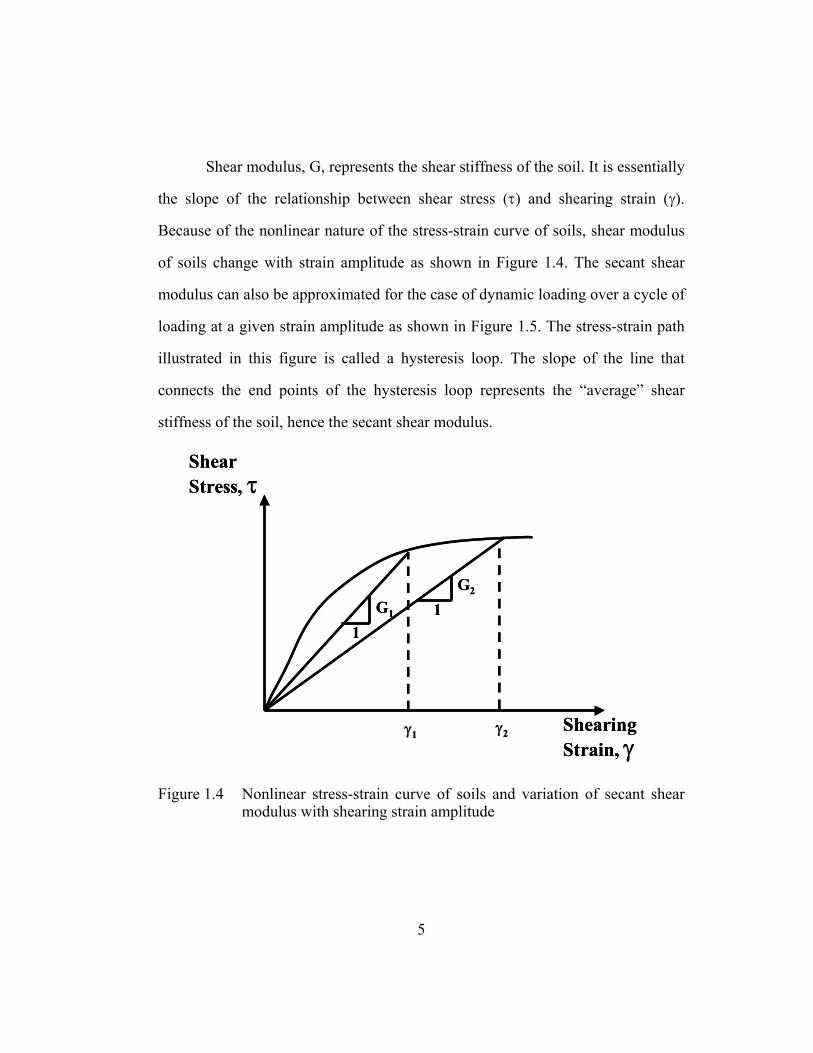
Shear modulus, G, represents the shear stiffness of the soil. It is essentially
the slope of the relationship between shear stress (τ) and shearing strain (γ).
Because of the nonlinear nature of the stress-strain curve of soils, shear modulus
of soils change with strain amplitude as shown in Figure 1.4. The secant shear
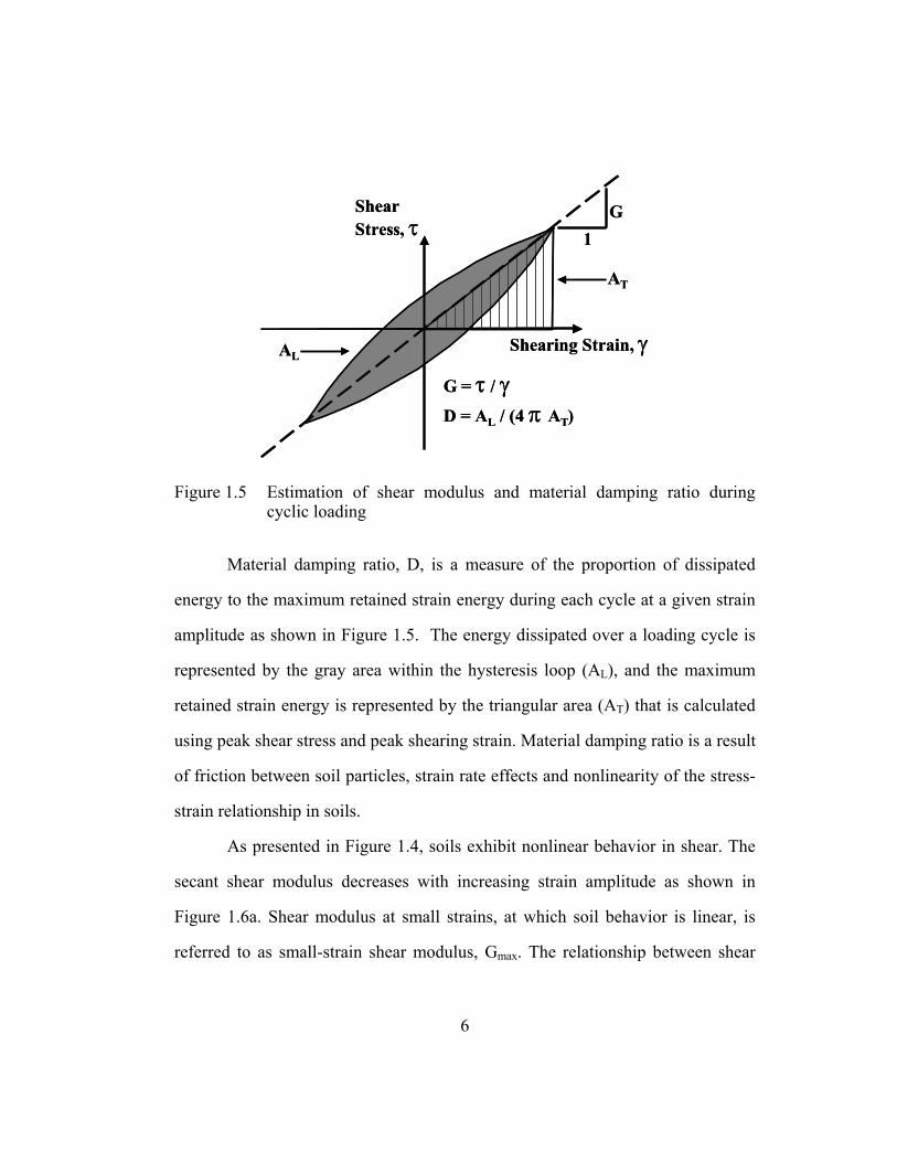
modulus can also be approximated for the case of dynamic loading over a cycle of
loading at a given strain amplitude as shown in Figure 1.5. The stress-strain path
illustrated in this figure is called a hysteresis loop. The slope of the line that
connects the end points of the hysteresis loop represents the “average” shear
stiffness of the soil, hence the secant shear modulus.
1G1
γ1 γ2
1G2
ShearStress, τ
ShearingStrain, γ
1G1
γ1 γ2
1G2
ShearStress, τ
ShearingStrain, γ
Figure 1.4 Nonlinear stress-strain curve of soils and variation of secant shear modulus with shearing strain amplitude
6
1GShear
Stress, τ
Shearing Strain, γ
G = τ / γD = AL / (4 π AT)
AL
AT
1GShear
Stress, τ
Shearing Strain, γ
G = τ / γD = AL / (4 π AT)
AL
AT
Figure 1.5 Estimation of shear modulus and material damping ratio during cyclic loading
Material damping ratio, D, is a measure of the proportion of dissipated
energy to the maximum retained strain energy during each cycle at a given strain
amplitude as shown in Figure 1.5. The energy dissipated over a loading cycle is
represented by the gray area within the hysteresis loop (AL), and the maximum
retained strain energy is represented by the triangular area (AT) that is calculated
using peak shear stress and peak shearing strain. Material damping ratio is a result
of friction between soil particles, strain rate effects and nonlinearity of the stress-
strain relationship in soils.
As presented in Figure 1.4, soils exhibit nonlinear behavior in shear. The
secant shear modulus decreases with increasing strain amplitude as shown in
Figure 1.6a. Shear modulus at small strains, at which soil behavior is linear, is
referred to as small-strain shear modulus, Gmax. The relationship between shear

7
modulus and strain amplitude is typically characterized by a normalized modulus
reduction curve as shown in Figure 1.6b.
Gmax
120
80
40
00.001 0.01 0.1 1
Shearing Strain, γ , %
G,MPa
1.0
0.5
00.001 0.01 0.1 1
Shearing Strain, γ , %
GGmax
(a) (b)
Gmax
120
80
40
00.001 0.01 0.1 1
Shearing Strain, γ , %
G,MPa
1.0
0.5
00.001 0.01 0.1 1
Shearing Strain, γ , %
GGmaxGmax
120
80
40
00.001 0.01 0.1 1
Shearing Strain, γ , %
G,MPa Gmax
120
80
40
00.001 0.01 0.1 1
Shearing Strain, γ , %
G,MPa
1.0
0.5
00.001 0.01 0.1 1
Shearing Strain, γ , %
GGmax
1.0
0.5
00.001 0.01 0.1 1
Shearing Strain, γ , %
GGmax
(a) (b)
Figure 1.6 (a) Nonlinear shear modulus and (b) normalized modulus reduction curves
The nonlinearity in the stress-strain relationship results in an increase in
energy dissipation and, therefore, an increase in material damping ratio with
increasing strain amplitude as presented in Figure 1.7. Material damping ratio at
small strains (in the linear range) is referred to as small-strain material damping
ratio, Dmin, herein.
DminD,%
16
8
00.001 0.01 0.1 1
Shearing Strain, γ , %
DminD,%
16
8
00.001 0.01 0.1 1
Shearing Strain, γ , %
Figure 1.7 Nonlinear material damping ratio curve

8
1.3 GROUND RESPONSE ANALYSIS
In analyzing ground motions due to small vibrations, soil behavior is
assumed to be linear. Each soil layer is assigned a shear modulus and a material
damping ratio. Since a horizontally layered system is being modeled, the task of
ground response analysis is reduced to a simple 1-D wave propagation problem
that has a closed-form solution (Kramer, 1996).
On the other hand, dynamic soil properties can be extremely nonlinear
when ground motions are caused by large vibrations (such as design level
earthquakes). As a result, the change in shear modulus and material damping ratio
with shearing strain amplitude must be accounted for in ground response analysis.
The linear solution, which is applicable for small vibration levels, can be modified
to overcome this problem.
One approach to handling nonlinear soil behavior due to shaking during a
design level event is to perform linear analyses with dynamic soil properties that
are iterated in a manner consistent with an “effective” shearing strain induced in
the soil layer (Schnabel et al., 1972; and EduPro, 1998). This iterative approach is
called equivalent linear analysis.
The effective shearing strain is defined as a certain portion of the
maximum strain amplitude throughout the time history. The ratio of effective
shearing strain to maximum strain amplitude is typically related to the magnitude
of the earthquake event or the characteristics of the acceleration-time record
employed in the analysis. When a design level earthquake is analyzed, the ratio of
effective to maximum shearing strain is typically about 0.6.
9
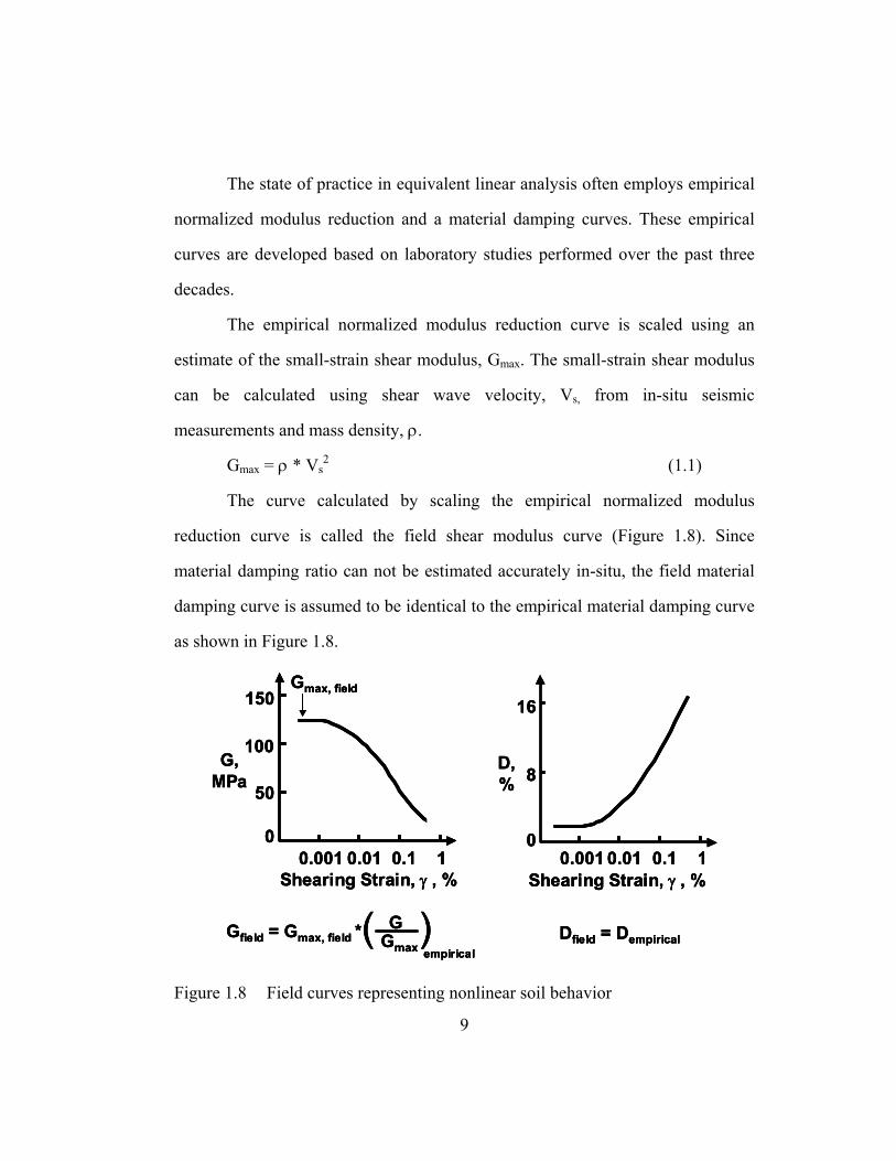
The state of practice in equivalent linear analysis often employs empirical
normalized modulus reduction and a material damping curves. These empirical
curves are developed based on laboratory studies performed over the past three
decades.
The empirical normalized modulus reduction curve is scaled using an
estimate of the small-strain shear modulus, Gmax. The small-strain shear modulus
can be calculated using shear wave velocity, Vs, from in-situ seismic
measurements and mass density, ρ.
Gmax = ρ * Vs2 (1.1)
The curve calculated by scaling the empirical normalized modulus
reduction curve is called the field shear modulus curve (Figure 1.8). Since
material damping ratio can not be estimated accurately in-situ, the field material
damping curve is assumed to be identical to the empirical material damping curve
as shown in Figure 1.8.
Dfield = Dempirical
D,%
16
8
00.001 0.01 0.1 1
Shearing Strain, γ , %
150
100
50
00.001 0.01 0.1 1
Shearing Strain, γ , %
G,MPa
Gfield = Gmax, field *empirical
( )GGmax
Gmax, field
Dfield = Dempirical
D,%
16
8
00.001 0.01 0.1 1
Shearing Strain, γ , %
Dfield = Dempirical
D,%
16
8
00.001 0.01 0.1 1
Shearing Strain, γ , %
150
100
50
00.001 0.01 0.1 1
Shearing Strain, γ , %
G,MPa
Gfield = Gmax, field *empirical
( )GGmax
Gmax, field150
100
50
00.001 0.01 0.1 1
Shearing Strain, γ , %
G,MPa
Gfield = Gmax, field *empirical
( )GGmax
Gmax, field
Figure 1.8 Field curves representing nonlinear soil behavior

10
1.4 OBJECTIVES OF RESEARCH
As part of various research projects [including the SRS (Savannah River
Site) Project AA891070, EPRI (Electric Power Research Institute) Project 3302,
and ROSRINE (Resolution of Site Response Issues from the Northridge
Earthquake) Project] numerous sites were drilled and sampled. Intact soil samples
over a depth range of several hundred meters were recovered from 20 of these
sites. These soil samples were tested in the soil dynamics laboratory at The
University of Texas at Austin (UTA) to characterize the materials.
The presence of a database accumulated from testing these intact
specimens motivated a re-evaluation of empirical curves often employed in
seismic site response analyses. The weaknesses of empirical curves reported in
the literature were recognized and the necessity of developing an improved set of
empirical curves was acknowledged.
This study focuses on generating an improved set of empirical curves that
can be represented in the form of a set of simple equations. The data collected
over the past decade at The University of Texas at Austin are statistically
analyzed using the First-order, Second-moment Bayesian Method (FSBM). The
effects of various parameters (such as confining pressure and soil plasticity) on
dynamic soil properties are evaluated and quantified within this framework.
One of the most important aspects of this study is estimating not only the
mean values of the empirical curves but also the uncertainty associated with these
values. The handling of uncertainty in the empirical estimates of dynamic soil
11
properties is expected to result in a refinement of probabilistic seismic hazard
analysis.
1.5 ORGANIZATION OF DISSERTATION
A general overview of the dynamic laboratory test equipment used to
evaluate the nonlinear soil properties is presented in Chapter Two along with a
brief review of the theory upon which the laboratory testing is founded.
Information regarding the soil samples analyzed in this work is
summarized in Chapter Three. All testing was conducted at The University of
Texas at Austin over the past decade.
The sensitivity of dynamic soil properties to soil type and loading
conditions are described in Chapter Four. The general trends (in terms of how
these parameters affect nonlinear soil behavior) observed during the course of this
work and those reported in the literature are discussed.
The empirical relationships reported in the literature are summarized in
Chapter Five. The empirical normalized modulus reduction and material damping
curves proposed in the literature are evaluated in terms of capturing the general
trends discussed in Chapter Four.
A four-parameter soil model that describes the change in normalized shear
modulus and material damping ratio with shearing strain is presented in Chapter
Six along with a parametric study of the model. Two of these parameters,
reference strain and curvature coefficient, are utilized in describing the
normalized modulus reduction curve. Masing behavior is used as a criterion in
evaluating material damping. A scaling coefficient and small-strain material

12
damping ratio are utilized in describing the material damping curve relative to the
damping curve estimated from the normalized modulus reduction curve and
assuming Masing Behavior. The impact of soil type and loading conditions on the
model parameters are also described herein.
The First-order, Second-moment Bayesian method is briefly discussed in
Chapter Seven. The form of the equations that are used in relating model
parameters to soil type and loading conditions are discussed in this chapter.
Results of the statistical analysis are presented in Chapter Eight. Measured
and predicted curves are compared in order to evaluate the success of the model in
representing nonlinear soil behavior.
In Chapter Nine, the impact of soil type and loading conditions on model
parameters are quantified. Equations and graphical solutions that are utilized to
construct normalized shear modulus reduction and material damping curves for
different soil types and loading conditions are presented. These curves are
compared with other empirical curves reported in the literature.
In Chapter Ten, recommended normalized modulus reduction and material
damping curves are presented for soils with a broad range plasticity confined at
different mean effective stresses.
Uncertainty associated with the predicted normalized modulus reduction
and material damping curves is discussed in Chapter Eleven. Recommendations
for future work related with handling uncertainty in nonlinear soil behavior are
presented for probabilistic seismic hazard analysis.
A summary of the study and conclusions are presented in Chapter Twelve.
13
CHAPTER 2
LABORATORY TESTING EQUIPMENT
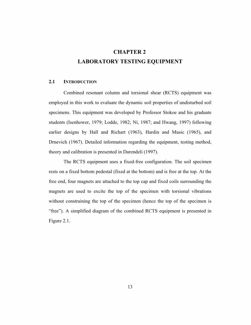
2.1 INTRODUCTION
Combined resonant column and torsional shear (RCTS) equipment was
employed in this work to evaluate the dynamic soil properties of undisturbed soil
specimens. This equipment was developed by Professor Stokoe and his graduate
students (Isenhower, 1979; Lodde, 1982; Ni, 1987; and Hwang, 1997) following
earlier designs by Hall and Richart (1963), Hardin and Music (1965), and
Drnevich (1967). Detailed information regarding the equipment, testing method,
theory and calibration is presented in Darendeli (1997).
The RCTS equipment uses a fixed-free configuration. The soil specimen
rests on a fixed bottom pedestal (fixed at the bottom) and is free at the top. At the
free end, four magnets are attached to the top cap and fixed coils surrounding the
magnets are used to excite the top of the specimen with torsional vibrations
without constraining the top of the specimen (hence the top of the specimen is
“free”). A simplified diagram of the combined RCTS equipment is presented in
Figure 2.1.

14
Proximitor ProbesAccelerometer
SupportPlate
Fluid Bath
SecuringPlate
Magnet
InnerCylinder
Specimen
PorousStone O-ring
RubberMembrane
Top Cap
Resonant or Slow CyclicTorsional Excitation
Counter Weight
DriveCoil
Base Plate
Proximitor TargetProximitor ProbesAccelerometer
SupportPlate
Fluid Bath
SecuringPlate
Magnet
InnerCylinder
Specimen
PorousStone O-ring
RubberMembrane
Top Cap
Resonant or Slow CyclicTorsional Excitation
Counter Weight
DriveCoil
Base Plate
Proximitor Target
Figure 2.1 Simplified diagram of the RCTS device (from Stokoe et al., 1999)
2.2 COMBINED RESONANT COLUMN AND TORSIONAL SHEAR EQUIPMENT
Combined RCTS equipment is capable of testing a soil specimen in two
different modes. These modes are: 1. low frequency cyclic testing, and 2. higher
frequency dynamic testing during resonance. Thus, the same specimen can be
tested using both modes and variability due to testing different specimens or
testing the same specimen after it has been subjected to a different stress history is
eliminated. The data collected from the two independent modes of testing can
effectively be compared in order to gain more insight regarding material behavior.
One of the testing modes is called the torsional resonant column (RC) test,
which is based on the theory of torsional wave propagation in a fixed-free
cylinder with a mass attached at the free end. In this mode, well-defined boundary
15
conditions and specimen geometry are utilized in evaluating the shear modulus
and material damping ratio in shear from measurements at first-mode resonance.
The second testing mode is called the cyclic torsional shear (TS) test,
which involves monitoring the applied torque and displacement at the top of the
specimen. The torque is converted into shear stress and the displacement is
converted into shearing strain. Thus, hysteresis loops, which are utilized in
evaluation of shear modulus and material damping ratio, are generated.
These tests are typically carried out while the specimen is confined
isotropically. The confining chamber is designed to handle pressures up to 40
atmospheres (4.1 MPa). A cross-sectional view of the confining system is
presented in Figure 2.2.
AirPressure
σ
Membrane
FixingRod
Top Plate
HollowCylinder
SiliconFluid Bath
σ
σ
O-Ring
Soil
ThinMetal Tube
Drainage
Figure 2.2 Simplified cross-sectional view of the confining system (from Hwang, 1997)

16
The soil specimen is tested using both the cyclic torsional shear and
resonance modes simply by changing: 1) the amplitude and frequency of the
current in the drive coils, and 2) the motion monitoring devices (shown in Figure
2.3) used to record the specimen response. These changes are performed outside
the confining chamber; hence, they can be done without changing the state of
stress on the specimen.
2.3 TORSIONAL RESONANT COLUMN TEST
In torsional RC testing, a forcing function with fixed amplitude and
varying frequency is applied at the top of a cylindrical soil specimen. The output
from the accelerometer on the drive plate (shown in Figure 2.3) is recorded versus
the vibration frequency during a frequency sweep. The graph of accelerometer
output versus vibration frequency is called the frequency response curve. A
typical response curve is shown in Figure 2.4. The frequency at which the
accelerometer output reaches a maximum during first-mode torsional resonance is
denoted as the resonant frequency, fr, and it is used in calculating the shear wave
velocity of the specimen. The value of accelerometer output, Ar, at this frequency
is then used in calculating the peak shearing strain amplitude during the test.
The frequency response curve is also utilized in evaluating the material
damping ratio at small shearing strains, γ, (γ < 0.005 %). The half-power points
are identified as the two points on the frequency response curve with an amplitude
of 1/√2 times the peak value. The frequencies associated with the half-power
points, f1 and f2, are used in evaluating the material damping ratio as presented in
Figure 2.5.
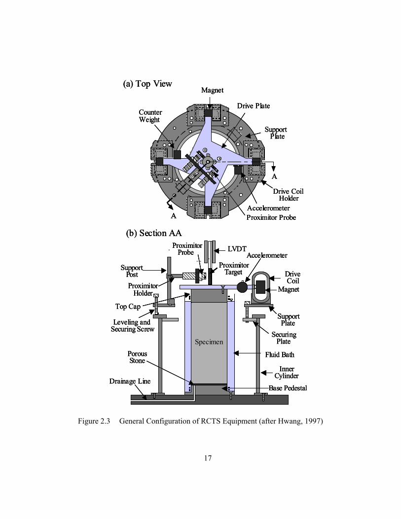
17
SupportPlate
CounterWeight
Drive Plate
Accelerometer
Magnet
Drive CoilHolder
A
A Proximitor Probe
(a) Top View
Leveling andS
LVDT
ProximitorTarget
Accelerometer
ecuring Screw
SupportPlate
Fluid Bath
SecuringPlate
Magnet
DriveCoil
InnerCylinder
Base Pedestal
ProximitorProbe
SupportPostProximitor
Holder
PorousStone
(b) Section AA
Drainage Line
Top Cap
Specimen
SupportPlate
CounterWeight
Drive Plate
Accelerometer
Magnet
Drive CoilHolder
A
A Proximitor Probe
(a) Top View
SupportPlate
CounterWeight
Drive Plate
Accelerometer
Magnet
Drive CoilHolder
A
A Proximitor Probe
(a) Top View
Leveling andS
LVDT
ProximitorTarget
Accelerometer
ecuring Screw
SupportPlate
Fluid Bath
SecuringPlate
Magnet
DriveCoil
InnerCylinder
Base Pedestal
ProximitorProbe
SupportPostProximitor
Holder
PorousStone
(b) Section AA
Drainage Line
Top Cap
Specimen
Leveling andS
LVDT
ProximitorTarget
Accelerometer
ecuring Screw
SupportPlate
Fluid Bath
SecuringPlate
Magnet
DriveCoil
InnerCylinder
Base Pedestal
ProximitorProbe
SupportPostProximitor
Holder
PorousStone
(b) Section AA
Drainage Line
Top Cap
Specimen
Figure 2.3 General Configuration of RCTS Equipment (after Hwang, 1997)

18
I/Io=(ωrL/Vs) tan(ωrL/Vs)
G = ρVs2
→γAr
f = / 2πrr ω
605550454035
120
80
40
0
Ar
Acc
eler
omet
er O
utpu
t, m
V Resonance
Frequency, f, Hz
Figure 2.4 Frequency response curve measured in the RC test (from Stokoe et al., 1999)
Figure 2.5 Material damping measurement in the RC test using the half-power bandwidth (from Stokoe et al., 1999)

19
Once the resonant frequency is identified, a second measurement of
material damping ratio can be performed using the free-vibration decay curve.
This method involves vibrating the specimen in steady-state, first-mode torsional
resonance and recording the decay of free vibrations after shutting off the driving
force. Figure 2.6 shows an example decay curve. Sh
earin
g St
rain
Am
plitu
de, γ
x 1
0-3, %
0.40.30.20.10.0Time, seconds
0
1
2
3
-1
-2
-3
(a)1
510
15
Steady State Free Vibration Decay
CycleNumber
Nor
mal
ized
Pea
k-to
-Pea
k A
mpl
itude
s
20151050Number of Cycles
Remolded Sandeo = 0.71δ = 0.0734D = 1.17 %
(b)
1.0
0.7
0.5
0.3
Figure 2.6 Material damping measurement in the RC test using the free-vibration decay curve (from Stokoe et al., 1999)

20
The logarithmic decrement, δ, is defined from the free-vibration decay
curve as:
=
+1
1ln1
nzz
nδ (2.1)
where n equals number of cycles between two peak points in the time record, and
z1 and zn+1 are the amplitudes of cycle 1 and cycle n+1, respectively (Richart, Hall
and Woods, 1970). Material damping ratio can then be calculated using Equation
2.2.
22
2
4 δδ
+Π=D (2.2)
The half-power bandwidth method is based on the theory of elasticity and
it is accurate during testing at small strains as noted above (γ < 0.005 %). Material
damping estimates based on this method are quite reproducible at small strains
since points around the peak output on the frequency response curve are utilized
in the calculations. On the other hand, background noise can have a more adverse
effect on the free-vibration decay curve.
At large strains, nonlinear behavior of soil results in the linear assumption,
on which the half-power bandwidth method is based, to become invalid. In this
case, the free-vibration decay curve is applied along with an adjustment of the
strain amplitude, which is constantly changing as the vibrations decay. In the free-
vibration decay method, material damping ratio is calculated using the first three
cycles of vibration in this study. As a result, the average amplitude of the first
three cycles of vibration is assumed to represent the shearing strain at which the
measurement is made (rather than the steady-state amplitude).

21
2.4 CYCLIC TORSIONAL SHEAR TEST
In cyclic TS testing, a slow torsional loading is applied at the top of the
specimen. The loading frequency used in TS testing is much lower than resonance
testing (at least 10 times less than the resonant frequency). The current in the
calibrated drive coils is monitored, and the torque applied to the specimen is
calculated. The displacement at the top of the specimen is also monitored using
proximitors. Based on the torque and displacement at the top of the specimen,
hysteresis loops are generated.
The secant shear modulus for each cycle of loading is evaluated by
calculating the slope of the line that connects the end points of the hysteresis loop
as illustrated in Figure 2.7.
1GShear
Stress, τ
Shearing Strain, γ
G = τ / γD = AL / (4 π AT)
AL
AT
1GShear
Stress, τ
Shearing Strain, γ
G = τ / γD = AL / (4 π AT)
G = τ / γD = AL / (4 π AT)
AL
AT
Figure 2.7 Calculation of shear modulus and material damping ratio in the TS test

22
Material damping ratio is evaluated by calculating the ratio of the area
within the hysteresis loop (AL) and the maximum potential energy stored in each
cycle of motion as represented by the triangular area (AT). The area AT is
calculated using the end point of the hysteresis loop as shown in Figure 2.7.
T
L
AADΠ
=4
(2.3)
2.5 SUMMARY
Information regarding the RCTS equipment is summarized in this chapter.
This equipment has been employed in evaluating nonlinear dynamic soil
properties of undisturbed soil specimens for more than two decades at The
University of Texas at Austin. Detailed information regarding the equipment,
testing method, theory and calibration is presented in Ni (1987), Hwang (1997)
and Darendeli (1997).

23
CHAPTER 3
PHYSICAL PROPERTIES OF TEST SPECIMENS
3.1 INTRODUCTION
Over the past decade, a total of 110 undisturbed soil samples, which were
taken from 20 geotechnical sites, were tested in the soil dynamics laboratory
using the combined RCTS equipment. In this study, dynamic properties of these
soils in the nonlinear range are analyzed. Information regarding the soil samples
and the confining pressures at which these samples were tested are tabulated in
this chapter. Also, the geotechnical reports that contain the original data are cited
herein.
The chapter has been divided into the following sections. Sections 3.2
through 3.5 describe samples taken from Northern California, Southern
California, South Carolina and Lotung, Taiwan, respectively. In each section,
information regarding specimens from each geotechnical site in a given
geographic region is presented in a separate table. As an example, Table 3.1
shows physical properties of soils recovered from Oakland Outer Harbor. The
publication that contains the original data is cited in the title of the table. The table
provides the following information on each specimen: 1) Specimen identification
(ID), 2) Depth of the soil sample, 3) Soil type determined according to the Unified
Soil Classification System (USCS) based on gradation and plasticity tests
performed at The University of Texas at Austin, 4) Percentage of fine material
(passing #200 sieve) by weight (listed as Fines Content), 5) Liquid limit (LL), 6)
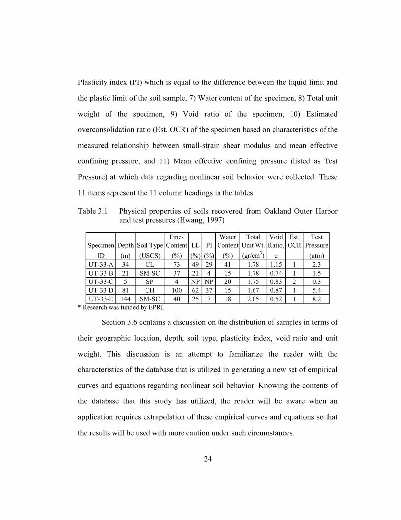
24
Plasticity index (PI) which is equal to the difference between the liquid limit and
the plastic limit of the soil sample, 7) Water content of the specimen, 8) Total unit
weight of the specimen, 9) Void ratio of the specimen, 10) Estimated
overconsolidation ratio (Est. OCR) of the specimen based on characteristics of the
measured relationship between small-strain shear modulus and mean effective
confining pressure, and 11) Mean effective confining pressure (listed as Test
Pressure) at which data regarding nonlinear soil behavior were collected. These
11 items represent the 11 column headings in the tables.
Table 3.1 Physical properties of soils recovered from Oakland Outer Harbor and test pressures (Hwang, 1997)
Fines Water Total Void Est. TestSpecimen Depth Soil Type Content LL PI Content Unit Wt. Ratio, OCR Pressure
ID (m) (USCS) (%) (%) (%) (%) (gr/cm3) e (atm)UT-33-A 34 CL 73 49 29 41 1.78 1.15 1 2.3UT-33-B 21 SM-SC 37 21 4 15 1.78 0.74 1 1.5UT-33-C 5 SP 4 NP NP 20 1.75 0.83 2 0.3UT-33-D 81 CH 100 62 37 15 1.67 0.87 1 5.4UT-33-E 144 SM-SC 40 25 7 18 2.05 0.52 1 8.2
* Research was funded by EPRI.
Section 3.6 contains a discussion on the distribution of samples in terms of
their geographic location, depth, soil type, plasticity index, void ratio and unit
weight. This discussion is an attempt to familiarize the reader with the
characteristics of the database that is utilized in generating a new set of empirical
curves and equations regarding nonlinear soil behavior. Knowing the contents of
the database that this study has utilized, the reader will be aware when an
application requires extrapolation of these empirical curves and equations so that
the results will be used with more caution under such circumstances.

25
3.2 UNDISTURBED SOIL SPECIMENS FROM NORTHERN CALIFORNIA
A total of 37 undisturbed soil samples from 7 sites in Northern California
tested as part of a number of research projects are included in this study. These
projects were funded by the Kajima Corporation, Geovision, Agbabian
Associates, EPRI (Electric Power Research Institute), Fugro, Inc., and Earth
Mechanics, Inc.
The geotechnical sites in Northern California are Corralitos, Garner
Valley, Gilroy, Oakland Outer Harbor, San Francisco Airport, San Francisco-
Oakland Bay Bridge and Treasure Island. A map of Northern California is
presented in Figure 3.1 showing the locations of these sites. Information regarding
the soil samples and the confining pressures at which nonlinear properties were
measured are tabulated in Tables 3.1 through 3.7. The references that contain the
original data are also cited in the titles of the tables.
Table 3.2 Physical properties of soils recovered from Treasure Island and test pressures (Hwang and Stokoe, 1993b; and Hwang, 1997)
Fines Water Total Void Est. TestSpecimen Depth Soil Type Content LL PI Content Unit Wt. Ratio, OCR Pressure
ID (m) (USCS) (%) (%) (%) (%) (gr/cm3) e (atm)UT-28-A 18 CH 50 51 26 50 1.73 1.34 1 1.2UT-28-B 52 CL 79 34 19 21 2.05 0.58 1 3.8UT-28-C 71 CL 67 48 30 33 1.84 0.95 1 5.1UT-28-D 40 CL 63 37 23 37 1.83 1.02 1 2.9UT-28-E 9.1 SP-SM 79 NP NP 21 1.92 0.67 1 0.7UT-28-F 27 CL 58 42 19 42 1.81 1.10 1 1.9UT-28-G 5.3 SM 80 NP NP 20 1.92 0.69 1 0.4UT-28-H 34 SP-SM 78 NP NP 22 1.83 0.76 1 2.2
* Research was funded by EPRI.
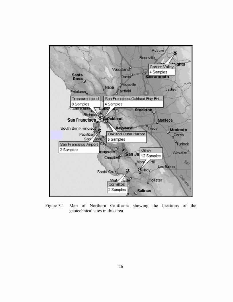
26
Figure 3.1 Map of Northern California showing the locations of the geotechnical sites in this area

27
Table 3.3 Physical properties of soils recovered from San Francisco Airport and test pressures (Hwang, 1997)
Fines Water Total Void Est. TestSpecimen Depth Soil Type Content LL PI Content Unit Wt. Ratio, OCR Pressure
ID (m) (USCS) (%) (%) (%) (%) (gr/cm3) e (atm)UT-36-A 4.9 CL-ML 53 21 5 19 2.08 0.54 2 0.3UT-36-B 7.9 CL 54 30 13 18 2.10 0.50 2 0.5
* Research was funded by EPRI.
Table 3.4 Physical properties of soils recovered from Gilroy and test pressures (Hwang and Stokoe, 1993c; Hwang, 1997; and Stokoe et al., 2001)
Fines Water Total Void Est. TestSpecimen Depth Soil Type Content LL PI Content Unit Wt. Ratio, OCR Pressure
ID (m) (USCS) (%) (%) (%) (%) (gr/cm3) e (atm)UT-24-A 6.1 CL 86 43 23 30 1.91 0.84 1 0.8UT-24-B 3.0 CL-ML 65 29 7 26 1.88 0.81 1 0.4UT-24-C 26 MH 100 47 17 31 1.94 0.82 1 2.4UT-24-D 37 ML 62 NP NP 20 2.12 0.48 1 3.3
UT-24-E++ 128 * * * * 14 2.18 0.41 1 8.7UT-24-F 64 SW-SM 8 NP NP 15 2.08 0.46 1 4.9UT-24-G 15 SP 2 NP NP 16 1.97 0.55 1 2.0UT-24-H 106 CL 65 35 13 24 2.04 0.63 1 8.6UT-24-I 6.1 CL 86 43 23 30 1.91 0.84 1 0.8UT-24-J 26 MH 100 47 17 31 1.94 0.82 1 2.4UT-24-K 37 ML 62 NP NP 20 2.12 0.48 1 3.3
UT-24-L++ 52 SM 13 NP NP 8 2.13 0.34 1 4.8UTA-18-I 3.4 SC 17 36 20 20 2.15 0.47 1 0.4UTA-18-J 16 SC 28 49 24 15 1.95 0.56 1 1.1
* Information is not available. ** Research was funded by EPRI and Kajima Corporation, Japan through Geovision. ++ UT-24-E and UT-24-L were stopped due to membrane leakage and are not included in this study.

28
Table 3.5 Physical properties of soils recovered from Garner Valley and test pressures (Stokoe and Darendeli, 1998)
Fines Water Total Void Est. TestSpecimen Depth Soil Type Content LL PI Content Unit Wt. Ratio, OCR Pressure
ID (m) (USCS) (%) (%) (%) (%) (gr/cm3) e (atm)UT-52-A 3.5 SM 26 NP NP 19 1.90 0.69 1 0.5UT-52-B 6.5 SM 15 NP NP 17 1.79 0.76 1 0.7UT-52-C 41 SM 36 NP NP 18 1.91 0.67 1 2.7UT-52-D 27 SM 19 NP NP 14 2.09 0.47 1 1.7
* Research was funded by Agbabian Associates.
Table 3.6 Physical properties of soils recovered from San Francisco-Oakland Bay Bridge Site and test pressures (Stokoe et al., 1998d)
Fines Water Total Void Est. TestSpecimen Depth Soil Type Content LL PI Content Unit Wt. Ratio, OCR Pressure
ID (m) (USCS) (%) (%) (%) (%) (gr/cm3) e (atm)UTA-10-A 8.4 CH 93 63 36 50 1.71 1.38 1 0.5, 2.2UTA-10-B 11 CH 97 75 43 58 1.63 1.61 1 0.5, 2.2UTA-10-C 24 CH 96 89 53 57 1.70 1.50 8 1.1, 4.4UTA-10-D 71 CL 91 46 19 30 1.92 0.83 1 4.1, 16.3
* Research was funded by Fugro, Inc. and Earth Mechanics, Inc.
Table 3.7 Physical properties of soils recovered from Corralitos and test pressures (Stokoe et al., 2001)
Fines Water Total Void Est. TestSpecimen Depth Soil Type Content LL PI Content Unit Wt. Ratio, OCR Pressure
ID (m) (USCS) (%) (%) (%) (%) (gr/cm3) e (atm)UTA-18-F 10 SW-SC 7 31 10 14 2.16 0.44 1 1.4
UTA-18-G** 3.3 SC 31 44 19 19 2.01 0.62 1 0.5UTA-18-K 46 ML 52 23 4 8 2.39 0.24 2 4.1
* Research was funded by Kajima Corporation, Japan through Geovision. ** UTA-18-G was reconstituted and is not included in this study.

29
Specimen UTA-18-G sampled from Corralitos was reconstituted.
Specimens UT-24-E and UT-24-L from Gilroy had to be stopped due to
membrane leakage before the TS data could be collected. As a result, these
samples are not included in this study, but are included in the tables for
completeness.
3.3 UNDISTURBED SOIL SPECIMENS FROM SOUTHERN CALIFORNIA
A total of 47 undisturbed soil samples from 10 sites in Southern California
tested as part of a number of research projects are included in this study. These
projects were funded by the ROSRINE (Resolution of Site Response Issues from
the Northridge Earthquake) Project, Kajima Corporation, Geovision and
Agbabian Associates.
The geotechnical sites in Southern California are Arleta, Borrego, Imperial
Valley College, Kagel, La Cienega, Newhall, North Palm Springs, Potrero
Canyon, Rinaldi Receiving Station and Sepulveda V.A. Hospital. A map of
Southern California is presented in Figure 3.2 showing the locations of the three
sites outside the Los Angeles area (Borrego, Imperial Valley College and North
Palm Springs). The remaining seven sites are presented on a map of Los Angeles
area in Figure 3.3.
Information regarding the soil samples and the confining pressures (at
which these samples were tested) are tabulated in Tables 3.8 through 3.17. The
references that contain the original data are also cited in the titles of the tables.

30
Figure 3.2 Map of Southern California showing the locations of the three geotechnical sites outside the Los Angeles area
Specimen UT-40-G from Borrego was stopped due to membrane leakage
before the TS data could be collected. Specimens UTA-9-I from Rinaldi
Receiving Station, and UTA-18-B and UTA-18-E from North Palm Springs were
reconstituted. As a result, these samples are not included in this study, but are
included in the tables for completeness.
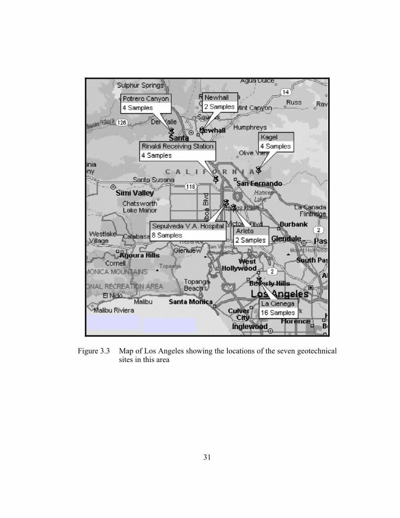
31
Figure 3.3 Map of Los Angeles showing the locations of the seven geotechnical sites in this area

32
Table 3.8 Physical properties of soils recovered from Borrego and test pressures (Hwang, 1997)
Fines Water Total Void Est. TestSpecimen Depth Soil Type Content LL PI Content Unit Wt. Ratio, OCR Pressure
ID (m) (USCS) (%) (%) (%) (%) (gr/cm3) e (atm)UT-40-B 3.4 SM 84 NP NP 12 1.76 0.68 1 0.4UT-40-C 20 SP-SM 89 NP NP 11 1.83 0.62 1 2.5UT-40-E 49 SP-SM 91 NP NP 14 1.76 0.72 1 6.1UT-40-F 110 SP-SM 91 NP NP 17 1.78 0.75 1 13.6
UT-40-G** 146 SP-SM 95 NP NP 11 2.04 0.44 1 18.2 * Research was funded by Agbabian Associates. ** UT-40-G was stopped due to membrane leakage and is not included in this study.
Table 3.9 Physical properties of soils recovered from Arleta and test pressures (Darendeli and Stokoe, 1997; and Darendeli, 1997)
Fines Water Total Void Est. TestSpecimen Depth Soil Type Content LL PI Content Unit Wt. Ratio, OCR Pressure
ID (m) (USCS) (%) (%) (%) (%) (gr/cm3) e (atm)UTA-1-C 31 SM 40 21 1 13 2.16 0.42 2 2.7, 10.9UTA-1-L 15 SM 28 NP NP 14 2.10 0.46 1 1.6
* Research was funded by ROSRINE Project.
Table 3.10 Physical properties of soils recovered from Kagel and test pressures (Darendeli and Stokoe, 1997; and Darendeli, 1997)
Fines Water Total Void Est. TestSpecimen Depth Soil Type Content LL PI Content Unit Wt. Ratio, OCR Pressure
ID (m) (USCS) (%) (%) (%) (%) (gr/cm3) e (atm)UTA-1-E 8.5 SW-SM 10 NP NP 3 1.87 0.48 1 1.1, 4.4UTA-1-F 31 SW-SM 12 NP NP 13 2.11 0.44 1 3.3UTA-1-G 65 SW-SM 9 NP NP 10 2.16 0.38 1 5.4UTA-1-H 92 SP-SM 10 NP NP 13 2.07 0.46 1 6.8
* Research was funded by ROSRINE Project.
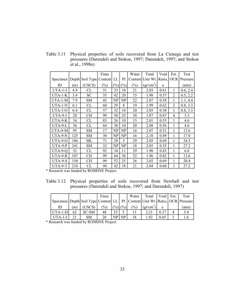
33
Table 3.11 Physical properties of soils recovered from La Cienega and test pressures (Darendeli and Stokoe, 1997; Darendeli, 1997; and Stokoe et al., 1998e)
Fines Water Total Void Est. TestSpecimen Depth Soil Type Content LL PI Content Unit Wt. Ratio, OCR Pressure
ID (m) (USCS) (%) (%) (%) (%) (gr/cm3) e (atm)UTA-1-J 4.9 CL 51 33 10 21 2.03 0.61 1 0.6, 2.4UTA-1-K 3.4 SC 35 42 20 15 1.98 0.57 2 0.5, 2.2UTA-1-M 7.9 SM 43 NP NP 22 2.07 0.58 1 1.1, 4.4UTA-1-N 6.1 CL 60 29 8 19 1.99 0.62 2 0.8, 3.3UTA-1-O 6.4 CL 57 32 10 20 2.05 0.58 1 0.8, 3.3UTA-9-J 28 CH 99 50 25 30 1.87 0.87 4 3.3UTA-9-K 34 CL 83 26 10 15 2.01 0.55 1 4.6UTA-9-L 36 CL 64 30 10 20 2.08 0.56 1 4.6UTA-9-M 95 SM 17 NP NP 16 2.07 0.51 1 13.6UTA-9-N 125 SM 30 NP NP 16 2.10 0.49 1 17.0UTA-9-O 186 ML 71 28 5 29 2.05 0.69 1 24.5UTA-9-P 241 SM 32 NP NP 18 2.05 0.55 1 27.2UTA-9-Q 52 CL 92 34 11 29 1.90 0.83 1 6.8UTA-9-R 107 CH 99 64 36 32 1.96 0.82 1 13.6UTA-9-S 150 CH 99 52 25 26 2.02 0.69 1 20.4UTA-9-T 218 CL 94 42 18 21 2.04 0.60 1 27.2
* Research was funded by ROSRINE Project.
Table 3.12 Physical properties of soils recovered from Newhall and test pressures (Darendeli and Stokoe, 1997; and Darendeli, 1997)
Fines Water Total Void Est. TestSpecimen Depth Soil Type Content LL PI Content Unit Wt. Ratio, OCR Pressure
ID (m) (USCS) (%) (%) (%) (%) (gr/cm3) e (atm)UTA-1-D 62 SC-SM 48 25 5 13 2.21 0.37 4 5.4UTA-1-I 21 SM 26 NP NP 18 1.92 0.65 1 1.6
* Research was funded by ROSRINE Project.

34
Table 3.13 Physical properties of soils recovered from Sepulveda V.A. Hospital and test pressures (Darendeli and Stokoe, 1997; and Darendeli, 1997)
Fines Water Total Void Est. TestSpecimen Depth Soil Type Content LL PI Content Unit Wt. Ratio, OCR Pressure
ID (m) (USCS) (%) (%) (%) (%) (gr/cm3) e (atm)UTA-1-A 3.4 CL 75 39 15 19 2.04 0.58 8 0.7UTA-1-B 3.1 CL 62 37 15 20 1.91 0.70 8 0.5UTA-1-P 14 ML 85 34 9 26 1.93 0.77 1 1.6UTA-1-Q 17 SM 41 NP NP 15 2.00 0.55 1 2.2UTA-1-R 37 CL 64 29 9 18 2.07 0.54 1 3.4UTA-1-S 59 CL 66 42 16 22 2.14 0.54 2 5.4UTA-1-T 2.4 CH 70 54 29 25 2.02 0.67 8 0.3, 1.4UTA-1-U 86 CL 77 35 12 17 2.11 0.50 1 6.8
* Research was funded by ROSRINE Project.
Table 3.14 Physical properties of soils recovered from Potrero Canyon and test pressures (Stokoe et al., 1998e)
Fines Water Total Void Est. TestSpecimen Depth Soil Type Content LL PI Content Unit Wt. Ratio, OCR Pressure
ID (m) (USCS) (%) (%) (%) (%) (gr/cm3) e (atm)UTA-9-C 8.5 SC-SM 20 19 5 11 2.15 0.39 1 1.1UTA-9-D 16 CL 73 26 9 16 2.13 0.47 1 1.9UTA-9-E 31 CL 83 32 12 10 2.32 0.28 1 4.4UTA-9-G 2.4 SM 41 20 2 21 1.88 0.74 1 0.4
* Research was funded by ROSRINE Project.
Table 3.15 Physical properties of soils recovered from Rinaldi Receiving Station and test pressures (Stokoe et al., 1998e).
Fines Water Total Void Est. TestSpecimen Depth Soil Type Content LL PI Content Unit Wt. Ratio, OCR Pressure
ID (m) (USCS) (%) (%) (%) (%) (gr/cm3) e (atm)UTA-9-A 11 SM 22 23 1 15 2.04 0.51 1 1.4UTA-9-B 21 CL-ML 53 23 5 24 1.99 0.69 1 2.4UTA-9-F 2.4 CL-ML 51 22 4 22 2.03 0.62 1 0.4UTA-9-H 15 SM 41 NP NP 16 2.03 0.55 1 1.6
UTA-9-I** 7.6 SW-SM 9 NP NP 12 2.10 0.44 1 1.1 * Research was funded by ROSRINE Project. ** UTA-9-I was reconstituted and is not included in this study.
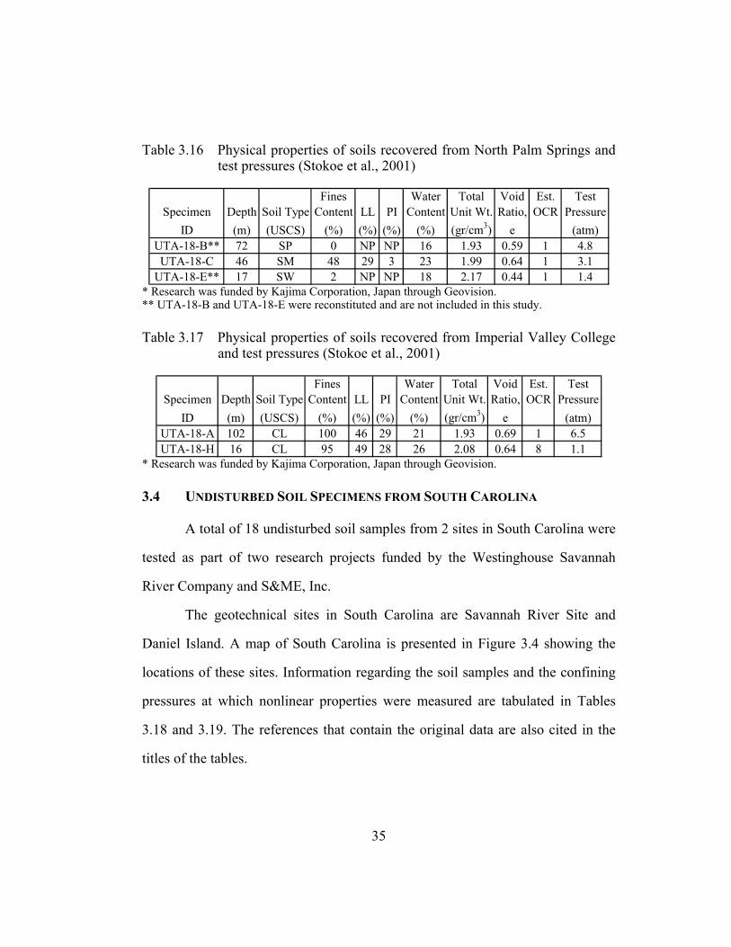
35
Table 3.16 Physical properties of soils recovered from North Palm Springs and test pressures (Stokoe et al., 2001)
Fines Water Total Void Est. TestSpecimen Depth Soil Type Content LL PI Content Unit Wt. Ratio, OCR Pressure
ID (m) (USCS) (%) (%) (%) (%) (gr/cm3) e (atm)UTA-18-B** 72 SP 0 NP NP 16 1.93 0.59 1 4.8UTA-18-C 46 SM 48 29 3 23 1.99 0.64 1 3.1
UTA-18-E** 17 SW 2 NP NP 18 2.17 0.44 1 1.4 * Research was funded by Kajima Corporation, Japan through Geovision. ** UTA-18-B and UTA-18-E were reconstituted and are not included in this study.
Table 3.17 Physical properties of soils recovered from Imperial Valley College and test pressures (Stokoe et al., 2001)
Fines Water Total Void Est. TestSpecimen Depth Soil Type Content LL PI Content Unit Wt. Ratio, OCR Pressure
ID (m) (USCS) (%) (%) (%) (%) (gr/cm3) e (atm)UTA-18-A 102 CL 100 46 29 21 1.93 0.69 1 6.5UTA-18-H 16 CL 95 49 28 26 2.08 0.64 8 1.1
* Research was funded by Kajima Corporation, Japan through Geovision.
3.4 UNDISTURBED SOIL SPECIMENS FROM SOUTH CAROLINA
A total of 18 undisturbed soil samples from 2 sites in South Carolina were
tested as part of two research projects funded by the Westinghouse Savannah
River Company and S&ME, Inc.
The geotechnical sites in South Carolina are Savannah River Site and
Daniel Island. A map of South Carolina is presented in Figure 3.4 showing the
locations of these sites. Information regarding the soil samples and the confining
pressures at which nonlinear properties were measured are tabulated in Tables
3.18 and 3.19. The references that contain the original data are also cited in the
titles of the tables.

36
Figure 3.4 Map of South Carolina showing the locations of the geotechnical sites in this area
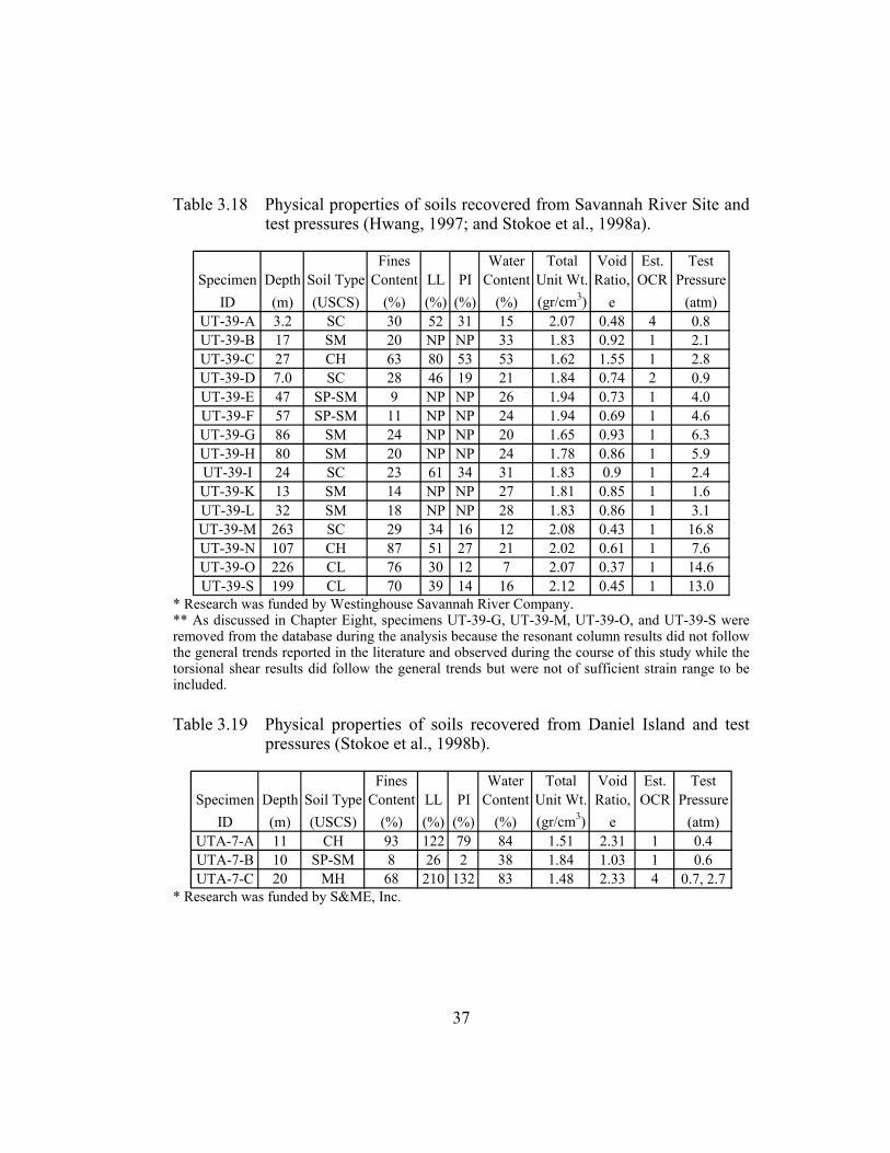
37
Table 3.18 Physical properties of soils recovered from Savannah River Site and test pressures (Hwang, 1997; and Stokoe et al., 1998a).
Fines Water Total Void Est. TestSpecimen Depth Soil Type Content LL PI Content Unit Wt. Ratio, OCR Pressure
ID (m) (USCS) (%) (%) (%) (%) (gr/cm3) e (atm)UT-39-A 3.2 SC 30 52 31 15 2.07 0.48 4 0.8UT-39-B 17 SM 20 NP NP 33 1.83 0.92 1 2.1UT-39-C 27 CH 63 80 53 53 1.62 1.55 1 2.8UT-39-D 7.0 SC 28 46 19 21 1.84 0.74 2 0.9UT-39-E 47 SP-SM 9 NP NP 26 1.94 0.73 1 4.0UT-39-F 57 SP-SM 11 NP NP 24 1.94 0.69 1 4.6UT-39-G 86 SM 24 NP NP 20 1.65 0.93 1 6.3UT-39-H 80 SM 20 NP NP 24 1.78 0.86 1 5.9UT-39-I 24 SC 23 61 34 31 1.83 0.9 1 2.4UT-39-K 13 SM 14 NP NP 27 1.81 0.85 1 1.6UT-39-L 32 SM 18 NP NP 28 1.83 0.86 1 3.1UT-39-M 263 SC 29 34 16 12 2.08 0.43 1 16.8UT-39-N 107 CH 87 51 27 21 2.02 0.61 1 7.6UT-39-O 226 CL 76 30 12 7 2.07 0.37 1 14.6UT-39-S 199 CL 70 39 14 16 2.12 0.45 1 13.0
* Research was funded by Westinghouse Savannah River Company. ** As discussed in Chapter Eight, specimens UT-39-G, UT-39-M, UT-39-O, and UT-39-S were removed from the database during the analysis because the resonant column results did not follow the general trends reported in the literature and observed during the course of this study while the torsional shear results did follow the general trends but were not of sufficient strain range to be included.
Table 3.19 Physical properties of soils recovered from Daniel Island and test pressures (Stokoe et al., 1998b).
Fines Water Total Void Est. TestSpecimen Depth Soil Type Content LL PI Content Unit Wt. Ratio, OCR Pressure
ID (m) (USCS) (%) (%) (%) (%) (gr/cm3) e (atm)UTA-7-A 11 CH 93 122 79 84 1.51 2.31 1 0.4UTA-7-B 10 SP-SM 8 26 2 38 1.84 1.03 1 0.6UTA-7-C 20 MH 68 210 132 83 1.48 2.33 4 0.7, 2.7
* Research was funded by S&ME, Inc.

38
3.5 UNDISTURBED SOIL SPECIMENS FROM LOTUNG, TAIWAN
Eight samples from Lotung site in Taiwan were tested as part of a research
project funded by EPRI. Detailed information about this work can be found in
Hwang and Stokoe (1993a), and Hwang (1997).
A map of Taiwan is presented in Figure 3.5 showing the location of
Lotung. Information regarding the soil samples and the confining pressures at
which these samples were tested are tabulated in Table 3.20.
Lotung8 SamplesLotung8 Samples
Figure 3.5 Map of Taiwan showing the location of Lotung site
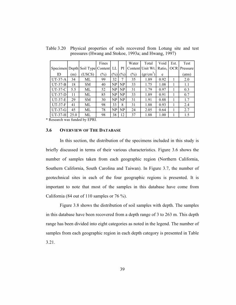
39
Table 3.20 Physical properties of soils recovered from Lotung site and test pressures (Hwang and Stokoe, 1993a; and Hwang, 1997)
Fines Water Total Void Est. TestSpecimen Depth Soil Type Content LL PI Content Unit Wt. Ratio, OCR Pressure
ID (m) (USCS) (%) (%) (%) (%) (gr/cm3) e (atm)UT-37-A 34 ML 99 32 7 35 1.89 0.92 1 2.0UT-37-B 18 SM 40 NP NP 33 1.75 1.08 1 1.1UT-37-C 5.5 ML 52 NP NP 31 1.79 0.97 1 0.3UT-37-D 11 ML 85 NP NP 33 1.89 0.91 1 0.7UT-37-E 29 SM 30 NP NP 31 1.91 0.88 1 1.7UT-37-F 41 ML 98 33 8 31 1.88 0.93 1 2.4UT-37-G 45 ML 78 NP NP 24 2.05 0.64 1 2.7UT-37-H 25.0 ML 98 38 12 37 1.88 1.00 1 1.5
* Research was funded by EPRI.
3.6 OVERVIEW OF THE DATABASE
In this section, the distribution of the specimens included in this study is
briefly discussed in terms of their various characteristics. Figure 3.6 shows the
number of samples taken from each geographic region (Northern California,
Southern California, South Carolina and Taiwan). In Figure 3.7, the number of
geotechnical sites in each of the four geographic regions is presented. It is
important to note that most of the samples in this database have come from
California (84 out of 110 samples or 76 %).
Figure 3.8 shows the distribution of soil samples with depth. The samples
in this database have been recovered from a depth range of 3 to 263 m. This depth
range has been divided into eight categories as noted in the legend. The number of
samples from each geographic region in each depth category is presented in Table
3.21.
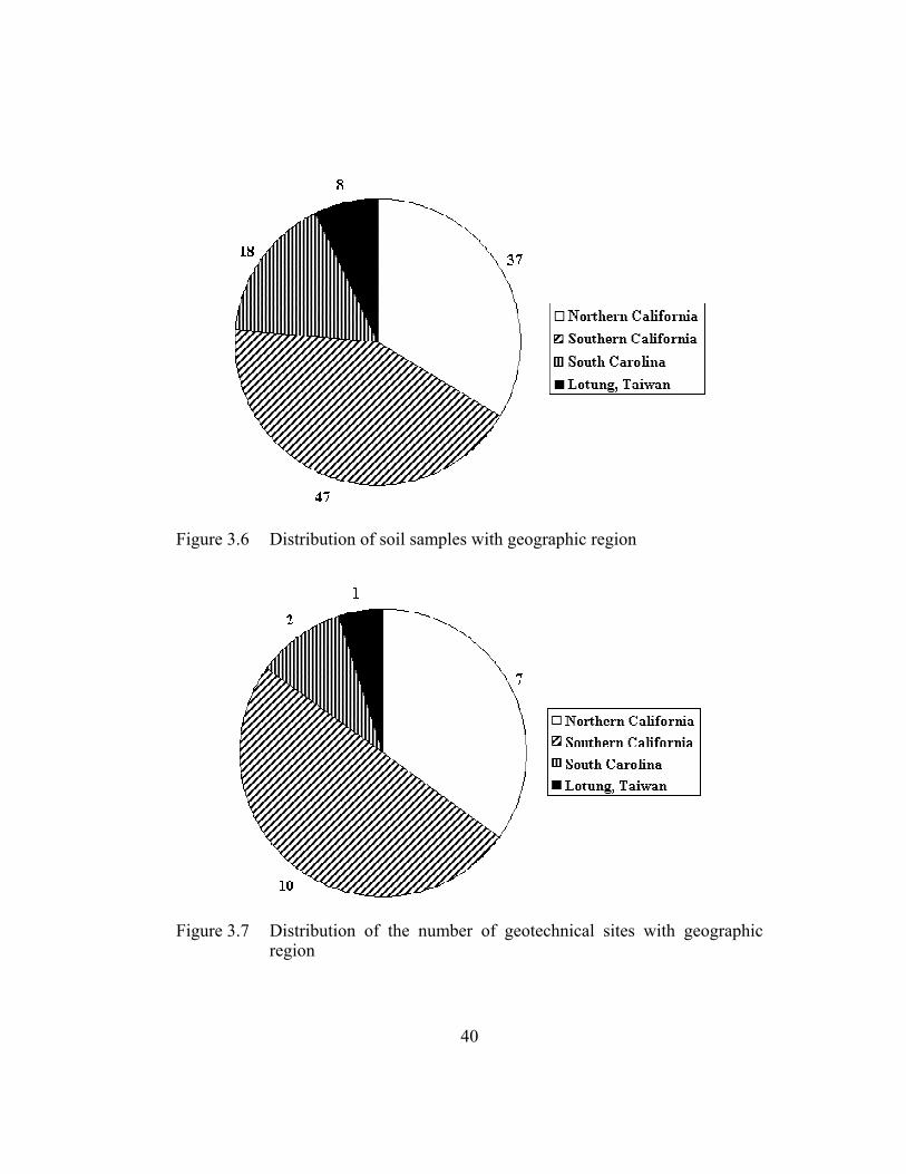
40
Figure 3.6 Distribution of soil samples with geographic region
Figure 3.7 Distribution of the number of geotechnical sites with geographic region

41
Figure 3.8 Distribution of soil samples according to the sample depth
Table 3.21 Distribution of soil samples according to the sample depth in each geographic region
Geographic Region 0-5 5-10 10-20 20-30 30-50 50-100 100-200 200-263 TOTALNorthern California 5 8 4 6 7 5 2 - 37Southern California 8 5 7 4 8 7 6 2 47
South Carolina 1 1 4 3 2 3 2 2 18Taiwan - 1 2 2 3 - - - 8TOTAL 14 15 17 15 20 15 10 4 110
Depth Range (meters)
In Figure 3.9, information regarding the isotropic confining pressures at
which nonlinear measurements have been performed is presented. The test
pressures ranged from 0.3 to 27 atmospheres. The isotropic confining test
pressure is in most cases equal to the estimated in-situ mean effective stress
calculated based on the sample depth, location of water table and assuming 0.5 as
the coefficient of horizontal earth pressure at rest. However, some specimens

42
were tested at more than one state of stress. As a result, the total number of test
pressures at which nonlinear measurements are performed is slightly more than
the total number of specimens. The number of samples from each geographic
region in each confining pressure category is presented in Table 3.22.
Figure 3.9 Distribution of confining pressures at which nonlinear measurements were performed
Table 3.22 Distribution of collected according to the isotropic confining pressure in each geographic region
Geographic Region 0.3-0.5 0.5-1.0 1.0-2.0 2.0-4.0 4.0-8.0 8.0-16.0 16.0-27.2 TOTALNorthern California 7 6 7 12 6 2 1 41Southern California 5 5 11 12 13 4 5 55
South Carolina 1 4 1 5 5 2 1 19Taiwan 1 1 3 3 - - - 8TOTAL 14 16 22 32 24 8 7 123
Test Pressure Range (atmospheres)

43
Figures 3.10 and 3.11 show the distribution of soil samples according to
the Unified Soil Classification System (USCS) designation and in terms of their
plasticity, respectively. It is important to note that soils with a wide range of
plasticity are represented in this database. About half of the soils classify as fine-
grained soils. Coarse-grained soils included in this study are limited to sands. Due
to limitations on specimen size, gravelly soils were not tested as part of this work.
The number of samples in each sample depth category divided according to their
Unified Soil Classification System (USCS) designation is presented in Table 3.23.
This table shows whether a given soil type from a given depth range is
represented in the database or not. It is important to note that a variety of soil
types from a wide range of sampling depths are represented in this database.
Figure 3.10 Distribution of soil samples according to soil type as classified by the Unified Soil Classification System (USCS)

44
Figure 3.11 Distribution of soil samples according to soil plasticity in terms of the plasticity index, PI
Table 3.23 Distribution of soil samples according to the Unified Soil Classification System (USCS) designation and sample depth
Soil Type 0-5 5-10 10-20 20-30 30-50 50-100 100-200 200-263 TOTALCH 1 1 3 3 - 1 3 - 12CL 3 5 2 1 6 6 3 2 28
CL-ML 3 - - 1 - - - - 4MH - - - 3 - - - - 3ML - 1 2 1 6 - 1 - 11SC 3 1 1 1 - - - 1 7
SC-SM - 1 - 1 - 1 1 - 4SM 3 3 7 3 4 3 1 1 25SP 1 - 1 - - - - - 2
SP-SM - 1 1 1 3 2 1 9SW-SC - 1 - - - - - - 1SW-SM - 1 - - 1 2 - - 4TOTAL 14 15 17 15 20 15 10 4 110
Depth Range (meters)
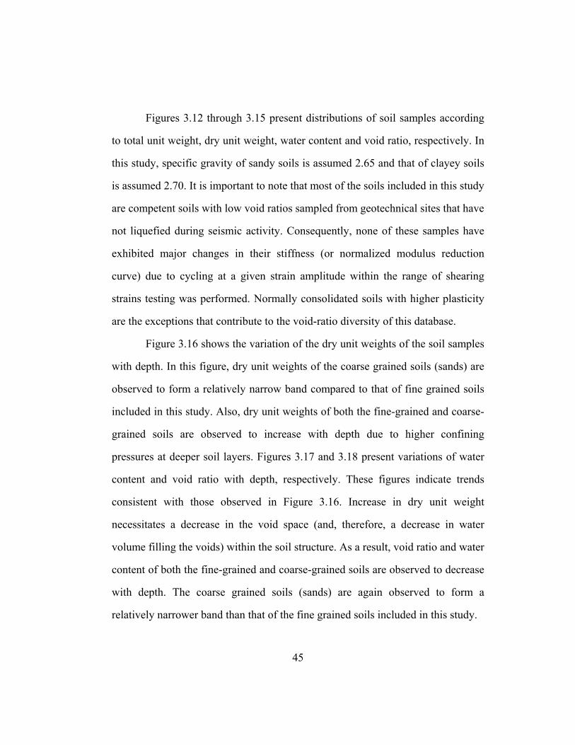
45
Figures 3.12 through 3.15 present distributions of soil samples according
to total unit weight, dry unit weight, water content and void ratio, respectively. In
this study, specific gravity of sandy soils is assumed 2.65 and that of clayey soils
is assumed 2.70. It is important to note that most of the soils included in this study
are competent soils with low void ratios sampled from geotechnical sites that have
not liquefied during seismic activity. Consequently, none of these samples have
exhibited major changes in their stiffness (or normalized modulus reduction
curve) due to cycling at a given strain amplitude within the range of shearing
strains testing was performed. Normally consolidated soils with higher plasticity
are the exceptions that contribute to the void-ratio diversity of this database.
Figure 3.16 shows the variation of the dry unit weights of the soil samples
with depth. In this figure, dry unit weights of the coarse grained soils (sands) are
observed to form a relatively narrow band compared to that of fine grained soils
included in this study. Also, dry unit weights of both the fine-grained and coarse-
grained soils are observed to increase with depth due to higher confining
pressures at deeper soil layers. Figures 3.17 and 3.18 present variations of water
content and void ratio with depth, respectively. These figures indicate trends
consistent with those observed in Figure 3.16. Increase in dry unit weight
necessitates a decrease in the void space (and, therefore, a decrease in water
volume filling the voids) within the soil structure. As a result, void ratio and water
content of both the fine-grained and coarse-grained soils are observed to decrease
with depth. The coarse grained soils (sands) are again observed to form a
relatively narrower band than that of the fine grained soils included in this study.

46
Figure 3.12 Distribution of soil samples according to total unit weight
Figure 3.13 Distribution of soil samples according to dry unit weight
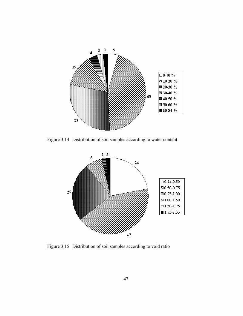
47
Figure 3.14 Distribution of soil samples according to water content
Figure 3.15 Distribution of soil samples according to void ratio

48
0
50
100
150
200
250
300
0.00 0.50 1.00 1.50 2.00 2.50
Dry Unit Weight, gr/cm3
Depth, m
(a)
Clayey SoilsSilty Soils
0.0
50.0
100.0
150.0
200.0
250.0
300.0
0.00 0.50 1.00 1.50 2.00 2.50
Dry Unit Weight, gr/cm3
Depth, m
(b)Sandy Soils
Figure 3.16 Variation of dry unit weight with depth of (a) fine grained and (b) coarse grained soils included in this study

49
0
50
100
150
200
250
300
0 20 40 60 80 100
Water Content, %
Depth, m
(a)
Clayey SoilsSilty Soils
0.0
50.0
100.0
150.0
200.0
250.0
300.0
0 20 40 60 80 100
Water Content, %
Depth, m
(b)
Sandy Soils
Figure 3.17 Variation of water content with depth of (a) fine grained and (b) coarse grained soils included in this study
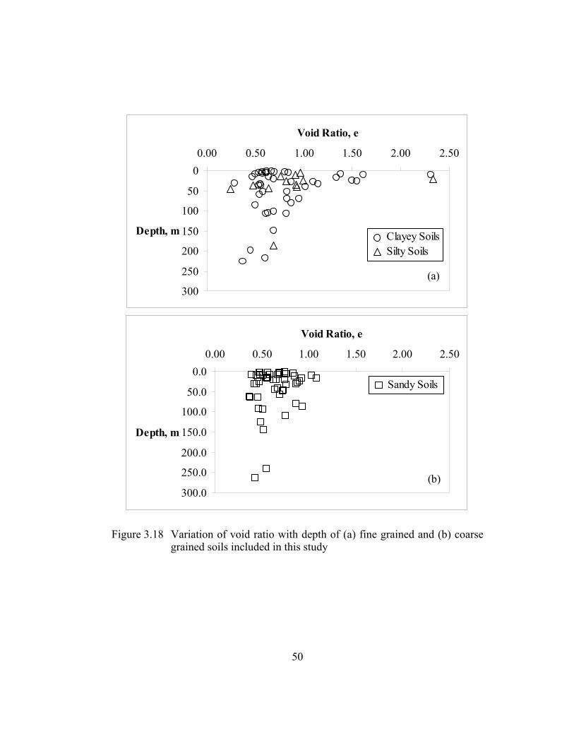
50
0
50
100
150
200
250
300
0.00 0.50 1.00 1.50 2.00 2.50
Void Ratio, e
Depth, m
(a)
Clayey SoilsSilty Soils
0.0
50.0
100.0
150.0
200.0
250.0
300.0
0.00 0.50 1.00 1.50 2.00 2.50
Void Ratio, e
Depth, m
(b)
Sandy Soils
Figure 3.18 Variation of void ratio with depth of (a) fine grained and (b) coarse grained soils included in this study
51
In Figures 3.19 and 3.20, the distribution of samples according to
estimated overconsolidation ratio and the variation of estimated overconsolidation
ratio with depth are presented, respectively. The overconsolidated soils included
in this study are observed to be sampled from depths less than about 50 m.
Unfortunately, it was not feasible to perform consolidation tests on these samples
during the course of this work. Overconsolidation ratio of the samples are
estimated based on the characteristics of log Gmax – log σo’ relationships. The
effective isotropic confining pressure, at which a break in the log Gmax – log σo’
relationship is observed, is assumed to be the maximum mean effective stress that
the sample has experienced. Overconsolidation ratio is calculated by dividing this
pressure to the estimated mean effective stress. In most cases, the soils are
classified as normally consolidated when a clean break in the log Gmax – log σo’
relationship is not observed.
Figure 3.19 Distribution of soil samples according to estimated overconsolidation ratio
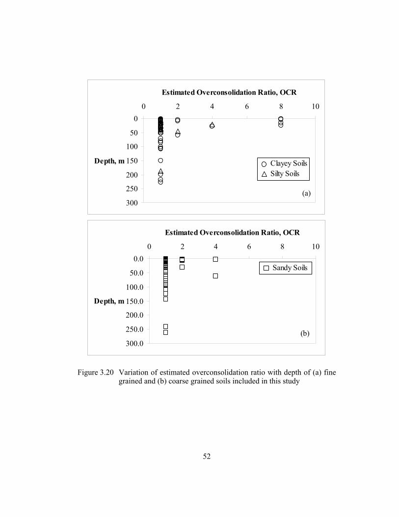
52
0
50
100
150
200
250
300
0 2 4 6 8 10
Estimated Overconsolidation Ratio, OCR
Depth, m
(a)
Clayey SoilsSilty Soils
0.0
50.0
100.0
150.0
200.0
250.0
300.0
0 2 4 6 8 10
Estimated Overconsolidation Ratio, OCR
Depth, m
(b)
Sandy Soils
Figure 3.20 Variation of estimated overconsolidation ratio with depth of (a) fine grained and (b) coarse grained soils included in this study

53
3.7 SUMMARY
The data that is analyzed in order to evaluate nonlinear soil behavior is
presented herein. This database has been compiled over the past decade from
research work supported by various organizations and carried out by a number of
graduate students working in the soil dynamics laboratory at The University of
Texas at Austin. Information regarding specimens from each geotechnical site in a
given geographic region is presented in separate tables showing physical
properties of soils and citing the publication that contains the original data.
A discussion regarding the distribution of samples in terms of their
geographic location, depth, soil type, plasticity index, void ratio and unit weight is
also presented at the end of this chapter in an attempt to familiarize the reader
with the characteristics of the database that is utilized in this study.
54
CHAPTER 4
OBSERVED TRENDS IN DYNAMIC SOIL PROPERTIES
4.1 INTRODUCTION
Dynamic soil properties (in terms of G and D) and the parameters that
affect these properties are discussed in this chapter. The relative importance of
each parameter on G and D and the trends reported in the literature and/or
observed during the course of this work are presented. This discussion is
presented so that the shortcomings of the existing empirical curves presented in
Chapter Five can be assessed and the strengths and limitations of the improved
empirical relationships developed in this study can be easily recognized.
4.2 BACKGROUND
Nonlinear dynamic soil properties are affected by a number of parameters
which have varying levels of importance. These parameters can be divided into
two groups: 1) parameters that relate to the static and dynamic loading conditions,
and 2) parameters that relate to the material type.
Important parameters related to the loading conditions which affect
nonlinear soil behavior are:
a) strain amplitude,
b) magnitude of the effective confinement state, often expressed by the
“equivalent” effective isotropic confining pressure,
c) duration of the effective confinement state, sometimes termed the
“long term time effect”,
55
d) number of loading cycles,
e) loading frequency (or strain rate), and
f) overconsolidation ratio (or loading history).
Soils are natural materials that can, and typically do, vary widely. The
behavior and performance of these materials tend to change significantly from
one soil to another. One of the challenges that a geotechnical engineer has to deal
with is the necessity to design an engineered structure with the material available
at a given site. As a result, for decades, geotechnical engineers have been
classifying different soils and associating their performance in various
applications with soil classes. This perspective has been utilized herein to analyze
the impact of material type on dynamic soil behavior. This study is an effort to
characterize nonlinear behavior of “competent” soils (soils that do not undergo
large volume changes during dynamic loading) at shearing strain amplitudes less
than 1 %. The results of this research are intended to be utilized in the analysis of
free-field ground motions during design level earthquakes.
Finally, the effect of sampling disturbance on dynamic soil properties is
briefly discussed in this chapter in order to show the importance of small-strain,
in-situ seismic measurements and to justify the emphasis in this work on
normalized modulus reduction curves rather than absolute values of stiffness.
Unfortunately, seismic methods have not been successfully used to date to
measure in-situ material damping ratio at any strain level on a routine basis.
Therefore, it is not possible to apply some type of laboratory-to-field
transformation to obtain field material damping curves. As a result, damping

56
curves measured in the laboratory are directly utilized as design curves in ground
motion analysis.
4.3 NONLINEAR DYNAMIC SOIL PROPERTIES
As discussed in Chapter One, soils exhibit nonlinear behavior. In other
words, secant shear modulus, G, decreases with increasing strain amplitude. Shear
modulus at small strains is referred to as small-strain shear modulus, Gmax or Go.
The relationship between shear modulus and shearing strain amplitude is typically
characterized by a normalized modulus reduction curve as shown in Figure 4.1a.
The nonlinearity in the stress-strain relationship results in an increase in
energy dissipation and therefore an increase in material damping ratio, D, with
increasing strain amplitude. Material damping ratio at small strains is referred to
as small-strain material damping ratio, Dmin. The relationship between material
damping ratio and strain amplitude is typically characterized by a material
damping curve as shown in Figure 4.1b. As noted above and as illustrated in
Figure 4.1b, D-log γ curve is expressed in absolute terms, not in normalized terms
(for instance D/Dmin-log γ or D/Dmax-log γ) because the nonlinear characteristics
of the D-log γ curve are related to the normalized modulus reduction curve of a
given soil rather than the value of material damping ratio at small or large strains.
These two curves can be broken into three strain ranges over which soils
behave differently. At small strains, γ < 0.001 %, soils exhibit linear elastic
behavior. The main source of energy dissipation is friction between particles
and/or viscosity. In other words, shear modulus is constant at a maximum value,
Gmax, and material damping ratio is constant at a minimum value, Dmin.

57
γte γt
c
N=10
N=11.0
0.5
00.001 0.01 0.1 1Shearing Strain, γ, %
~0.8G
Gmax
(a)
γte γt
c
D, %
16
8
00.001 0.01 0.1 1Shearing Strain, γ, %
∆D ~3 %
Dmin
(b)
γte = elastic treshold strain
γtc = cyclic treshold strain
Linear ElasticNonlinear ElasticPlastic
γte γt
c
N=10
N=11.0
0.5
00.001 0.01 0.1 1Shearing Strain, γ, %
~0.8G
Gmax
(a)
γte γt
c
N=10
N=11.0
0.5
00.001 0.01 0.1 1Shearing Strain, γ, %
~0.8G
Gmax
(a)
γte γt
c
D, %
16
8
00.001 0.01 0.1 1Shearing Strain, γ, %
∆D ~3 %
Dmin
(b)
γte γt
c
D, %
16
8
00.001 0.01 0.1 1Shearing Strain, γ, %
∆D ~3 %
Dmin
(b)
γte = elastic treshold strain
γtc = cyclic treshold strain
Linear ElasticNonlinear ElasticPlastic
γte = elastic treshold strain
γtc = cyclic treshold strain
Linear ElasticNonlinear ElasticPlastic
Linear ElasticNonlinear ElasticPlastic
Figure 4.1 Linear elastic, nonlinear elastic and plastic strain ranges on (a) normalized modulus reduction and (b) material damping curves

58
The strain amplitude at which shear modulus decreases to 98 % of its
original value is commonly called the elastic threshold strain and is denoted by etγ . It is also called the nonlinearity threshold by Vucetic and Dobry (1991) and
Ishihara (1996). Above the elastic threshold strain, soils behave nonlinear but still
elastic. In other words, the stress-strain relationship is curved, but the
deformations are recoverable upon unloading. Due to the nonlinear stress-strain
relationship, an increase in material damping ratio is observed. The strain
amplitude at which deformations become irrecoverable is called the cyclic (or
plastic) threshold strain and is denoted by ctγ . It is also called the degradation
threshold by Vucetic and Dobry (1991) and Ishihara (1996). At this strain, shear
modulus has decreased to about 80 % of Gmax, and material damping ratio is about
3 % higher than Dmin (Stokoe et al., 1999).
Above the cyclic threshold strain, soils may change volume as they
deform. Soils exhibit different behavior when sheared depending on how dense
they are packed. Loose saturated soils tend to contract and/or develop positive
pore pressures while dense soils tend to dilate and/or develop negative pore
pressures. A change in pore pressure results in a change in effective stress and
normalized modulus reduction and material damping curves shift with each cycle
of loading and unloading, as presented in Figure 4.1. Normalized modulus
reduction curves of the soils analyzed in this study were observed to shift very
little (or not at all in most cases) with number of cycles while a considerable shift
in material damping curve was recognized. The effect of number of loading
cycles on dynamic soil behavior is discussed in more detail in Section 4.7.
59
4.4 EFFECT OF DURATION OF CONFINEMENT ON SMALL-STRAIN DYNAMIC SOIL PROPERTIES
Figure 4.2 shows the effects of magnitude and duration of isotropic
confining pressure on the small-strain shear modulus and material damping ratio
for a typical soil specimen (UTA-1-J in Table 3.11). The variation of void ratio
with magnitude and duration of isotropic confining pressure is also presented in
this figure.
As shown in Figure 4.2a, Gmax increases as the specimen consolidates at a
given confining pressure and it also increases with increasing confining pressure.
As shown in Figure 4.2b, Dmin decreases as the specimen consolidates at a given
confining pressure and it also decreases with increasing confining pressure.
The impact of magnitude and duration of confining pressure is smaller if
the soil specimen is in an overconsolidated state (in other words, if the specimen
has been subjected to a higher confining pressure in the past) compared with the
normally consolidated state for all soils. Furthermore, these effects decrease as
overconsolidation ratio increases. If the soil specimen is normally consolidated,
magnitude and duration of confining pressure is observed to have a larger effect
on clayey soils than on sandy soils.
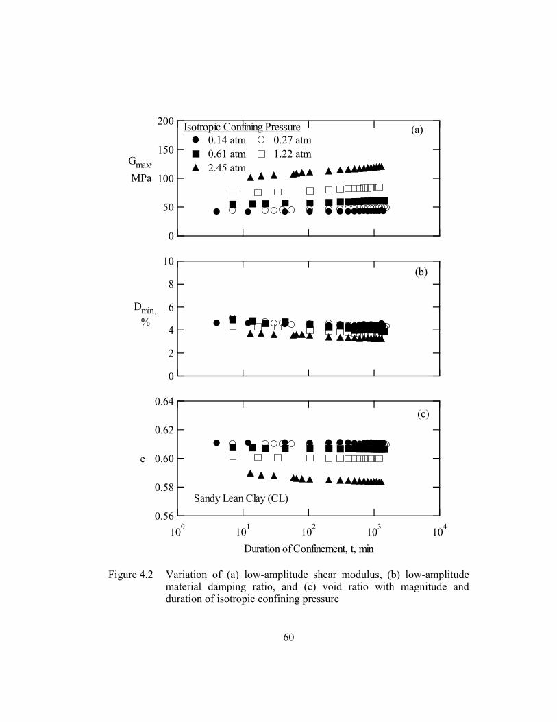
60
200
150
100
50
0
Gmax,
(a)
MPa
Isotropic Confining Pressure0.14 atm 0.27 atm0.61 atm 1.22 atm2.45 atm
10
8
6
4
2
0
Dmin,
(b)
%
0.64
0.62
0.60
0.58
0.56
e
100 101 102 103 104
Duration of Confinement, t, min
Sandy Lean Clay (CL)
(c)
Figure 4.2 Variation of (a) low-amplitude shear modulus, (b) low-amplitude material damping ratio, and (c) void ratio with magnitude and duration of isotropic confining pressure

61
The sandy lean clay (CL) specimen in Figure 4.2 is expected to reach 99%
consolidation in a fraction of the time period over which a change in small-strain
dynamic properties is observed. Part of the increase in Gmax and the decrease in
Dmin results from the consolidation of the specimen under the applied pressure.
However, small-strain dynamic properties continue to change after consolidation
of the specimen (in other words after the applied pressure has become the
effective confining pressure). The impact of duration of confining pressure after
primary consolidation is called the long-term time effect (or creep) and is
discussed in detail by Anderson and Stokoe (1978).
4.5 EFFECT OF EFFECTIVE CONFINING PRESSURE
4.5.1 Small-Strain (Linear) Dynamic Soil Properties
The effect of effective confining pressure, σo’, on small-strain dynamic
soil properties has been documented by various investigators (e.g., Hardin and
Drnevich, 1972a and b; Hardin, 1978; Stokoe et al., 1994; and Stokoe et al.,
1999). This effect is studied by measuring values of Gmax and Dmin (and void ratio
for that matter) after the specimen (UTA-1-J in Table 3.11) has fully consolidated
at each confining pressure. Typical results illustrating the effect of σo’ are
presented in Figure 4.3.
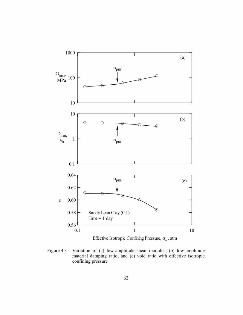
62
10
100
1000
Gmax,
(a)
MPa
σpm'
0.1
1
10
Dmin,
(b)
% σpm'
0.64
0.62
0.60
0.58
0.56
e
0.1 1 10Effective Isotropic Confining Pressure, σo
′, atm
Sandy Lean Clay (CL)Time = 1 day
(c)σpm'
Figure 4.3 Variation of (a) low-amplitude shear modulus, (b) low-amplitude material damping ratio, and (c) void ratio with effective isotropic confining pressure
63
Small-strain shear modulus, Gmax, increases with increasing effective
confining pressure as shown in Figure 4.3a. Overconsolidated soils tend to exhibit
some “memory” of stress history and they can be recognized from their bilinear
log Gmax – log σo’ relationships. The effective confining pressure at which a
change in the slope of log Gmax – log σo’ relationship is observed is the maximum
mean effective stress that the soil sample has ever experienced in the past and it is
indicated with σpm’ in Figure 4.3.
In the normally consolidated range, the slope of log Gmax – log σo’
relationship for most competent soils falls in a range of about 0.5 to 0.6. In the
overconsolidated range, Gmax is less sensitive to σo’, resulting in log Gmax – log
σo’ relationships with slopes smaller than 0.5.
Small-strain material damping ratio, Dmin, decreases with increasing
confining pressure as shown in Figure 4.3b. As in the case of Gmax,
overconsolidated soils tend to exhibit a bilinear log Dmin – log σo’ relationship. A
change in slope is observed at σpm’. The slope of log Dmin – log σo’ relationship in
the normally consolidated range is slightly higher than the slope in the
overconsolidated range. The variation of void ratio, e, with confining pressure is
also presented in Figure 4.3.
4.5.2 Nonlinear Dynamic Soil Properties
Over the past three decades, numerous studies have been conducted
regarding dynamic soil properties and the parameters affecting them. Various
investigators have synthesized this work and proposed nonlinear generic curves
for use in earthquake analyses (e.g., Seed et al., 1986, for sands, and Vucetic and

64
Dobry, 1991, for soils with plasticity). Most of these generic curves proposed in
previous studies were derived from dynamic measurements at effective confining
pressures around one atmosphere.
The importance of effective confining pressure on the variation of shear
modulus, normalized shear modulus and material damping ratio with shearing
strain is illustrated in Figure 4.4. These measurements were performed on a
normally consolidated silty sand (SM) specimen (UTA-1-M in Table 3.11). The
specimen was tested at the estimated in-situ mean effective confining pressure of
0.5 atm. Then, the confining pressure was increased to four times the estimated
in-situ mean effective confining pressure and the specimen was tested at 2.0 atm
again in a normally consolidated state. All results shown in Figure 4.4 were
determined using the resonant column method; hence, each measurement
involved about 1000 cycles of loading in the frequency range of 43 to 94 Hz. The
effect of number of cycles on dynamic soil behavior is discussed in Section 4.7.
Figure 4.4 illustrates that normalized modulus reduction and material
damping curves become increasingly linear as confining pressure increases. Only
a few investigations (e.g., Iwasaki et al., 1978; Kokusho, 1980; Ni, 1987; and
Ishibashi and Zhang, 1993) have considered the effect of confining pressure on
dynamic soil properties. However, most of these studies were restricted to
pressures much less than 10 atmospheres.

65
150
100
50
0
G, MPa
Silty Sand (SM)
(a)
1.2
0.8
0.4
0.0
G/Gmax
(b)
20
15
10
5
0
D, %
0.0001 0.001 0.01 0.1 1
Shearing Strain, γ, %
(c)σo' ~ 0.5 atmσo' ~ 2.0 atm
Figure 4.4 The effect of confining pressure on the variation of (a) shear modulus, (b) normalized shear modulus, and (c) material damping ratio with shearing strain amplitude as measured in the torsional resonant column

66
As part of the ROSRINE project, numerous intact soil samples were
recovered over a depth range of 3 to 300 m. Some of these samples were tested
using combined resonant column and torsional shear (RCTS) equipment at
isotropic confining pressures ranging from 0.25 to 30 atmospheres. The results of
these tests show that depth as manifested through confining pressure, has a
significant impact on the shear modulus, normalized modulus reduction and
material damping curves for all soils (Stokoe et al., 1999). Typical representative
results from the ROSRINE project are illustrated in Figures 4.5 and 4.6. In
Figures 4.5a and b, average normalized modulus reduction curves for soils with
moderate plasticity and for nonplastic soils are presented, respectively. In Figure
4.6, the effect of confining pressure on normalized modulus reduction and
material damping curves is illustrated based on the results of the tests performed
on silty sands. However, only general trends were noted in the ROSRINE study.
Unfortunately, a quantitative model explaining these trends was not developed.
Hence, ROSRINE project formed the foundation for this study.
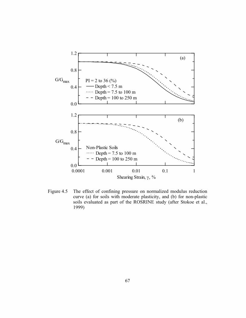
67
1.2
0.8
0.4
0.0
G/Gmax PI = 2 to 36 (%)Depth < 7.5 mDepth = 7.5 to 100 mDepth = 100 to 250 m
(a)
1.2
0.8
0.4
0.0
G/Gmax
0.0001 0.001 0.01 0.1 1Shearing Strain, γ, %
Non-Plastic SoilsDepth = 7.5 to 100 mDepth = 100 to 250 m
(b)
Figure 4.5 The effect of confining pressure on normalized modulus reduction curve (a) for soils with moderate plasticity, and (b) for non-plastic soils evaluated as part of the ROSRINE study (after Stokoe et al., 1999)
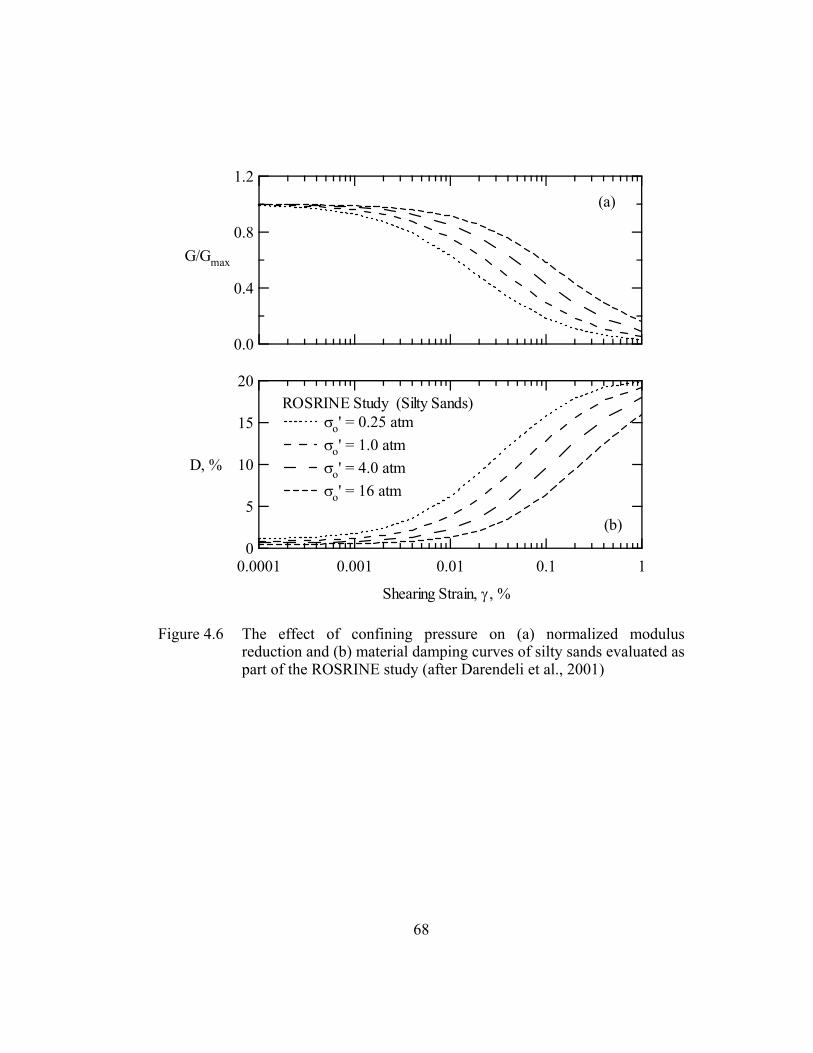
68
1.2
0.8
0.4
0.0
G/Gmax
(a)
20
15
10
5
0
D, %
0.0001 0.001 0.01 0.1 1
Shearing Strain, γ , %
(b)
ROSRINE Study (Silty Sands) σo' = 0.25 atm σo' = 1.0 atm σo' = 4.0 atm σo' = 16 atm
Figure 4.6 The effect of confining pressure on (a) normalized modulus reduction and (b) material damping curves of silty sands evaluated as part of the ROSRINE study (after Darendeli et al., 2001)
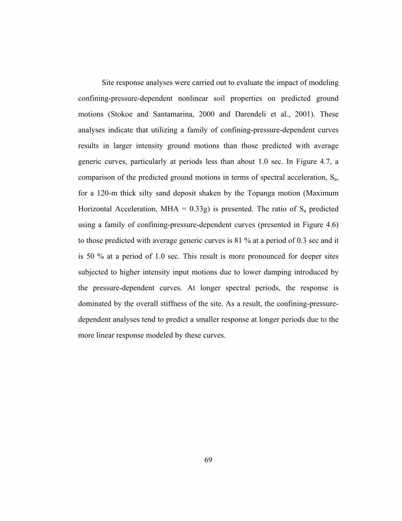
69
Site response analyses were carried out to evaluate the impact of modeling
confining-pressure-dependent nonlinear soil properties on predicted ground
motions (Stokoe and Santamarina, 2000 and Darendeli et al., 2001). These
analyses indicate that utilizing a family of confining-pressure-dependent curves
results in larger intensity ground motions than those predicted with average
generic curves, particularly at periods less than about 1.0 sec. In Figure 4.7, a
comparison of the predicted ground motions in terms of spectral acceleration, Sa,
for a 120-m thick silty sand deposit shaken by the Topanga motion (Maximum
Horizontal Acceleration, MHA = 0.33g) is presented. The ratio of Sa predicted
using a family of confining-pressure-dependent curves (presented in Figure 4.6)
to those predicted with average generic curves is 81 % at a period of 0.3 sec and it
is 50 % at a period of 1.0 sec. This result is more pronounced for deeper sites
subjected to higher intensity input motions due to lower damping introduced by
the pressure-dependent curves. At longer spectral periods, the response is
dominated by the overall stiffness of the site. As a result, the confining-pressure-
dependent analyses tend to predict a smaller response at longer periods due to the
more linear response modeled by these curves.

70
2.5
2.0
1.5
1.0
0.5
0.0
S a, g
0.01 0.1 1 10
Period, T, sec
Pressure-DependentSoil PropertiesPressure-IndependentSoil PropertiesInput Motion
5 % Structural Damping
Figure 4.7 Impact on nonlinear site response of accounting for the effect of confining pressure on dynamic soil properties (after Darendeli et al., 2001)
4.6 EFFECT OF OVERCONSOLIDATION RATIO
Overconsolidation has an effect on the dynamic properties of soils,
particularly of those with plasticity. As an example, consider the resonant column
measurements on a kaolinite specimen presented in Figures 4.8 and 4.9. This
specimen has first been consolidated at 0.34 atm, tested at confining pressures
ranging from 0.09 to 1.36 atm in a loading sequence, and then unloaded to 0.34
atm and re-tested. These tests were performed in part to investigate the impact of
overconsolidation ratio on nonlinear behavior in both the initial loading and
unloading regions.

71
10
100
1000
Gmax,
Kaolinite Specimen
*MPa
(a)
0.1
1
10
Dmin, *
* Unloading
%
(b)
0.80
0.78
0.76
0.74
0.72
0.70
e
0.01 0.1 1 10Effective Isotropic Confining Pressure, σo', atm
Note: Specimen was consolidated at 0.34 atmbefore testing.
*
(c)
Figure 4.8 The effect of overconsolidation ratio on the variation of (a) shear modulus, (b) material damping ratio, and (c) void ratio with effective isotropic confining pressure as measured in the torsional resonant column
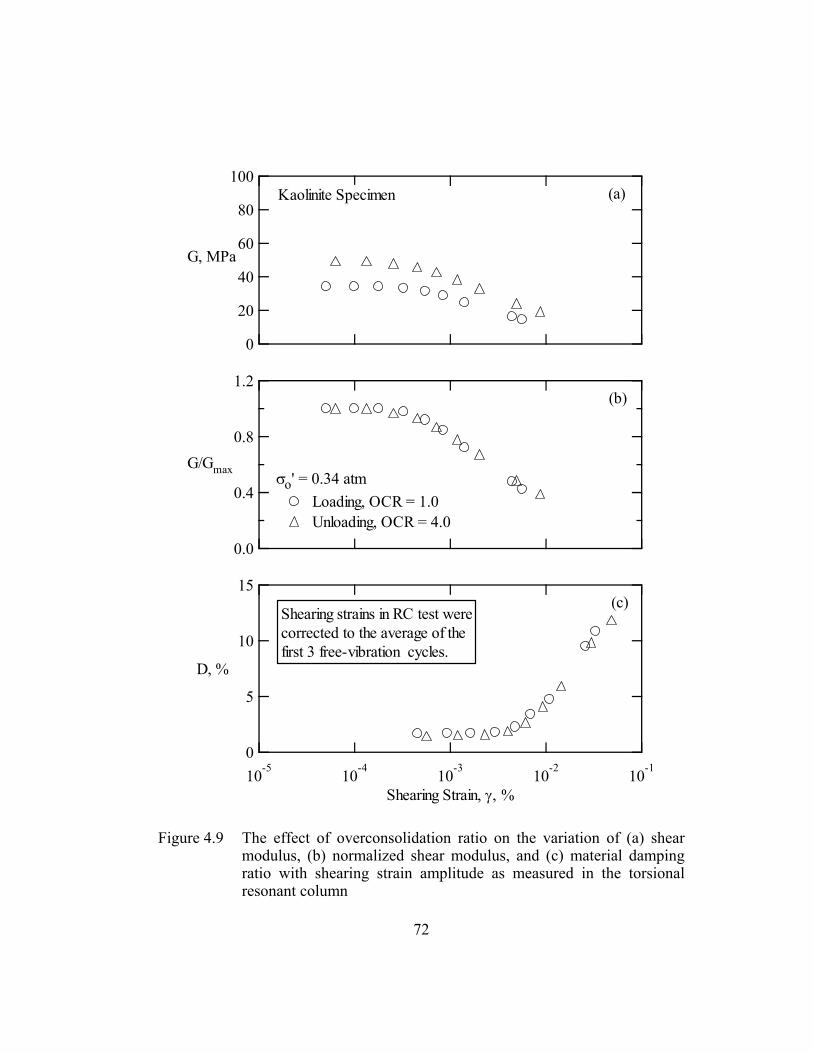
72
100
80
60
40
20
0
G, MPa
Kaolinite Specimen (a)
1.2
0.8
0.4
0.0
G/Gmaxσo' = 0.34 atm
Loading, OCR = 1.0Unloading, OCR = 4.0
(b)
15
10
5
0
D, %
10-5 10-4 10-3 10-2 10-1
Shearing Strain, γ , %
Shearing strains in RC test werecorrected to the average of thefirst 3 free-vibration cycles.
(c)
Figure 4.9 The effect of overconsolidation ratio on the variation of (a) shear modulus, (b) normalized shear modulus, and (c) material damping ratio with shearing strain amplitude as measured in the torsional resonant column

73
As illustrated in Figure 4.8 and discussed in Section 4.5, overconsolidated
soils tend to exhibit some “memory” of stress history. As a result, Gmax is larger
and Dmin is smaller in the overconsolidated state. Therefore, small-strain dynamic
properties of overconsolidated soils are less sensitive to σo’. Once a specimen is
consolidated at a higher confining pressure (back to a normally consolidated
state), a substantial decrease in void ratio results in a change in overall soil
structure and therefore a change in dynamic behavior.
The difference in Gmax for the normally consolidated and overconsolidated
states results in different nonlinear shear modulus curves as shown in Figure 4.9a.
However, in the strain range that the measurements are performed, the normalized
modulus reduction curve exhibits only a slight difference for this material as
presented in Figure 4.9b. Material damping curves for the normally consolidated
and overconsolidated states are also observed to follow a similar trend, with the
D-log γ relationship shifting slightly to higher strain amplitudes along with a
slight decrease in Dmin as shown in Figure 4.9c. Nevertheless, overconsolidation
ratio should be expected to have some impact on nonlinear soil behavior, and it
should be accounted for in developing the next generation of normalized modulus
reduction and material damping curves.
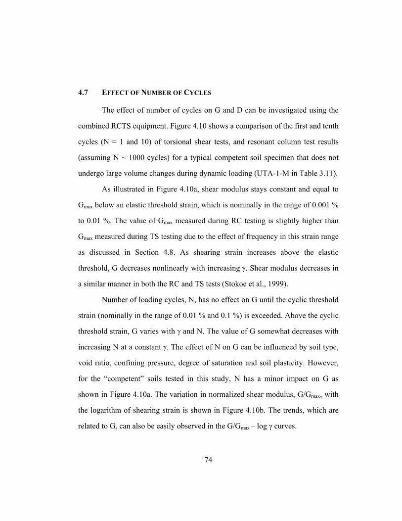
74
4.7 EFFECT OF NUMBER OF CYCLES
The effect of number of cycles on G and D can be investigated using the
combined RCTS equipment. Figure 4.10 shows a comparison of the first and tenth
cycles (N = 1 and 10) of torsional shear tests, and resonant column test results
(assuming N ~ 1000 cycles) for a typical competent soil specimen that does not
undergo large volume changes during dynamic loading (UTA-1-M in Table 3.11).
As illustrated in Figure 4.10a, shear modulus stays constant and equal to
Gmax below an elastic threshold strain, which is nominally in the range of 0.001 %
to 0.01 %. The value of Gmax measured during RC testing is slightly higher than
Gmax measured during TS testing due to the effect of frequency in this strain range
as discussed in Section 4.8. As shearing strain increases above the elastic
threshold, G decreases nonlinearly with increasing γ. Shear modulus decreases in
a similar manner in both the RC and TS tests (Stokoe et al., 1999).
Number of loading cycles, N, has no effect on G until the cyclic threshold
strain (nominally in the range of 0.01 % and 0.1 %) is exceeded. Above the cyclic
threshold strain, G varies with γ and N. The value of G somewhat decreases with
increasing N at a constant γ. The effect of N on G can be influenced by soil type,
void ratio, confining pressure, degree of saturation and soil plasticity. However,
for the “competent” soils tested in this study, N has a minor impact on G as
shown in Figure 4.10a. The variation in normalized shear modulus, G/Gmax, with
the logarithm of shearing strain is shown in Figure 4.10b. The trends, which are
related to G, can also be easily observed in the G/Gmax – log γ curves.

75
100
80
60
40
20
0
G, MPa
Silty Sand (SM) (a)
1.2
0.8
0.4
0.0
G/Gmax
(b)
Note:σm' ~ 0.5 atm
20
15
10
5
0
D, %
0.0001 0.001 0.01 0.1 1Shearing Strain, γ, %
(c)RC (~ 1000 Cycles)
TS 1st Cycle
TS 10th Cycle
Figure 4.10 The effect of number of loading cycles on the variation of (a) shear modulus, (b) normalized shear modulus, and (c) material damping ratio with shearing strain amplitude as determined in the combined RCTS testing
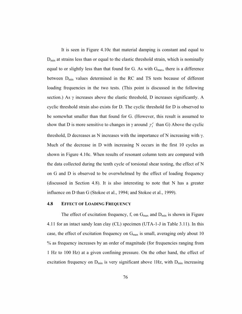
76
It is seen in Figure 4.10c that material damping is constant and equal to
Dmin at strains less than or equal to the elastic threshold strain, which is nominally
equal to or slightly less than that found for G. As with Gmax, there is a difference
between Dmin values determined in the RC and TS tests because of different
loading frequencies in the two tests. (This point is discussed in the following
section.) As γ increases above the elastic threshold, D increases significantly. A
cyclic threshold strain also exists for D. The cyclic threshold for D is observed to
be somewhat smaller than that found for G. (However, this result is assumed to
show that D is more sensitive to changes in γ around ctγ than G) Above the cyclic
threshold, D decreases as N increases with the importance of N increasing with γ.
Much of the decrease in D with increasing N occurs in the first 10 cycles as
shown in Figure 4.10c. When results of resonant column tests are compared with
the data collected during the tenth cycle of torsional shear testing, the effect of N
on G and D is observed to be overwhelmed by the effect of loading frequency
(discussed in Section 4.8). It is also interesting to note that N has a greater
influence on D than G (Stokoe et al., 1994; and Stokoe et al., 1999).
4.8 EFFECT OF LOADING FREQUENCY
The effect of excitation frequency, f, on Gmax and Dmin is shown in Figure
4.11 for an intact sandy lean clay (CL) specimen (UTA-1-J in Table 3.11). In this
case, the effect of excitation frequency on Gmax is small, averaging only about 10
% as frequency increases by an order of magnitude (for frequencies ranging from
1 Hz to 100 Hz) at a given confining pressure. On the other hand, the effect of
excitation frequency on Dmin is very significant above 1Hz, with Dmin increasing

77
by about 100 % over a log-cycle increase in excitation frequency. This effect is
clearly shown in Figure 4.11b, where all values of Dmin measured in the RC test
plot above values measured in the TS test at 1 Hz. It is also important to note that
the effect of f on Dmin is more pronounced at higher frequencies.
200
150
100
50
0
Gmax,RCTS
Isotropic Confining Pressure0.14 atm 0.27 atm0.61 atm 1.22 atm2.45 atm
(a)
MPa
10
8
6
4
2
0
Dmin, %
0.001 0.01 0.1 1 10 100 1000Loading Frequency, f, Hz
Sandy Lean Clay (CL)
RCTS
(b)
Figure 4.11 The effect of loading frequency on (a) low-amplitude shear modulus, and (b) low-amplitude material damping ratio as determined in the combined RCTS testing

78
The effect of loading frequency on Gmax and Dmin can be easily compared
when the data collected over a frequency range are normalized with the value
measured at 1 Hz. Figure 4.12 shows such a generalized summary comparison
derived from testing numerous specimens. The relative widths of the bands
indicate how much more sensitive small-strain material damping ratio is to
frequency than small-strain shear modulus.
3
2
1
0
Gmax
Gmax 1Hz
or
Dmin
D min 1Hz
0.01 0.1 1 10 100Excitation Frequency, f, Hz
D min /D min 1Hz
Gmax /Gmax 1Hz
Inc.PI
Increasing PlasticityIndex, PI
Note:Intact Specimens of Soils with PIs = 0 to 35 %
3
2
1
0
Gmax
Gmax 1Hz
or
Dmin
D min 1Hz
0.01 0.1 1 10 100Excitation Frequency, f, Hz
D min /D min 1Hz
Gmax /Gmax 1Hz
Inc.PI
Increasing PlasticityIndex, PI
Note:Intact Specimens of Soils with PIs = 0 to 35 %
Figure 4.12 Comparison of the effect of loading frequency on low-amplitude shear modulus and low-amplitude material damping ratio (from Stokoe and Santamarina, 2000)
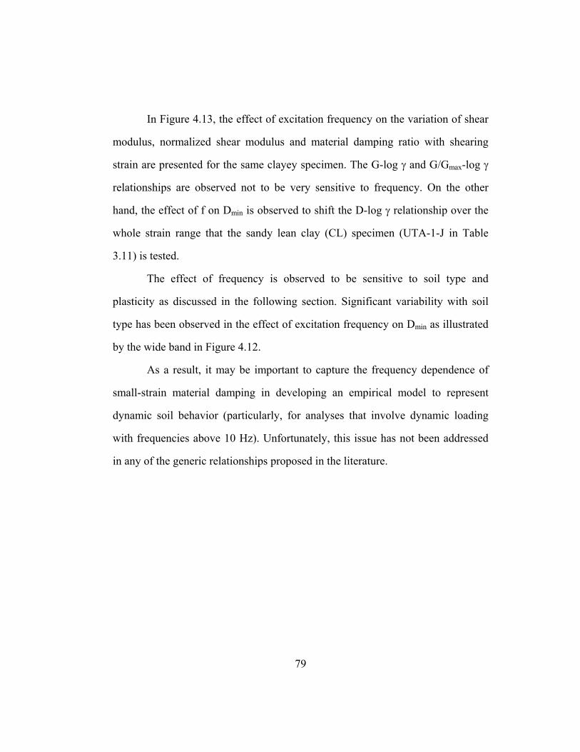
79
In Figure 4.13, the effect of excitation frequency on the variation of shear
modulus, normalized shear modulus and material damping ratio with shearing
strain are presented for the same clayey specimen. The G-log γ and G/Gmax-log γ
relationships are observed not to be very sensitive to frequency. On the other
hand, the effect of f on Dmin is observed to shift the D-log γ relationship over the
whole strain range that the sandy lean clay (CL) specimen (UTA-1-J in Table
3.11) is tested.
The effect of frequency is observed to be sensitive to soil type and
plasticity as discussed in the following section. Significant variability with soil
type has been observed in the effect of excitation frequency on Dmin as illustrated
by the wide band in Figure 4.12.
As a result, it may be important to capture the frequency dependence of
small-strain material damping in developing an empirical model to represent
dynamic soil behavior (particularly, for analyses that involve dynamic loading
with frequencies above 10 Hz). Unfortunately, this issue has not been addressed
in any of the generic relationships proposed in the literature.

80
100
80
60
40
20
0
G, MPa
Sandy Lean Clay (CL)
(a)
1.2
0.8
0.4
0.0
G/Gmax
(b)
Note:σm' ~ 0.5 atm
20
15
10
5
0
D, %
0.0001 0.001 0.01 0.1 1
Shearing Strain, γ, %
(c)RC (~ 1000 Cycles)
TS 1st Cycle
TS 10th Cycle
Figure 4.13 The effect of loading frequency on the variation of (a) shear modulus, (b) normalized shear modulus, and (c) material damping ratio with shearing strain amplitude as determined in the combined RCTS testing

81
4.9 EFFECT OF SOIL TYPE
The effect of soil type is very important when considering linear and
nonlinear dynamic soil properties as discussed in Sections 4.9.1 and 4.9.2,
respectively. This effect also manifests itself in influencing the relative effect of
other parameters such as loading frequency, number of cycles, etc. as discussed
below.
4.9.1 Small-Strain Dynamic Soil Properties
Figure 4.14 shows a comparison of the variation in Gmax and Dmin with
effective isotropic confining pressure from RCTS testing of two specimens at
similar confining pressures. One of the specimens is a silty sand (SM) specimen
(UTA-1-M in Table 3.11) and the other is a sandy lean clay (CL) specimen
(UTA-1-J in Table 3.11).
As shown in Figure 4.14a, the sandy lean clay (CL) exhibits a memory of
loading history characterized by the bilinear log Gmax – log σo’ relationship while
the silty sand (SM) follows almost a straight line. RC and TS test results denoted
with solid and open symbols in this figure are observed to be very close. This
figure also confirms that Gmax is not very sensitive to excitation frequency.
On the other hand, the values of Dmin in the log Dmin – log σo’
relationships presented in Figure 4.14b are quiet different for the two material
types. The sandy lean clay (CL) has much higher damping than the silty sand
(SM). This finding is consistent with the general trends reported in the literature
such that small-strain material damping increases with increasing soil plasticity
(Stokoe et al., 1994; and Stokoe et al., 1999).

82
10
100
1000
G,
RC TS Soil TypeSilty Sand (SM)Sandy Lean Clay (CL)
(a)
MPa
0.1
1
10
Dmin ,%
0.1 1 10Effective Isotropic Confining Pressure, σo', atm
(b)
Figure 4.14 The effect of soil type on the variation of (a) low-amplitude shear modulus, and (b) low-amplitude material damping ratio with effective isotropic confining pressure as determined in the combined RCTS testing
Unfortunately, most of the generic curves used in state of practice (e.g.,
Vucetic and Dobry, 1991) are not accurate in terms of representing this trend in
Dmin. These generic curves were synthesized from studies generally performed
with relatively older cyclic testing equipment. Because of accuracy problems at
small strains, damping measurements were not performed and data were
extrapolated to represent the small-strain behavior.

83
It is also important to note that the Dmin values measured in the RC and TS
tests are observed to be quite different for both of these materials. This is due to
the effect of excitation frequency as discussed in Section 4.8. The effect of
frequency is more pronounced on the sandy lean clay (CL). Strain-rate effects
being more pronounced in plastic soils is a well-known phenomenon reported in
the geotechnical engineering literature.
Figures 4.15 and 4.16 show the impact of excitation frequency for these
two soils in more detail. Results of torsional shear tests performed at several
frequencies well below resonance and resonant column tests performed at a
relatively higher frequency are presented for the sandy lean clay (CL) and for the
silty sand (SM) in these figures.
Figures 4.15a and 4.16a show the Gmax and Dmin measurements,
respectively, while Figures 4.15b and 4.16b present the same data using a
different perspective. The data in Figures 4.15b and 4.16b have been normalized
with the TS measurements at 1Hz in order to indicate the sensitivity of the small-
strain dynamic properties to excitation frequency.
It is important to note the scales used in Figures 4.15b and 4.16b. An
increase in Gmax on the order of 5 % to 10 % is observed per order of magnitude
increase in frequency (between 10 Hz and 100 Hz) for the silty sand (SM) and the
sandy lean clay (CL), respectively. On the other hand, an increase in Dmin on the
order of 80 % to 120 % is presented in Figure 4.16b over the same frequency
range.
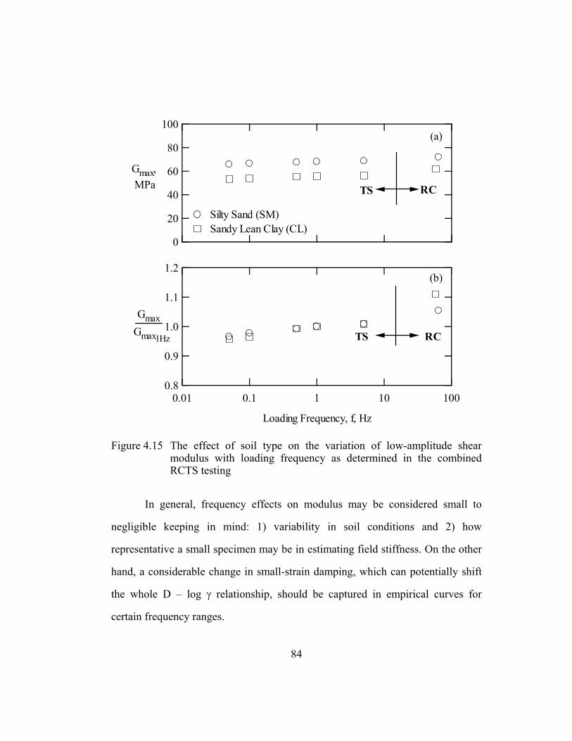
84
100
80
60
40
20
0
Gmax,
Silty Sand (SM)Sandy Lean Clay (CL)
RCTS
(a)
MPa
1.2
1.1
1.0
0.9
0.8
Gmax
0.01 0.1 1 10 100
Loading Frequency, f, Hz
RCTS
(b)
Gmax1Hz
Figure 4.15 The effect of soil type on the variation of low-amplitude shear modulus with loading frequency as determined in the combined RCTS testing
In general, frequency effects on modulus may be considered small to
negligible keeping in mind: 1) variability in soil conditions and 2) how
representative a small specimen may be in estimating field stiffness. On the other
hand, a considerable change in small-strain damping, which can potentially shift
the whole D – log γ relationship, should be captured in empirical curves for
certain frequency ranges.
85
5
4
3
2
1
0
Dmin ,%
Silty Sand (SM)Sandy Lean Clay (CL)
RCTS
(a)
3
2
1
0
Dmin
0.01 0.1 1 10 100
Loading Frequency, f, Hz
RCTS
(b)
Dmin1Hz
Figure 4.16 The effect of soil type on the variation of low-amplitude material damping ratio with loading frequency as determined in the combined RCTS testing
4.9.2 Nonlinear Dynamic Soil Properties
In terms of nonlinear soil behavior, the G/Gmax – log γ and D – log γ
curves for the SM and CL specimens discussed in the previous section are shown
in Figures 4.17 and 4.18. The comparison of the nonlinear behavior of the two
soils does not represent a wide range of soil types. However, Figure 4.17 indicates
a shift in normalized modulus reduction curve with changing soil type.
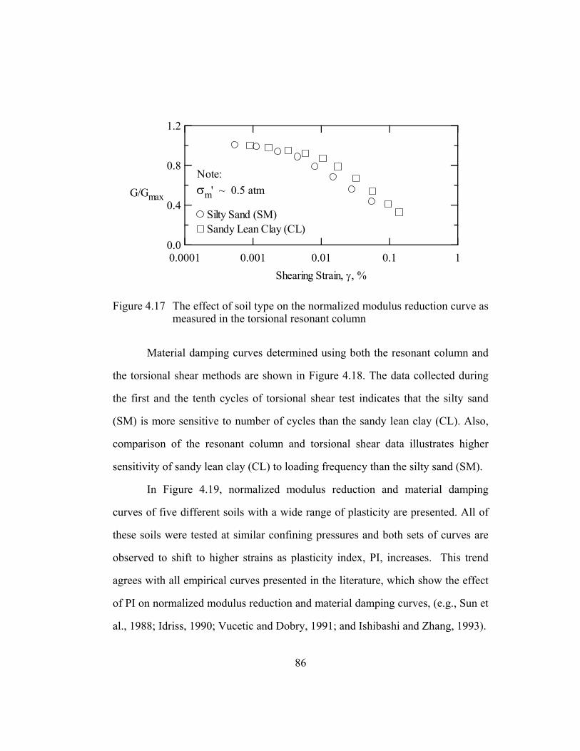
86
1.2
0.8
0.4
0.0
G/Gmax
0.0001 0.001 0.01 0.1 1Shearing Strain, γ, %
Silty Sand (SM)Sandy Lean Clay (CL)
Note:σm' ~ 0.5 atm
Figure 4.17 The effect of soil type on the normalized modulus reduction curve as measured in the torsional resonant column
Material damping curves determined using both the resonant column and
the torsional shear methods are shown in Figure 4.18. The data collected during
the first and the tenth cycles of torsional shear test indicates that the silty sand
(SM) is more sensitive to number of cycles than the sandy lean clay (CL). Also,
comparison of the resonant column and torsional shear data illustrates higher
sensitivity of sandy lean clay (CL) to loading frequency than the silty sand (SM).
In Figure 4.19, normalized modulus reduction and material damping
curves of five different soils with a wide range of plasticity are presented. All of
these soils were tested at similar confining pressures and both sets of curves are
observed to shift to higher strains as plasticity index, PI, increases. This trend
agrees with all empirical curves presented in the literature, which show the effect
of PI on normalized modulus reduction and material damping curves, (e.g., Sun et
al., 1988; Idriss, 1990; Vucetic and Dobry, 1991; and Ishibashi and Zhang, 1993).

87
20
15
10
5
0
D, %
Silty Sand (SM)Sandy Lean Clay (CL)
(a)
RC Test
20
15
10
5
0
D, %
(b)
Note:σm' ~ 0.5 atm
TS Test 1st Cyclef = 1 Hz
20
15
10
5
0
D, %
0.0001 0.001 0.01 0.1 1
Shearing Strain, γ, %
(c)TS Test 10th Cyclef = 1 Hz
Figure 4.18 The effect of soil type on the material damping curve determined at (a) N ~ 1000 cycles, (b) N = 1 cycle, and (c) N = 10 cycles from combined RCTS testing
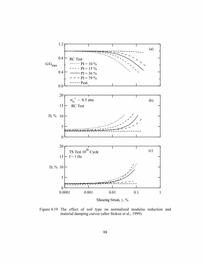
88
1.2
0.8
0.4
0.0
G/Gmax
RC TestPI = 10 %PI = 15 %PI = 36 %PI = 79 %Peat
(a)
20
15
10
5
0
D, %
(b)σm' ~ 0.5 atmRC Test
20
15
10
5
0
D, %
0.0001 0.001 0.01 0.1 1
Shearing Strain, γ, %
(c)TS Test 10th Cyclef = 1 Hz
Figure 4.19 The effect of soil type on normalized modulus reduction and material damping curves (after Stokoe et al., 1999)
89
The values of Dmin increase with increasing PI as presented in Figure 4.19.
On the other hand, the values of D at high strains (γ ~ 0.1 %) decrease as PI
increases also as shown in this figure. This rather complex relationship between
the D - log γ curves for different soils is not shown in any empirical curves. It has
been presented in a general sense in Electric Power Research Institute, EPRI
(1993b and c), based on RCTS tests of intact soil specimens tested at UT. This
behavior has also been observed by Vucetic et al. (1998) following the EPRI
study.
The general switching in the relative positions of the D- log γ curves for
the different soil types is best shown in the TS tests at an excitation frequency of 1
Hz. The effect of excitation frequency impacts the RC measurements and the
effect of number of loading cycles impacts the tenth-cycle TS measurements.
The effect of σο’ on the normalized modulus reduction and material
damping curves is discussed in Section 4.5. The general trend shows both of the
curves shifting to higher strains. In case of D - log γ relationships, the curves
simultaneously shift downward. As a result, D decreases slightly at a given γ as
σο’ increases. In general terms, the largest shift is shown by nonplastic soils, with
the effect decreasing with increasing plasticity (Stokoe et al., 1994; and Stokoe et
al., 1999). Similar behavior is observed for normalized shear modulus, except no
shift occurs at small strains with increasing σο’ because the curve is normalized
with Gmax.
90
4.10 EFFECT OF SAMPLE DISTURBANCE
Although laboratory testing methods have been standardized and
laboratory testing equipment has been significantly improved over the past several
decades, estimating accurate engineering properties of soils has always been and
will always be a challenge for geotechnical engineers. The data collected in the
laboratory should always be evaluated in terms of its success in representing the
in-situ conditions. Beside scaling effects (due to characterizing a soil deposit with
specimens that are only a few 100 cubic centimeters in volume), effects of the
sampling operation on the laboratory measurements of an engineering property
have to be taken into account prior to utilizing a laboratory test result in design.
4.10.1 Effect of Disturbance on Gmax = ρVs2
Figure 4.20 shows the shear-wave velocity measurements at one of the
sites (La Cienega located in West Hollywood) characterized as part of the
ROSRINE project. Two sets of data are presented in this figure: 1) in-situ seismic
(OYO logger and crosshole) measurements, and 2) laboratory measurements.
Comparison of the two sets of data clearly shows a discrepancy between field and
laboratory values of shear wave velocity, Vs, with laboratory Vs values generally
lower than the field measurements.
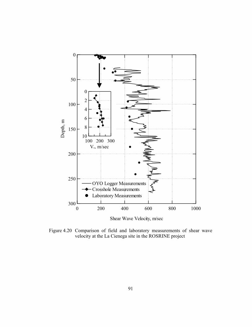
91
300
250
200
150
100
50
0D
epth
, m
10008006004002000
Shear Wave Velocity, m/sec
OYO Logger MeasurementsCrosshole MeasurementsLaboratory Measurements
Figure 4.20 Comparison of field and laboratory measurements of shear wave velocity at the La Cienega site in the ROSRINE project
10
8
6
4
2
0
300200100
Vs, m/sec
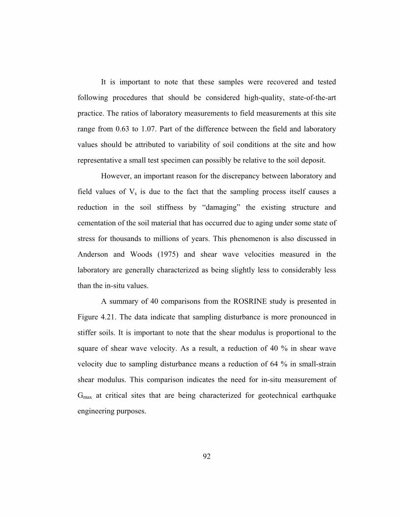
92
It is important to note that these samples were recovered and tested
following procedures that should be considered high-quality, state-of-the-art
practice. The ratios of laboratory measurements to field measurements at this site
range from 0.63 to 1.07. Part of the difference between the field and laboratory
values should be attributed to variability of soil conditions at the site and how
representative a small test specimen can possibly be relative to the soil deposit.
However, an important reason for the discrepancy between laboratory and
field values of Vs is due to the fact that the sampling process itself causes a
reduction in the soil stiffness by “damaging” the existing structure and
cementation of the soil material that has occurred due to aging under some state of
stress for thousands to millions of years. This phenomenon is also discussed in
Anderson and Woods (1975) and shear wave velocities measured in the
laboratory are generally characterized as being slightly less to considerably less
than the in-situ values.
A summary of 40 comparisons from the ROSRINE study is presented in
Figure 4.21. The data indicate that sampling disturbance is more pronounced in
stiffer soils. It is important to note that the shear modulus is proportional to the
square of shear wave velocity. As a result, a reduction of 40 % in shear wave
velocity due to sampling disturbance means a reduction of 64 % in small-strain
shear modulus. This comparison indicates the need for in-situ measurement of
Gmax at critical sites that are being characterized for geotechnical earthquake
engineering purposes.

93
900
600
300
0
1.50.50.0
0.25 1.00 2.000.10 0.50 0.80 1.50
Modulus Ratio, Gmax, lab / Gmax, fieldV
S, fi
eld,
m/s
ec
Velocity Ratio, VS, lab / VS, field
Range fromROSRINE
Study
General Trend
1.0900
600
300
0
1.50.50.0
0.25 1.00 2.000.10 0.50 0.80 1.50
Modulus Ratio, Gmax, lab / Gmax, fieldV
S, fi
eld,
m/s
ec
Velocity Ratio, VS, lab / VS, field
Range fromROSRINE
Study
General Trend
1.0
Figure 4.21 Variation of sampling disturbance expressed in terms of Vs, lab/Vs, field and Gmax, lab/Gmax, field with the in-situ shear wave velocity
4.10.2 Effect of Disturbance on Dmin
Theoretically, it is possible to estimate the small-strain material damping
ratio from in-situ seismic measurements. Crosshole and downhole test results may
be used to evaluate the in-situ material damping ratio. The SASW method may be
extended to permit in-situ measurements of material damping ratio in addition to
shear wave velocity (Lai and Rix, 1998; and Rix et al., 2000). Response of
instrumented soil deposits to earthquakes and aftershocks can be analyzed in
order to estimate in-situ shear wave velocity and material damping ratio.
However, the accuracy of all of these methods is still questionable and no robust
field method exists today.

94
Most of these methods typically assume a horizontally layered system and
utilize attenuation of wave amplitude with distance from the source.
Backscattering of waves due to the contrast between soil layers and lateral
variability in the soil deposit causes significant uncertainty regarding the
estimates of in-situ material damping ratio. The quality of the estimate is further
reduced by geometric attenuation, which generally has a more significant impact
on attenuation with distance than material damping ratio.
As an example, Figure 4.22 shows independent measurements of material
damping ratio from field and laboratory tests. These field crosshole measurements
and the laboratory measurements were conducted by UT personnel (Fuhriman,
1993; and Hwang, 1997) and are presented in EPRI (1993a and b) along with a
discussion of the data collection and analysis procedures. The material damping
ratios from surface wave measurements were performed by Lai and Rix (1998)
and are generally less than those from crosshole testing possibly due to: 1)
different attenuation mechanisms which control at higher frequencies and produce
frequency-dependent damping ratios, 2) different volumes of soil sampled by the
methods, and 3) uncoupled analyses of Vs and Dmin. On the other hand, values of
damping ratio from the surface wave tests agree more closely with values from
resonant column and torsional shear laboratory tests than those estimated using
the crosshole method. These results seem to indicate that laboratory estimates of
Dmin can be used with some “judgment” for evaluation of soil deposits for
geotechnical earthquake engineering purposes. However, many more studies are
warranted in this area.

95
Damping Ratio, %
0
3
6
9
12
0 2 4 6 8 10
Surface WaveCrosshole (UT)Resonant Column (UT)Torsional Shear (UT)
Depth, m
Damping Ratio, %
0
3
6
9
12
0 2 4 6 8 10
Surface WaveCrosshole (UT)Resonant Column (UT)Torsional Shear (UT)
Depth, m
Figure 4.22 Comparison of laboratory and field measurements of small strain material damping ratio (from Stokoe et al., 1999)
4.10.3 Effect of Disturbance on Nonlinear Behavior
4.10.3.1 Comparison of Back-calculated Curves with Laboratory Test Results
Zeghal et al. (1995) back-calculated the variations of shear modulus and
material damping ratio with shearing strain amplitude using stress-strain histories
calculated from the free-field downhole accelerations at the Lotung site in Taiwan
from which specimens discussed in Section 3.5 were taken. The comparison of
the back-calculated nonlinear soil properties with the data collected at the
University of Texas at Austin is presented in Figure 4.23.
96
(a)(a)
(b)(b)
Figure 4.23 Comparison of nonlinear soil properties back-calculated from the free-field downhole accelerations with the laboratory measurements (from Zeghal et al., 1995)
Estimates before peak shearing strain
Statistical Fit

97
Figure 4.23a indicates a good correlation between the normalized modulus
reduction curves estimated based on in-situ seismic response and the data
collected in the laboratory. There is a significant difference between the “field”
and laboratory material damping curves in Figure 4.23b. It is felt that this
difference can be attributed to different attenuation mechanisms and different
volumes of soil sampled by the two methods. However, if these curves were
utilized in ground motion analysis for earthquake resistant design, it is important
to note that the material damping curve measured in the laboratory would result in
a more conservative design than the field estimate.
4.10.3.2 Comparison of Test Results on Intact and Reconstituted Specimens
Disturbance was defined above as “damaging” the existing structure and
cementation of the soil material that has been aging under some state of stress for
thousands to millions of years. A similar process can be simulated in the
laboratory by breaking an “undisturbed” soil sample into small pieces, destroying
the existing soil structure completely and reconstituting it. This extreme situation
associated with disturbance is called remolding. Comparison of the measurements
on undisturbed and remolded soils can be utilized as an indicator of the sensitivity
to disturbance of a given engineering property for a given soil type.
98
As an example, consider the comparisons of dynamic soil properties
shown in Figures 4.24 and 4.25. In these figures, data collected from RCTS
testing of an undisturbed specimen and a remolded specimen are presented. The
first specimen was trimmed from a poorly graded sand (SP-SM) sample from
Idaho Falls (Stokoe et al., 1998c). Then, this specimen was remolded and a
second specimen was reconstituted from this material at a similar unit weight.
In Figure 4.24, the variations of small-strain shear modulus, small-strain
material damping ratio and void ratio are presented. The values of Gmax and Dmin
are observed to exhibit very similar relationships although this comparison
represents an extreme case of disturbance. Gmax values at lower confining
pressures are smaller for the remolded specimen since the undisturbed specimen
has some “memory” of state of stress in the field which is characterized by the
bilinear log Gmax – log σo’ relationship. Dmin values are quite similar (considering
the limited accuracy of damping measurements, they are essentially identical).
Figure 4.25 shows the comparison of the nonlinear soil behavior of the
undisturbed and remolded specimens at a mean effective confining pressure of
0.82 atm. About 20 % difference between the shear modulus of the undisturbed
and remolded specimens is easily recognized in Figure 4.25a at small-strain
amplitudes. On the other hand, the normalized modulus reduction curves
(presented in Figure 4.25b) for these two specimens are almost identical. The D –
log γ relationship (shown in Figure 4.25c) is nearly the same up to γ of about 0.01
%. At higher strains, the reconstituted specimen exhibits increasingly higher
values of D.

99
10
100
1000
Gmax,
MPa
(a)
0.1
1
10
Dmin, Poorly Graded Sandwith Silt (SP-SM)
Intact (γ t = 1.64 gr/cm3)
Reconstituted (γ t = 1.65 gr/cm3)
%
(b)
0.8
0.7
0.6
0.5
0.4
e
0.1 1 10Effective Isotropic Confining Pressure, σo
′, atm
(c)
Figure 4.24 Comparison of the variation of (a) low-amplitude shear modulus, (b) low-amplitude material damping ratio, and (c) void ratio with effective isotropic confining pressure of intact (undisturbed) and reconstituted (remolded) specimens

100
200
150
100
50
0
G, MPa
(a)
σo' = 0.82 atm
1.2
0.8
0.4
0.0
G/Gmax
(b)
20
15
10
5
0
D, %
10-5 10-4 10-3 10-2 10-1 100
Shearing Strain, γ, %
Poorly Graded Sandwith Silt (SP-SM)
Intact (γ t = 1.64 gr/cm3)
Reconstituted (γ t = 1.65 gr/cm3)
(c)
Figure 4.25 Comparison of the variation of (a) shear modulus, (b) normalized shear modulus, and (c) material damping ratio with shearing strain of intact (undisturbed) and reconstituted (remolded) specimens

101
4.10.3.3 Comparison of Test Results on Companion Specimens
As part of the ROSRINE project, companion samples from a site in
Southern California (La Cienega) were tested at the University of California at
Los Angeles (UCLA) and the University of Texas at Austin (UT).
Test results in terms of the shear modulus, normalized modulus reduction
and material damping curves are presented in Figure 4.26. The double-specimen
direct simple shear, DSDSS, (Doroudian and Vucetic, 1995) tests were performed
by Prof. Vucetic and students at UCLA. These results are shown by the solid
symbols in this figure. The resonant column and torsional shear test results
performed at UT are shown by open symbols. The value of shear modulus
estimated based on the in-situ seismic crosshole measurements by UT personnel
is also presented in Figure 4.26a for comparison purposes.
Each UCLA and UT companion specimen was recovered from the same
undisturbed sample, and each companion specimen was tested at equivalent
effective stresses based on an effective coefficient of earth pressure at rest of
about 0.5. It is important to note that the RCTS and DSDSS confinement states
are isotropic and anisotropic, respectively.

102
120
80
40
0
G, MPa
RC (UT)TS (UT)DSDSS (UCLA)CrossholeSeismic (UT)
(a)
1.2
0.8
0.4
0.0
G/Gmax
(b)
Equivalent σo' ~ 1.1 atm
20
15
10
5
0
D, %
0.0001 0.001 0.01 0.1 1 10
Shearing Strain, γ , %
(c)Silty Sand (SM)
Figure 4.26 Comparison of the variation of (a) shear modulus, (b) normalized shear modulus, and (c) material damping ratio with shearing strain measured using various equipment on companion soil samples (from Stokoe et al., 1999)

103
The main difference between the results from the tests performed on
companion specimens exists in shear modulus. The G/Gmax – log γ relationships
are nearly identical as are the D - log γ relationships from RCTS and DSDSS
testing. The in-situ seismic value of Gmax is above values determined in the
laboratory due to sampling disturbance. In this case, the field value is about 50%
greater than the average value determined in the laboratory. Figure 4.26 shows
that normalized modulus reduction and material damping curves fall on top of
each other for the two tests with different stress states. These data seem to
indicate that as long as a soil specimen is tested at the in-situ mean effective
confining pressure, the nonlinear soil behavior (characterized by normalized
modulus reduction and material damping curves) should be determined with
reasonable precision even though the anisotropic state of stress in the field is not
duplicated. Thus, RCTS testing under isotropic confinement is a robust means of
characterizing nonlinear soil behavior.
4.10.3.4 Final Remarks on Effects of Disturbance
At this point in time, it is not possible to conduct field measurements to
evaluate shear modulus and material damping at working strains during design
level ground shaking. The data presented in this section strongly support the state-
of-practice of scaling normalized modulus reduction curve from laboratory with
in-situ Gmax. The state-of-practice of utilizing the laboratory material damping
curve without any modification obviously needs more investigation and should be
used prudently at this time.
104
However, a geotechnical engineer always has to consider the
consequences of attempting to estimate engineering properties from small
samples. Problems associated with in-situ seismic testing (backscattering of
waves due to the contrast between soil layers and lateral variability in the soil
deposit) are not errors in testing procedures. These phenomena are a part of the
dynamic response of a soil deposit too complex (and therefore too expensive) to
model in most geotechnical investigations. A discrepancy will always exist
between a model based on engineering properties measured in the laboratory and
actual field performance. Not being able to model some phenomenon does not
endorse ignoring it. Instead, the engineer has to overcome such challenges by
using judgment based on facts and experience.
4.11 SUMMARY
In this chapter, dynamic soil properties (G and D) and parameters that
affect them are discussed. Table 4.1 shows a list of these parameters and their
relative importance in terms of affecting normalized modulus reduction and
material damping curves. Trends reported in the literature and observations made
during the course of this work are summarized. The importance of accounting for
the impact of soil type and loading conditions in developing a new generation of
design curves is addressed.
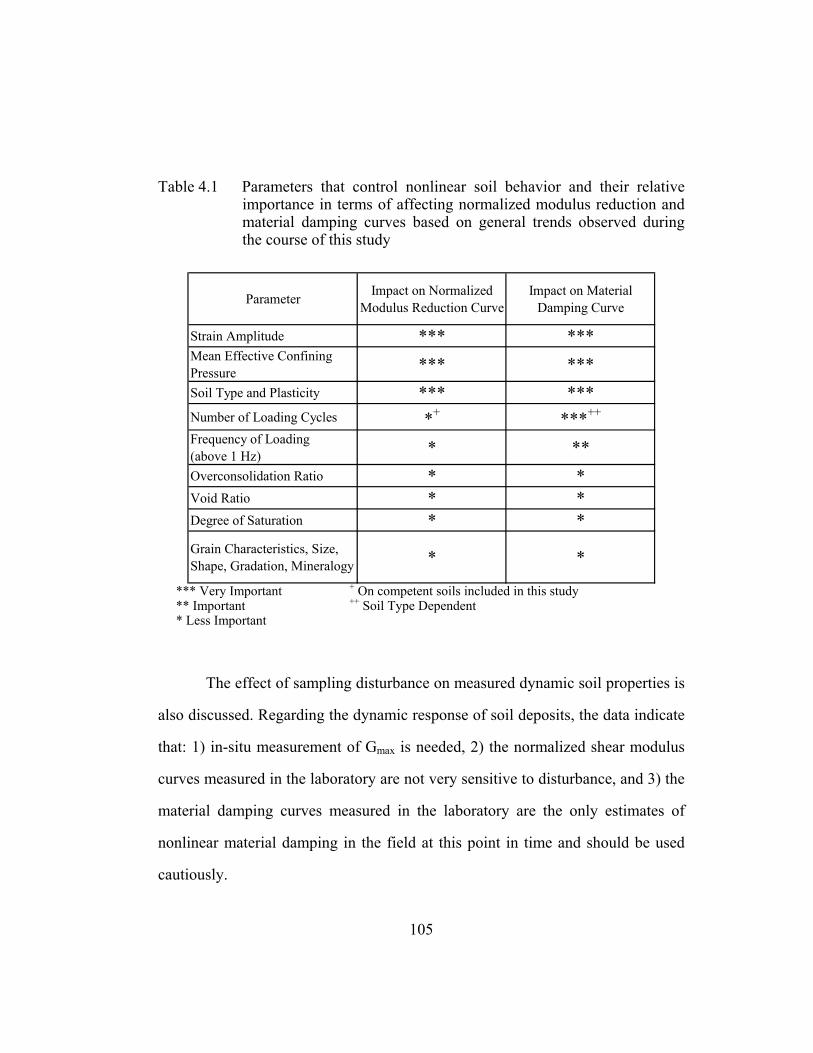
105
Table 4.1 Parameters that control nonlinear soil behavior and their relative importance in terms of affecting normalized modulus reduction and material damping curves based on general trends observed during the course of this study
Parameter Impact on Normalized Modulus Reduction Curve
Impact on Material Damping Curve
Strain Amplitude *** ***Mean Effective Confining Pressure *** ***Soil Type and Plasticity *** ***Number of Loading Cycles *+ ***++
Frequency of Loading (above 1 Hz) * **Overconsolidation Ratio * *Void Ratio * *Degree of Saturation * *Grain Characteristics, Size, Shape, Gradation, Mineralogy * *
*** Very Important + On competent soils included in this study ** Important ++ Soil Type Dependent * Less Important
The effect of sampling disturbance on measured dynamic soil properties is
also discussed. Regarding the dynamic response of soil deposits, the data indicate
that: 1) in-situ measurement of Gmax is needed, 2) the normalized shear modulus
curves measured in the laboratory are not very sensitive to disturbance, and 3) the
material damping curves measured in the laboratory are the only estimates of
nonlinear material damping in the field at this point in time and should be used
cautiously.

106
The state-of-practice in geotechnical earthquake engineering involves
scaling a normalized modulus reduction curve from the laboratory by the in-situ
Gmax and utilizing the laboratory material damping curve as is. The findings
presented in this chapter support the adequacy of the state-of-practice provided
that the engineer accounts for discrepancies that might arise as a result of scaling
effects and variability of soil conditions at the site.
107
CHAPTER 5
EMPIRICAL RELATIONSHIPS
5.1 INTRODUCTION
Empirical curves which represent G/Gmax – log γ and D – log γ are widely
used in geotechnical earthquake engineering practice. The most common of these
curves are reviewed in this chapter. The strengths and weaknesses of the
empirical curves in estimating nonlinear soil behavior are discussed. This
discussion is presented in order to justify the need for an improved set of
empirical curves and equations that can be utilized in earthquake ground response
analyses, soil dynamics applications regarding base isolation problems, design of
machine (dynamically loaded) foundations, and in many other cases that require
prediction of strains under working loads.
5.2 HARDIN AND DRNEVICH (1972) DESIGN EQUATIONS
The first comprehensive study in which the parameters that control
nonlinear soil behavior were identified was the study by Hardin and Drnevich
(1972a and b). This study was published in the University of Kentucky reports
UKY 26-70-CE2 (Hardin and Drnevich, 1970a) and UKY 27-70-CE3 (Hardin
and Drnevich, 1970b). Table 5.1 shows the list of these parameters and their
relative importance in terms of their effect on shear modulus and material
damping based on their research.
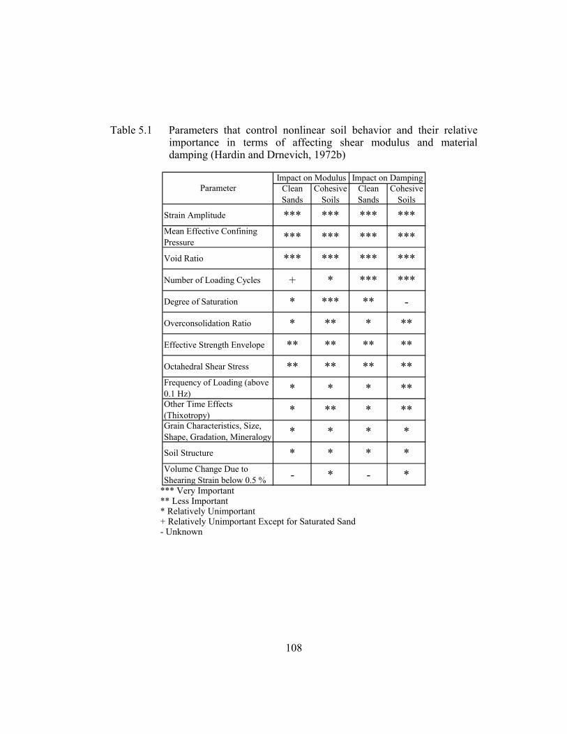
108
Table 5.1 Parameters that control nonlinear soil behavior and their relative importance in terms of affecting shear modulus and material damping (Hardin and Drnevich, 1972b)
Clean Sands
Cohesive Soils
Clean Sands
Cohesive Soils
Strain Amplitude *** *** *** ***Mean Effective Confining Pressure *** *** *** ***
Void Ratio *** *** *** ***
Number of Loading Cycles + * *** ***
Degree of Saturation * *** ** -
Overconsolidation Ratio * ** * **
Effective Strength Envelope ** ** ** **
Octahedral Shear Stress ** ** ** **Frequency of Loading (above 0.1 Hz) * * * **Other Time Effects (Thixotropy) * ** * **Grain Characteristics, Size, Shape, Gradation, Mineralogy * * * *
Soil Structure * * * *Volume Change Due to Shearing Strain below 0.5 % - * - *
Impact on Modulus Impact on DampingParameter
*** Very Important ** Less Important * Relatively Unimportant + Relatively Unimportant Except for Saturated Sand - Unknown

109
Hardin and Drnevich (1972b) also proposed that a hyperbolic relationship
can be used to relate shear stress and shearing strain in modeling dynamic soil
behavior. The Hyperbolic model, illustrated in Figure 5.1a, can be expressed as:
maxmax
1τ
γγτ+
=
G
(5.1)
where: τ = shear stress,
γ = shearing strain,
Gmax = small-strain shear modulus, and
τmax = shear strength of the soil.
In this model, reference strain is defined as:
max
max
Grτ
γ = (5.2)
By dividing both sides of Equation 5.1 by γ, the secant shear modulus, G, is
obtained:
maxmax
11
τγ
+=
G
G (5.3)
The normalized modulus reduction curve can be evaluated from Equation
5.3 by rearranging the equation as follows:
r
GG
γγ
+=
1
1
max
(5.4)
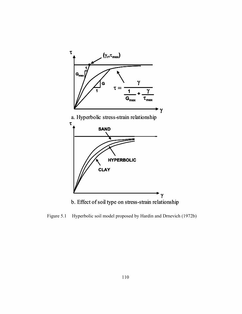
110
1
G
1Gmax
(γr,τmax)τ
γ
τ =γ
1 γGmax τmax
+1
G
1Gmax
(γr,τmax)τ
γ
τ =γ
1 γGmax τmax
+
SAND
CLAY
HYPERBOLIC
τ
γ
SAND
CLAY
HYPERBOLIC
τ
γ
a. Hyperbolic stress-strain relationship
b. Effect of soil type on stress-strain relationship
1
G
1Gmax
(γr,τmax)τ
γ
τ =γ
1 γGmax τmax
+1
G
1Gmax
(γr,τmax)τ
γ
τ =γ
1 γGmax τmax
+
SAND
CLAY
HYPERBOLIC
τ
γ
SAND
CLAY
HYPERBOLIC
τ
γ
a. Hyperbolic stress-strain relationship
b. Effect of soil type on stress-strain relationship
Figure 5.1 Hyperbolic soil model proposed by Hardin and Drnevich (1972b)
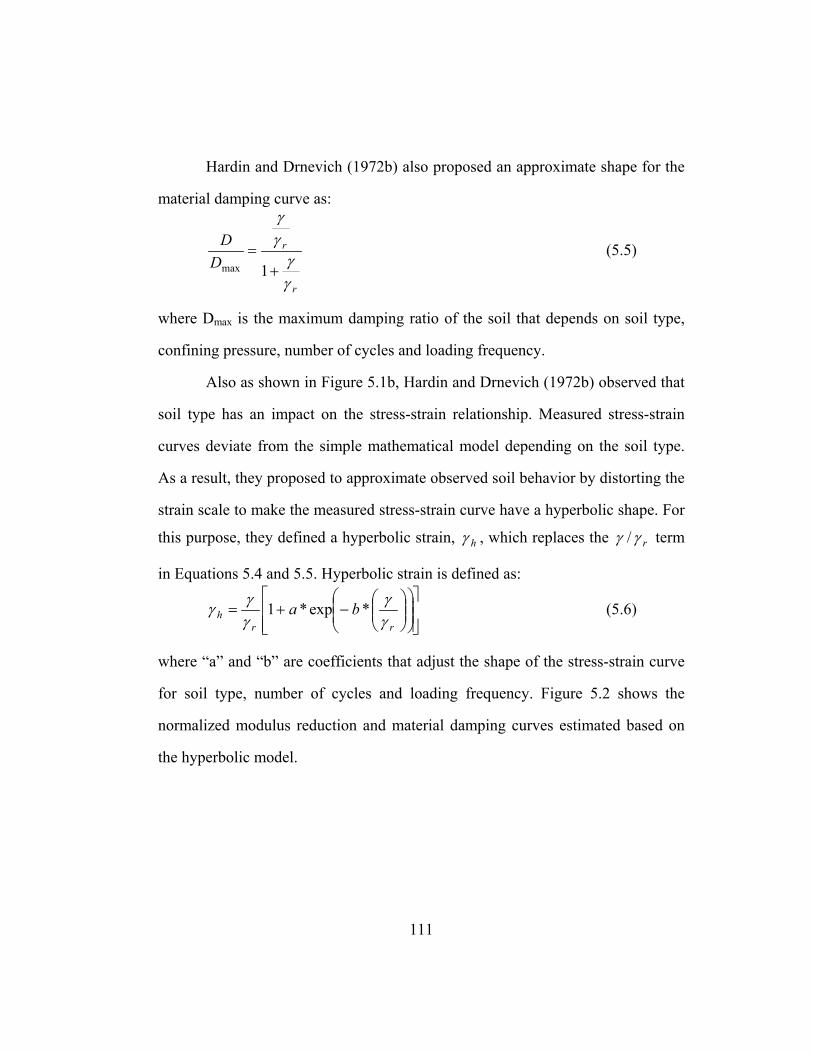
111
Hardin and Drnevich (1972b) also proposed an approximate shape for the
material damping curve as:
r
r
DD
γγ
γγ
+=
1max (5.5)
where Dmax is the maximum damping ratio of the soil that depends on soil type,
confining pressure, number of cycles and loading frequency.
Also as shown in Figure 5.1b, Hardin and Drnevich (1972b) observed that
soil type has an impact on the stress-strain relationship. Measured stress-strain
curves deviate from the simple mathematical model depending on the soil type.
As a result, they proposed to approximate observed soil behavior by distorting the
strain scale to make the measured stress-strain curve have a hyperbolic shape. For
this purpose, they defined a hyperbolic strain, hγ , which replaces the rγγ / term
in Equations 5.4 and 5.5. Hyperbolic strain is defined as:
−+=
rrh ba
γγ
γγγ *exp*1 (5.6)
where “a” and “b” are coefficients that adjust the shape of the stress-strain curve
for soil type, number of cycles and loading frequency. Figure 5.2 shows the
normalized modulus reduction and material damping curves estimated based on
the hyperbolic model.
112
1.0
0.8
0.6
0.4
0.2
0.0
G/Gmax
0.01 0.1 1 10 100Hyperbolic Strain, γh
1.0
0.8
0.6
0.4
0.2
0.0
D/Dmax
G/Gmax = 1 / (1 + γh)D/Dmax = 1 - G/Gmax
Figure 5.2 The normalized modulus reduction and material damping curves estimated based on the hyperbolic model
The empirical equations proposed by Hardin and Drnevich (1972b)
account for the effects of plasticity index, overconsolidation ratio and confining
pressure mainly through adjusting reference strain. Effects of soil type, number of
loading cycles, loading frequency and saturation are taken into consideration by
adjusting Dmax in Equation 5.5 and the “a” and “b” coefficients in Equation 5.6.
Hardin and Drnevich (1972b) proposed graphs and equations based on their
research and experience. The complexity of the procedure in calculating the
normalized modulus reduction and material damping curves limited utilization of
this work in practice. However, their work represented an enormous step forward
in characterizing dynamic soil behavior.
113
5.3 EMPIRICAL RELATIONSHIPS
Numerous other researchers have been influenced by the Hardin and
Drnevich (1972a and b) work and have attempted to refine, improve and
generalize their results. In these other studies, “average” normalized modulus
reduction and material damping curves have been presented. Many of these
curves are widely accepted and utilized in practice. In this section, the strengths
and weaknesses of these empirical curves in estimating nonlinear soil behavior
are discussed.
The effect of mean effective confining pressure on normalized modulus
reduction curves is presented in Figure 5.3 based on resonant column and
torsional shear tests using hollow specimens (Iwasaki et al., 1978). These tests
were performed on saturated clean sand specimens under drained conditions. The
confining pressure used in RCTS testing ranged between 0.25 atm and 2.0 atm.
The results reported in Iwasaki et al. (1978) are consistent with the general trends
outlined in Chapter Four. However, the normalized modulus reduction curves are
found to be somewhat more linear compared to those observed during the course
of this study. The discrepancy is believed to result from the uniform grain size
distribution of the clean sand relative to the natural soils tested as part of this
work.

114
Iwasaki et al. (1978)0.25 atm0.5 atm1.0 atm2.0 atm
0.0001 0.001 0.01 0.1 1Shearing Strain,γ, %
1.2
0.8
0.4
0.0
G/Gmax
Iwasaki et al. (1978)0.25 atm0.5 atm1.0 atm2.0 atm
Iwasaki et al. (1978)0.25 atm0.5 atm1.0 atm2.0 atm
0.0001 0.001 0.01 0.1 1Shearing Strain,γ, %
1.2
0.8
0.4
0.0
G/Gmax
0.0001 0.001 0.01 0.1 1Shearing Strain,γ, %
1.2
0.8
0.4
0.0
G/Gmax
Figure 5.3 The effect of confining pressure on normalized modulus reduction curve for Toyoura Sand (Iwasaki et al., 1978)
Results of cyclic triaxial tests on specimens made of the same saturated
clean sand are presented in Figure 5.4 (Kokusho, 1980). The effect of mean
effective confining pressure (cell pressure) was quantified for material damping
curves as well as for normalized modulus reduction curves by Kokusho (1980).
As in the case of Iwasaki et al. (1978), the range of cell pressures is restricted to
low confining stresses.
Ni (1987) also reported results of tests on clean sands (shown in Figure
5.5) using RCTS equipment at University of Texas at Austin.
The results reported in Iwasaki et al. (1978), Kokusho (1980) and Ni
(1987) are consistent with each other showing that RCTS and cyclic triaxial test
methods yield similar measurements for clean sand specimens. The normalized
modulus reduction and material damping curves are observed to shift to higher
strains and Dmin is observed to decrease with increasing confining pressure
consistent with the general trends outlined in Chapter Four.

115
20
15
10
5
0
D , %
0.0001 0.001 0.01 0.1 1Shearing Strain, γ, %
Kokusho (1980)0.2 atm0.5 atm1.0 atm
(b)
2.0 atm3.0 atm
1.2
0.8
0.4
0.0
G/Gmax
(a)
20
15
10
5
0
D , %
0.0001 0.001 0.01 0.1 1Shearing Strain, γ, %
Kokusho (1980)0.2 atm0.5 atm1.0 atm
(b)
2.0 atm3.0 atm
20
15
10
5
0
D , %
0.0001 0.001 0.01 0.1 1Shearing Strain, γ, %
Kokusho (1980)0.2 atm0.5 atm1.0 atm
(b)
2.0 atm3.0 atm
1.2
0.8
0.4
0.0
G/Gmax
(a)1.2
0.8
0.4
0.0
G/Gmax
(a)
Figure 5.4 The effect of confining pressure on (a) normalized modulus reduction, and (b) material damping curves for Toyoura Sand (Kokusho, 1980)

116
1.2
0.8
0.4
0.0
G/Gmax
(a)
20
15
10
5
0
D , %
0.0001 0.001 0.01 0.1 1Shearing Strain, γ , %
Ni (1987) 0.41 atm 0.82 atm 1.63 atm 3.27 atm
(b)
Figure 5.5 The effect of confining pressure on (a) normalized modulus reduction, and (b) material damping curves for non-plastic soils (Ni, 1987)
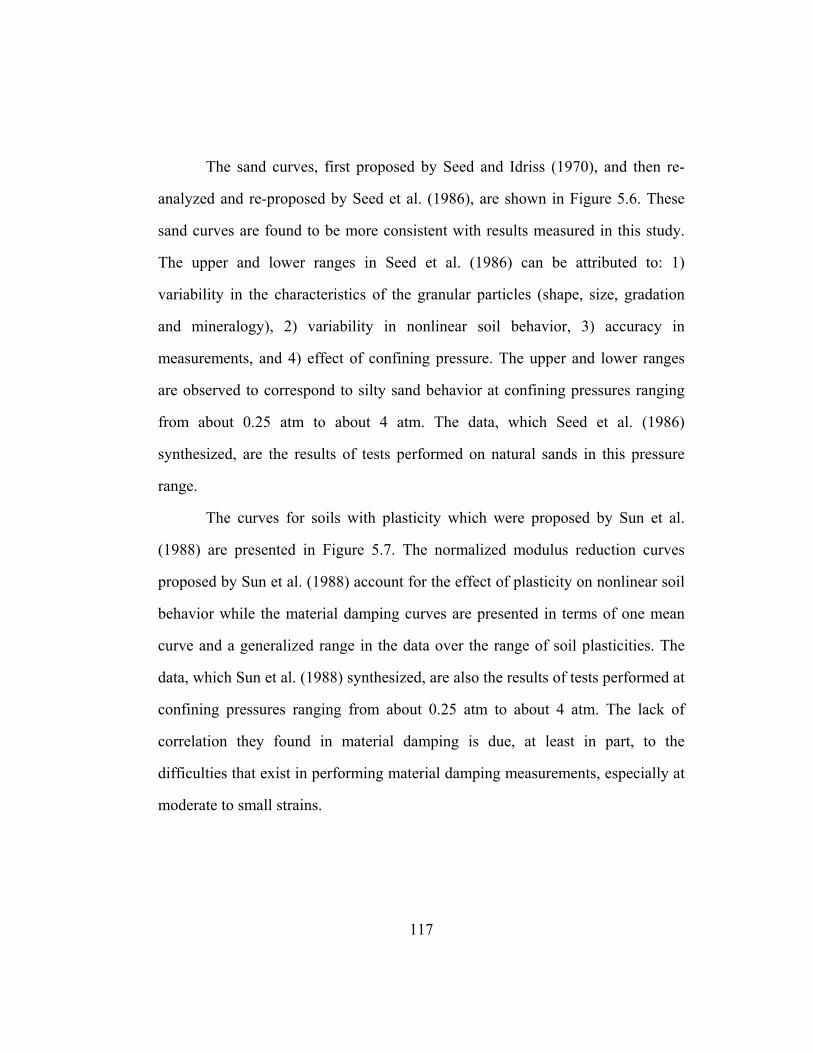
117
The sand curves, first proposed by Seed and Idriss (1970), and then re-
analyzed and re-proposed by Seed et al. (1986), are shown in Figure 5.6. These
sand curves are found to be more consistent with results measured in this study.
The upper and lower ranges in Seed et al. (1986) can be attributed to: 1)
variability in the characteristics of the granular particles (shape, size, gradation
and mineralogy), 2) variability in nonlinear soil behavior, 3) accuracy in
measurements, and 4) effect of confining pressure. The upper and lower ranges
are observed to correspond to silty sand behavior at confining pressures ranging
from about 0.25 atm to about 4 atm. The data, which Seed et al. (1986)
synthesized, are the results of tests performed on natural sands in this pressure
range.
The curves for soils with plasticity which were proposed by Sun et al.
(1988) are presented in Figure 5.7. The normalized modulus reduction curves
proposed by Sun et al. (1988) account for the effect of plasticity on nonlinear soil
behavior while the material damping curves are presented in terms of one mean
curve and a generalized range in the data over the range of soil plasticities. The
data, which Sun et al. (1988) synthesized, are also the results of tests performed at
confining pressures ranging from about 0.25 atm to about 4 atm. The lack of
correlation they found in material damping is due, at least in part, to the
difficulties that exist in performing material damping measurements, especially at
moderate to small strains.

118
1.2
0.8
0.4
0.0
G/Gmax
(a)
20
15
10
5
0
D, %
0.0001 0.001 0.01 0.1 1Shearing Strain, γ , %
Seed et al., (1986)Average for SandsRange
(b)
Figure 5.6 Empirical (a) normalized modulus reduction, and (b) material damping curves proposed by Seed et al. (1986)
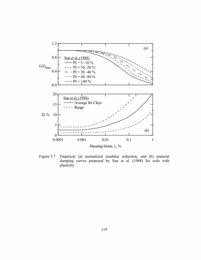
119
1.2
0.8
0.4
0.0
G/Gmax
Sun et al.,(1988)PI = 5 -10 %PI = 10 -20 %PI = 20 -40 %PI = 40 -80 %PI = >80 %
(a)
20
15
10
5
0
D, %
0.0001 0.001 0.01 0.1 1Shearing Strain, γ , %
Sun et al.,(1988)Average for ClaysRange
(b)
Figure 5.7 Empirical (a) normalized modulus reduction, and (b) material damping curves proposed by Sun et al. (1988) for soils with plasticity

120
The curves proposed by Idriss (1990) are presented in Figure 5.8. Two
“average” normalized modulus reduction curves are proposed by Idriss (1990): 1)
for sands and 2) for clays. On the other hand, a single material damping curve is
proposed for all soil types. The normalized modulus reduction curve proposed for
sands is consistent with Seed et al. (1986) while the modulus reduction curve
proposed for clays represents a high (about 50 %) plasticity clay based on the
curves proposed by Vucetic and Dobry (1991) which are discussed below. The
proposed material damping curve is similar to the lower bound curve proposed by
Seed et al. (1986). A unified material damping curve for all soil types can also be
attributed to uncertainty in damping measurements.
The curves proposed by Vucetic and Dobry (1991) are presented in Figure
5.9. The normalized modulus reduction and material damping curves proposed in
their study account for the effect of plasticity on nonlinear soil behavior.
However, the values of small-strain damping, Dmin, have been left somewhat
undefined due to the lack of small-strain data. As shown in Figure 5.9, the value
of Dmin is predicted to decrease with increasing soil plasticity, while the opposite
trend is observed during the course of this study as discussed in Chapter Four.
The data, which Vucetic and Dobry (1991) synthesized, are also the results of
tests performed at confining pressures ranging from about 0.25 atm to about 4
atm.
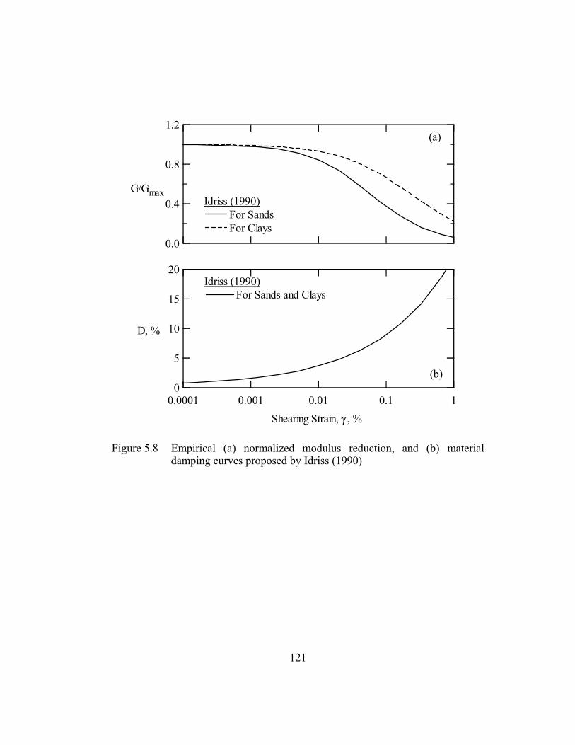
121
1.2
0.8
0.4
0.0
G/GmaxIdriss (1990)
For SandsFor Clays
(a)
20
15
10
5
0
D, %
0.0001 0.001 0.01 0.1 1Shearing Strain, γ , %
Idriss (1990)For Sands and Clays
(b)
Figure 5.8 Empirical (a) normalized modulus reduction, and (b) material damping curves proposed by Idriss (1990)

122
1.2
0.8
0.4
0.0
G/Gmax
(a)
20
15
10
5
0
D, %
0.0001 0.001 0.01 0.1 1Shearing Strain, γ , %
Vucetic and Dobry (1991)Non-PlasticPI = 15 %PI = 30 %PI = 50 %PI = 100 %PI = 200 %
(b)
Figure 5.9 Empirical (a) normalized modulus reduction, and (b) material damping curves proposed by Vucetic and Dobry (1991)

123
The curves proposed by Ishibashi and Zhang (1993) are presented in
Figures 5.10 and 5.11. In their study, a set of equations, which generate
normalized modulus reduction and material damping curves changing with
confining pressure, oσ , and soil plasticity, PI, are proposed. The equations
associated with the normalized modulus reduction curve are: omPIm
oPIKG
G −= ),(
max),( γσγ (5.7)
where:
3.10145.04.0
000556.0lntanh1272.0),( PIo emPIm −
−=−
γγ (5.8)
++=
492.0)(000102.0lntanh15.0),(
γγ PInPIK (5.9)
707015150
0
10*7.210*0.710*37.3
0.0
)(
115.15
976.17
404.16
>≤<≤<
=
=
−
−
−
PIPIPI
PI
PIPIPI
PIn (5.10)
Ishibashi and Zhang (1993) proposed to associate the material damping curve
with the normalized modulus reduction curve as follows:
( )
+
−
+=
−
1547.1586.02
1333.0
max
2
max
0145.0 3.1
GG
GGeD
PI (5.11)

124
1.2
0.8
0.4
0.0
G/Gmax
(a)
20
15
10
5
0
D, %
0.0001 0.001 0.01 0.1 1Shearing Strain, γ , %
Ishibashi and Zhang (1993)
0.25 atm1.00 atm4.00 atm16.0 atm
(b)
Figure 5.10 The effect of confining pressure on (a) normalized modulus reduction, and (b) material damping curves for non-plastic soils (Ishibashi and Zhang, 1993)

125
1.2
0.8
0.4
0.0
G/Gmax
(a)
20
15
10
5
0
D, %
0.0001 0.001 0.01 0.1 1Shearing Strain, γ , %
Ishibashi and Zhang (1993)
Non-PlasticPI = 50 %
(b)
Figure 5.11 Empirical (a) normalized modulus reduction, and (b) material damping curves proposed by Ishibashi and Zhang (1993)

126
The data, which Ishibashi and Zhang (1993) synthesized, are the results of
tests performed at confining pressures less than 10 atm. Unfortunately, the
proposed set of equations are observed to give unrealistic relationships at higher
pressures, as illustrated in Figure 5.10 by the curves at oσ = 16 atm. At high
confining pressures, these equations predict normalized shear modulus values
exceeding 1.0 at intermediate strains. At the same time, negative values of
material damping ratio may be predicted using Equation 5.11 under the same
circumstances.
The equations proposed by Ishibashi and Zhang (1993) are also observed
not to be accurate in representing the general trends related with Dmin. These
equations ignore the effect of confining pressure on Dmin, and the value of Dmin is
predicted to decrease with increasing soil plasticity, while the opposite trend is
presented in Chapter Four.
As part of a research project funded by Electric Power Research Institute,
EPRI, a total of 35 undisturbed soil samples from 5 geotechnical sites (Treasure
Island, Gilroy, Oakland Outer Harbor, San Francisco Airport and Lotung) were
tested in the soil dynamics laboratory using the combined RCTS equipment at
The University of Texas at Austin. These samples were taken from a depth range
of 3 m to 150 m and were tested over a wide range of confining pressures. The
results of these tests are also utilized in this study as discussed in Chapter Three.
The normalized modulus reduction and material damping curves based on the
EPRI (1993c) study are presented in Figures 5.12 and 5.13.

127
Figure 5.12 Variation in empirical (a) normalized modulus reduction, and (b) material damping curves with depth (EPRI, 1993c)
(a)
(b)
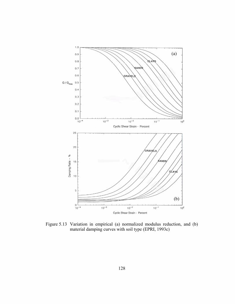
128
Figure 5.13 Variation in empirical (a) normalized modulus reduction, and (b) material damping curves with soil type (EPRI, 1993c)
(a)
(b)

129
In Figure 5.12, the shift in both the normalized modulus reduction and
material damping curves to higher strain levels and the decrease in Dmin with
increasing depth is consistent with the general trends regarding the effect of
confining pressure on nonlinear soil behavior outlined in Chapter Four.
In Figure 5.13, the effect of soil type and plasticity on the normalized
modulus reduction and material damping curves at moderate confining pressures
(at which bulk of the EPRI data is collected) is presented. As discussed in Section
4.9, an increase in Dmin and a simultaneous shift of the material damping curve to
higher strain levels with increasing PI is not shown in any empirical curves except
for the EPRI (1993c) study.
5.4 SUMMARY
The comprehensive study performed by Hardin and Drnevich (1972a and
b) is introduced at the beginning of this chapter in order to familiarize the reader
with the basis of generic curves widely used in the state-of-practice. The generic
curves presently utilized in practice are then discussed. It is important to note that
the generic curves proposed by Seed et al. (1986), Sun et al. (1988), Idriss (1990),
and Vucetic and Dobry (1991) are based on data collected at around 1-atm
confining pressure and these curves do not capture the effect of confining pressure
on nonlinear soil behavior.
Although Iwasaki et al. (1978) and Kokusho (1980) studied the impact of
confining pressure, these studies were limited to observations on clean sands
tested at low pressures.
130
The set of equations proposed by Ishibashi and Zhang (1993) account for
both soil plasticity and confining pressure on nonlinear behavior. However, these
equations are based on data collected at confining pressures less than 10 atm and
are observed to give unrealistic values at higher pressures. Also, the effect of soil
plasticity on Dmin is not represented accurately in any of the generic curves widely
used in the state-of-practice.
The empirical curves from the EPRI (1993c) study are based on data
collected over a relatively wider range of confining pressures and are consistent
with the general trends outlined in Chapter Four. Although the EPRI (1993c)
study is one of the most comprehensive studies of nonlinear soil behavior, the
effects of some of the factors such as loading frequency and number of cycles are
not accounted for as part of this work.
The new empirical curves based on the four-parameter soil model
discussed in Chapter Six are formulated to accurately represent (consistent with
the general trends outlined in Chapter Four) the effects of soil type, confining
pressure, loading frequency and number of cycles on the normalized modulus
reduction and material damping curves. These factors are shown to be the key
factors affecting nonlinear dynamic soil behavior for “competent” soils as
summarized in Table 4.1.

131
CHAPTER 6
PROPOSED SOIL MODEL
6.1 INTRODUCTION
In this chapter, a four-parameter model that can be used to characterize
normalized modulus reduction and material damping curves is proposed. This
model is used to develop empirical curves that are based on the hyperbolic soil
model originally developed by Hardin and Drnevich (1972b). The basic
hyperbolic relationship between stress and strain is slightly modified in order to
accommodate a better fit to the modulus reduction curves measured in the
laboratory.
The equation for the material damping curve is related to the shape of the
modulus reduction curve assuming the validity of Masing behavior (Masing,
1926) combined with two modifying parameters. To start, Masing behavior is
used to calculate material damping by evaluating the hysteresis loops that should
form for a given modulus reduction curve and two-way stress reversals. This
material damping curve is then modified using two parameters to fit the
laboratory data as discussed below.
A parametric study is also presented in this chapter to assist the reader in
becoming familiar with the modified hyperbolic model.

132
6.2 NORMALIZED MODULUS REDUCTION CURVE
The hyperbolic model proposed by Hardin and Drnevich (1972b) and the
modification of the model is discussed in this section. A modified hyperbolic
model is utilized to evaluate and model dynamic soil properties in this study.
As discussed in Chapter Five, a normalized modulus reduction curve
based on the hyperbolic model can be expressed as:
r
GG
γγ
+=
1
1
max
(6.1)
It is easy to see that reference strain, γr, corresponds to the strain amplitude when
shear modulus reduces to one half of Gmax. If one uses this approach in defining
γr, reference strain for any given normalized modulus reduction curve can be
easily evaluated from laboratory measurements as long as G/Gmax values around
0.5 are measured during testing. In fact, γr = γG/Gmax=0.5 is a key characteristic of
the hyperbolic model as employed in this research.
In this study, a relatively simple approach is utilized to fit measured stress-
strain curves. A curvature coefficient, a, is integrated into the normalized modulus
reduction curve (Darendeli, 1997) as follows:
a
r
GG
+
=
γγ1
1
max
(6.2)
The curvature coefficient, as the name implies, has an impact on the curvature of
the normalized modulus reduction curve. The reference strain still corresponds to
the strain amplitude when shear modulus reduces to one half of Gmax. The
advantage of this modification is its simplicity. However, depending on the value

133
of the curvature coefficient, the calculated stress-strain curve may not be
asymptotic to the horizontal line defined by τmax. Since this study is an effort to
model strain amplitudes far below failure, the success of this equation in
modeling soil behavior when full shear strength is mobilized is of lesser concern.
Figure 6.1 shows a normalized modulus reduction curve calculated using
this modification to the Hardin and Drnevich (1972b) hyperbolic model; that is
using Equation 6.2 with γr = γG/Gmax=0.5 = 0.03 % and a = 0.90.
The modified hyperbolic relationship can be used to approximate the
normalized modulus reduction curve of all competent soil types at strains even in
excess of 0.3 % as shown in Chapter Eight.
1.0
0.5
0.0
G/Gmax
0.0001 0.001 0.01 0.1 1Shearing Strain, γ , %
γ r = γG/Gmax=0.5 = 0.03 %
a = 0.90
γ r
Figure 6.1 Normalized modulus reduction curve (of a silty sand at 1 atm effective confining pressure) represented using a modified hyperbolic model

134
6.3 NONLINEAR MATERIAL DAMPING CURVE
Material damping can be assumed to result from at least two separate
phenomena. Part of the energy applied to a soil body is attenuated due to the
friction and/or viscous losses at the contact surfaces between particles. In other
words, regardless of the strain amplitude, some energy loss and, therefore,
equivalent damping should be anticipated. On the other hand, soils are extremely
nonlinear in the strain range of interest (0.0001 % < γ < 1 %) during a design-
level earthquake. The nonlinearity in the stress-strain relationship results in
energy loss in a system. Thus, a second component has to be considered. In this
study, these two sources of damping are handled separately and added to each
other in order to evaluate equivalent damping of soils.
Since material damping resulting from nonlinearity of the stress-strain
relationship is the major component, it is discussed first in this section. As
discussed in Section 6.2, the stress-strain and modulus reduction curves are
directly related to each other for two-way cyclic loading (complete stress
reversals). Once a soil is characterized in terms of its normalized modulus
reduction curve and small-strain shear modulus, it is possible to predict the stress-
strain path that the soil is expected to follow under monotonic loading. Figure
6.2a shows the normalized modulus reduction curve (Figure 6.2a is the same
curve as the one shown in Figure 6.1). This curve is scaled to Gmax = 45 MPa in
Figure 6.2b in order to evaluate the G – log γ relationship. Shear stress can be
expressed as:
γτ *G= (6.3)

135
1.2
0.8
0.4
0.0
G/Gmax
(a)
γ r = 0.03 %a = 0.90
50
40
30
20
10
0
G, MPa
0.0001 0.001 0.01 0.1 1Shearing Strain, γ , %
(b)
0.015
0.010
0.005
0.000
τ,
1.00.80.60.40.20.0Shearing Strain, γ , %
(c)
MPa
Figure 6.2 Stress-strain curve (of a silty sand at 1 atm effective confining pressure) estimated based on a modified reference strain model
136
and the stress-strain curve is easily calculated from the G – log γ relationship. The
resulting stress-strain curve is presented in Figure 6.2c. This curve is theoretically
the stress-strain path under monotonic loading for the material characterized by
the normalized modulus reduction curve in Figure 6.2a and Gmax = 45 MPa.
Masing (1926) assumed that the stress-strain path during cyclic loading
could be related to the monotonic loading stress-strain path, which is also called
the backbone curve. His first attempt to relate these two stress-strain paths is
typically called “Masing behavior”. As presented in Figure 6.3, Masing behavior
assumes that hysteresis loops for two-way cyclic loading can be constructed by
scaling the backbone curve by a factor of two. After initial loading, the scaled
curve is flipped on the horizontal and vertical axes, respectively, and placed at the
end of the backbone curve to represent the unloading path. In order to represent
reloading, the scaled curve is placed at the end of the unloading path. As
unloading and reloading is continued, the same stress-strain path is followed. This
simple approach is powerful in explaining the mechanism that causes energy loss
and the formation of hysteresis loops. However, its direct application in modeling
nonlinear soil behavior is limited and has been shown to perform poorly in
various strain ranges as discussed below.
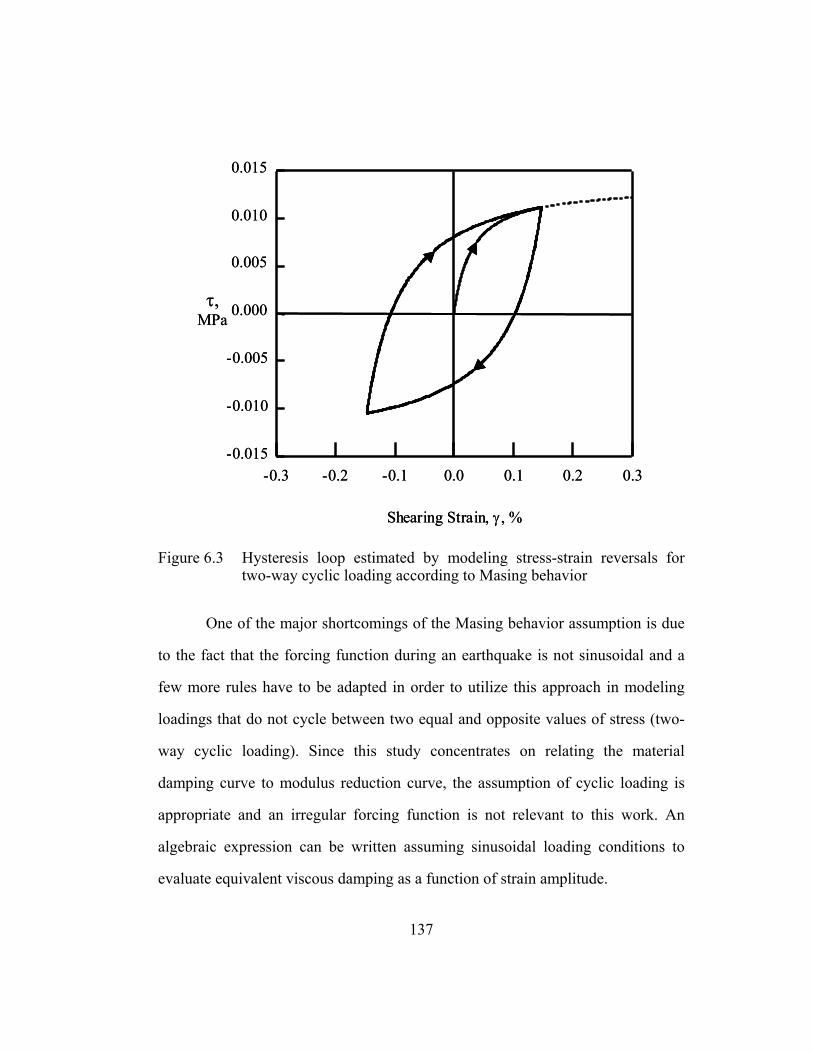
137
-0.015
-0.010
-0.005
0.000
0.005
0.010
0.015
τ,MPa
-0.3 -0.2 -0.1 0.0 0.1 0.2 0.3
Shearing Strain, γ , %
-0.015
-0.010
-0.005
0.000
0.005
0.010
0.015
τ,MPa
-0.3 -0.2 -0.1 0.0 0.1 0.2 0.3
Shearing Strain, γ , %
Figure 6.3 Hysteresis loop estimated by modeling stress-strain reversals for two-way cyclic loading according to Masing behavior
One of the major shortcomings of the Masing behavior assumption is due
to the fact that the forcing function during an earthquake is not sinusoidal and a
few more rules have to be adapted in order to utilize this approach in modeling
loadings that do not cycle between two equal and opposite values of stress (two-
way cyclic loading). Since this study concentrates on relating the material
damping curve to modulus reduction curve, the assumption of cyclic loading is
appropriate and an irregular forcing function is not relevant to this work. An
algebraic expression can be written assuming sinusoidal loading conditions to
evaluate equivalent viscous damping as a function of strain amplitude.

138
As discussed in Section 2.4 and presented in Figure 6.4, damping ratio can
be calculated using the ratio of the dissipated energy to stored strain energy in one
complete cycle of motion. Assuming Masing behavior, the area inside the
hysteresis loop (AL) can be calculated by integrating the stress-strain curve over
one loading cycle.
1GShear
Stress, τ
Shearing Strain, γ
G = τ / γD = AL / (4 π AT)
AL
AT
1GShear
Stress, τ
Shearing Strain, γ
G = τ / γD = AL / (4 π AT)
G = τ / γD = AL / (4 π AT)
AL
AT
Figure 6.4 Calculation of damping ratio utilizing a hysteresis loop
With Equations 6.2 and 6.3, the stress-strain curve can be expressed as:
max*
1
Ga
r
+
=
γγ
γτ (6.4)
The area inside the hysteresis loop can be related to the integral of the stress-strain
curve as follows:
−= ∫ τγγτ
21*8 dAL (6.5)

139
Equivalent viscous damping is expressed as:
T
Leq A
ADΠ
=4
(6.6)
where: Π = pi (= 3.1416),
AT = stored strain energy (τγ/2),
AL = dissipated energy, and
Deq = equivalent viscous damping.
By combining Equations 6.5 and 6.6, Masing-behavior damping can be written as
a function of strain amplitude as follows:
τγ
τγγτ
214
21*8
sinΠ
−
=∫ d
D gMa (6.7)
By substituting Equation 6.4 into Equation in 6.7, Masing-behavior
damping can be rewritten as follows:
a
r
a
r
a
rgMa
d
D
+
+
−
+
Π=
∫
γγ
γγγ
γγ
γγ
γ
1
121
1*4
2
2
sin (6.8)
For a curvature coefficient, “a”, equal to 1.0, Equation 6.8 reduces to:
r
r
r
rrr
agMaD
γγ
γγγ
γγ
γγγγγ
+
+−
+−
Π==
1
121ln
*42
2
0.1,sin (6.9)
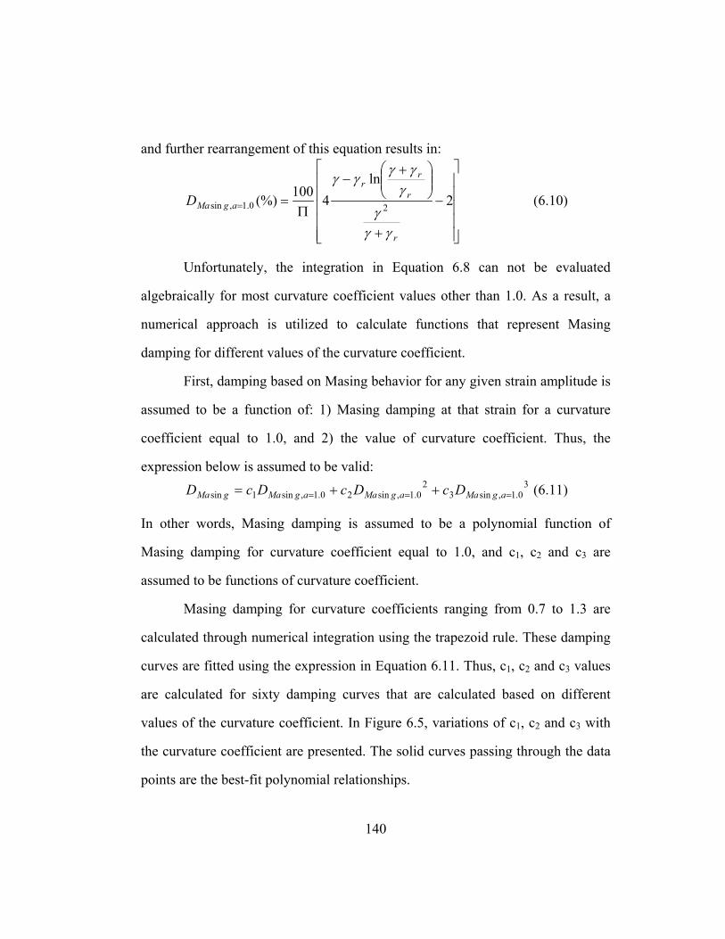
140
and further rearrangement of this equation results in:
−
+
+−
Π== 2
ln4100(%) 20.1,sin
r
r
rr
agMaD
γγγ
γγγ
γγ (6.10)
Unfortunately, the integration in Equation 6.8 can not be evaluated
algebraically for most curvature coefficient values other than 1.0. As a result, a
numerical approach is utilized to calculate functions that represent Masing
damping for different values of the curvature coefficient.
First, damping based on Masing behavior for any given strain amplitude is
assumed to be a function of: 1) Masing damping at that strain for a curvature
coefficient equal to 1.0, and 2) the value of curvature coefficient. Thus, the
expression below is assumed to be valid: 3
0.1,sin32
0.1,sin20.1,sin1sin === ++= agMaagMaagMagMa DcDcDcD (6.11)
In other words, Masing damping is assumed to be a polynomial function of
Masing damping for curvature coefficient equal to 1.0, and c1, c2 and c3 are
assumed to be functions of curvature coefficient.
Masing damping for curvature coefficients ranging from 0.7 to 1.3 are
calculated through numerical integration using the trapezoid rule. These damping
curves are fitted using the expression in Equation 6.11. Thus, c1, c2 and c3 values
are calculated for sixty damping curves that are calculated based on different
values of the curvature coefficient. In Figure 6.5, variations of c1, c2 and c3 with
the curvature coefficient are presented. The solid curves passing through the data
points are the best-fit polynomial relationships.

141
1.1
1.0
0.9
0.8
0.7
c1
(a)
c1 = -1.1143a2 + 1.8618a + 0.2523
R2 = 0.9997
0.04
0.02
0.00
-0.02
c2
(b)
c2 = 0.0805a2 - 0.0710a - 0.0095
R2 = 1.0000
-0.0003
-0.0002
-0.0001
0.0000
0.0001
0.0002
c3
1.31.21.11.00.90.80.7
Curvature Coefficient, a
(c)
c3 = -0.0005a2 + 0.0002a + 0.0003
R2 = 0.9996
Figure 6.5 Variations of c1, c2 and c3 with curvature coefficient, a
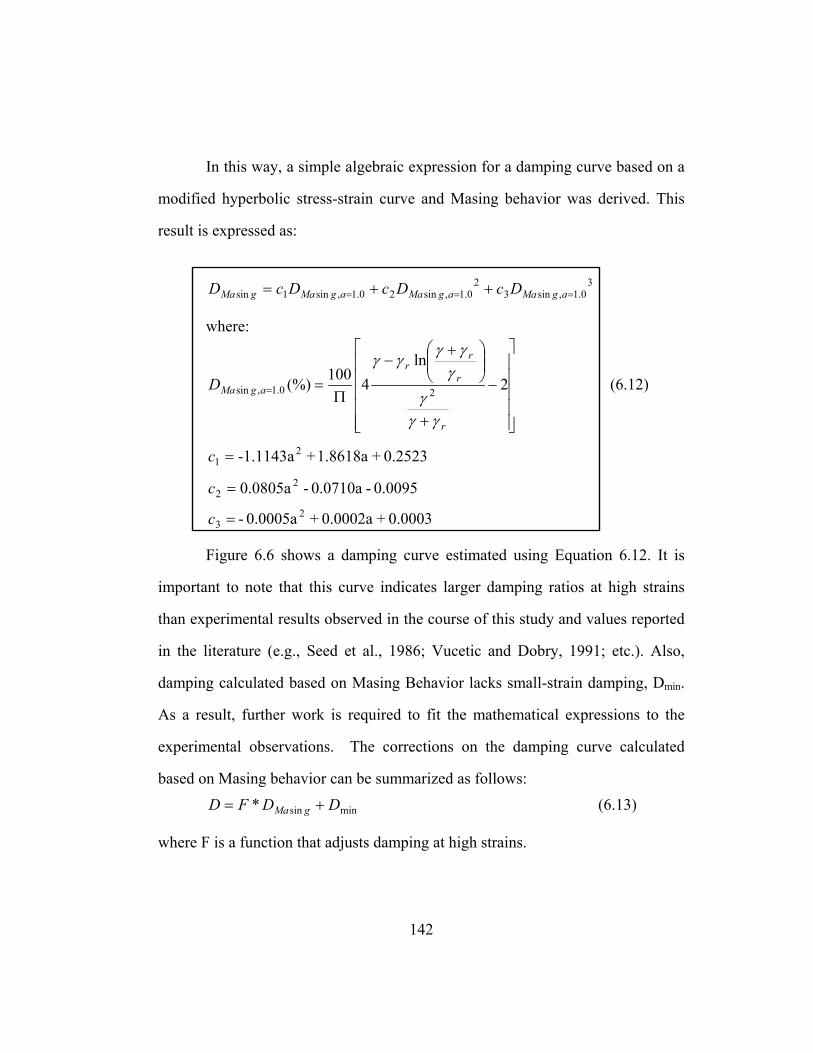
142
In this way, a simple algebraic expression for a damping curve based on a
modified hyperbolic stress-strain curve and Masing behavior was derived. This
result is expressed as:
3
0.1,sin32
0.1,sin20.1,sin1sin === ++= agMaagMaagMagMa DcDcDcD
where:
−
+
+−
Π== 2
ln4100(%) 20.1,sin
r
r
rr
agMaD
γγγ
γγγ
γγ (6.12)
0.2523 + 1.8618a + -1.1143a21 =c
0.0095 - 0.0710a - 0.0805a 22 =c
0.0003 + 0.0002a + 0.0005a- 23 =c
Figure 6.6 shows a damping curve estimated using Equation 6.12. It is
important to note that this curve indicates larger damping ratios at high strains
than experimental results observed in the course of this study and values reported
in the literature (e.g., Seed et al., 1986; Vucetic and Dobry, 1991; etc.). Also,
damping calculated based on Masing Behavior lacks small-strain damping, Dmin.
As a result, further work is required to fit the mathematical expressions to the
experimental observations. The corrections on the damping curve calculated
based on Masing behavior can be summarized as follows:
minsin* DDFD gMa += (6.13)
where F is a function that adjusts damping at high strains.

143
60
40
20
0
D, %
0.0001 0.001 0.01 0.1 1Shearing Strain, γ , %
γ r = 0.03 %a = 0.90
Damping values calculated through numerical intagrationDamping values calculated using polynomial approximation
Figure 6.6 Damping curve estimated based on Masing behavior
Stokoe and Lodde (1978) have shown that small-strain properties are
affected by prior high-amplitude cycling. Gmax tends to decrease slightly and Dmin
tends to increase slightly after high-amplitude cycling as shown in Figure 6.7. The
decrease in Gmax should be expected to result in a considerable decrease in the
nonlinear component of material damping. Also, on various geotechnical
earthquake engineering applications (e.g., Stokoe et al., 1998a), a cap on high-
amplitude damping is required in seismic evaluations of critical structures (in
order to be conservative). As a result, function F in Equation 6.13 is replaced with
a function of G/Gmax in the form of:
p
GGbF
=
max* (6.14)
where b and p are parameters that control the characteristics of this function.

144
Figure 6.7 Effect of high-amplitude cycling on low-amplitude shear modulus and material damping ratio (from Stokoe and Lodde, 1978)
Figure 6.8 shows the variation of this function with shearing strain amplitude for
different values of “p”. Using the value of 0.1 for the “p” parameter was observed
to fit the experimental data. In order to simplify the model, the “p” parameter was
replaced with this constant value. Thus, damping adjusted using function F is
expressed as:
gMaAdjusted DG
GbD sin
1.0
max**
= (6.15)
where: b = scaling coefficient,
G/Gmax = normalized modulus, and
DAdjusted = scaled and capped material damping.

145
1.0
0.8
0.6
0.4
0.2
0.0
F
0.0001 0.001 0.01 0.1 1Shearing Strain, γ , %
F = b * (G/Gmax)p
b = 0.56
p = 0p = 0.1p = 0.25
Figure 6.8 Comparison of the variation in F with shearing strain for different values of p
This function acts as a damping cap at very high strains. At the same time,
within this function, a parameter, which is called the scaling coefficient, is
introduced to the model. The scaling coefficient is, in a sense, the ratio of the
measured damping to the damping value which is estimated from Masing
behavior at intermediate strain amplitudes. Hence, the adjusted damping curve in
Figure 6.9b is estimated.
As discussed earlier in this chapter, small-strain damping is also accounted
for in this model. Dmin is added to the adjusted damping curve and the whole
curve is shifted by this amount as shown in Figure 6.9c. The effect of high-
amplitude cycling on Dmin is ignored in this model due to two reasons: 1) for
design purposes, it is always conservative to underestimate material damping
ratio, and 2) even a 50 % increase in Dmin (as shown in Figure 6.7 at γ = 0.1 %)
has a negligible impact on the material damping values at strain levels produced
during design level shaking.

146
60
40
20
0
D, %
(a)
γ r = 0.03 %a = 0.90
25
20
15
10
5
0
D, %
(b)
F = b * (G/Gmax)0.1
b = 0.56
25
20
15
10
5
0
D, %
0.0001 0.001 0.01 0.1 1Shearing Strain, γ , %
(c)
Masing BehaviorAdjusted CurveShifted Curve
Dmin = 0.90 %
Figure 6.9 (a) Damping curve estimated based on Masing behavior, (b) adjusted curve using the scaling coefficient, and (c) shifted curve using the small-strain material damping ratio
147
6.4 PARAMETRIC STUDY OF THE SOIL MODEL
In this section, a parametric study of the soil model is presented so that the
effect of each parameter on the normalized modulus reduction curve and the
material damping curve can be easily visualized. The ability of this four-
parameter model in representing the trends discussed in Chapter Four is also
discussed herein.
6.4.1 Reference Strain, γr
The effect of reference strain on the normalized modulus reduction, stress-
strain and material damping curves is presented in Figure 6.10. As discussed in
Sections 4.5 and 4.9, increasing confining pressure and increasing soil plasticity
both cause shifts to higher strain levels in the normalized modulus reduction and
material damping curves. This trend is accounted for by adjusting this parameter
as shown in Figure 6.10.
6.4.2 Curvature Coefficient, a
The effect of the curvature coefficient on the normalized modulus
reduction, stress-strain and material damping curves is presented in Figures 6.11
through 6.13. Hardin and Drnevich (1972b) have pointed out a relationship
between the shape of the stress-strain curve and soil type, which can be accounted
for with this parameter as shown in these figures.

148
1.0
0.8
0.6
0.4
0.2
0.0
G/Gmax
0.0001 0.001 0.01 0.1 1Shearing Strain, γ , %
Reference Strain, γ r1.00E-2 %3.00E-2 %1.00E-1 %
(a)
0.03
0.02
0.01
0.00
τ,
1.00.80.60.40.20.0Shearing Strain, γ , %
MPa
(b)
30
20
10
0
D, %
0.0001 0.001 0.01 0.1 1Shearing Strain, γ , %
(c)
Figure 6.10 Effect of reference strain on (a) normalized modulus reduction, (b) stress-strain, and (c) material damping curves

149
1.0
0.8
0.6
0.4
0.2
0.0
G/Gmax
0.0001 0.001 0.01 0.1 1Shearing Strain, γ , %
Curvature Coefficient, a0.81.01.2
γ r
Figure 6.11 Effect of the curvature coefficient on the normalized modulus reduction curve
0.008
0.006
0.004
0.002
0.000
τ,
0.040.030.020.010.00Shearing Strain, γ , %
MPa
(a)
0.03
0.02
0.01
0.00
τ,
1.00.80.60.40.20.0Shearing Strain, γ , %
MPa
(b)
Figure 6.12 Effect of the curvature coefficient on the stress-strain curve (a) at small and intermediate strains, and (b) at high strains
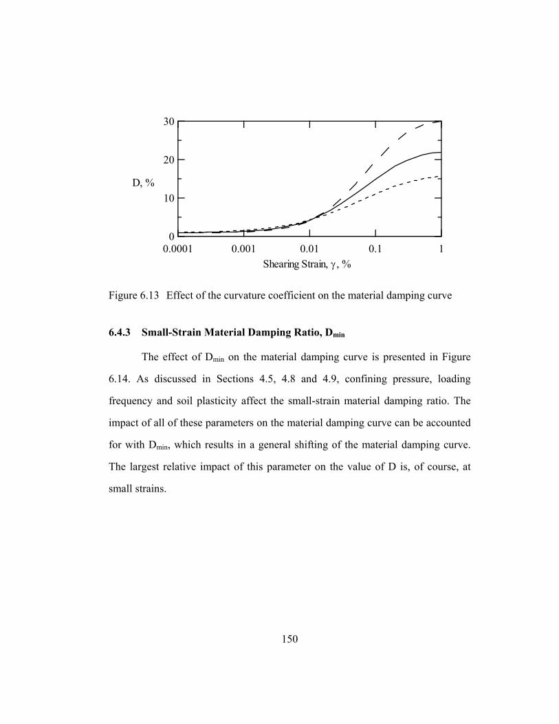
150
30
20
10
0
D, %
0.0001 0.001 0.01 0.1 1Shearing Strain, γ , %
Figure 6.13 Effect of the curvature coefficient on the material damping curve
6.4.3 Small-Strain Material Damping Ratio, Dmin
The effect of Dmin on the material damping curve is presented in Figure
6.14. As discussed in Sections 4.5, 4.8 and 4.9, confining pressure, loading
frequency and soil plasticity affect the small-strain material damping ratio. The
impact of all of these parameters on the material damping curve can be accounted
for with Dmin, which results in a general shifting of the material damping curve.
The largest relative impact of this parameter on the value of D is, of course, at
small strains.

151
30
20
10
0
D, %
0.0001 0.001 0.01 0.1 1Shearing Strain, γ , %
Small Strain Damping, Dmin0.0 %0.9 %3.0 %
Figure 6.14 Effect of Dmin on the material damping curve
6.4.4 Scaling Coefficient, b
The effect of the scaling coefficient on the material damping curve is
presented in Figure 6.15. As discussed in Section 4.7, the number of loading
cycles affects the damping curve, which can be accounted for with this parameter
by varying b with number of cycles.

152
30
20
10
0
D, %
0.0001 0.001 0.01 0.1 1Shearing Strain, γ , %
Scaling Coefficient, b0.400.560.70
Figure 6.15 The effect of scaling coefficient on material damping curve
6.5 SUMMARY
In this chapter, a set of equations based on the Hardin and Drnevich
(1972b) hyperbolic model is proposed to represent the general trends of dynamic
soil properties outlined in Chapter Four.
This empirical model utilizes a modified hyperbolic soil model in order to
represent the stress-strain relationships and, therefore, the normalized modulus
reduction curves. The modified hyperbolic soil model utilizes two parameters
(reference strain and curvature coefficient) and can be expressed as:
a
r
GG
+
=
γγ1
1
max
(6.16)
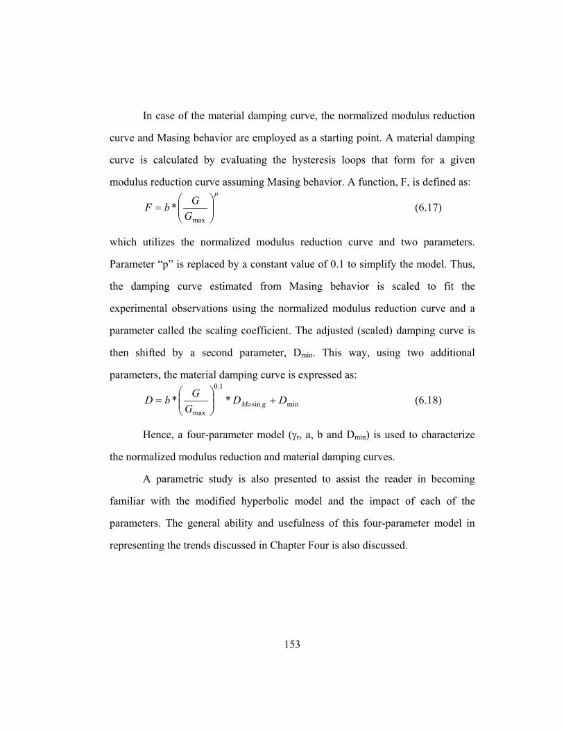
153
In case of the material damping curve, the normalized modulus reduction
curve and Masing behavior are employed as a starting point. A material damping
curve is calculated by evaluating the hysteresis loops that form for a given
modulus reduction curve assuming Masing behavior. A function, F, is defined as: p
GGbF
=
max* (6.17)
which utilizes the normalized modulus reduction curve and two parameters.
Parameter “p” is replaced by a constant value of 0.1 to simplify the model. Thus,
the damping curve estimated from Masing behavior is scaled to fit the
experimental observations using the normalized modulus reduction curve and a
parameter called the scaling coefficient. The adjusted (scaled) damping curve is
then shifted by a second parameter, Dmin. This way, using two additional
parameters, the material damping curve is expressed as:
minsin
1.0
max** DD
GGbD gMa +
= (6.18)
Hence, a four-parameter model (γr, a, b and Dmin) is used to characterize
the normalized modulus reduction and material damping curves.
A parametric study is also presented to assist the reader in becoming
familiar with the modified hyperbolic model and the impact of each of the
parameters. The general ability and usefulness of this four-parameter model in
representing the trends discussed in Chapter Four is also discussed.

154
CHAPTER 7
STATISTICAL ANALYSIS OF COLLECTED DATA USING
FIRST-ORDER, SECOND-MOMENT BAYESIAN METHOD
7.1 INTRODUCTION
In this chapter, the statistical analysis carried out as part of this study is
presented. The statistical tool utilized in this study is briefly explained and the
advantages of using this approach in geotechnical engineering are discussed.
Bayes’ theorem is introduced early in the chapter in order to familiarize
the reader with the concept of systematically utilizing both experience and
observations in statistical analysis. Then, application of the theorem to discrete
and continuous problems is briefly discussed. A discrete example is presented in
order to clarify the methodology. The computational drawbacks in direct
application of Bayes’ theorem are pointed out and an iterative method, which is
used in analyzing the collected data, is presented.
Each parameter of the soil model (presented in Chapter Six) is expressed
in the form of an equation. The equations are formulated so that the impact of
strain amplitude, effective isotropic confining pressure, loading history and
loading frequency on dynamic soil behavior can be properly modeled following
the general trends discussed in Chapter Four. These equations and the form of the
anticipated covariance structure, which describes the deviations between the data
and the model in terms of their magnitude and interrelationships (correlations),
are also presented herein.
155
7.2 BAYESIAN APPROACH
Whenever an engineer faces a problem, he or she attempts to analytically
structure the problem and represent the physical phenomenon by a mathematical
relationship. Once the parameters of the mathematical relationship are
determined, calculations are performed. The solution of the problem is achieved
when the numerical result is expressed as a physical quantity. This method is the
way a structural engineer decides the required reinforcement for a concrete beam
and it is the same method a geotechnical engineer follows to determine the
required pile length for a deep foundation. If the parameters of the mathematical
relationship are estimated accurately, the outcome is a success. The engineer can
develop a safe and economic solution.
In statistical analysis, accurate estimates of parameters require large
amounts of data. In most engineering applications, observed data are limited due
to the fact that data are an expensive commodity. As a result, using judgment and
intuition has always been an essential part of decision making in engineering.
Complex engineering problems require combining information based on
experience with observational data. The Bayesian method is a systematic way of
achieving this goal.
By modeling the unknown parameters as random variables, uncertainty
associated with the estimation of the parameters can be combined with the
inherent variability of the basic random variable through Bayes’ theorem. Thus,
engineering judgment and experience can be incorporated with observed data to
obtain a balanced estimation (Ang and Tang, 1975 and 1990).

156
7.2.1 Bayes’ Theorem
The numerical measure of the likelihood of occurrence of an event, Ei,
relative to all possible outcomes is called the probability of this event, and it is
denoted as P(Ei).
If the probability of an event depends on the occurrence of another event,
the associated probability is called conditional probability. The conditional
probability of E1 assuming E2 has occurred is denoted as P(E1/E2) and it is
expressed as:
)()()/(
2
2121 EP
EEPEEP = (7.1)
where P(E1E2) denotes probability of occurrence of both events.
P(E1E2) can also be expressed in terms of the conditional probability of E2
assuming E1 has occurred using the same form presented in Equation 7.1 as
follows:
)()()/(
1
2112 EP
EEPEEP = (7.2)
By substituting Equation 7.2 into Equation 7.1, the following equation can
be written:
)()(*)/()/(
2
11221 EP
EPEEPEEP = (7.3)
Considering n mutually exclusive and collectively exhaustive events, E1,
E2, …. , En; and another event A in the same sample space, we can write:
∑=
=n
iiEPAPAP
1)(*)()( (7.4)

157
Using the definition of conditional probability, Equation 7.4 can be
expressed as follows.
∑=
=n
iii EPEAPAP
1)(*)/()( (7.5)
Therefore, if the event A has occurred, the probability of occurrence of a
particular event Ei can be expressed by Equation 7.6, which is also known as
Bayes’ theorem, and is expressed as:
∑=
= n
jjj
iii
EPEAP
EPEAPAEP
1)(*)/(
)(*)/()/( (7.6)
7.2.2 Discrete Case
Application of Bayes’ theorem for a discrete problem in order to update an
initial estimate in light of new observations is described in this section.
If a variable X can only take on certain discrete values of x, it is called a
discrete random variable. The outcome of rolling a dice represents such a
variable. It is possible to roll only integer values between 1 and 6. In this case,
the function expressing P(X = x) for all x is utilized to describe the probability
distribution of X. This function is called a probability mass function (PMF).
If a parameter X is often used by an engineer, he or she would have some
prior knowledge of possible values and values more likely to occur than others
based on experience or intuition. This initial information can be represented in
terms of a PMF if X is a discrete random variable. Once additional information
becomes available, the prior assumptions on the parameter are modified or
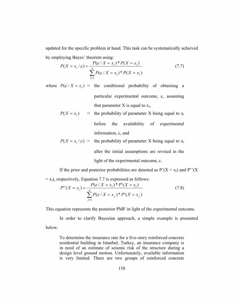
158
updated for the specific problem at hand. This task can be systematically achieved
by employing Bayes’ theorem using:
∑=
==
==== n
iii
iii
xXPxXP
xXPxXPxXP
1)(*)/(
)(*)/()/(
ε
εε (7.7)
where )/( ixXP =ε = the conditional probability of obtaining a
particular experimental outcome, ε, assuming
that parameter X is equal to xi,
)( ixXP = = the probability of parameter X being equal to xi
before the availability of experimental
information, ε, and
)/( εixXP = = the probability of parameter X being equal to xi
after the initial assumptions are revised in the
light of the experimental outcome, ε.
If the prior and posterior probabilities are denoted as P’(X = xi) and P’’(X
= xi), respectively, Equation 7.7 is expressed as follows:
∑=
==
==== n
jjj
iii
xXPxXP
xXPxXPxXP
1)('*)/(
)('*)/()(''
ε
ε (7.8)
This equation represents the posterior PMF in light of the experimental outcome.
In order to clarify Bayesian approach, a simple example is presented
below:
To determine the insurance rate for a five-story reinforced concrete residential building in Istanbul, Turkey, an insurance company is in need of an estimate of seismic risk of the structure during a design level ground motion. Unfortunately, available information is very limited. There are two groups of reinforced concrete
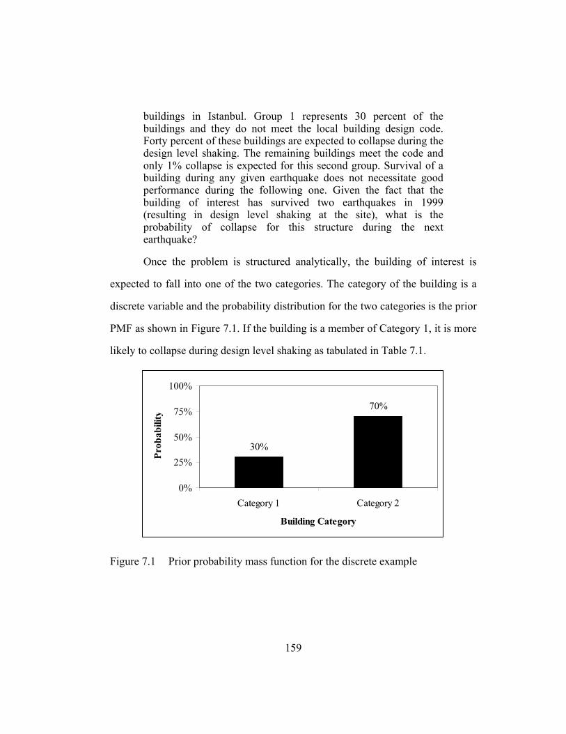
159
buildings in Istanbul. Group 1 represents 30 percent of the buildings and they do not meet the local building design code. Forty percent of these buildings are expected to collapse during the design level shaking. The remaining buildings meet the code and only 1% collapse is expected for this second group. Survival of a building during any given earthquake does not necessitate good performance during the following one. Given the fact that the building of interest has survived two earthquakes in 1999 (resulting in design level shaking at the site), what is the probability of collapse for this structure during the next earthquake?
Once the problem is structured analytically, the building of interest is
expected to fall into one of the two categories. The category of the building is a
discrete variable and the probability distribution for the two categories is the prior
PMF as shown in Figure 7.1. If the building is a member of Category 1, it is more
likely to collapse during design level shaking as tabulated in Table 7.1.
30%
70%
0%
25%
50%
75%
100%
Category 1 Category 2
Building Category
Prob
abili
ty
Figure 7.1 Prior probability mass function for the discrete example

160
Table 7.1 Prior information provided in the discrete example
P’(Category = 1) 30 %P’(Category = 2) 70 %P(collapse / Category = 1) 40 %P(collapse / Category = 2) 1 %
Based on this information, the probability of collapse for a particular
building (not knowing whether or not it was built following the code) can be
calculated as follows:
p’(collapse) = 0.30 * 0.40 + 0.70 * 0.01 (7.9a)
p’(collapse) = 12.7 % (7.9b)
The statement regarding survival of the building during two earthquakes in 1999
is observational data. Assuming survival of the building at two instances are
statistically independent:
P(success) = 1 – P(collapse) (7.10)
P(success 2 consecutive earthquakes) = P(success)2 (7.11)
Based on Equation 7.11, the prior PMF can be updated using Equation 7.12 based
on Bayes’ theorem as:
∑=
==
==== 2
1)i Category ('*)i Category /(
)1 Category ('*)1 Category /()1 Category (''
iPP
PPPε
ε (7.12a)
∑=
==
==== 2
1)i Category ('*)i Category /(
)2 Category ('*)2 Category /()2 Category (''
iPP
PPPε
ε (7.12b)
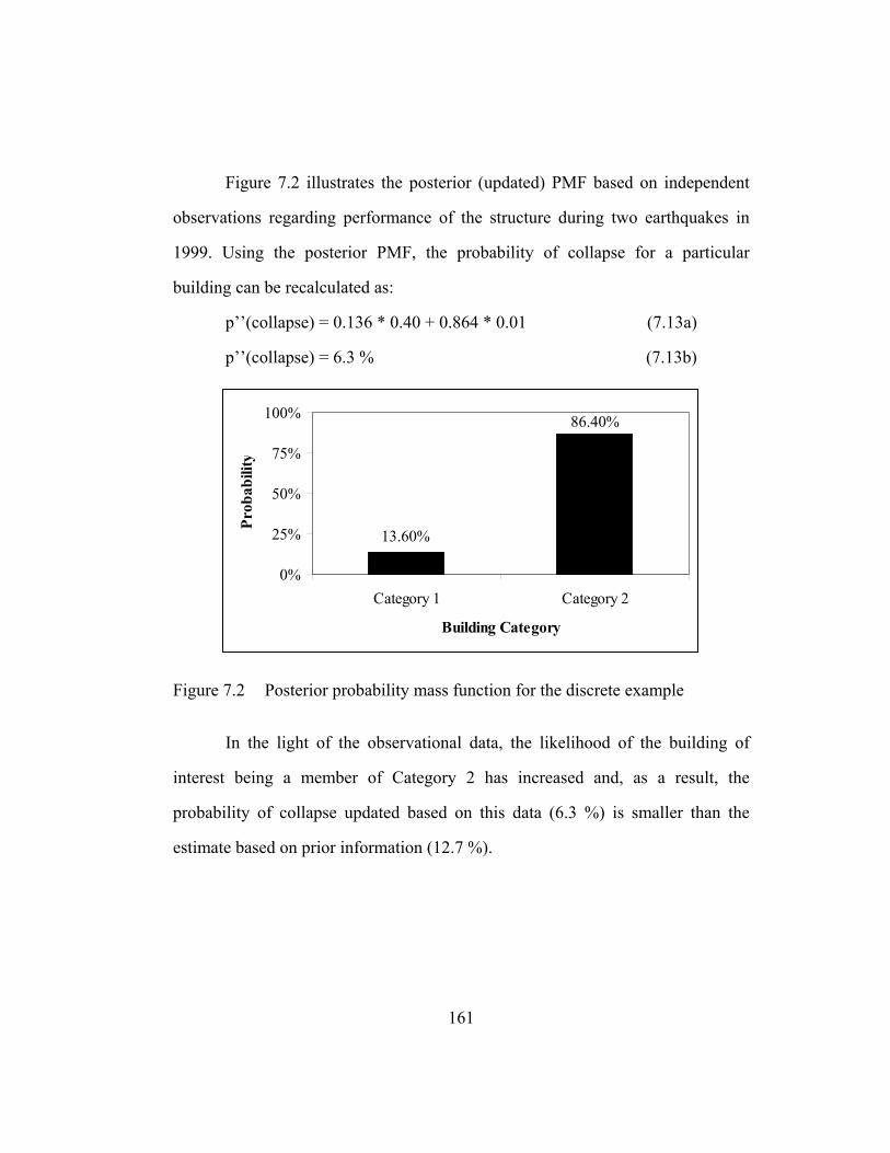
161
Figure 7.2 illustrates the posterior (updated) PMF based on independent
observations regarding performance of the structure during two earthquakes in
1999. Using the posterior PMF, the probability of collapse for a particular
building can be recalculated as:
p’’(collapse) = 0.136 * 0.40 + 0.864 * 0.01 (7.13a)
p’’(collapse) = 6.3 % (7.13b)
13.60%
86.40%
0%
25%
50%
75%
100%
Category 1 Category 2
Building Category
Prob
abili
ty
Figure 7.2 Posterior probability mass function for the discrete example
In the light of the observational data, the likelihood of the building of
interest being a member of Category 2 has increased and, as a result, the
probability of collapse updated based on this data (6.3 %) is smaller than the
estimate based on prior information (12.7 %).

162
7.2.3 Continuous Case
In most cases, the variable of interest does not take on certain discrete
values. Instead, it can take on any value within a continuum. These kinds of
parameters are called continuous random variables. The unit weight of a soil
represents such a variable. In this case, probabilities are associated with intervals.
In other words, the probability of X taking a value between x1 and x2 is relevant.
Thus, a probability density function (PDF) is defined for continuous random
variables. If fx(x) is the PDF of X, the probability of X taking a value between x1
and x2 is:
∫=≤<2
1
)()( 21
x
xx dxxfxXxP (7.14)
In other words,
dxxfdxxXxP x )()( =+≤< (7.15)
Bayes’ theorem can be employed in the same fashion for the continuous
case as in the discrete case as follows:
∫∞
∞−
=
θθθε
θθεθdfP
fPf)(')/(
)(')/()('' (7.16)
where )/( θεP is the conditional probability of obtaining a particular
experimental outcome, ε, assuming that the parameter of interest is equal to θ.
Since )/( θεP is a function of θ it is also called the likelihood function of θ and is
denoted as L(θ). Noting that the denominator in Equation 7.16 is independent of
θ, )('' θf can also be expressed as:
)(')()('' θθθ fkLf = (7.17)
163
where k is a normalizing constant scaling )('' θf to become a proper PDF and
L(θ) is the likelihood of observing the experimental outcome ε assuming a given
value, θ.
In most engineering problems, more than one parameter needs to be
characterized. Even in the simplest case of a linear fit, two parameters are needed,
the intercept and slope. As a result, Equation 7.16 always becomes a bit more
complicated because the denominator has to be integrated for each parameter as
follows:
∫∫∞
∞−
∞
∞−
=
nddfP
fPfφφφφε
φφεφ.....)(')/(......
)(')/()(''
1
rrr
rrrr (7.18)
where a vector of model parameters, φr
, needs to be updated based on a number
of observations.
The integration in Equation 7.18 may become extremely troublesome,
especially when a nonlinear model is being calibrated. The moments of the
updated distribution may also become impossible to compute analytically.
Although the Bayesian approach is a powerful tool, the lack of an analytical
solution makes direct application of the Bayesian approach impractical for most
engineering applications, specifically in those cases dealing with nonlinear
problems.
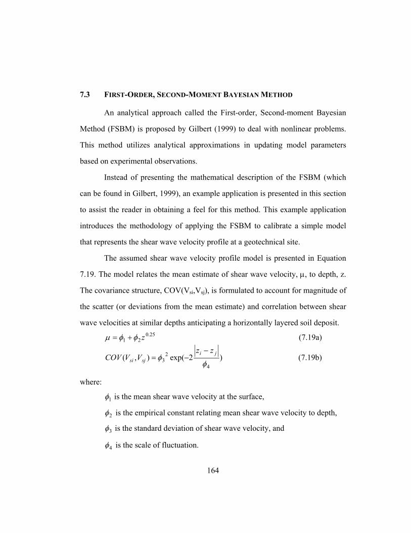
164
7.3 FIRST-ORDER, SECOND-MOMENT BAYESIAN METHOD
An analytical approach called the First-order, Second-moment Bayesian
Method (FSBM) is proposed by Gilbert (1999) to deal with nonlinear problems.
This method utilizes analytical approximations in updating model parameters
based on experimental observations.
Instead of presenting the mathematical description of the FSBM (which
can be found in Gilbert, 1999), an example application is presented in this section
to assist the reader in obtaining a feel for this method. This example application
introduces the methodology of applying the FSBM to calibrate a simple model
that represents the shear wave velocity profile at a geotechnical site.
The assumed shear wave velocity profile model is presented in Equation
7.19. The model relates the mean estimate of shear wave velocity, µ, to depth, z.
The covariance structure, COV(Vsi,Vsj), is formulated to account for magnitude of
the scatter (or deviations from the mean estimate) and correlation between shear
wave velocities at similar depths anticipating a horizontally layered soil deposit. 25.0
21 zφφµ += (7.19a)
)2exp(),(4
23 φ
φ jisjsi
zzVVCOV
−−= (7.19b)
where:
1φ is the mean shear wave velocity at the surface,
2φ is the empirical constant relating mean shear wave velocity to depth,
3φ is the standard deviation of shear wave velocity, and
4φ is the scale of fluctuation.
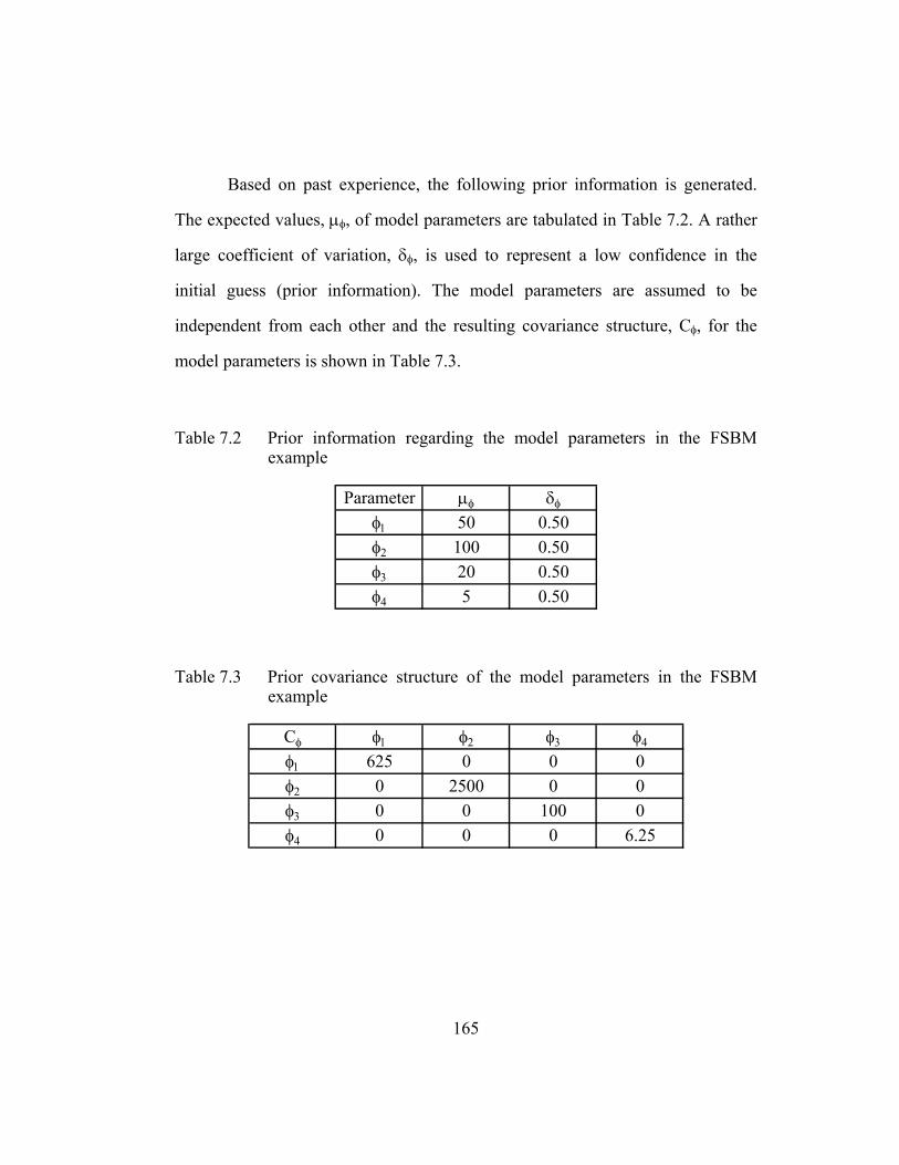
165
Based on past experience, the following prior information is generated.
The expected values, µφ, of model parameters are tabulated in Table 7.2. A rather
large coefficient of variation, δφ, is used to represent a low confidence in the
initial guess (prior information). The model parameters are assumed to be
independent from each other and the resulting covariance structure, Cφ, for the
model parameters is shown in Table 7.3.
Table 7.2 Prior information regarding the model parameters in the FSBM example
Parameter µφ δφ
φ1 50 0.50φ2 100 0.50φ3 20 0.50φ4 5 0.50
Table 7.3 Prior covariance structure of the model parameters in the FSBM example
Cφ φ1 φ2 φ3 φ4
φ1 625 0 0 0φ2 0 2500 0 0φ3 0 0 100 0φ4 0 0 0 6.25

166
The covariance structure within the model should not be confused with the
covariance structure of the model parameters. The covariance structure within the
model expresses the discrepancy between the shear wave velocity profile and the
mathematical representation (model), and it also acknowledges the
interrelationship between shear wave velocities at similar depths and therefore the
interrelationship between closely spaced measurements (in terms of depth). Most
soil deposits are horizontally layered systems and soils sampled from similar
depths are likely to be taken from the same layer resulting in the engineering
properties of these samples to be similar. On the other hand, the covariance
structure of the model parameters describes the uncertainty associated with the
model parameters and how they are related to each other.
The shear wave velocity profile model discussed above is calibrated using
the data presented in Table 7.4 collected at the geotechnical site of interest using
an in-situ seismic method.
Table 7.4 Data used to calibrate the model parameters in the FSBM example
1 1.0 125
2 5.0 1503 5.5 1604 10.0 200
Measurement Depth (m)
Shear Wave Velocity (m/s)
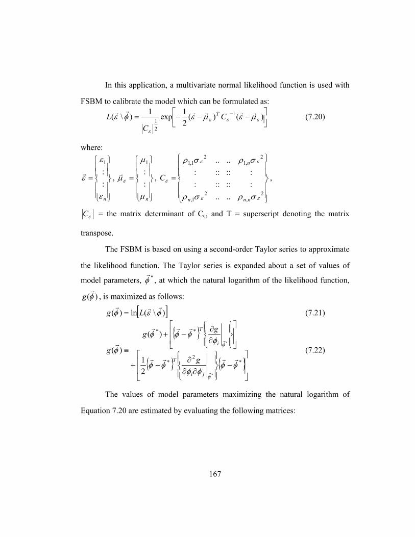
167
In this application, a multivariate normal likelihood function is used with
FSBM to calibrate the model which can be formulated as:
−−−= − )()(
21exp1)\( 1
21 εεε
ε
µεµεφε rrrrrr CC
L T (7.20)
where:
=
nε
ε
ε::1
r ,
=
nµ
µ
µε ::1
r ,
=
2,
21,
2,1
21,1
....::::::::::::
....
εε
εε
ε
σρσρ
σρσρ
nnn
n
C ,
εC = the matrix determinant of Cε, and T = superscript denoting the matrix
transpose.
The FSBM is based on using a second-order Taylor series to approximate
the likelihood function. The Taylor series is expanded about a set of values of
model parameters, *φr
, at which the natural logarithm of the likelihood function,
)(φr
g , is maximized as follows:
[ ])\(ln)( φεφrrr
Lg = (7.21)
{ }
{ } { }
−
∂∂∂
−+
∂∂
−+
≡*
2*
**
*
*
21
)(
)(
φφφφ
φφ
φφφφ
φ
φ
φ
rrrr
rrr
r
r
r
ji
T
i
T
g
gg
g (7.22)
The values of model parameters maximizing the natural logarithm of
Equation 7.20 are estimated by evaluating the following matrices:
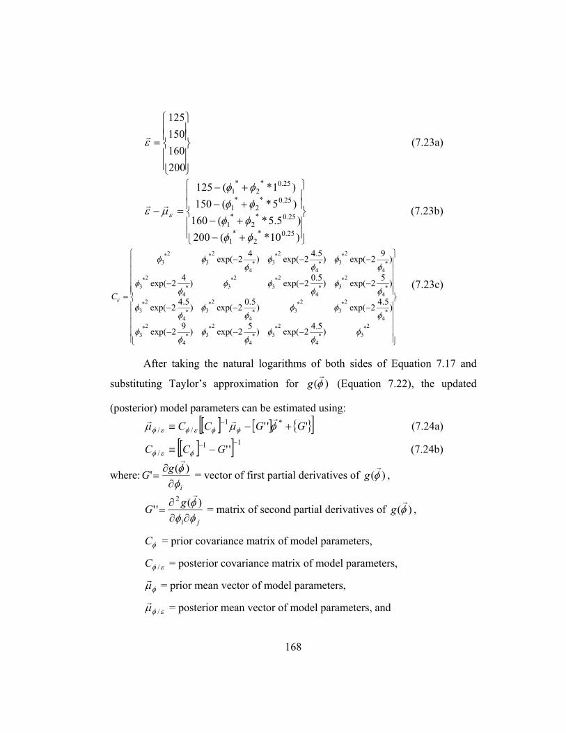
168
=
200160150125
εr (7.23a)
+−+−+−+−
=−
)10*(200)5.5*(160
)5*(150)1*(125
25.0*2
*1
25.0*2
*1
25.0*2
*1
25.0*2
*1
φφφφφφφφ
µε εrr
(7.23b)
−−−
−−−
−−−
−−−
=
2*3*
4
2*3*
4
2*3*
4
2*3
*4
2*3
2*3*
4
2*3*
4
2*3
*4
2*3*
4
2*3
2*3*
4
2*3
*4
2*3*
4
2*3*
4
2*3
2*3
)5.42exp()52exp()92exp(
)5.42exp()5.02exp()5.42exp(
)52exp()5.02exp()42exp(
)92exp()5.42exp()42exp(
φφ
φφ
φφ
φ
φφφ
φφ
φφ
φφ
φφφ
φφ
φφ
φφ
φφφ
εC (7.23c)
After taking the natural logarithms of both sides of Equation 7.17 and
substituting Taylor’s approximation for )(φr
g (Equation 7.22), the updated
(posterior) model parameters can be estimated using: [ ] [ ] { }[ ]''' *1
// GGCC +−≡ − φµµ φφεφεφ
rrr (7.24a)
[ ][ ] 11/ ''
−− −≡ GCC φεφ (7.24b)
where:i
gGφφ
∂∂
=)('r
= vector of first partial derivatives of )(φr
g ,
ji
gGφφφ
∂∂∂
=)(''
2 r
= matrix of second partial derivatives of )(φr
g ,
φC = prior covariance matrix of model parameters,
εφ /C = posterior covariance matrix of model parameters,
φµr = prior mean vector of model parameters,
εφµ /r = posterior mean vector of model parameters, and
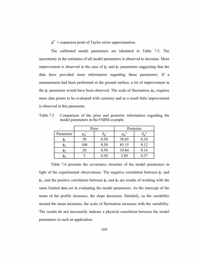
169
*φr
= expansion point of Taylor series approximation.
The calibrated model parameters are tabulated in Table 7.5. The
uncertainty in the estimates of all model parameters is observed to decrease. More
improvement is observed in the case of φ2 and φ3 parameters suggesting that the
data have provided more information regarding these parameters. If a
measurement had been performed at the ground surface, a lot of improvement in
the φ1 parameter would have been observed. The scale of fluctuation, φ4, requires
more data points to be evaluated with certainty and as a result little improvement
is observed in this parameter.
Table 7.5 Comparison of the prior and posterior information regarding the model parameters in the FSBM example
Parameter µφ' δφ' µφ'' δφ''φ1 50 0.50 38.05 0.34φ2 100 0.50 85.15 0.12φ3 20 0.50 10.84 0.16φ4 5 0.50 3.89 0.37
Prior Posterior
Table 7.6 presents the covariance structure of the model parameters in
light of the experimental observations. The negative correlation between φ1 and
φ2, and the positive correlation between φ3 and φ4 are results of working with the
same limited data set in evaluating the model parameters. As the intercept of the
mean of the profile increases, the slope decreases. Similarly, as the variability
around the mean increases, the scale of fluctuation increases with the variability.
The results do not necessarily indicate a physical correlation between the model
parameters in such an application.
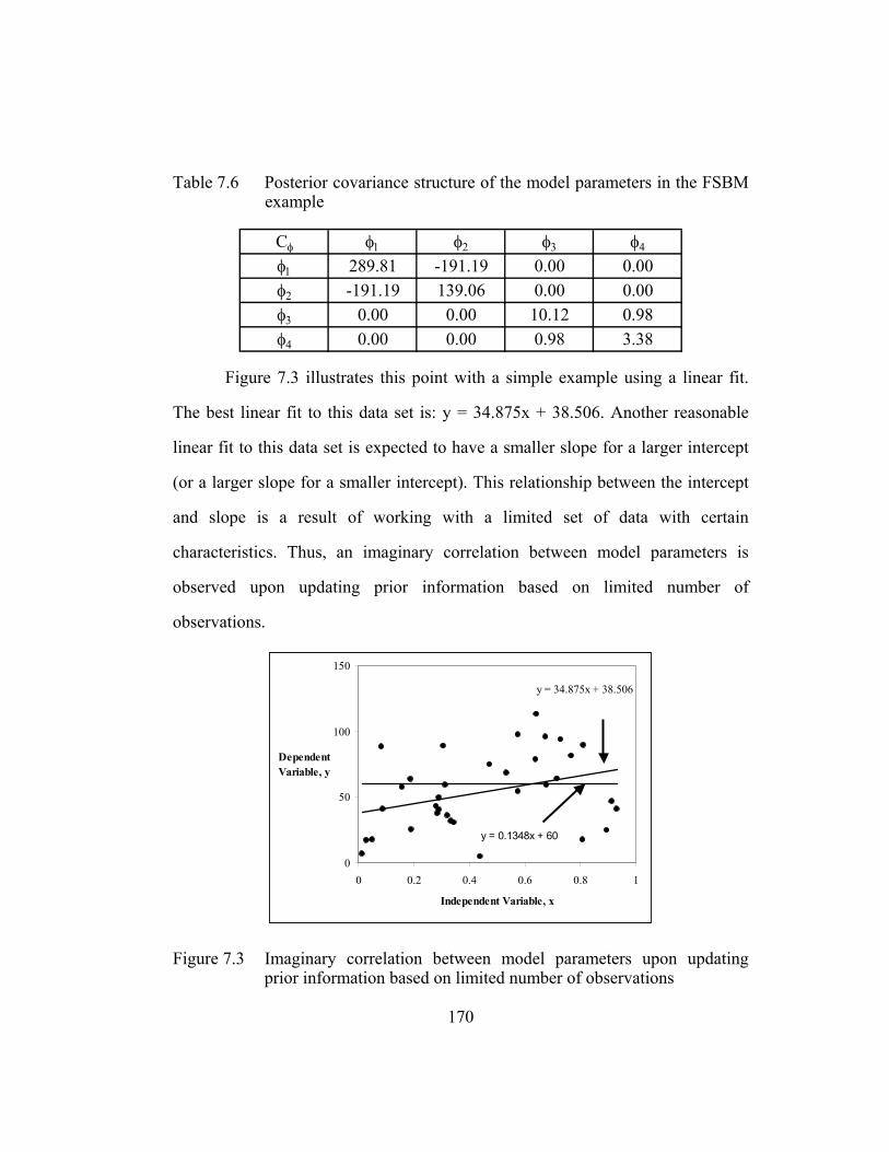
170
Table 7.6 Posterior covariance structure of the model parameters in the FSBM example
Cφ φ1 φ2 φ3 φ4
φ1 289.81 -191.19 0.00 0.00φ2 -191.19 139.06 0.00 0.00φ3 0.00 0.00 10.12 0.98φ4 0.00 0.00 0.98 3.38
Figure 7.3 illustrates this point with a simple example using a linear fit.
The best linear fit to this data set is: y = 34.875x + 38.506. Another reasonable
linear fit to this data set is expected to have a smaller slope for a larger intercept
(or a larger slope for a smaller intercept). This relationship between the intercept
and slope is a result of working with a limited set of data with certain
characteristics. Thus, an imaginary correlation between model parameters is
observed upon updating prior information based on limited number of
observations.
y = 0.1348x + 60
y = 34.875x + 38.506
0
50
100
150
0 0.2 0.4 0.6 0.8 1
Independent Variable, x
Dependent Variable, y
Figure 7.3 Imaginary correlation between model parameters upon updating prior information based on limited number of observations

171
Table 7.7 tabulates the estimates of shear wave velocity at a depth of 10 m
using prior and posterior model parameters. The uncertainties associated with
these estimates are also presented in this table. Upon calibration of the model with
field observations, a tremendous reduction in the uncertainty regarding model
parameters takes place. As a result, the standard deviation associated with the
estimate of shear wave velocity at a depth of 10 m decreases significantly from 95
m/s to 13 m/s. An experienced engineer familiar with the geotechnical site of
interest might have a better idea about the model parameters prior to in-situ
testing and, under such circumstances, the reduction in uncertainty would not be
as significant.
Table 7.7 Posterior covariance structure of the model parameters in the FSBM example
Prior PosteriorExpected Value of Vs at 10 m 227.83 189.47
Variance of Vs at 10 m 9030.69 177.09Standard Deviation of Vs at 10 m 95.03 13.31Variance from Model Uncertainty 8630.69 59.68Variance from Random Variability 400.00 117.41Contribution of Model Uncertainty 0.96 0.34Contribution of Random Variability 0.04 0.66
172
7.4 FORM OF PROPOSED EQUATIONS
A four-parameter (reference strain, curvature coefficient, scaling
coefficient and small-strain material damping ratio) soil model was presented in
Chapter Six. In Chapter Four, the impact of soil type and loading conditions on
nonlinear soil behavior were discussed.
In this section, the problem of accounting for the impact of soil type and
loading conditions on nonlinear soil behavior is structured analytically. The
parameters of the soil model are related to soil plasticity, void ratio, confining
pressure, overconsolidation ratio, loading frequency and number of loading
cycles. The parameters (denoted as φi in these equations) need to be calibrated
based on the experimental observations (resonant column and torsional shear test
results). The resulting equations can then be utilized to estimate the mean
normalized modulus reduction and material damping curves for a given soil type
and loading conditions.
In an effort to represent the trends regarding the scatter of the data, a
second set of equations for standard deviation are proposed in this section. The
modeled correlation structure of the data is also presented herein.
7.4.1 Equations for Mean
Equations used in representing the impact of soil type and loading
conditions on nonlinear soil behavior are described in this section. Proposed
forms of these equations are based on the trends reported in the literature and
experimental observations in the course of this study.

173
As discussed in Section 5.2, the hyperbolic soil model originally proposed
by Hardin and Drnevich (1972b) is slightly modified and this modified
relationship is utilized to represent a normalized modulus reduction curve as:
a
r
GG
+
=
γγ1
1
max
(7.25)
where: G/Gmax = normalized modulus,
γ = shearing strain,
γr = reference strain, and
a = curvature coefficient.
The two parameters in this model (γr and a) can be related to soil type and
loading conditions (σo’ and OCR) as follows: 43 '*)**( 21
φφ σφφγ or OCRPI+= (7.26a)
5φ=a (7.26b)
where: σo’ = mean effective confining pressure (atm),
PI = soil plasticity (%),
OCR = overconsolidation ratio, and
φ1 through φ5 = parameters that relate the normalized modulus reduction
curve to soil type and loading conditions.
These equations can model the shifting of the normalized modulus
reduction curve with increasing soil plasticity, overconsolidation and confining
pressure. When subsets of the data are evaluated, the sensitivity of the curvature
coefficient to soil type and loading conditions can also be studied.
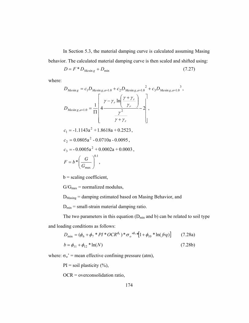
174
In Section 5.3, the material damping curve is calculated assuming Masing
behavior. The calculated material damping curve is then scaled and shifted using:
minsin* DDFD gMa += (7.27)
where: 3
0.1,sin32
0.1,sin20.1,sin1sin === ++= agMaagMaagMagMa DcDcDcD ,
−
+
+−
Π== 2
ln41
20.1,sin
r
r
rr
agMaD
γγγ
γγγ
γγ,
0.2523 + 1.8618a + -1.1143a21 =c ,
0.0095 - 0.0710a - 0.0805a 22 =c ,
0.0003 + 0.0002a + 0.0005a- 23 =c ,
1.0
max*
=
GGbF ,
b = scaling coefficient,
G/Gmax = normalized modulus,
DMasing = damping estimated based on Masing Behavior, and
Dmin = small-strain material damping ratio.
The two parameters in this equation (Dmin and b) can be related to soil type
and loading conditions as follows:
[ ])ln(*1*'*)**( 1076min98 frqOCRPID o φσφφ φφ ++= (7.28a)
)ln(*1211 Nb φφ += (7.28b)
where: σo’ = mean effective confining pressure (atm),
PI = soil plasticity (%),
OCR = overconsolidation ratio,

175
frq = loading frequency,
N = number of loading cycles, and
φ6 through φ12 = parameters that relate material damping curve to soil type
and loading conditions.
Since the material damping curve is directly related to the normalized
modulus reduction curve, any shift in the normalized modulus reduction curve
(due to increasing soil plasticity, overconsolidation and confining pressure) is also
captured in the material damping curve. Small-strain trends in material damping
(discussed in Chapter Four) are accounted for by modeling Dmin separately as a
function of soil plasticity, overconsolidation, confining pressure and loading
frequency. Finally, the impact of number of loading cycles on the material
damping curve is captured in the equation for scaling coefficient.
7.4.2 Equations for Standard Deviation and Covariance Structure
Scatter of the data around the mean estimate is modeled considering the
characteristics of the normalized modulus reduction and material damping curves.
In the case of the normalized modulus reduction curve, less scatter around
the mean is expected at small strains (at which G/Gmax is about 1.0) and at rather
large strains (at which G/Gmax is less than 20%). Uncertainty maximizes around
the reference strain (at which G/Gmax is equal to 0.5). To capture these
characteristics, the standard deviation for a given normalized modulus reduction
curve is modeled as:
)exp()5.0/(
)exp(25.0)exp(
14
2max
1413 φφ
φσ−
−+=GG
NG (7.29)
where: σNG = standard deviation for normalized modulus reduction curve,

176
G/Gmax = estimated normalized shear modulus, and
φ13 and φ14 = parameters that relate standard deviation to mean estimate of
normalized shear modulus.
Figure 7.4 shows the variation of standard deviation with normalized shear
modulus predicted with Equation 7.29. This equation predicts smaller values of
standard deviation for G/Gmax values close to 1.0 and to 0.0. The scatter relative to
an estimated normalized modulus reduction curve is presented in Figure 7.5. This
scatter pattern looks a lot like the lower bound and upper bound curves proposed
by Seed et al. (1986) for sands shown in Figure 4.22.
0.5
0.4
0.3
0.2
0.1
0.0
σNG
1.00.80.60.40.20.0G/Gmax
Figure 7.4 Variation of standard deviation with normalized shear modulus
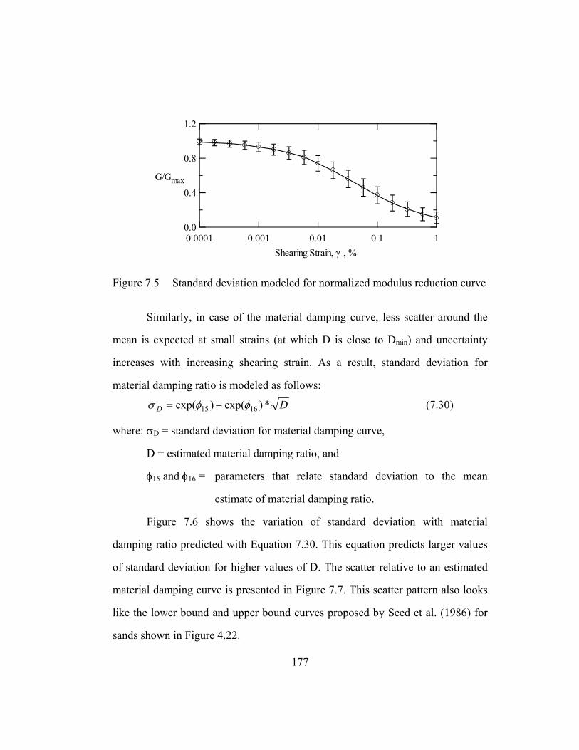
177
1.2
0.8
0.4
0.0
G/Gmax
0.0001 0.001 0.01 0.1 1Shearing Strain, γ , %
Figure 7.5 Standard deviation modeled for normalized modulus reduction curve
Similarly, in case of the material damping curve, less scatter around the
mean is expected at small strains (at which D is close to Dmin) and uncertainty
increases with increasing shearing strain. As a result, standard deviation for
material damping ratio is modeled as follows:
DD *)exp()exp( 1615 φφσ += (7.30)
where: σD = standard deviation for material damping curve,
D = estimated material damping ratio, and
φ15 and φ16 = parameters that relate standard deviation to the mean
estimate of material damping ratio.
Figure 7.6 shows the variation of standard deviation with material
damping ratio predicted with Equation 7.30. This equation predicts larger values
of standard deviation for higher values of D. The scatter relative to an estimated
material damping curve is presented in Figure 7.7. This scatter pattern also looks
like the lower bound and upper bound curves proposed by Seed et al. (1986) for
sands shown in Figure 4.22.

178
4
3
2
1
0
σD
2520151050D, %
Figure 7.6 Variation of standard deviation with material damping ratio
25
20
15
10
5
0
D , %
0.0001 0.001 0.01 0.1 1Shearing Strain, γ , %
Figure 7.7 Standard deviation modeled for material damping curve
Random variability and correlation between measurements are also
modeled in this study.
Due to equipment and operator errors, limited resolution of test equipment
and electronic noise that reduces measurement quality and precision, the result of
a test may not exactly be reproduced even though another test is performed under
identical circumstances. Measurements performed on the same specimen at the

179
same confining pressure using the same testing method are assumed to be
correlated. This correlation is modeled through using scale of fluctuation about
the mean estimate. Measurements performed at similar strain amplitudes are
modeled to be highly correlated with each other. The covariance structure is
formulated using:
))exp(
lnlnexp(*)
)exp(1exp(
1817, φ
γγ
φρ ji
ji
−−−= (7.31)
where: ρi,j = correlation coefficient,
γi = shearing strain at which measurement i is performed,
φ17 = random variability of data, and
φ18 = scale of fluctuation of data about the mean estimate.
7.5 SUMMARY
In this chapter, the First-order, Second-moment Bayesian Method is
introduced. This method is an approximation of Bayes’ theorem, which is a
systematic way of utilizing experience and observations in statistical analysis.
Equations that relate each parameter of the soil model to soil type and
loading conditions are also presented herein. The equations are formulated so that
the impact of strain amplitude, effective isotropic confining pressure, loading
history and loading frequency on dynamic soil behavior can be properly modeled
following the trends discussed in Chapter Four.
Finally, the equations formulated to represent the scatter and covariance
structure of the data are presented near the end of the chapter.
180
CHAPTER 8
STATISTICAL ANALYSIS OF THE RCTS DATA
8.1 INTRODUCTION
The statistical analysis of the RCTS data is performed using the First-
order, Second-moment Bayesian Method (FSBM) discussed in Chapter Seven. A
computer program that utilizes FSBM originally written by Dr. Robert B. Gilbert
is used in the analysis to calibrate the set of equations presented in Section 7.4.
The program was customized for this application through the C++ header and
source files presented in Appendices A through D.
Since the effect of number of cycles, N, and loading frequency, f, on
normalized modulus reduction curve is negligible in the case of the competent
soils that were investigated in the course of this study, the proposed equations in
Section 7.4 ignore the effect of N and f on G/Gmax. As a result, only resonant
column data (which is typically collected over a wider range of shearing strain
than the torsional shear test results) are utilized in the analysis of modulus
reduction. In case of material damping ratio, the proposed equations are calibrated
using the first and tenth cycles of torsional shear data along with the resonant
column data in an effort to model the effect of N and f on material damping ratio.
Since soil type is expected to be one of the most important parameters that
impact nonlinear soil behavior, the data was analyzed in several subsets according
to soil type and geographic location. Table 8.1 presents the distribution of the
specimens within the database according to soil type and geographic location. The
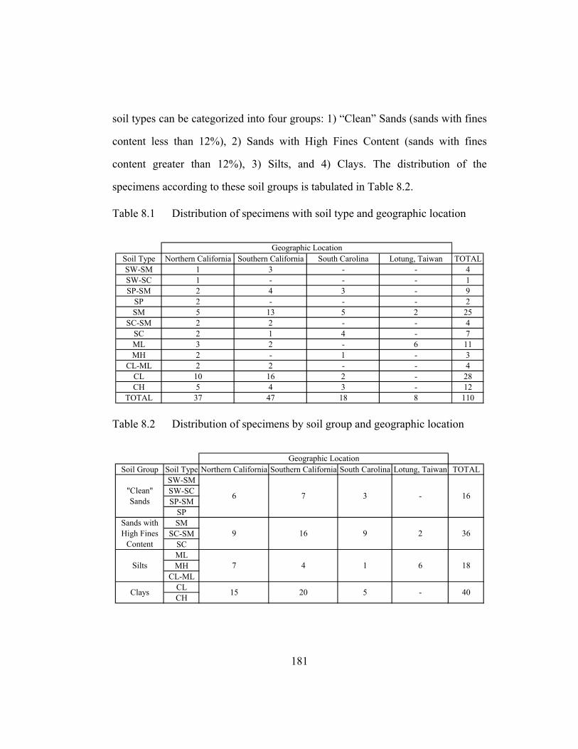
181
soil types can be categorized into four groups: 1) “Clean” Sands (sands with fines
content less than 12%), 2) Sands with High Fines Content (sands with fines
content greater than 12%), 3) Silts, and 4) Clays. The distribution of the
specimens according to these soil groups is tabulated in Table 8.2.
Table 8.1 Distribution of specimens with soil type and geographic location
Soil Type Northern California Southern California South Carolina Lotung, Taiwan TOTALSW-SM 1 3 - - 4SW-SC 1 - - - 1SP-SM 2 4 3 - 9
SP 2 - - - 2SM 5 13 5 2 25
SC-SM 2 2 - - 4SC 2 1 4 - 7ML 3 2 - 6 11MH 2 - 1 - 3
CL-ML 2 2 - - 4CL 10 16 2 - 28CH 5 4 3 - 12
TOTAL 37 47 18 8 110
Geographic Location
Table 8.2 Distribution of specimens by soil group and geographic location
Soil Group Soil Type Northern California Southern California South Carolina Lotung, Taiwan TOTALSW-SMSW-SCSP-SM
SPSM
SC-SMSCMLMH
CL-MLCLCH
16
36
18
40
61
5 -
Silts
Clays
6 7
9
7
15
16
4
20
Geographic Location
"Clean" Sands
Sands with High Fines
Content
3 -
9 2

182
The test results of all specimens from each soil group within a geographic
location were analyzed separately in order to study the effect of geology on model
parameters. Four specimens from South Carolina (specimens UT-39-G, UT-39-
M, UT-39-O, and UT-39-S) were removed from the database following the
analysis because the resonant column results did not follow the general trends
reported in the literature and observed during the course of this study. The
torsional shear results for these soils did follow the general trends but were not of
sufficient strain range to be included. As a result, a second set of analyses was
performed on two soil groups from which data had been discarded. Tables 8.3 and
8.4 present the distribution of the specimens within the database after the four
specimens have been discarded.
Table 8.3 Distribution of specimens with soil type and geographic location for the updated database
Soil Type Northern California Southern California South Carolina Lotung, Taiwan TOTALSW-SM 1 3 - - 4SW-SC 1 - - - 1SP-SM 2 4 3 - 9
SP 2 - - - 2SM 5 13 4 2 24
SC-SM 2 2 - - 4SC 2 1 3 - 6ML 3 2 - 6 11MH 2 - 1 - 3
CL-ML 2 2 - - 4CL 10 16 - - 26CH 5 4 3 - 12
TOTAL 37 47 14 8 106
Geographic Location

183
Table 8.4 Distribution of specimens by soil group and geographic location for the updated database
Soil Group Soil Type Northern California Southern California South Carolina Lotung, Taiwan TOTALSW-SMSW-SCSP-SM
SPSM
SC-SMSCMLMH
CL-MLCLCH
6 18
Clays 15 20 3 - 38
Silts 7 4 1
16
Sands with High Fines
Content9 16 7 2 34
Geographic Location
"Clean" Sands 6 7 3 -
The test results of all specimens from each soil group (regardless of its
geographic location) were also analyzed in order to study the effect of soil type on
model parameters. These analyses were performed on the updated database (after
discarding test results of the four specimens from South Carolina).
After concluding that the data were being stretched too thin to calibrate the
model using the subsets, the complete database was utilized in the analysis.
Section 8.3 presents the analysis of all credible data (within the updated database),
which forms the basis of the following chapters regarding the predictions based
on the calibrated model.
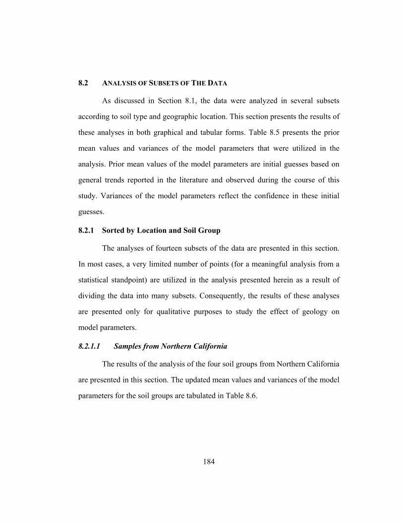
184
8.2 ANALYSIS OF SUBSETS OF THE DATA
As discussed in Section 8.1, the data were analyzed in several subsets
according to soil type and geographic location. This section presents the results of
these analyses in both graphical and tabular forms. Table 8.5 presents the prior
mean values and variances of the model parameters that were utilized in the
analysis. Prior mean values of the model parameters are initial guesses based on
general trends reported in the literature and observed during the course of this
study. Variances of the model parameters reflect the confidence in these initial
guesses.
8.2.1 Sorted by Location and Soil Group
The analyses of fourteen subsets of the data are presented in this section.
In most cases, a very limited number of points (for a meaningful analysis from a
statistical standpoint) are utilized in the analysis presented herein as a result of
dividing the data into many subsets. Consequently, the results of these analyses
are presented only for qualitative purposes to study the effect of geology on
model parameters.
8.2.1.1 Samples from Northern California
The results of the analysis of the four soil groups from Northern California
are presented in this section. The updated mean values and variances of the model
parameters for the soil groups are tabulated in Table 8.6.
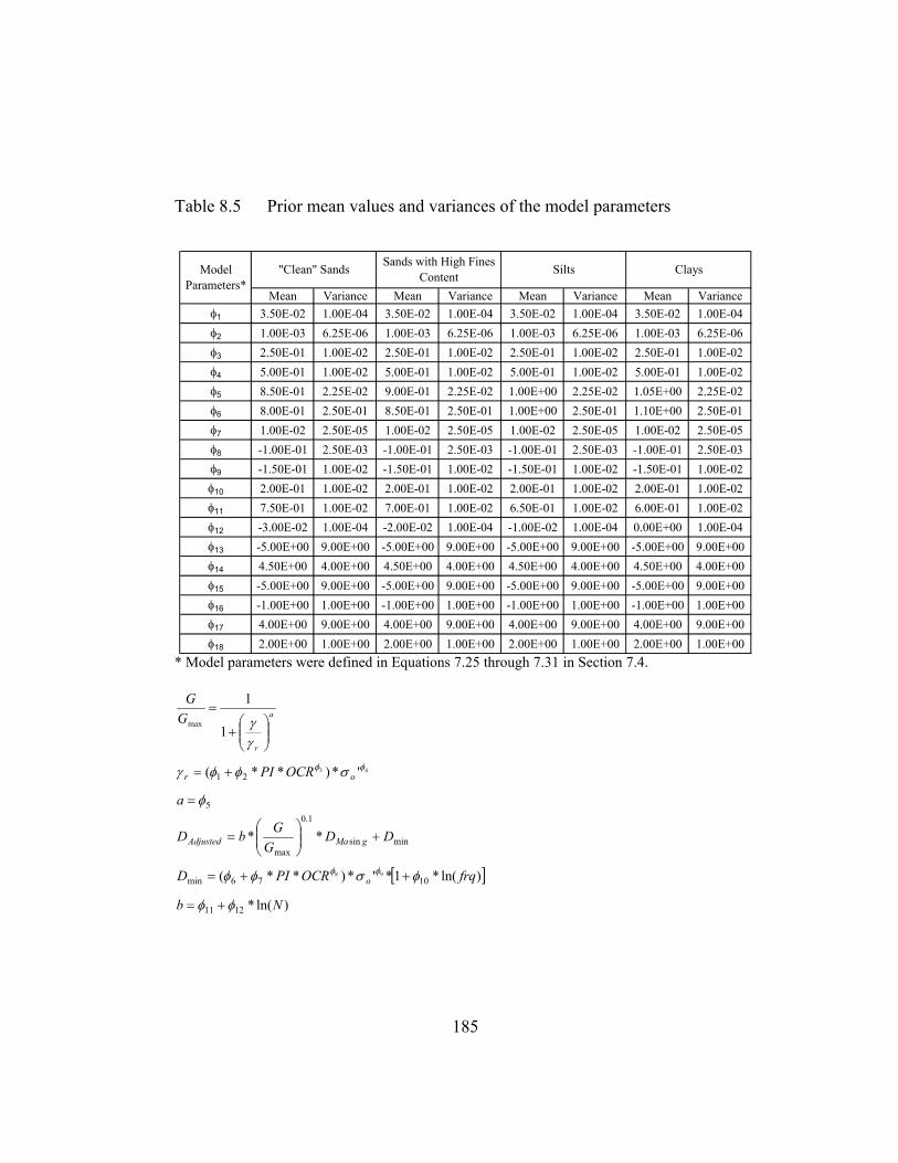
185
Table 8.5 Prior mean values and variances of the model parameters
Mean Variance Mean Variance Mean Variance Mean Varianceφ1 3.50E-02 1.00E-04 3.50E-02 1.00E-04 3.50E-02 1.00E-04 3.50E-02 1.00E-04φ2 1.00E-03 6.25E-06 1.00E-03 6.25E-06 1.00E-03 6.25E-06 1.00E-03 6.25E-06φ3 2.50E-01 1.00E-02 2.50E-01 1.00E-02 2.50E-01 1.00E-02 2.50E-01 1.00E-02φ4 5.00E-01 1.00E-02 5.00E-01 1.00E-02 5.00E-01 1.00E-02 5.00E-01 1.00E-02φ5 8.50E-01 2.25E-02 9.00E-01 2.25E-02 1.00E+00 2.25E-02 1.05E+00 2.25E-02φ6 8.00E-01 2.50E-01 8.50E-01 2.50E-01 1.00E+00 2.50E-01 1.10E+00 2.50E-01φ7 1.00E-02 2.50E-05 1.00E-02 2.50E-05 1.00E-02 2.50E-05 1.00E-02 2.50E-05φ8 -1.00E-01 2.50E-03 -1.00E-01 2.50E-03 -1.00E-01 2.50E-03 -1.00E-01 2.50E-03φ9 -1.50E-01 1.00E-02 -1.50E-01 1.00E-02 -1.50E-01 1.00E-02 -1.50E-01 1.00E-02φ10 2.00E-01 1.00E-02 2.00E-01 1.00E-02 2.00E-01 1.00E-02 2.00E-01 1.00E-02φ11 7.50E-01 1.00E-02 7.00E-01 1.00E-02 6.50E-01 1.00E-02 6.00E-01 1.00E-02φ12 -3.00E-02 1.00E-04 -2.00E-02 1.00E-04 -1.00E-02 1.00E-04 0.00E+00 1.00E-04φ13 -5.00E+00 9.00E+00 -5.00E+00 9.00E+00 -5.00E+00 9.00E+00 -5.00E+00 9.00E+00φ14 4.50E+00 4.00E+00 4.50E+00 4.00E+00 4.50E+00 4.00E+00 4.50E+00 4.00E+00φ15 -5.00E+00 9.00E+00 -5.00E+00 9.00E+00 -5.00E+00 9.00E+00 -5.00E+00 9.00E+00φ16 -1.00E+00 1.00E+00 -1.00E+00 1.00E+00 -1.00E+00 1.00E+00 -1.00E+00 1.00E+00φ17 4.00E+00 9.00E+00 4.00E+00 9.00E+00 4.00E+00 9.00E+00 4.00E+00 9.00E+00φ18 2.00E+00 1.00E+00 2.00E+00 1.00E+00 2.00E+00 1.00E+00 2.00E+00 1.00E+00
Model Parameters*
"Clean" Sands Sands with High Fines Content Silts Clays
* Model parameters were defined in Equations 7.25 through 7.31 in Section 7.4.
a
r
GG
+
=
γγ1
1
max
43 '*)**( 21φφ σφφγ or OCRPI+=
5φ=a
minsin
1.0
max** DD
GGbD gMaAdjusted +
=
[ ])ln(*1*'*)**( 1076min98 frqOCRPID o φσφφ φφ ++=
)ln(*1211 Nb φφ +=

186
Table 8.6 Updated mean values and variances of the model parameters for the soils from Northern California
Mean Variance Mean Variance Mean Variance Mean Varianceφ1 4.26E-02 9.50E-06 2.76E-02 2.05E-06 3.97E-02 8.49E-06 3.39E-02 3.65E-05φ2 -2.28E-03 1.20E-07 -3.42E-05 8.90E-09 -3.27E-06 4.25E-08 1.75E-03 5.30E-08φ3 2.50E-01 1.00E-02 2.50E-01 1.00E-02 2.50E-01 1.00E-02 2.97E-01 4.62E-03φ4 2.53E-01 1.90E-03 2.49E-01 1.26E-03 1.50E-01 1.41E-03 2.78E-01 1.07E-03φ5 9.41E-01 6.28E-04 8.83E-01 2.33E-04 1.05E+00 8.37E-04 9.93E-01 4.66E-04φ6 9.95E-01 1.25E-02 1.26E+00 2.19E-02 9.54E-01 6.99E-03 1.05E+00 1.30E-02φ7 1.24E-02 2.37E-05 1.61E-02 2.21E-05 8.04E-03 1.95E-05 8.20E-04 1.05E-05φ8 -1.00E-01 2.50E-03 -1.00E-01 2.50E-03 -9.95E-02 2.50E-03 -1.01E-01 2.50E-03φ9 1.25E-01 5.15E-03 -1.73E-01 3.56E-03 -2.30E-01 2.40E-03 -1.72E-01 1.67E-03φ10 2.85E-01 3.37E-03 2.19E-01 2.09E-03 2.90E-01 3.59E-03 3.23E-01 2.98E-03φ11 7.50E-01 1.96E-03 6.71E-01 1.09E-03 4.11E-01 6.93E-04 4.40E-01 5.99E-04φ12 -2.83E-02 3.40E-05 -1.50E-02 3.28E-05 1.58E-02 1.81E-05 2.33E-02 1.61E-05φ13 -3.70E+00 7.49E-02 -3.35E+00 1.76E-02 -5.00E+00 9.00E+00 -5.28E+00 1.27E-01φ14 4.71E+00 3.07E-01 5.11E+00 3.50E+00 4.31E+00 6.40E-02 3.89E+00 4.45E-02φ15 -5.03E+00 8.97E+00 -5.06E+00 8.90E+00 -5.01E+00 8.99E+00 -5.22E+00 8.75E+00φ16 -5.02E-01 1.39E-02 -4.29E-01 1.14E-02 -9.62E-01 1.01E-02 -6.70E-01 6.16E-03φ17 4.85E+00 2.14E-01 3.79E+00 9.24E-02 4.03E+00 8.98E+00 7.04E+00 6.66E-01φ18 2.95E+00 6.66E-02 2.67E+00 5.89E-02 1.94E+00 4.60E-02 2.18E+00 2.52E-02
Silts ClaysModel Parameters*
"Clean" Sands Sands with High Fines Content
* Model parameters were defined in Equations 7.25 through 7.31 in Section 7.4.
a
r
GG
+
=
γγ1
1
max
43 '*)**( 21φφ σφφγ or OCRPI+=
5φ=a
minsin
1.0
max** DD
GGbD gMaAdjusted +
=
[ ])ln(*1*'*)**( 1076min98 frqOCRPID o φσφφ φφ ++=
)ln(*1211 Nb φφ +=

187
Since most of the specimens from Northern California are normally
consolidated, the updated mean values and variances of φ3 and φ8 (which
represent the effect of overconsolidation ratio on reference strain and small-strain
material damping ratio, respectively) are almost identical to prior values. Hence,
the data have not provided much information regarding these parameters. The
values of φ1 (which represents the reference strain of a nonplastic soil at 1 atm
confining pressure), φ4 (which represents the effect of confining pressure on
reference strain), φ6 (which represents the small-strain material damping ratio of a
nonplastic soil at 1 atm confining pressure deformed at 1 Hz loading frequency)
and φ10 (which represents the effect of loading frequency on small-strain material
damping ratio) are observed to be consistent between soil groups.
The comparisons of the measurements with the predicted values based on
the calibrated models for the four soil groups are presented in Figures 8.1 through
8.4. Significantly less error is observed in the prediction of normalized shear
modulus than in the prediction of material damping predictions ratio for all soil
groups. This difference can be attributed to material damping ratio being sensitive
to the characteristics of the complete stress-strain loop while normalized shear
modulus is only related to the end points of the stress-strain loop. Consequently,
measurement and prediction of material damping ratio is more complicated than
measurement and prediction of normalized shear modulus.

188
1.2
1.0
0.8
0.6
0.4
0.2
0.0Pred
icte
d N
orm
aliz
ed M
odul
us
1.21.00.80.60.40.20.0
Measured Normalized Modulus
(a)25
20
15
10
5
0
Pred
icte
d M
ater
ial D
ampi
ng
2520151050
Measured Material Damping
(b)
Figure 8.1 Comparisons of the measured and predicted values of (a) normalized modulus and (b) material damping ratio for “clean” sands from Northern California
1.2
1.0
0.8
0.6
0.4
0.2
0.0Pred
icte
d N
orm
aliz
ed M
odul
us
1.21.00.80.60.40.20.0
Measured Normalized Modulus
(a)25
20
15
10
5
0
Pred
icte
d M
ater
ial D
ampi
ng
2520151050
Measured Material Damping
(b)
Figure 8.2 Comparisons of the measured and predicted values of (a) normalized modulus and (b) material damping ratio for sands with high fines content from Northern California
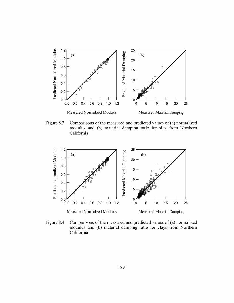
189
1.2
1.0
0.8
0.6
0.4
0.2
0.0Pred
icte
d N
orm
aliz
ed M
odul
us
1.21.00.80.60.40.20.0
Measured Normalized Modulus
(a)25
20
15
10
5
0
Pred
icte
d M
ater
ial D
ampi
ng
2520151050
Measured Material Damping
(b)
Figure 8.3 Comparisons of the measured and predicted values of (a) normalized modulus and (b) material damping ratio for silts from Northern California
1.2
1.0
0.8
0.6
0.4
0.2
0.0Pred
icte
d N
orm
aliz
ed M
odul
us
1.21.00.80.60.40.20.0
Measured Normalized Modulus
(a)25
20
15
10
5
0
Pred
icte
d M
ater
ial D
ampi
ng
2520151050
Measured Material Damping
(b)
Figure 8.4 Comparisons of the measured and predicted values of (a) normalized modulus and (b) material damping ratio for clays from Northern California

190
8.2.1.2 Samples from Southern California
The updated mean values and variances of the model parameters for the
four soil groups from Southern California are tabulated in Table 8.7. As in the
case of Northern California, the data have not provided much information
regarding the φ3 and φ8 parameters. The φ1, φ4, φ6 and φ10 parameters are again
observed to be consistent between soil groups. φ5 (which is the curvature
coefficient) is observed to slightly increase with decreasing particle size. The
comparisons of the measured and predicted values based on the calibrated models
are presented in Figures 8.5 through 8.8.
8.2.1.3 Samples from South Carolina
8.2.1.3.1 Analysis of Test Results from All (Eighteen) Specimens
The updated mean values and variances of the model parameters for the
four soil groups from South Carolina are tabulated in Table 8.8. The model
parameters are observed to be extremely inconsistent. Part of the problem is
believed to be the result of analyzing a very small dataset in the case of “clean”
sands and silts.
The comparisons of the measured and predicted values based on the
calibrated models are presented in Figures 8.9 through 8.12. Test results from four
specimens do not agree with the observed trends and reduce the quality of the
predictions for two soil groups, sands with high fines content and clays. As a
result, these specimens were identified and discarded from the database.
191
Table 8.7 Updated mean values and variances of the model parameters for the soils from Southern California
Mean Variance Mean Variance Mean Variance Mean Varianceφ1 2.53E-02 6.44E-06 3.51E-02 5.30E-06 5.18E-02 4.53E-05 3.52E-02 5.76E-06φ2 1.00E-03 6.25E-06 1.34E-03 8.41E-08 5.96E-05 9.19E-07 7.07E-04 9.12E-09φ3 2.50E-01 1.00E-02 2.62E-01 9.44E-03 2.50E-01 1.00E-02 3.69E-01 7.30E-03φ4 4.62E-01 2.97E-03 5.04E-01 1.35E-03 4.26E-01 9.34E-04 2.97E-01 5.31E-04φ5 8.34E-01 6.37E-04 8.58E-01 3.62E-04 9.40E-01 1.41E-03 9.50E-01 2.25E-04φ6 8.42E-01 3.56E-02 8.26E-01 1.19E-02 7.75E-01 7.47E-03 1.01E+00 4.39E-03φ7 1.00E-02 2.50E-05 1.29E-02 2.36E-05 8.55E-03 2.41E-05 3.92E-04 1.06E-05φ8 -1.00E-01 2.50E-03 -1.00E-01 2.50E-03 -1.00E-01 2.50E-03 -1.01E-01 2.49E-03φ9 -2.90E-01 6.32E-03 -4.18E-01 2.99E-03 -1.30E-01 1.50E-03 -1.97E-01 9.35E-04φ10 2.53E-01 5.59E-03 2.37E-01 2.70E-03 1.97E-01 2.90E-03 3.74E-01 1.76E-03φ11 7.62E-01 2.08E-03 7.70E-01 1.61E-03 6.67E-01 2.24E-03 5.18E-01 4.84E-04φ12 -2.67E-02 4.19E-05 -2.41E-02 3.12E-05 -1.95E-02 3.56E-05 1.68E-02 1.18E-05φ13 -5.05E+00 8.93E+00 -5.00E+00 9.00E+00 -5.02E+00 8.98E+00 -5.68E+00 3.93E-02φ14 4.51E+00 6.15E-02 3.27E+00 3.49E-02 4.92E+00 8.97E-02 4.39E+00 1.98E-02φ15 -5.00E+00 9.00E+00 -5.04E+00 8.96E+00 -5.00E+00 9.00E+00 -5.03E+00 8.97E+00φ16 -5.97E-01 1.38E-02 -1.81E-01 7.62E-03 -1.23E+00 1.54E-02 -8.40E-01 2.98E-03φ17 3.99E+00 9.00E+00 4.00E+00 9.00E+00 4.06E+00 8.93E+00 4.23E+00 8.80E+00φ18 2.19E+00 5.19E-02 2.80E+00 2.65E-02 1.53E+00 8.08E-02 2.08E+00 1.31E-02
"Clean" Sands Sands with High Fines Content Silts ClaysModel
Parameters*
* Model parameters were defined in Equations 7.25 through 7.31 in Section 7.4.
a
r
GG
+
=
γγ1
1
max
43 '*)**( 21φφ σφφγ or OCRPI+=
5φ=a
minsin
1.0
max** DD
GGbD gMaAdjusted +
=
[ ])ln(*1*'*)**( 1076min98 frqOCRPID o φσφφ φφ ++=
)ln(*1211 Nb φφ +=

192
1.2
1.0
0.8
0.6
0.4
0.2
0.0Pred
icte
d N
orm
aliz
ed M
odul
us
1.21.00.80.60.40.20.0
Measured Normalized Modulus
(a)25
20
15
10
5
0
Pred
icte
d M
ater
ial D
ampi
ng
2520151050
Measured Material Damping
(b)
Figure 8.5 Comparisons of the measured and predicted values of (a) normalized modulus and (b) material damping ratio for “clean” sands from Southern California
1.2
1.0
0.8
0.6
0.4
0.2
0.0Pred
icte
d N
orm
aliz
ed M
odul
us
1.21.00.80.60.40.20.0
Measured Normalized Modulus
(a)25
20
15
10
5
0
Pred
icte
d M
ater
ial D
ampi
ng
2520151050
Measured Material Damping
(b)
Figure 8.6 Comparisons of the measured and predicted values of (a) normalized modulus and (b) material damping ratio for sands with high fines content from Southern California

193
1.2
1.0
0.8
0.6
0.4
0.2
0.0Pred
icte
d N
orm
aliz
ed M
odul
us
1.21.00.80.60.40.20.0
Measured Normalized Modulus
(a)25
20
15
10
5
0
Pred
icte
d M
ater
ial D
ampi
ng
2520151050
Measured Material Damping
(b)
Figure 8.7 Comparisons of the measured and predicted values of (a) normalized modulus and (b) material damping ratio for silts from Southern California
1.2
1.0
0.8
0.6
0.4
0.2
0.0Pred
icte
d N
orm
aliz
ed M
odul
us
1.21.00.80.60.40.20.0
Measured Normalized Modulus
(a)25
20
15
10
5
0
Pred
icte
d M
ater
ial D
ampi
ng
2520151050
Measured Material Damping
(b)
Figure 8.8 Comparisons of the measured and predicted values of (a) normalized modulus and (b) material damping ratio for clays from Southern California

194
Table 8.8 Updated mean values and variances of the model parameters for the soils from South Carolina
Mean Variance Mean Variance Mean Variance Mean Varianceφ1 6.83E-02 3.33E-05 3.22E-02 2.32E-05 3.47E-02 9.99E-05 3.20E-02 9.90E-05φ2 5.82E-03 5.21E-06 -5.03E-04 7.03E-08 9.34E-04 9.82E-09 2.79E-03 2.90E-07φ3 2.50E-01 1.00E-02 2.50E-01 1.00E-02 2.83E-01 9.88E-03 2.50E-01 1.00E-02φ4 -3.88E-01 2.85E-03 -3.80E-02 3.52E-03 2.30E-01 1.98E-03 7.04E-02 1.92E-03φ5 8.38E-01 6.73E-03 8.96E-01 1.87E-03 1.17E+00 2.18E-03 1.09E+00 5.85E-03φ6 1.57E-01 5.13E-05 2.82E-01 1.47E-03 5.13E-01 1.40E-01 -2.18E-01 8.59E-02φ7 1.01E-02 2.49E-05 1.68E-02 1.00E-05 4.90E-03 9.65E-06 5.70E-03 1.24E-05φ8 -1.00E-01 2.50E-03 -9.87E-02 2.50E-03 -1.12E-01 2.10E-03 -1.00E-01 2.50E-03φ9 -1.46E-01 6.68E-03 4.71E-02 6.16E-03 -1.25E-01 4.22E-03 -2.93E-01 7.83E-03φ10 2.27E-01 1.26E-03 3.05E-01 8.95E-03 9.62E-02 8.47E-04 1.42E-01 5.69E-03φ11 8.87E-01 2.36E-03 6.68E-01 3.05E-03 4.35E-01 1.12E-03 3.53E-01 4.25E-03φ12 -1.26E-02 3.76E-05 -2.05E-02 4.69E-05 2.32E-02 3.22E-05 -2.08E-02 7.07E-05φ13 -6.57E+00 6.41E-01 -5.04E+00 8.97E+00 -5.84E+00 3.42E-01 -4.65E+00 1.01E-01φ14 5.38E+00 2.88E-01 2.44E+00 7.23E-02 5.98E+00 3.14E-01 3.94E+00 2.88E-01φ15 -5.00E+00 9.00E+00 -5.00E+00 9.00E+00 -5.02E+00 8.98E+00 -5.00E+00 9.00E+00φ16 -1.80E+00 1.43E-02 -1.20E-01 1.75E-02 -1.59E+00 1.11E-02 8.52E-01 3.96E-02φ17 3.36E+00 5.19E-01 4.00E+00 9.00E+00 4.01E+00 8.99E+00 4.03E+00 8.98E+00φ18 5.66E-01 8.76E-02 2.39E+00 5.09E-02 -3.42E-03 8.17E-02 2.82E+00 1.00E-01
"Clean" Sands Sands with High Fines Content Silts ClaysModel
Parameters*
* Model parameters were defined in Equations 7.25 through 7.31 in Section 7.4.
a
r
GG
+
=
γγ1
1
max
43 '*)**( 21φφ σφφγ or OCRPI+=
5φ=a
minsin
1.0
max** DD
GGbD gMaAdjusted +
=
[ ])ln(*1*'*)**( 1076min98 frqOCRPID o φσφφ φφ ++=
)ln(*1211 Nb φφ +=
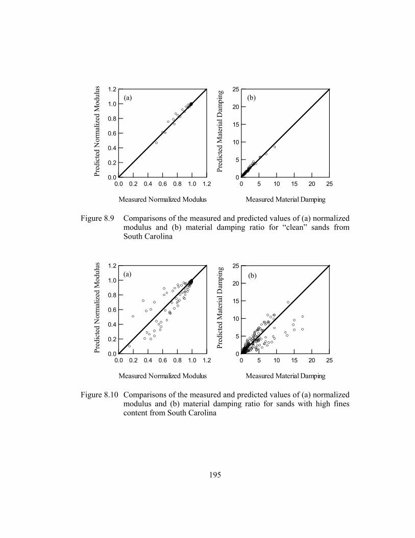
195
1.2
1.0
0.8
0.6
0.4
0.2
0.0Pred
icte
d N
orm
aliz
ed M
odul
us
1.21.00.80.60.40.20.0
Measured Normalized Modulus
(a)25
20
15
10
5
0
Pred
icte
d M
ater
ial D
ampi
ng
2520151050
Measured Material Damping
(b)
Figure 8.9 Comparisons of the measured and predicted values of (a) normalized modulus and (b) material damping ratio for “clean” sands from South Carolina
1.2
1.0
0.8
0.6
0.4
0.2
0.0Pred
icte
d N
orm
aliz
ed M
odul
us
1.21.00.80.60.40.20.0
Measured Normalized Modulus
(a)25
20
15
10
5
0
Pred
icte
d M
ater
ial D
ampi
ng
2520151050
Measured Material Damping
(b)
Figure 8.10 Comparisons of the measured and predicted values of (a) normalized modulus and (b) material damping ratio for sands with high fines content from South Carolina

196
1.2
1.0
0.8
0.6
0.4
0.2
0.0Pred
icte
d N
orm
aliz
ed M
odul
us
1.21.00.80.60.40.20.0
Measured Normalized Modulus
(a)25
20
15
10
5
0
Pred
icte
d M
ater
ial D
ampi
ng
2520151050
Measured Material Damping
(b)
Figure 8.11 Comparisons of the measured and predicted values of (a) normalized modulus and (b) material damping ratio for silts from South Carolina
1.2
1.0
0.8
0.6
0.4
0.2
0.0Pred
icte
d N
orm
aliz
ed M
odul
us
1.21.00.80.60.40.20.0
Measured Normalized Modulus
(a)25
20
15
10
5
0
Pred
icte
d M
ater
ial D
ampi
ng
2520151050
Measured Material Damping
(b)
Figure 8.12 Comparisons of the measured and predicted values of (a) normalized modulus and (b) material damping ratio for clays from South Carolina
197
8.2.1.3.2 Analysis of Test Results from Fourteen Specimens
After discarding the four specimens that were identified not to be
consistent with the observed trends, the two soil groups (sands with high fines
content and clays) that were affected by the process of changing the contents of
the database were reevaluated. Considerable improvement in predicted values is
achieved. The updated mean values and variances of the model parameters for
these two soil groups from South Carolina are tabulated in Table 8.9 and the
comparisons of the measured and predicted values based on the calibrated models
are presented in Figures 8.13 through 8.14.
8.2.1.4 Samples from Lotung, Taiwan
The updated mean values and variances of the model parameters for the
two soil groups from Lotung, Taiwan are tabulated in Table 8.10. Inconsistencies
between the model parameters are attributed to analyzing a very small dataset in
the case of sands with high fines content. The comparisons of the measured and
predicted values based on the calibrated models are presented in Figures 8.15 and
8.16.
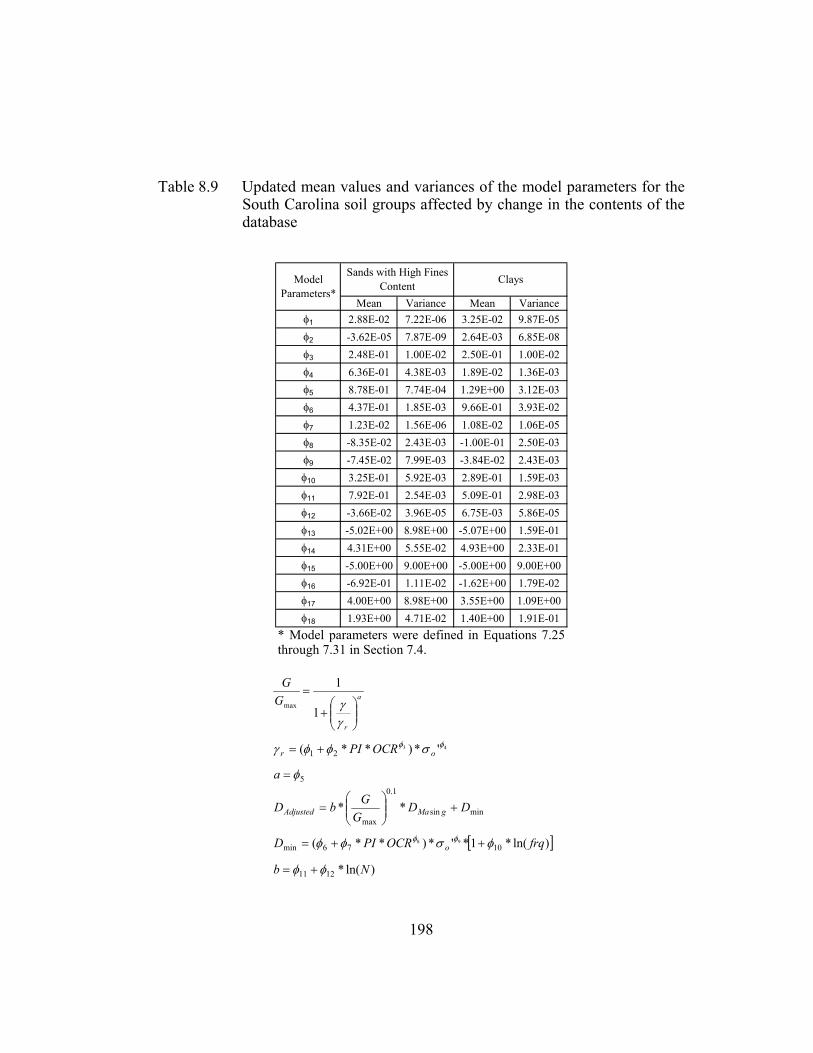
198
Table 8.9 Updated mean values and variances of the model parameters for the South Carolina soil groups affected by change in the contents of the database
Mean Variance Mean Varianceφ1 2.88E-02 7.22E-06 3.25E-02 9.87E-05φ2 -3.62E-05 7.87E-09 2.64E-03 6.85E-08φ3 2.48E-01 1.00E-02 2.50E-01 1.00E-02φ4 6.36E-01 4.38E-03 1.89E-02 1.36E-03φ5 8.78E-01 7.74E-04 1.29E+00 3.12E-03φ6 4.37E-01 1.85E-03 9.66E-01 3.93E-02φ7 1.23E-02 1.56E-06 1.08E-02 1.06E-05φ8 -8.35E-02 2.43E-03 -1.00E-01 2.50E-03φ9 -7.45E-02 7.99E-03 -3.84E-02 2.43E-03φ10 3.25E-01 5.92E-03 2.89E-01 1.59E-03φ11 7.92E-01 2.54E-03 5.09E-01 2.98E-03φ12 -3.66E-02 3.96E-05 6.75E-03 5.86E-05φ13 -5.02E+00 8.98E+00 -5.07E+00 1.59E-01φ14 4.31E+00 5.55E-02 4.93E+00 2.33E-01φ15 -5.00E+00 9.00E+00 -5.00E+00 9.00E+00φ16 -6.92E-01 1.11E-02 -1.62E+00 1.79E-02φ17 4.00E+00 8.98E+00 3.55E+00 1.09E+00φ18 1.93E+00 4.71E-02 1.40E+00 1.91E-01
Sands with High Fines Content ClaysModel
Parameters*
* Model parameters were defined in Equations 7.25 through 7.31 in Section 7.4.
a
r
GG
+
=
γγ1
1
max
43 '*)**( 21φφ σφφγ or OCRPI+=
5φ=a
minsin
1.0
max** DD
GGbD gMaAdjusted +
=
[ ])ln(*1*'*)**( 1076min98 frqOCRPID o φσφφ φφ ++=
)ln(*1211 Nb φφ +=
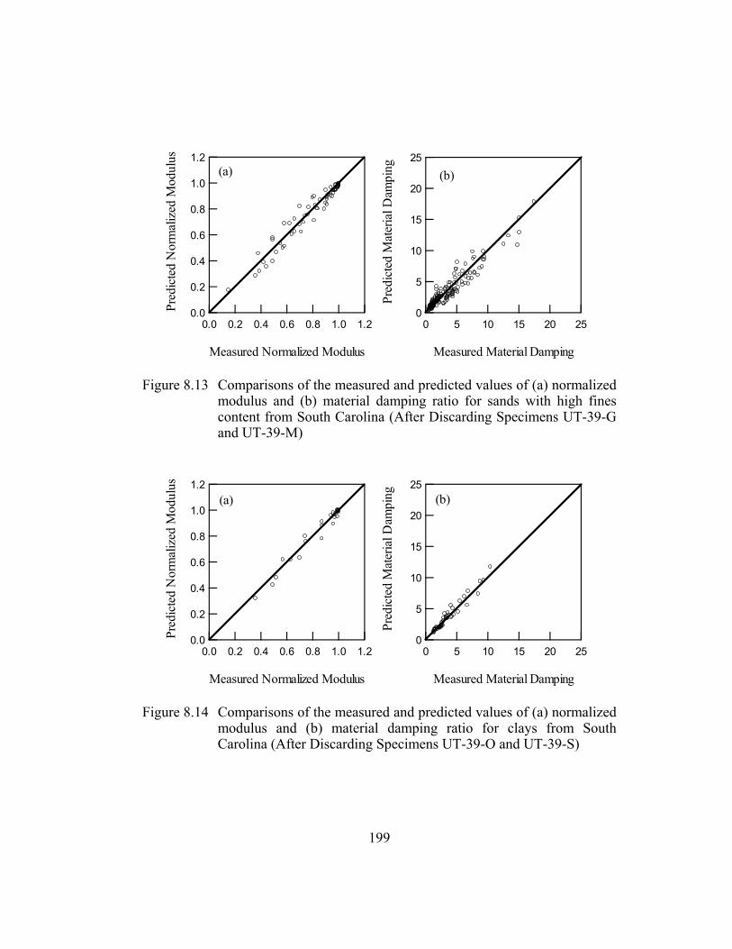
199
1.2
1.0
0.8
0.6
0.4
0.2
0.0Pred
icte
d N
orm
aliz
ed M
odul
us
1.21.00.80.60.40.20.0
Measured Normalized Modulus
(a)25
20
15
10
5
0
Pred
icte
d M
ater
ial D
ampi
ng
2520151050
Measured Material Damping
(b)
Figure 8.13 Comparisons of the measured and predicted values of (a) normalized modulus and (b) material damping ratio for sands with high fines content from South Carolina (After Discarding Specimens UT-39-G and UT-39-M)
1.2
1.0
0.8
0.6
0.4
0.2
0.0Pred
icte
d N
orm
aliz
ed M
odul
us
1.21.00.80.60.40.20.0
Measured Normalized Modulus
(a)25
20
15
10
5
0
Pred
icte
d M
ater
ial D
ampi
ng
2520151050
Measured Material Damping
(b)
Figure 8.14 Comparisons of the measured and predicted values of (a) normalized modulus and (b) material damping ratio for clays from South Carolina (After Discarding Specimens UT-39-O and UT-39-S)
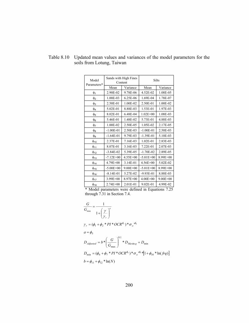
200
Table 8.10 Updated mean values and variances of the model parameters for the soils from Lotung, Taiwan
Mean Variance Mean Varianceφ1 2.90E-02 9.78E-06 4.52E-02 1.08E-05φ2 1.00E-03 6.25E-06 1.69E-04 1.78E-07φ3 2.50E-01 1.00E-02 2.50E-01 1.00E-02φ4 5.02E-01 8.88E-03 1.53E-01 1.97E-03φ5 8.02E-01 6.48E-04 1.02E+00 1.08E-03φ6 5.46E-01 1.48E-02 5.73E-01 4.88E-03φ7 1.00E-02 2.50E-05 1.05E-02 2.17E-05φ8 -1.00E-01 2.50E-03 -1.00E-01 2.50E-03φ9 -1.64E-01 9.79E-03 -1.39E-01 5.10E-03φ10 2.37E-01 7.16E-03 1.02E-01 2.83E-03φ11 8.07E-01 3.16E-03 7.22E-01 2.07E-03φ12 -3.84E-02 5.39E-05 -1.70E-02 2.89E-05φ13 -7.12E+00 4.55E+00 -5.01E+00 8.99E+00φ14 4.79E+00 3.14E-01 4.56E+00 5.02E-02φ15 -5.00E+00 9.00E+00 -5.01E+00 8.99E+00φ16 -8.14E-01 5.27E-02 -9.93E-01 8.88E-03φ17 3.99E+00 8.97E+00 4.00E+00 9.00E+00φ18 2.74E+00 2.01E-01 9.02E-01 4.99E-02
Sands with High Fines Content SiltsModel
Parameters*
* Model parameters were defined in Equations 7.25 through 7.31 in Section 7.4.
a
r
GG
+
=
γγ1
1
max
43 '*)**( 21φφ σφφγ or OCRPI+=
5φ=a
minsin
1.0
max** DD
GGbD gMaAdjusted +
=
[ ])ln(*1*'*)**( 1076min98 frqOCRPID o φσφφ φφ ++=
)ln(*1211 Nb φφ +=
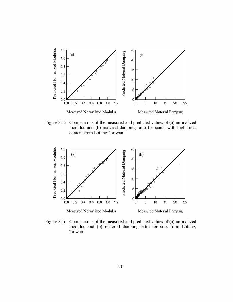
201
1.2
1.0
0.8
0.6
0.4
0.2
0.0Pred
icte
d N
orm
aliz
ed M
odul
us
1.21.00.80.60.40.20.0
Measured Normalized Modulus
(a)25
20
15
10
5
0
Pred
icte
d M
ater
ial D
ampi
ng
2520151050
Measured Material Damping
(b)
Figure 8.15 Comparisons of the measured and predicted values of (a) normalized modulus and (b) material damping ratio for sands with high fines content from Lotung, Taiwan
1.2
1.0
0.8
0.6
0.4
0.2
0.0Pred
icte
d N
orm
aliz
ed M
odul
us
1.21.00.80.60.40.20.0
Measured Normalized Modulus
(a)25
20
15
10
5
0
Pred
icte
d M
ater
ial D
ampi
ng
2520151050
Measured Material Damping
(b)
Figure 8.16 Comparisons of the measured and predicted values of (a) normalized modulus and (b) material damping ratio for silts from Lotung, Taiwan

202
8.2.1.5 Comparison of the Nonlinear Behavior of Soils from Different Locations
In order to evaluate the impact of geology on nonlinear soil behavior, the
normalized modulus reduction and material damping curves for a given soil type
under given loading conditions are predicted utilizing the updated model
parameters for different geographic locations. Figures 8.17 through 8.19 present
the comparison of these predictions.
In Figure 8.17, predicted normalized modulus reduction and material
damping curves for a silty sand are shown. The soil is selected to be nonplastic
and normally consolidated in order to analyze a representative material within the
database. The confining pressure is selected to be 1 atm in the same fashion. Ten
cycles of loading at 1 Hz is chosen so that the loading conditions represent the
characteristics of an earthquake. In this figure, the effect of geographic location
(and geology for that matter) on dynamic soil behavior is observed to be
negligible.
Figure 8.18 shows the comparison of predicted nonlinear soil behavior for
a moderate plasticity silt. The characteristics of the soil are again selected so that
a representative material within the database is evaluated. Loading conditions are
selected to be the same as those in the case of the silty sand. In Figure 8.18a,
normalized modulus reduction curves for the two predictions are observed to be
quite similar. On the other hand, the predicted material damping ratios shown in
Figure 8.18b are somewhat different at shearing strains above 0.1 %. This
divergence can be investigated in future studies using a larger database.

203
1.2
1.0
0.8
0.6
0.4
0.2
0.0
G/Gmax
(a)
Silty Sand from Northern CaliforniaSilty Sand from Southern CaliforniaSilty Sand from South Carolina
25
20
15
10
5
0
D, %
0.0001 0.001 0.01 0.1 1
Shearing Strain, γ ,%
(b)
PI = 0 %OCR = 1f = 1 HzN =10σo' = 1 atm
Figure 8.17 (a) Normalized modulus reduction and (b) material damping curves estimated for a nonplastic silty sand using updated mean values of model parameters calibrated at different geographic locations
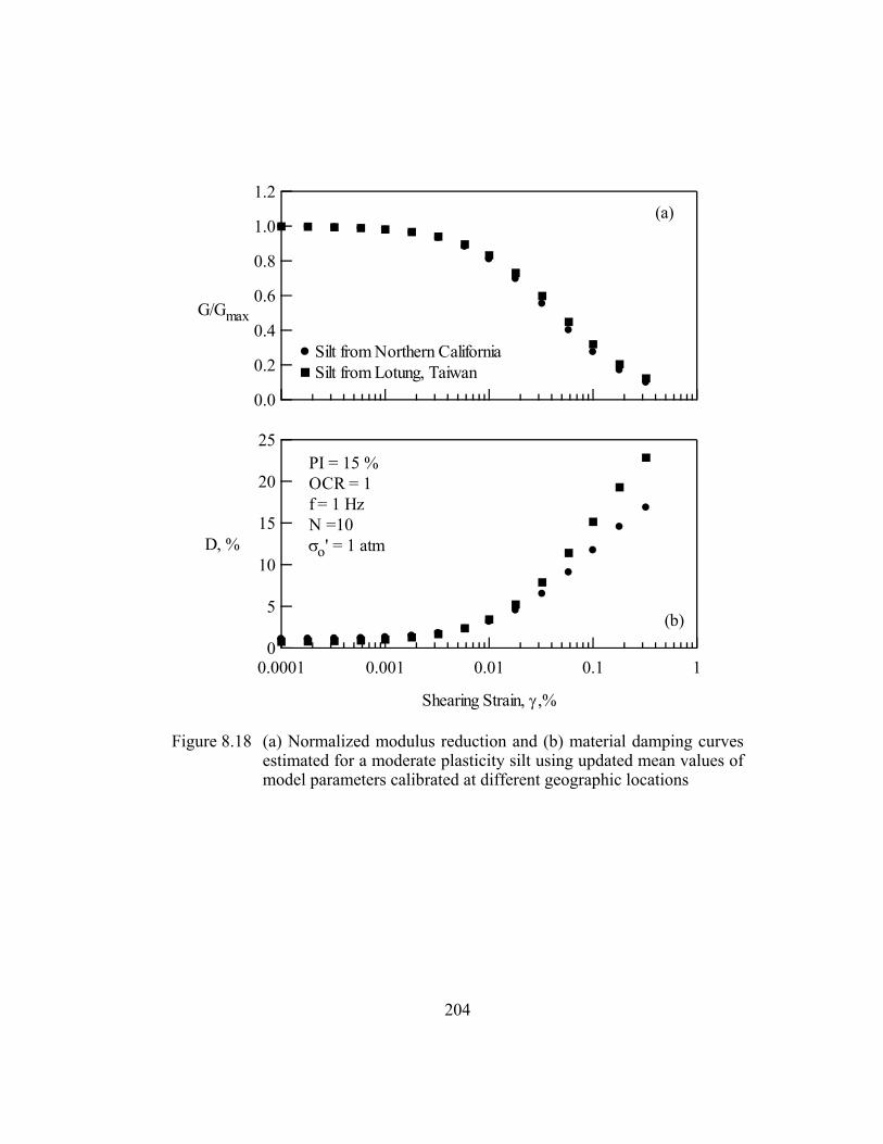
204
1.2
1.0
0.8
0.6
0.4
0.2
0.0
G/Gmax
(a)
Silt from Northern CaliforniaSilt from Lotung, Taiwan
25
20
15
10
5
0
D, %
0.0001 0.001 0.01 0.1 1
Shearing Strain, γ ,%
(b)
PI = 15 %OCR = 1f = 1 HzN =10σo' = 1 atm
Figure 8.18 (a) Normalized modulus reduction and (b) material damping curves estimated for a moderate plasticity silt using updated mean values of model parameters calibrated at different geographic locations
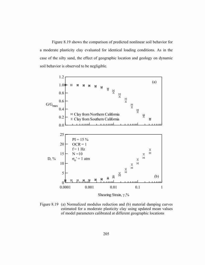
205
Figure 8.19 shows the comparison of predicted nonlinear soil behavior for
a moderate plasticity clay evaluated for identical loading conditions. As in the
case of the silty sand, the effect of geographic location and geology on dynamic
soil behavior is observed to be negligible.
1.2
1.0
0.8
0.6
0.4
0.2
0.0
G/Gmax
(a)
Clay from Northern CaliforniaClay from Southern California
25
20
15
10
5
0
D, %
0.0001 0.001 0.01 0.1 1
Shearing Strain, γ ,%
(b)
PI = 15 %OCR = 1f = 1 HzN =10σo' = 1 atm
Figure 8.19 (a) Normalized modulus reduction and (b) material damping curves estimated for a moderate plasticity clay using updated mean values of model parameters calibrated at different geographic locations

206
Comparison of the results for the subsets of the data sorted according to
geographic location does not indicate a strong correlation between geology and
nonlinear soil behavior. As a result, soils within a soil group from different
geographic locations shall be analyzed together in the following sections.
8.2.2 Sorted by Soil Group
Since the effect of geology on nonlinear soil behavior is observed not to
be very significant, soils from different geographic locations are combined into
larger datasets. This section presents the results of the analysis of all soils within
each soil group. Since four specimens from South Carolina were previously
identified to be inconsistent with the general trends, the data associated with these
specimens are not included in these analyses.
Table 8.11 presents the updated mean values and variances of the model
parameters calibrated for the four soil groups. Most of the model parameters are
observed to be consistent between soil groups. The value of φ5 (which is the
curvature coefficient) is observed to be slightly different for the coarse grained
and fine grained soils. This trend is consistent with the observations documented
by Hardin and Drnevich (1972b). The values of φ2 and φ7 (which represent the
effect of plasticity on reference strain and small-strain material damping ratio,
respectively) are observed to be quite different for the coarse grained and fine
grained soils. This difference is believed to result from the smaller range in
plasticity and the fewer number of plastic soils sampled in the case of coarse
grained soils. The comparisons of the measured and predicted values based on the
calibrated models are presented in Figures 8.20 through 8.23.

207
Table 8.11 Updated mean values and variances of the model parameters for the four soil groups
Mean Variance Mean Variance Mean Variance Mean Varianceφ1 4.74E-02 9.62E-06 3.34E-02 2.06E-06 4.16E-02 5.18E-06 2.58E-02 5.68E-06φ2 -2.34E-03 1.63E-07 -5.79E-05 8.09E-09 6.89E-04 7.74E-09 1.95E-03 1.84E-08φ3 2.50E-01 1.00E-02 2.49E-01 9.94E-03 3.21E-01 7.56E-03 9.92E-02 1.64E-03φ4 2.34E-01 1.08E-03 4.82E-01 7.46E-04 2.80E-01 8.63E-04 2.26E-01 3.48E-04φ5 8.95E-01 4.30E-04 8.45E-01 1.49E-04 1.00E+00 4.10E-04 9.75E-01 1.60E-04φ6 6.88E-01 7.82E-03 8.89E-01 5.86E-03 7.12E-01 3.55E-03 9.58E-01 2.93E-03φ7 1.22E-02 2.43E-05 2.02E-02 1.91E-05 3.03E-03 2.65E-06 5.65E-03 2.79E-06φ8 -1.00E-01 2.50E-03 -1.00E-01 2.50E-03 -1.00E-01 2.50E-03 -1.00E-01 2.50E-03φ9 -1.27E-01 4.00E-03 -3.72E-01 1.83E-03 -1.89E-01 1.95E-03 -1.96E-01 5.21E-04φ10 2.88E-01 3.14E-03 2.33E-01 1.35E-03 2.34E-01 2.60E-03 3.68E-01 1.19E-03φ11 7.67E-01 1.59E-03 7.76E-01 7.71E-04 5.92E-01 8.09E-04 4.66E-01 2.69E-04φ12 -2.83E-02 2.79E-05 -2.94E-02 1.70E-05 -7.67E-04 1.61E-05 2.23E-02 7.13E-06φ13 -4.14E+00 4.17E-02 -3.98E+00 1.82E-02 -5.02E+00 8.98E+00 -5.65E+00 3.37E-02φ14 3.61E+00 5.97E-02 4.32E+00 3.30E-02 3.93E+00 2.47E-02 4.00E+00 1.21E-02φ15 -5.15E+00 8.80E+00 -5.34E+00 8.55E+00 -5.20E+00 8.76E+00 -5.00E+00 9.00E+00φ16 -2.32E-01 7.56E-03 -2.66E-01 3.40E-03 -6.42E-01 4.78E-03 -7.25E-01 1.92E-03φ17 5.15E+00 6.91E-02 4.92E+00 3.74E-02 4.06E+00 8.96E+00 7.67E+00 3.51E-01φ18 3.12E+00 2.88E-02 2.68E+00 1.38E-02 1.94E+00 1.98E-02 2.16E+00 8.08E-03
ClaysModel Parameters*
"Clean" Sands Sands with High Fines Content Silts
* Model parameters were defined in Equations 7.25 through 7.31 in Section 7.4.
a
r
GG
+
=
γγ1
1
max
43 '*)**( 21φφ σφφγ or OCRPI+=
5φ=a
minsin
1.0
max** DD
GGbD gMaAdjusted +
=
[ ])ln(*1*'*)**( 1076min98 frqOCRPID o φσφφ φφ ++=
)ln(*1211 Nb φφ +=

208
1.2
1.0
0.8
0.6
0.4
0.2
0.0Pred
icte
d N
orm
aliz
ed M
odul
us
1.21.00.80.60.40.20.0
Measured Normalized Modulus
(a)25
20
15
10
5
0
Pred
icte
d M
ater
ial D
ampi
ng
2520151050
Measured Material Damping
(b)
Figure 8.20 Comparisons of the measured and predicted values of (a) normalized modulus and (b) material damping ratio for “clean” sands
1.2
1.0
0.8
0.6
0.4
0.2
0.0Pred
icte
d N
orm
aliz
ed M
odul
us
1.21.00.80.60.40.20.0
Measured Normalized Modulus
(a)25
20
15
10
5
0
Pred
icte
d M
ater
ial D
ampi
ng
2520151050
Measured Material Damping
(b)
Figure 8.21 Comparisons of the measured and predicted values of (a) normalized modulus and (b) material damping ratio for sands with high fines content

209
1.2
1.0
0.8
0.6
0.4
0.2
0.0Pred
icte
d N
orm
aliz
ed M
odul
us
1.21.00.80.60.40.20.0
Measured Normalized Modulus
(a)25
20
15
10
5
0
Pred
icte
d M
ater
ial D
ampi
ng
2520151050
Measured Material Damping
(b)
Figure 8.22 Comparisons of the measured and predicted values of (a) normalized modulus and (b) material damping ratio for silts
1.2
1.0
0.8
0.6
0.4
0.2
0.0Pred
icte
d N
orm
aliz
ed M
odul
us
1.21.00.80.60.40.20.0
Measured Normalized Modulus
(a)25
20
15
10
5
0
Pred
icte
d M
ater
ial D
ampi
ng
2520151050
Measured Material Damping
(b)
Figure 8.23 Comparisons of the measured and predicted values of (a) normalized modulus and (b) material damping ratio for clays

210
In order to evaluate the impact of soil type on nonlinear soil behavior, the
normalized modulus reduction and material damping curves for a given soil under
given loading conditions are predicted utilizing the updated model parameters for
different soil groups. Figure 8.24 presents the comparison of these predictions.
The coarse grained soils are selected to be nonplastic and the fine grained
soils are selected to be of moderate plasticity in order to analyze a representative
material within each soil group. The confining pressure is selected to be 1 atm for
the same reason. Ten cycles of loading at 1 Hz is again chosen so that the loading
conditions represent the characteristics of an earthquake.
In Figure 8.24, the difference in the nonlinear behavior of the soils from
the four soil groups is observed to be small. From a qualitative standpoint, “clean”
sands are observed to be relatively linear (normalized modulus reduction and
material damping curves located at higher strain amplitudes) compared to sands
with high fines content. This trend is consistent with the discrepancy between
normalized modulus reduction and material damping curves reported for
uniformly graded sand specimens (Iwasaki et al., 1978; Kokusho, 1980; and Ni,
1987) and for natural materials (Seed et al., 1986; Sun et al., 1988; Vucetic and
Dobry, 1991; Hwang, 1997; and Darendeli et al., 2001).
The comparison of the predictions in Figure 8.24 indicates that fines
content (the soil group) does not have a very significant impact on nonlinear soil
behavior. Thus, a model calibrated for the complete data set can be successfully
utilized in developing a new family of normalized modulus reduction and material
damping curves.

211
1.2
1.0
0.8
0.6
0.4
0.2
0.0
G/Gmax
(a)
"Clean" Sand (PI = 0 %)Sand with High Fines Content (PI = 0 %)Silt (PI = 15 %)Clay (PI = 15 %)
25
20
15
10
5
0
D, %
0.0001 0.001 0.01 0.1 1
Shearing Strain, γ ,%
(b)
OCR = 1f = 1 HzN =10σo' = 1 atm
Figure 8.24 (a) Normalized modulus reduction and (b) material damping curves estimated using updated mean values of model parameters calibrated for different soil groups
212
8.3 ANALYSIS OF ALL CREDIBLE DATA
The predictions based on the calibrated models from the subsets of the
database indicate that the effects of geology (analyzed through geographic
location) and fines content (analyzed through soil groups) on the model
parameters are not very pronounced. As a result, all credible data (after removal
of the four specimens from South Carolina from the database) are analyzed as one
complete data set herein. The recommended values of the model parameters and
recommended nonlinear curves discussed in the following chapters are based on
the analysis presented in this section. As discussed in Section 8.1, only resonant
column data are utilized in the analysis of normalized shear modulus, and, in an
effort to model the effect of N and f on material damping, first and tenth cycles of
torsional shear data along with the resonant column data are utilized in the
analysis of material damping ratio. All credible data used in the analysis are
presented in Figure 8.25.
Table 8.12 presents the prior and the updated mean values and variances
of the model parameters calibrated for all the credible data presented in Figure
8.25. The table indicates considerable reduction in uncertainty (in the form of
variance) in the model parameters. The only exceptions are parameters φ8 (which
represents the impact of overconsolidation ratio on small-strain material damping
ratio) and φ15 (which represents the scatter of material damping ratio at small-
strains). In the case of these two parameters, very little information is gathered
indicating that the quality of the predictions (illustrated in Figures 8.26 and 8.27)
associated with the calibrated model is not very sensitive to these parameters.

213
1.2
1.0
0.8
0.6
0.4
0.2
0.0
G/Gmax
Measured Normalized Shear Modulus
(a)
25
20
15
10
5
0
D, %
0.0001 0.001 0.01 0.1 1
Shearing Strain, γ ,%
Measured Material Damping Ratio (b)
Figure 8.25 All credible (a) normalized modulus data from the resonant column tests, and (b) material damping data from the resonant column and torsional shear tests utilized to calibrate the model parameters.
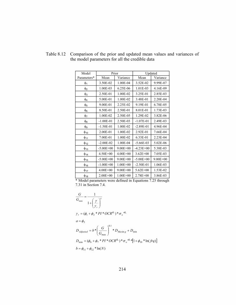
214
Table 8.12 Comparison of the prior and updated mean values and variances of the model parameters for all the credible data
Mean Variance Mean Varianceφ1 3.50E-02 1.00E-04 3.52E-02 9.99E-07φ2 1.00E-03 6.25E-06 1.01E-03 4.16E-09φ3 2.50E-01 1.00E-02 3.25E-01 2.85E-03φ4 5.00E-01 1.00E-02 3.48E-01 2.20E-04φ5 9.00E-01 2.25E-02 9.19E-01 6.78E-05φ6 8.50E-01 2.50E-01 8.01E-01 1.73E-03φ7 1.00E-02 2.50E-05 1.29E-02 3.82E-06φ8 -1.00E-01 2.50E-03 -1.07E-01 2.49E-03φ9 -1.50E-01 1.00E-02 -2.89E-01 4.96E-04φ10 2.00E-01 1.00E-02 2.92E-01 7.66E-04φ11 7.00E-01 1.00E-02 6.33E-01 2.23E-04φ12 -2.00E-02 1.00E-04 -5.66E-03 5.02E-06φ13 -5.00E+00 9.00E+00 -4.23E+00 5.38E-03φ14 4.50E+00 4.00E+00 3.62E+00 7.05E-03φ15 -5.00E+00 9.00E+00 -5.00E+00 9.00E+00φ16 -1.00E+00 1.00E+00 -2.50E-01 1.06E-03φ17 4.00E+00 9.00E+00 5.62E+00 1.53E-02φ18 2.00E+00 1.00E+00 2.78E+00 3.86E-03
Prior UpdatedModel Parameters*
* Model parameters were defined in Equations 7.25 through 7.31 in Section 7.4.
a
r
GG
+
=
γγ1
1
max
43 '*)**( 21φφ σφφγ or OCRPI+=
5φ=a
minsin
1.0
max** DD
GGbD gMaAdjusted +
=
[ ])ln(*1*'*)**( 1076min98 frqOCRPID o φσφφ φφ ++=
)ln(*1211 Nb φφ +=

215
1.2
1.0
0.8
0.6
0.4
0.2
0.0
Pred
icte
d N
orm
aliz
ed M
odul
us
1.21.00.80.60.40.20.0
Measured Normalized Modulus
Figure 8.26 Comparisons of the measured and predicted values of normalized modulus for all credible data

216
25
20
15
10
5
0
Pred
icte
d M
ater
ial D
ampi
ng
2520151050
Measured Material Damping
Figure 8.27 Comparisons of the measured and predicted values of material damping for all credible data
217
Table 8.13 shows the covariance structure of the model parameters. This
information can be utilized in calculating model uncertainty associated with the
normalized modulus reduction and material damping curves estimated based on
this model as discussed in Chapter Eleven. Since the model is calibrated to a
rather large database, most of the uncertainty however results from the variability
within the database modeled using parameters φ13 through φ18 (Section 7.4.2).
8.4 SUMMARY
In order to study the effect of soil type and geology, the data was first
analyzed in several subsets according to soil group (“clean” sands, sands with
high fines content, silts and clays) and geographic location (Northern California,
Southern California, South Carolina and Lotung, Taiwan).
Four specimens from South Carolina (specimens UT-39-G, UT-39-M,
UT-39-O, and UT-39-S) were removed from the database following the analysis
because the resonant column results did not follow the general trends reported in
the literature and observed during the course of this study. The torsional shear
results for these specimens did follow the general trends but were not of sufficient
strain range to be included. At this point, the analyses affected by the change in
the content of the database were repeated and the rest of the analyses were carried
out without utilizing the data associated with these four specimens.
The test results of all specimens from each soil group (regardless of
geographic location) were also analyzed in order to study the effect of soil type on
model parameters.
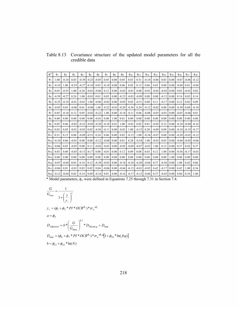
218
Table 8.13 Covariance structure of the updated model parameters for all the credible data
φi* φ1 φ2 φ3 φ4 φ5 φ6 φ7 φ8 φ9 φ10 φ11 φ12 φ13 φ14 φ15 φ16 φ17 φ18
φ1 1.00 -0.10 0.03 -0.39 -0.25 -0.05 0.05 0.00 0.05 0.03 0.51 -0.10 -0.06 0.03 0.00 -0.07 -0.06 -0.12
φ2 -0.10 1.00 -0.55 -0.27 -0.10 0.03 -0.18 0.00 0.06 0.05 0.15 0.06 0.03 0.00 0.00 -0.04 0.01 -0.04
φ3 0.03 -0.55 1.00 0.24 -0.01 -0.06 0.12 0.00 -0.02 -0.01 0.00 -0.01 -0.03 -0.03 0.00 0.03 -0.01 0.02
φ4 -0.39 -0.27 0.24 1.00 -0.01 0.01 0.05 0.00 -0.23 -0.03 -0.09 0.08 0.00 -0.13 0.00 0.14 0.03 0.14
φ5 -0.25 -0.10 -0.01 -0.01 1.00 -0.06 -0.02 0.00 -0.05 0.02 -0.51 0.00 0.11 -0.17 0.00 0.12 0.02 0.09
φ6 -0.05 0.03 -0.06 0.01 -0.06 1.00 -0.22 -0.01 -0.20 -0.56 0.24 -0.12 -0.02 0.08 0.00 -0.30 0.04 -0.10
φ7 0.05 -0.18 0.12 0.05 -0.02 -0.22 1.00 0.00 -0.18 -0.11 0.06 -0.08 -0.03 -0.01 0.00 -0.03 -0.06 0.01
φ8 0.00 0.00 0.00 0.00 0.00 -0.01 0.00 1.00 0.01 0.00 0.00 0.00 0.00 0.00 0.00 0.00 0.00 0.00
φ9 0.05 0.06 -0.02 -0.23 -0.05 -0.20 -0.18 0.01 1.00 -0.01 0.02 0.01 -0.05 0.12 0.00 -0.18 -0.04 -0.16
φ10 0.03 0.05 -0.01 -0.03 0.02 -0.56 -0.11 0.00 -0.01 1.00 -0.15 0.28 -0.09 0.09 0.00 -0.10 -0.15 -0.17
φ11 0.51 0.15 0.00 -0.09 -0.51 0.24 0.06 0.00 0.02 -0.15 1.00 -0.54 -0.07 0.08 0.00 -0.20 -0.01 -0.12
φ12 -0.10 0.06 -0.01 0.08 0.00 -0.12 -0.08 0.00 0.01 0.28 -0.54 1.00 -0.03 0.03 0.00 -0.04 -0.05 -0.06
φ13 -0.06 0.03 -0.03 0.00 0.11 -0.02 -0.03 0.00 -0.05 -0.09 -0.07 -0.03 1.00 0.12 0.00 0.37 0.42 0.37
φ14 0.03 0.00 -0.03 -0.13 -0.17 0.08 -0.01 0.00 0.12 0.09 0.08 0.03 0.12 1.00 0.00 -0.56 -0.17 -0.65
φ15 0.00 0.00 0.00 0.00 0.00 0.00 0.00 0.00 0.00 0.00 0.00 0.00 0.00 0.00 1.00 0.00 0.00 0.00
φ16 -0.07 -0.04 0.03 0.14 0.12 -0.30 -0.03 0.00 -0.18 -0.10 -0.20 -0.04 0.37 -0.56 0.00 1.00 0.42 0.86
φ17 -0.06 0.01 -0.01 0.03 0.02 0.04 -0.06 0.00 -0.04 -0.15 -0.01 -0.05 0.42 -0.17 0.00 0.42 1.00 0.34
φ18 -0.12 -0.04 0.02 0.14 0.09 -0.10 0.01 0.00 -0.16 -0.17 -0.12 -0.06 0.37 -0.65 0.00 0.86 0.34 1.00 * Model parameters, φi, were defined in Equations 7.25 through 7.31 in Section 7.4.
a
r
GG
+
=
γγ1
1
max
43 '*)**( 21φφ σφφγ or OCRPI+=
5φ=a
minsin
1.0
max** DD
GGbD gMaAdjusted +
=
[ ])ln(*1*'*)**( 1076min98 frqOCRPID o φσφφ φφ ++=
)ln(*1211 Nb φφ +=

219
After concluding that the effects of geology (analyzed through geographic
location) and fines content (analyzed through soil groups) on the model
parameters were not very pronounced based on the analysis of subsets of the
database, all credible data (within the updated database) were analyzed as one
complete data set to calibrate the model. Calculation of mean normalized modulus
reduction and material damping curves and handling uncertainty associated with
these curves are discussed in the following chapters.

220
CHAPTER 9
PREDICTING NONLINEAR SOIL BEHAVIOR USING THE
CALIBRATED MODEL
9.1 INTRODUCTION
Proposed equations discussed in Section 7.4 have been calibrated using all
credible data in Section 8.3. The updated mean values of the model parameters
presented in Table 8.12 can be used to estimate normalized modulus reduction
and material damping curves for a broad range of soil types and loading
conditions.
Since the predictions are based on the model calibrated using all credible
data, the effects of a number of parameters regarding soil type (geology, fines
content, particle size, particle stiffness, etc.) are ignored in this model. The only
indicator of soil characteristics utilized in the estimation of nonlinear behavior is
plasticity index, PI.
In this chapter, estimation of nonlinear curves for a given soil plasticity
and loading condition is presented. Additionally, general trends based on these
estimated curves and their consistency with previous studies are discussed.

221
9.2 CALCULATION OF REFERENCE STRAIN, CURVATURE COEFFICIENT, SMALL-STRAIN MATERIAL DAMPING RATIO AND THE SCALING COEFFICIENT
The equations presented in Section 7.4.1 can be utilized to calculate
reference strain, curvature coefficient, small-strain material damping ratio and the
scaling coefficient by replacing parameters (φi) with their updated mean values
presented in Table 8.12 as follows: 43 '*)**( 21
φφ σφφγ or OCRPI+= (9.1a)
5φ=a (9.1b)
[ ])ln(*1*'*)**( 1076min98 frqOCRPID o φσφφ φφ ++= (9.1c)
)ln(*1211 Nb φφ += (9.1d)
where: σo’ = mean effective confining pressure (atm),
PI = soil plasticity (%),
OCR = overconsolidation ratio,
frq = loading frequency,
N = number of loading cycles,
φ1 = 0.0352,
φ2 = 0.0010,
φ3 = 0.3246,
φ4 = 0.3483,
φ5 = 0.9190,
φ6 = 0.8005,
φ7 = 0.0129,
φ8 = -0.1069,

222
φ9 = -0.2889,
φ10 = 0.2919,
φ11 = 0.6329, and
φ12 = -0.0057.
In this way, the relationship between the four model parameters (reference
strain, curvature coefficient, small-strain material damping ratio and the scaling
coefficient) discussed in Chapter Six, and soil plasticity and loading conditions
can be established based on statistical analysis of the database. These
relationships are also presented in a graphical form to assist the reader in
understanding the model characteristics and in utilizing the model.
Figure 9.1 shows a graphical tool that can be used to estimate reference
strain for given values of PI, OCR and in-situ mean effective stress. An example
solution is presented utilizing a clayey soil with PI = 60 % and moderate
overconsolidation (OCR = 4) subjected to 4 atm in-situ mean effective stress.
Starting with the PI and OCR of the soil, reference strain of the material is
estimated as if it were subjected to 1 atm confining pressure. This value is then
adjusted for the effect of confining pressure in the graphical solution.
Figure 9.2 shows the graphical solution for the scaling coefficient, b.
Calculation of the value for ten cycles of loading is presented as an example in
this figure.

223
100 80 60 40 20 0
Plasticity Index, %
OCR = 1
OCR = 4
OCR = 16
0.30
0.25
0.20
0.15
0.10
0.05
0.00
Ref
eren
ce S
train
at 1
atm
, %
0.01 0.1 1
Reference Strain, %
σ o' =
1 a
tm
σ o' =
4 a
tm
σ o' =
16
atm
σ o' =
0.2
5 at
m
Figure 9.1 Estimation of reference strain for given values of PI, OCR and in-situ mean effective stress
0.64
0.63
0.62
0.61
0.60
0.59
0.58
Scal
ing
Coe
ffici
ent,
b
1 10 100 1000
Number of Loading Cycles
Figure 9.2 Estimation of scaling coefficient for a given value of number of loading cycles
224
Calculation of the small-strain material damping ratio is presented in
graphical form in Figure 9.3. As in the case of reference strain, small-strain
material damping ratio can be estimated graphically for given values of PI, OCR
in-situ mean effective stress and loading frequency. An example solution is
presented utilizing a clayey soil with PI = 60 % and moderate overconsolidation
(OCR = 4) subjected to 4 atm in-situ mean effective stress loaded at 10 Hz.
Starting with the PI and OCR of the soil, the small-strain material damping ratio
is estimated as if it were subjected to 1 atm confining pressure loaded at 1 Hz.
This value is adjusted for the effect of confining pressure and then for loading
frequency in the graphical solution.
9.3 ESTIMATION OF NORMALIZED MODULUS REDUCTION AND MATERIAL DAMPING CURVES
Once the four model parameters (reference strain, curvature coefficient,
small-strain material damping ratio, and scaling coefficient) are calculated for the
soil plasticity and loading conditions, the equations presented in Chapter Six can
be utilized to estimate the normalized modulus reduction and material damping
curves as follows:
a
r
GG
+
=
γγ1
1
max
(9.2a)
minsin
1.0
max** DD
GGbD gMaAdjusted +
= (9.2b)

225
100 80 60 40 20 0
Plasticity Index, %
OCR = 1
OCR = 4
OCR = 16
Dm
in a
t 1 a
tm a
nd a
t 1 H
z, %
1.0
1.2
1.4
1.6
1.8
2.0
2.2
0.80.1 1 10
Dmin at 1 Hz, %
σ o' =
1 a
tmσ o
' = 4
atm
σ o' =
16
atm
σ o' =
0.2
5 at
m
0.1
1
10
Dm
in, %
f = 10 Hz
f = 1 Hz
f = 100 Hz
Figure 9.3 Estimation of small-strain material damping ratio for given values of PI, OCR, in-situ mean effective stress and loading frequency

226
where:maxGG = normalized shear modulus,
γ = shearing strain (%),
γr = reference strain (%),
a = curvature coefficient,
Dmin = small-strain material damping ratio (%),
b = scaling coefficient,
DAdjusted = scaled and capped material damping (%), 3
0.1,sin32
0.1,sin20.1,sin1sin === ++= agMaagMaagMagMa DcDcDcD (%),
−
+
+−
Π== 2
ln4100
20.1,sin
r
r
rr
agMaD
γγγ
γγγ
γγ (%),
0.2523 + 1.8618a + -1.1143a21 =c ,
0.0095 - 0.0710a - 0.0805a 22 =c , and
0.0003 + 0.0002a + 0.0005a- 23 =c .
Figure 9.4 shows the normalized modulus reduction and material damping
curves for the soil type and loading conditions presented in Section 9.2, a clayey
soil with PI = 60 % and moderate overconsolidation (OCR = 4) subjected to 4 atm
in-situ mean effective stress and ten cycles of loading at 10 Hz.

227
1.2
1.0
0.8
0.6
0.4
0.2
0.0
G/Gmax G/Gmax Predictionγ r = 0.212 %a = 0.92
(a)
25
20
15
10
5
0
D, %
0.0001 0.001 0.01 0.1 1
Shearing Strain, γ ,%
Material Damping Predictionγ r = 0.212 %a = 0.92Dmin = 1.65b = 0.62
(b)
Figure 9.4 Estimated (a) normalized modulus reduction and (b) material damping curves for the soil type and loading conditions discussed in Section 9.2

228
It is important to note that the nonlinear behavior predicted by the model
is based on data collected over shearing strain amplitudes ranging from 1x10⁻⁵ %
to less than 1 %. As a result, extrapolation of the curves to higher strain
amplitudes is not recommended. Also, predicted material damping ratios at strain
amplitudes over 10 % will decrease to smaller values because of the damping
adjustment that introduces a cap on material damping. Consequently, the model
should never be utilized in modeling soil behavior at such high strain levels unless
the results are verified by additional tests performed at high strain amplitudes.
9.4 EFFECT OF OVERCONSOLIDATION RATIO, LOADING FREQUENCY AND NUMBER OF LOADING CYCLES ON NONLINEAR SOIL BEHAVIOR
The effects of overconsolidation ratio, loading frequency and number of
loading cycles have been included in the model calibrated in Chapter Eight. The
results indicate that the effects of these variables on dynamic soil behavior are not
pronounced for the competent soils (that do not exhibit large volume change when
sheared at strains less than 1 %) investigated in this study.
Figure 9.5 presents the effect of overconsolidation ratio on nonlinear soil
behavior predicted by the calibrated model. Increasing overconsolidation ratio is
observed to result in a slight shift of the normalized modulus reduction and
material damping curves to higher strain amplitudes, along with a slight decrease
in small-strain material damping ratio. This effect is more pronounced for high
plasticity materials. These trends are consistent with those proposed by Hardin
and Drnevich (1972b).

229
1.2
1.0
0.8
0.6
0.4
0.2
0.0
G/Gmax
G/Gmax Prediction( σo' = 1 atm, PI = 15 %, N = 10 cycles, f = 1 Hz )
OCR = 1OCR = 4OCR = 16
(a)
25
20
15
10
5
0
D, %
0.0001 0.001 0.01 0.1 1
Shearing Strain, γ ,%
Material Damping Prediction( σo' = 1 atm, PI = 15 %, N = 10 cycles, f = 1 Hz )
OCR = 1OCR = 4OCR = 16
(b)
Figure 9.5 Effect of overconsolidation ratio on (a) normalized modulus reduction and (b) material damping curves predicted by the calibrated model

230
In Figures 9.6 and 9.7, the effects of loading frequency and number of
loading cycles are shown. As discussed in Section 8.3, the model has been
formulated ignoring the effect of these two variables on the normalized modulus
reduction curve based on general trends observed during the course of this study.
Figure 9.6a and 9.7a are presented to clarify this issue.
Figure 9.6b presents the effect of loading frequency on the material
damping curve predicted by the calibrated model. An increase in small-strain
material damping ratio with increasing loading frequency is observed in this
figure. This effect is consistent with the trends reported in Stokoe et al. (1999).
In Figure 9.7b, the effect of number of loading cycles on the material
damping curve is presented. Increasing number of cycles results in a slight
decrease in the scaling coefficient causing a slight decrease of material damping
ratio at high strains. This general trend is also consistent with the trends reported
in Hardin and Drnevich (1972b) and Stokoe et al. (1999).
The database utilized to calibrate the four-parameter model consists of the
results of the first and tenth cycles of torsional shear tests performed at 1 Hz and
resonant column tests performed at the resonant frequency of the specimen that is
typically on the order of around 100 Hz. During resonant column testing, the
specimen is cycled about 1000 times. Thus, the combined effect of loading
frequency and number of loading cycles is presented in Figure 9.8 showing the
predicted difference between hypothetical test results.

231
1.2
1.0
0.8
0.6
0.4
0.2
0.0
G/Gmax
G/Gmax Prediction( σo' = 1 atm, PI = 15 %, N = 10 cycles, OCR = 1 )
f = 1 Hzf = 10 Hzf = 100 Hz
(a)
25
20
15
10
5
0
D, %
0.0001 0.001 0.01 0.1 1
Shearing Strain, γ ,%
Material Damping Prediction( σo' = 1 atm, PI = 15 %, N = 10 cycles, OCR = 1 )
f = 1 Hzf = 10 Hzf = 100 Hz
(b)
Figure 9.6 Effect of loading frequency on (a) normalized modulus reduction and (b) material damping curves predicted by the calibrated model
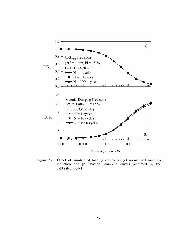
232
1.2
1.0
0.8
0.6
0.4
0.2
0.0
G/Gmax
G/Gmax Prediction( σo' = 1 atm, PI = 15 %, f = 1 Hz, OCR =1 )
N = 1 cyclesN = 10 cyclesN = 1000 cycles
(a)
25
20
15
10
5
0
D, %
0.0001 0.001 0.01 0.1 1
Shearing Strain, γ ,%
Material Damping Prediction( σo' = 1 atm, PI = 15 %, f = 1 Hz, OCR =1 )
N = 1 cyclesN = 10 cyclesN = 1000 cycles
(b)
Figure 9.7 Effect of number of loading cycles on (a) normalized modulus reduction and (b) material damping curves predicted by the calibrated model
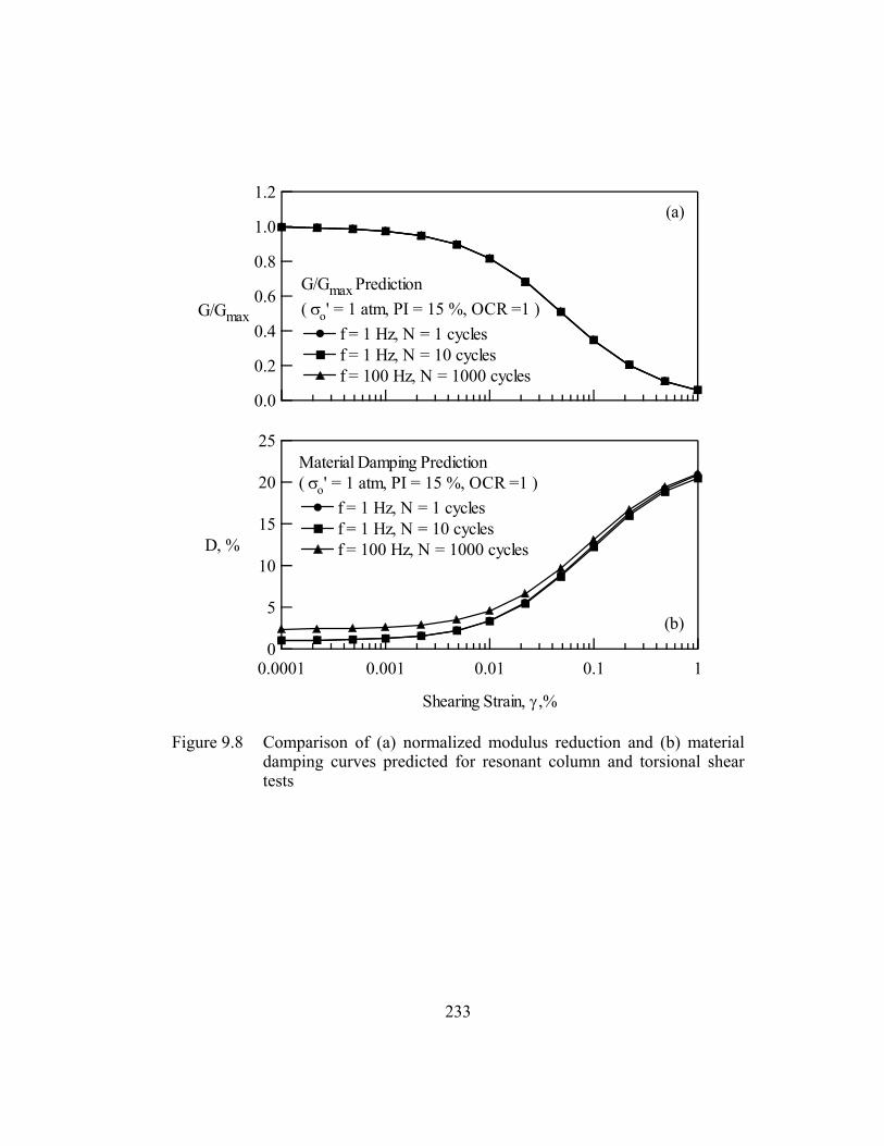
233
1.2
1.0
0.8
0.6
0.4
0.2
0.0
G/Gmax
G/Gmax Prediction( σo' = 1 atm, PI = 15 %, OCR =1 )
f = 1 Hz, N = 1 cyclesf = 1 Hz, N = 10 cyclesf = 100 Hz, N = 1000 cycles
(a)
25
20
15
10
5
0
D, %
0.0001 0.001 0.01 0.1 1
Shearing Strain, γ ,%
Material Damping Prediction( σo' = 1 atm, PI = 15 %, OCR =1 )
f = 1 Hz, N = 1 cyclesf = 1 Hz, N = 10 cyclesf = 100 Hz, N = 1000 cycles
(b)
Figure 9.8 Comparison of (a) normalized modulus reduction and (b) material damping curves predicted for resonant column and torsional shear tests
234
9.5 EFFECT OF CONFINING PRESSURE ON NONLINEAR SOIL BEHAVIOR
The effect of confining pressure on normalized modulus reduction and
material damping curves predicted by the calibrated four-parameter model is
presented in Figure 9.9. The model shows the shift of normalized modulus
reduction and material damping curves to higher strain amplitudes with increasing
confining pressure along with a simultaneous decrease in small-strain material
damping ratio.
In Figure 9.10, the empirical curves proposed by Seed et al. (1986) are
presented. The comparison of the normalized modulus reduction curves predicted
by the calibrated model (Figure 9.9a) and the empirical curves proposed by Seed
et al. (1986) (Figure 9.10a) are presented in Figure 9.11a. The fact that the
nonlinear curves analyzed in Seed et al. (1986) were collected at low confining
pressures is supported by the close agreement between the mean Seed et al.
(1986) curve and the calibrated model curve for 1 atm. However, the comparison
of the material damping curves in Figure 9.11b shows that the material damping
values proposed by Seed et al. (1986) are higher than those encountered in the
course of this study. The discrepancy is believed to result from accuracy problems
in material damping measurements arising from the use of older generation cyclic
triaxial equipment employed in previous studies.

235
1.2
1.0
0.8
0.6
0.4
0.2
0.0
G/Gmax G/Gmax Prediction( PI = 0 %, N = 10 cycles, f = 1 Hz, OCR = 1 )
(a)
25
20
15
10
5
0
D, %
0.0001 0.001 0.01 0.1 1
Shearing Strain, γ ,%
Material Damping Predictionσo' = 0.25 atmσo' = 1 atmσo' = 4 atmσo' = 16 atm
(b)
Figure 9.9 Effect of confining pressure on (a) normalized modulus reduction and (b) material damping curves predicted by the calibrated model
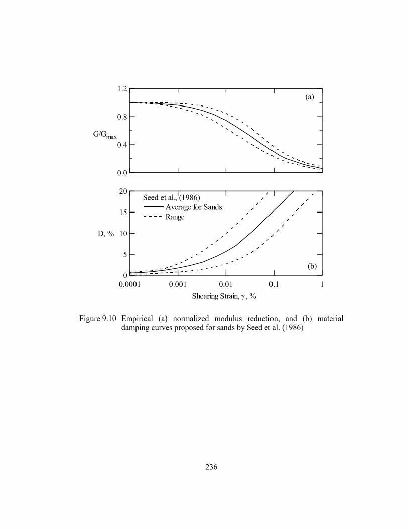
236
1.2
0.8
0.4
0.0
G/Gmax
(a)
20
15
10
5
0
D, %
0.0001 0.001 0.01 0.1 1Shearing Strain, γ , %
Seed et al., (1986)Average for SandsRange
(b)
Figure 9.10 Empirical (a) normalized modulus reduction, and (b) material damping curves proposed for sands by Seed et al. (1986)

237
1.2
1.0
0.8
0.6
0.4
0.2
0.0
G/Gmax
G/Gmax Prediction( PI = 0 %, N = 10 cycles, f = 1 Hz, OCR = 1 )
(a)
Seed et al. (1986)
25
20
15
10
5
0
D, %
0.0001 0.001 0.01 0.1 1
Shearing Strain, γ ,%
Material Damping Predictionσo' = 0.25 atmσo' = 1 atmσo' = 4 atmσo' = 16 atm
(b)
Figure 9.11 Comparison of the effect of confining pressure on nonlinear soil behavior of sand (PI = 0 %) predicted by the calibrated model and empirical curves proposed for sands by Seed et al. (1986)
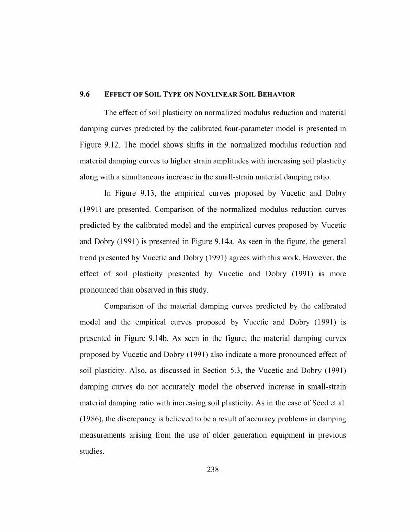
238
9.6 EFFECT OF SOIL TYPE ON NONLINEAR SOIL BEHAVIOR
The effect of soil plasticity on normalized modulus reduction and material
damping curves predicted by the calibrated four-parameter model is presented in
Figure 9.12. The model shows shifts in the normalized modulus reduction and
material damping curves to higher strain amplitudes with increasing soil plasticity
along with a simultaneous increase in the small-strain material damping ratio.
In Figure 9.13, the empirical curves proposed by Vucetic and Dobry
(1991) are presented. Comparison of the normalized modulus reduction curves
predicted by the calibrated model and the empirical curves proposed by Vucetic
and Dobry (1991) is presented in Figure 9.14a. As seen in the figure, the general
trend presented by Vucetic and Dobry (1991) agrees with this work. However, the
effect of soil plasticity presented by Vucetic and Dobry (1991) is more
pronounced than observed in this study.
Comparison of the material damping curves predicted by the calibrated
model and the empirical curves proposed by Vucetic and Dobry (1991) is
presented in Figure 9.14b. As seen in the figure, the material damping curves
proposed by Vucetic and Dobry (1991) also indicate a more pronounced effect of
soil plasticity. Also, as discussed in Section 5.3, the Vucetic and Dobry (1991)
damping curves do not accurately model the observed increase in small-strain
material damping ratio with increasing soil plasticity. As in the case of Seed et al.
(1986), the discrepancy is believed to be a result of accuracy problems in damping
measurements arising from the use of older generation equipment in previous
studies.
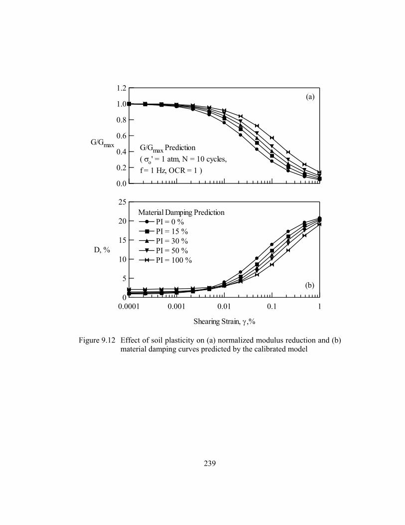
239
1.2
1.0
0.8
0.6
0.4
0.2
0.0
G/Gmax G/Gmax Prediction( σo' = 1 atm, N = 10 cycles, f = 1 Hz, OCR = 1 )
(a)
25
20
15
10
5
0
D, %
0.0001 0.001 0.01 0.1 1
Shearing Strain, γ ,%
Material Damping PredictionPI = 0 %PI = 15 %PI = 30 %PI = 50 %PI = 100 %
(b)
Figure 9.12 Effect of soil plasticity on (a) normalized modulus reduction and (b) material damping curves predicted by the calibrated model
240
1.2
0.8
0.4
0.0
G/Gmax
(a)
20
15
10
5
0
D, %
0.0001 0.001 0.01 0.1 1Shearing Strain, γ , %
Vucetic and Dobry (1991)Non-PlasticPI = 15 %PI = 30 %PI = 50 %PI = 100 %PI = 200 %
(b)
Figure 9.13 Empirical (a) normalized modulus reduction, and (b) material damping curves proposed by Vucetic and Dobry (1991)

241
1.2
1.0
0.8
0.6
0.4
0.2
0.0
G/Gmax
G/Gmax Prediction( σo' = 1 atm, N = 10 cycles, f = 1 Hz, OCR = 1 )
Vucetic and Dobry (1991)
(a)
25
20
15
10
5
0
D, %
0.0001 0.001 0.01 0.1 1
Shearing Strain, γ ,%
Material Damping PredictionPI = 0 %PI = 15 %PI = 30 %PI = 50 %PI = 100 %
(b)
Figure 9.14 Comparison of the effect of soil plasticity on nonlinear soil behavior predicted by the calibrated model and empirical curves proposed by Vucetic and Dobry (1991)
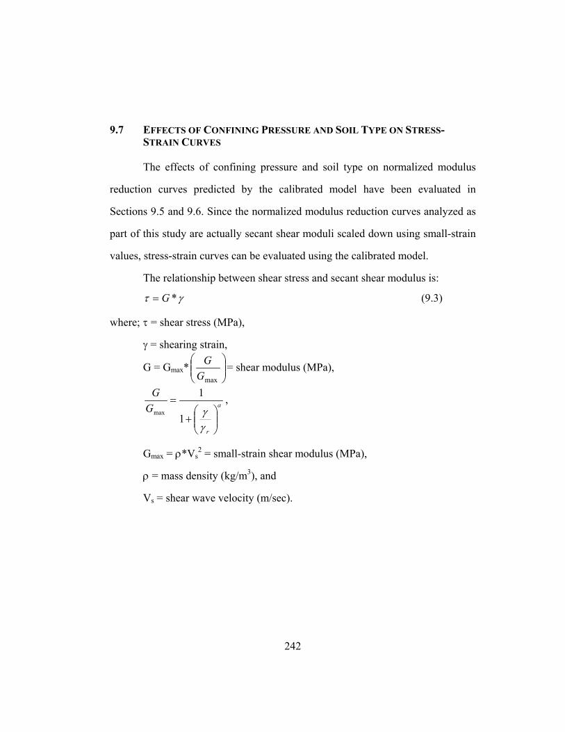
242
9.7 EFFECTS OF CONFINING PRESSURE AND SOIL TYPE ON STRESS-STRAIN CURVES
The effects of confining pressure and soil type on normalized modulus
reduction curves predicted by the calibrated model have been evaluated in
Sections 9.5 and 9.6. Since the normalized modulus reduction curves analyzed as
part of this study are actually secant shear moduli scaled down using small-strain
values, stress-strain curves can be evaluated using the calibrated model.
The relationship between shear stress and secant shear modulus is:
γτ *G= (9.3)
where; τ = shear stress (MPa),
γ = shearing strain,
G = Gmax*
maxGG = shear modulus (MPa),
a
r
GG
+
=
γγ1
1
max
,
Gmax = ρ*Vs2 = small-strain shear modulus (MPa),
ρ = mass density (kg/m3), and
Vs = shear wave velocity (m/sec).

243
Equation 9.3 illustrates that, in order to estimate stress-strain curves based on the
four-parameter model, the impact of confining pressure and soil type on shear
wave velocity has to be evaluated. The relationship between these parameters and
in-situ shear wave velocity measurements can be assessed utilizing the same
database that was used to calibrate the four-parameter model. Eighty seven of the
specimens within the database were sampled from sites where in-situ shear wave
velocity measurements had been performed (Chiara, 2001). A least-squares fit to
part of the data suggests the following relationship:
PIV os *44.2'*300 27.0 −= σ (9.4)
where; σo’ = mean effective confining pressure (atm), and
PI = plasticity index (%).
The comparison of the predicted values of shear wave velocity and
measured values is presented in Figure 9.15 so that the reader can evaluate the
quality of the fit. Equation 9.4 is not part of the calibrated model recommended
for evaluating dynamic soil behavior and is utilized only as a starting point to
generate stress-strain curves presented in this section.
The effects of confining pressure and soil type on stress-strain curves
predicted using the calibrated four-parameter model are presented in Figures 9.16
and 9.17, respectively. Figures 9.16a and 9.17a show the predictions for shearing
strains up to 1 %. Figures 9.16b and 9.17b show the predictions for shearing
strains up to 0.01 % so that the characteristics of the curves at smaller strains can
be presented to the reader.

244
1000
800
600
400
200
0
Pred
icte
d Sh
ear W
ave
Vel
ocity
, m/se
c
10008006004002000
Measured Shear Wave Velocity, m/sec
Figure 9.15 Comparison of the measured in-situ shear wave velocities and values predicted using Equation 9.4
The model successfully predicts the increase in shear strength with
increasing confining pressure as shown in Figure 9.16. Figure 9.17 shows a
comparison of predicted stress-strain curves for soils with different plasticities.
Figure 9.18 shows part of the data in Figure 9.17 in an effort to compare the
behavior of a sand (PI = 0 %) and a moderate plasticity clay (PI = 30 %). It is
important to note the similarity between this figure and Figure 5.1b from Hardin
and Drnevich (1972b).

245
300
250
200
150
100
50
0
τ, kPa
1.00.80.60.40.20.0
Shearing Strain, γ ,%
σo' = 0.25 atmσo' = 1 atmσo' = 4 atm
(a)
10
8
6
4
2
0
τ, kPa
0.0100.0080.0060.0040.0020.000
Shearing Strain, γ ,%
σo' = 0.25 atmσo' = 1 atmσo' = 4 atm
(b)
Figure 9.16 Effect of confining pressure on stress-strain curve predicted by the calibrated model for shearing strains ranging (a) from γ = 0 to 1 % and (b) from γ = 0 to 0.01 %

246
100
80
60
40
20
0
τ, kPa
1.00.80.60.40.20.0
Shearing Strain, γ ,%
PI = 0 %PI = 15 %PI = 30 %PI = 50 %
(a)
10
8
6
4
2
0
τ, kPa
0.0100.0080.0060.0040.0020.000
Shearing Strain, γ ,%
PI = 0 %PI = 15 %PI = 30 %PI = 50 %
(b)
Figure 9.17 Effect of soil plasticity on stress-strain curve predicted by the calibrated model for shearing strains ranging (a) from γ = 0 to 1 % and (b) from γ = 0 to 0.01 %

247
100
80
60
40
20
0
τ, kPa
1.00.80.60.40.20.0
Shearing Strain, γ ,%
PI = 0 %PI = 30 %
(a)
10
8
6
4
2
0
τ, kPa
0.0100.0080.0060.0040.0020.000
Shearing Strain, γ ,%
PI = 0 %PI = 30 %
(b)
Figure 9.18 Comparison of the stress-strain curves of a sand and a moderate plasticity clay based on the calibrated model for shearing strains ranging (a) from γ = 0 to 1 % and (b) from γ = 0 to 0.01 %

248
9.8 SUMMARY
In this chapter, equations for the calibrated model are presented along with
graphical solutions that can be utilized in predicting normalized modulus
reduction and material damping curves for a given soil type and a given loading
condition.
The general trends of the predicted curves are briefly discussed. The
results indicate that soil plasticity and mean effective confining pressure are the
two most important parameters that control nonlinear behavior of “competent”
soils strained up to γ = 1 %. The comparison of the predicted curves with those
presented in the literature indicates a general agreement with the trends proposed
by other researchers. However, this comparison also highlights discrepancies in
material damping measurements resulting from the limitations of older generation
testing equipment utilized in previous studies.
Since stress-strain curves are related to normalized shear modulus curves,
a brief discussion regarding the predicted stress-strain curves based on the
calibrated model is also presented herein in an effort to bridge the gap between
traditional geotechnical engineering and soil dynamics. The findings indicate that
the results of dynamic tests can also be utilized in the traditional geotechnical
engineering applications that require modeling soil behavior at working strains.

249
CHAPTER 10
RECOMMENDED NORMALIZED MODULUS REDUCTION
AND MATERIAL DAMPING CURVES
10.1 INTRODUCTION
Mean values of the normalized shear modulus and the material damping
ratio (predicted by the calibrated model) at strain amplitudes ranging from 1x10⁻⁵
% to 1 % are presented in this chapter. As discussed in Chapter Nine, the mean
values of model parameters can be utilized to construct normalized modulus
reduction and material damping curves for different soil types and loading
conditions. However, the reader must use caution when a soil type or loading
condition not represented in the database is to be evaluated with these equations.
Since the impact of overconsolidation ratio is relatively small and ten
cycles at 1 Hz loading frequency closely represents the characteristics of
earthquake shaking, these parameters are fixed for the recommended curves. In
this chapter, recommended normalized modulus reduction and material damping
curves are presented for soils with a broad range of plasticities confined at a broad
range of mean effective stresses.
These curves are presented from two different perspectives so that the
reader can interpolate the data for different values of soil plasticity and confining
pressure. If the reader has to extrapolate for soil plasticities and confining
pressures not represented in the database, use of caution is suggested.

250
10.2 EFFECT OF PI AT A GIVEN MEAN EFFECTIVE STRESS
Figures 10.1 through 10.4 show the effect of PI on nonlinear soil behavior
at 0.25, 1.0, 4.0 and 16 atm, respectively. These normalized modulus and material
damping curves are presented so that the reader can interpolate these relationships
for soils with different plasticities. Also, these curves are tabulated in Tables 10.1
through 10.8. The figures and tables are organized so that the G/Gmax – log γ and
D – log γ curves are followed on the next page by the associated tables.
10.3 EFFECT OF MEAN EFFECTIVE STRESS ON A SOIL WITH GIVEN PLASTICITY
Figures 10.5 through 10.9 show the effect of mean effective stress on
nonlinear behavior of soils with 0, 15, 30, 50 and 100 % plasticity, respectively.
These normalized modulus and material damping curves are presented so that the
reader can interpolate these relationships for soil layers at different depths
confined under different mean effective stresses. Also, these curves are tabulated
in Tables 10.9 through 10.18. The figures and tables are organized so that the
G/Gmax – log γ and D – log γ curves are followed on the next page by the
associated tables.
10.4 IMPACT OF UTILIZING THE RECOMMENDED CURVES ON EARTHQUAKE RESPONSE PREDICTIONS OF DEEP SOIL SITES
The impact of utilizing the recommended curves when assigning nonlinear
soil properties in site response analyses of deep (>50 m) soil sites is discussed in
this section. This point is addressed because site response analyses are often
performed using average, pressure-independent generic curves.
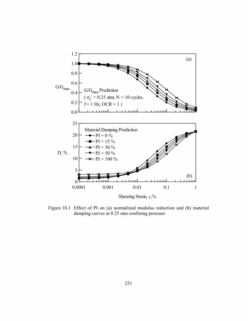
251
1.2
1.0
0.8
0.6
0.4
0.2
0.0
G/Gmax G/Gmax Prediction( σo' = 0.25 atm, N = 10 cycles, f = 1 Hz, OCR = 1 )
(a)
25
20
15
10
5
0
D, %
0.0001 0.001 0.01 0.1 1
Shearing Strain, γ ,%
Material Damping PredictionPI = 0 %PI = 15 %PI = 30 %PI = 50 %PI = 100 %
(b)
Figure 10.1 Effect of PI on (a) normalized modulus reduction and (b) material damping curves at 0.25 atm confining pressure

252
Table 10.1 Effect of PI on normalized modulus reduction curve: σo’ = 0.25 atm
Shearing Strain (%) PI = 0 % PI = 15 % PI = 30 % PI = 50 % PI = 100 %1.00E-05 0.999 0.999 1.000 1.000 1.0002.20E-05 0.998 0.999 0.999 0.999 1.0004.84E-05 0.996 0.997 0.998 0.998 0.9991.00E-04 0.993 0.995 0.996 0.997 0.9982.20E-04 0.986 0.990 0.992 0.994 0.9964.84E-04 0.971 0.979 0.983 0.987 0.9911.00E-03 0.944 0.959 0.968 0.975 0.9832.20E-03 0.891 0.919 0.936 0.949 0.9664.84E-03 0.799 0.847 0.876 0.900 0.9321.00E-02 0.671 0.739 0.783 0.822 0.8762.20E-02 0.497 0.579 0.637 0.692 0.7744.84E-02 0.324 0.400 0.459 0.521 0.6251.00E-01 0.197 0.255 0.303 0.358 0.4612.20E-01 0.107 0.142 0.174 0.213 0.2934.84E-01 0.055 0.074 0.093 0.116 0.1671.00E+00 0.029 0.040 0.050 0.063 0.093
Table 10.2 Effect of PI on material damping curve: σo’ = 0.25 atm
Shearing Strain (%) PI = 0 % PI = 15 % PI = 30 % PI = 50 % PI = 100 %1.00E-05 1.201 1.489 1.778 2.164 3.1292.20E-05 1.207 1.493 1.781 2.166 3.1314.84E-05 1.226 1.506 1.791 2.174 3.1361.00E-04 1.257 1.528 1.808 2.187 3.1442.20E-04 1.330 1.579 1.848 2.217 3.1634.84E-04 1.487 1.690 1.933 2.282 3.2041.00E-03 1.792 1.906 2.101 2.411 3.2862.20E-03 2.458 2.387 2.476 2.702 3.4724.84E-03 3.762 3.358 3.249 3.310 3.8681.00E-02 5.821 4.977 4.581 4.386 4.5932.20E-02 9.097 7.778 7.010 6.441 6.0704.84E-02 12.993 11.489 10.477 9.589 8.5791.00E-01 16.376 15.064 14.088 13.137 11.7982.20E-01 19.181 18.334 17.640 16.904 15.7164.84E-01 20.829 20.515 20.208 19.849 19.2131.00E+00 21.393 21.507 21.542 21.547 21.544

253
1.2
1.0
0.8
0.6
0.4
0.2
0.0
G/Gmax G/Gmax Prediction( σo' = 1 atm, N = 10 cycles, f = 1 Hz, OCR = 1 )
(a)
25
20
15
10
5
0
D, %
0.0001 0.001 0.01 0.1 1
Shearing Strain, γ ,%
Material Damping PredictionPI = 0 %PI = 15 %PI = 30 %PI = 50 %PI = 100 %
(b)
Figure 10.2 Effect of PI on (a) normalized modulus reduction and (b) material damping curves at 1.0 atm confining pressure
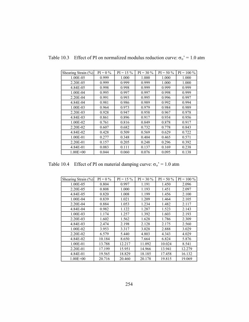
254
Table 10.3 Effect of PI on normalized modulus reduction curve: σo’ = 1.0 atm
Shearing Strain (%) PI = 0 % PI = 15 % PI = 30 % PI = 50 % PI = 100 %1.00E-05 0.999 1.000 1.000 1.000 1.0002.20E-05 0.999 0.999 0.999 1.000 1.0004.84E-05 0.998 0.998 0.999 0.999 0.9991.00E-04 0.995 0.997 0.997 0.998 0.9992.20E-04 0.991 0.993 0.995 0.996 0.9974.84E-04 0.981 0.986 0.989 0.992 0.9941.00E-03 0.964 0.973 0.979 0.984 0.9892.20E-03 0.928 0.947 0.958 0.967 0.9784.84E-03 0.861 0.896 0.917 0.934 0.9561.00E-02 0.761 0.816 0.849 0.878 0.9172.20E-02 0.607 0.682 0.732 0.778 0.8434.84E-02 0.428 0.509 0.569 0.629 0.7221.00E-01 0.277 0.348 0.404 0.465 0.5712.20E-01 0.157 0.205 0.248 0.296 0.3924.84E-01 0.083 0.111 0.137 0.169 0.2381.00E+00 0.044 0.060 0.076 0.095 0.138
Table 10.4 Effect of PI on material damping curve: σo’ = 1.0 atm
Shearing Strain (%) PI = 0 % PI = 15 % PI = 30 % PI = 50 % PI = 100 %1.00E-05 0.804 0.997 1.191 1.450 2.0962.20E-05 0.808 1.000 1.193 1.451 2.0974.84E-05 0.820 1.008 1.199 1.456 2.1001.00E-04 0.839 1.021 1.209 1.464 2.1052.20E-04 0.884 1.053 1.234 1.482 2.1174.84E-04 0.982 1.122 1.287 1.523 2.1431.00E-03 1.174 1.257 1.392 1.603 2.1932.20E-03 1.602 1.562 1.628 1.786 2.3094.84E-03 2.474 2.198 2.128 2.175 2.5601.00E-02 3.953 3.317 3.028 2.888 3.0292.20E-02 6.579 5.440 4.803 4.343 4.0294.84E-02 10.184 8.650 7.664 6.824 5.8761.00E-01 13.788 12.217 11.092 10.024 8.5412.20E-01 17.199 15.951 14.966 13.941 12.2794.84E-01 19.565 18.829 18.185 17.458 16.1321.00E+00 20.716 20.460 20.178 19.815 19.069

255
1.2
1.0
0.8
0.6
0.4
0.2
0.0
G/Gmax G/Gmax Prediction( σo' = 4 atm, N = 10 cycles, f = 1 Hz, OCR = 1 )
(a)
25
20
15
10
5
0
D, %
0.0001 0.001 0.01 0.1 1
Shearing Strain, γ ,%
Material Damping PredictionPI = 0 %PI = 15 %PI = 30 %PI = 50 %PI = 100 %
(b)
Figure 10.3 Effect of PI on (a) normalized modulus reduction and (b) material damping curves at 4.0 atm confining pressure

256
Table 10.5 Effect of PI on normalized modulus reduction curve: σo’ = 4.0 atm
Shearing Strain (%) PI = 0 % PI = 15 % PI = 30 % PI = 50 % PI = 100 %1.00E-05 1.000 1.000 1.000 1.000 1.0002.20E-05 0.999 1.000 1.000 1.000 1.0004.84E-05 0.998 0.999 0.999 0.999 1.0001.00E-04 0.997 0.998 0.998 0.999 0.9992.20E-04 0.994 0.996 0.997 0.997 0.9984.84E-04 0.988 0.991 0.993 0.995 0.9961.00E-03 0.976 0.983 0.986 0.989 0.9932.20E-03 0.952 0.965 0.972 0.978 0.9864.84E-03 0.906 0.931 0.945 0.956 0.9711.00E-02 0.832 0.873 0.898 0.918 0.9452.20E-02 0.706 0.770 0.810 0.845 0.8934.84E-02 0.538 0.618 0.673 0.725 0.8021.00E-01 0.374 0.454 0.514 0.575 0.6752.20E-01 0.225 0.287 0.339 0.396 0.5014.84E-01 0.123 0.163 0.199 0.241 0.3271.00E+00 0.067 0.091 0.113 0.140 0.200
Table 10.6 Effect of PI on material damping curve: σo’ = 4.0 atm
Shearing Strain (%) PI = 0 % PI = 15 % PI = 30 % PI = 50 % PI = 100 %1.00E-05 0.539 0.668 0.798 0.971 1.4042.20E-05 0.541 0.670 0.799 0.972 1.4054.84E-05 0.548 0.675 0.803 0.975 1.4071.00E-04 0.560 0.683 0.809 0.980 1.4102.20E-04 0.588 0.703 0.824 0.991 1.4174.84E-04 0.649 0.745 0.857 1.016 1.4331.00E-03 0.769 0.829 0.922 1.066 1.4642.20E-03 1.039 1.021 1.070 1.180 1.5374.84E-03 1.607 1.428 1.388 1.426 1.6931.00E-02 2.618 2.173 1.977 1.886 1.9912.20E-02 4.572 3.684 3.206 2.871 2.6484.84E-02 7.621 6.235 5.387 4.693 3.9341.00E-01 11.134 9.482 8.357 7.333 5.9722.20E-01 14.946 13.400 12.231 11.056 9.2264.84E-01 17.990 16.866 15.935 14.917 13.1181.00E+00 19.792 19.158 18.571 17.876 16.513

257
1.2
1.0
0.8
0.6
0.4
0.2
0.0
G/Gmax G/Gmax Prediction( σo' = 16 atm, N = 10 cycles, f = 1 Hz, OCR = 1 )
(a)
25
20
15
10
5
0
D, %
0.0001 0.001 0.01 0.1 1
Shearing Strain, γ ,%
Material Damping PredictionPI = 0 %PI = 15 %PI = 30 %PI = 50 %PI = 100 %
(b)
Figure 10.4 Effect of PI on (a) normalized modulus reduction and (b) material damping curves at 16 atm confining pressure

258
Table 10.7 Effect of PI on normalized modulus reduction curve: σo’ = 16 atm
Shearing Strain (%) PI = 0 % PI = 15 % PI = 30 % PI = 50 % PI = 100 %1.00E-05 1.000 1.000 1.000 1.000 1.0002.20E-05 1.000 1.000 1.000 1.000 1.0004.84E-05 0.999 0.999 0.999 1.000 1.0001.00E-04 0.998 0.999 0.999 0.999 0.9992.20E-04 0.996 0.997 0.998 0.998 0.9994.84E-04 0.992 0.994 0.996 0.997 0.9981.00E-03 0.985 0.989 0.991 0.993 0.9962.20E-03 0.969 0.977 0.982 0.986 0.9914.84E-03 0.938 0.954 0.964 0.972 0.9811.00E-02 0.885 0.915 0.932 0.946 0.9642.20E-02 0.789 0.839 0.869 0.895 0.9294.84E-02 0.645 0.716 0.763 0.804 0.8631.00E-01 0.482 0.564 0.623 0.679 0.7642.20E-01 0.311 0.386 0.444 0.506 0.6104.84E-01 0.179 0.233 0.279 0.331 0.4311.00E+00 0.101 0.135 0.166 0.203 0.280
Table 10.8 Effect of PI on material damping curve: σo’ = 16 atm
Shearing Strain (%) PI = 0 % PI = 15 % PI = 30 % PI = 50 % PI = 100 %1.00E-05 0.361 0.448 0.534 0.650 0.9412.20E-05 0.362 0.449 0.535 0.651 0.9414.84E-05 0.367 0.452 0.538 0.653 0.9421.00E-04 0.374 0.457 0.541 0.656 0.9442.20E-04 0.391 0.469 0.551 0.663 0.9494.84E-04 0.429 0.495 0.571 0.678 0.9581.00E-03 0.503 0.547 0.611 0.709 0.9782.20E-03 0.673 0.667 0.704 0.780 1.0234.84E-03 1.035 0.924 0.903 0.934 1.1201.00E-02 1.702 1.407 1.281 1.227 1.3082.20E-02 3.075 2.433 2.100 1.871 1.7294.84E-02 5.449 4.318 3.659 3.138 2.5891.00E-01 8.573 7.021 6.022 5.151 4.0492.20E-01 12.483 10.780 9.557 8.381 6.6514.84E-01 16.070 14.619 13.472 12.268 10.2411.00E+00 18.528 17.522 16.655 15.677 13.847
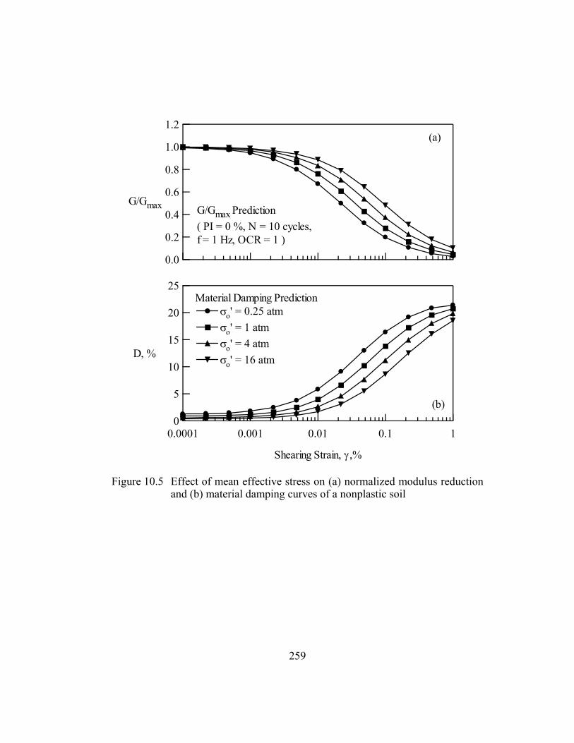
259
1.2
1.0
0.8
0.6
0.4
0.2
0.0
G/Gmax G/Gmax Prediction( PI = 0 %, N = 10 cycles, f = 1 Hz, OCR = 1 )
(a)
25
20
15
10
5
0
D, %
0.0001 0.001 0.01 0.1 1
Shearing Strain, γ ,%
Material Damping Predictionσo' = 0.25 atmσo' = 1 atmσo' = 4 atmσo' = 16 atm
(b)
Figure 10.5 Effect of mean effective stress on (a) normalized modulus reduction and (b) material damping curves of a nonplastic soil
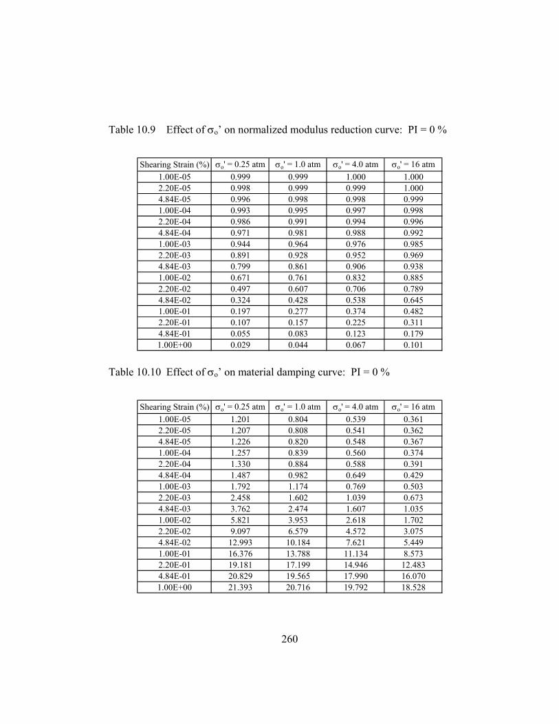
260
Table 10.9 Effect of σo’ on normalized modulus reduction curve: PI = 0 %
Shearing Strain (%) σo' = 0.25 atm σo' = 1.0 atm σo' = 4.0 atm σo' = 16 atm1.00E-05 0.999 0.999 1.000 1.0002.20E-05 0.998 0.999 0.999 1.0004.84E-05 0.996 0.998 0.998 0.9991.00E-04 0.993 0.995 0.997 0.9982.20E-04 0.986 0.991 0.994 0.9964.84E-04 0.971 0.981 0.988 0.9921.00E-03 0.944 0.964 0.976 0.9852.20E-03 0.891 0.928 0.952 0.9694.84E-03 0.799 0.861 0.906 0.9381.00E-02 0.671 0.761 0.832 0.8852.20E-02 0.497 0.607 0.706 0.7894.84E-02 0.324 0.428 0.538 0.6451.00E-01 0.197 0.277 0.374 0.4822.20E-01 0.107 0.157 0.225 0.3114.84E-01 0.055 0.083 0.123 0.1791.00E+00 0.029 0.044 0.067 0.101
Table 10.10 Effect of σo’ on material damping curve: PI = 0 %
Shearing Strain (%) σo' = 0.25 atm σo' = 1.0 atm σo' = 4.0 atm σo' = 16 atm1.00E-05 1.201 0.804 0.539 0.3612.20E-05 1.207 0.808 0.541 0.3624.84E-05 1.226 0.820 0.548 0.3671.00E-04 1.257 0.839 0.560 0.3742.20E-04 1.330 0.884 0.588 0.3914.84E-04 1.487 0.982 0.649 0.4291.00E-03 1.792 1.174 0.769 0.5032.20E-03 2.458 1.602 1.039 0.6734.84E-03 3.762 2.474 1.607 1.0351.00E-02 5.821 3.953 2.618 1.7022.20E-02 9.097 6.579 4.572 3.0754.84E-02 12.993 10.184 7.621 5.4491.00E-01 16.376 13.788 11.134 8.5732.20E-01 19.181 17.199 14.946 12.4834.84E-01 20.829 19.565 17.990 16.0701.00E+00 21.393 20.716 19.792 18.528
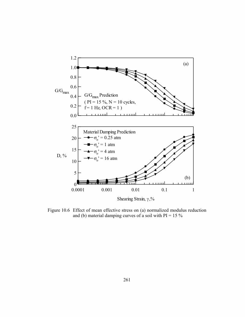
261
1.2
1.0
0.8
0.6
0.4
0.2
0.0
G/Gmax G/Gmax Prediction( PI = 15 %, N = 10 cycles, f = 1 Hz, OCR = 1 )
(a)
25
20
15
10
5
0
D, %
0.0001 0.001 0.01 0.1 1
Shearing Strain, γ ,%
Material Damping Predictionσo' = 0.25 atmσo' = 1 atmσo' = 4 atmσo' = 16 atm
(b)
Figure 10.6 Effect of mean effective stress on (a) normalized modulus reduction and (b) material damping curves of a soil with PI = 15 %

262
Table 10.11 Effect of σo’ on normalized modulus reduction curve: PI = 15 %
Shearing Strain (%) σo' = 0.25 atm σo' = 1.0 atm σo' = 4.0 atm σo' = 16 atm1.00E-05 0.999 1.000 1.000 1.0002.20E-05 0.999 0.999 1.000 1.0004.84E-05 0.997 0.998 0.999 0.9991.00E-04 0.995 0.997 0.998 0.9992.20E-04 0.990 0.993 0.996 0.9974.84E-04 0.979 0.986 0.991 0.9941.00E-03 0.959 0.973 0.983 0.9892.20E-03 0.919 0.947 0.965 0.9774.84E-03 0.847 0.896 0.931 0.9541.00E-02 0.739 0.816 0.873 0.9152.20E-02 0.579 0.682 0.770 0.8394.84E-02 0.400 0.509 0.618 0.7161.00E-01 0.255 0.348 0.454 0.5642.20E-01 0.142 0.205 0.287 0.3864.84E-01 0.074 0.111 0.163 0.2331.00E+00 0.040 0.060 0.091 0.135
Table 10.12 Effect of σo’ on material damping curve: PI = 15 %
Shearing Strain (%) σo' = 0.25 atm σo' = 1.0 atm σo' = 4.0 atm σo' = 16 atm1.00E-05 1.489 0.997 0.668 0.4482.20E-05 1.493 1.000 0.670 0.4494.84E-05 1.506 1.008 0.675 0.4521.00E-04 1.528 1.021 0.683 0.4572.20E-04 1.579 1.053 0.703 0.4694.84E-04 1.690 1.122 0.745 0.4951.00E-03 1.906 1.257 0.829 0.5472.20E-03 2.387 1.562 1.021 0.6674.84E-03 3.358 2.198 1.428 0.9241.00E-02 4.977 3.317 2.173 1.4072.20E-02 7.778 5.440 3.684 2.4334.84E-02 11.489 8.650 6.235 4.3181.00E-01 15.064 12.217 9.482 7.0212.20E-01 18.334 15.951 13.400 10.7804.84E-01 20.515 18.829 16.866 14.6191.00E+00 21.507 20.460 19.158 17.522

263
1.2
1.0
0.8
0.6
0.4
0.2
0.0
G/GmaxG/Gmax Prediction( PI = 30 %, N = 10 cycles, f = 1 Hz, OCR = 1 )
(a)
25
20
15
10
5
0
D, %
0.0001 0.001 0.01 0.1 1
Shearing Strain, γ ,%
Material Damping Predictionσo' = 0.25 atmσo' = 1 atmσo' = 4 atmσo' = 16 atm
(b)
Figure 10.7 Effect of mean effective stress on (a) normalized modulus reduction and (b) material damping curves of a soil with PI = 30 %

264
Table 10.13 Effect of σo’ on normalized modulus reduction curve: PI = 30 %
Shearing Strain (%) σo' = 0.25 atm σo' = 1.0 atm σo' = 4.0 atm σo' = 16 atm1.00E-05 1.000 1.000 1.000 1.0002.20E-05 0.999 0.999 1.000 1.0004.84E-05 0.998 0.999 0.999 0.9991.00E-04 0.996 0.997 0.998 0.9992.20E-04 0.992 0.995 0.997 0.9984.84E-04 0.983 0.989 0.993 0.9961.00E-03 0.968 0.979 0.986 0.9912.20E-03 0.936 0.958 0.972 0.9824.84E-03 0.876 0.917 0.945 0.9641.00E-02 0.783 0.849 0.898 0.9322.20E-02 0.637 0.732 0.810 0.8694.84E-02 0.459 0.569 0.673 0.7631.00E-01 0.303 0.404 0.514 0.6232.20E-01 0.174 0.248 0.339 0.4444.84E-01 0.093 0.137 0.199 0.2791.00E+00 0.050 0.076 0.113 0.166
Table 10.14 Effect of σo’ on material damping curve: PI = 30 %
Shearing Strain (%) σo' = 0.25 atm σo' = 1.0 atm σo' = 4.0 atm σo' = 16 atm1.00E-05 1.778 1.191 0.798 0.5342.20E-05 1.781 1.193 0.799 0.5354.84E-05 1.791 1.199 0.803 0.5381.00E-04 1.808 1.209 0.809 0.5412.20E-04 1.848 1.234 0.824 0.5514.84E-04 1.933 1.287 0.857 0.5711.00E-03 2.101 1.392 0.922 0.6112.20E-03 2.476 1.628 1.070 0.7044.84E-03 3.249 2.128 1.388 0.9031.00E-02 4.581 3.028 1.977 1.2812.20E-02 7.010 4.803 3.206 2.1004.84E-02 10.477 7.664 5.387 3.6591.00E-01 14.088 11.092 8.357 6.0222.20E-01 17.640 14.966 12.231 9.5574.84E-01 20.208 18.185 15.935 13.4721.00E+00 21.542 20.178 18.571 16.655
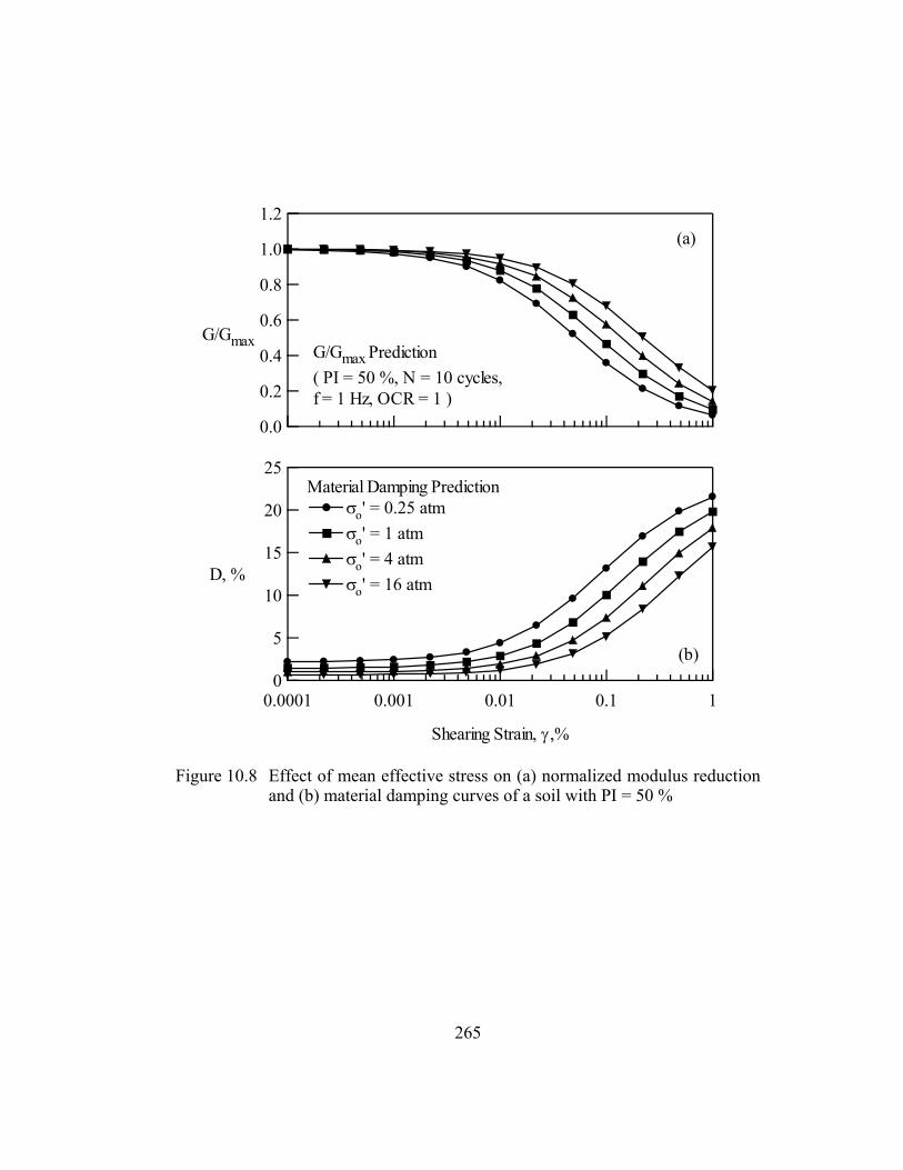
265
1.2
1.0
0.8
0.6
0.4
0.2
0.0
G/GmaxG/Gmax Prediction( PI = 50 %, N = 10 cycles, f = 1 Hz, OCR = 1 )
(a)
25
20
15
10
5
0
D, %
0.0001 0.001 0.01 0.1 1
Shearing Strain, γ ,%
Material Damping Predictionσo' = 0.25 atmσo' = 1 atmσo' = 4 atmσo' = 16 atm
(b)
Figure 10.8 Effect of mean effective stress on (a) normalized modulus reduction and (b) material damping curves of a soil with PI = 50 %
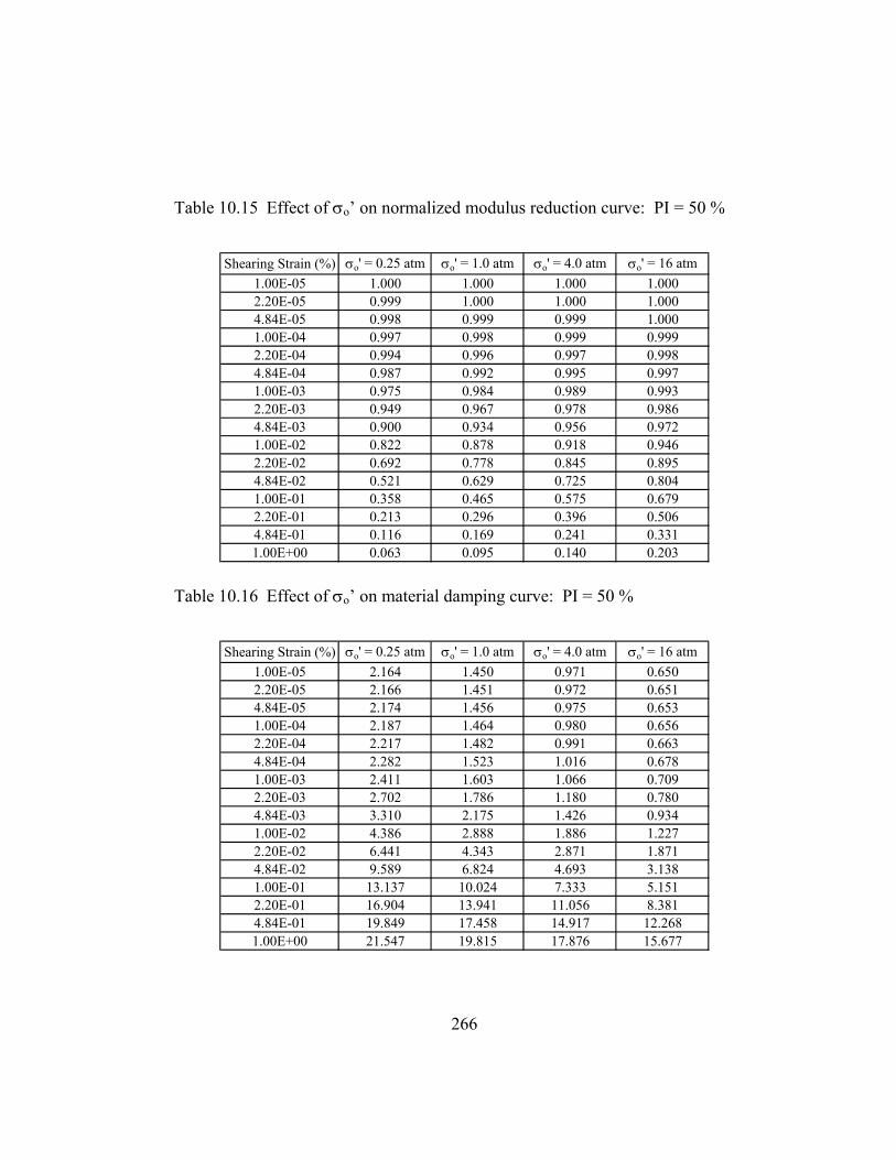
266
Table 10.15 Effect of σo’ on normalized modulus reduction curve: PI = 50 %
Shearing Strain (%) σo' = 0.25 atm σo' = 1.0 atm σo' = 4.0 atm σo' = 16 atm1.00E-05 1.000 1.000 1.000 1.0002.20E-05 0.999 1.000 1.000 1.0004.84E-05 0.998 0.999 0.999 1.0001.00E-04 0.997 0.998 0.999 0.9992.20E-04 0.994 0.996 0.997 0.9984.84E-04 0.987 0.992 0.995 0.9971.00E-03 0.975 0.984 0.989 0.9932.20E-03 0.949 0.967 0.978 0.9864.84E-03 0.900 0.934 0.956 0.9721.00E-02 0.822 0.878 0.918 0.9462.20E-02 0.692 0.778 0.845 0.8954.84E-02 0.521 0.629 0.725 0.8041.00E-01 0.358 0.465 0.575 0.6792.20E-01 0.213 0.296 0.396 0.5064.84E-01 0.116 0.169 0.241 0.3311.00E+00 0.063 0.095 0.140 0.203
Table 10.16 Effect of σo’ on material damping curve: PI = 50 %
Shearing Strain (%) σo' = 0.25 atm σo' = 1.0 atm σo' = 4.0 atm σo' = 16 atm1.00E-05 2.164 1.450 0.971 0.6502.20E-05 2.166 1.451 0.972 0.6514.84E-05 2.174 1.456 0.975 0.6531.00E-04 2.187 1.464 0.980 0.6562.20E-04 2.217 1.482 0.991 0.6634.84E-04 2.282 1.523 1.016 0.6781.00E-03 2.411 1.603 1.066 0.7092.20E-03 2.702 1.786 1.180 0.7804.84E-03 3.310 2.175 1.426 0.9341.00E-02 4.386 2.888 1.886 1.2272.20E-02 6.441 4.343 2.871 1.8714.84E-02 9.589 6.824 4.693 3.1381.00E-01 13.137 10.024 7.333 5.1512.20E-01 16.904 13.941 11.056 8.3814.84E-01 19.849 17.458 14.917 12.2681.00E+00 21.547 19.815 17.876 15.677

267
1.2
1.0
0.8
0.6
0.4
0.2
0.0
G/GmaxG/Gmax Prediction( PI = 100 %, N = 10 cycles, f = 1 Hz, OCR = 1 )
(a)
25
20
15
10
5
0
D, %
0.0001 0.001 0.01 0.1 1
Shearing Strain, γ ,%
Material Damping Predictionσo' = 0.25 atmσo' = 1 atmσo' = 4 atmσo' = 16 atm
(b)
Figure 10.9 Effect of mean effective stress on (a) normalized modulus reduction and (b) material damping curves of a soil with PI = 100 %
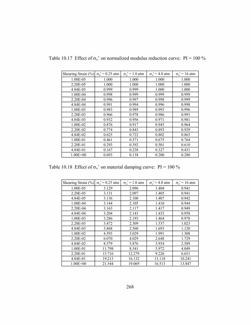
268
Table 10.17 Effect of σo’ on normalized modulus reduction curve: PI = 100 %
Shearing Strain (%) σo' = 0.25 atm σo' = 1.0 atm σo' = 4.0 atm σo' = 16 atm1.00E-05 1.000 1.000 1.000 1.0002.20E-05 1.000 1.000 1.000 1.0004.84E-05 0.999 0.999 1.000 1.0001.00E-04 0.998 0.999 0.999 0.9992.20E-04 0.996 0.997 0.998 0.9994.84E-04 0.991 0.994 0.996 0.9981.00E-03 0.983 0.989 0.993 0.9962.20E-03 0.966 0.978 0.986 0.9914.84E-03 0.932 0.956 0.971 0.9811.00E-02 0.876 0.917 0.945 0.9642.20E-02 0.774 0.843 0.893 0.9294.84E-02 0.625 0.722 0.802 0.8631.00E-01 0.461 0.571 0.675 0.7642.20E-01 0.293 0.392 0.501 0.6104.84E-01 0.167 0.238 0.327 0.4311.00E+00 0.093 0.138 0.200 0.280
Table 10.18 Effect of σo’ on material damping curve: PI = 100 %
Shearing Strain (%) σo' = 0.25 atm σo' = 1.0 atm σo' = 4.0 atm σo' = 16 atm1.00E-05 3.129 2.096 1.404 0.9412.20E-05 3.131 2.097 1.405 0.9414.84E-05 3.136 2.100 1.407 0.9421.00E-04 3.144 2.105 1.410 0.9442.20E-04 3.163 2.117 1.417 0.9494.84E-04 3.204 2.143 1.433 0.9581.00E-03 3.286 2.193 1.464 0.9782.20E-03 3.472 2.309 1.537 1.0234.84E-03 3.868 2.560 1.693 1.1201.00E-02 4.593 3.029 1.991 1.3082.20E-02 6.070 4.029 2.648 1.7294.84E-02 8.579 5.876 3.934 2.5891.00E-01 11.798 8.541 5.972 4.0492.20E-01 15.716 12.279 9.226 6.6514.84E-01 19.213 16.132 13.118 10.2411.00E+00 21.544 19.069 16.513 13.847
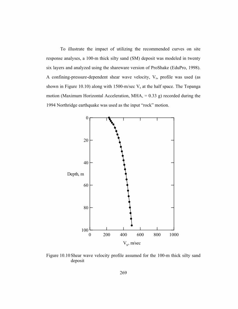
269
To illustrate the impact of utilizing the recommended curves on site
response analyses, a 100-m thick silty sand (SM) deposit was modeled in twenty
six layers and analyzed using the shareware version of ProShake (EduPro, 1998).
A confining-pressure-dependent shear wave velocity, Vs, profile was used (as
shown in Figure 10.10) along with 1500-m/sec Vs at the half space. The Topanga
motion (Maximum Horizontal Acceleration, MHA, = 0.33 g) recorded during the
1994 Northridge earthquake was used as the input “rock” motion.
100
80
60
40
20
0
Depth, m
10008006004002000
Vs, m/sec
Figure 10.10 Shear wave velocity profile assumed for the 100-m thick silty sand deposit
270
In Figure 10.11, the acceleration response spectra from two analyses are
presented: 1) using the average generic curves (Seed et al., 1986) to model all
layers, and 2) using the recommended nonlinear curves interpolated for each soil
layer. The response spectrum of the input motion is also shown in this figure. The
response spectra indicate that the recommended nonlinear curves produce an
MHA much higher than that predicted by the average generic curves (0.54 g vs.
0.37 g). Additionally, larger spectral accelerations (typically 30 % to 50 % higher)
are calculated at all periods less than 1 sec for the analysis utilizing the
recommended nonlinear curves.
As discussed in Darendeli et al. (2001) the impact of utilizing a family of
confining-pressure-dependent curves is expected to be more pronounced for
deeper sites subjected to higher intensity input motions due to lower damping
introduced by the confining-pressure-dependent curves. At longer spectral periods
(T > 1 sec), the response is dominated by the overall stiffness of the site. As a
result, the confining-pressure-dependent analyses may tend to predict a smaller
response at longer periods due to the more linear response modeled by these
curves.
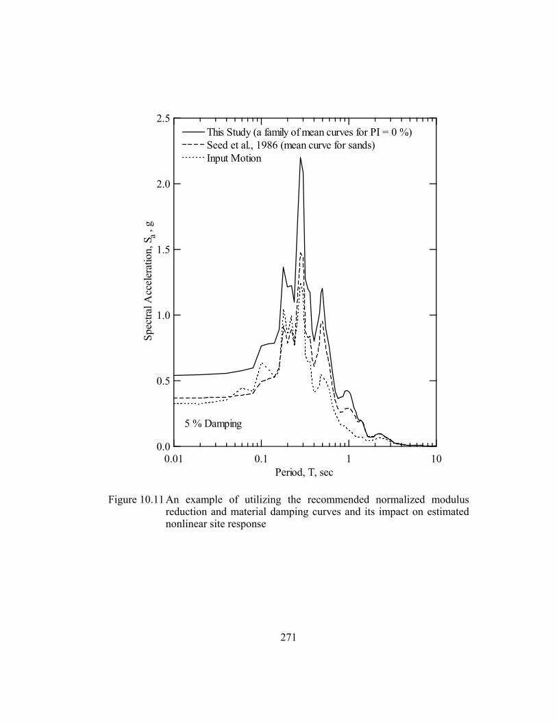
271
2.5
2.0
1.5
1.0
0.5
0.0
Spec
tral A
ccel
erat
ion,
S a ,
g
0.01 0.1 1 10Period, T, sec
This Study (a family of mean curves for PI = 0 %)Seed et al., 1986 (mean curve for sands)Input Motion
5 % Damping
Figure 10.11 An example of utilizing the recommended normalized modulus reduction and material damping curves and its impact on estimated nonlinear site response

272
10.5 SUMMARY
In this chapter, recommended normalized modulus reduction and material
damping curves are presented for soils with a broad range of plasticities confined
over a broad range of mean effective stresses.
The impact of utilizing the recommended curves when assigning nonlinear
soil properties in site response analyses is illustrated by analyzing a 100-m thick
silty sand (SM) deposit using average generic curves (Seed et al., 1986) to model
all twenty six layers, and the recommended nonlinear curves interpolated for each
soil layer. Larger spectral accelerations (typically 30 % to 50 % higher) are
calculated at all periods less than 1 sec for the analysis utilizing the recommended
nonlinear curves than those calculated for the analysis utilizing average generic
curves.

273
CHAPTER 11
UNCERTAINTY ASSOCIATED WITH THE MODEL
PREDICTIONS
11.1 INTRODUCTION
In this chapter, uncertainty associated with the normalized modulus
reduction and material damping curves predicted by the calibrated model is
briefly discussed.
Calculation of standard deviation associated with a point estimate of
normalized shear modulus or material damping ratio, and the covariance structure
of the predicted curves are presented.
Utilization of the calibrated model in probabilistic seismic hazard
assessment is also discussed herein. Integration of random shear-wave velocity
profiles and normalized modulus reduction and material damping curves into
ground motion analysis is recommended. An example regarding incorporation of
the modeled uncertainty (in nonlinear soil behavior) into site response analysis is
also presented.
11.2 UNCERTAINTY IN NONLINEAR SOIL BEHAVIOR
As presented in Chapter Nine, the calibrated model can be utilized to
construct normalized modulus reduction and material damping curves for various
soil types and loading conditions by using the updated mean values of model
parameters (φ1 through φ12) presented in Table 8.12. However, these predicted

274
curves represent average nonlinear curves and the actual data fall into a band of
scatter around these estimates.
At this point, it is important to note that there are two sources of
uncertainty associated with the predicted curves. First, there is uncertainty in the
values of the model parameters. As shown in Table 8.12, where a comparison of
the prior and updated variances of the model parameters are presented, this
component reduces significantly upon calibration of the model.
The second source of uncertainty is the modeled variability (discussed in
Section 7.4.2) of the physical phenomenon. In order to analyze this component of
uncertainty, some of the model parameters (φ13 through φ18) were utilized in
defining the standard deviation and covariance structure of the data (Section
7.4.2) and were simultaneously calibrated utilizing the First-Order, Second-
Moment Bayesian Method.
Table 11.1 presents the predicted mean values and standard deviations
while Table 11.2 presents the covariance structure for a nonplastic soil confined at
1 atm mean effective stress and loaded with ten cycles at 1 Hz accounting for both
components of uncertainty. Tables 11.3 and 11.4 show the same information
predicted by only accounting for modeled variability.

275
Table 11.1 Predicted mean values and standard deviations accounting for uncertainty in the values of model parameters and variability due to modeled uncertainty
Mean Standard Deviation Mean Standard Deviation1 1.00E-05 0.99945 0.01836 0.80434 0.707662 2.20E-05 0.99896 0.01979 0.80816 0.709303 4.84E-05 0.99759 0.02254 0.81958 0.714224 1.00E-04 0.99546 0.02553 0.83859 0.722325 2.20E-04 0.99067 0.03026 0.88404 0.741326 4.84E-04 0.98108 0.03683 0.98172 0.780587 1.00E-03 0.96353 0.04523 1.17383 0.852508 2.20E-03 0.92753 0.05699 1.60166 0.994029 4.84E-03 0.86113 0.07116 2.47409 1.23299
10 1.00E-02 0.76094 0.08438 3.95297 1.5560611 2.20E-02 0.60663 0.09454 6.57873 2.0048512 4.84E-02 0.42765 0.09556 10.18430 2.4924213 1.00E-01 0.27720 0.08784 13.78800 2.8987514 2.20E-01 0.15670 0.07407 17.19890 3.2365815 4.84E-01 0.08259 0.05961 19.56450 3.4514716 1.00E+00 0.04417 0.04818 20.71610 3.55137
Point Number
Normalized Shear Modulus Material Damping Ratio, %Shearing Strain, %

276
Table 11.2 Predicted covariance structure accounting for uncertainty in the values of model parameters and variability due to modeled uncertainty
Point Number 1 2 3 4 5 6 7 8 9 10 11 12 13 14 15 16
1 1.00 0.95 0.90 0.86 0.82 0.78 0.75 0.71 0.68 0.65 0.62 0.59 0.56 0.54 0.51 0.492 0.95 1.00 0.95 0.91 0.86 0.82 0.79 0.75 0.71 0.68 0.65 0.62 0.59 0.56 0.54 0.513 0.90 0.95 1.00 0.95 0.91 0.86 0.83 0.79 0.75 0.72 0.68 0.65 0.62 0.59 0.56 0.544 0.86 0.91 0.95 1.00 0.95 0.90 0.86 0.82 0.78 0.75 0.71 0.68 0.65 0.62 0.59 0.565 0.82 0.86 0.91 0.95 1.00 0.95 0.91 0.86 0.82 0.79 0.75 0.71 0.68 0.65 0.62 0.596 0.78 0.82 0.86 0.90 0.95 1.00 0.95 0.91 0.86 0.83 0.79 0.75 0.72 0.68 0.65 0.627 0.75 0.79 0.83 0.86 0.91 0.95 1.00 0.95 0.90 0.86 0.82 0.78 0.75 0.71 0.68 0.658 0.71 0.75 0.79 0.82 0.86 0.91 0.95 1.00 0.95 0.91 0.86 0.82 0.79 0.75 0.71 0.689 0.68 0.71 0.75 0.78 0.82 0.86 0.90 0.95 1.00 0.95 0.91 0.86 0.83 0.79 0.75 0.72
10 0.65 0.68 0.72 0.75 0.79 0.83 0.86 0.91 0.95 1.00 0.95 0.90 0.86 0.82 0.78 0.7511 0.62 0.65 0.68 0.71 0.75 0.79 0.82 0.86 0.91 0.95 1.00 0.95 0.91 0.86 0.82 0.7912 0.59 0.62 0.65 0.68 0.71 0.75 0.78 0.82 0.86 0.90 0.95 1.00 0.95 0.91 0.86 0.8313 0.56 0.59 0.62 0.65 0.68 0.72 0.75 0.79 0.83 0.86 0.91 0.95 1.00 0.95 0.90 0.8614 0.54 0.56 0.59 0.62 0.65 0.68 0.71 0.75 0.79 0.82 0.86 0.91 0.95 1.00 0.95 0.9115 0.51 0.54 0.56 0.59 0.62 0.65 0.68 0.71 0.75 0.78 0.82 0.86 0.90 0.95 1.00 0.9516 0.49 0.51 0.54 0.56 0.59 0.62 0.65 0.68 0.72 0.75 0.79 0.83 0.86 0.91 0.95 1.00
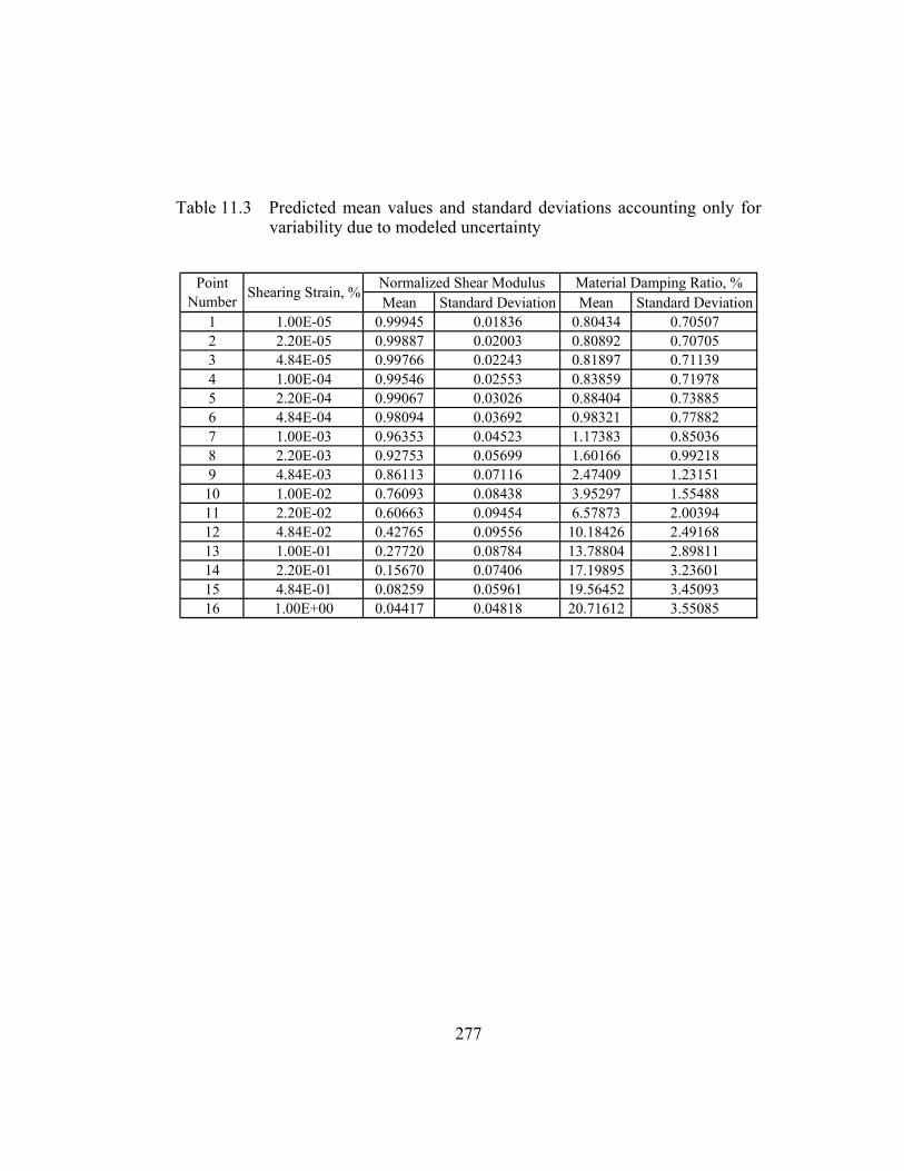
277
Table 11.3 Predicted mean values and standard deviations accounting only for variability due to modeled uncertainty
Mean Standard Deviation Mean Standard Deviation1 1.00E-05 0.99945 0.01836 0.80434 0.705072 2.20E-05 0.99887 0.02003 0.80892 0.707053 4.84E-05 0.99766 0.02243 0.81897 0.711394 1.00E-04 0.99546 0.02553 0.83859 0.719785 2.20E-04 0.99067 0.03026 0.88404 0.738856 4.84E-04 0.98094 0.03692 0.98321 0.778827 1.00E-03 0.96353 0.04523 1.17383 0.850368 2.20E-03 0.92753 0.05699 1.60166 0.992189 4.84E-03 0.86113 0.07116 2.47409 1.2315110 1.00E-02 0.76093 0.08438 3.95297 1.5548811 2.20E-02 0.60663 0.09454 6.57873 2.0039412 4.84E-02 0.42765 0.09556 10.18426 2.4916813 1.00E-01 0.27720 0.08784 13.78804 2.8981114 2.20E-01 0.15670 0.07406 17.19895 3.2360115 4.84E-01 0.08259 0.05961 19.56452 3.4509316 1.00E+00 0.04417 0.04818 20.71612 3.55085
Point Number
Normalized Shear Modulus Material Damping Ratio, %Shearing Strain, %

278
Table 11.4 Predicted covariance structure accounting only for variability due to modeled uncertainty
Point Number 1 2 3 4 5 6 7 8 9 10 11 12 13 14 15 16
1 1.00 0.95 0.90 0.86 0.82 0.78 0.75 0.71 0.68 0.65 0.62 0.59 0.56 0.54 0.51 0.492 0.95 1.00 0.95 0.91 0.86 0.82 0.79 0.75 0.71 0.68 0.65 0.62 0.59 0.56 0.54 0.513 0.90 0.95 1.00 0.95 0.91 0.86 0.83 0.79 0.75 0.72 0.68 0.65 0.62 0.59 0.56 0.544 0.86 0.91 0.95 1.00 0.95 0.90 0.86 0.82 0.78 0.75 0.71 0.68 0.65 0.62 0.59 0.565 0.82 0.86 0.91 0.95 1.00 0.95 0.91 0.86 0.82 0.79 0.75 0.71 0.68 0.65 0.62 0.596 0.78 0.82 0.86 0.90 0.95 1.00 0.95 0.91 0.86 0.83 0.79 0.75 0.72 0.68 0.65 0.627 0.75 0.79 0.83 0.86 0.91 0.95 1.00 0.95 0.90 0.86 0.82 0.78 0.75 0.71 0.68 0.658 0.71 0.75 0.79 0.82 0.86 0.91 0.95 1.00 0.95 0.91 0.86 0.82 0.79 0.75 0.71 0.689 0.68 0.71 0.75 0.78 0.82 0.86 0.90 0.95 1.00 0.95 0.91 0.86 0.83 0.79 0.75 0.72
10 0.65 0.68 0.72 0.75 0.79 0.83 0.86 0.91 0.95 1.00 0.95 0.90 0.86 0.82 0.78 0.7511 0.62 0.65 0.68 0.71 0.75 0.79 0.82 0.86 0.91 0.95 1.00 0.95 0.91 0.86 0.82 0.7912 0.59 0.62 0.65 0.68 0.71 0.75 0.78 0.82 0.86 0.90 0.95 1.00 0.95 0.91 0.86 0.8313 0.56 0.59 0.62 0.65 0.68 0.72 0.75 0.79 0.83 0.86 0.91 0.95 1.00 0.95 0.90 0.8614 0.54 0.56 0.59 0.62 0.65 0.68 0.71 0.75 0.79 0.82 0.86 0.91 0.95 1.00 0.95 0.9115 0.51 0.54 0.56 0.59 0.62 0.65 0.68 0.71 0.75 0.78 0.82 0.86 0.90 0.95 1.00 0.9516 0.49 0.51 0.54 0.56 0.59 0.62 0.65 0.68 0.72 0.75 0.79 0.83 0.86 0.91 0.95 1.00
279
The second set of tables (Tables 11.3 and 11.4) can be obtained by
replacing the model parameters in the equations presented in Section 7.4 with
updated mean values in Table 8.12. However, the first set of tables (Tables 11.1
and 11.2) requires a relatively complicated procedure that incorporates the
updated variance of the model parameters in Table 8.12, updated covariance
structure of the model parameters presented in Table 8.13, and derivatives of
equations utilized in modeling mean values and covariance structure presented in
Section 7.4 with respect to each model parameter. The details of this procedure
are beyond the scope of this study and can be found in Ang and Tang (1990).
The comparison of Tables 11.1 and 11.3 indicates that uncertainty in the
value of model parameters has a negligible impact on point estimates. The errors
introduced by calculating mean values and standard deviations without
accounting for uncertainty in the model parameters are less than about 0.1 % for
the mean values and less than about 1 % for the standard deviations. As a result,
the equations presented in Section 7.4 can be used in calculation of mean values
and standard deviations without introducing significant error due to ignoring
uncertainty regarding the model parameters.
Figure 11.1 shows the predicted mean normalized modulus reduction and
material damping curves and standard deviations of the point estimates tabulated
in Table 11.1. These mean curves are identical to the recommended curves
presented in Chapter Ten for deterministic design applications.

280
1.2
1.0
0.8
0.6
0.4
0.2
0.0
G/Gmax
G/Gmax Predictionσo' = 1 atm, PI = 0 %,N = 10 cycles, f = 1 Hz, OCR = 1
(a)
25
20
15
10
5
0
D, %
0.0001 0.001 0.01 0.1 1
Shearing Strain, γ ,%
Material Damping Predictionσo' = 1 atm, PI = 0 %,N = 10 cycles, f = 1 Hz, OCR = 1
(b)
Figure 11.1 Mean values and standard deviations associated with the point estimates of (a) normalized modulus reduction and (b) material damping curves
281
Besides calculating mean normalized modulus reduction and material
damping curves, the additional information generated by analysis of the data
using the Bayesian approach (rather than an ordinary multivariate nonlinear
optimization procedure) can be utilized in predicting nonlinear curves (random
realizations) consistent with the database for probabilistic site response analysis.
As in the case of mean values and standard deviations, the covariance
structures presented in Tables 11.2 and 11.4 are also quite similar. The errors
introduced by calculating covariance structure without accounting for uncertainty
in the model parameters are less than about 0.1 %. As a result, Equation 7.31
presented in Section 7.4.2 can be used in calculation of correlation coefficients
without introducing significant error due to ignoring uncertainty regarding the
model parameters. At the same time, the covariance structure presented in Table
11.2 is unique to the calibrated model and only changes with the number and
relative amplitudes of shearing strains at which normalized modulus reduction
and material damping curves are generated. In other words, as long as nonlinear
curves are generated at the same sixteen shearing strain amplitudes presented in
Table 11.1, the same covariance structure can be utilized regardless of soil type
and loading conditions.
It is also important to note that the covariance structure in Table 11.2 is
not sensitive to the kind of modeled dynamic soil property. In other words, the
covariance structure does not change significantly whether normalized shear
modulus or material damping ratio is being investigated. The difference between
the covariance structure for the normalized modulus reduction curve and the
282
covariance structure for the material damping curve is less than about 0.1 % and
is a result of added uncertainty regarding the additional parameters utilized in
modeling material damping curve.
At the same time, the model calibration was performed assuming no
correlation between normalized modulus reduction and material damping curves,
although the mean G/Gmax and D curves are coupled to each other. In other words,
the calibrated model relates the material damping curve to the normalized
modulus reduction curve in terms of the average estimates, however, where the
point estimates of material damping ratio are relative to the mean material
damping curve is modeled to be independent from where the point estimates of
normalized shear modulus are relative to the mean normalized modulus reduction
curve.
Briefly, correlated random realizations of normalized modulus reduction
and material damping curves can be separately generated utilizing the covariance
structure calculated based on Equation 7.31 and the mean values of the φ17 and φ18
parameters in Table 8.12. The procedure to generate correlated random
realizations consistent with a given model is beyond the scope of this study and
can be found in Ang and Tang (1990).
A realization of normalized modulus reduction and material damping
curves is presented in Figure 11.2 for the same soil type and loading conditions in
Figure 11.1. The mean curves and one standard deviation ranges of normalized
modulus reduction and material damping curves are shown for comparison
purposes. It is important to note that the scatter of the point estimates is not

283
completely random. Any given point estimate is affected by the location of the
neighboring points relative to the mean curve. This is the result of utilizing a
covariance structure in the random realization process.
1.2
1.0
0.8
0.6
0.4
0.2
0.0
G/GmaxMean Prediction+/- One Standard DeviationRandom Realization
(a)
25
20
15
10
5
0
D, %
0.0001 0.001 0.01 0.1 1
Shearing Strain, γ ,%
Mean Prediction+/- One Standard DeviationRandom Realization
(b)
Figure 11.2 Comparison of the correlated random realization of (a) normalized modulus reduction and (b) material damping curves relative to the mean curves and one standard deviation ranges shown in Figure 11.1
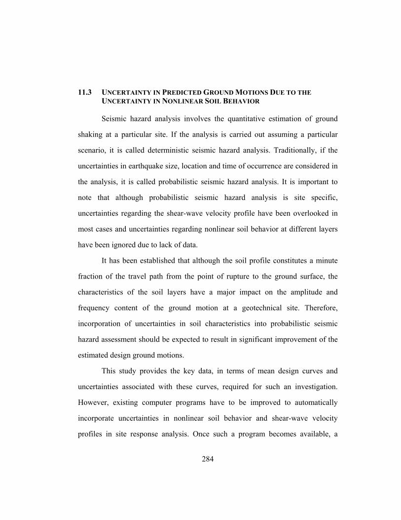
284
11.3 UNCERTAINTY IN PREDICTED GROUND MOTIONS DUE TO THE UNCERTAINTY IN NONLINEAR SOIL BEHAVIOR
Seismic hazard analysis involves the quantitative estimation of ground
shaking at a particular site. If the analysis is carried out assuming a particular
scenario, it is called deterministic seismic hazard analysis. Traditionally, if the
uncertainties in earthquake size, location and time of occurrence are considered in
the analysis, it is called probabilistic seismic hazard analysis. It is important to
note that although probabilistic seismic hazard analysis is site specific,
uncertainties regarding the shear-wave velocity profile have been overlooked in
most cases and uncertainties regarding nonlinear soil behavior at different layers
have been ignored due to lack of data.
It has been established that although the soil profile constitutes a minute
fraction of the travel path from the point of rupture to the ground surface, the
characteristics of the soil layers have a major impact on the amplitude and
frequency content of the ground motion at a geotechnical site. Therefore,
incorporation of uncertainties in soil characteristics into probabilistic seismic
hazard assessment should be expected to result in significant improvement of the
estimated design ground motions.
This study provides the key data, in terms of mean design curves and
uncertainties associated with these curves, required for such an investigation.
However, existing computer programs have to be improved to automatically
incorporate uncertainties in nonlinear soil behavior and shear-wave velocity
profiles in site response analysis. Once such a program becomes available, a
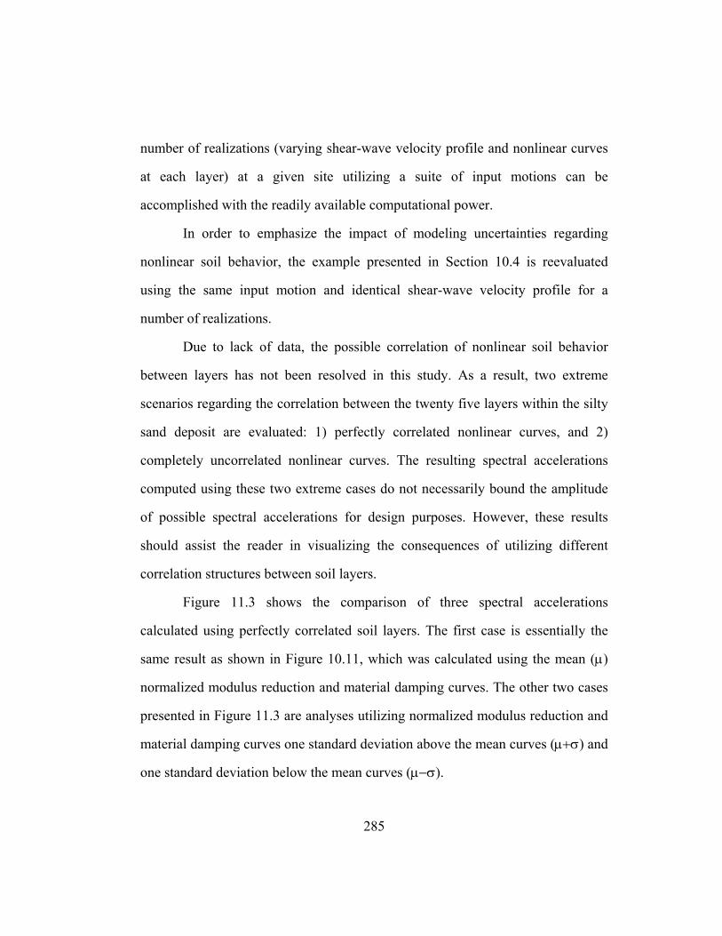
285
number of realizations (varying shear-wave velocity profile and nonlinear curves
at each layer) at a given site utilizing a suite of input motions can be
accomplished with the readily available computational power.
In order to emphasize the impact of modeling uncertainties regarding
nonlinear soil behavior, the example presented in Section 10.4 is reevaluated
using the same input motion and identical shear-wave velocity profile for a
number of realizations.
Due to lack of data, the possible correlation of nonlinear soil behavior
between layers has not been resolved in this study. As a result, two extreme
scenarios regarding the correlation between the twenty five layers within the silty
sand deposit are evaluated: 1) perfectly correlated nonlinear curves, and 2)
completely uncorrelated nonlinear curves. The resulting spectral accelerations
computed using these two extreme cases do not necessarily bound the amplitude
of possible spectral accelerations for design purposes. However, these results
should assist the reader in visualizing the consequences of utilizing different
correlation structures between soil layers.
Figure 11.3 shows the comparison of three spectral accelerations
calculated using perfectly correlated soil layers. The first case is essentially the
same result as shown in Figure 10.11, which was calculated using the mean (µ)
normalized modulus reduction and material damping curves. The other two cases
presented in Figure 11.3 are analyses utilizing normalized modulus reduction and
material damping curves one standard deviation above the mean curves (µ+σ) and
one standard deviation below the mean curves (µ−σ).

286
3.0
2.5
2.0
1.5
1.0
0.5
0.0
Spec
tral A
ccel
erat
ion,
S a ,
g
0.01 0.1 1 10Period, T, sec
Utilizing Mean CurvesUtilizing 1 Standard Deviation Above Average CurvesUtilizing 1 Standard Deviation Below Average Curves
5 % Damping
Figure 11.3 Comparison of spectral accelerations calculated using perfectly correlated soil layers with µ, µ+σ and µ−σ normalized modulus reduction and material damping curves

287
Increasing (or decreasing) the stiffness of all layers in the profile (as a
result of simultaneously shifting normalized modulus reduction curves) should be
expected to have a major impact on site period. In the µ+σ case, an increase in
damping accompanied with an increase in stiffness results in a decrease in
estimated ground motion. In the µ−σ case, the modeled normalized modulus
reduction curves are relatively nonlinear and higher strains are generated at deep
layers. Since material damping increases with strain amplitude, more energy is
dissipated at depth, and estimated ground motion turns out to be generally lower
than that estimated using the mean nonlinear curves.
Figure 11.4 also shows comparison of spectral accelerations calculated
using perfectly correlated soil layers with the result calculated using the mean (µ)
curves shown in Figure 10.11. One of the remaining two spectral accelerations in
this figure is computed utilizing µ+σ normalized modulus reduction curve with
µ−σ material damping curve. The third spectral acceleration is computed
utilizing µ−σ normalized modulus reduction curve with µ+σ material damping
curve. This way, if a layer is modeled to be linear relative to the mean curve in
terms of shear modulus, it is also modeled linear relative to the mean curve in
terms of material damping. In the case of the analysis performed on relatively
linear soil layers, changes in the site period can be identified and the spectral
acceleration is observed to be higher at some lower frequencies. Since the other
case involves relatively nonlinear modulus and damping curves, the resulting
ground motions are lower due to increase in energy dissipation.
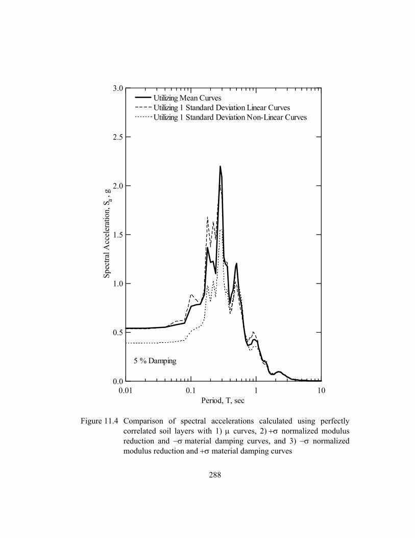
288
3.0
2.5
2.0
1.5
1.0
0.5
0.0
Spec
tral A
ccel
erat
ion,
S a ,
g
0.01 0.1 1 10Period, T, sec
Utilizing Mean CurvesUtilizing 1 Standard Deviation Linear CurvesUtilizing 1 Standard Deviation Non-Linear Curves
5 % Damping
Figure 11.4 Comparison of spectral accelerations calculated using perfectly correlated soil layers with 1) µ curves, 2) +σ normalized modulus reduction and −σ material damping curves, and 3) −σ normalized modulus reduction and +σ material damping curves

289
Fifty realizations utilizing completely uncorrelated nonlinear curves are
presented in Figure 11.5. Although completely uncorrelated soil layers are
unlikely to be a common scenario, the reader must keep in mind the possibility of
missing a thin soft layer during real-life site investigations.
Since the equivalent linear analysis program (EduPro, 1998) utilized in the
analysis is not designed for random realizations, an internal file that contains the
nonlinear curves had to be modified before each run. Although computation time
required for each run was merely about 10 seconds, modification of this file
significantly slowed the process. A number of improvements in site response
analysis programs will be required if they are to be utilized in probabilistic
seismic assessment as recommended.
In Figure 11.5, significantly different spectral accelerations are presented
for a given input motion and shear-wave velocity profile. A single relatively
nonlinear soil layer was observed to reduce surface motions drastically in some of
these realizations. As a result, graphing all spectral accelerations for a large
number of realizations or analyzing histograms of spectral accelerations at certain
periods (Figures 11.6 and 11.7) is recommended rather than analyzing µ, µ+σ,
or µ+2σ spectral accelerations as shown in Figure 11.8. However, a comparison
of the information presented in Figure 11.8 with the result computed utilizing the
mean curves (Figure 11.9) shows that depending on the consequences of failure,
the design acceleration response spectrum may have to be selected much higher
than the deterministic spectrum (estimated utilizing the mean curves) even though
the input motion and the shear-wave velocity profile were fixed in this example.

290
3.0
2.5
2.0
1.5
1.0
0.5
0.0
Spec
tral A
ccel
erat
ion,
S a ,
g
0.01 0.1 1 10Period, T, sec
5 % DampingRandom Realization
Figure 11.5 Fifty realizations of spectral acceleration computed using completely uncorrelated soil layers with randomly generated normalized modulus reduction and material damping curves
291
05
101520253035
0 0.1 0.2 0.3 0.4 0.5 0.6 0.7 0.8 0.9 1Acceleration at 0.1 sec Period, g
Freq
uenc
y(a)
05
101520253035
0 0.25 0.5 0.75 1 1.25 1.5 1.75 2 2.25 2.5Acceleration at 0.3 sec Period, g
Freq
uenc
y
(b)
Figure 11.6 Histograms of spectral accelerations from fifty realizations presented in Figure 11.5 (a) at 0.1 sec and (b) at 0.3 sec
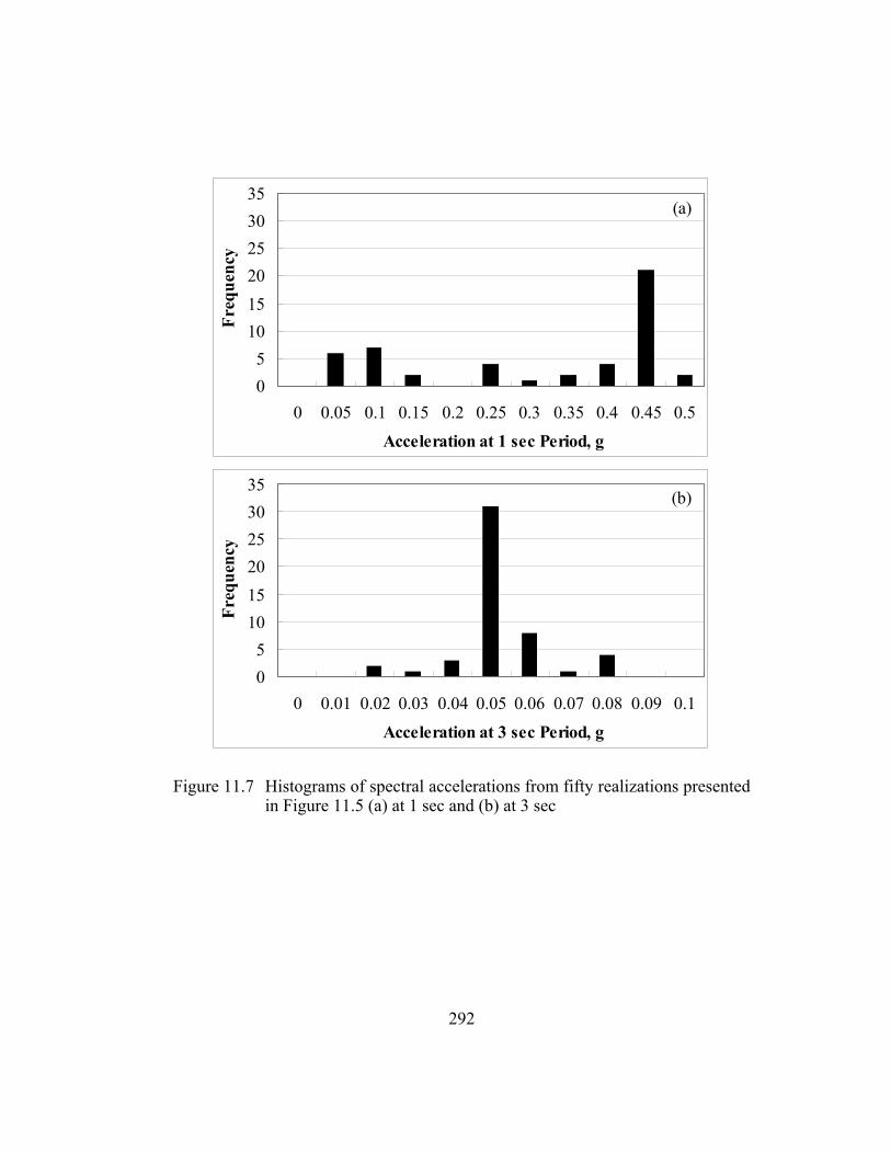
292
05
101520253035
0 0.05 0.1 0.15 0.2 0.25 0.3 0.35 0.4 0.45 0.5Acceleration at 1 sec Period, g
Freq
uenc
y(a)
05
101520253035
0 0.01 0.02 0.03 0.04 0.05 0.06 0.07 0.08 0.09 0.1Acceleration at 3 sec Period, g
Freq
uenc
y
(b)
Figure 11.7 Histograms of spectral accelerations from fifty realizations presented in Figure 11.5 (a) at 1 sec and (b) at 3 sec

293
3.0
2.5
2.0
1.5
1.0
0.5
0.0
Spec
tral A
ccel
erat
ion,
S a ,
g
0.01 0.1 1 10Period, T, sec
Mean of Random RealizationsMean +1 Standard Deviation of Random RealizationsMean +2 Standard Deviation of Random Realizations
5 % Damping
Figure 11.8 Distribution of fifty realizations of spectral acceleration presented in Figure 11.5

294
3.0
2.5
2.0
1.5
1.0
0.5
0.0
Spec
tral A
ccel
erat
ion,
S a ,
g
0.01 0.1 1 10Period, T, sec
Mean of Random RealizationsMean +1 Standard Deviation of Random RealizationsMean +2 Standard Deviation of Random RealizationsUtilizing Mean Curves
5 % Damping
Figure 11.9 Comparison of the spectral accelerations from the fifty realizations with the results computed utilizing mean normalized modulus reduction and material damping curves
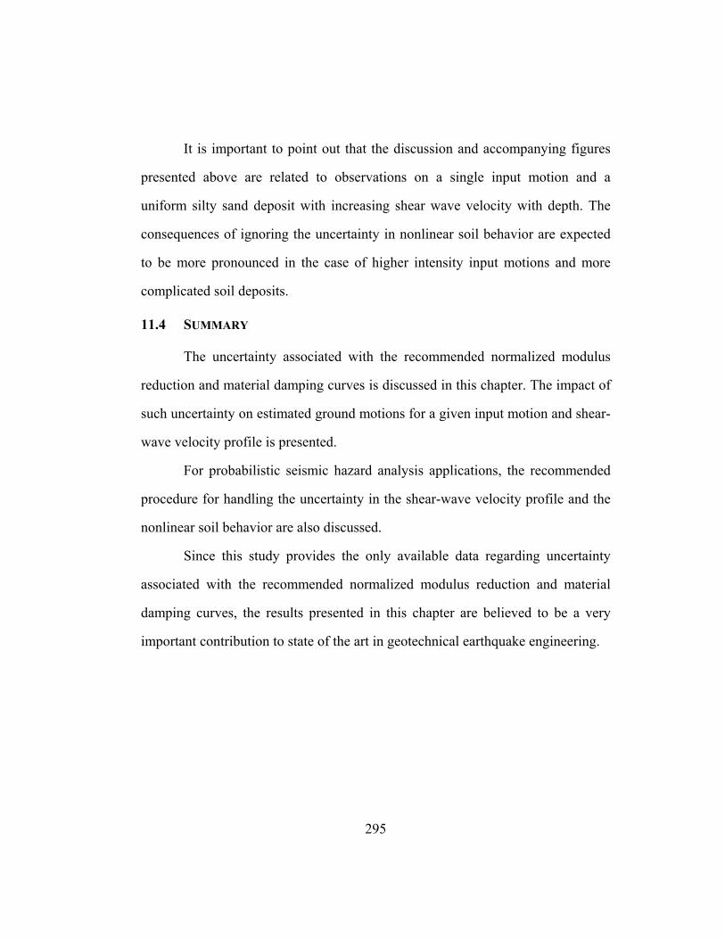
295
It is important to point out that the discussion and accompanying figures
presented above are related to observations on a single input motion and a
uniform silty sand deposit with increasing shear wave velocity with depth. The
consequences of ignoring the uncertainty in nonlinear soil behavior are expected
to be more pronounced in the case of higher intensity input motions and more
complicated soil deposits.
11.4 SUMMARY
The uncertainty associated with the recommended normalized modulus
reduction and material damping curves is discussed in this chapter. The impact of
such uncertainty on estimated ground motions for a given input motion and shear-
wave velocity profile is presented.
For probabilistic seismic hazard analysis applications, the recommended
procedure for handling the uncertainty in the shear-wave velocity profile and the
nonlinear soil behavior are also discussed.
Since this study provides the only available data regarding uncertainty
associated with the recommended normalized modulus reduction and material
damping curves, the results presented in this chapter are believed to be a very
important contribution to state of the art in geotechnical earthquake engineering.

296
CHAPTER 12
SUMMARY AND CONCLUSIONS
12.1 SUMMARY
In this study, the effects of soil type and loading conditions on dynamic
soil properties (presented in terms of normalized shear modulus and material
damping curves) have been quantified based on the data that has been collected at
the University of Texas at Austin over the past decade. Information regarding the
laboratory testing equipment used to collect the data and a general description of
the properties of the specimens included in the database are presented in Chapters
Two and Three, respectively.
The general trends regarding nonlinear soil behavior observed during the
course of this study and reported in the literature are presented in Chapter Four.
Parameters that control nonlinear soil behavior and their relative importance in
terms of affecting normalized modulus reduction and material damping curves
based on general trends observed during the course of this study are presented in
Table 12.1.
Based on the general trends, the successes and shortcomings of various
empirical relationships utilized in the state of practice are evaluated in Chapter
Five and a four-parameter (reference strain, curvature coefficient, small-strain
material damping ratio and the scaling coefficient) soil model that is capable of
capturing these general trends is proposed in Chapter Six (Equation 12.1).

297
Table 12.1 Parameters that control nonlinear soil behavior and their relative importance in terms of affecting normalized modulus reduction and material damping curves based on general trends observed during the course of this study
Parameter Impact on Normalized Modulus Reduction Curve
Impact on Material Damping Curve
Strain Amplitude *** ***Mean Effective Confining Pressure *** ***Soil Type and Plasticity *** ***Number of Loading Cycles *+ ***++
Frequency of Loading (above 1 Hz) * **Overconsolidation Ratio * *Void Ratio * *Degree of Saturation * *Grain Characteristics, Size, Shape, Gradation, Mineralogy * *
*** Very Important + On competent soils included in this study ** Important ++ Soil Type Dependent * Less Important
a
r
GG
+
=
γγ1
1
max
(12.1a)
minsin
1.0
max** DD
GGbD gMaAdjusted +
= (12.1b)
The First-Order, Second-Moment Bayesian Method utilized in the
statistical analysis of the data is discussed in Chapter Seven. An eighteen
parameter model that relates reference strain, curvature coefficient, small-strain
material damping ratio and scaling coefficient to soil type and loading conditions,

298
and that characterizes the covariance structure of the predicted normalized
modulus reduction and material damping curves is also presented in this chapter
(Equation 12.2). 43 '*)**( 21
φφ σφφγ or OCRPI+= (12.2a)
5φ=a (12.2b)
[ ])ln(*1*'*)**( 1076min98 frqOCRPID o φσφφ φφ ++= (12.2c)
)ln(*1211 Nb φφ += (12.2d)
)exp()5.0/(
)exp(25.0)exp(
14
2max
1413 φφ
φσ−
−+=GG
NG (12.2e)
DD *)exp()exp( 1615 φφσ += (12.2f)
))exp(
lnlnexp(*)
)exp(1exp(
1817, φ
γγ
φρ ji
ji
−−−= (12.2g)
Statistical analysis of various subsets of the data and the model calibration
process are briefly described in Chapter Eight.
Chapters Nine and Ten present the equations, graphical solutions, plots
and tables of recommended normalized modulus reduction and material damping
curves for deterministic site-specific analysis. The proposed curves are also
compared with empirical curves widely accepted in state of practice in Chapter
Nine (as shown in Figures 12.1 and 12.2).
Finally, uncertainty associated with the recommended curves is discussed
in Chapter Eleven.

299
1.2
1.0
0.8
0.6
0.4
0.2
0.0
G/Gmax
G/Gmax Prediction( PI = 0 %, N = 10 cycles, f = 1 Hz, OCR = 1 )
(a)
Seed et al. (1986)
25
20
15
10
5
0
D, %
0.0001 0.001 0.01 0.1 1
Shearing Strain, γ ,%
Material Damping Predictionσo' = 0.25 atmσo' = 1 atmσo' = 4 atmσo' = 16 atm
(b)
Figure 12.1 Comparison of the effect of confining pressure on nonlinear soil behavior of sand (PI = 0 %) predicted by the calibrated model and empirical curves proposed for sands by Seed et al. (1986)
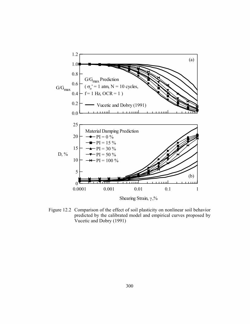
300
1.2
1.0
0.8
0.6
0.4
0.2
0.0
G/Gmax
G/Gmax Prediction( σo' = 1 atm, N = 10 cycles, f = 1 Hz, OCR = 1 )
Vucetic and Dobry (1991)
(a)
25
20
15
10
5
0
D, %
0.0001 0.001 0.01 0.1 1
Shearing Strain, γ ,%
Material Damping PredictionPI = 0 %PI = 15 %PI = 30 %PI = 50 %PI = 100 %
(b)
Figure 12.2 Comparison of the effect of soil plasticity on nonlinear soil behavior predicted by the calibrated model and empirical curves proposed by Vucetic and Dobry (1991)

301
12.2 CONCLUSIONS
A new family of normalized modulus reduction and material damping
design curves is proposed utilizing a four-parameter model calibrated to a rather
large database of resonant column and torsional shear test results. One of the
unique features of this study is the consideration for uncertainty associated with
the recommended curves. Figure 12.3 shows mean values predicted using the
calibrated model and uncertainty associated with these point estimates.
This study is believed to be a valuable contribution to the state of the art
because it provides the means to incorporate the uncertainty in nonlinear soil
behavior into probabilistic seismic hazard analysis. However, utilization of this
work requires improvement of site response analysis programs available at this
point in time.
302
1.2
1.0
0.8
0.6
0.4
0.2
0.0
G/Gmax
G/Gmax Predictionσo' = 1 atm, PI = 0 %,N = 10 cycles, f = 1 Hz, OCR = 1
(a)
25
20
15
10
5
0
D, %
0.0001 0.001 0.01 0.1 1
Shearing Strain, γ ,%
Material Damping Predictionσo' = 1 atm, PI = 0 %,N = 10 cycles, f = 1 Hz, OCR = 1
(b)
Figure 12.3 Mean values and standard deviations associated with the point estimates of (a) normalized modulus reduction and (b) material damping curves

303
APPENDIX A
HEADER FILE
FOR
FIRST ORDER SECOND MOMENT
BAYESIAN ANALYSIS
OF
RESONANT COLUMN
AND
TORSIONAL SHEAR
TEST RESULTS

304
// Modelh.h : Header file for RCTS data // class ModelStructure : public NormLike { public: int nCOV; // Data Indices int nlocation,nsoil,nspecimen,nswv,ndisturbance,npressure,ntest,nPI,nOCR,ne,nconpre,nfrq, nN,nstr,ncorrstr,nTYPE; // Model Indices int iphi1; int iphi2; int iphi3; int iphi4; int iphi5; int iphi6; int iphi7; int iphi8; int iphi9; int iphi10; int iphi11; int iphi12; int istdGa,istdGb,istdDa,istdDb,ithetanugget; int ntheta; iarray itheta; double scalar; void Initialize(DataStructure &Data, int nPhi, int nconst, double *xconst); void Feasible(double *x); void OutputModel(DataStructure &Data, double *x, CString outfilename); void PrintYMean(DataStructure &Data, double *x, CString output); void CalculateYMeanC(DataStructure &Data, double *x, darray &YMeanC, iarray &index); void CalculatedYMeanCiMM(int iv, DataStructure &Data, double *x, darray &dYMeani, iarray &index); void Calculated2YMeanCijMM(int iv, int jv, DataStructure &Data, double *x, darray &dYMeani, darray &dYMeanj, darray &d2YMeanij, iarray &index);

305
void CalculateYCOVC(DataStructure &Data, double *x, darray &YMean, CovMatrix &YCOV, iarray &index); void CalculatedYCOVCiMM(int iv, DataStructure &Data, double *x, darray &YMean, darray &dYMeani, CovMatrix &YCOV, smatrixsolve &dYCOVi, iarray &index); void Calculated2YCOVCijMM(int iv, int jv, DataStructure &Data, double *x, darray &YMean, darray &dYMeani, darray &dYMeanj, darray &d2YMeanij, CovMatrix &YCOV, smatrixsolve &dYCOVi, smatrixsolve &dYCOVj, smatrixsolve &d2YCOVij, iarray &index); double CalculateYrhoab(DataStructure &Data, double *x, int ka, int kb); double YCOVrho(double *tau, double *x); double dYCOVrhoi(int iv, double *tau, double *x); double d2YCOVrhoij(int iv, int jv, double *tau, double *x); };

306
APPENDIX B
MODEL FILE
FOR
FIRST ORDER SECOND MOMENT
BAYESIAN ANALYSIS
OF
RESONANT COLUMN
AND
TORSIONAL SHEAR
TEST RESULTS

307
// Model.cpp : Model for RCTS Data // #include "stdafx.h" #include <afxwin.h> #include <iostream.h> #include <fstream.h> #include <math.h> #include <direct.h> #include <time.h> #include "machh.h" #include "compareh.h" #include "dblash.h" #include "_arrayh.h" #include "_array2h.h" #include "_array3h.h" #include "matrixh.h" #include "smatrixh.h" #include "gmatrixh.h" #include "covmatrixh.h" #include "dblash.h" #include "goldenh.h" #include "rqph.h" #include "Datah.h" #include "NormalLikeh.h" #include "Modelh.h" void ModelStructure::Initialize(DataStructure &Data, int nPhi, int nconst, double *xconst) { /* Data Structure: Data.d[0] = location # (1=Northern CA, 2=Southern CA, 3=South Carolina, 4=Lotung, Taiwan) Data.d[1] = soil type ( 1=sands with fines < 12%, 2=sands with fines > 12% [< 50%], 3=silts, 4=clays) Data.d[2] = specimen # (3 or 4 digit specimen ID UTA-1-C=103, UT-24-F=2406)

308
Data.d[3] = in-situ shear wave velocity (not utilized in this study, a value of 500 is assigned to all specimens) Data.d[4] = shear wave velocity ratio (not utilized in this study, a value of 1.0 is assigned to all specimens) Data.d[5] = pressure # (some specimens are tested at multiple confining pressures) Data.d[6] = test type ( 1.05-1.2=LA_TS, 2=HA_TS1, 3=HA_TS10, 4=HA_RC) Data.d[7] = plasticity index, PI (%) Data.d[8] = overconsolidation ratio, OCR Data.d[9] = void ratio, e Data.d[10] = isotropic effective confining pressure, conpre (atm) Data.d[11] = loading frequency, frq (Hz) Data.d[12] = number of loading cycles, N Data.d[13] = peak strain for modulus, str (%) Data.d[14] = corrected strain for damping (diffrent only in high amplitude RC), corr_str (%) Data.d[15] = indicator of data type ( 0 for normalized modulus, NG 1 for material damping ratio, D) Data.d[16] = experimental observation ( normalized modulus, NG or material damping ratio, D, %)*/ nlocation = 0; /* index in Data.d of sample location */ nsoil = nlocation + 1; /* index in Data.d of soil type */ nspecimen = nsoil + 1; /* index in Data.d of specimen # */ nswv = nspecimen + 1; /* index in Data.d of in-situ shear wave velocity */ ndisturbance = nswv + 1; /* index in Data.d of shear wave velocity ratio (disturbance) */

309
npressure = ndisturbance + 1; /* index in Data.d of pressure # */ ntest = npressure + 1; /* index in Data.d of test type */ nPI = ntest + 1; /* index in Data.d of PI */ nOCR = nPI + 1; /* index in Data.d of OCR */ ne = nOCR + 1; /* index in Data.d of e */ nconpre = ne + 1; /* index in Data.d of conpre */ nfrq = nconpre + 1; /* index in Data.d of frq */ nN = nfrq + 1; /* index in Data.d of N */ nstr = nN + 1; /* index in Data.d of str */ ncorrstr = nstr + 1; /* index in Data.d of corr_str */ nTYPE = ncorrstr + 1; /* index in Data.d of Data Type (G versus D) */ //------------------------------------------- censorcheck = 0; /* 0 = all point measurments, 1 = some censored measurements */ ncflag = 99; /* index in Data.d of censor flag (indicates if measurement is censored, if censorcheck = 1) */ nydown = 99; /* index in Data.d of lower bound measurements, if censorcheck = 1 */ ny = nTYPE + 1; /* index in Data.d of point/upper bound measurements */ ny0 = 0; /* index of first useable data point */ //------------------------------------------- nx = nPhi; /* total number of parameters */ nCOV = nx; /* number of separate (not also used for mean) variance parameters */ nmu = nPhi - nCOV; /* number of separate (not also used for variance) mean parameters */ /* Indices in ModelStructure for the model parameters */ iphi1 = 0; iphi2 = iphi1 + 1; iphi3 = iphi2 + 1; iphi4 = iphi3 + 1; iphi5 = iphi4 + 1; iphi6 = iphi5 + 1; iphi7 = iphi6 + 1; iphi8 = iphi7 + 1; iphi9 = iphi8 + 1;

310
iphi10 = iphi9 + 1; iphi11 = iphi10 + 1; iphi12 = iphi11 + 1; istdGa = iphi12 + 1; /* ln */ istdGb = istdGa + 1; /* ln */ istdDa = istdGb + 1; /* ln */ istdDb = istdDa + 1; /* ln */ ithetanugget = istdDb + 1; /* ln */ ntheta = 5; /* ln */ itheta.construct(ntheta); itheta[0] = ithetanugget + 1; itheta[1] = itheta[0] + 1; itheta[2] = itheta[1] + 1; itheta[3] = itheta[2] + 1; itheta[4] = itheta[3] + 1; /* Scale measurements to avoid numerical precision problems in calculations */ scalar = 1.0; if (censorcheck == 1) dscal(Data.nMeas,scalar,Data.d[nydown],1); dscal(Data.nMeas,scalar,Data.d[ny],1); rhozero = 1.0e-2; /* effective zero value for correlation */ } void ModelStructure::Feasible(double *x) {} void ModelStructure::OutputModel(DataStructure &Data, double *x, CString outfilename) { PrintYMean(Data,x,outfilename); }

311
APPENDIX C
FILE USED IN ESTIMATING MEAN VALUES
FOR
FIRST ORDER SECOND MOMENT
BAYESIAN ANALYSIS
OF
RESONANT COLUMN
AND
TORSIONAL SHEAR
TEST RESULTS

312
// RCTSYMean.cpp : Proposed Equations for RCTS data // #include "stdafx.h" #include <afxwin.h> #include <iostream.h> #include <fstream.h> #include <math.h> #include <direct.h> #include "machh.h" #include "compareh.h" #include "dblash.h" #include "_arrayh.h" #include "_array2h.h" #include "_array3h.h" #include "matrixh.h" #include "smatrixh.h" #include "gmatrixh.h" #include "covmatrixh.h" #include "dblash.h" #include "goldenh.h" #include "rqph.h" #include "Datah.h" #include "NormalLikeh.h" #include "Modelh.h" void ModelStructure::PrintYMean(DataStructure &Data, double *x, CString output) { int n,k; int ytype; double yk; n = Data.nMeas; darray YMean(n); iarray index(n); for (k = 0; k < n; k++) index[k] = k; CalculateYMeanC(Data,x,YMean,index); CovMatrix YCOV(n); CalculateYCOVC(Data,x,YMean,YCOV,index); ofstream out(output);

313
out << "Point" << "\t" << "ytype" << "\t" << "yk" << "\t" << "YMean" << "\t" << "YCOV" "\n"; for (k = 0; k < n; k++) { yk = Data.d[ny][k]; ytype = int(Data.d[nTYPE][k]); out << k << "\t" << ytype << "\t" << yk/scalar << "\t" << YMean[k]/scalar << "\t" << YCOV.G.xptr[k] << "\n"; } out.close(); } void ModelStructure::CalculateYMeanC(DataStructure &Data, double *x, darray &YMeanC, iarray &index) { int kindex,nindex,k; double dbl_par_phi[25];// par stand for model parameters double dbl_atr_str, dbl_atr_corr_str, dbl_atr_PI, dbl_atr_OCR, dbl_atr_e, dbl_atr_Fe, dbl_atr_conpre, dbl_atr_frq, dbl_atr_N; // atr stands for attributes double dbl_refstr, dbl_a, dbl_NG, dbl_NG_corrstr, dbl_DMasing, dbl_c1, dbl_c2, dbl_c3, dbl_Dmin, dbl_b, dbl_D; // Dependent intermediate variables int datatype; double dbl_con_pi = 3.1415926535; //Constant PI nindex = index.n; // total number of nearby data points // assign values to model parameters dbl_par_phi[1] = x[iphi1]; dbl_par_phi[2] = x[iphi2]; dbl_par_phi[3] = x[iphi3]; dbl_par_phi[4] = x[iphi4]; dbl_par_phi[5] = x[iphi5]; dbl_par_phi[6] = x[iphi6]; dbl_par_phi[7] = x[iphi7]; dbl_par_phi[8] = x[iphi8]; dbl_par_phi[9] = x[iphi9]; dbl_par_phi[10] = x[iphi10]; dbl_par_phi[11] = x[iphi11];
314
dbl_par_phi[12] = x[iphi12]; // Step through nearby data set and get YMean for each point for (kindex = 0; kindex < nindex; kindex++) { k = index[kindex]; // assign values to attributes dbl_atr_str = Data.d[nstr][k]; dbl_atr_corr_str = Data.d[ncorrstr][k]; dbl_atr_PI = Data.d[nPI][k]; dbl_atr_OCR = Data.d[nOCR][k]; dbl_atr_e = Data.d[ne][k]; dbl_atr_conpre = Data.d[nconpre][k]; dbl_atr_frq = Data.d[nfrq][k]; dbl_atr_N = Data.d[nN][k]; datatype = int(Data.d[nTYPE][k]); // calculation of normalized modulus and damping values // for given atributes and model parameters // although the effect of void ratio is not accounted for in this study // the code is written so that an F(e) term such as the one below // can be included in the future // dbl_atr_Fe=0.3 + 0.7 * pow (dbl_atr_e,2); dbl_atr_Fe=1.0; dbl_refstr=(dbl_par_phi[1]+dbl_par_phi[2]*dbl_atr_PI*pow(dbl_atr_OCR,dbl_par_phi[3])) *dbl_atr_Fe*pow(dbl_atr_conpre,dbl_par_phi[4]); dbl_a=dbl_par_phi[5]; dbl_NG=1.0/(1+pow((dbl_atr_str/dbl_refstr),dbl_a)); dbl_NG_corrstr=1.0/(1+pow((dbl_atr_corr_str/dbl_refstr),dbl_a)); dbl_DMasing=(100.0/dbl_con_pi)*(4*(dbl_atr_corr_str-dbl_refstr*log((dbl_atr_corr_str+dbl_refstr)/dbl_refstr))

315
/(pow(dbl_atr_corr_str,2)/(dbl_atr_corr_str+dbl_refstr))-2); dbl_c1= -1.1143*pow(dbl_a,2)+1.8618*dbl_a+0.2523; dbl_c2= 0.0805*pow(dbl_a,2)-0.0710*dbl_a-0.0095; dbl_c3= -0.0005*pow(dbl_a,2)+0.0002*dbl_a+0.0003; dbl_Dmin= (dbl_par_phi[6]+dbl_par_phi[7]*dbl_atr_PI*pow(dbl_atr_OCR,dbl_par_phi[8])) *pow(dbl_atr_conpre,dbl_par_phi[9])*(1+dbl_par_phi[10]*log(dbl_atr_frq)); dbl_b=dbl_par_phi[11]+dbl_par_phi[12]*log(dbl_atr_N); dbl_D=dbl_Dmin+dbl_b*pow(dbl_NG_corrstr,0.1)*(dbl_c1*dbl_DMasing+dbl_c2*pow(dbl_DMasing,2) +dbl_c3*pow(dbl_DMasing,3)); if (datatype == 0) { YMeanC[kindex] = scalar*dbl_NG; } else { YMeanC[kindex] = scalar*dbl_D; } } // for (kindex = 0; kindex < nindex; kindex++) } void ModelStructure::CalculatedYMeanCiMM(int iv, DataStructure &Data, double *x, darray &dYMeani, iarray &index) { int k,kindex,nindex;

316
double dbl_par_phi[25], dbl_par_dphi[25]; // par stand for model parameters double dbl_atr_str, dbl_atr_corr_str, dbl_atr_PI, dbl_atr_OCR, dbl_atr_e, dbl_atr_Fe, dbl_atr_conpre, dbl_atr_frq, dbl_atr_N; // atr stands for attributes double dbl_refstr, dbl_a, dbl_NG, dbl_NG_corrstr, dbl_DMasing, dbl_c1, dbl_c2, dbl_c3, dbl_Dmin, dbl_b, dbl_D; // Dependent intermediate variables double dbl_drefstr, dbl_da, dbl_dNG, dbl_dNG_corrstr, dbl_dc1, dbl_dc2, dbl_dc3, dbl_dDMasing, dbl_dDmin, dbl_db, dbl_dD; // First Order Partial Derivative of dependent intermediate variables int datatype; int int_loopcounter_i,int_loopcounter_j; double dbl_con_pi = 3.1415926535; //Constant PI nindex = index.n; // assign values to model parameters dbl_par_phi[1] = x[iphi1]; dbl_par_phi[2] = x[iphi2]; dbl_par_phi[3] = x[iphi3]; dbl_par_phi[4] = x[iphi4]; dbl_par_phi[5] = x[iphi5]; dbl_par_phi[6] = x[iphi6]; dbl_par_phi[7] = x[iphi7]; dbl_par_phi[8] = x[iphi8]; dbl_par_phi[9] = x[iphi9]; dbl_par_phi[10] = x[iphi10]; dbl_par_phi[11] = x[iphi11]; dbl_par_phi[12] = x[iphi12]; // set all dphi equal to zero for (int_loopcounter_j=0;int_loopcounter_j<nx;int_loopcounter_j++) { dbl_par_dphi[int_loopcounter_j]=0; } // calculation of first order derivatives for iv int_loopcounter_i=iv+1; // calculate derivatives for phi[int_loopcounter_i]

317
dbl_par_dphi[int_loopcounter_i]=1; for (kindex = 0; kindex < nindex; kindex++) { k = index[kindex]; // assign values to attributes dbl_atr_str= Data.d[nstr][k]; dbl_atr_corr_str= Data.d[ncorrstr][k]; dbl_atr_PI= Data.d[nPI][k]; dbl_atr_OCR= Data.d[nOCR][k]; dbl_atr_e= Data.d[ne][k]; dbl_atr_conpre= Data.d[nconpre][k]; dbl_atr_frq= Data.d[nfrq][k]; dbl_atr_N= Data.d[nN][k]; datatype = int(Data.d[nTYPE][k]); // calculation of normalized modulus and damping values // for given atributes and model parameters // although the effect of void ratio is not accounted for in this study // the code is written so that an F(e) term such as the one below // can be included in the future // dbl_atr_Fe=0.3 + 0.7 * pow (dbl_atr_e,2); dbl_atr_Fe=1.0; dbl_refstr=(dbl_par_phi[1]+dbl_par_phi[2]*dbl_atr_PI*pow(dbl_atr_OCR,dbl_par_phi[3])) *dbl_atr_Fe*pow(dbl_atr_conpre,dbl_par_phi[4]); dbl_a=dbl_par_phi[5]; dbl_NG=1.0/(1+pow((dbl_atr_str/dbl_refstr),dbl_a)); dbl_NG_corrstr=1.0/(1+pow((dbl_atr_corr_str/dbl_refstr),dbl_a)); dbl_DMasing=(100.0/dbl_con_pi)*(4*(dbl_atr_corr_str-dbl_refstr*log((dbl_atr_corr_str+dbl_refstr)/dbl_refstr))

318
/(pow(dbl_atr_corr_str,2)/(dbl_atr_corr_str+dbl_refstr))-2); dbl_c1= -1.1143*pow(dbl_a,2)+1.8618*dbl_a+0.2523; dbl_c2= 0.0805*pow(dbl_a,2)-0.0710*dbl_a-0.0095; dbl_c3= -0.0005*pow(dbl_a,2)+0.0002*dbl_a+0.0003; dbl_Dmin= (dbl_par_phi[6]+dbl_par_phi[7]*dbl_atr_PI*pow(dbl_atr_OCR,dbl_par_phi[8])) *pow(dbl_atr_conpre,dbl_par_phi[9])*(1+dbl_par_phi[10]*log(dbl_atr_frq)); dbl_b=dbl_par_phi[11]+dbl_par_phi[12]*log(dbl_atr_N); dbl_D=dbl_Dmin+dbl_b*pow(dbl_NG_corrstr,0.1)*(dbl_c1*dbl_DMasing+dbl_c2*pow(dbl_DMasing,2) +dbl_c3*pow(dbl_DMasing,3)); //"FIRST ORDER DERIVATIVES" CODE FOR phi[int_loopcounter_i] //------------------------------------------------------- dbl_drefstr=dbl_atr_Fe*pow(dbl_atr_conpre,dbl_par_phi[4])*dbl_par_dphi[1] +dbl_atr_PI*pow(dbl_atr_OCR,dbl_par_phi[3])*dbl_atr_Fe*pow(dbl_atr_conpre,dbl_par_phi[4])*dbl_par_dphi[2] +dbl_par_phi[2]*dbl_atr_PI*pow(dbl_atr_OCR,dbl_par_phi[3])*log(dbl_atr_OCR)*dbl_atr_Fe*pow(dbl_atr_conpre,dbl_par_phi[4])*dbl_par_dphi[3] +(dbl_par_phi[1]+dbl_par_phi[2]*dbl_atr_PI*pow(dbl_atr_OCR,dbl_par_phi[3]))*dbl_atr_Fe*pow(dbl_atr_conpre,dbl_par_phi[4])*log(dbl_atr_conpre)*dbl_par_dphi[4]; dbl_da=dbl_par_dphi[5];
319
dbl_dNG=(1/pow((1+pow((dbl_atr_str/dbl_refstr),dbl_a)),2))*pow((dbl_atr_str/dbl_refstr),dbl_a)*(dbl_a/dbl_refstr)*dbl_drefstr +(-1/pow((1+pow((dbl_atr_str/dbl_refstr),dbl_a)),2))*pow((dbl_atr_str/dbl_refstr),dbl_a)*log(dbl_atr_str/dbl_refstr)*dbl_da; dbl_dNG_corrstr=(1/pow((1+pow((dbl_atr_corr_str/dbl_refstr),dbl_a)),2))*pow((dbl_atr_corr_str/dbl_refstr),dbl_a)*(dbl_a/dbl_refstr)*dbl_drefstr +(-1/pow((1+pow((dbl_atr_corr_str/dbl_refstr),dbl_a)),2))*pow((dbl_atr_corr_str/dbl_refstr),dbl_a)*log(dbl_atr_corr_str/dbl_refstr)*dbl_da; dbl_dc1=(-2.2286*dbl_a+1.8618)*dbl_da; dbl_dc2=( 0.1610*dbl_a-0.0710)*dbl_da; dbl_dc3=(-0.0010*dbl_a+0.0002)*dbl_da; dbl_dDMasing=(-400)*((log((dbl_atr_corr_str+dbl_refstr)/dbl_refstr)*dbl_atr_corr_str +2*dbl_refstr*log((dbl_atr_corr_str+dbl_refstr)/dbl_refstr) -2*dbl_atr_corr_str)/(pow(dbl_atr_corr_str,2)*dbl_con_pi)) *dbl_drefstr; dbl_dDmin=pow(dbl_atr_conpre,dbl_par_phi[9])*(1+dbl_par_phi[10]*log(dbl_atr_frq))*dbl_par_dphi[6] +dbl_atr_PI*pow(dbl_atr_OCR,dbl_par_phi[8])*pow(dbl_atr_conpre,dbl_par_phi[9])*(1+dbl_par_phi[10]*log(dbl_atr_frq))*dbl_par_dphi[7] +dbl_par_phi[7]*dbl_atr_PI*pow(dbl_atr_OCR,dbl_par_phi[8])*log(dbl_atr_OCR)*pow(dbl_atr_conpre,dbl_par_phi[9])*(1+dbl_par_phi[10]*log(dbl_atr_frq))*dbl_par_dphi[8] +(dbl_par_phi[6]+dbl_par_phi[7]*dbl_atr_PI*pow(dbl_atr_OCR,dbl_par_phi[8]))*pow(dbl_atr_conpre,dbl_par_phi[9])*log(dbl_atr_conpre)*(1+dbl_par_phi[10]*log(dbl_atr_frq))*dbl_par_dphi[9]

320
+(dbl_par_phi[6]+dbl_par_phi[7]*dbl_atr_PI*pow(dbl_atr_OCR,dbl_par_phi[8]))*pow(dbl_atr_conpre,dbl_par_phi[9])*log(dbl_atr_frq)*dbl_par_dphi[10]; dbl_db=dbl_par_dphi[11]+log(dbl_atr_N)*dbl_par_dphi[12]; dbl_dD=dbl_dDmin +pow(dbl_NG_corrstr,0.1)*dbl_DMasing*(dbl_c1+dbl_c2*dbl_DMasing+dbl_c3*pow(dbl_DMasing,2))*dbl_db +0.1*dbl_b*dbl_DMasing*((dbl_c1+dbl_c2*dbl_DMasing+dbl_c3*pow(dbl_DMasing,2))/pow(dbl_NG_corrstr,0.9))*dbl_dNG_corrstr +dbl_b*pow(dbl_NG_corrstr,0.1)*(dbl_c1+2*dbl_c2*dbl_DMasing+3*dbl_c3*pow(dbl_DMasing,2))*dbl_dDMasing +dbl_b*pow(dbl_NG_corrstr,0.1)*dbl_DMasing*dbl_dc1 +dbl_b*pow(dbl_NG_corrstr,0.1)*pow(dbl_DMasing,2)*dbl_dc2 +dbl_b*pow(dbl_NG_corrstr,0.1)*pow(dbl_DMasing,3)*dbl_dc3; //------------------------------------------------------- if (datatype == 0) { dYMeani[kindex] = scalar*dbl_dNG; } else { dYMeani[kindex] = scalar*dbl_dD; } } // for (kindex = 0; kindex < nindex; kindex++) } void ModelStructure::Calculated2YMeanCijMM(int iv, int jv, DataStructure &Data, double *x,
321
darray &dYMeani, darray &dYMeanj, darray &d2YMeanij, iarray &index) { int k,kindex,nindex; double dbl_par_phi[25], dbl_par_diphi[25], dbl_par_djphi[25]; // par stand for model parameters double dbl_atr_str, dbl_atr_corr_str, dbl_atr_PI, dbl_atr_OCR, dbl_atr_e, dbl_atr_Fe, dbl_atr_conpre, dbl_atr_frq, dbl_atr_N; // atr stands for attributes double dbl_refstr, dbl_a, dbl_NG, dbl_NG_corrstr, dbl_DMasing, dbl_c1, dbl_c2, dbl_c3, dbl_Dmin, dbl_b, dbl_D; // Dependent intermediate variables double dbl_direfstr, dbl_dia, dbl_diNG, dbl_diNG_corrstr, dbl_dic1, dbl_dic2, dbl_dic3, dbl_diDMasing, dbl_diDmin, dbl_dib, dbl_diD; // diNG stands for first order partial derivative of NG with respect to phi[i] double dbl_djrefstr, dbl_dja, dbl_djNG, dbl_djNG_corrstr, dbl_djc1, dbl_djc2, dbl_djc3, dbl_djDMasing, dbl_djDmin, dbl_djb, dbl_djD; // djNG stands for first order partial derivative of NG with respect to phi[j] double dbl_d2refstr, dbl_d2a, dbl_d2NG, dbl_d2NG_corrstr, dbl_d2c1, dbl_d2c2, dbl_d2c3, dbl_d2DMasing, dbl_d2Dmin, dbl_d2b, dbl_d2D; // d2NG stands for second order partial derivative of NG with respect to phi[i]=phi[j] int datatype; int int_loopcounter_k,int_loopcounter_l,int_loopcounter_m,int_loopcounter_n; double dbl_con_pi = 3.1415926535; //Constant PI nindex = index.n; // assign values to model parameters dbl_par_phi[1] = x[iphi1]; dbl_par_phi[2] = x[iphi2]; dbl_par_phi[3] = x[iphi3]; dbl_par_phi[4] = x[iphi4]; dbl_par_phi[5] = x[iphi5]; dbl_par_phi[6] = x[iphi6]; dbl_par_phi[7] = x[iphi7]; dbl_par_phi[8] = x[iphi8]; dbl_par_phi[9] = x[iphi9]; dbl_par_phi[10] = x[iphi10];
322
dbl_par_phi[11] = x[iphi11]; dbl_par_phi[12] = x[iphi12]; // set all diphi equal to zero for (int_loopcounter_l=0;int_loopcounter_l<nx;int_loopcounter_l++) { dbl_par_diphi[int_loopcounter_l]=0; } // set all djphi equal to zero for (int_loopcounter_n=0;int_loopcounter_n<nx;int_loopcounter_n++) { dbl_par_djphi[int_loopcounter_n]=0; } // calculation of second order derivatives (d/diphi[int_loopcounter_k]*djphi[int_loopcounter_m]) // calculation of second order derivatives for iv, jv int_loopcounter_k=iv+1; int_loopcounter_m=jv+1; // calculate derivatives for iphi[int_loopcounter_k] dbl_par_diphi[int_loopcounter_k]=1; // calculate derivatives for jphi[int_loopcounter_m] dbl_par_djphi[int_loopcounter_m]=1; for (kindex = 0; kindex < nindex; kindex++) { k = index[kindex]; // assign values to attributes dbl_atr_str= Data.d[nstr][k]; dbl_atr_corr_str= Data.d[ncorrstr][k]; dbl_atr_PI= Data.d[nPI][k]; dbl_atr_OCR= Data.d[nOCR][k]; dbl_atr_e= Data.d[ne][k]; dbl_atr_conpre= Data.d[nconpre][k]; dbl_atr_frq= Data.d[nfrq][k]; dbl_atr_N= Data.d[nN][k]; datatype = int(Data.d[nTYPE][k]);

323
// calculation of normalized modulus and damping values // for given atributes and model parameters // although the effect of void ratio is not accounted for in this study // the code is written so that an F(e) term such as the one below // can be included in the future // dbl_atr_Fe=0.3 + 0.7 * pow (dbl_atr_e,2); dbl_atr_Fe=1.0; dbl_refstr=(dbl_par_phi[1]+dbl_par_phi[2]*dbl_atr_PI*pow(dbl_atr_OCR,dbl_par_phi[3])) *dbl_atr_Fe*pow(dbl_atr_conpre,dbl_par_phi[4]); dbl_a=dbl_par_phi[5]; dbl_NG=1.0/(1+pow((dbl_atr_str/dbl_refstr),dbl_a)); dbl_NG_corrstr=1.0/(1+pow((dbl_atr_corr_str/dbl_refstr),dbl_a)); dbl_DMasing=(100.0/dbl_con_pi)*(4*(dbl_atr_corr_str-dbl_refstr*log((dbl_atr_corr_str+dbl_refstr)/dbl_refstr)) /(pow(dbl_atr_corr_str,2)/(dbl_atr_corr_str+dbl_refstr))-2); dbl_c1= -1.1143*pow(dbl_a,2)+1.8618*dbl_a+0.2523; dbl_c2= 0.0805*pow(dbl_a,2)-0.0710*dbl_a-0.0095; dbl_c3= -0.0005*pow(dbl_a,2)+0.0002*dbl_a+0.0003; dbl_Dmin= (dbl_par_phi[6]+dbl_par_phi[7]*dbl_atr_PI*pow(dbl_atr_OCR,dbl_par_phi[8])) *pow(dbl_atr_conpre,dbl_par_phi[9])*(1+dbl_par_phi[10]*log(dbl_atr_frq)); dbl_b=dbl_par_phi[11]+dbl_par_phi[12]*log(dbl_atr_N);
324
dbl_D=dbl_Dmin+dbl_b*pow(dbl_NG_corrstr,0.1)*(dbl_c1*dbl_DMasing+dbl_c2*pow(dbl_DMasing,2) +dbl_c3*pow(dbl_DMasing,3)); //"FIRST ORDER DERIVATIVES" CODE FOR iphi[int_loopcounter_k] //------------------------------------------------------- dbl_direfstr=dbl_atr_Fe*pow(dbl_atr_conpre,dbl_par_phi[4])*dbl_par_diphi[1] +dbl_atr_PI*pow(dbl_atr_OCR,dbl_par_phi[3])*dbl_atr_Fe*pow(dbl_atr_conpre,dbl_par_phi[4])*dbl_par_diphi[2] +dbl_par_phi[2]*dbl_atr_PI*pow(dbl_atr_OCR,dbl_par_phi[3])*log(dbl_atr_OCR)*dbl_atr_Fe*pow(dbl_atr_conpre,dbl_par_phi[4])*dbl_par_diphi[3] +(dbl_par_phi[1]+dbl_par_phi[2]*dbl_atr_PI*pow(dbl_atr_OCR,dbl_par_phi[3]))*dbl_atr_Fe*pow(dbl_atr_conpre,dbl_par_phi[4])*log(dbl_atr_conpre)*dbl_par_diphi[4]; dbl_dia=dbl_par_diphi[5]; dbl_diNG=(1/pow((1+pow((dbl_atr_str/dbl_refstr),dbl_a)),2))*pow((dbl_atr_str/dbl_refstr),dbl_a)*(dbl_a/dbl_refstr)*dbl_direfstr +(-1/pow((1+pow((dbl_atr_str/dbl_refstr),dbl_a)),2))*pow((dbl_atr_str/dbl_refstr),dbl_a)*log(dbl_atr_str/dbl_refstr)*dbl_dia; dbl_diNG_corrstr=(1/pow((1+pow((dbl_atr_corr_str/dbl_refstr),dbl_a)),2))*pow((dbl_atr_corr_str/dbl_refstr),dbl_a)*(dbl_a/dbl_refstr)*dbl_direfstr +(-1/pow((1+pow((dbl_atr_corr_str/dbl_refstr),dbl_a)),2))*pow((dbl_atr_corr_str/dbl_refstr),dbl_a)*log(dbl_atr_corr_str/dbl_refstr)*dbl_dia; dbl_dic1=(-2.2286*dbl_a+1.8618)*dbl_dia; dbl_dic2=( 0.1610*dbl_a-0.0710)*dbl_dia; dbl_dic3=(-0.0010*dbl_a+0.0002)*dbl_dia;

325
dbl_diDMasing=(-400)*((log((dbl_atr_corr_str+dbl_refstr)/dbl_refstr)*dbl_atr_corr_str +2*dbl_refstr*log((dbl_atr_corr_str+dbl_refstr)/dbl_refstr) -2*dbl_atr_corr_str)/(pow(dbl_atr_corr_str,2)*dbl_con_pi)) *dbl_direfstr; dbl_diDmin=pow(dbl_atr_conpre,dbl_par_phi[9])*(1+dbl_par_phi[10]*log(dbl_atr_frq))*dbl_par_diphi[6] +dbl_atr_PI*pow(dbl_atr_OCR,dbl_par_phi[8])*pow(dbl_atr_conpre,dbl_par_phi[9])*(1+dbl_par_phi[10]*log(dbl_atr_frq))*dbl_par_diphi[7] +dbl_par_phi[7]*dbl_atr_PI*pow(dbl_atr_OCR,dbl_par_phi[8])*log(dbl_atr_OCR)*pow(dbl_atr_conpre,dbl_par_phi[9])*(1+dbl_par_phi[10]*log(dbl_atr_frq))*dbl_par_diphi[8] +(dbl_par_phi[6]+dbl_par_phi[7]*dbl_atr_PI*pow(dbl_atr_OCR,dbl_par_phi[8]))*pow(dbl_atr_conpre,dbl_par_phi[9])*log(dbl_atr_conpre)*(1+dbl_par_phi[10]*log(dbl_atr_frq))*dbl_par_diphi[9] +(dbl_par_phi[6]+dbl_par_phi[7]*dbl_atr_PI*pow(dbl_atr_OCR,dbl_par_phi[8]))*pow(dbl_atr_conpre,dbl_par_phi[9])*log(dbl_atr_frq)*dbl_par_diphi[10]; dbl_dib=dbl_par_diphi[11]+log(dbl_atr_N)*dbl_par_diphi[12]; dbl_diD=dbl_diDmin +pow(dbl_NG_corrstr,0.1)*dbl_DMasing*(dbl_c1+dbl_c2*dbl_DMasing+dbl_c3*pow(dbl_DMasing,2))*dbl_dib +0.1*dbl_b*dbl_DMasing*((dbl_c1+dbl_c2*dbl_DMasing+dbl_c3*pow(dbl_DMasing,2))/pow(dbl_NG_corrstr,0.9))*dbl_diNG_corrstr +dbl_b*pow(dbl_NG_corrstr,0.1)*(dbl_c1+2*dbl_c2*dbl_DMasing+3*dbl_c3*pow(dbl_DMasing,2))*dbl_diDMasing +dbl_b*pow(dbl_NG_corrstr,0.1)*dbl_DMasing*dbl_dic1
326
+dbl_b*pow(dbl_NG_corrstr,0.1)*pow(dbl_DMasing,2)*dbl_dic2 +dbl_b*pow(dbl_NG_corrstr,0.1)*pow(dbl_DMasing,3)*dbl_dic3; //------------------------------------------------------- //"FIRST ORDER DERIVATIVES" CODE FOR jphi[int_loopcounter_m] //------------------------------------------------------- dbl_djrefstr=dbl_atr_Fe*pow(dbl_atr_conpre,dbl_par_phi[4])*dbl_par_djphi[1] +dbl_atr_PI*pow(dbl_atr_OCR,dbl_par_phi[3])*dbl_atr_Fe*pow(dbl_atr_conpre,dbl_par_phi[4])*dbl_par_djphi[2] +dbl_par_phi[2]*dbl_atr_PI*pow(dbl_atr_OCR,dbl_par_phi[3])*log(dbl_atr_OCR)*dbl_atr_Fe*pow(dbl_atr_conpre,dbl_par_phi[4])*dbl_par_djphi[3] +(dbl_par_phi[1]+dbl_par_phi[2]*dbl_atr_PI*pow(dbl_atr_OCR,dbl_par_phi[3]))*dbl_atr_Fe*pow(dbl_atr_conpre,dbl_par_phi[4])*log(dbl_atr_conpre)*dbl_par_djphi[4]; dbl_dja=dbl_par_djphi[5]; dbl_djNG=(1/pow((1+pow((dbl_atr_str/dbl_refstr),dbl_a)),2))*pow((dbl_atr_str/dbl_refstr),dbl_a)*(dbl_a/dbl_refstr)*dbl_djrefstr +(-1/pow((1+pow((dbl_atr_str/dbl_refstr),dbl_a)),2))*pow((dbl_atr_str/dbl_refstr),dbl_a)*log(dbl_atr_str/dbl_refstr)*dbl_dja; dbl_djNG_corrstr=(1/pow((1+pow((dbl_atr_corr_str/dbl_refstr),dbl_a)),2))*pow((dbl_atr_corr_str/dbl_refstr),dbl_a)*(dbl_a/dbl_refstr)*dbl_djrefstr +(-1/pow((1+pow((dbl_atr_corr_str/dbl_refstr),dbl_a)),2))*pow((dbl_atr_corr_str/dbl_refstr),dbl_a)*log(dbl_atr_corr_str/dbl_refstr)*dbl_dja; dbl_djc1=(-2.2286*dbl_a+1.8618)*dbl_dja; dbl_djc2=( 0.1610*dbl_a-0.0710)*dbl_dja; dbl_djc3=(-0.0010*dbl_a+0.0002)*dbl_dja;
327
dbl_djDMasing=(-400)*((log((dbl_atr_corr_str+dbl_refstr)/dbl_refstr)*dbl_atr_corr_str +2*dbl_refstr*log((dbl_atr_corr_str+dbl_refstr)/dbl_refstr) -2*dbl_atr_corr_str)/(pow(dbl_atr_corr_str,2)*dbl_con_pi)) *dbl_djrefstr; dbl_djDmin=pow(dbl_atr_conpre,dbl_par_phi[9])*(1+dbl_par_phi[10]*log(dbl_atr_frq))*dbl_par_djphi[6] +dbl_atr_PI*pow(dbl_atr_OCR,dbl_par_phi[8])*pow(dbl_atr_conpre,dbl_par_phi[9])*(1+dbl_par_phi[10]*log(dbl_atr_frq))*dbl_par_djphi[7] +dbl_par_phi[7]*dbl_atr_PI*pow(dbl_atr_OCR,dbl_par_phi[8])*log(dbl_atr_OCR)*pow(dbl_atr_conpre,dbl_par_phi[9])*(1+dbl_par_phi[10]*log(dbl_atr_frq))*dbl_par_djphi[8] +(dbl_par_phi[6]+dbl_par_phi[7]*dbl_atr_PI*pow(dbl_atr_OCR,dbl_par_phi[8]))*pow(dbl_atr_conpre,dbl_par_phi[9])*log(dbl_atr_conpre)*(1+dbl_par_phi[10]*log(dbl_atr_frq))*dbl_par_djphi[9] +(dbl_par_phi[6]+dbl_par_phi[7]*dbl_atr_PI*pow(dbl_atr_OCR,dbl_par_phi[8]))*pow(dbl_atr_conpre,dbl_par_phi[9])*log(dbl_atr_frq)*dbl_par_djphi[10]; dbl_djb=dbl_par_djphi[11]+log(dbl_atr_N)*dbl_par_djphi[12]; dbl_djD=dbl_djDmin +pow(dbl_NG_corrstr,0.1)*dbl_DMasing*(dbl_c1+dbl_c2*dbl_DMasing+dbl_c3*pow(dbl_DMasing,2))*dbl_djb +0.1*dbl_b*dbl_DMasing*((dbl_c1+dbl_c2*dbl_DMasing+dbl_c3*pow(dbl_DMasing,2))/pow(dbl_NG_corrstr,0.9))*dbl_djNG_corrstr +dbl_b*pow(dbl_NG_corrstr,0.1)*(dbl_c1+2*dbl_c2*dbl_DMasing+3*dbl_c3*pow(dbl_DMasing,2))*dbl_djDMasing +dbl_b*pow(dbl_NG_corrstr,0.1)*dbl_DMasing*dbl_djc1

328
+dbl_b*pow(dbl_NG_corrstr,0.1)*pow(dbl_DMasing,2)*dbl_djc2 +dbl_b*pow(dbl_NG_corrstr,0.1)*pow(dbl_DMasing,3)*dbl_djc3; //------------------------------------------------------- //"SECOND ORDER DERIVATIVES" CODE FOR iphi[int_loopcounter_k],jphi[int_loopcounter_m] // Requires first order derivatives with respect to i and j //------------------------------------------------------- dbl_d2refstr=dbl_atr_Fe*pow(dbl_atr_conpre,dbl_par_phi[4])*log(dbl_atr_conpre)*dbl_par_diphi[1]*dbl_par_djphi[4] +dbl_atr_PI*pow(dbl_atr_OCR,dbl_par_phi[3])*log(dbl_atr_OCR)*dbl_atr_Fe*pow(dbl_atr_conpre,dbl_par_phi[4])*dbl_par_diphi[2]*dbl_par_djphi[3] +dbl_atr_PI*pow(dbl_atr_OCR,dbl_par_phi[3])*dbl_atr_Fe*pow(dbl_atr_conpre,dbl_par_phi[4])*log(dbl_atr_conpre)*dbl_par_diphi[2]*dbl_par_djphi[4] +dbl_atr_PI*pow(dbl_atr_OCR,dbl_par_phi[3])*log(dbl_atr_OCR)*dbl_atr_Fe*pow(dbl_atr_conpre,dbl_par_phi[4])*dbl_par_diphi[3]*dbl_par_djphi[2] +dbl_par_phi[2]*dbl_atr_PI*pow(dbl_atr_OCR,dbl_par_phi[3])*pow(log(dbl_atr_OCR),2)*dbl_atr_Fe*pow(dbl_atr_conpre,dbl_par_phi[4])*dbl_par_diphi[3]*dbl_par_djphi[3] +dbl_par_phi[2]*dbl_atr_PI*pow(dbl_atr_OCR,dbl_par_phi[3])*log(dbl_atr_OCR)*dbl_atr_Fe*pow(dbl_atr_conpre,dbl_par_phi[4])*log(dbl_atr_conpre)*dbl_par_diphi[3]*dbl_par_djphi[4] +dbl_atr_Fe*pow(dbl_atr_conpre,dbl_par_phi[4])*log(dbl_atr_conpre)*dbl_par_diphi[4]*dbl_par_djphi[1] +dbl_atr_PI*pow(dbl_atr_OCR,dbl_par_phi[3])*dbl_atr_Fe*pow(dbl_atr_conpre,dbl_par_phi[4])*log(dbl_atr_conpre)*dbl_par_diphi[4]*dbl_par_djphi[2] +dbl_par_phi[2]*dbl_atr_PI*pow(dbl_atr_OCR,dbl_par_phi[3])*log(dbl_atr_OCR)*dbl_atr_Fe*pow(dbl_atr_conpre,dbl_par_phi[4])*log(dbl_atr_conpre)*dbl_par_diphi[4]*dbl_par_djphi[3] +(dbl_par_phi[1]+dbl_par_phi[2]*dbl_atr_PI*pow(dbl_atr_OCR,dbl_par_phi[3])

329
)*dbl_atr_Fe*pow(dbl_atr_conpre,dbl_par_phi[4])*pow(log(dbl_atr_conpre),2)*dbl_par_diphi[4]*dbl_par_djphi[4]; dbl_d2a=0; dbl_d2NG=dbl_a*((pow((dbl_atr_str/dbl_refstr),(2*dbl_a))*dbl_a -pow((dbl_atr_str/dbl_refstr),dbl_a)*dbl_a -pow((dbl_atr_str/dbl_refstr),dbl_a) -pow((dbl_atr_str/dbl_refstr),(2*dbl_a))) /(pow(dbl_refstr,2)*pow((1+pow((dbl_atr_str/dbl_refstr),dbl_a)),3)))*dbl_direfstr*dbl_djrefstr +((-2*pow(pow(dbl_atr_str,2),dbl_a)*pow((1/pow(dbl_refstr,2)),dbl_a)*dbl_a*log(dbl_atr_str) +2*pow(pow(dbl_atr_str,2),dbl_a)*pow((1/pow(dbl_refstr,2)),dbl_a)*dbl_a*log(dbl_refstr) +pow(dbl_atr_str,dbl_a)*pow((1/dbl_refstr),dbl_a)*dbl_a*log(dbl_atr_str) -pow(dbl_atr_str,dbl_a)*pow((1/dbl_refstr),dbl_a)*dbl_a*log(dbl_refstr) +pow(dbl_atr_str,(2*dbl_a))*pow((1/dbl_refstr),(2*dbl_a))*dbl_a*log(dbl_atr_str) -pow(dbl_atr_str,(2*dbl_a))*pow((1/dbl_refstr),(2*dbl_a))*dbl_a*log(dbl_refstr) +pow(dbl_atr_str,dbl_a)*pow((1/dbl_refstr),dbl_a) +pow(dbl_atr_str,(2*dbl_a))*pow((1/dbl_refstr),(2*dbl_a))) /(dbl_refstr*pow((1+pow(dbl_atr_str,dbl_a)*pow((1/dbl_refstr),dbl_a)),3)))*dbl_direfstr*dbl_dja +((-2*pow(pow(dbl_atr_str,2),dbl_a)*pow((1/pow(dbl_refstr,2)),dbl_a)*dbl_a*log(dbl_atr_str)
330
+2*pow(pow(dbl_atr_str,2),dbl_a)*pow((1/pow(dbl_refstr,2)),dbl_a)*dbl_a*log(dbl_refstr) +pow(dbl_atr_str,dbl_a)*pow((1/dbl_refstr),dbl_a)*dbl_a*log(dbl_atr_str) -pow(dbl_atr_str,dbl_a)*pow((1/dbl_refstr),dbl_a)*dbl_a*log(dbl_refstr) +pow(dbl_atr_str,(2*dbl_a))*pow((1/dbl_refstr),(2*dbl_a))*dbl_a*log(dbl_atr_str) -pow(dbl_atr_str,(2*dbl_a))*pow((1/dbl_refstr),(2*dbl_a))*dbl_a*log(dbl_refstr) +pow(dbl_atr_str,dbl_a)*pow((1/dbl_refstr),dbl_a) +pow(dbl_atr_str,(2*dbl_a))*pow((1/dbl_refstr),(2*dbl_a))) /(dbl_refstr*pow((1+pow(dbl_atr_str,dbl_a)*pow((1/dbl_refstr),dbl_a)),3)))*dbl_dia*dbl_djrefstr +(-pow(log(dbl_atr_str/dbl_refstr),2)*(-pow((dbl_atr_str/dbl_refstr),(2*dbl_a)) +pow((dbl_atr_str/dbl_refstr),dbl_a)) /pow((1+pow((dbl_atr_str/dbl_refstr),dbl_a)),3))*dbl_dia*dbl_dja +((1/pow((1+pow((dbl_atr_str/dbl_refstr),dbl_a)),2))*pow((dbl_atr_str/dbl_refstr),dbl_a)*(dbl_a/dbl_refstr)*dbl_d2refstr +(-1/pow((1+pow((dbl_atr_str/dbl_refstr),dbl_a)),2))*pow((dbl_atr_str/dbl_refstr),dbl_a)*log(dbl_atr_str/dbl_refstr)*dbl_d2a); dbl_d2NG_corrstr=dbl_a*((pow((dbl_atr_corr_str/dbl_refstr),(2*dbl_a))*dbl_a -pow((dbl_atr_corr_str/dbl_refstr),dbl_a)*dbl_a -pow((dbl_atr_corr_str/dbl_refstr),dbl_a) -pow((dbl_atr_corr_str/dbl_refstr),(2*dbl_a)))

331
/(pow(dbl_refstr,2)*pow((1+pow((dbl_atr_corr_str/dbl_refstr),dbl_a)),3)))*dbl_direfstr*dbl_djrefstr +((-2*pow(pow(dbl_atr_corr_str,2),dbl_a)*pow((1/pow(dbl_refstr,2)),dbl_a)*dbl_a*log(dbl_atr_corr_str) +2*pow(pow(dbl_atr_corr_str,2),dbl_a)*pow((1/pow(dbl_refstr,2)),dbl_a)*dbl_a*log(dbl_refstr) +pow(dbl_atr_corr_str,dbl_a)*pow((1/dbl_refstr),dbl_a)*dbl_a*log(dbl_atr_corr_str) -pow(dbl_atr_corr_str,dbl_a)*pow((1/dbl_refstr),dbl_a)*dbl_a*log(dbl_refstr) +pow(dbl_atr_corr_str,(2*dbl_a))*pow((1/dbl_refstr),(2*dbl_a))*dbl_a*log(dbl_atr_corr_str) -pow(dbl_atr_corr_str,(2*dbl_a))*pow((1/dbl_refstr),(2*dbl_a))*dbl_a*log(dbl_refstr) +pow(dbl_atr_corr_str,dbl_a)*pow((1/dbl_refstr),dbl_a) +pow(dbl_atr_corr_str,(2*dbl_a))*pow((1/dbl_refstr),(2*dbl_a))) /(dbl_refstr*pow((1+pow(dbl_atr_corr_str,dbl_a)*pow((1/dbl_refstr),dbl_a)),3)))*dbl_direfstr*dbl_dja +((-2*pow(pow(dbl_atr_corr_str,2),dbl_a)*pow((1/pow(dbl_refstr,2)),dbl_a)*dbl_a*log(dbl_atr_corr_str) +2*pow(pow(dbl_atr_corr_str,2),dbl_a)*pow((1/pow(dbl_refstr,2)),dbl_a)*dbl_a*log(dbl_refstr) +pow(dbl_atr_corr_str,dbl_a)*pow((1/dbl_refstr),dbl_a)*dbl_a*log(dbl_atr_corr_str) -pow(dbl_atr_corr_str,dbl_a)*pow((1/dbl_refstr),dbl_a)*dbl_a*log(dbl_refstr) +pow(dbl_atr_corr_str,(2*dbl_a))*pow((1/dbl_refstr),(2*dbl_a))*dbl_a*log(dbl_atr_corr_str)
332
-pow(dbl_atr_corr_str,(2*dbl_a))*pow((1/dbl_refstr),(2*dbl_a))*dbl_a*log(dbl_refstr) +pow(dbl_atr_corr_str,dbl_a)*pow((1/dbl_refstr),dbl_a) +pow(dbl_atr_corr_str,(2*dbl_a))*pow((1/dbl_refstr),(2*dbl_a))) /(dbl_refstr*pow((1+pow(dbl_atr_corr_str,dbl_a)*pow((1/dbl_refstr),dbl_a)),3)))*dbl_dia*dbl_djrefstr +(-pow(log(dbl_atr_corr_str/dbl_refstr),2)*(-pow((dbl_atr_corr_str/dbl_refstr),(2*dbl_a)) +pow((dbl_atr_corr_str/dbl_refstr),dbl_a)) /pow((1+pow((dbl_atr_corr_str/dbl_refstr),dbl_a)),3))*dbl_dia*dbl_dja +((1/pow((1+pow((dbl_atr_corr_str/dbl_refstr),dbl_a)),2))*pow((dbl_atr_corr_str/dbl_refstr),dbl_a)*(dbl_a/dbl_refstr)*dbl_d2refstr +(-1/pow((1+pow((dbl_atr_corr_str/dbl_refstr),dbl_a)),2))*pow((dbl_atr_corr_str/dbl_refstr),dbl_a)*log(dbl_atr_corr_str/dbl_refstr)*dbl_d2a); dbl_d2DMasing=400*((pow(dbl_atr_corr_str,2) -2*dbl_refstr*log((dbl_atr_corr_str+dbl_refstr)/dbl_refstr)*dbl_atr_corr_str -2*log((dbl_atr_corr_str+dbl_refstr)/dbl_refstr)*pow(dbl_refstr,2) +2*dbl_atr_corr_str*dbl_refstr) /(dbl_con_pi*dbl_refstr*(dbl_atr_corr_str+dbl_refstr)*pow(dbl_atr_corr_str,2))) *dbl_direfstr*dbl_djrefstr +(-400)*((log((dbl_atr_corr_str+dbl_refstr)/dbl_refstr)*dbl_atr_corr_str +2*dbl_refstr*log((dbl_atr_corr_str+dbl_refstr)/dbl_refstr)
333
-2*dbl_atr_corr_str)/(pow(dbl_atr_corr_str,2)*dbl_con_pi)) *dbl_d2refstr; dbl_d2c1=-2.2286*dbl_dia*dbl_dja+(-2.2286*dbl_a+1.8618)*dbl_d2a; dbl_d2c2= 0.1610*dbl_dia*dbl_dja+( 0.1610*dbl_a-0.0710)*dbl_d2a; dbl_d2c3=-0.0010*dbl_dia*dbl_dja+(-0.0010*dbl_a+0.0002)*dbl_d2a; dbl_d2Dmin=pow(dbl_atr_conpre,dbl_par_phi[9])*log(dbl_atr_conpre)*(1+dbl_par_phi[10]*log(dbl_atr_frq))*dbl_par_diphi[6]*dbl_par_djphi[9] +pow(dbl_atr_conpre,dbl_par_phi[9])*log(dbl_atr_frq)*dbl_par_diphi[6]*dbl_par_djphi[10] +dbl_atr_PI*pow(dbl_atr_OCR,dbl_par_phi[8])*log(dbl_atr_OCR)*pow(dbl_atr_conpre,dbl_par_phi[9])*(1+dbl_par_phi[10]*log(dbl_atr_frq))*dbl_par_diphi[7]*dbl_par_djphi[8] +dbl_atr_PI*pow(dbl_atr_OCR,dbl_par_phi[8])*pow(dbl_atr_conpre,dbl_par_phi[9])*log(dbl_atr_conpre)*(1+dbl_par_phi[10]*log(dbl_atr_frq))*dbl_par_diphi[7]*dbl_par_djphi[9] +dbl_atr_PI*pow(dbl_atr_OCR,dbl_par_phi[8])*pow(dbl_atr_conpre,dbl_par_phi[9])*log(dbl_atr_frq)*dbl_par_diphi[7]*dbl_par_djphi[10] +dbl_atr_PI*pow(dbl_atr_OCR,dbl_par_phi[8])*log(dbl_atr_OCR)*pow(dbl_atr_conpre,dbl_par_phi[9])*(1+dbl_par_phi[10]*log(dbl_atr_frq))*dbl_par_diphi[8]*dbl_par_djphi[7] +dbl_par_phi[7]*dbl_atr_PI*pow(dbl_atr_OCR,dbl_par_phi[8])*pow(log(dbl_atr_OCR),2)*pow(dbl_atr_conpre,dbl_par_phi[9])*(1+dbl_par_phi[10]*log(dbl_atr_frq))*dbl_par_diphi[8]*dbl_par_djphi[8] +dbl_par_phi[7]*dbl_atr_PI*pow(dbl_atr_OCR,dbl_par_phi[8])*log(dbl_atr_OC

334
R)*pow(dbl_atr_conpre,dbl_par_phi[9])*log(dbl_atr_conpre)*(1+dbl_par_phi[10]*log(dbl_atr_frq))*dbl_par_diphi[8]*dbl_par_djphi[9] +dbl_par_phi[7]*dbl_atr_PI*pow(dbl_atr_OCR,dbl_par_phi[8])*log(dbl_atr_OCR)*pow(dbl_atr_conpre,dbl_par_phi[9])*log(dbl_atr_frq)*dbl_par_diphi[8]*dbl_par_djphi[10] +pow(dbl_atr_conpre,dbl_par_phi[9])*log(dbl_atr_conpre)*(1+dbl_par_phi[10]*log(dbl_atr_frq))*dbl_par_diphi[9]*dbl_par_djphi[6] +dbl_atr_PI*pow(dbl_atr_OCR,dbl_par_phi[8])*pow(dbl_atr_conpre,dbl_par_phi[9])*log(dbl_atr_conpre)*(1+dbl_par_phi[10]*log(dbl_atr_frq))*dbl_par_diphi[9]*dbl_par_djphi[7] +dbl_par_phi[7]*dbl_atr_PI*pow(dbl_atr_OCR,dbl_par_phi[8])*log(dbl_atr_OCR)*pow(dbl_atr_conpre,dbl_par_phi[9])*log(dbl_atr_conpre)*(1+dbl_par_phi[10]*log(dbl_atr_frq))*dbl_par_diphi[9]*dbl_par_djphi[8] +(dbl_par_phi[6]+dbl_par_phi[7]*dbl_atr_PI*pow(dbl_atr_OCR,dbl_par_phi[8]))*pow(dbl_atr_conpre,dbl_par_phi[9])*pow(log(dbl_atr_conpre),2)*(1+dbl_par_phi[10]*log(dbl_atr_frq))*dbl_par_diphi[9]*dbl_par_djphi[9] +(dbl_par_phi[6]+dbl_par_phi[7]*dbl_atr_PI*pow(dbl_atr_OCR,dbl_par_phi[8]))*pow(dbl_atr_conpre,dbl_par_phi[9])*log(dbl_atr_conpre)*log(dbl_atr_frq)*dbl_par_diphi[9]*dbl_par_djphi[10] +pow(dbl_atr_conpre,dbl_par_phi[9])*log(dbl_atr_frq)*dbl_par_diphi[10]*dbl_par_djphi[6] +dbl_atr_PI*pow(dbl_atr_OCR,dbl_par_phi[8])*pow(dbl_atr_conpre,dbl_par_phi[9])*log(dbl_atr_frq)*dbl_par_diphi[10]*dbl_par_djphi[7] +dbl_par_phi[7]*dbl_atr_PI*pow(dbl_atr_OCR,dbl_par_phi[8])*log(dbl_atr_OCR)*pow(dbl_atr_conpre,dbl_par_phi[9])*log(dbl_atr_frq)*dbl_par_diphi[10]*dbl_par_djphi[8] +(dbl_par_phi[6]+dbl_par_phi[7]*dbl_atr_PI*pow(dbl_atr_OCR,dbl_par_phi[8]))*pow(dbl_atr_conpre,dbl_par_phi[9])*log(dbl_atr_conpre)*log(dbl_atr_frq)*dbl_par_diphi[10]*dbl_par_djphi[9]; dbl_d2b=0;

335
dbl_d2D=0.1*dbl_DMasing*((dbl_c1+dbl_c2*dbl_DMasing+dbl_c3*pow(dbl_DMasing,2))/pow(dbl_NG_corrstr,0.9))*dbl_dib*dbl_djNG_corrstr +pow(dbl_NG_corrstr,0.1)*(dbl_c1+2*dbl_c2*dbl_DMasing+3*dbl_c3*pow(dbl_DMasing,2))*dbl_dib*dbl_djDMasing +pow(dbl_NG_corrstr,0.1)*dbl_DMasing*dbl_dib*dbl_djc1 +pow(dbl_NG_corrstr,0.1)*pow(dbl_DMasing,2)*dbl_dib*dbl_djc2 +pow(dbl_NG_corrstr,0.1)*pow(dbl_DMasing,3)*dbl_dib*dbl_djc3 +0.1*dbl_DMasing*((dbl_c1+dbl_c2*dbl_DMasing+dbl_c3*pow(dbl_DMasing,2))/pow(dbl_NG_corrstr,0.9))*dbl_diNG_corrstr*dbl_djb +(-0.09)*dbl_b*dbl_DMasing*((dbl_c1+dbl_c2*dbl_DMasing+dbl_c3*pow(dbl_DMasing,2))/pow(dbl_NG_corrstr,1.9))*dbl_diNG_corrstr*dbl_djNG_corrstr +0.1*(dbl_b/pow(dbl_NG_corrstr,0.9))*(dbl_c1+2*dbl_c2*dbl_DMasing+3*dbl_c3*pow(dbl_DMasing,2))*dbl_diNG_corrstr*dbl_djDMasing +0.1*(dbl_b/pow(dbl_NG_corrstr,0.9))*dbl_DMasing*dbl_diNG_corrstr*dbl_djc1 +0.1*(dbl_b/pow(dbl_NG_corrstr,0.9))*pow(dbl_DMasing,2)*dbl_diNG_corrstr*dbl_djc2 +0.1*(dbl_b/pow(dbl_NG_corrstr,0.9))*pow(dbl_DMasing,3)*dbl_diNG_corrstr*dbl_djc3 +pow(dbl_NG_corrstr,0.1)*(dbl_c1+2*dbl_c2*dbl_DMasing+3*dbl_c3*pow(dbl_DMasing,2))*dbl_diDMasing*dbl_djb +0.1*(dbl_b/pow(dbl_NG_corrstr,0.9))*(dbl_c1+2*dbl_c2*dbl_DMasing+3*dbl_c3*pow(dbl_DMasing,2))*dbl_diDMasing*dbl_djNG_corrstr +2*dbl_b*pow(dbl_NG_corrstr,0.1)*(dbl_c2+3*dbl_c3*dbl_DMasing)*dbl_diDMasing*dbl_djDMasing +dbl_b*pow(dbl_NG_corrstr,0.1)*dbl_diDMasing*dbl_djc1
336
+2*dbl_b*pow(dbl_NG_corrstr,0.1)*dbl_DMasing*dbl_diDMasing*dbl_djc2 +3*dbl_b*pow(dbl_NG_corrstr,0.1)*pow(dbl_DMasing,2)*dbl_diDMasing*dbl_djc3 +pow(dbl_NG_corrstr,0.1)*dbl_DMasing*dbl_dic1*dbl_djb +0.1*(dbl_b/pow(dbl_NG_corrstr,0.9))*dbl_DMasing*dbl_dic1*dbl_djNG_corrstr +dbl_b*pow(dbl_NG_corrstr,0.1)*dbl_dic1*dbl_djDMasing +pow(dbl_NG_corrstr,0.1)*pow(dbl_DMasing,2)*dbl_dic2*dbl_djb +0.1*(dbl_b/pow(dbl_NG_corrstr,0.9))*pow(dbl_DMasing,2)*dbl_dic2*dbl_djNG_corrstr +2*dbl_b*pow(dbl_NG_corrstr,0.1)*dbl_DMasing*dbl_dic2*dbl_djDMasing +pow(dbl_NG_corrstr,0.1)*pow(dbl_DMasing,3)*dbl_dic3*dbl_djb +0.1*(dbl_b/pow(dbl_NG_corrstr,0.9))*pow(dbl_DMasing,3)*dbl_dic3*dbl_djNG_corrstr +3*dbl_b*pow(dbl_NG_corrstr,0.1)*pow(dbl_DMasing,2)*dbl_dic3*dbl_djDMasing +dbl_d2Dmin +pow(dbl_NG_corrstr,0.1)*dbl_DMasing*(dbl_c1+dbl_c2*dbl_DMasing+dbl_c3*pow(dbl_DMasing,2))*dbl_d2b +0.1*dbl_b*dbl_DMasing*((dbl_c1+dbl_c2*dbl_DMasing+dbl_c3*pow(dbl_DMasing,2))/pow(dbl_NG_corrstr,0.9))*dbl_d2NG_corrstr +dbl_b*pow(dbl_NG_corrstr,0.1)*(dbl_c1+2*dbl_c2*dbl_DMasing+3*dbl_c3*pow(dbl_DMasing,2))*dbl_d2DMasing +dbl_b*pow(dbl_NG_corrstr,0.1)*dbl_DMasing*dbl_d2c1
337
+dbl_b*pow(dbl_NG_corrstr,0.1)*pow(dbl_DMasing,2)*dbl_d2c2 +dbl_b*pow(dbl_NG_corrstr,0.1)*pow(dbl_DMasing,3)*dbl_d2c3; //------------------------------------------------------- if (datatype == 0) { dYMeani[kindex] = scalar*dbl_diNG; } else { dYMeani[kindex] = scalar*dbl_diD; } if (datatype == 0) { dYMeanj[kindex] = scalar*dbl_djNG; } else { dYMeanj[kindex] = scalar*dbl_djD; } if (datatype == 0) { d2YMeanij[kindex] = scalar*dbl_d2NG; } else { d2YMeanij[kindex] = scalar*dbl_d2D; } } // for (kindex = 0; kindex < nindex; kindex++) }

338
APPENDIX D
FILE USED IN ESTIMATING COVARIANCE STRUCTURE
FOR
FIRST ORDER SECOND MOMENT
BAYESIAN ANALYSIS
OF
RESONANT COLUMN
AND
TORSIONAL SHEAR
TEST RESULTS

339
// RCTSYCOV.cpp : Covariance Structure for RCTS Data // #include "stdafx.h" #include <afxwin.h> #include <iostream.h> #include <fstream.h> #include <math.h> #include <time.h> #include <direct.h> #include "machh.h" #include "compareh.h" #include "dblash.h" #include "_arrayh.h" #include "_array2h.h" #include "_array3h.h" #include "matrixh.h" #include "smatrixh.h" #include "covmatrixh.h" #include "gmatrixh.h" #include "dblash.h" #include "goldenh.h" #include "rqph.h" #include "Datah.h" #include "NormalLikeh.h" #include "Modelh.h" void ModelStructure::CalculateYCOVC(DataStructure &Data, double *x, darray &YMean, CovMatrix &YCOV, iarray &index) { // Fill and Invert Conditional COV Matrix int ka,kb,n,kaindex,kbindex; double Ga,Gb,Da,Db; int datatypea; n = index.n; Ga = exp(x[istdGa]); Gb = exp(x[istdGb]); Da = exp(x[istdDa]); Db = exp(x[istdDb]);

340
for (kaindex = 0; kaindex < n; kaindex++) { ka = index[kaindex]; datatypea = int(Data.d[nTYPE][ka]); if (datatypea == 0) { YCOV.G.xptr[kaindex] = scalar*(Ga + pow(((0.25/Gb)-(pow((YMean[kaindex]-0.5),2)/Gb)),0.5)); } else { YCOV.G.xptr[kaindex] = scalar*(Da + Db*pow(YMean[kaindex],0.5)); } for (kbindex = 0; kbindex < kaindex; kbindex++) { kb = index[kbindex]; YCOV.R.a[kaindex][kbindex] = CalculateYrhoab(Data,x,ka,kb); } YCOV.R.a[kaindex][kaindex] = 1.0; } YCOV.Decompose(0); } void ModelStructure::CalculatedYCOVCiMM(int iv, DataStructure &Data, double *x, darray &YMean, darray &dYMeani, CovMatrix &YCOV, smatrixsolve &dYCOVi, iarray &index) { int ka,kb,n,kaindex,kbindex; double Ga,Gb,Da,Db; double dGa,dGai,dGb,dGbi; double dDa,dDai,dDb,dDbi; double dYCOVipartsGka,dYCOVipartsGkb; double dYCOVipartsRkakb; int datatypea,datatypeb; darray tau; tau.construct(ntheta);
341
n = index.n; Ga = exp(x[istdGa]); dGa = Ga; dGai = double(iv == istdGa)*dGa; Gb = exp(x[istdGb]); dGb = Gb; dGbi = double(iv == istdGb)*dGb; Da = exp(x[istdDa]); dDa = Da; dDai = double(iv == istdDa)*dDa; Db = exp(x[istdDb]); dDb = Db; dDbi = double(iv == istdDb)*dDb; for (kaindex = 0; kaindex < n; kaindex++) { ka = index[kaindex]; datatypea = int(Data.d[nTYPE][ka]); if (datatypea == 0) { dYCOVipartsGka = scalar*( dGai + dGbi*(-1/(2*pow(((0.25/Gb)-(pow((YMean[kaindex]-0.5),2)/Gb)),0.5))) *((0.25/Gb)-(pow((YMean[kaindex]-0.5),2)/Gb))*(1/Gb) + dYMeani[kaindex]*(-1/pow(((0.25/Gb)-(pow((YMean[kaindex]-0.5),2)/Gb)),0.5)) *(YMean[kaindex]-0.5)/Gb); } else { dYCOVipartsGka = scalar*( dDai + dDbi*pow(YMean[kaindex],0.5) + dYMeani[kaindex]*0.5*Db/pow(YMean[kaindex],0.5)); }

342
for (kbindex = 0; kbindex < kaindex; kbindex++) { kb = index[kbindex]; datatypeb = int(Data.d[nTYPE][kb]); if (datatypeb == 0) { dYCOVipartsGkb = scalar*( dGai + dGbi*(-1/(2*pow(((0.25/Gb)-(pow((YMean[kbindex]-0.5),2)/Gb)),0.5))) *((0.25/Gb)-(pow((YMean[kbindex]-0.5),2)/Gb))*(1/Gb) + dYMeani[kbindex]*(-1/pow(((0.25/Gb)-(pow((YMean[kbindex]-0.5),2)/Gb)),0.5)) *(YMean[kbindex]-0.5)/Gb); } else { dYCOVipartsGkb = scalar*( dDai + dDbi*pow(YMean[kbindex],0.5) + dYMeani[kbindex]*0.5*Db/pow(YMean[kbindex],0.5)); } tau[0] = fabs(log(Data.d[nstr][ka])-log(Data.d[nstr][kb])); tau[1] = double (Data.d[nTYPE][ka] != Data.d[nTYPE][kb]); tau[2] = double (Data.d[nspecimen][ka] != Data.d[nspecimen][kb]); tau[3] = double (Data.d[ntest][ka] != Data.d[ntest][kb]); tau[4] = double (Data.d[npressure][ka] != Data.d[npressure][kb]); dYCOVipartsRkakb = dYCOVrhoi(iv,tau.xptr,x); dYCOVi.a[kaindex][kbindex] = dYCOVipartsGka*YCOV.R.a[kaindex][kbindex]*YCOV.G.xptr[kbindex]

343
+ YCOV.G.xptr[kaindex]*dYCOVipartsRkakb*YCOV.G.xptr[kbindex] + YCOV.G.xptr[kaindex]*YCOV.R.a[kaindex][kbindex]*dYCOVipartsGkb; } // kbindex = kaindex kb = index[kbindex]; datatypeb = int(Data.d[nTYPE][kb]); if (datatypeb == 0) { dYCOVipartsGkb = scalar*( dGai + dGbi*(-1/(2*pow(((0.25/Gb)-(pow((YMean[kbindex]-0.5),2)/Gb)),0.5))) *((0.25/Gb)-(pow((YMean[kbindex]-0.5),2)/Gb))*(1/Gb) + dYMeani[kbindex]*(-1/pow(((0.25/Gb)-(pow((YMean[kbindex]-0.5),2)/Gb)),0.5)) *(YMean[kbindex]-0.5)/Gb); } else { dYCOVipartsGkb = scalar*( dDai + dDbi*pow(YMean[kbindex],0.5) + dYMeani[kbindex]*0.5*Db/pow(YMean[kbindex],0.5)); } dYCOVipartsRkakb = 0.0; dYCOVi.a[kaindex][kbindex] = dYCOVipartsGka*YCOV.R.a[kaindex][kbindex]*YCOV.G.xptr[kbindex] + YCOV.G.xptr[kaindex]*dYCOVipartsRkakb*YCOV.G.xptr[kbindex] + YCOV.G.xptr[kaindex]*YCOV.R.a[kaindex][kbindex]*dYCOVipartsGkb; } }

344
void ModelStructure::Calculated2YCOVCijMM(int iv, int jv, DataStructure &Data, double *x, darray &YMean, darray &dYMeani, darray &dYMeanj, darray &d2YMeanij, CovMatrix &YCOV, smatrixsolve &dYCOVi, smatrixsolve &dYCOVj, smatrixsolve &d2YCOVij, iarray &index) { int ka,kb,n,kaindex,kbindex; double Ga,Gb,Da,Db; double dGa,dGai,dGaj,dGb,dGbi,dGbj; double dDa,dDai,dDaj,dDb,dDbi,dDbj; double d2Ga,d2Gaij,d2Gb,d2Gbij; double d2Da,d2Daij,d2Db,d2Dbij; double dYCOVipartsGka,dYCOVjpartsGka,dYCOVipartsGkb,dYCOVjpartsGkb; double d2YCOVijGka,d2YCOVijGkb; double dYCOVipartsRkakb,dYCOVjpartsRkakb; double d2YCOVijRab; int datatypea,datatypeb; darray tau; tau.construct(ntheta); n = index.n; darray d2YCOVijG(n); Ga = exp(x[istdGa]); dGa = Ga; d2Ga = Ga; dGai = double(iv == istdGa)*dGa; dGaj = double(jv == istdGa)*dGa; d2Gaij = double(iv == istdGa)*double(jv == istdGa)*d2Ga; Gb = exp(x[istdGb]); dGb = Gb; d2Gb = Gb; dGbi = double(iv == istdGb)*dGb; dGbj = double(jv == istdGb)*dGb; d2Gbij = double(iv == istdGb)*double(jv == istdGb)*d2Gb; Da = exp(x[istdDa]); dDa = Da; d2Da = Da; dDai = double(iv == istdDa)*dDa;
345
dDaj = double(jv == istdDa)*dDa; d2Daij = double(iv == istdDa)*double(jv == istdDa)*d2Da; Db = exp(x[istdDb]); dDb = Db; d2Db = Db; dDbi = double(iv == istdDb)*dDb; dDbj = double(jv == istdDb)*dDb; d2Dbij = double(iv == istdDb)*double(jv == istdDb)*d2Db; for (kaindex = 0; kaindex < n; kaindex++) { ka = index[kaindex]; datatypea = int(Data.d[nTYPE][ka]); if (datatypea == 0) { dYCOVipartsGka = scalar*( dGai + dGbi*(-1/(2*pow(((0.25/Gb)-(pow((YMean[kaindex]-0.5),2)/Gb)),0.5))) *((0.25/Gb)-(pow((YMean[kaindex]-0.5),2)/Gb))*(1/Gb) + dYMeani[kaindex]*(-1/pow(((0.25/Gb)-(pow((YMean[kaindex]-0.5),2)/Gb)),0.5)) *(YMean[kaindex]-0.5)/Gb); dYCOVjpartsGka = scalar*( dGaj + dGbj*(-1/(2*pow(((0.25/Gb)-(pow((YMean[kaindex]-0.5),2)/Gb)),0.5))) *((0.25/Gb)-(pow((YMean[kaindex]-0.5),2)/Gb))*(1/Gb) + dYMeanj[kaindex]*(-1/pow(((0.25/Gb)-(pow((YMean[kaindex]-0.5),2)/Gb)),0.5)) *(YMean[kaindex]-0.5)/Gb); d2YCOVijGka = scalar*( d2Gaij + d2Gbij *(1/Gb)* ( (-1/(4*pow(((0.25/Gb)-(pow((YMean[kaindex]-0.5),2)/Gb)),1.5)))*pow(((0.25/Gb)-(pow((YMean[kaindex]-0.5),2)/Gb)),2) + (0.5 * pow(((0.25/Gb)-(pow((YMean[kaindex]-0.5),2)/Gb)),0.5) ) )

346
+ dGbi*dYMeanj[kaindex] *(1/Gb)* ( (-1/(2*pow(((0.25/Gb)-(pow((YMean[kaindex]-0.5),2)/Gb)),1.5)))*((0.25/Gb)-(pow((YMean[kaindex]-0.5),2)/Gb))*((YMean[kaindex]-0.5)/Gb) + (1/(pow(((0.25/Gb)-(pow((YMean[kaindex]-0.5),2)/Gb)),0.5)))*((YMean[kaindex]-0.5)/Gb) ) + dYMeani[kaindex]*dGbj *(1/Gb)* ( (-1/(2*pow(((0.25/Gb)-(pow((YMean[kaindex]-0.5),2)/Gb)),1.5)))*((0.25/Gb)-(pow((YMean[kaindex]-0.5),2)/Gb))*((YMean[kaindex]-0.5)/Gb) + (1/(pow(((0.25/Gb)-(pow((YMean[kaindex]-0.5),2)/Gb)),0.5)))*((YMean[kaindex]-0.5)/Gb) ) + dYMeani[kaindex]*dYMeanj[kaindex] * ( ((-1/(pow(((0.25/Gb)-(pow((YMean[kaindex]-0.5),2)/Gb)),1.5)))*( pow((YMean[kaindex]-0.5),2)/pow(Gb,2) )) - (1/( pow(((0.25/Gb)-(pow((YMean[kaindex]-0.5),2)/Gb)),0.5)*Gb)) ) + d2YMeanij[kaindex] * (-1/pow(((0.25/Gb)-(pow((YMean[kaindex]-0.5),2)/Gb)),0.5)) *(YMean[kaindex]-0.5)/Gb ); } else { dYCOVipartsGka = scalar*( dDai + dDbi*pow(YMean[kaindex],0.5) + dYMeani[kaindex]*0.5*Db/pow(YMean[kaindex],0.5)); dYCOVjpartsGka = scalar*( dDaj + dDbj*pow(YMean[kaindex],0.5) + dYMeanj[kaindex]*0.5*Db/pow(YMean[kaindex],0.5)); d2YCOVijGka = scalar*( d2Daij + d2Dbij*pow(YMean[kaindex],0.5) + dDbi*dYMeanj[kaindex] * (1/(2*pow(YMean[kaindex],0.5))) + dYMeani[kaindex]*dDbj * (1/(2*pow(YMean[kaindex],0.5))) + dYMeani[kaindex]*dYMeanj[kaindex]*(-0.25)*Db/pow(YMean[kaindex],1.5)
347
+ d2YMeanij[kaindex] * 0.5*Db/pow(YMean[kaindex],0.5) ); } for (kbindex = 0; kbindex < kaindex; kbindex++) { kb = index[kbindex]; datatypeb = int(Data.d[nTYPE][kb]); if (datatypeb == 0) { dYCOVipartsGkb = scalar*( dGai + dGbi*(-1/(2*pow(((0.25/Gb)-(pow((YMean[kbindex]-0.5),2)/Gb)),0.5))) *((0.25/Gb)-(pow((YMean[kbindex]-0.5),2)/Gb))*(1/Gb) + dYMeani[kbindex]*(-1/pow(((0.25/Gb)-(pow((YMean[kbindex]-0.5),2)/Gb)),0.5)) *(YMean[kbindex]-0.5)/Gb); dYCOVjpartsGkb = scalar*( dGaj + dGbj*(-1/(2*pow(((0.25/Gb)-(pow((YMean[kbindex]-0.5),2)/Gb)),0.5))) *((0.25/Gb)-(pow((YMean[kbindex]-0.5),2)/Gb))*(1/Gb) + dYMeanj[kbindex]*(-1/pow(((0.25/Gb)-(pow((YMean[kbindex]-0.5),2)/Gb)),0.5)) *(YMean[kbindex]-0.5)/Gb); d2YCOVijGkb = scalar*( d2Gaij + d2Gbij *(1/Gb)* ( (-1/(4*pow(((0.25/Gb)-(pow((YMean[kbindex]-0.5),2)/Gb)),1.5)))*pow(((0.25/Gb)-(pow((YMean[kbindex]-0.5),2)/Gb)),2) + (0.5 * pow(((0.25/Gb)-(pow((YMean[kbindex]-0.5),2)/Gb)),0.5) ) ) + dGbi*dYMeanj[kbindex] *(1/Gb)* ( (-1/(2*pow(((0.25/Gb)-(pow((YMean[kbindex]-0.5),2)/Gb)),1.5)))*((0.25/Gb)-(pow((YMean[kbindex]-0.5),2)/Gb))*((YMean[kbindex]-0.5)/Gb) + (1/(pow(((0.25/Gb)-(pow((YMean[kbindex]-0.5),2)/Gb)),0.5)))*((YMean[kbindex]-0.5)/Gb) )
348
+ dYMeani[kbindex]*dGbj *(1/Gb)* ( (-1/(2*pow(((0.25/Gb)-(pow((YMean[kbindex]-0.5),2)/Gb)),1.5)))*((0.25/Gb)-(pow((YMean[kbindex]-0.5),2)/Gb))*((YMean[kbindex]-0.5)/Gb) + (1/(pow(((0.25/Gb)-(pow((YMean[kbindex]-0.5),2)/Gb)),0.5)))*((YMean[kbindex]-0.5)/Gb) ) + dYMeani[kbindex]*dYMeanj[kbindex] * ( ((-1/(pow(((0.25/Gb)-(pow((YMean[kbindex]-0.5),2)/Gb)),1.5)))*( pow((YMean[kbindex]-0.5),2)/pow(Gb,2) )) - (1/( pow(((0.25/Gb)-(pow((YMean[kbindex]-0.5),2)/Gb)),0.5)*Gb)) ) + d2YMeanij[kbindex] * (-1/pow(((0.25/Gb)-(pow((YMean[kbindex]-0.5),2)/Gb)),0.5)) *(YMean[kbindex]-0.5)/Gb ); } else { dYCOVipartsGkb = scalar*( dDai + dDbi*pow(YMean[kbindex],0.5) + dYMeani[kbindex]*0.5*Db/pow(YMean[kbindex],0.5)); dYCOVjpartsGkb = scalar*( dDaj + dDbj*pow(YMean[kbindex],0.5) + dYMeanj[kbindex]*0.5*Db/pow(YMean[kbindex],0.5)); d2YCOVijGkb = scalar*( d2Daij + d2Dbij*pow(YMean[kbindex],0.5) + dDbi*dYMeanj[kbindex] * (1/(2*pow(YMean[kbindex],0.5))) + dYMeani[kbindex]*dDbj * (1/(2*pow(YMean[kbindex],0.5))) + dYMeani[kbindex]*dYMeanj[kbindex]*(-0.25)*Db/pow(YMean[kbindex],1.5) + d2YMeanij[kbindex] * 0.5*Db/pow(YMean[kbindex],0.5) ); }
349
tau[0] = fabs(log(Data.d[nstr][ka])-log(Data.d[nstr][kb])); tau[1] = double (Data.d[nTYPE][ka] != Data.d[nTYPE][kb]); tau[2] = double (Data.d[nspecimen][ka] != Data.d[nspecimen][kb]); tau[3] = double (Data.d[ntest][ka] != Data.d[ntest][kb]); tau[4] = double (Data.d[npressure][ka] != Data.d[npressure][kb]); dYCOVipartsRkakb = dYCOVrhoi(iv,tau.xptr,x); dYCOVjpartsRkakb = dYCOVrhoi(jv,tau.xptr,x); dYCOVi.a[kaindex][kbindex] = dYCOVipartsGka*YCOV.R.a[kaindex][kbindex]*YCOV.G.xptr[kbindex] + YCOV.G.xptr[kaindex]*dYCOVipartsRkakb*YCOV.G.xptr[kbindex] + YCOV.G.xptr[kaindex]*YCOV.R.a[kaindex][kbindex]*dYCOVipartsGkb; dYCOVj.a[kaindex][kbindex] = dYCOVjpartsGka*YCOV.R.a[kaindex][kbindex]*YCOV.G.xptr[kbindex] + YCOV.G.xptr[kaindex]*dYCOVjpartsRkakb*YCOV.G.xptr[kbindex] + YCOV.G.xptr[kaindex]*YCOV.R.a[kaindex][kbindex]*dYCOVjpartsGkb; d2YCOVijRab = d2YCOVrhoij(iv,jv,tau.xptr,x); d2YCOVij.a[kaindex][kbindex] = d2YCOVijGka*YCOV.R.a[kaindex][kbindex]*YCOV.G.xptr[kbindex] + dYCOVipartsGka*dYCOVjpartsRkakb*YCOV.G.xptr[kbindex] + dYCOVipartsGka*YCOV.R.a[kaindex][kbindex]*dYCOVjpartsGkb + dYCOVjpartsGka*dYCOVipartsRkakb*YCOV.G.xptr[kbindex] + YCOV.G.xptr[kaindex]*d2YCOVijRab*YCOV.G.xptr[kbindex] + YCOV.G.xptr[kaindex]*dYCOVipartsRkakb*dYCOVjpartsGkb + dYCOVjpartsGka*YCOV.R.a[kaindex][kbindex]*dYCOVipartsGkb + YCOV.G.xptr[kaindex]*dYCOVjpartsRkakb*dYCOVipartsGkb + YCOV.G.xptr[kaindex]*YCOV.R.a[kaindex][kbindex]*d2YCOVijGkb;

350
} // kbindex = kaindex kb = index[kbindex]; datatypeb = int(Data.d[nTYPE][kb]); if (datatypeb == 0) { dYCOVipartsGkb = scalar*( dGai + dGbi*(-1/(2*pow(((0.25/Gb)-(pow((YMean[kbindex]-0.5),2)/Gb)),0.5))) *((0.25/Gb)-(pow((YMean[kbindex]-0.5),2)/Gb))*(1/Gb) + dYMeani[kbindex]*(-1/pow(((0.25/Gb)-(pow((YMean[kbindex]-0.5),2)/Gb)),0.5)) *(YMean[kbindex]-0.5)/Gb); dYCOVjpartsGkb = scalar*( dGaj + dGbj*(-1/(2*pow(((0.25/Gb)-(pow((YMean[kbindex]-0.5),2)/Gb)),0.5))) *((0.25/Gb)-(pow((YMean[kbindex]-0.5),2)/Gb))*(1/Gb) + dYMeanj[kbindex]*(-1/pow(((0.25/Gb)-(pow((YMean[kbindex]-0.5),2)/Gb)),0.5)) *(YMean[kbindex]-0.5)/Gb); d2YCOVijGkb = scalar*( d2Gaij + d2Gbij *(1/Gb)* ( (-1/(4*pow(((0.25/Gb)-(pow((YMean[kbindex]-0.5),2)/Gb)),1.5)))*pow(((0.25/Gb)-(pow((YMean[kbindex]-0.5),2)/Gb)),2) + (0.5 * pow(((0.25/Gb)-(pow((YMean[kbindex]-0.5),2)/Gb)),0.5) ) ) + dGbi*dYMeanj[kbindex] *(1/Gb)* ( (-1/(2*pow(((0.25/Gb)-(pow((YMean[kbindex]-0.5),2)/Gb)),1.5)))*((0.25/Gb)-(pow((YMean[kbindex]-0.5),2)/Gb))*((YMean[kbindex]-0.5)/Gb) + (1/(pow(((0.25/Gb)-(pow((YMean[kbindex]-0.5),2)/Gb)),0.5)))*((YMean[kbindex]-0.5)/Gb) ) + dYMeani[kbindex]*dGbj *(1/Gb)* ( (-1/(2*pow(((0.25/Gb)-(pow((YMean[kbindex]-0.5),2)/Gb)),1.5)))*((0.25/Gb)-(pow((YMean[kbindex]-0.5),2)/Gb))*((YMean[kbindex]-0.5)/Gb) + (1/(pow(((0.25/Gb)-(pow((YMean[kbindex]-0.5),2)/Gb)),0.5)))*((YMean[kbindex]-0.5)/Gb) )
351
+ dYMeani[kbindex]*dYMeanj[kbindex] * ( ((-1/(pow(((0.25/Gb)-(pow((YMean[kbindex]-0.5),2)/Gb)),1.5)))*( pow((YMean[kbindex]-0.5),2)/pow(Gb,2) )) - (1/( pow(((0.25/Gb)-(pow((YMean[kbindex]-0.5),2)/Gb)),0.5)*Gb)) ) + d2YMeanij[kbindex] * (-1/pow(((0.25/Gb)-(pow((YMean[kbindex]-0.5),2)/Gb)),0.5)) *(YMean[kbindex]-0.5)/Gb ); } else { dYCOVipartsGkb = scalar*( dDai + dDbi*pow(YMean[kbindex],0.5) + dYMeani[kbindex]*0.5*Db/pow(YMean[kbindex],0.5)); dYCOVjpartsGkb = scalar*( dDaj + dDbj*pow(YMean[kbindex],0.5) + dYMeanj[kbindex]*0.5*Db/pow(YMean[kbindex],0.5)); d2YCOVijGkb = scalar*( d2Daij + d2Dbij*pow(YMean[kbindex],0.5) + dDbi*dYMeanj[kbindex] * (1/(2*pow(YMean[kbindex],0.5))) + dYMeani[kbindex]*dDbj * (1/(2*pow(YMean[kbindex],0.5))) + dYMeani[kbindex]*dYMeanj[kbindex]*(-0.25)*Db/pow(YMean[kbindex],1.5) + d2YMeanij[kbindex] * 0.5*Db/pow(YMean[kbindex],0.5) ); } dYCOVipartsRkakb = 0.0; dYCOVjpartsRkakb = 0.0; dYCOVi.a[kaindex][kbindex] = dYCOVipartsGka*YCOV.R.a[kaindex][kbindex]*YCOV.G.xptr[kbindex]
352
+ YCOV.G.xptr[kaindex]*dYCOVipartsRkakb*YCOV.G.xptr[kbindex] + YCOV.G.xptr[kaindex]*YCOV.R.a[kaindex][kbindex]*dYCOVipartsGkb; dYCOVj.a[kaindex][kbindex] = dYCOVjpartsGka*YCOV.R.a[kaindex][kbindex]*YCOV.G.xptr[kbindex] + YCOV.G.xptr[kaindex]*dYCOVjpartsRkakb*YCOV.G.xptr[kbindex] + YCOV.G.xptr[kaindex]*YCOV.R.a[kaindex][kbindex]*dYCOVjpartsGkb; d2YCOVijRab = 0.0; d2YCOVij.a[kaindex][kbindex] = d2YCOVijGka*YCOV.R.a[kaindex][kbindex]*YCOV.G.xptr[kbindex] + dYCOVipartsGka*dYCOVjpartsRkakb*YCOV.G.xptr[kbindex] + dYCOVipartsGka*YCOV.R.a[kaindex][kbindex]*dYCOVjpartsGkb + dYCOVjpartsGka*dYCOVipartsRkakb*YCOV.G.xptr[kbindex] + YCOV.G.xptr[kaindex]*d2YCOVijRab*YCOV.G.xptr[kbindex] + YCOV.G.xptr[kaindex]*dYCOVipartsRkakb*dYCOVjpartsGkb + dYCOVjpartsGka*YCOV.R.a[kaindex][kbindex]*dYCOVipartsGkb + YCOV.G.xptr[kaindex]*dYCOVjpartsRkakb*dYCOVipartsGkb + YCOV.G.xptr[kaindex]*YCOV.R.a[kaindex][kbindex]*d2YCOVijGkb; } } double ModelStructure::CalculateYrhoab(DataStructure &Data, double *x, int ka, int kb) { double rho; darray tau; tau.construct(ntheta); if (ka != kb) { tau[0] = fabs(log(Data.d[nstr][ka])-log(Data.d[nstr][kb]));

353
tau[1] = double (Data.d[nTYPE][ka] != Data.d[nTYPE][kb]); tau[2] = double (Data.d[nspecimen][ka] != Data.d[nspecimen][kb]); tau[3] = double (Data.d[ntest][ka] != Data.d[ntest][kb]); tau[4] = double (Data.d[npressure][ka] != Data.d[npressure][kb]); rho = YCOVrho(tau.xptr,x); } else { rho = 1.0; } return(rho); } double ModelStructure::YCOVrho(double *tau, double *x) { double rho,lnrho,thetanugget; darray theta; theta.construct(ntheta); int i; thetanugget = exp(x[ithetanugget]); for (i = 0; i < ntheta; i++) { theta[i] = exp(x[itheta[i]]); } lnrho = -1.0/thetanugget; for (i = 0; i < ntheta; i++) { lnrho = lnrho + -tau[i]/theta[i]; } rho = exp(lnrho); return(rho); } double ModelStructure::dYCOVrhoi(int iv, double *tau, double *x)

354
{ double lnrho; double thetanugget,dthetanugget,dthetanuggeti; darray theta; theta.construct(ntheta); darray dtheta; dtheta.construct(ntheta); darray dthetai; dthetai.construct(ntheta); double drhoi,dlnrhoi; int i; thetanugget = exp(x[ithetanugget]); dthetanugget = thetanugget; dthetanuggeti = double(iv == ithetanugget)*dthetanugget; for (i = 0; i < ntheta; i++) { theta[i] = exp(x[itheta[i]]); dtheta[i] = theta[i]; dthetai[i] = double(iv == itheta[i])*dtheta[i]; } lnrho = -1.0/thetanugget; dlnrhoi = 1.0/thetanugget/thetanugget*dthetanuggeti; for (i = 0; i < ntheta; i++) { lnrho = lnrho + -tau[i]/theta[i]; dlnrhoi = dlnrhoi + tau[i]/theta[i]/theta[i]*dthetai[i]; } drhoi = exp(lnrho)*dlnrhoi; return(drhoi); } double ModelStructure::d2YCOVrhoij(int iv, int jv, double *tau, double *x) { double lnrho; double thetanugget,dthetanugget,dthetanuggeti,dthetanuggetj;

355
double d2thetanugget,d2thetanuggetij; darray theta; theta.construct(ntheta); darray dtheta; dtheta.construct(ntheta); darray dthetai; dthetai.construct(ntheta); darray dthetaj; dthetaj.construct(ntheta); darray d2theta; d2theta.construct(ntheta); darray d2thetaij; d2thetaij.construct(ntheta); double dlnrhoi,dlnrhoj; double d2lnrhoij,d2rhoij; int i; thetanugget = exp(x[ithetanugget]); dthetanugget = thetanugget; dthetanuggeti = double(iv == ithetanugget)*dthetanugget; dthetanuggetj = double(jv == ithetanugget)*dthetanugget; d2thetanugget = thetanugget; d2thetanuggetij = double(iv == ithetanugget)*double(jv == ithetanugget)*d2thetanugget; for (i = 0; i < ntheta; i++) { theta[i] = exp(x[itheta[i]]); dtheta[i] = theta[i]; dthetai[i] = double(iv == itheta[i])*dtheta[i]; dthetaj[i] = double(jv == itheta[i])*dtheta[i]; d2theta[i] = theta[i]; d2thetaij[i] = double(iv == itheta[i])*double(jv == itheta[i])*d2theta[i]; } lnrho = -1.0/thetanugget;; dlnrhoi = 1.0/thetanugget/thetanugget*dthetanuggeti; dlnrhoj = 1.0/thetanugget/thetanugget*dthetanuggetj; d2lnrhoij = -2*1.0/thetanugget/thetanugget/thetanugget*dthetanuggetj*dthetanuggeti
356
+ 1.0/thetanugget/thetanugget*d2thetanuggetij; for (i = 0; i < ntheta; i++) { lnrho = lnrho + -tau[i]/theta[i]; dlnrhoi = dlnrhoi + tau[i]/theta[i]/theta[i]*dthetai[i]; dlnrhoj = dlnrhoj + tau[i]/theta[i]/theta[i]*dthetaj[i]; d2lnrhoij = d2lnrhoij + -2*tau[i]/theta[i]/theta[i]/theta[i]*dthetaj[i]*dthetai[i] + tau[i]/theta[i]/theta[i]*d2thetaij[i]; } d2rhoij = exp(lnrho)*dlnrhoj*dlnrhoi + exp(lnrho)*d2lnrhoij; return(d2rhoij); }
357
REFERENCES
Anderson, D.G. and Woods, R.D. (1975). “Comparison of Field and Laboratory Moduli,” Proceedings, In Situ Measurement of Soil Properties, ASCE, Vol. 1, Raleigh, N.C., pp. 66-92.
Anderson, D.G. and Stokoe, K.H., II (1978). “Shear Modulus: A Time Dependent Property,” Dynamic Geotechnical Testing, ASTM SPT654, ASTM, pp.66-90.
Ang, A.H-S., and Tang, W.H. (1975). Probability Concepts in Engineering Planning and Design, Volume I - Basic Principles, John Wiley & Sons, New York, New York, 409 pp.
Ang, A.H-S., and Tang, W.H. (1990). Probability Concepts in Engineering Planning and Design, Volume II – Decision, Risk and Reliability, John Wiley & Sons, New York, New York, 562 pp.
Chiara, N. (2001). “Correlation of Small-Strain Dynamic Soil Properties from Field and Laboratory Studies,” M.S. Thesis, University of Texas at Austin, In Progress.
Darendeli, M.B. (1997). “Dynamic Properties of Soils Subjected to 1994 Northridge Earthquake,” M.S. Thesis, University of Texas at Austin, 609 pp.
Darendeli, M.B. and Stokoe, K.H., II (1997). “Dynamic Properties of Soils Subjected to the 1994 Northridge Earthquake,” Geotechnical Engineering Report GR97-5, Civil Engineering Department, The University of Texas at Austin, Austin, TX, December.
Darendeli, M.B., Stokoe, K.H., II, Rathje E.M., and Roblee C.J. (2001). “Importance of Confining Pressure on Nonlinear Soil Behavior and its Impact on Earthquake Response Predictions of Deep Sites,” XVth International Conference on Soil Mechanics and Geotechnical Engineering, August 27-31, 2001, Istanbul, Turkey.
Doroudian, M. and Vucetic, M. (1995). “A Direct Simple Shear Device for Measuring Small-Strain Behavior,” ASTM Geotechnical Testing Journal, Vol. 18, No. 1, pp 69-85.
Drnevich, V.P. (1967). “Effect of Strain History on the Dynamic Properties of Sand,” Ph.D. Dissertation, University of Michigan, 151 pp.
EduPro Civil Systems, Inc. (1998). ProShake Users Manual.

358
Electric Power Research Institute (1993a). “Guidelines for Determining Design Basis Ground Motions,” Vol. 3; Appendices for Field Investigations, EPRI TR-102293, Final Report, Palo Alto, CA, November.
Electric Power Research Institute (1993b). “Guidelines for Determining Design Basis Ground Motions,” Vol. 4; Appendices for Laboratory Investigations, EPRI TR-102293, Final Report, Palo Alto, CA, November.
Electric Power Research Institute (1993c). “Guidelines for Determining Design Basis Ground Motions,” Final Report, EPRI TR-102293, Palo Alto, CA, November.
Fuhriman, Mark, D. (1993). “Crosshole Seismic Tests at Two Northern California Sites Affected by the 1989 Loma Prieta Earthquake,” M.S. Thesis, The University of Texas at Austin, 516 pp.
Gilbert, R.B. (1999). “Second-Moment Bayesian Method for Data Analysis in Decision Making,” Submitted to ASCE Journal of Engineering Mechanics.
Hall, J.R., Jr. and Richart F.E., Jr. (1963).”Effects of Vibration Amplitude on Wave Velocities in Granular Materials,” Proceedings, Second Pan-American Conference on Soil Mechanics and Foundations Engineering, Vol. 1, pp. 145-162.
Hardin, B.O. and Music J. (1965). “Apparatus for Vibration of Soil Specimens During the Triaxial Test,” Symposium on Instrumentation and Apparatus for Soils and Rocks, ASTM STP 392, ASTM, pp.55-74.
Hardin, B. O. and Drnevich, V.P. (1970a). “Shear Modulus and Damping in Soils-I: Measurement and Parameter Effects,” Technical Report No. UKY 26-70-CE2, Soil Mechanics Series No.1, College of Engineering, University of Kentucky, Lexington, KY, 45 pp.
Hardin, B. O. and Drnevich, V.P. (1970b). “Shear Modulus and Damping in Soils-II: Design Equations and Curves,” Technical Report No. UKY 27-70-CE3, Soil Mechanics Series No.2, College of Engineering, University of Kentucky, Lexington, KY, 49 pp.
Hardin, B. O. and Drnevich, V.P. (1972a). “Shear Modulus and Damping in Soils: Measurement and Parameter Effects,” Journal of Soil Mechanics and Foundation Engineering Div., ASCE, Vol. 98 No. SM6, June, pp 603-624.
359
Hardin, B. O. and Drnevich, V.P. (1972b). “Shear Modulus and Damping in Soils: Design Equations and Curves,” Journal of Soil Mechanics and Foundation Engineering Div., ASCE, Vol. 98 No. SM7, June, pp 667-692.
Hardin, B. O. (1978). “The Nature of Stress-Strain Behavior of Soils,” Proceedings, Geotech. Eng. Div. Specialty Conference on Earthquake Eng. and Soil Dynamics, Vol. 1 ASCE, Pasadena, June, pp. 3-90.
Hwang, S.K. and Stokoe, K.H., II (1993a). “Dynamic Properties of Undisturbed Soil Samples from Lotung, Taiwan,” Geotechnical Engineering Report GR93-3, Civil Engineering Department, The University of Texas at Austin, Austin, TX, March.
Hwang, S.K. and Stokoe, K.H., II (1993b). “Dynamic Properties of Undisturbed Soil Samples from Treasure Island, California,” Geotechnical Engineering Report GR93-4, Civil Engineering Department, The University of Texas at Austin, Austin, TX, March.
Hwang, S.K. and Stokoe, K.H., II (1993c). “Dynamic Properties of Undisturbed Soil Samples from Gilroy #2, California,” Geotechnical Engineering Report GR93-5, Civil Engineering Department, The University of Texas at Austin, Austin, TX, March.
Hwang, S. K. (1997). “Investigation of the Dynamic Properties of Natural Soils,” Ph.D. Dissertation, University of Texas at Austin, 394 pp.
Idriss, I. M. (1990), “Response of Soft Soil Sites during Earthquakes,” Proceedings, H. Bolton Seed Memorial Symposium, Vol. 2, May, pp. 273-289.
Isenhower, W.M. (1979). “Torsional Simple Shear / Resonant Column Properties of San Francisco Bay Mud,” M.S. Thesis, University of Texas at Austin, 307 pp.
Ishibashi, I. and Zhang, X. (1993). “Unified Dynamic Shear Moduli and Damping Ratios of Sand and Clay,” Soils and Foundations, Vol. 33, No. 1, pp.182-191.
Ishihara, K. (1996). Soil Behavior in Earthquake Geotechnics, Oxford University Press, Walton Street, Oxford, 350 pp.
Iwasaki, T., Tatsuoka F. and Takagi, Y. (1978). “Shear Moduli of Sands under Cyclic Torsional Shear Loading,” Soils and Foundations, Vol. 18, No. 1, pp.39-56.
360
Kokusho, T. (1980). “Cyclic Triaxial Test of Dynamic Soil Properties for Wide Strain Range,” Soils and Foundations, Vol. 20, No. 2, pp. 45-60.
Kramer, S.L. (1996). Geotechnical Earthquake Engineering, Prentice-Hall, Inc., Upper Saddle River, NJ, 653 pp.
Lai, C.G. and Rix, G.J. (1998). “Simultaneous Inversion of Rayleigh Phase Velocity and Attenuation for Near-Surface Site Characterization,” Georgia Institute of Technology, School of Civil and Environmental Engineering, Report No. GIT-CEE/GEO-98-2, July, 258 pp.
Lodde, P.F. (1982). “Shear Moduli and Material Damping of San Francisco Bay Mud,” M.S. Thesis, University of Texas at Austin.
Masing, G. (1926) “Eigenspannungen und Verfestgung Beim Masing,” Proceedings, Second International Congress of Applied Mechanics, pp.332-335
Ni, S.-H. (1987). “Dynamic Properties of Sand Under True Triaxial Stress States from Resonant Column/Torsional Shear Tests,” Ph.D. Dissertation, University of Texas at Austin, 421 pp.
Richart, J.E., Jr., Hall, J.R., Jr., and Woods, R.O. (1970). Vibrations of Soils and Foundations, Prentice-Hall Inc., Englewood Cliffs, New Jersey, 414 pp.
Rix, G.J., Lai, C.G., and Spang, A.W., Jr. (2000). “In Situ Measurements of Damping Ratio Using Surface Waves,” Journal of Geotechnical and Geoenvironmental Engineering, ASCE, 126, Vol. 5, pp. 472-480.
Schnabel, P.B., Lysmer, J., and Seed, H.B. (1972). “SHAKE: A Computer Program for Earthquake Response Analysis of Horizontally Layered Sites,” Report, UCB/EERC-72/12, Univ. of California at Berkeley.
Seed, H.B. and Idriss, I.M. (1970). “Soil Moduli and Damping Factors for Dynamic Response Analyses,” Report No. EERC-70-10, Earthquake Engineering Research Center, University of California, Berkeley, CA.
Seed, H.B., Wong, R.T., Idriss, I.M. and Tokimatsu, K. (1986). “Moduli and Damping Factors for Dynamic Analyses of Cohesionless Soils,” Journal of the Soil Mechanics and Foundations Division, ASCE, Vol. 112, No. SM11, pp. 1016-1032.

361
Stokoe, K.H., II and Lodde, P.F. (1978). “Dynamic Response of San Francisco Bay Mud,” Proceedings, 1980 Offshore Technology Conference, ASCE, Vol. II, pp. 940-959.
Stokoe, K. H., II, Hwang, S. K., Lee, J. N.-K. and Andrus, R.D. (1994). “Effects of Various Parameters on the Stiffness and Damping of Soils at Small to Medium Strains,” Proceedings, International Symposium on Prefailure Deformation Characteristics of Geomaterials, Vol. 2, Japanese Society of Soil Mechanics and Foundation Engineering, Sapporo, Japan, September, pp. 785-816.
Stokoe, K.H., II and Darendeli, M.B. (1998). “Laboratory Evaluation of the Dynamic Properties of Intact Soil Specimens: Garner Valley, California,” Geotechnical Engineering Report GR98-3, Civil Engineering Department, The University of Texas at Austin, Austin, TX, March.
Stokoe, K.H., II, Hwang, S.K., Darendeli, M.B. and Lee, N.-K.J. (1998a). “Correlation Study of Nonlinear Dynamic Soil Properties; Savannah River Site, Aiken, South Carolina,” Geotechnical Engineering Report GR98-4, Civil Engineering Department, The University of Texas at Austin, Austin, TX, January.
Stokoe, K.H., II, Moulin, B.S. and Darendeli, M.B. (1998b). “Laboratory Evaluation of the Dynamic Properties of Intact Soil Specimens from Daniel Island Terminal, South Carolina,” Geotechnical Engineering Report GR98-2, Civil Engineering Department, The University of Texas at Austin, Austin, TX, February.
Stokoe, K.H., II, Moulin, B.S. and Darendeli, M.B. (1998c). “Laboratory Evaluation of the Dynamic Properties of Intact and Reconstituted Soil Specimens from the Idaho National Engineering Laboratory,” Geotechnical Engineering Report GR98-6, Civil Engineering Department, The University of Texas at Austin, Austin, TX, May.
Stokoe, K.H., II, Darendeli, M.B. and Menq, F.-Y. (1998d). “Laboratory Evaluation of the Dynamic Properties of Intact Soil Specimens: San-Francisco-Oakland Bay Bridge, East-Span Seismic Safety Project, Phase I - Site Characterization,” Geotechnical Engineering Report GR98-8, Civil Engineering Department, The University of Texas at Austin, Austin, TX, July.
Stokoe, K.H., II, Darendeli, M.B. and Menq, F.-Y. (1998e). “Summary Laboratory Test Results,” ROSRINE Data Dissemination Workshop, University of Southern California, Los Angeles, CA, December 15th, 129 pp.

362
Stokoe, K. H., II, Darendeli, M. B., Andrus, R. D. and Brown, L. T. (1999). “Dynamic soil properties: laboratory, field and correlation studies,” Sêco e Pinto, (ed.), Proceedings, Second Int. Conf. on Earthquake Geotechnical Engineering, Lisbon. 21-25 June 1999, (3): pp. 811-845, Rotterdam, Balkema.
Stokoe, K. H., II and Santamarina J.C. (2000). “Seismic-Wave-Based Testing in Geotechnical Engineering,” Keynote Paper, International Conference on Geotechnical and Geological Engineering, GeoEng 2000, Melbourne, Australia, November 19-24, 2000.
Stokoe, K.H., II, Valle, C. and Darendeli, M.B. (2001). “Laboratory Evaluation of the Dynamic Properties of Coarse Grained Specimens from Various Sites in California,” Geotechnical Engineering Report GR01-2, Civil Engineering Department, The University of Texas at Austin, Austin, TX, In Progress.
Sun, J.I., Golesorkhi, R., and Seed, H.B. (1988). “Dynamic Moduli and Damping Ratios for Cohesive Soils,” Report, UCB/EERC-88/15, Univ. of California at Berkeley, 48 pp.
Vucetic, M. and Dobry, R. (1991). “Effect of Soil Plasticity on Cyclic Response,” ASCE, Journal of Geotechnical Engineering, Vol. 117, No. 1, pp. 89-107.
Vucetic, M. (1994). “Cyclic Threshold Shear Strains in Soils,” ASCE, Journal of Geotechnical Engineering, Vol. 120, No. 12, pp. 2208-2228.
Vucetic, M., Lanzo, G., and Doroudian, M. (1998). “Damping at Small Strains in Cyclic Simple Shear Test,” ASCE. Journal of Geotechnical and Geoenvironmental Engineering, Vol. 124, No. 7, pp 585-594.
Zeghal, M., Elgamal A.-W., and Tang, H.T. (1995). “Lotung Downhole Array: Evaluation of Soil Nonlinear Properties,” Journal of Geotechnical Engineering, ASCE, 121, Vol. 4, pp. 363-378.


