Development of a range of air-to-air heat pipe heat ...

Development of a range of air-to-air heat pipe heat

recovery heat exchangers

By

Alex Meyer

Thesis presented in partial fulfillment of the requirements for the degree

Master of Science in Engineering at the University of Stellenbosch

Thesis supervisor: R.T. Dobson

September 2004

Department of Mechanical Engineering University of Stellenbosch

To my parents, Bill and Nina Meyer,

For your unfailing love and support…

Alex Meyer University of Stellenbosch i

DECLARATION I, Alex Meyer, the undersigned, hereby declare that the work contained in this thesis is my

own original work and has not previously, in its entirety or in part, been submitted at any

university for a degree.

…………………………………

Signature of Candidate

………… day of …………………………. 2004

Alex Meyer University of Stellenbosch ii

ABSTRACT As the demand for less expensive energy is increasing world-wide, energy conservation is

becoming a more-and-more important economic consideration. In light of this, means to

recover energy from waste fluid streams is also becoming more-and-more important. An

efficient and cost effective means of conserving energy is to recover heat from a low

temperature waste fluid stream and use this heat to preheat another process stream. Heat

pipe heat exchangers (HPHEs) are devices capable of cost effectively salvaging wasted

energy in this way.

HPHEs are liquid-coupled indirect transfer type heat exchangers except that the HPHE

employs heat pipes or thermosyphons as the major heat transfer mechanism from the high

temperature to the low-temperature fluid. The primary advantage of using a HPHE is that it

does not require an external pump to circulate the coupling fluid. The hot and cold streams

can also be completely isolated preventing cross-contamination of the fluids. In addition,

the HPHE has no moving parts.

In this thesis, the development of a range of air-to-air HPHEs is investigated. Such an

investigation involved the theoretical modelling of HPHEs such that a demonstration unit

could be designed, installed in a practical industrial application and then evaluated by

considering various financial aspects such as initial costs, running costs and energy

savings.

To develop the HPHE theoretical model, inside heat transfer coefficients for the evaporator

and condenser sections of thermosyphons were investigated with R134a and Butane as

two separate working fluids. The experiments on the thermosyphons were undertaken at

vertical and at an inclination angle of 45° to the horizontal. Different diameters were

considered and evaporator to condenser length ratios kept constant. The results showed

that R134a provided for larger heat transfer rates than the Butane operated

thermosyphons for similar temperature differences despite the fact that the latent heat of

vaporization for Butane is higher than that of R134a. As an example, a R134a charged

thermosyphon yielded heat transfer rates in the region of 1160 W whilst the same

thermosyphon charged with Butane yielded heat transfer rates in the region of 730 W at

23 °C .

Alex Meyer University of Stellenbosch iii

Results also showed that higher heat transfer rates were possible when the

thermosyphons operated at 45°. Typically, for a thermosyphon with a diameter of 31.9 mm

and an evaporator to condenser length ratio of 0.24, an increase in the heat transfer rate

of 24 % could be achieved.

Theoretical inside heat transfer coefficients were also formulated which were found to

correlate reasonably well with most proposed correlations. However, an understanding of

the detailed two-phase flow and heat transfer behaviour of the working fluid inside

thermosyphons is difficult to model. Correlations proposing this behaviour were formulated

and include the use of R134a and Butane as the working fluids. The correlations were

formulated from thermosyphons of diameters of 14.99 mm, 17.272 mm, 22.225 mm and

31.9 mm. The evaporator to condenser length ratio for the 31.9 mm diameter

thermosyphon was 0.24 whilst the other thermosyphons had ratios of 1. The heat fluxes

ranged from 1800-43500 W/m2. The following theoretical inside heat transfer coefficients

were proposed for vertical and inclined operations

90φ = ° eih x Ja Ku5 0.855 1.3443.4516 10 −=

45φ = ° eih x Ja Ku5 0.993 1.31.4796 10 −=

90φ = ° l

l lci l l

v

h x kg

2.051/ 32

9 0.3644.61561 10 Re ν ρρ ρ

−⎡ ⎤⎡ ⎤⎛ ⎞⎢ ⎥= ⎢ ⎥⎜ ⎟⎜ ⎟⎢ ⎥−⎢ ⎥⎝ ⎠⎣ ⎦⎣ ⎦

45φ = ° l

l lci l l

v

h x kg

1.9161/ 32

5 0.1363.7233 10 Re ν ρρ ρ

−⎡ ⎤⎡ ⎤⎛ ⎞⎢ ⎥= ⎢ ⎥⎜ ⎟⎜ ⎟⎢ ⎥−⎢ ⎥⎝ ⎠⎣ ⎦⎣ ⎦

The theoretically modelled demonstration HPHE was installed into an existing air drier

system. Heat recoveries of approximately 8.8 kW could be recovered for the hot waste

stream with a hot air mass flow rate of 0.55 kg/s at an inlet temperature of 51.64 °C and

outlet temperature of 35.9 °C in an environment of 20 °C. Based on this recovery, energy

savings of 32.18 % could be achieved and a payback period for the HPHE was calculated

in the region of 3.3 years.

It is recommended that not withstanding the accuracies of roughly 25 % achieved by the

theoretically predicted correlations to that of the experimental work, performance

Alex Meyer University of Stellenbosch iv

parameters such as the liquid fill charge ratios, the evaporator to condenser length ratios

and the orientation angles should be further investigated.

Alex Meyer University of Stellenbosch v

OPSOMMING As gevolg van die groeiende aanvraag na goedkoper energie, word die behoud van

energie ‘n al hoe belangriker ekonomiese oorweging. Dus word die maniere om energie te

herwin van afval-vloeierstrome al hoe meer intensief ondersoek. Een effektiewe manier

om energie te herwin, is om die lae-temperatuur-afval-vloeierstroom (wat sou verlore

gaan) se hitte te gebruik om ‘n ander vloeierstroom mee te verhit. Hier dien dit dan as

voorverhitting van die ander, kouer, vloeierstroom. Hittepyp hitteruilers (HPHR’s) is lae-

koste toestelle wat gebruik kan word vir hierdie doel.

‘n HPHR is ‘n vloeistof-gekoppelde indirekte-oordrag hitteruiler, behalwe vir die feit dat dié

hitteruiler gebruik maak van hittepype (of hittebuise) wat die grootste deel van sy

hitteoordragsmeganisme uitmaak. Die primêre voordele van ‘n HPHR is dat dit geen

bewegende dele het nie, die koue- en warmstrome totaal geïsoleer bly van mekaar en

geen eksterne pomp benodig word om die werkvloeier mee te sirkuleer nie.

In hierdie tesis word ‘n ondersoek gedoen oor die ontwikkeling van ‘n bestek van lug-tot-

lug HPHR’s. Hierdie ondersoek het die teoretiese modellering van so ‘n HPHR geverg,

sodat ‘n demonstrasie eenheid ontwerp kon word. Hierdie demonstrasie eenheid is

geïnstalleer in ‘n praktiese industriële toepassing waar dit geïvalueer is deur na aspekte

soos finansiële voordele en energie-besparings te kyk.

Om die teoretiese HPHR model te kon ontwikkel, moes daar gekyk word na die binne-

hitteoordragskoëffisiënte van die verdamper- en kondensordeursneë, asook R134a en

Butaan as onderskeie werksvloeiers. Die eksperimente met die hittebuise is gedoen in die

vertikale en 45° (gemeet vanaf die horisontaal) posisies. Verskillende diameters is ook

ondersoek, maar met die verdamper- en kondensor-lengteverhouding wat konstant gehou

is. Die resultate wys dat R134a as werksvloeier in die hittebuise voorsiening maak vir

groter hitteoordragstempo’s in vergelyking met Butaan as werksvloeier by min of meer

dieselfde temperatuur verskil – dít ten spyte van die feit dat Butaan ‘n hoër latente-hitte-

tydens-verdampings eienskap het. As voorbeeld gee ‘n R134a-gelaaide hittebuis ‘n

hitteoordragstempo van omtrent 1160 W terwyl dieselfde hittebuis wat met Butaan gelaai

is, slegs ongeveer 730 W lewer by 23 °C.

Alex Meyer University of Stellenbosch vi

Die resultate wys ook duidelik dat hoër hitteoordragstempo’s verkry word indien die

hittebuis bedryf word teen ‘n hoek van 45°. ‘n Tipiese toename in hitteoordragstempo is

ongeveer 24 % vir ‘n hittebuis met ‘n diameter van 31.9 mm en ‘n verdamper- tot

kondensor-lengteverhouding van 0.24.

Teoretiese binne-hitteoordragskoëffisiënte is ook geformuleer. Dié waardes stem redelik

goed ooreen met die meeste voorgestelde korrelasies. Nieteenstaande die feit dat

gedetailleerde twee-fase-vloei en die hitteoordragsgedrag van die werksvloeier binne

hittebuise nog nie goed deur die wetenskaplike wêreld verstaan word nie. Korrelasies wat

hierdie gedrag voorstel is geformuleer en sluit weereens die gebruik van R134a en Butaan

as werksvloeiers in. Die korrelasies is geformuleer vanaf hittebuise met diameters van

onderskeidelik 14.99 mm, 17.272 mm, 22.225 mm en 31.9 mm. Die verdamper- tot

kondensor-lengteverhoudings vir die 31.9 mm deursnit hittebuis was 0.24 terwyl die ander

hittebuise ‘n verhouding van 1 gehad het. Die hitte-vloede het gewissel van

1800-45300 W/m2. Die volgende teoretiese geformuleerde binne-hitteoordragskoëffisiënte

word voorgestel vir beide vertikale sowel as nie-vertikale toepassing

90φ = ° eih x Ja Ku5 0.855 1.3443.4516 10 −=

45φ = ° eih x Ja Ku5 0.993 1.31.4796 10 −=

90φ = ° l

l lci l l

v

h x kg

2.051/ 32

9 0.3644.61561 10 Re ν ρρ ρ

−⎡ ⎤⎡ ⎤⎛ ⎞⎢ ⎥= ⎢ ⎥⎜ ⎟⎜ ⎟⎢ ⎥−⎢ ⎥⎝ ⎠⎣ ⎦⎣ ⎦

45φ = ° l

l lci l l

v

h x kg

1.9161/ 32

5 0.1363.7233 10 Re ν ρρ ρ

−⎡ ⎤⎡ ⎤⎛ ⎞⎢ ⎥= ⎢ ⎥⎜ ⎟⎜ ⎟⎢ ⎥−⎢ ⎥⎝ ⎠⎣ ⎦⎣ ⎦

Die wiskundig-gemodelleerde demostrasie HPHR is geïnstalleer binne ‘n bestaande

lugdroër-sisteem. Drywing van om en by 8.8 kW kon herwin word vanaf die warm-afval-

vloeierstroom met ‘n massa vloei van 0.55 kg/s teen ‘n inlaattemperatuur van 51.64 °C en

‘n uitlaattemperatuur van 35.9 °C binne ‘n omgewing van 20 °C. Na aanleiding van hierdie

herwinning, kan energiebesparings van tot 32.18 % verkry word. Die HPHR se

installasiekoste kan binne ‘n berekende tydperk van ongeveer 3.3 jaar gedelg word deur

hierdie besparing.

Alex Meyer University of Stellenbosch vii

Verdamper- tot kondensator-lengteverhouding, vloeistofvulverhouding en die oriëntasie-

hoek vereis verdere ondersoek, aangesien daar slegs ‘n akkuraatheid van 25 % verkry is

tussen teoretiese voorspellings en praktiese metings.

Alex Meyer University of Stellenbosch viii

To my parents, Bill and Nina Meyer,

For your unfailing love and support…

Alex Meyer University of Stellenbosch ix

ACKNOWLEDGEMENTS First and foremost I would like to thank the Lord for helping me throughout my studying

career. To my parents, for their unfailing love and support throughout my life. The

opportunities you provided for me are sincerely appreciated.

To my promoter, Mr. R.T. Dobson, your help and support throughout the thesis are

appreciated. I thank you for your drive in helping with the task without which the thesis

could not have been completed.

To Mr. Dick Hübner, Mr. Theo von Driel and Mr. Christof Senk of Yucon Coil and Mr.

Ralph Raad (Jr.) of Continental Fan Works (CFW): your financial support and willingness

to help in the demonstration of a heat recovery system were invaluable in the completion

of the thesis.

Finally, to Mr. C.J. Zietzman, your technical help, support and patience in the experimental

set-ups are appreciated.

Alex Meyer University of Stellenbosch x

TABLE OF CONTENTS DECLARATION.................................................................................................................................................. I

ABSTRACT....................................................................................................................................................... II

OPSOMMING.................................................................................................................................................... V

ACKNOWLEDGEMENTS ................................................................................................................................ IX

TABLE OF CONTENTS.................................................................................................................................... X

LIST OF FIGURES......................................................................................................................................... XIII

LIST OF TABLES...........................................................................................................................................XVI

NOMENCLATURE ........................................................................................................................................XVII

1 INTRODUCTION.................................................................................................................................... 1.1

2 LITERATURE STUDY ........................................................................................................................... 2.1

2.1 Historical Development of Heat Pipes........................................................................................... 2.1 2.2 Thermosyphons............................................................................................................................. 2.4

2.2.1 Thermosyphon characteristics.................................................................................................. 2.6 2.2.2 Performance limitations and critical parameters of thermosyphons......................................... 2.9 2.2.3 Applications............................................................................................................................. 2.14

2.3 Heat Pipe Heat Exchangers (HPHEs)......................................................................................... 2.17 2.4 Air Drying..................................................................................................................................... 2.20

3 THERMAL MODELING......................................................................................................................... 3.1

3.1 Single Thermosyphon ................................................................................................................... 3.1 3.1.1 Heat transfer resistance across the evaporator and condenser walls...................................... 3.2 3.1.2 Evaporator internal heat transfer resistance............................................................................. 3.3 3.1.3 Condenser internal heat transfer resistance............................................................................. 3.6 3.1.4 Outside heat transfer resistance............................................................................................... 3.9

3.2 Thermosyphon Heat Exchanger Model....................................................................................... 3.10 3.2.1 Unfinned individual tube configuration.................................................................................... 3.10 3.2.2 Plate finned tube bundle configuration ................................................................................... 3.12 3.2.3 Plain individually finned tube configuration............................................................................. 3.15

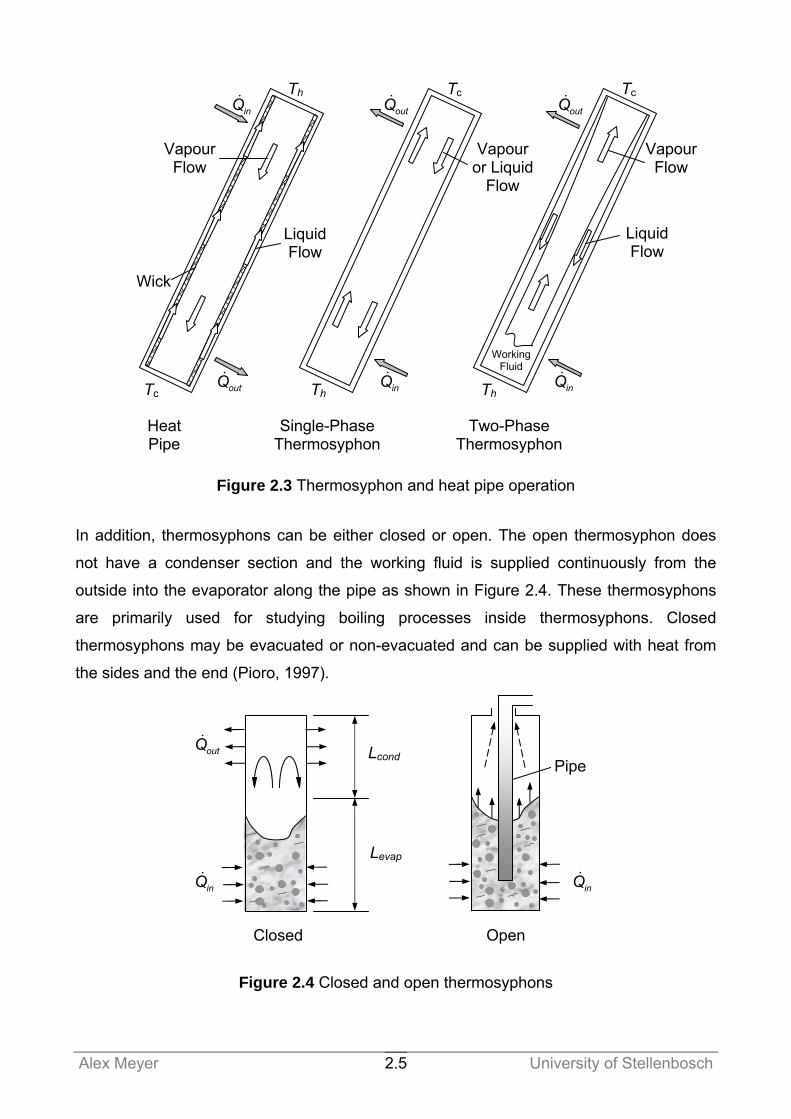
3.3 Air Drier Model ............................................................................................................................ 3.17

4 DESIGN OF A DEMONSTRATION HPHE............................................................................................ 4.1

4.1 Design Criteria and Specifications ................................................................................................ 4.1

5 EXPERIMENTAL WORK ...................................................................................................................... 5.1

5.1 Experimental Determination of the Thermosyphon Thermal Characteristics ............................... 5.1 5.1.1 Thermosyphon description........................................................................................................ 5.1 5.1.2 Thermosyphon experimental set-up ......................................................................................... 5.2

Alex Meyer University of Stellenbosch xi

5.1.3 Thermosyphon experiments undertaken .................................................................................. 5.9 5.2 Investigation into the Temperature Distribution of a HPHE ........................................................ 5.12

5.2.1 HPHE description.................................................................................................................... 5.12 5.2.2 HPHE experimental set-up ..................................................................................................... 5.13 5.2.3 HPHE experiments undertaken .............................................................................................. 5.16

5.3 Economic Analysis Experiments on a Demonstration HPHE ..................................................... 5.18 5.3.1 CFW/Yucon HPHE description ............................................................................................... 5.18 5.3.2 CFW/Yucon HPHE experimental set-up................................................................................. 5.18 5.3.3 CFW/Yucon HPHE experiments undertaken.......................................................................... 5.20

5.4 Equipment, Instrumentation and Calibrations ............................................................................. 5.22 5.4.1 Equipment and instrumentation used ..................................................................................... 5.22 5.4.2 Calibrations ............................................................................................................................. 5.23

6 RESULTS .............................................................................................................................................. 6.1

6.1 General Experimental Results ...................................................................................................... 6.1 6.1.1 Thermosyphon laboratory experiments .................................................................................... 6.1 6.1.2 Demonstration experiments on the CFW/Yucon HPHE ........................................................... 6.3

6.2 Multi-Variable linear Regression Techniques for the Heat Transfer Coefficients ......................... 6.5 6.2.1 5/8”-Thermosyphon Results: R134a......................................................................................... 6.5 6.2.2 3/4”-Thermosyphon Results: R134a......................................................................................... 6.8 6.2.3 7/8”-Thermosyphon Results: R134a......................................................................................... 6.9 6.2.4 5/4”-Thermosyphon Results: R134a....................................................................................... 6.11 6.2.5 5/8”-Thermosyphon Results: Butane ...................................................................................... 6.13 6.2.6 3/4”-Thermosyphon Results: Butane ...................................................................................... 6.15 6.2.7 7/8”-Thermosyphon Results: Butane ...................................................................................... 6.17 6.2.8 5/4”-Thermosyphon Results: Butane ...................................................................................... 6.18

6.3 Performance Correlating Equations for Thermosyphons............................................................ 6.20 6.4 Inside Temperature Distribution of a HPHE and Comparison with the Mathematical Model ..... 6.27 6.5 Demonstration Experiments on the CFW/Yucon HPHE ............................................................. 6.30

7 DISCUSSIONS AND CONCLUSIONS.................................................................................................. 7.1

8 RECOMMENDATIONS ......................................................................................................................... 8.1

9 REFERENCES....................................................................................................................................... 9.1

Alex Meyer University of Stellenbosch xii

Alex Meyer University of Stellenbosch xiii

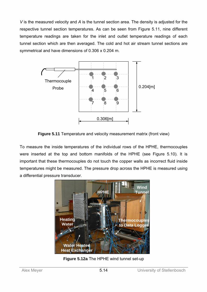
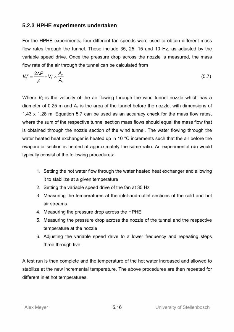
LIST OF FIGURES Figure 2.1 The Perkins Boiler (Lock, 1992) ................................................................................................... 2.1 Figure 2.2 Thermosyphon heat exchanger proposed by Gay (Lock, 1992) .................................................. 2.2 Figure 2.3 Thermosyphon and heat pipe operation....................................................................................... 2.5 Figure 2.4 Closed and open thermosyphons................................................................................................. 2.5 Figure 2.5 Loop thermosyphon operation...................................................................................................... 2.6 Figure 2.6 Heat transfer characteristics for different thermosyphons (Faghri, 1995).................................... 2.7 Figure 2.7 Typical thermosyphon chiller arrangement (Maidment and Eames, 2001)................................ 2.16 Figure 2.8 A commercial HPHE (Colmac Coil, 2000).................................................................................. 2.18 Figure 2.9 A typical air drier unit .................................................................................................................. 2.21 Figure 3.1 Thermal resistance model of a thermosyphon ............................................................................. 3.1 Figure 3.2 The tube bundle configurations, (a) Aligned, (b) Staggered ...................................................... 3.10 Figure 3.3 Plate finned tube bundle Configuration ...................................................................................... 3.13 Figure 3.4 The Plate-and-tube Control Volume, (a) Plan View, (b) Cut-away View.................................... 3.13 Figure 3.5 Plain individually finned tube configuration ................................................................................ 3.16 Figure 3.6 Plain Individually finned tube control volume ............................................................................. 3.16 Figure 3.7 The drier unit model and corresponding psychometric chart ..................................................... 3.19 Figure 4.1 Row configuration for the CFW/Yucon HPHE.............................................................................. 4.4 Figure 4.2 Flow diagram for the HPHE computer simulation program.......................................................... 4.5 Figure 5.1 The thermosyphon support structure ........................................................................................... 5.3 Figure 5.2 Thermosyphon heating and cooling water tank systems ............................................................. 5.4 Figure 5.3 Thermosyphon temperature measurement positions................................................................... 5.5 Figure 5.4 Connectivity of the charging device to the thermosyphon............................................................ 5.6 Figure 5.5 The charging device ..................................................................................................................... 5.6 Figure 5.6 Connectivity of the charging device to the thermosyphon............................................................ 5.7 Figure 5.7 The thermosyphon experimental set-up....................................................................................... 5.8 Figure 5.8a Experimental heat loss for the 5/8”-Thermosyphon ................................................................. 5.10 Figure 5.8b Experimental heat loss for the 3/4”-Thermosyphon ................................................................. 5.10 Figure 5.9 Theoretical heat losses for the thermosyphons with Tamb = 20 °C ............................................. 5.11 Figure 5.10 The HPHE used in the inside temperature distribution experiments........................................ 5.13 Figure 5.11 Temperature and velocity measurement matrix (front view) .................................................... 5.14 Figure 5.12a The HPHE wind tunnel set-up ................................................................................................ 5.14 Figure 5.12b The HPHE wind tunnel set-up (side view).............................................................................. 5.15 Figure 5.13 Theoretical heat losses for the HPHE ...................................................................................... 5.17 Figure 5.14a The HPHE installed onto the drier unit ................................................................................... 5.19 Figure 5.14b The reducer sections from the HPHE to the ducting.............................................................. 5.19 Figure 5.15 Theoretical heat losses for the demonstration HPHE .............................................................. 5.21 Figure 5.16 Calibration curve for the charge measuring device.................................................................. 5.23 Figure 6.1 Typical measured temperatures and heat transfer rates for the 3/4”-Thermosyphon.................. 6.2 Figure 6.2 Measured temperatures and heat transfer rates for the laboratory tested HPHE........................ 6.3 Figure 6.3 Readings for the industrial testing of the CFW/Yucon HPHE ...................................................... 6.4

Alex Meyer University of Stellenbosch xiv

Figure 6.4 Energy balances for the 5/8”-Thermosyphon operating with R134a charged at 50 %

liquid fill charge ratio..................................................................................................................... 6.6 Figure 6.5 Energy balances and inside evaporator and condenser heat transfer coefficients for the 5/8”-

Thermosyphon operating with R134a charged at 25 % and operating vertically and at 45° ....... 6.7 Figure 6.6 Energy balances and inside evaporator and condenser heat transfer coefficients for the 3/4”-

Thermosyphon operating with R134a charged at 50 % and operating vertically and at 45° ....... 6.9 Figure 6.7 Energy balances and inside evaporator and condenser heat transfer coefficients for the 7/8”-

Thermosyphon operating with R134a charged at 50 % and operating vertically and at 45° ..... 6.11 Figure 6.8 Energy balances and inside evaporator and condenser heat transfer coefficients for the 5/4” -

Thermosyphon operating with R134a charged at 50 % and operating vertically and at 45°. .... 6.13 Figure 6.9 Energy balances and inside evaporator and condenser heat transfer coefficients for the 5/8”-

Thermosyphon operating with Butane charged at 50 % and operating vertically and at 45° .... 6.14 Figure 6.10 Energy balances and inside evaporator and condenser heat transfer coefficients for the 3/4”-

Thermosyphon operating with Butane charged at 50 % and operating vertically and at 45° .. 6.16 Figure 6.11 Energy balances and inside evaporator and condenser heat transfer coefficients for the 7/8”-

Thermosyphon operating with Butane charged at 50 % and operating vertically and at 45° .. 6.17 Figure 6.12 Energy balances and inside evaporator and condenser heat transfer coefficients for the 5/4”-

Thermosyphon operating with Butane charged at 50 % and operating vertically and at 45° .. 6.19 Figure 6.13 Energy balances for the combined thermosyphon data sets operating vertically and inclined 6.22 Figure 6.14 Evaporator inside heat transfer coefficients for the combined thermosyphon data sets

operating vertically and inclined ............................................................................................... 6.22 Figure 6.15a Comparison between theoretically determined evaporator inside heat transfer coefficients

for vertical operation ............................................................................................................... 6.23

Figure 6.15b Comparison between theoretically determined evaporator inside heat transfer coefficients

for inclined operation .............................................................................................................. 6.23 Figure 6.16 Condenser inside heat transfer coefficients for the combined thermosyphon data sets

operating vertically and inclined ............................................................................................... 6.25 Figure 6.17a Comparison between theoretically determined condenser inside heat transfer coefficients

for vertical operation ............................................................................................................... 6.26 Figure 6.17b Comparison between theoretically determined condenser inside heat transfer coefficients

for inclined operation .............................................................................................................. 6.26 Figure 6.18 Maximum heat transfer rates for the combined thermosyphon data sets operating vertically

and inclined charged ................................................................................................................ 6.27 Figure 6.19 Inside temperature distributions of the manifolded rows of the laboratory tested HPHE

at different hot and cold air mass flow rates............................................................................. 6.28 Figure 6.20 Comparison between the evaporator and condenser heat transfer rates and the

mathematical model of the laboratory tested HPHE at different mass flow rates .................... 6.29

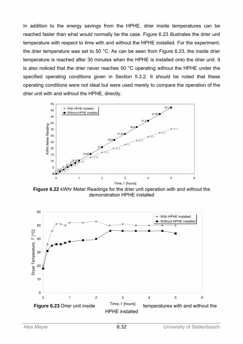
Figure 6.21 Heat recovery of the demonstration HPHE .............................................................................. 6.30 Figure 6.22 kWhr Meter Readings for the drier unit operation with and without the demonstration

HPHE installed ......................................................................................................................... 6.32 Figure 6.23 Drier unit inside temperatures with and without the HPHE installed........................................ 6.32

Alex Meyer University of Stellenbosch xv

Figure 6.24 Comparison between the mathematical model and experimentally determined heat

transfer rates using the in-field CFW/Yucon HPHE ................................................................. 6.34 Figure 7.1 Comparison between theoretically determined evaporator inside heat transfer

coefficients (smaller copy of Figure 6.15)..................................................................................... 7.4 Figure 7.2 Comparison between theoretically determined evaporator inside heat transfer

coefficients (smaller copy of Figure 6.17)..................................................................................... 7.5 Figure 7.3 Heat transfer rates for a HPHE at specified air mass flow rates compared to the

mathematical model (copy of Figure 6.20b) ................................................................................. 7.6 Figure 7.4 Comparison between the mathematical model and the experimentally determined heat

transfer rates for the CFW/Yucon HPHE (Copy of Figure 6.24) .................................................. 7.7 Figure C.1 Main window for the HPHE computer program…….……………………...………………………...C.1

Figure C.2 Physical inputs for the HPHE computer program….……………………...………………………...C.2

Figure C.3 Unfinned thermosyphon tube bank configuration for the HPHE computer program…..………...C.3

Figure C.4 Individually finned thermosyphon tube bank configuration for the HPHE computer program…..C.3

Figure C.5 Plate-and-tube bank configuration for the HPHE computer program…...………………………...C.4

Figure C.6 Error window for the HPHE computer program……………….…………...………………………...C.4

Figure C.7 Results window for the HPHE computer program….……………………...……………………......C.5

Figure C.8 Main window for the air drier computer program….……………………...………………………....C.6

Figure C.9 The physical inputs window for the air drier computer program….……………………...………...C.7

Figure C.10 Results window for the air drier computer program….…..…………………...……………………C.7

Alex Meyer University of Stellenbosch xvi

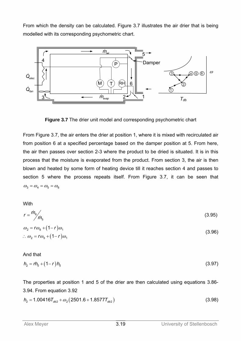
LIST OF TABLES Table 2.1 HPHE configuration (Zhang and Zhuang, 2003).......................................................................... 2.19 Table 4.1 Design specifications for the CFW/Yucon HPHE........................................................................... 4.2 Table 4.2 Design inputs for the CFW/Yucon HPHE....................................................................................... 4.3 Table 4.3 CFW/Yucon HPHE results from the computer simulation program............................................... 4.4 Table 5.1 Detailed characteristics of the experimental thermosyphons ........................................................ 5.2 Table 5.2 Characteristics of the HPHE ........................................................................................................ 5.12 Table 6.1 Average percentage differences of equation 6.34 and 6.35 with respect to correlations

presented in Section 3.1.............................................................................................................. 6.24 Table 6.2 Demonstration of the attainable heat recovery ............................................................................ 6.30 Table 6.3 Energy savings for the installed CFW/Yucon HPHE ................................................................... 6.33

Table A.1 Thermophysical properties of lighter fluid mixture……………………………………...……………..A.2

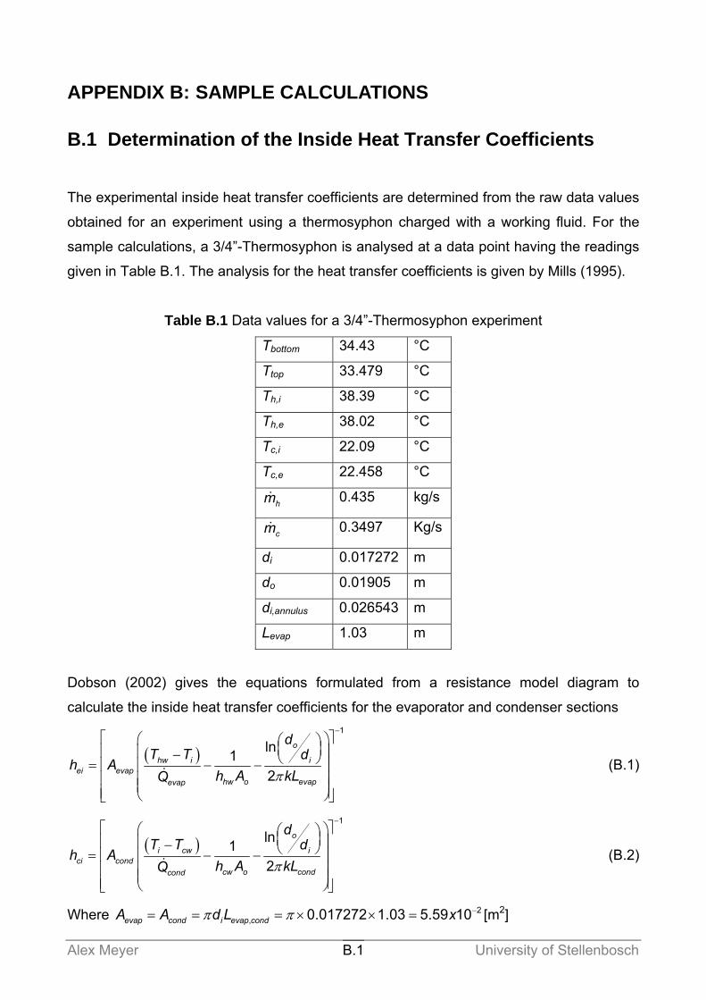
Table B.1 Data values for a 3/4"-Thermosyphon experiment……………………………………………………B.1

Table B.2 Data values for the laboratory HPHE experiments……………………………………………………B.9

Alex Meyer University of Stellenbosch xvii

NOMENCLATURE

Symbols A Area [m2]

Afr Frontal area of the tube bundle [m2]

Acva Area exposed to the air stream in control volume [m2]

Acvc Minimum free flow area of control volume [m2]

Acvf Fin surface area exposed to the air stream [m2]

Acvfr Frontal area of the control volume [m2]

Bo Bond number, ( )i l vd gσ ρ ρ−

C Wallis’ constant, 0.8

Ck Kutateledze Constant, 3.2

cp Specific heat [J/kgK]

Cw Empirically determined constant, 0.7-1

d Diameter [m]

e Fin height [m]

F Pressure factor

Fr Froude number, ( )e l fg l i l vq h d gρ ρ ρ ρ⎡ ⎤ −⎡ ⎤⎣ ⎦⎣ ⎦2

&

fφ Inclination adjustment factor

f Correction factor, friction factor

fp Enhancement factor

g Gravitational constant, 9.81 [m/s2]

G Mass velocity [kg/m2s]

h Heat transfer coefficient, Enthalpy [W/m2K], [J/kg]

hfg Latent heat of vaporization [J/kg]

hz Local heat transfer coefficient [W/m2K]

j Colburn factor

Ja Jacob number, ( )pl w sat fgc T T h−

k Thermal conductivity, Mass transfer coefficient [W/mK], [kg/sm2Pa]

Ku Kutateladze number, ( )( ) .

e v fg l v vq h gρ σ ρ ρ ρ⎡ ⎤−⎢ ⎥⎣ ⎦0 252&

L Length [m]

Lm Bubble length scale

m& Mass flow rate [kg/s]

Alex Meyer University of Stellenbosch xviii

mf Mass fraction [%]

mv Volume fraction %]

Μ Merrit number, l fg lhρ σ μ

n Wall heat flux exponent

Np Number of tubes per row

Nr Number of tube rows

uN Nusselt number

10≥udN Nusselt number for 10 or more tube bank rows

10<udN Nusselt number for fewer than 10 tube bank rows

1udN Nusselt number for one row of tubes

*uzN Local modified Nusselt number

fNμ Viscosity number

P Pressure [Pa]

Pf Fin Pitch [m]

PL Dimensionless longitudinal pitch

Pr Prandtl number

PT Dimensionless transverse pitch

Pws Saturated water vapour pressure [Pa]

q& Heat flux [W/m2]

Q& Heat transfer rate [W]

elecQ& Electrical work [W]

fanQ& Fan work [W]

lossQ& Heat losses [W]

r Recirculation ratio [%]

R2 Correlation coefficient

R Thermal resistance, Gas constant [°C/W],[kJ/(kmol.K)]

Ra Rayleigh number

Re Reynolds number

eR φ Adjusted Reynolds number

s Spacing between two fins [m]

SL Longitudinal pitch of tube bank [m]

St Transverse pitch of tube bank [m]

Alex Meyer University of Stellenbosch xix

ST Standton number

T Temperature [°C]

T Average Temperature [°C]

t Wall thickness [m]

V Velocity, Volume [m/s], [m3]

V Adjusted velocity, Average velocity [m/s]

V* Dimensionless superficial velocity

V+ Liquid fill ratio [%]

Vo Velocity of fluid in the empty cross section [m/s]

We Weber number, l lV Lρ σ2

X Dimensionless liquid pool parameter

Subscripts and superscripts a Ambient

air Dry Air

aligned Aligned

ave Average

c Condenser, Cold

cond Condenser

crit Critical

CC Combined Convection

cface Condenser face

cv Control Volume

db Dry bulb

e Evaporator, Exit

eface Evaporator face

evap Evaporator

f Liquid, fin

fo Fin outside

h Hot, Hydraulic

i Inside, inlet

in Inlet

KU Kutateledze

l Liquid, length

Alex Meyer University of Stellenbosch xx

max Maximum

NB Nucleate boiling

NC Natural convection

o Outside, outlet

s surface

sat Saturated

stag Staggered

tot Total

v Vapour

w Wall

wb Wet bulb

x Characteristic length

Greek symbols σ Area ratio, Surface tension, Stefan Boltzmann constant [N/m], [W/m2K4]

zδ Film thickness

ψ Arrangement factor, Mixing pool coefficient, Dimensionless pitch factor

φ Arrangement factor, Relative humidity, Inclination angle [°]

ρ Density [kg/m3]

Δ Difference

η Dimensionless film parameter, efficiency [%]

μ Dynamic viscosity [Ns/m2]

χ Correction factor

ω Humidity ratio at the dry bulb temperature

sω Humidity ratio at the wet bulb temperature

ν Kinematic viscosity, Specific volume [m2/s], [m3/kg]

Acronyms and Abbreviations Alt Altitude above sea level [m]

ANOVA Analysis of variance

Baro Barometric pressure [Pa]

COP Coefficient of Performance

ESDU Engineering Sciences Data Unit

Alex Meyer University of Stellenbosch xxi

HPHE Heat Pipe Heat Exchanger

in Inch = 25.4 mm

TEG Triethylene glycol

s/s Stainless Steel

Alex Meyer University of Stellenbosch 1.1

1 INTRODUCTION

Owing to ever increasing demands for global energy savings, South African Companies

are seeking to improve their international competitive edge by developing new systems

whereby wasted energy can be efficiently recovered. For this reason, heat recovery

systems are becoming increasingly important. Yucon, a large refrigeration heat exchanger

manufacturer deemed it strategically important to meet this challenge by investigating the

possibility of increasing their existing product range by adding to it the option of heat pipe

(thermosyphon) heat recovery systems. The express objective of this thesis is therefore to

meet this company’s product development requirements.

Successful implementation in the design of a heat pipe heat exchanger (HPHE) requires

detailed knowledge of the heat transfer characteristics. The development of theoretical

inside heat transfer coefficients and the maximum heat transfer rates for different

thermosyphon working fluids based on experimental data and on the physical behaviour of

the working fluid are important to determine heat transfer characteristics. Furthermore, it is

also important to investigate the performance parameters of the thermosyphons, such as

the diameter and the evaporator to condenser length ratios so that an appropriate heat

exchanger can be specified. Based on these performance parameters, a theoretical model

is developed for a thermosyphon heat recovery system whereby, by altering the

parameters, the size and predicted heat recoveries for a range of HPHE’s can be

developed.

HPHE’s are used in many countries world-wide in a variety of applications. However, they

have as yet not been accepted by the South African market. Continental Fan Works

(CFW), a design and manufacture company specialising in drying systems and other air

handling products were willing provide an opportunity to demonstrate the performance of

such a HPHE. The objective is therefore to verify the economic viability of using such a

heat recovery system in a practical industrial application. The economic evaluation of the

demonstration unit is therefore considered and includes factors such as the initial costs,

running costs and the energy savings of the HPHE.

A literature survey is conducted to give insight into heat pipes (thermosyphons) and

HPHEs. The performance parameters and the characteristics that influence the


performance of thermosyphons were specifically studied. This survey is located in Section

2. The theory from which the theoretical model is developed is located in Section 3.

Section 4 describes the design specifications for the demonstration HPHE and presents

the results from the computer simulation program. Section 5 discusses the experimental

design and set-ups and experimental procedures followed whilst Section 6 presents the

results from the experimental work. The discussions and conclusions pertaining to the

results in Section 6 are presented in Section 7 with recommendations given in Section 8.


Expansion Tube

Heat

Interceptor

Evaporator

Condenser

2 LITERATURE STUDY

The modern day development of heat pipes and thermosyphons began with a journal entry

by George Grover on July 24, 1963, in which a device capable of heat transfer via capillary

movement of fluids was suggested. This device has since found uses in a variety of

applications and popularity is ever-increasing worldwide. The historical development and

essential characteristics of thermosyphons and heat pipes will be considered in this

literature study.

2.1 Historical Development of Heat Pipes

The heat pipe concept was first introduced in the 1800’s by patents formulated by A. M.

Perkins and his son, J. Perkins. These men developed what is known as the Perkins tube,

a device that works on the principle of using either single or two-phase processes to

transfer heat from a furnace to a boiler. This device consists of a tube with an airtight

space partially filled with water as the working fluid. In the space, boiling with the formation

of vapour and liquid, condensation, and free convection heat and mass transfer between

the boiling and condensation regions occurs. The earliest applications of these tubes were

in locomotive boilers and in locomotive fire box super heaters. Figure 2.1 illustrates the

Perkins boiler. In the Perkins boiler, one end of each tube projects downwards into the fire

and the other part extends up into the water of the boiler. Any additional heat applied

thereto will quickly rise to the upper parts of the tubes and be given off to the surrounding

water contained in the boiler (Pioro, 1997).

Figure 2.1 The Perkins Boiler (Lock, 1992)


Cold Air

Hot Air

Separator Plate

Condenser

Finned Tubes

Evaporator

At a time when high pressure boilers were still experimental and their operation was

plagued by scaling and fouling problems, the system proposed by Perkins represented

excellence in design as tests verified that there was no leakage and no deposits of any

kind occurring within the tube. In the patent taken out by Perkins’ in 1892, mention is made

of applications of the Perkins tube to waste heat recovery, where the heat is recovered

from the exhaust gases from blast furnaces and other similar apparatus, and used to

preheat incoming air.

Perkins’ patents however neglected to include the use of external fins on the tubes to

improve the tube-to-gas heat transfer. Gay introduced the fin concept and took out a

patent in 1929, in which a number of finned Perkins tubes were situated vertically with the

evaporator section below the condenser section (Dunn, 1994). A plate then sealed the

passage between the exhaust and inlet air ducts as illustrated in Figure 2.2. It was this

setup, which, with the introduction of capillary forces, laid the groundwork in the

development of what is today known as a heat pipe (Peterson, 1994).

Figure 2.2 Thermosyphon heat exchanger proposed by Gay (Lock, 1992)

Following the groundwork by Gay, Gaugler then envisioned a device which would

evaporate a liquid at a point above the place where condensation would occur without

requiring any additional work to move the liquid to the higher elevation and it was this idea,

which led to the introduction of the heat pipe concept.


A heat pipe consists of a sealed pipe lined with a wicking structure in which a small

amount of working fluid is present. A heat pipe can further be divided into two sections,

namely, the evaporator or heat addition and condenser or heat rejection sections. When

heat is added to the evaporator region, the working fluid present in the wicking structure is

heated until it vaporizes. The pressure differences between the two regions then cause the

vapour to flow to the cooler condenser section. The vapour then condenses in this section

and gives up its latent heat of vaporization. The capillary forces in the wicking structure

then pump the liquid back to the evaporator. Gaugler later introduced this principle of using

a wicking structure to allow for large heat transfers with minimal temperature drops for

applications in refrigeration engineering. However, the heat pipe proposed by Gaugler was

not developed beyond the patent stage (Dunn, 1994).

In 1962 the heat pipe idea was resurrected by Trefethen in connection with high-

temperature space power systems (Ivanovskii, 1982). Serious development then started in

1963 when the heat pipe was independently reinvented by Grover at Los Alamos National

Laboratory in New Mexico. Grover demonstrated the heat pipes effectiveness as a high

performance heat transmission device. Cotter’s publication in 1965, in which the

theoretical results and design tools were reported, is however responsible for the

recognition of the heat pipe. Following this publication, research began worldwide (Faghri,

1995).

In 1968 Nozu (1969) described an air heater using a bundle of finned heat pipes. This later

became known as a heat pipe heat exchanger (HPHE) and was of significant importance

owing to the increasing interest in energy conservation and environmental protection

world-wide. The exchanger could then be used to recover heat from hot exhaust gases

and be applied in industrial and domestic air conditioning (Dunn, 1994). For the

aforementioned reasons, these heat exchangers are the most widely known applications

of heat pipes since the early 1990’s.


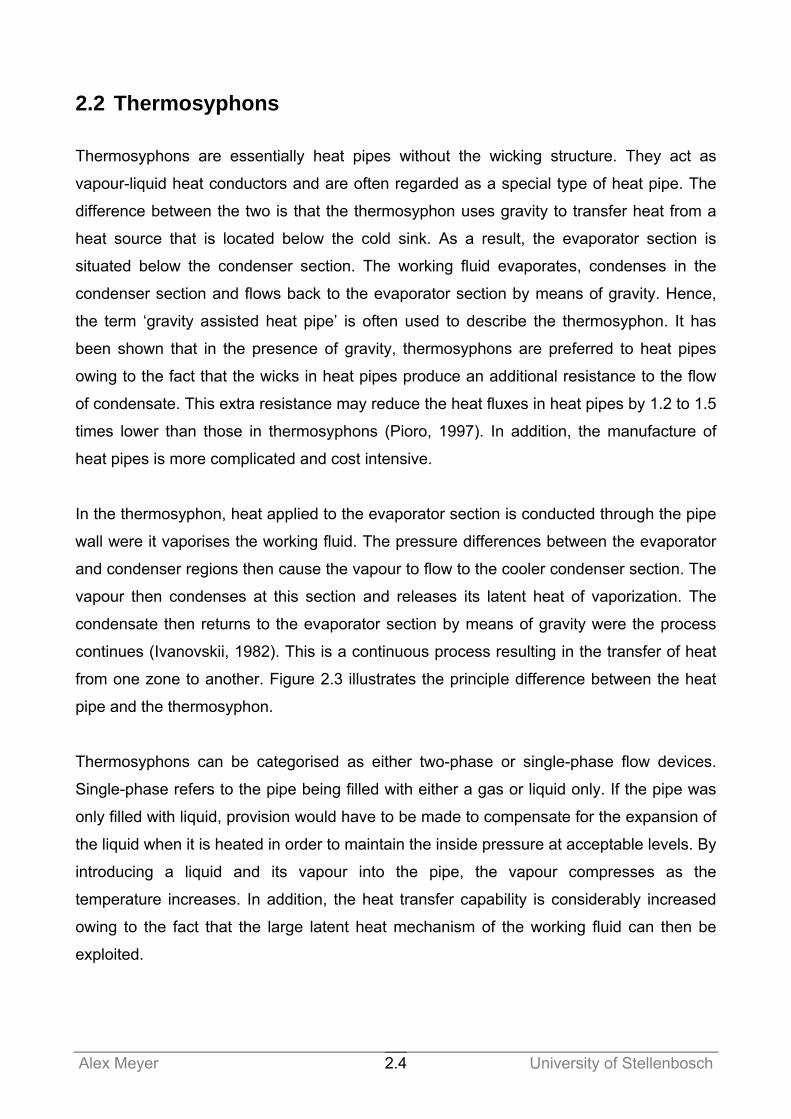
2.2 Thermosyphons

Thermosyphons are essentially heat pipes without the wicking structure. They act as

vapour-liquid heat conductors and are often regarded as a special type of heat pipe. The

difference between the two is that the thermosyphon uses gravity to transfer heat from a

heat source that is located below the cold sink. As a result, the evaporator section is

situated below the condenser section. The working fluid evaporates, condenses in the

condenser section and flows back to the evaporator section by means of gravity. Hence,

the term ‘gravity assisted heat pipe’ is often used to describe the thermosyphon. It has

been shown that in the presence of gravity, thermosyphons are preferred to heat pipes

owing to the fact that the wicks in heat pipes produce an additional resistance to the flow

of condensate. This extra resistance may reduce the heat fluxes in heat pipes by 1.2 to 1.5

times lower than those in thermosyphons (Pioro, 1997). In addition, the manufacture of

heat pipes is more complicated and cost intensive.

In the thermosyphon, heat applied to the evaporator section is conducted through the pipe

wall were it vaporises the working fluid. The pressure differences between the evaporator

and condenser regions then cause the vapour to flow to the cooler condenser section. The

vapour then condenses at this section and releases its latent heat of vaporization. The

condensate then returns to the evaporator section by means of gravity were the process

continues (Ivanovskii, 1982). This is a continuous process resulting in the transfer of heat

from one zone to another. Figure 2.3 illustrates the principle difference between the heat

pipe and the thermosyphon.

Thermosyphons can be categorised as either two-phase or single-phase flow devices.

Single-phase refers to the pipe being filled with either a gas or liquid only. If the pipe was

only filled with liquid, provision would have to be made to compensate for the expansion of

the liquid when it is heated in order to maintain the inside pressure at acceptable levels. By

introducing a liquid and its vapour into the pipe, the vapour compresses as the

temperature increases. In addition, the heat transfer capability is considerably increased

owing to the fact that the large latent heat mechanism of the working fluid can then be

exploited.


Figure 2.3 Thermosyphon and heat pipe operation

In addition, thermosyphons can be either closed or open. The open thermosyphon does

not have a condenser section and the working fluid is supplied continuously from the

outside into the evaporator along the pipe as shown in Figure 2.4. These thermosyphons

are primarily used for studying boiling processes inside thermosyphons. Closed

thermosyphons may be evacuated or non-evacuated and can be supplied with heat from

the sides and the end (Pioro, 1997).

Figure 2.4 Closed and open thermosyphons

Lcond

Levap

Closed Open

inQ&

outQ&

inQ&

Pipe

Th Tc Tc

Tc Th Th

inQ&

inQ& inQ&

outQ& outQ&

outQ&

Two-Phase Thermosyphon

Heat Pipe

Single-Phase Thermosyphon

Liquid Flow

Vapour Flow

Vapour Flow

Vapour or Liquid

Flow

Liquid Flow

Working Fluid

Wick


Liquid Flow

Vapour Flow Applied

Heat Source

Vapour Line

Liquid Line

Evaporator Condenser

Aerosyphons are also a variety of thermosyphons in which the heat flux is transmitted by

forced convection of the liquid. This involves passing a saturated gas through the liquid,

causing the liquid to bubble intensively helping stir the liquid. However, this type of

thermosyphon has as yet no applications and is primarily used to investigate boiling heat

transfer since the boiling process is simulated rather well (Lock, 1992).

When heat is applied to the evaporator, in a loop arrangement, the liquid evaporates and

flows through the vapour transport line to the condenser zone, where heat is removed.

This is then known as a loop thermosyphon illustrated in Figure 2.5. The liquid

subsequently returns to the evaporator via a sub cooled liquid return line, which collapses

any remaining vapour bubbles. Consequently, smooth wall tubing can be employed in the

construction of the vapour and liquid transport lines as well as in the condenser zone as no

wicking structure is needed. This avoids the liquid flow losses that would be apparent in a

conventional heat pipe (Yun and Kroliczek, 2002).

Figure 2.5 Loop thermosyphon operation

2.2.1 Thermosyphon characteristics

One of the main reasons why thermosyphons are becoming ever more popular is the fact

that they have a very high effective thermal conductance. As an example, these pipes are

able to conduct up to 1000 times more heat, under favourable conditions, than copper in

the same space and time (Russwurm, Part 1, 1980). Faghri (1995) illustrated this by

comparing a copper rod of 25.4 mm OD and different thermosyphons. Figure 2.6 illustrates

the heat transfer characteristics.


0

500

1000

1500

2000

2500

3000

3500

4000

0 10 20 30 40 50 60 70 80 90

Mean Temperature Difference Across the Heat Pipe [°C]

Hea

t Tra

nsfe

r Rat

e [W

]25.4 mm OD Copper Rod 12.7 mm OD Thermosyphon

15.9 mm OD Thermosyphon 19.1 mm OD Thermosyphon

25.4 mm OD Heat Pipe 25.4 mm OD Thermosyphon

Figure 2.6 Heat transfer characteristics for different thermosyphons (Faghri, 1995)

Thermosyphons also have the ability to act as a thermal flux transformer where energy

can be added at a high heat flux rate to the pipe over a small surface area and removed

over a larger surface area at a lower heat flux, or vice versa. In addition, thermal flux

transformation ratios of 15 to 1 can be achieved using thermosyphons (Faghri, 1995). By

determining the conditions at the condenser, the thermosyphon can be designed to keep a

nearly constant temperature at the evaporator section even though the rate of heat input to

the evaporator varies. Another important characteristic of the thermosyphon is the fact that

as it is a closed system, the thermosyphon can operate over lengthy periods without

maintenance and is self contained.

When evaluating the thermal characteristics of the thermosyphon, it is important to

consider the evaporator and condenser heat transfer coefficients. These heat transfer

coefficients can be determined either experimentally or modelled mathematically using

computational fluid dynamics (CFD). However, the use of CFD to date is limited and the

results not entirely believable as many assumptions are used in evaluating the boundary

conditions of the thermosyphon. The chaotic behaviour of the working fluid inside the

thermosyphon also makes this method of determining the heat transfer coefficiients very

difficult. Hence, most researchers use experiments to determine the heat transfer

capabilities of various fluids. The evaporator and condenser heat transfer coefficients will

now be discussed with detailed correlations given in Section 3.1.


The inside evaporation heat transfer coefficient

The evaporation heat transfer coefficient is an important variable in the design of any

thermosyphon. The falling film of liquid that is established in the condenser section

persists into the evaporator section. At the upper part of the evaporator, the liquid film is

sub-cooled. As the liquid falls, it reaches its saturation temperature and finally becomes

superheated. Evaporation and nucleate boiling may both occur in the falling film and in the

liquid pool situated at the bottom of the evaporator (Faghri, 1995).

The three mechanisms of boiling are nucleate, convective and film boiling and it is general

practice to accept nucleate boiling inside thermosyphons, where vapour bubbles start to

grow from nucleation sites. As the heat transfer coefficient is high in nucleate boiling, it is

therefore a very efficient mode of heat transfer. As boiling is complex and difficult to model

theoretically, the heat transfer coefficients are generally given by experimentally

determined correlations. Whalley (1987) provides correlations for calculating the boiling

heat transfer coefficient based on the Chen correlation. Pioro (1997) also provides many

correlations for evaporative heat transfer coefficients for different configurations and

working fluids. However, care must be exercised as they give wildly differing results.

Dobson and Pakkies (2002) developed inside evaporator heat transfer coefficients for a

R134a charged thermosyphon. A liquid fill charge ratio of 50 % was used and the tests

were conducted for varying orientation angles. Their results showed that the heat transfer

coefficients differed significantly for a vertical and an inclined thermosyphon. However,

once inclined, the heat transfer coefficients did not vary significantly for inclination angles

between 20 and 70˚. They also showed that the maximum heat transfer rate when inclined

at 45˚ is approximately 40 % higher than that of the vertical position.

Dobson and Kröger (1999) developed inside heat transfer coefficients for an ammonia-

charged two-phase thermosyphon. Their results showed that their predicted heat transfer

correlation was within 10 % of the experimental values. They also showed that existing

pool boiling heat transfer coefficient correlations for ammonia under-estimated by on

average of 57 % the experimentally determined values for a vertically orientated

thermosyphon.


The inside condensation heat transfer coefficient

The vapour generated in the evaporator section rises up to the condenser section, where it

condenses and returns to the evaporator as a falling liquid film. This condensation can

occur either as filmwise condensation were the condensate forms a continuous film or as

dropwise condensation (which does not wet the surface well). The latter is difficult to

obtain and hence filmwise condensation is generally modelled as condensation inside a

vertical tube using the Nusselt theory (Whalley, 1987). The continuity, momentum and

energy equations can be solved for a liquid film control volume.

The result of combining the continuity, momentum and energy equations yields the local

heat transfer coefficient

( )l l v fg lz

l sat

gh kh

T zρ ρ ρ

μ⎡ ⎤−

= ⎢ ⎥Δ⎢ ⎥⎣ ⎦

0.253

4 (2.1)

However, the average heat transfer coefficient is normally of more importance than the

local heat transfer coefficient and is given by

( )l l v fg l

l sat

gh kh

T L

0.25383

ρ ρ ρμ

⎡ ⎤−= ⎢ ⎥

Δ⎢ ⎥⎣ ⎦ (2.2)

Pan (2001) investigated the condensation heat transfer model by considering the

interfacial shear due to mass transfer and interfacial velocity. Pan’s model predictions

differed significantly from the Nusselt solutions. This emphasised the significance of the

interfacial shear on the condensation inside the thermosyphon as the interfacial shear due

to the counter-current liquid and vapour flow obstructs the flow of the film.

2.2.2 Performance limitations and critical parameters of thermosyphons

Some of the limitations and factors affecting thermosyphon performance include flooding,

entrainment and dry-out and boiling limitations. These factors are discussed in this section.

The flooding and entrainment limits

Viscous shear interfacial forces arise when the relative velocity between the liquid and

vapour increases and it is these forces that prevent the return of the liquid from the


condenser to the evaporator. The thermosyphon is then said to have reached flooding

when all the liquid, just some of the liquid or all of the liquid just some of the time is

prevented from returning to the evaporator. When additional heat is applied, the vapour

velocity will increase, resulting in the liquid-vapour interface becoming unstable and

unsteady. This then results in the liquid viscous forces being greater than the surface

tension forces resulting in liquid droplets being entrained in the vapour region of the

condenser section. This limitation is then known as the entrainment limit.

Wallis (1969) and Kutateladze (1972) formulated correlations for predicting the flooding

limit of two-phase flows. The Wallis correlation however falls short as the effect of surface

tension is not taken into account (Faghri, 1995). The Wallis equation is as follows:

l vV V C1 1* *2 2+ = (2.3)

Were Vl* is a dimensionless liquid superficial velocity given by

( )l l

l

l v

VVgd

12

*12

ρ

ρ ρ=⎡ ⎤−⎣ ⎦

(2.4)

And Vv* is a dimensionless vapour superficial velocity given by

( )v v

v

l v

VVgd

12

*12

ρ

ρ ρ=⎡ ⎤−⎣ ⎦

(2.5)

And C is a constant with a value of about 0.8.

The Kutateladze number correlation, on the other hand, includes the effect of the surface

tension but does not include the effect of the pipe diameter. The Kutateladze numbers for

the vapour and liquid are as follows:

( )v v

v

l v

VKg

12

14

ρ

σ ρ ρ=⎡ ⎤−⎣ ⎦

(2.6)

( )l l

l

l v

VKg

12

14

ρ

σ ρ ρ=⎡ ⎤−⎣ ⎦

(2.7)


The most commonly quoted correlation of this type is that Kv = 3.2 derived by Pushkina

and Sorokin (1969). Whaley (1987) suggests that the Wallis-type correlation be used if the

tube diameter is small (<50 mm) and that the Pushkina and Sorokin correlation be used if

the tube diameter is large (>50 mm).

Faghri et al. (Faghri, 1995) improved the existing semi-empirical correlations by including

the effects of diameter, surface tension and working fluid properties. The following

correlation was formulated for the maximum heat transfer rate:

( )fg l v v lQ Kh A gσ ρ ρ ρ ρ−− −⎡ ⎤⎡ ⎤= − +⎣ ⎦ ⎢ ⎥⎣ ⎦

21 1 14 4 4max& (2.8)

Were K is a Kutateledze number defined by

l

v

K Bo0.14

12 4tanhρρ

⎛ ⎞= ⎜ ⎟⎝ ⎠

(2.9)

And Bo is the Bond number defined by

( )k

w l v

CBoC g

σρ ρ

⎡ ⎤⎛ ⎞= ⎢ ⎥⎜ ⎟ −⎢ ⎥⎝ ⎠ ⎣ ⎦

14 2

; kC = 3.2 (2.10)

With Ck, a constant defined by Kutateladze and Cw, an empirically determined constant

ranging between 0.7 and 1 for various fluids.

The influence of filling plays an important role in the flooding limit. It can be summarised as

follows: for small charges, the heat transfer limit increases as some power of the filling

ratio; for large charges, the heat transfer limit remains constant (Lock, 1992). The liquid fill

charge ratio is defined by the ratio of the volume of the liquid phase of the fluid under initial

conditions to the inner volume of the thermosyphon or the evaporator volume. It is

important to make the distinction between the fill-charge ratio with respect to the entire

volume of the thermosyphon or just the evaporator volume when designing the

thermosyphon as this can result in improper operation. It is recommended that in actual

use, the quantity of working fluid charge should be between 30-33 % of the total volume of

the thermosyphon. If however, the length of the condenser is longer than the evaporator,

the ratio of the volume of liquid to the evaporator volume should be 50 % (Pioro, 1997).


Park et al. (2002) investigated the effects of the fill charge ratio for a two-phase closed

thermosyphon. For the tests, a copper container with FC-72 as working fluid was used.

The experiments were performed in the range of 50-600 W heat flow rate and 10-70 % fill

charge ratio. The results showed that the heat transfer coefficient of the evaporator to the

fill charge ratio were nearly negligible. However, at the condenser, the heat transfer

coefficients showed some enhancements with the increase of fill charge ratio. However, no

optimum fill charge ratio is given.

The dry-out limitation

When the liquid charge volume and the radial evaporator heat flux are very small, the dry-

out limitation is reached at the bottom of the evaporator. The falling condensate persists

into the evaporator section with its thickness approaching zero at the bottom. As a result,

the entire amount of working fluid is circulated either as a falling film or as a vapour. A pool

of liquid at the bottom of the evaporator is therefore not present and if the heat flux is

increased, dry-out of the film will start from the bottom upwards, effectively shortening the

evaporation area. The evaporator wall temperature will then increase steadily but the heat

transfer rate will not (Faghri, 1995).

The boiling limitation

When the fill volume of the working fluid is large and the radial heat flux in the evaporator

section is high, boiling limitation is achieved. As the heat flux is increased, nucleate boiling

occurs in the evaporator. At the critical heat flux, the vapour bubbles coalesce near the

pipe wall, which essentially prevents the liquid from touching the wall. The wall

temperature then increases rapidly to compensate for the loss in heat flux, since the gas

bubbles allow for an increase in thermal resistance for heat flow into the liquid (Faghri,

1995).

Other Literature regarding performance limitations and critical parameters of

thermosyphons

The effect of the thermosyphon geometry also plays a critical role on the value of the

limiting heat flux. Some researchers report that only the diameter affects the maximum

heat transfer (Qmax& ) whereas others report that only the evaporator length is the


determining factor. Recent studies show however, that both affect the value of Qmax& .

Experimental data has shown that with decreasing di/Levap, the value of Qmax& is

increasingly affected by the interaction between the counter directed vapour and liquid

flows. Whereas the dimensions of the evaporator exert a significant effect on Qmax& the

dimensions of the adiabatic length (section of the thermosyphon between the evaporator

and condenser) and condenser do not have a significant effect. The geometric dimensions

of the condenser may however affect the limiting heat transmitting capability of the

thermosyphon indirectly owing to the fact that the pressure in the thermosyphon depends

on the condenser dimensions and on the conditions of its cooling (Pioro, 1997).

Abou-Ziyan et al. (2001) investigated the performance of a thermosyphon with water and

R134a as working fluids. For their tests, a copper pipe of OD 25 (ID 23) mm and 900 mm

total length was used. The effect of the adiabatic length (a separator section between the

evaporator and condenser section) was investigated. Their results showed that for their

thermosyphon, the capability of the thermosyphon to transfer large amounts of heat is

enhanced as the adiabatic length increases. They also investigated the effect of the liquid

fill charge ratio. They concluded that the largest heat transport is obtained for a fill charge

ratio of 50 %.

When selecting the working fluid, the first consideration is temperature (and hence the

pressure of the vapour). The temperature is important as to ensure that the working fluid is

stable and will not break down into its separate chemical components. The pressure is

important to ensure that the thermosyphon does not leak. It is also important for the

working fluid to have a high latent heat of vaporisation in order to transfer large amounts of

heat with low vapour flow rates. The critical parameters of the working fluid should also be

higher than the operating temperature of the thermosyphon. It has been shown that water

is a good working fluid. It permits the transformation of more heat than all the other known

working fluids, is inexpensive, readily available and is fire and explosion safe. However, it

also has the ability to react with some substances, e.g. stainless steel (Pioro, 1997).

Payakaruk et al. (2000) investigated the heat transfer characteristics of an inclined

thermosyphon. In their experiments, copper thermosyphons with ID’s of 7.5, 11.1 and

25.3 mm were employed with R22, R123, R134a, ethanol, and water as the working fluids.

The inclination angle was varied from the horizontal axis and the vapour temperature


ranged from 0 to 30 ˚C. Their results showed that the working fluid increased the heat

transfer rate at inclination angles of 20 to 70˚ and that the lower the latent heat of

vaporization of the fluid, the higher the heat transfer rate.

Dobson and Kroger (2000) investigated the thermal characteristics of an ammonia

charged two-phase closed thermosyphon. For their setup, the thermosyphon consisted of

a 6.2 m long by 31.9 mm inside diameter stainless steel pipe. The heating water from the

hot water supply was increased from room temperature to a maximum of 80 ˚C and the

cooling water varied between 10 and 20 ˚C. Their results showed that the inside heat

transfer coefficients are complicated functions of the heat flux, temperature, liquid fill

charge ratio, orientation and the evaporator and condenser lengths.

Nuntaphan et al. (2002) investigated the heat transport in a thermosyphon air preheater at

high temperatures with a binary working fluid. For the test case, an ID 9.5 mm copper pipe

with a wall thickness of 1 mm was used as the thermosyphon. The lengths of the

evaporator, condenser and adiabatic sections were 400, 400 and 200 mm. The working

fluid was water and the binary fluid that was added to the water was triethylene glycol

(TEG). The filling ratio was 50 % of the evaporator volume. Their results showed that using

TEG-water mixture, the critical limit due to flooding inside the thermosyphon could be

extended and that the limit is directly proportional to the amount of TEG in the mixture. The

tests also showed that with a suitable mixture of TEG-water, the performance of the

preheater can be increased by 30-80 % for a parallel flow and 60-115 % for a counter flow

air preheater compared to pure TEG.

2.2.3 Applications

As heat pipes can be used over a very wide temperature range, from cryogenic

temperatures (starting from -272 °C) to the high temperatures (2200-2700 °C), their

applications cover a wide spectrum. They can be used in underground cool rooms, for

aircraft temperature control and in spacecraft, to name but a few. The primary applications

can however, be divided into two main categories: heat transfer from a heat source to a

sink and temperature equalization control. Some uses of heat pipes (specifically

thermosyphons) will now be discussed.


Dehumidification and air conditioning:

In an air conditioning system, the heat removed in cooling the incoming air to the

thermosyphon can be recovered and used to reheat air. This increases the moisture

removal capacity of the air conditioning system. The thermosyphon then recovers the

energy in the hot humid air and uses it to re-heat the cold, dehumidified air. This saves in

energy expenditure and also in a smaller cooling coil resulting in a more cost-effective

system (Dobson, 1999). Wu et al. (1997) showed that for a specific test condition, the

cooling capability of a system can be enhanced by 20 to 32.7 % using a HPHE.

Electric power generation:

Electric power is generally produced by means of the Rankine cycle. In this cycle, fossil

fuel is converted into high pressure vapour in a boiler. The vapour moves through the

turbine where its energy is converted into rotational power. This causes rotation of the

turbine’s shaft which in turn drives an electrical generator. Akbarzadeh et al. (2001)

investigated the concept of a heat pipe turbine or thermosyphon Rankine engine for power

generation using solar, geothermal or other available low grade heat sources. The basis of

the engine is the thermosyphon cycle, which is modified to incorporate a turbine in the

adiabatic region. The basic configuration is a closed vertical cylinder functioning as an

evaporator, an insulated section and a condenser. The turbine is placed in the upper end

between the insulated section and the condenser section, and a plate is installed to

separate the high pressure region from the low pressure region in the condenser. The

mechanical energy developed by the turbine can be converted to electrical energy by

direct coupling to an electrical generator. Results showed that an electrical power output of

100 W could be achieved with a heat input of 10 kW and 6000 rpm.

Heat recovery systems:

As heat pipes are characterised by their high heat transfer capabilities and no external

power requirements, they are being used in various heat exchangers for various

applications. Advantages of these exchangers compared to the standard heat exchangers

is the fact that they are nearly isothermal and can be built with better seals to reduce

leakage. Cost savings are also evident with these exchangers as they are smaller and no

power requirements are needed. HPHE’s will be discussed in Section 2.3.


Compressor

Chiller

Condenser Condenser

Compressor Chiller

Four Port Valve

Other Applications:

In a summary of the proceedings of the UK Institute of Refrigeration in 1998/1999 by

Maidment and Eames (2001), thermosyphon developments for air conditioning are

presented. A thermosyphon chiller consisting of a compressor, chiller, condenser and a

four port valve is used to describe the free cooling capability of a thermosyphon. In this

set-up, when the compressor is turned off the system operates by circulating refrigerant to

the condenser without the use of the compressor but by means of the pressure difference

produced by the temperature difference between the cooled water and the ambient air. It is

shown that average coefficients of performance (COP) of between 10 and 13 can be

obtained. In the report, mention is made of the first ammonia charged thermosyphon chiller

installation in the UK. The 20 year life cycle cost of ownership for this system was

estimated to be 55 % of that for an alternative system and COP’s of between 8.5 and 14

were obtained. Figure 2.7 illustrates a typical thermosyphon chiller unit.

Figure 2.7 Typical thermosyphon chiller arrangement (Maidment and Eames, 2001)

Pan et al. (2002) investigated the applications on freezing expansions of soil restrained

two-phase closed thermosyphons. In cold regions, foundations of buildings are often

deformed and damaged due to the freezing expansion of the soil in winter. One of the

ways to prevent this damage is to make use of thermosyphons in which the evaporator

section is buried in the soil and the condenser section is exposed to the air. When the air

temperature is below the soil temperature, the evaporation-condensation cycle inside the

thermosyphon starts and the thermal energy in the soil is then transferred into the

environment and the soil temperature decreases. The soil remains frozen and the number

of thaw cycles are reduced.


2.3 Heat Pipe Heat Exchangers (HPHEs)

Waste heat is heat which is generated in a process but then rejected to the environment

even though it could still be reused for some useful or economic purpose. Sources of

waste heat can be divided according to three temperature ranges. High temperature range

(>650 °C), medium temperature range (230-650 °C) and low temperature range (<230 °C).

Heat exchangers are devices generally used to recover the waste heat and depending on

the configuration of the exchanger, can be used in all three temperature ranges (Goldstick,

1983).

The flow configuration for heat exchangers can be classified as single stream, parallel-flow

two-stream, counterflow two-stream or cross flow two-stream. A single stream exchanger

is one in which the temperature of only one fluid changes and the direction in which the

fluid flows is immaterial. Condensers and boilers are examples. In the parallel-flow two-

stream exchanger, the two fluids flow parallel to each other in the same direction.

Examples are the shell and tube exchanger which is generally used for liquids and for high

pressures. Fluids flow parallel to each other in opposite directions in a counterflow two-

stream exchanger. The effectiveness is higher than that of a parallel flow exchanger and

examples are feed water preheaters for boilers and oil coolers for aircrafts. In the cross

flow two-stream exchanger, the two streams flow at right angles to each other. The hot

stream may flow inside tubes arranged in a bank in a direction generally at right angles to

the tubes. Either one or both of the streams may be unmixed (Mills, 1995).

Heat exchangers can also be classified as either regenerators or recuperators. In

regenerators, heat is alternatively removed from the high temperature fluid and transferred

to the low temperature fluid via a heat source. The energy transfer is dependant on the

physical properties of the fluids and heat transfer surface as well as the flow situation of

the two fluids. In recuperative heat exchangers, the high and low temperature fluids do not

come into direct contact with each other but are separated by a barrier. The heat is

transferred from the high temperature source through the wall into the lower temperature

fluid by conduction through the supporting wall.

HPHEs are liquid-coupled indirect transfer type heat exchangers except that the HPHE

employs heat pipes or thermosyphons as the major heat transfer mechanism from the

high-temperature to the low-temperature fluid and do not require an external pump to


circulate the coupling fluid. They can be used for gas-to-gas, gas-to-liquid and liquid-to-

liquid heat exchange. For the HPHE, the evaporator section of the thermosyphon is

situated in the hot stream and the condenser section is situated in the cold stream. Heat

transfer is aided by the addition of fins to increase the surface area available for

convective heat transfer (Faghri, 1995). Figure 2.8 illustrates a commercial HPHE.

Figure 2.8 A commercial HPHE (Colmac Coil, 2000)

The use of heat pipes or thermosyphons in the exchanger configuration is ever-increasing

in popularity and is attributed to the following advantages:

Thermosyphons have no moving parts and auxiliary working fluid power

requirements are not needed.

The hot and cold streams of the HPHE can be completely isolated preventing cross-

contamination of the fluids.

The rate of heat transferred can be increased by adjusting the tilt angle.

HPHE are redundant in design. If one thermosyphon fails the heat exchanger is still

operational.

HPHE have the ability to operate as thermal transformers. By altering the relative

lengths of the evaporator and condenser sections the temperature at which the heat

is transferred can be selected or adjusted.

Commercial production of HPHEs began in the mid-1970s and have since found many

applications in industry. These applications can be divided into three main categories

(Noie-Baghban and Majideian, 2000):

Heat recovery in air conditioning devices.

The HPHE is installed in the ventilation system and recovers heat from the stale

outgoing air and transfers it to the fresh incoming air. For these HPHE’s, high heat


transfer coefficients and heat transfer surface areas are needed to offset the

relatively low temperature difference between the two fluid streams.

Heat recovery from the process exhaust streams to preheat air for space heating.

The temperatures encountered here are generally higher than those in the HVAC

applications. The temperature difference is also much higher. The thermosyphons

are generally constructed of copper for lower temperature exhaust streams and

carbon-steel for higher temperature applications.

Heat recovery from the process exhaust streams to re-use in the process.

The most severe applications are in the exhaust waste heat recovery for re-use in

the process industries. Examples of such application include air driers and ovens.

Temperatures up to 400 ˚C are common to exhaust streams of industrial processes.

Zhang and Zhuang (2003) investigated the use of heat pipe gas-gas heat exchangers and

heat pipe air preheaters. They investigated 20 different structure types of 26-32 mm in

diameter and 1.2-2 m in length under 300 different operating conditions. The following

table illustrates a typical air preheater that was investigated. The heat recovery of

11970 kW illustrates the economic efficiency and the important role that such a heat

exchanger can play in the energy-saving transformation in large plants.

Table 2.1 HPHE configuration (Zhang and Zhuang, 2003)

Pipe size [mm] OD 51 t=4.5, L = 6000, 1914 pieces

Heat Exchanger size [m] Height 6.4, Length 2.4,

Inlet width 13.7, Outlet width 10.37

Flue gas Air

Flow rate [Nm3/h] 238000 195860

Inlet temp [˚C] 297.7 54.8

Outlet Temp [˚C] 171.2 228.7

Pressure Drop [Pa] 580 280

Heat Recovery [kW] 11970

Lukitobudi et al. (1995) investigated the design, construction and testing of a

thermosyphon heat exchanger for medium temperature heat recovery. For the tests, water

was used as the working fluid. Copper pipes of OD 15.88 mm were used and evaporator,

condenser and adiabatic lengths were 300, 300 and 150 mm respectively. From the study,


effectiveness for the thermosyphon heat exchanger was evaluated and a maximum

effectiveness formulated. The results of the study showed that by using a finned copper

thermosyphon heat exchanger as apposed to a finned steel thermosyphon heat pipe

exchanger, effectiveness values ranging between 17.8 - 63 % could be obtained instead of

6.2 - 48.5 %.

Yang et al. (2003) demonstrated the use of a gravity assisted heat pipe heat exchanger for

heat recovery of the exhaust gas of an automobile. In cold areas, the heat of the

automotive exhaust gas is conveyed into the vehicles carriage utilizing the heat pipes. Air

from the carriage is introduced into the recovery unit by a fan and warmed by the heat

from the exhaust gas. The air then flows into the carriage to keep a comfortable

temperature.

2.4 Air Drying

It was decided to include drying in the literature study as the utilisation of an air drier to

demonstrate the feasibility of a HPHE was defined early in the thesis outline. Drying may

involve various modes of heat transfer such as convection, conduction or radiation. In

convection drying, the heating medium comes into direct contact with the solid material

and initiates diffusion of water vapour from and within the material. In conduction drying,

the heating medium is separated from the solid by a hot conducting surface such as in

drum, cone and trough driers. In radiation drying, heat is transmitted solely as radiant

energy (Sharma et al. 2000). Figure 2.9 illustrates a typical air drier unit. Unless otherwise

stated, the information is supplied by Dobson (2001).

The rate of drying depends on properties of the material being dried such as the bulk

density, initial moisture content and its relation to the equilibrium moisture content under

drying conditions and can be divided into constant rate drying and falling rate drying. The

equilibrium moisture content depends on the temperature and the relative humidity of the

air. This equilibrium content is the state when the material has been exposed to the hot air

for a long time and drying ceases.


Fresh Air Intake

Fan

Moist Air Outlet

Heater Damper

Damper Trays for Drying

Figure 2.9 A typical air drier unit

Constant rate drying is characterized by the evaporation of moisture from a saturated

surface. This involves the diffusion of water vapour from a saturated surface of the

material through an air film into the bulk of the air. The rate of drying is controlled by the

rate of heat transfer to the surface (Sharma et al. 2000).In the constant rate drying period

the surface of the material is supplied by an excessive amount of liquid by capillary action.

The rate of drying tends to be controlled by the rate at which the layer of liquid on the

surface is able to evaporate (Dobson, 2001).

At end of the constant rate period, the critical moisture content is reached. At this point, the

surface of the solid is no longer saturated and dry spots occur. The outside wet area may

be reduced and the rate of drying falls off progressively. This period is usually the longest

period of drying operation and is known as falling rate drying. The drying rate depends on

the air temperature and food bed thickness and is unaffected by the relative humidity and

the velocity of the air (Sharma et al. 2000). In this rate, the drying tends to be controlled by

the ability of the water to diffuse to the surface of the material.

Drying of a material occurs by transfer of water vapour from a saturated liquid-vapour

interface through an air film to the bulk gas phase or environment. The rate of water

removal is controlled by the heat transfer to the evaporating surface, which allows for the

liquid to evaporate. The rate of mass transfer at steady state balances the rate of heat

transfer into the material being dried. For temperature controlled drying, the rate of

convective heat transfer from the air to the surface of the material being dried is given by:

air sQ hA T T( )= −& (2.11)


The heat required to vaporize the water, at the rate of evapm& , from the surface is

evap g f evap fgQ m h h m h( )= − =& & & (2.12)

And from equations 2.11 and 2.12, the following relation holds

air wevap

fg

hA T Tmh

( )−=& (2.13)

Alternatively, the mass flux of vapour leaving the surface of the material can be considered

using Fick’s law:

= −&

evapsat Tw v

mk P P

A @( ) (2.14)

Where

Psat@Tw = saturation temperature corresponding to the temperature of the surface

Pv = partial pressure of the water vapour in the air

k = mass transfer coefficient

The rate of evaporation can therefore be evaluated by either equation 2.13 or 2.14. In

order to predict the mass transfer rate in the constant rate period, the heat transfer

coefficient needs to be known. The following correlations are given for drying rate

purposes (Dobson, 2001):

For air flows parallel to the surface and velocities between 0.5 and 7.6 m/s

h V 0.814.3ρ= (2.15)

For air flows perpendicular to the surface and velocities between 0.9 and 4.6 m/s

h V 0.3724.2ρ= (2.16)


Lcond

Levap

Tce

Thi

Tce

Rcw

Reo

Ri ≈ 0

Rci Rco

Rew Rei

condQ&

evapQ&

Thi

3 THERMAL MODELING

This section discusses the theory and presents equations in the thermal modelling of a

single thermosyphon. From this theory a thermal model for a HPHE using many

thermosyphons can be developed. Also presented in this section is the modelling of an air

drier used to simulate a variety of drying applications.

3.1 Single Thermosyphon

For a single thermosyphon, heat is transferred across the evaporator wall, through the

evaporator internal section, the condenser internal section and the condenser walls. The

heat that is transferred by the thermosyphon depends on the temperature difference and

the thermal resistance to heat flow between the hot and cold ends. Figure 3.1 illustrates

the thermal resistance model of a thermosyphon.

Figure 3.1 Thermal resistance model of a thermosyphon

The evaporator heat transfer rate can be expressed in terms of the temperature difference

between the hot and internal temperatures as

h ievap

evap

T TQR−

=Σ

& (3.1)

And the heat transfer rate out of the condensing section as

i ccond

cond

T TQR−

=Σ

& (3.2)


Where

( )h hi heT T T 2= +

( )c ci ceT T T 2= +

For steady operation, the heat transfer input equals the heat transfer output

cond evapQ Q Q= =& & & (3.3)

The internal temperature, Ti can be eliminated and rearranged to give

h c h c

evap cond

T T T TQR R R

− −= =Σ + Σ Σ

& (3.4)

Where

evap condR R RΣ = Σ + Σ (3.5)

ΣRevap and ΣRcond represent the total thermal resistance over the evaporator and

condenser sections, respectively, and are given by

evap eo ew eiR R R RΣ = + + (3.6)

cond ci cw coR R R RΣ = + + (3.7)

The following sections describe the individual resistances across the evaporator and

condenser sections in terms of the thermal resistance model.

3.1.1 Heat transfer resistance across the evaporator and condenser walls

The wall thermal resistances for the evaporator and condenser sections are calculated

from Fourier’s law of conduction across a cylindrical shell. With an inside diameter di,

outside diameter do, length Levap, Lcond and wall thermal conductivity k, the thermal

resistance is given by (Mills, 1995)

( )o iw cw

evap cond

d dkLe ,

,

lnR

2π= (3.8)


3.1.2 Evaporator internal heat transfer resistance

The falling film of liquid that is established in the condenser section persists into the

evaporator section. Evaporation and nucleate boiling may both occur in the falling film and

in the liquid pool situated at the bottom of the evaporator (Faghri, 1995). The three

mechanisms of boiling are nucleate, convective and film boiling and it is general practice to

accept nucleate boiling inside thermosyphons, where vapour bubbles start to grow from

nucleation sites.

El-Genk and Saber (1997) investigated the liquid film and pool regions in the evaporator of

a thermosyphon. Water, ethanol, methanol, Dowtherm-A, R-11 and R-113 were used as

working fluids and all the data was correlated to within 15 % by the heat transfer

correlations. The liquid pool was divided into three heat transfer regimes: natural

convection, nucleate boiling and combined convection where both the natural convection

and nucleate boiling contribute to the heat transfer.

For the liquid pool, the natural convection correlation is given by

( )l v lNC

i i

g kh Rad d

0.58

0.350.475σ ρ ρ⎛ ⎞−

⎜ ⎟=⎜ ⎟⎝ ⎠

(3.9)

Where the Rayleigh number is given by

i e

l l l

gd qRak

4βαν

=&

(3.10)

The nucleate boiling correlation for the pool is given by

NB KUh h(1 4.95 )ψ= + (3.11)

Where the Kutateladze heat transfer coefficient, hKU is given as

( ) ( )e l v l v lKU l

v fg l i

q g P g khh d

0.7 0.7

4 0.356.95 10 Prσ ρ ρ σ ρ ρρ ν σ

−⎛ ⎞ ⎛ ⎞− − ⎛ ⎞⎜ ⎟ ⎜ ⎟= × ⎜ ⎟⎜ ⎟ ⎜ ⎟ ⎝ ⎠⎝ ⎠ ⎝ ⎠

& (3.12)

The mixing pool coefficient is given by

( )v l l

l l v

Pg

ρ ν ρψρ σ σ ρ ρ

⎡ ⎤⎛ ⎞⎛ ⎞ ⎛ ⎞⎢ ⎥= ⎜ ⎟⎜ ⎟ ⎜ ⎟⎜ ⎟−⎢ ⎥⎝ ⎠⎝ ⎠ ⎝ ⎠⎣ ⎦

0.250.250.4 2

(3.13)


This mixing pool coefficient reflects the contribution of mixing by sliding and rising bubbles

to the nucleate boiling heat transfer in the pool. The combined convection can then be

given in terms of the natural convection and nucleate boiling correlations

( )CC NC NBh h h0.254 4= + (3.14)

El-Genk and Saber (1997) also introduced a dimensionless pool parameter, X whereby the

different heat transfer regimes could be classified:

For Natural Convection X < 610

For Nucleate Boiling X x> 72.1 10

And for combined convection X x≤ ≤6 710 2.1 10

With

( )l vl v

P gX Ra

σ ρ ρψ

σ

⎛ ⎞−⎜ ⎟=⎜ ⎟⎝ ⎠

0.7

0.35 0.35 0.7ePr R (3.15)

Where

evap mv

v fg l

q LheR

ρ ν=&

(3.16)

And the bubble length scale, Lm is defined by

( )ml v

L gσ

ρ ρ= − (3.17)

The liquid film region was also divided into three heat transfer regimes: laminar

convection, nucleate boiling and combined convection. These regimes were classified in

terms of a wall heat flux exponent, n.

The laminar convection correlation for the liquid film with n = − 13 is given by

l lx x l

l v

h kg

11 323 13

e4 R3

ν ρρ ρ

− ⎡ ⎤⎛ ⎞⎛ ⎞= ⎢ ⎥⎜ ⎟⎜ ⎟ −⎝ ⎠ ⎝ ⎠⎣ ⎦ (3.18)

The nucleate boiling correlation for the liquid film with n< <0.67 0.7 is given by


( )l v lNB f l v

l l

l v

P g kh x N

g

0.7

3 0.33 0.35 0.7e 1

321.155 10 Pr Rμ

σ ρ ρσ ν ρ

ρ ρ

−⎛ ⎞−⎜ ⎟=⎜ ⎟ ⎡ ⎤⎛ ⎞⎝ ⎠

⎢ ⎥⎜ ⎟−⎝ ⎠⎣ ⎦

(3.19)

Where the viscosity number is given by

( )( )l

f

l v

Ng g

μμ

σ σ ρ ρ=

−0.5 (3.20)

The combined convection correlation for the liquid film can then be given in terms of the

laminar convection and nucleate boiling correlations, with n− < <1 0.673 as

( )CC x NBh h h1

3 3 3= + (3.21)

A dimensionless film parameter, η is introduced to distinguish between the various heat

transfer regimes in the liquid film:

For laminar convection η ≤ 910

For nucleate boiling η ≥ × 102.7 10

And for combined convection η< < ×9 1010 2 7 10.

With

( )l vv x l

P gσ ρ ρη

σ

⎛ ⎞−⎜ ⎟=⎜ ⎟⎝ ⎠

2

2e eR R Pr (3.22)

Imura et al. (1979) proposed the following inside heat transfer coefficient in which they

found that the ratio of the filled volume to the total volume and that the ratio of the heated

to cooled length had little effect on the mean heat transfer coefficient (Faghri, 1995).

l l l e satei

v fg l a

k cp g q Phh P

0.30.65 0.3 0.7 0.2 0.4

0.25 0.4 0.10.32 ρρ μ

⎛ ⎞⎛ ⎞= ⎜ ⎟⎜ ⎟⎜ ⎟⎝ ⎠⎝ ⎠

(3.23)

Shiraishi et al. (1981) however correlated their data after changing the exponent of 0.3 in

equation 3.23 to 0.23, (Pioro and Pioro, 1997).

l l l e satei

v fg l a

k cp g q Phh P

0.230.65 0.3 0.7 0.2 0.4

0.25 0.4 0.10.32 ρρ μ

⎛ ⎞⎛ ⎞= ⎜ ⎟⎜ ⎟⎜ ⎟⎝ ⎠⎝ ⎠

(3.24)


With qe = 1000 – 35000 W/m2, V+ = 50 – 100 % and Tsat = 32 – 60 °C

The inside heat transfer coefficient can also be expressed in terms of the Nusselt theory

given by (Whalley, 1987). However, this is not a good approximation as Nusselt theory is

generally used for filmwise condensation.

( )( )

l l v fg l

l wall sat evap

gh kh

T T L

0.25383

ρ ρ ρμ⎡ ⎤−

= ⎢ ⎥−⎢ ⎥⎣ ⎦

(3.25)

Semena et al. (1988) proposed the following correlation for their data set comprising of

eq& = 6000-1100000 W/m2, Levap = 0.25-0.7 m, 5 90φ = − ° , di = 6-24 mm and V+ = 20-50 %

(Pioro and Pioro, 1997)

( ) ( )e ml l l i i

eim fg l v l l m

q Lk cp P dhL h k Lg l v

0.540.5 0.35 0.17

0.0123 μρ ρ μ σ ρ ρ

⎛ ⎞⎛ ⎞⎛ ⎞ ⎛ ⎞ ⎛ ⎞⎜ ⎟= ⎜ ⎟⎜ ⎟ ⎜ ⎟ ⎜ ⎟⎜ ⎟ ⎜ ⎟− −⎝ ⎠ ⎝ ⎠ ⎝ ⎠⎝ ⎠ ⎝ ⎠

& (3.26)

In order to take into account, the effect that the inclination angle has on the heat transfer

coefficient, Pioro and Pioro (1997) recommend the following Sin

inclined verticalh h e40.50.61 φ= (3.27)

Where for equation 3.27, 0φ = ° represents the vertical situation. Once the heat transfer

coefficient is calculated, the thermal resistance is calculated as follows

( )ei ei eih A=R 1 (3.28)

With the area being

ei i evapA d Lπ= (3.29)

3.1.3 Condenser internal heat transfer resistance

The condensate that falls from the condenser section to the evaporator section occurs

either as filmwise condensation were the condensate forms a continuous film or as

dropwise condensation. The latter is difficult to obtain and hence filmwise condensation is

generally modelled as condensation inside a vertical tube using the Nusselt theory. The

assumption is however that there are negligible shear stresses at the liquid-vapour


interface and that a constant temperature difference occurs between the wall and the

saturated vapour. The local heat transfer coefficient is given by (Faghri, 1995):

( )l l v fg l fg l satlz

z l sat

gh k h cp TkhT z

0.253 0.684

ρ ρ ρ

δ μ

⎡ ⎤⎡ ⎤− + Δ⎣ ⎦= ⎢ ⎥Δ⎢ ⎥⎣ ⎦

(3.30)

A local modified Nusselt number is then introduced

z l vz l

l l l

h gNuk

ρ ρν ρ

−−⎡ ⎤⎛ ⎞−

= =⎢ ⎥⎜ ⎟⎝ ⎠⎣ ⎦

13

1* 3e2 0.693R (3.31)

Where

condl

i l fg

Qd heR

π μ=

& (3.32)

The average heat transfer coefficient is then given by

( ) ( )( )

cLl l v l fg l sat w

zcond l sat w cond

gk h Cp T Th h dz

L T T L

0.253

0

0.681 83

ρ ρ ρ

μ

⎡ ⎤⎡ ⎤− + −⎣ ⎦= = ⎢ ⎥−⎢ ⎥⎣ ⎦

∫ (3.33)

In relating the modified Nusselt number and Reynolds numbers, the heat transfer

coefficient can be expressed in dimensionless form as follows

l ll

l l v

hNuk g

ν ρρ ρ

−⎡ ⎤⎛ ⎞= =⎢ ⎥⎜ ⎟−⎝ ⎠⎣ ⎦

132 1* 3

e ,max0.925R (3.34)

Where

condl

i l fg

Qd he ,maxR

π μ=

& (3.35)

For inclination angles, the following adjustment is made

l fφ φ=e e ,maxR R (3.36)

With φf = 1 for vertical tubes and i

cond

dfL

2.87sinφ φ

⎡ ⎤= ⎢ ⎥

⎣ ⎦ for tubes with φ >10° where 0φ = °

represents vertical operation. The heat transfer coefficients according to the ESDU (1981)

over the flow regions are given by (Faghri, 1995)


For Rel,max < 325

lc i l

l l

l v

kh

g

13

e ,max 132

0.925Rν ρ

ρ ρ

−=

⎡ ⎤⎛ ⎞⎢ ⎥⎜ ⎟−⎝ ⎠⎣ ⎦

(3.37)

For Rel,max ≥ 325

lci l

l l

l v

kh

g

0.4e ,max 1

320.0134R

ν ρρ ρ

=⎡ ⎤⎛ ⎞⎢ ⎥⎜ ⎟−⎝ ⎠⎣ ⎦

(3.38)

Uehara et al. (1983) however propose the following correlations (Faghri, 1995)

For 0.5 < Rel,maxfΦ < 325Prl-0.96

( ) lci l

l l

l v

kh f

g

14

e ,max 132

0.884 R φ

ν ρρ ρ

−=

⎡ ⎤⎛ ⎞⎢ ⎥⎜ ⎟−⎝ ⎠⎣ ⎦

(3.39)

For Rel,maxfΦ ≥ 325Prl-0.96

( ) lci l l

l l

l v

kh f

g

1 26 5e ,max 1

320.044 R Prφ

ν ρρ ρ

=⎡ ⎤⎛ ⎞⎢ ⎥⎜ ⎟−⎝ ⎠⎣ ⎦

(3.40)

The following equation is attributable to Wang and Ma (1991) and is presented as (Faghri,

1995)

( )

( ) ( )

Cos

condci N sat

i

VLh h Pd V V

2 40.37

2

0.41 0.72262.7 14.5 7.1 2 1000

π φ

π φ

⎡ ⎤− +⎣ ⎦

+ +

⎡ ⎤⎡ ⎤−⎛ ⎞⎢ ⎥= ⎢ ⎥⎜ ⎟ + − + + −⎢ ⎥⎢ ⎥⎝ ⎠ ⎣ ⎦⎣ ⎦ (3.41)

Where l totV V V 0.1+ = ≥ for their experiments, hN is the Nusselt heat transfer coefficient

and φ is measured from the vertical. Once the heat transfer coefficient is calculated, the

thermal resistance is calculated as follows

( )ci ci cih A=R 1 (3.42)


With the area being

ci i condA d Lπ= (3.43)

3.1.4 Outside heat transfer resistance

Forced or natural convection analysis is used to calculate the outside heat transfer

resistance of a single unfinned thermosyphon tube. Section 3.2 details the analysis for

forced convection. However, for natural convection, Churchill and Chu (1975) proposed

the following correlations (Mills, 1995)

For laminar flow, RaL ≤ 109

( )uL aLN R ψ= +140.68 0.67 (3.44)

For turbulent flow 109 ≤ RaL < 1012

( ) ( )uL aL aLN R Rψ ψ−= + + ×11 8 1240.68 0.67 1 1.6 10 (3.45)

With

ψ

−⎡ ⎤⎛ ⎞⎢ ⎥= + ⎜ ⎟⎢ ⎝ ⎠ ⎥⎣ ⎦

169 9

160.4921Pr

(3.46)

From which the outside convection heat transfer coefficient is calculated from

c Levap cond

kh NuL ,

⎛ ⎞= ⎜ ⎟⎜ ⎟⎝ ⎠

(3.47)

The determination of the thermal resistance is analogous to that of equation 3.28, with the

inside area being substituted by the outside area.


SL

ST

SL

ST V

(a) (b)

do

3.2 Thermosyphon Heat Exchanger Model

The thermosyphon heat exchanger (HPHE) consists of an array of staggered or aligned

thermosyphon tubes that may be either finned or unfinned. The three common

configurations are given as being either individual bare tubes, individual finned tubes or

the HPHE consisting of a plate finned tube bundle configuration.

For the modelling, the heat transfer resistances across the walls and the internal heat

transfer resistances are calculated as in Section 3.1. The modelling of the resistance

between the fins and the outside air is now discussed depending on the flow configuration

and the respective pressure drop correlations for these configurations are given.

3.2.1 Unfinned individual tube configuration

This configuration consists of an array or bundle of unfinned tubes, which are either

aligned or staggered, that are surrounded by side walls. Figure 3.2 illustrates this. By

adjusting the velocity such that the Reynolds number is based on an average velocity in

the space between two adjacent tubes, the Churchill and Bernstein (1977) formulae for

calculating the average Nusselt number, udN can be used (Mills, 1995)

Figure 3.2 The tube bundle configurations, (a) Aligned, (b) Staggered

For Red < 104:

dudN = +

⎡ ⎤+⎢ ⎥⎣ ⎦

1132

1 e1

2 43

0.62R Pr0.31 (0.4 Pr)

(3.48)


For 2x104 < Red < 4x105:

d dudN

1 113 22

1 e e1

2 43

0.62R Pr R0.3 1282000

1 (0.4 Pr)

⎡ ⎤⎛ ⎞⎢ ⎥= + + ⎜ ⎟⎢ ⎥⎝ ⎠⎡ ⎤ ⎣ ⎦+⎢ ⎥⎣ ⎦

(3.49)

For 4x105 < Red < 5x106:

d dudN

⎡ ⎤⎛ ⎞⎢ ⎥= + + ⎜ ⎟⎢ ⎥⎝ ⎠⎡ ⎤ ⎣ ⎦+⎢ ⎥⎣ ⎦

4511 5

3 821 e e

12 4

3

0.62R Pr R0.3 1282000

1 (0.4 Pr) (3.50)

Where the velocity is adjusted as follows

To

T o

SV VS dπ

⎛ ⎞= ⎜ ⎟−⎝ ⎠( 4)

(3.51)

For tube banks of fewer than 10 rows, the following interpolation formula applies

rud ud

r

NN NN

φ< + −=10 11 ( 1) (3.52)

The average Nud≥10 for a tube bank with 10 or more rows is calculated from

ud udN Nφ≥ =10 1 (3.53)

Where the arrangement factors are

L Taligned

L T

S SS S

φψ

−= +

+1.5 2

0.30.71( 0.7)

(3.54)

staggered LPφ = +1 2 3 (3.55)

Dimensionless transverse and longitudinal pitches are used in the factor ψ

TPπψ = −1 4 if LP ≥ 1 (3.56)

T LP Pψ π= −1 4 if LP < 1 (3.57)

With the pitches being

T T oP S d= and L L oP S d= (3.58)


From the Nusselt number, the outside heat transfer coefficient, heo,co can be calculated.

The thermal resistance can then be calculated using the following formula where Np is the

number of thermosyphon tubes

o coeo co eface cface ph A N

=e ,, ,

1R (3.59)

With

eface cface o evap cond pA d L N, ,π= (3.60)

For the pressure drop across the unfinned individual tube configuration, Zukaukus (1985)

recommends the following correlation (Mills, 1995)

rVP N f

2max

2ρ

χ⎛ ⎞

Δ = ⎜ ⎟⎝ ⎠

(3.61)

Where Zukaukus correlates the friction factor, f and correction factor, χ using empirically

determined data based on the Reynolds number and geometric parameters. The

maximum velocity is given as

Taligned o

T o

SV VS dmax,

⎛ ⎞= ⎜ ⎟−⎝ ⎠

(3.62)

( )( )T T

staggered oT o

L T o

S SV VS d S S d

max, 12 2

2max ,2

⎡ ⎤⎛ ⎞⎢ ⎥= × ⎜ ⎟⎢ ⎥−⎝ ⎠ + −⎢ ⎥⎣ ⎦

(3.63)

3.2.2 Plate finned tube bundle configuration

The plate finned tube bundle configuration consists of an array of finned tubes where the

fins are plate fins that are separated by spacers from each other. The spacers are in the

form of the protrusions punched out of the finned surface. The array of tubes can be either

aligned or staggered, however it is general practice to use the staggered configuration as it

allows for higher heat transfer rates. Figure 3.3 illustrates the plate finned tube bundle

configuration. Kröger (1998) presents the method for analysing the control volume. This

method is described in full as it was used in a computer code for the design of HPHE’s as

described in Appendix C.


Pf

ST

SL

V

do

di

A

A

tf

Figure 3.3 Plate finned tube bundle Configuration

For the analysis of the thermal resistance, an elemental control volume through which the

flow passes is considered and is illustrated in Figure 3.4.

Figure 3.4 The Plate-and-tube Control Volume, (a) Plan View, (b) Cut-away View

The minimum free flow area of the control volume, Acvc is

( )( )cvc T o f fA S d P t= − − (3.64)

And the corresponding frontal area, Acvfr is given as

cvf r T fA S P= (3.65)

The area ratio, σ is then given by

cvc cvf rA Aσ = (3.66)


The fin surface area exposed to the air stream is given by

cvf T L oA S S dπ⎡ ⎤= −⎣ ⎦22 4 (3.67)

And the surface area exposed to the air stream flowing through the elementary control

volume is given as

( )( )cva cvf f f oA A P t dπ= + − (3.68)

The hydraulic diameter of the control volume is

h cvc L cvad A S A= 4 (3.69)

The mass velocity, Gcv through the minimum free flow area of the control volume is given

as

cv cvf rG m A σ= & (3.70)

From which the corresponding Reynolds number can be calculated

d cv h inG d μ=eR (3.71)

Colburn (Kröger, 1998) proposed a method by which the heat transfer coefficient can be

calculated from the Colburn j-factor, where

ud

d cv p

N hj StG c

= = =0.67 0.67

0.67

e

Pr PrPrR Pr

(3.72)

For tube banks of 4 or more tube rows, Nuntaphan (2000) proposed the following

adjustment

T f fd

L o

S P tjS d

−

−≥

⎛ ⎞⎛ ⎞ −= ⎜ ⎟⎜ ⎟

⎝ ⎠ ⎝ ⎠

0.0310.5020.328

4 e0.14R (3.73)

Webb (1992) proposes the correction for rows less than four and is given by rN

rN d

Nj j−−

−≥

⎡ ⎤⎛ ⎞= ⎢ ⎥⎜ ⎟⎝ ⎠⎢ ⎥⎣ ⎦

0.607(4 )0.0310.092

4 e0.991 2.24R4

(3.74)


The thermal resistance across the finned surfaces is then given by

( )o coeo co cvc r evap cond p fh A N L N Pe ,

, ,

1R = (3.75)

Kröger (1998) gives the following correlation for the pressure drop across the plate finned

tube bundle as follows

( )cvar

am cvc ao ai

AN fGPA

22 1 11

2σ

ρ ρ ρ⎡ ⎤⎛ ⎞ ⎛ ⎞

Δ = + + −⎢ ⎥⎜ ⎟ ⎜ ⎟⎢ ⎥⎝ ⎠ ⎝ ⎠⎣ ⎦

(3.76)

Where the air mass velocity through the minimum free flow area of the core is

( )fr

mG A σ= & (3.77)

And Afr represents the frontal area of the plate finned tube bundle. The mean density

through the core given as

a aveai ao

ρρ ρ

⎛ ⎞= +⎜ ⎟

⎝ ⎠_

1 12 (3.78)

The friction factor is empirically based on the Reynolds number and geometric parameters

and can be found in various literatures such as Kays and London (1984).

3.2.3 Plain individually finned tube configuration

Plain individually finned tubes consist of an array of annular finned tubes in which the fins

are extruded or spirally wound onto the circular tubes. This configuration, illustrated in

Figure 3.5, is generally used in the process industry and in combustion heat recovery. The

method for determining the thermal resistance is analogous to the method proposed in

Section 3.2.2 with the exception that different Colburn j-factors are introduced by Webb

(1992). Figure 3.5 illustrates visually the individually finned tubes and Figure 3.6, the

control volume for the tube configuration.


dfo

SL

ST

do

V

Figure 3.5 Plain individually finned tube configuration

Figure 3.6 Plain Individually finned tube control volume

For four or more tube rows,

( ) ( )d fj s e s t−=0.2 0.110.319

4 e0.134R (3.79)

And for Nr < 6

c

r

Gj jNρ

−⎛ ⎞

= +⎜ ⎟⎝ ⎠

0.14

4 21 (3.80)

The spacing between two fins, s is given by

f fs P t= −( ) (3.81)

And e, the fin height given by

( )fo oe d d= − 2 (3.82)


The heat transfer coefficient is calculated from the Colburn j-factor with the thermal

resistance given by equation 3.75. Shah and Giovanelli (1987) recommend the following

correlation be used for the pressure drop calculation across the plain individually finned

tube configuration (Faghri, 1995)

rai ao ai

GP N f G2

2 1 12ρ ρ ρ

⎛ ⎞Δ = + −⎜ ⎟

⎝ ⎠ (3.83)

Where for their correlation

fr

mG A= & (3.84)

Again, the friction factor correlations are empirically based on the Reynolds number and

geometric parameters. Robinson and Briggs (1996) recommend the following correlation

be used for the friction factor (Faghri, 1995)

TD

o

Sfd

0.9370.316

e9.465R−

− ⎛ ⎞= ⎜ ⎟

⎝ ⎠ (3.85)

3.3 Air Drier Model

As it was decided to test a demonstration HPHE on an air drier unit in a field application, a

standard air drier is modelled such that many typical drying applications can be simulated.

For the model it is necessary to utilise standard psychometric theory to obtain the humidity

ratios and moisture contents at the various stages in the drier. From this model, a

computer program is generated in which the various temperatures, fan and heating

capabilities are entered in as variables and the resulting moisture contents of the air at

various stages in the drier are obtained. The following equations are used in determining

the air properties at the various stages in the drier (Johannsen, 1981). The computer

program is described in Appendix C.

It is first necessary to calculate the saturated water vapour pressure, Pws P

wsP 622.087837 10 exp= × × (3.86)

Where

( ) ( ) ( )idb db

idb

P T F i TT

−

=

⎡ ⎤= × − × × −⎣ ⎦+ ∑8

1

1

0.01 374.136 ( ) 0.65 0.01273.15

(3.87)


And

FFFF

= −

= −

= −

= −

1

2

3

4

741.924229.72111.552860.8685635

FFFF

=

=

=

=

5

6

7

8

0.10940980.4399930.25206580.05218684

It is then necessary to calculate the humidity ratio, ωs at the wet bulb temperature

wb

wb

ws Ts

ws T

f PBaro f P

ω× ×

=− ×

@

@

0.62198 (3.88)

Where

( )Baro Alt−= × − × ×5.25616101325 1 22.55691 10 (3.89)

And where f is a correction factor given by f = 1.005 . It is then possible to calculate the

humidity ratio, ω of the air at the dry bulb temperature

( ) ( )wb s db wb

db wb

T T TT Tω

ω− × × − × −

=+ −

2501.6 2.3263 1.004162501.6 1.8577 4.184

(3.90)

The vapour pressure is then calculated from

( )vBaroP

f 0.62198ω

ω×

=× +

(3.91)

The relative humidity, ϕ is then calculated from

v

ws

PP

ϕ = (3.92)

The enthalpy, h can also be calculated and is given by

( )db dbh T T1.00416 2501.6 1.8577ω= + + (3.93)

And the specific volume is given by

( ) ( )dbTBaro

ν ω× +

= × +287.052 273.15

1 1.6078 (3.94)


From which the density can be calculated. Figure 3.7 illustrates the air drier that is being

modelled with its corresponding psychometric chart.

Figure 3.7 The drier unit model and corresponding psychometric chart

From Figure 3.7, the air enters the drier at position 1, where it is mixed with recirculated air

from position 6 at a specified percentage based on the damper position at 5. From here,

the air then passes over section 2-3 where the product to be dried is situated. It is in this

process that the moisture is evaporated from the product. From section 3, the air is then

blown and heated by some form of heating device till it reaches section 4 and passes to

section 5 where the process repeats itself. From Figure 3.7, it can be seen that

3 4 5 6ω ω ω ω= = =

With

mr m6

5=&

& (3.95)

( )( )

r r

r r

ω ω ω

ω ω ω

= + −

∴ = + −2 6 1

2 5 1

1

1 (3.96)

And that

( )h rh r h= + −2 5 51 (3.97)

The properties at position 1 and 5 of the drier are then calculated using equations 3.86-

3.94. From equation 3.92

( )db dbh T Tω= + +2 2 2 21.00416 2501.6 1.8577 (3.98)

fanQ&

elecQ&

evapm& 3 2

5 4

6

1

airm&

Damper

Tdb

3

1

2

4 5 6 ω P

M T RH


From which Tdb2 can be calculated

dbhT ω

ω− ×

=+

2 22

2

2501.61.00416 1.8577

(3.99)

The humidity ratio at position 3 is then calculated from

evap

air

mm

ω ω= +3 2

&

& (3.100)

Where evapm& is calculated using either equation 2.13 or 2.14. Alternatively, experimentally

determined values for evapm& can be used as was the case for the computer simulation

code described in Appendix C (Dobson, 2001).

The enthalpy at position 3 is then calculated from

wbevap fg Th h m h= +23 2 @

& (3.101)

Where

fg wb wb wb wbh T T T T− − −= − × + × − × + +7 4 4 3 2 23.027 10 1.682 10 3.54 10 0.1681 2457 (3.102)

The Tdb3 temperature can then be calculated using equation 3.99 by replacing the

subscript, 2 with the subscript 3. The enthalpy at position 4 can then be calculated from

elec fan loss

air

Q Q Qh hm

+ −= +4 3 &

(3.103)

Again, from which the Tdb4 temperature can be calculated using equation 3.99 and hence

all the properties are known at the various positions in the drier.


4 DESIGN OF A DEMONSTRATION HPHE

This section discusses the procedures followed in the design of a demonstration HPHE

including the design criteria and specifications. The demonstration unit is to be installed on

an existing air drier unit in a factory.

4.1 Design Criteria and Specifications

Various factors need to be considered in the design of a HPHE, specifically in the

operation of the thermosyphons from which the HPHE is constructed. These factors all

play an important role in the operation of the HPHE. However, it is difficult to link all these

factors together to obtain the ‘perfect’ exchanger. As a result, the factors that are most

prominent in the operation of the exchanger are considered in the design philosophy and

include:

The operating temperatures and pressures and the respective relative humidity’s for

the design application.

The environmental conditions surrounding the HPHE. For instance, whether or not

the HPHE will be exposed to fouling or corrosive contaminants in the flow field or

not. The dew points need to be determined to evaluate the corrosive nature of the

flow field.

The diameters of the individual thermosyphons which will affect the flooding and

entrainment limits.

The tube, header and fin materials.

The tube and header wall thicknesses to allow for pressure and the possibility of

corrosion.

The lengths of the evaporator and condenser sections which also affect the flooding

and entrainments limits.

The working fluid which is dependant on the required vapour temperature and

pressure.

The face velocity of the air on the HPHE as this influences the heat transfer rate.

The configuration of the fins on the HPHE.


Continental Fan Works (CFW), under management of Mr. R. Raad (Jr.), was willing to

provide assistance in the testing of the demonstration HPHE to determine the economic

viability of such a device for practical application. Yucon manufactured the HPHE

according to the desired specifications given in Table 4.1.

Table 4.1 Design specifications for the CFW/Yucon HPHE

Design pressure Atmospheric pressure at

sea level

Inlet hot temperature 40 – 60 °C

Inlet cold temperature Ambient air

Mass flow of the air into the

condenser section 0.72 kg/s

Mass flow of the air into the

evaporator section 0.72 kg/s

CFW (Mr. Raad as a private communicator) felt that it was not necessary for the

demonstration model to have a defined outlet temperature, but that an economic

evaluation of the HPHE would substantiate its use, should acceptable outlet temperatures

be obtained.

Other requirements that were believed to be necessary in the design included

Safety: The working fluid inside the thermosyphon tubes of the HPHE must not be able to

escape into the atmosphere, preventing harm to the environment and nearby

workers.

Any electrical components must be secured and well protected against possible

high temperatures.

Mobility: The HPHE must be fixed to the necessary ducting and should be allowed to be

easily detached should any maintenance be required.

The HPHE should also be easy to install into the current application setup.


Durability:

The HPHE must be corrosion resistant. Hence, the working fluid chosen should not

react with the tube material.

Should contaminants be present in the air flow, a protective coating on the entire

HPHE should be used to prevent corrosion of the thermosyphon tubes and fins.

Size:

The HPHE must be able to be incorporated into an existing setup in which the

spatial constraints might be limited.

A computer program based on the thermal modelling in Section 3 was developed to aid in

the design of the HPHE. In the program, the various design variables such as the physical

and geometrical inputs are entered in as variables. The program then undergoes various

iteration processes using these inputs and gives new desired outputs. Should the outputs

not comply with what is desired, the geometrical inputs can be altered, the iteration

process continued and new outputs obtained. The user of the computer program soon

develops a feel for the program and the process of altering the inputs becomes easier. A

detailed user-manual for the computer program is given in Appendix C. Figure 4.2

illustrates the flow diagram for the operation of the computer program and Table 4.2

illustrates the design inputs for the CFW/Yucon HPHE. Appendix D gives the detail

drawing of the CFW/Yucon HPHE.

Table 4.2 Design inputs for the CFW/Yucon HPHE.

Working Fluid R134a

Inlet hot temperature 50 °C

Inlet cold temperature 22 °C

Desired outlet cold temperature 30 °C

Evaporator air mass flow rate 0.72 kg/s

Condenser air mass flow rate 0.72 kg/s

Tube bank configuration Plate-and-tube

Evaporator length 0.35 m

Condenser length 0.35 m

Number of tube rows 6

Number of tubes per row 11


Tcold,out Tcold,in

Thot,in Thot,out

1 2 3 4 5 6 Row

Longitudinal pitch 0.0381 m

Transverse pitch 0.0381 m

Fin pitch 10 Fins/in

Fin thickness 0.0002 m

Outside diameter of tubes 0.01588 m

Inside diameter of tubes 0.01490 m

The CFW/Yucon HPHE was then designed using the computer simulation program based

on the CFW design specifications given in Table 4.1. The results are given in Table 4.3,

with the temperatures between each row being calculated and the total heat transfer rate

given. The row by row configuration is given in Figure 4.1.

Figure 4.1 Row configuration for the CFW/Yucon HPHE

Table 4.3 CFW/Yucon HPHE results from the computer simulation program

Inlet, Outlet

Row 1-2

Row 2-3

Row 3-4

Row 4-5

Row 5-6

Outlet, Inlet

Hot Temperature [°C] 50 47.87 45.73 43.6 41.46 39.32 37.19

Cold Temperature [°C] 34.82 32.69 30.55 28.41 26.28 24.14 22

Total Pressure Drop [Pa]

(Using Equation 3.76) 281.53

Total heat load [W]

( evap condQ Q=& & ) 9297.95


START

PHYSICAL INPUTS

Th,i, Tc,i, Desired Tc,e , evapm& , condm& , Altitude (P), φ

TUBE BANK CONFIGURATION INPUTS

Unfinned Individually Finned

Plate and Tube

Decision

? ? ?

ASSUME Th(i), Tc(i), Qhp(i) for each row

ITERATIVE PROCEDURE To find the new

newhT i( ) , new

cT i( ) , newhpQ i( ) for each row

error1(i) = Abs(Qhp(i)-Qevap(i))

error2(i) = Abs(Qhp(i)-Qcond(i))

error1(i) < 0.0000001

error2(i) < 0.0000001

erro

r1(i)

>0.

0000

001

erro

r2(i)

>0.

0000

001

newhp hpQ i Q i( ) ( )=

newh hT i T i( ) ( )=

newcTc i T i( ) ( )=

Total hpQ Q i( )= ∑

END Total DesiredQ Q≥

Tota

lD

esire

dQ

Q<

Figure 4.2 Flow diagram for the HPHE computer simulation program

Alex Meyer University of Stellenbosch

5.1

5 EXPERIMENTAL WORK

This section discusses the experimental work. The necessary procedures, equipment and

calibration techniques will also be discussed. The experimental work is grouped into four

sub-sections:

Experimental determination of the thermosyphon thermal characteristics,

Investigation into the inside temperature distribution of a HPHE,

The economic analysis of a demonstration HPHE in a practical application, and

The equipment and calibrations used for the experiments

5.1 Experimental Determination of the Thermosyphon Thermal Characteristics

5.1.1 Thermosyphon description

Three copper thermosyphons and a stainless steel thermosyphon, all of different

diameters were used in the experiments. The objective of these experiments was to

determine the inside evaporator and condenser heat transfer coefficients for different

thermosyphon geometries. The diameters of the copper pipes used for the thermosyphons

had ID’s of 14.99, 17.272 and 22.23 mm. The copper thermosyphons all had the same

evaporator to condenser length ratio of 1. The stainless steel thermosyphon had an ID of

31.9 mm with an evaporator to condenser length ratio of 0.24. Table 5.1 gives detailed

characteristics of the thermosyphons used.

The effects of four independent variables on the heat transfer coefficient were

experimentally evaluated. These variables included the evaporator to condenser length

ratio, the total (evaporator and condenser) length, diameter and the orientation of the

thermosyphon to the horizontal.

For the purpose of this thesis, liquid fill charge ratios of 50 % based on the evaporator

length of the thermosyphons were used. Research suggests that liquid fill charge ratios in

the region of 50 % are acceptable and that good heat transfer rates are achieved (see

Section 2.2.2). The liquid fill charge ratio was kept at 50 % to limit the number of


5.2

experiments. As the heat source facilities were limited, low temperature working fluids:

refrigerant R134a and Butane, were chosen as the working fluids. The thermosyphon

experiments were all undertaken at an orientation angle of 90° and 45° to the horizontal.

Table 5.1 Detailed characteristics of the experimental thermosyphons

Material

ID [mm]

OD [mm]

Levap [m]

Lcond [m]

ID Cooling Jacket [mm]

5/8”-Thermosyphon Copper 14.9 15.88 1 1 20.193

3/4”-Thermosyphon Copper 17.272 19.05 1.03 1.03 26.543

7/8”-Thermosyphon Copper 20.193 22.225 1.03 1.03 26.543

5/4”-Thermosyphon Stainless

Steel 31.9 34.9 1.2 5 42.1

5.1.2 Thermosyphon experimental set-up

To increase the amount of data acquisition, two or three thermosyphons were tested

simultaneously. This was achieved by mounting the thermosyphons on a support structure

which consisted of a wooden rotateable fixture on which the thermosyphons could be

mounted. This rotateable fixture was then bolted on a mounting fixture which consisted of

a circular disk with 15° spaced locating holes. Figure 5.1 illustrates the set-up. The

rotateable fixture could then be mounted at the desired orientation angle. For the water

supplies, the outlet water of the one thermosyphon would in effect be the inlet water for the

next thermosyphon.


5.3

Rotating Fixture

Mounting Fixture

Thermosyphons

15° Spaced Locating

Holes

Figure 5.1 The thermosyphon support structure

To supply the evaporator sections of the thermosyphons with a suitable heat source, a

1800 L hot water supply tank system in the laboratory was used. This water could be

heated up to 80 °C by elements situated in the tank. This limitation on the maximum that

the water can be heated up to, might result in the inside temperatures not being able to

reach high enough temperatures for flooding to occur (which is necessary in determining

the maximum heat transfer rate of the working fluid). Hence, this aided in the decision to

use medium temperature range fluids such as R134a and Butane which would reach high

enough temperatures with the hot water supply system.

A 2400 L cold water supply tank was used to supply the condenser sections of the

thermosyphons with cold water. This cold water provides for the temperature difference

between the top and bottom of the thermosyphon such that the thermosyphon will start to

operate. This water could be passed through a chiller and cooled down to 5 °C. Figure 5.2

illustrates the water tank systems with their supply lines to an individual thermosyphon.


5.4

CHILLER

Hot Water Tank

Cold Water Tank

1800 L 2400 L

Heating Jacket

Cooling Jacket

Metering Tank

Metering Tank

Thermosyphon

Figure 5.2 Thermosyphon heating and cooling water tank systems

To determine the heat transfer rate that is supplied to the thermosyphon and that is

recovered from the thermosyphon to the cold water supply, various measurements are

needed. These include measuring the mass flow rates of both the cold and hot water

supplies and also measuring temperatures at various positions on the thermosyphon. In

measuring the water temperatures, it is important that the thermocouples do not touch the

supply line pipe walls as this might result in erroneous readings in temperature. The

temperatures were measured using type-T thermocouples and the data was logged with a

Schlumberger data logger. The thermosyphons were tested prior to the experiments to

ascertain the accuracy of the measurements. However, this could not be done for each

experiment as removing the thermocouples would result in leakage of the working fluid

from the thermosyphon and leakage of water from the supply lines. The temperature

measurements are illustrated in Figure 5.3 for a single thermosyphon and include:

Ttop Inside vapour temperature at the top of the thermosyphon

Tbottom Inside working fluid temperature at the bottom of the thermosyphon

Thw,i Inlet hot water temperature to the heating jacket

Thw,e Exit hot water temperature from the heating jacket

Tcw,i Inlet cold water temperature to the cooling jacket

Tcw,e Exit cold water temperature from the cooling jacket


5.5

Tbottom

Ttop

Tcw,i

Tcw,e

Thw,e

Thw,i

Cold Water Cooling Jacket

Hot Water Heating Jacket

Charging Valve

Figure 5.3 Thermosyphon temperature measurement positions

As it is important that no air is present in the thermosyphon, it is essential that a complete

vacuum is drawn before charging the thermosyphon with the working fluid. Two charging

procedures were investigated during the course of the experiments. For the first procedure

a standard single stage vacuum pump and scale were used as shown in Figure 5.4. The

procedure is as follows:

The bottle, in which the fluid is held, is heated to obtain a higher pressure such that

the charge flows from the bottle to the thermosyphon. For safety reasons, it is

important that not too high a pressure is obtained and hence this must be carefully

monitored.

The bottle is placed on the scale and the scale zeroed.

Valves 1, 2 and 3 are opened and a vacuum is drawn from the thermosyphon and

the connecting supply line.

Valve 2 is then closed and valve 4 of the bottle opened such that the weighted

amount can be read off from the scale. Valve 4 is then closed.

Valves 2 and 3 are then closed, the thermosyphon charged and disconnected from

the bottle and vacuum pump.


5.6

Vacuum Pump

Thermosyphon Scale

Charging Valve

3

2

1

Fluid 4

Bottle

1 2

Figure 5.4 Connectivity of the charging device to the thermosyphon

It was found that this procedure was not accurate enough for small charges as the

sensitivity of the scale (± 0.005kg) affected the charge significantly. However, when large

amounts of charge were used, it was deemed accurate enough. For the second charging

procedure, a charging device was constructed which aimed at obtaining accurate

measurements for small charges. This measuring device was taken from a standard

refrigeration rotameter and adapted to allow for the necessary fittings. The charging device

was calibrated and is illustrated in Figure 5.5.

Figure 5.5 The charging device


5.7

Vacuum Pump

Thermosyphon

Charging Device

Charging Valve

3

2

1

Figure 5.6 illustrates the connectivity of the charging device to the thermosyphon and the

charging procedure is as follows:

Figure 5.6 Connectivity of the charging device to the thermosyphon

The charging device is cooled in ice-water such that the bottle temperature, in

which the charge fluid is kept, is higher than the measuring devices.

The device is then connected to the bottle and vacuum pump.

Valves 1 and 2 are opened and a vacuum is drawn from the charging device and

supply line.

Valve 2 is closed and the valve on the bottle is opened. The working fluid is then

filled to the desired level in the charging device.

The bottle’s valve and valve 1 are then closed and the charging device

disconnected.

The charging device is then immersed in a hot water bucket such that the fluid

inside the charging device starts to boil.

The measuring device is then connected along with the vacuum pump to the

thermosyphon.

Valves 2 and 3 are then opened and vacuum is drawn from the thermosyphon and

supply line, keeping valve 1 closed.


5.8

Cold Water Inlet

Cold Water Outlet

Hot Water Outlet

Hot Water Inlet

Valve 2 is then closed and valves 1 and 3 opened such that the working fluid flows

into the thermosyphon.

Valve 3 is closed, the thermosyphon charged and the charging device

disconnected.

Should more working fluid be required than what the charging device can hold, the above

procedure is continued until the thermosyphon is charged with the necessary amount of

working fluid.

To further ensure that no air was present in the thermosyphon, it was necessary to heat

the working fluid up to a temperature such that a positive pressure relative to the

surroundings was obtained inside the thermosyphon. The reason for this is that any air will

then be dragged up to the top (during operation) of the thermosyphon where it can be

briefly purged into the atmosphere. However, as the hot water supply only reaches 80 °C,

it was decided to heat the water to 100 °C using a jug of boiling water. The water would

then be poured into the heating jacket were it would heat the fluid. The inside

temperatures were carefully monitored such that excess pressures inside the

thermosyphon were prevented. When satisfactory positive pressures were obtained, valve

3 (see Figures 5.4 and 5.6) was briefly opened and the air purged. Figure 5.7 gives a

visual image of the thermosyphon experimental set-up.

Figure 5.7 The thermosyphon experimental set-up


5.9

5.1.3 Thermosyphon experiments undertaken

Measuring water mass flows: Cold water mass flow rates were measured using a bucket,

scale and a stopwatch. The cold water supply was turned on and the mass of water

returning to the metering tank (see Figure 5.2) measured over a 10 second time period.

This was done three to four times and the values averaged. A typical experimental run

would give results of 0.513, 0.52 and 0.53 kg/s from which the mass flow rate of 0.52 kg/s

is calculated.

To measure the hot water mass flow, a similar technique was used were the valve to the

metering tank of the hot water supply line was closed. Markings exist on the metering tank

that indicates a specified volume (0.0518 m3 at 17 °C) of water between two marked points

on the tank. The volume of water is then divided by the time that it takes the water to fill

the metering tank between the markings and this volume is then adjusted for the specific

water temperature. The mass of water is then calculated over the measured time period.

To obtain accurate mass flows, the flow rate was adjusted such that the measuring time

was longer than one minute but with the temperature difference between the hot water

inlet and outlet to the thermosyphon, being not more than 3° C.

Heat losses to the environment: The heat losses to the environment generally only occur

in the evaporator section of the thermosyphon as the temperatures are high here. During

the experiments, the presence of condensate on the outside walls of the condenser

sections of the thermosyphons was non-existent and losses due to condensation were

therefore ignored. In order to calculate the heat losses from the thermosyphons, a vacuum

was drawn from each of the thermosyphons. The water supplies were then connected and

the mass flows measured. An experiment was then undertaken in which the hot water

temperature was raised in 5 °C increments and allowed to stabilize at these incremental

temperatures. The heat transfer rate was then calculated from the temperature differences

between the inlet and outlet of the water supplies at these incremental temperatures using

pQ mc T= Δ& & (5.1)

Where cp is the specific heat of the water and m& the mass flow rate. Figure 5.8a and 5.8b

illustrates the heat loss results obtained for the 5/8” and the 3/4” copper thermosyphons.


5.10

-100

-80

-60

-40

-20

0

20

40

60

80

100

120

140

160

180

200

0 10 20 30 40 50 60 70 80 90 100 110 120 130 140 150 160 170

Time, t [min]

Hea

t Tra

nsfe

r Rat

e [W

]

15

20

25

30

35

40

45

50

55

60

Tem

pera

ture

, Thw

,i [°

C]

Q evap

T hw,i

-100

-50

0

50

100

150

200

250

300

0 10 20 30 40 50 60 70 80 90 100 110 120 130 140 150 160 170

Time, t [min]

Hea

t Tra

nsfe

r Rat

e [W

]

15

20

25

30

35

40

45

50

55

60

Tem

pera

ture

, Thw

,i [°

C]

Q evap T hw,i

The erratic behaviour in the data indicates unsatisfactory results and the fact that such

high heat loss values are obtained indicate errors. Another factor that aided in realizing

that the data was incorrect, was the fact that most of the calculated heat losses from

Figure 5.8a and 5.9b were higher the heat that was actually transferred to the

thermosyphons when compared to actual thermosyphon experiments operating with a

working fluid. These experiments for the heat losses were repeated and the same pattern

of results observed. It was then decided not to do the experiment on the 7/8”

thermosyphon and that standard heat loss theory would rather be used to calculate the

losses from all the thermosyphons.

Figure 5.8a Experimental heat loss for the 5/8”-Thermosyphon

Figure 5.8b Experimental heat loss for the 3/4”-Thermosyphon


5.11

0

10

20

30

40

50

60

70

80

0 10 20 30 40 50 60 70 80 90 100

T wall -T amb [°C]

Hea

t Los

s [W

]

5/4"-Thermosyphon3/4"-Thermosyphon5/8"-Thermosyphon

For laminar and turbulent-natural convection, equations 3.44 and 3.45 are used to

calculate the convective heat transfer coefficients. For the radiative heat transfer

coefficients, the following equation was used (Mills, 1995)

εσ+⎛ ⎞= ⎜ ⎟

⎝ ⎠wall amb

rT Th

3

42

(5.2)

Where the wall temperature is taken as the average between the inlet and outlet

temperature of the hot water. From the convective and radiative heat transfer coefficients,

the heat losses to the environment were calculated and trend-lines plotted to obtain these

losses as functions of temperature. The following equations represent these losses as

functions of the temperature difference between the wall and the ambient temperature of

20 °C. Figure 5.9 illustrates the heat losses. These losses are then adjusted for when

calculating the actual heat transfer rates from the evaporator sections of the

thermosyphons. Appendix B gives the sample calculations.

( ) ( )2-3loss wall amb wall ambQ 1.442x10 T -T + 0.2721 T -T - 0.4734_ 5 / 8" = (5.3)

( ) ( )2-3loss _ / " loss _ / " wall amb wall ambQ ,Q 1.852x10 T -T + 0.3493 T -T - 0.60793 4 7 8 = (5.4)

( ) ( ) ( )3 2-5 -3loss _ / " wall amb wall amb wall ambQ 3.101x10 T -T + 7.279x10 T -T + 0.4701 T -T

-0.466 5 4 = − (5.5)

Figure 5.9 Theoretical heat losses for the thermosyphons with Tamb = 20 °C


5.12

5.2 Investigation into the Temperature Distribution of a HPHE

5.2.1 HPHE description

A relatively small HPHE is used in the investigation into the temperature distribution inside

the rows of a HPHE in which in each row is connected to a pipe header. The HPHE was

locally manufactured (Yucon, 2003) and consists of three separate rows of 5/8” copper

tubes (representing thermosyphons) with pipe headers as illustrated in Figure 5.10.

Aluminium fins are used to increase the heat transfer rate and the casing is manufactured

from galvanized steel. A separator plate is used to separate the evaporator and condenser

sections of the HPHE and also aids as a mounting bracket when the HPHE is mounted to

the necessary ducting. The HPHE is charged with R134a with a liquid fill charge ratio of 50

% based on the evaporator length. Table 5.2 lists the HPHE design characteristics:

Table 5.2 Design characteristics of the HPHE

Working Fluid R134a

Tube bank configuration Plate-and-tube

Evaporator length 0.204 m

Condenser length 0.204 m

Width 0.306 m

Depth 0.1 m

Number of tube rows 3

Number of tubes per row 8

Longitudinal pitch 0.0381 m

Transverse pitch 0.0381 m

Fin pitch 12 Fins/in

Fin thickness 0.0002 m

Outside diameter of tubes 0.01588 m

Inside diameter of tubes 0.01490 m


5.13

Figure 5.10 The HPHE used in the inside temperature distribution experiments

5.2.2 HPHE experimental set-up

The HPHE was installed into a wind tunnel set-up as shown in Figure 5.12b. Figure 5.12a

gives a visual image of the experimental set-up. As can be seen, a tunnel section was

constructed whereby two air streams could flow. The upper tunnel section is used for the

cold air stream and the lower for the hot air stream. This hot air stream represents the heat

source supplied to the evaporator section of the HPHE. In order to obtain this hot air, two

water heated heat exchangers are placed in front of the wind tunnel. Hot water from the

supply tank system (see Figure 5.2) is passed through the lower heat exchanger which

heats up the air that passes through this section of the tunnel. The upper heat exchanger

is used to supply the same pressure drop as the lower heat exchanger; however, no water

is passed through this exchanger.

In order to measure the flow rates through each tunnel section, an anemometer is used. A

range of readings are taken for each tunnel section and the values averaged. Once the

temperatures and velocities of the respective sections are known, the mass flow rate can

then be calculated from

m VAρ=& (5.6)

Manifolded Rows

Thermocouples

Separator Plate

Bolt Holes

Casing


5.14

0.306[m]

0.204[m]

1 2 3

4 5 6

7 8 9

Thermocouple

Probe

Wind Tunnel HPHE

Heating Water

Water Heated Heat Exchanger

Thermocouples to Data Logger

V is the measured velocity and A is the tunnel section area. The density is adjusted for the

respective tunnel section temperatures. As can be seen from Figure 5.11, nine different

temperature readings are taken for the inlet and outlet temperature readings of each

tunnel section which are then averaged. The cold and hot air stream tunnel sections are

symmetrical and have dimensions of 0.306 x 0.204 m.

Figure 5.11 Temperature and velocity measurement matrix (front view)

To measure the inside temperatures of the individual rows of the HPHE, thermocouples

were inserted at the top and bottom manifolds of the HPHE (see Figure 5.10). It is

important that these thermocouples do not touch the copper walls as incorrect fluid inside

temperatures might be measured. The pressure drop across the HPHE is measured using

a differential pressure transducer.

Figure 5.12a The HPHE wind tunnel set-up


5.15

Figure 5.12b The HPHE wind tunnel set-up (side view)

Noz

zle

Hot

Air

Stre

am

Col

d A

ir S

tream

HP

HE

Mix

ers

Fan

Mot

or

Diff

eren

tial

Pre

ssur

e Tr

ansd

ucer

Wat

er

Hea

ted

Hea

t E

xcha

nger

Per

fora

ted

Pla

tes

Sam

plin

g

Tube


5.16

5.2.3 HPHE experiments undertaken

For the HPHE experiments, four different fan speeds were used to obtain different mass

flow rates through the tunnel. These include 35, 25, 15 and 10 Hz, as adjusted by the

variable speed drive. Once the pressure drop across the nozzle is measured, the mass

flow rate of the air through the tunnel can be calculated from

APV VAρ

Δ= + ×2 2 2

2 11

2 (5.7)

Where V2 is the velocity of the air flowing through the wind tunnel nozzle which has a

diameter of 0.25 m and A1 is the area of the tunnel before the nozzle, with dimensions of

1.43 x 1.28 m. Equation 5.7 can be used as an accuracy check for the mass flow rates,

where the sum of the respective tunnel section mass flows should equal the mass flow that

is obtained through the nozzle section of the wind tunnel. The water flowing through the

water heated heat exchanger is heated up in 10 °C increments such that the air before the

evaporator section is heated at approximately the same ratio. An experimental run would

typically consist of the following procedures:

1. Setting the hot water flow through the water heated heat exchanger and allowing

it to stabilize at a given temperature

2. Setting the variable speed drive of the fan at 35 Hz

3. Measuring the temperatures at the inlet-and-outlet sections of the cold and hot

air streams

4. Measuring the pressure drop across the HPHE

5. Measuring the pressure drop across the nozzle of the tunnel and the respective

temperature at the nozzle

6. Adjusting the variable speed drive to a lower frequency and repeating steps

three through five.

A test run is then complete and the temperature of the hot water increased and allowed to

stabilize at the new incremental temperature. The above procedures are then repeated for

different inlet hot temperatures.


5.17

In the testing of the HPHE, heat losses to the environment were taken into consideration.

These losses are divided into four sections, namely

Losses from the upper and lower copper headers

Losses from the upper and lower galvanized steel casing

These losses were calculated using standard convection theory at an ambient temperature

of 20 °C and are represented in Figure 5.13. Appendix B gives the sample calculations

Figure 5.13 Theoretical heat losses for the HPHE

As the dimensions for the upper and lower copper headers are the same, equation 5.9

applies to both and it should be noted that the header equation includes all 3 headers of

the HPHE. The evaporator and condenser casing wall dimensions are also the same and

therefore equation 5.9 represents both situations.

( ) ( )2-3loss _ header wall amb wall ambQ 1.267x10 T -T + 0.33 T -T - 0.4226 = (5.8)

( ) ( )2-4loss _ca sin g wall amb wall ambQ 8.16x10 T -T + 0.2 T -T - 0.2793= (5.9)

0

5

10

15

20

25

30

35

40

0 10 20 30 40 50 60 70 80 90 100

T wall - T amb [°C]

Hea

t Los

s [W

]

ManifoldCasing Walls


5.18

5.3 Economic Analysis Experiments on a Demonstration HPHE

5.3.1 CFW/Yucon HPHE description

The demonstration HPHE specified in Section 4 is used in the economic analysis

experiments. CFW decided that the HPHE could be tested on one of their ‘mini’ drier units

with the following specifications:

Unit wet capacity: between 50kg and 250kg depending on the product density

Dimensions: 2.8 x 1.4 x 1.9 m

Power requirements: 32A/ 3 phase/ 380 V supply

The drier unit is ideal for small scale drying of fruits, vegetables, herbs, meat and other

products and is ideal for the purposes of this investigation. The HPHE was locally

manufactured (Yucon, 2003) and consists of an array of 5/8” copper pipes manifolded to

represent the thermosyphons. Aluminium fins were used and the casing manufactured

from galvanized steel.

The aim of the experiments was primarily to determine the running costs of the mini drier

when the HPHE was installed into the unit and therefore the energy savings. Correlation

with the mathematical model can also be undertaken to ascertain whether or not the

HPHE was in fact functioning as predicted. The HPHE was charged with R134a at a liquid

fill charge ratio of 50 % based on the evaporator length.

5.3.2 CFW/Yucon HPHE experimental set-up

For the drier unit, the only adjustment made by CFW was that a variable speed extractor

fan was installed on the drier unit such that the mass flow rate could be adjusted.

Aluminium foil ducting was used to connect the various air streams to the drier unit.

Ducting was therefore needed from the extractor fan to the evaporator section of the

HPHE and from the condenser section of the HPHE back into the inlet vent of the drier.

For the connectivity, reducers were needed from the HPHE to the respective 0.25 m

aluminium ducts. These reducers were manufactured by CFW and fitted to the HPHE.

Figure 5.14a and 5.14b are photos of the HPHE set-up.


5.19

Extractor Fan

Inlet Cold Air from HPHE

HPHE

Circulating Fans

Figure 5.14a The HPHE installed onto the drier unit

Figure 5.14b The reducer sections from the HPHE to the ducting

Hot Air from Drier

Evaporator Section of HPHE

Heated Ambient Air to Drier

Condenser Section of HPHE

Reducer Section

Exhausted Air

Reducer Section


5.20

5.3.3 CFW/Yucon HPHE experiments undertaken

Measuring air mass flow rates: An anemometer was used to determine the velocities of

the cold and hot air streams flowing through the ducting. The temperatures of the air

streams were measured and hence the mass flow rates could be calculated from

equation 5.6. To measure these velocities, a range of velocity readings were measured in

the ducts which were then linearly averaged.

HPHE testing: A kWh meter was connected to the control system of the drier and reads

the kWh’s that the drier uses including the kWh’s of the extractor fan. Two experiments

were undertaken on the drier unit. The first was undertaken with the HPHE installed onto

the drier unit. For this test, the extractor fan operated continuously. The drier control

system was set such that the inside drier temperature be maintained at 50 °C. The relative

humidity at start-up was 84 % and the temperature was 15 °C. The humidity ratio was

obtained by wetting towels and placing them inside the drier unit. The test was run for 4

hours and the kWh reading calculated over this time period.

The next experiment was undertaken without the HPHE installed onto the unit. For this

test, the extractor fan is set to only operate when the temperature of the drier reaches the

specified drier temperature. The temperature of the drier was again set to 50 °C and the

relative humidity at start-up was also 84 %. The start-up temperature was again 15 °C.

The kWh meter readings were calculated and compared to the values with the HPHE

installed.

The CFW/Yucon HPHE was then tested over a 5 hour period. Again, the drier unit was

tested with and without the HPHE installed. The difference this time being that the kWh

readings were calculated every hour. The reason for this was to investigate any start-up

complications in the kWh readings obtained. Also, for these tests, the control system was

set such that the extractor fan would operate continuously for both cases (not ideal

operating conditions). The reason for this is that the HPHE’s feasibility could be compared

directly to the drier operating without the HPHE. The temperature of the drier was set to 50

°C in both cases. For the test with the HPHE, the relative humidity was measured as 81 %

and without the HPHE as 76 %. The start-up temperatures were 20 °C and 18 °C,

respectively.


5.21

0

10

20

30

40

50

60

70

80

90

100

0 10 20 30 40 50 60 70 80 90 100

T wall - T amb [°C]

Hea

t Los

s [W

]

ManifoldsCasing Walls

The losses to the surroundings for the demonstration HPHE were calculated using

standard convection theory analogous to that in Section 5.2.3 at an ambient temperature

of 20 °C and are represented in Figure 5.15.

Figure 5.15 Theoretical heat losses for the demonstration HPHE

Only the upper headers are exposed to the surrounding ambient air (the lower headers are

sealed off). Equation 5.10 represents the heat losses from the six upper copper manifolds.

The evaporator and condenser casing wall dimensions are the same and therefore

equation 5.11 represents both situations.

( ) ( )2-3loss _ header wall amb wall ambQ 2.94x10 T -T + 0.7658 T -T - 0.981 =& (5.10)

( ) ( )2-3loss _ca sin g wall amb wall ambQ 2.515x10 T -T + 0.6159 T -T - 0.862=& (5.11)


5.22

5.4 Equipment, Instrumentation and Calibrations

5.4.1 Equipment and instrumentation used

a) Thermocouples

All the thermocouples used in the experimental work are type-T thermocouples

b) Pressure Transducers

Two pressure transducers were used to measure the pressure drop across the HPHE in

the wind tunnel test and also the pressure drop across the nozzle of the wind tunnel. Their

serial numbers are 6FQ0141 and 6FQ0142

c) Measuring Scale

The scale used was a UWE NBS-Series 30 Bench scale capable of measuring up to 30 kg

with a sensitivity of 0.005 kg

d) Vacuum Pump

The single stage vacuum pump used was a Fast Vac pump manufactured by J/B

Industries, Inc. The serial number is 260227

e) Charging Fluid

Two fluids were used in the experimental work on the thermosyphons and the HPHE’s

which include

DuPont SUVA 134a Refrigerant, Cas. no 811-97-2

Clipper Lighter Fluid, 300 ml bottle manufactured by Flamagas.

f) Charge Measuring Device

The charge measuring device was constructed from standard charging refrigeration

equipment as explained in section 5.1.2

g) Wind Tunnel Fan

A Donkin Manufacturing Co. (Pty.) Ltd. fan was used to draw the air through the wind

tunnel. The serial number is C1194


5.23

y = 0.407x + 5.5667

05

101520253035404550

10 20 30 40 50 60 70 80 90 100Charging Meter Reading

Volu

me

[ml]

h) Variable Speed Drive

A Yaskawa Varispeed E7 variable speed drive was used to vary the wind tunnel fan. The

model number is E7C4022

i) Hot Water Supply Tank

A Hall Thermotank boiler was used to heat the water in the 1800 L hot water supply tank.

The serial number is 1000022

j) Anemometer

An Airflow TA5 anemometer was used to measure the velocity of the cold and hot air

streams in the laboratory and demonstration HPHE experiments. The serial number

is 072148

k) Data Logging Units

Two different data logging systems were used. These data logging units are used to

convert the mV readings from the thermocouples into temperatures. For the thermosyphon

testing and laboratory HPHE testing, Schlumberger data loggers were used to log the

temperatures. For the demonstration HPHE, a Hewlett Packard data logger was used

along with a Laptop computer.

Schlumberger SI 35951A IMP, 3 Pole Solid State Voltage, Current, Thermocouple

HP Data Acquisition/Switch Unit. The serial number is US37008090

5.4.2 Calibrations

The charge measuring device described in Section 5.1.2 was calibrated such that the

volume of fluid the device could hold could be determined and also what volumes the

markings on the meter represented. Figure 5.16 illustrates the calibration curve.

Figure 5.16 Calibration curve for the charge measuring device


6 RESULTS

This section discusses the experimental results of the laboratory and industrial application

experiments. Where necessary, these experimental results are compared with theoretical

results such that their feasibility and accuracy are evaluated. The results are categorised

into five sub-sections:

General experimental results

Multi-linear regression for the determination of the thermal characteristics of the

charging fluids

Performance correlating equations for thermosyphons

The temperature distribution inside a HPHE

Experimental verification of the CFW/Yucon HPHE

6.1 General Experimental Results

This section discusses the data readings obtained from the experimental work and is

grouped as laboratory and demonstration experiments. The laboratory experiments consist

of the thermosyphon experiments and the temperature distribution experiments inside the

manifolded rows of a HPHE. The demonstration experiments consist of the economic

analysis experiments undertaken on the CFW/Yucon HPHE in an industrial application.

6.1.1 Thermosyphon laboratory experiments

For these experiments, the objective was to determine the inside heat transfer coefficients

for the evaporator and condenser sections of various thermosyphons with different working

fluids. These heat transfer coefficients can then be used in modelling HPHEs and in

determining the heat transfer rate that the thermosyphons might deliver with a specified

working fluid. Figure 6.1 illustrates the data for a vertically orientated thermosyphon

charged with R134a from which the heat transfer rates can be calculated. The

experimental readings for the thermosyphon experiments for vertical and the inclination

angle of 45° are similar.


Figure 6.1 Typical measured temperatures and heat transfer rates for the 3/4”-Thermosyphon

The important measurements used in determining the heat transfer rates for the

thermosyphon are also illustrated in Figure 6.1. The inlet and outlet temperatures of the

hot and cold water streams are plotted along with the inside top and bottom temperatures

of the thermosyphon. From the temperature differences that arise and the known mass

flows of the hot and cold water streams, the heat transfer rates of the evaporator and

condenser sections are calculated using equation 5.1.

An indication that the thermosyphon is operating properly is that the top and bottom inside

temperatures are the same or when the temperature difference between them is minimal.

However, should this not be the case, the thermosyphon might still be functioning, but not

at its optimum heat transfer rate for the corresponding inside temperatures. Also, of

importance is the trend of the top and bottom temperatures at around 72 minutes in Figure

6.1. The maximum heat transfer rate of the thermosyphon is reached for both the

evaporator and condenser sections and transfer of heat remains constant even if the

heating temperature difference increases or the cold temperature difference decreases.

By the conservation of energy, the evaporator and condenser heat transfer rates should be

the same. Figure 6.1 illustrates that evap condQ Q≈& &. Losses to the environment are present

0

200

400

600

800

1000

1200

1400

1600

1800

0 5 10 15 20 25 30 35 40 45 50 55 60 65 70 75 80 85

Time, t [min]

Hea

t Tra

nsfe

r Rat

e, Q

[W]

10

15

20

25

30

35

40

45

50

55

60

Tem

pera

ture

, T [°

C]

QevapQcondTbottomTtopThw,iThw,eTcw,iTcw,e

condQ& bottomT topT hw iT ,

cw iT , cw eT ,

evapQ&

hw eT ,


and hence the condenser heat transfer rate is slightly lower. These losses are adjusted for

when determining the inside heat transfer coefficients.

Figure 6.2 Measured temperatures and heat transfer rates for the laboratory tested HPHE

Figure 6.2 illustrates the heat transfer rates as a function of hot water temperature for the

HPHE described in Section 5.2. The objective of these experiments was to investigate the

differences in the inside top and bottom temperatures of the manifolded rows of the HPHE.

These inside temperatures are important as they indicate that the liquid has evaporated

and thus the vapour is able to release its latent heat of vaporisation. The inlet and outlet air

temperatures of the hot and cold air streams are also plotted against the respective hot

water temperatures that entered the water heated heat exchanger (Section 5.2.2 describes

the set-up).

6.1.2 Demonstration experiments on the CFW/Yucon HPHE

The demonstration experiments were undertaken on the CFW/Yucon HPHE specified in

Section 4. The HPHE was installed at the CFW factory on an air drier unit. The objective of

these experiments was to ascertain the feasibility of such a HPHE in industry and hence

demonstrate the energy and economic savings that arise when using such a device.

Figure 6.3 illustrates typical readings for the drier circulation air mass flow rate of roughly

0.5 kg/s.

0

500

1000

1500

2000

2500

3000

3500

4000

4500

30 35 40 45 50 55 60 65 70 75 80Hot Water Temperature, T hw [°C]

Hea

t Tra

nsfe

r Rat

e [W

]

10

20

30

40

50

60

70

Air

Tem

pera

ture

, Tai

r [°

C]

QcondQevapTh,iTh,eTc,iTc,o

ha iT , condQ& evapQ&

ca eT , ca iT , ha eT ,


0

1000

2000

3000

4000

5000

6000

7000

8000

0 2.5 5 7.5 10 12.5 15 17.5 20 22.5 25 27.5 30 32.5 35Time, t [min]

Hea

t Tra

nsfe

r Rat

e [W

]

0

10

20

30

40

50

60

70

80

Tem

pera

ture

, T [°

C]

Qcond QevapTc,e Th,iTh,o Tc,i

Figure 6.3 Readings for the industrial testing of the CFW/Yucon HPHE

It is important to note the increase in the outlet cold air stream temperature, Tc,e and the

decrease in the outlet hot air stream temperature, Th,e. During these experiments, the

‘peaks’ and ‘valleys’ occurring every 2.5 minutes are as a result of the thermostat inside

the drier unit. These ‘peaks’ and ‘valleys’ occurred in all the experiments undertaken on

the drier unit and can be assumed to be negligible as the HPHE adjusts its heat transfer

rate for changes in temperature.

The heat transfer rates are calculated from the temperature difference between the inlets

and outlets of the hot and cold air streams and the measured mass flow rates using

equation 5.1. For a given data point, a heat input (the heat transfer rate in the evaporator

section of the HPHE) of ( )evap inQ Q 0.503 1007.77 52.25 38.44 7005.5= = × × − =& & W is

obtained. The fresh air is pre-heated by the recovered heat of the CFW/Yucon HPHE. This

exiting air from the condenser section will then be passed back into the drier unit. a heat

recovery of ( )cond re eredQ Q cov 0.462 1006.9 35.22 21 6614.97= = × × − =& & W is obtained for the

same data point.

cold ave

hot ave

m kg s

m kg s_

_

0.467 /

0.505 /

=

=

&

& evapQ& condQ&

h iT , h eT , c iT , c eT ,


6.2 Multi-Variable linear Regression Techniques for the Heat Transfer Coefficients

A large number of data points were generated for each thermosyphon experiment. These

were then reduced as data sets for each thermosyphon at vertical and inclined operation

and for the different working fluids such that a data set consisted of 45 data points. It is

important that the energy balances between the evaporator and condenser sections of the

thermosyphons lie within a small percentage of each other as this is an indication that the

thermocouples are in fact measuring the correct temperatures and that the conservation of

energy law is being satisfied.

This section describes the predicted results that are obtained when multi-linear regression

techniques are used on the generated data sets and is further divided into the predicted

results that are obtained for the operation with R134a and Butane as the working fluids.

The heat fluxes and inside top-and-bottom temperatures of the thermosyphon are

expected to influence the heat transfer coefficients most significantly. These variables are

therefore included in the equations that are obtained from the regression techniques.

Sample calculations from which the experimental inside heat transfer coefficients are

calculated are given in Appendix B.

6.2.1 5/8”-Thermosyphon Results: R134a

Figure 6.4a and 6.4b illustrate the energy balances obtained for the thermosyphon

charged with a 50 % liquid fill charge ratio based on the evaporator length. For the vertical

operation, it was clear that the condenser section yielded values 40 % lower than for the

evaporator and that the inclined operation yielded condenser heat transfer rates of 60 %

lower than those for the evaporator heat transfer rates. The conservation of energy was

clearly not satisfied and hence these experiments were deemed unsatisfactory. A possible

reason for these unsatisfactory energy balances might be erroneous thermocouple

measurements. Different thermocouples were used and the experiments repeated

numerous times. The results however, appeared to be similar. The mass flow

measurements were also repeated numerous times and proved to yield the same results.


Figure 6.4 Energy balances for the 5/8”-Thermosyphon operating with R134a charged at 50 % liquid fill charge ratio

After attempting to rectify the conservation of energy problem with little success, it was felt

that the liquid fill charge ratio might influence the energy balances. With a charge of 50 %,

too large an amount of fluid might be in the thermosyphon and hence the fluid does not

boil over the whole region as would be desired. The fluid could also be blasted up to the

condenser section were it just ‘sits’ and the vapour-liquid cycle is prevented from

continuing. However, this could not be proven as the inside top and bottom temperature

fell within reasonable bands of each. There were also no indications of flooding from the

readings.

The liquid fill charge ratio was then decreased to 25 %. Figure 6.5a and 6.5b represent the

energy balances for the condenser and evaporator sections for vertical and inclined

operation, respectively. The results may be more reliable as the energy balances are

decreased from 40 to 30 % and from 60 to 10 % for the vertical and inclined experiments,

respectively. For these experiments, the heat fluxes ranged from 7000 - 25000 W/m2. The

maximum heat transfer rate for the vertical operation yielded a value of 1160.46 W at a

temperature difference ( h cT T TΔ = − ) of 23 °C whilst the inclined operation yielded a heat

transfer rate of 936.67 W at the same ΔT. The maximum heat transfer rate for the inclined

operation was 1274.16 W at a ΔT= 29.17 °C.

Figure 6.5c and 6.5d illustrate the comparison between the experimentally and predicted

inside evaporator heat transfer coefficients for vertical and inclined operation, respectively.

Figure 6.5c shows that 97.7 % of the predicted values fell well within 10 % of the

experimentally determined values, whilst Figure 6.5d shows that all the predicted values

fell within 7.5 % of the experimental values.

0200400600800

100012001400160018002000

0 200 400 600 800 1000 1200 1400 1600 1800 2000Evaporator Heat Transfer Rate [W]

Con

dens

er H

eat T

rans

fer

Rat

e [W

]

0200400600800

100012001400160018002000

0 200 400 600 800 1000 1200 1400 1600 1800 2000Evaporator Heat Transfer Rate [W]

Con

dens

er H

eat T

rans

fer

Rat

e [W

]

(a) Vertical (b) Inclined

-40% -60%


Figure 6.5e and 6.5f illustrate the comparison between the experimentally and predicted

inside condenser heat transfer coefficients for vertical and inclined operation, respectively.

At minimum, 95.5 % of the predicted values fell within 5 % of the experimental values for

both the vertical and inclined operation. It is also noticed that the condenser heat transfer

coefficients remain relatively constant throughout the thermosyphon operation.

Figure 6.5 Energy balances and inside evaporator and condenser heat transfer coefficients for the 5/8”-Thermosyphon operating with R134a charged at 25 % and

operating vertically and at 45°

The following correlations for the evaporator and condenser inside heat transfer

coefficients were obtained for the vertical and inclined operations

90φ = ° . .ei ih . q T1 25 0 360 083 −= & [R2=0.869] (6.1)

45φ = ° . .ei ih . q T0 875 0 0730 479= & [R2=0.995] (6.2)


010002000300040005000600070008000

0 1000 2000 3000 4000 5000 6000 7000 8000Experimental Evaporator Inside Heat Transfer Coefficient,

h ei,exp [W/m2K]

Pred

icte

d Ev

apor

ator

Insi

de H

eat

Tran

sfer

Coe

ffici

ent,

h ei,p

red

[W/m

2 K]

010002000300040005000600070008000

0 1000 2000 3000 4000 5000 6000 7000 8000Experimental Evaporator Inside Heat Transfer Coefficient,

h ei,exp [W/m2K]

Pred

icte

d Ev

apor

ator

Insi

de H

eat

Tran

sfer

Coe

ffici

ent,

h ei,p

red

[W/m

2 K]

(c) Vertical (d) Inclined

0200400600800

10001200140016001800

0 200 400 600 800 1000 1200 1400 1600 1800

Experimental Condenser Inside Heat Transfer Coefficient, h ci,exp [W/m2K]

Pred

icte

d C

onde

nser

Insi

de H

eat

Tran

sfer

Coe

ffici

ent,

h ci,p

red

[W/m

2 K]

0200400600800

10001200140016001800

0 200 400 600 800 1000 1200 1400 1600 1800


Pred

icte

d C

onde

nser

Insi

de H

eat

Tran

sfer

Coe

ffici

ent,

h ci,p

red

[W/m

2 K]

-10%

+10%

-7.5%

+7.5%

-5%

+5%

-5%

+5%

(e) Vertical (f) Inclined

0

200

400

600

800

1000

1200

1400

0 200 400 600 800 1000 1200 1400Evaporator Heat Transfer Rate [W]

Con

dens

er H

eat T

rans

fer

Rat

e [W

]

-30%

0

200

400

600

800

1000

1200

1400


Con

dens

er H

eat T

rans

fer

Rat

e [W

]

-10%

+10%


90φ = ° . .ci ih . q T0 706 0 72512 264 −= & [R2=0.890] (6.3)

45φ = ° . .ci ih . q T0 147 0 025788 83 −= & [R2=0.639] (6.4)


Figure 6.6a and 6.6b illustrate energy balances of 5 % and 10 % between the evaporator

and condenser heat transfer rates for both the vertical and inclined operations,

respectively. For these experiments, the heat fluxes ranged from 6000-41500 W/m2 and

the liquid fill charge ratio was 50 %. The maximum heat transfer rate for the vertical

operation yielded a value of 1384.54 W at a ΔT= 31 °C whilst the inclined operation

yielded 1765.94 W at the same ΔT. The maximum heat transfer rate for the inclined

operation was 2563.59 W at a ΔT= 38.98 °C.


inside evaporator heat transfer coefficients for the vertical and inclined operation,

respectively. Figure 6.6c shows that 88.8 % of the predicted values fell within 7.5 % of the

experimentally determined values, whilst Figure 6.6d shows that 91.1 % of the predicted

values fell well within 5 % of the experimental values.



For the vertical operation, 95.5 % of the predicted values fell within 5 % of the

experimental values and for the inclined operation, 95.5 % fell within 7.5 %. It is also

noticed that the condenser heat transfer coefficients remain relatively constant throughout

the thermosyphon operation.


coefficients were obtained for the vertical and inclined operation

90φ = ° . .ei ih . q T0 216 0 73938 18= & [R2=0.911] (6.5)

45φ = ° . .ei ih . q T0 477 0 15215 78= & [R2=0.954] (6.6)

90φ = ° . .ci ih q T0 09 0 0662243 −= & [R2=0.353] (6.7)

45φ = ° . .ei ih . q T0 141 0 0036621 47 −= & [R2=0.557] (6.8)





Figure 6.7a and 6.7b illustrate energy balances of 15 % and 20 % between the evaporator

and condenser heat transfer rates for both the vertical and inclined operations,

respectively. For these experiments, the heat fluxes ranged from 4100-43500 W/m2 and



0

400

800

1200

1600

2000

2400

2800


Con

dens

er H

eat T

rans

fer

Rat

e [W

]

0

400

800

1200

1600

2000

2400

2800


Con

dens

er H

eat T

rans

fer

Rat

e [W

]

0

1000

2000

3000

4000

5000

6000

0 1000 2000 3000 4000 5000 6000Experimental Evaporator Inside Heat Transfer Coefficient,

h ei,exp [W/m2K]

Pre

dict

ed E

vapo

rato

r Ins

ide

Hea

t Tr

ansf

er C

oeffi

cien

t, h e

i,pre

d

[W/m

2 K]

0

1000

2000

3000

4000

5000

6000


h ei,exp [W/m2K]

Pre

dict

ed E

vapo

rato

r Ins

ide

Hea

t Tr

ansf

er C

oeffi

cien

t, h e

i,pre

d

[W/m

2 K]

0

400

800

1200

1600

2000

2400

0 400 800 1200 1600 2000 2400Experimental Condenser Inside Heat Transfer Coefficient,

h ci,exp [W/m2K]

Pre

dict

ed C

onde

nser

Insi

de H

eat

Tran

sfer

Coe

ffici

ent,

h ci,p

red

[W/m

2 K]


-5% -10%

-7.5%

+7.5% +5%

-5%

+7.5%

-7.5%



-5%

0

400

800

1200

1600

2000

2400


h ci,exp [W/m2K]

Pre

dict

ed C

onde

nser

Insi

de H

eat

Tran

sfer

Coe

ffici

ent,

h ci,p

red

[W/m

2 K]

+5%

+5%


yielded a heat transfer rate of 1231.75 W at the same ΔT. The maximum heat transfer rate

for the inclined operation was 3129.65 W at a ΔT= 44.14 °C.



respectively. For the vertical operation (Figure 6.7c), 97.7 % of the predicted values fell

within 5 % of the experimentally determined values, whilst for the inclined operation

(Figure 6.7d), 97.7 % of the predicted values fell to within 10 % of the experimental values.



For the vertical operation, 97.7 % of the predicted values fell within 5 % of the

experimental values and for the inclined operation, 95.5 % fell within 7.5 %. Again, it is

noticed that the condenser heat transfer coefficients remain relatively constant throughout

the thermosyphon operation.



90φ = ° . .ei ih . q T0 179 0 57290 157= & [R2=0.965] (6.9)

45φ = ° . .ei ih . q T0 281 0 59116 33= & [R2=0.936] (6.10)

90φ = ° . .ci ih . q T0 066 0 0072129 59 − −= & [R2=0.293] (6.11)

45φ = ° . .ci ih . q T0 111 0 0982937 16 −= & [R2=0.340] (6.12)





Figure 6.8a and 6.78b illustrates energy balances of 10 % between the evaporator and

condenser heat transfer rates for both the vertical and inclined operation. For these

experiments, the heat fluxes ranged from 4100-43500 W/m2 and the liquid fill charge ratio

was 50 %. The maximum heat transfer rate for the vertical operation yielded a value of

4907.48 W at a ΔT= 26 °C whilst the inclined operation yielded a heat transfer rate of


0

1000

2000

3000

4000

5000

6000


h ei,exp [W/m2K]

Pred

icte

d Ev

apor

ator

Insi

de H

eat

Tran

sfer

Coe

ffici

ent,

h ei,p

red

[W/m

2 K]



-5%

+5%

0

1000

2000

3000

4000

5000

6000


h ei,exp [W/m2K]

Pred

icte

d Ev

apor

ator

Insi

de H

eat

Tran

sfer

Coe

ffici

ent,

h ei,p

red

[W/m

2 K]

-10%

+10%

0

400

800

1200

1600

2000

0 400 800 1200 1600 2000Experimental Condenser Inside Heat Transfer Coefficient,

h ci,exp [W/m2K]

Pred

icte

d C

onde

nser

Insi

de H

eat

Tran

sfer

Coe

ffici

ent,

h ci,p

red

[W/m

2 K]

0

400

800

1200

1600

2000


h ci,exp [W/m2K]

Pred

icte

d C

onde

nser

Insi

de H

eat

Tran

sfer

Coe

ffici

ent,

h ci,p

red

[W/m

2 K]

-5%

+5%

-7.5%

+7.5%

0400800

1200160020002400280032003600

0 400 800 1200 1600 2000 2400 2800 3200 3600Evaporator Heat Transfer Rate [W]

Con

dens

er H

eat T

rans

fer

Rat

e [W

]

0400800

1200160020002400280032003600


Con

dens

er H

eat T

rans

fer

Rat

e [W

]

-15% -20%

+20%


2835.55 W at the same ΔT. The maximum heat transfer rate for the inclined operation was

7763.95 W at a ΔT= 51.27 °C.




well within 7.5 % of the experimentally determined values, whilst for the inclined operation

(Figure 6.8d), all of the predicted values fell within 7.5 % of the experimental values.



For the vertical and inclined operations, all of the predicted values fell within 5 % of the

experimental values. The condenser heat transfer rates are seen to remain relatively

constant.


coefficients were obtained for the vertical and inclined operations

90φ = ° . .ei ih . q T0 403 0 71812 85= & [R2=0.973] (6.13)

45φ = ° . .ei ih . q T0 545 0 2173 35= & [R2=0.992] (6.14)

90φ = ° . .ci ih . q T0 322 0 467241 4 −= & [R2=0.821] (6.15)

45φ = ° . .ci ih . q T0 026 0 071412 42= & [R2=0.481] (6.16)


Figure 6.8 Energy balances and inside evaporator and condenser heat transfer coefficients for the 5/4” -Thermosyphon operating with R134a charged at 50 % and

operating vertically and at 45°.

6.2.5 5/8”-Thermosyphon Results: Butane

Figure 6.9a and 6.9b illustrate energy balances 35 % and 30 % between the evaporator

and condenser heat transfer rates for the vertical and inclined operations, respectively. For

these experiments, the heat fluxes ranged from 5700-25000 W/m2 and the liquid fill charge

ratio was 50 %. This charge ratio was not decreased (as with the R134a charged 5/8”-

Thermosyphon). The maximum heat transfer rate for the vertical operation yielded a value

of 730.08 W at a ΔT= 22 °C whilst the inclined operation yielded a heat transfer rate of

0

2000

4000

6000

8000

10000

12000


h ei,exp [W/m2K]

Pre

dict

ed E

vapo

rato

r Ins

ide

Hea

t Tr

ansf

er C

oeffi

cien

t, h e

i,pre

d

[W/m

2 K]

0

2000

4000

6000

8000

10000

12000


h ei,exp [W/m2K]

Pre

dict

ed E

vapo

rato

r Ins

ide

Hea

t Tr

ansf

er C

oeffi

cien

t, h e

i,pre

d

[W/m

2 K]

0100020003000400050006000700080009000


Con

dens

er H

eat T

rans

fer

Rat

e [W

]

0100020003000400050006000700080009000


Con

dens

er H

eat T

rans

fer

Rat

e [W

]

0

400

800

1200

1600

2000


h ci,exp [W/m2K]

Pre

dict

ed C

onde

nser

Insi

de H

eat

Tran

sfer

Coe

ffici

ent,

h ci,p

red

[W/m

2 K]

0

400

800

1200

1600

2000


h ci,exp [W/m2K]

Pre

dict

ed C

onde

nser

Insi

de H

eat

Tran

sfer

Coe

ffici

ent,

hci,p

red

[W/m

2K]




-10% -10%

+7.5%

-5%

+5% -5%

-5%

+7.5%

-7.5% -7.5%



1243.66 W at a ΔT= 30.29 °C.

Figure 6.9 Energy balances and inside evaporator and condenser heat transfer coefficients for the 5/8”-Thermosyphon operating with Butane charged at 50 % and





within 10 % of the experimentally determined values, whilst for the inclined operation

(Figure 6.9d), 86.6 % of the predicted values fell within 10 % of the experimental values.

0

200

400

600

800

1000

1200

1400


Con

dens

er H

eat T

rans

fer

Rat

e [W

]

0

200

400

600

800

1000

1200

1400


Con

dens

er H

eat T

rans

fer

Rat

e [W

]

0

1000

2000

3000

4000

5000

0 1000 2000 3000 4000 5000Experimental Evaporator Inside Heat Transfer Coefficient

h ei,exp [W/m2K]

Pre

dict

ed E

vapo

rato

r Ins

ide

Hea

t Tr

ansf

er C

oeffi

cien

t hei

,pre

d

[W/m

2 K]

0

1000

2000

3000

4000

5000


h ei,exp [W/m2K]

Pre

dict

ed E

vapo

rato

r Ins

ide

Hea

t Tr

ansf

er C

oeffi

cien

t hei

,pre

d

[W/m

2 K]

0

200

400

600

800

1000

1200

1400

0 200 400 600 800 1000 1200 1400Experimental Condenser Inside Heat Transfer Coefficient

h ci,exp [W/m2K]

Pre

dict

ed C

onde

nser

Insi

de H

eat

Tran

sfer

Coe

ffici

ent h

ci,p

red

[W/m

2 K]

0

200

400

600

800

1000

1200

1400

0 200 400 600 800 1000 1200 1400Experimental Condenser Inside Heat Transfer Coefficient

h ci,exp [W/m2K]

Pre

dict

ed C

onde

nser

Insi

de H

eat

Tran

sfer

Coe

ffici

ent h

ci,p

red

[W/m

2 K]




-35% -30%

+10%

-10%

+10%

-10%

-5%

+5%

-5%

+5%


Figures 6.9e and 6.9f illustrate the comparison between the experimentally and predicted

inside condenser heat transfer coefficients for vertical and inclined operation. At minimum,

97.7 % of the predicted values fell well within 5 % of the experimental values for both the

vertical and inclined operation.



90φ = ° . .ei ih . q T0 677 0 2052 725= & [R2=0.842] (6.17)

45φ = ° . .ei ih . q T0 09 1 28572 78 −= & [R2=0.608] (6.18)

90φ = ° . .ci ih . q T0 372 0 5123 171= & [R2=0.959] (6.19)

45φ = ° . .ci ih q T0 989 1 83251 −= & [R2=0.991] (6.20)


Figure 6.10a and 6.10b illustrate energy balances of 15 % and 10 % between the

evaporator and condenser heat transfer rates for the vertical and inclined operations,

respectively. For these experiments, the heat fluxes ranged from 4500 - 33000 W/m2 and





Figure 6.10c and 6.10d illustrate the comparison between the experimentally and

predicted inside evaporator heat transfer coefficients for the vertical and inclined operation.

For the vertical operation (Figure 6.10c), 77.7 % of the predicted values fell within 7.5 % of

the experimentally determined values, whilst for the inclined operation (Figure 6.10d),

95.5 % of the predicted values fell within 7.5 % of the experimental values.


inside condenser heat transfer coefficients for vertical and inclined operation. At minimum,

95.5 % of the predicted values fell well within 5 % of the experimental values for both the

vertical and inclined operation.






90φ = ° . .ei ih . q T0 581 0 6821 68= & [R2=0.968] (6.21)

45φ = ° . .ei ih . q T1 267 1 0250 608 −= & [R2=0.989] (6.22)

90φ = ° . .ci ih . q T0 593 1 30408 35 −= & [R2=0.880] (6.23)

45φ = ° . .ci ih . q T0 45 0 60511328 69 −= & [R2=0.893] (6.24)

0

400

800

1200

1600

2000

0 400 800 1200 1600 2000Evaporator Heat Transfer Rate [W]

Con

dens

er H

eat T

rans

fer

Rat

e [W

]

0

400

800

1200

1600

2000

0 400 800 1200 1600 2000Evaporator Heat Transfer Rate [W]

Con

dens

er H

eat T

rans

fer

Rat

e [W

]0

2000

4000

6000

8000

10000


h ei,exp [W/m2K]

Pre

dict

ed E

vapo

rato

r Ins

ide

Hea

t Tr

ansf

er C

oeffi

cien

t hei

,pre

d

[W/m

2 K]

0

2000

4000

6000

8000

10000

0 2000 4000 6000 8000 10000Experimental Evaporator Inside Heat Transfer Coeffcient,

h ei,exp [W/m2K]

Pre

dict

ed E

vapo

rato

r Ins

ide

Hea

t Tr

ansf

er C

oeffc

ient

, hei

,pre

d

[W/m

2 K]

0

500

1000

1500

2000

0 500 1000 1500 2000Experimental Condenser Inside Heat Transfer Coefficient,

h ci,exp [W/m2K]

Pre

dict

ed C

onde

nser

Insi

de H

eat

Tran

sfer

Coe

ffici

ent,

h ci,p

red

[W/m

2 K]

0

500

1000

1500

2000

0 500 1000 1500 2000Experimental Condenser Inside Heat Transfer Coefficient,

h ci,exp [W/m2K]

Pre

dict

ed C

onde

nser

Insi

de H

eat

Tran

sfer

Coe

ffici

ent,

h ci,p

red

[W/m

2 K]




-15% -10%

+7.5%

-7.5%

+7.5%

-7.5%

+5%

-5%

+5%

-5%



Figure 6.11a and 6.11b illustrate energy balances of 15 % and 10 % between the

evaporator and condenser heat transfer rates for the vertical and inclined operations,

respectively. For these experiments, the heat fluxes ranged from 3400 - 35300 W/m2 and







0

400

800

1200

1600

2000

2400

2800


Con

dens

er H

eat T

rans

fer

Rat

e [W

]

0

400

800

1200

1600

2000

2400

2800


Con

dens

er H

eat T

rans

fer

Rat

e [W

]

0

2000

4000

6000

8000

0 2000 4000 6000 8000Experimental Evaporator Inside Heat Transfer Coefficient,

h ei,exp [W/m2K]

Pre

dict

ed E

vapo

rato

r Ins

ide

Hea

t Tr

ansf

er C

oeffi

cien

t, h e

i,pre

d

[W/m

2 K]

0

2000

4000

6000

8000

0 2000 4000 6000 8000Experimental Evaporator Inside Heat Transfer Coefficient,

h ei,exp [W/m2K]

Pre

dict

ed E

vapo

rato

r Ins

ide

Hea

t Tr

ansf

er C

oeffi

cien

t, h e

i,pre

d

[W/m

2 K]

0

200

400

600

800

1000

1200


h ci,exp [W/m2K]

Pre

dict

ed C

onde

nser

Insi

de H

eat

Tran

sfer

Coe

ffici

ent,

h ci,p

red

[W/m

2 K]

0

200

400

600

800

1000

1200


h ci,exp [W/m2K]

Pre

dict

ed C

onde

nser

Insi

de H

eat

Tran

sfer

Coe

ffici

ent,

h ci,p

red

[W/m

2 K]




-15%

+15%

-10%

-15%

+15%

-5%

+5%

-5%

+5%

-10%

+10%




For the vertical operation (Figure 6.11c), 66.7 % of the predicted values fell within 15 % of

the experimentally determined values, whilst for the inclined operation (Figure 6.11d), all of

the predicted values fell well within 5 % of the experimental values.


inside condenser heat transfer coefficients for vertical and inclined operation. For the

vertical operation (Figure 6.11e), 93.3 % of the predicted values fell within 10 % of the

experimental values and for the inclined operation (Figure 6.11f), all the values fell within

5 %. The condenser heat transfer coefficients are again seen to remain relatively constant



90φ = ° . .ei ih . q T2 42 3 5130 219 −= & [R2=0.879] (6.25)

45φ = ° . .ei ih . q T0 778 0 3160 436= & [R2=0.998] (6.26)

90φ = ° . .ci ih . q T0 801 1 83403 43 −= & [R2=0.521] (6.27)

45φ = ° . .ci ih . q T0 095 0 0981705 27 −= & [R2=0.508] (6.28)


Figure 6.12a and 6.12b illustrate energy balances of 10 % between the evaporator and

condenser heat transfer rates for both the vertical and inclined operations. However, for

the inclined operation, it is apparent that more heat is being recovered from the condenser

than is being supplied to the evaporator. This is erroneous and it is felt that a consistent

error is being achieved at this inclination angle. However, as this balance is within 10 %, it

is felt that the effect of this error influences the results to a lesser extent. For these

experiments, the heat fluxes ranged from 1800 - 42000 W/m2 and the liquid fill charge ratio

was 50 %. The maximum heat transfer rate for the vertical operation yielded a value of

4487.59 W at a ΔT= 27 °C whilst the inclined operation yielded a heat transfer rate of


5535.27 W at a ΔT= 33.41 °C.




For the vertical operation (Figure 6.12c), 97.7 % of the predicted values fell within 7.5 % of

the experimentally determined values, whilst for the inclined operation (Figure 6.12d),

95.5 % of the predicted values fell within 7.5 % of the experimental values.




inside condenser heat transfer coefficients for vertical and inclined operation. For the

0

1000

2000

3000

4000

5000

6000


h ei,exp [W/m2K]

Pred

icte

d Ev

apor

ator

Insi

de H

eat

Tran

sfer

Coe

ffici

ent,

h ei,p

red

[W/m

2 K]

0

1000

2000

3000

4000

5000

6000


h ei,exp [W/m2K]

Pred

icte

d Ev

apor

ator

Insi

de H

eat

Tran

sfer

Coe

ffici

ent,

h ei,p

red

[W/m

2 K]

0

400

800

1200

1600

2000

2400


h ci,exp [W/m2K]

Pred

icte

d C

onde

nser

Insi

de H

eat

Tran

sfer

Coe

ffici

ent,

h ci,p

red

[W/m

2 K]

0

400

800

1200

1600

2000

2400


h ci,exp [W/m2K]

Pred

icte

d C

onde

nser

Insi

de H

eat

Tran

sfer

Coe

ffici

ent,

h ci,p

red

[W/m

2 K]

-7.5%

+7.5%

-7.5%

+7.5%

-20%

+20%

-7.5%

+7.5%

0

1000

2000

3000

4000

5000

6000

7000


Con

dens

er H

eat T

arns

fer

Rat

e [W

]

0

1000

2000

3000

4000

5000

6000

7000


Con

dens

er H

eat T

rans

fer

Rat

e [W

](a) Vertical (b) Inclined



-10%

+10% +10%


vertical operation, 60 % of the predicted values fell within 20 % of the experimental values

and for the inclined operation, 84.4 % the values fell within 7.5 %.



90φ = ° . .ei ih . q T0 343 1 4730 752= & [R2=0.989] (6.29)

45φ = ° . .ei ih . q T0 906 0 2221 33= & [R2=0.980] (6.30)

90φ = ° . .ci ih q T1 4 4 76730293 −= & [R2=0.874] (6.31)

45φ = ° . .ci ih q T0 044 0 72421195 −= & [R2=0.699] (6.32)

6.3 Performance Correlating Equations for Thermosyphons

From the data sets used for the regression analysis in Section 6.2, two new data sets were

generated. These new data sets included 360 data points for the thermosyphons operating

vertically and 360 data points for the thermosyphons operating at 45°. Both data sets

represented the thermosyphons operating with R134a and Butane as the working fluids

and are given in Appendix E. In generating the various heat transfer coefficient equations

in Section 6.2, it was assumed that the heat flux and the inside temperature influenced the

heat transfer coefficients the most significantly. However, this section presents equations

for the thermosyphons based on the physical properties and behaviour of the working

fluids.

The equations presented in Section 3.1 were investigated to determine the variables most

commonly used in heat transfer correlations. The variables that were of common

occurrence in researchers’ results were then grouped as the independent variables for the

two new data sets. For the evaporator heat transfer coefficients, heat flux was a common

variable in most of the equations. Other variables that were also deemed important

included: orientation angle, diameter, Prandtl number, Jacob number, liquid fill charge

ratio, Weber number, Froude number, Bond number, Kutateledze number, bubble length

scale, Rayleigh number, Merrit number, latent heat of vaporisation and the density ratio.

However, it would be cumbersome to generate equations using all these variables.


Multilinear regression techniques, using the ‘least squares’ method, were then used on the

data sets with all of the aforementioned variables. The objective was to statistically

eliminate variables that did not influence the evaporator inside heat transfer coefficients.

For the statistical analysis, a confidence level of 95 % was chosen. The probabilities (p-

value) of each of the aforementioned variables were then evaluated using the analysis of

variance (ANOVA) table such that if the p-value of each variable was less than the

confidence level, the null hypothesis could be rejected and the variable deemed influential.

The further the p-value of the variable from the confidence level, the more dependent the

variable. From this statistical analysis, the inside evaporator heat transfer coefficient is

given as some function of the variables identified to be the most influential

( )eih f q Ja We Fr Ku, , , , ,= Μ& (6.33)

Groups of these variables were then investigated using regression techniques such that

the group with the best correlation coefficient (R2) was chosen. As the Ku is a well known

heat transfer variable, it was decided to include it and leave out the heat flux (as the heat

flux is included in the Ku number). A significant finding was that over the diameter range of

15–34 mm, the diameter did not give a good p-value and hence did not influence the heat

transfer coefficient as would have been expected. The following correlations were

generated for the inside evaporator heat transfer coefficients

90φ = ° eih x Ja Ku5 0.855 1.3443.4516 10 −= [R2=0.794] (6.34)

45φ = ° eih x Ja Ku5 0.993 1.31.4796 10 −= [R2=0.895] (6.35)

Figure 6.13 illustrates the energy balances obtained for the evaporator and condenser

heat transfer rates for both the vertical and inclined operations for the data sets created in

Section 6.3. For the vertical operation (Figure 6.13a), the energy balance fell well within

20 % and for the inclined operation (Figure 6.13b) the balances fell within 10 %. These

values were deemed acceptable and the heat transfer coefficients could therefore be

analysed with confidence.


Figure 6.13 Energy balances for the combined thermosyphon data sets operating vertically and inclined

Figure 6.14 illustrates the comparison between the predicted and experimentally

determined inside evaporator heat transfer coefficients for vertical and inclined operation.

For the vertical operation (Figure 6.14a), 78 % of the predicted values fell within 25 % of

the experimental values and for the inclined operation (Figure 6.14b), 82.2 % the values

fell within 15 %.

Figure 6.14 Evaporator inside heat transfer coefficients for the combined thermosyphon data sets operating vertically and inclined

Figure 6.15a and 6.15b illustrate a comparison of the theoretically predicted evaporator

inside heat transfer coefficients to that of the experimentally determined heat transfer

coefficients. From both figures, it is evident that El-Genk and Saber’s correlation over

predict the heat transfer coefficients. The other researchers’ correlations fall to within

acceptable percentage differences of equations 6.34 and 6.35 and these percentage

differences are illustrated in Table 6.1.

0

1000

2000

3000

4000

5000

6000

7000

8000

0 1000 2000 3000 4000 5000 6000 7000 8000Evaporator Heat Transfer Rate [W]

Con

dens

er H

eat T

rans

fer

Rat

e [W

]

0

1000

2000

3000

4000

5000

6000

7000

8000

0 1000 2000 3000 4000 5000 6000 7000 8000Evaporator Heat Transfer Rate [W]

Con

dens

er H

eat T

rans

fer

Rat

e [W

]


-20%

+20%

-10%

+10%

0

2000

4000

6000

8000

10000

12000


h ei,exp [W/m2K]

Pred

icte

d Ev

apor

ator

Insi

de H

eat

Tran

sfer

Coe

ffici

ent,

h ei,p

red

[W/m

2 K]

0

2000

4000

6000

8000

10000

12000


h ei,exp [W/m2K]

Pred

icte

d Ev

apor

ator

Insi

de H

eat

Tran

sfer

Coe

ffici

ent,

h ei,p

red

[W/m

2 K]


-25%

+25% +15%

-15%


0

5000

10000

15000

20000

25000

0 2000 4000 6000 8000 10000 12000Experimental Evaporator Inside Heat Transfer Coefficient, h ei,exp [W/m2K]

Theo

retic

al E

vapo

rato

r Ins

ide

Hea

t Tra

nsfe

r C

oeffi

cien

t, h e

i,the

or [W

/m2 K

]El-Genk and Saber Equ 3.14Imura et al. Equ 3.23Shiraisi et al. Equ 3.24Nusselt Equ 3.25Semena et al. Equ 3.26Alex Meyer Equ 6.34

Figure 6.15a Comparison between theoretically determined evaporator inside heat transfer coefficients for vertical operation

0

5000

10000

15000

20000

25000

30000

35000

40000

45000

0 1000 2000 3000 4000 5000 6000

Experimental Evaporator Inside Heat Transfer Coefficient, h ei,exp [W/m2K]

Theo

retic

al E

vapo

rato

r Ins

ide

Hea

t Tra

nsfe

r C

oeffi

cien

t, h e

i,the

or [W

/m2 K

]

El-Genk and Saber Equ 3.14Imura et al. Equ 3.23Shiraisi et al. Equ 3.24Nusselt Equ 3.25Semena et al. Equ 3.26Alex Meyer Equ 6.35

Figure 6.15b Comparison between theoretically determined evaporator inside heat transfer coefficients for inclined operation


Table 6.1 Average percentage differences of equation 6.34 and 6.35 with respect to correlations presented in Section 3.1

% Difference

90φ = °

% Difference

45φ = °

El-Genk and Saber (Equation 3.14) -120 -316.84

Imura et al. (Equation 3.23) 33.75 26.59

Shiraishi et al. (Equation 3.24) 41.05 35.1

Nusselt (Equation 3.25) 70.95 66.97

Semena et al. (Equation 3.26) -27 -117.82

To determine the condenser inside heat transfer coefficients, statistical techniques were

used. For this, the various equations presented in Section 3.1 were investigated. The

variables that were of common occurrence in previous researcher’s correlations were then

grouped as the independent variables to be investigated. The variables that were of

common occurrence included: The Reynolds number, latent heat of vaporisation,

diameter, thermal conductivity and the density ratio.

Multilinear regression techniques were used on the data sets with all of the

aforementioned variables included in the regression analysis. A confidence level of 95 %

was chosen and the probabilities of each of the aforementioned variables were

investigated. This regression gave a correlation coefficient, R2 of 0.462, which is not a very

good correlation, but as the condenser heat transfer coefficients remained relatively

constant for each thermosyphon, it could be accepted. It was then decided to use the

modified Nusselt number and the Reynolds number to predict the condenser inside heat

transfer coefficient and compare this correlation coefficient value to that obtained using all

the variables. This coefficient based on the Reynolds and modified Nusselt numbers

yielded a correlation coefficient of 0.425. As the difference between the two correlation

coefficients is minimal, it was decided to use the condenser heat transfer coefficient

correlation based on the Reynolds and modified Nusselt numbers. The modified Nusselt

number is given by equation 3.33 as

l l

l l v

hNuk g

132

* ν ρρ ρ

⎡ ⎤⎛ ⎞= ⎢ ⎥⎜ ⎟−⎝ ⎠⎣ ⎦

(6.36)


0

500

1000

1500

2000

2500

0 500 1000 1500 2000 2500Experimental Inside Condenser Heat Transfer Coefficient,

h ci,exp [W/m2K]

Pred

icte

d In

side

Con

dens

er H

eat

Tran

sfer

Coe

ffici

ent,

h ci,p

red

[W/m

2 K]

0

500

1000

1500

2000

2500

0 500 1000 1500 2000 2500Experimental Inside Condenser Heat Transfer Coefficient,

h ci,exp [W/m2K]

Pred

icte

d In

side

Con

dens

er H

eat

Tran

sfer

Coe

ffici

ent,

h ci,p

red

[W/m

2 K]

Which can be re-written to yield the inside condenser heat transfer coefficient as a function

of

l

lci l

l l

v

kh f

g

1/ 32

Re ,ν ρ

ρ ρ

⎛ ⎞⎜ ⎟⎜ ⎟⎜ ⎟=⎜ ⎟⎡ ⎤⎛ ⎞⎜ ⎟⎢ ⎥⎜ ⎟⎜ ⎟⎜ ⎟−⎢ ⎥⎝ ⎠⎣ ⎦⎝ ⎠

(6.37)

The following equations were generated using multi-linear regression techniques on the

combined data sets using the variables given in equation 6.37

90φ = ° l

l lci l l

v

h x kg

2.051/ 32

9 0.3644.61561 10 Re ν ρρ ρ

−⎡ ⎤⎡ ⎤⎛ ⎞⎢ ⎥= ⎢ ⎥⎜ ⎟⎜ ⎟⎢ ⎥−⎢ ⎥⎝ ⎠⎣ ⎦⎣ ⎦

[R2=0.425] (6.38)

45φ = ° l

l lci l l

v

h x kg

1.9161/ 32

5 0.1363.7233 10 Re ν ρρ ρ

−⎡ ⎤⎡ ⎤⎛ ⎞⎢ ⎥= ⎢ ⎥⎜ ⎟⎜ ⎟⎢ ⎥−⎢ ⎥⎝ ⎠⎣ ⎦⎣ ⎦

[R2=0.121] (6.39)

Figure 6.16 illustrates the comparison between the theoretically predicted inside

condenser heat transfer coefficients and the experimentally determined heat transfer

coefficients for the vertical and inclined operations. For the vertical operation

(Figure 6.16a), 61.1 % of the predicted values fell within 25 % of the experimental values

and for the inclined operation (Figure 6.16b), 74.4 % the values fell within 25 %.

Figure 6.16 Condenser inside heat transfer coefficients for the combined thermosyphon data sets operating vertically and inclined

Figure 6.17a and 6.17b illustrate the comparison of the theoretically predicted condenser

inside heat transfer coefficients and the experimentally determined condenser heat

transfer coefficients. The various correlations presented by researchers in Section 3.1 are


+25%

-25%

+25%

-25%


0

500

1000

1500

2000

2500

3000

0 500 1000 1500 2000 2500 3000


Theo

retic

al C

onde

nser

Insi

de H

eat T

rans

fer

Coe

ffici

ent,

h ci,t

heor

[W

/m2 K

]

Nusselt Equ 3.37 and 3.38Uehara et al. Equ 3.39 and 3.40Wang and Ma Equ 3.41Alex Meyer Equ 3.38

0

1000

2000

3000

4000

5000

6000

7000

8000

9000

10000

0 500 1000 1500 2000 2500 3000


Theo

retic

al C

onde

nser

Insi

de H

eat T

rans

fer

Coe

ffici

ent,

h ci,t

heor

[W/m

2 K]

Nusselt Equ 3.37 and 3.38Uehara et al. Equ 3.39 and 3.40Wang and Ma Equ 3.41Alex Meyer Equ 3.39

plotted against the experimentally determined condenser inside heat transfer coefficient.

The theoretical correlations given by equations 6.38 and 6.39 compare relatively well with

those of previous research. However, the Wang and Ma correlation yields much larger

values for the heat transfer coefficient. Reasons for this are unknown and it can only be

assumed that their correlation does not simulate the use of R134a or Butane.

Figure 6.17a Comparison between theoretically determined condenser inside heat transfer coefficients for vertical operation

Figure 6.17b Comparison between theoretically determined condenser inside heat transfer coefficients for inclined operation


Flooding is a precursor for the maximum heat transfer rate. The maximum heat transfer

rates for the thermosyphons where then calculated assuming that at the flooding point, the

maximum heat transfer rate is obtained. Section 2.2.2 gives a correlation for the maximum

heat transfer rate. From this correlation, the Kutateledze and Bond numbers are seen to

be important variables. The Bond number includes the diameter and it is clear that the

smaller the diameter, the greater the chance of flooding occurring. The following equations

where generated using multi-linear regression techniques

90φ = ° Q x Bo Ku6 0.3156 1.6040max 1.6553 10=& [R2=0.928] (6.40)

45φ = ° Q x Bo Ku6 0.2101 1.9189max 7.4685 10=& [R2=0.962] (6.41)

Figure 6.18 illustrates the comparison between the theoretically predicted maximum heat

transfer rates and the experimentally determined maximum heat transfer rates for the

vertical and inclined operations. For the vertical and inclined operations, 76.5 % of the

predicted values fell within 15 % of the experimental values. Equations 6.40 and 6.41

could however not be compared to the correlation given in Section 2.2.2 as the constants

used in equation 2.10 are not documented for R134a and Butane.

Figure 6.18 Maximum heat transfer rates for the combined thermosyphon data sets operating vertically and inclined charged

6.4 Inside Temperature Distribution of a HPHE and Comparison with the Mathematical Model

Figure 6.19 illustrates the inside top and bottom temperatures of the manifolded rows of

the HPHE described in Section 5.2 operating at different air mass flow rates. As would be

expected, the inside measured temperatures at the top are similar to the inside

0

2000

4000

6000

8000

0 2000 4000 6000 8000Experimental Maximum Condenser Heat Transfer Rate [W]

Theo

retic

al M

axim

um C

onde

nser

H

eat T

rans

fer R

ate

[W]

0

2000

4000

6000

8000

0 2000 4000 6000 8000Experimental Maximum Condenser Heat Transfer Rate [W]

Theo

retic

al M

axim

um C

onde

nser

H

eat T

rans

fer R

ate

[W]


+15%

-15%

+15%

-15%


temperatures measured at the bottom. It is also noticed that in all the experiments, the

inside temperature measured at the top for row 3, is slightly higher than the bottom

temperature. This might be as a result of the thermocouple touching the side wall of the

manifold.

Figure 6.19 Inside temperature distributions of the manifolded rows of the laboratory tested HPHE at different hot and cold air mass flow rates

Figure 6.20 illustrates the different heat transfer rates for the condenser and evaporator

sections of the HPHE as a function of Th_ave-Tc_ave. These are then compared with the

values obtained from the mathematical model used in the computer simulation code given

in Appendix C. It can be seen that the condenser heat transfer rates are slightly lower than

the evaporator heat transfer rates even though the theoretically calculated heat losses

were taken into account. Reasons for these differences might be attributed to the fact that

the anemometer measurements for the velocities might have been inaccurate as the

anemometer might not have been directly perpendicular to the flow field when the

measurements were taken. The fact that only the losses from the HPHE were calculated

and not the losses from the un-insinuated tunnel sections (see Section 5.2.2), might also

have influenced the evaporator values being higher then the condenser sections’ values.

141618202224262830323436

14 16 18 20 22 24 26 28 30 32 34 36T bottom [°C]

T top

[°C

]

Row 1Row 2Row 3

182022242628303234363840

18 20 22 24 26 28 30 32 34 36 38 40T bottom [°C]

T top

[°C

]

Row 1Row 2Row 3

202224262830323436384042

20 22 24 26 28 30 32 34 36 38 40 42T bottom [°C]

T top

[°C

]

Row 1Row 2Row 3

20222426283032343638404244

20 22 24 26 28 30 32 34 36 38 40 42 44T bottom [°C]

T top

[°C

]

Row 1Row 2Row 3

(a) c

h

m kg sm kg s

0.78 /0.67 /

=

=

&

& (b) c

h

m kg sm kg s

0.484 /0.509 /

=

=

&

&

(d) c

h

m kg sm kg s

0.139 /0.162 /

=

=

&

& (c) c

h

m kg sm kg s

0.242 /0.273 /

=

=

&

&


It can also be seen from Figure 6.20 that the mathematical model under predicts the actual

heat transfer rate that is being obtained. For the mathematical model, the heat transfer

resistances were calculated using the Colburn j-factor (as described in Section 3.2.2). The

Colburn j-factors are however empirically determined and therefore allow for inaccuracies.

It should however be noted that on average, the percentage difference between the actual

laboratory experiments as undertaken per Section 5.2, and the mathematical model are

only in the order of 8 % lower than the actual heat transfer rates obtained.

From Figure 6.20b, it can be seen that for the given mass flows, a heat recovery ( condQ& ) of

4.5 kW can be achieved with an input heat source ( evapQ& ) of 5 kW, yielding an efficiency

based on these values of cond

evap

QQ

4500100 90%5000

η = × = =&

& .

Figure 6.20 Comparison between the evaporator and condenser heat transfer rates and the mathematical model of the laboratory tested HPHE at different mass flow rates

0

1000

2000

3000

4000

5000

6000

10 12 14 16 18 20 22 24 26 28 30 32 34Th_ave - Tc_ave [°C]

Hea

t Tra

nsfe

r Rat

e [W

]

Qcond

Qevap

cond

evap

Q

Q

&

&

0

1000

2000

3000

4000

5000

6000

10 12 14 16 18 20 22 24 26 28 30 32 34Th_ave - Tc_ave [°C]

Hea

t Tra

nsfe

r Rat

e [W

] Qcond

Qevap

cond

evap

Q

Q

&

&

0

1000

2000

3000

4000

5000

6000

10 12 14 16 18 20 22 24 26 28 30 32 34Th_ave - Tc_ave [°C]

Hea

t Tra

nsfe

r Rat

e [W

] Qcond

Qevap

cond

evap

Q

Q

&

&

0

1000

2000

3000

4000

5000

6000

10 12 14 16 18 20 22 24 26 28 30 32 34Th_ave - Tc_ave [°C]

Hea

t Tra

nsfe

r Rat

e [W

] Qcond

Qevap

cond

evap

Q

Q

&

&

(a) c

h

m . kg / sm . kg / s

==

0 780 67

&

& (b) c

h


==

0 4840 509

&

&

(c) c

h


==

0 2420 273

&

& (d) c

h


==

0 1390 162

&

&

Mathematical Model

Mathematical Model

Mathematical Model

Mathematical Model


6.5 Demonstration Experiments on the CFW/Yucon HPHE

The CFW/Yucon HPHE described in Section 4 was used as the demonstration model to

ascertain the economic viability of using such a HPHE in an industrial type drying

application. Figure 6.21 illustrates an experiment on the air-drier unit with the CFW/Yucon

HPHE. To illustrate the heat that can be recovered from the system, consider the values at

a time of 35 minutes. Table 6.2 illustrates the values at this time.

Table 6.2 Demonstration of the attainable heat recovery

Inlet Hot

Temperature

[°C]

Exit Hot

Temperature

[°C]

Inlet Cold

Temperature

[°C]

Exit Hot

Temperature

[°C]

51.64 35.9 14.85 30.63

Figure 6.21 Heat recovery of the demonstration HPHE

The heat input to the drier is given by the heat transfer rate in the evaporator section of the

HPHE, calculated as ( )evap inQ Q 0.557 1007.69 51.64 35.9 8834.59= = × × − =& & W. The heat

that is recovered from the CFW/Yucon HPHE is the fresh air that enters the HPHE and

0

1000

2000

3000

4000

5000

6000

7000

8000

9000

10000

0 2.5 5 7.5 10 12.5 15 17.5 20 22.5 25 27.5 30 32.5 35 37.5 40 42.5 45

Time, t [min]

Hea

t Tra

nsfe

r Rat

e [W

]

10

15

20

25

30

35

40

45

50

55

Air

Tem

pera

ture

, Tai

r [°

C]

Qcond Qevap

Th,i Th,e

Tc,i Tc,e

re eredQ cov&

Th,i

Tc,i

Th,e

Tc,e

evapQ&

c ave

h ave

m kg sm kg s

_

_

0.562 /0.571 /

==

&&


leaves at a higher temperature where it is then passed back into the drier unit. This heat

recovery is given by ( )cond re eredQ Q cov 0.556 1006.80 30.63 14.85 8833.34= = × × − =& & W.

The heat recovered is evap re ered

evap

Q QQ

cov( )8834.59 8833.34 8834.59 100 0.014%

−= − × =

& &

&

higher than the heat that is actually supplied to the HPHE ( inQ& ). This small error is

attributed to the anemometer not measuring the velocities in the ducting accurately

enough.

Figure 6.22 illustrates the kWh-meter readings over a five hour time period with and

without the HPHE installed onto the air-drier unit. As can be seen, 52.2 kWh is obtained

when the drier unit operates as it normally would. A kWh reading of 35.4 kWh is obtained

when the HPHE is installed onto the drier unit, yielding a saving of

52.2 35.4 100 32.18%52.2−

× = over a 5 hour time period. To analyse the recovery in financial

terms, the initial costs of the CFW/Yucon HPHE along with the running costs are

considered. The costs to operate the drier unit with and without the HPHE are then

evaluated from which the payback period and savings each year can be calculated. Where

necessary, values were estimated as CFW installed the demonstration HPHE themselves

and the ducting and reducer sections were sourced in-house.

From Table 6.3, it can be seen that it will take approximately 3.2 years to pay the HPHE

off. Thereafter, a saving of 29.51 % can be obtained. It should however be noted that the

CFW/Yucon HPHE was coated with a special anti-corrosive coating which increased the

HPHE’s initial cost by nearly 50 % and hence a shorter payback period could have been

achieved without this protective coating. Should the HPHE be mass produced, the

manufacturing costs could further decrease and the payback period appropriately reduced.

It should also be noted that as this installation was a retrofit to the existing drier unit, the

installation costs were higher than if the HPHE was designed into the drier unit system

from the start. Should the HPHE be designed into the drier system from the start, costs

such as the reducer costs, connector piping and labour could be reduced as there is a

smaller scope of supply. Table 6.3 also illustrates different installation scenarios. The

experiments were undertaken in winter and it is however expected that the savings could

be improved in summer as higher new inlet temperatures into the drier unit can be

obtained as the ambient air temperature (that enters the HPHE) will be higher.


01.75

3.45.1

6.68 9.3

13.05

16.919.9

2326.2

29.232.3

35.4

01.7

3.355.3

6.98.710.45

15.65

21

26.8

31.45

36.8

41.8

47.05

52.2

0

5

10

15

20

25

30

35

40

45

50

55

0 1 2 3 4 5 6

Time, t [hours]

KW

hr M

eter

Rea

ding

With HPHE installedWithout HPHE installed

0

10

20

30

40

50

60

0 1 2 3 4 5 6

Time, t [hours]

Dry

er T

empe

ratu

re, T

[°C

]

With HPHE installedWithout HPHE installed

In addition to the energy savings from the HPHE, drier inside temperatures can be

reached faster than what would normally be the case. Figure 6.23 illustrates the drier unit

temperature with respect to time with and without the HPHE installed. For the experiment,

the drier temperature was set to 50 °C. As can be seen from Figure 6.23, the inside drier

temperature is reached after 30 minutes when the HPHE is installed onto the drier unit. It

is also noticed that the drier never reaches 50 °C operating without the HPHE under the

specified operating conditions given in Section 5.3.2. It should be noted that these

operating conditions were not ideal but were used merely to compare the operation of the

drier unit with and without the HPHE, directly.

Figure 6.22 kWhr Meter Readings for the drier unit operation with and without the demonstration HPHE installed

Figure 6.23 Drier unit inside temperatures with and without the HPHE installed


Table 6.3 Energy savings for the installed CFW/Yucon HPHE

Initial costs for the CFW/Yucon HPHE Retrofit New Installation

CFW/Yucon HPHE with protective coating [R] 2660 2660 2660

Protective coating 2230.6 2230.6 -

Variable speed fan [R] 1000 1000 1000

Ducting @ R7.75/m 77.5 - -

Reducer sections to HPHE [R] 500 - -

Labour [R] 1000 - -

Total Initial Costs [R] 7468.1 5890.6 3660

Running Costs/year

Maintenance [R] 400 400 400

Total Running Costs [R] 400 400 400

Total Initial Cost 7868.1 6290.6 4060

Energy usage without HPHE

kWh Reading over 5 hours [kWh] 52.2 52.2 52.2

kWh Reading over 1 hour [kWh] 10.44 10.44 10.44

Operating shifts 250 250 250

Hours per shift [h] 18 18 18

Energy cost [R/kWh] 0.18 0.18 0.18

Total Energy [R/year] 8456.4 8456.4 8456.4

Energy usage with HPHE

kWh Reading over 5 hours [kWh] 35.4 35.4 35.4

kWh Reading over 1 hour [kWh] 7.08 7.08 7.08

Operating shifts 250 250 250

Hours per shift [h] 1 18 18

Energy cost [R/kWh] 0.18 0.18 0.18

Total Energy [R/year] 5734.8 5734.8 5734.8

HPHE Saving/Year - Running Costs [R/year] 2321.6 2321.6 2321.6

Payback period [Years] 3.2 2.5 1.57


Figure 6.24 illustrates the comparison between the mathematical model used in the

computer simulation code to that of a set of data points taken from the experimental run

represented by Figure 6.21. It can be seen that the mathematical model under predicts the

actual heat transfer rate that is being obtained for lower temperature differences between

the hot and cold air but this error decreases with an increase in the aforementioned

temperature difference. Reasons for the under prediction could be as a result of the

Colburn j-factors being used as discussed in Section 6.4. It should however be noted that

on average, the percentage difference between the experimental results and the

mathematical model are only in the order of 11.7 % and it is felt that the computer code

can therefore be used with confidence bearing in mind that the heat transfer resistances

are calculated using empirically determined correlations.

Figure 6.24 Comparison between the mathematical model and experimentally determined heat transfer rates using the in-field CFW/Yucon HPHE

0

1000

2000

3000

4000

5000

6000

7000

8000

9000

0 5 10 15 20 25

Th_ave-Tc_ave [°C]

Hea

t Tra

nsfe

r Rat

e [W

]

Qcond

Qevap

evapQ&

condQ&

Mathematical Model

c ave

h ave

m kg sm kg s

_

_

0.562 /0.571 /

==

&&


7 DISCUSSIONS AND CONCLUSIONS

A literature study helped in understanding the performance parameters and the

characteristics for thermosyphon and heat pipe operations. From the literature study,

performance parameters such as the evaporator to condenser length ratios, the diameter

and the orientation angle of the thermosyphons were identified to be primary parameters.

The evaporator and condenser inside heat transfer coefficients and the maximum heat

transfer rate were identified as the most important characteristics for thermosyphon

operation and were therefore identified as one of the focal areas of this thesis.

Owing to the chaotic behaviour of two-phase flow, the modelling of the inside evaporator

and condenser heat transfer coefficients is difficult to simulate. As a result, it is common

practice to model these heat transfer coefficients based on experimental data. Numerous

correlations for these heat transfer coefficients have been proposed for different working

fluids and thermosyphon geometries. However, these correlations fail to include adequate

modelling of R134a and Butane as working fluids. One of the main focus areas of this

thesis was therefore to develop heat transfer coefficients (h-values) for R134a and Butane

as working fluids for different thermosyphon geometries and orientations.

To develop the evaporator and condenser inside heat transfer coefficients, three different

diameter copper thermosyphons of the same total lengths of 1.03 m were used. The

evaporator to condenser length ratios were 1 and remained constant for the experiments.

Furthermore, a stainless steel thermosyphon with a total length of 6.2 m was used and

which had an evaporator to condenser length ratio of 0.24. The diameter of this stainless

steel thermosyphon also varied from those of the copper thermosyphons. A liquid fill

charge ratio of 50 % based on the evaporator length of the thermosyphons was used

throughout the experiments. The thermosyphons operated vertically and at an inclination

angle of 45 ° to the horizontal.

For the thermosyphon experiments, the heat fluxes ranged from 1800-43500 W/m2 and

energy balances between the condenser and evaporator heat transfer rates were found to

be typically between 5 % and 20 % (see Section 6.2). The validity of the experiments did

however provide for some uncertainties. These uncertainties were evident in some of the

energy balances between the evaporator and condenser heat transfer rates even though


losses to the environment were taken into account. Possible reasons might have been

inaccurate mass flow and temperature measurements. The mass flows measurements

were repeated and different thermocouples utilized in the experiments in an attempt to

curb this inaccuracy problem. However, the same results were obtained in which the

energy balances did not satisfy the conservation of energy. Reasons for these

uncertainties have as yet not been identified.

Where the energy balances were deemed unsatisfactory owing to large percentage

differences between the condenser and evaporator sections, the liquid fill charge ratio was

investigated. For example, the 5/8”-Thermosyphon experiments charged with R134a with

a liquid fill charge ratio of 50 % (see Section 6.2.1). It was found that for smaller

thermosyphon diameters, large liquid fill charge ratios of 50 % resulted in the working fluid

being ‘blasted’ to the top of the thermosyphon were the fluid would ‘sit’ and prevent the

two-phase cycle from continuing. By reducing the fill charge ratio to 25 %, typical energy

balances were improved from 40 to 30 % and from 60 to 10 % for the vertical and inclined

operations.

It was found that the orientation angle of the thermosyphon influenced the heat transfer

capabilities significantly. For the copper thermosyphons with R134a as the working fluid,

the evaporator inside heat transfer coefficients (hei) for the inclination angle of 45° were

shown to be 29 % lower on average than for the vertical operation. The condenser inside

heat transfer coefficients (hci) however, were shown to be 29.67 % higher. For the

stainless steel thermosyphon, hei values of 72 % lower and hci values of 50 % higher on

average were obtained for the inclined operation compared to the vertical operation. When

the copper thermosyphons were charged with Butane, similar results occurred with the hei

values shown to be on average 24 % lower and the hci values 53.5 % higher for the

inclined operation compared to the vertical operation. For the stainless steel

thermosyphon, hei values of 35 % lower and hci values of 53 % higher on average were

obtained for the inclined operation compared to the vertical operation.

The use of R134a and Butane as working fluids was also found to influence the results

significantly. It was found that higher heat transfer rates were obtained for the

thermosyphons charged with R134a as the working fluid than those charged with Butane

for similar temperature differences. For example, the 5/8”-Thermosyphon charged with

R134a yeilded a heat transfer rate of 1160.461 W at a temperature difference of 23.24 °C


whilst the Butane charged thermosyphon yielded a value of 730.08 W at a temperature

difference of 22.46 °C. This phenomenon was evident despite the fact that Butane has a

higher latent heat of vaporization on average than that of R134a (at 30 °C hfg-Butane =

341827.4 J/kg and hfg-R134a = 173290 J/kg). A possible reason for this is that a mixture of

commercial gas-lighter fuel was used to simulate Butane (see Appendix A) for reasons of

availability, cost and convenience. The mixture properties as supplied by the manufacturer

are: 54 % n-butane, 24 % iso-butane and 22 % propane. It is suggested that only the n-

butane is boiling whilst the propane and iso-butane components might be hindering the

boiling for instance, but improving the ‘splashing factor’ in the evaporator. This ‘splashing’

factor is proposed by Groenewald (2001) and involves introducing a factor in the heat

transfer coefficient to account for the ‘splashing’ nature of the working fluid inside the

thermosyphon.

Inside heat transfer coefficients were formulated for each thermosyphon with R134a and

Butane as the working fluids and at vertical and inclined orientation angles. These

predicted h-values were generated using multi-linear regression techniques and it was

found that the predicted h-values correlated the experimental h-values typically between

5-15 % for the respective thermosyphons as can be seen in Section 6.2. Equations were

then formulated for the thermosyphons whereby the physical behaviour of the working

fluids could be simulated. For the evaporator inside heat transfer coefficients, the

equations included the dimensionless Kutateledze and Jacob numbers as variables.

These numbers were used as they include important two-phase flow parameters such as

the heat flux, the liquid and vapour densities and the latent heat of vaporisation. The

evaporator inside heat transfer coefficients for different inclination angles are given by

equation 6.34 and 6.35 and are repeated for convenience by

90φ = ° eih x Ja Ku−= 5 0.855 1.3443.4516 10 (7.1)

45φ = ° eih x Ja Ku−= 5 0.933 1.31.4796 10 (7.2)

Figure 7.1 illustrates theoretically predicted evaporator inside heat transfer coefficients

against those determined experimentally. From the figure, it can be seen that grossly

inaccurate correlations with the El-Genk and Saber (1997) correlations are achieved.

Reasons for this are attributed to their experimental data not including R134a and Butane

as working fluids. The thermosyphons from which the correlations were generated might

also have had grossly differing geometries to those of this thesis. It is however found that


equations 7.1 and 7.2 correlate well with the other proposed correlations found in

Section 3.

Figure 7.1 Comparison between theoretically determined evaporator inside heat transfer coefficients (smaller copy of Figure 6.15)

Inside condenser heat transfer coefficients were also formulated using multi-linear

regression techniques. Low correlation coefficients (R2) for the regression were found for

the vertical and inclined data sets. These low correlation coefficients are a result of the

condenser inside heat transfer coefficients remaining relatively constant for an increase in

temperature difference (see Figure 6.16). Multi-linear regression techniques to formulate

these condenser inside heat transfer coefficients are therefore not appropriate and

formulating these coefficients with a power series is a suggestion. Figure 7.2 illustrates the

comparison between the theoretically predicted condenser inside heat transfer coefficients

and the experimentally determined inside condenser heat transfer coefficients. The

condenser inside heat transfer coefficients for different inclination angles are given by

equation 6.36 and 6.37 and are repeated for convenience by

90φ = ° l

l lci l l

v

h x kg

2.051/ 32

9 0.3644.61561 10 Re ν ρρ ρ

−⎡ ⎤⎡ ⎤⎛ ⎞⎢ ⎥= ⎢ ⎥⎜ ⎟⎜ ⎟⎢ ⎥−⎢ ⎥⎝ ⎠⎣ ⎦⎣ ⎦

(7.3)

45φ = ° l

l lci l l

v

h x kg

1.9161/ 32

5 0.1363.7233 10 Re ν ρρ ρ

−⎡ ⎤⎡ ⎤⎛ ⎞⎢ ⎥= ⎢ ⎥⎜ ⎟⎜ ⎟⎢ ⎥−⎢ ⎥⎝ ⎠⎣ ⎦⎣ ⎦

(7.4)

Comparison of equations 7.3 and 7.4 show reasonable accuracy with those of proposed

correlations given in Section 3. It is however found that the Wang and Ma (1991)

0

5000

10000

15000

20000

25000


h ei,exp [W/m2K]

Theo

retic

al E

vapo

rato

r Ins

ide

Hea

t Tr

ansf

er C

oeffi

cien

t, h e

i,the

or

[W/m

2 K]

05000

1000015000200002500030000350004000045000


h ei,exp [W/m2K]

Theo

retic

al E

vapo

rato

r Ins

ide

Hea

t Tr

ansf

er C

oeffi

cien

t, h e

i,the

or

[W/m

2 K]


El-Genk and Saber

Equ. 7.1

El-Genk and Saber

Equ. 7.2


correlation grossly over-predicts the theoretical correlation proposed by equation 7.3 and

7.4 for both the vertical and inclined operations.

Figure 7.2 Comparison between theoretically determined evaporator inside heat transfer coefficients (smaller copy of Figure 6.17)

Equations representing the maximum heat transfer rates of thermosyphons operating

vertically and inclined were also generated. However, these equations could not be

compared with those proposed by Faghri (1995) in Section 2.2.2 as constants for the

proposed equations were not available for R134a and Butane. The maximum heat transfer

rates for different inclination angles are given by equation 6.40 and 6.41 and repeated for

convenience by

90φ = ° Q x Bo Ku6 0.3156 1.6040max 1.6553 10=& (7.5)

45φ = ° Q x Bo Ku6 0.2101 1.9189max 7.4685 10=& (7.6)

Using the heat transfer mechanisms operating inside and across the walls of the

thermosyphon, a simulation model could be developed for a single thermosyphon. From

this single model, a HPHE model was developed utilizing thermosyphons as the primary

heat transfer mechanism in the exchanger with different thermosyphon tube bank

configurations. These tube bank configurations were modelled using theories proposed by

Kröger (1998) which incorporate Colburn j-factors in the resistance models. This modelling

technique was found to be sufficient as the theory used is well documented and has been

in use for many years.

A HPHE was then designed using the mathematical simulation model in which the

evaporator and condenser lengths were 0.204 m and the width was 0.306 m. Inside

0100020003000400050006000700080009000

10000


h ci,exp [W/m2K]

Theo

retic

al C

onde

nser

Insi

de H

eat

Tran

sfer

Coe

ffici

ent,

h ci,t

heor

[W/m

2 K]

0

500

1000

1500

2000

2500

3000


h ci,exp [W/m2K]

Theo

retic

al C

onde

nser

Insi

de H

eat

Tran

sfer

Coe

ffici

ent,

h ci,t

heor

[W/m

2 K]

Wang and Ma

Equ. 7.3

Wang and Ma

Equ. 7.4



temperature distribution experiments were conducted on this HPHE to investigate the

effect that the individually manifolded rows would have on the HPHE operation. It was

found that the temperatures at the top of the manifolded rows were on average 1.21 %

lower than those temperatures at the bottom of the manifolded rows (see Figure 6.19).

This indicates that the manifolding did in fact not influence the operation of the HPHE as

the two-phase flow mechanisms were allowed to operate without hindrances. Uncertainties

in the experimental results were found for an isolated experiment on this HPHE. Reasons

for the errors might be incorrectly measured air stream velocities were the anemometer

might not have been directly perpendicular to the flow field when measurements were

taken. Thermocouple errors are ignored as additional experiments at different mass flow

rates yielded satisfactory results. Figure 7.3 illustrates typical heat recoveries that can be

obtained from the HPHE were condQ& represents the heat recovery and evapQ& represents the

heat input into the HPHE. These values are compared to those calculated using a

mathematical model and a computer simulation code. The results showed that on average,

the model under predicts the experimental values by 8 %. This error can be attributed to

the fact that the model uses empirically determined values in order to calculate the heat

transfer resistances.

Figure 7.3 Heat transfer rates for a HPHE at specified air mass flow rates compared to the mathematical model (copy of Figure 6.20b)

A demonstration HPHE was also designed using the mathematical model in which the

evaporator and condenser lengths were 0.35 m and the width was 0.42 m. This

demonstration HPHE was installed onto an existing air drier unit. Approximately 8.8 kW

could be recovered from the CFW/Yucon HPHE for the hot waste stream of 0.55 kg/s at a

inlet temperature of 51.64 °C with an outlet temperature of 35.9 °C in an environment of

20°C. It was also found that energy savings of 32.18 % could be achieved based on this

heat recovery. The initial cost of the installation and manufacture of the HPHE was

however higher than predicted and a payback period of 3.3 years for the demonstration

0

1000

2000

3000

4000

5000

6000

10 12 14 16 18 20 22 24 26 28 30 32 34Th_ave - Tc_ave [°C]

Hea

t Tra

nsfe

r Rat

e [W

] Qcond

Qevap

cond

evap

Q

Q

&

&

Mathematical Model

c

h


==

0 4840 509

&

&


HPHE was calculated. This payback period will however decrease substantially should the

HPHE be incorporated into the drier unit and mass production of this drier set-up be

commenced.

Figure 7.4 illustrates the comparison between the mathematical model used in the

computer simulation code to that of a set of data points taken from an experimental run on

the demonstration HPHE. It was found that the mathematical model under predicted the

actual heat transfer rate for lower temperature differences between the hot and cold air but

that the error decreases with an increase in the aforementioned temperature difference.

The percentage difference between the experimental results and the mathematical model

were in the order of 11.7 % and it is felt that the computer code can therefore be used with

confidence bearing in mind that the heat transfer resistances are calculated using

empirically determined correlations.

Figure 7.4 Comparison between the mathematical model and the experimentally determined heat transfer rates for the CFW/Yucon HPHE (Copy of Figure 6.24)

A significant engineering contribution may be ascribed to the thesis in formulating

equations for the heat transfer coefficients of R134a and Butane which were previously

either non-existent or confined to specific situations. The demonstration HPHE yielded

acceptable energy savings and the market is encouraged to utilize this heat exchanger

type, to not only increase company profits, but also to protect and sustain the environment.

0100020003000400050006000700080009000

0 5 10 15 20 25Th_ave-Tc_ave [°C]

Hea

t Tra

nsfe

r Rat

e [W

] Qcond

Qevap

Mathematical Model

evapQ&

evapQ&

c ave

h ave

m kg sm kg s

==

_

_

0.562 /0.571 /

&&


8 RECOMMENDATIONS

This section discusses the recommendations made for future work to be undertaken

relating to this thesis. These recommendations are intended to serve as a starting point for

further studies into thermosyphons and HPHEs. The following recommendations are made

1. The heat transfer coefficients formulated for this thesis were based on the

variables such as the evaporator to condenser length ratio, the total length of the

thermosyphon, the diameter and the liquid fill charge ratio which remained

constant for all the experiments. Two orientation angles of vertical and 45 ° to

the horizontal were investigated. It is recommended that different liquid fill

charge ratios be investigated such that an optimum fill charge ratio can be

determined. It is also recommended that a wider range of orientation angles and

evaporator to condenser length ratios be investigated especially at inclination

angels tending to zero.

2. The liquid fill charge ratios for the 5/8”-Thermosyphons should be re-evaluated

as questionable results were obtained. It is suggested that numerous liquid fill

charge ratios be used and the effect of this variable be identified specifically for

the 5/8”-Thermosyphon and other thermosyphon of small diameters.

3. Two working fluid charging procedures were used in the experimental work. It is

recommended that a device similar to the charging meter device described in

Section 5.2.1 be used in future. Experimental experience verifies that this

charging procedure provides for accurate liquid fill charge ratios.

4. The effect of different working fluids needs to be evaluated. It would be ideal if

water were used as a working fluid and experimental procedures to charge the

thermosyphon correctly with the water need to be investigated.

5. Adjustments need to be made to the HPHE computer program such that it will

be user–friendly for a company such that a range of HPHE can be developed.


6. Inclining the HPHE at an optimum orientation angle needs to be investigated

such that higher heat transfer rates can be achieved and hence greater energy

savings be achieved.

7. A computational fluid dynamics (CFD) analysis can be used to investigate and

predict the boiling nature of the working fluid inside thermosyphons. The CFD

results can then be compared with the results presented in this thesis.


9 REFERENCES Abou-Ziyan H.Z, Helali A, Fatouh M, Abo El-Nasr M.M, Performance of a stationary and vibrated

thermosyphon working with water and R134a, Applied Thermal Engineering Vol. 21 (2001), pp

813-830

Akbarzadeh A, Johnson P, Nguyen T, Mochizuki M, Mashiko M, Sauciuc I, Kusaba S, Suzuki H,

Formulation and analysis of the heat pipe turbine for production of power from renewable sources,

Applied Thermal Engineering Vol. 21 (2001), pp 1551-1563

ASHRAE Handbook Fundamentals, American Society of Heating, Refrigeration and Air

Conditioning Engineers, Inc, Atlanta, Ga, 2001

Colmac Coil Manufacturing Inc., Bulletin 2100, March 1, 2000, Revised

Dobson R.T and Kröger D.G, Evaporator heat transfer coefficient and maximum heat transfer rate

of an ammonia-charged inclined two-phased closed thermosyphon, 11th Intl. Heat Pipe

Conference, Tokyo, 12-16 September, 1999

Dobson R.T and Kröger D.G, Thermal characterization of an ammonia charged two–phase closed

thermosyphon, 10th Int. Air Conditioning, Refrigeration & Ventilation Congress, Midrand, South

Africa, 8-10 March 2000

Dobson R.T and Pakkies S.A, Development of a heat pipe (two-phased closed thermosyphon)

heat recovery heat exchanger for a spray drier, Journal of Energy in Southern Africa, Vol. 13 No 4,

November 2002

Dobson R.T and Pakkies S.A, Development of an air-to-air R134a refrigerant charged two-phased

closed thermosyphon heat exchanger, 11th Int. Air Conditioning, Refrigeration & Ventilation

Congress, Midrand, South Africa, 13-15 March 2002

Dobson R.T, Design, manufacturing and testing of two-phased closed thermosyphons,

Refrigeration and Airconditioning, March 2000

Dobson R.T, Fundamentals of Food Engineering for Food Scientists and Technologies, Faculty of

Engineering, University of Stellenbosch, 2001


Dobson R.T, The features of two-phase closed thermosyphons, Refrigeration and Airconditioning,

September 1999

Dobson R.T, The uses of closed two-phase thermosyphons, Refrigeration and Airconditioning,

September 1999

Dobson R.T, Thermal characteristics of a two-phased closed thermosyphon, Refrigeration and

Airconditioning, January 2000, pp 55-59

Dunn D.P and Reay D, Heat pipes, 4th Edition, Pergamon, 1994

El-Genk M and Saber H.H, Flooding limit in closed, two-phase flow thermosyphons, Int. J. Heat

Mass Transfer, Vol. 40 (1997), pp 2147-2164

Faghri A, Heat pipe science and technology, Taylor and Francis, 1995

Goldstick R, The waste heat recovery handbook, Fairmont Publishers, Atlanta, Ga, 1983

Groenewald A, Thermal management of casting moulds using heat pipes, University of

Stellenbosch, 2001

Ivanovskii M.N, Sorokin V.P, Yagodkin I.V, The physical principles of heat pipes, Oxford University

Press, New York, 1982

Johannsen A, Equations and procedures for plotting psychometric charts in SI units by computer,

CSIR Report, ME 1711, Pretoria, May 1981

Joudi K.A and Witwit A.M, Improvements of gravity assisted wickless heat pipes, Energy

Conversion and Management, Vol. 41 (2000), pp 2041-2061

Kays W.M and London A.L, Compact heat exchangers, McGraw-Hill Book Co., New York, 1984

Kröger D.G, Air-cooled heat exchangers and cooling towers, Department of Mechanical

Engineering, University of Stellenbosch, 1998

Lock G.S.H, The tubular thermosyphon–variations on a theme, Oxford Science Publications, 1992


Lukitobudi A.R, Akbarzadeh A, Johnson P.W and Hendy P, Design, construction and testing of a

thermosyphon heat exchanger for medium temperature heat recovery in bakeries, Heat Recovery

Systems and CHP, Vol. 15, No. 5, pp 481-491, 1995

Maidment G.G and Eames I.W, A summary of the proceedings of the UK Institute of Refrigeration

1998/1999, International Journal of Refrigeration Vol. 24 (2001), pp 137-147

Mills A.F, Heat and Mass Transfer, Richard D. Irwin, Inc, 1995

Noie-Baghban S.H and Majideian G.R, Waste heat recovery using a heat pipe heat exchanger

(HPHE) for surgery rooms in hospitals, Applied Thermal Engineering 20 (2000), pp 1271-1282

Nozu S, Studies related to the heat pipe, Trans. Soc. Mech. Engrs. Japan, 1969, 35 (2), pp

392-401

Nuntaphan A, Tiansuwan J, Kiatsiriroat T, Enhancement of heat transport in thermosyphon air

preheater at high temperature with binary working fluid: A case study of TEG-water, Applied

Thermal Engineering Vol. 22 (2002), pp251-266

Pan Y, Condensation heat transfer characteristics and concept of sub-flooding in a two-phase

closed thermosyphon, Int. Comm. Heat Mass Transfer, Vol. 28 (2001), No. 3, pp 311-322

Pan Y and Wu C, Numerical investigations and engineering applications on freezing expansion of

soil restrained two-phase closed thermosyphons, Int. J. Therm. Sci, Vol. 41 (2002), pp 341-347

Park Y.J, Kang H.K, Kim C.J, Heat transfer characteristics of a two-phase closed thermosyphon to

the fill ratio, International Journal of Heat and mass transfer, Vol. 45 (2002), pp 4655-4661

Payakaruk T, Terdtoon P, Ritthidech S, Correlations to predict heat transfer characteristics of an

inclined closed two phase thermosyphon at normal operating conditions, Applied Thermal

Engineering Vol. 20 (2000), pp 781-790

Peterson G.P, An introduction to heat pipes – modelling, testing and applications, John Wiley and

Sons, Inc, 1994

Pioro L.S, Pioro I.L, Industrial two-phase thermosyphons, Begell House, Inc, 1997

Russwurm A.E, Q-pipes add a new dimension to waste heat recovery, Part 1, Heating, Air

Conditioning & Refrigeration (Now Refrigeration and Airconditioning, pp 27-39), January 1980


Sharma S.K, Mulvaney S.J, Rizvi S.S.H, Food process engineering – theory and laboratory

experiments, John Wiley and Sons, Inc, 2000

Webb R.L, Principles of enhanced heat transfer, John Wiley and Sons, Inc, 1994

Whalley P.B, Boiling, Condensation, and Gas-Liquid Flow, Clarendon Press, Oxford, 1987

Wu X.P, Johnson P, Akbarzadeh A, Application of heat pipe heat exchangers to humidity control in

air-conditioning systems, Applied Thermal Engineering, 17, (6), 1997, pp 561-568

Yang F, Yuan X, Lin G, Waste heat recovery using heat pipe heat exchanger for heating

automobile using exhaust gas, Applied Thermal Engineering Vol. 23 (2003), pp 367-372

Yun J and Kroliczek E, Operation of capillary pumped loops and loop heat pipes, Cooling zone

online magazine, Vol 2, No 6, June 2002

Zhang H and Zhuang J, Research, development and industrial application of heat pipe technology

in China, Applied Thermal Engineering Vol. 23 (2003), pp 1067-1083

APPENDIX A: FLUID AND MATERIAL PROPERTIES

A.1 Fluid Properties

In this thesis, two working fluids were utilized in the thermosyphons and the HPHE,

namely, R134a and Butane. The properties of these fluids are temperature dependant in

this thesis and equations describing their thermophysical properties follow. Properties for

air and water are also given.

A.1.1 R134a Refrigerant:

The properties for the refrigerant were obtained by providing trendlines that best fit data

supplied by the ASHRAE Handbook (2001) and are evaluated with T in °C.

-5 3 -3 2 -1P = 1.27336x10 T + 1.33670x10 T + 1.04574x10 T + 2.97586 [bar] (A.1)

-7 5 -5 4 -4 3 -2 2

l3

= -2.20291x10 T + 3.00515x10 T - 9.62735x10 T - 2.55746x10 T -2.67391T +1.29563x10ρ (A.2)

-9 6 -7 5 -5 4 -4 3

v-2 2 -1

= 5.2867x10 T - 9.3605x10 T + 4.5222x10 T + 2.0343x10 T - 3.1541x10 T +6.4911x10 T + 18.605 ρ (A.3)

-7 6 -4 5 -3 4 -2 3

fg

2 2 5

h = -6.1162x10 T + 1.0156x10 T - 4.6310x10 T - 4.1424x10 T

+ 1.3931T -7.6453x10 T + 1.9826x10 (A.4)

-8 6 -6 5 -4 4 -3 3

l-1 2 3

Cp = 4.1336x10 T - 6.3941x10 T + 2.5375x10 T + 2.8582x10 T - 2.0274x10 T + 3.1241T + 1.3576x10

(A.5)

-8 6 -5 5 -4 4 -3 3

v-1 2 2

Cp = 6.5205x10 T - 1.0059x10 T + 3.9695x10 T + 4.5632x10 T -3.2304x10 T +4.5075T + 9.1926x10

(A.6)

-14 4 -10 3 -8 2 6

l-4

= 7.8165x10 T - 1.6631x10 T + 2.9178x10 T - 3.6401x10 T + 2.8761x10μ (A.7)

Alex Meyer University of Stellenbosch A.1

-16 6 -14 5 -12 4 -12 3v

-10 2 -8 -5

= 1.6052x10 T - 2.7076x10 T + 1.2383x10 T + 8.2196x10 T -9.5238x10 T +4.9261x10 T + 1.1056x10μ (A.8)

-9 2 -4 -2

lk = 8.0932x10 T - 4.6109x10 T + 9.3417x10 (A.9)

-9 3 -8 2 -5 -2

vk = 4.5014x10 T + 7.7319x10 T + 8.5865x10 T + 1.1789x10 (A.10)

-9 3 -8 2 -4 -21.6465x10 T + 8.8657x10 T - 1.4345x10 T + 1.1735x10σ = (A.11)

A.1.2 Butane

Lighter fluid is used to represent butane for the experiments. The idea is that the lighter

fluid would best approximate the properties of butane as butane in its purest form is

expensive and difficult to obtain. The lighter fluid (manufactured by Newport Gas) however

consists of a n-butane, iso-butane and propane mixture. The following table illustrates

some of the differences in the thermophysical properties of these constituents and their

mass fractions in the mixture at 30 °C.

Table A.1 Thermophysical properties of lighter fluid mixture

n-butane

iso-

butane Propane

mf [%] 54 24 22

Psat@30° [bar] 2.84 4.04 10.789

ρl [kg/m3] 566.8 544.3 484.4

ρv [kg/m3] 7.157 10.46 23.479

hfg [kJ/kg] 356.1 324.03 326.21

Cpl [kJ/kg] 2.479 2.489 2.803

Cpv [kJ/kg] 1.835 1.859 2.114

Molar Mass [kg/kmol] 58.124 58.12 44.097

Gas Constant, R [kJ/(kmol.K)] 0.143 0.143 0.1885

To evaluate the mixture properties, gas mixture theory is used (Cengel and Boles, 1998).

The mass of the fluid inside the container is weighed by weighing the can with and without


fluid in it, from which the weight of each component is determined as the mass fractions of

each constituent are known. The mass of the fluid inside the container was measured to

be 0.219 kg. The volumes of each of the constituents is then determined using

i ii

i

m R TVP

= (A.12)

Where i represents the individual fluids in the mixture. From these volumes, the total

volume of the mixture is obtained

tot iV V= ∑ (A.13)

The moles of each component are then calculated using

ii

i

mNM

= (A.14)

From which the total number of moles for the mixture is obtained

tot iN N= ∑ (A.15)

The mixture pressure is then obtained by

tot um

tot

N R TPV

= (A.16)

The density, specific heat, enthalpies, dynamic viscosity and surface tensions of the

mixture were all evaluated based on the mass fractions of the individual fluids. The thermal

conductivity was based on the volume fractions of the individual fluids, where the volume

fraction is given by

i

i

i

i

mf

mv mfρ

ρ

=∑

(A.17)

And the density is calculated from (Dobson, )

i

i

mfρ

ρ

=∑

1 (A.18)


The properties for the lighter fluid were then obtained by providing trendlines that best fit

the mixture data calculated from the thermophysical data sheets supplied by the ASHRAE

handbook (2001). The properties are evaluated with T in °C.

-6 3 -4 2 -2P = 6.129x10 T + 6.728x10 T + 5.535x10 T + 1.442 [bar] (A.19)

-4 3 -2 2 2

l = -1.388x10 T + 1.077x10 T - 1.530T + 5.807x10ρ (A.20)

-5 3 -4 -1

v = 3.310x10 T - 2.580x10 T2 + 1.758x10 T + 3.377ρ (A.21)

-1 3 2 3 5

fgh = -1.063x10 T + 5.834T - 1.270x10 T + 3.773x10 (A.22)

-4 4 -2 3 -1 2 3

lCp = 1.238x10 T - 1.745x10 T + 8.384x10 T - 7.533T + 2.408x10 (A.23)

-4 4 -2 3 2 3

vCp = 1.733x10 T - 2.434x10 T + 1.160T - 11.68T + 1.743x10 (A.24)

-8 3 -7 2 -4 -1

lk = 1.105x10 T - 8.569x10 T - 4.047x10 T + 1.116x10 (A.26)

-8 3 -6 2 -4 -2

vk = 2.186x10 T - 1.599x10 T + 1.54x10 T + 1.394x10 (A.25)

-11 3 -8 2 -6 -4

l = -5.800x10 T + 1.215x10 T - 1.882x10 T + 1.783x10μ (A.26)

-12 3 -10 2 -8 -6

v = 3.515x10 T - 2.335x10 T + 3.573x10 T + 6.991x10μ (A.27)

-7 2 -4 -21.786x10 T - 1.267x10 T + 1.339x10σ = (A.28)

A.1.3 Saturated Water Properties


The saturated water properties are used as functions of temperature in the thesis and are

given by Kröger (1998). The temperatures are in degrees Kelvin.

wcp x x T x T x T3 1 2 28.15599 10 2.80627 10 5.11283 10 2.17582 10−= − + − 13 6−

T0 6

12 4−

)

(A.29)

w x x T x T x13 6 9 2 21.49343 10 3.7164 10 7.09782 10 1.90321 10ρ

−− − − −⎡ ⎤= − + −⎣ ⎦ (A.30)

wk x x T x T x T1 3 5 26.14255 10 6.9962 10 1.01075 10 4.74737 10− − −= − + − + (A.31)

(Tw x x

247.814052.414 10 10μ −−= (A.32)

A.1.4 Air Properties

The air properties were calculated at standard atmospheric pressure by fitting trendlines to

the thermophysical properties of the air given by property tables in Mills (1995). The

temperatures are given in Kelvin.

( ) ( )( )

air . x T . x T

. x T . x

ν − −

− −

= − +

+ −

3 215 11

8 6

8 473 10 9 02 10

3 942 10 3 993 10 (A.33)

( ) ( )( )

airk . x T . x T

. x T . x

− −

−

= −

+ −

3 212 8

5

1 714 10 1 153 10

7 049 10 6 476 10−3

7 3−

(A.34)

The specific heat of the of the air is given by Kröger (1998) and is evaluated in degrees

Kelvin

aircp x x T x T x T3 1 4 21.045356 10 3.16783 10 7.083814 10 2.705209 10− −= − + − (A.35)

A.2 Material Properties


The material properties were evaluated from Mills (1995) and were assumed to remain

constant throughout the experiments.

A.2.1 Copper

copperk 386=

0.03ε =

A.2.2 Stainless Steel

s sk / 15=

0.15ε =


APPENDIX B: SAMPLE CALCULATIONS

B.1 Determination of the Inside Heat Transfer Coefficients

The experimental inside heat transfer coefficients are determined from the raw data values

obtained for an experiment using a thermosyphon charged with a working fluid. For the

sample calculations, a 3/4”-Thermosyphon is analysed at a data point having the readings

given in Table B.1. The analysis for the heat transfer coefficients is given by Mills (1995).

Table B.1 Data values for a 3/4”-Thermosyphon experiment

Tbottom 34.43 °C

Ttop 33.479 °C

Th,i 38.39 °C

Th,e 38.02 °C

Tc,i 22.09 °C

Tc,e 22.458 °C

hm& 0.435 kg/s

cm& 0.3497 Kg/s

di 0.017272 m

do 0.01905 m

di,annulus 0.026543 m

Levap 1.03 m

Dobson (2002) gives the equations formulated from a resistance model diagram to

calculate the inside heat transfer coefficients for the evaporator and condenser sections

( )o

hw i iei evap

hw o evapevap

dT T d

h Ah A kLQ

1

ln12π

−⎡ ⎤⎛ ⎞⎛ ⎞

⎜ ⎟⎢ ⎥⎜ ⎟− ⎝ ⎠= − −⎢ ⎜⎢ ⎥⎜ ⎟⎜ ⎟⎢ ⎥⎝ ⎠⎣ ⎦

& ⎥⎟ (B.1)

( )o

i cw ici cond

cw o condcond

dT T d

h Ah A kLQ

1

ln12π

−⎡ ⎤⎛ ⎞⎛ ⎞

⎜ ⎟⎢ ⎥⎜ ⎟− ⎝ ⎠= − −⎢ ⎜⎢ ⎥⎜ ⎟⎜ ⎟⎢ ⎥⎝ ⎠⎣ ⎦

& ⎥⎟ (B.2)

Where evap cond i evap condA A d L x 2, 0.017272 1.03 5.59 10π π −= = = × × = [m2]

Alex Meyer University of Stellenbosch B.1

And o o evap condA d L x 2, 0.01905 1.03 6.16 10π π −= = × × = [m2]

The heat transferred to the thermosyphon and the heat removed from the thermosyphon

are calculated from

Q mcp T= Δ& & (B.3)

With the values given in Table B.1

( )evapQ 0.435 4176 38.39 38.02 660.9334= × × − =& [W]

( )condQ 0.3497 4183 22.458 22.09 532.145= × × − =& [W]

The heat loss from the thermosyphon to the atmosphere is then calculated using equation

5.4. For this calculation, the wall temperature is given as the average between the inlet

and outlet water streams calculated to be 38.2 °C. From this, the heat loss is calculated as

( ) ( )2-3loss _ / "Q 1.852x10 38.2-20 + 0.3493 38.2-20 - 0.6079=6.3623 4 = [W]

The actual evaporator heat transfer rate is then given by

evap actual evap lossQ Q Q, 660.933 6.362 654.56= − = − =& & & [W]

It is then necessary to calculate the heat transfer coefficients of the hot and cold water

streams that flow through the heating and cooling jackets surrounding the thermosyphons.

For this, the properties of the water streams must first be calculated. These properties are

calculated at the bulk temperature between the inlet and outlet temperatures of the

respective hot and cold water streams.

For the hot water temperature, the bulk temperature is given as

h i h ebulk c

T TT ,

, 2+

= , (B.4)

bulk cT ,38.39 38.02 38.2

2+

= = [°C]

And for the cold water temperature, the bulk temperature is given as

c i c ebulk c

T TT , ,

, 2+

= (B.5)


bulk cT ,22.09 22.458 22.27

2+

= = [°C]

The specific heats are then calculated using equation A.29 where the temperatures are in

Kelvin. The values are calculated as

hwcp x x x

x

3 1 2

13 6

8.15599 10 2.80627 10 (38.20 273.15) 5.11283 10 (38.20 273.15)

2.17582 10 (38.20 273.15)

−

−

= − + + +

− +

2

2

[J/kg] 4176=−

−

= − + + +

− +

3 1 2

13 6

8.15599 10 2.80627 10 (22.27 273.15) 5.11283 10 (22.27 273.15)

2.17582 10 (22.27 273.15)cwcp x x x

x

[J/kg] 4183=

The densities of the hot and cold water streams are calculated using equation A.30 as

( ) ( )( )

hw

x x x

x

123 6 9

620

1.49343 10 3.7164 10 38.2 273.15 7.09782 10 38.2 273.15

1.90321 10 38.2 273.15ρ

−− − −

−

⎡ ⎤− + + +⎢ ⎥=⎢ ⎥− +⎣ ⎦

[kg/m993= 3]

( ) ( )( )

cw

x x x

x

123 6 9

620

1.49343 10 3.7164 10 22.27 273.15 7.09782 10 22.27 273.15

1.90321 10 22.27 273.15ρ

−− − −

−

⎡ ⎤− + + +⎢ ⎥=⎢ ⎥− +⎣ ⎦

[kg/m997.67= 3]

The thermal conductivities are calculated using equation A.31 as

( ) ( )( )

− − −

−

= − + + − +

+ +

21 3 5

412

6.14255 10 6.9962 10 38.2 273.15 1.01075 10 38.2 273.15

4.74737 10 38.2 273.15hwk x x x

x

[W/mK] 0.628=

( ) ( )( )

− − −

−

= − + + − +

+ +

21 3 5

412

6.14255 10 6.9962 10 22.27 273.15 1.01075 10 22.27 273.15

4.74737 10 22.27 273.15cwk x x x

x

[W/mK] 0.606=

The viscosities of the cold and hot water streams are calculated using equation A.32 as

( )hw x x

247.8(38.2 273.15) 14052.414 10 10μ + −−=

0.000674=


( )cw x x

247.8(22.27 273.15) 14052.414 10 10μ + −−=

0.000949=

To calculate the hot and cold water stream heat transfer coefficients, the Nusselt numbers

are given by the Dittus-Boelter and Gnielinski equations (Mills, 1995)

( )( )

( ) ( )Dh

Dh

fNu

f 0.5 23

Re 1000 Pr8

1 12.7 Pr 18

−=

= − (B.6)

Where the Reynolds number is given by

ρμ

=Re hDh

VD (B.7)

The velocities and hydraulic diameters are given by

ρ=

&mVA

(B.8)

(h i annulus oD d d,2= − ) (B.9)

( )hD x 22 0.026543 0.01905 1.5 10−= − = [m]

The area of the water flowing through the cooling jackets is then given by

w i annulus oA d d2 2,4

π ⎡= −⎣ ⎤⎦ (B.10)

wA x2 20.026543 0.01905 2.68 104

4π −⎡ ⎤= − =⎣ ⎦ [m2]

The velocity values are then calculated as

hVx 4

0.435 1.632993 2.68 10−= =

× [m/s]

cVx 4

0.3497 1.306997.67 2.68 10−= =

×[m/s]

From which the Reynolds number are calculated as

Dh hx 2

,993 1.632 1.5 10Re 36033.2

0.000674

−× ×= =

Dh cx 2

,997.67 1.632 1.5 10Re 20590.94

0.000949

−× ×= =


The friction factor f, is given by

( )Dhf 20.79lnRe 1.64 −= − (B.11)

And calculated as

( )hf20.79ln36033.2 1.64 0.022−

= − =

=

( )cf20.79ln20590.94 1.64 0.025−

= −

The Prandtl numbers are calculated from

cpk

Pr μ= (B.12)

From which the values are calculated as

h4176 0.000674Pr 4.478

0.628×

= =

c4183 0.000949Pr 6.54

0.606×

= =

The Nusselt numbers are then calculated using equation B.6 as

( )( )

( ) ( )Dh hNu , 0.5 23

0.022 36033.2 1000 4.4788 205.4350.0221 12.7 4.478 18

−= =

= −

( )( )

( ) ( )Dh cNu , 0.5 23

0.025 20590.94 1000 6.548 148.140.0251 12.7 6.54 18

−= =

= −

The water heat transfer coefficients are then calculated from

Dh ww

h

Nu khD

= (B.13)

With the values calculated as

hwhx 2

205.435 0.628 8620.2481.5 10−

×= = [W/m2K]

hwhx 2

148.14 0.606 5996.5911.5 10−

×= = [W/m2K]


Manipulating the above calculated values into equations B.1 and B.2, yields the inside

heat transfer coefficients for the evaporator and condenser sections as

( ) ( )eih x

x

1

22

0.01905ln38.2 33.95 1 0.0172725.59 10654.56 8620.248 6.16 10 2 386 1.03π

−

−−

⎡ ⎤⎛ ⎞−⎢ ⎥⎜ ⎟= − −⎢ ⎥⎜ ⎟× × ×⎜ ⎟⎢ ⎥⎝ ⎠⎣ ⎦

[W/m3914.05= 2K]

( ) ( )cih x

x

1

22

0.01905ln33.95 22.27 1 0.0172725.59 10532.145 5996.591 6.16 10 2 386 1.03π

−

−−

⎡ ⎤⎛ ⎞−⎢ ⎥⎜ ⎟= − −⎢ ⎥⎜ ⎟× × ×⎜ ⎟⎢ ⎥⎝ ⎠⎣ ⎦

[W/m931.492= 2K]

B.2 Determination of the Theoretical Thermosyphon Heat Losses

The theoretical thermosyphon heat losses are calculated using natural convection and

radiation theory (Mills, 1995). For the analysis, the thermosyphon is assumed to be a

vertical wall. The heat losses were calculated at an ambient temperature of 20 °C. The

wall temperature was calculated as the average between the inlet and outlet temperatures

of the hot water flowing through the cooling jacket and is given by

h,i h,ew

T TT

+=

2 (B.14)

The mean temperature is given by the average between the wall and ambient

temperatures

w ambm

T TT +=

2 (B.15)

For the heat loss calculations, the data values for the 3/4” thermosyphon given by Table

B.1 are used. From this, the wall and mean temperatures are calculated using equations

B.13 and B.14, respectively. The air properties are calculated at the mean temperature.

w. .T .+

= =38 39 38 02 38 2

2[°C]

m.T .+

= =38 02 20 29 1

2[°C]


For the natural convective heat transfer coefficients, equations 3.45 and 3.46 are used

were for laminar flow, RaL ≤ 109

( )uL aLN R ψ= +140.68 0.67 (B.16)

And for turbulent flow 109 ≤ RaL < 1012

( ) ( )uL aL aLN R Rψ −= + + ×11 8 1240.68 0.67 1 1.6 10 ψ (B.17)

With

ψ

−⎡ ⎤⎛ ⎞⎢= + ⎜ ⎟⎢ ⎝ ⎠ ⎥⎣ ⎦

169 9

160.4921Pr

⎥ (B.18)

The Rayleigh number is given by

( )w amb evapT T gLRa

βν

−=

3

2 Pr (B.19)

The dynamic viscosity of the air is calculated using equation A.33 as

( ) ( )( )

air . x . . . x . .

. x . . . x

ν − −

− −

= − + + +

+ + −

3 215 11

8 6

8 473 10 29 1 273 15 9 02 10 29 1 273 15

3 942 10 29 1 273 15 3 993 10

[m. x −= 51 5927 10 2/s]

The Rayleigh number is then calculated as

( )( )Rax −

+ − × ×= ×

3

5 2

1 (29.1 273.15) 38.20 20 9.81 1.030.69

(1.5927 10 )

. x= 91 755 10

The dimensionless parameter is calculated as

ψ

−⎡ ⎤⎛ ⎞⎢ ⎥= + ⎜ ⎟⎢ ⎝ ⎠ ⎥⎣ ⎦

169 9

160.49210.69

.= 0 3426

Where the Prandtl number is given by 0.69. From the Rayleigh number and equation B.17,

the Nusselt number is calculated as


( ) ( )uLN x x−= + × + × ×1 1

9 8 94 10.68 0.67 1.755 10 0.3426 1 1.6 10 1.755 10 0.3426 2

.=144 91

The outside convection heat transfer coefficient is then calculated from

airc

evap

khL

⎛ ⎞= ⎜ ⎟⎜ ⎟⎝ ⎠

LNu (B.20)

Where the thermal conductivity of air is calculated using equation A.34 as

( ) ( )( )

airk . x . . . x . .

. x . . . x

− −

− −

= + − +

+ + −

3 212 8

5 3

1 714 10 29 1 273 15 1 153 10 29 1 273 15

7 049 10 29 1 273 15 6 476 10

[W/mK] .= 0 0267

The convective heat transfer coefficient is calculated as

ch ⎛ ⎞= =⎜ ⎟⎝ ⎠

0.0138 144.91 3.3381.03

[W/m2K]

For the radiative heat transfer coefficient, the following equation is used

( )rh εσ= 34 T (B.21)

Where ε is the emissivity of the wall material and . The heat transfer

coefficient is then calculated as

. xσ −= 85 67 10

( )rh . . x . . .−= × × + =384 0 03 5 67 10 29 1 273 15 0 187 [W/m2K]

The heat loss to the environment is then calculated using

( )

( ) ( )

loss w amb

w ambc r

Q T TUA

T Th h A

−

−

⎡ ⎤= −⎢ ⎥⎣ ⎦

⎡ ⎤= −⎢ ⎥+⎣ ⎦

1

1

1

1

&

(B.22)

With the necessary convective and radiative heat transfer coefficients, the heat loss is

calculated as

( ) ( )lossQ .. . .π

−⎡ ⎤

= −⎢ ⎥+ ×⎣ ⎦

11 38 2 20 3 956

3 338 0 187 0 026& .= [W]


B.3 Determination of the Theoretical HPHE Heat Losses

For the determination of the HPHE heat losses to the environment, similar convection

theories are used as those in Section B.2. Radiative heat losses were omitted from these

calculations as it was felt that the effect of the radiative heat transfer coefficient in this

analysis is negligible. For this analysis, the heat losses were divided into those from the

manifolds and those from the side walls of the casing of the HPHE. This theoretical heat

loss determination is also used for the heat loss calculations on the CFW/Yucon HPHE

with the adjustments made for the different geometries. Table B.2 illustrates the

temperatures and geometries for the calculation of the heat loss from the laboratory tested

HPHE. For the heat loss calculations, the ambient temperature is given as 20 °C.

Table B.2 Data values for the laboratory HPHE experiments

Th,i [°C] 47.81 Vcold [m/s] 3.28

Th,e [°C] 38.64 Vhot [m/s] 3.86

Tc,i [°C] 16.57 Lcasing [m] 0.2345

Tc,e [°C] 25.54 Wcasing [m] 0.100

The wall and mean temperatures are calculated using equations B.14 and B.15,

respectively. The air properties are calculated at the mean temperature.

w. .T .+

= =47 81 38 64 43 23

2[°C]

m.T .+

= =43 23 20 31 62

2[°C]

The dynamic viscosity of the air is calculated using equation A.33 as

( ) ( )( )

air . x . . . x . .

. x . . . x

ν − −

− −

= − + + +

+ + −

3 215 11

8 6

8 473 10 31 62 273 15 9 02 10 31 62 273 15

3 942 10 31 62 273 15 3 993 10

[m. x −= 51 6145 10 2/s]

The Rayleigh number is calculated for the manifold using equation B.19 with the

evaporator length substituted by the diameter of the manifold

( )( )Rax −

+ − × ×= ×

3

5 2

1 (31.62 273.15) 43.23 20 9.81 0.019050.69

(1.6145 10 )


. x= 41 368 10

The Rayleigh number for the side wall of the HPHE casing is calculated using equation

B.19

( )( )Rax −

+ − × ×= ×

3

5 2

1 (31.62 273.15) 43.23 20 9.81 0.23450.69

(1.6145 10 )

. x= 72 552 10

The dimensionless parameter is calculated as

ψ

−⎡ ⎤⎛ ⎞⎢ ⎥= + ⎜ ⎟⎢ ⎝ ⎠ ⎥⎣ ⎦

169 9

160.49210.69

.= 0 3426

Where the Prandtl number is given by 0.69. The Nusselt number for the manifold is

calculated from

( ).

aDuD

. RN ..

Pr

= +⎡ ⎤+⎢ ⎥⎣ ⎦

0 25

4 99 16

0 5180 360 5591

(B.23)

And the Nusselt number for the side walls of the HPHE casing calculated using equation

B.16. Manipulating the calculated Rayleigh numbers into equation B.16 and B.23, the

Nusselt numbers for the casing walls and manifolds are calculated as

( ) ( )uL ca gN x x1 1

7 8 74 1, sin 0.68 0.67 2.552 10 0.3426 1 1.6 10 2.552 10 0.3426−= + × + × × 2

.37 51=

( )( )

.

uD,manifold

. . xN .

..

0 254

4 99 16

0 518 1 368 100 36

0 5591 0 69

= +⎡ ⎤+⎢ ⎥⎣ ⎦

4.58=

The outside convection heat transfer coefficient is then calculated from

airc

evap

khL

⎛ ⎞= ⎜ ⎟⎜ ⎟⎝ ⎠

LNu (B.24)

Where the thermal conductivity of air is calculated using equation A.34 as


( ) ( )( )

airk . x . . . x . .

. x . . . x

3 212 8

5 3

1 714 10 31 62 273 15 1 153 10 31 62 273 15

7 049 10 31 62 273 15 6 476 10

− −

− −

= + − +

+ + −

[W/mK] .0 0269=

The convective heat transfer coefficient for the manifolds is calculated as

ch 0.0269 4.58 6.4670.01905

⎛ ⎞= =⎜ ⎟⎝ ⎠

[W/m2K]

And the convective heat transfer coefficient for the casing walls is calculated as

ch 0.0269 37.51 4.3020.2345

⎛ ⎞= =⎜ ⎟⎝ ⎠

[W/m2K]

The heat loss from the manifolds is then calculated using

(loss ,manifold r c w ambQ N h A T T= −& )

.

)

sin

(B.25)

( ). . . .3 6 467 0 01905 0 362 43 23 20 9 76π= × × × × − = [W]

The heat loss from the casing walls is then calculated using

(loss,ca sin g c w ambQ h A T T= −& (B.26)

( ). . . . .4 302 0 2345 0 1 43 23 20 2 343= × × − = [W]

And there are two side walls, thus the heat loss from the casing walls is 4.686 W. The total

heat loss for the laboratory HPHE is then given by

loss total loss manifold loss ca gQ Q Q, , ,= +& & & (B.27)

[W] 9.76 4.686 14.44= + =


APPENDIX C: COMPUTER SIMULATION PROGRAMS

A HPHE computer simulation program and an air drier simulation program were developed

from the theoretical modelling presented in Section 3. The HPHE computer program is

used to simulate the sizing of a HPHE such that a required heat recovery can be obtained.

The drier computer program is used to simulate a variety of drying applications. The flow

diagram for the HPHE computer simulation program is presented in Section 4. The

operational procedures for these two computer simulation programs are discussed in this

Appendix.

C.1 HPHE Computer Simulation Program

Once the program has been started, the main window appears. This window consists of

the physical inputs window, the tube bank configuration window, the results window and

the visualisation of the flow pattern window. Figure C.1 illustrates the main window.

Figure C.1 Main window for the HPHE computer program

Alex Meyer University of Stellenbosch C.1

The following steps are then followed

Step 1 This step involves assigning the physical inputs to the flow problem. From Figure C.2, it

can be seen that the physical inputs include the inlet hot and cold temperatures that enter

the HPHE in °C. The altitude is also entered in such that the correct pressures and

densities can be calculated. The desired outlet temperature of the cold air stream is then

entered in. This temperature represents the temperature of the air that is being heated by

the HPHE. The air mass flows for the hot and cold streams that flow through the

evaporator and condenser sections of the HPHE are then entered in. These values are in

kg/s.

Figure C.2 Physical inputs for the HPHE computer program

Step 2 This step involves deciding which tube bank configuration is to be used for the HPHE. The

three options include: unfinned thermosyphon tubes, individually finned thermosyphon

tubes or a plate-and-tube configuration. For these configurations, it is important to note the

transverse and longitudinal pitches of the core configuration. These pitches represent the

distances of the tubes from each other in the longitudinal and transverse directions. The

unfinned thermosyphon tubes consist of an array of thermosyphon that are either aligned

or staggered. Figure C.3 illustrates the window that appears when the “unfinned” button is

clicked.


Figure C.3 Unfinned thermosyphon tube bank configuration for the HPHE computer

program

The individually finned thermosyphon configuration consists of an array of individually

finned thermosyphons. It is general practice to use the staggered configuration as this

yields higher heat transfer rates as a larger surface area is exposed to the flow stream.

Figure C.4 illustrates the window that appears when the “Individually Finned” button is

clicked.


Figure C.4 Individually finned thermosyphon tube bank configuration for the HPHE

computer program

The plate-and-tube configuration consists of an array of annular finned tubes in which the

fins are made of plates that are separated by spacers from each other. The array of tubes

can be either aligned or staggered, however, only the staggered configuration is

considered here as this yields higher heat transfer rates. Figure C.5 illustrates the window

that appears when the “Plate-and-Tube” button is clicked.

Figure C.5 Plate-and-tube bank configuration for the HPHE computer program

It is important that a tube bank configuration is chosen for the simulation. Should this not

be chosen and the “Run” button entered, a error window appears warning the user that a

tube bank configuration has as yet not been chosen. Figure C.6 illustrates the error

window.

Figure C.6 Error window for the HPHE computer program


Step 3 This step involves starting the computer simulation. The “Start” button is then clicked and

the simulation begins. This simulation can only commence once the physical inputs have

been entered in and the tube bank configuration chosen. Figure C.7 illustrates the window

that appears with the results. The row for row temperatures are given with the

accompanying heat transfer rates for each row. The total heat transfer rate for the HPHE is

then calculated and shown along with the pressure drop across the HPHE. The calculated

inlet and outlet temperatures are then also presented. A visual representation of the

temperatures is given in the flow configuration window.

Figure C.7 Results window for the HPHE computer program

Should the temperatures or total heat transfer rate not comply with the design

specifications, steps two through three are then repeated with different geometry sizes

entered in for the tube bank configuration windows. This is an iteration process to obtain

the required heat transfer rate and the user soon develops a feel for the sizes of the HPHE

and the time to size a HPHE shortens.


C.2 Air Drier Computer Simulation Program

Once the program has been started, the main window appears. This window consists of

the physical inputs window and the results of the temperatures and relative and specific

humidity’s at the various stages in the drier unit. These stages are represented in Figure

3.7. Figure C.8 illustrates the main window.

Figure C.8 Main window for the air drier computer program

The first step and only step in this computer simulation program is to define the physical

inputs for the start-up of the drier. These variables include the inlet wet and dry bulb

temperatures, the exiting wet and dry bulb temperatures, the inlet air mass flow rate, the

recirculation percentage of the air in the drier unit and the electrical and fan work that is

supplied to the air stream. The global positioning of the drier with respect to altitude is also


entered in. Figure C.9 illustrates the physical inputs window. The “Start” button is then

clicked and the results window appears. From the window, the various properties of the air

can be investigated. Figure C.10 illustrates the results window.

Figure C.9 The physical inputs window for the air drier computer program

Figure C.10 Results window for the air drier computer program


APPENDIX D: DETAIL HPHE DRAWINGS

Alex Meyer University of Stellenbosch D.1

APPENDIX E: RAW DATA SETS

Alex Meyer University of Stellenbosch E.1

Date post:	06-Dec-2021
Category:	Documents
Upload:	others
View:	2 times
Download:	0 times

Development of a range of air-to-air heat pipe heat ...

Documents