Lincoln Laboratory MASSACHUSETTS INSTITUTE OF TECHNOLOGY LEXINGTON, MASSACHUSETTS Technical Report 1203 Development of a Real-Time Hardware- in-the-Loop Power Systems Simulation Platform to Evaluate Commercial Microgrid Controllers R.O. Salcedo J.K. Nowocin C.L. Smith R.P. Rekha E.G. Corbett E.R. Limpaecher J.M. LaPenta 23 February 2016 This material is based on work supported by the Department of Homeland Security, Science & Technology Directorate, under Air Force Contract No. FA8721-05-C-0002 and/or FA8702-15-D-0001. Approved for public release: distribution unlimited.
Transcript
Lincoln Laboratory MASSACHUSETTS INSTITUTE OF TECHNOLOGY
LEXINGTON, MASSACHUSETTS
Technical Report
1203
Development of a Real-Time Hardware-in-the-Loop Power Systems Simulation
Platform to Evaluate Commercial Microgrid Controllers
R.O. Salcedo J.K. Nowocin
C.L. Smith R.P. Rekha
E.G. Corbett E.R. Limpaecher
J.M. LaPenta
23 February 2016
This material is based on work supported by the Department of Homeland Security, Science & Technology Directorate, under Air Force Contract No. FA8721-05-C-0002 and/or FA8702-15-D-0001.
Approved for public release: distribution unlimited.
This report is the result of studies performed at Lincoln Laboratory, a federally funded research and development center operated by Massachusetts Institute of Technology. This material is based on work supported by the Department of Homeland Security, Science & Technology Directorate, under Air Force Contract No. FA8721-05-C-0002 and/or FA8702-15-D-0001. Any opinions, findings and conclusions or recommendations expressed in this material are those of the authors and do not necessarily reflect the views of Department of the Air Force.
Delivered to the U.S. Government with Unlimited Rights, as defined in DFARS Part 252.227-7013 or 7014 (Feb 2014). Notwithstanding any copyright notice, U.S. Government rights in this work are defined by DFARS 252.227-7013 or DFARS 252.227-7014 as detailed above. Use of this work other than as specifically authorized by the U.S. Government may violate any copyrights that exist in this work.
Development of a Real-Time Hardware-in-the-Loop Power Systems Simulation Platform to Evaluate Commercial Microgrid Controllers
R.O. Salcedo J.K. Nowocin
C.L. Smith R.P. Rekha E.G. Corbett
E.R. Limpaecher Group 73
J.M. LaPenta Group 76
23 February 2016
Approved for public release: distribution unlimited.
Massachusetts Institute of Technology Lincoln Laboratory
Technical Report 1203
Lexington Massachusetts
This page intentionally left blank.
iii
EXECUTIVE SUMMARY
This report describes the development of a real-time hardware-in-the-loop (HIL) power system simulation platform to evaluate commercial microgrid controllers. The effort resulted in the successful demonstration of HIL simulation technology at a Technical Symposium organized by the Mass Clean Energy Center (CEC) for utility distribution system engineers, project developers, systems integrators, equipment vendors, academia, regulators, City of Boston officials, and Commonwealth officials. Actual microgrid controller hardware was integrated along with actual, commercial genset controller hardware in a particular microgrid configuration, which included dynamic loads, distributed energy resources (DERs), and conventional power sources. The end product provides the ability to quickly and cost-effectively assess the performance of different microgrid controllers as quantified by certain metrics, such as fuel consumption, power flow management precision at the point of common coupling, load-not-served (LNS) while islanded, peak-shaving kWh, and voltage stability.
Additional applications include protection system testing and evaluation, distributed generation prime mover controller testing, integration and testing of distribution control systems, behavior testing and studies of DER controls, detailed power systems analysis, communications testing and integration, and implementation and evaluation of smart grid concepts. Microgrids and these additional applications promise to improve the reliability, resiliency, and efficiency of the nation’s aging but critical power distribution systems.
This achievement was a collaborative effort between MIT Lincoln Laboratory and industry microgrid controller manufacturers. This work was sponsored by the Department of Homeland Security (DHS), Science and Technology Directorate (S&T) and the Department of Energy (DOE) Office of Electricity Delivery and Energy Reliability.
This page intentionally left blank.
v
ACKNOWLEDGMENTS
The authors would like to acknowledge the contributions of the MIT Lincoln Laboratory (MIT LL) technical team: Aidan Dowdle, Igor Pedan, Matt Backes, Mirjana Marden, and Tammy Santora.
This work would not have been possible without the vision, guidance, and financial support of our government sponsors. In particular, we would like to thank Jalal Mapar and Sarah Mahmood (Dept. of Homeland Security, Science and Technology Directorate), as well as Dan Ton (Dept. of Energy Office of Electricity Delivery and Energy Reliability).
Special thanks to the microgrid controller vendors that took the initiative to integrate with our testing platform on a short timeframe: Mark Evlyn (Schneider Electric), Tom Steber (Schneider Electric), and Vijay Bhavaraju (Eaton Corporation).
Thanks also to our Massachusetts collaborators, who made the Symposium possible: Galen Nelson (MassCEC), Travis Sheehan (Boston Redevelopment Authority), and Brad Swing (City of Boston).
Lastly, our gratitude to the project advisors who helped guide the development of a useful tool and the organization of a very successful event: Jim Reilly (Reilly Associates), Babak Enayati (National Grid), Fran Cummings (Peregrine Group), Luis Ortiz (Anbaric Microgrid), Gregg Hogan (MIT LL Group 44), Scott van Broekhoven (MIT LL Group 73), and Bill Ross (MIT LL Division 7).
This page intentionally left blank.
vii
TABLE OF CONTENTS
Page
Executive Summary iii Acknowledgments v List of Illustrations ix List of Tables xi
1. BACKGROUND 1
2. APPROACH 5
3. SYSTEM UNDER STUDY 9
3.1 Distribution System Modeling 9 3.2 Woodward Easygen Controller 28 3.3 Firewall Setup and Configuration 35 3.4 Test Sequence for Microgrid Controller Symposium – 1 October 2015 36
4. RESULTS FROM FIRST SYMPOSIUM 43
4.1 Evaluation Metrics for Microgrid Controller 43 4.2 Summary of Results 43
5. INTEGRATION WITH VENDORS: CHALLENGES AND LESSONS LEARNED 45
6. RECOMMENDATIONS FOR TEST PROCEDURES AND EVALUATION METRICS 47
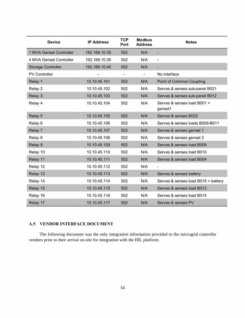
A.4 IP Address Mapping 53 A.5 Vendor Interface Document 54
References 85
ix
LIST OF ILLUSTRATIONS
Figure Page No.
1.1 Microgrid testbed types. 2
1.2 Tradeoffs between microgrid testbeds. 4
2.1 Sample interconnection setup of commercial controllers with the real-time simulator. 7
2.2 Timescales within the real-time controller hardware-in-the-loop system. 8
3.1 Test feeder one-line diagram. 11
3.2 Hardware setup of the controllers with the Opal-RT real time simulator. 12
3.3 Scheme of the dynamic load. 15
3.4 Sample input data to dynamic loads. 16
3.5 Relay modeling base-scheme. 17
3.6 Scheme of functions: undervoltage relay (27), AC inverse-time overcurrent relay (50), instantaneous overcurrent relay (51), and overvoltage relay (59). 18
3.7 Simulink model of the relay. 19
3.8 Simulink model of the synchronism-check function. 19
3.9 Caterpillar generator sets (CAT 32 and CAT C175-20). 21
3.10 Interface of (1000 kVA and 4000 kVA) generators with Woodward controllers. 21
3.11 Simulink base model of the (1000 kVA and 4000 kVA) generators. 22
3.12 The boost rectifier average model as the basis for both grid-tied inverters. 22
3.13 Inverter subsystem block level details. 23
3.14 Inverter current controller. 24
LIST OF ILLUSTRATIONS (Continued)
Figure No. Page
x
3.15 Boost rectifier plant model. 25
3.16 Curves for the PV panels used in the model. 26
3.17 PV subsystem block level detail. 27
3.18 Battery connected to the grid-tied inverter. 28
3.19 Connectivity scheme for generator models with the Woodward controllers. 29
3.20 Communication traffic between the microgrid controller and the test platform. 36
3.21 Power flow through PCC, generators, and battery – Vendor 1. 40
3.22 Power flow through PCC, generators, and battery – Vendor 2. 41
4.1 Anonymized results of microgrid controller demonstration cases. 44
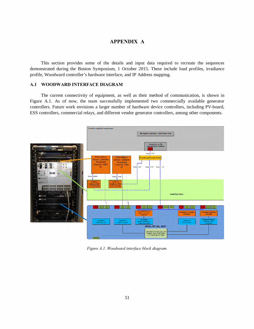
A.1 Woodward interface block diagram. 51
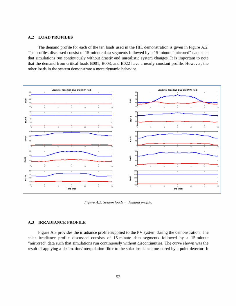
A.2 System loads − demand profile. 52
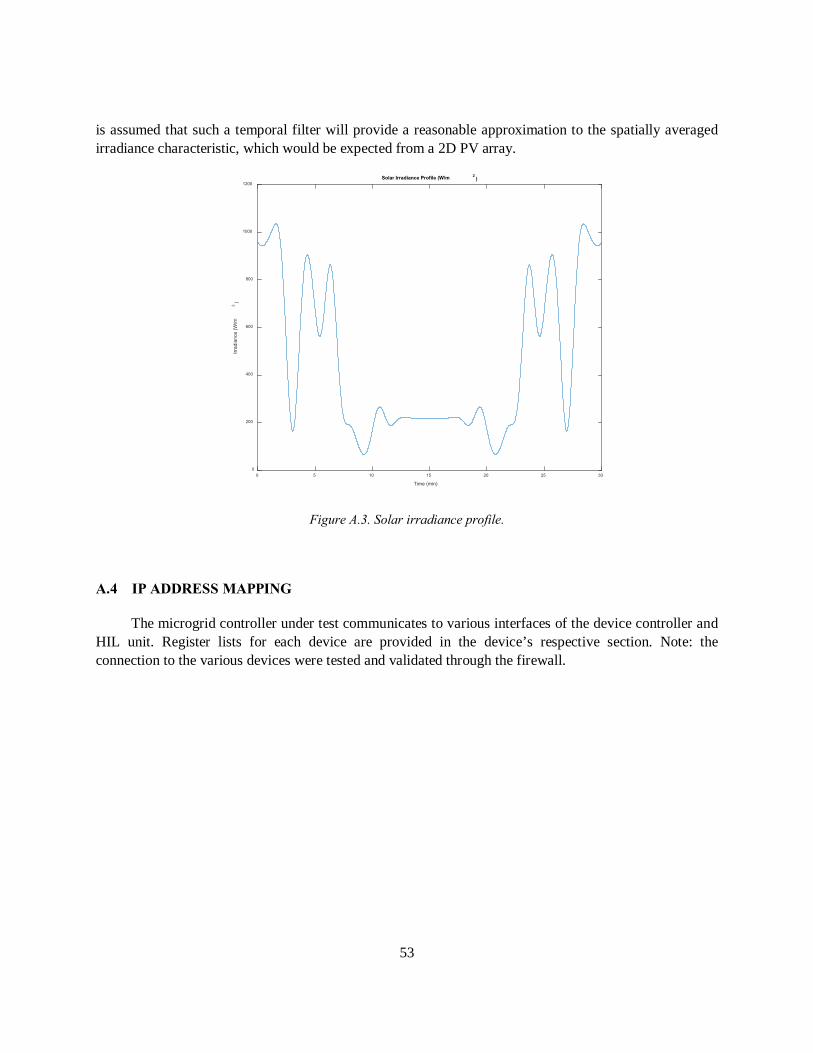
A.3 Solar irradiance profile. 53
xi
LIST OF TABLES
Table Page No.
1 Cable Impedances 14
2 PV Component Specifications 25
3 ESS Component Specifications 28
4 Woodward Digital Inputs and Outputs 30
5 Subset of Registers for Woodward easYgen 3500 (protocol 5010 [4], pp. 697−739) 32
6 Woodward easYgen 3500 Parameter ID 33
7 Load Categories 38
This page intentionally left blank.
1
1. BACKGROUND
Microgrids are systems of systems. The components that comprise microgrids – distributed energy resources (DERs), protection equipment, and distribution equipment – are complex systems in and of themselves. When combined to form a larger system, with nearly infinite possible combinations, these microgrids can exhibit unpredictable emergent behavior.
As a result, extensive and project-specific integration and interoperability testing are essential to ensure safe and reliable operation under the wide range of possible operating conditions. Microgrid controllers act as the nerve center of microgrid systems, tying together and coordinating the DER and other components. Microgrid controllers and the downstream device controllers they integrate are the crux of the microgrid deployment challenge.
Numerous issues, however, have been identified by industry as an impediment to efficient microgrid deployment.
• High non-recurring engineering (NRE) cost: Each project has a high NRE due to the project-specific integration and interoperability testing required.
• “Vaporware”: As new companies enter the market for microgrid controls, and established companies modify their existing products to address this new business opportunity, some have been accused of advertising functional capabilities that are not yet ready. When the time comes for deployment, it becomes apparent that these functions are under development and testing for the first time on that project.
• Risk of damage to expensive equipment: As cyber-physical industrial control systems, microgrid controllers and downstream controllers can malfunction and cause real physical damage to multi-megawatt pieces of equipment, with the associated cost, schedule, and safety concerns.
• Uncharacterized controls behavior: Because their controls behavior relies on proprietary software, the interconnection behavior of a microgrid – or even standalone DERs – is largely unknowable to utility power distribution engineers using existing industry engineer tools. The steady-state and transient analysis tools used by distribution system engineers cannot assess the dynamic control behavior of these new assets and systems.
• No standards verification: Industry-wide standards for microgrid controllers are nascent: IEEE is developing the P2030.7 Standard for the Specification of Microgrid Controllers, as well as P2030.8 Standard for the Testing of Microgrid Controllers; Duke Energy and its partners are developing the OpenFMB framework; and distribution utilities are just beginning to consider
2
their own specific regulations. Currently, no methods exist for cost-effectively testing microgrid designs against these standards or the requirements defined by project developers or end users.
The authors have concluded that a technology platform that facilitates the design, evaluation, commissioning testing, and standards compliance validation testing of microgrids could accelerate deployment of microgrids. The industry needs software development and integration work completed well in advance of construction of the microgrid. Projects would see a higher approval rate if the utility engineers and project developers perceived lower technical, safety, and financial risk. Due to the integration and testing challenges introduced by microgrid systems, this platform should focus on microgrid controllers and the assets they integrate.
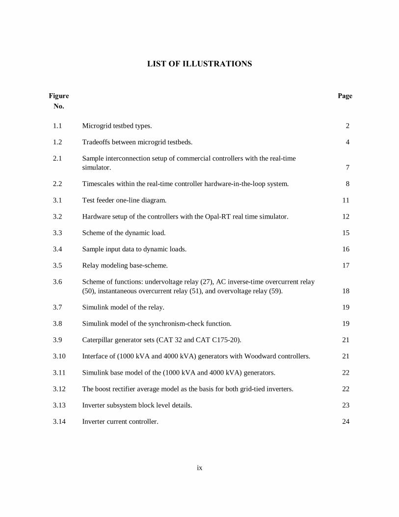
We segment microgrid testbeds – and advanced distribution testing – into five categories, shown in Figure 1.1.
Full System
Inv G
C C
Inv
Power Testbed
G
C C
Power HIL
Inv
C
G
C
Controller HIL
C
GInv
C
Simulation
GInv
CC
µC µC µC
DMS DMS
LegendG generatorInv battery or solar inverterC device controllerµC microgrid controllerDMS distribution management system controller
power gridhigh-bandwidth AC-AC convertersimulation or emulation boundary
hardwarevirtual (simulated or emulated)
Figure 1.1. Microgrid testbed types.
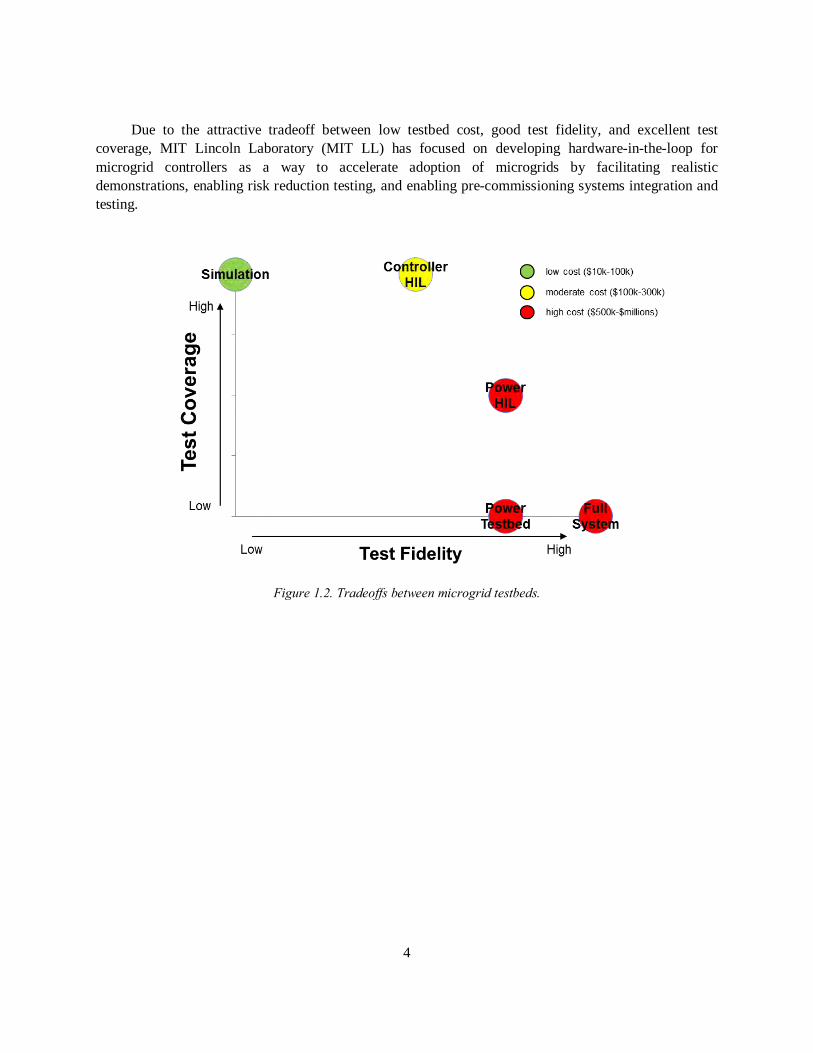
These categories of testbeds can be ranked based on the following categories, as summarized in Figure 1.2:
3
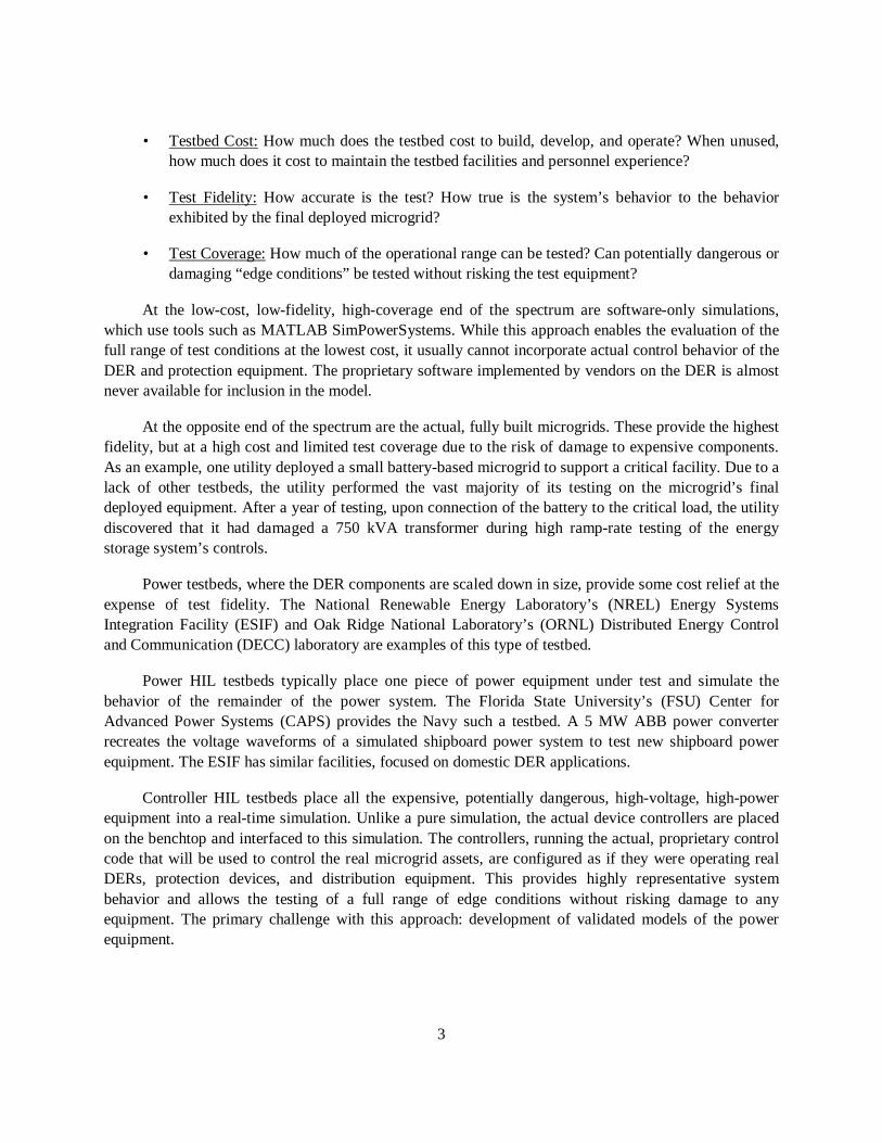
• Testbed Cost: How much does the testbed cost to build, develop, and operate? When unused, how much does it cost to maintain the testbed facilities and personnel experience?
• Test Fidelity: How accurate is the test? How true is the system’s behavior to the behavior exhibited by the final deployed microgrid?
• Test Coverage: How much of the operational range can be tested? Can potentially dangerous or damaging “edge conditions” be tested without risking the test equipment?
At the low-cost, low-fidelity, high-coverage end of the spectrum are software-only simulations, which use tools such as MATLAB SimPowerSystems. While this approach enables the evaluation of the full range of test conditions at the lowest cost, it usually cannot incorporate actual control behavior of the DER and protection equipment. The proprietary software implemented by vendors on the DER is almost never available for inclusion in the model.
At the opposite end of the spectrum are the actual, fully built microgrids. These provide the highest fidelity, but at a high cost and limited test coverage due to the risk of damage to expensive components. As an example, one utility deployed a small battery-based microgrid to support a critical facility. Due to a lack of other testbeds, the utility performed the vast majority of its testing on the microgrid’s final deployed equipment. After a year of testing, upon connection of the battery to the critical load, the utility discovered that it had damaged a 750 kVA transformer during high ramp-rate testing of the energy storage system’s controls.
Power testbeds, where the DER components are scaled down in size, provide some cost relief at the expense of test fidelity. The National Renewable Energy Laboratory’s (NREL) Energy Systems Integration Facility (ESIF) and Oak Ridge National Laboratory’s (ORNL) Distributed Energy Control and Communication (DECC) laboratory are examples of this type of testbed.
Power HIL testbeds typically place one piece of power equipment under test and simulate the behavior of the remainder of the power system. The Florida State University’s (FSU) Center for Advanced Power Systems (CAPS) provides the Navy such a testbed. A 5 MW ABB power converter recreates the voltage waveforms of a simulated shipboard power system to test new shipboard power equipment. The ESIF has similar facilities, focused on domestic DER applications.
Controller HIL testbeds place all the expensive, potentially dangerous, high-voltage, high-power equipment into a real-time simulation. Unlike a pure simulation, the actual device controllers are placed on the benchtop and interfaced to this simulation. The controllers, running the actual, proprietary control code that will be used to control the real microgrid assets, are configured as if they were operating real DERs, protection devices, and distribution equipment. This provides highly representative system behavior and allows the testing of a full range of edge conditions without risking damage to any equipment. The primary challenge with this approach: development of validated models of the power equipment.
4
Due to the attractive tradeoff between low testbed cost, good test fidelity, and excellent test coverage, MIT Lincoln Laboratory (MIT LL) has focused on developing hardware-in-the-loop for microgrid controllers as a way to accelerate adoption of microgrids by facilitating realistic demonstrations, enabling risk reduction testing, and enabling pre-commissioning systems integration and testing.
Figure 1.2. Tradeoffs between microgrid testbeds.
5
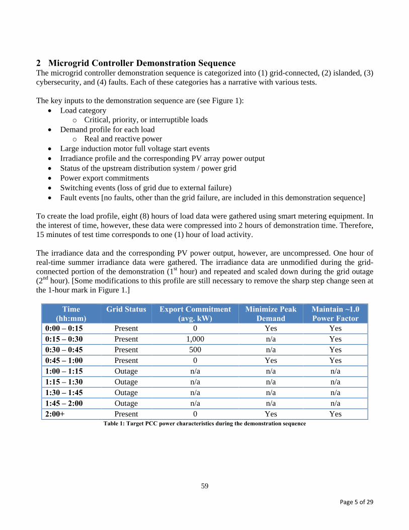
2. APPROACH
The vision for this work is to create a standardized demonstration and evaluation platform for any available commercial microgrid or device controller in the market using any distribution system topology. The outcome of this work will reduce microgrid development cost, validate marketing claims, and reduce risk of equipment damage, as well as reduce deployment time.
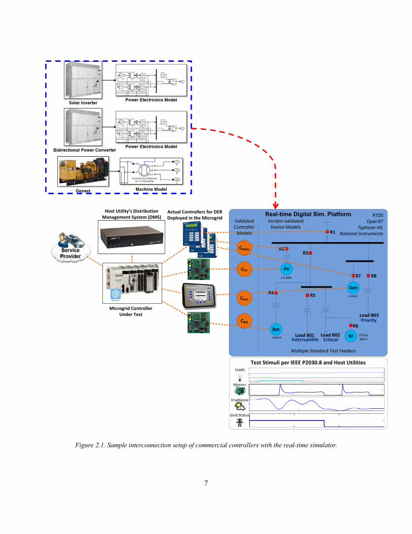
Figure 2.1 shows a diagram of the elements of the real-time microgrid controls demonstration platform. The stepwise approach for building this platform is as follows:
1. Microgrid feeder: Model the target microgrid distribution feeder and segment it into the processing cores of a real-time digital simulator. Multiple vendors sell real-time simulators, including OPAL-RT, Typhoon HIL, RTDS, and National Instruments. For this effort, MIT LL selected an OPAL-RT 5607, partly because it could accept models from MATLAB SimPowerSystems. The feeder was based on an anonymized feeder to which MIT LL had access to the detailed specifications of the transformers, conductors, protection devices, and loads.
2. Load and irradiance profiles: Assign a priority of Critical, Priority, or Interruptible to each load. Collect real load measurements on the test feeder at 1 second intervals. Collect a solar irradiance profile to simulate representative variation in solar energy production.
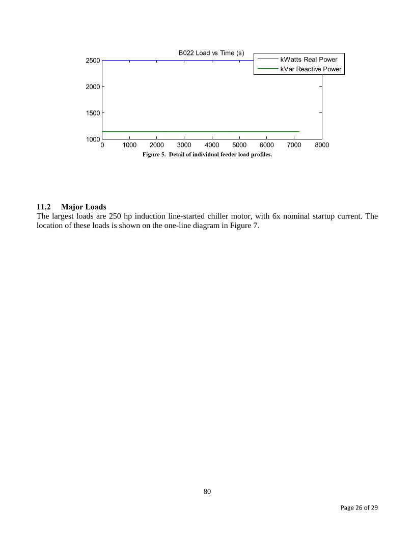
3. DER devices: Develop models of the physical DER devices, including gensets, a battery-based energy storage system with a bidirectional power converter, a solar photovoltaic (PV) system with inverter, and eighteen breakers. (Future work will require either validation of these models or replacement with vendor-provided models.)
4. Physical device controllers: Integrate commercial controllers with the simulated microgrid power devices. For both of the gensets in the simulation, integrate off-the-shelf Woodward easYgen 3000 controllers. Using the signal conditioning interface illustrated in Figure 3.19, the simulation of the physical genset and its subcomponents, and calibration, configure these controllers as if they were operating actual 1 MVA and 4 MVA, 13.8 kV gensets.
5. Software device controllers: Ideally, all of the controllable devices within the test would be operated by actual commercially available controllers. For those microgrid devices that are not operated by a commercial controller, develop custom control software. (For this project, this was done for the energy storage, solar PV, and breakers.) Implement several relay protection functions to actuate the breakers. Implement various control schemes – real/reactive power control, frequency and voltage control, maximum power point tracking within the PV inverter –on the DER controllers to enable the microgrid controllers flexibility in how they operated the system.
6
6. Manual testing: Once the elements listed above are successfully integrated, engineers can operate the microgrid by manually issuing dispatch commands and changing operating set-points within the system. Using a software interface, test the Modbus TCP communications with each device.
7. Additional test stimuli: Simulate grid outages, inrush currents from motor starts, and faults in various locations of the system in real time to increase the realism of the simulation. (For this initial demonstration, none of these additional stimuli were introduced. Intentional microgrid islanding – not unintentional islanding – was implemented by the microgrid controllers.)
8. Microgrid controllers: Lastly, integrate commercial microgrid controllers in collaboration with these companies’ engineers. (Schneider and Eaton controllers were integrated for this demonstration.) Protocol converters may be needed to translate the communications from the microgrid controller to Modbus TCP, and to map the microgrid controller’s register list to the communication registers used by the software and hardware device controllers.
9. Test and collect data: Execute test sequences under a variety of load, irradiance, fault, and grid stimuli. Collect communications data, estimated fuel consumption, power generation, data on voltage and frequency quality, and load service information.
10. Post-process data for performance metrics: Use the data to quantify performance of the microgrid controllers, compare performance between vendors, and identify potential areas for additional testing and development.
7
Test Stimuli per IEEE P2030.8 and Host Utilities
Real-time Digital Sim. Platform
Load .01 Load .02
Load .03
3.5 MW
4 MVA
4 MVA
R1
R8R7
R5Den
a 250 hp460 V
R6
PV
.at
Interruptible Critical
Priority
CDen
CRelay
Multiple Standard Test Feeders
C.at
Loads
Motors
Irradiance
Grid Status
R4
R2R3
Actual Controllers for DER Deployed in the aicrogrid
aicrogrid ControllerUnder Test
Host Utility’s Distribution aanagement System (DaS) RTDS
Opal-RTTyphoon HIL
National Instruments
Vendor-validated Device Models
Validated Controller
Models
CPV
Figure 2.1. Sample interconnection setup of commercial controllers with the real-time simulator.
8
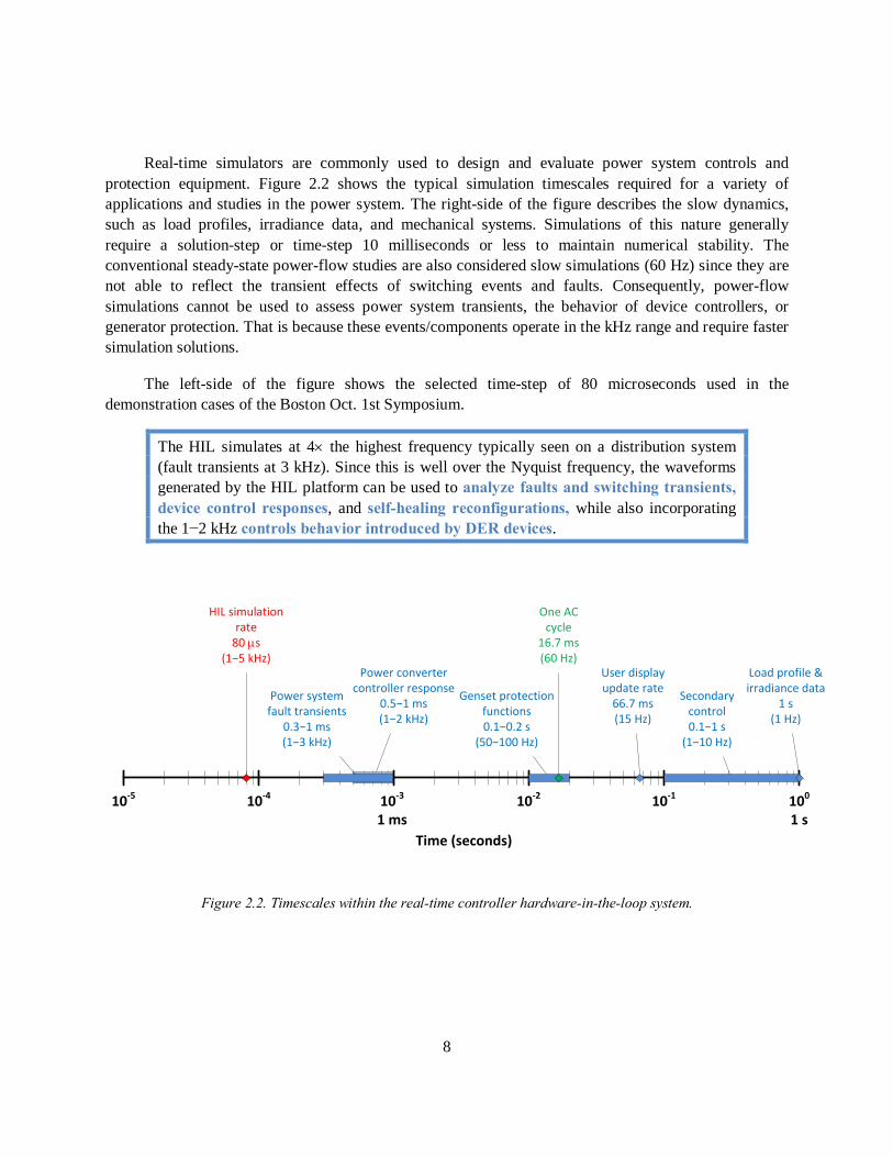
Real-time simulators are commonly used to design and evaluate power system controls and
protection equipment. Figure 2.2 shows the typical simulation timescales required for a variety of applications and studies in the power system. The right-side of the figure describes the slow dynamics, such as load profiles, irradiance data, and mechanical systems. Simulations of this nature generally require a solution-step or time-step 10 milliseconds or less to maintain numerical stability. The conventional steady-state power-flow studies are also considered slow simulations (60 Hz) since they are not able to reflect the transient effects of switching events and faults. Consequently, power-flow simulations cannot be used to assess power system transients, the behavior of device controllers, or generator protection. That is because these events/components operate in the kHz range and require faster simulation solutions.
The left-side of the figure shows the selected time-step of 80 microseconds used in the demonstration cases of the Boston Oct. 1st Symposium.
The HIL simulates at 4× the highest frequency typically seen on a distribution system (fault transients at 3 kHz). Since this is well over the Nyquist frequency, the waveforms generated by the HIL platform can be used to analyze faults and switching transients, device control responses, and self-healing reconfigurations, while also incorporating the 1−2 kHz controls behavior introduced by DER devices.
10-5 10-4 10-3
1 ms10-2 10-1 100
1 sTime (seconds)
HIL simulation rate
80 µs(1−5 kHz)
One AC cycle
16.7 ms(60 Hz)
User display update rate
66.7 ms(15 Hz)
Load profile & irradiance data
1 s(1 Hz)
Power converter controller response
0.5−1 ms(1−2 kHz)
Secondary control0.1−1 s
(1−10 Hz)
Power system fault transients
0.3−1 ms(1−3 kHz)
Genset protection functions0.1−0.2 s
(50−100 Hz)
Figure 2.2. Timescales within the real-time controller hardware-in-the-loop system.
9
3. SYSTEM UNDER STUDY
3.1 DISTRIBUTION SYSTEM MODELING
3.1.1 Network Architecture
Radial distribution systems are widely implemented due to their simplicity and relatively low cost. The feeders leave a substation and distribute electrical power in the designated zone without connections to other points of supply. This configuration is popular in rural areas with long feeders supplying remote loads. To increase reliability, damaged parts of the feeders may be isolated and alternative power sources (i.e. nearby substations or local generation) can be connected by means of manual or automatic tie switches.
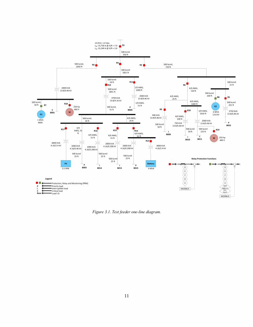
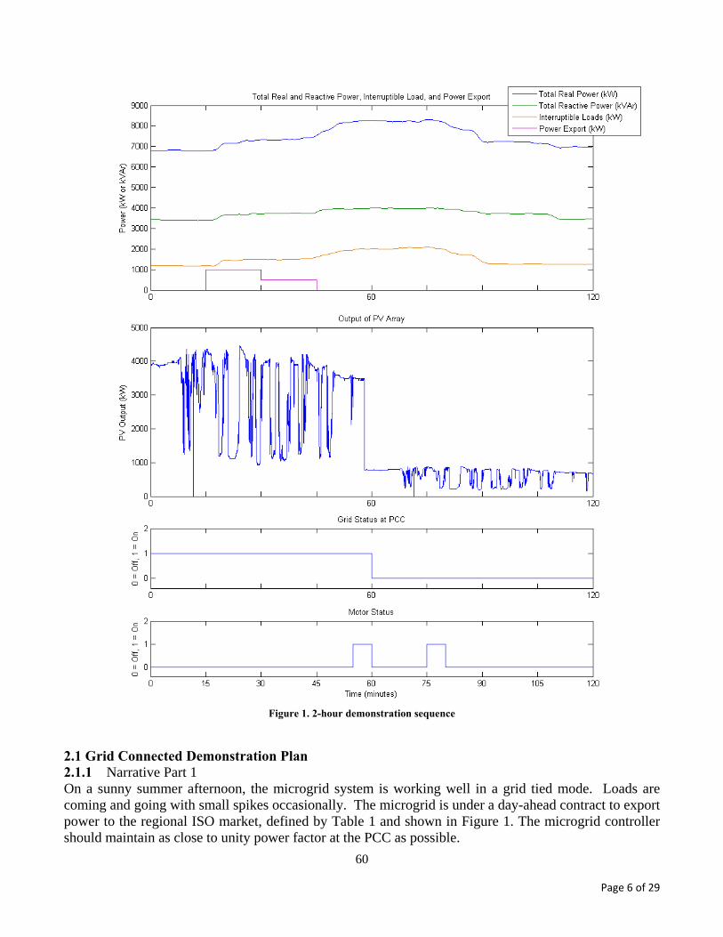
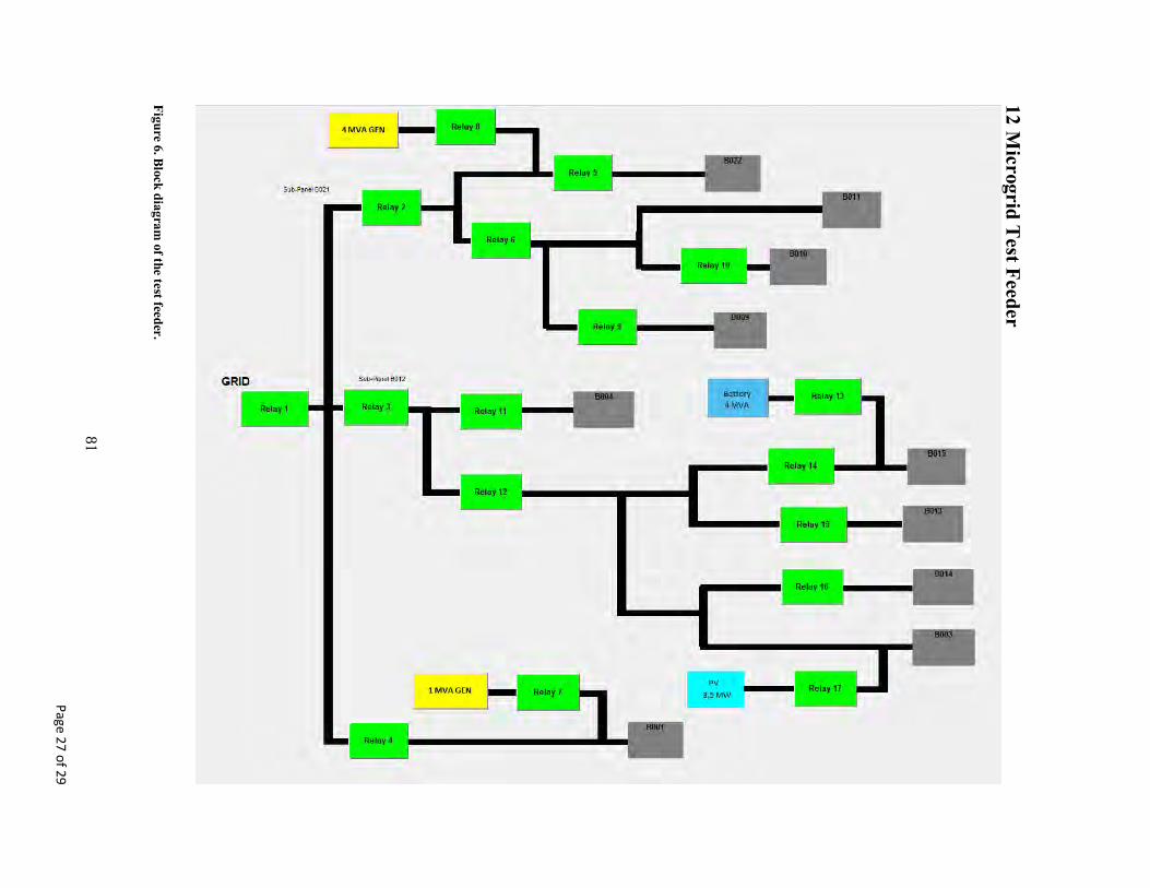
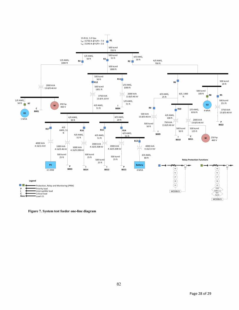
The test feeder used for the study consists of one (out-of-three) radial feeder supplying a real-life industrial park; see Figure 3.1. The overall electrical demand of the feeder ranges from 4.2 MW to 12 MW for minimum and maximum load, respectively. The system is rated for a medium voltage of 13.8 kV and low voltages of 4.16 kV, 2.4 kV, 460 V, and 208 V. There are 10 loads continuously supplied by the feeder (2 critical, 4 priority, and 4 interruptible). Critical loads are categorized by the high requirements of continuous electrical service, power quality, and reliability (i.e., hospitals, sensitive equipment labs, etc.). Priority loads are buildings that ideally are always served, but in case of contingencies, or islanding with lack of generation, may be disconnected. Interruptible loads are buildings not necessarily required to be served during contingencies or islanded conditions. Furthermore, there are two large induction motors of 250 horsepower, one of the largest sizes recommended by the National Electric Code (NEC) for full voltage start-up [2]. Even though these motors are not part of the actual site, the units were added to evaluate the microgrid controller's ability to perform islanded-load-balancing while having a large motors start-up.
Each of the system loads is modeled as a time-varying dynamic load based on electrical demand profiles extracted from smart metering equipment. These profiles are provided in Section A.2. There are two simulated Caterpillar diesel generators in the system corresponding to a 1000 kVA (CAT 32) and a 4000 kVA (CAT C175-20), operated at nominal voltages of 480 V and 13.8 kV, respectively [3]. Both generators are controlled and protected using the commercially available Woodward EasYgen 3500 generator controllers; see Figure 3.2 [4]. During simulations, the Woodward controllers are entirely controlled by the microgrid controllers without operator intervention unless the alarms deem necessary. Further discussion on the generator models is given in Section 3.1.9. There are 13 distribution transformers serving the area. Two of these transformers interconnect a simulated 3500 kW PV system with maximum power point tracking (MPPT), and a 4000 kVA energy storage system (ESS). The PV system is supplied with a varying irradiance profile that begins with a sunny day followed by a storm-type cloud. Note that any irradiance profile may be applied to the PV system. The ESS is fully controlled by the microgrid controller enabling the evaluation of power factor correction, peak shaving/smoothing, and
10
possibly power export. The total system demand, and the available generation and storage, were sized to evaluate the microgrid controller’s ability to perform smart load shedding prior and during islanded conditions.
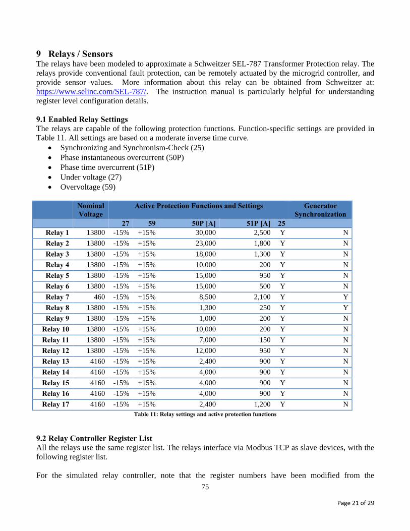
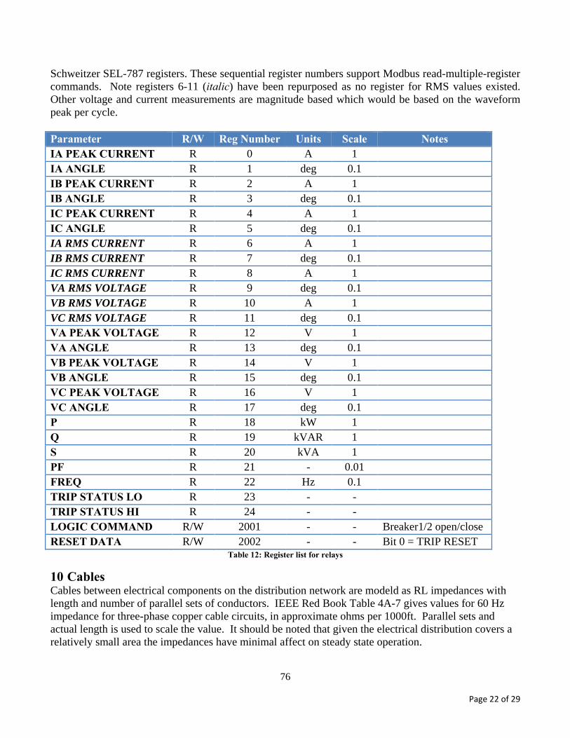
The conventional system fault protection is provided by simulated relays modeled to approximate a Schweitzer SEL-787 transformer protection relay [5]. These units can be remotely actuated by the microgrid controller and provide sensor values. All settings are based on a moderate inverse time curve. The simulated relay functions are the following: synchronizing or synchronism-check (ANSI Std. Dev. No. 25), phase instantaneous overcurrent (ANSI Std. Dev. No. 50P), AC inverse time overcurrent (ANSI Std. Dev. No. 51P), undervoltage relay (ANSI Std. Dev. No. 27), and overvoltage relay (ANSI Std. Dev. No. 59). Addition of other relay functions may be a topic for future development. Section 3.1.8 provides a detailed description of the relay model. The following sections will provide a more detailed discussion of each of the components used in the system, their operation modes, and interfaces.
11
C.001
P.003
I.014
I.013
P.015
I.009
I.010
C.011
P.022
P.004
Protection, Relay and Monitoring (PRM)
13.8 kV, 1.0 VpuI3ɸ: 15,730 A @ X/R = 7.9I1ɸ: 15,240 A @ X/R = 2.6
Figure 3.2. Hardware setup of the controllers with the Opal-RT real time simulator.
3.1.2 Modeling Approach
Since distribution systems consist of a large number of similar elements, the following modeling approach was adopted. The GUI of MATLAB-Simulink is used to derive detailed prototype models for each group of electrical components (i.e., one base model for all network transformers, one base model for all breakers, and so forth). These models are parametrized in order to adapt to different voltages, kVA ratings, operation settings, and impedances. Applying this technique, the following prototype models were derived:
• Cables
• Breakers
• Network transformers
• Time-varying loads
• Generators
• PV system
13
• Energy storage system (ESS)
• Relays simulating functions of the commercial SEL-787
In addition, some built-in models in the MATLAB-Simulink libraries were adopted, such as three-phase series RL branches, ideal switches, and measurement probes, among others. The created prototype models were placed into the system replicating the one-line diagram (see Figure 3.1). Then, the corresponding parameters of the prototype models were updated to reproduce the real-life system architecture. The resulting distribution system is then loaded into the real-time simulator, which is hardware-interfaced with two commercial Woodward EasYgen 3500 controllers and the commercial microgrid controller under evaluation. In the following subsections, the prototype models are described in more detail to provide more information on model complexity.
3.1.3 Utility Grid Model
The upstream utility electrical system is currently represented using the Thevenin equivalent provided in the electrical records of the site. These include nominal voltage, single-phase and three-phase short circuit powers at the point of common coupling (PCC), and the corresponding X/R ratios for single-phase and three-phase short circuits (see Figure 3.1). It may be desirable and a possibility of future work to model the upstream power system to evaluate the influence of microgrid controller operations to neighboring feeders supplied via the same substation as the microgrid.
3.1.4 Cable Models
Feeder conductors and secondary mains are modeled using positive sequences of three-phase series RL branches. Future work will involve cable modeling using PI sections with mutual inductances and capacitances between the phases. This will enable the accurate simulation of unbalanced system conditions such as the influence of single-phase short circuits on unfaulted phases. Parameters of each cable section were calculated using impedances obtained from IEEE 141-1993, Table 4A-7b, [1] and the length of the cables extracted from the actual site one-line diagram. Table 1 shows the most typical cables in the system.
14
TABLE 1
Cable Impedances
AWG/kcmil Resistance
[Ohms/1000 ft] Reactance
[Ohms/1000 ft]
1/0 0.128 0.0414
2/0 0.102 0.0407
4/0 0.064 0.0381
350 0.0378 0.0373
500 0.0294 0.0349
3.1.5 Breaker Model
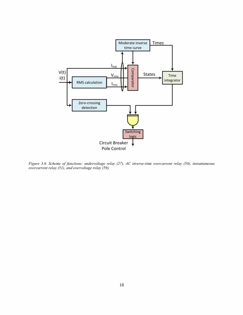
The circuit breakers are represented as controlled three-phase switches with measurement probes to monitor the system. Their control logic is provided by the relays as shown schematically in Figure 3.6. As can be seen in this figure, measured values of the phase currents flowing through the breaker and terminal voltages are compared with the selected overcurrent settings (instantaneous overcurrent or ac-time overcurrent) and under/over-voltage settings. Once tripping conditions are satisfied, the logic waits for current zero-crossing to issue the trip command.
After the trip command is issued, the switches wait a prespecified period of time to open, which models the mechanical delay of the actual device. Each breaker in the distribution system has its own tripping current and delay settings. The under/over-voltage settings are set to ±15% of nominal voltage. In addition, the developed switching logic of the model allows for commanded (manual) opening and reclosing of every breaker in the system. Other applicable logic to the circuit breaker includes the synchronism check; these functions will be described in detail in Section 3.1.8.
3.1.6 Network Transformer Models
The network transformer is implemented using three single-phase transformers connected in D/Y grounded configuration with a negative 30 degrees angular displacement, and operated with fixed-turn ratios. The impedances and X/R ratios were obtained from the actual site one-line diagram. Due to the short timeline of the effort, the units were modeled as linear transformers with magnetizing branches represented by constant per unit values of resistance and inductance. Although this assumption was not influential in the presented demos during the symposium, future work involving transient overvoltages, unbalanced short circuits, and self-healing switching may require the transformers to be modeled considering nonlinear magnetizing branches.
15
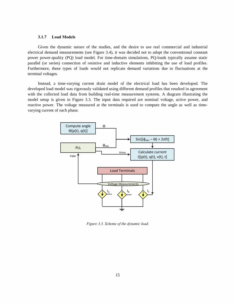
3.1.7 Load Models
Given the dynamic nature of the studies, and the desire to use real commercial and industrial electrical demand measurements (see Figure 3.4), it was decided not to adopt the conventional constant power power-quality (PQ) load model. For time-domain simulations, PQ-loads typically assume static parallel (or series) connection of resistive and inductive elements inhibiting the use of load profiles. Furthermore, these types of loads would not replicate demand variations due to fluctuations at the terminal voltages.
Instead, a time-varying current drain model of the electrical load has been developed. The developed load model was rigorously validated using different demand profiles that resulted in agreement with the collected load data from building real-time measurement systems. A diagram illustrating the model setup is given in Figure 3.3. The input data required are nominal voltage, active power, and reactive power. The voltage measured at the terminals is used to compute the angle as well as time-varying current of each phase.
Compute angle
Ө[p(t), q(t)]
PLL
Sin[(ɸabc – Ө) + 2πft]
Calculate currentI[(p(t), q(t), v(t), t]
Ө
ɸabc
Ia Ib Ic
Voltage Measurements
Load Terminals
VabcVrms
Figure 3.3. Scheme of the dynamic load.
16
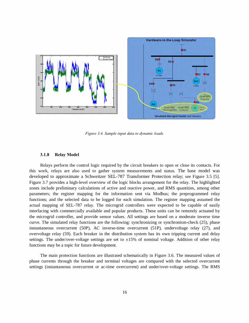
Figure 3.4. Sample input data to dynamic loads.
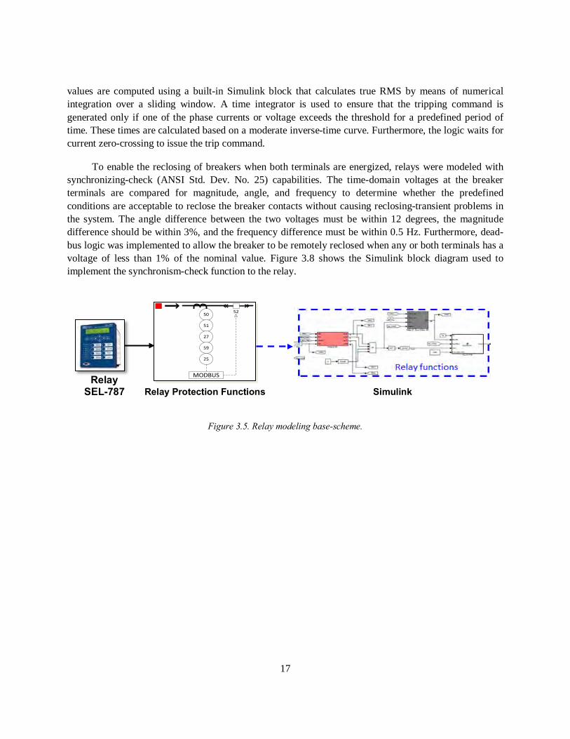
3.1.8 Relay Model
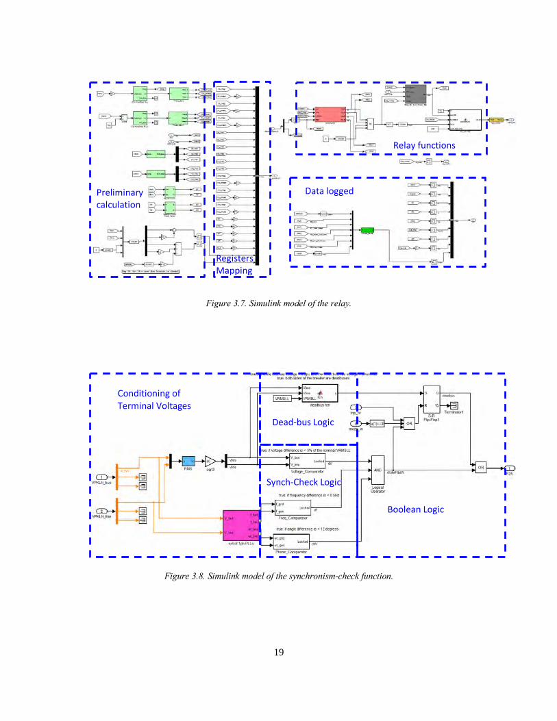
Relays perform the control logic required by the circuit breakers to open or close its contacts. For this work, relays are also used to gather system measurements and status. The base model was developed to approximate a Schweitzer SEL-787 Transformer Protection relay; see Figure 3.5 [5]. Figure 3.7 provides a high-level overview of the logic blocks arrangement for the relay. The highlighted zones include preliminary calculations of active and reactive power, and RMS quantities, among other parameters; the register mapping for the information sent via Modbus; the preprogrammed relay functions; and the selected data to be logged for each simulation. The register mapping assumed the actual mapping of SEL-787 relay. The microgrid controllers were expected to be capable of easily interfacing with commercially available and popular products. These units can be remotely actuated by the microgrid controller, and provide sensor values. All settings are based on a moderate inverse time curve. The simulated relay functions are the following: synchronizing or synchronism-check (25), phase instantaneous overcurrent (50P), AC inverse-time overcurrent (51P), undervoltage relay (27), and overvoltage relay (59). Each breaker in the distribution system has its own tripping current and delay settings. The under/over-voltage settings are set to ±15% of nominal voltage. Addition of other relay functions may be a topic for future development.
The main protection functions are illustrated schematically in Figure 3.6. The measured values of phase currents through the breaker and terminal voltages are compared with the selected overcurrent settings (instantaneous overcurrent or ac-time overcurrent) and under/over-voltage settings. The RMS
17
values are computed using a built-in Simulink block that calculates true RMS by means of numerical integration over a sliding window. A time integrator is used to ensure that the tripping command is generated only if one of the phase currents or voltage exceeds the threshold for a predefined period of time. These times are calculated based on a moderate inverse-time curve. Furthermore, the logic waits for current zero-crossing to issue the trip command.
To enable the reclosing of breakers when both terminals are energized, relays were modeled with synchronizing-check (ANSI Std. Dev. No. 25) capabilities. The time-domain voltages at the breaker terminals are compared for magnitude, angle, and frequency to determine whether the predefined conditions are acceptable to reclose the breaker contacts without causing reclosing-transient problems in the system. The angle difference between the two voltages must be within 12 degrees, the magnitude difference should be within 3%, and the frequency difference must be within 0.5 Hz. Furthermore, dead-bus logic was implemented to allow the breaker to be remotely reclosed when any or both terminals has a voltage of less than 1% of the nominal value. Figure 3.8 shows the Simulink block diagram used to implement the synchronism-check function to the relay.
Figure 3.5. Relay modeling base-scheme.
50
51
27
59
25
MODBUS
52
Relay Protection Functions Relay
SEL-787 Simulink
18
RMS calculation
Time integrator
Switching logic
Vrms
Zero-crossing detection
Comparator
Moderate inverse time curve
Irms
Iinst
V(t)i(t)
Times
States
Circuit Breaker Pole Control
Figure 3.6. Scheme of functions: undervoltage relay (27), AC inverse-time overcurrent relay (50), instantaneous overcurrent relay (51), and overvoltage relay (59).
19
Figure 3.7. Simulink model of the relay.
Figure 3.8. Simulink model of the synchronism-check function.
Relay functions
Data logged
Registers Mapping
Preliminary calculation
Conditioning of Terminal Voltages
Synch-Check Logic
Dead-bus Logic
Boolean Logic
20
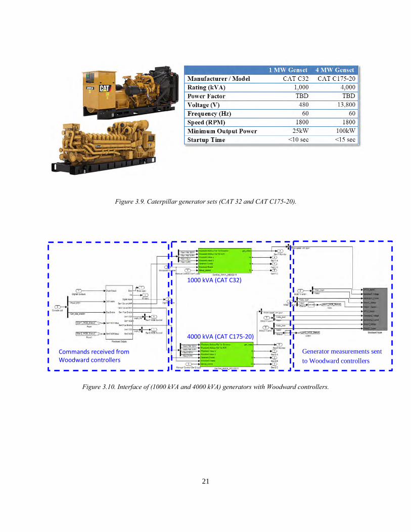
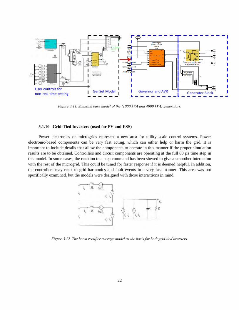
3.1.9 Generator Model
The two simulated Caterpillar diesel generators in the system correspond to a 1000 kVA (CAT 32) and a 4000 kVA (CAT C175-20), operated at nominal voltages of 480 V and 13.8 kV, respectively (see Figure 3.9) [3]. Figure 3.10 shows the interfaces of the Woodward easYgen controllers with the simulated 1000 kVA generator and 4000 kVA generators. The Woodward communicates to the vendor microgrid controller via a Modbus interface. However, all communications, such as generator commands and (voltage/frequency) set points, are sent from the Woodward controllers to the Opal-RT simulated system using digital I/O channels. Further discussion on the Woodward and its topology is provided in Section 3.2.
The generators consist of the numerical representation of a diesel engine (prime mover) and alternator (synchronous motor); see Figure 3.11. The Automatic Voltage Regulator (AVR) controls the synchronous machine’s field voltage, and the governor regulates the diesel engine’s throttle to control frequency. The voltage and frequency set points of the governor and AVR are adjusted by the secondary-level generator controller (i.e., Woodward easYgen 3500). The adjustments of voltage and frequency set points allow for synchronization and control of real and reactive power output of the generator unit. Two independent low-latency control inner-loops, in the order of milliseconds, are used to regulate output voltage and output frequency. While these two loops are controlled separately, their effects are coupled. Say, when the AVR increases voltage it will cause the generator frequency to drop, thus the governor will have to increase power to maintain its frequency set point. Likewise, if the governor increases power, then the AVR will need to compensate to maintain voltage. The low-level generator model control loops, AVR and governor, are evolved and customized versions of the built-in MATLAB SimPowerSystems Hydro Quebec toolset.
These two low-level inner control loops are typically simple PID controllers from different manufacturers. High-level control schemes such as frequency droop, voltage droop, and synchronization, as well as other refinements to power quality, are implemented via the secondary-level controllers, in this case, the Woodward controllers. The generator manufacturer typically tunes these two control loops over a variety of operating conditions to ensure stability and a quick response to perturbations. Since these tuning parameters are unavailable to customers, a set of parameters was chosen that most closely reproduces the expected dynamic behavior of the CAT 32 and CAT C175-20 generators.
21
Figure 3.9. Caterpillar generator sets (CAT 32 and CAT C175-20).
Figure 3.10. Interface of (1000 kVA and 4000 kVA) generators with Woodward controllers.
Generator measurements sent to Woodward controllers
Commands received from Woodward controllers
4000 kVA (CAT C175-20)
1000 kVA (CAT C32)
22
Figure 3.11. Simulink base model of the (1000 kVA and 4000 kVA) generators.
3.1.10 Grid-Tied Inverters (used for PV and ESS)
Power electronics on microgrids represent a new area for utility scale control systems. Power electronic-based components can be very fast acting, which can either help or harm the grid. It is important to include details that allow the components to operate in this manner if the proper simulation results are to be obtained. Controllers and circuit components are operating at the full 80 µs time step in this model. In some cases, the reaction to a step command has been slowed to give a smoother interaction with the rest of the microgrid. This could be tuned for faster response if it is deemed helpful. In addition, the controllers may react to grid harmonics and fault events in a very fast manner. This area was not specifically examined, but the models were designed with those interactions in mind.
Figure 3.12. The boost rectifier average model as the basis for both grid-tied inverters.
GenSet Model User controls for non-real time testing Governor and AVR Generator Block
23
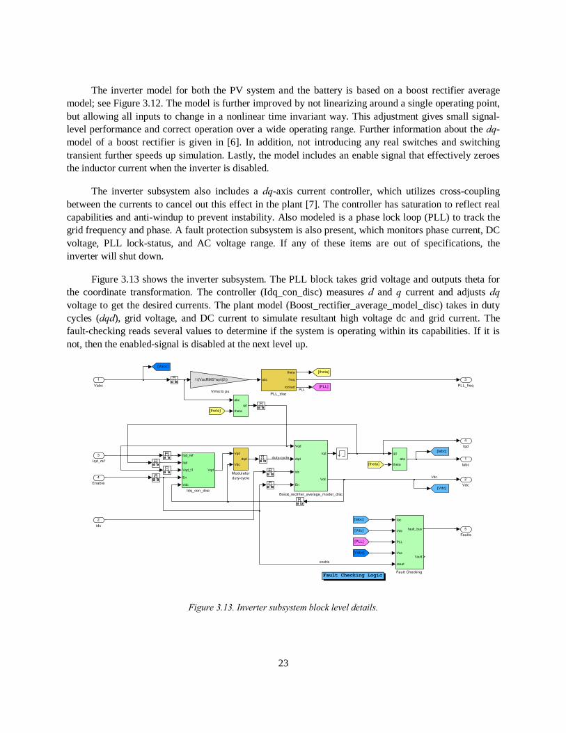
The inverter model for both the PV system and the battery is based on a boost rectifier average model; see Figure 3.12. The model is further improved by not linearizing around a single operating point, but allowing all inputs to change in a nonlinear time invariant way. This adjustment gives small signal-level performance and correct operation over a wide operating range. Further information about the dq-model of a boost rectifier is given in [6]. In addition, not introducing any real switches and switching transient further speeds up simulation. Lastly, the model includes an enable signal that effectively zeroes the inductor current when the inverter is disabled.
The inverter subsystem also includes a dq-axis current controller, which utilizes cross-coupling between the currents to cancel out this effect in the plant [7]. The controller has saturation to reflect real capabilities and anti-windup to prevent instability. Also modeled is a phase lock loop (PLL) to track the grid frequency and phase. A fault protection subsystem is also present, which monitors phase current, DC voltage, PLL lock-status, and AC voltage range. If any of these items are out of specifications, the inverter will shut down.
Figure 3.13 shows the inverter subsystem. The PLL block takes grid voltage and outputs theta for the coordinate transformation. The controller (Idq_con_disc) measures d and q current and adjusts dq voltage to get the desired currents. The plant model (Boost_rectifier_average_model_disc) takes in duty cycles (dqd), grid voltage, and DC current to simulate resultant high voltage dc and grid current. The fault-checking reads several values to determine if the system is operating within its capabilities. If it is not, then the enabled-signal is disabled at the next level up.
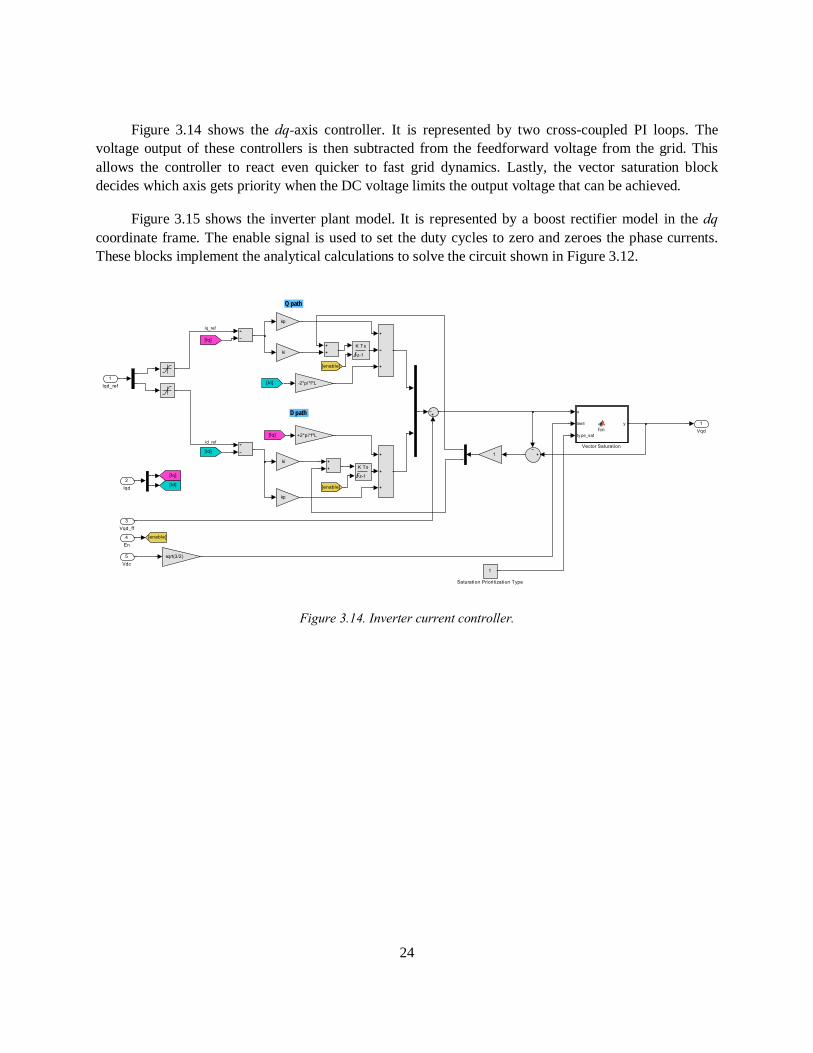
Figure 3.14 shows the dq-axis controller. It is represented by two cross-coupled PI loops. The voltage output of these controllers is then subtracted from the feedforward voltage from the grid. This allows the controller to react even quicker to fast grid dynamics. Lastly, the vector saturation block decides which axis gets priority when the DC voltage limits the output voltage that can be achieved.
Figure 3.15 shows the inverter plant model. It is represented by a boost rectifier model in the dq coordinate frame. The enable signal is used to set the duty cycles to zero and zeroes the phase currents. These blocks implement the analytical calculations to solve the circuit shown in Figure 3.12.
Figure 3.14. Inverter current controller.
Q path
D path1
Vqd
u
limit
ty pe_sat
yfcn
Vector Saturation
1
Saturation Prioritization Type
[Id]
[Iq]
[enable]
1
+2*pi*f*L
kp
sqrt(3/2)
ki
kp
-2*pi*f*L
ki
[Iq]
[Id]
[Id]
[Iq]
[enable]
[enable]
K Ts
z-1
K Ts
z-1
5Vdc
4En
3Vqd_ff
2Iqd
1Iqd_ref
Id_ref
Iq_ref
25
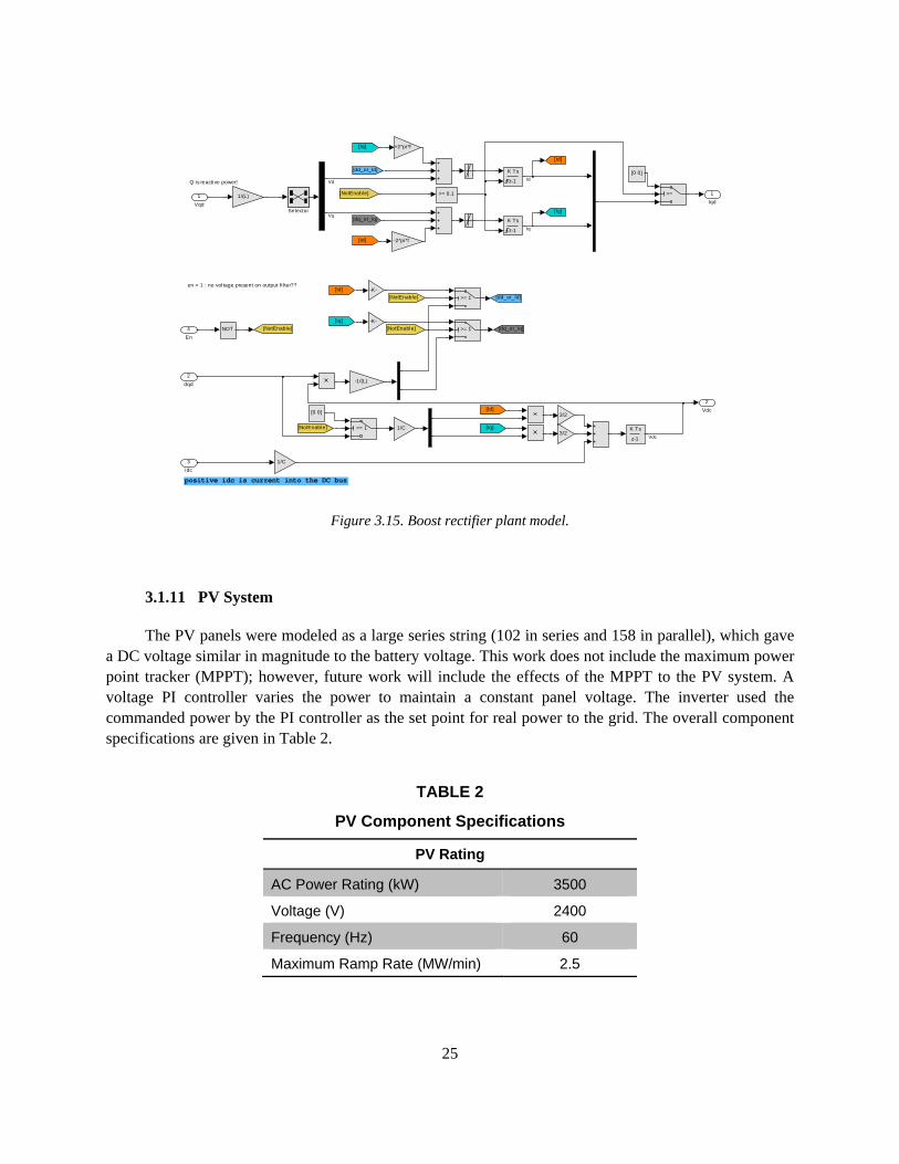
Figure 3.15. Boost rectifier plant model.
3.1.11 PV System
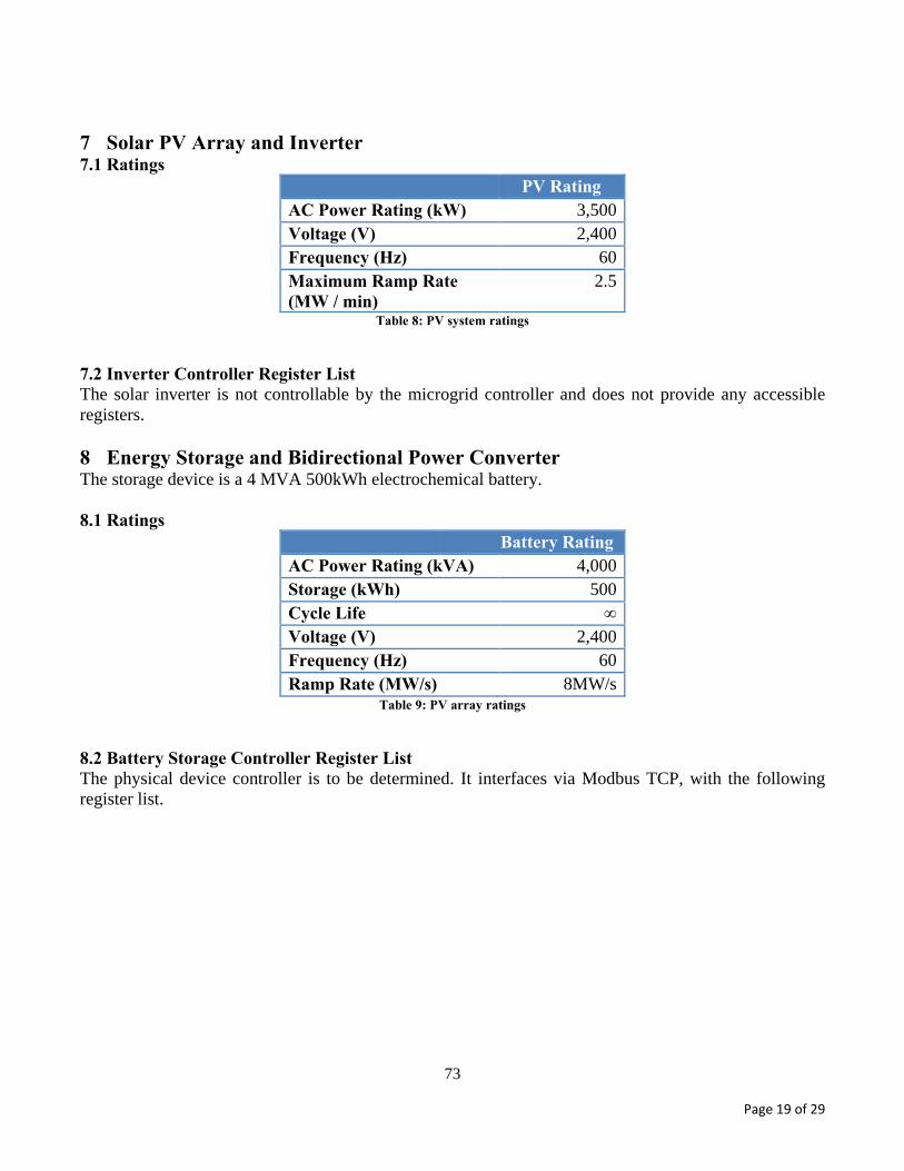
The PV panels were modeled as a large series string (102 in series and 158 in parallel), which gave a DC voltage similar in magnitude to the battery voltage. This work does not include the maximum power point tracker (MPPT); however, future work will include the effects of the MPPT to the PV system. A voltage PI controller varies the power to maintain a constant panel voltage. The inverter used the commanded power by the PI controller as the set point for real power to the grid. The overall component specifications are given in Table 2.
TABLE 2
PV Component Specifications
PV Rating
AC Power Rating (kW) 3500
Voltage (V) 2400
Frequency (Hz) 60
Maximum Ramp Rate (MW/min) 2.5
positive idc is current into the DC bus
Q is reactive power!
en = 1 : no voltage present on output fi l ter??
2Vdc
1Iqd
>= 1
>=
>= 1
>= 1
Selector
NOT
[Iq]
[Id]
[dd_or_Id]
[dq_or_Iq][NotEnable]
3/2
-K-
-K-
1/C
-1/(L)
-2*pi*f
+2*pi*f
1/C3/2
1/(L)
[Iq]
[dd_or_Id]
[dq_or_Iq]
[NotEnable]
[NotEnable]
[NotEnable]
[Iq]
[Id]
[Iq]
[Id]
[Id]
[NotEnable]
K Ts
z-1
K Ts
z-1
K Ts
z-1
[0 0]
[0 0]
>= 0.1
4En
3idc
2dqd
1Vqd
Vdc
Id
Iq
Vd
Vq
26
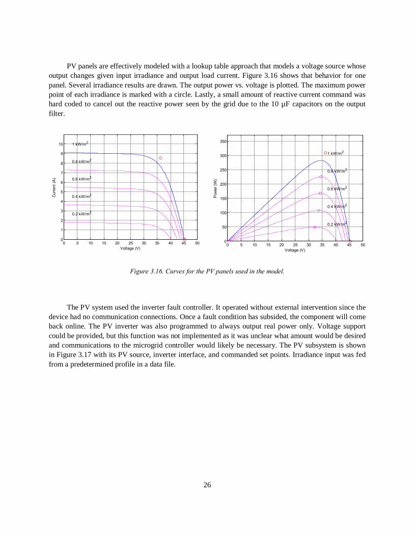
PV panels are effectively modeled with a lookup table approach that models a voltage source whose output changes given input irradiance and output load current. Figure 3.16 shows that behavior for one panel. Several irradiance results are drawn. The output power vs. voltage is plotted. The maximum power point of each irradiance is marked with a circle. Lastly, a small amount of reactive current command was hard coded to cancel out the reactive power seen by the grid due to the 10 µF capacitors on the output filter.
Figure 3.16. Curves for the PV panels used in the model.
The PV system used the inverter fault controller. It operated without external intervention since the device had no communication connections. Once a fault condition has subsided, the component will come back online. The PV inverter was also programmed to always output real power only. Voltage support could be provided, but this function was not implemented as it was unclear what amount would be desired and communications to the microgrid controller would likely be necessary. The PV subsystem is shown in Figure 3.17 with its PV source, inverter interface, and commanded set points. Irradiance input was fed from a predetermined profile in a data file.
0 5 10 15 20 25 30 35 40 45 500
1
2
3
4
5
6
7
8
9
10 1 kW/m2
Cur
rent
(A)
Voltage (V)
0.8 kW/m2
0.6 kW/m2
0.4 kW/m2
0.2 kW/m2
0 5 10 15 20 25 30 35 40 45 500
50
100
150
200
250
300
350
1 kW/m2
Pow
er (W
)
Voltage (V)
0.8 kW/m2
0.6 kW/m2
0.4 kW/m2
0.2 kW/m2
27
Figure 3.17. PV subsystem block level detail.
3.1.12 Energy Storage System (ESS)
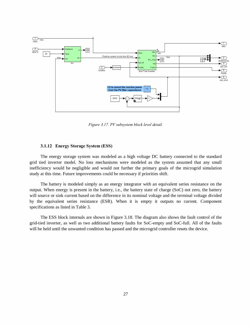
The energy storage system was modeled as a high voltage DC battery connected to the standard grid tied inverter model. No loss mechanisms were modeled as the system assumed that any small inefficiency would be negligible and would not further the primary goals of the microgrid simulation study at this time. Future improvements could be necessary if priorities shift.
The battery is modeled simply as an energy integrator with an equivalent series resistance on the output. When energy is present in the battery, i.e., the battery state of charge (SoC) not zero, the battery will source or sink current based on the difference in its nominal voltage and the terminal voltage divided by the equivalent series resistance (ESR). When it is empty it outputs no current. Component specifications as listed in Table 3.
The ESS block internals are shown in Figure 3.18. The diagram also shows the fault control of the grid-tied inverter, as well as two additional battery faults for SoC-empty and SoC-full. All of the faults will be held until the unwanted condition has passed and the microgrid controller resets the device.
-12 to cancel the reactive powerfrom the PV filter capacitance
Positive current is into the DC bus.
5Faults
4Iqd_cmd
3Iqd_act
2BatteryVars
1Iabc
PID(z)
Irradiance
Temp
Vpv
m
Ipv
PV
Vabc
idc
Iqd_ref
Enable
Iabc
Vdc
PLL_f req
Iqd
Faults
Grid Tied Inverter
-1
boolean
-12
3000
25
3W/m^2
2Enable
1Vabc
Iabc
Vbat Vbat
Vabc
28
TABLE 3 ESS Component Specifications
Battery Rating
AC Power Rating (kVA) 4000
Storage (kWh) 500
Cycle Life •
Voltage (V) 2400
Frequency (Hz) 60
Ramp Rate (MW/s) 8 MW/sec
Figure 3.18. Battery connected to the grid-tied inverter.
3.2 WOODWARD EASYGEN CONTROLLER
The test feeder microgrid has two commercial-off-the-shelf (COTS) generator controllers (Woodward easYgen 3500); see Figure 3.2. The 1000 kVA prime mover and primary controller (governor and automatic voltage regulator) are modeled to approximate a CAT C32 (rated for 1000 kVA, 480V, 3 phases, 60 Hz, and 1800 RPM). The Woodward generator controller provides the secondary control and is configured and programmed for the 1000 kVA-rated machine. The 4000 kVA prime mover and primary controller (governor and automatic voltage regulator) are modeled to approximate a CAT C175-20 (rated for 4000 kVA, 13.8 kV, 3 phases, 60 Hz, and 1800 RPM). The Woodward generator controller provides
Debounce delay on reset to allow recharge once empty fault has been cleared.
1 is full, -1 is empty
Positive current is into the DC bus.
6PLL_freq
5Faults
4Iqd_cmd
3Iqd_act
2BatteryVars
1Iabc
NORAND
In
Reset
Out
Latch
Vabc
idc
Iqd_ref
Enable
Iabc
Vdc
PLL_f req
Iqd
Faults
Grid Tied Inverter
[Enable]
[Enable]
[Enable] I O
Debounce
> 0
< 0
Vout
Iout
Capacity
Saturation
Battery
3Idq_cmd
2Enable
1Vabc
Battery _Faults
Not Fault
IabcBattery Capacity
Iout Battery
Iout Battery
Vbat
Vabc
Battery _Vars
Inv erter_Faults
29
the secondary control, and is configured and programmed for the 4000 kVA-rated machine. The Woodward easYgen 3500 generator controller documentation can be downloaded from the company’s website [4].
3.2.1 Controller Interface Circuitry
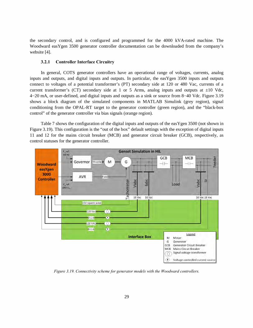
In general, COTS generator controllers have an operational range of voltages, currents, analog inputs and outputs, and digital inputs and outputs. In particular, the easYgen 3500 inputs and outputs connect to voltages of a potential transformer’s (PT) secondary side at 120 or 480 Vac, currents of a current transformer’s (CT) secondary side at 1 or 5 Arms, analog inputs and outputs at ±10 Vdc, 4−20 mA, or user-defined, and digital inputs and outputs as a sink or source from 8−40 Vdc. Figure 3.19 shows a block diagram of the simulated components in MATLAB Simulink (grey region), signal conditioning from the OPAL-RT target to the generator controller (green region), and the “black-box control” of the generator controller via bias signals (orange region).
Table 7 shows the configuration of the digital inputs and outputs of the easYgen 3500 (not shown in Figure 3.19). This configuration is the “out of the box” default settings with the exception of digital inputs 11 and 12 for the mains circuit breaker (MCB) and generator circuit breaker (GCB), respectively, as control statuses for the generator controller.
Figure 3.19. Connectivity scheme for generator models with the Woodward controllers.
30
TABLE 4
Woodward Digital Inputs and Outputs Function Type Configured for Terminal HIL DO HIL DI
0 Common Digital Input n/a 66 20
1 Emergency Stop Digital Input Alarm 67 1
2 Start in Auto Digital Input Control 68 2
3 Low Oil Pressure Digital Input Alarm 69
4 Coolant Temp. Digital Input Alarm 70
5 External alarm acknowledge Digital Input Control 71 3
6 Enable MCB Digital Input Control 72 4
7 Reply MCB is open Digital Input Control 73 5
8 Reply GCB is open Digital Input Control 74 6
9 Discrete input configurable
10 Spare
11 MCB Orange Grey 77 9
12 GCB Yellow Purple 78 10
1 Ready for operation Digital Output n/a 41 1
Power Digital Output n/a 42 0
2 Centralized Alarm (Horn) Digital Output n/a 43 2
3 Starter (Crank) Digital Output n/a 44 3
4 Fuel Solenoid (Fuel Valve) Digital Output n/a 45 4
Power Digital Output n/a 46 0
5 Pre-glow Digital Output n/a 47 5
Power Digital Output n/a 48 0
6 Close GCB Digital Output n/a 49 6
Power Digital Output n/a 50 0
7 Open GCB Digital Output n/a 51 7
Power Digital Output n/a 52 0
8 Close MCB Digital Output n/a 53 8
Power Digital Output n/a 54 0
31
9 Open MCB Digital Output n/a 55 9
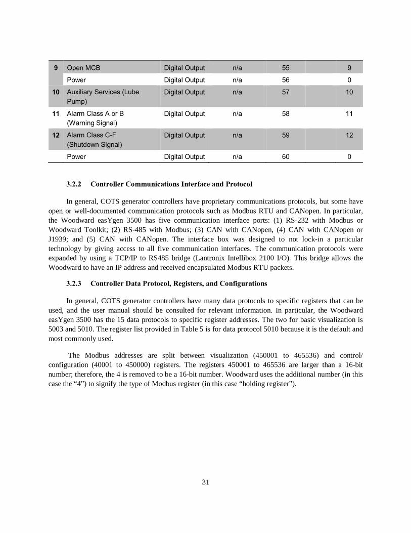
Power Digital Output n/a 56 0
10 Auxiliary Services (Lube Pump)
Digital Output n/a 57 10
11 Alarm Class A or B (Warning Signal)
Digital Output n/a 58 11
12 Alarm Class C-F (Shutdown Signal)
Digital Output n/a 59 12
Power Digital Output n/a 60 0
3.2.2 Controller Communications Interface and Protocol
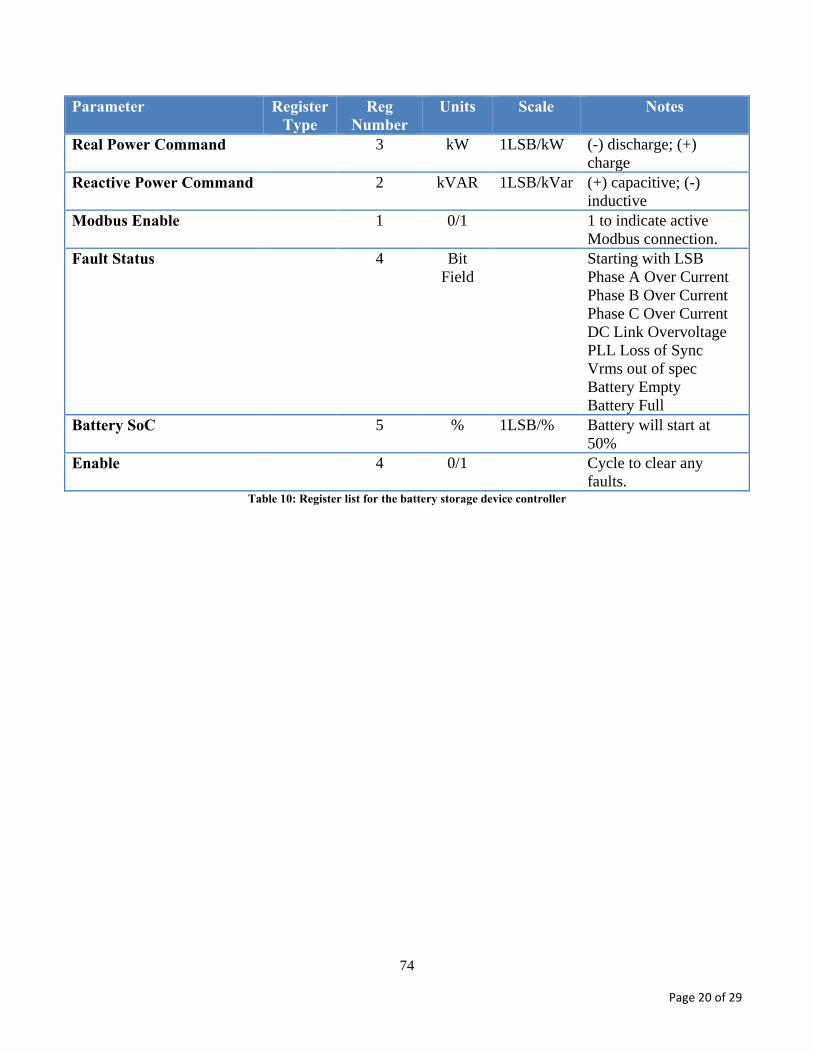
In general, COTS generator controllers have proprietary communications protocols, but some have open or well-documented communication protocols such as Modbus RTU and CANopen. In particular, the Woodward easYgen 3500 has five communication interface ports: (1) RS-232 with Modbus or Woodward Toolkit; (2) RS-485 with Modbus; (3) CAN with CANopen, (4) CAN with CANopen or J1939; and (5) CAN with CANopen. The interface box was designed to not lock-in a particular technology by giving access to all five communication interfaces. The communication protocols were expanded by using a TCP/IP to RS485 bridge (Lantronix Intellibox 2100 I/O). This bridge allows the Woodward to have an IP address and received encapsulated Modbus RTU packets.
3.2.3 Controller Data Protocol, Registers, and Configurations
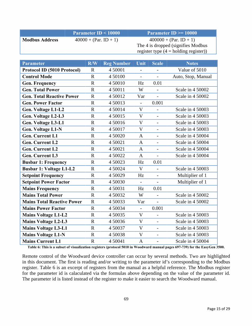
In general, COTS generator controllers have many data protocols to specific registers that can be used, and the user manual should be consulted for relevant information. In particular, the Woodward easYgen 3500 has the 15 data protocols to specific register addresses. The two for basic visualization is 5003 and 5010. The register list provided in Table 5 is for data protocol 5010 because it is the default and most commonly used.
The Modbus addresses are split between visualization (450001 to 465536) and control/ configuration (40001 to 450000) registers. The registers 450001 to 465536 are larger than a 16-bit number; therefore, the 4 is removed to be a 16-bit number. Woodward uses the additional number (in this case the “4”) to signify the type of Modbus register (in this case “holding register”).
32
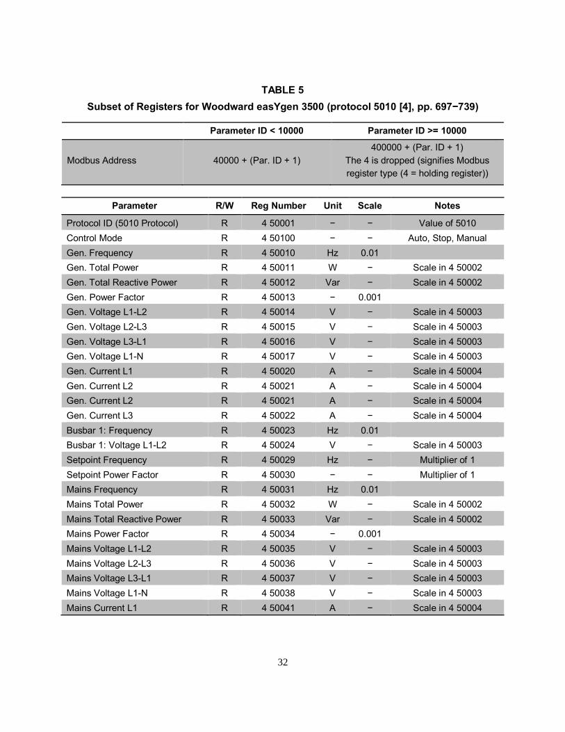
TABLE 5 Subset of Registers for Woodward easYgen 3500 (protocol 5010 [4], pp. 697−739)
Parameter R/W Reg Number Unit Scale Notes
Protocol ID (5010 Protocol) R 4 50001 − − Value of 5010 Control Mode R 4 50100 − − Auto, Stop, Manual Gen. Frequency R 4 50010 Hz 0.01 Gen. Total Power R 4 50011 W − Scale in 4 50002 Gen. Total Reactive Power R 4 50012 Var − Scale in 4 50002 Gen. Power Factor R 4 50013 − 0.001 Gen. Voltage L1-L2 R 4 50014 V − Scale in 4 50003 Gen. Voltage L2-L3 R 4 50015 V − Scale in 4 50003 Gen. Voltage L3-L1 R 4 50016 V − Scale in 4 50003 Gen. Voltage L1-N R 4 50017 V − Scale in 4 50003 Gen. Current L1 R 4 50020 A − Scale in 4 50004 Gen. Current L2 R 4 50021 A − Scale in 4 50004 Gen. Current L2 R 4 50021 A − Scale in 4 50004 Gen. Current L3 R 4 50022 A − Scale in 4 50004 Busbar 1: Frequency R 4 50023 Hz 0.01 Busbar 1: Voltage L1-L2 R 4 50024 V − Scale in 4 50003 Setpoint Frequency R 4 50029 Hz − Multiplier of 1 Setpoint Power Factor R 4 50030 − − Multiplier of 1 Mains Frequency R 4 50031 Hz 0.01 Mains Total Power R 4 50032 W − Scale in 4 50002 Mains Total Reactive Power R 4 50033 Var − Scale in 4 50002 Mains Power Factor R 4 50034 − 0.001 Mains Voltage L1-L2 R 4 50035 V − Scale in 4 50003 Mains Voltage L2-L3 R 4 50036 V − Scale in 4 50003 Mains Voltage L3-L1 R 4 50037 V − Scale in 4 50003 Mains Voltage L1-N R 4 50038 V − Scale in 4 50003 Mains Current L1 R 4 50041 A − Scale in 4 50004
Parameter ID < 10000 Parameter ID >= 10000
Modbus Address 40000 + (Par. ID + 1) 400000 + (Par. ID + 1)
The 4 is dropped (signifies Modbus register type (4 = holding register))
33
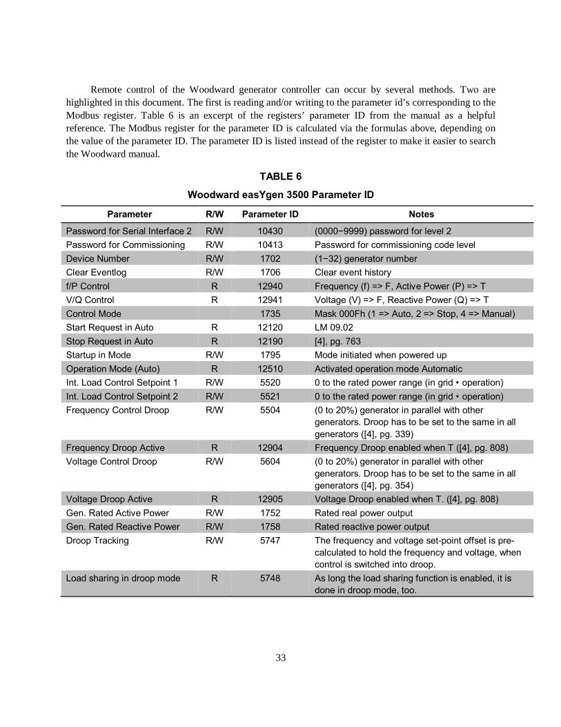
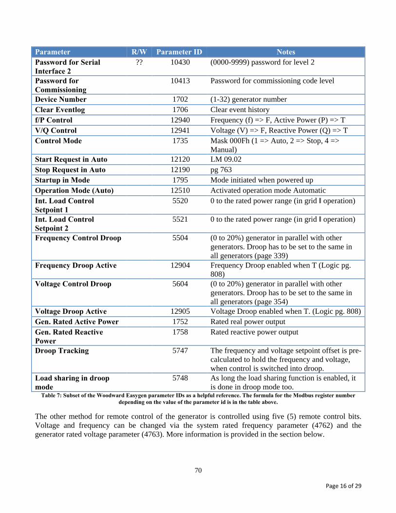
Remote control of the Woodward generator controller can occur by several methods. Two are highlighted in this document. The first is reading and/or writing to the parameter id’s corresponding to the Modbus register. Table 6 is an excerpt of the registers’ parameter ID from the manual as a helpful reference. The Modbus register for the parameter ID is calculated via the formulas above, depending on the value of the parameter ID. The parameter ID is listed instead of the register to make it easier to search the Woodward manual.
TABLE 6
Woodward easYgen 3500 Parameter ID
Parameter R/W Parameter ID Notes
Password for Serial Interface 2 R/W 10430 (0000−9999) password for level 2 Password for Commissioning R/W 10413 Password for commissioning code level Device Number R/W 1702 (1−32) generator number Clear Eventlog R/W 1706 Clear event history f/P Control R 12940 Frequency (f) => F, Active Power (P) => T V/Q Control R 12941 Voltage (V) => F, Reactive Power (Q) => T Control Mode 1735 Mask 000Fh (1 => Auto, 2 => Stop, 4 => Manual) Start Request in Auto R 12120 LM 09.02 Stop Request in Auto R 12190 [4], pg. 763 Startup in Mode R/W 1795 Mode initiated when powered up Operation Mode (Auto) R 12510 Activated operation mode Automatic Int. Load Control Setpoint 1 R/W 5520 0 to the rated power range (in grid • operation) Int. Load Control Setpoint 2 R/W 5521 0 to the rated power range (in grid • operation) Frequency Control Droop R/W 5504 (0 to 20%) generator in parallel with other
generators. Droop has to be set to the same in all generators ([4], pg. 339)
Frequency Droop Active R 12904 Frequency Droop enabled when T ([4], pg. 808) Voltage Control Droop R/W 5604 (0 to 20%) generator in parallel with other
generators. Droop has to be set to the same in all generators ([4], pg. 354)
Voltage Droop Active R 12905 Voltage Droop enabled when T. ([4], pg. 808) Gen. Rated Active Power R/W 1752 Rated real power output Gen. Rated Reactive Power R/W 1758 Rated reactive power output Droop Tracking R/W 5747 The frequency and voltage set-point offset is pre-
calculated to hold the frequency and voltage, when control is switched into droop.
Load sharing in droop mode R 5748 As long the load sharing function is enabled, it is done in droop mode, too.
34
The other method for remote control of the generator was to program the Woodward easYgen 3500 to interface with the MIT LL generator interface document developed in a past sponsored program for open source interfaces. Though this is an open interface, it is not yet currently adopted by all generator manufacturers. In this interface, the generator is controlled using five (5) remote control bits. Voltage and frequency can be changed via the system-rated frequency parameter (4762) and the generator-rated voltage parameter (4763). More information is provided in the section below.
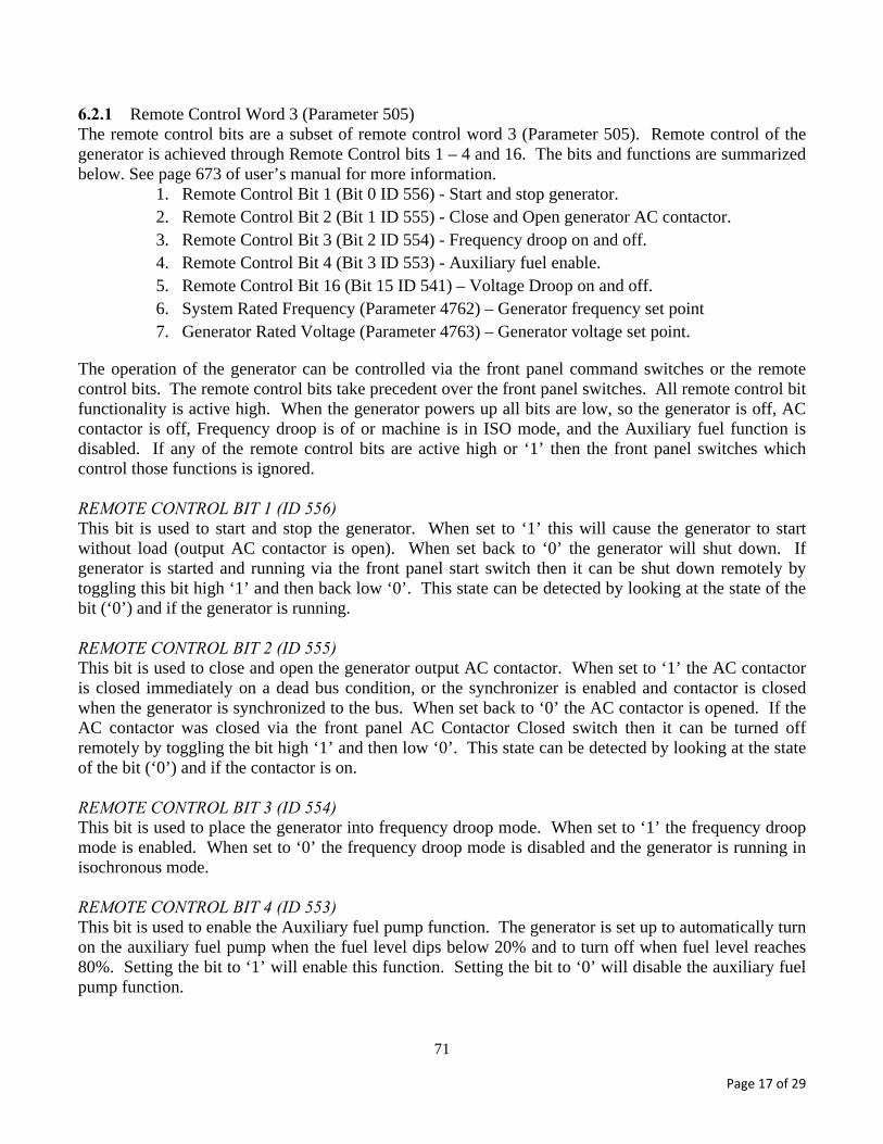
3.2.4 Remote Control Bits and Description
a. Remote Control Word 3 (Parameter 505)
The remote control bits are a subset of remote control word 3 (Parameter 505). Remote control of the generator is achieved through Remote Control bits 1–4 and 16. The bits and functions are summarized below. See page 673 of the user’s manual for more information [4].
1. Remote Control Bit 1 (Bit 0 ID 556) − Start and stop generator.
2. Remote Control Bit 2 (Bit 1 ID 555) − Close and Open generator AC contactor.
3. Remote Control Bit 3 (Bit 2 ID 554) − Frequency droop on and off.
4. Remote Control Bit 4 (Bit 3 ID 553) − Auxiliary fuel enable.
5. Remote Control Bit 16 (Bit 15 ID 541) – Voltage droop on and off.
6. System-Rated Frequency (Parameter 4762) – Generator frequency set point
7. Generator-Rated Voltage (Parameter 4763) – Generator voltage set point.
The operation of the generator can be controlled via the front panel command switches or the remote control bits. The remote control bits take precedent over the front panel switches. All remote control bit functionality is active high. When the generator powers up, all bits are low, so the generator is off, AC contactor is off, frequency droop is off or machine is in ISO mode, and the auxiliary fuel function is disabled. If any of the remote control bits are active high or ‘1’, then the front panel switches that control those functions is ignored.
b. Remote Control Bit 1 (ID 556)
This bit is used to start and stop the generator. When set to ‘1’, this will cause the generator to start without load (output AC contactor is open). When set back to ‘0’, the generator will shut down. If the generator is started and running via the front panel start switch, then it can be shut down remotely by toggling this bit high ‘1’ and then back low ‘0’. This state can be detected by looking at the state of the bit (‘0’) and if the generator is running.
35
c. Remote Control Bit 2 (ID 555)
This bit is used to close and open the generator output AC contactor. When set to ‘1’, the AC contactor is closed immediately on a dead-bus condition, or the synchronizer is enabled and contactor is closed when the generator is synchronized to the bus. When set back to ‘0’, the AC contactor is opened. If the AC contactor was closed via the front panel AC Contactor Closed switch, then it can be turned off remotely by toggling the bit high ‘1’ and then low ‘0’. This state can be detected by looking at the state of the bit (‘0’) and if the contactor is on.
d. Remote Control Bit 3 (ID 554)
This bit is used to place the generator into frequency droop mode. When set to ‘1’, the frequency droop mode is enabled. When set to ‘0’, the frequency droop mode is disabled and the generator is running in isochronous mode.
e. Remote Control Bit 4 (ID 553)
This bit is used to enable the auxiliary fuel pump function. The generator is set up to automatically turn on the auxiliary fuel pump when the fuel level dips below 20% and to turn off when fuel level reaches 80%. Setting the bit to ‘1’ will enable this function. Setting the bit to ‘0’ will disable the auxiliary fuel pump function.
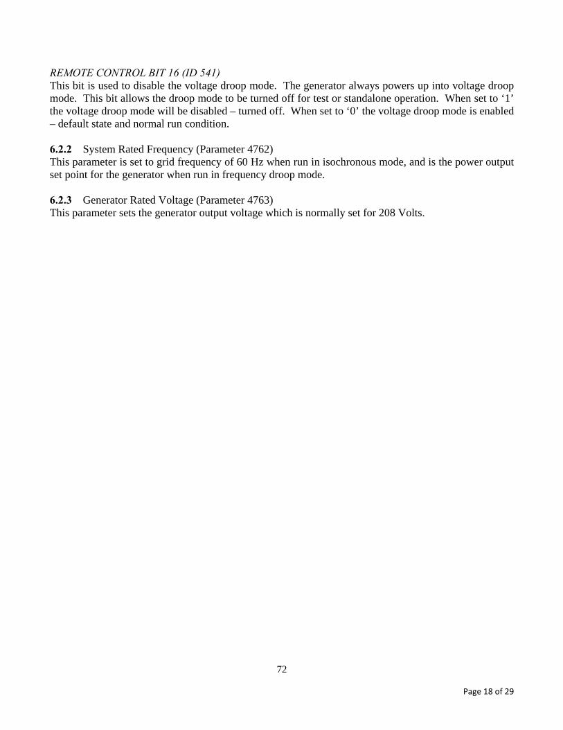
f. Remote Control Bit 16 (ID 541)
This bit is used to disable the voltage droop mode. The generator always powers up into voltage droop mode. This bit allows the droop mode to be turned off for test or standalone operation. When set to ‘1’, the voltage droop mode will be disabled – turned off. When set to ‘0’, the voltage droop mode is enabled – default state and normal run condition.
g. System-Rated Frequency (Parameter 4762)
This parameter is set to grid frequency of 60 Hz when run in isochronous mode, and is the power output set point for the generator when run in frequency droop mode.
h. Generator-Rated Voltage (Parameter 4763)
This parameter sets the generator output voltage, which is normally set for line to neutral voltage.
3.3 FIREWALL SETUP AND CONFIGURATION
MIT Lincoln Laboratory implemented a firewall in the Hardware-in-the-Loop (HIL) Platform system architecture for administrative and research purposes. It was used to characterize the network and cybersecurity posture. The firewall was used administratively to maintain separation (different subnets) of
36
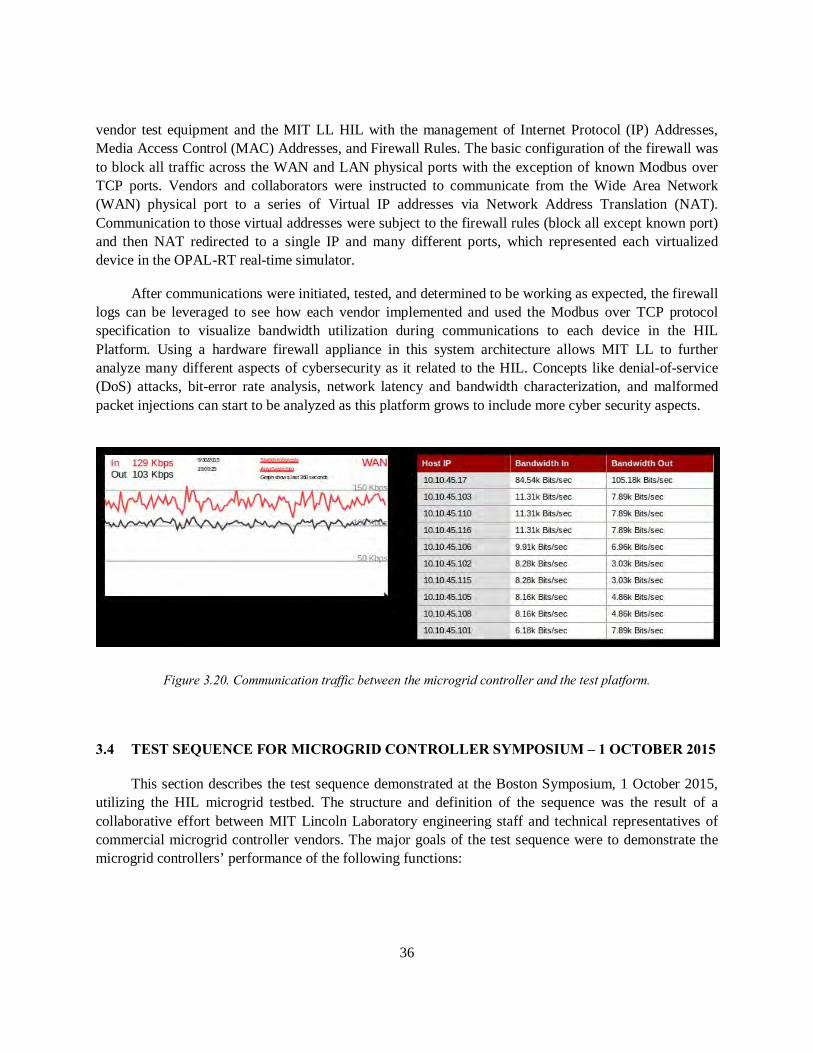
vendor test equipment and the MIT LL HIL with the management of Internet Protocol (IP) Addresses, Media Access Control (MAC) Addresses, and Firewall Rules. The basic configuration of the firewall was to block all traffic across the WAN and LAN physical ports with the exception of known Modbus over TCP ports. Vendors and collaborators were instructed to communicate from the Wide Area Network (WAN) physical port to a series of Virtual IP addresses via Network Address Translation (NAT). Communication to those virtual addresses were subject to the firewall rules (block all except known port) and then NAT redirected to a single IP and many different ports, which represented each virtualized device in the OPAL-RT real-time simulator.
After communications were initiated, tested, and determined to be working as expected, the firewall logs can be leveraged to see how each vendor implemented and used the Modbus over TCP protocol specification to visualize bandwidth utilization during communications to each device in the HIL Platform. Using a hardware firewall appliance in this system architecture allows MIT LL to further analyze many different aspects of cybersecurity as it related to the HIL. Concepts like denial-of-service (DoS) attacks, bit-error rate analysis, network latency and bandwidth characterization, and malformed packet injections can start to be analyzed as this platform grows to include more cyber security aspects.
Figure 3.20. Communication traffic between the microgrid controller and the test platform.
3.4 TEST SEQUENCE FOR MICROGRID CONTROLLER SYMPOSIUM – 1 OCTOBER 2015
This section describes the test sequence demonstrated at the Boston Symposium, 1 October 2015, utilizing the HIL microgrid testbed. The structure and definition of the sequence was the result of a collaborative effort between MIT Lincoln Laboratory engineering staff and technical representatives of commercial microgrid controller vendors. The major goals of the test sequence were to demonstrate the microgrid controllers’ performance of the following functions:
37
1. Unit commitment (grid-tied and islanded)
2. Peak-shaving, valley-filling, and load-shedding (grid-tied and islanded)
3. Diesel generation fuel optimization (grid-tied and islanded)
4. Loss minimization (islanded)
5. Meet power export requirements (grid-tied)
6. Optimized energy-storage control (grid-tied)
7. Generator-battery hybridization (grid-tied)
8. Power factor support at PCC (grid-tied)
9. Two-way communication with commercial generator controllers (grid-tied and islanded)
Note: The functions of optimized energy-storage control and generator-battery hybridization were only performed during grid-tied because of the inadequate simulated model for the battery controller. A commercial controller would be required for proper evaluation.
In order to expedite execution of the HIL demonstration at the Symposium, the test sequence was shortened from a planned duration of 2 hours to a duration of 15 minutes so that all Symposium attendees would have an opportunity to view the full demonstration. The profiles discussed in the following subsections consist of 15-minute data segments followed by a 15-minute “mirrored” data, such that simulations run continuously without drastic and unrealistic system changes. However, only the first 15 minutes of simulation are used for data analysis.
3.4.1 Load Categories and Available Generating Capacity
The microgrid serves ten loads with the assigned categories shown in Table 7. The actual demand curves for these loads are shown in the Section A.2. Due to the short development timeline (approximately 3 months), the large induction motors (see Figure 3.1) were modeled as static loads for the Symposium test sequence. However, future work will include the evaluation of the microgrid controller’s load balancing during on/off switching of large motors.
38
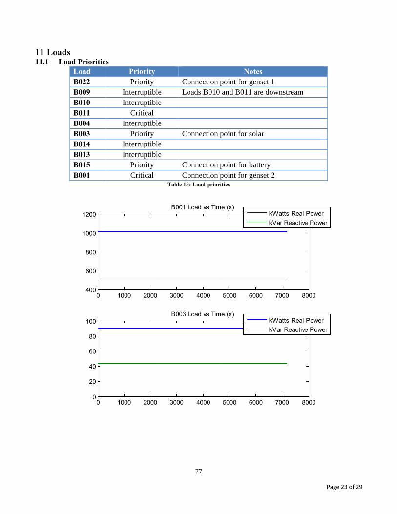
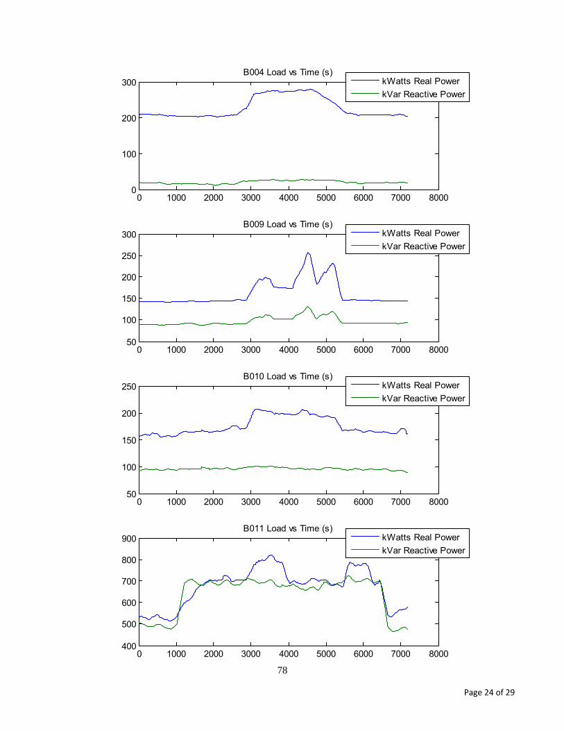
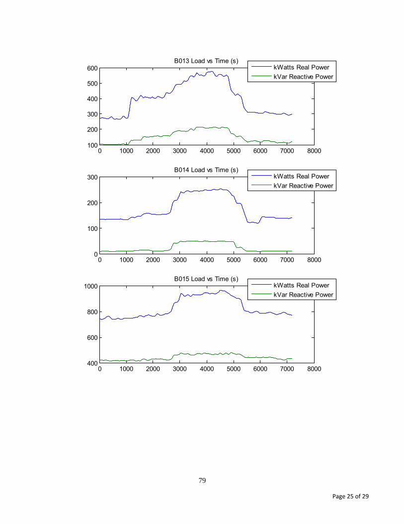
TABLE 7 Load Categories
Load Priority Notes
B022 Priority Static load. Connection point for the 4 MVA genset
B009 Interruptible Dynamic load. B010 and B011 are downstream
B010 Interruptible Dynamic load
B011 Critical Dynamic load
B004 Interruptible Dynamic load
B003 Priority Static load. Connection point for the PV system
B014 Interruptible Dynamic load
B013 Interruptible Dynamic load
B015 Priority Dynamic load. Connection point for the 4 MVA ESS
B001 Critical Static load. Connection point for the 1 MVA genset The generation capability of the microgrid comprises a 1 MVA generator (G1), a 4 MVA generator
(G2), a 3.5 MW PV array, and an ESS capable of sourcing 4 MVA. The detailed characteristics of these sources are covered elsewhere in this report. During the test sequence, the generators are continuously available to the microgrid controller to support operations such as peak-shaving and exporting. The availability of the PV array and the ESS was restricted to grid-tied operations due to limitations associated with the inverter controller model that was used as a component of the ESS and PV system models. Future work will include the integration of commercial controllers for these components, enabling their use during islanded conditions. The irradiance profile used for the PV array is given in Section A.3. This profile was generated by applying a decimation/interpolation filter to the signal from a solar flux point detector to approximate the spatially averaged output of a PV array.
3.4.2 Test Sequence Timeline Events – Vendor 1
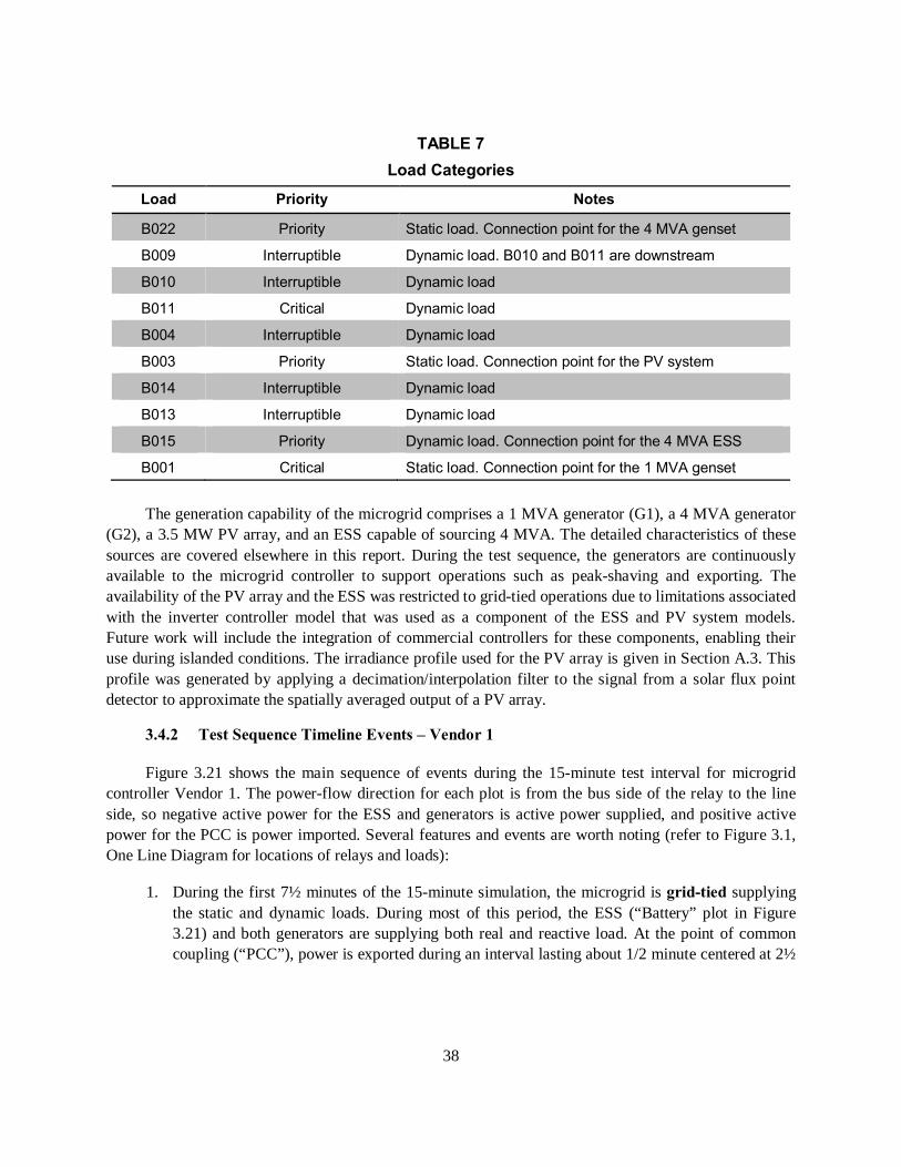
Figure 3.21 shows the main sequence of events during the 15-minute test interval for microgrid controller Vendor 1. The power-flow direction for each plot is from the bus side of the relay to the line side, so negative active power for the ESS and generators is active power supplied, and positive active power for the PCC is power imported. Several features and events are worth noting (refer to Figure 3.1, One Line Diagram for locations of relays and loads):
1. During the first 7½ minutes of the 15-minute simulation, the microgrid is grid-tied supplying the static and dynamic loads. During most of this period, the ESS (“Battery” plot in Figure 3.21) and both generators are supplying both real and reactive load. At the point of common coupling (“PCC”), power is exported during an interval lasting about 1/2 minute centered at 2½
39
minutes into the simulation and again for about 1½ minutes at 4 minutes into the simulation. During both of these segments, the ESS and both generators are supplying active and reactive power, and the microgrid is also supplying net active and reactive power to the grid.
2. At 7½ minutes, the microgrid controller sheds loads B004, B009, B010, and B022, a total of about 3.5 MW. In addition, the microgrid controller opens R12 to island the PV source and the ESS. (This action was taken to allow the simulation to continue to run without crashing through the islanded segment as described elsewhere in this report.) As a result of R12 opening, the current-source inverters associated with the PV and ESS cause an overvoltage trip on relays R13 (ESS relay), R14 (load B015 relay), R15 (load B013 relay), and R16 (B014 relay). Load B015 is subsequently reconnected at about 8 minutes, shortly before the microgrid controller islands the microgrid from the grid. However, since relays R12 (grid), R17 (PV), and R13 (ESS) are all open, there is no available source to pick up the load.
3. At about 8.3 minutes into the simulation, the microgrid controller opens relay R1 and islands the microgrid. During the islanded period, the two gensets supply the connected load (B004, B009, B010, and B011, as well as both 250 horsepower motors). The PV and the ESS are disconnected during islanded mode to avoid stability problems caused by the inadequate controller model.
40
Figure 3.21. Power flow through PCC, generators, and battery – Vendor 1.
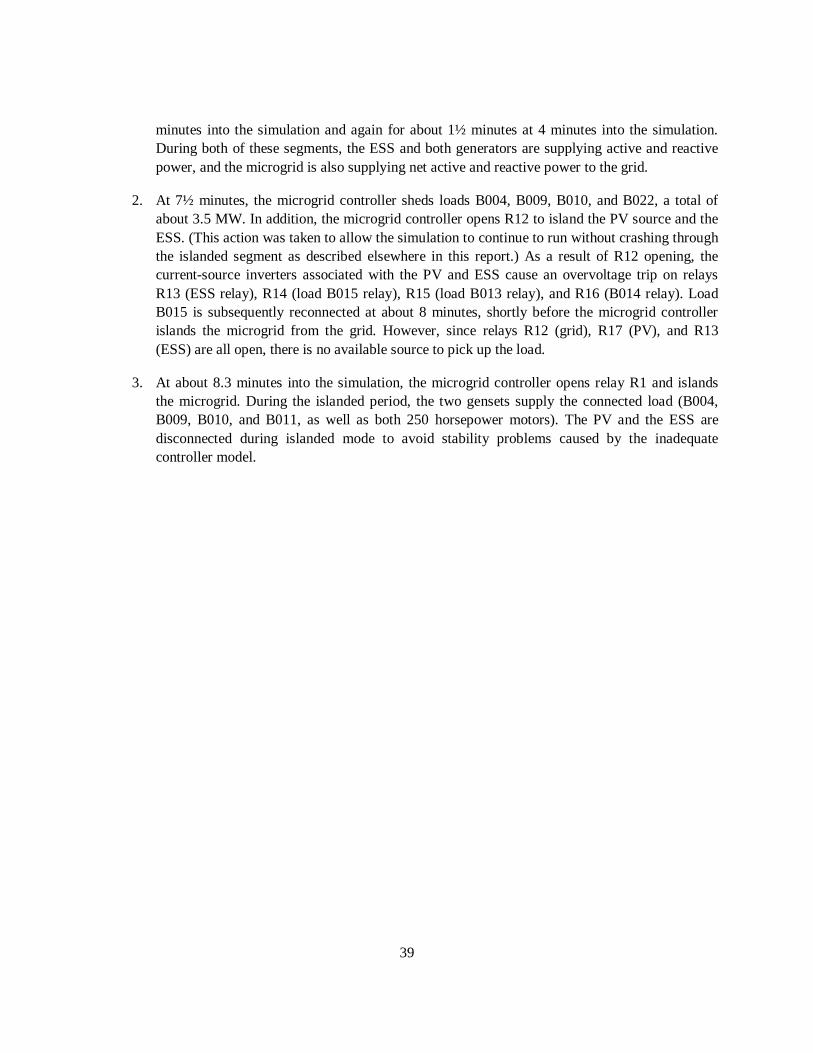
3.4.3 Test Sequence Timeline Events – Vendor 2
Figure 3.22 illustrates the main sequence of events for Vendor 2. While the major features of load export, import, and islanding are similar to the corresponding events for Vendor 1, there are a few salient differences between the two sequences, which are evident in the plots. Vendor 2 imports heavily from the grid early on in the sequence and ramps up the genset loads after about 2½ minutes into the test, while Vendor 1 drew more heavily from the grid just before islanding. Vendor 2 uses the ESS to supply real
41
power after about 4 minutes until islanding occurs near 7½ minutes into the test. In addition, Vendor 2 does not attempt to shed load prior to islanding, which may contribute to the large spikes in power that occur on the generator buses when the microgrid transitions to the islanded condition.
Loads B009 and B010 are removed at the transition to islanded operation but are reconnected after about 1/2 minute as shown in the traces in the lower right of Figure 3.22. It also appears that Vendor 2 did not attempt to supply as much reactive power back to the grid from the ESS as Vendor 1 appears to have done during a segment near 5 minutes into the test. Also, both Vendor 1 and Vendor 2 experience large reactive power absorption on genset 2 at the end of the simulation during islanded mode. This is due to the large capacitance associated with a stub line in the model that is required for numerical stability.
Figure 3.22. Power flow through PCC, generators, and battery – Vendor 2.
This page intentionally left blank.
43
4. RESULTS FROM FIRST SYMPOSIUM
4.1 EVALUATION METRICS FOR MICROGRID CONTROLLER
One of our main objectives with the HIL platform was for it to enable vendors to demonstrate their products’ capabilities, differentiate working functionality from marketing “vaporware,” and set themselves apart from their competition with hard performance metrics. The Microgrid Controller Symposium event brought together a wide spectrum of stakeholders in the microgrid community to witness a demonstration of the power and potential of hardware-in-the-loop technology for the purpose of
1. Demonstrating and showcasing the features and capabilities of the microgrid controller hardware that is currently being offered by manufacturers
2. Eventual cost-effective application as a commissioning platform for microgrid deployment
3. Eventual application as a validation platform for vendors, test laboratories, and utilities to verify standards compliance
The Symposium was a great success in this regard, as evidenced by the high level of attendance by utility companies, project developers, system integrators, and manufacturers, as well as their active participation at the HIL demonstration.
It should also be emphasized that the HIL demonstration itself was not intended to simulate a flawlessly operating microgrid and microgrid controller, but instead the intent was to show how HIL technology can be used to provide a cost-effective and highly accessible path to the design, development, and eventual implementation of a microgrid. In this respect, the HIL technology demonstration provided a glimpse into how the technology can be used as a vehicle to achieve a fast, cost-effective, and robust design process for microgrid development.
The subsection below describes the evaluation metrics proposed for microgrid controller performance evaluation and summarize the findings from data generated at the Symposium.
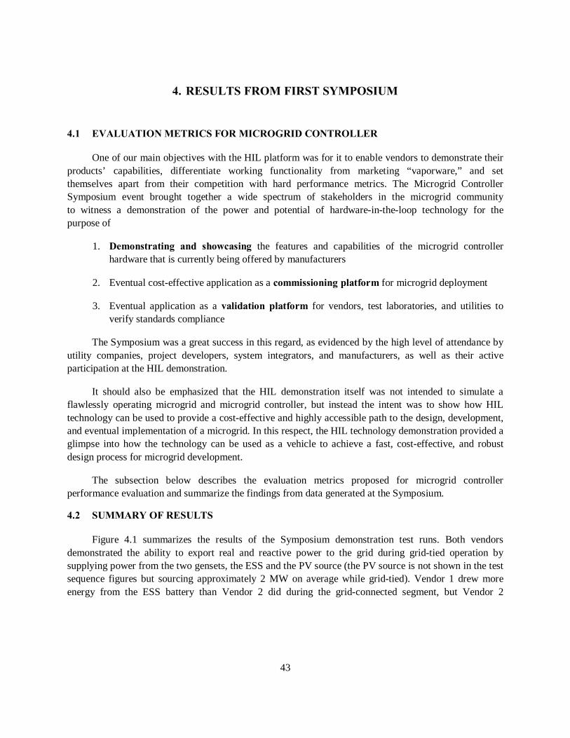
4.2 SUMMARY OF RESULTS
Figure 4.1 summarizes the results of the Symposium demonstration test runs. Both vendors demonstrated the ability to export real and reactive power to the grid during grid-tied operation by supplying power from the two gensets, the ESS and the PV source (the PV source is not shown in the test sequence figures but sourcing approximately 2 MW on average while grid-tied). Vendor 1 drew more energy from the ESS battery than Vendor 2 did during the grid-connected segment, but Vendor 2
44
maintained load on the two gensets for a longer period of time, which resulted in the higher fuel usage for Vendor 2, as shown in Figure 4.1.
Since Vendor 2 transitioned to the island configuration about a minute earlier than Vendor 1 did, the load demands shown in the lower-left table in Figure 4.1 are higher for Vendor 2. Due to the aforementioned issue with model stability, a significant fraction of the priority loads (including B003 and B015) could not be carried during islanded mode. However, both vendors carried the critical loads through the islanding operational period.
Figure 4.1. Anonymized results of microgrid controller demonstration cases.
45
5. INTEGRATION WITH VENDORS: CHALLENGES AND LESSONS LEARNED
Several challenges were encountered during the “first-time-through” process of integrating the vendor microgrid controllers with the HIL system. The difficulties encountered were neither unexpected nor insurmountable, but a significant amount of time and effort was required to overcome them. The integration process had to be repeated for the second vendor’s microgrid controller, and this second integration process went more smoothly than the first, which is encouraging for future efforts. Listed in the paragraphs below are several challenges that were encountered, along with the resulting lessons learned/recommended actions necessary to address them. Implementation of these measures will take time and effort, but will enhance the overall HIL integration process for future test and evaluation campaigns.
One particular challenge encountered was the need for the microcontroller vendors to gain familiarity with certain aspects and features of model components that played a role in system-level microgrid operation. To address this challenge, more thorough documentation of the underlying models will likely accelerate the integration and test time. Model documentation can be included right in the baseline model where special considerations need to be mentioned. Furthermore, building subsystem level models that test many aspects and features of components would be helpful because it proves out the design and would give potential users an example of how the subsystem should be used and which areas are tested.
The heads-up display is a crucial piece of the HIL system. It serves as the central graphical interface for monitoring simulated microgrid operation during execution of the simulation, but it can also provide vital details during integration testing. Lack of visibility into the system when a vendor is controlling sub-components can make troubleshooting more difficult. Additional displays for each component would be helpful to give insight into lower-level details. This could take the form of exported data or Simulink scopes, which are organized to cleanly present all the useful component details.
Perhaps the greatest challenge associated with vendor integration for the first symposium was to overcome initial problems in achieving reliable and functional Modbus communications between the vendor microgrid controller hardware and the OPAL-RT HIL simulator system. Several suggestions that are being implemented will make this process more straightforward in the future. First, Lincoln Laboratory is setting up a provision for remote access to the HIL system to provide vendors the ability to test microgrid controller functionality from the comfort of their own laboratory. This remote access will provide heads-up display-type details on a webpage. Any other test methods that make access to the HIL system more easily attained would also be helpful. The one hardware unit was often a bottleneck as Lincoln Laboratory personnel and vendors both competed for test time. A separate piece of hardware, such as a Modbus simulator with sufficient fidelity to emulate the HIL Modbus interface, could be utilized to great advantage for this non-real-time communication debug phase, but would likely
46
require time and effort to implement. In addition, improvements and clarifications to the HIL Modbus interface definition would also help. If necessary, a formal interface control document (ICD) could be written. Modbus was selected because it is one of the easier methods of communication, but it has drawbacks. Extra debug time was needed to resolve inconsistent register functions between devices. Common Modbus interface standards for devices like generators, batteries, or PV would reduce this integration and debug time. One example is a consistent sign convention on the direction of power flow relative to the position (upstream/downstream) from the PCC. Where possible, we tried to make upstream flow from a component to the PCC a positive number. From what we’ve seen even when a family of controllers is supported by a microgrid controller, there are still a myriad of interface registers that could be used to achieve the desired results. Some may not even be correctly documented. Simple models to debug communication and corresponding component displays would make this process faster. Lastly, Modbus is a relatively insecure communication standard, as all commands are sent through unencrypted TCP connections. With these comments in mind, it may make sense to consider other protocols. That being said, the challenge is finding a common standard that vendors are ready to support for a range of devices today.
Some challenges that were encountered were related to debugging subsystem-level issues at the system level. Overall, the philosophy that should be used during integration is “test small and demo big.” Each piece needs to be carefully taken through its operation before the next is added. Identifying three issues in a large system is much more challenging than identifying the same three issues in smaller systems. When the time comes for integration of all the pieces, new concerns will arise, but at least the others are not further clouding the understanding of the larger system. Once all the integration issues are worked out, the question of whether the microgrid controller is controlling the grid in an optimal, robust, or efficient way can be addressed. This may still require various test sequences for each microgrid function test. It may also require more simulation time for realistic load profiles, unit commitment, and other temporal effects to be properly represented.
47
6. RECOMMENDATIONS FOR TEST PROCEDURES AND EVALUATION METRICS
The value of hardware-in-the-loop simulation is strongly influenced by the realism of the modelled components and procedures represented. To this end, the following suggestions are made to enhance both simulation fidelity and procedural relevance (much of this content was extracted from the questionnaire responses received at the Symposium):
1. Include edge cases (e.g., line-line and line-ground faults and other off-nominal conditions) as part of the simulation environment and test cases
2. Focus more on dynamic islanded operation
3. Integrate higher fidelity distributed energy resource (DER) controllers
4. Integrate distribution management systems
5. Evaluate to industry standards
6. Incorporate cybersecurity features and test their effectiveness
7. Incorporate self-healing and configurability into the simulated microgrid
8. Simulate the influence the ISO energy market would have on microgrid operation
The benefit of producing HIL testing results that are traceable to industry standards is an important goal that will accelerate the acceptance of the HIL technology for cost-effective microgrid development. Some of the important parameters to compare when evaluating relative microgrid controller performance metrics include
1. Energy sourced by renewables such as PV
2. Gallons of fuel used or other hydrocarbon consumption
3. Net energy (imported–exported)
4. Peak-shaving and valley-filling performance
5. Power factor correction performance
6. Dynamic islanding stability
7. Fault isolation and recovery
8. Voltage and frequency stability
48
The gross energy sourced by renewables is an obvious metric for comparison. For a given load, it is directly related to net energy drawn from the grid, as well as to peak-shaving performance. An effective dispatching strategy would maximize renewable sources over consumable (e.g., diesel) sources, but peak shaving capability relies on both types of sources, and therefore all three metrics (energy sourced by renewables (kWh), energy sourced by consumables (gallons of fuel), and peak-shaving (kWh)) need to be compared as a group when determining relative effectiveness in energy management. Reactive power management can be provided by renewable generating sources as well as rotating sources, so power factor correction performance comparisons should also take into account the distribution of sources (renewable vs. consumable) used to supply the kVAr required. The ability of the microgrid controller to isolate faults and reconfigure the distribution network to maximize load served can be measured by comparing the load-not-served (LNS) metric directly for different load categories (e.g., critical, priority, and interruptible). Similarly, the voltage and frequency stability of the microgrid can be measured by comparing the durations for which frequency or voltage exceeds standard tolerances, e.g., 5% of nominal values.
49
7. RECOMMENDATIONS FOR NEXT SYMPOSIUM
General recommendations for the next symposium are in line with the responses that were received to the questionnaire filled out by the Symposium participants. Some of the major recommendations are:
1. Improve relevance and realism of HIL testing, to include
a. Fault conditions
b. More dynamic islanding
c. Integration of more DER devices, as well as distribution management systems
2. Increase participation of symposium attendees, including
a. Attendee-contributed test cases
b. Attendee-contributed reference feeders
c. Attendee-contributed residential microgrid concepts and advanced ESS dispatch optimizations
The feedback also highlighted the structure of the Symposium to be well-organized, especially the coordinated timing between presentations, panel discussions, and real-time demonstrations. If possible, this general symposium format should be maintained for future events.
This page intentionally left blank.
51
APPENDIX A
This section provides some of the details and input data required to recreate the sequences demonstrated during the Boston Symposium, 1 October 2015. These include load profiles, irradiance profile, Woodward controller’s hardware interface, and IP Address mapping.
A.1 WOODWARD INTERFACE DIAGRAM
The current connectivity of equipment, as well as their method of communication, is shown in Figure A.1. As of now, the team successfully implemented two commercially available generator controllers. Future work envisions a larger number of hardware device controllers, including PV-board, ESS controllers, commercial relays, and different vendor generator controllers, among other components.
Figure A.1. Woodward interface block diagram.
52
A.2 LOAD PROFILES
The demand profile for each of the ten loads used in the HIL demonstration is given in Figure A.2. The profiles discussed consist of 15-minute data segments followed by a 15-minute “mirrored” data such that simulations run continuously without drastic and unrealistic system changes. It is important to note that the demand from critical loads B001, B003, and B022 have a nearly constant profile. However, the other loads in the system demonstrate a more dynamic behavior.
Figure A.2. System loads − demand profile.
A.3 IRRADIANCE PROFILE
Figure A.3 provides the irradiance profile supplied to the PV system during the demonstration. The solar irradiance profile discussed consists of 15-minute data segments followed by a 15-minute “mirrored” data such that simulations run continuously without discontinuities. The curve shown was the result of applying a decimation/interpolation filter to the solar irradiance measured by a point detector. It
0 5 10 15 20 25 30100
150
200
250
300
B00
1
Loads vs. Time (kW, Blue and kVAr, Red)
0 5 10 15 20 25 300
20
40
60
80
B00
3
0 5 10 15 20 25 300
100
200
300
B00
4
0 5 10 15 20 25 3050
100
150
200
B00
9
0 5 10 15 20 25 3050
100
150
200
250
Time (min)
B01
0
0 5 10 15 20 25 30650
700
750
800
850
B01
1
Loads vs. Time (kW, Blue and kVAr, Red)
0 5 10 15 20 25 300
200
400
600
B01
3
0 5 10 15 20 25 300
100
200
300B
014
0 5 10 15 20 25 30400
600
800
1000
B01
5
0 5 10 15 20 25 301000
1500
2000
2500
3000
Time (min)
B02
2
53
is assumed that such a temporal filter will provide a reasonable approximation to the spatially averaged irradiance characteristic, which would be expected from a 2D PV array.
Figure A.3. Solar irradiance profile.
A.4 IP ADDRESS MAPPING
The microgrid controller under test communicates to various interfaces of the device controller and HIL unit. Register lists for each device are provided in the device’s respective section. Note: the connection to the various devices were tested and validated through the firewall.
Time (min)
0 5 10 15 20 25 30
Irrad
ianc
e (W
/m2
)
0
200
400
600
800
1000
1200Solar Irradiance Profile (W/m 2
)
54
Device IP Address TCP Port
Modbus Address Notes
1 MVA Genset Controller 192.168.10.35 502 N/A -
4 MVA Genset Controller 192.168.10.36 502 N/A -
Storage Controller 192.168.10.40 502 N/A -
PV Controller - - - No interface
Relay 1 10.10.45.101 502 N/A Point of Common Coupling
The following document was the only integration information provided to the microgrid controller vendors prior to their arrival on-site for integration with the HIL platform.
Hardware in the Loop Microgrid Controller Information Packet
V1.0
September 21, 2015
55
Page 2 of 29
Revision History
Rev Date Description Editor 0.3 5/29/2015 Introduction and initial survey sent to vendors Nowocin, Smith 0.4 6/10/2015 Described objectives and follow-on plans
Clarified ISO market participation demonstration HIL platform diagram: removed unused interfaces Test feeder diagram: simplified; added relay/sensor locations Added placeholders for Modbus device list, register lists, device parameters, load priorities, and general site info Replaced “SCADA interface” with Modbus-addressed relays Added “Market Interface” and “Physical Setup”
Limpaecher
0.5 6/15/2015 Added Modbus register list for the protection relay Dowdle 0.6 6/16/2015 Updates to Test Setup and Feeder diagrams, added subset of Modbus
register list for the Woodward device controller, and added the load priorities
Nowocin
0.7 8/5/2015 Added Modbus device IP addresses and TCP ports (Table 2) Added genset parameter list (Table 6) and descriptions Added load profile and PV profile (Figure 1) Added genset ratings (section 6.1) Added PV and storage device ratings (sections 7.1, 8.1) Defined relay settings (Table 11) Listed device control modes (Table 4) Clarified demonstration narrative (section 2) Added feeder block diagram (Figure 6) Added detailed one-line diagram, with motors (Figure 7) Added section for the test plan (section 2) Updated relay register numbers (Table 12)
0.8 8/20/2015 Added load profile graphs Battery register list updated Modbus adjusted to reflect IP based addressing instead of ports Starting conditions added
Smith
0.9 8/27/2015 Updated Figure 3 Test Setup to show equipment Updated Figure 3 Test Setup to show interfaces Added Figure 2 Test Setup Rack Updated Figure 2 Test Setup Rack Updated Table 4’s TBD values Explained Figure 4: Fuel Curve (other figures renumbered) Clarified Woodward Modbus additional numbers Added Table 6: Subset of Modbus control registers (other tables are
1.0 9/23/2016 Updated Table 5 with Protocol 5010 addresses which are more common than the 5003 protocol addresses
Nowocin
56
Page 3 of 29
Table of Contents REVISION HISTORY........................................................................................................................................................... 2
TABLE OF CONTENTS ........................................................................................................................................................ 3
5 CONTROL CAPABILITIES ........................................................................................................................................ 12
7 SOLAR PV ARRAY AND INVERTER .......................................................................................................................... 19
14 POINTS OF CONTACT ............................................................................................................................................ 29
57
Page 4 of 29
1 Introduction Microgrids can be used to decrease customer energy costs while increasing resiliency to power grid outages, but the design and construction of these systems is often too expensive. The microgrid controller stands out as one component with widely varying capabilities, levels of maturity, and project-specific integration costs among different vendors. Incompatibility between components and vendors is another concern.
The Department of Homeland Security (DHS) Science and Technology Directorate (S&T), Resilient Systems Division and the Department of Energy (DOE) Office of Electricity are interested in addressing these challenges by developing a microgrid controller hardware-in-the-loop (HIL) platform for the following purposes:
Objective 1: Provide a Demonstration Platform for microgrid controller vendors to showcase their capabilities to entities considering the deployment of microgrids – utility companies, project developers, and systems integrators – at a Microgrid Controller Symposium in Boston.
Objective 2: Provide a Commissioning Platform for an actual microgrid deployment at the Boston Marine Industrial Park (BMIP). The HIL system will integrate the site’s actual device controllers and DMS systems and enable utility risk reduction commissioning and provide test coverage of edge conditions and dangerous fault conditions, thereby reducing eventual hardware commissioning time,
Objective 3: Provide a Validation Platform for vendors, test labs, and utilities to verify conformance with IEEE P2030.7 and P2030.8 microgrid controller functional and test standards once they are completed.
For objective 1, DHS S&T and DOE are coordinating an exposition of several microgrid controllers during the Microgrid Controller Symposium, held at District Hall in Boston on October 1, 2015. Major investor-owned utilities, microgrid project developers, regulators, and systems integrators will be in attendance. The centerpiece of this Symposium is a live operational demonstration of commercial microgrid controllers running in real time.
These controllers will be demonstrated using the hardware in the loop (HIL) system which will simulate a small microgrid and its energy resources. A typical scenario will be exercised and the microgrid controllers will demonstrate operation of the small microgrid. This document outlines the microgrid HIL system, the interfaces, and functional demonstration scenarios.
This information packet will continue to be updated as the design is refined.
58
Page 5 of 29
2 Microgrid Controller Demonstration Sequence The microgrid controller demonstration sequence is categorized into (1) grid-connected, (2) islanded, (3) cybersecurity, and (4) faults. Each of these categories has a narrative with various tests.
The key inputs to the demonstration sequence are (see Figure 1): • Load category
o Critical, priority, or interruptible loads• Demand profile for each load
o Real and reactive power• Large induction motor full voltage start events• Irradiance profile and the corresponding PV array power output• Status of the upstream distribution system / power grid• Power export commitments• Switching events (loss of grid due to external failure)• Fault events [no faults, other than the grid failure, are included in this demonstration sequence]
To create the load profile, eight (8) hours of load data were gathered using smart metering equipment. In the interest of time, however, these data were compressed into 2 hours of demonstration time. Therefore, 15 minutes of test time corresponds to one (1) hour of load activity.
The irradiance data and the corresponding PV power output, however, are uncompressed. One hour of real-time summer irradiance data were gathered. The irradiance data are unmodified during the grid-connected portion of the demonstration (1st hour) and repeated and scaled down during the grid outage (2nd hour). [Some modifications to this profile are still necessary to remove the sharp step change seen at the 1-hour mark in Figure 1.]
Table 1: Target PCC power characteristics during the demonstration sequence
59
Page 6 of 29
Figure 1. 2-hour demonstration sequence
2.1 Grid Connected Demonstration Plan 2.1.1 Narrative Part 1 On a sunny summer afternoon, the microgrid system is working well in a grid tied mode. Loads are coming and going with small spikes occasionally. The microgrid is under a day-ahead contract to export power to the regional ISO market, defined by Table 1 and shown in Figure 1. The microgrid controller should maintain as close to unity power factor at the PCC as possible.
60
Page 7 of 29
Clouds have been forecasted, as well as a severe storm later in the day. After about 15 minutes, the clouds roll in and cause the PV output to fluctuate significantly. When not under obligation to export power, the microgrid controller detects and minimizes demand peaks, particularly the peak caused by a motor start event near the end of the hour. At the end of the first hour, the weather becomes stormy. The PV output decreases significantly and microgrid performance must be adjusted to make up for the change in power produced.
2.1.2 Functionality Demonstrated • Unit commitment• VAR and power factor support• Peak shaving and valley filling• Generator-battery hybridization for reduction of fuel consumption• Preparation for unexpected islanding operation (maintenance of sufficient storage reserves)
2.2 Island Demonstration Plan
2.2.1 Narrative Part 2 The system has stabilized, but lightning strikes in the distance. The local feeder to the microgrid is knocked out. The microgrid controller should island at this time to maintain some level of service to its critical and priority loads. After islanding there is still plenty of demand at the test feeder. In order to maintain power balance with the critical and priority loads, the microgrid controller will likely have to shed the interruptible loads, based on the load priorities provided in Table 13. The microgrid controller will have to maintain sufficient spinning reserve to handle a second motor start soon after the grid outage event.
Sometime later clouds clear and PV output is back to normal levels. Shedded loads can be brought back online to restore near-normal operating conditions on the microgrid. The microgrid remains islanded for the rest of the hour to verify stable power from the grid, and then reconnects after some time.
2.2.2 Functionality Demonstrated • Unit commitment and spinning reserve regulation• Maintenance of voltage and frequency stability within utility tolerances• Load prioritization and load shedding• Control and optimizing energy storage• Generator-battery hybridization and minimization of fuel consumption
2.3 Cybersecurity 2.3.1 Narrative Part 3 Communications between all devices on the Modbus TCP network will be logged and visualized by MIT Lincoln Laboratory (MIT-LL). No penetration tests will be performed for this demonstration.
2.3.2 Functionality Demonstrated • Network activity and bandwidth requirements
2.4 Faults No faults – other than the grid failure – are included in this demonstration sequence.
61
Page 8 of 29
3 HIL Platform Setup and Integration Verification MIT-LL will work with microgrid controller vendors to verify their connectivity to the HIL system several weeks before the scheduled demonstration date. Basic checks for communication between different microgrid components will be verified so that the intended operation of the microgrid will be achieved according to the microgrid controller’s desired strategy.
To maximize the likelihood of a successful demonstration, vendors will first perform integration and testing at MIT-LL prior to the Symposium. The Massachusetts Clean Energy Center (MassCEC) will down-select from those vendors who are successful and wish to proceed to the live Symposium demonstration.
MIT-LL will provide three (3) days of on-site integration of each vendor’s microgrid controller at MIT-LL in Lexington, MA. Upon successful integration, MIT-LL and the vendor will execute a 1-2 hour scripted data collection. For those vendors that experience issues, an additional two (2) days of integration will be made available for vendors to make necessary adjustments and re-test. Note that U.S. citizens or green card holders only are permitted on-site at MIT-LL. MIT-LL engineering resources and HIL platform will be provided on-site at no cost to the vendors; vendors must cover the travel, labor, equipment, and related costs for their own resources. All data will be kept private by MIT Lincoln Laboratory, a Department of Defense FFRDC. NDAs will be signed upon request. If any results are reported, vendor names and other identifying information will be anonymized.
For participation in the October 1 Symposium, the MassCEC will down select from those vendors who successfully integrate at MIT-LL and provide a written commitment to participate in the Symposium. The Symposium is being crafted as a demonstration rather than a test, with an established script that minimizes risk to participating vendors.
3.1 Demonstration Platform Block Diagram and Physical Setup Figure 2 provides a photo of the MIT-LL HIL system IT rack setup. Figure 3 provides a block diagram for the system.
The HIL test setup – the OPAL-RT unit, Woodward EasyGen, status display, and supporting hardware – will be mounted in a transportable IT rack. There will not be room allocated on this rack for vendor equipment.
Vendors should mount their equipment in a separate mechanical enclosure and interface with the HIL test setup via Ethernet cables. Receptacles for 120 VAC power will be provided at the symposium venue.
62
Page 9 of 29
Figure 2. MIT-LL HIL test setup rack1
1 The Woodward controllers and the final Interface Box are not shown in this photo.
MIT Lincoln Lab Windows Server
Power Supply
Interface Box
Monitoring of I/O Analog & Digital
Opal-RT HIL Target
Firewall and Network Switch
Console
Woodward
63
Page 10 of 29
Figure 3. HIL demonstration testbed components and interfaces
Simulated Grid and One Line Diagram of the Test Feeder
(~18 Buses and 17 lines)
Simulated PV & Inverter
COM DIO AIO COM DIO AIOCOM DIO AIOCOM DIO AIO
Simulated Battery Power Converter
Controller
Simulated PV Inverter Controller
Simulated Protection Controller
Prime MoverDevice Controller
Woodward EasyGen 3500
#2
Modbus RS485
MIT Lincoln Lab External Equipment Policies:• Laptops, cables, and equipment must be
registered upon entrance• No lab or tethered internet access to
Vendor Supplied Equipment while inside MIT Lincoln Laboratory
• Internet access is available in the lobby
Firewall and Network Switch
Modbus TCP
LantronixIntellibox 2100TCP to RS485
LantronixIntellibox 2100TCP to RS485
64
Page 11 of 29
4 Microgrid Controller Interfaces The microgrid controller under test will need to talk to various interfaces of the device controller and HIL unit. The diesel generator device controller has been identified. Please indicate which interfaces are supported and the number of ports or whether it can be developed.
4.1 Modbus Device Address Map All devices on the system communicate via Modbus TCP over ethernet. The Modbus driver in Simulink does not currently support the use of multiple IP addresses, so the simulated devices use different TCP ports over the same IP address. Also, the Modbus address, or slave ID, is not used for the simulated devices because they are already distinguished via their TCP ports.
Figure 6 shows the layout of the relays and controllers referenced in Table 2. Register lists for each device are provided in the device’s respective section, below. Note: The connection to the various devices is being tested through the firewall, therefore IP addresses and configuration may change.
5 Control Capabilities MIT-LL is integrating a Woodward EasyGen controller as well as simulated battery power converter and solar inverter controllers. These various controllers support different control modes, as shown in Table 4. Since the gensets are not co-located, the gensets do not perform automatic load sharing.
V/f (Isochronous)
P/Q (Real / reactive
power command)
Droop (Frequency and voltage based)
Current Source / MPPT
4 MVA Genset 1 MVA Genset Battery PV
Table 4: Supported control modes for each device 66
Page 13 of 29
6 Gensets The test feeder microgrid has two diesel generators of size 1 MVA and 4 MVA. The 1 MVA generator has a Woodward Device Controller and the 4 MVA generator has a simulated device controller. Both the Woodward and the simulated genset controllers support the parameter list shown in Table 6, using identical register numbers.2
Manufacturer / Model CAT C32 CAT C175-20 Rating (kVA) 1,000 4,000 Power Factor TBD TBD Voltage (V) 480 13,800 Frequency (Hz) 60 60 Speed (RPM) 1800 1800 Minimum Output Power 25kW 100kW Startup Time <10 sec <15 sec
Table 5: Genset ratings and characteristics
6.1.1 Fuel Curve
Figure 4: This is the fuel curve and efficiency for the 1 and 4 MVA diesel generators.
2 MIT-LL’s goal for the HIL demonstrations is to have both gensets controlled by the actual Woodward controllers. Woodward integration and calibration is ongoing as of the release of v0.7 of this document. The fallback plan, in the event the Woodward integration isn’t completed in time, is to operate the gensets using a simulated genset controller. The simulated genset controller uses the same parameter list provide in this section.
PU Power Rating
0 0.1 0.2 0.3 0.4 0.5 0.6 0.7 0.8 0.9 1
Fuel
Con
sum
ed (G
al/h
r)
0
50
100
150
200
250
300
1MW Gen
4MW Gen
PU Power Rating
0 0.1 0.2 0.3 0.4 0.5 0.6 0.7 0.8 0.9 1
Ther
mod
ynam
ic E
ffici
ency
%
0
0.05
0.1
0.15
0.2
0.25
0.3
0.35
0.4
0.45
67
Page 14 of 29
6.2 Woodward EasyGen 3500 Controller Interface Documentation on the Woodward EasyGen 3500 controllers can be located at http://www.woodward.com/easygen3000series.aspx. The EasyGen 3500 has a Modbus RTU over RS485; MIT-LL will provide a protocol converter to make the interface Modbus TCP. This interface is the Lantronix Intellibox 2100 I/O. A subset of the controller’s register list is provided below as a basic reference; the EasyGen documentation should be consulted for the complete register list. The Modbus addresses are split between visualization (450001 to 465536) and control/configuration (40001 to 450000) registers. The registers 450001 to 465536 are larger than a 16 bit number, therefore the 4 is removed to be a 16 bit number. Woodward uses the additional number (in this case the “4”) to signify the type of Modbus register (in this case “holding register”).
68
Page 15 of 29
Parameter ID < 10000 Parameter ID >= 10000 Modbus Address 40000 + (Par. ID + 1) 400000 + (Par. ID + 1)
The 4 is dropped (signifies Modbus register type (4 = holding register))
Parameter R/W Reg Number Unit Scale Notes Protocol ID (5010 Protocol) R 4 50001 - - Value of 5010 Control Mode R 4 50100 - - Auto, Stop, Manual Gen. Frequency R 4 50010 Hz 0.01 Gen. Total Power R 4 50011 W - Scale in 4 50002 Gen. Total Reactive Power R 4 50012 Var - Scale in 4 50002 Gen. Power Factor R 4 50013 - 0.001 Gen. Voltage L1-L2 R 4 50014 V - Scale in 4 50003 Gen. Voltage L2-L3 R 4 50015 V - Scale in 4 50003 Gen. Voltage L3-L1 R 4 50016 V - Scale in 4 50003 Gen. Voltage L1-N R 4 50017 V - Scale in 4 50003 Gen. Current L1 R 4 50020 A - Scale in 4 50004 Gen. Current L2 R 4 50021 A - Scale in 4 50004 Gen. Current L2 R 4 50021 A - Scale in 4 50004 Gen. Current L3 R 4 50022 A - Scale in 4 50004 Busbar 1: Frequency R 4 50023 Hz 0.01 Busbar 1: Voltage L1-L2 R 4 50024 V - Scale in 4 50003 Setpoint Frequency R 4 50029 Hz - Multiplier of 1 Setpoint Power Factor R 4 50030 - - Multiplier of 1 Mains Frequency R 4 50031 Hz 0.01 Mains Total Power R 4 50032 W - Scale in 4 50002 Mains Total Reactive Power R 4 50033 Var - Scale in 4 50002 Mains Power Factor R 4 50034 - 0.001 Mains Voltage L1-L2 R 4 50035 V - Scale in 4 50003 Mains Voltage L2-L3 R 4 50036 V - Scale in 4 50003 Mains Voltage L3-L1 R 4 50037 V - Scale in 4 50003 Mains Voltage L1-N R 4 50038 V - Scale in 4 50003 Mains Current L1 R 4 50041 A - Scale in 4 50004
Table 6: This is a subset of visualization registers (protocol 5010 in Woodward manual pages 697-739) for the EasyGen 3500.
Remote control of the Woodward device controller can occur by several methods. Two are highlighted in this document. The first is reading and/or writing to the parameter id’s corresponding to the Modbus register. Table 6 is an excerpt of registers from the manual as a helpful reference. The Modbus register for the parameter id is calaculated via the formulas above depending on the value of the parameter id. The parameter id is listed instead of the register to make it easier to search the Woodward manual.
69
Page 16 of 29
Parameter R/W Parameter ID Notes Password for Serial Interface 2
?? 10430 (0000-9999) password for level 2
Password for Commissioning
10413 Password for commissioning code level
Device Number 1702 (1-32) generator number Clear Eventlog 1706 Clear event history f/P Control 12940 Frequency (f) => F, Active Power (P) => T V/Q Control 12941 Voltage (V) => F, Reactive Power (Q) => T Control Mode 1735 Mask 000Fh (1 => Auto, 2 => Stop, 4 =>
Manual) Start Request in Auto 12120 LM 09.02 Stop Request in Auto 12190 pg 763 Startup in Mode 1795 Mode initiated when powered up Operation Mode (Auto) 12510 Activated operation mode Automatic Int. Load Control Setpoint 1
5520 0 to the rated power range (in grid ‖ operation)
Int. Load Control Setpoint 2
5521 0 to the rated power range (in grid ‖ operation)
Frequency Control Droop 5504 (0 to 20%) generator in parallel with other generators. Droop has to be set to the same in all generators (page 339)
Frequency Droop Active 12904 Frequency Droop enabled when T (Logic pg. 808)
Voltage Control Droop 5604 (0 to 20%) generator in parallel with other generators. Droop has to be set to the same in all generators (page 354)
Voltage Droop Active 12905 Voltage Droop enabled when T. (Logic pg. 808) Gen. Rated Active Power 1752 Rated real power output Gen. Rated Reactive Power
1758 Rated reactive power output
Droop Tracking 5747 The frequency and voltage setpoint offset is pre-calculated to hold the frequency and voltage, when control is switched into droop.
Load sharing in droop mode
5748 As long the load sharing function is enabled, it is done in droop mode too.
Table 7: Subset of the Woodward Easygen parameter IDs as a helpful reference. The formula for the Modbus register number depending on the value of the parameter id is in the table above.
The other method for remote control of the generator is controlled using five (5) remote control bits. Voltage and frequency can be changed via the system rated frequency parameter (4762) and the generator rated voltage parameter (4763). More information is provided in the section below.
70
Page 17 of 29
6.2.1 Remote Control Word 3 (Parameter 505) The remote control bits are a subset of remote control word 3 (Parameter 505). Remote control of the generator is achieved through Remote Control bits 1 – 4 and 16. The bits and functions are summarized below. See page 673 of user’s manual for more information.
1. Remote Control Bit 1 (Bit 0 ID 556) - Start and stop generator.2. Remote Control Bit 2 (Bit 1 ID 555) - Close and Open generator AC contactor.3. Remote Control Bit 3 (Bit 2 ID 554) - Frequency droop on and off.4. Remote Control Bit 4 (Bit 3 ID 553) - Auxiliary fuel enable.5. Remote Control Bit 16 (Bit 15 ID 541) – Voltage Droop on and off.6. System Rated Frequency (Parameter 4762) – Generator frequency set point7. Generator Rated Voltage (Parameter 4763) – Generator voltage set point.
The operation of the generator can be controlled via the front panel command switches or the remote control bits. The remote control bits take precedent over the front panel switches. All remote control bit functionality is active high. When the generator powers up all bits are low, so the generator is off, AC contactor is off, Frequency droop is of or machine is in ISO mode, and the Auxiliary fuel function is disabled. If any of the remote control bits are active high or ‘1’ then the front panel switches which control those functions is ignored.
REMOTE CONTROL BIT 1 (ID 556) This bit is used to start and stop the generator. When set to ‘1’ this will cause the generator to start without load (output AC contactor is open). When set back to ‘0’ the generator will shut down. If generator is started and running via the front panel start switch then it can be shut down remotely by toggling this bit high ‘1’ and then back low ‘0’. This state can be detected by looking at the state of the bit (‘0’) and if the generator is running.
REMOTE CONTROL BIT 2 (ID 555) This bit is used to close and open the generator output AC contactor. When set to ‘1’ the AC contactor is closed immediately on a dead bus condition, or the synchronizer is enabled and contactor is closed when the generator is synchronized to the bus. When set back to ‘0’ the AC contactor is opened. If the AC contactor was closed via the front panel AC Contactor Closed switch then it can be turned off remotely by toggling the bit high ‘1’ and then low ‘0’. This state can be detected by looking at the state of the bit (‘0’) and if the contactor is on.
REMOTE CONTROL BIT 3 (ID 554) This bit is used to place the generator into frequency droop mode. When set to ‘1’ the frequency droop mode is enabled. When set to ‘0’ the frequency droop mode is disabled and the generator is running in isochronous mode.
REMOTE CONTROL BIT 4 (ID 553) This bit is used to enable the Auxiliary fuel pump function. The generator is set up to automatically turn on the auxiliary fuel pump when the fuel level dips below 20% and to turn off when fuel level reaches 80%. Setting the bit to ‘1’ will enable this function. Setting the bit to ‘0’ will disable the auxiliary fuel pump function.
71
Page 18 of 29
REMOTE CONTROL BIT 16 (ID 541) This bit is used to disable the voltage droop mode. The generator always powers up into voltage droop mode. This bit allows the droop mode to be turned off for test or standalone operation. When set to ‘1’ the voltage droop mode will be disabled – turned off. When set to ‘0’ the voltage droop mode is enabled – default state and normal run condition.
6.2.2 System Rated Frequency (Parameter 4762) This parameter is set to grid frequency of 60 Hz when run in isochronous mode, and is the power output set point for the generator when run in frequency droop mode.
6.2.3 Generator Rated Voltage (Parameter 4763) This parameter sets the generator output voltage which is normally set for 208 Volts.
72
Page 19 of 29
7 Solar PV Array and Inverter 7.1 Ratings
PV Rating AC Power Rating (kW) 3,500 Voltage (V) 2,400 Frequency (Hz) 60 Maximum Ramp Rate (MW / min)
2.5
Table 8: PV system ratings
7.2 Inverter Controller Register List The solar inverter is not controllable by the microgrid controller and does not provide any accessible registers.
8 Energy Storage and Bidirectional Power Converter The storage device is a 4 MVA 500kWh electrochemical battery.
8.1 Ratings Battery Rating
AC Power Rating (kVA) 4,000 Storage (kWh) 500 Cycle Life ∞ Voltage (V) 2,400 Frequency (Hz) 60 Ramp Rate (MW/s) 8MW/s
Table 9: PV array ratings
8.2 Battery Storage Controller Register List The physical device controller is to be determined. It interfaces via Modbus TCP, with the following register list.
73
Page 20 of 29
Parameter Register Type
Reg Number
Units Scale Notes
Real Power Command 3 kW 1LSB/kW (-) discharge; (+) charge
Reactive Power Command 2 kVAR 1LSB/kVar (+) capacitive; (-) inductive
Modbus Enable 1 0/1 1 to indicate active Modbus connection.
Fault Status 4 Bit Field
Starting with LSB Phase A Over Current Phase B Over Current Phase C Over Current DC Link Overvoltage PLL Loss of Sync Vrms out of spec Battery Empty Battery Full
Battery SoC 5 % 1LSB/% Battery will start at 50%
Enable 4 0/1 Cycle to clear any faults.
Table 10: Register list for the battery storage device controller
74
Page 21 of 29
9 Relays / Sensors The relays have been modeled to approximate a Schweitzer SEL-787 Transformer Protection relay. The relays provide conventional fault protection, can be remotely actuated by the microgrid controller, and provide sensor values. More information about this relay can be obtained from Schweitzer at: https://www.selinc.com/SEL-787/. The instruction manual is particularly helpful for understanding register level configuration details.
9.1 Enabled Relay Settings The relays are capable of the following protection functions. Function-specific settings are provided in Table 11. All settings are based on a moderate inverse time curve.
• Synchronizing and Synchronism-Check (25)• Phase instantaneous overcurrent (50P)• Phase time overcurrent (51P)• Under voltage (27)• Overvoltage (59)
Nominal Voltage
Active Protection Functions and Settings Generator Synchronization
27 59 50P [A] 51P [A] 25 Relay 1 13800 -15% +15% 30,000 2,500 Y N Relay 2 13800 -15% +15% 23,000 1,800 Y N Relay 3 13800 -15% +15% 18,000 1,300 Y N Relay 4 13800 -15% +15% 10,000 200 Y N Relay 5 13800 -15% +15% 15,000 950 Y N Relay 6 13800 -15% +15% 15,000 500 Y N Relay 7 460 -15% +15% 8,500 2,100 Y Y Relay 8 13800 -15% +15% 1,300 250 Y Y Relay 9 13800 -15% +15% 1,000 200 Y N
Relay 10 13800 -15% +15% 10,000 200 Y N Relay 11 13800 -15% +15% 7,000 150 Y N Relay 12 13800 -15% +15% 12,000 950 Y N Relay 13 4160 -15% +15% 2,400 900 Y N Relay 14 4160 -15% +15% 4,000 900 Y N Relay 15 4160 -15% +15% 4,000 900 Y N Relay 16 4160 -15% +15% 4,000 900 Y N Relay 17 4160 -15% +15% 2,400 1,200 Y N
Table 11: Relay settings and active protection functions
9.2 Relay Controller Register List All the relays use the same register list. The relays interface via Modbus TCP as slave devices, with the following register list.
For the simulated relay controller, note that the register numbers have been modified from the 75
Page 22 of 29
Schweitzer SEL-787 registers. These sequential register numbers support Modbus read-multiple-register commands. Note registers 6-11 (italic) have been repurposed as no register for RMS values existed. Other voltage and current measurements are magnitude based which would be based on the waveform peak per cycle.
Parameter R/W Reg Number Units Scale Notes IA PEAK CURRENT R 0 A 1 IA ANGLE R 1 deg 0.1 IB PEAK CURRENT R 2 A 1 IB ANGLE R 3 deg 0.1 IC PEAK CURRENT R 4 A 1 IC ANGLE R 5 deg 0.1 IA RMS CURRENT R 6 A 1 IB RMS CURRENT R 7 deg 0.1 IC RMS CURRENT R 8 A 1 VA RMS VOLTAGE R 9 deg 0.1 VB RMS VOLTAGE R 10 A 1 VC RMS VOLTAGE R 11 deg 0.1 VA PEAK VOLTAGE R 12 V 1 VA ANGLE R 13 deg 0.1 VB PEAK VOLTAGE R 14 V 1 VB ANGLE R 15 deg 0.1 VC PEAK VOLTAGE R 16 V 1 VC ANGLE R 17 deg 0.1 P R 18 kW 1 Q R 19 kVAR 1 S R 20 kVA 1 PF R 21 - 0.01 FREQ R 22 Hz 0.1 TRIP STATUS LO R 23 - - TRIP STATUS HI R 24 - - LOGIC COMMAND R/W 2001 - - Breaker1/2 open/close RESET DATA R/W 2002 - - Bit 0 = TRIP RESET
Table 12: Register list for relays
10 Cables Cables between electrical components on the distribution network are modeld as RL impedances with length and number of parallel sets of conductors. IEEE Red Book Table 4A-7 gives values for 60 Hz impedance for three-phase copper cable circuits, in approximate ohms per 1000ft. Parallel sets and actual length is used to scale the value. It should be noted that given the electrical distribution covers a relatively small area the impedances have minimal affect on steady state operation.
76
Page 23 of 29
11 Loads 11.1 Load Priorities
Load Priority Notes B022 Priority Connection point for genset 1 B009 Interruptible Loads B010 and B011 are downstream B010 Interruptible B011 Critical B004 Interruptible B003 Priority Connection point for solar B014 Interruptible B013 Interruptible B015 Priority Connection point for battery B001 Critical Connection point for genset 2
Table 13: Load priorities
0 1000 2000 3000 4000 5000 6000 7000 8000400
600
800
1000
1200B001 Load vs Time (s)
kWatts Real PowerkVar Reactive Power
0 1000 2000 3000 4000 5000 6000 7000 80000
20
40
60
80
100B003 Load vs Time (s)
kWatts Real PowerkVar Reactive Power
77
Page 24 of 29
0 1000 2000 3000 4000 5000 6000 7000 80000
100
200
300B004 Load vs Time (s)
kWatts Real PowerkVar Reactive Power
0 1000 2000 3000 4000 5000 6000 7000 800050
100
150
200
250
300B009 Load vs Time (s)
kWatts Real PowerkVar Reactive Power
0 1000 2000 3000 4000 5000 6000 7000 800050
100
150
200
250B010 Load vs Time (s)
kWatts Real PowerkVar Reactive Power
0 1000 2000 3000 4000 5000 6000 7000 8000400
500
600
700
800
900B011 Load vs Time (s)
kWatts Real PowerkVar Reactive Power
78
Page 25 of 29
0 1000 2000 3000 4000 5000 6000 7000 8000100
200
300
400
500
600B013 Load vs Time (s)
kWatts Real PowerkVar Reactive Power
0 1000 2000 3000 4000 5000 6000 7000 80000
100
200
300B014 Load vs Time (s)
kWatts Real PowerkVar Reactive Power
0 1000 2000 3000 4000 5000 6000 7000 8000400
600
800
1000B015 Load vs Time (s)
kWatts Real PowerkVar Reactive Power
79
Page 26 of 29
Figure 5. Detail of individual feeder load profiles.
11.2 Major Loads The largest loads are 250 hp induction line-started chiller motor, with 6x nominal startup current. The location of these loads is shown on the one-line diagram in Figure 7.
0 1000 2000 3000 4000 5000 6000 7000 80001000
1500
2000
2500B022 Load vs Time (s)
kWatts Real PowerkVar Reactive Power
80
Page 27 of 29
12 Microgrid T
est Feeder
Figure 6. Block diagram of the test feeder.
81
-=::l--1 R·~· l I
GRID SuD-Panel 8012
=-J-_____ _.
Page 28 of 29
CB001
PB003
IB014
IB013
PB015
IB009
IB010
CB011
PB022
IB004
Protection, Relay and Monitoring (PRM)
13.8 kV, 1.0 VpuI3ɸ: 15730 A @ X/R = 7.9I1ɸ: 15240 A @ X/R = 2.6
The microgrid will be in the grid tied mode with all energy resources (PV, Battery, and Generators) turned off and all breakers closed at the beginning of the test. All power to the microgrid will be provided through the R1 PCC to the upstream grid. The microgrid controller should step in and configure the microgrid to meet the demonstration objectives.
[1] IEEE Standard for Recommended Practice for Electric Power Distribution for Industrial Plants, IEEE Standard 141-1993.
[2] NFPA 70, National Electric Code, 2011, Article 450.
[3] Caterpillar Diesel Generator Sets. Available online: http://www.cat.com.
[4] Woodward EasYgen-3000 Series Manual. Available online: http://www.woodward.com.
[5] Schweitzer SEL-787 Transformer Protection. Available online: http://www.selinc.com/SEL-787/.
[6] Hiti, S., Boroyevich, D., and Cuadros, C., “Small-signal modeling and control of three-phase PWM converters,” in Industry Applications Society Annual Meeting, 1994, Conference Record of the 1994 IEEE, vol. 2, pp. 1143–1150, 2–6 Oct. 1994.
[7] Sizhan Zhou, Jinjun Liu, Linyuan Zhou, and Hongwei She, “Cross-coupling and decoupling techniques in the current control of grid-connected voltage source converter,” in Applied Power Electronics Conference and Exposition (APEC), 2015 IEEE, pp. 2821–2827, 15–19 March 2015.
This page intentionally left blank.
REPORT DOCUMENTATION PAGE Form Approved OMB No. 0704-0188
Public reporting burden for this collection of information is estimated to average 1 hour per response, including the time for reviewing instructions, searching existing data sources, gathering and maintaining the data needed, and completing and reviewing this collection of information. Send comments regarding this burden estimate or any other aspect of this collection of information, including suggestions for reducing this burden to Department of Defense, Washington Headquarters Services, Directorate for Information Operations and Reports (0704-0188), 1215 Jefferson Davis Highway, Suite 1204, Arlington, VA 22202-4302. Respondents should be aware that notwithstanding any other provision of law, no person shall be subject to any penalty for failing to comply with a collection of information if it does not display a currently valid OMB control number. PLEASE DO NOT RETURN YOUR FORM TO THE ABOVE ADDRESS. 1. REPORT DATE (DD-MM-YYYY)
23-02-2016 2. REPORT TYPE Technical Report
3. DATES COVERED (From - To)
4. TITLE AND SUBTITLE
5a. CONTRACT NUMBER FA8721-05-C-0002 & FA8702-15-D-0001
Development of a Real-Time Hardware-in-the-Loop Power Systems Simulation Platform to Evaluate Commercial Microgrid Controllers
5b. GRANT NUMBER
5c. PROGRAM ELEMENT NUMBER
6. AUTHOR(S)
5d. PROJECT NUMBER
R. Salcedo, J. Nowocin, C. Smith, R. Rekha, E. Corbett, and E. Limpaecher
5e. TASK NUMBER
5f. WORK UNIT NUMBER 7. PERFORMING ORGANIZATION NAME(S) AND ADDRESS(ES)
8. PERFORMING ORGANIZATION REPORT NUMBER
MIT Lincoln Laboratory 244 Wood Street Lexington, MA 02420-9108
TR-1203
9. SPONSORING / MONITORING AGENCY NAME(S) AND ADDRESS(ES) 10. SPONSOR/MONITOR’S ACRONYM(S) Department of Homeland Security
11. SPONSOR/MONITOR’S REPORT Washington, DC 20005 NUMBER(S) 12. DISTRIBUTION / AVAILABILITY STATEMENT Approved for public release: distribution unlimited.
13. SUPPLEMENTARY NOTES
14. ABSTRACT This report describes the development of a real-time hardware-in-the-loop (HIL) power system simulation platform to evaluate commercial microgrid controllers. The effort resulted in the successful demonstration of HIL simulation technology at a Technical Symposium organized by the Mass Clean Energy Center (CEC) for utility distribution system engineers, project developers, systems integrators, equipment vendors, academia, regulators, City of Boston officials, and Commonwealth officials. Actual microgrid controller hardware was integrated along with actual, commercial genset controller hardware in a particular microgrid configuration, which included dynamic loads, distributed energy resources (DERs), and conventional power sources. The end product provides the ability to quickly and cost-effectively assess the performance of different microgrid controllers as quantified by certain metrics, such as fuel consumption, power flow management precision at the point of common coupling, load-not-served (LNS) while islanded, peak-shaving kWh, and voltage stability.
Additional applications include protection system testing and evaluation, distributed generation prime mover controller testing, integration and testing of distribution control systems, behavior testing and studies of DER controls, detailed power systems analysis, communications testing and integration, and implementation and evaluation of smart grid concepts. Microgrids and these additional applications promise to improve the reliability, resiliency, and efficiency of the nation’s aging but critical power distribution systems.
This achievement was a collaborative effort between MIT Lincoln Laboratory and industry microgrid controller manufacturers. This work was sponsored by the Department of Homeland Security (DHS), Science and Technology Directorate (S&T) and the Department of Energy (DOE) Office of Electricity Delivery and Energy Reliability. 15. SUBJECT TERMS 16. SECURITY CLASSIFICATION OF:
17. LIMITATION OF ABSTRACT
18. NUMBER OF PAGES
19a. NAME OF RESPONSIBLE PERSON
a. REPORT Unclassified
b. ABSTRACT Unclassified
c. THIS PAGE Unclassified
Same as report 100 19b. TELEPHONE NUMBER (include area code)
Standard Form 298 (Rev. 8-98) Prescribed by ANSI Std. Z39.18