Development of a Two-Component Strain-Gauge-Balance Load-Measurement System for the DSTO Water Tunnel Lincoln P. Erm Air Vehicles Division Defence Science and Technology Organisation DSTO-TR-1835 ABSTRACT This report provides details of a two-component strain-gauge balance and ancillary equipment that has been developed to measure flow-induced loads on models in the DSTO water tunnel. The loads are very small and the balance was designed to measure normal forces and pitching moments within the ranges ±2.5 N and ±0.02 N.m respectively. Due to the small loads, it was necessary to use semi-conductor strain gauges on the balance. Balances having such low load ranges have not previously been used within DSTO. The balance was used to measure forces and moments on a delta wing in the water tunnel for a range of fixed angles of attack. The measured loads showed good agreement with wind- and water-tunnel data reported in the literature, showing that the new load-measurement system gives good results. RELEASE LIMITATION Approved for public release
Transcript
Development of a Two-Component Strain-Gauge-Balance Load-Measurement System for the DSTO Water Tunnel
Lincoln P. Erm
Air Vehicles Division Defence Science and Technology Organisation
DSTO-TR-1835
ABSTRACT This report provides details of a two-component strain-gauge balance and ancillary equipment that has been developed to measure flow-induced loads on models in the DSTO water tunnel. The loads are very small and the balance was designed to measure normal forces and pitching moments within the ranges ±2.5 N and ±0.02 N.m respectively. Due to the small loads, it was necessary to use semi-conductor strain gauges on the balance. Balances having such low load ranges have not previously been used within DSTO. The balance was used to measure forces and moments on a delta wing in the water tunnel for a range of fixed angles of attack. The measured loads showed good agreement with wind- and water-tunnel data reported in the literature, showing that the new load-measurement system gives good results.
Development of a Two-Component Strain-Gauge-Balance Load-Measurement System for the DSTO Water Tunnel
Executive Summary Water tunnels, such as the one used at DSTO, are ideally suited to studying detailed flow patterns around models of aircraft. A shortcoming of the DSTO water tunnel, and virtually all other similar water tunnels, is that it was not possible to measure forces and moments on an aircraft corresponding to the observed flow patterns. Simultaneous load measurement and visualization of the flow would enable measured loads to be properly interpreted in terms of the observed flow behaviour. To address this issue, a two-component strain-gauge-balance load-measurement system has been developed for the DSTO water tunnel. The main reason that very few balances have been developed for water tunnels is that the flow-induced loads on an aircraft are small and are difficult to measure. The balance for the DSTO water tunnel has been designed to measure normal forces and pitching moments within the ranges ±2.5 N (±0.25 kgf) and ±0.02 N.m (±0.002 kgf.m) respectively. These loads are more than 1000 times smaller than those regularly meas-ured on aircraft models in the low-speed wind tunnel at DSTO. It was necessary to use semi-conductor strain gauges on the balance to measure the small loads. The balance was used to measure normal-force and pitching-moment coefficients on a delta wing in the water tunnel for a range of angles of attack. The measurements were found to be in good agreement with corresponding published wind- and water-tunnel data, suggesting that the measured data were credible. The capability of measuring small flow-induced loads on a model in the water tunnel complements earlier work at DSTO in which small flow-induced pressures on the surface of a model in the tunnel were measured for the first time. The strain-gauge-balance load-measurement system has recently been incorporated into a dynamic-testing system in the water tunnel, enabling loads to be measured on an aircraft when it is in motion. Details of the strain-gauge-balance load-measurement system are given in this report.
Author
Lincoln P. Erm Air Vehicles Division
Lincoln Erm obtained a Bachelor of Engineering (Mechanical) degree in 1967 and a Master of Engineering Science degree in 1969, both from the University of Melbourne. His Master’s degree was concerned with the yielding of aluminium alloy when subjected to both tensile and torsional loading. He joined the Aeronautical Research Laboratories (now called the Defence Science and Technology Organisation) in 1970 and has worked on a wide range of research projects, including the prediction of the performance of gas-turbine engines under conditions of pulsating flow, parametric studies of ramrocket performance, flow instability in aircraft intakes and problems associated with the landing of a helicopter on the flight deck of a ship. Concurrently with some of the above work, he studied at the University of Melbourne and in 1988 obtained his Doctor of Philosophy degree for work on low-Reynolds-number turbulent boundary layers. Since this time, he has undertaken research investigations in the low-speed wind tunnel and the water tunnel. Recent work has been concerned with develping a technique to measure flow-induced pressures on the surface of a model in the water tunnel and studying jet/vortex interactions in the tunnel.
5. PC AND DATA-ACQUISITION CARD ...............................................................7
6. CALIBRATION OF THE STRAIN-GAUGE BALANCE...................................7 6.1 Balance Calibration Equations .......................................................................7 6.2 Acquisition of Calibration Data ......................................................................8 6.3 Plots of Voltage Ratios vs Loads ...................................................................10 6.4 Evaluation of Calibration Coefficients .........................................................11 6.5 Checking Accuracy of Calibration ...............................................................11 6.6 Checking Stability of Calibration .................................................................14
7. CHECKING WATERPROOFING OF BALANCE ...........................................15
8. TESTS USING A DELTA WING.........................................................................15 8.1 Details of Delta Wing .....................................................................................15 8.2 Force/Moment Tests.......................................................................................18
APPENDIX A: EVALUATION OF CALIBRATION COEFFICIENTS ................ 25
DSTO-TR-1835
Notation [A] Matrix defined by equation A12. Amt Ratio of delta wing projected cross-sectional area, as viewed in the free-
stream direction, to test section cross-sectional area, (non-dimensional). C Coefficient used in the calibration equations for a strain-gauge balance. Cm Pitching-moment coefficient, (non-dimensional), Cm = m/(0.5ρU 2S c ). CN Normal-force coefficient, (non-dimensional), CN = Z/(0.5ρU 2S). Cw Empirical coefficient, (non-dimensional), Cw = 1.57. C0 Root chord of delta wing, (m), C0 = 0.3 m. c Mean aerodynamic chord (mac) of a model, (m). [E] Matrix defined by equation A11. e Sum of squares of residuals, (used when calculating calibration coefficients
for a strain-gauge balance). f Number of degrees of freedom in the calibration equations. H Load applied to a strain-gauge balance. H~ Load estimated using a calibration equation. L Linear correlation coefficient (the correlation coefficient indicates how well
a calculated curve fits the original data). l, m, n Rolling, pitching and yawing moments respectively associated with the
balance and the model coordinate systems, (N.m). Positive directions are given on Figures 3 and 9.
N Total number of points used in a calibration. P Index of summation. R Electrical resistance of a strain-gauge, (Ω). R Voltage ratio, R = VOUT/VIN. S Plan-view projected area of a model at α = 0º, (m2). se Standard error, used to assess the accuracy of a calibration. U Free-stream velocity in the test section of a tunnel, (m/s). VOUT, VIN Output and input voltages respectively for a channel on a strain-gauge
balance, (V). X, Y, Z Axial, side and normal forces respectively associated with the balance and
the model coordinate systems, (N). Positive directions are given on Figures 3 and 9.
x, y, z Axes for the balance and model coordinate systems. Positive directions are given on Figures 3 and 9.
Greek Letters α Angle of attack, (deg). αts Angle of attack corresponding to maximum static value of CN, (deg). ρ Density of air or water, (kg/m3). Subscripts 1 Refers to the normal-force channel for a strain-gauge balance. 2 Refers to the pitching-moment channel for a strain-gauge balance.
DSTO-TR-1835
1
1. Introduction
The water tunnel at the Defence Science and Technology Organisation (DSTO) has been used for many years to study detailed flow patterns around models of aircraft. Water tunnels are better suited to flow-visualization studies than are wind tunnels, due to water having a higher density and lower mass diffusivity than air, and the fact that free-stream velocities used in water tunnels are also substantially lower than those used in wind tunnels. However, a shortcoming of the DSTO water tunnel, and virtually all other similar water tunnels around the world, is that it has not been possible to measure forces and moments on an aircraft corresponding to the observed detailed flow patterns over the aircraft. Researchers need both the flow patterns and the loads for different aircraft orientations to interpret how variations in the flow, such as changing locations for vortex breakdown, lead to variations in the loading. To address this issue, a strain-gauge-balance force/moment-measurement system has been developed for the DSTO water tunnel. The features of this new capability are described in this report.
2. DSTO Water Tunnel
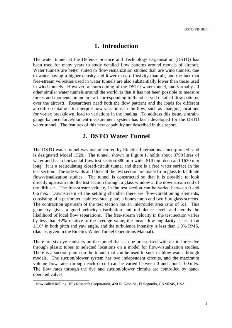
The DSTO water tunnel was manufactured by Eidetics International Incorporated1 and is designated Model 1520. The tunnel, shown in Figure 1, holds about 3790 litres of water and has a horizontal-flow test section 380 mm wide, 510 mm deep and 1630 mm long. It is a recirculating closed-circuit tunnel and there is a free water surface in the test section. The side walls and floor of the test section are made from glass to facilitate flow-visualization studies. The tunnel is constructed so that it is possible to look directly upstream into the test section through a glass window at the downstream end of the diffuser. The free-stream velocity in the test section can be varied between 0 and 0.6 m/s. Downstream of the settling chamber there are flow-conditioning elements, consisting of a perforated stainless-steel plate, a honeycomb and two fibreglass screens. The contraction upstream of the test section has an inlet/outlet area ratio of 6:1. This geometry gives a good velocity distribution and turbulence level, and avoids the likelihood of local flow separations. The free-stream velocity in the test section varies by less than ±2% relative to the average value, the mean flow angularity is less than ±1.0° in both pitch and yaw angle, and the turbulence intensity is less than 1.0% RMS, (data as given in the Eidetics Water Tunnel Operations Manual). There are six dye canisters on the tunnel that can be pressurised with air to force dye through plastic tubes to selected locations on a model for flow-visualization studies. There is a suction pump on the tunnel that can be used to suck or blow water through models. The suction/blower system has two independent circuits, and the maximum volume flow rates through each circuit can be varied between 0 and about 100 ml/s. The flow rates through the dye and suction/blower circuits are controlled by hand-operated valves. 1 Now called Rolling Hills Research Corporation, 420 N. Nash St., El Segundo, CA 90245, USA.
DSTO-TR-1835
2
Settling chamber
Pipe for water return
Screens
Contraction
C-strut
Diffuser
Test section380 x 510 mm
Model
Window
(a)
(b)
Figure 1. Eidetics Model 1520 water tunnel. (a) diagrammatic view of tunnel, (b) photograph of tunnel.
DSTO-TR-1835
3
Models are mounted on a C-strut so that the required centre of rotation of a model is at the centre of the imaginary circle formed by the strut, ensuring that all angular motion of the model is about this point. The model supporting system is attached to the top of the test section by a hinge, so that a model can be lowered into the test section, or removed from the test section, as required. When a model has been lowered, its centre of rotation is at the mid transverse position in the test section, 270 mm from the floor and 965 mm downstream of the start of the test section.
3. Strain-Gauge Balance
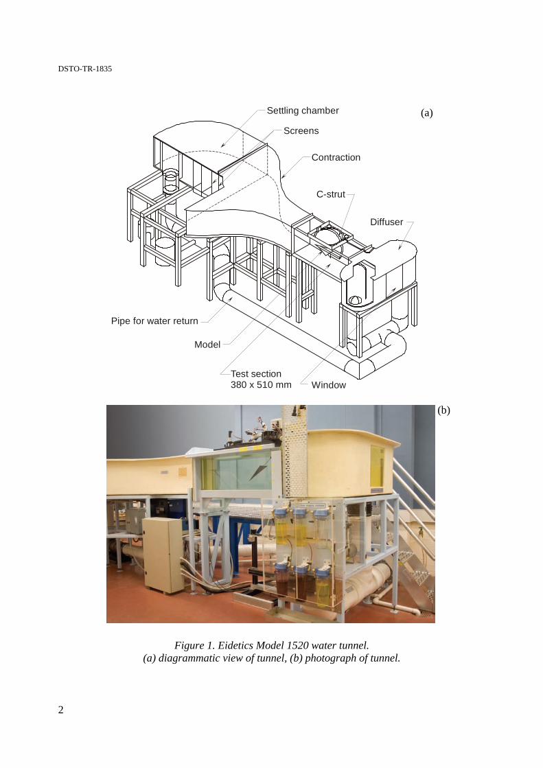
A sensitive two-component strain-gauge balance, shown in Figure 2, has been designed, manufactured and tested to measure normal forces and pitching moments. The balance is an integral unit, machined out of stainless steel rod, with a specification AISI 630 Condition H480. The dimensions of the flexure member and the likely deflection of the balance under load were determined using finite-element analysis. A model is bolted onto the balance at its tapered end. The flow-induced loads on aircraft in the water tunnel are small by conventional standards, and the balance has been designed to measure normal forces and pitching moments within the ranges ±2.5 N and ±0.02 N.m respectively. The loads were determined by scaling force and moment data measured on full-size combat aircraft during manoeuvres. For comparison, the balances used in the DSTO low-speed wind tunnel (LSWT) are typically designed to measure normal forces and pitching moments within the ranges ±3500 N and ±300 N.m respectively. The test section of the LSWT has cross-sectional dimensions of 2.74 m (width) by 2.13 m (height) and the maximum velocity obtainable in the test section is about 100 m/s. There is a factor of 1400 for normal forces and 15000 for pitching moments between the loads for the balances for the two tunnels.
All dimensions in mm22.5 25
285.8
19.310
Figure 2. Two-component balance, showing the main dimensions.
DSTO-TR-1835
4
Y
X
n
Zl
m
R R2dR 2a
2c2b RRR R
5V
Output
+ -
Normal-force bridge Pitching-moment bridge
Output
5V
1b 1c
1aR 1d
-+Input Input
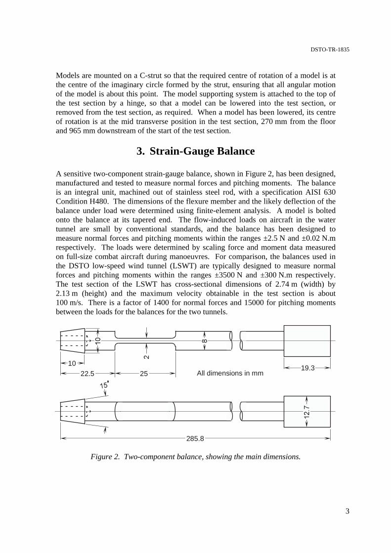
Figure 3. Two-component balance, showing the position of the gauges for the normal-
force and pitching-moment circuits, together with the corresponding bridges. Due to the small loads, semi-conductor strain gauges have been used, having a resist-ance of 1000 Ω, a gauge factor of 145, and dimensions of 1.27 mm by 0.15 mm (active area, length by width). The gauges were manufactured by PSI-TRONIX Incorporated2 and the model number of the gauges is P01-05-1000. The balance contains four gauges on each of the two sides of the flexure member, as shown in Figure 3. Gauges 1b, 1c, 2d and 2b, which are obscured, are on the opposite side of the flexure member and are directly underneath gauges 1a, 1d, 2a and 2c respectively. The eight gauges are connected together to form two Wheatstone bridges, as shown. The gauges have been positioned on the flexure member and wired together so that the normal forces and pitching moments measured by the balance are not affected by other load components, such as transverse forces and rolling moments. 2 PSI-TRONIX Incorporated, 3950 South “K” Street, Tulare, CA, 93274, USA.
DSTO-TR-1835
5
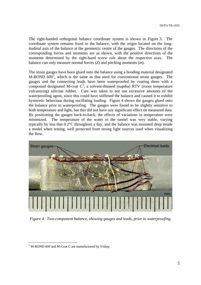
The right-handed orthogonal balance coordinate system is shown in Figure 3. The coordinate system remains fixed to the balance, with the origin located on the long-itudinal axis of the balance at the geometric centre of the gauges. The directions of the corresponding forces and moments are as shown, with the positive directions of the moments determined by the right-hand screw rule about the respective axes. The balance can only measure normal forces (Z) and pitching moments (m). The strain gauges have been glued onto the balance using a bonding material designated M-BOND 6003, which is the same as that used for conventional strain gauges. The gauges and the connecting leads have been waterproofed by coating them with a compound designated M-coat C3, a solvent-thinned (naptha) RTV (room temperature vulcanizing) silicone rubber. Care was taken to not use excessive amounts of the waterproofing agent, since this could have stiffened the balance and caused it to exhibit hysteretic behaviour during oscillating loading. Figure 4 shows the gauges glued onto the balance prior to waterproofing. The gauges were found to be slightly sensitive to both temperature and light, but this did not have any significant effect on measured data. By positioning the gauges back-to-back, the effects of variations in temperature were minimized. The temperature of the water in the tunnel was very stable, varying typically by less that 0.2°C throughout a day, and the balance was mounted deep inside a model when testing, well protected from strong light sources used when visualizing the flow.
Figure 4. Two-component balance, showing gauges and leads, prior to waterproofing.
3 M-BOND 600 and M-Coat C are manufactured by Vishay.
DSTO-TR-1835
6
4. Signal-Conditioning System
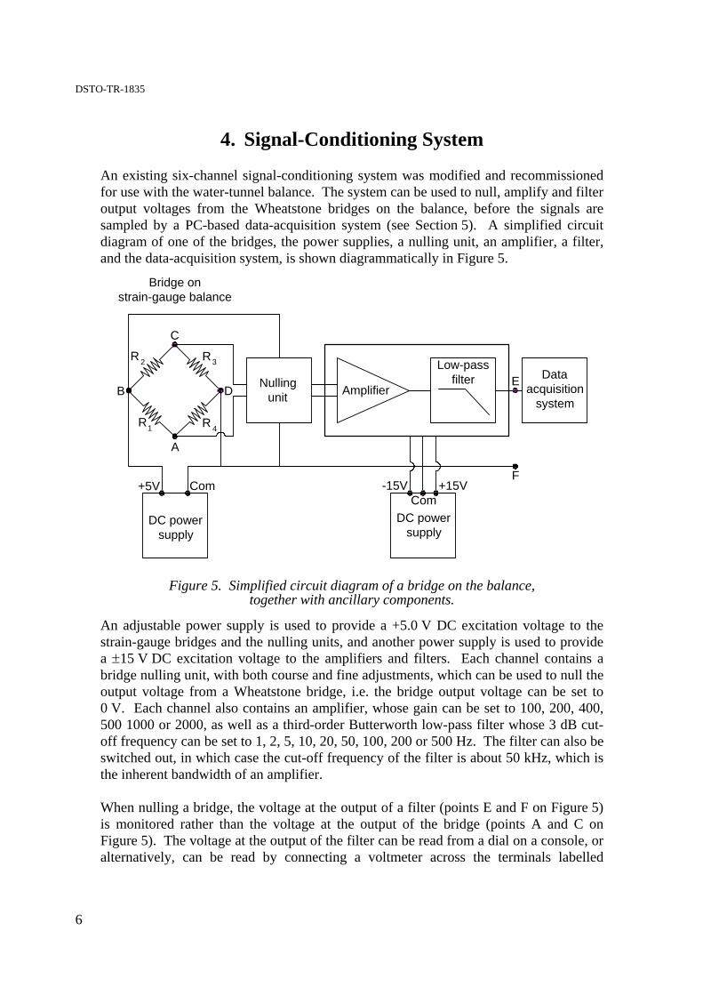
An existing six-channel signal-conditioning system was modified and recommissioned for use with the water-tunnel balance. The system can be used to null, amplify and filter output voltages from the Wheatstone bridges on the balance, before the signals are sampled by a PC-based data-acquisition system (see Section 5). A simplified circuit diagram of one of the bridges, the power supplies, a nulling unit, an amplifier, a filter, and the data-acquisition system, is shown diagrammatically in Figure 5.
EDB
C
A
+5V Com -15V +15VCom
Amplifier
Low-passfilter Data
acquisition system
Nullingunit
DC powersupply
DC powersupply
F
2R 3R
4R1R
Bridge onstrain-gauge balance
Figure 5. Simplified circuit diagram of a bridge on the balance,
together with ancillary components. An adjustable power supply is used to provide a +5.0 V DC excitation voltage to the strain-gauge bridges and the nulling units, and another power supply is used to provide a ±15 V DC excitation voltage to the amplifiers and filters. Each channel contains a bridge nulling unit, with both course and fine adjustments, which can be used to null the output voltage from a Wheatstone bridge, i.e. the bridge output voltage can be set to 0 V. Each channel also contains an amplifier, whose gain can be set to 100, 200, 400, 500 1000 or 2000, as well as a third-order Butterworth low-pass filter whose 3 dB cut-off frequency can be set to 1, 2, 5, 10, 20, 50, 100, 200 or 500 Hz. The filter can also be switched out, in which case the cut-off frequency of the filter is about 50 kHz, which is the inherent bandwidth of an amplifier. When nulling a bridge, the voltage at the output of a filter (points E and F on Figure 5) is monitored rather than the voltage at the output of the bridge (points A and C on Figure 5). The voltage at the output of the filter can be read from a dial on a console, or alternatively, can be read by connecting a voltmeter across the terminals labelled
DSTO-TR-1835
7
OUTPUT on the console. A sampling program, named ZERO BALANCE, based on LabVIEW4 software, has also been developed so that the voltage can be read on a monitor using a graphical user interface.
5. PC and Data-Acquisition Card
The PC used has a WindowsTM XP Professional operating system, a 3.2 GHz central processing unit, a 220 GB hard disk drive and 1 GB of RAM. The data-acquisition card interfaced with the PC was manufactured by National InstrumentsTM and the product code is NI 6013. The card features 16 channels (8 differential) of 16-bit analogue input, a 68 pin connector and 8 lines of digital input/output. Analogue input voltages varying between –5 V and +5 V can be sampled. For the 16-bit card, the resolution of the sampled voltages is 10.0/216, i.e. 10.0/65536 = 0.000153 V/LSB = 0.153 mV/LSB (LSB denotes least significant bit). When carrying out tests, it was not possible to “see” the actual loads measured by the balance. Loads had to be determined from the measured voltages, using calibration relationships, after the tests had been completed.
6. Calibration of the Strain-Gauge Balance
6.1 Balance Calibration Equations
The format of the calibration relationships depends upon which particular balance calibration model or set of equations is chosen to represent the data. There are a number of different sets of equations that can be used, but the one currently used at DSTO for the wind-tunnel balances assumes that balance output voltages are functions of the calibration coefficients and the applied loads (see Lam 1989, Leung & Link 1999, Blandford 2004). This model will also be used for the water-tunnel balance. For a perfect balance, the output voltage from say the normal-force channel is only affected by the normal force applied to the balance, and similarly for other channels. However, in practice, balances are not ideal and there may be interactions between the different channels, so that the output voltage from each channel generally depends on all of the load components applied to the balance. For the two-component balance, the calibration is always described by two different equations, but the number of terms in each equation can vary depending on whether the equations are first-order, second-order, third-order and so on. Both first-order and second-order calibrations were carried out and the equations and the calibration
4 LabVIEWTM, a graphical programming language, is a product of National Instruments.
DSTO-TR-1835
8
coefficients are given in this report, but loads on a delta-wing model were computed using first-order equations (see Section 8). The first-order equations are given by 22,111,11 HCHCR += (1) and 22,211,22 HCHCR += (2) R1 and R2 are voltage ratios for the normal-force and pitching-moment channels respectively, i.e. the output voltages from the channels divided by the respective input voltages to the channels, H1 and H2 are the applied normal force and pitching moment respectively, and the C terms are calibration coefficients. The second-order equations are given by 2112,1
2222,1
2111,122,111,11 HHCHCHCHCHCR ++++= (3)
and 2112,2
2222,2
2111,222,211,22 HHCHCHCHCHCR ++++= (4)
The two first-order equations, expressed in matrix form, are given by
⎥⎦
⎤⎢⎣
⎡⎥⎦
⎤⎢⎣
⎡=⎥
⎦
⎤⎢⎣
⎡
2
1
2,21,2
2,11,1
2
1
HH
CCCC
RR
(5)
and similarly, the two second-order equations, expressed in matrix form, are given by
⎥⎥⎥⎥⎥⎥
⎦
⎤
⎢⎢⎢⎢⎢⎢
⎣
⎡
⎥⎦
⎤⎢⎣
⎡=⎥
⎦
⎤⎢⎣
⎡
21
22
21
2
1
12,222,211,22,21,2
12,122,111,12,11,1
2
1
HHHHHH
CCCCCCCCCC
RR
(6)
Equations 5 and 6 can be expressed in a simplified matrix form as follows: [ ] [ ] [ ]HCR = (7) 6.2 Acquisition of Calibration Data
The balance was calibrated manually using the experimental setup shown in Figure 6. The balance was clamped onto a vee-block using a stirrup clamp (not shown) so that its
DSTO-TR-1835
9
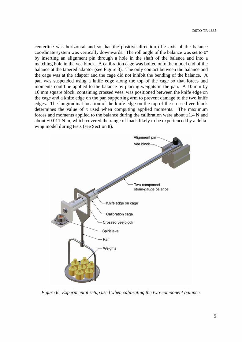
centerline was horizontal and so that the positive direction of z axis of the balance coordinate system was vertically downwards. The roll angle of the balance was set to 0º by inserting an alignment pin through a hole in the shaft of the balance and into a matching hole in the vee block. A calibration cage was bolted onto the model end of the balance at the tapered adaptor (see Figure 3). The only contact between the balance and the cage was at the adaptor and the cage did not inhibit the bending of the balance. A pan was suspended using a knife edge along the top of the cage so that forces and moments could be applied to the balance by placing weights in the pan. A 10 mm by 10 mm square block, containing crossed vees, was positioned between the knife edge on the cage and a knife edge on the pan supporting arm to prevent damage to the two knife edges. The longitudinal location of the knife edge on the top of the crossed vee block determines the value of x used when computing applied moments. The maximum forces and moments applied to the balance during the calibration were about ±1.4 N and about ±0.011 N.m, which covered the range of loads likely to be experienced by a delta-wing model during tests (see Section 8).
Figure 6. Experimental setup used when calibrating the two-component balance.
DSTO-TR-1835
10
For the current calibration, the gain of the amplifiers was set to 500 and the cut-off frequency of the low-pass filters was set to 1 Hz. Prior to commencing each loading sequence, when there were no weights in the pan, the output voltages from the two channels were nulled, i.e. the bridge output voltages were set close to 0.0 V. The method used to null the bridges is described in Section 4. Weights were progressively added to the pan, and then progressively removed, for the pan positioned at different x locations along the knife edge. The x locations used were -8.0, 0.0 and +8.0 mm, and for each of these locations the weights used were 0 to 140 to 0 g, in increments/decrements of 20 g. For each of the 15 loads used, the output voltages from the normal-force channel and from the pitching-moment channel were sampled 20 times at 0.1 s intervals and each set of 20 samples was then averaged to obtain mean values. The balance was rolled 180° and the above loading sequence was repeated for the same x locations, so that the loading was in the opposite direction. Altogether, 90 calibration points were taken for the normal-force channel and 90 corresponding points for the pitching-moment channel (15 loads for each of 2 directions at each of 3 x locations). A sampling program, named SCAN, based on LabVIEWTM, was developed to facilitate the calibration process. For each of the 90 pairs of calibration points, the user had to specify the number of samples, time between samples, output file name, applied load, excitation voltage, temperature, gain settings and filter settings. The program was then run and the output voltages from the different channels were displayed on the monitor in graphical form as they were being sampled. The voltages were written to a spreadsheet file along with other information specified by the user. Input conditions were updated for the next pair of calibration points and the procedure was repeated. Six individual data files were created for the complete calibration. 6.3 Plots of Voltage Ratios vs Loads
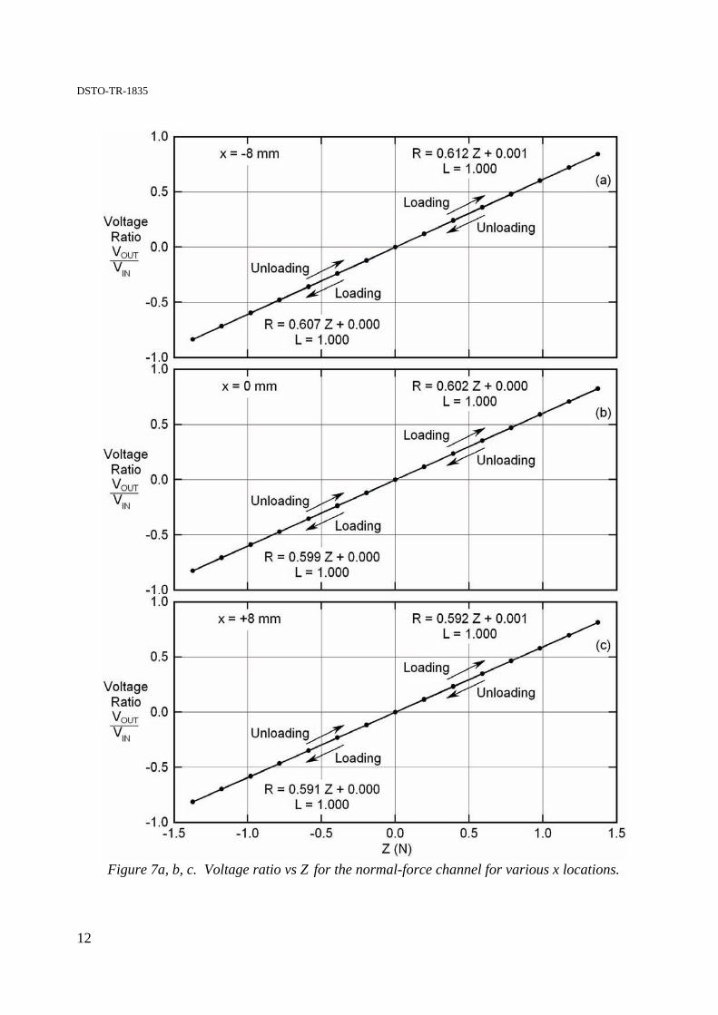
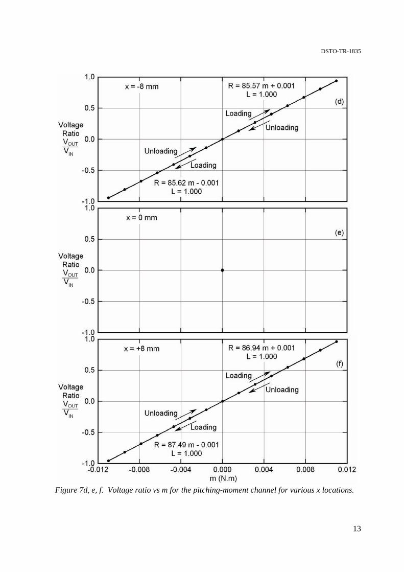
For the calibration data, plots of VOUT/VIN vs Z for the normal-force channel and plots of VOUT/VIN vs m for the pitching-moment channel are shown in Figure 7. Z is the applied normal force, m is the applied pitching moment, VOUT is the output voltage from a channel and VIN is the input voltage to the Wheatstone bridge for that channel (VIN is nominally 5.0 V). Each set of calibration points, corresponding to loading and unloading the balance at a given x location, occupies one quadrant on a plot. For Figures 7a and 7c, the pitching moments are different for each value of Z, and for Figures 7d and 7f, the normal forces are different for each value of m. Corresponding points for the loading and the unloading phases are almost coincident, with no discernable evidence of hysteretic behaviour. Figure 7e shows that for pure normal-force loading (for loads to ±140 g) at x = 0 mm, the output voltages from the pitching-moment channel are very small, i.e. there is very little cross coupling, and the 30 calibration points are superimposed. Where applicable, each set of experimental points has been curve fitted by a straight line using the method of least squares, and the
DSTO-TR-1835
11
equations for the straight lines are as shown (R ≡ VOUT/VIN). The values of the linear correlation coefficients, L, are also given. Each set of experimental points closely follow a straight line, as indicated by the values of L being close to 1.0. 6.4 Evaluation of Calibration Coefficients
The calibration coefficients were determined from the discrete applied loads and associated balance output/input voltages using the least-squares regression method proposed by Ramaswamy et al. (1987). Details of the procedure used are given in Appendix A. The first-order calibration coefficients are
⎥⎦
⎤⎢⎣
⎡++
=⎥⎦
⎤⎢⎣
⎡18.640E3-4.752E-01.139E1-6.006E
2,21,2
2,11,1
CCCC
(8)
and the second-order coefficients are
⎥⎦
⎤⎢⎣
⎡++++
=⎥⎦
⎤⎢⎣
⎡1-1.070E-12.087E-3-2.322E18.640E3-4.752E-
1-1.117E05.001E3-1.640E01.139E1-6.006E
12,222,211,22,21,2
12,122,111,12,11,1
CCCCCCCCCC
(9)
6.5 Checking Accuracy of Calibration
When calibrating a balance, loads are applied to the balance and corresponding output/input voltage ratios are measured. To check the accuracy of the calibration, the reverse procedure is used, whereby the calibration equations are used to estimate loads corresponding to the voltage ratios measured during the calibration. For an ideal calibration, the applied and estimated loads should be the same, but in practice small discrepancies do occur. Normal forces and pitching moments were estimated for the measured voltage ratios by using equation 7. Since the loads (H terms) are not an explicit function of the calibration coefficients (C terms) and the voltage ratios (R terms), then the loads had to be estimated iteratively. Details of how to do this are given by Fairlie (1985) and Leung & Link (1999). However, provided that [C] is a non-singular square matrix, then [C]-1 (inverse of [C]) can be formed and equation 7 can be rearranged to give [ ] [ ] [ ]RCH 1−= (10) enabling the loads to be estimated directly. This equation can only apply to the first-order equations, and not to the second-order equations, since [C] is a square matrix for only the first-order equations.
DSTO-TR-1835
12
Figure 7a, b, c. Voltage ratio vs Z for the normal-force channel for various x locations.
DSTO-TR-1835
13
Figure 7d, e, f. Voltage ratio vs m for the pitching-moment channel for various x locations.
DSTO-TR-1835
14
A statistical indicator commonly used to assess the accuracy of the calibration is the standard error (see Lam 1989 and Leung & Link 1999). The parameter indicates the goodness of the fit of the calibration equation and the uncertainties in the coefficients determined by the least-squares method. The standard errors for the normal force and the pitching moments are given by the following respective expressions
[ ]
fN
HHse
−
−=∑=
N
1PP,1P,1
1
~ 2
(11)
[ ]
fN
HHse
−
−=∑=
N
1PP,2P,2
2
~ 2
(12)
where se1 is the standard error for the normal forces, P,1H is an applied normal force,
P,1~H is the corresponding normal force estimated using the calibration equation, N is the
total number of points used in the calibration for each channel (N = 90), P is an index of summation and f is the number of degrees of freedom in the calibration equations. (The number of degrees of freedom is equal to the number of calibration coefficients per component, i.e. f = 2 for the first-order calibration equations and f = 5 for the second-order equations). The corresponding terms for the pitching moments, i.e. se2, P,2H and
PH ,2~ , are similarly defined. The standard error given by equation 11 has units of
Newton and that given by equation 12 has units of Newton meter. To convert the standard errors to dimensionless parameters, they are divided by the appropriate maximum design load, either a force or a pitching moment. For the first-order calibration, the standard errors were found to be 0.1% for the normal-force channel and 0.1% for the pitching-moment channel. This suggests that loads measured by the water-tunnel balance immediately after the calibration are of acceptable accuracy. 6.6 Checking Stability of Calibration
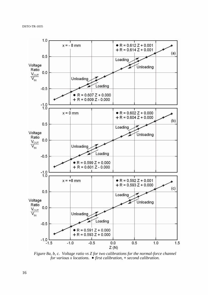
To check the stability of the calibration over time, the balance was recalibrated seven days after the initial calibration, using the same loading sequence, and the two calibrations were compared to see if there were any significant changes. Plots of VOUT/VIN vs Z for the two calibrations for the normal-force channel and plots of VOUT/VIN vs m for the two calibrations for the pitching-moment channel are shown in Figure 8. Each set of data points has been curve fitted by a straight line using the method of least squares, and the equations for the straight lines are as shown. Corresponding data from the two calibrations are almost coincident, showing that the calibration is stable over the time interval considered.
DSTO-TR-1835
15
A reverse calibration procedure was applied to both calibrations, whereby equation 10 was used to estimate loads from voltage ratios measured during the calibrations. Loads were estimated using (a) the voltage ratios from the first calibration combined with the calibration coefficients determined from the first calibration, and (b) the voltage ratios from the first calibration combined with the calibration coefficients determined from the second calibration. For the complete range of calibration points considered, it was found that the variation in estimated normal forces for cases (a) and (b) was always within the range ±0.8%, and the variation in estimated pitching moments for the two cases was always within the range ±0.3%. Thus, there is good agreement between the first and second calibrations, confirming the above finding that the calibration did not change significantly over the time interval considered.
7. Checking Waterproofing of Balance
Tests were undertaken to see whether the strain gauges and the electrical leads on the balance were affected by water. The balance was submerged in water for a period of 10 hours between the first and second calibrations (see Section 6.6), and while under water, the gauges on the balance were active, i.e. the two bridges on the balance were supplied with an excitation voltage of 5 V DC. The two calibrations agreed closely, as shown in Section 6.6, indicating that the waterproofing agent on the balance was effective.
8. Tests Using a Delta Wing
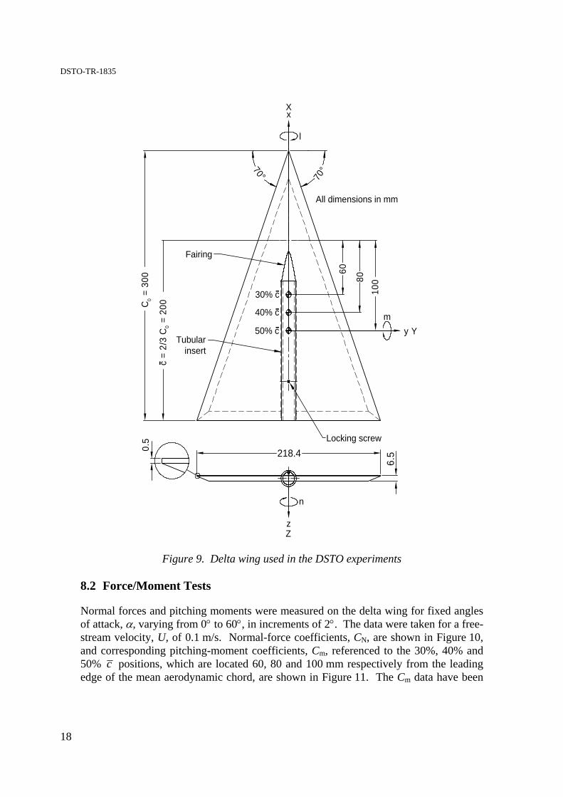
The strain-gauge balance was used to measure forces and moments on a 70º delta wing to see if the results agreed with those reported in the literature. A delta wing is an ideal test model to use when comparing data obtained in different wind and water tunnels. The reason for this is that the flow over a delta wing at an angle of attack is dominated by two large bound vortices that are formed by the rolling up of the flow as it separates along the two leading edges of the wing. The flow over such a wing in different facilities is consistent and well defined, and the way the associated normal forces and pitching-moments vary with angle of attack are well established. 8.1 Details of Delta Wing
The delta wing used in the tests is shown in Figure 9. The wing is made from clear Perspex. The leading edges of the wing are square to the leeward (suction) surface for the first 0.5 mm from that surface, and they are then bevelled at an angle of 30°. For a delta wing, the mean aerodynamic chord (mac) is 2/3 of the root chord, i.e. c = (2/3) C0 = 200.0 mm. The coordinate system (x, y, z) is as shown. A metal tubular insert is embedded in the wing along its centreline to allow it to be fitted onto a strain-gauge balance, and the insert is faired into the windward and leeward sides of the wing as shown. The two-component balance was positioned in the insert so that the origin of the balance coordinate system was located at the 50% mac position shown in Figure 9.
DSTO-TR-1835
16
Figure 8a, b, c. Voltage ratio vs Z for two calibrations for the normal-force channel
for various x locations. • first calibration, + second calibration.
DSTO-TR-1835
17
Figure 8d, e, f. Voltage ratio vs m for two calibrations for the pitching-moment channel for various x locations. • first calibration, + second calibration.
DSTO-TR-1835
18
--
8010
0
C =
300
218.4
6.5
70°70°
Fairing
Locking screw
0
0c
= 2/
3 C
= 2
00-
60
-
All dimensions in mm
Tubularinsert
0.5
Xx
l
y Ym
Zz
n
30% c
40% c
50% c
Figure 9. Delta wing used in the DSTO experiments 8.2 Force/Moment Tests
Normal forces and pitching moments were measured on the delta wing for fixed angles of attack, α, varying from 0° to 60°, in increments of 2°. The data were taken for a free-stream velocity, U, of 0.1 m/s. Normal-force coefficients, CN, are shown in Figure 10, and corresponding pitching-moment coefficients, Cm, referenced to the 30%, 40% and 50% c positions, which are located 60, 80 and 100 mm respectively from the leading edge of the mean aerodynamic chord, are shown in Figure 11. The Cm data have been
DSTO-TR-1835
19
computed relative to these three reference positions to facilitate comparing the data with that obtained by other researchers. CN and Cm were computed from balance output voltages using first-order calibration equations. Each experimental point shown in Figures 10 and 11 corresponds to 50 sets of gauge output voltages, sampled at 1 s intervals per set. Data were corrected for the effects of tunnel blockage using the corrections proposed by Cunningham & Bushlow (1990). The corrections were only made for values of α greater than those corresponding to maximum static values of CN (as was done by Cunningham & Bushlow). The corrections were required as a result of a significant expansion of the wing wake when the wing stalls. For the current tests, this value of α, denoted by αts, was 38°. Cunningham & Bushlow developed a semi-empirical relationship, based on the angle of attack of a model and its blockage, as follows. 2
mtWted)N(uncorrecd)N(correcte )sin1( α′−= ACCC (13) For α > 38°, CW, an empirical coefficient, is equal to 1.57, Amt is the ratio of the model projected cross-sectional area (as viewed in the free-stream direction) to the test section cross-sectional area, and α ′ is given by
⎟⎟⎠
⎞⎜⎜⎝
⎛−−
=′ts
ts
9090
αααα (14)
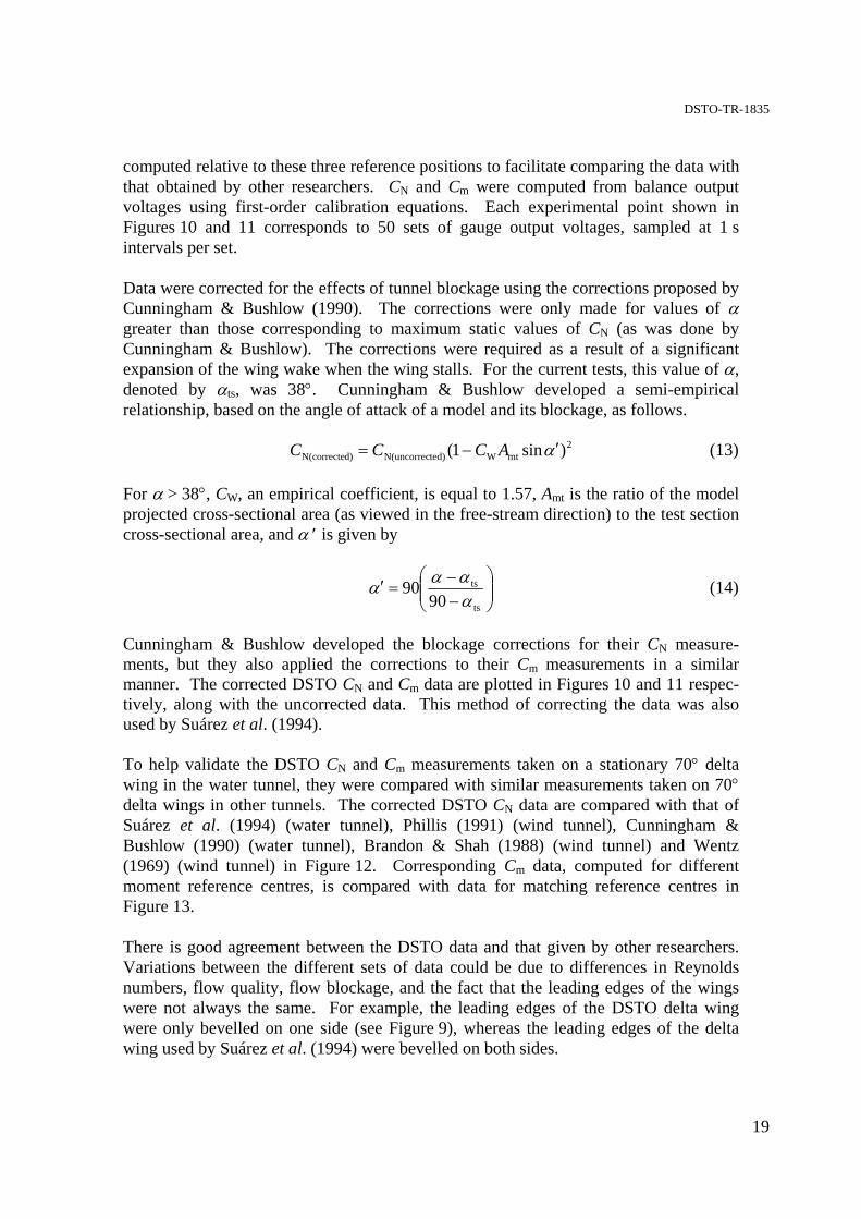
Cunningham & Bushlow developed the blockage corrections for their CN measure-ments, but they also applied the corrections to their Cm measurements in a similar manner. The corrected DSTO CN and Cm data are plotted in Figures 10 and 11 respec-tively, along with the uncorrected data. This method of correcting the data was also used by Suárez et al. (1994). To help validate the DSTO CN and Cm measurements taken on a stationary 70° delta wing in the water tunnel, they were compared with similar measurements taken on 70° delta wings in other tunnels. The corrected DSTO CN data are compared with that of Suárez et al. (1994) (water tunnel), Phillis (1991) (wind tunnel), Cunningham & Bushlow (1990) (water tunnel), Brandon & Shah (1988) (wind tunnel) and Wentz (1969) (wind tunnel) in Figure 12. Corresponding Cm data, computed for different moment reference centres, is compared with data for matching reference centres in Figure 13. There is good agreement between the DSTO data and that given by other researchers. Variations between the different sets of data could be due to differences in Reynolds numbers, flow quality, flow blockage, and the fact that the leading edges of the wings were not always the same. For example, the leading edges of the DSTO delta wing were only bevelled on one side (see Figure 9), whereas the leading edges of the delta wing used by Suárez et al. (1994) were bevelled on both sides.
DSTO-TR-1835
20
-0.5
0.0
0.5
1.0
1.5
2.0
2.5
0 10 20 30 40 50 60
NormalForce
CoefficientC
N
Angle of Attack α (deg)
Corrected dataUncorrected data
Figure 10. Normal-force coefficients for the DSTO delta wing.
-0.2
-0.1
0.0
0.1
0.2
0.3
0.4
0 10 20 30 40 50 60
PitchingMoment
CoefficientC
m
Angle of Attack α (deg)
Corrected dataUncorrected data
50% c
40% c
30% c
Figure 11. Pitching-moment coefficients for the DSTO delta wing.
DSTO-TR-1835
21
-0.5
0.0
0.5
1.0
1.5
2.0
2.5
0 10 20 30 40 50 60
NormalForce
CoefficientC
N
Angle of Attack α (deg)
Suarez et al. (1994)Data from current investigation
Phillis (1991)Cunningham & Bushlow (1990)Brandon & Shah (1988)Wentz (1969)
Figure 12. Normal-force coefficients for the DSTO delta wing compared with other data.
-0.2
-0.1
0.0
0.1
0.2
0.3
0.4
0 10 20 30 40 50 60
PitchingMoment
CoefficientC
m
Angle of Attack α (deg)
Suarez et al. (1994)Data from current investigation
Phillis (1991)Brandon & Shah (1988)Wentz (1969)
50% c
40% c
30% c
Figure 13. Pitching-moment coefficients for the DSTO delta wing compared with other data.
DSTO-TR-1835
22
9. Concluding Remarks
This report provides details of a strain-gauge-balance force/moment measurement system that was developed to measure flow-induced loads on models in the DSTO water tunnel. The loads are small by conventional standards and the balance was designed to measure normal forces and pitching moments within the ranges ±2.5 N and ±0.02 N.m respectively. Strain-gauge balances having such low load ranges have not been used previously within DSTO. For comparison, the balances used in the low-speed wind tunnel at DSTO regularly measure loads greater than 1000 times these values. To measure the small loads, it was necessary to use semi-conductor strain gauges on the balance. The calibration of the balance was found to be accurate to within ±0.1% and also stable, and the waterproofing of the balance was found to be effective. The new system was used to measure loads on a 70º delta wing for a range of static angles of attack. Measured normal-force and pitching-moment coefficients agreed well with wind- and water-tunnel data reported in the literature, showing that the new system gives good results, at least for a sharp-edged delta wing, where flow patterns are independent of Reynolds number. The ability to measure the small flow-induced loads on a model in the water tunnel increases the usefulness of the tunnel, and complements earlier work done at DSTO, in which the small flow-induced pressures on the surface of a model in the tunnel were measured (Erm 2000). The load-measurement system has recently been incorporated into a dynamic-testing system that enables loads to be measured on an aircraft model as it undergoes a defined dynamic manoeuvre (Erm 2006).
10. Acknowledgements
The author is grateful for the help given by the following two people. The project was substantial and could not have been completed without their significant input. Phil Ferrarotto
• For mounting the semi-conductor strain gauges onto the chassis
of the balance and for waterproofing the balance. Michael Konak
• For recommissioning an existing strain-gauge-balance signal-
conditioning system and for writing software for a data-acquisition system.
DSTO-TR-1835
23
11. References Blandford, A. 2004 Calibration of the sensitivity matrix of the Collins strain gauge
Brandon, J. M. & Shah, G. H. 1988 Effect of large amplitude pitching moments on the unsteady aerodynamic characteristics of flat-plate wings. Paper 88-4331-CP, AIAA Atmospheric Flight Mechanics Conference, Minneapolis, MN, USA, Aug 15-17
Cunningham, A. M. Jr. & Bushlow, T. 1990 Steady and unsteady force testing of fighter aircraft models in a water tunnel. Paper 90-2815-CP, AIAA 8th Applied Aerodynamics Conference, Portland, OR, USA, Aug 20-22.
Erm, L. P. 2000 An investigation into the feasibility of measuring flow-induced pressures on the surface of a model in the AMRL water tunnel. DSTO-TN-0323, Aeronautical and Maritime Research Laboratory, Defence Science and Technology Organisation, Melbourne, Australia.
Erm, L. P. 2006 Development and use of a dynamic-testing capability for the DSTO water tunnel. DSTO-TR-1836, Defence Science and Technology Organisation, Melbourne, Australia.
Fairlie, B. D. 1985 Algorithms for the reduction of wind-tunnel data derived from strain gauge force balances. Aerodynamic Report 164, Aeronautical Research Laboratories, Defence Science and Technology Organisation, Melbourne, Australia.
Lam, S. S. W. 1989 A FORTRAN program for the calculation of the calibration coefficients of a six-component strain gauge balance. Flight Mechanics Technical Memorandum 410, Aeronautical Research Laboratory, Defence Science and Technology Organisation, Melbourne, Australia.
Leung, S. Y. F. & Link, Y. Y. 1999 Comparison and analysis of strain gauge balance calibration matrix mathematical models. DSTO-TR-0857, Aeronautical and Maritime Research Laboratory, Defence Science and Technology Organisation, Melbourne, Australia.
Phillis, D. L. 1991 Force and pressure measurements over a 70º delta wing at high angles of attack and sideslip. Masters Thesis, Aeronautical Engineering Department, The Wichita State University, USA.
Ramaswamy, M. A., Srinivas, T. & Holla, V. S. 1987 A simple method for wind tunnel balance calibration including non-linear interaction terms. Proceedings of the ICIASF '87 RECORD.
Suárez, C. J., Malcolm, G. N., Kramer, B. R., Smith, B. C. & Ayers, B. F. 1994 Development of a multicomponent force and moment balance for water tunnel applications, Volumes I and II. NASA Contractor Report 4642.
Wentz, W. H. Jr. 1969 Wind tunnel investigations of vortex breakdown on slender sharp-edged wings. PhD Dissertation, University of Kansas, Lawrence, KS, USA.
DSTO-TR-1835
24
DSTO-TR-1835
25
Appendix A: Evaluation of Calibration Coefficients
In Section 6.1, it was indicated that the first-order calibration relationships for the two-component balance were 22,111,11 HCHCR += (A1) and 22,211,22 HCHCR += (A2) and the corresponding second-order calibration relationships were 2112,1
2222,1
2111,122,111,11 HHCHCHCHCHCR ++++= (A3)
and 2112,2
2222,2
2111,222,211,22 HHCHCHCHCHCR ++++= (A4)
R1 and R2 are voltage ratios, viz. the output voltages from the normal-force and pitching-moment channels divided by the input voltages to those channels respectively, H1 and H2 are the applied normal force and pitching moment respectively, and the C terms are calibration coefficients. The coefficients appearing in these equations can be determined from the discrete applied loads and associated voltage ratios using a least-squares regression model. Various types of regression methods have been reported in the literature, but the method used when calibrating the wind-tunnel balances in Air Vehicles Division is that developed by Ramaswamy et al. (1987). This method was also used when calibrating the water-tunnel balance. Lam (1989) gives mathematical details of the method, and only an outline of the method will be given here –also see Leung & Link (1999) and Blandford (2004). The method will only be described for the second-order calibration equations (equations A3 and A4), but the same principles apply for equations of lower or higher orders. For this method, the calibration coefficients are established when the sum of the squares of the differences between the measured strain-gauge output voltage ratios and those obtained from a calibration equation are a minimum. That is,
[ ]∑=
−++++=N
1PP,1P,2P,112,1
2P,222,1
2P,111,1P,22,1P,11,11
2RHHCHCHCHCHCe (A5)
and
[ ]∑=
−++++=N
1PP,2P,2P,112,2
2P,222,2
2P,111,2P,22,2P,11,22
2RHHCHCHCHCHCe (A6)
DSTO-TR-1835
26
are both a minimum, where e1 and e2 are sums of squares of residuals for the normal-force and pitching-moment components respectively, P is an index of summation and N is the number of calibration points for each channel (N = 90 –see Section 6.2). The procedure involves partial differentiating e1 with respect to each of its coefficients and equating the resultant expressions to zero, and likewise for e2. This results in a set of 5 non-linear simultaneous equations for each of the two components as follows5: [ ] 0112112,1
2222,1
2111,122,111,1 =−++++∑ HRHHCHCHCHCHC
[ ] 0212112,1
2222,1
2111,122,111,1 =−++++∑ HRHHCHCHCHCHC
[ ] 02
112112,12222,1
2111,122,111,1 =−++++∑ HRHHCHCHCHCHC (A7)
[ ] 02
212112,12222,1
2111,122,111,1 =−++++∑ HRHHCHCHCHCHC
[ ] 02112112,1
2222,1
2111,122,111,1 =−++++∑ HHRHHCHCHCHCHC
and [ ] 0122112,2
2222,2
2111,222,211,2 =−++++∑ HRHHCHCHCHCHC
[ ] 0222112,2
2222,2
2111,222,211,2 =−++++∑ HRHHCHCHCHCHC
[ ] 02
122112,22222,2
2111,222,211,2 =−++++∑ HRHHCHCHCHCHC (A8)
[ ] 02
222112,22222,2
2111,222,211,2 =−++++∑ HRHHCHCHCHCHC
[ ] 02122112,2
2222,2
2111,222,211,2 =−++++∑ HHRHHCHCHCHCHC
Equations A7 and A8 can be combined and put into matrix notation as follows: [ ] [ ] [ ]ACE =T (A9) [C]T is the transpose of the matrix of calibration coefficients and is given by 5 For clarity, the subscript P on R and H is omitted in the remainder of this report. Whenever the summation symbol is used, it is to understood that the sum is to be taken over the range P = 1 to N.
The 25 elements comprising [E] and the 10 elements comprising [A] can each be determined from the known applied calibration loads and the corresponding measured voltage ratios, so that the 10 elements in [C]T can be determined by making use of equation A9. It is not possible to determine [C]T directly from this equation, and the equation must be rearranged to obtain an explicit expression for [C]T. Provided [E] is a non-singular square matrix, then [E]-1 (inverse of [E]) can be formed and equation A9 can be rearranged as follows: [ ] [ ] [ ]AEC 1T −= (A13) Once [C]T is known, [C] can be determined by simply transposing [C]T (equation A10) to give
[ ] ⎥⎦
⎤⎢⎣
⎡=
12,222,211,22,21,2
12,122,111,12,11,1
CCCCCCCCCC
C (A14)
DISTRIBUTION LIST
Development of a Two-Component Strain-Gauge-Balance Load-Measurement System for the DSTO Water Tunnel
Lincoln P. Erm
AUSTRALIA
Defence Organisation No. of Copies S&T Program
Chief Defence Scientist 1 Deputy Chief Defence Scientist Policy 1 AS Science Corporate Management 1 Director General Science Policy Development 1 Counsellor Defence Science, London Doc Data Sheet Counsellor Defence Science, Washington Doc Data Sheet Scientific Adviser to MRDC, Thailand Doc Data Sheet Scientific Adviser Joint 1 Navy Scientific Adviser Doc Data Sheet & Dist
List Scientific Adviser – Army Doc Data Sheet & Dist
List Air Force Scientific Adviser 1 Scientific Adviser to the DMO 1
Deputy Chief Defence Scientist Platform and Human Systems
Doc Data Sht & Exec Summary
Chief of Air Vehicles Division: D. Wyllie Doc Data Sht & Dist List
Research Leader Flight Systems: D. Graham Head Flight Mechanics: J. Drobik
1 Printed 1 Printed
Head Experimental Aerodynamics, Vibration and Aeroelasticity: N. Matheson Head Air Vehicle Systems Analysis: S. Henbest
1 Printed 1 Printed
L. Erm 9 Printed V. Baskaran A. Blandford G. Brian J. Clayton K. Desmond P. Ferrarotto R. Geddes
M. Giacobello A. Gonzalez S. Hill O. Holland P. Jacquemin M. Konak S. Lam
O. Levinski P. Manovski D. Newman P. O’Connor D. Sherman B. Woodyatt
20 Printed
DSTO Library and Archives
Library Fishermans Bend Doc Data Sheet Library Edinburgh 1 printed
Defence Archives 1 printed
Capability Development Executive
Director General Maritime Development Doc Data Sheet Director General Capability and Plans Doc Data Sheet Assistant Secretary Investment Analysis Doc Data Sheet Director Capability Plans and Programming Doc Data Sheet
Chief Information Officer Group
Head Information Capability Management Division Doc Data Sheet Director General Australian Defence Simulation Office Doc Data Sheet AS Information Strategy and Futures Doc Data Sheet Director General Information Services Doc Data Sheet
Strategy Executive
Assistant Secretary Strategic Planning Doc Data Sheet Assistant Secretary International and Domestic Security Policy Doc Data Sheet
Navy
Maritime Operational Analysis Centre, Building 89/90 Garden Island Sydney NSW Deputy Director (Operations) Deputy Director (Analysis)
Doc Data Sht & Dist List
Director General Navy Capability, Performance and Plans, Navy Headquarters
Doc Data Sheet
Director General Navy Strategic Policy and Futures, Navy Headquarters
Doc Data Sheet
Air Force SO (Science) - Headquarters Air Combat Group, RAAF Base, Williamtown NSW 2314
Doc Data Sht & Exec Summary
Staff Officer Science Surveillance and Response Group Doc Data Sht & Exec Summary
Army ABCA National Standardisation Officer Land Warfare Development Sector, Puckapunyal
Doc Data Sheet
J86 (TCS GROUP), DJFHQ Doc Data Sheet SO (Science) - Land Headquarters (LHQ), Victoria Barracks NSW Doc Data Sht & Exec
Summary SO (Science) - Special Operations Command (SOCOMD), R5-SB-15, Russell Offices Canberra
Doc Data Sht & Exec Summary
SO (Science), Deployable Joint Force Headquarters (DJFHQ) (L), Enoggera QLD
Doc Data Sheet
Joint Operations Command Director General Joint Operations Doc Data Sheet Chief of Staff Headquarters Joint Operations Command Doc Data Sheet Commandant ADF Warfare Centre Doc Data Sheet Director General Strategic Logistics Doc Data Sheet
Intelligence and Security Group AS Concepts, Capability and Resources 1
DGSTA , Defence Intelligence Organisation 1 Manager, Information Centre, Defence Intelligence Organisation 1 Director Advanced Capabilities Doc Data Sheet
Defence Materiel Organisation Deputy CEO Doc Data Sheet Head Aerospace Systems Division Doc Data Sheet Head Maritime Systems Division Doc Data Sheet Program Manager Air Warfare Destroyer Doc Data Sheet Guided Weapon & Explosive Ordnance Branch (GWEO) Doc Data Sheet CDR Joint Logistics Command Doc Data Sheet
OTHER ORGANISATIONS National Library of Australia 1 NASA (Canberra) 1
UNIVERSITIES AND COLLEGES
Australian Defence Force Academy Library Head of Aerospace and Mechanical Engineering
1 1
Monash University: Hargrave Library,
Doc Data Sheet
Professor J. Soria, 1 Printed University of Adelaide: Professor R. M. Kelso 1 Printed University of Melbourne: Engineering Library Emeritus Professor P. N. Joubert Professor M. S. Chong
1 Printed 1 Printed 1 Printed
OUTSIDE AUSTRALIA
ORGANISATIONS
Air force Research Laboratory Dr. M. Ol
1 Printed
Rolling Hills Research Corporation: Dr B. R. Kramer Dr M. F. Kerho
1 Printed 1 Printed
UNIVERSITIES AND COLLEGES Princeton University: Professor A. J. Smits University of Minnesota: Professor I. Marusic
1 Printed 1 Printed
INTERNATIONAL DEFENCE INFORMATION CENTRES
US Defense Technical Information Center 1 UK Dstl Knowledge Services 1 Canada Defence Research Directorate R&D Knowledge & Information Management (DRDKIM)
1
NZ Defence Information Centre 1
ABSTRACTING AND INFORMATION ORGANISATIONS Library, Chemical Abstracts Reference Service 1
Engineering Societies Library, US 1 Materials Information, Cambridge Scientific Abstracts, US 1 Documents Librarian, The Center for Research Libraries, US 1
INFORMATION EXCHANGE AGREEMENT PARTNERS
National Aerospace Laboratory, Japan 1 National Aerospace Laboratory, Netherlands 1 SPARES Total number of copies: 74 Printed: 49 PDF: 25
4 Printed
Page classification: UNCLASSIFIED
DEFENCE SCIENCE AND TECHNOLOGY ORGANISATION
DOCUMENT CONTROL DATA 1. PRIVACY MARKING/CAVEAT (OF DOCUMENT)
2. TITLE Development of a Two-Component Strain-Gauge-Balance Load-Measurement System for the DSTO Water Tunnel
3. SECURITY CLASSIFICATION (FOR UNCLASSIFIED REPORTS THAT ARE LIMITED RELEASE USE (L) NEXT TO DOCUMENT CLASSIFICATION) Document (U) Title (U) Abstract (U)
4. AUTHOR(S) Lincoln P. Erm
5. CORPORATE AUTHOR Defence Science and Technology Organisation 506 Lorimer St Fishermans Bend Victoria 3207 Australia
6a. DSTO NUMBER DSTO-TR-1835
6b. AR NUMBER AR-013-598
6c. TYPE OF REPORT Technical Report
7. DOCUMENT DATE March 2006
8. FILE NUMBER 2006/1004080/1
9. TASK NUMBER 04/182
10. TASK SPONSOR DSTO
11. NO. OF PAGES 26
12. NO. OF REFERENCES 12
13. URL on the World Wide Web http://www.dsto.defence.gov.au/corporate/reports/ DSTO-TR-1835.pdf
14. RELEASE AUTHORITY Chief, Air Vehicles Division
15. SECONDARY RELEASE STATEMENT OF THIS DOCUMENT
Approved for public release OVERSEAS ENQUIRIES OUTSIDE STATED LIMITATIONS SHOULD BE REFERRED THROUGH DOCUMENT EXCHANGE, PO BOX 1500, EDINBURGH, SA 5111 16. DELIBERATE ANNOUNCEMENT No Limitations 17. CITATION IN OTHER DOCUMENTS Yes 18. DEFTEST DESCRIPTORS Water tunnel tests, Strain gauges, Load tests, Aircraft models
This report provides details of a two-component strain-gauge balance and ancillary equipment that has been developed to measure flow-induced loads on models in the DSTO water tunnel. The loads are very small and the balance was designed to measure normal forces and pitching moments within the ranges ±2.5 N and ±0.02 N.m respectively. Due to the small loads, it was necessary to use semi-conductor strain gauges on the balance. Balances having such low load ranges have not previously been used within DSTO. The balance was used to measure forces and moments on a delta wing in the water tunnel for a range of fixed angles of attack. The measured loads showed good agreement with wind- and water-tunnel data reported in the literature, showing that the new load-measurement system gives good results.