Development of an Advanced Approach for Next-Generation ... of an Advanced Approach for Next... ·...

Advanced Resources InternationalAdvanced Resources International

Development of an Advanced Approach for Next-Generation Integrated Reservoir Characterization

Final Report

Period of Performance: October 1, 2001 – December 31, 2004 Authored By: Scott R. Reeves Advanced Resources International, Inc. Performed By: Advanced Resources International, Inc. 9801 Westheimer, Suite 805 Houston, Texas 77042

U.S. Department of Energy Award Number DE-FC26-01BC15357 April, 2005

i

Disclaimers

U.S. Department Of Energy Disclaimer This report was prepared as an account of work sponsored by an agency of the United States Government. Neither the United States Government nor any agency thereof, nor any of their employees, makes any warranty, express or implied, or assumes any legal liability or responsibility for the accuracy, completeness, or usefulness of any information, apparatus, product, or process disclosed, or represents that its use would not infringe privately owned rights. Reference herein to any specific commercial product, process, or service by trade name, trademark, manufacturer, or otherwise does not necessarily constitute or imply its endorsement, recommendation, or favoring by the United States Government or any agency thereof. The views and opinions of authors expressed herein do not necessarily state or reflect those of the United States Government or any agency thereof.

Advanced Resources International Disclaimer The material in this Report is intended for general information only. Any use of this material in relation to any specific application should be based on independent examination and verification of its unrestricted applicability for such use and on a determination of suitability for the application by professionally qualified personnel. No license under any Advanced Resources International, Inc., patents or other proprietary interest is implied by the publication of this Report. Those making use of or relying upon the material assume all risks and liability arising from such use or reliance.

ii

Abstract

Accurate, high-resolution, three-dimensional (3D) reservoir characterization can provide substantial benefits for effective oilfield management. By doing so, the predictive reliability of reservoir flow models, which are routinely used as the basis for investment decisions involving hundreds of millions of dollars and designed to recover millions of barrels of oil, can be significantly improved. Even a small improvement in incremental recovery for high-value assets can result in important contributions to bottom-line profitability.

Today’s standard practice for developing a 3D reservoir description is to use seismic

inversion techniques. These techniques make use of geostatistics and other stochastic methods to solve the inverse problem, i.e., to iteratively construct a likely geologic model and then upscale and compare its acoustic response to that actually observed in the field. This method has several inherent flaws, such as:

• The resulting models are highly non-unique; multiple equiprobable realizations are produced, meaning

• The results define a distribution of possible outcomes; the best they can do is quantify the uncertainty inherent in the modeling process, and

• Each realization must be run through a flow simulator and history matched to assess it’s appropriateness, and therefore

• The method is labor intensive and requires significant time to complete a field study; thus it is applied to only a small percentage of oil and gas producing assets.

A new approach to achieve this objective was first examined in a Department of Energy

(DOE) study performed by Advanced Resources International (ARI) in 2000/2001. The goal of that study was to evaluate whether robust relationships between data at vastly different scales of measurement could be established using virtual intelligence (VI) methods. The proposed workflow required that three specific relationships be established through use of artificial neural networks (ANN’s): core-to-log, log-to-crosswell seismic, and crosswell-to-surface seismic. One of the key attributes of the approach, which should result in the creation of high resolution reservoir characterization with greater accuracy and with less uncertainty than today’s methods, is the inclusion of borehole seismic (such as crosswell and/or vertical seismic profiling – VSP) in the data collection scheme. Borehole seismic fills a critical gap in the resolution spectrum of reservoir measurements between the well log and surface seismic scales, thus establishing important constraints on characterization outcomes.

The results of that initial study showed that it is, in fact, feasible to establish the three

critical relationships required, and that use of data at different scales of measurement to create high-resolution reservoir characterization is possible. Based on the results of this feasibility study, in September 2001, the DOE, again through ARI, launched a subsequent two-year government-industry R&D project to further develop and demonstrate the technology.

The goals of this project were to:

iii

Make improvements to the initial methodology by incorporating additional VI technologies (such as clustering), using core measurements in place of magnetic resonance image (MRI) logs, and streamlining the workflow, among others.

Demonstrate the approach in an integrated manner at a single field site, and validate it via

reservoir modeling or other statistical methods. Based on the results from the project, the following conclusions have been drawn:

• A reasonable reservoir characterization model was established for the McElroy field using clustering methods. The model provided results that appear consistent with known conditions at the field, and identified potential areas of poor reservoir quality to be avoided for future development. The clustering approach has the advantage over ANN methods in that the entire process can be performed with a single, integrated model as opposed to multiple, sequential models.

• Experimentation with and without cross-well data suggested that, in this case, cross-well

data actually harmed model performance. It is believed that the cross-well data was of poor quality, which may have introduced error into the process, creating this result.

• The process appeared to provide some, but not a significant level of, vertical resolution

enhancement to the surface seismic data. Again, the failure of the cross-well data to enhance the results may have contributed to this outcome.

• The engineering model to relate well logs to core data was very successful, even in this

complex reservoir environment. This procedure can be used in other environments to provide porosity and permeability estimates at well locations with log data. The clustering of well logs did not appreciably improve the process.

iv

Executive Summary

Accurate, high-resolution, three-dimensional (3D) reservoir characterization can provide substantial benefits for effective oilfield management. By doing so, the predictive reliability of reservoir flow models, which are routinely used as the basis for investment decisions involving hundreds of millions of dollars and designed to recover millions of barrels of oil, can be significantly improved. Even a small improvement in incremental recovery for high-value assets can result in important contributions to bottom-line profitability.








(DOE) study performed by Advanced Resources International (ARI) in 2000/2001. The goal of that study was to evaluate whether robust relationships between data at vastly different scales of measurement could be established using virtual intelligence (VI) methods. The proposed workflow required that three specific relationships be established through use of artificial neural networks (ANN’s): core-to-log, log-to-crosswell seismic, and crosswell-to-surface seismic. One of the key attributes of the approach, which should result in the creation of high resolution reservoir characterization with greater accuracy and with less uncertainty than today’s methods, is the inclusion of borehole seismic (such as crosswell and/or vertical seismic profiling – VSP) in the data collection scheme. Borehole seismic fills a critical gap in the resolution spectrum of reservoir measurements between the well log and surface seismic scales, thus establishing important constraints on characterization outcomes.




v



reservoir modeling or other statistical methods.

The first step was to identify a suitable test site with all of the required data. The selected site was a several-section area in the McElroy Field of West Texas, operated by ChevronTexaco, primarily because of the availability of all data types required for the project. Once the site was selected and copies of all the data acquired, the analytic process was as follows:

• A rock physics model was constructed based on the specific reservoir conditions at McElroy, and the sensitivity of various seismic attributes to reservoir parameters of interest were assessed. This enabled the prioritization of seismic attributes for inclusion in the broadband transform.

• Both the surface and crosswell seismic were then processed to obtain:

o Depth-converted traces to integrate with other reservoir data in the depth domain. o Co-located surface and crosswell traces such that they could be related to one

another with correct spatial reference. o Computation of prioritized attributes for both the surface and crosswell data.

These data were then incorporated into the project database for analysis and the

development of the broadband transform function.

• Prior to data analysis, clustering was performed on the data to establish another level of data categorization, which was expected to enhance the predictive capability of the transform. Specifically, the well logs were clustered to establish lithologic units, and each depth interval assigned its appropriate lithology unit. Thus rather than only have log curve values as predictors of core properties, lithology was also an input parameter. This was used in the log-to-core transform.

• An engineering model was developed using ANN’s to predict core properties (porosity and permeability) from log data. This model was to be used downstream of the broadband transform which would compute well logs from surface seismic data.

• The broadband transform function was to utilize two cascading ANN’s to predict well log responses from surface seismic data. Specifically, an ANN was constructed to predict the selected crosswell seismic attributes from the surface seismic attributes, and another ANN to compute well log responses from the computed crosswell attributes. Thus, these two models would be able to compute log responses at each surface seismic location, from which the engineering model would then compute porosity and permeability.

vi

Based on the results from the project, the following conclusions have been drawn:








vii

Table of Contents

Disclaimers .................................................................................................................................................... i Abstract .........................................................................................................................................................ii Executive Summary ..................................................................................................................................... iv Table of Contents........................................................................................................................................vii List of Tables .............................................................................................................................................viii List of Figures .............................................................................................................................................. ix 1.0 Introduction...................................................................................................................................... 2 2.0 Technical Approach ......................................................................................................................... 5

2.1 Analytic Workflow...................................................................................................................... 5 2.2 Test Site Description and Data Availability ................................................................................ 7 2.3 Rock Physics Modeling ............................................................................................................. 14 2.4 Seismic Data Processing............................................................................................................ 17 2.5 Log Clustering ........................................................................................................................... 20

3.0 Results and Discussion .................................................................................................................. 24 3.1 Log-Core Model ........................................................................................................................ 24 3.2 Broadband Transform using Artificial Neural Networks .......................................................... 27 3.3 Broadband Transform using Clustering..................................................................................... 28 3.4 Reservoir Characterization Results ........................................................................................... 33

4.0 Conclusions.................................................................................................................................... 37 5.0 References...................................................................................................................................... 38

viii

List of Tables

Table 1: Summary of Data Received for Study Area ..................................................................................................13 Table 2: Log Data Type Summary ..............................................................................................................................14 Table 3: Multi-Well Clustering Results.......................................................................................................................21 Table 4: Summary of Correlation Coefficients Between Measured Data and Values Predicted by ANN’s With and

Without Fuzzy Clustering Probabilities as Input ...............................................................................................26 Table 5: Benefits of ANN Model ...............................................................................................................................27

ix

List of Figures Figure 1: Pathway to 3D High-Resolution Reservoir Description.................................................................................3 Figure 2: Different Scales of Measurement ...................................................................................................................3 Figure 3: Analytic Workflow.........................................................................................................................................5 Figure 4: Major Grayburg Fields Along the Central Basin Platform Trend ............... Error! Bookmark not defined. Figure 5: Stratigraphic Column of West Texas .............................................................................................................9 Figure 6: Type Log of Shallow Permian Basin Formations ........................................................................................10 Figure 7: Simplified Depositional History of Shallow Permian Basin Carbonates .....................................................10 Figure 8: Regional West-East Cross Section Across McElroy Field...........................................................................11 Figure 9: Grayburg Structure Near Study Area ...........................................................................................................12 Figure 10: Wells Within Study Area Having Complete Modern Log Suites...............................................................13 Figure 11: Responses of Various Attributes to Changes in Porosity of 5%, 10%, and 15% in the Biot-Gassmann

Layer ..................................................................................................................................................................16 Figure 12: dy4441 – bo3826 Co-Located Crosswell and Surface Reflections Sections.............................................19 Figure 13: bo3826-dy0386 Co-Located Crosswell and Surface Reflection Sections .................................................19 Figure 14: Frequency Distribution Curves for Logs...................................................................................................20 Figure 15: Example Multi-Dimensional Crossplot.....................................................................................................21 Figure 16: Cluster Assignments Compared to Core Data...........................................................................................22 Figure 17: Facies Cross-Section .................................................................................................................................23 Figure 18: ANN Model Structure ...............................................................................................................................25 Figure 19: Actual vs. Predicted Porosity & Permeability ...........................................................................................26 Figure 20: Results from Selected Test Wells..............................................................................................................28 Figure 21: Porosity Predictions for Holdout Wells.....................................................................................................29 Figure 22: Permeability Predictions for Holdout Wells..............................................................................................29 Figure 23: Inline/Crossline Scheme............................................................................................................................30 Figure 24: 3D Porosity Cube ......................................................................................................................................31 Figure 25: 3D Permeability Cube ...............................................................................................................................31 Figure 26: Some Improvement in Vertical Resolution Achieved...............................................................................32 Figure 27: Porosity Predictions from Surface Seismic, w/ and w/o Xwell.................................................................33 Figure 28: E-W Cross-Section....................................................................................................................................34 Figure 29: Close-Up in Crosswell Area......................................................................................................................34 Figure 30: Fine Grid vs. Coarse Grid .........................................................................................................................35 Figure 31: Low RQ Areas Identified ..........................................................................................................................35 Figure 32: Implied Poor Quality Reservoir Areas ......................................................................................................36

2

1.0 Introduction Accurate, high-resolution, three-dimensional (3D) reservoir characterization can provide

substantial benefits for effective oilfield management. By doing so, the predictive reliability of reservoir flow models, which are routinely used as the basis for investment decisions involving hundreds of millions of dollars and designed to recover millions of barrels of oil, can be significantly improved. Even a small improvement in incremental recovery for high-value assets can result in important contributions to bottom-line profitability.

This is particularly true when Secondary Oil Recovery (SOR) or Enhanced Oil Recovery

(EOR) operations are planned. If injectants such as water, hydrocarbon gasses, steam, CO2, etc. are to be used, an understanding of fluid migration paths can mean the difference between economic success and failure. In these types of projects, injectant costs can be a significant part of operating expenses, and hence their optimized utility is critical.

SOR/EOR projects will increasingly take place in heterogeneous reservoirs where

interwell complexity is high and difficult to understand. Although reasonable reservoir characterization information often exists at the wellbore, the only economical way to sample the interwell region is with seismic methods. Surface reflection seismic has relatively low cost per unit volume of reservoir investigated, but the resolution of surface seismic data available today, particularly in the vertical dimension, is not sufficient to produce the kind of detailed reservoir description necessary for effective SOR/EOR optimization and planning.







Since the majority of fields do not warrant these efforts (today), the result is sub-optimal

development for many fields. The industry therefore needs an improved reservoir characterization approach that is quicker, more accurate, and less expensive than today’s standard methods. This will allow more reservoirs to be better characterized, allowing recoveries to be optimized and significantly adding to recoverable reserves.


(DOE) study performed by Advanced Resources International (ARI) in 2000/20011. The goal of

3

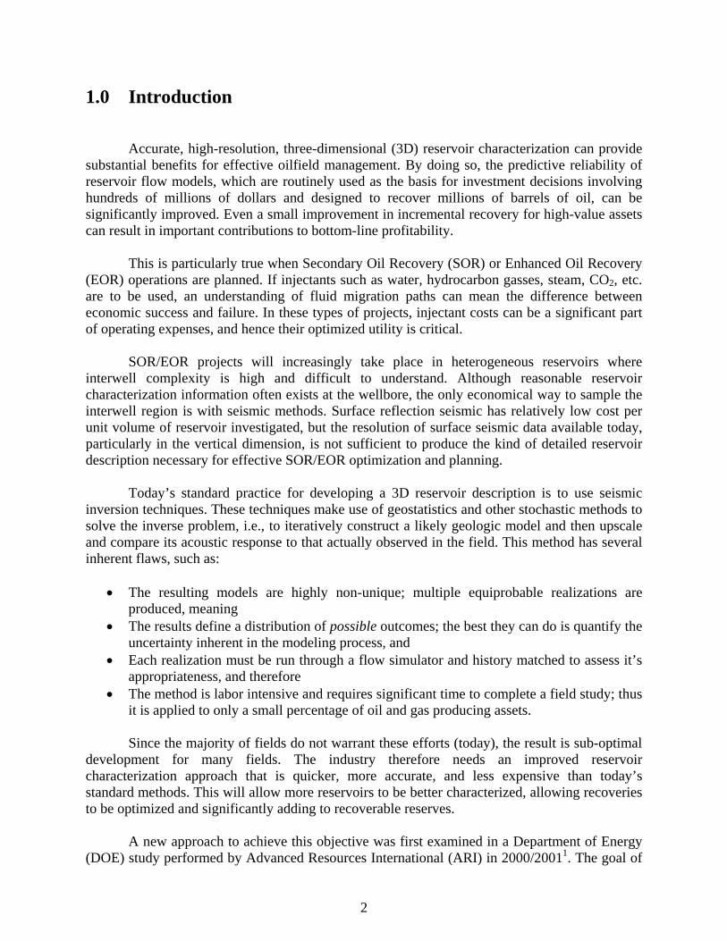
that study was to evaluate whether robust relationships between data at vastly different scales of measurement could be established using virtual intelligence (VI) methods. The proposed

Figure 1: Pathway to 3D High-Resolution Reservoir Description

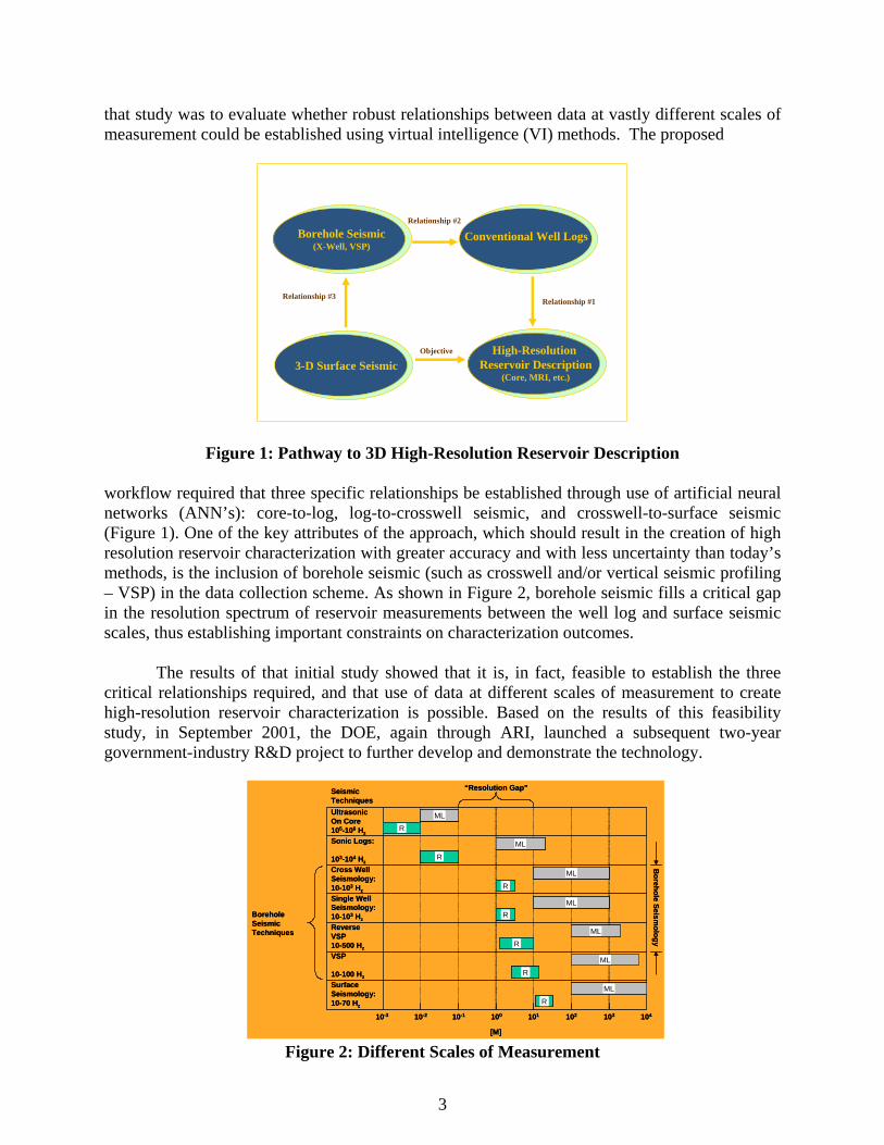
workflow required that three specific relationships be established through use of artificial neural networks (ANN’s): core-to-log, log-to-crosswell seismic, and crosswell-to-surface seismic (Figure 1). One of the key attributes of the approach, which should result in the creation of high resolution reservoir characterization with greater accuracy and with less uncertainty than today’s methods, is the inclusion of borehole seismic (such as crosswell and/or vertical seismic profiling – VSP) in the data collection scheme. As shown in Figure 2, borehole seismic fills a critical gap in the resolution spectrum of reservoir measurements between the well log and surface seismic scales, thus establishing important constraints on characterization outcomes.



Figure 2: Different Scales of Measurement

Borehole Seismic(X-Well, VSP)

Conventional Well Logs

3-D Surface SeismicHigh-Resolution

Reservoir Description(Core, MRI, etc.)

Objective

Relationship #3

Relationship #2

Relationship #1

Borehole Seismic(X-Well, VSP)

Conventional Well Logs

3-D Surface SeismicHigh-Resolution

Reservoir Description(Core, MRI, etc.)

Objective

Relationship #3

Relationship #2

Relationship #1

UltrasonicOn Core105-106 Hz

SeismicTechniques

Sonic Logs:

103-104 HzCross WellSeismology:10-103 HzSingle WellSeismology:10-103 HzReverseVSP10-500 HzVSP

10-100 HzSurfaceSeismology:10-70 Hz

BoreholeSeismicTechniques

R

R

R

R

R

R

ML

ML

ML

RML

ML

ML

ML

10-3 10-2 10-1 100 101 102 103 104

Borehole Seism

ology

[M]

“Resolution Gap”

UltrasonicOn Core105-106 Hz

SeismicTechniques

Sonic Logs:

103-104 HzCross WellSeismology:10-103 HzSingle WellSeismology:10-103 HzReverseVSP10-500 HzVSP

10-100 HzSurfaceSeismology:10-70 Hz

BoreholeSeismicTechniques

RRR

RRR

RRR

RRR

RRR

RRR

MLMLML

MLMLML

MLMLML

RRRMLMLML

MLMLML

MLMLML

MLMLML

10-3 10-2 10-1 100 101 102 103 104

Borehole Seism

ology

[M]

“Resolution Gap”

4




reservoir modeling or other statistical methods.

This report describes the results of that project.

5

2.0 Technical Approach 2.1 Analytic Workflow

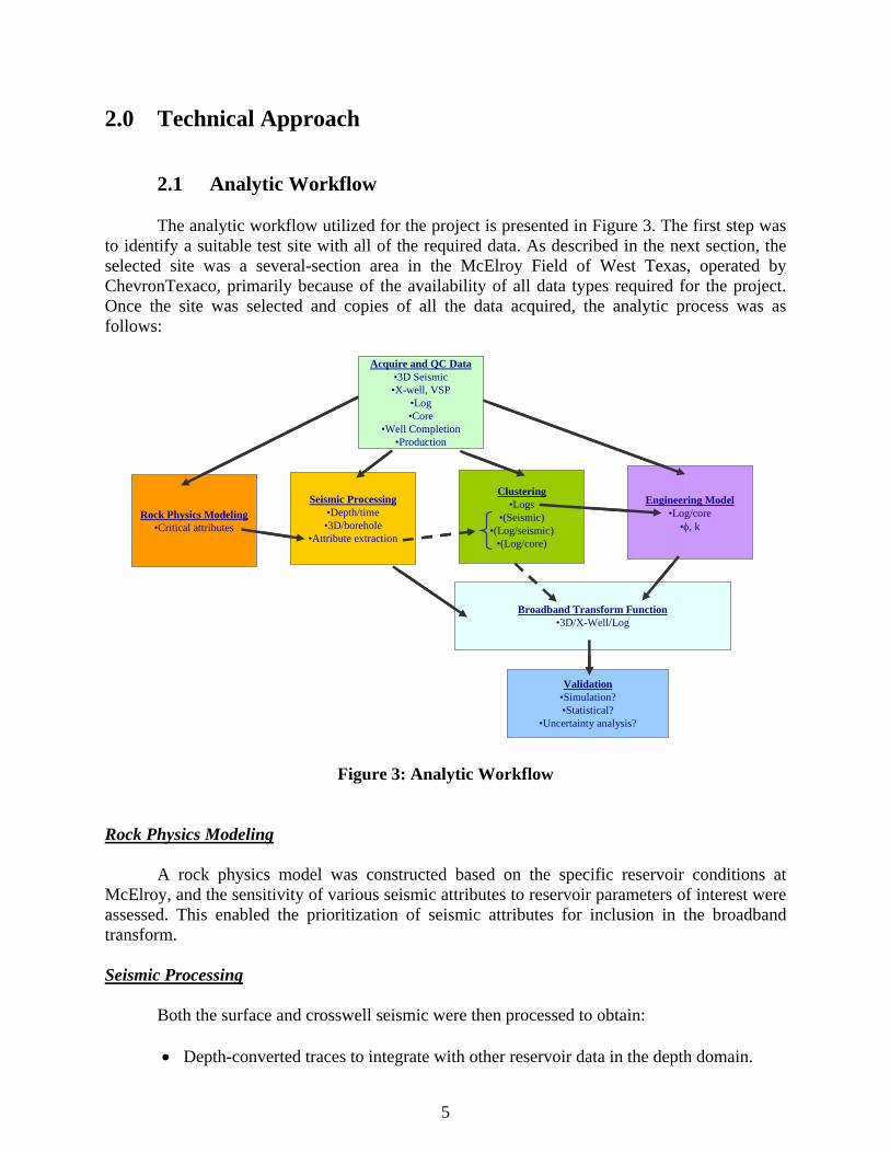
The analytic workflow utilized for the project is presented in Figure 3. The first step was

to identify a suitable test site with all of the required data. As described in the next section, the selected site was a several-section area in the McElroy Field of West Texas, operated by ChevronTexaco, primarily because of the availability of all data types required for the project. Once the site was selected and copies of all the data acquired, the analytic process was as follows:

Figure 3: Analytic Workflow

Rock Physics Modeling A rock physics model was constructed based on the specific reservoir conditions at

McElroy, and the sensitivity of various seismic attributes to reservoir parameters of interest were assessed. This enabled the prioritization of seismic attributes for inclusion in the broadband transform.

Seismic Processing

Both the surface and crosswell seismic were then processed to obtain: • Depth-converted traces to integrate with other reservoir data in the depth domain.

Acquire and QC Data•3D Seismic•X-well, VSP

•Log•Core

•Well Completion•Production

Clustering•Logs

•(Seismic)•(Log/seismic)

•(Log/core)

Seismic Processing•Depth/time•3D/borehole

•Attribute extraction

Rock Physics Modeling•Critical attributes

Engineering Model•Log/core

•φ, k

Broadband Transform Function•3D/X-Well/Log

Validation•Simulation?•Statistical?

•Uncertainty analysis?

Acquire and QC Data•3D Seismic•X-well, VSP

•Log•Core

•Well Completion•Production

Clustering•Logs

•(Seismic)•(Log/seismic)

•(Log/core)

Seismic Processing•Depth/time•3D/borehole

•Attribute extraction

Rock Physics Modeling•Critical attributes

Engineering Model•Log/core

•φ, k



Validation•Simulation?•Statistical?

•Uncertainty analysis?

6

• Co-located surface and crosswell traces such that they could be related to one another with correct spatial reference.

• Computation of prioritized attributes for both the surface and crosswell data. These data were then incorporated into the project database for analysis and the

development of the broadband transform function.

Clustering Prior to data analysis, clustering was performed on the data to establish another level of

data categorization, which was expected to enhance the predictive capability of the transform. Specifically, the well logs were clustered to establish lithologic units, and each depth interval assigned its appropriate lithology unit. Thus rather than only have log curve values as predictors of core properties, lithology was also an input parameter. This was used in the log-to-core transform.

Engineering Model

An engineering model was developed using ANN’s to predict core properties (porosity

and permeability) from log data. This model was to be used downstream of the broadband transform which would compute well logs from surface seismic data.

Broadband Transform Function

The broadband transform function was to utilize two cascading ANN’s to predict well log

responses from surface seismic data. Specifically, an ANN was constructed to predict the selected crosswell seismic attributes from the surface seismic attributes, and another ANN to compute well log responses from the computed crosswell attributes. Thus, these two models would be able to compute log responses at each surface seismic location, from which the engineering model would then compute porosity and permeability.

The following sections describe in more detail the procedures and results of each of these

analytic tasks. Note that topical reports have also been prepared for each task, which provide considerably more detail than provided herein and can be obtained by the interested reader.

7

2.2 Test Site Description and Data Availability The first step in the project was to locate a suitable test site. The merits of various

potential sites, including data availability, resource size, and operator cost-share, were considered before ultimately deciding upon the McElroy field, a large oil field in the Permian Basin of west Texas, operated by ChevronTexaco (Figure 4).

Figure 4: Major Grayburg Fields Along the Central Basin Platform Trend

McElroy was chosen because it met several important requirements:

• All data types required for the study were readily available, including surface (3D) seismic, crosswell seismic, modern logs and extensive core data.

• The operator (ChevronTexaco) was willing to work with the project team by providing access to proprietary data and technical personnel.

• Successful application of the technique could be immediately applied elsewhere in the field, as well as in nearby fields.

On the other hand, the producing horizon, the Grayburg formation, is a complex

carbonate reservoir. While it would have been preferred to test the new reservoir characterization approach in a less complex (e.g., clastic) reservoir, no such test site with all required information could be identified. Thus the McElroy field was selected as the test site for this study.

McElroy FieldMcElroy Field

8

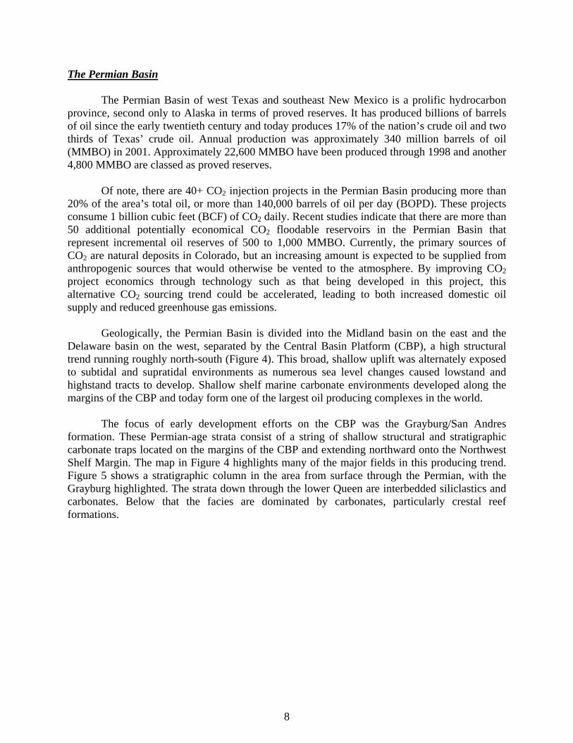
The Permian Basin

The Permian Basin of west Texas and southeast New Mexico is a prolific hydrocarbon province, second only to Alaska in terms of proved reserves. It has produced billions of barrels of oil since the early twentieth century and today produces 17% of the nation’s crude oil and two thirds of Texas’ crude oil. Annual production was approximately 340 million barrels of oil (MMBO) in 2001. Approximately 22,600 MMBO have been produced through 1998 and another 4,800 MMBO are classed as proved reserves.

Of note, there are 40+ CO2 injection projects in the Permian Basin producing more than

20% of the area’s total oil, or more than 140,000 barrels of oil per day (BOPD). These projects consume 1 billion cubic feet (BCF) of CO2 daily. Recent studies indicate that there are more than 50 additional potentially economical CO2 floodable reservoirs in the Permian Basin that represent incremental oil reserves of 500 to 1,000 MMBO. Currently, the primary sources of CO2 are natural deposits in Colorado, but an increasing amount is expected to be supplied from anthropogenic sources that would otherwise be vented to the atmosphere. By improving CO2 project economics through technology such as that being developed in this project, this alternative CO2 sourcing trend could be accelerated, leading to both increased domestic oil supply and reduced greenhouse gas emissions.

Geologically, the Permian Basin is divided into the Midland basin on the east and the

Delaware basin on the west, separated by the Central Basin Platform (CBP), a high structural trend running roughly north-south (Figure 4). This broad, shallow uplift was alternately exposed to subtidal and supratidal environments as numerous sea level changes caused lowstand and highstand tracts to develop. Shallow shelf marine carbonate environments developed along the margins of the CBP and today form one of the largest oil producing complexes in the world.

The focus of early development efforts on the CBP was the Grayburg/San Andres

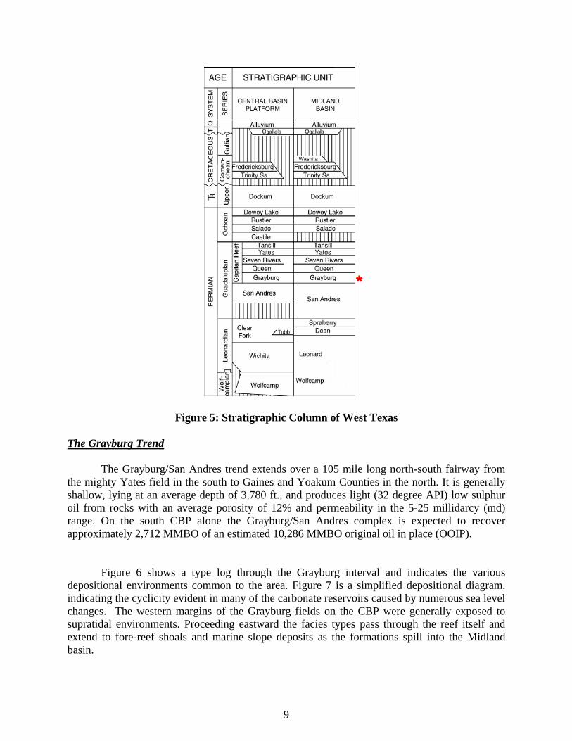
formation. These Permian-age strata consist of a string of shallow structural and stratigraphic carbonate traps located on the margins of the CBP and extending northward onto the Northwest Shelf Margin. The map in Figure 4 highlights many of the major fields in this producing trend. Figure 5 shows a stratigraphic column in the area from surface through the Permian, with the Grayburg highlighted. The strata down through the lower Queen are interbedded siliclastics and carbonates. Below that the facies are dominated by carbonates, particularly crestal reef formations.

9

Figure 5: Stratigraphic Column of West Texas

The Grayburg Trend

The Grayburg/San Andres trend extends over a 105 mile long north-south fairway from the mighty Yates field in the south to Gaines and Yoakum Counties in the north. It is generally shallow, lying at an average depth of 3,780 ft., and produces light (32 degree API) low sulphur oil from rocks with an average porosity of 12% and permeability in the 5-25 millidarcy (md) range. On the south CBP alone the Grayburg/San Andres complex is expected to recover approximately 2,712 MMBO of an estimated 10,286 MMBO original oil in place (OOIP).

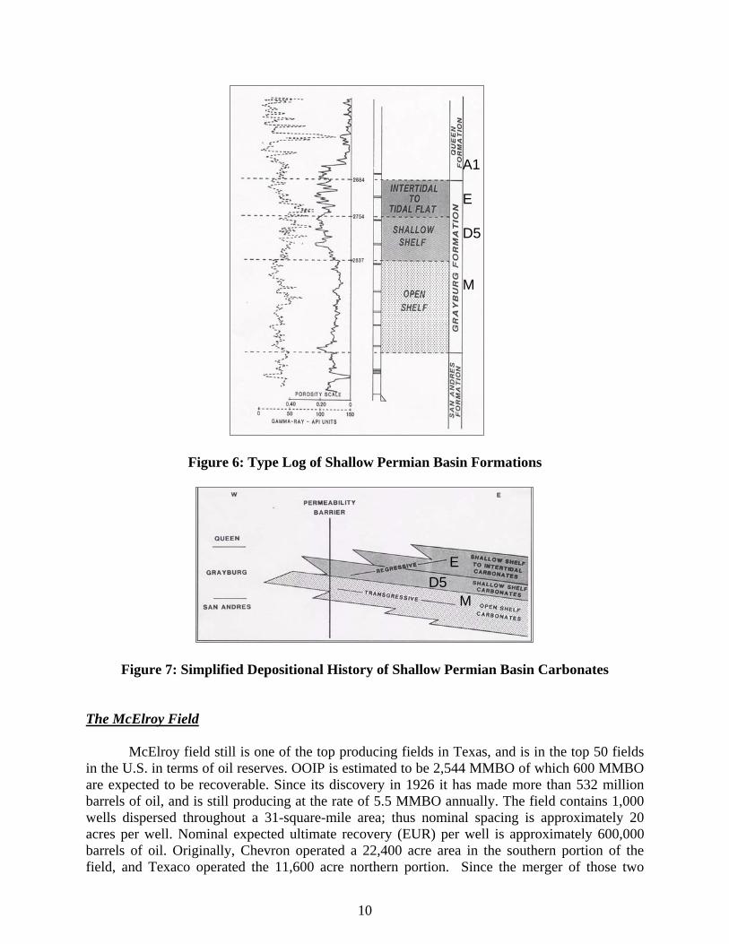
Figure 6 shows a type log through the Grayburg interval and indicates the various

depositional environments common to the area. Figure 7 is a simplified depositional diagram, indicating the cyclicity evident in many of the carbonate reservoirs caused by numerous sea level changes. The western margins of the Grayburg fields on the CBP were generally exposed to supratidal environments. Proceeding eastward the facies types pass through the reef itself and extend to fore-reef shoals and marine slope deposits as the formations spill into the Midland basin.

**

10

Figure 6: Type Log of Shallow Permian Basin Formations

Figure 7: Simplified Depositional History of Shallow Permian Basin Carbonates

The McElroy Field

McElroy field still is one of the top producing fields in Texas, and is in the top 50 fields in the U.S. in terms of oil reserves. OOIP is estimated to be 2,544 MMBO of which 600 MMBO are expected to be recoverable. Since its discovery in 1926 it has made more than 532 million barrels of oil, and is still producing at the rate of 5.5 MMBO annually. The field contains 1,000 wells dispersed throughout a 31-square-mile area; thus nominal spacing is approximately 20 acres per well. Nominal expected ultimate recovery (EUR) per well is approximately 600,000 barrels of oil. Originally, Chevron operated a 22,400 acre area in the southern portion of the field, and Texaco operated the 11,600 acre northern portion. Since the merger of those two

A1

E

D5

M

A1

E

D5

M

ED5

M

ED5

M

11

companies the entire 34,000 acre field has been under consolidated operatorship. Waterflooding operations began in the early 1960’s.

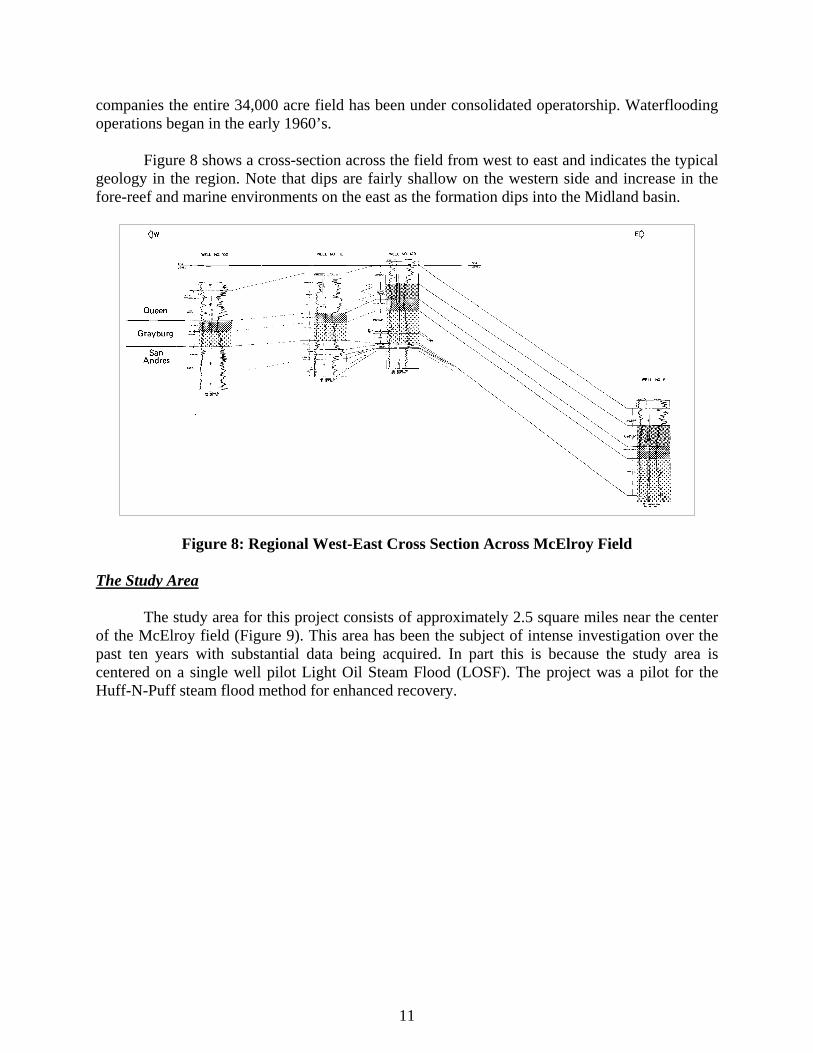
Figure 8 shows a cross-section across the field from west to east and indicates the typical

geology in the region. Note that dips are fairly shallow on the western side and increase in the fore-reef and marine environments on the east as the formation dips into the Midland basin.

Figure 8: Regional West-East Cross Section Across McElroy Field

The Study Area

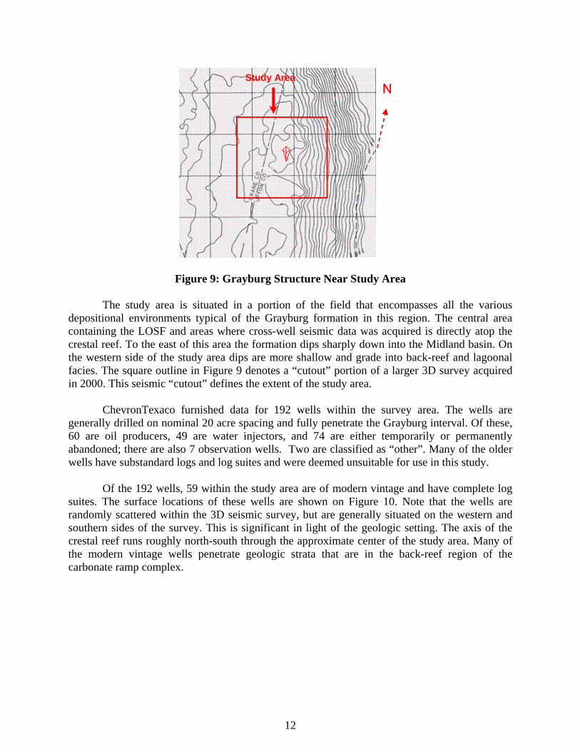
The study area for this project consists of approximately 2.5 square miles near the center of the McElroy field (Figure 9). This area has been the subject of intense investigation over the past ten years with substantial data being acquired. In part this is because the study area is centered on a single well pilot Light Oil Steam Flood (LOSF). The project was a pilot for the Huff-N-Puff steam flood method for enhanced recovery.

12

Figure 9: Grayburg Structure Near Study Area

The study area is situated in a portion of the field that encompasses all the various

depositional environments typical of the Grayburg formation in this region. The central area containing the LOSF and areas where cross-well seismic data was acquired is directly atop the crestal reef. To the east of this area the formation dips sharply down into the Midland basin. On the western side of the study area dips are more shallow and grade into back-reef and lagoonal facies. The square outline in Figure 9 denotes a “cutout” portion of a larger 3D survey acquired in 2000. This seismic “cutout” defines the extent of the study area.

ChevronTexaco furnished data for 192 wells within the survey area. The wells are generally drilled on nominal 20 acre spacing and fully penetrate the Grayburg interval. Of these, 60 are oil producers, 49 are water injectors, and 74 are either temporarily or permanently abandoned; there are also 7 observation wells. Two are classified as “other”. Many of the older wells have substandard logs and log suites and were deemed unsuitable for use in this study.

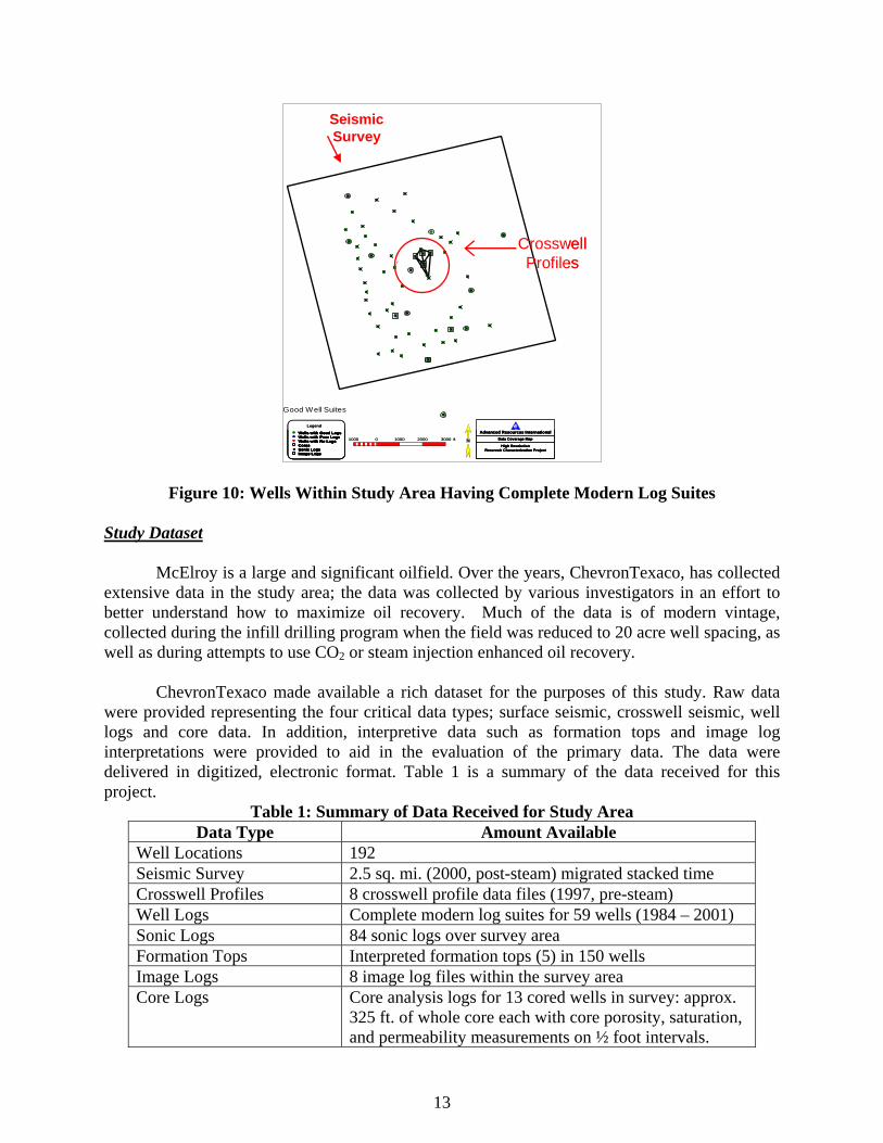
Of the 192 wells, 59 within the study area are of modern vintage and have complete log

suites. The surface locations of these wells are shown on Figure 10. Note that the wells are randomly scattered within the 3D seismic survey, but are generally situated on the western and southern sides of the survey. This is significant in light of the geologic setting. The axis of the crestal reef runs roughly north-south through the approximate center of the study area. Many of the modern vintage wells penetrate geologic strata that are in the back-reef region of the carbonate ramp complex.

Study AreaN

Study AreaN

13

Figure 10: Wells Within Study Area Having Complete Modern Log Suites

Study Dataset

McElroy is a large and significant oilfield. Over the years, ChevronTexaco, has collected extensive data in the study area; the data was collected by various investigators in an effort to better understand how to maximize oil recovery. Much of the data is of modern vintage, collected during the infill drilling program when the field was reduced to 20 acre well spacing, as well as during attempts to use CO2 or steam injection enhanced oil recovery.

ChevronTexaco made available a rich dataset for the purposes of this study. Raw data were provided representing the four critical data types; surface seismic, crosswell seismic, well logs and core data. In addition, interpretive data such as formation tops and image log interpretations were provided to aid in the evaluation of the primary data. The data were delivered in digitized, electronic format. Table 1 is a summary of the data received for this project.

Table 1: Summary of Data Received for Study Area Data Type Amount Available

Well Locations 192 Seismic Survey 2.5 sq. mi. (2000, post-steam) migrated stacked time Crosswell Profiles 8 crosswell profile data files (1997, pre-steam) Well Logs Complete modern log suites for 59 wells (1984 – 2001) Sonic Logs 84 sonic logs over survey area Formation Tops Interpreted formation tops (5) in 150 wells Image Logs 8 image log files within the survey area Core Logs Core analysis logs for 13 cored wells in survey: approx.

325 ft. of whole core each with core porosity, saturation, and permeability measurements on ½ foot intervals.

Advanced Resources InternationalData Coverage Map

High ResolutionReservoir Characterization Project



Wells with Good LogsWells with Poor LogsWells with No LogsCoresSonic LogsImage Logs

Legend



Legend

Good Well Suites

1000 0 1000 2000 3000 ft

Seismic Survey

CrosswellProfiles






Legend



Legend

Good Well Suites

1000 0 1000 2000 3000 ft

Seismic Survey

CrosswellProfiles

14

Surface and crosswell seismic data was acquired in several programs before and after the initiation of a single–well LOSF pilot conducted in the central well of the cross-well seismic data area. This single well pilot used the Huff-N-Puff method with a period of steam injection followed by a period of oil production from the same well. In a true Huff-N-Puff project this cycle would be repeated over and over again. At McElroy only a single steam injection cycle was conducted.

Surface seismic data was acquired before and after steam injection. Only the 2000-

vintage (post-steam) survey was available for this study. However, due to the small volume of steam injected and (very) limited overall effect, most of the area with coincident crosswell and surface seismic data was believed to be largely unaffected by the steam, and hence deemed suitable for correlation in this study.

The surface seismic consists of about 30,000 traces of time-migrated, stacked P-P

amplitudes on 55 ft. by 55 ft. bin spacing. There are 175 inlines and 175 crosslines. Trace gathers were later obtained, but the quality is poor. The gathers were used, however, to pick first arrivals to aid in the seismic time-to-depth conversion process.

The crosswell profile data was obtained between six wells in the center of the study area,

with the central well being the LOSF pilot well (Figure 10). Data quality varies between profiles, with the shorter profiles having the best quality. The source was piezeo-electric and the receiver array had 55 clamped geophones. The crosswell data used in this study was the set acquired before steam injection.

In terms of geophysical well logs, Table 2 summarizes the curves that comprise a

complete log suite for the purposes of this study. Each of the 59 selected wells contain full coverage for all six log data types across the entire Grayburg interval, some 350 feet per well. These additional log data, such as the density porosity log (DPHI), were not used in this analysis, however, because they are not available for all the wells.

Table 2: Log Data Type Summary

Data Type Abbreviation Units Indicator Gamma Ray GR API units Shaliness Compensated Neutron Log CNL Percent Porosity Bulk density Log RHOB gm/cc Porosity Sonic Travel Time DT usec/ft Porosity Photoelectric Effect PE barns/m2 Mineralogy Latero-Log LLD Ohm-m Resistivity

2.3 Rock Physics Modeling

As described above, the project dataset consisted of a large suite of logs, some core data,

and both surface 3D and interwell seismic surveys. Because of the significant difference in levels of resolution available from surface seismic data (lowest level of resolution), borehole seismic

15

data (much higher level of resolution), and core and log data (highest level of resolution), the borehole seismic data was used as an intermediate means of extending the resolution level of the much more extensive surface seismic data when building a model of the McElroy reservoir.

Attributes can be computed from either surface or borehole seismic data using specific

computational algorithms which can help to enhance or detect certain information which is often hidden, but inherent within the seismic data. In order to establish the relationships between information available from the seismic data and reservoir properties, rock physics approaches were utilized. Today rock physics is a viable and active area of study, and many useful theoretical relationships, as well as physical measurements of rock and fluid properties are known and available for use. Among these are the well-known Biot-Gassmann relations which establish relationships between shear and compressional wave velocities, and rock and fluid moduli and densities as well as porosity of the reservoir rock. Using these relationships, the effect of changes in any of these reservoir parameters on the recorded seismic data can be predicted. These relationships can also be used as a basis for modeling the actual seismic response of the reservoir which can in turn, be used to evaluate the sensitivity in response of the various seismic attributes to these changes. On this basis, those attributes which are most sensitive to change and then used for building the reservoir characterization model.

A very specific rock physics model of the McElroy reservoir was constructed, allowing

us to predict with some accuracy the required bulk and shear moduli and densities of the reservoir rock as a function of mineralogy (primarily carbonate) and porosity. Similar estimates of bulk moduli and density of composite pore fluids (typically water/oil/brine or gas) were also made. Having made these estimates, these quantities were entered into the Biot-Gassmann relations in order to obtain relationships between these quantities and the resulting shear and compressional seismic velocities of the porous fluid-saturated reservoir rock.

Entering specific rock and fluid parameters into the Biot-Gassmann relations leads to

very organized sets of results which have been catalogued in the form of charts showing relationships between various rock and fluid properties and seismic data properties. In particular, we have organized a fairly large volume of rock physics data into charts which detail the relationship of seismic parameters including shear and compressional wave velocities, and shear and compressional wave acoustic impedances as a function of porosity for specific pore fluids and mineralogies. By varying the pore fluid or mineralogies, we then generated multiple curves which allowed us to evaluate the degree of sensitivity of specific seismic parameters to changes in mineralogy or pore fluid content, indexed by a range of values of porosity. Taken together, they give a very complete picture of dependencies between seismic parameters and the various rock and fluid properties, including porosity, mineralogy, and pore fluid.

In addition to the computational rock physics models, a number of detailed models of the

McElroy reservoir were built using log and core data, but based on the effect of the individual units on seismic response. Since it is ultimately true that seismic data responds directly to changes in acoustic impedance, these models are based on acoustic impedance estimates obtained from log and core data. They differ in complexity, based on the level of dominance of the interfaces separating units when viewed as seismic reflectors (interfaces where acoustic impedance shows a significant change). The simplest models consist of units which have the greatest effect on reflection seismic data, and these units are then subdivided into units at a finer scale, which have a diminished effect on the recorded reflection seismic data.

16

In order to use the considerable amount of rock physics data available from these various models to evaluate changes in seismic response, and sensitivity of attributes to these changes, a means is required for simulating the seismic data which would result from a specific reservoir model. As a result, we have made use of very sophisticated elastic seismic modeling code which allowed us to input a detailed elastic reservoir model, and to simulate the seismic response from the model. This capability allowed us to very accurately simulate both shear and compressional wave data, and allowed us to further evaluate the effects of seismic response as a function of offset (AVO response).

The seismic modeling code assumes an isotropic elastic earth model which obeys

Hooke’s Law. This means that the model is ultimately entered in terms of the elastic Lame’ parameters at each point in the model. These Lame’ parameters can be computed from a knowledge of bulk and shear moduli, which become available from our rock physics computations, based either on specified reservoir rock and fluid properties, or similar input data derived from log and core analysis. We should point out that the seismic modeling code also allows the capability of specifying a complete Q (frequency dependent attenuation) model for the reservoir, but without good Q data available from a VSP survey, for example, we have used a default constant Q model in our work.

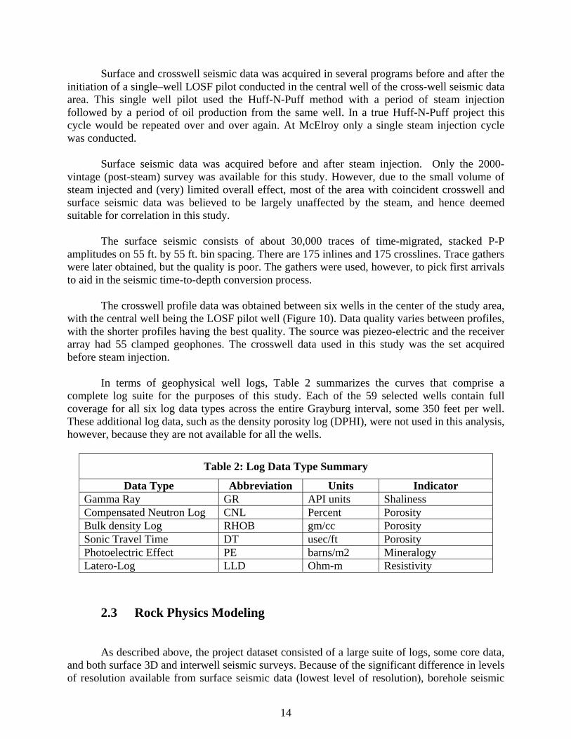
Using all of these capabilities, a large number of models were run, resulting in a number

of synthetic data sets which allowed us to test the response of different attributes to specific levels of change in mineralogy, porosity, and pore fluid content, as well as to complexity of the models. These synthetic data sets were then used to compute and evaluate a reasonably large number of standard seismic attributes. We then applied several different measures to determine sensitivity of response of the attributes to specific changes in the model. These were evaluated, and on the basis of this work, ten seismic attributes were chosen for use in our subsequent analysis of the McElroy data, Figure 11.

Figure 11: Responses of Various Attributes to Changes in Porosity of 5%, 10%, and 15%

in the Biot-Gassmann Layer

17

The ten attributes which were chosen are listed below, with a brief description, where appropriate: • Trace Differentiation • Hilbert Transform (complex part of the analytic trace) • Perigram (zero mean of the complex amplitude of the trace) • Cosine of Phase (cosine of the instantaneous phase) • Perigram * Cosine of Phase (product of these two attributes) • Instantaneous Phase • Instantaneous Frequency (time derivative of instantaneous phase) • Median Smoother (3 point) • Absolute Value of Trace • Response Phase (instantaneous phase at the trace envelope peaks, in degrees)

A complete topical report has been prepared on this work and can be obtained via the references2.

2.4 Seismic Data Processing

As elaborated upon elsewhere, the goal was to establish relationships between data of different scales using ANN’s for the purpose of improved reservoir characterization. The data range from very fine-scale core measurements to very coarse-scale surface seismic measurements connected in between by log and crosswell seismic data. The data provided by ChevronTexaco consisted of a small (1.8 by 1.8 mile), 3D, surface seismic survey recorded at the McElroy field by Dawson Geophysical, and a total of 8 crosswell seismic profiles recorded by TomoSeis Inc.; both datasets were acquired under contract with ChevronTexaco. The crosswell profiles are located near the center to the surface survey.

The crosswell and surface data integration comprised three main tasks. 1. Process two of the crosswell datasets to derive a high-resolution reflection image

along profiles between the source and receiver wells. 2. Interpolate and resample the 3D surface data in order to create a reflection image

that is collocated, trace-for-trace, with the reflection image produced from the crosswell data. 3. Convert the 3D, surface survey from time to depth, which required computing a

3D velocity model using the available sonic logs and the normal moveout velocities of the seismic data.

The trace spacing of the surface data was 55 feet, approximately an order of magnitude

coarser than that of the crosswell data. The very good data quality plus the low structural relief within the McElroy field allowed for the projection of the surface traces onto the crosswell trace locations by straightforward linear interpolation. The interpolation was carried out along the structural strike and dip as computed from the seismic data In addition the surface data were converted from a time-sample interval of 2 msec to a depth-sample interval of 0.5 feet to

18

conform with the vertical scale of the crosswell image. Low structural relief at McElroy also allowed the time to depth conversion to be carried out by a simple one-dimensional rescaling of the traces.

Co-locating the surface traces to the crosswell traces and converting from time to depth

are felt to be quite accurate given the excellent quality of the surface data, the dense well control, and the low relief of the McElroy structure. The need to use normal moveout velocities for depths above the log measurements was also acceptable and provided a good initial alignment of the seismic and well log data. The final alignment was obtained by crosscorrelation between the real and sonic-log-generated synthetic traces. The alignments were smoothly varying across the survey area as would be expected if such variations were caused by corresponding variations in the near-surface velocity. The crosscorrelation itself ranged from good to fair, but the strong reflections at the Queen and M markers helped make the alignments unambiguous.

The crosswell data were more difficult to analyze due to the high level of tube wave

noise. Nevertheless reflection images were computed with a much broader frequency bandwidth and consequently a much greater resolution when compared to the surface data. The crosswell reflection images were also nosier and contained many short segments of coherent energy, which are probably artifacts of the heavy-duty filtering required to attenuate the tube waves. The A1 and M reflectors could be correlated between the two datasets, but the character of the reflection waveforms was, as expected, very different.

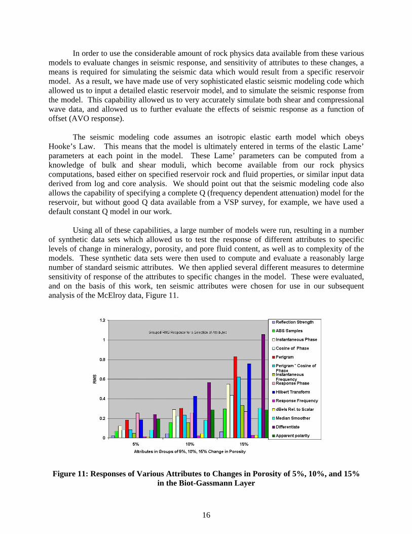
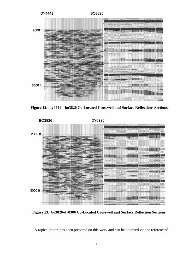
The crosswell data quality was in general poor, and the reflection image is much nosier

than the corresponding image from the surface data, although it is of much higher resolution. There are several reflectors that can be correlated between the two images, notably the A1 and M horizons within the Grayburg Formation. Otherwise the two images are remarkably different, although this is not surprising given the broader frequency bandwidth and higher noise level in the crosswell data, as shown in Figures 12 and 13.

19

Figure 12: dy4441 – bo3826 Co-Located Crosswell and Surface Reflections Sections

Figure 13: bo3826-dy0386 Co-Located Crosswell and Surface Reflection Sections

A topical report has been prepared on this work and can be obtained via the references3.

2000 ft.

3000 ft

DY4441 BO3826

2000 ft.

3000 ft

DY4441 BO3826

2000 ft.

3000 ft

BO3826 DY0386

2000 ft.

3000 ft

BO3826 DY0386

20

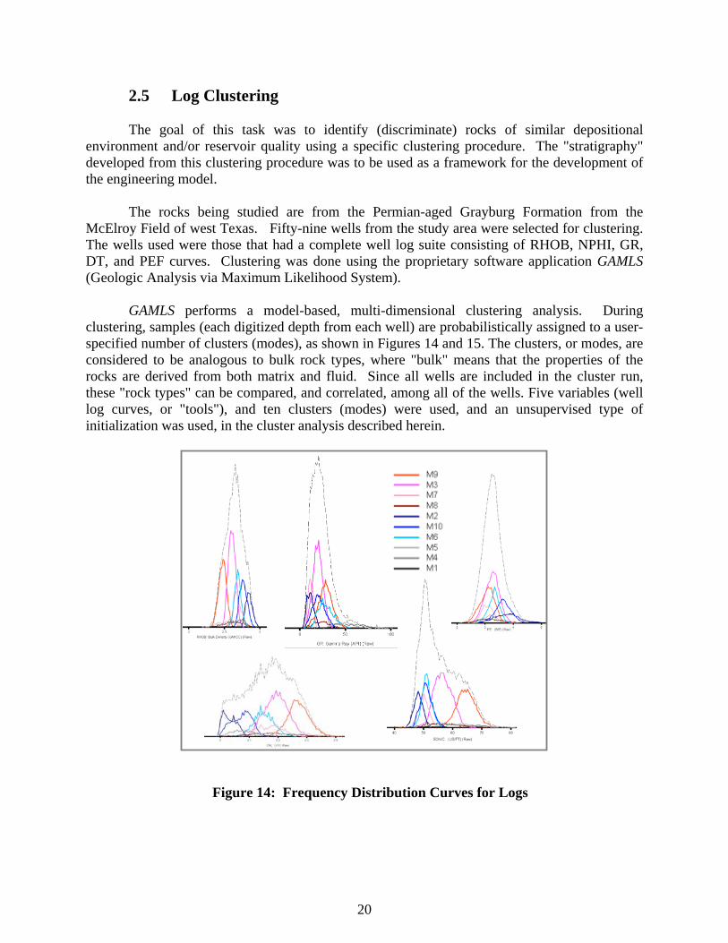
2.5 Log Clustering The goal of this task was to identify (discriminate) rocks of similar depositional

environment and/or reservoir quality using a specific clustering procedure. The "stratigraphy" developed from this clustering procedure was to be used as a framework for the development of the engineering model.

The rocks being studied are from the Permian-aged Grayburg Formation from the

McElroy Field of west Texas. Fifty-nine wells from the study area were selected for clustering. The wells used were those that had a complete well log suite consisting of RHOB, NPHI, GR, DT, and PEF curves. Clustering was done using the proprietary software application GAMLS (Geologic Analysis via Maximum Likelihood System).

GAMLS performs a model-based, multi-dimensional clustering analysis. During

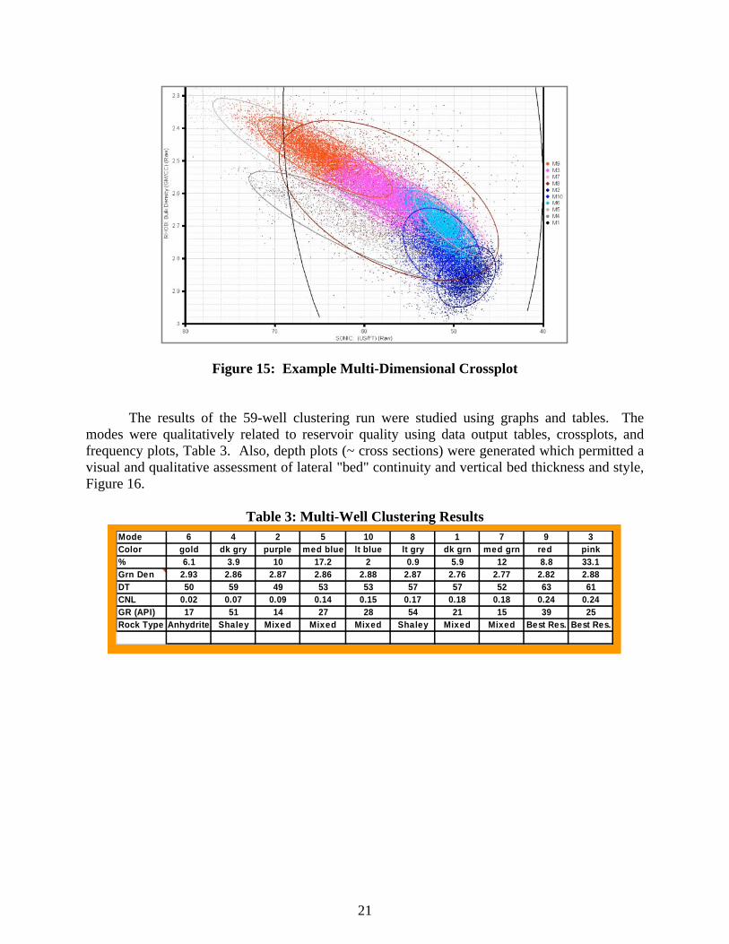
clustering, samples (each digitized depth from each well) are probabilistically assigned to a user-specified number of clusters (modes), as shown in Figures 14 and 15. The clusters, or modes, are considered to be analogous to bulk rock types, where "bulk" means that the properties of the rocks are derived from both matrix and fluid. Since all wells are included in the cluster run, these "rock types" can be compared, and correlated, among all of the wells. Five variables (well log curves, or "tools"), and ten clusters (modes) were used, and an unsupervised type of initialization was used, in the cluster analysis described herein.

Figure 14: Frequency Distribution Curves for Logs

21

Figure 15: Example Multi-Dimensional Crossplot

The results of the 59-well clustering run were studied using graphs and tables. The

modes were qualitatively related to reservoir quality using data output tables, crossplots, and frequency plots, Table 3. Also, depth plots (~ cross sections) were generated which permitted a visual and qualitative assessment of lateral "bed" continuity and vertical bed thickness and style, Figure 16.

Table 3: Multi-Well Clustering Results

Mode 6 4 2 5 10 8 1 7 9 3Color gold dk gry purple med blue lt blue lt gry dk grn med grn red pink% 6.1 3.9 10 17.2 2 0.9 5.9 12 8.8 33.1Grn Den 2.93 2.86 2.87 2.86 2.88 2.87 2.76 2.77 2.82 2.88DT 50 59 49 53 53 57 57 52 63 61CNL 0.02 0.07 0.09 0.14 0.15 0.17 0.18 0.18 0.24 0.24GR (API) 17 51 14 27 28 54 21 15 39 25Rock Type Anhydrite Shaley Mixed Mixed Mixed Shaley Mixed Mixed Best Res. Best Res.

Mode 6 4 2 5 10 8 1 7 9 3Color gold dk gry purple med blue lt blue lt gry dk grn med grn red pink% 6.1 3.9 10 17.2 2 0.9 5.9 12 8.8 33.1Grn Den 2.93 2.86 2.87 2.86 2.88 2.87 2.76 2.77 2.82 2.88DT 50 59 49 53 53 57 57 52 63 61CNL 0.02 0.07 0.09 0.14 0.15 0.17 0.18 0.18 0.24 0.24GR (API) 17 51 14 27 28 54 21 15 39 25Rock Type Anhydrite Shaley Mixed Mixed Mixed Shaley Mixed Mixed Best Res. Best Res.

22

Figure 16: Cluster Assignments Compared to Core Data

The three modes (clusters) with the best reservoir quality were identified on the basis of

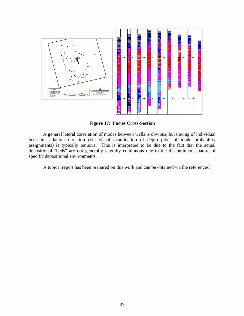
apparent porosity (from mean NPHI) and apparent clay content (from mean GR). These three modes were dominant in the depth ranges between the E and M Grayburg stratigraphic markers. The poorest reservoir quality was in modes that were dominant below the M stratigraphic marker. Porosity and permeability values obtained from plugs from the cored well (DY0534) nearest to the crosswell seismic area show a similar depth zonation. Thus, the relative reservoir quality inferred from the clustering analysis agrees with the results of empirical measurements made on the whole core in terms of overall zonation of the Grayburg Formation, Figure 17.

Facies Porosity PermeabilityFacies Porosity Permeability

23

Figure 17: Facies Cross-Section

A general lateral correlation of modes between wells is obvious, but tracing of individual

beds in a lateral direction (via visual examination of depth plots of mode probability assignments) is typically tenuous. This is interpreted to be due to the fact that the actual depositional "beds" are not generally laterally continuous due to the discontinuous nature of specific depositional environments.


24

3.0 Results and Discussion

3.1 Log-Core Model The relationship between well logs and core parameters is strongly non-linear,

particularly in non-clastic, carbonate rocks such as the Grayburg. With log and core values measured at half-foot intervals in ten wells, a large volume of data was available for analysis (approximately 6,000 data points – 10 wells x 300 ft/well x ½ ft measurement interval). These two attributes of the dataset (complex relationship and large volume of data) suggest ANN’s can be an effective method to model the core-to-log relationship.

The strategy for creation of the model consisted of four steps:

1. Construct an ANN model and train it using data from cored wells. 2. Test the model during training to ensure that it is not memorizing test patterns. 3. Validate the trained network using data from cored wells that has not previously been

presented to the network. 4. Use the trained network to predict core values in wells that do not have whole core

samples available.

In keeping with standard practice described in the literature, the sample data set was broken into subsets consisting of 60% of data used for training, 20% of data used for testing, and 20% of data used for validation.

Two constraints guided the architectural structure of the ANN used in this analysis:

1. The network must generate predictions of porosity and permeability simultaneously. This constraint was imposed by the requirements of the global process which calls for simple methods of reservoir characterization. (If we were to create individual models for each core parameter, then for each individual log (from crosswell data), then for each crosswell attribute (from 3D data), the ultimate workflow would be much more burdensome than desired).

2. The network must be able to reliably generalize from training data to the prediction

mode. This constraint dictates that the internal structure of the neural network be relatively simple, with the fewest hidden node layers possible.

The imposition of these two constraints helped narrow the range of possible ANN

architectures. The optimal architecture was determined to be a three layer model with one input layer, one hidden layer, and one output layer. The input well logs were “depth windowed,” effectively tripling the apparent number of network inputs based on well logs. Although only six input log types were used the effect is to triple the number of log inputs to eighteen. While this makes the network architecture appear more complicated there are still only six types of log data being used as input. As previously stated, the output layer consisted of both target values, core porosity and permeability.

25

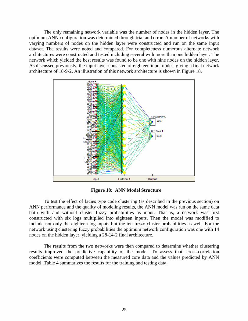
The only remaining network variable was the number of nodes in the hidden layer. The optimum ANN configuration was determined through trial and error. A number of networks with varying numbers of nodes on the hidden layer were constructed and run on the same input dataset. The results were noted and compared. For completeness numerous alternate network architectures were constructed and tested including several with more than one hidden layer. The network which yielded the best results was found to be one with nine nodes on the hidden layer. As discussed previously, the input layer consisted of eighteen input nodes, giving a final network architecture of 18-9-2. An illustration of this network architecture is shown in Figure 18.

Figure 18: ANN Model Structure

To test the effect of facies type code clustering (as described in the previous section) on

ANN performance and the quality of modeling results, the ANN model was run on the same data both with and without cluster fuzzy probabilities as input. That is, a network was first constructed with six logs multiplied into eighteen inputs. Then the model was modified to include not only the eighteen log inputs but the ten fuzzy cluster probabilities as well. For the network using clustering fuzzy probabilities the optimum network configuration was one with 14 nodes on the hidden layer, yielding a 28-14-2 final architecture.

The results from the two networks were then compared to determine whether clustering

results improved the predictive capability of the model. To assess that, cross-correlation coefficients were computed between the measured core data and the values predicted by ANN model. Table 4 summarizes the results for the training and testing data.

26

Table 4: Summary of Correlation Coefficients Between Measured Data and Values

Predicted by ANN’s With and Without Fuzzy Clustering Probabilities as Input

Parameter With Fuzzy Probabilities Without Fuzzy Probabilities

Porosity 0.863 0.855

Permeability 0.843 0.822

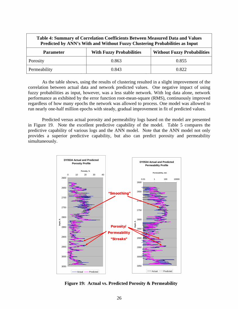
As the table shows, using the results of clustering resulted in a slight improvement of the correlation between actual data and network predicted values. One negative impact of using fuzzy probabilities as input, however, was a less stable network. With log data alone, network performance as exhibited by the error function root-mean-square (RMS), continuously improved regardless of how many epochs the network was allowed to process. One model was allowed to run nearly one-half million epochs with steady, gradual improvement in fit of predicted values.

Predicted versus actual porosity and permeability logs based on the model are presented in Figure 19. Note the excellent predictive capability of the model. Table 5 compares the predictive capability of various logs and the ANN model. Note that the ANN model not only provides a superior predictive capability, but also can predict porosity and permeability simultaneously.

Figure 19: Actual vs. Predicted Porosity & Permeability

DY0534 Actual and Predicted Porosity Profile

2600

2650

2700

2750

2800

2850

2900

2950

3000

3050

0 10 20 30 40

Porosity, %

Dep

th, f

t.

Actual Predicted

DY0534 Actual and Predicted Permeability Profile

2600

2650

2700

2750

2800

2850

2900

2950

3000

3050

0.01 1 100 10000

Permeability, md.

Dep

th, f

t.

Actual Predicted

“Smoothing”

Porosity/

Permeability

“Streaks”

DY0534 Actual and Predicted Porosity Profile

2600

2650

2700

2750

2800

2850

2900

2950

3000

3050

0 10 20 30 40

Porosity, %

Dep

th, f

t.

Actual Predicted

DY0534 Actual and Predicted Permeability Profile

2600

2650

2700

2750

2800

2850

2900

2950

3000

3050

0.01 1 100 10000

Permeability, md.

Dep

th, f

t.

Actual Predicted

“Smoothing”

Porosity/

Permeability

“Streaks”

27

Table 5: Benefits of ANN Model

This task has demonstrated that core porosity and permeability can be effectively predicted from geophysical log data using ANN’s to provide a high (vertical) resolution reservoir characterization for subsequent flow modeling and field development optimization.


3.2 Broadband Transform using Artificial Neural Networks

In this task, the possibility of designing a multi-scale transform which would accept 3D surface seismic data and a set of computed attributes as input, and would produce estimates of six well logs at each surface seismic bin location as output, was investigated. The transform itself was constructed from neural networks. Specifically, the program design included two neural networks. The first transformed 3D surface seismic depth converted data and their attributes into estimates of depth converted crosswell reflection data and their attributes. The second neural network was designed to transform the crosswell reflection data and their attributes into estimates of six specific well logs. When applied in cascade, the two neural networks effectively transformed surface seismic data and their computed attributes into estimates of six well logs at every 3D seismic bin location. The attributes used were selected as a result of analyzing synthetic data generated using rock physics models designed for this specific reservoir.

When this program, as originally conceived, was carried out, results were not sufficiently

good to warrant their use for the purposes of reservoir characterization. Numerous issues were identified which may have played a role in preventing the goals from being reached, and attempts were made to resolve them successfully. In the end, the desired goal of finding a transform using two cascaded neural networks which would accept 3D surface seismic data as input and produce estimates of six logs as output, was not achieved.

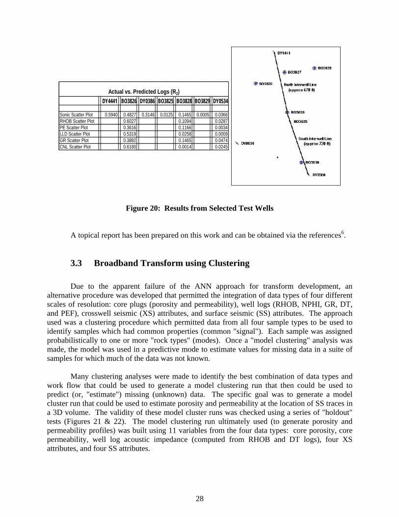
As Figure 20 illustrates, modest predictability of logs was achieved at the center well, but

these predictions significantly worsened for the outer wells. Therefore, the development of a transform using two cascading ANN’s, as originally conceived was not successful.

0.170.67DP log

0.710.74ANN Model

0.130.58RHOB log

0.020.24PE log

0.010.10LLD log

<0.010.02GR log

0.090.54CNL log

PermeabilityPorosityCorrelation R2Predictor

0.170.67DP log

0.680.73ANN Model

0.130.58RHOB log

0.020.24PE log

0.010.10LLD log

<0.010.02GR log

0.090.54CNL log


0.170.67DP log

0.710.74ANN Model

0.130.58RHOB log

0.020.24PE log

0.010.10LLD log

<0.010.02GR log

0.090.54CNL log


0.170.67DP log

0.680.73ANN Model

0.130.58RHOB log

0.020.24PE log

0.010.10LLD log

<0.010.02GR log

0.090.54CNL log


28

Figure 20: Results from Selected Test Wells A topical report has been prepared on this work and can be obtained via the references6. 3.3 Broadband Transform using Clustering

Due to the apparent failure of the ANN approach for transform development, an alternative procedure was developed that permitted the integration of data types of four different scales of resolution: core plugs (porosity and permeability), well logs (RHOB, NPHI, GR, DT, and PEF), crosswell seismic (XS) attributes, and surface seismic (SS) attributes. The approach used was a clustering procedure which permitted data from all four sample types to be used to identify samples which had common properties (common "signal"). Each sample was assigned probabilistically to one or more "rock types" (modes). Once a "model clustering" analysis was made, the model was used in a predictive mode to estimate values for missing data in a suite of samples for which much of the data was not known.

Many clustering analyses were made to identify the best combination of data types and

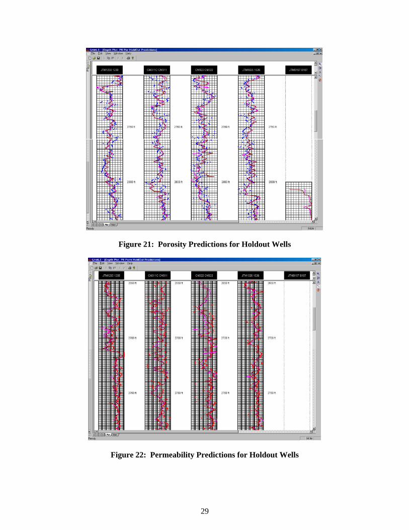
work flow that could be used to generate a model clustering run that then could be used to predict (or, "estimate") missing (unknown) data. The specific goal was to generate a model cluster run that could be used to estimate porosity and permeability at the location of SS traces in a 3D volume. The validity of these model cluster runs was checked using a series of "holdout" tests (Figures 21 & 22). The model clustering run ultimately used (to generate porosity and permeability profiles) was built using 11 variables from the four data types: core porosity, core permeability, well log acoustic impedance (computed from RHOB and DT logs), four XS attributes, and four SS attributes.

DY4441 BO3826 DY0386 BO3825 BO3828 BO3829 DY0534

Sonic Scatter Plot 0.5940 0.4827 0.3146 0.0125 0.1465 0.0005 0.0366RHOB Scatter Plot 0.6027 0.1094 0.0287PE Scatter Plot 0.3616 0.1166 0.0034LLD Scatter Plot 0.5319 0.0258 0.0009GR Scatter Plot 0.3882 0.1465 0.0474CNL Scatter Plot 0.6180 0.0014 0.0245

Actual vs. Predicted Logs (R2)

29

Figure 21: Porosity Predictions for Holdout Wells

Figure 22: Permeability Predictions for Holdout Wells

30

The model clustering used data from 15 wells: five cored wells with SS data, six cored wells with no SS data, and 3 wells located at the ends of two XS lines (one of the XS wells was used twice, with different sets of XS data). For all wells, the SS traces closest to the wells were used. The combination of the various data types generated from these 15 wells permitted the generation of the model clustering run that was used. The depth interval for which the model clustering run was developed and over which estimates of P&P were then made was about 350 feet. Core data indicated that the porosity generally increased down-section in the upper part of this interval and then decreased through the lower part of this interval. The core permeability followed a trend similar to the core porosity. However, these changes were not smooth with depth because of the thin-bedded nature of flow units. The well logs do not have the vertical resolution to "see" these small-scale changes in porosity and permeability, and also the SS traces do not "see" these changes.

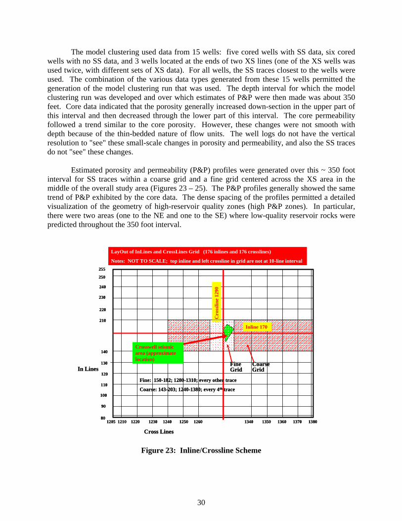
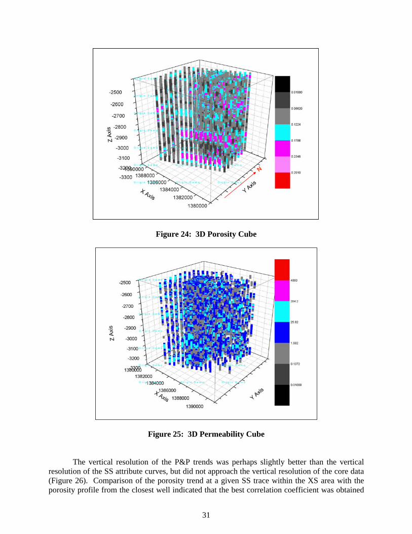
Estimated porosity and permeability (P&P) profiles were generated over this ~ 350 foot

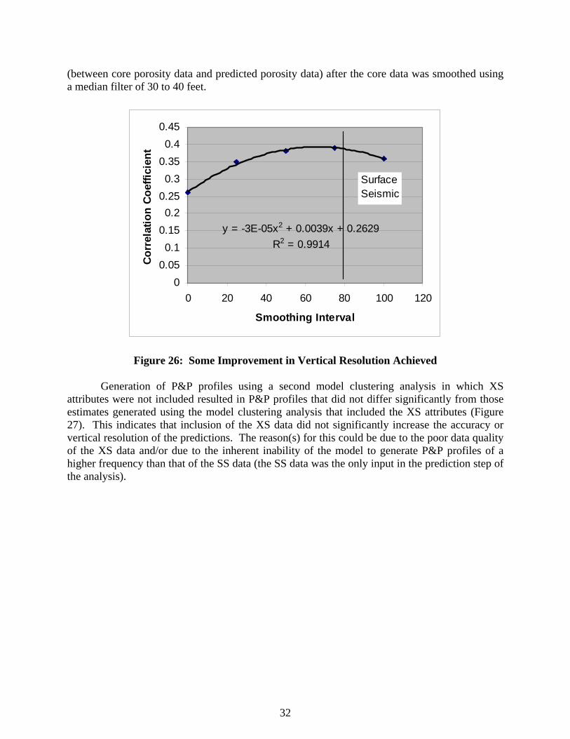
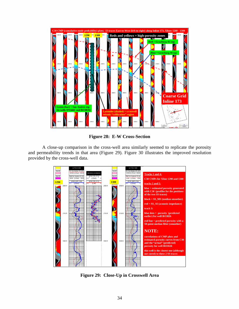
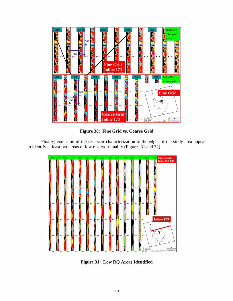
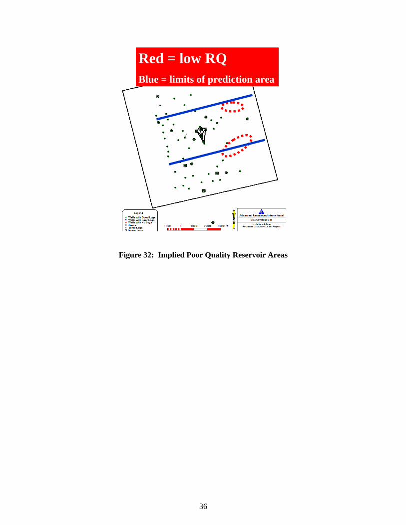
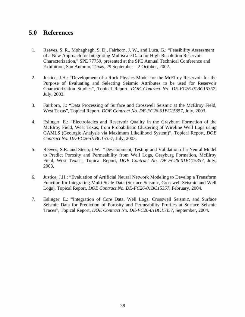
interval for SS traces within a coarse grid and a fine grid centered across the XS area in the middle of the overall study area (Figures 23 – 25). The P&P profiles generally showed the same trend of P&P exhibited by the core data. The dense spacing of the profiles permitted a detailed visualization of the geometry of high-reservoir quality zones (high P&P zones). In particular, there were two areas (one to the NE and one to the SE) where low-quality reservoir rocks were predicted throughout the 350 foot interval.

Figure 23: Inline/Crossline Scheme

1205 1210 1220 1230 1240 1250 1260 1340 1350 1360 1370 1380

Cross Lines

255

250

240

230

220

210

80

90

100

110

120

130

140

In Lines

LayOut of InLines and CrossLines Grid (176 inlines and 176 crosslines)

Notes: NOT TO SCALE; top inline and left crossline in grid are not at 10-line interval

Inline 170

Cro

sslin

e 12

90

Fine Grid

Coarse Grid

Crosswell seismic area (approximate location)

Fine: 150-182; 1280-1310; every other trace

Coarse: 143-203; 1240-1380; every 4th trace

1205 1210 1220 1230 1240 1250 1260 1340 1350 1360 1370 1380

Cross Lines

255

250

240

230

220

210

80

90

100

110

120

130

140

In Lines

LayOut of InLines and CrossLines Grid (176 inlines and 176 crosslines)

Notes: NOT TO SCALE; top inline and left crossline in grid are not at 10-line interval

Inline 170

Cro

sslin

e 12

90

Fine Grid

Coarse Grid

Crosswell seismic area (approximate location)

Fine: 150-182; 1280-1310; every other trace

Coarse: 143-203; 1240-1380; every 4th trace

31

Figure 24: 3D Porosity Cube

Figure 25: 3D Permeability Cube

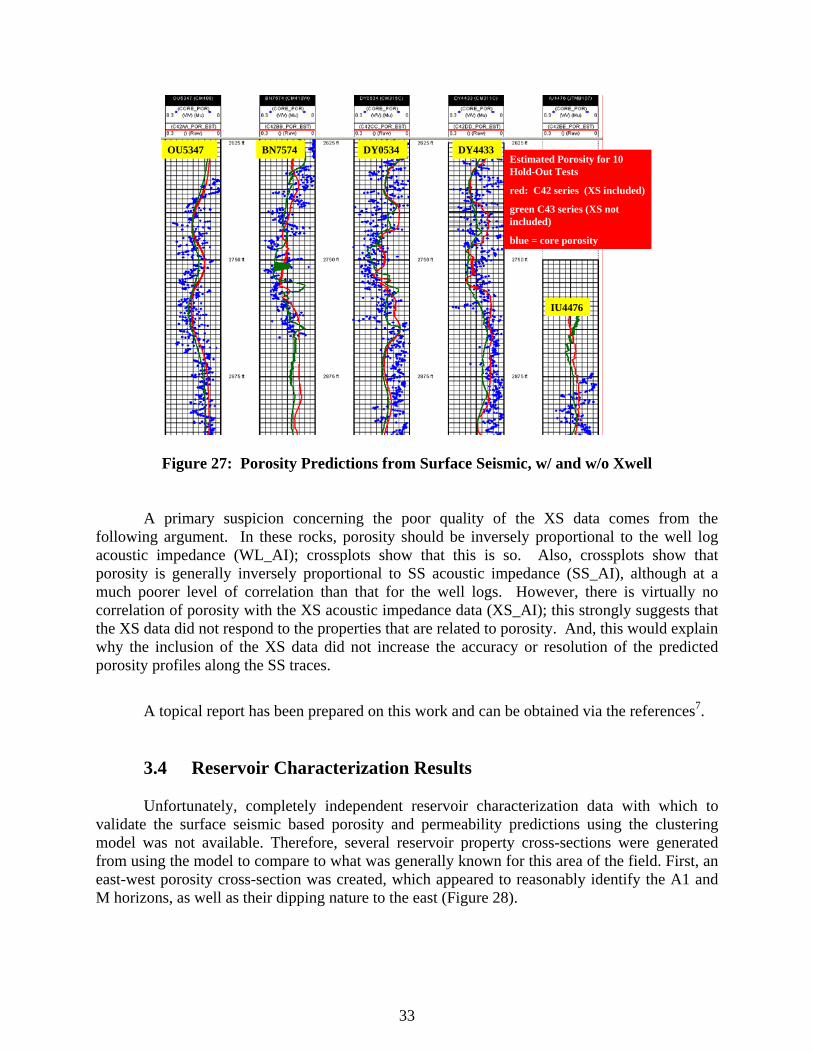
The vertical resolution of the P&P trends was perhaps slightly better than the vertical

resolution of the SS attribute curves, but did not approach the vertical resolution of the core data (Figure 26). Comparison of the porosity trend at a given SS trace within the XS area with the porosity profile from the closest well indicated that the best correlation coefficient was obtained

NN

32

(between core porosity data and predicted porosity data) after the core data was smoothed using a median filter of 30 to 40 feet.

Figure 26: Some Improvement in Vertical Resolution Achieved

Generation of P&P profiles using a second model clustering analysis in which XS

attributes were not included resulted in P&P profiles that did not differ significantly from those estimates generated using the model clustering analysis that included the XS attributes (Figure 27). This indicates that inclusion of the XS data did not significantly increase the accuracy or vertical resolution of the predictions. The reason(s) for this could be due to the poor data quality of the XS data and/or due to the inherent inability of the model to generate P&P profiles of a higher frequency than that of the SS data (the SS data was the only input in the prediction step of the analysis).

y = -3E-05x2 + 0.0039x + 0.2629R2 = 0.9914

00.050.1

0.150.2

0.250.3

0.350.4

0.45

0 20 40 60 80 100 120

Smoothing Interval

Corr

elat

ion

Coef

ficie

nt

SurfaceSeismic

33

Figure 27: Porosity Predictions from Surface Seismic, w/ and w/o Xwell

A primary suspicion concerning the poor quality of the XS data comes from the

following argument. In these rocks, porosity should be inversely proportional to the well log acoustic impedance (WL_AI); crossplots show that this is so. Also, crossplots show that porosity is generally inversely proportional to SS acoustic impedance (SS_AI), although at a much poorer level of correlation than that for the well logs. However, there is virtually no correlation of porosity with the XS acoustic impedance data (XS_AI); this strongly suggests that the XS data did not respond to the properties that are related to porosity. And, this would explain why the inclusion of the XS data did not increase the accuracy or resolution of the predicted porosity profiles along the SS traces.


3.4 Reservoir Characterization Results Unfortunately, completely independent reservoir characterization data with which to

validate the surface seismic based porosity and permeability predictions using the clustering model was not available. Therefore, several reservoir property cross-sections were generated from using the model to compare to what was generally known for this area of the field. First, an east-west porosity cross-section was created, which appeared to reasonably identify the A1 and M horizons, as well as their dipping nature to the east (Figure 28).

Estimated Porosity for 10 Hold-Out Tests

red: C42 series (XS included)

green C43 series (XS not included)

blue = core porosity

OU5347 BN7574 DY0534 DY4433

IU4476





OU5347 BN7574 DY0534 DY4433

IU4476





OU5347 BN7574 DY0534 DY4433

IU4476

34

Figure 28: E-W Cross-Section

A close-up comparison in the cross-well area similarly seemed to replicate the porosity

and permeability trends in that area (Figure 29). Figure 30 illustrates the improved resolution provided by the cross-well data.

Figure 29: Close-Up in Crosswell Area

C30 CMP (cumulative mode probability) plots; 13 traces East-to-West (left-to-right) along Inline 173, Xlines 1260 - 1380

1290 1300

Red = Grayburg A1 top

Blue = Grayburg M top

Green (bar) = San Andres top (in wells DY4441 and BO3826) Lavender (shaded) = crosswell

seismic “calibration” region

Reds and yellows = high-porosity zones

Coarse Grid Inline 173

C30 CMP (cumulative mode probability) plots; 13 traces East-to-West (left-to-right) along Inline 173, Xlines 1260 - 1380

1290 1300

Red = Grayburg A1 top

Blue = Grayburg M top

Green (bar) = San Andres top (in wells DY4441 and BO3826) Lavender (shaded) = crosswell

seismic “calibration” region

Reds and yellows = high-porosity zones


1290 1300

Tracks 1 and 4:

C30 CMPs for Xline 1290 and 1300

tracks 2 and 5:

blue = estimated porosity generated with C30 (profiles for the positions of the two SS traces)

black = SS_MS (median smoother)

red = SS_AI (acoustic impedance)

track 3:

blue dots = porosity (predicted earlier) for well BO3826

red line = predicted porosity with a 50-point median filter (smoother)

NOTE:correlations of CMP plots and estimated porosity curves from C30 and the “actual” (predicted) porosity for well BO3826

this well is the closest one (although not cored) to these 2 SS traces

1290 1300

Tracks 1 and 4:

C30 CMPs for Xline 1290 and 1300

tracks 2 and 5:

blue = estimated porosity generated with C30 (profiles for the positions of the two SS traces)

black = SS_MS (median smoother)

red = SS_AI (acoustic impedance)

track 3:

blue dots = porosity (predicted earlier) for well BO3826

red line = predicted porosity with a 50-point median filter (smoother)

NOTE:correlations of CMP plots and estimated porosity curves from C30 and the “actual” (predicted) porosity for well BO3826

this well is the closest one (although not cored) to these 2 SS traces

35

Figure 30: Fine Grid vs. Coarse Grid

Finally, extension of the reservoir characterization to the edges of the study area appear

to identify at least two areas of low reservoir quality (Figures 31 and 32).

Figure 31: Low RQ Areas Identified

1260 1280 1300 1320 1340 1360

1280 1284 1286 1290 1292 Inline 170

“fine grid”

C41b

Inline 173

“coarse grid”

C30

550 ft

110 ft

500 ft

500 ft

Fine Grid Inline 173

Fine Grid


1260 1280 1300 1320 1340 1360

1280 1284 1286 1290 1292 Inline 170

“fine grid”

C41b

Inline 173

“coarse grid”

C30

550 ft

110 ft

500 ft

500 ft

Fine Grid Inline 173

Fine Grid


1240 1250 1260 1270 1280 1290 1300 1310 1320 1330 1340 1350 1360 1370 1380 Coarse Grid, Inline 193, C44

Inline 193

1240 1250 1260 1270 1280 1290 1300 1310 1320 1330 1340 1350 1360 1370 1380 Coarse Grid, Inline 193, C44

Inline 193

36

Figure 32: Implied Poor Quality Reservoir Areas

Red = low RQBlue = limits of prediction area

Red = low RQBlue = limits of prediction area

37

4.0 Conclusions Based on the results from the project, the following conclusions have been drawn:








38

5.0 References

1. Reeves, S. R., Mohaghegh, S. D., Fairborn, J. W., and Luca, G.: “Feasibility Assessment of a New Approach for Integrating Multiscale Data for High-Resolution Reservoir Characterization,” SPE 77759, presented at the SPE Annual Technical Conference and Exhibition, San Antonio, Texas, 29 September – 2 October, 2002.

2. Justice, J.H.: “Development of a Rock Physics Model for the McElroy Reservoir for the

Purpose of Evaluating and Selecting Seismic Attributes to be used for Reservoir Characterization Studies”, Topical Report, DOE Contract No. DE-FC26-01BC15357, July, 2003.

3. Fairborn, J.: “Data Processing of Surface and Crosswell Seismic at the McElroy Field,

West Texas”, Topical Report, DOE Contract No. DE-FC26-01BC15357, July, 2003.

4. Eslinger, E.: “Electrofacies and Reservoir Quality in the Grayburn Formation of the McElroy Field, West Texas, from Probabilistic Clustering of Wireline Well Logs using GAMLS (Geologic Analysis via Maximum Likelihood System)”, Topical Report, DOE Contract No. DE-FC26-01BC15357, July, 2003.

5. Reeves, S.R. and Steen, J.W.: “Development, Testing and Validation of a Neural Model

to Predict Porosity and Permeability from Well Logs, Grayburg Formation, McElroy Field, West Texas”, Topical Report, DOE Contract No. DE-FC26-01BC15357, July, 2003.

6. Justice, J.H.: “Evaluation of Artificial Neural Network Modeling to Develop a Transform

Function for Integrating Multi-Scale Data (Surface Seismic, Crosswell Seismic and Well Logs), Topical Report, DOE Contract No. DE-FC26-01BC15357, February, 2004.

7. Eslinger, E.: “Integration of Core Data, Well Logs, Crosswell Seismic, and Surface

Seismic Data for Prediction of Porosity and Permeability Profiles at Surface Seismic Traces”, Topical Report, DOE Contract No. DE-FC26-01BC15357, September, 2004.

Date post:	03-Apr-2018
Category:	Documents
Upload:	dangkien
View:	216 times
Download:	2 times

Development of an Advanced Approach for Next-Generation ... of an Advanced Approach for Next... ·...

Documents