Development of an Empirically-Based

research for safer communities

URBAN INSTITUTE Justice Policy Center

Development of an Empirically-Based Risk Assessment Instrument FINAL REPORT

Prepared for: DC Pretrial Services Agency Laura Winterfield Mark Coggeshall Adele Harrell

RE

SE

AR

CH

R

EP

OR

T

April 2003

URBAN INSTITUTE Justice Policy Center 2100 M STREET, NW WASHINGTON, DC 20037 www.urban.org

The views expressed are those of the authors, and should not be attributed to The Urban Institute, its trustees, or its fun-ders.

Contents

Chapter 1. Overview........................................................................ 1 PURPOSE OF STUDY................................................................................................................................1 SUMMARY FINDINGS ON INSTRUMENT ...........................................................................................................2 ORGANIZATION OF THE REPORT .................................................................................................................2

Chapter 2. Research Questions and Methods ........................................... 3 RESEARCH QUESTIONS.............................................................................................................................3 THE SAMPLE ........................................................................................................................................4 THE DATA ...........................................................................................................................................4 SAMPLE CHARACTERISTICS........................................................................................................................5 INSTRUMENT CONSTRUCTION METHODS ........................................................................................................6

Step 1. Refining and Expanding Predictor Measures .........................................................................................6 Step 2. Selecting Predictors for the Instrument..............................................................................................7 Step 3. Developing Instrument Scores .........................................................................................................7 Step 4. Developing Supervision Level Classification .........................................................................................7

ASSESSING MODEL PERFORMANCE ...............................................................................................................9 Overall Performance..............................................................................................................................9 Performance at Alternative Various Cut-points ..............................................................................................9 Base Rate Dispersion Analysis ................................................................................................................. 10

ASSESSING EXTERNAL VALIDITY OF THE MODEL RESULTS: COMPARISON OF STATISTICAL AND CLINICAL RISK CLASSIFICATION... 10 ASSESSING MODEL APPLICABILITY TO FEDERAL DEFENDANTS AND DETAINEES........................................................... 11

Chapter 3. Instrument Construction .................................................... 12 SELECTION OF PREDICTORS FOR THE INSTRUMENT ......................................................................................... 12 INSTRUMENT SCORES ............................................................................................................................ 14 THE INSTRUMENT ................................................................................................................................ 17

Chapter 4. Instrument Performance .................................................... 19 THE DISTRIBUTION OF RISK ..................................................................................................................... 19 ASSESSING MODEL PERFORMANCE ............................................................................................................. 21

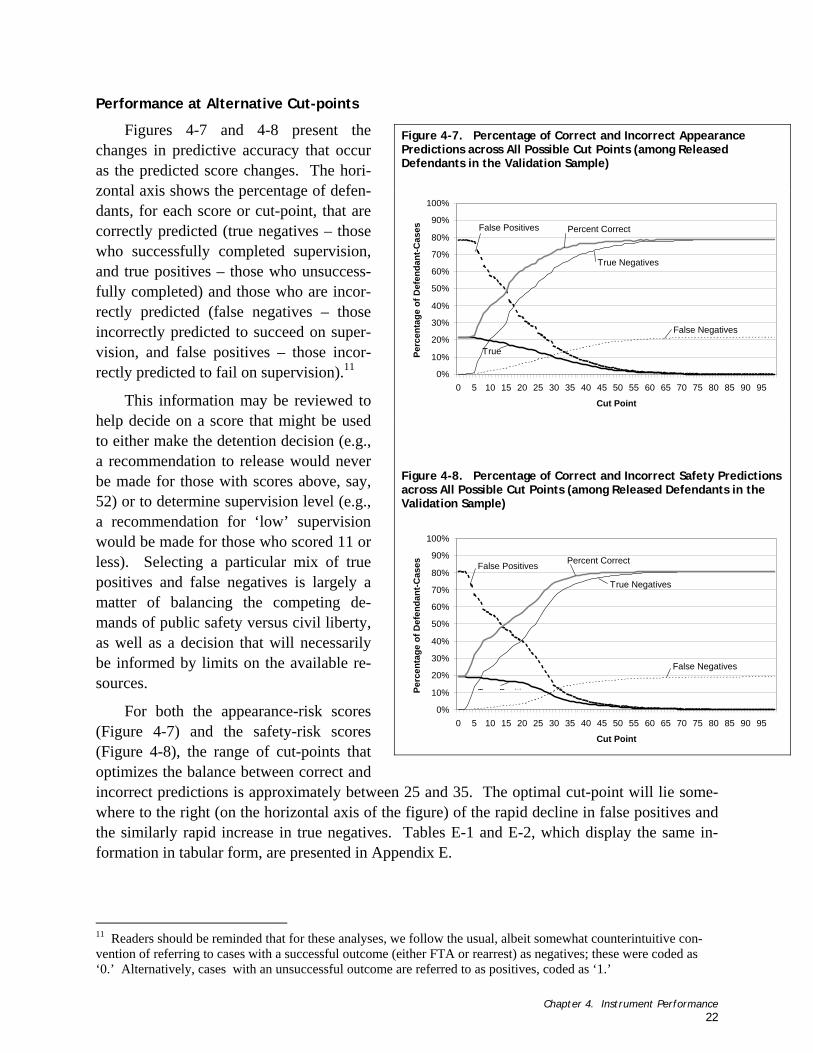
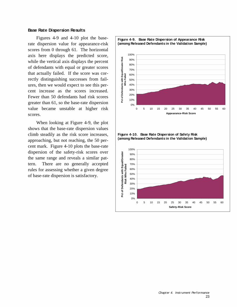
Overall Performance............................................................................................................................ 21 Performance at Alternative Cut-points ...................................................................................................... 22 Base Rate Dispersion Results .................................................................................................................. 23

ASSESSING EXTERNAL VALIDITY OF THE MODEL RESULTS: COMPARISON OF STATISTICAL AND CLINICAL RISK CLASSIFICATION.. 24 ASSESSING MODEL APPLICABILITY FOR FEDERAL DEFENDANTS AND DETAINEES ......................................................... 25

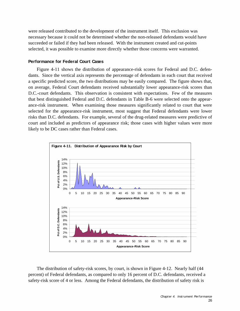
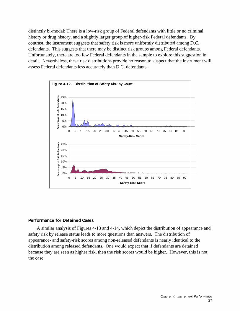
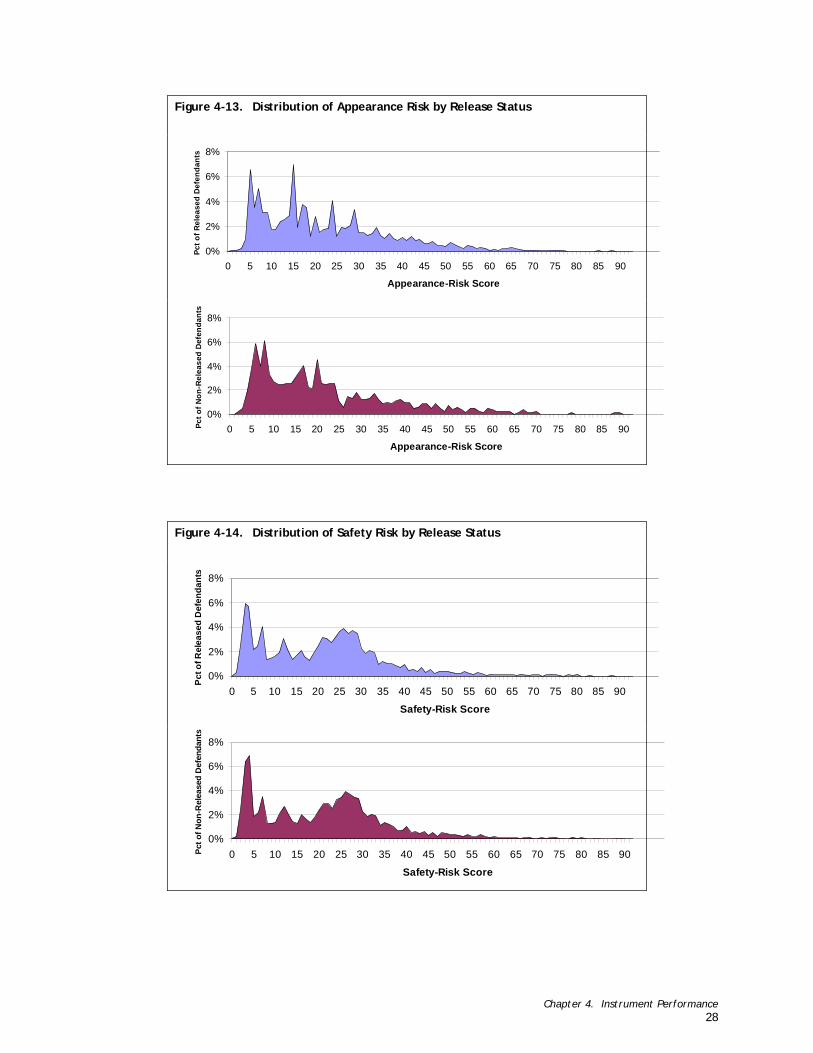
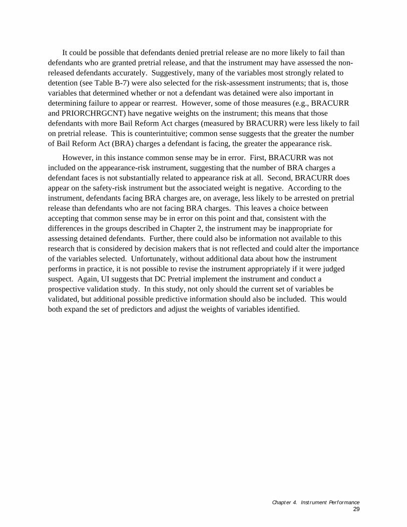
Performance for Federal Court Cases........................................................................................................ 26 Performance for Detained Cases.............................................................................................................. 27

Chapter 5. Summary and Recommendations ........................................... 30 THE INSTRUMENT ................................................................................................................................ 30 USING THE SPREADSHEET ....................................................................................................................... 31 SPECIAL CONSIDERATIONS AND LIMITATIONS................................................................................................. 32 RECOMMENDATIONS FOR USE AND FUTURE DEVELOPMENT ................................................................................ 33

Using The Instrument ........................................................................................................................... 33 Ongoing Validation .............................................................................................................................. 34

Appendix A. Data Processing ............................................................. 36 INITIAL DATA PROCESSING...................................................................................................................... 36

Contents ii

SELECTION OF SAMPLE DEFENDANT-CASES ................................................................................................... 39 Overview.......................................................................................................................................... 39 Detail on the Identification of Sample Defendants ........................................................................................ 40

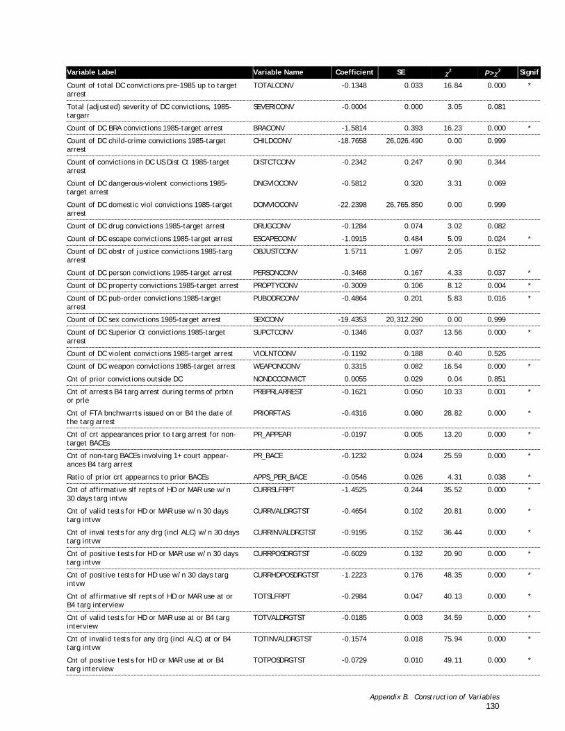
Appendix B. Construction of Variables ................................................. 42 ASSEMBLY OF ANALYSIS FILE ................................................................................................................... 42 VARIABLE DEFINITION ........................................................................................................................... 43 SAMPLE CHARACTERISTICS...................................................................................................................... 47

Appendix C. Statistical Models ......................................................... 137 CHAID PARAMETERS.............................................................................................................................137

Terminal Nodes from CHAID Model of FTA ................................................................................................. 138 Terminal Nodes from CHAID Model of Arrest............................................................................................... 139

LOGISTIC REGESSION RESULTS ................................................................................................................139 COMPUTATION OF RISK SCORES...............................................................................................................142

Appendix D. Assessing Model Performance ........................................... 143 METHODS.........................................................................................................................................143

Classification Table Analysis.................................................................................................................. 143 Receiver-Operator Curve Analysis ........................................................................................................... 144

RESULTS..........................................................................................................................................145 Classification Table Results................................................................................................................... 145 Receiver-Operator Curve Results ............................................................................................................ 146

Appendix E. Supporting Tables......................................................... 147

References ................................................................................ 149

Contents iii

Tables

Chapter 3. Instrument Construction .................................................... 14 Table 3-1. Predictor Measures of Each Outcome Selected by Stepwise Logistic Regression ......................................... 13

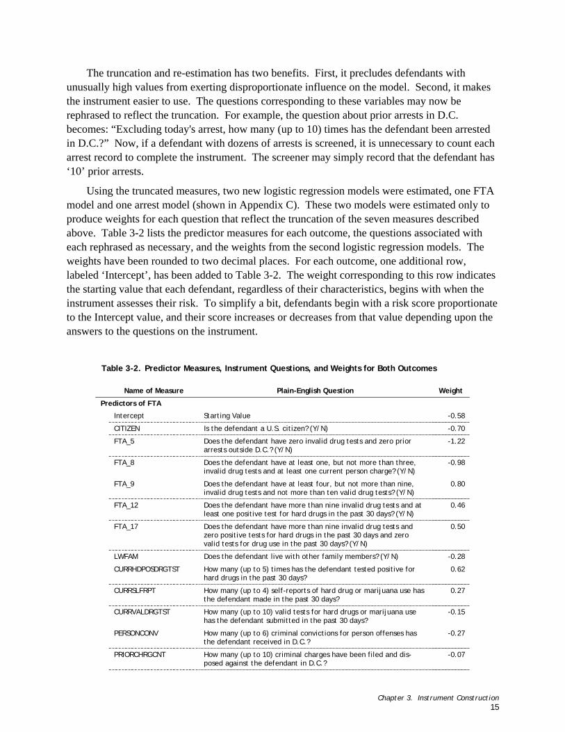
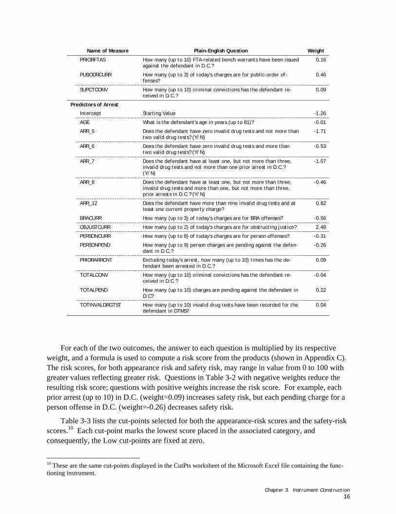
Table 3-2. Predictor Measures, Instrument Questions, and Weights for Both Outcomes ............................................. 15

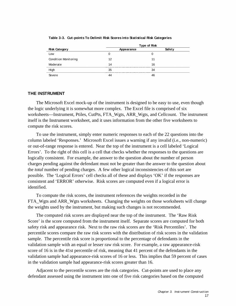
Table 3-3. Cut-points To Delimit Risk Scores into Statistical Risk Categories .......................................................... 17

Chapter 4. Instrument Performance .................................................... 21 Table 4-1. Appearance Risk: A Comparison of Statistical and Clinical Risk Categories ............................................... 24

Table 4-2. Safety Risk: A Comparison of Statistical and Clinical Risk Categories ...................................................... 25

Appendix B. Construction of Variables ................................................. 42 Table B-1. All Sample Defendants: Comparison and Summary of D.C. PSA

Draft Instruments and Variables Constructed by Urban Institute Staff ..................................................... 48

Table B-2. Sample Defendants in U.S. District Court: Comparison of D.C. PSA Draft Instruments and Variables Constructed by Urban Institute Staff ..................................................... 64

Table B-3. Sample Defendants in D.C. Superior Court: Comparison of D.C. PSA Draft Instruments and Variables Constructed by Urban Institute Staff ..................................................... 80

Table B-4. Sample Defendants Granted Pre-Trial Release: Comparison of D.C. PSA Draft Instruments and Variables Constructed by Urban Institute Staff ..................................................... 96

Table B-5. Sample Defendants Denied Pre-Trial Release: Comparison of D.C. PSA Draft Instruments and Variables Constructed by Urban Institute Staff .................................................... 112

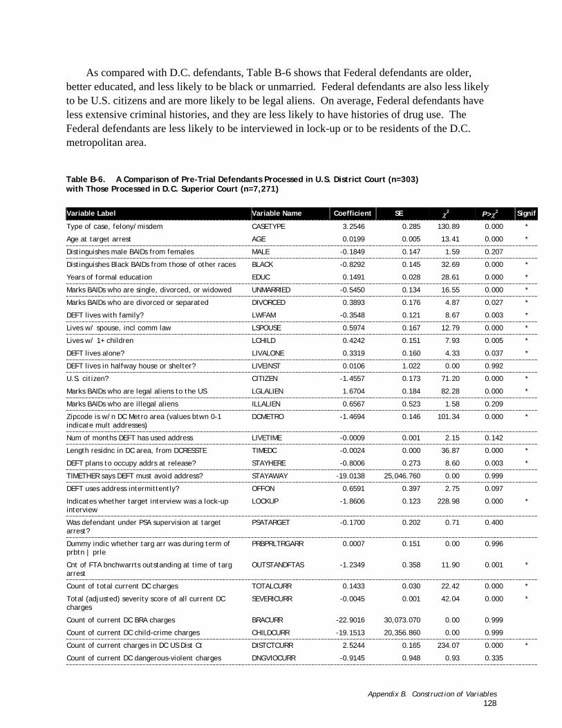
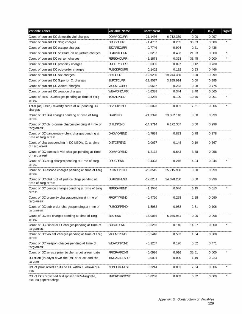
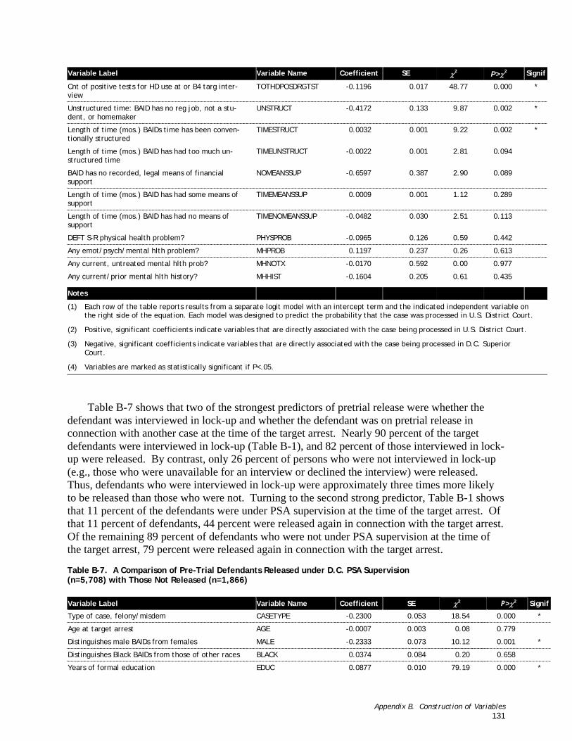
Table B-6. A Comparison of Pre-Trial Defendants Processed in U.S. District Court (n=303) with Those Processed in D.C. Superior Court (n=7,271)............................................................................ 128

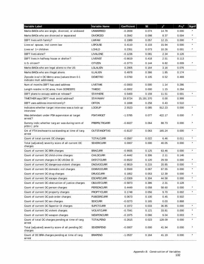
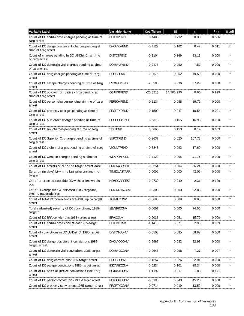
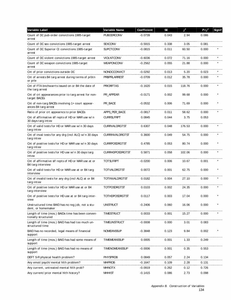
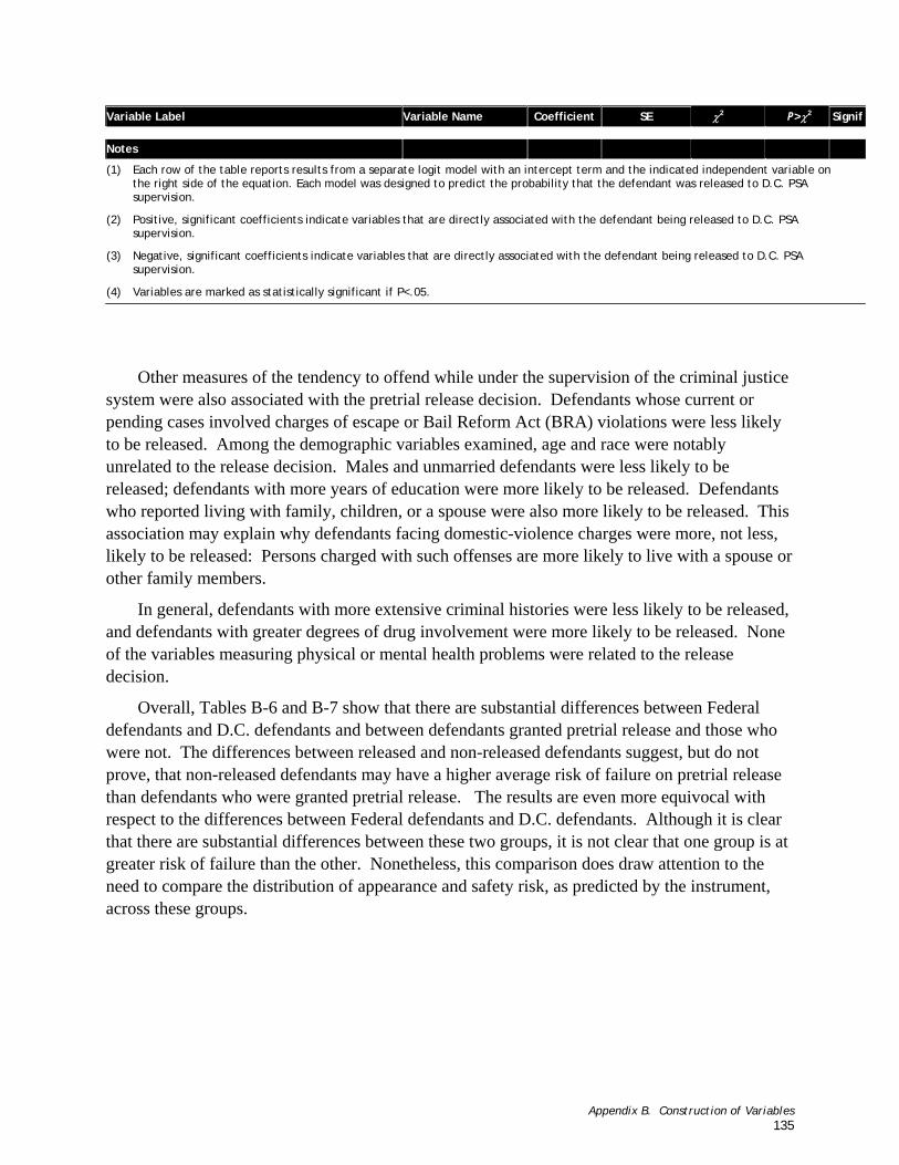
Table B-7. A Comparison of Pre-Trial Defendants Released under D.C. PSA Supervision (n=5,708 with Those Not Released (n=1,866) ............................................................................................ 132

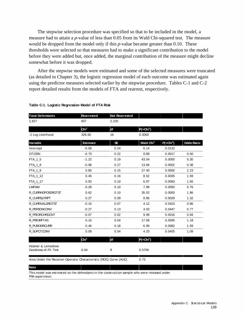
Appendix C. Statistical Models ......................................................... 137 Table C-1. Logistic Regression Model of FTA Risk ..........................................................................................140

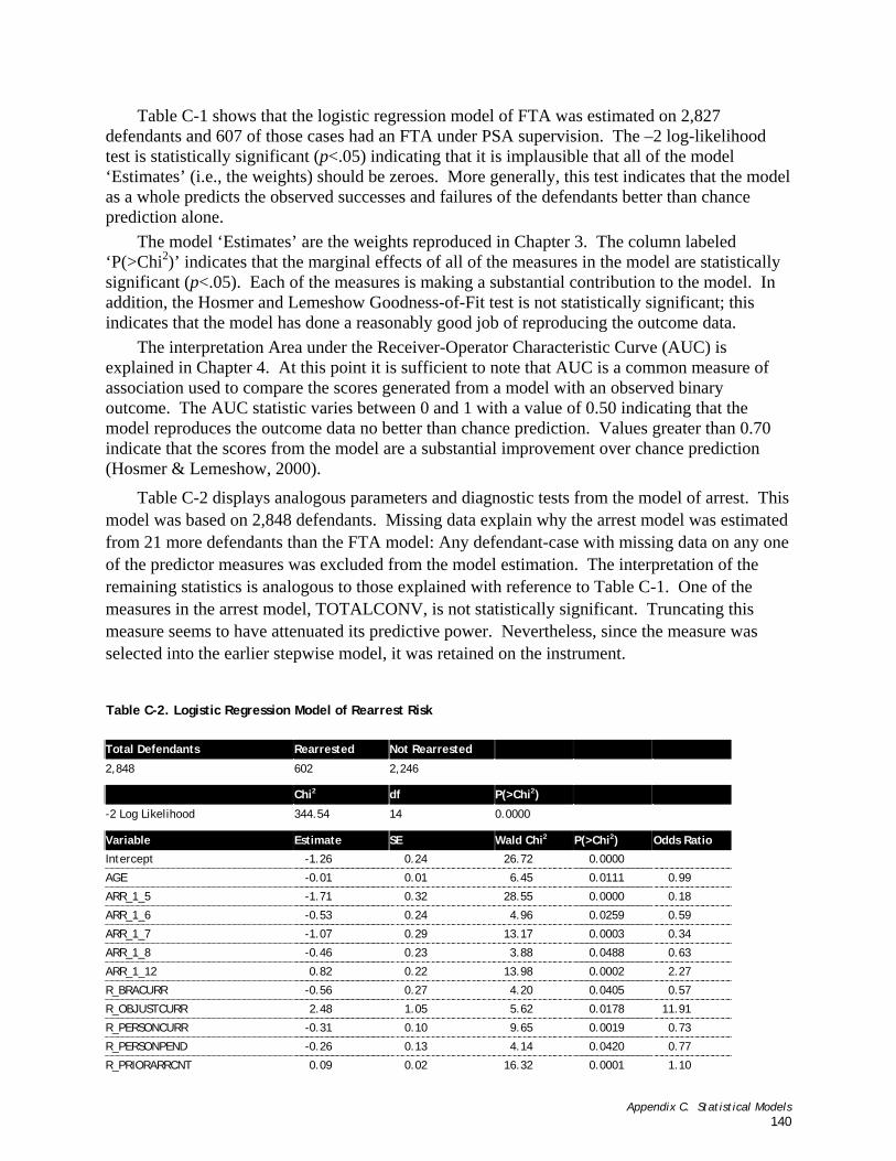
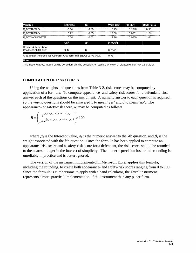
Table C-2. Logistic Regression Model of Rearrest Risk.....................................................................................141

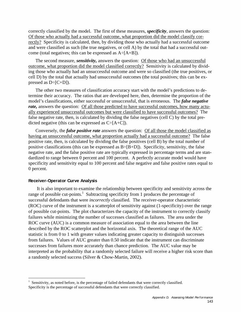
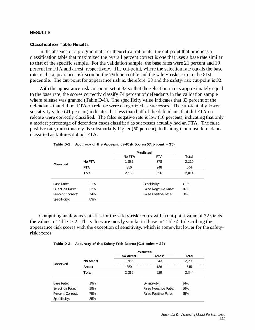
Appendix D. Assessing Model Performance ........................................... 143 Table D-1. Accuracy of the Appearance-Risk Scores (Cut-point = 33)...................................................................145

Table D-2. Accuracy of the Safety-Risk Scores (Cut-point = 32) .........................................................................145

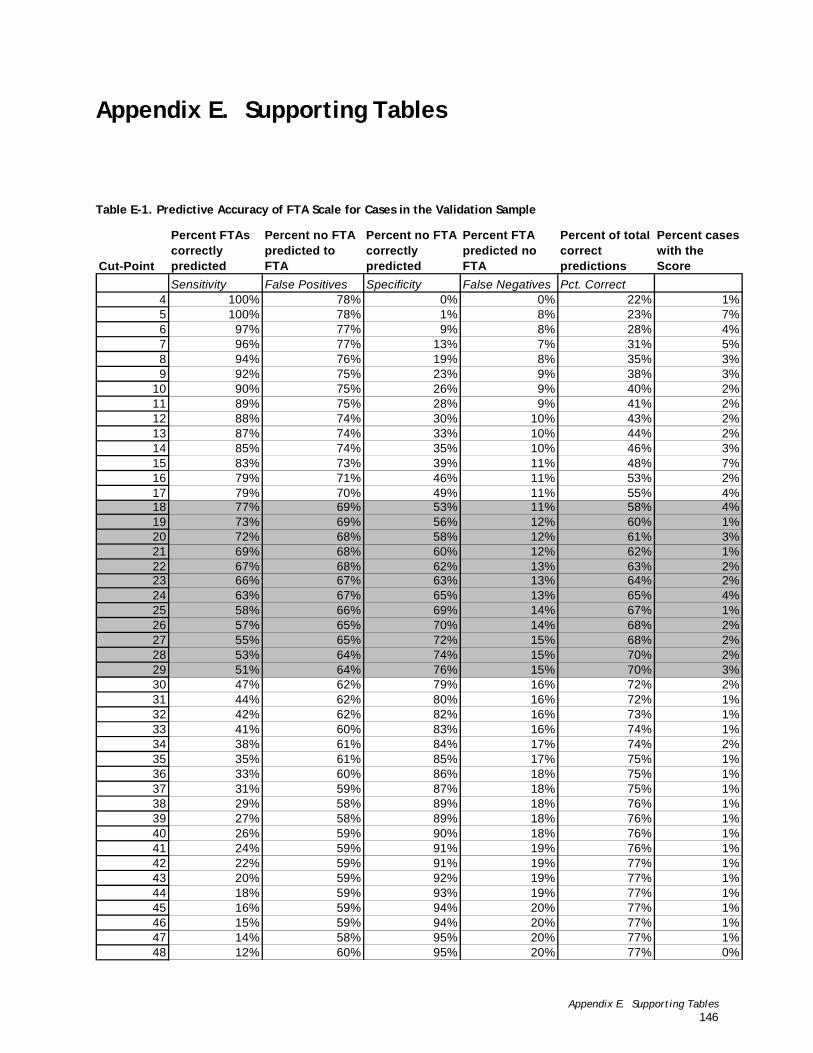
Appendix E. Supporting Tables......................................................... 147 Table E-1. Predictive Accuracy of FTA Scale for Cases in the Validation Sample .....................................................147

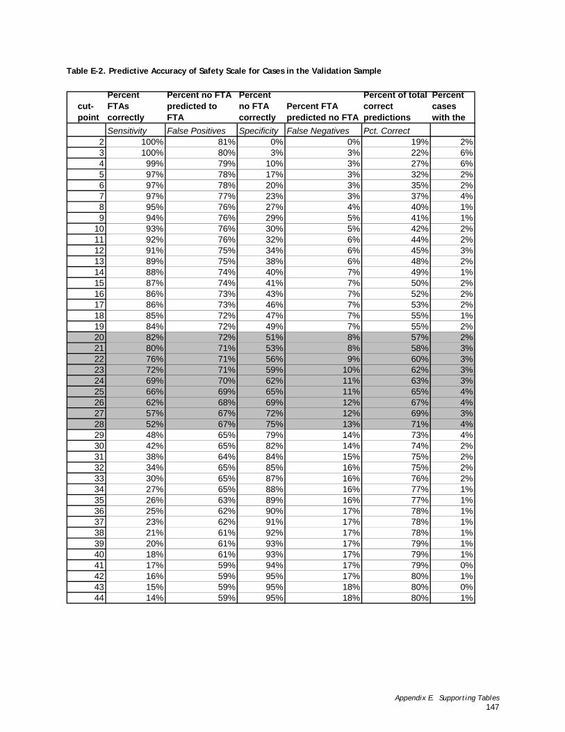
Table E-2. Predictive Accuracy of Safety Scale for Cases in the Validation Sample ..................................................148

Contents iv

Figures

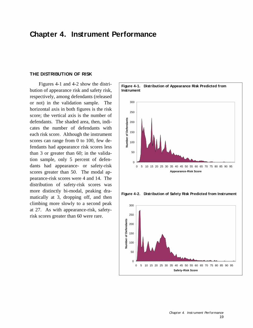
Chapter 4. Instrument Performance .................................................... 21 Figure 4-1. Distribution of Appearance Risk Predicted from Instrument ................................................................. 19

Figure 4-2. Distribution of Safety Risk Predicted from Instrument........................................................................ 19

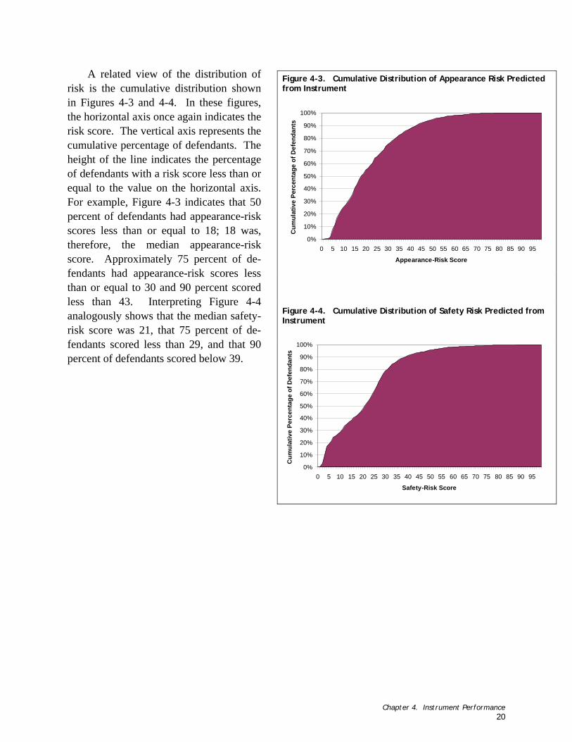
Figure 4-3. Cumulative Distribution of Appearance Risk Predicted from Instrument .................................................. 20

Figure 4-4. Cumulative Distribution of Safety Risk Predicted from Instrument ......................................................... 20

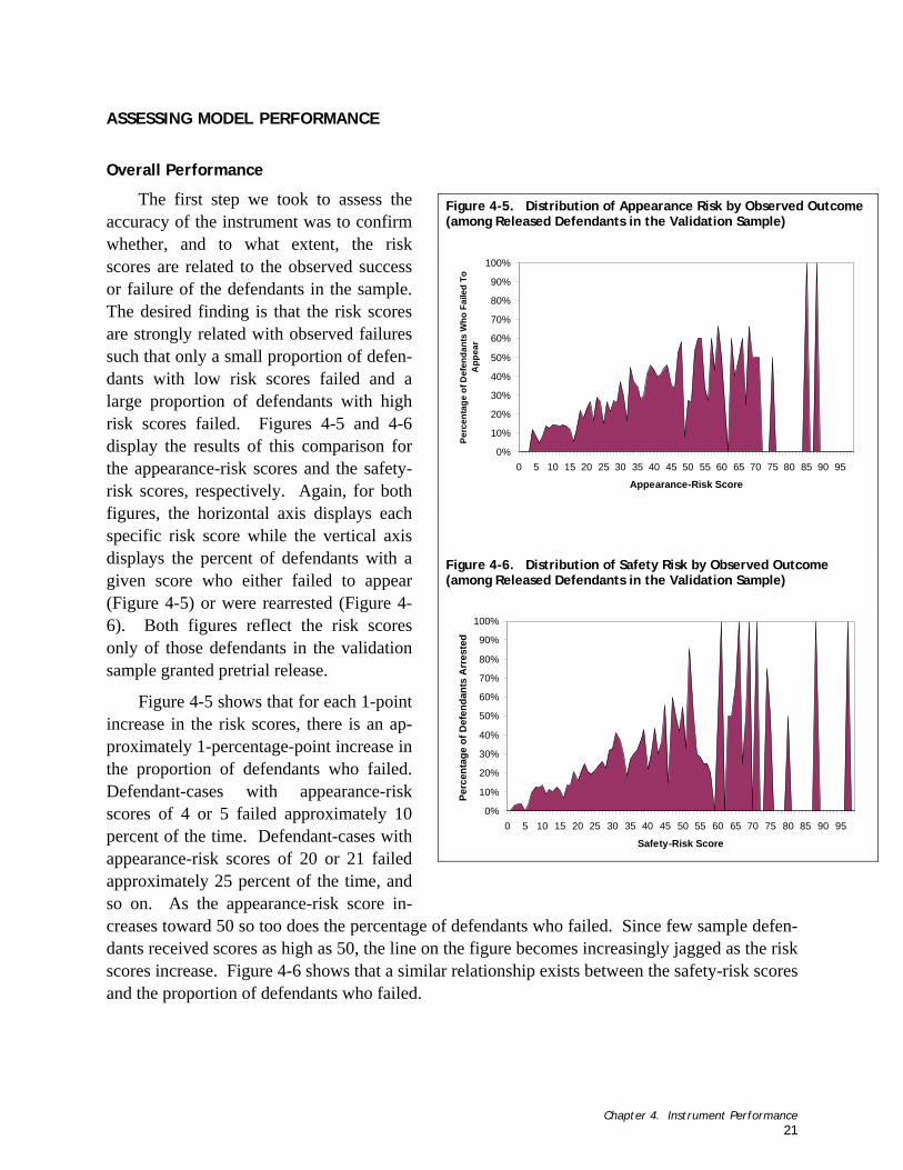
Figure 4-5. Distribution of Appearance Risk by Observed Outcome (among Released Defendants in the Validation Sample)...................................................................... 21

Figure 4-6. Distribution of Safety Risk by Observed Outcome (among Released Defendants in the Validation Sample)...................................................................... 21

Figure 4-7. Percentage of Correct and Incorrect Appearance Predictions across All Possible Cut Points (among Released Defendants in the Validation Sample)...................................................................... 22

Figure 4-8. Percentage of Correct and Incorrect Safety Predictions across All Possible Cut Points (among Released Defendants in the Validation Sample)...................................................................... 22

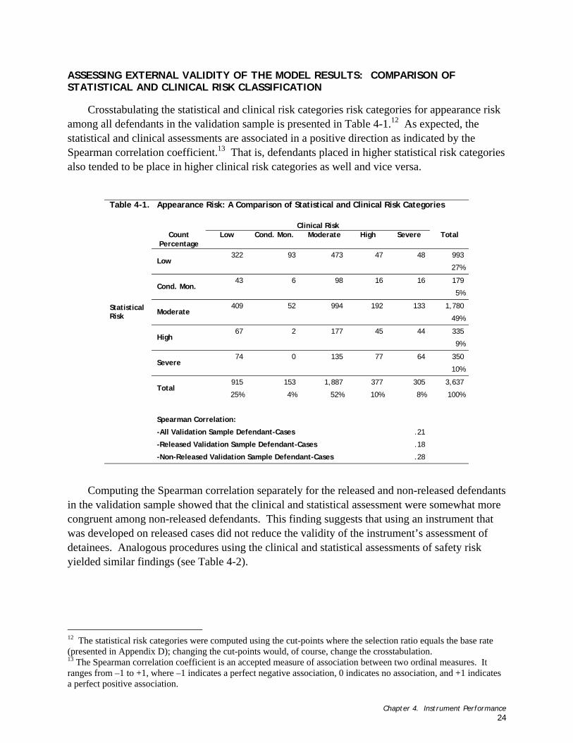
Figure 4-9. Base Rate Dispersion of Appearance Risk (among Released Defendants in the Validation Sample)...................................................................... 23

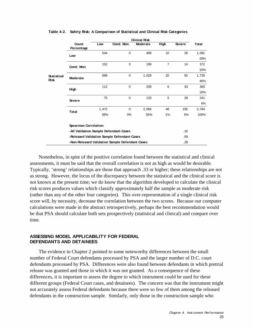
Figure 4-10. Base Rate Dispersion of Safety Risk (among Released Defendants in the Validation Sample)...................................................................... 23

Figure 4-11. Distribution of Appearance Risk by Court ....................................................................................... 26 Figure 4-12. Distribution of Safety Risk by Court.............................................................................................. 27 Figure 4-13. Distribution of Appearance Risk by Release Status ............................................................................ 28 Figure 4-14. Distribution of Safety Risk by Release Status................................................................................... 28

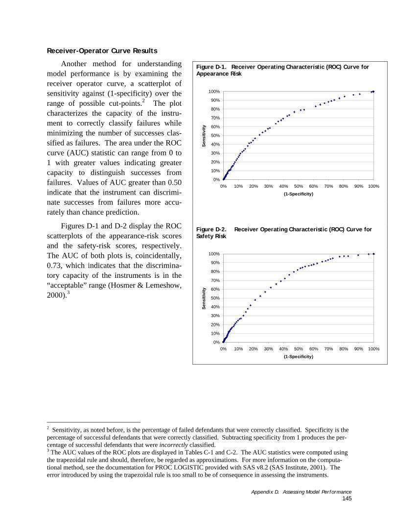
Appendix D. Assessing Model Performance ........................................... 143 Figure D-1. Receiver Operating Characteristic (ROC) Curve for Appearance Risk...................................................... 146

Figure D-2. Receiver Operating Characteristic (ROC) Curve for Safety Risk ............................................................ 146

Development of an Empirically-Based Risk Assessment Instrument – Summary 1

Overview

PURPOSE OF STUDY

In 2001, the Urban Institute was commissioned by the District of Columbia Pretrial Services Agency (PSA) to develop a risk assessment instrument to assist its diagnosticians in recommending conditions of pretrial release for the thousands of defendants they process each year. This is the final report on the second and final phase of the instrument development. This phase of the research built on the earlier work by extending the period for observing outcomes by 14 months (from nearly two years to three years or longer), expanding the set of predictor items considered for inclusion on the instrument, and searching for combinations of items for inclusion.

The resulting instrument is intended to serve two primary goals. The first goal is to make the development of release recommendations more objective and consistent across defendants. The attainment of this goal should improve the transparency of PSA assessment and recommendation processes to observers both inside and outside the agency. The second goal is to improve the accuracy of decision-making based on risk assessment. Improved accuracy should increase public safety, reduce court costs associated with non-appearance, and reduce the number of low-risk defendants whose liberty is restricted.

The instrument is designed to predict two outcomes, risk of failure-to-appear, or FTA (indicated by issuance of a bench warrant for failure-to-appear), and risk of rearrest (which included either a new arrest record or a citation). Measures that might predict either or both of these two outcomes (i.e., FTA or arrest under supervision) were created from the Automated Bail Agency Data Base (ABADABA) and Drug Testing Management System (DTMS) data. The data included information about the criminal histories, demographics, health, employment, and drug use of all defendants processed by PSA during the study period.

Candidate predictors were constructed from these data. They included items on a list provided by PSA, based on institutional understanding of the characteristics of defendants who fail, and items suggested by UI, based on knowledge of the research literature on the prediction of criminal outcomes. The list was constrained, however, to data in the existing ABADABA and DTMS; some candidate predictors could not be measured with available information. The significant predictors of either outcome (FTA or rearrest) are included in the final instrument.

The assessment instrument was developed using data on a cohort of defendants processed by PSA between January 1, 1999 and June 30, 1999. This time period was selected jointly with PSA because it was: 1) sufficiently recent that changes in the defendant population between 1999 and the present were expected to be of minor importance to the form and function of the instrument, but also 2) sufficiently long ago that nearly all of the defendants would have completed their PSA supervision before the data were provided to UI for analysis.

The scores on the instrument range from 0 to 100 for each risk outcome. The instrument scoring is designed to assist PSA diagnosticians in prospectively assessing the appearance and safety risk posed by individual defendants. Once a diagnostician has answered all of the questions on the instrument, the instrument weights the answers to compute two risk scores (one


each for appearance risk and for safety risk) that range from 0 to 100.1 These scores are then used to classify the level of risk into five categories that could be used when making a release recommendation for court in the bail report. The risk score and risk category could be included in the bail report as well to provide the judge with the benefit of this information.

SUMMARY FINDINGS ON INSTRUMENT

UI is submitting the instrument in the form of a Microsoft Excel spreadsheet that can be used to compute risk scores based on the answers to the questions input into the appropriate cells. Delivering the instrument as a functioning spreadsheet is the most concise, comprehensive explanation of how the questions, answers, and corresponding weights relate to each other to produce the risk scores. The spreadsheet allows PSA administrators to explore the consequences of adjusting the cut-point values used to assign one of five risk categories (i.e., Low, Condition Monitoring, Moderate, High, or Severe) to defendants based on the risk scores, which range from 0-100, computed by the instrument. The spreadsheet instrument may also be printed to hard copy, complete with instructions for answering each question.

1 Although the computation of the risk scores from the answers and weights is purely arithmetic, it is not simple. Even a user who felt competent to perform the computations would shortly find it tedious to perform them with a hand calculator. Ideally, the instrument should be integrated into the management information system used by PSA so that the computer can calculate the scores with little or no input from the user.


USING THE SPREADSHEET

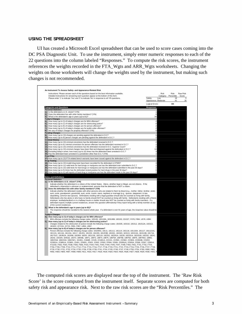
UI has created a Microsoft Excel spreadsheet that can be used to score cases coming into the DC PSA Diagnostic Unit. To use the instrument, simply enter numeric responses to each of the 22 questions into the column labeled “Responses.” To compute the risk scores, the instrument references the weights recorded in the FTA_Wgts and ARR_Wgts worksheets. Changing the weights on those worksheets will change the weights used by the instrument, but making such changes is not recommended.

The computed risk scores are displayed near the top of the instrument. The ‘Raw Risk

Score’ is the score computed from the instrument itself. Separate scores are computed for both safety risk and appearance risk. Next to the raw risk scores are the “Risk Percentiles.” The

An Instrument To Assess Safety- and Appearance-Related Risk

Instructions: Please answer each of the questions based on the best information available. Risk Risk Raw RiskDetailed instructions for answering each question appear at the bottom of this form. Category Percentile ScorePlease enter '1' to indicate 'Yes' and '0' to indicate 'No' in response to all Y/N questions. Safety Low 18 5

Appearance Moderate 41 16

Logical Errors: OK

Categories and Questions Responses Outcome Appearanc SafetyPersonal Statistics -0.58 -1.261.) Is the defendant a U.S. citizen? (Y/N) 1 1 -0.72.) Does the defendant live with other family members? (Y/N) 0 1 03.) What is the defendant's age in years (up to 81)? 34 2 -0.34Today's Charges 0 04.) How many (up to 3) of today's charges are for BRA offenses? 2 2 -1.125.) How many (up to 2) of today's charges are for obstructing justice? 0 2 06.) How many (up to 8) of today's charges are for person offenses? 2 3 -0.627.) How many (up to 3) of today's charges are for public-order offenses? 2 1 0.928.) Are any of today's charges for property offenses? (Y/N) 0 2Pending Charges -0.98 09.) How many (up to 10) charges are pending against the defendant in D.C? 5 2 1.110.) How many (up to 9) person charges are pending against the defendant in D.C.? 2 2 -0.52Criminal History 0 011.) How many (up to 10) criminal convictions has the defendant received in D.C.? 2 2 -0.0812.) How many (up to 6) criminal convictions for person offenses has the defendant received in D.C.? 1 1 -0.2713.) How many (up to 10) criminal convictions has the defendant received in D.C. Superior Court? 2 1 0.1814.) How many (up to 10) criminal charges have been filed and disposed against the defendant in D.C.? 10 1 -0.715.) Excluding today's arrest, how many (up to 10) times has the defendant been arrested in D.C.? 3 2 0.2716.) Has the defendant been arrested in a jurisdiction other than D.C.? (Y/N) 1 1Prior FTAs 0 -0.4617.) How many (up to 10) FTA-related bench warrants have been issued against the defendant in D.C.? 2 1 0.32Drug Testing 0 018.) How many (up to 10) invalid drug tests have been recorded for the defendant in DTMS? 3 3 0.1219.) How many (up to 11) valid tests for hard drugs or marijuana use has the defendant ever submitted in D.C.? 2 320.) How many (up to 10) valid tests for hard drugs or marijuana use has the defendant submitted in the past 30 days? 1 1 -0.1521.) How many (up to 5) times has the defendant tested positive for hard drugs in the past 30 days? 0 1 022.) How many (up to 4) self-reports of hard drug or marijuana use has the defendant made in the past 30 days? 1 1 0.27

0.156 0.052Notes and DefinitionsPersonal Statistics1.)

2.) Does the defendant live with other family members? (Y/N)

3.) What is the defendant's age in years (up to 81)?

Today's Charges4.) How many (up to 3) of today's charges are for BRA offenses?

5.) How many (up to 2) of today's charges are for obstructing justice?

6.) How many (up to 8) of today's charges are for person offenses?

BRA offenses include the following charge codes: 183146, 183146A, 183146B, 183150, 231327, F078, F994, U078, U994.

Charges related to the obstruction of justice include the following charge codes: 181505, 181510, 181512, 181512A, 181513, 181622, 22722A, 22723, F855, F967, U855, U967.

Person offenses include the following charge codes: 161005G, 18111, 181111, 181114, 181116, 181116A, 181117, 181121A1, 18112A, 18113A, 18115A, 18117, 181201, 181202, 181203, 181203B, 181501, 181503, 181513, 181513A, 181513B, 181716, 181751C, 181952A, 181958, 181959, 18203, 182113E, 182119, 182252, 182261A, 18228, 182331A, 182331B, 182332, 18241, 18242, 183184, 18351E, 18373, 18844E, 18871, 18872, 18873, 18875, 18875A, 18875B, 18875D, 18876, 18879A2, 18892, 18922G8, 18922G9, 18922W1, 191951, 21848E, 22105, 221801A, 222101, 222901, 222902, 222903, 222903B, 223202, 223501A, 223851A, 223901, 22401, 225001, 22501, 22502, 22503, 22504, 22505, 22505(A), 22505A, 22506, 22507, 22901A, 47223D, F002, F003, F038, F055, F056, F433, F434, F441, F443, F444, F445, F447, F448, F450, F451, F701, F702, F703, F704, F705, F709, F710, F711, F712, F714, F715, F716, F717, F718, F720, F721, F722, F723, F724, F725, F726, F727, F728, F729, F730, F731, F732, F734, F735, F736, F738, F739, F741, F744, F745, F746, F747, F749, F750, F754, F760, F800, F801, F802, F803, F805, F807, F808, F809, F811, F816, F817, F818, F819, F820, F824, F825, F826, F827, F828, F829, F830, F831, F

Is the defendant a U.S. citizen? (Y/N)Indicate whether the defendant is a citizen of the United States. Aliens, whether legal or illegal, are not citizens. If the defendant's citizenship is unknown or undetermined, assume that the defendant is NOT a citizen.

Indicate whether the defendant resides with other persons who are related to them by blood (e.g., mother, father, brother, sister, aunt, uncle, grandparent, grandchild, aunt, uncle, cousin, niece, nephew) or marriage (e.g., spouse, stepparent, in-law, stepsibling, common-law spouse). Defendants residing with a legal guardian should also be counted as living with family. Defendants who live alone or who have no family should NOT be counted as living with family. Defendants residing with a friend, employer, landlady/landlord or in a halfway house or shelter should also NOT be counted as living with family members. If a defendant reports multiple current residences, answer this question affirmatively if they report living with a family member at any of the current residences.

The response should be rounded to the nearest whole year. If a defendant is over 81 years of age, the response value should be 81.


percentile scores compare the raw risk scores with the distribution of risk scores in the validation sample; the percentile risk score is proportional to the percentage of defendants in the validation sample with an equal or lesser raw risk score.

Adjacent to the percentile scores are the risk categories. Cut-points are used to place any defendant assessed using the instrument into one of five risk categories based on the computed raw risk scores. The risk categories range from “Low” to “Severe.” For each category there are two cut-points, one each for appearance risk and safety risk. Defendants with raw risk scores greater than or equal to the cut-point value (but less than the cut-point value of the next higher category) are placed in the associated risk category.

Summary and Recommendations

THE INSTRUMENT

The Risk Prediction Instrument is comprised of 22 items, making up two subscales: the Safety Risk Scale and the Appearance Risk Scale.

Items were selected for inclusion if they were significantly related to subsequent arrest or failure to appear at court hearings, based on analysis of a sample of defendants from the first half of 1999. Nearly all selected items relate to drug testing, criminal history, and current charges. However, the items that proved predictive of FTA were different from those that predicted rearrest. Most of the items (19 of 22) were based on data routinely stored ABADABA and DTMS and available as soon as a defendant’s identity has been established. The remaining three items were based on PSA interviews with defendants following arrest (age, citizenship, and whether they share a residence with any members of their family).

Scores on the two subscales are based on weights developed to maximize the correct prediction of risk. To make decisions based on the scores, we have provided cut-points that divide defendants into five groups, based on the supervision categories in use at PSA.


Our analysis of instrument performance found that overall accuracy of predicting a failure reached a maximum of approximately 80 percent on both the Appearance and Safety Risk Scales. The correlation (Spearman R) of the Scale categories developed to match PSA supervision categories was .21 for Appearance Risk and .16 for Safety Risk. These are modest


correlations and suggest that much variance in risk is not explained. Typically, ‘strong’ relationships reach .33 or higher. In part this may result from classifying nearly half the sample in one category (moderate risk).

When applying the instrument to Federal defendants, we found that on average, the Federal Court defendants received lower appearance- and safety-risks scores than D.C. court defendants. This appears to be primarily due to differences between the two groups on the drug-related variables; the Federal defendants have less severe outcomes than those being handled in the DC Court. We also found little difference in the Appearance and Safety Risk between detained defendants and those released to pretrial supervision, despite our expectation that detainees would have higher risk scores.

The results indicate that the instrument can be used to assist decision-making through standardization; however, because it could only use extant information it only does a fair job of prediction. We strongly suggest that there be prospective validation that would be done through implementing the instrument on a trial basis and re-analyzing the validity of the current set of predictors as well as any additional predictors being collected by the new computer system, Pretrial Real-time Information System Manager (PRISM).

SPECIAL CONSIDERATIONS AND LIMITATIONS

The development of the instrument was complicated by two factors, both of which were anticipated from the beginning of the project. First, approximately one-fourth of the defendants included in the study were not released under PSA supervision in connection with the 1999 cases examined. This group included a mixture of defendants who were held in detention pending case disposition as well as a number of defendants whose cases were disposed before they could be placed under PSA supervision. Consequently, no data were available about whether these defendants failed (i.e., had an FTA or arrest) under supervision. As a result, decisions about which questions should appear on the instrument and how the answer to each should be weighted to compute the assessment scores were based exclusively on an examination of the characteristics of those defendants who were released under PSA supervision during the study period. The accuracy of the instrument in assessing the risks posed by defendants, such as those who were not released, cannot be directly examined.

The second complication is that, unlike most pretrial services agencies, PSA processes and supervises defendants for two courts: (1) the D.C. Superior Court and (2) the U.S. District Court for D.C. Only about one in twenty-five defendants processed by PSA are Federal Court defendants, but the Federal defendants differ from the D.C. defendants in many respects. The Federal defendants were less likely to be facing charges related to person offenses and more likely to be married, for example. Released and supervised Federal defendants were included in the analytic sample; nonetheless, because the Federal defendants comprised such a small proportion (about 3 percent) of the sample of defendants, there is some cause for concern that the instrument may not assess Federal defendants as accurately as D.C. defendants. This concern notwithstanding, the instrument assessed the Federal defendants in the study sample as accurately as it assessed the D.C. defendants.


Although this instrument has not been validated on detainees, and was validated using only a small number of Federal defendants, we suspect that neither of these limitations is especially serious. For a variety of reasons, defendants where pretrial release is not granted probably have widely varying degrees of appearance risk and safety risk. Some defendants are not granted pretrial release for reasons largely unrelated to the risks they pose, as, for example, when another jurisdiction requests that they be held and extradited. Federal defendants are also similarly heterogeneous with respect to the risks posed. It is likely that the form of the instrument would be little different if it had been validated on a larger sample of Federal defendants. It is UI’s recommendation that the instrument may be used to assess Federal defendants, but the application of the instrument to Federal defendants should be undertaken with an extra degree of circumspection. The instrument appears to be suitable for assessing defendants prior to the release decision being made and for defendants being processed in Federal Court so long as a systematic effort at ongoing validation is put into place (see discussion in the next section).

RECOMMENDATIONS FOR USE AND FUTURE DEVELOPMENT

This section chapter offers some guidance about how to use the instrument, discusses the limitations of the instrument, and recommends how the process of validating the instrument should be continued.

Using The Instrument

To begin using the instrument to assess defendants prospectively, three additional tasks must be completed. First, the instrument itself must be implemented in a web scripting language (e.g., ASP, ColdFusion, or PHP) and made available (e.g., on an intranet) to those PSA employees who interview defendants and make bail recommendations. The arithmetic required to compute the risk scores is too complex for human operators to perform efficiently by hand. Using computers would improve the speed and accuracy of the calculations. Implementing the instrument as a dynamic web script will also allow centralized administrative control over the cut-points (and the weights).2 Such a web script could be written to record key pieces of information (e.g., defendant identification number, case identification number, responses to each instrument question, and the risk scores) for each defendant screened in a database. Such a database would permit continuous administrative oversight of the manner in which the instrument was being used and would provide information necessary for the sort of ongoing validation process recommended later in this chapter. Finally, the web script could eventually be integrated into the primary databases used by PSA staff (e.g., PRISM and DTMS), so the correct responses to the questions could be automatically retrieved from those databases without any additional keystrokes from human operators. If the instrument is implemented using a dynamic

2 It may be appropriate for PSA administrators to make adjustments to the cut-points recommended in Chapter 4, and the Microsoft Excel file should assist efforts to examine what effect any change of the cut-points would have on the distribution of defendants across the five risk categories before the change is implemented. Nonetheless, the weights should only be changed after a comprehensive empirical examination of the instrument’s performance, and a consideration of the impact that changes might have on all of the weights, not just a few. Because computing the risk scores involves a non-linear (i.e., logarithmic) transformation of the products of the question responses and weights, revising the weights without the benefit of a comprehensive, empirical study is likely to have unexpected effects on the distribution of risk scores.


web scripting language, the instrument itself could be used to collect and store information that would be required for validation, and would also allow for ongoing administrative oversight.

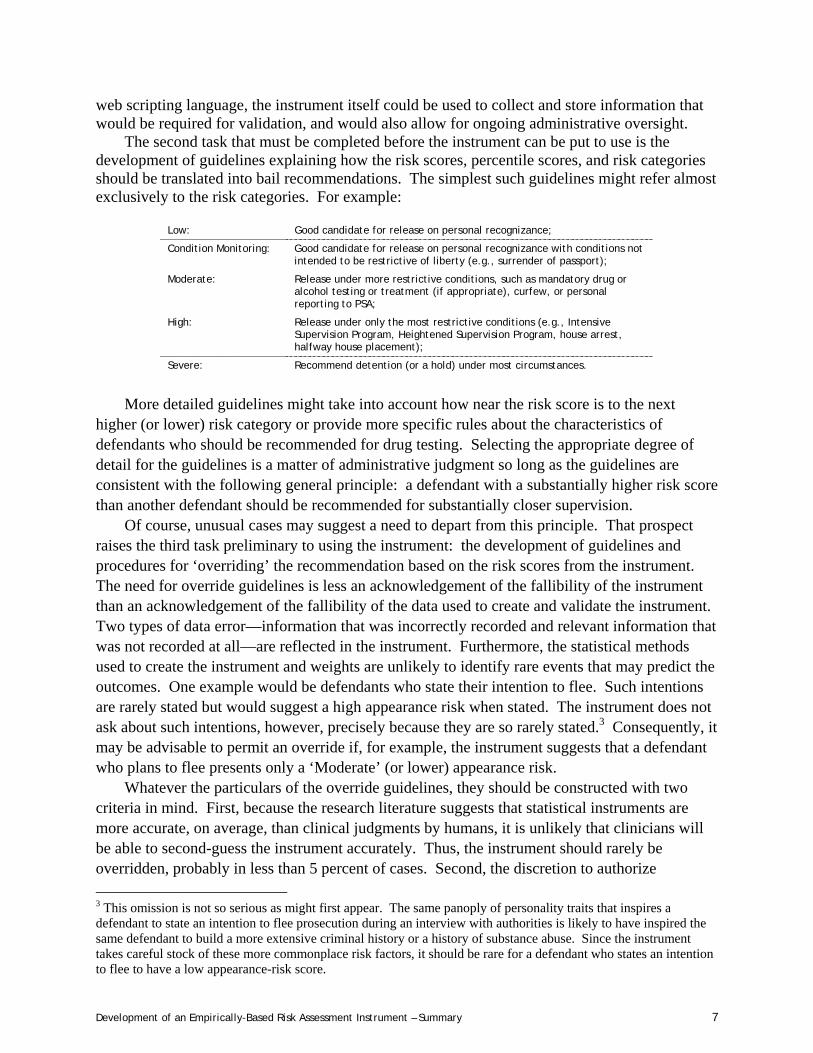
The second task that must be completed before the instrument can be put to use is the development of guidelines explaining how the risk scores, percentile scores, and risk categories should be translated into bail recommendations. The simplest such guidelines might refer almost exclusively to the risk categories. For example:

Low: Good candidate for release on personal recognizance;

Condition Monitoring: Good candidate for release on personal recognizance with conditions not intended to be restrictive of liberty (e.g., surrender of passport);

Moderate: Release under more restrictive conditions, such as mandatory drug or alcohol testing or treatment (if appropriate), curfew, or personal reporting to PSA;

High: Release under only the most restrictive conditions (e.g., Intensive Supervision Program, Heightened Supervision Program, house arrest, halfway house placement);

Severe: Recommend detention (or a hold) under most circumstances.

More detailed guidelines might take into account how near the risk score is to the next

higher (or lower) risk category or provide more specific rules about the characteristics of defendants who should be recommended for drug testing. Selecting the appropriate degree of detail for the guidelines is a matter of administrative judgment so long as the guidelines are consistent with the following general principle: a defendant with a substantially higher risk score than another defendant should be recommended for substantially closer supervision.

Of course, unusual cases may suggest a need to depart from this principle. That prospect raises the third task preliminary to using the instrument: the development of guidelines and procedures for ‘overriding’ the recommendation based on the risk scores from the instrument. The need for override guidelines is less an acknowledgement of the fallibility of the instrument than an acknowledgement of the fallibility of the data used to create and validate the instrument. Two types of data error—information that was incorrectly recorded and relevant information that was not recorded at all—are reflected in the instrument. Furthermore, the statistical methods used to create the instrument and weights are unlikely to identify rare events that may predict the outcomes. One example would be defendants who state their intention to flee. Such intentions are rarely stated but would suggest a high appearance risk when stated. The instrument does not ask about such intentions, however, precisely because they are so rarely stated.3 Consequently, it may be advisable to permit an override if, for example, the instrument suggests that a defendant who plans to flee presents only a ‘Moderate’ (or lower) appearance risk.

Whatever the particulars of the override guidelines, they should be constructed with two criteria in mind. First, because the research literature suggests that statistical instruments are more accurate, on average, than clinical judgments by humans, it is unlikely that clinicians will be able to second-guess the instrument accurately. Thus, the instrument should rarely be overridden, probably in less than 5 percent of cases. Second, the discretion to authorize 3 This omission is not so serious as might first appear. The same panoply of personality traits that inspires a defendant to state an intention to flee prosecution during an interview with authorities is likely to have inspired the same defendant to build a more extensive criminal history or a history of substance abuse. Since the instrument takes careful stock of these more commonplace risk factors, it should be rare for a defendant who states an intention to flee to have a low appearance-risk score.


overrides of the instrument should be vested in as few persons as practicably possible. This is to help ensure that overrides are indeed rare and to provide accountability and uniformity for override decisions.

Ongoing Validation

The validation of a statistical risk-assessment instrument is a continuous process, not a discrete one. Key factors contributing to the performance of such instruments, such as the characteristics of the defendants being screened, the types of information available to screeners, and the quality (i.e., validity) of that information, are continuously changing. The instrument must be updated regularly to keep pace with those changes.

To make the validation of the instrument an ongoing process, it is recommended that PSA collect several pieces of information for each defendant-case screened using the instrument. This information should include: the defendant and case identification numbers, the date of the screening, the responses to each of the items on the instrument, an indicator of whether the assessment of the instrument was overridden, and the reason for any override. Additional information required for an ongoing validation, such as whether the defendant was granted pretrial release and whether the defendant actually had an FTA or arrest while under supervision, may be gleaned from existing PSA data systems (i.e., PRISM, ABADABA).

After collecting these data for a period of 12-18 months after the instrument is put into service, it should be possible for PSA to re-assess the performance of the instrument and re-estimate the weights if its accuracy proves to be substantially less than the estimates from the 1999 study sample suggest. It is also recommended that, as PRISM becomes fully operational, an analysis of the predictive capacity of additional variables also be assessed at the same time that the instrument is validated. This would require additional analyses as well.

Chapter 1. Overview 1

Chapter 1. Overview

PURPOSE OF STUDY

In 2001, the Urban Institute was commissioned by the District of Columbia Pretrial Services Agency (PSA) to develop a risk assessment instrument to assist its diagnosticians in recommending conditions of pretrial release for the thousands of defendants they process each year. This is the final report on the second and final phase of the instrument development. This phase of the research built on the earlier work by extending the period for observing outcomes by 14 months (from nearly two years to three years or longer), expanding the set of predictor items considered for inclusion on the instrument, and searching for combinations of items for inclusion.

The resulting instrument is intended to serve two primary goals. The first goal is to make the development of release recommendations more objective and consistent across defendants. The attainment of this goal should improve the transparency of PSA assessment and recommendation processes to observers both inside and outside the agency. The second goal is to improve the accuracy of decision-making based on risk assessment. Improved accuracy should increase public safety, reduce court costs associated with non-appearance, and reduce the number of low-risk defendants whose liberty is restricted.

The instrument is designed to predict two outcomes, risk of failure-to-appear, or FTA (indicated by issuance of a bench warrant for failure-to-appear), and risk of rearrest (which included either a new arrest record or a citation). Measures that might predict either or both of these two outcomes (i.e., FTA or arrest under supervision) were created from the Automated Bail Agency Data Base (ABADABA) and Drug Testing Management System (DTMS) data. The data included information about the criminal histories, demographics, health, employment, and drug use of all defendants processed by PSA during the study period.

Candidate predictors were constructed from these data. They included items on a list provided by PSA, based on institutional understanding of the characteristics of defendants who fail, and items suggested by UI, based on knowledge of the research literature on the prediction of criminal outcomes. The list was constrained, however, to data in the existing ABADABA and DTMS; some candidate predictors could not be measured with available information. The significant predictors of either outcome (FTA or rearrest) are included in the final instrument.

The assessment instrument was developed using data on a cohort of defendants processed by PSA between January 1, 1999 and June 30, 1999. This time period was selected jointly with PSA because it was: 1) sufficiently recent that changes in the defendant population between 1999 and the present were expected to be of minor importance to the form and function of the instrument, but also 2) sufficiently long ago that nearly all of the defendants would have completed their PSA supervision before the data were provided to UI for analysis.

Chapter 1. Overview 2

The scores on the instrument range from 0 to 100 for each risk outcome. The instrument scoring is designed to assist PSA diagnosticians in prospectively assessing the appearance and safety risk posed by individual defendants. Once a diagnostician has answered all of the questions on the instrument, the instrument weights the answers to compute two risk scores (one each for appearance risk and for safety risk) that range from 0 to 100.1 These scores are then used to classify the level of risk into five categories that could be used when making a release recommendation for court in the bail report. The risk score and risk category could be included in the bail report as well to provide the judge with the benefit of this information.

SUMMARY FINDINGS ON INSTRUMENT


ORGANIZATION OF THE REPORT

In the remaining sections of this report, Chapter 2 presents the research questions and specific methods that were developed to answer them. Chapter 3 and Chapter 4 present, in turn, details on instrument construction and performance. Chapter 5 summarizes the project and provides recommendations for implementation. Full explication of the data processing steps, the variable and file construction, and the findings are contained in the appendices.

1 Although the computation of the risk scores from the answers and weights is purely arithmetic, it is not simple. Even a user who felt competent to perform the computations would shortly find it tedious to perform them with a hand calculator. Ideally, the instrument should be integrated into the management information system used by PSA so that the computer can calculate the scores with little or no input from the user.

Chapter 2. Research Questions and Methods 3

Chapter 2. Research Questions and Methods

RESEARCH QUESTIONS

Three general sets of analytic questions guided the instrument development. Collectively, the responses to these questions provide a thorough examination of the assessment capabilities of the instruments as well as the implications deploying the instruments may have on the number of persons in pretrial detention and the number of persons in resource-intensive supervision programs:

1. What should be included on an empirically-validated risk instrument?

(1.1) What items of information, routinely available to diagnostic Pretrial Services Officers, should be included in an instrument intended to assess prospectively the risk that a defendant will be arrested while under PSA supervision or will FTA while under PSA supervision? How should these items be weighted to assess each outcome? (Chapter 3: Table 3-1 and Ta-ble 3-2)

(1.2) How should the risk scores generated from the instruments be categorized to decide: (a) whether to recommend that a defendant be held or released pending case disposition; and (b) if the defendant is recommended for release, what the level of supervision should be? (Chap-ter 3, Table 3-3)

2. How do the instruments and underlying statistical models perform on the validation sample? (2.1) What is the distribution of risk? Does the proportion of failures increase as the scores in-

crease? (Chapter 4, Figures 4-1 through 4-4)

(2.2) How are the predicted risk scores related to the observed success or failure? (Chapter 4, Figure 4-5 and Figure 4-6)

(2.3) How do the instruments perform at various cut-points? (Chapter 4, Figure 4-7 and Figure 4-8)

(2.4) Under certain decision-rules regarding cut-points (selection rate=base rate), how does the model’s classifications perform? (Appendix D)

(2.5) Does the model distinguish low-risk from high-risk cases? (Chapter 4: Figures 9 and 10)

(2.6) How does the model perform compared to clinical assessments? (Chapter 4, Table 4-1 and Table 4-2)

3. How applicable is the risk instrument to Federal defendants and to those not released (e.g., for use in the initial release decision)?

(3.1) How does the instrument perform when applied to defendants processed in Federal rather than District Court? (Chapter 4, Figures 4-11 and 4-12)

(3.2) How does the instrument perform when applied to detained as opposed to released defen-dants? (Chapter 4, Figures 4-13 and 4-14)


To examine these questions, we selected a sample of cases from the court records of defendants screened by PSA during the first six months of 1999, a time period selected by agreement with PSA to allow a follow up period of 37 to 43 months after a target event that resulted in referral to PSA for screening. The methods used to create variables, select this sample, and construct the instrument are described below.

THE SAMPLE

The unit of analysis for the study was the defendant-case (i.e., each defendant with at least one qualifying case matched with exactly one of their intake-cases). The sample consists of the first eligible criminal case filed against a defendant between January 1, 1999 and June 30, 1999, inclusive. Cases were excluded if they were not prosecuted (over 1,000 cases disposed as ‘no papered’); ended in dismissal or nolle prosequi within 30 days of being opened and before the first scheduled court hearing (41 cases); or were disposed within three days of being opened (541 cases). If a defendant had multiple eligible cases, the first case filed during the study period was selected. If multiple cases were filed on the day of the first eligible case, the case with the most serious charge was selected as the sample case, and the other cases opened the same day were recorded as collateral cases.2 Twenty-one defendants had multiple qualifying cases involving equally serious charges. These 21 defendants had a total of 46 cases opened against them on the date of the first eligible case. One of these cases was selected at random for each of the 21 defendants, and the remaining 25 cases were designated as collateral cases. The final sample thus consisted of 7,574 defendants, each with a single target case selected for the analysis.

The full sample of 7,574 defendant cases was randomly divided into two halves. One half (3,788 cases) was used as a construction sample used to develop the instrument. The other half (3,786 cases) was used as a ‘validation sample,’ to assess the accuracy of the instrument. The method avoids overstating the accuracy of the instrument: When a statistical model is estimated from a data set, the model is tailored to fit the idiosyncrasies of those data. Using the validation sample, with a different set of idiosyncrasies, to assess the accuracy of the instrument will generally yield estimates that more closely reflect how the instrument will perform in practice.

THE DATA

The data used in the study were extracted from PSA data systems during August 2002. The data include an observed follow-up period of 37 to 43 months after the target event date of each defendant. The analysis file includes demographic, employment, health, and criminal history information from the ABADABA relational database management system. Information on drug tests and self-reports of drug use was obtained from the DTMS data system.

Two dependent variables were created from ABADABA data: risk of failure-to-appear as indicated by issuance of a bench warrant for failure-to-appear, and risk of rearrest (for either a 2 The PSA employees who prepared the ABADABA and DTMS data provided UI with the measure of charge seri-ousness that is used in some PSA administrative reports. This seriousness index is not native to ABADABA; it is an adjunct data field.


new arrest or a citation). Both outcomes were limited to events during the study period; neither measure provided any information about the nature (e.g., type of arrest charge) or timing of the FTA or arrest.

More than 100 predictor measures were created for each defendant-case in the sample. These measures spanned several domains including defendant demographics (e.g., age, sex, race, citizenship, and education), personal statistics (e.g., residence in the D.C. metropolitan area, cohabitation with family members, residential tenure), physical and mental health problems, employment status, history of self-reported substance use and drug test results, and a host of criminal history variables. In addition, binary (i.e., ‘yes’ or ‘no’) dummy variables were created to distinguish defendants who were released under PSA supervision from those who were not and to distinguish D.C. defendants from Federal defendants.

Three criteria guided decisions about which measures to create and consider for inclusion on the instrument. The first criterion was to create as many of the measures on the instruments drafted by PSA as possible. UI succeeded in creating all but two of the measures on the draft instruments. UI found that information related to these two omitted measures—any contact with family members or relatives in the past 30 days and any self-reported use of alcohol in the past 30 days—were rarely recorded in PSA database systems.

The second criterion was to thoroughly mine the data for other pieces of information that might predict either FTA or arrest under supervision. One result of this effort was a count of the number of ‘invalid’ drug tests recorded in DTMS for each defendant. An invalid drug test was defined as a test record for which no results were reported because the defendant evaded the test (e.g., by not showing up or by submitting an inadequate or contaminated sample). This count of invalid drug tests proved to be a good predictor of risk of arrest under supervision.

The third criterion was to ensure that the instrument included only items of information that would reasonably be available to PSA at the time of a defendant’s diagnostic interview. In general, this meant that information entered into ABADABA or DTMS more than one day after the date of the defendants’ arrest or citation was ignored. If, for example, new charges were filed against a defendant four days after their 1999 target case, the new charges would not have been included in the count of current charges faced at the time of the diagnostic interview.

A detailed narrative description of the procedures used to create the variables is presented in Appendix B with tables of descriptive statistics for each of the 116 variables in the analysis file.

SAMPLE CHARACTERISTICS

The sample included defendants with different kinds of cases. There were 303 Federal defendants, and 7,271 D.C. defendant cases. The sample also included both defendants who were granted pretrial release (n= 5,708) and those who were not released during the study period (n= 1,866). The characteristics of these sample subgroups is provided in Appendix B, with an analysis of significant differences.

All 7,574 defendants are included in Table B-1; the 303 Federal defendants are included in B-2, and the 7,271 D.C. Superior Court defendant cases in Table B-3. Tables B-4 and B-5


describe, respectively, the 5,708 defendants granted pretrial release and the 1,866 defendants not granted release under PSA supervision.

The differences in subgroups may well affect the extent to which the instrument is appropriate for use with two subgroups of defendants, those facing Federal charges and those not released (who could not be included in the analysis because they had no opportunity for an FTA or arrest on a new charge). The comparison of subgroups in Appendix B shows that the Federal defendants differed from the D.C defendants on a number of variables and, as a result, may have different risks of FTA and rearrest. The Federal defendants were older, better educated, and less likely to be black or unmarried. They were less likely to be U.S. citizens, more likely to be legal aliens, and less likely to be residents of the D.C. metropolitan area. Federal defendants had less extensive criminal histories, and were less likely to have histories of drug use or be interviewed by PSA in lock-up.

Defendants released during the study period also differed from those who were not released on a number of variables. Not surprisingly, those who were not released during the study period were more likely to be male; unmarried; have more extensive criminal histories; greater drug involvement, be interviewed in lock-up; be under PSA supervision at the time the case was filed; and be more likely to have current or pending cases involved charges of escape or Bail Reform Act (BRA) violations. Conversely, women; married defendants; those with less prior criminal and drug involvement; more education; and those who reported living with family, children, or a spouse were more likely to be released.

INSTRUMENT CONSTRUCTION METHODS

Step 1. Refining and Expanding Predictor Measures

Designing a risk-assessment instrument requires identifying a set of measures that jointly predict the outcome of interest. One of the more difficult aspects of this task is identifying measures that are conditionally predictive (e.g., the number of prior arrests may be predictive only among defendants with more than 3 positive drug tests). Failing to identify measures that are conditionally predictive may yield an instrument that is less than optimally accurate. A specialized algorithm, a Chi-squared Automatic Interaction Detector (CHAID), was used to identify predictors defined by combining the values of predictor items.

CHAID systematically splits a set of cases into smaller and smaller groups that are increasingly homogeneous with respect to a specified outcome measure. A set of predictor measures is used to split the cases, and the algorithm uses a statistical test, a chi-squared test, to identify the optimal predictor variable to use for each split. The results of the CHAID algorithm are typically displayed as a classification tree that divides the full sample sequentially into multiple, mutually exclusive groups of the cases. The variable values that define these subgroups were used to define new predictor variables that were added to the data set.


Step 2. Selecting Predictors for the Instrument

Logistic regression was used to select the items for inclusion in the instrument. This procedure has been widely used in the development of similar assessment instruments (see, for example, Gottfredson & Jarjoura, 1996) and is well suited to modeling binary outcomes using a mix of nominal, ordinal, and continuous predictor measures.

Two logistic regression models were estimated for each of the two outcomes on the 2,854 defendants in the construction sample in which pretrial release was granted. The first of these models was a stepwise logistic regression model designed to identify which of the dozens of predictor variables yield the best predictions of the outcome. The stepwise procedure considers all of the available predictor measures, adds to the model the predictor that most improves the ability of the model to reproduce the outcome data (i.e., which defendants succeeded and which failed), considers all of the remaining predictors, adds the best of those to the model, and so on. Stepwise logistic regression models are estimated under the constraint of a criterion specifying how much marginal improvement in the model the addition of another predictor must make before it may be added to the model. The iterative selection of predictors stops when none of the remaining predictors satisfies the criterion. The variables included in the logistic regression are shown in the sample description tables (B-1 to B-5).3 The significant predictors of either of the two outcomes were included in the final instrument.

Step 3. Developing Instrument Scores

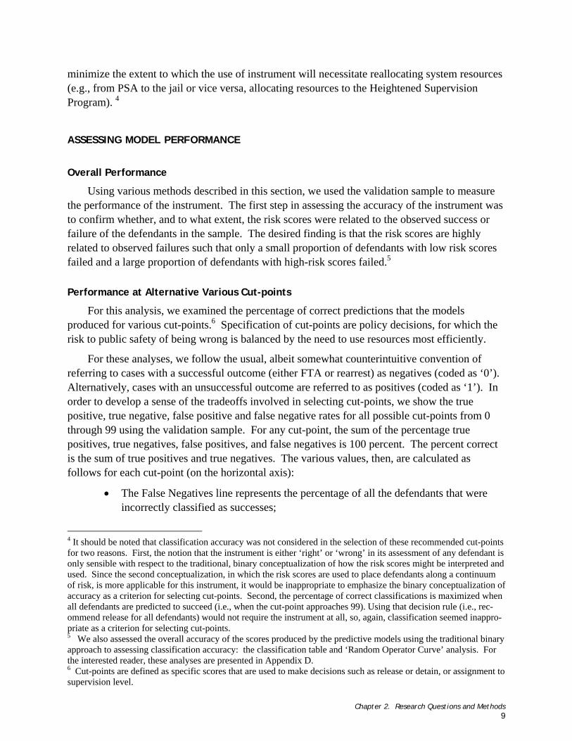
Weights from the logistic regression were used to create a risk score between 0 and 100 for each outcome. The appearance- or safety-risk score, R, was be computed as follows:

( )

( ) 1001 2110

2110

×⎟⎟⎠

⎞⎜⎜⎝

⎛

+= ++++

++++

kk

kk

XBXX

XBXX

eeR βββ

βββ

Κ

Κ

where β0 is the Intercept value, Xk is the numeric answer to the kth question, and βk is the

weight associated with the kth question. Once the formula has been applied to compute an appearance-risk score and a safety-risk score for a defendant, the risk scores should be rounded to the nearest integer.

Step 4. Developing Supervision Level Classification

To divide the risk scores into five risk categories that matched the needs of PSA to use the results for caseload assignment purposes, we used the five supervision levels suggested by PSA as the organizing framework: Low, Condition Monitoring, Moderate, High, or Severe. Two cutpoints (the Condition Monitoring cut-points and the High cut-points) were selected 3 The 28 not included in the logistic regression are marked with an asterisk on the tables. Most excluded variables had missing data for a large number of defendants. Others were created only for descriptive purposes, such as those measuring the number of days between the beginning of pretrial release and the first failure (i.e., an FTA or a new arrest). MALE and BLACK were never intended to be included on the instrument.


arithmetically to match the current distribution of supervision level among defendants under PSA supervision. The Condition Monitoring cut-points were computed as a halving of the odds of failure. The sample base rate for FTA, PA, (among released defendants) was approximately 21.5 percent (Table B-4). The sample base rate for arrest under supervision, PS, was 20.2 percent (Table B-4). The odds of FTA, OA, for a randomly selected defendant in the study sample may be computed as:

A

AA P

PO−

=1

That, expressing 21.5 percent as 0.215, solves to 0.274 to 1 odds. Similarly, the odds of arrest, OS, for a randomly selected defendant in the study sample may be computed as:

S

SS P

PO

−=

1

That solves to 0.253 to 1 odds. To compute a risk score, S, associated with a halving of these odds, the following formula was applied:

100

15.01

15.0

×⎟⎟⎟⎟

⎠

⎞

⎜⎜⎜⎜

⎝

⎛

⎟⎠⎞

⎜⎝⎛

−+

⎟⎠⎞

⎜⎝⎛

−=

PPP

P

S

Where P is either PA or PS (Silver & Chow-Martin 2002). Solving for S using PA yielded 12; solving for S using PS yielded 11. This indicates that defendants with appearance-risk scores under 12 have less than half the odds of having an FTA under supervision as the typical defendant. Safety-risk scores under 11 indicate defendants with less than half the odds of being arrested under supervision. With the Condition Monitoring cut-points for appearance and safety set to 12 and 11, respectively, defendants predicted to have less than half the average risk of failure are placed in the Low risk category.

The recommended High cut-points were identified, in a similarly arithmetic manner, as the risk scores indicating a doubling of the odds of failure. The following formula was used to compute the risk scores, S, associated with a doubling of the odds of failure:

100

121

12

×⎟⎟⎟⎟

⎠

⎞

⎜⎜⎜⎜

⎝

⎛

⎟⎠⎞

⎜⎝⎛

−+

⎟⎠⎞

⎜⎝⎛

−=

PPP

P

S

where P is either PA or PS (Silver & Chow-Martin 2002). Solving for S using PA yielded 35; solving for S using PS yielded 34.

The remaining cut-points, those for the Moderate and Severe risk categories, were selected so as to approximate the distribution of the clinical risk judgments. The proportion of sample defendants placed in each clinical-risk category was used as criterion for selecting cut-points to


minimize the extent to which the use of instrument will necessitate reallocating system resources (e.g., from PSA to the jail or vice versa, allocating resources to the Heightened Supervision Program). 4

ASSESSING MODEL PERFORMANCE

Overall Performance

Using various methods described in this section, we used the validation sample to measure the performance of the instrument. The first step in assessing the accuracy of the instrument was to confirm whether, and to what extent, the risk scores were related to the observed success or failure of the defendants in the sample. The desired finding is that the risk scores are highly related to observed failures such that only a small proportion of defendants with low risk scores failed and a large proportion of defendants with high-risk scores failed.5

Performance at Alternative Various Cut-points

For this analysis, we examined the percentage of correct predictions that the models produced for various cut-points.6 Specification of cut-points are policy decisions, for which the risk to public safety of being wrong is balanced by the need to use resources most efficiently.

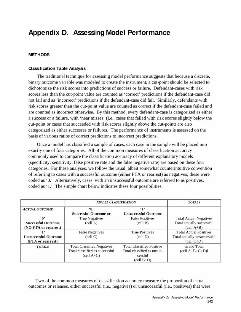
For these analyses, we follow the usual, albeit somewhat counterintuitive convention of referring to cases with a successful outcome (either FTA or rearrest) as negatives (coded as ‘0’). Alternatively, cases with an unsuccessful outcome are referred to as positives (coded as ‘1’). In order to develop a sense of the tradeoffs involved in selecting cut-points, we show the true positive, true negative, false positive and false negative rates for all possible cut-points from 0 through 99 using the validation sample. For any cut-point, the sum of the percentage true positives, true negatives, false positives, and false negatives is 100 percent. The percent correct is the sum of true positives and true negatives. The various values, then, are calculated as follows for each cut-point (on the horizontal axis):

• The False Negatives line represents the percentage of all the defendants that were incorrectly classified as successes;

4 It should be noted that classification accuracy was not considered in the selection of these recommended cut-points for two reasons. First, the notion that the instrument is either ‘right’ or ‘wrong’ in its assessment of any defendant is only sensible with respect to the traditional, binary conceptualization of how the risk scores might be interpreted and used. Since the second conceptualization, in which the risk scores are used to place defendants along a continuum of risk, is more applicable for this instrument, it would be inappropriate to emphasize the binary conceptualization of accuracy as a criterion for selecting cut-points. Second, the percentage of correct classifications is maximized when all defendants are predicted to succeed (i.e., when the cut-point approaches 99). Using that decision rule (i.e., rec-ommend release for all defendants) would not require the instrument at all, so, again, classification seemed inappro-priate as a criterion for selecting cut-points. 5 We also assessed the overall accuracy of the scores produced by the predictive models using the traditional binary approach to assessing classification accuracy: the classification table and ‘Random Operator Curve’ analysis. For the interested reader, these analyses are presented in Appendix D. 6 Cut-points are defined as specific scores that are used to make decisions such as release or detain, or assignment to supervision level.


• The False Positive line represents the percentage of all the defendants that were incorrectly classified as failures;

• The True Positive line represents the percentage of defendants correctly classified as having failed;

• The True Negative line represents the percentage of defendants correctly classified as having succeeded;

• The Percent Correct is the total correct predictions divided by the total validation sample.

A starting point for making a decision regarding how best to characterize risk levels can be developed by examining the graphs (presented in Chapter 4) and noting the cut-points at which the lines intersect.

Base Rate Dispersion Analysis

When examining a distribution of risk scores, the underlying instruments can be evaluated based on how well higher-risk defendants are distinguished from lower-risk defendant cases (Silver & Chow-Martin, 2002). This conceptualization recognizes risk, and responses to risk, as varying along a continuum. Consequently, the appropriate assessment criterion is a measure of base-rate dispersion (Silver & Chow-Martin, 2002).

For any risk score, base-rate dispersion is the percentage of defendants with varying risk scores who actually failed. The base-rate dispersion for a risk score of 0 is, by definition, equal to the base rate in the sample. Since all defendants have risk scores greater than or equal to 0, base-rate dispersion is equal to the percentage of the failures in the sample (i.e., the base rate). The more useful the instrument, under this conceptualization, the higher the base-rate dispersion value climbs as the risk score increases.

ASSESSING EXTERNAL VALIDITY OF THE MODEL RESULTS: COMPARISON OF STATISTICAL AND CLINICAL RISK CLASSIFICATION

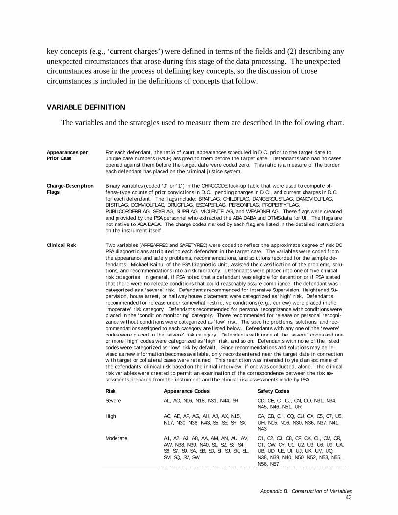
For this analysis we compared the statistical and clinical risk categories in the validation sample. The clinical risk scores were based on the problems, solutions, and recommendations PSA listed for defendants as a basis for the bail recommendation.7 These categories are referred to as assessments of clinical risk because they are based on the judgments of PSA personnel, typically following a personal interview with the defendant. These clinical risk scores were split into the same five categories as were the statistical risk categories, which were derived from the instrument risk scores. These may be referred to as assessments of ‘statistical risk’ because they are computed in formulaic fashion from the answers to the instrument questions. We tested the degree to which there was correspondence between the two sets of scores through a Spearman

7 Several hundred defendants had no problems, solutions, or recommendations recorded for them. Such omissions were interpreted as indicating that the defendant had no discernible problems requiring solutions and that PSA had effectively recommended the defendant for release without supervision.


correlation coefficient.8 If the statistical risk scores created from the instrument were validated, one would expect that defendants placed in higher statistical risk categories also tended to be placed in higher clinical risk categories as well and vice versa.

ASSESSING MODEL APPLICABILITY TO FEDERAL DEFENDANTS AND DETAINEES

In this assessment, we were concerned with understanding the degree to which the model developed on releasees might be able to be used both for cases prosecuted in Federal Court, as well as for the entire set of cases coming before the court prior to the release decision being made (this would, then, include those subsequently detained as well as those released). For these analyses, we applied the statistical models to the validation sample, first examining how the distribution of scores varied for Federal defendants as compared to District Court defendants, and then for detainees as compared to releasees.

8 The Spearman correlation coefficient is an accepted measure of association between two ordinal measures. It ranges from –1 to +1, where –1 indicates a perfect negative association, 0 indicates no association, and +1 indicates a perfect positive association.

Chapter 3. Instrument Construction 12

Chapter 3. Instrument Construction

SELECTION OF PREDICTORS FOR THE INSTRUMENT

The first step was to examine the capacity of combinations of variables to predict the outcomes. CHAID models were estimated using the construction sample to identify subgroups with maximally different average values on the outcome variables (see Appendix C for more detail). The CHAID model of failure-to-appear identified 11 subgroups of defendants that differed significantly on the outcome; the CHAID model of rearrest identified 9 subgroups. Based on these results, 20 new variables, not shown in Tables B-1 through B-5, were created to identify defendants who fit into each of these subgroups. For example, one subgroup was comprised of defendants with no invalid drug tests and no more than two valid drug tests. These variables were then included with the other items in the logistic regression models.

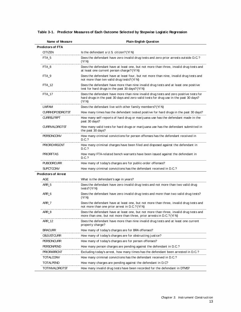
The final instrument consists of 22 items (shown in Table 3-1). The predictors are listed in alphabetical order by the name of the predictor measure. The predictors based on the CHAID results (i.e., those with names ending with an underscore (_) and a numeral) require answers to several questions. On the instrument and Microsoft Excel spreadsheet, the compound questions associated with the CHAID dummy variables in Table 3-1 have been broken out into multiple, simpler questions. This step was taken to make the instrument easier to use.

Nearly all of the predictors are related to drug testing, criminal history, and target arrest charges. However, the items that proved predictive of FTA were different from those that predicted rearrest. Only 3 of the 22 predictors were based on PSA interviews with defendants following arrest (age, citizenship, and whether they share a residence with any members of their family). The remaining 19 items came from items already in ABADABA and DTMS and available as soon as a defendant’s identity has been established. This suggests that the introduction of the instrument may provide an opportunity to either shorten the defendant interviews or re-focus a portion of the interviews on topics that are not routinely addressed (e.g., peer associations, relationship with alleged victim(s), etc.).


Table 3-1. Predictor Measures of Each Outcome Selected by Stepwise Logistic Regression

Name of Measure Plain-English Question

Predictors of FTA

CITIZEN Is the defendant a U.S. citizen? (Y/N)

FTA_5 Does the defendant have zero invalid drug tests and zero prior arrests outside D.C.? (Y/N)

FTA_8 Does the defendant have at least one, but not more than three, invalid drug tests and at least one current person charge? (Y/N)

FTA_9 Does the defendant have at least four, but not more than nine, invalid drug tests and not more than ten valid drug tests? (Y/N)

FTA_12 Does the defendant have more than nine invalid drug tests and at least one positive test for hard drugs in the past 30 days? (Y/N)

FTA_17 Does the defendant have more than nine invalid drug tests and zero positive tests for hard drugs in the past 30 days and zero valid tests for drug use in the past 30 days? (Y/N)

LWFAM Does the defendant live with other family members? (Y/N)

CURRHDPOSDRGTST How many times has the defendant tested positive for hard drugs in the past 30 days?

CURRSLFRPT How many self-reports of hard drug or marijuana use has the defendant made in the past 30 days?

CURRVALDRGTST How many valid tests for hard drugs or marijuana use has the defendant submitted in the past 30 days?

PERSONCONV How many criminal convictions for person offenses has the defendant received in D.C.?

PRIORCHRGCNT How many criminal charges have been filed and disposed against the defendant in D.C.?

PRIORFTAS How many FTA-related bench warrants have been issued against the defendant in D.C.?

PUBODRCURR How many of today's charges are for public-order offenses?

SUPCTCONV How many criminal convictions has the defendant received in D.C.?

Predictors of Arrest

AGE What is the defendant's age in years?

ARR_5 Does the defendant have zero invalid drug tests and not more than two valid drug tests? (Y/N)

ARR_6 Does the defendant have zero invalid drug tests and more than two valid drug tests? (Y/N)

ARR_7 Does the defendant have at least one, but not more than three, invalid drug tests and not more than one prior arrest in D.C.? (Y/N)

ARR_8 Does the defendant have at least one, but not more than three, invalid drug tests and more than one, but not more than three, prior arrests in D.C.? (Y/N)

ARR_12 Does the defendant have more than nine invalid drug tests and at least one current property charge?

BRACURR How many of today's charges are for BRA offenses?

OBJUSTCURR How many of today's charges are for obstructing justice?

PERSONCURR How many of today's charges are for person offenses?

PERSONPEND How many person charges are pending against the defendant in D.C.?

PRIORARRCNT Excluding today's arrest, how many times has the defendant been arrested in D.C.?

TOTALCONV How many criminal convictions has the defendant received in D.C.?

TOTALPEND How many charges are pending against the defendant in D.C?

TOTINVALDRGTST How many invalid drug tests have been recorded for the defendant in DTMS?


INSTRUMENT SCORES

To develop instrument scores from the selected items, it was necessary to recode some variables to eliminate values that could distort the weight assigned to the item. The answers to several of the questions in the initial predictors identified had no theoretical upper limit. For example, Table B-1 shows that about half of the defendants in the study sample had four or more prior arrests in D.C., but at least one defendant had 78 prior arrests. If the question about prior arrests appeared on the instrument without any upper bound, chances are that eventually a defendant with more than 78 prior arrests would be screened. Such a defendant might receive an anomalous risk score because such an unusually large number of arrests was not anticipated when the instrument was developed.

To guard against this eventuality, UI recoded the predictor measures in Table 3-1 that had values in the construction sample greater than 10. Of the predictor measures with values greater than 10, only AGE was excluded from this recoding. The list of recoded measures included: CURRVALDRGTST, PRIORCHRGCNT, PRIORFTAS, SUPCTCONV, PRIORARRCNT, TOTALCONV, TOTALPEND, and TOTINVALDRGTST. Each of these measures was recoded so that defendants with values greater than 10 were assigned a value of 10 instead of their original value. The value 10 was selected as the upper bound for this truncation so that the measures would retain a fairly wide range of variation but the upper bound would still be a reasonably small number.9 One of the questions on the instrument itself, the one regarding total valid drug tests, allows a maximum value of 11, rather than 10, to be recorded. This question appears on the instrument as one of two questions that jointly contribute to the yes-or-no answer to the question associated with one of the CHAID dummies (FTA_9), which asks, in part, whether the defendant has had ten or fewer valid drug tests in the past 30 days. A value of 11 recorded in response to the question about the number of valid drug tests implies a negative response to the question associated with FTA_9.

For the other measures in Table 3-1 with no theoretical upper limit (i.e., CURRHDPOSDRGTST, CURRSLFRPT, PERSONCONV, PUBODRCURR, AGE, BRACURR, OBJUSTCURR, PERSONCURR, and PERSONPEND), UI noted the maximum value of each measure among the defendants in the entire construction sample, including those not granted pretrial release. The phrasing of the question associated with each of these measures was then revised to reflect this maximum value. For example, the question about the number of today’s charges related to person offenses becomes: “How many (up to 8) of today’s charges are for person offenses?” This rephrasing of the questions to note maximum allowable values ensures defendants with unusually high values on any of these measures will not receive anomalous scores and makes the instrument easier to use. All of the questions on the instrument are either yes-or-no questions or require a numeric answer with an explicitly stated maximum allowable value.

9 Trial-and-error testing was conducted to determine whether truncating these variables to numbers larger than 10 would substantially improve the performance of the instrument at some cost in ease of use. No improvement in the performance of the instrument was found when the variables were truncated to higher values.


The truncation and re-estimation has two benefits. First, it precludes defendants with unusually high values from exerting disproportionate influence on the model. Second, it makes the instrument easier to use. The questions corresponding to these variables may now be rephrased to reflect the truncation. For example, the question about prior arrests in D.C. becomes: “Excluding today's arrest, how many (up to 10) times has the defendant been arrested in D.C.?” Now, if a defendant with dozens of arrests is screened, it is unnecessary to count each arrest record to complete the instrument. The screener may simply record that the defendant has ‘10’ prior arrests.

Using the truncated measures, two new logistic regression models were estimated, one FTA model and one arrest model (shown in Appendix C). These two models were estimated only to produce weights for each question that reflect the truncation of the seven measures described above. Table 3-2 lists the predictor measures for each outcome, the questions associated with each rephrased as necessary, and the weights from the second logistic regression models. The weights have been rounded to two decimal places. For each outcome, one additional row, labeled ‘Intercept’, has been added to Table 3-2. The weight corresponding to this row indicates the starting value that each defendant, regardless of their characteristics, begins with when the instrument assesses their risk. To simplify a bit, defendants begin with a risk score proportionate to the Intercept value, and their score increases or decreases from that value depending upon the answers to the questions on the instrument.

Table 3-2. Predictor Measures, Instrument Questions, and Weights for Both Outcomes

Name of Measure Plain-English Question Weight

Predictors of FTA

Intercept Starting Value -0.58

CITIZEN Is the defendant a U.S. citizen? (Y/N) -0.70

FTA_5 Does the defendant have zero invalid drug tests and zero prior arrests outside D.C.? (Y/N)

-1.22

FTA_8 Does the defendant have at least one, but not more than three, invalid drug tests and at least one current person charge? (Y/N)

-0.98

FTA_9 Does the defendant have at least four, but not more than nine, invalid drug tests and not more than ten valid drug tests? (Y/N)

0.80

FTA_12 Does the defendant have more than nine invalid drug tests and at least one positive test for hard drugs in the past 30 days? (Y/N)

0.46

FTA_17 Does the defendant have more than nine invalid drug tests and zero positive tests for hard drugs in the past 30 days and zero valid tests for drug use in the past 30 days? (Y/N)

0.50

LWFAM Does the defendant live with other family members? (Y/N) -0.28

CURRHDPOSDRGTST How many (up to 5) times has the defendant tested positive for hard drugs in the past 30 days?

0.62

CURRSLFRPT How many (up to 4) self-reports of hard drug or marijuana use has the defendant made in the past 30 days?

0.27

CURRVALDRGTST How many (up to 10) valid tests for hard drugs or marijuana use has the defendant submitted in the past 30 days?

-0.15

PERSONCONV How many (up to 6) criminal convictions for person offenses has the defendant received in D.C.?

-0.27

PRIORCHRGCNT How many (up to 10) criminal charges have been filed and dis-posed against the defendant in D.C.?

-0.07


Name of Measure Plain-English Question Weight

PRIORFTAS How many (up to 10) FTA-related bench warrants have been issued against the defendant in D.C.?

0.16

PUBODRCURR How many (up to 3) of today's charges are for public-order of-fenses?

0.46

SUPCTCONV How many (up to 10) criminal convictions has the defendant re-ceived in D.C.?

0.09

Predictors of Arrest

Intercept Starting Value -1.26

AGE What is the defendant's age in years (up to 81)? -0.01

ARR_5 Does the defendant have zero invalid drug tests and not more than two valid drug tests? (Y/N)

-1.71

ARR_6 Does the defendant have zero invalid drug tests and more than two valid drug tests? (Y/N)

-0.53

ARR_7 Does the defendant have at least one, but not more than three, invalid drug tests and not more than one prior arrest in D.C.? (Y/N)

-1.07

ARR_8 Does the defendant have at least one, but not more than three, invalid drug tests and more than one, but not more than three, prior arrests in D.C.? (Y/N)

-0.46

ARR_12 Does the defendant have more than nine invalid drug tests and at least one current property charge?

0.82

BRACURR How many (up to 3) of today's charges are for BRA offenses? -0.56

OBJUSTCURR How many (up to 2) of today's charges are for obstructing justice? 2.48

PERSONCURR How many (up to 8) of today's charges are for person offenses? -0.31

PERSONPEND How many (up to 9) person charges are pending against the defen-dant in D.C.?

-0.26

PRIORARRCNT Excluding today's arrest, how many (up to 10) times has the de-fendant been arrested in D.C.?

0.09

TOTALCONV How many (up to 10) criminal convictions has the defendant re-ceived in D.C.?

-0.04

TOTALPEND How many (up to 10) charges are pending against the defendant in D.C?

0.22

TOTINVALDRGTST How many (up to 10) invalid drug tests have been recorded for the defendant in DTMS?

0.04

For each of the two outcomes, the answer to each question is multiplied by its respective weight, and a formula is used to compute a risk score from the products (shown in Appendix C). The risk scores, for both appearance risk and safety risk, may range in value from 0 to 100 with greater values reflecting greater risk. Questions in Table 3-2 with negative weights reduce the resulting risk score; questions with positive weights increase the risk score. For example, each prior arrest (up to 10) in D.C. (weight=0.09) increases safety risk, but each pending charge for a person offense in D.C. (weight=-0.26) decreases safety risk.

Table 3-3 lists the cut-points selected for both the appearance-risk scores and the safety-risk scores.10 Each cut-point marks the lowest score placed in the associated category, and consequently, the Low cut-points are fixed at zero.

10 These are the same cut-points displayed in the CutPts worksheet of the Microsoft Excel file containing the func-tioning instrument.


Table 3-3. Cut-points To Delimit Risk Scores into Statistical Risk Categories

Type of Risk Risk Category Appearance Safety Low 0 0

Condition Monitoring 12 11

Moderate 14 16

High 35 34

Severe 44 46

THE INSTRUMENT

The Microsoft Excel mock-up of the instrument is designed to be easy to use, even though the logic underlying it is somewhat more complex. The Excel file is comprised of six worksheets—Instrument, Ptiles, CutPts, FTA_Wgts, ARR_Wgts, and Cellcount. The instrument itself is the Instrument worksheet, and it uses information from the other five worksheets to compute the risk scores.

To use the instrument, simply enter numeric responses to each of the 22 questions into the column labeled ‘Responses.’ Microsoft Excel issues a warning if any invalid (i.e., non-numeric) or out-of-range response is entered. Near the top of the instrument is a cell labeled ‘Logical Errors’. To the right of this cell is a cell that checks whether the responses to the questions are logically consistent. For example, the answer to the question about the number of person charges pending against the defendant must not be greater than the answer to the question about the total number of pending charges. A few other logical inconsistencies of this sort are possible. The ‘Logical Errors’ cell checks all of these and displays ‘OK’ if the responses are consistent and ‘ERROR’ otherwise. Risk scores are computed even if a logical error is identified.

To compute the risk scores, the instrument references the weights recorded in the FTA_Wgts and ARR_Wgts worksheets. Changing the weights on those worksheets will change the weights used by the instrument, but making such changes is not recommended.

The computed risk scores are displayed near the top of the instrument. The ‘Raw Risk Score’ is the score computed from the instrument itself. Separate scores are computed for both safety risk and appearance risk. Next to the raw risk scores are the ‘Risk Percentiles’. The percentile scores compare the raw risk scores with the distribution of risk scores in the validation sample. The percentile risk score is proportional to the percentage of defendants in the validation sample with an equal or lesser raw risk score. For example, a raw appearance-risk score of 16 is in the 41st percentile of risk, meaning that 41 percent of the defendants in the validation sample had appearance-risk scores of 16 or less. This implies that 59 percent of cases in the validation sample had appearance-risk scores greater than 16.

Adjacent to the percentile scores are the risk categories. Cut-points are used to place any defendant assessed using the instrument into one of five risk categories based on the computed


raw risk scores. The cut-points, four each for both safety risk and appearance risk, are recorded at the top of the CutPts worksheet. The risk categories range from ‘Low’ to ‘Severe’. For each category there are two cut-points, one each for appearance risk and safety risk. Defendants with raw risk scores greater than or equal to the cut-point value (but less than the cut-point value of the next higher category) are placed in the associated risk category. For example, the appearance and safety cut-points for the ‘Moderate’ risk category are 15 and 16, respectively. The appearance and safety cut-points for the ‘High’ risk category are 35 and 34, respectively. Defendant-cases with appearance-risk scores between 15 and 34 would, therefore, be placed in the ‘Moderate’ category on appearance risk. Defendant-cases with safety-risk scores between 16 and 33 would be placed in the ‘Moderate’ category on safety risk. Since the cut-points define the lower bound of the associated risk category, the cut-points for the ‘Low’ category must be set to 0.

Below the cut-points on the CutPts worksheet are two tables displaying how the cut-points would have categorized the released defendants in the validation sample and the proportion of defendants in each category that succeeded or failed. The values in these tables are responsive to changes in the cut-point values, so this worksheet provides an easy way to estimate the effect any proposed change to the cut-points would have on the performance of the instrument. The tables draw data from the Cellcount worksheet and compute a host of statistics commonly used to assess the accuracy of risk instruments.

Chapter 4. Instrument Performance 19

Chapter 4. Instrument Performance

THE DISTRIBUTION OF RISK

Figures 4-1 and 4-2 show the distri-bution of appearance risk and safety risk, respectively, among defendants (released or not) in the validation sample. The horizontal axis in both figures is the risk score; the vertical axis is the number of defendants. The shaded area, then, indi-cates the number of defendants with each risk score. Although the instrument scores can range from 0 to 100, few de-fendants had appearance risk scores less than 3 or greater than 60; in the valida-tion sample, only 5 percent of defen-dants had appearance- or safety-risk scores greater than 50. The modal ap-pearance-risk scores were 4 and 14. The distribution of safety-risk scores was more distinctly bi-modal, peaking dra-matically at 3, dropping off, and then climbing more slowly to a second peak at 27. As with appearance-risk, safety-risk scores greater than 60 were rare.

Figure 4-1. Distribution of Appearance Risk Predicted from Instrument

0

50

100

150

200

250

300

0 5 10 15 20 25 30 35 40 45 50 55 60 65 70 75 80 85 90 95

Appearance-Risk Score

Num

ber o

f Def

enda

nts

Figure 4-2. Distribution of Safety Risk Predicted from Instrument

0

50

100

150

200

250

300

0 5 10 15 20 25 30 35 40 45 50 55 60 65 70 75 80 85 90 95

Safety-Risk Score

Num

ber o

f Def

enda

nts


A related view of the distribution of risk is the cumulative distribution shown in Figures 4-3 and 4-4. In these figures, the horizontal axis once again indicates the risk score. The vertical axis represents the cumulative percentage of defendants. The height of the line indicates the percentage of defendants with a risk score less than or equal to the value on the horizontal axis. For example, Figure 4-3 indicates that 50 percent of defendants had appearance-risk scores less than or equal to 18; 18 was, therefore, the median appearance-risk score. Approximately 75 percent of de-fendants had appearance-risk scores less than or equal to 30 and 90 percent scored less than 43. Interpreting Figure 4-4 analogously shows that the median safety-risk score was 21, that 75 percent of de-fendants scored less than 29, and that 90 percent of defendants scored below 39.

Figure 4-3. Cumulative Distribution of Appearance Risk Predicted from Instrument

0%

10%

20%

30%

40%

50%

60%

70%

80%

90%

100%

0 5 10 15 20 25 30 35 40 45 50 55 60 65 70 75 80 85 90 95


Cum

ulat

ive

Perc

enta

ge o

f Def

enda

nts

Figure 4-4. Cumulative Distribution of Safety Risk Predicted from Instrument

0%

10%

20%

30%

40%

50%

60%

70%

80%

90%

100%

0 5 10 15 20 25 30 35 40 45 50 55 60 65 70 75 80 85 90 95

Safety-Risk Score

Cum

ulat

ive

Perc

enta

ge o

f Def

enda

nts


ASSESSING MODEL PERFORMANCE

Overall Performance

The first step we took to assess the accuracy of the instrument was to confirm whether, and to what extent, the risk scores are related to the observed success or failure of the defendants in the sample. The desired finding is that the risk scores are strongly related with observed failures such that only a small proportion of defen-dants with low risk scores failed and a large proportion of defendants with high risk scores failed. Figures 4-5 and 4-6 display the results of this comparison for the appearance-risk scores and the safety-risk scores, respectively. Again, for both figures, the horizontal axis displays each specific risk score while the vertical axis displays the percent of defendants with a given score who either failed to appear (Figure 4-5) or were rearrested (Figure 4-6). Both figures reflect the risk scores only of those defendants in the validation sample granted pretrial release.

Figure 4-5 shows that for each 1-point increase in the risk scores, there is an ap-proximately 1-percentage-point increase in the proportion of defendants who failed. Defendant-cases with appearance-risk scores of 4 or 5 failed approximately 10 percent of the time. Defendant-cases with appearance-risk scores of 20 or 21 failed approximately 25 percent of the time, and so on. As the appearance-risk score in-creases toward 50 so too does the percentage of defendants who failed. Since few sample defen-dants received scores as high as 50, the line on the figure becomes increasingly jagged as the risk scores increase. Figure 4-6 shows that a similar relationship exists between the safety-risk scores and the proportion of defendants who failed.

Figure 4-5. Distribution of Appearance Risk by Observed Outcome (among Released Defendants in the Validation Sample)

0%

10%

20%

30%

40%

50%

60%

70%

80%

90%

100%

0 5 10 15 20 25 30 35 40 45 50 55 60 65 70 75 80 85 90 95


Perc

enta

ge o

f Def

enda

nts

Who

Fai

led

To

App

ear

Figure 4-6. Distribution of Safety Risk by Observed Outcome (among Released Defendants in the Validation Sample)

0%

10%

20%

30%

40%

50%

60%

70%

80%

90%

100%

0 5 10 15 20 25 30 35 40 45 50 55 60 65 70 75 80 85 90 95

Safety-Risk Score

Perc

enta

ge o

f Def

enda

nts

Arr

este

d


Performance at Alternative Cut-points

Figures 4-7 and 4-8 present the changes in predictive accuracy that occur as the predicted score changes. The hori-zontal axis shows the percentage of defen-dants, for each score or cut-point, that are correctly predicted (true negatives – those who successfully completed supervision, and true positives – those who unsuccess-fully completed) and those who are incor-rectly predicted (false negatives – those incorrectly predicted to succeed on super-vision, and false positives – those incor-rectly predicted to fail on supervision).11

This information may be reviewed to help decide on a score that might be used to either make the detention decision (e.g., a recommendation to release would never be made for those with scores above, say, 52) or to determine supervision level (e.g., a recommendation for ‘low’ supervision would be made for those who scored 11 or less). Selecting a particular mix of true positives and false negatives is largely a matter of balancing the competing de-mands of public safety versus civil liberty, as well as a decision that will necessarily be informed by limits on the available re-sources.

For both the appearance-risk scores (Figure 4-7) and the safety-risk scores (Figure 4-8), the range of cut-points that optimizes the balance between correct and incorrect predictions is approximately between 25 and 35. The optimal cut-point will lie some-where to the right (on the horizontal axis of the figure) of the rapid decline in false positives and the similarly rapid increase in true negatives. Tables E-1 and E-2, which display the same in-formation in tabular form, are presented in Appendix E.

11 Readers should be reminded that for these analyses, we follow the usual, albeit somewhat counterintuitive con-vention of referring to cases with a successful outcome (either FTA or rearrest) as negatives; these were coded as ‘0.’ Alternatively, cases with an unsuccessful outcome are referred to as positives, coded as ‘1.’

Figure 4-7. Percentage of Correct and Incorrect Appearance Predictions across All Possible Cut Points (among Released Defendants in the Validation Sample)

0%

10%

20%

30%

40%

50%

60%

70%

80%

90%

100%

0 5 10 15 20 25 30 35 40 45 50 55 60 65 70 75 80 85 90 95

Cut PointPe

rcen

tage

of D

efen

dant

-Cas

es False Positives Percent Correct

True Negatives

False Negatives

True

Figure 4-8. Percentage of Correct and Incorrect Safety Predictions across All Possible Cut Points (among Released Defendants in the Validation Sample)

0%

10%

20%

30%

40%

50%

60%

70%

80%

90%

100%

0 5 10 15 20 25 30 35 40 45 50 55 60 65 70 75 80 85 90 95

Cut Point

Perc

enta

ge o

f Def

enda

nt-C

ases False Positives Percent Correct

True Negatives

False Negatives

True Positives


Base Rate Dispersion Results

Figures 4-9 and 4-10 plot the base-rate dispersion value for appearance-risk scores from 0 through 61. The horizontal axis here displays the predicted score, while the vertical axis displays the percent of defendants with equal or greater scores that actually failed. If the score was cor-rectly distinguishing successes from fail-ures, then we would expect to see this per-cent increase as the scores increased. Fewer than 50 defendants had risk scores greater than 61, so the base-rate dispersion value became unstable at higher risk scores.

When looking at Figure 4-9, the plot shows that the base-rate dispersion values climb steadily as the risk score increases, approaching, but not reaching, the 50 per-cent mark. Figure 4-10 plots the base-rate dispersion of the safety-risk scores over the same range and reveals a similar pat-tern. There are no generally accepted rules for assessing whether a given degree of base-rate dispersion is satisfactory.

Figure 4-9. Base Rate Dispersion of Appearance Risk (among Released Defendants in the Validation Sample)

0%

10%

20%

30%

40%

50%

60%

70%

80%

90%

100%

0 5 10 15 20 25 30 35 40 45 50 55 60


Pct o

f Def

enda

nts

with

Equ

al/G

reat

er R

isk

Who

Fai

led

Figure 4-10. Base Rate Dispersion of Safety Risk (among Released Defendants in the Validation Sample)

0%

10%

20%

30%

40%

50%

60%

70%

80%

90%

100%

0 5 10 15 20 25 30 35 40 45 50 55 60

Safety-Risk Score

Pct o

f Def

enda

nts

with

Equ

al/G

reat

er

Ris

k W

ho F

aile

d


ASSESSING EXTERNAL VALIDITY OF THE MODEL RESULTS: COMPARISON OF STATISTICAL AND CLINICAL RISK CLASSIFICATION

Crosstabulating the statistical and clinical risk categories risk categories for appearance risk among all defendants in the validation sample is presented in Table 4-1.12 As expected, the statistical and clinical assessments are associated in a positive direction as indicated by the Spearman correlation coefficient.13 That is, defendants placed in higher statistical risk categories also tended to be place in higher clinical risk categories as well and vice versa.

Table 4-1. Appearance Risk: A Comparison of Statistical and Clinical Risk Categories

Clinical Risk Count Percentage

Low Cond. Mon. Moderate High Severe Total

322 93 473 47 48 993 Low

27%

43 6 98 16 16 179 Cond. Mon.

5%

409 52 994 192 133 1,780 Moderate

49%

67 2 177 45 44 335 High

9%

74 0 135 77 64 350

Statistical Risk

Severe 10%

915 153 1,887 377 305 3,637

Total

25% 4% 52% 10% 8% 100%

Spearman Correlation:

-All Validation Sample Defendant-Cases .21

-Released Validation Sample Defendant-Cases .18

-Non-Released Validation Sample Defendant-Cases .28

Computing the Spearman correlation separately for the released and non-released defendants in the validation sample showed that the clinical and statistical assessment were somewhat more congruent among non-released defendants. This finding suggests that using an instrument that was developed on released cases did not reduce the validity of the instrument’s assessment of detainees. Analogous procedures using the clinical and statistical assessments of safety risk yielded similar findings (see Table 4-2).

12 The statistical risk categories were computed using the cut-points where the selection ratio equals the base rate (presented in Appendix D); changing the cut-points would, of course, change the crosstabulation. 13 The Spearman correlation coefficient is an accepted measure of association between two ordinal measures. It ranges from –1 to +1, where –1 indicates a perfect negative association, 0 indicates no association, and +1 indicates a perfect positive association.


Table 4-2. Safety Risk: A Comparison of Statistical and Clinical Risk Categories

Clinical Risk Count Percentage

Low Cond. Mon. Moderate High Severe Total

544 0 499 10 28 1,081 Low

29%

152 0 199 7 14 372 Cond. Mon.

10%

589 0 1,029 20 92 1,730 Moderate

46%

112 0 209 6 33 360 High

10%

75 0 133 5 28 241

Statistical Risk

Severe 6%

1,472 0 2,069 48 195 3,784

Total

39% 0% 55% 1% 5% 100%

Spearman Correlation:

-All Validation Sample Defendant-Cases .16

-Released Validation Sample Defendant-Cases .09

-Non-Released Validation Sample Defendant-Cases .28

Nonetheless, in spite of the positive correlation found between the statistical and clinical assessments, it must be said that the overall correlation is not as high as would be desirable. Typically, ‘strong’ relationships are those that approach .33 or higher; these relationships are not as strong. However, the locus of the discrepancy between the statistical and the clinical score is not known at the present time; we do know that the algorithm developed to calculate the clinical risk scores produces values which classify approximately half the sample as moderate risk (rather than any of the other four categories). This over-representation of a single clinical risk score will, by necessity, decrease the correlation between the two scores. Because our computer calculations were made in the abstract retrospectively, perhaps the best recommendation would be that PSA should calculate both sets prospectively (statistical and clinical) and compare over time.

ASSESSING MODEL APPLICABILITY FOR FEDERAL DEFENDANTS AND DETAINEES

The evidence in Chapter 2 pointed to some noteworthy differences between the small number of Federal Court defendants processed by PSA and the larger number of D.C. court defendants processed by PSA. Differences were also found between defendants in which pretrial release was granted and those in which it was not granted. As a consequence of these differences, it is important to assess the degree to which instrument could be used for these different groups (Federal Court cases, and detainees). The concern was that the instrument might not accurately assess Federal defendants because there were so few of them among the released defendants in the construction sample. Similarly, only those in the construction sample who


were released contributed to the development of the instrument itself. This exclusion was necessary because it could not be determined whether the non-released defendants would have succeeded or failed if they had been released. With the instrument created and cut-points selected, it was possible to examine more directly whether those concerns were warranted.

Performance for Federal Court Cases

Figure 4-11 shows the distribution of appearance-risk scores for Federal and D.C. defen-dants. Since the vertical axis represents the percentage of defendants in each court that received a specific predicted score, the two distributions may be easily compared. The figure shows that, on average, Federal Court defendants received substantially lower appearance-risk scores than D.C.-court defendants. This observation is consistent with expectations. Few of the measures that best distinguished Federal and D.C. defendants in Table B-6 were selected onto the appear-ance-risk instrument. When examining those measures significantly related to court that were selected for the appearance-risk instrument, most suggest that Federal defendants were lower risks than D.C. defendants. For example, several of the drug-related measures were predictive of court and included as predictors of appearance risk; those cases with higher values were more likely to be DC cases rather than Federal cases.

Figure 4-11. Distribution of Appearance Risk by Court

0%2%4%6%8%

10%12%14%

0 5 10 15 20 25 30 35 40 45 50 55 60 65 70 75 80 85 90


Pct o

f U.S

. Def

enda

nts

0%2%4%6%8%

10%12%14%

0 5 10 15 20 25 30 35 40 45 50 55 60 65 70 75 80 85 90


Pct o

f D.C

. Def

enda

nts

The distribution of safety-risk scores, by court, is shown in Figure 4-12. Nearly half (44 percent) of Federal defendants, as compared to only 16 percent of D.C. defendants, received a safety-risk score of 4 or less. Among the Federal defendants, the distribution of safety risk is


distinctly bi-modal: There is a low-risk group of Federal defendants with little or no criminal history or drug history, and a slightly larger group of higher-risk Federal defendants. By contrast, the instrument suggests that safety risk is more uniformly distributed among D.C. defendants. This suggests that there may be distinct risk groups among Federal defendants. Unfortunately, there are too few Federal defendants in the sample to explore this suggestion in detail. Nevertheless, these risk distributions provide no reason to suspect that the instrument will assess Federal defendants less accurately than D.C. defendants.

Figure 4-12. Distribution of Safety Risk by Court

0%

5%

10%

15%

20%

25%

0 5 10 15 20 25 30 35 40 45 50 55 60 65 70 75 80 85 90

Safety-Risk Score

Perc

enta

ge o

f U.S

. Def

enda

nts

0%

5%

10%

15%

20%

25%

0 5 10 15 20 25 30 35 40 45 50 55 60 65 70 75 80 85 90

Safety-Risk Score

Perc

enta

ge o

f D.C

. Def

enda

nts

Performance for Detained Cases

A similar analysis of Figures 4-13 and 4-14, which depict the distribution of appearance and safety risk by release status leads to more questions than answers. The distribution of appearance- and safety-risk scores among non-released defendants is nearly identical to the distribution among released defendants. One would expect that if defendants are detained because they are seen as higher risk, then the risk scores would be higher. However, this is not the case.


Figure 4-13. Distribution of Appearance Risk by Release Status

0%

2%

4%

6%

8%

0 5 10 15 20 25 30 35 40 45 50 55 60 65 70 75 80 85 90


Pct o

f Rel

ease

d D

efen

dant

s

0%

2%

4%

6%

8%

0 5 10 15 20 25 30 35 40 45 50 55 60 65 70 75 80 85 90


Pct o

f Non

-Rel

ease

d D

efen

dant

s

Figure 4-14. Distribution of Safety Risk by Release Status

0%

2%

4%

6%

8%

0 5 10 15 20 25 30 35 40 45 50 55 60 65 70 75 80 85 90

Safety-Risk Score

Pct o

f Rel

ease

d D

efen

dant

s

0%

2%

4%

6%

8%

0 5 10 15 20 25 30 35 40 45 50 55 60 65 70 75 80 85 90

Safety-Risk Score

Pct o

f Non

-Rel

ease

d D

efen

dant

s


It could be possible that defendants denied pretrial release are no more likely to fail than defendants who are granted pretrial release, and that the instrument may have assessed the non-released defendants accurately. Suggestively, many of the variables most strongly related to detention (see Table B-7) were also selected for the risk-assessment instruments; that is, those variables that determined whether or not a defendant was detained were also important in determining failure to appear or rearrest. However, some of those measures (e.g., BRACURR and PRIORCHRGCNT) have negative weights on the instrument; this means that those defendants with more Bail Reform Act charges (measured by BRACURR) were less likely to fail on pretrial release. This is counterintuitive; common sense suggests that the greater the number of Bail Reform Act (BRA) charges a defendant is facing, the greater the appearance risk.

However, in this instance common sense may be in error. First, BRACURR was not included on the appearance-risk instrument, suggesting that the number of BRA charges a defendant faces is not substantially related to appearance risk at all. Second, BRACURR does appear on the safety-risk instrument but the associated weight is negative. According to the instrument, defendants facing BRA charges are, on average, less likely to be arrested on pretrial release than defendants who are not facing BRA charges. This leaves a choice between accepting that common sense may be in error on this point and that, consistent with the differences in the groups described in Chapter 2, the instrument may be inappropriate for assessing detained defendants. Further, there could also be information not available to this research that is considered by decision makers that is not reflected and could alter the importance of the variables selected. Unfortunately, without additional data about how the instrument performs in practice, it is not possible to revise the instrument appropriately if it were judged suspect. Again, UI suggests that DC Pretrial implement the instrument and conduct a prospective validation study. In this study, not only should the current set of variables be validated, but additional possible predictive information should also be included. This would both expand the set of predictors and adjust the weights of variables identified.

Chapter 5. Summary and Recommendations 30

Chapter 5. Summary and Recommendations

THE INSTRUMENT

The Risk Prediction Instrument is comprised of 22 items, making up two subscales: the Safety Risk Scale and the Appearance Risk Scale. The instrument is designed to predict two outcomes, risk of failure-to-appear, or FTA (indicated by issuance of a bench warrant for failure-to-appear), and risk of rearrest (which included either a new arrest record or a citation). Measures that might predict either or both of these two outcomes (i.e., FTA or arrest under supervision) were created from the ABADABA and DTMS data. The data included information about the criminal histories, demographics, health, employment, and drug use of defendants processed by PSA.

Items were selected for inclusion if they were significantly related to subsequent arrest or failure to appear at court hearings, based on analysis of a sample of defendants from the first half of 1999. Nearly all selected items relate to drug testing, criminal history, and current charges. However, the items that proved predictive of FTA were different from those that predicted rearrest. Most of the items (19 of 22) were based on data routinely stored ABADABA and DTMS and available as soon as a defendant’s identity has been established. The remaining three items were based on PSA interviews with defendants following arrest (age, citizenship, and whether they share a residence with any members of their family).

Scores on the two subscales are based on weights developed to maximize the correct prediction of risk. To make decisions based on the scores, we have provided cut-points that divide defendants into five groups, based on the supervision categories in use at PSA. We also provide figures and associated tables (Appendix E) that describes subscale performance at every possible cut point from 0 to 100 to allow PSA to assess the results of shifting the cut points.


Our analysis of instrument performance found that overall accuracy of predicting a failure reached a maximum of approximately 80 percent on both the Appearance and Safety Risk Scales. The correlation (Spearman R) of the Scale categories developed to match PSA


supervision categories was .21 for Appearance Risk and .16 for Safety Risk. These are modest correlations and suggest that much variance in risk is not explained. Typically, ‘strong’ relationships reach .33 or higher. In part this may result from classifying nearly half the sample in one category (moderate risk).

When applying the instrument to Federal defendants, we found that on average, the Federal Court defendants received lower appearance- and safety-risks scores than D.C. court defendants. This appears to be primarily due to differences between the two groups on the drug-related variables, with the Federal defendants having less severe outcomes than those being handled in the DC Court. We also found little difference in the Appearance and Safety Risk between detained defendants and those released to pretrial supervision, despite our expectation that detainees would have higher risk scores.

The results indicate that the instrument can be used to assist decision-making through standardization; however, because it could only use extant information it only does a fair job of prediction. We strongly suggest that there be prospective validation that would be done through implementing the instrument on a trial basis and re-analyzing the validity of the current set of predictors as well as any additional predictors being collected by the new computer system, Pretrial Real-time Information System Manager (PRISM).

USING THE SPREADSHEET

We have created a Microsoft Excel spreadsheet that can be used to score cases coming into the DC PSA Diagnostic Unit. To use the instrument, simply enter numeric responses to each of the 22 questions into the column labeled ‘Responses.’ To compute the risk scores, the instrument references the weights recorded in the FTA_Wgts and ARR_Wgts worksheets. Changing the weights on those worksheets will change the weights used by the instrument, but making such changes is not recommended.

The computed risk scores are displayed near the top of the instrument. The ‘Raw Risk Score’ is the score computed from the instrument itself. Separate scores are computed for both safety risk and appearance risk. Next to the raw risk scores are the ‘Risk Percentiles’. The percentile scores compare the raw risk scores with the distribution of risk scores in the validation sample, with the percentile risk score proportional to the percentage of defendants in the validation sample with an equal or lesser raw risk score.

Adjacent to the percentile scores are the risk categories. Cut-points are used to place any defendant assessed using the instrument into one of five risk categories based on the computed raw risk scores. The risk categories range from ‘Low’ to ‘Severe’. For each category there are two cut-points, one each for appearance risk and safety risk. Defendants with raw risk scores greater than or equal to the cut-point value (but less than the cut-point value of the next higher category) are placed in the associated risk category.


SPECIAL CONSIDERATIONS AND LIMITATIONS

The development of the instrument was complicated by two factors, both of which were anticipated from the beginning of the project. First, approximately one-fourth of the defendants included in the study were not released under PSA supervision in connection with the 1999 cases we examined. This group included a mixture of defendants who were held in detention pending case disposition as well as a number of defendants whose cases were disposed before they could be placed under PSA supervision. Consequently, no data were available about whether these defendants failed (i.e., had an FTA or arrest) under supervision. As a result, decisions about which questions should appear on the instrument and how the answer to each should be weighted to compute the assessment scores were based exclusively on an examination of the characteristics of those defendants who were released under PSA supervision during the study period. The accuracy of the instrument in assessing the risks posed by defendants like those who were not released cannot be directly examined.

The second complication is that, unlike most pretrial services agencies, PSA processes and supervises defendants for two courts: (1) the D.C. Superior Court and (2) the U.S. District Court for D.C. Only about one in twenty-five defendants processed by PSA are Federal Court defendants, but the Federal defendants differ from the D.C. defendants in many respects. The Federal defendants were less likely to be facing charges related to person offenses and more likely to be married, for example. Released and supervised Federal defendants were included in the analytic sample; nonetheless, because the Federal defendants comprised such a small proportion (about 3 percent) of the sample of defendants that there is some cause for concern that the instrument may not assess Federal defendants as accurately as D.C. defendants. That concern notwithstanding, the instrument assessed the Federal defendants in the study sample as accurately as it assessed the D.C. defendants.

Although this instrument has not been validated on detainees, and was validated using only a small number of Federal defendants, we suspect that neither of these limitations is especially serious. For a variety of reasons, defendants where pretrial release is not granted probably have widely varying degrees of appearance risk and safety risk. Some defendants are not granted pretrial release for reasons largely unrelated to the risks they pose, as, for example, when another jurisdiction requests that they be held and extradited. Federal defendants are also similarly heterogeneous with respect to the risks posed. It is likely that the form of the instrument would be little different if it had been validated on a larger sample of Federal defendants. It is UI’s recommendation that the instrument may be used to assess Federal defendants, but that the application of the instrument to Federal defendants should be undertaken with an extra degree of circumspection. The instrument appears to be suitable for assessing defendants prior to the release decision being made and for defendants being processed in Federal Court so long as a systematic effort at ongoing validation is put into place (see discussion in the next section).


RECOMMENDATIONS FOR USE AND FUTURE DEVELOPMENT

This section chapter offers some guidance about how to use the instrument, discusses the limitations of the instrument, and recommends how the process of validating the instrument should be continued.

Using The Instrument

To begin using the instrument to assess defendants prospectively, three additional tasks must be completed. First, the instrument itself must be implemented in a web scripting language (e.g., ASP, ColdFusion, or PHP) and made available (e.g., on an intranet) to those PSA employees who interview defendants and make bail recommendations. The arithmetic required to compute the risk scores is too complex for human operators to perform efficiently by hand. Using computers would improve the speed and accuracy of the calculations. Implementing the instrument as a dynamic web script will also allow centralized administrative control over the cut-points (and the weights).14 Such a web script could be written to record key pieces of information (e.g., defendant identification number, case identification number, responses to each instrument question, and the risk scores) for each defendant screened in a database. Such a database would permit continuous administrative oversight of the manner in which the instrument was being used and would provide information necessary for the sort of ongoing validation process recommended later in this chapter. Finally, the web script could eventually be integrated into the primary databases used by PSA staff (e.g., PRISM and DTMS), so the correct responses to the questions could be automatically retrieved from those databases without any additional keystrokes from human operators. If the instrument is implemented using a dynamic web scripting language, the instrument itself could be used to collect and store information that would be required for validation, and would also allow for ongoing administrative oversight.

The second task that must be completed before the instrument can be put to use is the development of guidelines explaining how the risk scores, percentile scores, and risk categories should be translated into bail recommendations. The simplest such guidelines might refer almost exclusively to the risk categories. For example:

Low: Good candidate for release on personal recognizance;

Condition Monitoring: Good candidate for release on personal recognizance with conditions not intended to be restrictive of liberty (e.g., surrender of passport);

Moderate: Release under more restrictive conditions, such as mandatory drug or alcohol testing or treatment (if appropriate), curfew, or personal report-ing to PSA;

High: Release under only the most restrictive conditions (e.g., Intensive Super-vision Program, Heightened Supervision Program, house arrest, halfway house placement);

Severe: Recommend detention (or a hold) under most circumstances.

14 It may be appropriate for PSA administrators to make adjustments to the cut-points recommended in Chapter 4, and the Microsoft Excel file should assist efforts to examine what effect any change of the cut-points would have on the distribution of defendants across the five risk categories before the change is implemented. Nonetheless, the weights should only be changed after a comprehensive empirical examination of the instrument’s performance, and a consideration of the impact that changes might have on all of the weights, not just a few. Because computing the risk scores involves a non-linear (i.e., logarithmic) transformation of the products of the question responses and weights, revising the weights without the benefit of a comprehensive, empirical study is likely to have unexpected effects on the distribution of risk scores.


More detailed guidelines might take into account how near the risk score is to the next higher (or lower) risk category or provide more specific rules about the characteristics of defendants who should be recommended for drug testing. Selecting the appropriate degree of detail for the guidelines is a matter of administrative judgment so long as the guidelines are consistent with the following general principle: A defendant with a substantially higher risk score than another defendant should be recommended for substantially closer supervision.

Of course, unusual cases may suggest a need to depart from this principle. That prospect raises the third task preliminary to using the instrument: The development of guidelines and procedures for ‘overriding’ the recommendation based on the risk scores from the instrument. The need for override guidelines is less an acknowledgement of the fallibility of the instrument than an acknowledgement of the fallibility of the data used to create and validate the instrument. Two types of data error—information that was incorrectly recorded and relevant information that was not recorded at all—are reflected in the instrument. Furthermore, the statistical methods used to create the instrument and weights are unlikely to identify rare events that may predict the outcomes. One example would be defendants who state their intention to flee. Such intentions are rarely stated, but when they are they plainly suggest a high appearance risk. The instrument does not ask about such intentions, however, precisely because they are so rarely stated.15 Consequently, it may be advisable to permit an override if, for example, the instrument suggests that a defendant who plans to flee presents only a ‘Moderate’ (or lower) appearance risk.

Whatever the particulars of the override guidelines, they should be constructed with two criteria in mind. First, because the research literature suggests that statistical instruments are more accurate, on average, than clinical judgments by humans, it is unlikely that clinicians will be able to second-guess the instrument accurately. Thus, the instrument should rarely be overridden, probably in less than 5 percent of cases. Second, the discretion to authorize overrides of the instrument should be vested in as few persons as practicably possible. This is to help ensure that overrides are indeed rare and to provide accountability and uniformity for override decisions.

Ongoing Validation

The validation of a statistical risk-assessment instrument is a continuous process, not a discrete one. Key factors contributing to the performance of such instruments, such as the characteristics of the defendants being screened, the types of information available to screeners, and the quality (i.e., validity) of that information, are continuously changing. The instrument must be updated regularly to keep pace with those changes.

To make the validation of the instrument an ongoing process, it is recommended that PSA collect several pieces of information for each defendant-case screened using the instrument. This information should include: the defendant and case identification numbers, the date of the

15 This omission is not so serious as might first appear. The same panoply of personality traits that inspires a defen-dant to state an intention to flee prosecution during an interview with authorities is likely to have inspired the same defendant to build a more extensive criminal history or a history of substance abuse. Since the instrument takes careful stock of these more commonplace risk factors, it should be rare for a defendant who states an intention to flee to have a low appearance-risk score.


screening, the responses to each of the items on the instrument, an indicator of whether the assessment of the instrument was overridden, and the reason for any override. Additional information required for an ongoing validation, such as whether the defendant was granted pretrial release and whether the defendant actually had an FTA or arrest while under supervision, may be gleaned from existing PSA data systems (i.e., PRISM, ABADABA).

After collecting these data for a period of 12-18 months after the instrument is put into service, it should be possible for PSA to re-assess the performance of the instrument and re-estimate the weights if its accuracy proves to be substantially less than the estimates from the 1999 study sample suggest. It is also recommended that, as PRISM becomes fully operational, an analysis of the predictive capacity of additional variables also be assessed at the same time that the instrument is validated. This would require additional analyses as well.

Appendix A. Data Processing 36

Appendix A. Data Processing

This appendix includes a detailed discussion of the procedures UI used to complete the initial processing of the study data. It will be of interest to persons who are acquainted with the Automated Bail Agency Data Base (ABADABA), and those who are attempting to replicate the study in whole or in part (e.g., those persons tasked with integrating the instrument into the new Pretrial Real-time Information System Manager [PRISM] database PSA has begun to use).

INITIAL DATA PROCESSING

After identifying the relational structure of the ABADABA database, UI processed each data table. Only variables (or ‘fields’) for which a later use was anticipated were retained. Tables related to look-up tables were joined with their look-up tables, and useful fields from the look-up tables were also retained.

The ABADABA database includes tables at several levels of aggregation, including the Bail Agency ID (BAID) or defendant level, the BACE or case level, and the charge-level. During the initial cleaning and recoding phase, no data tables were collapsed to a higher level of aggregation.

Where it was determined that text fields contained potentially valuable information, these were recoded into numeric variables suitable for analysis. Since much of the information recorded in such text fields is inherently imprecise, recoding these text fields required us to make thousands of interpretive judgments. In the interest of efficiency, a single member of our team (Mark Coggeshall) made all of these judgments, and the judgments were coded so as to permit the individual review and revision of each. The following notes provide an overview of the more important of these judgments:

In the NAMEDETAIL table, an undocumented RACE code (‘N’) was recoded to missing, and an undocumented SEX code (‘U’) was recoded to missing. The variable measuring years of educational attainment (YEARSEDUCATION) ranged from 0 to 914; values greater than 20 were recoded to 20. The variable LIVESWITHSPOUSE was recoded to 0 (indicating that the defendant does not live with a spouse) in all cases where marital status was coded as single, divorced, or widowed. The RACE variable included distinct codes for ‘Caucasian’ and ‘White’, but these were collapsed into a single code on the assumption that there is no relevant difference between these designations.

Since date of birth (from which age is computed), sex, and race are such important meas-ures in studies of criminal behavior and these measures are static throughout a person’s life, extraordinary pains were taken to clean these variables. As noted before, many defen-dants had had multiple cases opened against them and so had multiple records in the NAMEDETAIL table. One problem we sought to address concerned data that were miss-ing unnecessarily. For example, some defendants had missing values on date of birth, sex, or race on one or more records but valid data on one or more other records. If the records


with valid data were internally consistent for the defendant, the missing values were re-placed with the valid values from another record. A second problem concerned internal in-consistency, as when multiple, valid dates of birth were recorded for a single defendant. In such instances, if the same valid value appeared on at least 66 percent of all the records for a defendant, that modal valid value was used to replace all anomalous valid values. After the application of these procedures, some defendants still had missing or inconsistent data on date of birth, race, or sex. The records for these defendants were not revised. For each target defendant, only one record from this table (the latest record entered no more than one day after the target arrest) was selected. The information in the selected record was re-corded in the analysis table regardless of whether some of the demographic data were miss-ing or whether some of the data were valid but inconsistent with the defendant’s other re-cords in the table.

The DRUGTEST table was processed so as to distinguish valid, positive drug tests, from valid, negative tests, from invalid tests that suggest the test subject deliberately avoided or contaminated the test. Tests for which no results were recorded were counted as invalid tests only if the DSTATUS variable indicated that: (a) the defendant tried to submit an in-valid sample, (b) the sample was contaminated, (c) no sample was submitted, (d) the de-fendant did not report for the test, (e) the sample quantity was insufficient for testing, (f) the defendant was unavailable for the test due to a sanction, or (g) the defendant was un-able to submit a sample.

The ADDRESS table included a few dozen U.S. addresses with ZIP codes that were one or more characters too long and a few hundred records where the ZIP code was missing or too short. Where possible, these errors were corrected using the online USPS ZIP code data-base (http://www.usps.com/ncsc/lookups/lookup_ctystzip.html). In making the changes to the recorded ZIP codes, it was assumed that the CITY and STATE were correct (at least phonetically) and ZIP codes were changed to match. In cases where no phonetic match to the CITY could be found in the indicated STATE, a ZIP code from a major city in the indi-cated STATE was assigned. All of the records without phonetic matches on CITY indi-cated defendants who were not residents of D.C., Maryland, or Virginia. Since the ZIP field was only used to determine which defendants lived in the metropolitan area (i.e., the coding of the DCMETRO variable), the essentially arbitrary decision to assign ZIP codes from major cities had no effect on the data in the analysis file; all of the cases where this was done were coded to indicate that the defendant did not live in the D.C. Metropolitan area.

The corrected ZIP codes were used to code a dummy variable indicating which defendants were residing in the D.C. metro area. To define the boundaries of the metro area, a data file containing all five-digit ZIP codes that were valid in November 1999 was obtained from the U.S. Census Bureau website (http://www.census.gov / geo / www / tiger /

zip1999.html). In addition to the ZIP codes, the file also contained the coordinates (ex-pressed in degrees of latitude and longitude) of the post office serving each ZIP code and the city and state where each post office is located. We located the 1999 version of the Rand McNally Atlas that included a map of the D.C. metro area and the coordinates of the map boundaries. The boundaries of the map were approximately as follows: to the North, 39° 5' North latitude; to the South, 38° 45' North latitude; to the East, 76° 48' West longi-tude; and to the West, 77° 20' West longitude. All ZIP codes within these boundaries were coded as being inside the metropolitan area; all other ZIP codes were coded as being out-side the metropolitan area. More than 90 of the defendant ZIP codes did not match any re-cords in the Census ZIP code file. We attempted to match these 90 records based on city and state. This procedure was complicated by the fact that a single city may have multiple ZIP codes, some of which may be inside the metro-area boundaries while others are out-


side the boundaries. Unmatched records in boundary cities were coded as inside the metro area if the majority of the city’s ZIP codes were inside the metro-area boundaries and coded as outside the metro area otherwise.

The TIMETHERE variable in the ADDRESSDETAIL table was used as the basis for two variables with no analogs from Phase I. The first of these, STAYAWAY, is a dummy variable that expresses whether TIMETHERE included any indication that the defendant was not welcome at the address referred to by the record. The second variable, OFFON, is a dummy variable indicating whether TIMETHERE indicated that the defendant was using the address intermittently, rather than continuously. If TIMETHERE was empty, both STAYAWAY and OFFON were coded to missing.

Three measures of defendants’ mental health history and status (i.e., MHPROB, MHNOTX, MHHIST) were coded from the REMARKS and WHERETREATED fields in the HEALTHDETAIL table. MHPROB indicates whether there was a record of a current mental health problem. MHNOTX indicates whether there was a record of a current, un-treated, mental health problem. MHHIST indicates whether there was a current, or prior, record of a mental health problem. The determination of whether a reported problem was a mental health problem was based on the information in the REMARKS field. The three mental health measures were coded to missing where REMARKS was blank, where the remark indicated that the defendant was not forthcoming, and where the remark simply stated that the defendant was in ‘treatment’ without specifying what kind of treatment or what condition was being treated. The problems coded affirmatively as mental health problems were: − Depression; − Schizophrenia; − Bi-polar Disorder; − Psychiatric counseling (rather than family or grief counseling); − Stress (if counseling or drugs were given as treatment); − Behavioral Problems; − Anger Management Counseling; − Hyperactivity; − Attention Deficit Disorder (ADD); − Attention Deficit Hyperactivity Disorder (ADHD); and − Suicide Attempts or Ideation.

In the APPEARANCES table, several records of court appearances during the year 1900 were discovered. These dates were clearly out of bounds, and we first suspected that a Y2K issue had caused these dates to be recorded exactly 100 years too early. Further in-spection revealed that all of these appearance dates had been recorded over two days in May 1997 and adding 100 years to the appearance dates did not yield values that were con-sonant with the other appearance dates recorded for the same BACEs. This led us to con-clude that there may have some other, less easily correctible, error (e.g., a day's worth of errors from a single, confused operator or a bug in the date routine that was quickly cor-rected) in the data. All of the approximately one dozen affected appearance dates were re-coded to missing.


SELECTION OF SAMPLE DEFENDANT-CASES

Overview

After all of the relevant tables had been processed, UI created a new table, TARGBAID, of all defendants who were eligible for the study. The TARGBAID table included three columns: (1) the unique defendant identification number (BAID), (2) the case number of each defendant’s target case (BACE), and the date on which the target case was entered following an arrest or citation. The TARGBAID table was designed to be merged with each data table to restrict the tables to records related to the defendants and cases of interest.

All defendants who were arrested or had a citation entered against them between January 1, 1999 and June 30, 1999, inclusive, were retained in the TARGBAID table so long as: (1) the case did not have a ‘no papered’ disposition, (2) the case was not dismissed or disposed by nolle prosequi during the first 30 days of pre-trial supervision and before the defendant’s first scheduled court appearance in the case, and (3) the case was not disposed within three days of the arrest or citation. These secondary selection criteria were established to eliminate cases that were dropped before the defendant would have had time to fail under pre-trial supervision. We retained defendants who were: (a) detained and not released under pre-trial supervision, (b) detained and subsequently released under pre-trial supervision, or (c) released under pre-trial supervision more or less immediately after their first hearing. Defendants who were released under pre-trial supervision (i.e., those in the latter two of these three categories) were retained only if the cases against them were sustained long enough for them to have had an opportunity to fail under supervision. If a defendant had multiple qualifying arrests or citations during the first six months of 1999, only the earliest case and arrest/citation date were retained in the TARGBAID table. The ENTRYDT field in the ARRESTS table was treated as the date of the arrest or citation.

Of the 7,574 defendants in the sample, 47 had multiple qualifying cases associated with a single arrest/citation. Those 47 defendants had a total of 103 qualifying cases. To restrict the TARGBAID table to exactly one case number per defendant, UI applied additional selection criteria. For the 47 defendants with multiple qualifying cases, the case with the most serious single charge was selected. The index of charge seriousness used was the sum of the SEVERITY and SEVERITYADJUSTMENT fields in the CHRGCODE look-up table. This seriousness criterion reduced the number of defendants with multiple qualifying cases from 47 to 21. A total of 46 qualifying cases were associated with these 21 defendants, two or three cases per defendant with equally serious top charges.

At this point in the process, there seemed to be no additional selection criterion that would meaningfully distinguish the cases and that would have been known to PSA at the time of the interview. In a different kind of analysis, case disposition might have been used to differentiate the cases, for example, but case disposition would not have been known until well after the interview. Since it seemed inappropriate to allow case disposition to affect an analysis of pre-disposition risk, 21 of the remaining 46 cases were selected at random, one case per defendant. For each of the 46 cases, the probability of selection was inversely proportional to the number of candidate cases remaining for the defendant. If a defendant had two cases remaining, the


probability of selection was .50 for each; if a defendant had three remaining cases, the selection probability was .33 for each. The TARGBAID table was completed with a total of 7,574 unique defendants, one target case number for each, and the date of the arrest or citation associated with that case.

Some of the case-level information in the data tables is arbitrarily case-specific. For example, if an arrest is associated with multiple case numbers and the defendant is released to pre-trial supervision, the release might be associated with only one of the multiple case numbers. To allow for this and other similar possibilities, a second table was constructed with the same columns as TARGBAID that contained one row for each of the 56 qualifying cases that were dropped because the top charge was less serious than the rival cases or because the case was passed over by the random selection procedure. These 56 qualifying cases that were omitted from the main sample and assembled into a new table, called COLLATERALBACES, that was drawn upon at several points in the remaining steps to create the final, defendant-level analysis file.

Detail on the Identification of Sample Defendants

Identifying the defendants that met the sample selection criteria required a complicated series of steps. The first step was to eliminate arrests and citations that did not take place within the first six months of 1999. With defendant identification numbers paired with their respective case identification numbers and arrest dates, cases were dropped if they were ‘no papered’ or ended in nolle prosequi or dismissal within 30 days of the start of pretrial supervision if there were no court appearances scheduled between the start of PSA supervision and the case disposition date. This second criterion required that UI: (1) determine the periods of pretrial supervision for each of the candidate defendant-case pairs; (2) determine which of the candidate cases ended in a nolle or dismissal within 30 days of the start of supervision; and (3) determine which of the candidate cases identified in step 2 had no court appearances scheduled between the start of supervision and the case disposition date. A document from Phase I of this instrument-creation and validation project, titled “Criteria for Determining Period of Pretrial Services Supervision Release,” served as a guide to the first, and most complicated, of these three steps.

The document indicated that defendants released to pretrial supervision were those who had: (a) a ‘nonfinancial’ release category or (b) a ‘financial’ release category and a valid bond posting date. During the initial processing of the tables, the RELEASE table had been joined with the RELETYPE table to create a single table containing case-level information about release categories, bond posting dates, and the start dates and end dates of each release. Records were dropped from this table unless the release category was nonfinancial or financial with a valid bond posting date.

The next step was to determine the initial period of pretrial release by selecting the earliest start date and the latest end date for all remaining releases associated with each target case. Next, UI recorded the judgment dates of any defendants who had been sentenced to incarceration between the start and end dates identified in the preceding step. The table with the preliminary start and end dates was joined with the processed CHARGE table. Charges that received sentences to any of five categories of confinement (i.e., ‘Confinement, fine,’ ‘Confinement,’


‘Confinement, probation,’ ‘Life,’ or ‘Compound sentence’) were retained in the joined file if the associated judgment date was between the preliminary start and end dates of release.

The document indicated that any defendant with a bench warrant that remains outstanding (i.e., without a disposition) more than 30 days after issue should be flagged and the date 30 days after issue should be regarded as a potential end date of pretrial supervision. UI assumed that the reason for the issuance of the bench warrant was irrelevant to this instruction, so the date 30 days after issue of all bench warrants was noted regardless of whether the warrant was issued in response to a failure-to-appear or for some other reason. At this point, the data table included defendant and case identification numbers, the case dispositions and disposition dates, the start date of pretrial release (if any), the preliminary end date of pretrial release from the RELEASE table, any judgment dates related to sentences to incarceration, and the dates on which any outstanding bench warrants may have led to the end of pretrial release. For each defendant-case, either the latest of the preliminary end dates or the earliest of the judgment dates, and the bench warrant expiration dates was retained as the actual end date of pretrial release.

Information from the processed APPEARANCES table was joined with the working table to determine which of the candidate defendant-case pairs released under pretrial supervision had had no court appearances scheduled during the first 30 days of that release. Finally, with all of the information assembled in a single table, defendant-case pairs were dropped if they met all of the following three conditions: (a) the case disposition was either nolle prosequi or a dismissal (i.e., dismissed for want of prosecution, dismissed without prejudice, or dismissed with prejudice); (2) there were no court appearances during the first 30 days of pretrial supervision; and (3) the date of disposition was no more than 30 days after the start of pretrial supervision. Applying this selection criterion removed 41 of 9,594 candidate defendant-case pairs leaving a total of 9,553. Finally, an additional 541 cases were disqualified because they were disposed within three days of their ENTRYDT in the ARRESTS table.

The next step was to select, for each defendant, the candidate cases associated with the earliest arrest date in the study period. This selection reduced the file to 7,630 candidate defendant-case pairs but only 7,574 unique defendants. From this point, the charge-seriousness criterion and random selection were applied to further restrict the file to 7,574 unique defendant-case pairs as described above.

Appendix B. Construction of Variables 42

Appendix B. Construction of Variables

This appendix includes a discussion of the procedures used to complete the final processing of the study data and to construct many of the key measures included on the instrument. This discussion is followed by several tables of descriptive statistics summarizing the measures in the data set and detailed accounts of the procedures and results of two sub-group comparisons. The first of these compares the few Federal defendants in the sample with the larger number of D.C. defendants. The second comparison contrasts defendants who were granted pretrial release with those who were not released. This discussion will be of interest to any reader interested in more information on these topics than is provided in Chapter 3.

ASSEMBLY OF ANALYSIS FILE

With the TARGBAID and COLLATERALBACES tables created as described in Appendix A, the process of creating a defendant-level table containing all of the variables required for the analysis was undertaken. Each of the cleaned and processed tables was further transformed in three general steps. First, the processed data table was joined with TARGBAID (or with the union of TARGBAID and COLLATERALBACES as necessary) to restrict the data table to records related to defendants and cases in the sample. Second, the resulting table was further restricted by the application of some conceptual definition (e.g., the table was restricted to records related to ‘current charges’ as defined in terms of the fields in the table). Third, if the table was not already aggregated to the defendant level, the remaining records were so aggregated, usually after counting the number of records remaining for each defendant. For example, after creating a charge-level table of ‘current charges,’ the number of records (i.e., the number of current charges) for each defendant was computed and preserved in the aggregated, defendant-level file.

All three of these steps were executed so that the analysis table would represent, as completely and accurately as possible, the information available to the diagnostic PSOs at the time the release recommendation for the case was made. With one exception, which is detailed in the conceptual definitions below, the tables were processed under the assumption that the release recommendation would have been made no more than one day after the target date (i.e., the date on which the target case number was entered into the ARRESTS table). This means that records related to a defendant or any of that defendant’s cases were excluded if the records were entered into ABA DABA more than one day after the defendant’s target date (i.e., the ENTRYDT for the target case in the ARRESTS table).

Once each of the cleaned and processed tables had been appropriately restricted and aggregated to the defendant level by application of these three steps, the restricted tables were joined into the final analysis file. Since the process of restricting and aggregating each table was substantially similar for each table, the remainder of this discussion focuses on: (1) detailing how


key concepts (e.g., ‘current charges’) were defined in terms of the fields and (2) describing any unexpected circumstances that arose during this stage of the data processing. The unexpected circumstances arose in the process of defining key concepts, so the discussion of those circumstances is included in the definitions of concepts that follow.

VARIABLE DEFINITION

The variables and the strategies used to measure them are described in the following chart.

Appearances per Prior Case

For each defendant, the ratio of court appearances scheduled in D.C. prior to the target date to unique case numbers (BACE) assigned to them before the target date. Defendants who had no cases opened against them before the target date were coded zero. This ratio is a measure of the burden each defendant has placed on the criminal justice system.

Charge-Description Flags

Binary variables (coded ‘0’ or ‘1’) in the CHRGCODE look-up table that were used to compute of-fense-type counts of prior convictions in D.C., pending charges in D.C., and current charges in D.C. for each defendant. The flags include: BRAFLAG, CHILDFLAG, DANGEROUSFLAG, DANGVIOLFLAG, DISTFLAG, DOMVIOLFLAG, DRUGFLAG, ESCAPEFLAG, PERSONFLAG, PROPERTYFLAG, PUBLICORDERFLAG, SEXFLAG, SUPFLAG, VIOLENTFLAG, and WEAPONFLAG. These flags were created and provided by the PSA personnel who extracted the ABA DABA and DTMS data for UI. The flags are not native to ABA DABA. The charge codes marked by each flag are listed in the detailed instructions on the instrument itself.

Clinical Risk Two variables (APPEARREC and SAFETYREC) were coded to reflect the approximate degree of risk DC PSA diagnosticians attributed to each defendant in the target case. The variables were coded from the appearance and safety problems, recommendations, and solutions recorded for the sample de-fendants. Michael Kainu, of the PSA Diagnostic Unit, assisted the classification of the problems, solu-tions, and recommendations into a risk hierarchy. Defendants were placed into one of five clinical risk categories. In general, if PSA noted that a defendant was eligible for detention or if PSA stated that there were no release conditions that could reasonably assure compliance, the defendant was categorized as a ‘severe’ risk. Defendants recommended for Intensive Supervision, Heightened Su-pervision, house arrest, or halfway house placement were categorized as ‘high’ risk. Defendants recommended for release under somewhat restrictive conditions (e.g., curfew) were placed in the ‘moderate’ risk category. Defendants recommended for personal recognizance with conditions were placed in the ‘condition monitoring’ category. Those recommended for release on personal recogni-zance without conditions were categorized as ‘low’ risk. The specific problems, solutions, and rec-ommendations assigned to each category are listed below. Defendants with any one of the ‘severe’ codes were placed in the ‘severe’ risk category. Defendants with none of the ‘severe’ codes and one or more ‘high’ codes were categorized as ‘high’ risk, and so on. Defendants with none of the listed codes were categorized as ‘low’ risk by default. Since recommendations and solutions may be re-vised as new information becomes available, only records entered near the target date in connection with target or collateral cases were retained. This restriction was intended to yield an estimate of the defendants’ clinical risk based on the initial interview, if one was conducted, alone. The clinical risk variables were created to permit an examination of the correspondence between the risk as-sessments prepared from the instrument and the clinical risk assessments made by PSA.

Risk Appearance Codes Safety Codes

Severe AL, AO, N16, N18, N31, N44, SR CD, CE, CI, CJ, CN, CO, N31, N34, N45, N46, N51, UR

High AC, AE, AF, AG, AH, AJ, AX, N15, N17, N30, N36, N43, S5, SE, SH, SX

CA, CB, CH, CQ, CU, CX, C5, C7, U5, UH, N15, N16, N30, N36, N37, N41, N43

Moderate A1, A2, A3, A8, AA, AM, AN, AU, AV, AW, N38, N39, N40, S1, S2, S3, S4, S6, S7, S9, SA, SB, SD, SI, SJ, SK, SL, SM, SQ, SV, SW

C1, C2, C3, C8, CF, CK, CL, CM, CR, CT, CW, CY, U1, U2, U3, U6, U9, UA, UB, UD, UE, UI, UJ, UK, UM, UQ, N38, N39, N40, N50, N52, N53, N55, N56, N57


Condition Monitoring A4, A6, A7, AZ, N02, S8, SG, SN, SZ CZ, UZ, N04

Low N01, N05, N27 N03

Current Charges (in D.C.)

For each defendant, the number of records in the CHARGES table that were associated with the tar-get case or a collateral case. Records were counted only if both the case disposition date (DISP from the CASES table) and the charge disposition date (DISP from the CHARGE table) were on or after the target date or if both the disposition dates were missing. In addition, records were counted only if the case filing date (FILEDT from the CASES table) was prior to the target date or if the charge filing date (CHARGEFILEDT from the CHARGE table) met one of the following two criteria: (1) the target date fell on a Sunday-Thursday and the charge was filed before the target date or within one day after the target date; or (2) the target date fell on a Friday or Saturday and the charge was filed before the target date or within three days after the target date. Finally, charge records were counted only if they were not ‘no papered’ by the approximate date of the release recommendation. Specifically, records were excluded if the charge disposition (CHARGEDISPCODE from the CHARGE table) was ‘no papered’ and the charge disposition date met one of the following two criteria: (1) the target date fell on a Sunday-Thursday and the charge was disposed before the target date or within one day after the target date; or (2) the target date fell on a Friday or Saturday and the charge was disposed before the target date or within three days after the target date. The rationale for these exceptions to the one-day-after-target-date standard adhered to elsewhere was to allow for a delay in the filing and disposition of charges because of an intervening weekend. After applying these criteria, 17 of 7,574 defendants in the study had no current charges.

Current/Total Invalid Drug Tests

For each defendant, a count of the number of records from the DRUGTEST table where EVTYPE indi-cates that a test of some type was scheduled, AMP, COC, METH, OPI, PCP, MARI, ALC, and VALID indicate that there are no results from the scheduled drug test, and DSTATUS and COMPLIANCE indi-cate that there are no results for reasons that suggest the subject evaded the test. This means that DSTATUS indicates one of the following as the reason for the lack of test results: (1) defendant tried to submit an invalid sample; (2) contaminated sample; (3) defendant did not submit a sample; (4) defendant did not report; (5) insufficient quantity for testing; (6) defendant unavailable due to sanc-tion; or (7) defendant unable to submit a sample. Only tests scheduled within the 30 days preceding the target arrest or on the day following the target arrest contributed to the count of current invalid tests. Total invalid drug tests included all invalid tests on or before the day following the target arrest.

Current/Total Self-Reports of Drug Use

For each defendant, a count of the number of records detailing affirmative self-reports of illicit drug use (RPTDRUG field from the DRUGSELF table). Only reports recorded within the 30 days preceding the target arrest or on the day following the target arrest contributed to the count of current self-reports. All self-reports on or before the target date were included in the count of total self-reports. The TIMEUSING field, which recorded how recently the defendant self-reported drug use, was not used to restrict the records that contributed to the count. The TIMEUSING field was missing on 80 percent of the records; on those records where it was valid, it indicated drug use in the past week or month in more than 99 percent of cases.

Current/Total Valid Drug Tests

For each defendant, a count of the number of records from the DRUGTEST table with non-missing values on any of the following variables: AMP, COC, METH, OPI, PCP, or MARI. Only tests conducted within the 30 days preceding the target arrest or on the day following the target arrest contributed to the count of current tests. All valid tests on or before the target date were included in the count of total tests. Tests for alcohol use (ALC) were not included unless use of one or more illicit drugs was also tested. All types of drug tests (i.e., community tests, evaluation tests, lock-up tests, parole tests, probation tests, surveillance tests, and other tests) were included in the count.

Current/Total Positive Drug Tests

Positive drug tests are a subset of valid drug tests (see above) where the test results indicate use of amphetamines, cocaine, methadone, opiates, PCP, or marijuana.

Current/Total Positive Hard Drug Tests

Positive hard drug tests are a subset of positive drug tests (see above) where the test results indicate use of amphetamines, cocaine, methadone, opiates, or PCP. Tests that are positive for marijuana are not counted.

End of PSA Supervised Release

From the file from which the start date of PSA release was identified (see ‘Start of PSA Supervised Release’), all of the unique recorded end dates of PSA supervision (RELEASEENDDT from the RELEASE table) were recorded. Bench warrant expiration dates (i.e., 30 days after the issue date if no dispo-sition is listed) were retained from the BNCHWARR table. Judgment dates (JUDGEMENTDT from the CHARGE table) on which defendants were sentenced to incarceration were also identified and re-tained. For each defendant, the latest of the release end dates was compared with the latest of the bench warrant expiration dates and the latest of the incarceration judgment dates. Of these (up to


three) dates, the earliest was retained as the end date of PSA supervision. We identified 17 defen-dants who had start dates of supervised release but no end dates. The client was able to confirm that 6 of these 17 defendants were still under PSA supervision at the time of the data extraction in August 2002. These 6 defendants were assigned supervision end dates of August 13, 2002, a date shortly after the data were extracted. The remaining 11 defendants with valid supervision start dates and missing supervision end dates were assigned missing values on both of the dependent vari-ables, DV_FTA and DV_REARRESTED.

Failures To Appear (FTAs)

For each defendant, a count of bench warrants issued for an FTA-related reason. The FTA is consid-ered to have occurred on the date the bench warrant was issued (ISSUEDT from the BNCHWARR ta-ble). All FTA-related bench warrants, including those that were quickly quashed, were included in both of the FTA variables (i.e., DV_FTA and PRIORFTAS). DV_FTA was the binary outcome variable indicating whether an FTA-related bench warrant was issued against the defendant while the defen-dant was under PSA supervision in connection with the target case or a collateral case. Even quickly quashed bench warrants were counted as ‘failures’ on this measure. PRIORFTAS is a count of FTA-related bench warrants, including quickly quashed ones, issued against each defendant prior to the target date.

No Means of Financial Support

Defendants who were coded as having no (legal) means of financial support were those who: (1) did not have job of any kind; (2) were not homemakers or students; (3) did not have a pension; and (4) were not receiving disability, public assistance, or support from others. This information was coded from the TYPEWORK field in the EMPLOYMENTDETAIL table.

Obstruction of Justice

For each defendant, the number of D.C. or U.S. charges where the charge description (DESCR from the CHRGCODE look-up table) suggested an offense related to the obstruction of justice. The follow-ing charges (and charge codes) contributed to the counts: (1) obstruction of justice (181505, 181512A, 22722A, F967, U967); (2) obstructing an investigation (181512); (3) obstruction of justice by retail against a witness (181513); (4) tampering with a witness (181512); (5) tampering with evidence (22723, F855, U855); and subornation of perjury (181622). Under D.C. law, defendants may be held pending case disposition if there is a risk that they would obstruct justice if they were released.

Pending Charges (in D.C.)

For each defendant, the number of records in the CHARGES table where the case filing date (FILEDT from the CASES table) was prior to the target date and the case disposition date (DISPDT from the CASES table) was either after the target date or missing. If the case disposition date was missing, the charges associated with the case were counted if the charge disposition date (DISPDT from the CHARGE table) was after the target date or missing. Seven of the qualifying records were missing data on all of the ‘Charge-Description Flags’ and the ‘Severity Index’ (see details below). Six of these charges were disposed as ‘agency errors’ but were so disposed after the target date. The sev-enth charge was a conviction on an obsolete charge code absent from the CHRGCODE look-up table. These seven charges were counted against TOTALPEND but not against SEVERITYPEND or the series of charge-type-specific counts of pending charges (i.e., BRAPEND, CHILDPEND, DNGVIOPEND. . .WEAPONPEND).

Prior Arrests in D.C.

For each defendant, the number of unique values of the ENTRYDT field in the ARRESTS table prior to the target date/citation plus any prior D.C. arrests and convictions recorded in the RELATEDCASE table that were not reflected in the CASES table. The RELATEDCASE table included records of arrests and convictions that took place before the inception of ABA DABA in 1985.

Prior Arrests outside D.C.

For each defendant, the number of records in the RELATEDCASE table without a disposition (DISP) where JURISDICTION was not equal to ‘DC’. A date restriction was also applied. During the initial cleaning and processing of the RELATEDCASE table, a new date field was created so that the table, which was missing a great many values, could be restricted to reflect only information that had been entered by the time the release recommendation concerning the target arrest/citation had been made. The new date field, SORTDATE, was equal to CHANGEDT if CHANGEDT was not missing, unless the disposition date (DISPDT) was less than ENTRYDT in which case SORTDATE was equal to ENTRYDT. If CHANGEDT was missing, then SORTDATE was equal to ENTRYDT. If both CHANGEDT and ENTRYDT were missing, SORTDATE was equal to DISPDT. Records where SORTDATE was more than one day after the target date were excluded.

Prior Charges in D.C.

For each defendant, the number of records in the CHARGES table where both CHARGEFILEDT and DISPDT were prior to the target date and the charge disposition (CHARGEDISPCODE) was not ‘no pa-pered’ and the case disposition (DISP from the CASES table) was not ‘no papered’.

Prior Convictions in D.C.

For each defendant, the number of prior charges in D.C. (see ‘Prior Charges in D.C.’) where the summary case disposition (GUILTY from the CASES table) was ‘G’ for ‘guilty’ and the charge-level


in D.C. judgment (JUDGEMENT from the CHARGE table) indicated ‘Guilty by court’ or ‘Guilty by jury’. More than 100 prior charge records were identified where the charge-level judgment was either ‘Guilty by court’ or ‘Guilty by jury’ but the summary case disposition was ‘not guilty’. These records were excluded from the counts of prior convictions. Records of prior convictions in D.C. in the RELATEDCASE table were also included in this count if they did not duplicate convictions recorded in the CASES and CHARGE tables.

Prior Convictions outside D.C.

For each defendant, the number of records in the RELATEDCASE table where the summary case dis-position (GUILTY) was ‘G’ for ‘guilty’ and JURISDICTION was not equal to ‘DC.’ Records where SORTDATE was greater than the day after the target date were excluded (see ‘Prior Arrests in D.C.’ for a description of SORTDATE).

Severity Index An index of charge seriousness computed as the sum of the SEVERITY and SEVERITYADJUSTMENT vari-ables in the CHRGCODE look-up table.

Start of PSA Supervised Release

Records of nonfinancial releases and financial releases with an associated bond posting date were retained from the RELEASE table. The RELEASEDT field was used to define the start date of super-vised release. Some target cases with no recorded releases had collateral cases with releases, and many collateral cases had different release dates than their sibling target cases. Since release is granted with respect to specific cases but it is defendants who are released under supervision, all recorded release records following the target arrest were retained for each defendant. Release re-cords were retained regardless of whether the associated case was a target or collateral case. For each defendant, the earliest of the start dates was retained as the start date of PSA supervised re-lease.

Time at Current Address

The length of time the defendant has used their current address is coded from the TIMETHERE field in the ADDRESSDETAIL table. At the time of the target arrest, some defendants reported multiple current residential addresses. In such instances, time at current address was coded from the record where the defendant reported living with family or, if the defendant did not live with family, the address where the defendant had lived for the longest time.

Type of Court Two fields indicated whether the D.C. Superior Court or the U.S. District Court was involved in given case or arrest. The first was the COURT field in the ARRESTS table. This field seemed to indicate whether District or Federal authorities were involved in the arrest or citation. No use was made of this field. The second field, COURTYPE in the CASES table, indicated whether the case was proc-essed in D.C. Superior Court or in Federal Court. This field was the basis of the COURTYPE variable included in the analysis file to distinguish D.C. cases from Federal ones. Records where COURTYPE was missing were recoded as D.C. Superior Court cases.

SAMPLE CHARACTERISTICS

Table B-1 contains descriptive statistics summarizing all 7,574 defendants in the study. In addition, the table also indicates which of the measures are analogous to measures included in the risk-assessment instruments drafted by PSA before the study began. The right-most column of the table indicates which of the measures were actually included in the models used to create the instrument. Tables B-2 – B-5 contain analogous information for each of the four sub-groups of defendants that were compared (i.e., Federal defendants, D.C. defendants, released defendants, non-released defendants).

One of the questions related to the use of the instrument is whether and to what extent Federal defendants (who are processed by PSA) differ from D.C. Superior Court defendants on the candidate predictor measures created to construct the instrument. A second, related, question concerns whether the defendants released under PSA supervision differ from those who were not released pending the disposition of their case.


Both questions are relevant because care must be taken to assess whether the risk assessments produced from the instrument are equally valid regardless of the court handling the case and regardless of whether the defendant has many of the same characteristics as those defendants in the study sample who were not granted pretrial release. Since Federal defendants represent only 4 percent of the defendants in the study, the instrument may not perform as well in assessing Federal defendants if Federal defendants are found to differ from D.C. defendants on a variety of measures that may be related to the risk of failure.

The potential problem posed by the non-released defendants is somewhat different. Only defendants who were actually released under PSA supervision had an opportunity to fail (i.e., to be arrested or to FTA under PSA supervision). Since no outcome data were available for the study defendants who were not released, those defendants could be included in the models estimated to identify which questions should appear on the instrument and how each should be weighted. Since these non-released defendants were excluded from the most important stage of the analysis, UI examined whether and how non-released and released defendants differed.

UI also estimated a series of bivariate logit models, one for each measure listed in Tables B-6 and B-7, regressing many of the candidate predictors on either the dummy indicating the court (Table B-6) or the dummy indicating release status (Table B-7). Each row of the tables summarizes a separate logit model. The far-right column indicates whether there was a statistically significant (P<.05) relationship between the predictor variable and the dummy. The sign of the coefficient indicates the direction of the relationship. In Table B-6 for example, positive coefficients (i.e., those greater than zero) indicate that defendants with the characteristic the measure represents were more likely to be Federal cases. Negative coefficients indicate that the measure was associated with D.C. defendants more often than Federal ones. In Table B-7, positive, significant coefficients – both positive and negative – indicate a greater likelihood that the defendant-case was released under PSA supervision.


As compared with D.C. defendants, Table B-6 shows that Federal defendants are older, better educated, and less likely to be black or unmarried. Federal defendants are also less likely to be U.S. citizens and are more likely to be legal aliens. On average, Federal defendants have less extensive criminal histories, and they are less likely to have histories of drug use. The Federal defendants are less likely to be interviewed in lock-up or to be residents of the D.C. metropolitan area.

Table B-6. A Comparison of Pre-Trial Defendants Processed in U.S. District Court (n=303) with Those Processed in D.C. Superior Court (n=7,271)

Variable Label Variable Name Coefficient SE χ2 P>χ2 Signif

Type of case, felony/misdem CASETYPE 3.2546 0.285 130.89 0.000 *

Age at target arrest AGE 0.0199 0.005 13.41 0.000 *

Distinguishes male BAIDs from females MALE -0.1849 0.147 1.59 0.207

Distinguishes Black BAIDs from those of other races BLACK -0.8292 0.145 32.69 0.000 *

Years of formal education EDUC 0.1491 0.028 28.61 0.000 *

Marks BAIDs who are single, divorced, or widowed UNMARRIED -0.5450 0.134 16.55 0.000 *

Marks BAIDs who are divorced or separated DIVORCED 0.3893 0.176 4.87 0.027 *

DEFT lives with family? LWFAM -0.3548 0.121 8.67 0.003 *

Lives w/ spouse, incl comm law LSPOUSE 0.5974 0.167 12.79 0.000 *

Lives w/ 1+ children LCHILD 0.4242 0.151 7.93 0.005 *

DEFT lives alone? LIVALONE 0.3319 0.160 4.33 0.037 *

DEFT lives in halfway house or shelter? LIVEINST 0.0106 1.022 0.00 0.992

U.S. citizen? CITIZEN -1.4557 0.173 71.20 0.000 *

Marks BAIDs who are legal aliens to the US LGLALIEN 1.6704 0.184 82.28 0.000 *

Marks BAIDs who are illegal aliens ILLALIEN 0.6567 0.523 1.58 0.209

Zipcode is w/n DC Metro area (values btwn 0-1 indicate mult addresses)

DCMETRO -1.4694 0.146 101.34 0.000 *

Num of months DEFT has used address LIVETIME -0.0009 0.001 2.15 0.142

Length residnc in DC area, from DCRESSTE TIMEDC -0.0024 0.000 36.87 0.000 *

DEFT plans to occupy addrs at release? STAYHERE -0.8006 0.273 8.60 0.003 *

TIMETHER says DEFT must avoid address? STAYAWAY -19.0138 25,046.760 0.00 0.999

DEFT uses address intermittently? OFFON 0.6591 0.397 2.75 0.097

Indicates whether target interview was a lock-up interview

LOCKUP -1.8606 0.123 228.98 0.000 *

Was defendant under PSA supervision at target arrest?

PSATARGET -0.1700 0.202 0.71 0.400

Dummy indic whether targ arr was during term of prbtn | prle

PRBPRLTRGARR 0.0007 0.151 0.00 0.996

Cnt of FTA bnchwarrts outstanding at time of targ arrest

OUTSTANDFTAS -1.2349 0.358 11.90 0.001 *

Count of total current DC charges TOTALCURR 0.1433 0.030 22.42 0.000 *

Total (adjusted) severity score of all current DC charges

SEVERICURR -0.0045 0.001 42.04 0.000 *

Count of current DC BRA charges BRACURR -22.9016 30,073.070 0.00 0.999

Count of current DC child-crime charges CHILDCURR -19.1513 20,356.860 0.00 0.999

Count of current charges in DC US Dist Ct DISTCTCURR 2.5244 0.165 234.07 0.000 *

Count of current DC dangerous-violent charges DNGVIOCURR -0.9145 0.948 0.93 0.335



Count of current DC domestic viol charges DOMVIOCURR -21.1436 6,712.339 0.00 0.997

Count of current DC drug charges DRUGCURR -1.4737 0.255 33.53 0.000 *

Count of current DC escape charges ESCAPECURR -0.7746 0.994 0.61 0.436

Count of current DC obstruction of justice charges OBJUSTCURR 2.0257 0.433 21.93 0.000 *

Count of current DC person charges PERSONCURR -2.1873 0.353 38.45 0.000 *

Count of current DC property charges PROPTYCURR -0.0335 0.097 0.12 0.730

Count of current DC pub-order charges PUBODRCURR 0.1402 0.192 0.53 0.466

Count of current DC sex charges SEXCURR -19.9235 19,244.380 0.00 0.999

Count of current DC Superior Ct charges SUPCTCURR -22.9097 3,895.914 0.00 0.995

Count of current DC violent charges VIOLNTCURR 0.0667 0.233 0.08 0.775

Count of current DC weapon charges WEAPONCURR -0.6338 0.344 3.40 0.065

Count of total DC charges pending at time of targ arrest

TOTALPEND -0.3285 0.100 10.76 0.001 *

Total (adjusted) severity score of all pending DC charges

SEVERIPEND -0.0023 0.001 7.61 0.006 *

Count of DC BRA charges pending at time of targ arrest

BRAPEND -21.3378 23,382.110 0.00 0.999

Count of DC child-crime charges pending at time of targ arrest

CHILDPEND -14.9714 6,172.367 0.00 0.998

Count of DC dangerous-violent charges pending at time of targ arrest

DNGVIOPEND -0.7699 0.873 0.78 0.378

Count of charges pending in DC US Dist Ct at time of targ arrest

DISTCTPEND 0.0637 0.148 0.19 0.667

Count of DC domestic viol charges pending at time of targ arrest

DOMVIOPEND -1.2172 0.643 3.58 0.058

Count of DC drug charges pending at time of targ arrest

DRUGPEND -0.4323 0.215 4.04 0.044 *

Count of DC escape charges pending at time of targ arrest

ESCAPEPEND -20.8515 25,715.960 0.00 0.999

Count of DC obstruct of justice chrgs pending at time of targ arrest

OBJUSTPEND -17.0251 24,378.280 0.00 0.999

Count of DC person charges pending at time of targ arrest

PERSONPEND -1.3540 0.546 6.15 0.013 *

Count of DC property charges pending at time of targ arrest

PROPTYPEND -0.4720 0.278 2.88 0.090

Count of DC pub-order charges pending at time of targ arrest

PUBODRPEND -1.5963 0.988 2.61 0.106

Count of DC sex charges pending at time of targ arrest

SEXPEND -16.0066 5,976.951 0.00 0.998

Count of DC Superior Ct charges pending at time of targ arrest

SUPCTPEND -0.5266 0.140 14.07 0.000 *

Count of DC violent charges pending at time of targ arrest

VIOLNTPEND -0.5418 0.532 1.04 0.308

Count of DC weapon charges pending at time of targ arrest

WEAPONPEND -0.1267 0.176 0.52 0.471

Count of DC arrests prior to the target arrest date PRIORARRCNT -0.0936 0.016 35.61 0.000 *

Duration (in days) btwn the last prior arr and the targ arr

TIME2LASTARR 0.0001 0.000 1.49 0.223

Cnt of prior arrests outside DC without known dis-pos

NONDCARREST 0.2214 0.081 7.54 0.006 *

Cnt of DC chrgs filed & disposed 1985-targdate, excl no paperedchrgs

PRIORCHRGCNT -0.0238 0.009 6.82 0.009 *



Count of total DC convictions pre-1985 up to target arrest

TOTALCONV -0.1348 0.033 16.84 0.000 *

Total (adjusted) severity of DC convictions, 1985-targarr

SEVERICONV -0.0004 0.000 3.05 0.081

Count of DC BRA convictions 1985-target arrest BRACONV -1.5814 0.393 16.23 0.000 *

Count of DC child-crime convictions 1985-target arrest

CHILDCONV -18.7658 26,026.490 0.00 0.999

Count of convictions in DC US Dist Ct 1985-target arrest

DISTCTCONV -0.2342 0.247 0.90 0.344

Count of DC dangerous-violent convictions 1985-target arrest

DNGVIOCONV -0.5812 0.320 3.31 0.069

Count of DC domestic viol convictions 1985-target arrest

DOMVIOCONV -22.2398 26,765.850 0.00 0.999

Count of DC drug convictions 1985-target arrest DRUGCONV -0.1284 0.074 3.02 0.082

Count of DC escape convictions 1985-target arrest ESCAPECONV -1.0915 0.484 5.09 0.024 *

Count of DC obstr of justice convictions 1985-targ arrest

OBJUSTCONV 1.5711 1.097 2.05 0.152

Count of DC person convictions 1985-target arrest PERSONCONV -0.3468 0.167 4.33 0.037 *

Count of DC property convictions 1985-target arrest PROPTYCONV -0.3009 0.106 8.12 0.004 *

Count of DC pub-order convictions 1985-target arrest

PUBODRCONV -0.4864 0.201 5.83 0.016 *

Count of DC sex convictions 1985-target arrest SEXCONV -19.4353 20,312.290 0.00 0.999

Count of DC Superior Ct convictions 1985-target arrest

SUPCTCONV -0.1346 0.037 13.56 0.000 *

Count of DC violent convictions 1985-target arrest VIOLNTCONV -0.1192 0.188 0.40 0.526

Count of DC weapon convictions 1985-target arrest WEAPONCONV 0.3315 0.082 16.54 0.000 *

Cnt of prior convictions outside DC NONDCCONVICT 0.0055 0.029 0.04 0.851

Cnt of arrests B4 targ arrest during terms of prbtn or prle

PRBPRLARREST -0.1621 0.050 10.33 0.001 *

Cnt of FTA bnchwarrts issued on or B4 the date of the targ arrest

PRIORFTAS -0.4316 0.080 28.82 0.000 *

Cnt of crt appearances prior to targ arrest for non-target BACEs

PR_APPEAR -0.0197 0.005 13.20 0.000 *

Cnt of non-targ BACEs involving 1+ court appear-ances B4 targ arrest

PR_BACE -0.1232 0.024 25.59 0.000 *

Ratio of prior crt appearncs to prior BACEs APPS_PER_BACE -0.0546 0.026 4.31 0.038 *

Cnt of affirmative slf repts of HD or MAR use w/n 30 days targ intvw

CURRSLFRPT -1.4525 0.244 35.52 0.000 *

Cnt of valid tests for HD or MAR use w/n 30 days targ intvw

CURRVALDRGTST -0.4654 0.102 20.81 0.000 *

Cnt of inval tests for any drg (incl ALC) w/n 30 days targ intvw

CURRINVALDRGTST -0.9195 0.152 36.44 0.000 *

Cnt of positive tests for HD or MAR use w/n 30 days targ intvw

CURRPOSDRGTST -0.6029 0.132 20.90 0.000 *

Cnt of positive tests for HD use w/n 30 days targ intvw

CURRHDPOSDRGTST -1.2223 0.176 48.35 0.000 *

Cnt of affirmative slf repts of HD or MAR use at or B4 targ interview

TOTSLFRPT -0.2984 0.047 40.13 0.000 *

Cnt of valid tests for HD or MAR use at or B4 targ interview

TOTVALDRGTST -0.0185 0.003 34.59 0.000 *

Cnt of invalid tests for any drg (incl ALC) at or B4 targ intvw

TOTINVALDRGTST -0.1574 0.018 75.94 0.000 *

Cnt of positive tests for HD or MAR use at or B4 targ interview

TOTPOSDRGTST -0.0729 0.010 49.11 0.000 *



Cnt of positive tests for HD use at or B4 targ inter-view

TOTHDPOSDRGTST -0.1196 0.017 48.77 0.000 *

Unstructured time: BAID has no reg job, not a stu-dent, or homemaker

UNSTRUCT -0.4172 0.133 9.87 0.002 *

Length of time (mos.) BAIDs time has been conven-tionally structured

TIMESTRUCT 0.0032 0.001 9.22 0.002 *

Length of time (mos.) BAID has had too much un-structured time

TIMEUNSTRUCT -0.0022 0.001 2.81 0.094

BAID has no recorded, legal means of financial support

NOMEANSSUP -0.6597 0.387 2.90 0.089

Length of time (mos.) BAID has had some means of support

TIMEMEANSSUP 0.0009 0.001 1.12 0.289

Length of time (mos.) BAID has had no means of support

TIMENOMEANSSUP -0.0482 0.030 2.51 0.113

DEFT S-R physical health problem? PHYSPROB -0.0965 0.126 0.59 0.442

Any emot/psych/mental hlth problem? MHPROB 0.1197 0.237 0.26 0.613

Any current, untreated mental hlth prob? MHNOTX -0.0170 0.592 0.00 0.977

Any current/prior mental hlth history? MHHIST -0.1604 0.205 0.61 0.435

Notes

(1) Each row of the table reports results from a separate logit model with an intercept term and the indicated independent variable on the right side of the equation. Each model was designed to predict the probability that the case was processed in U.S. District Court.

(2) Positive, significant coefficients indicate variables that are directly associated with the case being processed in U.S. District Court.

(3) Negative, significant coefficients indicate variables that are directly associated with the case being processed in D.C. Superior Court.

(4) Variables are marked as statistically significant if P<.05.

Table B-7 shows that two of the strongest predictors of pretrial release were whether the defendant was interviewed in lock-up and whether the defendant was on pretrial release in connection with another case at the time of the target arrest. Nearly 90 percent of the target defendants were interviewed in lock-up (Table B-1), and 82 percent of those interviewed in lock-up were released. By contrast, only 26 percent of persons who were not interviewed in lock-up (e.g., those who were unavailable for an interview or declined the interview) were released. Thus, defendants who were interviewed in lock-up were approximately three times more likely to be released than those who were not. Turning to the second strong predictor, Table B-1 shows that 11 percent of the defendants were under PSA supervision at the time of the target arrest. Of that 11 percent of defendants, 44 percent were released again in connection with the target arrest. Of the remaining 89 percent of defendants who were not under PSA supervision at the time of the target arrest, 79 percent were released again in connection with the target arrest.

Table B-7. A Comparison of Pre-Trial Defendants Released under D.C. PSA Supervision (n=5,708) with Those Not Released (n=1,866)


Type of case, felony/misdem CASETYPE -0.2300 0.053 18.54 0.000 *

Age at target arrest AGE -0.0007 0.003 0.08 0.779

Distinguishes male BAIDs from females MALE -0.2333 0.073 10.12 0.001 *

Distinguishes Black BAIDs from those of other races BLACK 0.0374 0.084 0.20 0.658

Years of formal education EDUC 0.0877 0.010 79.19 0.000 *



Marks BAIDs who are single, divorced, or widowed UNMARRIED -0.2839 0.074 14.78 0.000 *

Marks BAIDs who are divorced or separated DIVORCED 0.2842 0.098 8.37 0.004 *

DEFT lives with family? LWFAM 0.1989 0.057 12.15 0.000 *

Lives w/ spouse, incl comm law LSPOUSE 0.4110 0.103 15.94 0.000 *

Lives w/ 1+ children LCHILD 0.2351 0.073 10.26 0.001 *

DEFT lives alone? LIVALONE -0.1236 0.081 2.34 0.126

DEFT lives in halfway house or shelter? LIVEINST -0.6619 0.418 2.51 0.113

U.S. citizen? CITIZEN -0.3773 0.144 6.82 0.009 *

Marks BAIDs who are legal aliens to the US LGLALIEN 0.2905 0.164 3.16 0.076

Marks BAIDs who are illegal aliens ILLALIEN 0.4978 0.366 1.85 0.174

Zipcode is w/n DC Metro area (values btwn 0-1 indicate mult addresses)

DCMETRO 0.0760 0.105 0.52 0.469

Num of months DEFT has used address LIVETIME -0.0003 0.000 1.14 0.286

Length residnc in DC area, from DCRESSTE TIMEDC -0.0002 0.000 1.15 0.284

DEFT plans to occupy addrs at release? STAYHERE 0.5400 0.159 11.51 0.001 *

TIMETHER says DEFT must avoid address? STAYAWAY 19.9724 15,191.370 0.00 0.999

DEFT uses address intermittently? OFFON 0.1698 0.258 0.43 0.510

Indicates whether target interview was a lock-up interview

LOCKUP 2.5523 0.085 912.23 0.000 *

Was defendant under PSA supervision at target arrest?

PSATARGET -1.5785 0.077 422.17 0.000 *

Dummy indic whether targ arr was during term of prbtn | prle

PRBPRLTRGARR -0.6027 0.064 88.73 0.000 *

Cnt of FTA bnchwarrts outstanding at time of targ arrest

OUTSTANDFTAS -0.8137 0.063 165.24 0.000 *

Count of total current DC charges TOTALCURR -0.0567 0.022 6.46 0.011 *

Total (adjusted) severity score of all current DC charges

SEVERICURR 0.0007 0.000 40.05 0.000 *

Count of current DC BRA charges BRACURR -0.9935 0.125 63.46 0.000 *

Count of current DC child-crime charges CHILDCURR -0.4442 0.306 2.11 0.146

Count of current charges in DC US Dist Ct DISTCTCURR -0.6522 0.120 29.59 0.000 *

Count of current DC dangerous-violent charges DNGVIOCURR -0.9819 0.215 20.85 0.000 *

Count of current DC domestic viol charges DOMVIOCURR 0.5500 0.067 67.55 0.000 *

Count of current DC drug charges DRUGCURR 0.1852 0.053 12.39 0.000 *

Count of current DC escape charges ESCAPECURR -2.0309 0.304 44.58 0.000 *

Count of current DC obstruction of justice charges OBJUSTCURR -0.5873 0.386 2.31 0.128

Count of current DC person charges PERSONCURR 0.4449 0.058 58.60 0.000 *

Count of current DC property charges PROPTYCURR 0.1748 0.056 9.70 0.002 *

Count of current DC pub-order charges PUBODRCURR 0.0673 0.100 0.45 0.502

Count of current DC sex charges SEXCURR -0.0273 0.165 0.03 0.868

Count of current DC Superior Ct charges SUPCTCURR 0.1972 0.033 36.85 0.000 *

Count of current DC violent charges VIOLNTCURR -0.7041 0.121 33.81 0.000 *

Count of current DC weapon charges WEAPONCURR -0.1975 0.066 9.04 0.003 *

Count of total DC charges pending at time of targ arrest

TOTALPEND -0.2615 0.023 128.09 0.000 *

Total (adjusted) severity score of all pending DC charges

SEVERIPEND -0.0007 0.000 41.94 0.000 *

Count of DC BRA charges pending at time of targ arrest

BRAPEND -1.0537 0.164 41.19 0.000 *



Count of DC child-crime charges pending at time of targ arrest

CHILDPEND 0.4405 0.712 0.38 0.536

Count of DC dangerous-violent charges pending at time of targ arrest

DNGVIOPEND -0.4127 0.162 6.47 0.011 *

Count of charges pending in DC US Dist Ct at time of targ arrest

DISTCTPEND -0.8104 0.169 23.13 0.000 *

Count of DC domestic viol charges pending at time of targ arrest

DOMVIOPEND -0.2478 0.090 7.52 0.006 *

Count of DC drug charges pending at time of targ arrest

DRUGPEND -0.3676 0.052 49.50 0.000 *

Count of DC escape charges pending at time of targ arrest

ESCAPEPEND -2.0506 0.336 37.29 0.000 *

Count of DC obstruct of justice chrgs pending at time of targ arrest

OBJUSTPEND -20.3215 14,786.290 0.00 0.999

Count of DC person charges pending at time of targ arrest

PERSONPEND -0.3134 0.058 29.76 0.000 *

Count of DC property charges pending at time of targ arrest

PROPTYPEND -0.1509 0.047 10.54 0.001 *

Count of DC pub-order charges pending at time of targ arrest

PUBODRPEND -0.6378 0.155 16.98 0.000 *

Count of DC sex charges pending at time of targ arrest

SEXPEND 0.0666 0.153 0.19 0.663

Count of DC Superior Ct charges pending at time of targ arrest

SUPCTPEND -0.2637 0.025 107.73 0.000 *

Count of DC violent charges pending at time of targ arrest

VIOLNTPEND -0.3843 0.092 17.60 0.000 *

Count of DC weapon charges pending at time of targ arrest

WEAPONPEND -0.4123 0.064 41.74 0.000 *

Count of DC arrests prior to the target arrest date PRIORARRCNT -0.0254 0.004 36.24 0.000 *

Duration (in days) btwn the last prior arr and the targ arr

TIME2LASTARR 0.0002 0.000 43.05 0.000 *

Cnt of prior arrests outside DC without known dis-pos

NONDCARREST -0.0739 0.049 2.31 0.129

Cnt of DC chrgs filed & disposed 1985-targdate, excl no paperedchrgs

PRIORCHRGCNT -0.0308 0.003 92.88 0.000 *

Count of total DC convictions pre-1985 up to target arrest

TOTALCONV -0.0690 0.009 56.03 0.000 *

Total (adjusted) severity of DC convictions, 1985-targarr

SEVERICONV -0.0007 0.000 74.56 0.000 *

Count of DC BRA convictions 1985-target arrest BRACONV -0.2036 0.051 15.79 0.000 *

Count of DC child-crime convictions 1985-target arrest

CHILDCONV -1.1413 0.671 2.90 0.089

Count of convictions in DC US Dist Ct 1985-target arrest

DISTCTCONV -0.6508 0.085 58.87 0.000 *

Count of DC dangerous-violent convictions 1985-target arrest

DNGVIOCONV -0.5967 0.082 52.93 0.000 *

Count of DC domestic viol convictions 1985-target arrest

DOMVIOCONV -0.2646 0.098 7.27 0.007 *

Count of DC drug convictions 1985-target arrest DRUGCONV -0.1257 0.026 22.91 0.000 *

Count of DC escape convictions 1985-target arrest ESCAPECONV -0.6234 0.101 38.34 0.000 *

Count of DC obstr of justice convictions 1985-targ arrest

OBJUSTCONV -1.1192 0.817 1.88 0.171

Count of DC person convictions 1985-target arrest PERSONCONV -0.3196 0.048 45.26 0.000 *

Count of DC property convictions 1985-target arrest PROPTYCONV -0.0714 0.019 13.52 0.000 *



Count of DC pub-order convictions 1985-target arrest

PUBODRCONV -0.0739 0.043 2.94 0.086

Count of DC sex convictions 1985-target arrest SEXCONV -0.5915 0.338 3.05 0.081

Count of DC Superior Ct convictions 1985-target arrest

SUPCTCONV -0.0815 0.011 60.50 0.000 *

Count of DC violent convictions 1985-target arrest VIOLNTCONV -0.6036 0.072 71.16 0.000 *

Count of DC weapon convictions 1985-target arrest

WEAPONCONV -0.2562 0.055 21.88 0.000 *

Cnt of prior convictions outside DC NONDCCONVICT -0.0292 0.013 5.20 0.023 *

Cnt of arrests B4 targ arrest during terms of prbtn or prle

PRBPRLARREST -0.0709 0.012 35.78 0.000 *

Cnt of FTA bnchwarrts issued on or B4 the date of the targ arrest

PRIORFTAS -0.1620 0.015 118.76 0.000 *

Cnt of crt appearances prior to targ arrest for non-target BACEs

PR_APPEAR -0.0171 0.002 99.68 0.000 *

Cnt of non-targ BACEs involving 1+ court appear-ances B4 targ arrest

PR_BACE -0.0532 0.006 71.69 0.000 *

Ratio of prior crt appearncs to prior BACEs APPS_PER_BACE -0.0817 0.011 58.62 0.000 *

Cnt of affirmative slf repts of HD or MAR use w/n 30 days targ intvw

CURRSLFRPT 0.0845 0.044 3.75 0.053

Cnt of valid tests for HD or MAR use w/n 30 days targ intvw

CURRVALDRGTST 0.6307 0.048 176.53 0.000 *

Cnt of inval tests for any drg (incl ALC) w/n 30 days targ intvw

CURRINVALDRGTST 0.3600 0.049 54.75 0.000 *

Cnt of positive tests for HD or MAR use w/n 30 days targ intvw

CURRPOSDRGTST 0.4785 0.053 80.74 0.000 *

Cnt of positive tests for HD use w/n 30 days targ intvw

CURRHDPOSDRGTST 0.5871 0.058 102.06 0.000 *

Cnt of affirmative slf repts of HD or MAR use at or B4 targ interview

TOTSLFRPT -0.0200 0.006 10.67 0.001 *

Cnt of valid tests for HD or MAR use at or B4 targ interview

TOTVALDRGTST 0.0072 0.001 62.75 0.000 *

Cnt of invalid tests for any drg (incl ALC) at or B4 targ intvw

TOTINVALDRGTST 0.0182 0.004 27.10 0.000 *

Cnt of positive tests for HD or MAR use at or B4 targ interview

TOTPOSDRGTST 0.0103 0.002 24.35 0.000 *

Cnt of positive tests for HD use at or B4 targ inter-view

TOTHDPOSDRGTST 0.0117 0.003 17.04 0.000 *

Unstructured time:BAID has no reg job, not a stu-dent, or homemaker

UNSTRUCT -0.2406 0.060 16.06 0.000 *

Length of time (mos.) BAIDs time has been conven-tionally structured

TIMESTRUCT 0.0033 0.001 15.27 0.000 *

Length of time (mos.) BAID has had too much un-structured time

TIMEUNSTRUCT -0.0008 0.000 3.01 0.083

BAID has no recorded, legal means of financial support

NOMEANSSUP -0.3848 0.123 9.84 0.002 *

Length of time (mos.) BAID has had some means of support

TIMEMEANSSUP 0.0005 0.001 1.33 0.249

Length of time (mos.) BAID has had no means of support

TIMENOMEANSSUP -0.0006 0.001 0.35 0.553

DEFT S-R physical health problem? PHYSPROB 0.0849 0.057 2.24 0.134

Any emot/psych/mental hlth problem? MHPROB -0.1647 0.109 2.28 0.131

Any current, untreated mental hlth prob? MHNOTX -0.0919 0.262 0.12 0.726

Any current/prior mental hlth history? MHHIST -0.1415 0.086 2.73 0.098



Notes

(1) Each row of the table reports results from a separate logit model with an intercept term and the indicated independent variable on the right side of the equation. Each model was designed to predict the probability that the defendant was released to D.C. PSA supervision.

(2) Positive, significant coefficients indicate variables that are directly associated with the defendant being released to D.C. PSA supervision.

(3) Negative, significant coefficients indicate variables that are directly associated with the defendant being released to D.C. PSA supervision.

(4) Variables are marked as statistically significant if P<.05.

Other measures of the tendency to offend while under the supervision of the criminal justice system were also associated with the pretrial release decision. Defendants whose current or pending cases involved charges of escape or Bail Reform Act (BRA) violations were less likely to be released. Among the demographic variables examined, age and race were notably unrelated to the release decision. Males and unmarried defendants were less likely to be released; defendants with more years of education were more likely to be released. Defendants who reported living with family, children, or a spouse were also more likely to be released. This association may explain why defendants facing domestic-violence charges were more, not less, likely to be released: Persons charged with such offenses are more likely to live with a spouse or other family members.

In general, defendants with more extensive criminal histories were less likely to be released, and defendants with greater degrees of drug involvement were more likely to be released. None of the variables measuring physical or mental health problems were related to the release decision.

Overall, Tables B-6 and B-7 show that there are substantial differences between Federal defendants and D.C. defendants and between defendants granted pretrial release and those who were not. The differences between released and non-released defendants suggest, but do not prove, that non-released defendants may have a higher average risk of failure on pretrial release than defendants who were granted pretrial release. The results are even more equivocal with respect to the differences between Federal defendants and D.C. defendants. Although it is clear that there are substantial differences between these two groups, it is not clear that one group is at greater risk of failure than the other. Nonetheless, this comparison does draw attention to the need to compare the distribution of appearance and safety risk, as predicted by the instrument, across these groups.

Appendix C. Statistical Models 136

Appendix C. Statistical Models

This appendix offers a more detailed account of the statistical methodology and results used to create and validate the instrument. Specifically, the parameters used to estimate the CHAID models are described in detail. Similarly, the parameters applied to the initial stepwise logistic regression model are described. This model was used to determine which items to include on the instrument and so represents a key step in the analysis. This appendix concludes with a more detailed discussion of the derivation of the statistics (e.g., false positive rate, specificity, AUC) used to assess the accuracy of the instrument. This appendix will be of interest to any reader who wishes to learn more about the statistical methods commonly used to create and validate statistical assessment instruments in general as well as those interested in gaining a deeper understanding of how this instrument is likely to perform in practice.

CHAID PARAMETERS

The Chi-squared Automatic Interaction Detector (CHAID) models described in Chapter 3 were estimated using the exhaustive CHAID algorithm implemented in AnswerTree 3.0 (SPSS, 2001), a commercial software application. Two CHAID models were estimated on the 2,854 defendants in the construction sample granted pretrial release. For one model, the specified outcome variable (DV_FTA) indicated whether the defendant had an FTA while under supervision; for the other model, the outcome variable (DV_REARRESTED) indicated whether the defendant was arrested while under supervision.

A CHAID algorithm uses the information in the available independent variables to divide the sample cases into groups of cases that are increasingly homogeneous with respect to the outcome variable. The algorithm reaches a natural stopping point in this iterative partitioning process when: (1) all of the cases have been placed into exactly one sub-group and each sub-group is perfectly homogeneous with respect to the outcome variable or (2) there are no additional splits on the available independent variables that would increase the homogeneity of the sub-groups. In a data set of thousands of cases and dozens of independent variables, the algorithm would likely create an unwieldy tree of dizzying intricacy before reaching either of these stopping points.

To create a more manageable tree, additional stopping criteria may be specified. For this study, both CHAID models were estimated using identical stopping criteria. The trees were permitted to grow to a maximum of four levels, meaning that any one case might be subject to as many as four splits before the tree stopped growing. Each ‘parent node’ (i.e., a group of cases split into two or more smaller groups called ‘child nodes’) was permitted to contain a minimum of 250 cases. Each child node was permitted to contain a minimum of 50 cases. To split a node, the p-value of a log-likelihood chi-squared test of the association between the outcome variable


and the independent variable being examined for the split must be less than 0.01 when the test is conducted using only the cases in the parent node.

These restrictive criteria were selected to yield a small number of terminal nodes (i.e., sub-groups of cases that were not split further because of the stopping criteria) that were highly homogeneous with respect to the outcomes. The characteristics of the terminal nodes were used to binary dummy variables distinguishing cases in each terminal node from cases not in each node. Each released defendant in the construction sample was assigned a value of 1 on one and only one of these dummy variables. The dummy variables were then included in the stepwise logistic regression models used to identify which questions should be included on the instrument. The results of those models, reported in the next section, indicate that several of the dummies created from the CHAID results are sufficiently strong predictors that they should be included on the final instrument. The characteristics of each of the cases in each of the terminal nodes in both CHAID models are described below.

Terminal Nodes from CHAID Model of FTA

1. Zero invalid drug tests and zero prior arrests outside D.C.;

2. Zero invalid drug tests and one or more prior arrests outside D.C.;

3. At least one, but not more than three, invalid drug tests and zero current person charges and zero positive tests for hard drug use (i.e., use of any illicit drug other than marijuana) in the past 30 days;

4. At least one, but not more than three, invalid drug tests and zero current person charges and one or more positive tests for hard drug use (i.e., use of any illicit drug other than marijuana) in the past 30 days;

5. At least one, but not more than three, invalid drug tests and one or more current person charges;

6. At least four, but not more than nine, invalid drug tests and no more than ten valid drug tests in the past 30 days;

7. At least four, but not more than nine, invalid drug tests and more than ten valid drug tests in the past 30 days and zero positive tests for hard drug use (i.e., use of any illicit drug other than marijuana) in the past 30 days;

8. At least four, but not more than nine, invalid drug tests and more than ten valid drug tests in the past 30 days and at least one positive test for hard drug use (i.e., use of any illicit drug other than marijuana) in the past 30 days;

9. More than nine invalid drug tests and zero positive tests for hard drug use (i.e., use of any illicit drug other than marijuana) in the past 30 days and zero valid tests for drug use (i.e., use of any hard drug or marijuana) in the past 30 days;

10. More than nine invalid drug tests and zero positive tests for hard drug use (i.e., use of any illicit drug other than marijuana) in the past 30 days and at least one valid test for drug use (i.e., use of any hard drug or marijuana) in the past 30 days; and

11. More than nine invalid drug tests and at least one positive test for hard drug use (i.e., use of any illicit drug other than marijuana) in the past 30 days.


Terminal Nodes from CHAID Model of Arrest

1. Zero invalid drug tests and no more than two valid drug tests;

2. Zero invalid drug tests and more than two valid drug tests;

3. At least one, but not more than three, invalid drug tests and no more than one prior arrest in D.C.;

4. At least one, but not more than three, invalid drug tests and two or three prior arrests in D.C.;

5. At least one, but not more than three, invalid drug tests and more than three, but not more than seven, prior arrests in D.C.;

6. At least one, but not more than three, invalid drug tests and more than seven prior arrests in D.C.;

7. At least four, but not more than nine, invalid drug tests;

8. More than nine invalid drug tests and zero current property charges; and

9. More than nine invalid drug tests and one or more current property charges.

LOGISTIC REGESSION RESULTS

As explained in Chapter 3, the instrument was created from the estimation of two logistic regression models of each of the two outcomes (i.e., FTA and arrest). All of the logistic regression models were estimated from the data on the defendants in the construction sample where pretrial release was granted. The first logistic regression model estimated for each outcome was a stepwise model. The results of the stepwise models were used to decide which of the CHAID dummies and other candidate predictor measures should be included on the instrument.

All but one of the candidate predictor measures that were selected into stepwise models were then truncated to maximum values of 10. The only exception to this truncation was the measure of the defendant’s age, which was not truncated.

After the truncation, another logistic regression model was estimated for each of the two outcomes. The variables selected into the earlier stepwise models, some of which were now truncated, were simply entered into these second logistic regression models. These models were estimated to produce the weights for each measure included on the instrument.

The stepwise procedure used to select the measures for the instrument was a recursive one that added measures to the instrument, one at a time, if they met a certain significance threshold and also discarded measures from the model if they no longer met a second significance threshold. A measure might be dropped in this manner if it is highly correlated with another variable, or combination of variables, that have been added to the model. Each measure is added or dropped from the model based on its marginal contribution to the ability of the model to reproduce the data. If two highly correlated measures are added to the model, one of the two is likely to be dropped because, given that the other measure is retained in the model, the marginal contribution of the second will be trivial.


The stepwise selection procedure was specified so that to be included in the model, a measure had to attain a p-value of less than 0.05 from its Wald Chi-squared test. The measure would be dropped from the model only if this p-value became greater than 0.10. These thresholds were selected so that measures had to make a significant contribution to the model before they were added but, once added, the marginal contribution of the measure might decline somewhat before it was dropped.

After the stepwise models were estimated and some of the selected measures were truncated (as detailed in Chapter 3), the logistic regression model of each outcome was estimated again using the predictor measures selected earlier by the stepwise procedure. Tables C-1 and C-2 report detailed results from the models of FTA and rearrest, respectively.

Table C-1. Logistic Regression Model of FTA Risk

Total Defendants Rearrested Not Rearrested

2,827 607 2,220

Chi2 df P(>Chi2)

-2 Log Likelihood 328.60 16 0.0000

Variable Estimate SE Wald Chi2 P(>Chi2) Odds Ratio

Intercept -0.58 0.24 6.14 0.0132

CITIZEN -0.70 0.22 9.89 0.0017 0.50

FTA_1_5 -1.22 0.19 43.04 0.0000 0.30

FTA_1_8 -0.98 0.27 13.66 0.0002 0.38

FTA_1_9 0.80 0.15 27.40 0.0000 2.23

FTA_1_12 0.46 0.16 8.52 0.0035 1.59

FTA_1_17 0.50 0.19 6.97 0.0083 1.65

LWFAM -0.28 0.10 7.89 0.0050 0.76

R_CURRHDPOSDRGTST 0.62 0.10 35.02 0.0000 1.86

R_CURRSLFRPT 0.27 0.09 8.86 0.0029 1.32

R_CURRVALDRGTST -0.15 0.07 4.12 0.0423 0.86

R_PERSONCONV -0.27 0.13 4.03 0.0447 0.77

R_PRIORCHRGCNT -0.07 0.02 9.99 0.0016 0.94

R_PRIORFTAS 0.16 0.04 17.58 0.0000 1.18

R_PUBODRCURR 0.46 0.18 6.99 0.0082 1.59

R_SUPCTCONV 0.09 0.04 4.20 0.0405 1.09

Chi2 df P(>Chi2)

Hosmer & Lemeshow Goodness-of-Fit Test 6.64 8 0.5759

Area Under the Receiver-Operator Characteristic (ROC) Curve (AUC) 0.73

Note

This model was estimated on the defendants in the construction sample who were released under PSA supervision.


Table C-1 shows that the logistic regression model of FTA was estimated on 2,827 defendants and 607 of those cases had an FTA under PSA supervision. The –2 log-likelihood test is statistically significant (p<.05) indicating that it is implausible that all of the model ‘Estimates’ (i.e., the weights) should be zeroes. More generally, this test indicates that the model as a whole predicts the observed successes and failures of the defendants better than chance prediction alone.

The model ‘Estimates’ are the weights reproduced in Chapter 3. The column labeled ‘P(>Chi2)’ indicates that the marginal effects of all of the measures in the model are statistically significant (p<.05). Each of the measures is making a substantial contribution to the model. In addition, the Hosmer and Lemeshow Goodness-of-Fit test is not statistically significant; this indicates that the model has done a reasonably good job of reproducing the outcome data.

The interpretation Area under the Receiver-Operator Characteristic Curve (AUC) is explained in Chapter 4. At this point it is sufficient to note that AUC is a common measure of association used to compare the scores generated from a model with an observed binary outcome. The AUC statistic varies between 0 and 1 with a value of 0.50 indicating that the model reproduces the outcome data no better than chance prediction. Values greater than 0.70 indicate that the scores from the model are a substantial improvement over chance prediction (Hosmer & Lemeshow, 2000).

Table C-2 displays analogous parameters and diagnostic tests from the model of arrest. This model was based on 2,848 defendants. Missing data explain why the arrest model was estimated from 21 more defendants than the FTA model: Any defendant-case with missing data on any one of the predictor measures was excluded from the model estimation. The interpretation of the remaining statistics is analogous to those explained with reference to Table C-1. One of the measures in the arrest model, TOTALCONV, is not statistically significant. Truncating this measure seems to have attenuated its predictive power. Nevertheless, since the measure was selected into the earlier stepwise model, it was retained on the instrument.

Table C-2. Logistic Regression Model of Rearrest Risk

Total Defendants Rearrested Not Rearrested

2,848 602 2,246

Chi2 df P(>Chi2)

-2 Log Likelihood 344.54 14 0.0000


Intercept -1.26 0.24 26.72 0.0000

AGE -0.01 0.01 6.45 0.0111 0.99

ARR_1_5 -1.71 0.32 28.55 0.0000 0.18

ARR_1_6 -0.53 0.24 4.96 0.0259 0.59

ARR_1_7 -1.07 0.29 13.17 0.0003 0.34

ARR_1_8 -0.46 0.23 3.88 0.0488 0.63

ARR_1_12 0.82 0.22 13.98 0.0002 2.27

R_BRACURR -0.56 0.27 4.20 0.0405 0.57

R_OBJUSTCURR 2.48 1.05 5.62 0.0178 11.91

R_PERSONCURR -0.31 0.10 9.65 0.0019 0.73

R_PERSONPEND -0.26 0.13 4.14 0.0420 0.77

R_PRIORARRCNT 0.09 0.02 16.32 0.0001 1.10



R_TOTALCONV -0.04 0.03 2.25 0.1340 0.96

R_TOTALPEND 0.22 0.05 16.00 0.0001 1.24

R_TOTINVALDRGTST 0.04 0.02 4.96 0.0260 1.04

Chi2 df P(>Chi2)

Hosmer & Lemeshow Goodness-of-Fit Test 9.47 8 0.3042

Area Under the Receiver-Operator Characteristic (ROC) Curve (AUC) 0.73

Note

This model was estimated on the defendants in the construction sample who were released under PSA supervision.

COMPUTATION OF RISK SCORES

Using the weights and questions from Table 3-2, risk scores may be computed by application of a formula. To compute appearance- and safety-risk scores for a defendant, first answer each of the questions on the instrument. A numeric answer to each question is required, so the yes-no questions should be answered 1 to mean ‘yes’ and 0 to mean ‘no’. The appearance- or safety-risk score, R, may be computed as follows:

( )

( ) 1001 2110

2110

×⎟⎟⎠

⎞⎜⎜⎝

⎛

+= ++++

++++

kk

kk

XBXX

XBXX

eeR βββ

βββ

Κ

Κ

where β0 is the Intercept value, Xk is the numeric answer to the kth question, and βk is the weight associated with the kth question. Once the formula has been applied to compute an appearance-risk score and a safety-risk score for a defendant, the risk scores should be rounded to the nearest integer in the interest of simplicity. The numeric precision lost to this rounding is unreliable in practice and is better ignored.

The version of the instrument implemented in Microsoft Excel applies this formula, including the rounding, to create both appearance- and safety-risk scores ranging from 0 to 100. Since the formula is cumbersome to apply with a hand calculator, the Excel instrument represents a more practical implementation of the instrument than any paper form.

Appendix D. Assessing Model Performance 142

Appendix D. Assessing Model Performance

METHODS

Classification Table Analysis

The traditional technique for assessing model performance suggests that because a discrete, binary outcome variable was modeled to create the instrument, a cut-point should be selected to dichotomize the risk scores into predictions of success or failure. Defendant-cases with risk scores less than the cut-point value are counted as ‘correct’ predictions if the defendant-case did not fail and as ‘incorrect’ predictions if the defendant-case did fail. Similarly, defendants with risk scores greater than the cut-point value are counted as correct if the defendant-case failed and are counted as incorrect otherwise. By this method, every defendant-case is categorized as either a success or a failure, with ‘near misses’ (i.e., cases that failed with risk scores slightly below the cut-point or cases that succeeded with risk scores slightly above the cut-point) are also categorized as either successes or failures. The performance of instruments is assessed on the basis of various ratios of correct predictions to incorrect predictions.

Once a model has classified a sample of cases, each case in the sample will be placed into exactly one of four categories. All of the common measures of classification accuracy commonly used to compare the classification accuracy of different explanatory models (specificity, sensitivity, false positive rate and the false negative rate) are based on these four categories. For these analyses, we follow the usual, albeit somewhat counterintuitive convention of referring to cases with a successful outcome (either FTA or rearrest) as negatives; these were coded as ‘0.’ Alternatively, cases with an unsuccessful outcome are referred to as positives, coded as ‘1.’ The simple chart below indicates these four possibilities.

MODEL CLASSIFICATION TOTALS

ACTUAL OUTCOME ‘0’ Successful Outcome or

‘1’ Unsuccessful Outcome

‘0’ Successful Outcome

(NO FTA or rearrest)

True Negatives (cell A)

False Positives (cell B)

Total Actual Negatives Total actually successful

(cell A+B) ‘1’

Unsuccessful Outcome (FTA or rearrest)

False Negatives (cell C)

True Positives (cell D)

Total Actual Positives Total actually unsuccessful

(cell C+D) TOTALS Total Classified Negatives

Total classified as successful (cell A+C)

Total Classified Positive Total classified as unsuc-

cessful (cell B+D)

Grand Total (cell A+B+C+D)l

Two of the common measures of classification accuracy measure the proportion of actual outcomes or releases, either successful (i.e., negatives) or unsuccessful (i.e., positives) that were


correctly classified by the model. The first of these measures, specificity, answers the question: Of those who actually had a successful outcome, what proportion did the model classify cor-rectly? Specificity is calculated, then, by dividing those who actually had a successful outcome and were classified as such (the true negatives, or cell A) by the total that had a successful out-come (total negatives; this can be expressed as A÷[A+B]).

The second measure, sensitivity, answers the question: Of those who had an unsuccessful outcome, what proportion did the model classified correctly? Sensitivity is calculated by divid-ing those who actually had an unsuccessful outcome and were so classified (the true positives, or cell D) by the total that actually had unsuccessful outcomes (the total positives; this can be ex-pressed as D÷[C+D]).

The other two measures of classification accuracy start with the model’s predictions to de-termine their accuracy. The ratios that are developed here, then, determine the proportion of the model’s classifications, either successful or unsuccessful, that is erroneous. The false negative rate, answers the question: Of all those predicted to have successful outcomes, how many actu-ally experienced unsuccessful outcomes but were classified to have successful outcomes? The false negative rate, then, is calculated by dividing the false negatives (cell C) by the total pre-dicted negative (this can be expressed as C÷[A+C]).

Conversely, the false positive rate answers the question: Of all those the model classified as having an unsuccessful outcome, what proportion actually had a successful outcome? The false positive rate, then, is calculated by dividing the false positives (cell B) by the total number of positive classifications (this can be expressed as B÷[B+D]). Specificity, sensitivity, the false negative rate, and the false positive rate are typically expressed in percentage terms and are stan-dardized to range between 0 percent and 100 percent. A perfectly accurate model would have specificity and sensitivity equal to 100 percent and false negative and false positive rates equal to 0 percent.

Receiver-Operator Curve Analysis

It is also important to examine the relationship between specificity and sensitivity across the range of possible cut-points.1 Subtracting specificity from 1 produces the percentage of successful defendants that were incorrectly classified. The receiver-operator characteristic (ROC) curve of the instrument is a scatterplot of sensitivity against (1-specificity) over the range of possible cut-points. The plot characterizes the capacity of the instrument to correctly classify failures while minimizing the number of successes classified as failures. The area under the ROC curve (AUC) is a common measure of association equal to the area between the line described by the ROC scatterplot and the horizontal axis. The theoretical range of the AUC statistic is from 0 to 1 with greater values indicating greater capacity to distinguish successes from failures. Values of AUC greater than 0.50 indicate that the instrument can discriminate successes from failures more accurately than chance prediction. The AUC value may be interpreted as the probability that a randomly selected failure will receive a higher risk score than a randomly selected success (Silver & Chow-Martin, 2002).

1 Sensitivity, as noted before, is the percentage of failed defendants that were correctly classified. Specificity is the percentage of successful defendants that were correctly classified.


RESULTS

Classification Table Results In the absence of a programmatic or theoretical rationale, the cut-point that produces a

classification table that maximized the overall percent correct is one that uses a base rate similar to that of the specific sample. For the validation sample, the base rates were 21 percent and 19 percent for FTA and arrest, respectively. The cut-point, where the selection rate equals the base rate, is the appearance-risk score in the 79th percentile and the safety-risk score in the 81st percentile. The cut-point for appearance risk is, therefore, 33 and the safety-risk cut-point is 32.

With the appearance-risk cut-point set at 33 so that the selection rate is approximately equal to the base rate, the scores correctly classify 74 percent of defendants in the validation sample where release was granted (Table D-1). The specificity value indicates that 83 percent of the defendants that did not FTA on release were categorized as successes. The substantially lower sensitivity value (41 percent) indicates that less than half of the defendants that did FTA on release were correctly classified. The false negative rate is low (16 percent), indicating that only a modest percentage of defendant cases classified as successes actually had an FTA. The false positive rate, unfortunately, is substantially higher (60 percent), indicating that most defendants classified as failures did not FTA.

Table D-1. Accuracy of the Appearance-Risk Scores (Cut-point = 33)

Predicted No FTA FTA Total

No FTA 1,832 378 2,210 Observed

FTA 356 248 604

Total 2,188 626 2,814

Base Rate: 21% Sensitivity: 41%

Selection Rate: 22% False Negative Rate: 16%

Percent Correct: 74% False Positive Rate: 60%

Specificity: 83%

Computing analogous statistics for the safety-risk scores with a cut-point value of 32 yields the values in Table D-2. The values are mostly similar to those in Table 4-1 describing the appearance-risk scores with the exception of sensitivity, which is somewhat lower for the safety-risk scores.

Table D-2. Accuracy of the Safety-Risk Scores (Cut-point = 32)

Predicted No Arrest Arrest Total

No Arrest 1,956 343 2,299 Observed

Arrest 359 186 545

Total 2,315 529 2,844

Base Rate: 19% Sensitivity: 34%

Selection Rate: 19% False Negative Rate: 16%

Percent Correct: 75% False Positive Rate: 65%

Specificity: 85%


Receiver-Operator Curve Results

Another method for understanding model performance is by examining the receiver operator curve, a scatterplot of sensitivity against (1-specificity) over the range of possible cut-points.2 The plot characterizes the capacity of the instru-ment to correctly classify failures while minimizing the number of successes clas-sified as failures. The area under the ROC curve (AUC) statistic can range from 0 to 1 with greater values indicating greater capacity to distinguish successes from failures. Values of AUC greater than 0.50 indicate that the instrument can discrimi-nate successes from failures more accu-rately than chance prediction.

Figures D-1 and D-2 display the ROC scatterplots of the appearance-risk scores and the safety-risk scores, respectively. The AUC of both plots is, coincidentally, 0.73, which indicates that the discrimina-tory capacity of the instruments is in the “acceptable” range (Hosmer & Lemeshow, 2000).3

2 Sensitivity, as noted before, is the percentage of failed defendants that were correctly classified. Specificity is the percentage of successful defendants that were correctly classified. Subtracting specificity from 1 produces the per-centage of successful defendants that were incorrectly classified. 3 The AUC values of the ROC plots are displayed in Tables C-1 and C-2. The AUC statistics were computed using the trapezoidal rule and should, therefore, be regarded as approximations. For more information on the computa-tional method, see the documentation for PROC LOGISTIC provided with SAS v8.2 (SAS Institute, 2001). The error introduced by using the trapezoidal rule is too small to be of consequence in assessing the instruments.

Figure D-1. Receiver Operating Characteristic (ROC) Curve for Appearance Risk

0%

10%

20%

30%

40%

50%

60%

70%

80%

90%

100%

0% 10% 20% 30% 40% 50% 60% 70% 80% 90% 100%

(1-Specificity)

Sens

itivi

ty

Figure D-2. Receiver Operating Characteristic (ROC) Curve for Safety Risk

0%

10%

20%

30%

40%

50%

60%

70%

80%

90%

100%

0% 10% 20% 30% 40% 50% 60% 70% 80% 90% 100%

(1-Specificity)

Sens

itivi

ty

Appendix E. Supporting Tables 146

Appendix E. Supporting Tables

Table E-1. Predictive Accuracy of FTA Scale for Cases in the Validation Sample

Percent FTAs correctly predicted

Percent no FTA predicted to FTA

Percent no FTA correctly predicted

Percent FTA predicted no FTA

Percent of total correct predictions

Percent cases with the Score

Sensitivity False Positives Specificity False Negatives Pct. Correct 4 100% 78% 0% 0% 22% 1%5 100% 78% 1% 8% 23% 7%6 97% 77% 9% 8% 28% 4%7 96% 77% 13% 7% 31% 5%8 94% 76% 19% 8% 35% 3%9 92% 75% 23% 9% 38% 3%

10 90% 75% 26% 9% 40% 2%11 89% 75% 28% 9% 41% 2%12 88% 74% 30% 10% 43% 2%13 87% 74% 33% 10% 44% 2%14 85% 74% 35% 10% 46% 3%15 83% 73% 39% 11% 48% 7%16 79% 71% 46% 11% 53% 2%17 79% 70% 49% 11% 55% 4%18 77% 69% 53% 11% 58% 4%19 73% 69% 56% 12% 60% 1%20 72% 68% 58% 12% 61% 3%21 69% 68% 60% 12% 62% 1%22 67% 68% 62% 13% 63% 2%23 66% 67% 63% 13% 64% 2%24 63% 67% 65% 13% 65% 4%25 58% 66% 69% 14% 67% 1%26 57% 65% 70% 14% 68% 2%27 55% 65% 72% 15% 68% 2%28 53% 64% 74% 15% 70% 2%29 51% 64% 76% 15% 70% 3%30 47% 62% 79% 16% 72% 2%31 44% 62% 80% 16% 72% 1%32 42% 62% 82% 16% 73% 1%33 41% 60% 83% 16% 74% 1%34 38% 61% 84% 17% 74% 2%35 35% 61% 85% 17% 75% 1%36 33% 60% 86% 18% 75% 1%37 31% 59% 87% 18% 75% 1%38 29% 58% 89% 18% 76% 1%39 27% 58% 89% 18% 76% 1%40 26% 59% 90% 18% 76% 1%41 24% 59% 91% 19% 76% 1%42 22% 59% 91% 19% 77% 1%43 20% 59% 92% 19% 77% 1%44 18% 59% 93% 19% 77% 1%45 16% 59% 94% 20% 77% 1%46 15% 59% 94% 20% 77% 1%47 14% 58% 95% 20% 77% 1%48 12% 60% 95% 20% 77% 0%

Cut-Point

Appendix E. Supporting Tables 147

Table E-2. Predictive Accuracy of Safety Scale for Cases in the Validation Sample

cut-point

Percent FTAs correctly

Percent no FTA predicted to FTA

Percent no FTA correctly

Percent FTA predicted no FTA

Percent of total correct predictions

Percent cases with the

Sensitivity False Positives Specificity False Negatives Pct. Correct 2 100% 81% 0% 0% 19% 2%3 100% 80% 3% 3% 22% 6%4 99% 79% 10% 3% 27% 6%5 97% 78% 17% 3% 32% 2%6 97% 78% 20% 3% 35% 2%7 97% 77% 23% 3% 37% 4%8 95% 76% 27% 4% 40% 1%9 94% 76% 29% 5% 41% 1%

10 93% 76% 30% 5% 42% 2%11 92% 76% 32% 6% 44% 2%12 91% 75% 34% 6% 45% 3%13 89% 75% 38% 6% 48% 2%14 88% 74% 40% 7% 49% 1%15 87% 74% 41% 7% 50% 2%16 86% 73% 43% 7% 52% 2%17 86% 73% 46% 7% 53% 2%18 85% 72% 47% 7% 55% 1%19 84% 72% 49% 7% 55% 2%20 82% 72% 51% 8% 57% 2%21 80% 71% 53% 8% 58% 3%22 76% 71% 56% 9% 60% 3%23 72% 71% 59% 10% 62% 3%24 69% 70% 62% 11% 63% 3%25 66% 69% 65% 11% 65% 4%26 62% 68% 69% 12% 67% 4%27 57% 67% 72% 12% 69% 3%28 52% 67% 75% 13% 71% 4%29 48% 65% 79% 14% 73% 4%30 42% 65% 82% 14% 74% 2%31 38% 64% 84% 15% 75% 2%32 34% 65% 85% 16% 75% 2%33 30% 65% 87% 16% 76% 2%34 27% 65% 88% 16% 77% 1%35 26% 63% 89% 16% 77% 1%36 25% 62% 90% 17% 78% 1%37 23% 62% 91% 17% 78% 1%38 21% 61% 92% 17% 78% 1%39 20% 61% 93% 17% 79% 1%40 18% 61% 93% 17% 79% 1%41 17% 59% 94% 17% 79% 0%42 16% 59% 95% 17% 80% 1%43 15% 59% 95% 18% 80% 0%44 14% 59% 95% 18% 80% 1%

References 148

References

Gottfredson, S.D. and Jarjoura, G.R. 1996. “Race, Gender, and Guidelines-Based Decision Making.” Journal of Research in Crime and Delinquency 33(1): 49–69.

Grove, W.M. and Meehl, P.E. 1996. “Comparative Efficiency of Informal (Subjective, Impressionistic) and Formal (Mechanical, Algorithmic) Prediction Procedures: The Clinical-Statistical Controversy.” Psychology, Public Policy, and Law 2(2): 293–323.

Grove, W.M., Zald, D.H., Lebow, B.S., Snitz, B.E., and Nelson, C. 2000. “Clinical Versus Mechanical Prediction: A Meta-Analysis.” Psychological Assessment 12(1): 19–30.

Hosmer, D.W. and Lemeshow, S. 2000. Applied Logistic Regression, 2nd ed. New York: Wiley.

Meehl, P. 1954. Clinical Versus Statistical Prediction. Minneapolis, MN: University of Minnesota.

SAS Institute. 2002. SAS Version 8.2. Commercial software. Cary, NC.

Sawyer, J. 1966. “Measurement and Prediction, Clinical and Statistical.” Psychological Bulletin 66: 178–200.

Silver, E. and Chow-Martin. 2002. “A Multiple Models Approach to Assessing Recidivism Risk: Implications for Judicial Decision Making.” Criminal Justice and Behavior 29(5): 538–568.

SPSS, Inc. 2001. AnswerTree 3.0. Commercial software. Chicago, IL.

Steadman, H.J. and Morrissey, J.P. 1981. “The Statistical Prediction of Violent Behavior.” Law and Human Behavior 5(4): 263–274.

Date post:	12-Feb-2022
Category:	Documents
Upload:	others
View:	2 times
Download:	0 times

Development of an Empirically-Based

Documents