Page 1
DEVELOPMENT OF AN ULTRAPRECISION SHAPING MACHINE FOR
MANUFACTURING OF STAVAX LENS MOLDS
BY
JACK MOORE
THESIS
Submitted in partial fulfillment of the requirements
for the degree of Master of Science in Mechanical Engineering
in the Graduate College of the
University of Illinois at Urbana-Champaign, 2018
Urbana, Illinois
Adviser:
Professor Shiv G. Kapoor
Professor Placid Mathew Ferreira
Page 2
ii
ABSTRACT
The production of high-precision aspheric microlenses has become increasingly difficult
due to an increase in the complexity of the profile, the decrease in the lens’ size, and the demand
for tighter tolerances. Machines built to fabricate these lenses generally include several
expensive components due to the stringent stiffness, resolution, and bandwidth requirements
necessary for proper machining. This thesis deals with reducing the cost of production by
building an ultraprecision shaping machine that is comprised of three reasonably priced custom
made axes that meet the requirements needed for ultraprecision machining. These three axes are
(1) a flexure-based, single DOF axis driven by a voice coil actuator, (2) an inchworm axis driven
by an assembly of five piezoelectric actuators, and (3) a long range fast tool servo driven by a
large piezoelectric actuator.
These three axes were developed individually to meet a set of requirements determined
necessary for the machining of a microlens mold array in Stavax, a stainless steel variant. Each
axis was designed such that it would not fail due to fatigue failure, was capable of achieving a
high resolution (< 10 nm), and had a high stiffness in the degrees of constraint (> 200 N/µm).
The X-axis needed a range greater than 250 µm, the Y-axis needed a range greater than 3 mm,
and the Z-axis needed a range greater than 35 µm. The X-axis needed to be capable of following
a low frequency sine wave, while the Z-axis needed to be capable of following high frequency
wave forms (200 Hz). Simulations were performed to determine if the designs would meet all the
requirements set. All the designed axes have met the requirements, but only the X- and Y-axes
have been manufactured for testing.
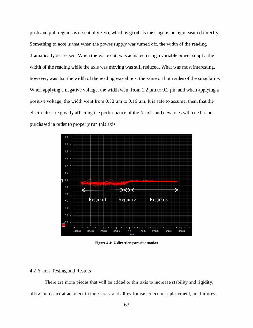
Preliminary testing has shown that the X-axis has at least a stiffness of 60 N/µm in both
the degrees of constraint. Movement in the parasitic directions while the axis was being actuated
was also tested and showed that the only movement in the parasitic directions is when the X-axis
crosses the zero point. Most likely, this is due to the electronics being used, which are also
making it difficult to determine the full range of the axis and close the loop. Testing on the Y-
axis has revealed that it has a stiffness of at least 125 N/µm in the direction of motion and
stiffnesses between 60 N/µm and 100 N/µm in the degrees of constraint. The axis is capable of
running at a speed of 150 µm/s, which is only limited by the amplifiers being used. Closed loop
testing has shown that the axis is capable of 10 nm steps.
Page 3
iii
TABLE OF CONTENTS
Chapter 1 : Introduction .................................................................................................................. 1
1.1 Motivation ............................................................................................................................. 1
1.2 Objectives ............................................................................................................................. 2
1.3 Approach and Scope of Thesis ............................................................................................. 4
1.4 Thesis Outline ....................................................................................................................... 6
Chapter 2 : Literature Review ......................................................................................................... 8
2.1 Lens Mold Manufacturing Methods ..................................................................................... 8
2.2 Single Point Diamond Turning ........................................................................................... 14
2.3 Limitations of Presented Technologies ............................................................................... 28
Chapter 3 : Machine Tool Development ....................................................................................... 29
3.1 Overview ............................................................................................................................. 29
3.2 Development of X-axis ....................................................................................................... 31
3.3 Development of Y-axis ....................................................................................................... 39
3.4 Development of Z-axis ....................................................................................................... 47
3.5 Summary ............................................................................................................................. 57
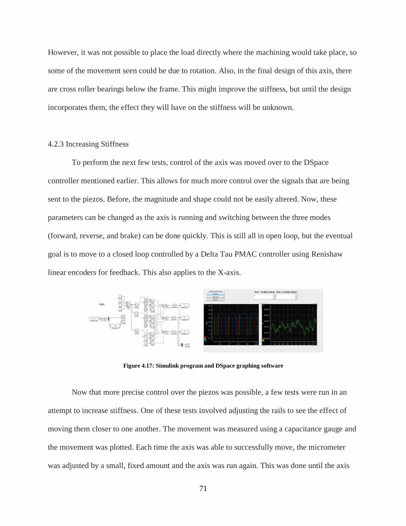
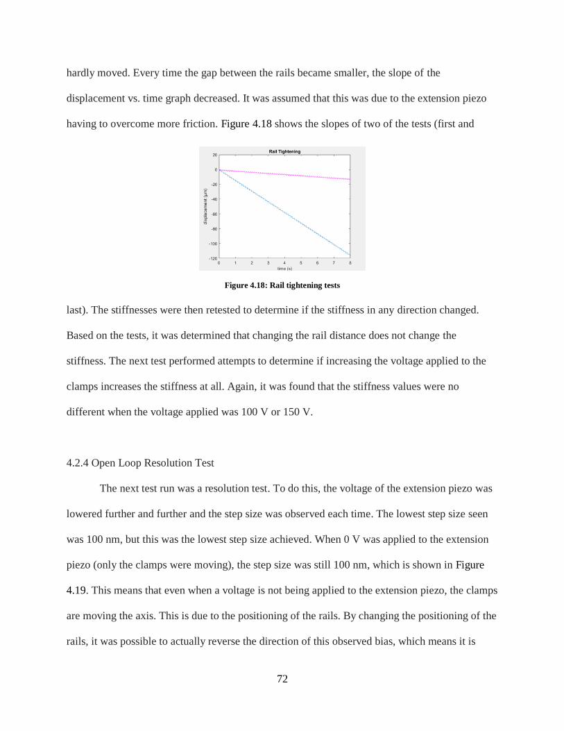
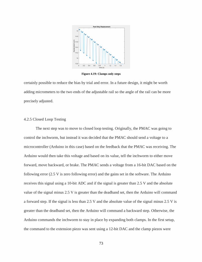
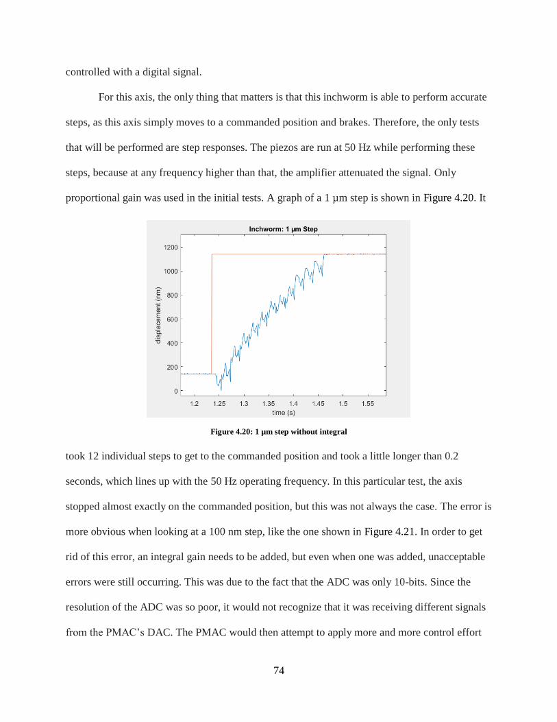
Chapter 4 : Testing and Results .................................................................................................... 59
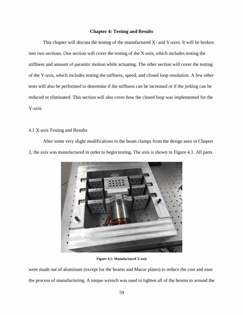
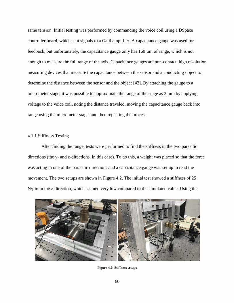
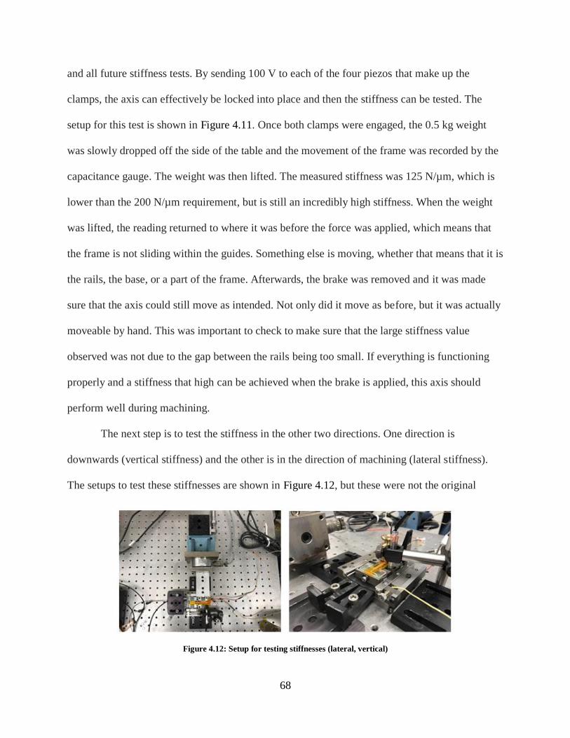
4.1 X-axis Testing and Results ................................................................................................. 59
4.2 Y-axis Testing and Results ................................................................................................. 63
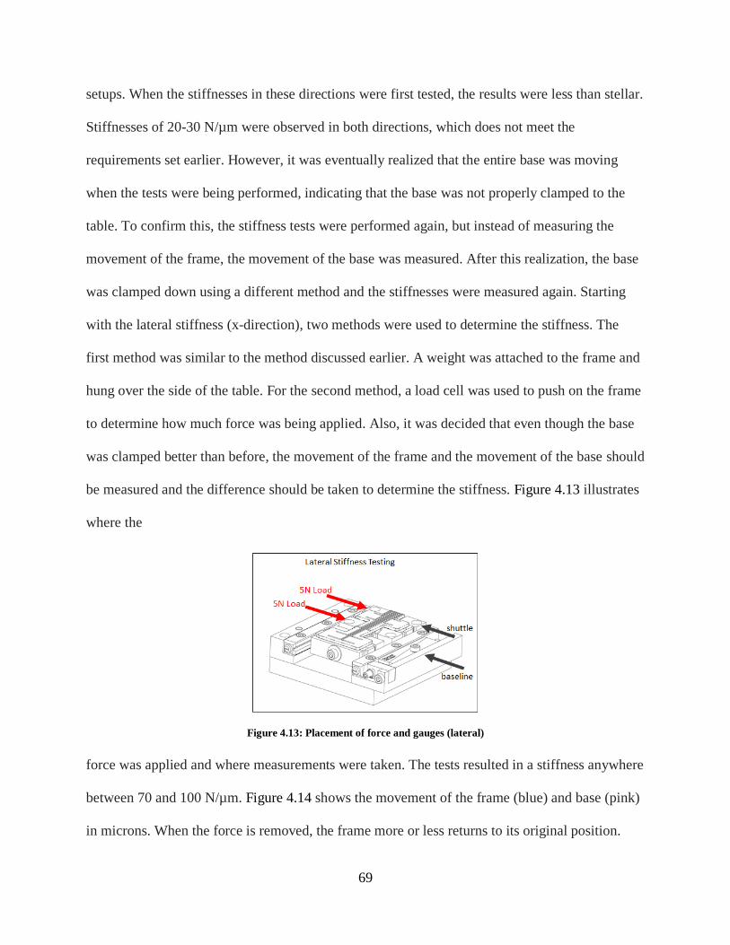
4.3 Summary ............................................................................................................................. 79
Chapter 5 : Conclusions and Future Work .................................................................................... 81
5.1 Conclusions ......................................................................................................................... 81
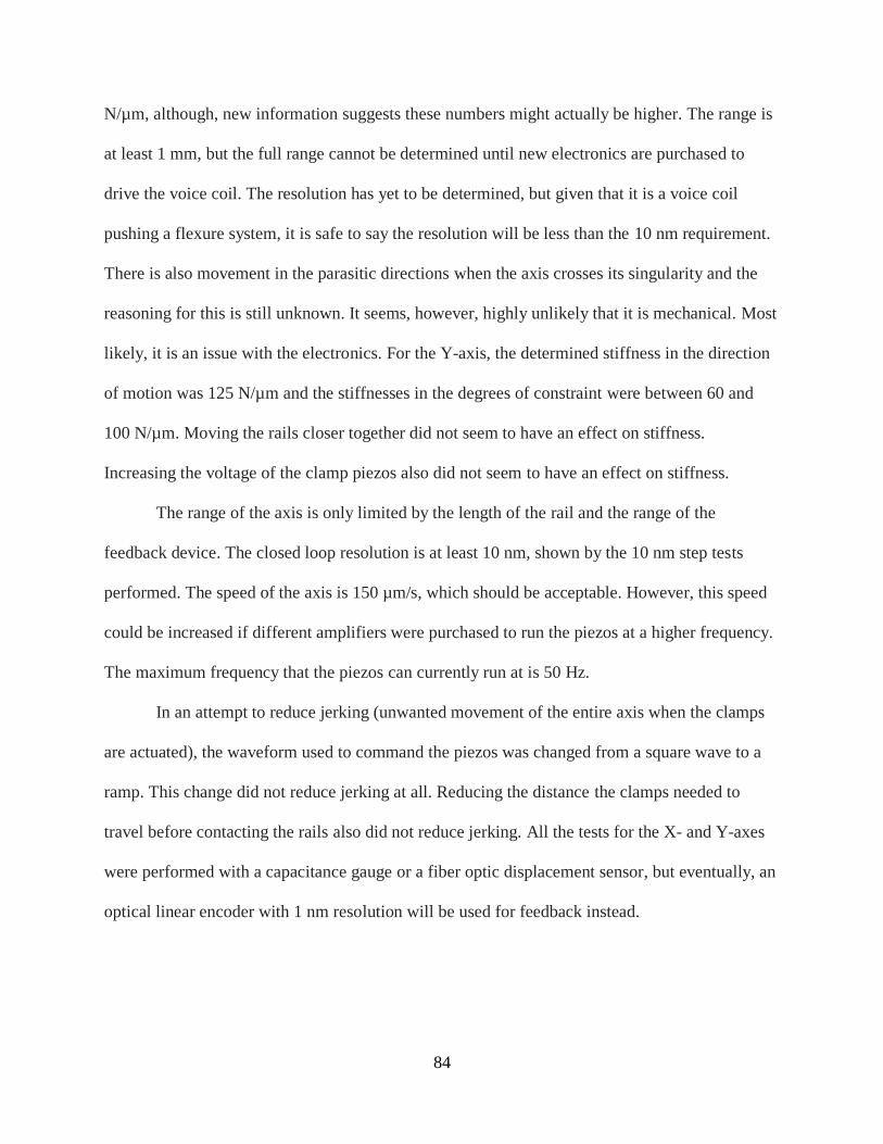
5.2 Future Work ........................................................................................................................ 85
References ..................................................................................................................................... 87
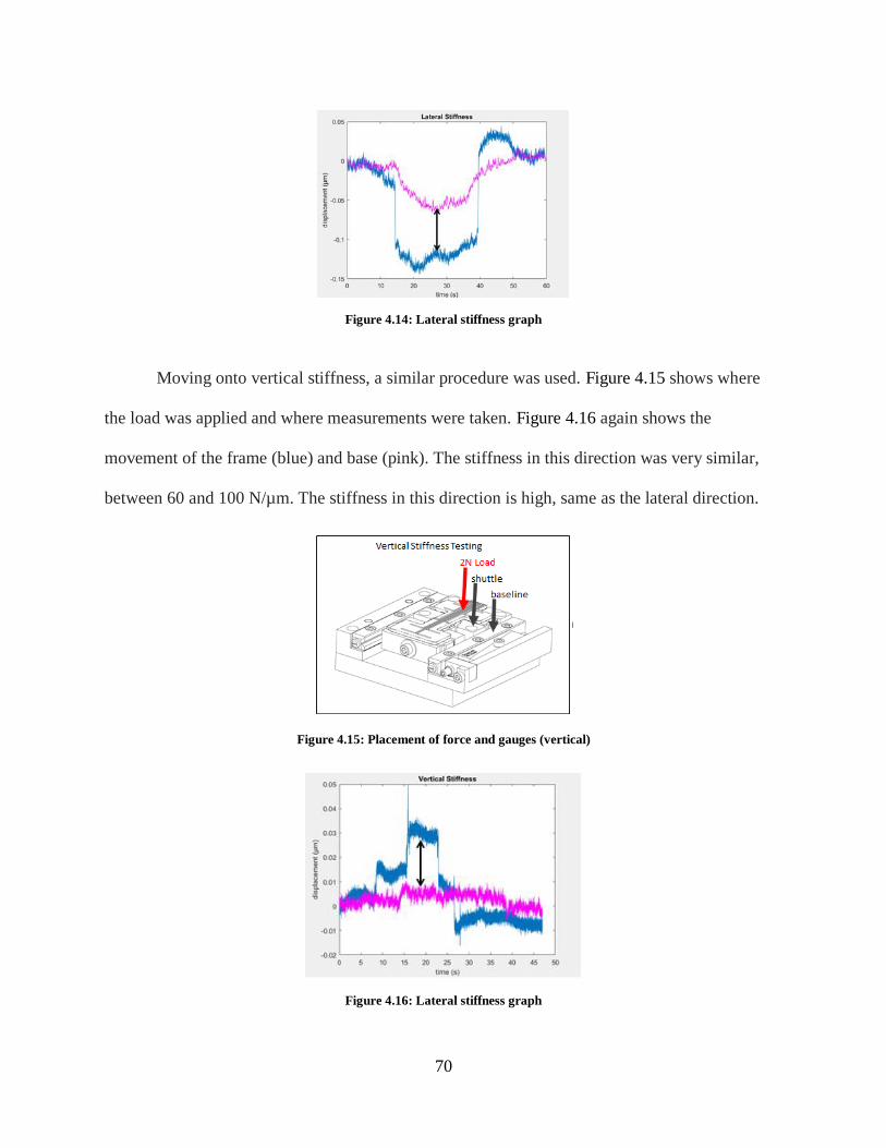
Page 4
1
Chapter 1: Introduction
1.1 Motivation
High-precision microlenses are seeing an increase in demand in many fields, including
laser communication, biological engineering, security monitoring, and national defense. They are
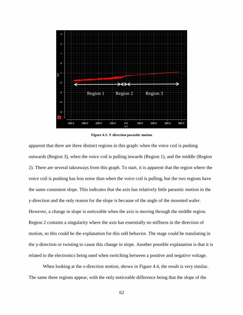
even being used in common, daily use items, such as phones and cameras [1], which are
currently being produced at rapid rates [2]. This overall growing need for microlenses has led to
the development and research of many different methods in order to produce them. Some of
these methods focus on fast production times, some focus on the fabrication of only spherical
lenses, and some focus on the ability to, albeit slowly, fabricate any type of microlens with
minimal errors. However, the ability to make high-precision freeform microlenses is generally
cost prohibitive, due to the expensive machines/components needed to machine these small,
complex surfaces with such strict form requirements.
The reason these machines are so costly is mainly due to the high resolution, accuracy,
and stiffness that each axis must have in order to produce accurate freeform microlens molds.
Surface roughness requirements for these molds are often less than 10 nm (Ra) and form
accuracy requirements are often less than 100 nm. On top of this, the most ideal metals to make
these molds from (e.g. stainless steel alloys) are generally difficult to machine. To meet the
requirements above, almost all of these machines use hydrostatic oil bearing slideways and
aerostatic air bearing spindles. Each of these axes has quite a high price tag, making the overall
machine an expensive purchase. Something else to note is that these machines might need
additional add-ons so they are capable of machining a specific microlens shape. For instance, it
might be necessary to add a fast tool servo (FTS) to the machine, as the provided Z-axis might
not have the acceleration needed to machine certain geometries. Commercial fast tool servos are
Page 5
2
even more expensive than any of the individual axes already discussed, which just adds to the
overall cost of building the machine. Therefore, there is a need for the development of a machine
that dramatically reduces the cost of producing freeform microlens molds with minimal form
error and low surface roughness.
1.2 Objectives
The primary objective of this research is to develop a relatively low cost, 3-axis
ultraprecision machine capable of machining an array of aspheric microlenses into a stainless
steel variant. In order to accomplish this, the following objectives must be completed:
1. X-, Y-, and Z-axes must be individually designed to meet certain criteria.
a. All three axes must have a resolution of 10 nm or less, high accuracy, high
repeatability, and stiffnesses of 200 N/µm in the necessary directions. Each axis
must be designed such that they will not experience fatigue failure due to high
stresses and will not heat up significantly during operation. The cost of creating
each axis should be a fraction of the cost of purchasing a commercial axis with
similar specifications.
b. The X-axis must have a range of motion greater than the width of one microlens.
c. The Y-axis must have a range of motion greater than the length of the entire
microlens array.
d. The Z-axis must have a range of motion greater than the depth of one microlens.
The Z-axis also must be capable of running at a frequency of at least 200 Hz at its
full range of motion.
2. Simulations must be performed on these axes to prove that they have the necessary range
Page 6
3
of motion and stiffness. These simulations also need to determine the stresses and
temperatures experienced by each axis when in operation.
3. Once an axis meets all the requirements set and it is shown that the cost of manufacturing
will be comparatively low to purchasing commercial components, parts will be purchased
and the axis will be manufactured.
4. Upon the completion of manufacturing an axis, tests will need to be performed to
determine if the manufactured axis is acceptable for ultraprecision machining. These
initial tests will include stiffness tests, resolution tests, and tests to determine the
movement in the parasitic directions.
5. A closed loop control system will need to be developed for each individual axis.
a. For the X-axis, the closed loop must be designed so that it can accurately follow a
sine wave command. This sine wave will likely not change during machining.
b. For the Y-axis, the closed loop must be designed so that it can accurately step to a
commanded position. Once it is within a certain range of that commanded
position, it will be commanded to lock into place. This is because the Y-axis acts
as a stepper axis.
c. For the Z-axis, the closed loop must be designed so that it can accurately follow
high frequency waveform commands. The profile this axis needs to follow will be
constantly changing in amplitude and frequency. The frequency of the Z-axis
commanded waveforms will be much higher than the X-axis commanded sine
waves, making control of this axis much more difficult.
Once each axis can be controlled separately, motion programs will need to be written in
order to control all three axes at once to accomplish the given task.
Page 7
4
6. The axes must be assembled into a machine and manufacturing of the aspheric microlens
mold can be attempted. Based on the results, adjustments to the machine will need to be
made until the desired product is achieved.
1.3 Approach and Scope of Thesis
In order to meet the objectives set above, specifically the first objective, it was
determined that each axis would need to be custom made, as the available commercial options
were far too expensive for this research. While this thesis will mainly focus on the X- and Y-
axes, as they have been not only been developed, but also manufactured and tested, the approach
to the development of all three axes is detailed below.
1.3.1 X-axis
In the machines discussed earlier, this axis is generally an aerostatic air bearing spindle.
However, it was determined that a linear axis would be easier and less expensive to custom
make. Since all three axes are linear, the machine being developed for this research is classified
as a shaper. Because the range of motion of this axis only needed to be the width of one lens,
which is less than 250 µm, it was decided that flexure bearings would be used for this axis.
Flexure bearings allow for compliance in one direction and are very stiff in the other directions.
To achieve the proper stiffness in the degrees of constraint, the flexures became quite difficult to
actuate in the direction of motion. To obtain the desired range of motion, a voice coil actuator
was used to actuate the axis, as it is capable of high forces, long ranges, and combined with the
flexure bearings, has basically unlimited resolution (only limited by the electronics). This axis
simply needs to follow an unchanging, low frequency sine wave when in closed loop (as
Page 8
5
discussed earlier), which should not be an issue for the voice coil. The reason this axis runs at
such a slow speed is because if the speed of this axis is increased, then the frequency the Z-axis
operates at would also need to be increased, making that axis more difficult to develop.
Simulations need to be performed and modifications need to be made until the simulations shows
that the X-axis has acceptable stiffness, range of motion, and stresses. Heat transfer simulations
will need to be performed as well. Once simulations are complete, the axis can then be
manufactured for testing.
1.3.2 Y-axis
While the X-axis is constantly moving back and forth, the Y-axis only needs to step to a
commanded position and hold that position until it is commanded to move again. However, the
range of this axis must be greater than the entire length of the microlens array, which is about 3
mm. Therefore, it was decided that an inchworm should be used for this axis, as inchworms have
unlimited range. This inchworm consists of two clamps and one extender. By actuating the
clamps and extender in a particular order, motion in either direction can be achieved. Five
piezoelectric actuators were used in the inchworm design (two for each clamp and one for the
extender), as the initial three piezo design did not meet the stiffness requirements. Piezos
produce high forces and have, again, theoretically unlimited resolution, which is why they were
chosen. A flexure frame was designed to hold the five piezos and simulations were performed on
the frame to ensure that stresses were not too high, the piezos would be capable of moving the
frame, and the stiffness requirements were met. The frame is placed between adjustable parallel
rails that are attached to a base, which will sit on top of the X-axis. The clamps will extend into
these rails. When the inchworm reaches a commanded position, both clamps will extend into the
Page 9
6
rails and lock the axis into place. Because piezos have such a large force output, the stiffness of
this axis in all directions when it is locked should be very high. Once it is determined that this
design will meet the requirements, the axis can be manufactured for testing.
1.3.3 Z-axis
As stated earlier, the Z-axis, which will be a fast tool servo, will need to actuate at 200
Hz at a range greater than 35 µm. Initially, the Z-axis was going to be designed similarly to the
X-axis, except a piezo would be used as the actuator instead of a voice coil. However, it was
decided that since the Z-axis will be much more difficult to control, it would make more sense to
design the axis to be a mechanism, which would make it linear, as opposed to the non-linear X-
axis. The frame that holds the piezo has flexure hinges that should make the frame very stiff in
the degrees of constraint, but the frame should still allow for a very strong piezo to move it in the
direction of motion. The piezo chosen is capable of actuating 60 µm at 400 Hz, but the preload
applied by the frame will limit the range a bit. Simulations and calculations will need to be
performed to determine if the axis has acceptable stiffness, range of motion, and stresses. The
resolution will only be limited by the electronics. The electronics to drive the piezo and the piezo
itself are expensive, which is partially why the axis has not yet been manufactured for testing.
However, the price of these two components is significantly less than a commercial FTS.
1.4 Thesis Outline
Chapter 2 presents a review of literature related to the manufacturing of lenses. The first
section reviews MEMS methods used to produce spherical microlenses. The second section
reviews the majority of ultraprecision machining methods used to produce lenses. The third
Page 10
7
section discusses the viability of the methods presented in the first two sections. The fourth
section reviews the remaining and most widely used ultraprecision machining method for the
creation of freeform microlenses: single point diamond turning.
Chapter 3 gives a detailed breakdown of the development of each of the three axes that
will be used in the final machine. First, though, an overview of the microlens array mold and
machine requirements is presented. The next three sections each discuss one axis by first laying
out the requirements for that axis and then presenting the step-by-step process on how that axis
was developed. This process includes coming up with an initial design, performing simulations
to determine stiffness, range of motion, stresses, heat generated, etc., and then modifying the
design until all the requirements are met.
Chapter 4 presents the manufactured X- and Y-axes. Each section details the testing
performed on one of the axes and the results of those tests. In these tests, stiffness, resolution,
range of motion, and parasitic movement will be determined. Once open loop testing has been
completed, a closed loop will be designed for each axis. With the current electronics being used
for the X-axis, there has been minimal success creating a closed loop that can follow a sine
wave. The Y-axis closed loop works well and tests to determine the speed and minimum step
size have been performed.
Chapter 5 presents conclusions of the completed work and discusses the future work that
needs to be done.
Page 11
8
Chapter 2: Literature Review
This chapter will discuss the aspects of lens and microlens mold manufacturing, as well
as existing technologies that could be used in the manufacturing of a microlens array mold. First,
the current techniques used for the manufacturing of lens and microlens molds will be reviewed,
followed by a discussion on the practicality of these methods for this research. Second, these
viable techniques and their associated technologies will be explored further. Finally, the
limitations of the reviewed technologies will be discussed.
2.1 Lens Mold Manufacturing Methods
Since lenses have such a wide range of applications, there have been several methods
developed for the formation of lenses of different sizes, shapes, and specifications. These
methods can be separated into two categories: direct and indirect. To put it simply, direct
methods do not require the fabrication of a mask or a mold to create the lens, while indirect
methods do [3]. This literature review will focus mainly on indirect methods, as it has already
been determined that direct methods will not be suitable for this research.
2.1.1 MEMS Methods
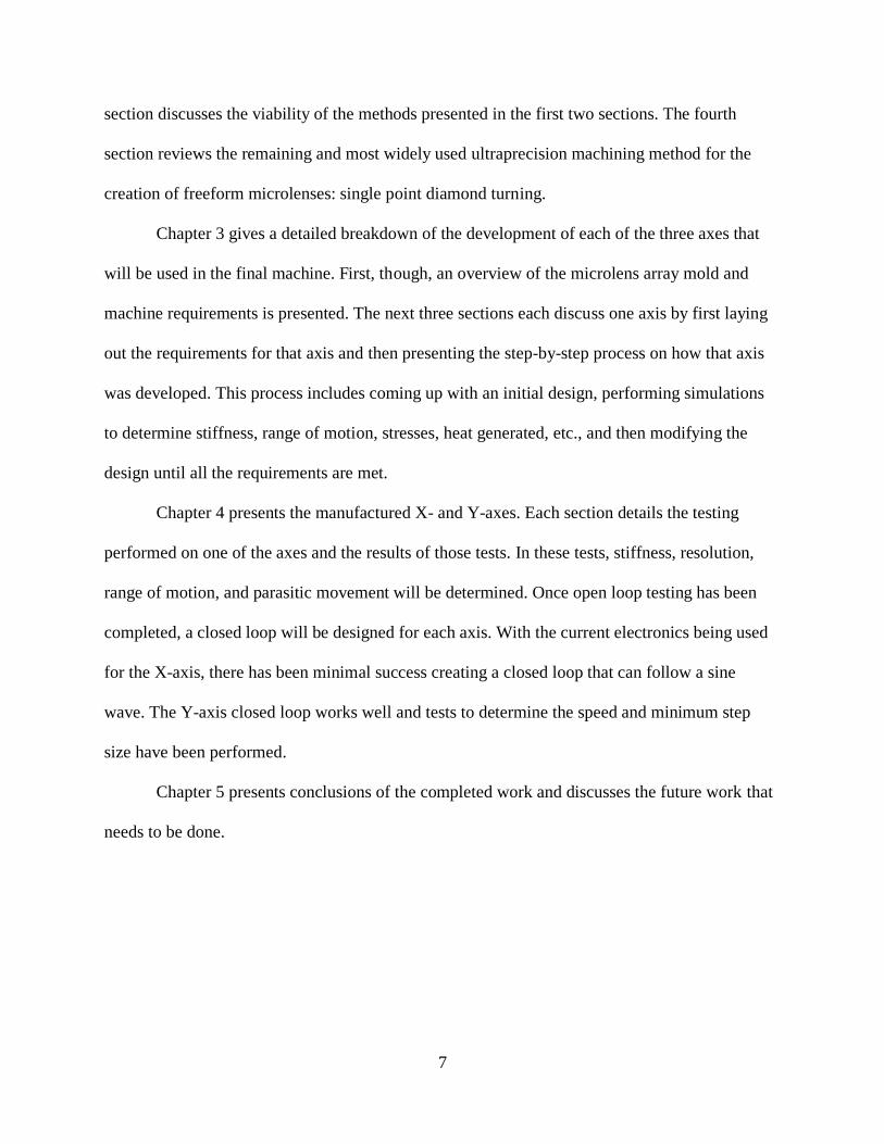
One of these methods, developed by Lin et al., uses UV proximity to create a mold in
photoresist. First, a mask is fabricated with the desired pattern. Photoresist is then spun onto the
substrate, which is a silicon wafer in this case. After alignment, exposure occurs for
approximately 8 seconds and then the array is developed for 2 minutes. PDMS is then cast onto
the photoresist and removed once it is cured. Figure 2.1 shows the flowchart of this process. This
method is used to produce spherical microlenses. While there is geometrical data on the
Page 12
9
produced arrays, the form error was not included. However, the surface roughness was measured
to be 2.31 nm [4].
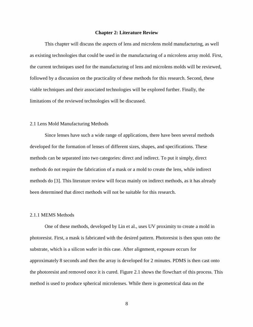
Another method, developed by Albero et al., also creates spherical microlenses, but
accomplishes it by using isotropic wet etching. To make the mold, a hard mask is first prepared
by adding layers of thermal oxide (SiO2), silicon nitride (Si3N4), and a nickel/chromium alloy
(NiCr) to a silicon wafer. The desired pattern is then produced using photolithography, reactive
ion etching (RIE), and an HF solution. After, the wafer is placed into an isotropic etch solution,
which forms the mold. When paired with agitation, the molds become more spherical, which is
desirable. This process is shown in Figure 2.2. The microlenses were created using either hot
embossing in combination with intermediate electroplated nickel foil shims or a UV-molding
process. The RMS wavefront deformation for a lens with a diameter of 230 µm (the largest lens
created in these experiments) was 5λ, while the measured surface roughness was 4-6 nm [5].
Figure 2.1: PDMS microlens array fabrication process [4]
Page 13
10
2.1.2 Ultraprecision Machining Methods
There are numerous ultraprecision machining methods that are used to manufacture lens
and microlens molds, including milling, grinding, and turning. Usually, these methods use
diamond tooling to perform the necessary machining, but there are other options available, which
will be covered later on.
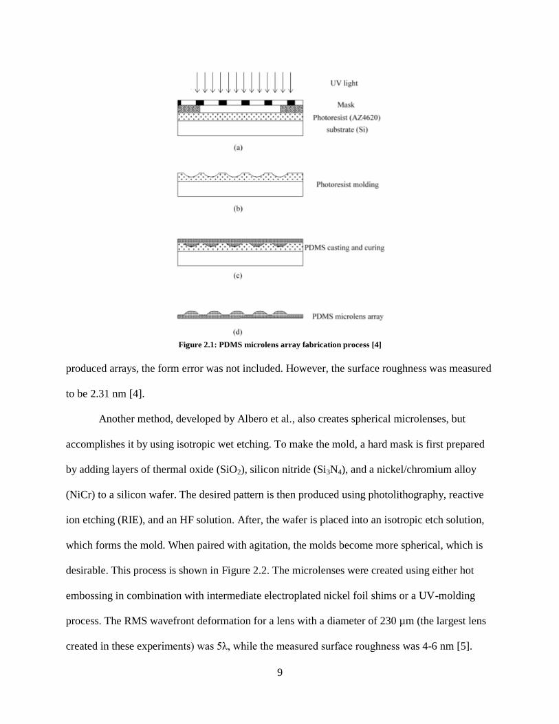
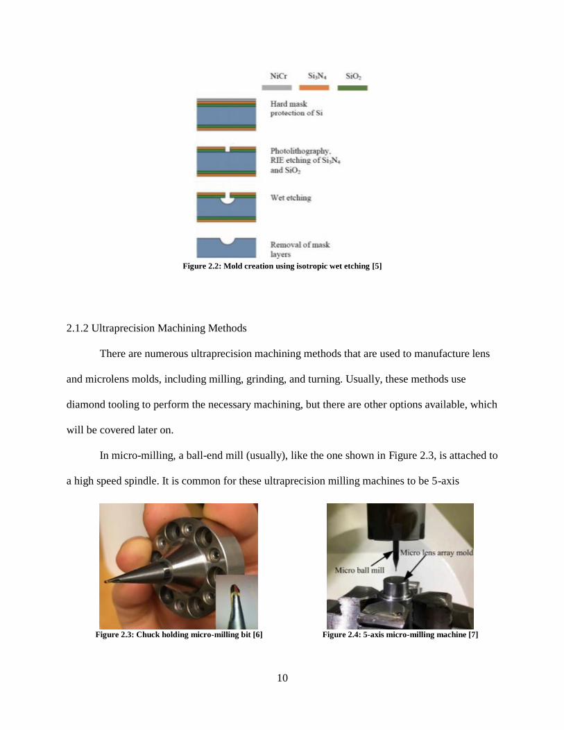
In micro-milling, a ball-end mill (usually), like the one shown in Figure 2.3, is attached to
a high speed spindle. It is common for these ultraprecision milling machines to be 5-axis
Figure 2.2: Mold creation using isotropic wet etching [5]
Figure 2.3: Chuck holding micro-milling bit [6]
Figure 2.4: 5-axis micro-milling machine [7]
Page 14
11
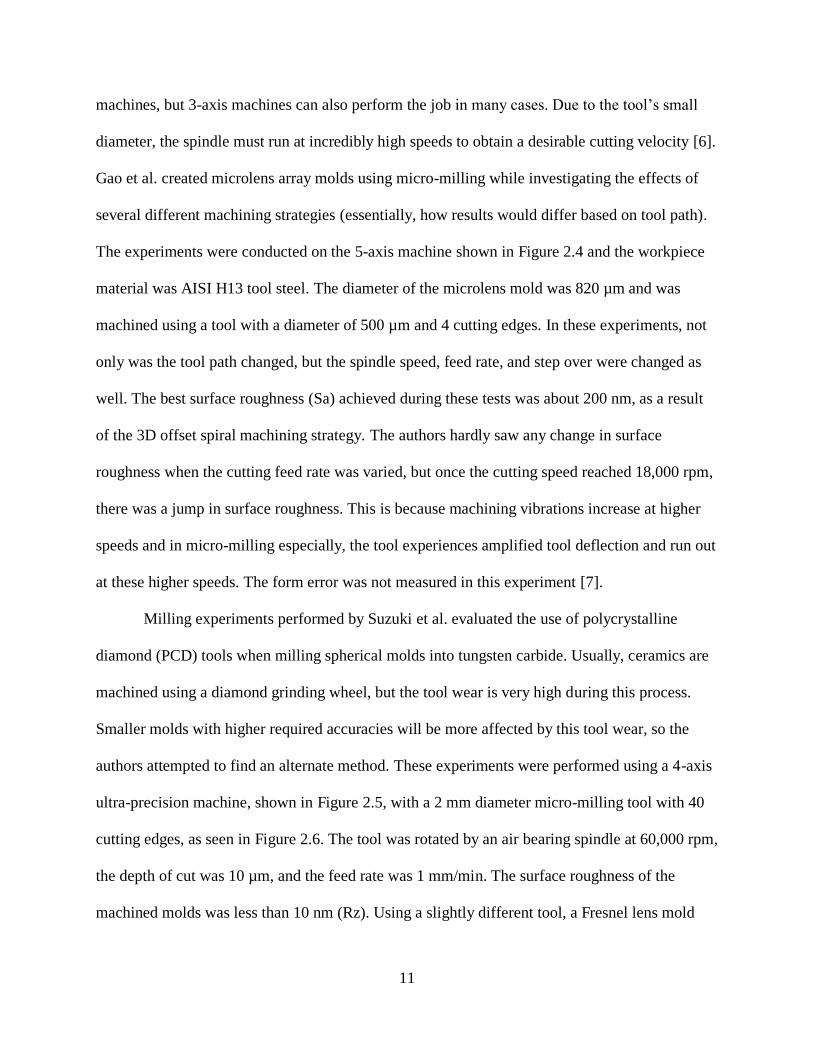
machines, but 3-axis machines can also perform the job in many cases. Due to the tool’s small
diameter, the spindle must run at incredibly high speeds to obtain a desirable cutting velocity [6].
Gao et al. created microlens array molds using micro-milling while investigating the effects of
several different machining strategies (essentially, how results would differ based on tool path).
The experiments were conducted on the 5-axis machine shown in Figure 2.4 and the workpiece
material was AISI H13 tool steel. The diameter of the microlens mold was 820 µm and was
machined using a tool with a diameter of 500 µm and 4 cutting edges. In these experiments, not
only was the tool path changed, but the spindle speed, feed rate, and step over were changed as
well. The best surface roughness (Sa) achieved during these tests was about 200 nm, as a result
of the 3D offset spiral machining strategy. The authors hardly saw any change in surface
roughness when the cutting feed rate was varied, but once the cutting speed reached 18,000 rpm,
there was a jump in surface roughness. This is because machining vibrations increase at higher
speeds and in micro-milling especially, the tool experiences amplified tool deflection and run out
at these higher speeds. The form error was not measured in this experiment [7].
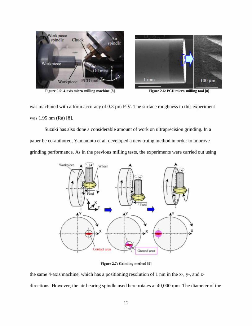
Milling experiments performed by Suzuki et al. evaluated the use of polycrystalline
diamond (PCD) tools when milling spherical molds into tungsten carbide. Usually, ceramics are
machined using a diamond grinding wheel, but the tool wear is very high during this process.
Smaller molds with higher required accuracies will be more affected by this tool wear, so the
authors attempted to find an alternate method. These experiments were performed using a 4-axis
ultra-precision machine, shown in Figure 2.5, with a 2 mm diameter micro-milling tool with 40
cutting edges, as seen in Figure 2.6. The tool was rotated by an air bearing spindle at 60,000 rpm,
the depth of cut was 10 µm, and the feed rate was 1 mm/min. The surface roughness of the
machined molds was less than 10 nm (Rz). Using a slightly different tool, a Fresnel lens mold
Page 15
12
was machined with a form accuracy of 0.3 µm P-V. The surface roughness in this experiment
was 1.95 nm (Ra) [8].
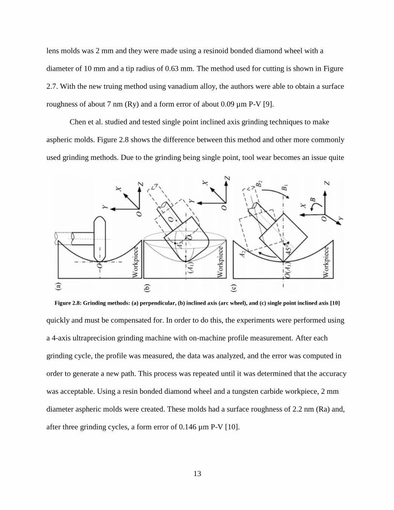
Suzuki has also done a considerable amount of work on ultraprecision grinding. In a
paper he co-authored, Yamamoto et al. developed a new truing method in order to improve
grinding performance. As in the previous milling tests, the experiments were carried out using
the same 4-axis machine, which has a positioning resolution of 1 nm in the x-, y-, and z-
directions. However, the air bearing spindle used here rotates at 40,000 rpm. The diameter of the
Figure 2.5: 4-axis micro-milling machine [8]
Figure 2.6: PCD micro-milling tool [8]
Figure 2.7: Grinding method [9]
Page 16
13
lens molds was 2 mm and they were made using a resinoid bonded diamond wheel with a
diameter of 10 mm and a tip radius of 0.63 mm. The method used for cutting is shown in Figure
2.7. With the new truing method using vanadium alloy, the authors were able to obtain a surface
roughness of about 7 nm (Ry) and a form error of about 0.09 µm P-V [9].
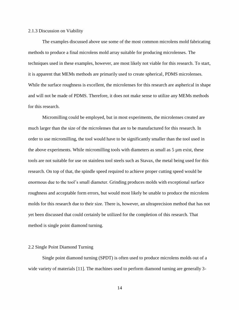
Chen et al. studied and tested single point inclined axis grinding techniques to make
aspheric molds. Figure 2.8 shows the difference between this method and other more commonly
used grinding methods. Due to the grinding being single point, tool wear becomes an issue quite
quickly and must be compensated for. In order to do this, the experiments were performed using
a 4-axis ultraprecision grinding machine with on-machine profile measurement. After each
grinding cycle, the profile was measured, the data was analyzed, and the error was computed in
order to generate a new path. This process was repeated until it was determined that the accuracy
was acceptable. Using a resin bonded diamond wheel and a tungsten carbide workpiece, 2 mm
diameter aspheric molds were created. These molds had a surface roughness of 2.2 nm (Ra) and,
after three grinding cycles, a form error of 0.146 µm P-V [10].
Figure 2.8: Grinding methods: (a) perpendicular, (b) inclined axis (arc wheel), and (c) single point inclined axis [10]
Page 17
14
2.1.3 Discussion on Viability
The examples discussed above use some of the most common microlens mold fabricating
methods to produce a final microlens mold array suitable for producing microlenses. The
techniques used in these examples, however, are most likely not viable for this research. To start,
it is apparent that MEMs methods are primarily used to create spherical, PDMS microlenses.
While the surface roughness is excellent, the microlenses for this research are aspherical in shape
and will not be made of PDMS. Therefore, it does not make sense to utilize any MEMs methods
for this research.
Micromilling could be employed, but in most experiments, the microlenses created are
much larger than the size of the microlenses that are to be manufactured for this research. In
order to use micromilling, the tool would have to be significantly smaller than the tool used in
the above experiments. While micromilling tools with diameters as small as 5 µm exist, these
tools are not suitable for use on stainless tool steels such as Stavax, the metal being used for this
research. On top of that, the spindle speed required to achieve proper cutting speed would be
enormous due to the tool’s small diameter. Grinding produces molds with exceptional surface
roughness and acceptable form errors, but would most likely be unable to produce the microlens
molds for this research due to their size. There is, however, an ultraprecision method that has not
yet been discussed that could certainly be utilized for the completion of this research. That
method is single point diamond turning.
2.2 Single Point Diamond Turning
Single point diamond turning (SPDT) is often used to produce microlens molds out of a
wide variety of materials [11]. The machines used to perform diamond turning are generally 3-
Page 18
15
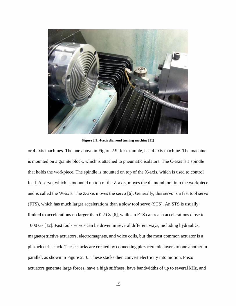
or 4-axis machines. The one above in Figure 2.9, for example, is a 4-axis machine. The machine
is mounted on a granite block, which is attached to pneumatic isolators. The C-axis is a spindle
that holds the workpiece. The spindle is mounted on top of the X-axis, which is used to control
feed. A servo, which is mounted on top of the Z-axis, moves the diamond tool into the workpiece
and is called the W-axis. The Z-axis moves the servo [6]. Generally, this servo is a fast tool servo
(FTS), which has much larger accelerations than a slow tool servo (STS). An STS is usually
limited to accelerations no larger than 0.2 Gs [6], while an FTS can reach accelerations close to
1000 Gs [12]. Fast tools servos can be driven in several different ways, including hydraulics,
magnetostrictive actuators, electromagnets, and voice coils, but the most common actuator is a
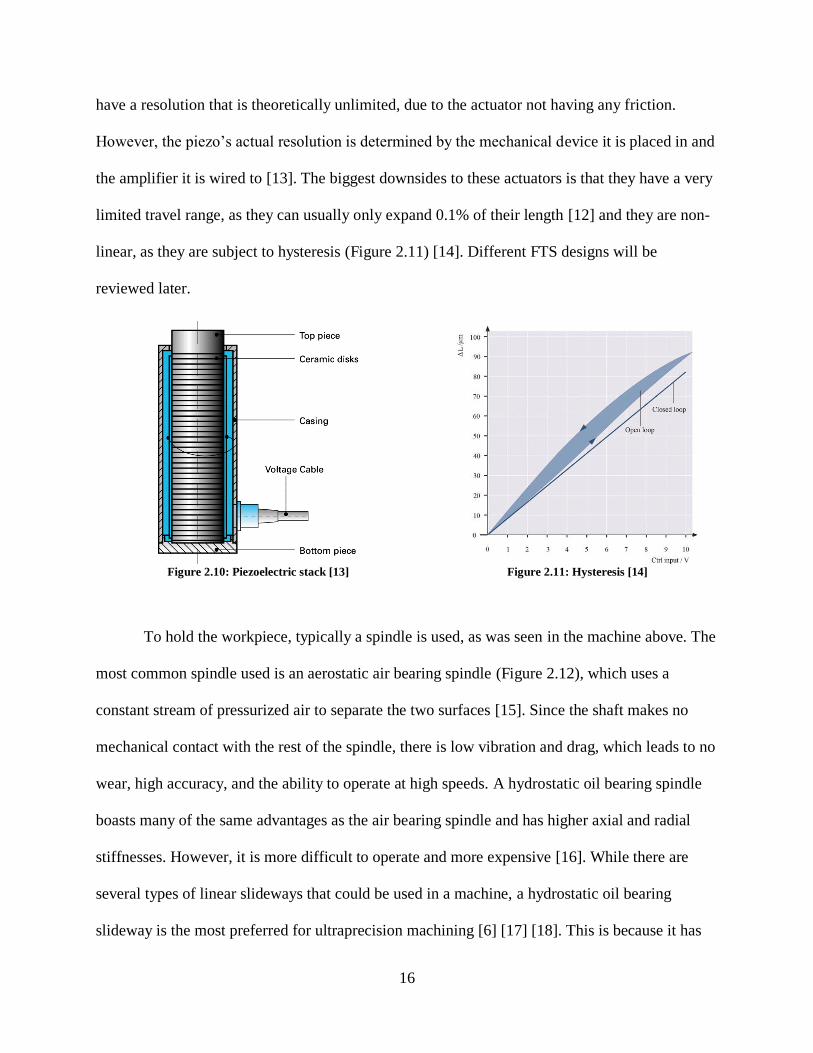
piezoelectric stack. These stacks are created by connecting piezoceramic layers to one another in
parallel, as shown in Figure 2.10. These stacks then convert electricity into motion. Piezo
actuators generate large forces, have a high stiffness, have bandwidths of up to several kHz, and
Figure 2.9: 4-axis diamond turning machine [11]
Page 19
16
have a resolution that is theoretically unlimited, due to the actuator not having any friction.
However, the piezo’s actual resolution is determined by the mechanical device it is placed in and
the amplifier it is wired to [13]. The biggest downsides to these actuators is that they have a very
limited travel range, as they can usually only expand 0.1% of their length [12] and they are non-
linear, as they are subject to hysteresis (Figure 2.11) [14]. Different FTS designs will be
reviewed later.
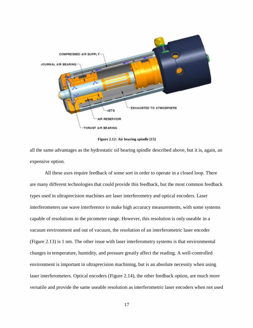
To hold the workpiece, typically a spindle is used, as was seen in the machine above. The
most common spindle used is an aerostatic air bearing spindle (Figure 2.12), which uses a
constant stream of pressurized air to separate the two surfaces [15]. Since the shaft makes no
mechanical contact with the rest of the spindle, there is low vibration and drag, which leads to no
wear, high accuracy, and the ability to operate at high speeds. A hydrostatic oil bearing spindle
boasts many of the same advantages as the air bearing spindle and has higher axial and radial
stiffnesses. However, it is more difficult to operate and more expensive [16]. While there are
several types of linear slideways that could be used in a machine, a hydrostatic oil bearing
slideway is the most preferred for ultraprecision machining [6] [17] [18]. This is because it has
Figure 2.10: Piezoelectric stack [13]
Figure 2.11: Hysteresis [14]
Page 20
17
all the same advantages as the hydrostatic oil bearing spindle described above, but it is, again, an
expensive option.
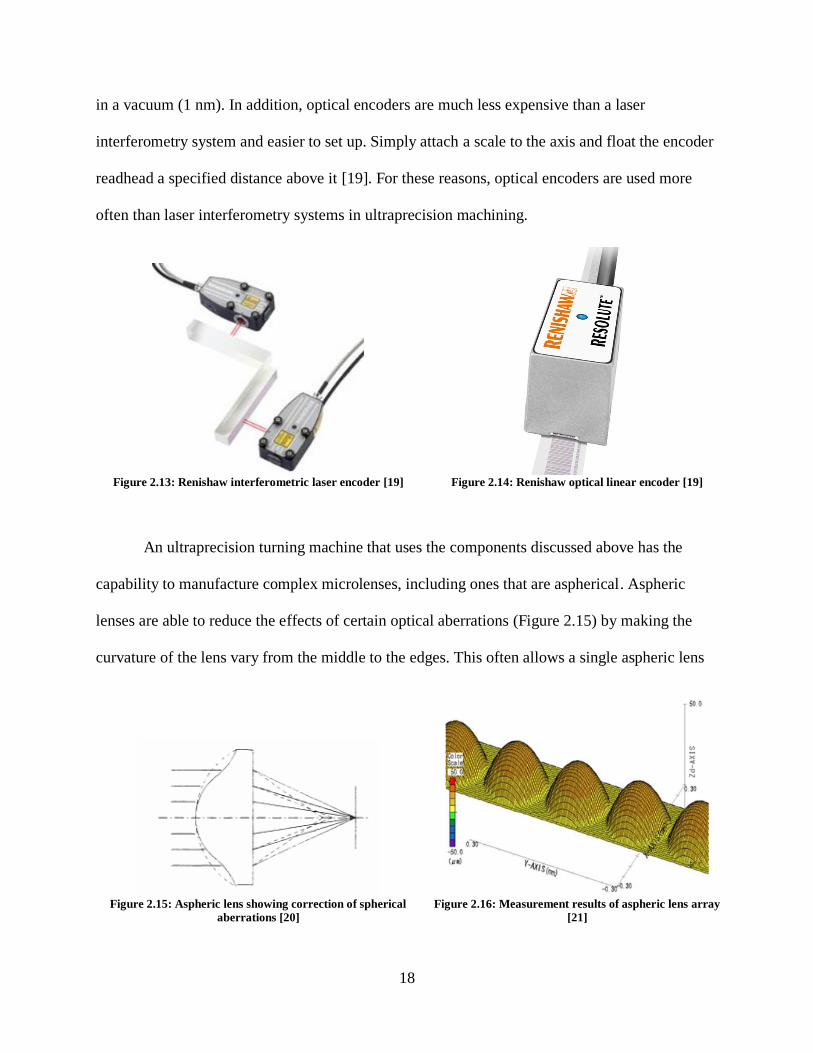
All these axes require feedback of some sort in order to operate in a closed loop. There
are many different technologies that could provide this feedback, but the most common feedback
types used in ultraprecision machines are laser interferometry and optical encoders. Laser
interferometers use wave interference to make high accuracy measurements, with some systems
capable of resolutions in the picometer range. However, this resolution is only useable in a
vacuum environment and out of vacuum, the resolution of an interferometric laser encoder
(Figure 2.13) is 1 nm. The other issue with laser interferometry systems is that environmental
changes in temperature, humidity, and pressure greatly affect the reading. A well-controlled
environment is important in ultraprecision machining, but is an absolute necessity when using
laser interferometers. Optical encoders (Figure 2.14), the other feedback option, are much more
versatile and provide the same useable resolution as interferometric laser encoders when not used
Figure 2.12: Air bearing spindle [15]
Page 21
18
in a vacuum (1 nm). In addition, optical encoders are much less expensive than a laser
interferometry system and easier to set up. Simply attach a scale to the axis and float the encoder
readhead a specified distance above it [19]. For these reasons, optical encoders are used more
often than laser interferometry systems in ultraprecision machining. [20] [21]
An ultraprecision turning machine that uses the components discussed above has the
capability to manufacture complex microlenses, including ones that are aspherical. Aspheric
lenses are able to reduce the effects of certain optical aberrations (Figure 2.15) by making the
curvature of the lens vary from the middle to the edges. This often allows a single aspheric lens
Figure 2.13: Renishaw interferometric laser encoder [19]
Figure 2.14: Renishaw optical linear encoder [19]
Figure 2.15: Aspheric lens showing correction of spherical
aberrations [20]
Figure 2.16: Measurement results of aspheric lens array
[21]
Page 22
19
to replace a system of multiple lenses, which saves space and reduces the weight of the device
using these lenses [22]. For some applications, a form error of 100 nm or less and a surface
roughness of 10 nm or less (Ra) are required. Form errors are usually specified as a peak-to-
valley error (P-V) and surface roughness is usually specified as a mean deviation from the
desired profile (Ra).
To achieve this form accuracy and surface finish, a single point diamond tool is usually
used. That is, if diamond tooling is appropriate for the workpiece material chosen. Diamond
tools work well on polymers and non-ferrous metals, but wear very quickly when cutting ferrous
metals (due to the iron in the metal), such as steel, and silicon [6]. This wear makes it difficult to
achieve the desired shape and surface finish, so it is necessary to find an alternative when
machining ferrous metals. One alternative is to use a cubic boron nitride (CBN) tool, which is
synthetically made and almost as hard. It is able to machine ferrous metals without significant
wear, but form error and surface finish will be higher compared to a diamond tool [6] [23].
Ultrasonic assisted diamond turning actually allows the use of a diamond tool on ferrous metals
and significantly reduces the wear experienced. This is accomplished by vibrating the tool at
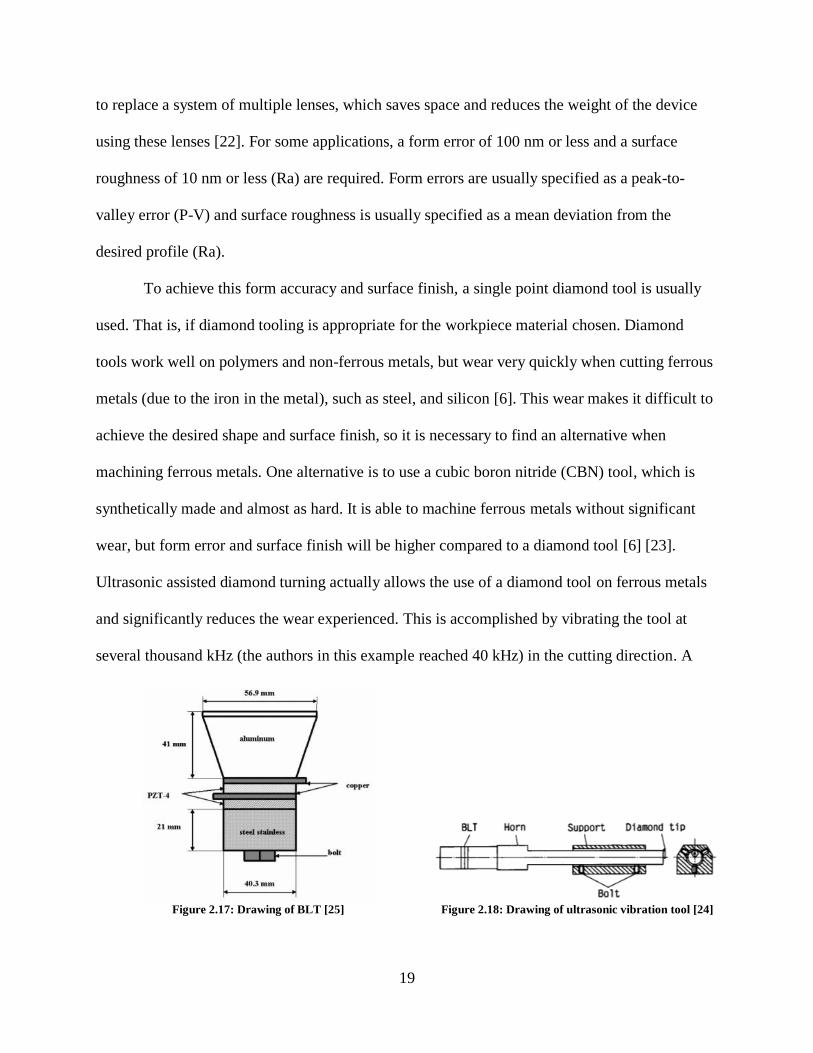
several thousand kHz (the authors in this example reached 40 kHz) in the cutting direction. A
Figure 2.17: Drawing of BLT [25]
Figure 2.18: Drawing of ultrasonic vibration tool [24]
Page 23
20
bolted Langevin transducer, shown in Figure 2.17, is used in conjunction with a horn (which
magnifies the vibration) in order to produce this vibration. An illustration of the entire setup is
shown in Figure 2.18. A surface roughness of 26 nm (Rmax) in stainless steel was obtained by the
authors in their experiments using ultrasonic assisted SPDT [24]. [25]
In another ultrasonically assisted SPDT experiment, Li et al. machined tungsten carbide
using a PCD tool and single crystal diamond tool and investigated the wear of the tool, the
surface roughness of the machined surface, and the efficiency of the process. The ultrasonic
vibration system was developed by the authors and used in conjunction with the Nanotech 250
ultraprecision lathe made by Moore Nanotechnology Systems [26]. This machine uses an air
bearing spindle to hold the workpiece and hydrostatic oil bearing box way slides for the X- and
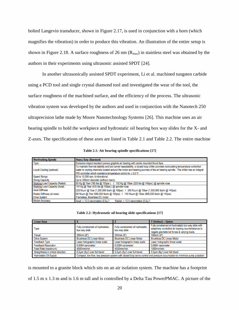
Z-axes. The specifications of these axes are listed in Table 2.1 and Table 2.2. The entire machine
is mounted to a granite block which sits on an air isolation system. The machine has a footprint
of 1.5 m x 1.3 m and is 1.6 m tall and is controlled by a Delta Tau PowerPMAC. A picture of the
Table 2.1: Air bearing spindle specifications [17]
Table 2.2: Hydrostatic oil bearing slide specifications [17]
Page 24
21
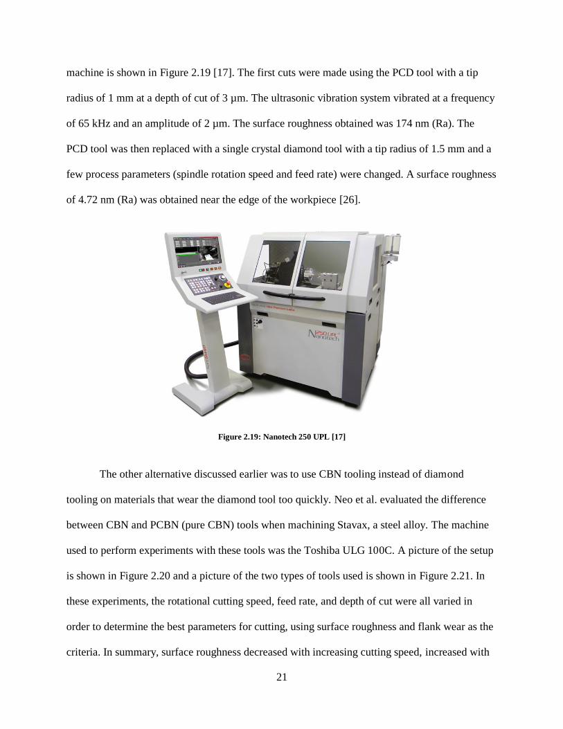
machine is shown in Figure 2.19 [17]. The first cuts were made using the PCD tool with a tip
radius of 1 mm at a depth of cut of 3 µm. The ultrasonic vibration system vibrated at a frequency
of 65 kHz and an amplitude of 2 µm. The surface roughness obtained was 174 nm (Ra). The
PCD tool was then replaced with a single crystal diamond tool with a tip radius of 1.5 mm and a
few process parameters (spindle rotation speed and feed rate) were changed. A surface roughness
of 4.72 nm (Ra) was obtained near the edge of the workpiece [26].
The other alternative discussed earlier was to use CBN tooling instead of diamond
tooling on materials that wear the diamond tool too quickly. Neo et al. evaluated the difference
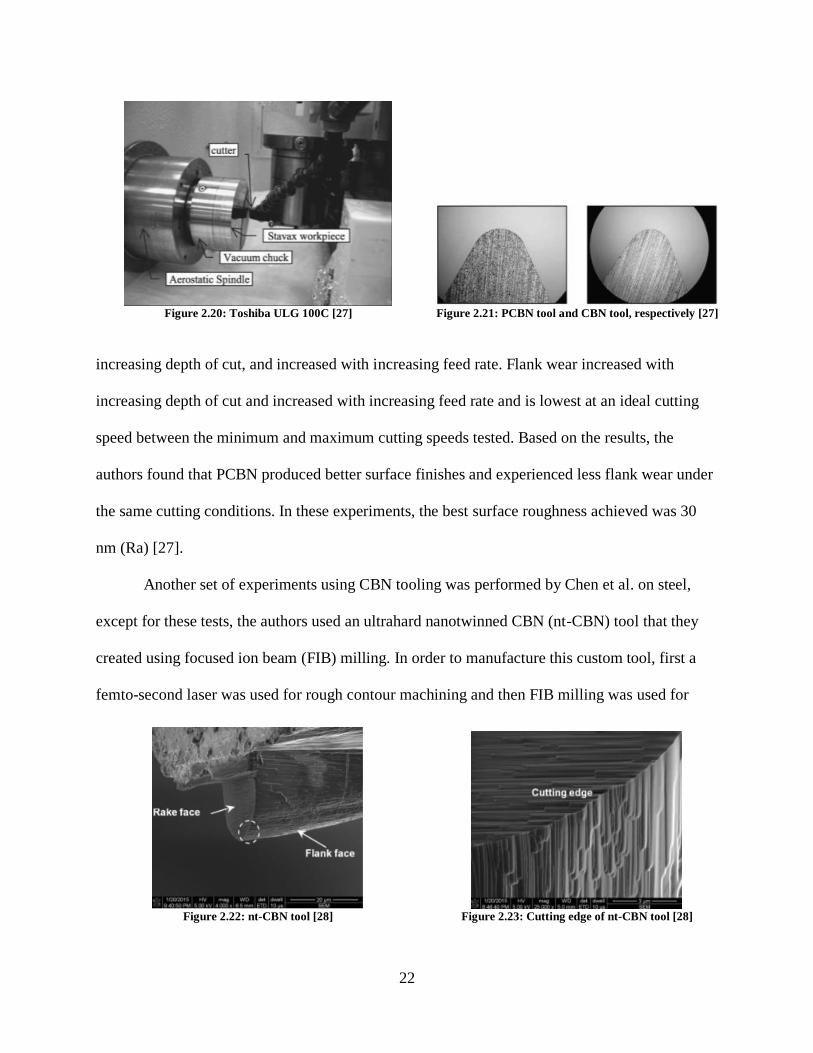
between CBN and PCBN (pure CBN) tools when machining Stavax, a steel alloy. The machine
used to perform experiments with these tools was the Toshiba ULG 100C. A picture of the setup
is shown in Figure 2.20 and a picture of the two types of tools used is shown in Figure 2.21. In
these experiments, the rotational cutting speed, feed rate, and depth of cut were all varied in
order to determine the best parameters for cutting, using surface roughness and flank wear as the
criteria. In summary, surface roughness decreased with increasing cutting speed, increased with
Figure 2.19: Nanotech 250 UPL [17]
Page 25
22
increasing depth of cut, and increased with increasing feed rate. Flank wear increased with
increasing depth of cut and increased with increasing feed rate and is lowest at an ideal cutting
speed between the minimum and maximum cutting speeds tested. Based on the results, the
authors found that PCBN produced better surface finishes and experienced less flank wear under
the same cutting conditions. In these experiments, the best surface roughness achieved was 30
nm (Ra) [27].
Another set of experiments using CBN tooling was performed by Chen et al. on steel,
except for these tests, the authors used an ultrahard nanotwinned CBN (nt-CBN) tool that they
created using focused ion beam (FIB) milling. In order to manufacture this custom tool, first a
femto-second laser was used for rough contour machining and then FIB milling was used for
Figure 2.20: Toshiba ULG 100C [27]
Figure 2.21: PCBN tool and CBN tool, respectively [27]
Figure 2.22: nt-CBN tool [28]
Figure 2.23: Cutting edge of nt-CBN tool [28]
Page 26
23
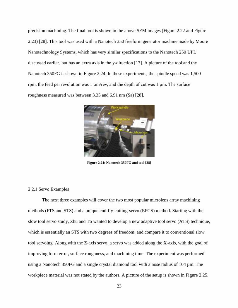
precision machining. The final tool is shown in the above SEM images (Figure 2.22 and Figure
2.23) [28]. This tool was used with a Nanotech 350 freeform generator machine made by Moore
Nanotechnology Systems, which has very similar specifications to the Nanotech 250 UPL
discussed earlier, but has an extra axis in the y-direction [17]. A picture of the tool and the
Nanotech 350FG is shown in Figure 2.24. In these experiments, the spindle speed was 1,500
rpm, the feed per revolution was 1 µm/rev, and the depth of cut was 1 µm. The surface
roughness measured was between 3.35 and 6.91 nm (Sa) [28].
2.2.1 Servo Examples
The next three examples will cover the two most popular microlens array machining
methods (FTS and STS) and a unique end-fly-cutting-servo (EFCS) method. Starting with the
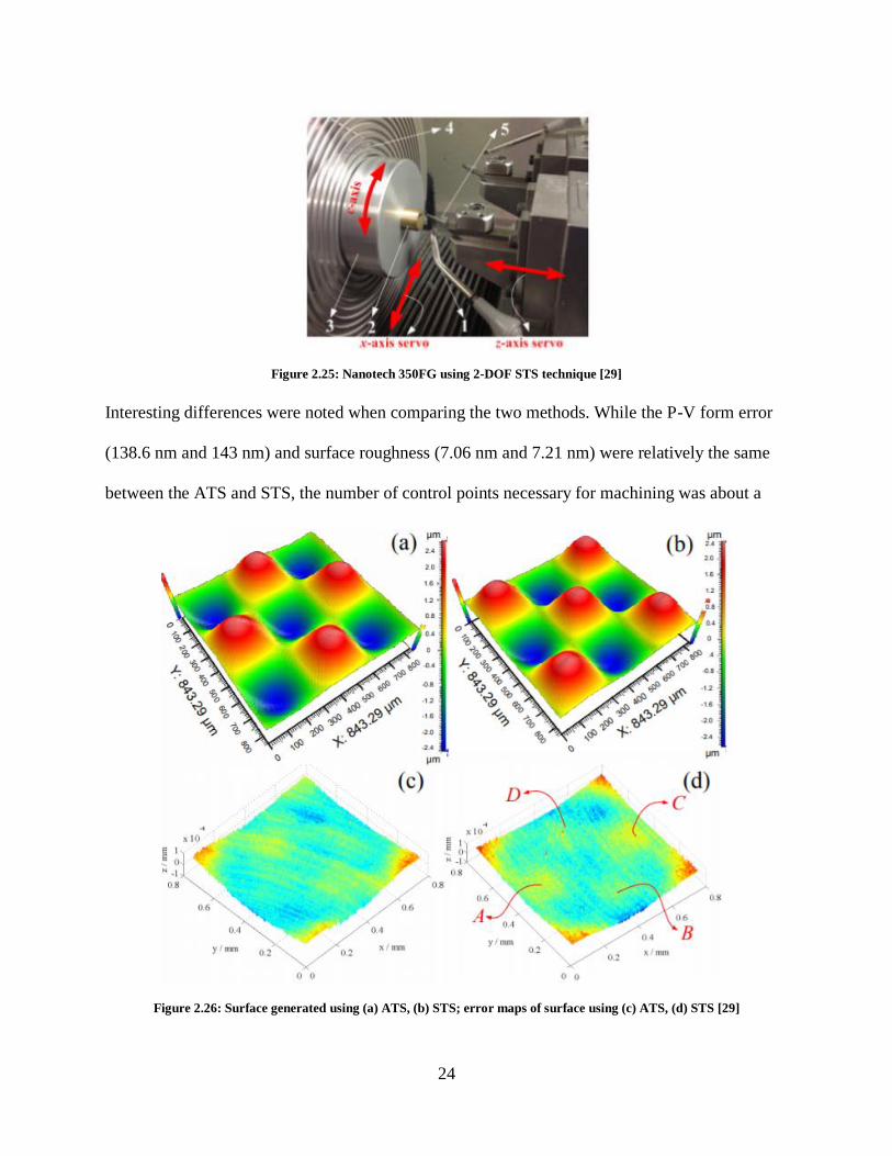
slow tool servo study, Zhu and To wanted to develop a new adaptive tool servo (ATS) technique,
which is essentially an STS with two degrees of freedom, and compare it to conventional slow
tool servoing. Along with the Z-axis servo, a servo was added along the X-axis, with the goal of
improving form error, surface roughness, and machining time. The experiment was performed
using a Nanotech 350FG and a single crystal diamond tool with a nose radius of 104 µm. The
workpiece material was not stated by the authors. A picture of the setup is shown in Figure 2.25.
Figure 2.24: Nanotech 350FG and tool [28]
Page 27
24
Interesting differences were noted when comparing the two methods. While the P-V form error
(138.6 nm and 143 nm) and surface roughness (7.06 nm and 7.21 nm) were relatively the same
between the ATS and STS, the number of control points necessary for machining was about a
Figure 2.25: Nanotech 350FG using 2-DOF STS technique [29]
Figure 2.26: Surface generated using (a) ATS, (b) STS; error maps of surface using (c) ATS, (d) STS [29]
Page 28
25
third less (383,000 vs. 600,000) and the machining time was also about a third less (1,412 sec vs.
2,105 sec). Graphs of the results are shown in Figure 2.26. The shape generated was a sinusoidal
grid. Based on these results, the authors concluded that the ATS method of machining could
produce similar results to the STS method, but in less time and using less control points, which is
important when machining certain optics, as the data set can sometimes be so large that the entire
process has to be slowed in order to transfer all of the data required [29].
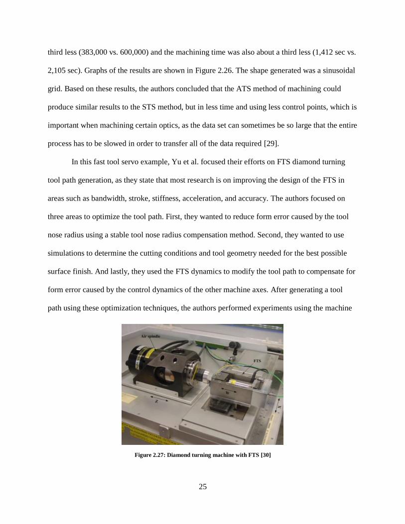
In this fast tool servo example, Yu et al. focused their efforts on FTS diamond turning
tool path generation, as they state that most research is on improving the design of the FTS in
areas such as bandwidth, stroke, stiffness, acceleration, and accuracy. The authors focused on
three areas to optimize the tool path. First, they wanted to reduce form error caused by the tool
nose radius using a stable tool nose radius compensation method. Second, they wanted to use
simulations to determine the cutting conditions and tool geometry needed for the best possible
surface finish. And lastly, they used the FTS dynamics to modify the tool path to compensate for
form error caused by the control dynamics of the other machine axes. After generating a tool
path using these optimization techniques, the authors performed experiments using the machine
Figure 2.27: Diamond turning machine with FTS [30]
Page 29
26
shown in Figure 2.27, which has the Z-axis under the air bearing spindle, the X-axis under the
FTS, and the FTS (called the W-axis), which actuates in the same direction as the Z-axis. In one
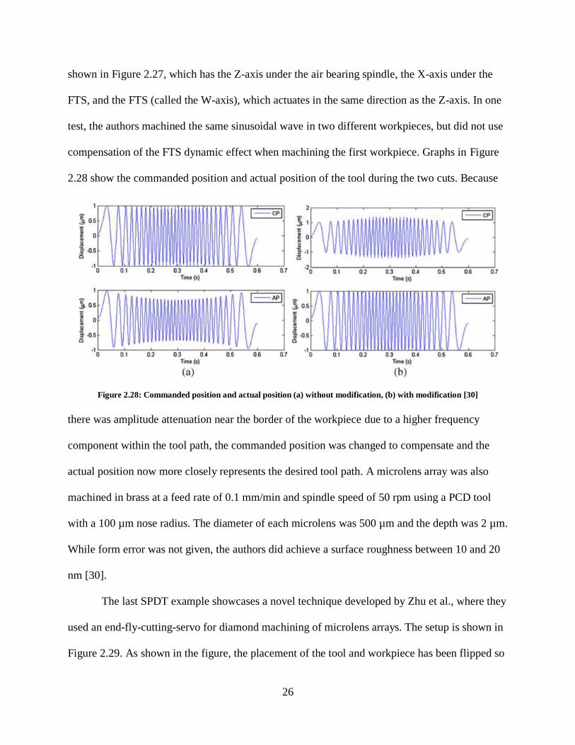
test, the authors machined the same sinusoidal wave in two different workpieces, but did not use
compensation of the FTS dynamic effect when machining the first workpiece. Graphs in Figure
2.28 show the commanded position and actual position of the tool during the two cuts. Because
there was amplitude attenuation near the border of the workpiece due to a higher frequency
component within the tool path, the commanded position was changed to compensate and the
actual position now more closely represents the desired tool path. A microlens array was also
machined in brass at a feed rate of 0.1 mm/min and spindle speed of 50 rpm using a PCD tool
with a 100 µm nose radius. The diameter of each microlens was 500 µm and the depth was 2 µm.
While form error was not given, the authors did achieve a surface roughness between 10 and 20
nm [30].
The last SPDT example showcases a novel technique developed by Zhu et al., where they
used an end-fly-cutting-servo for diamond machining of microlens arrays. The setup is shown in
Figure 2.29. As shown in the figure, the placement of the tool and workpiece has been flipped so
Figure 2.28: Commanded position and actual position (a) without modification, (b) with modification [30]
Page 30
27
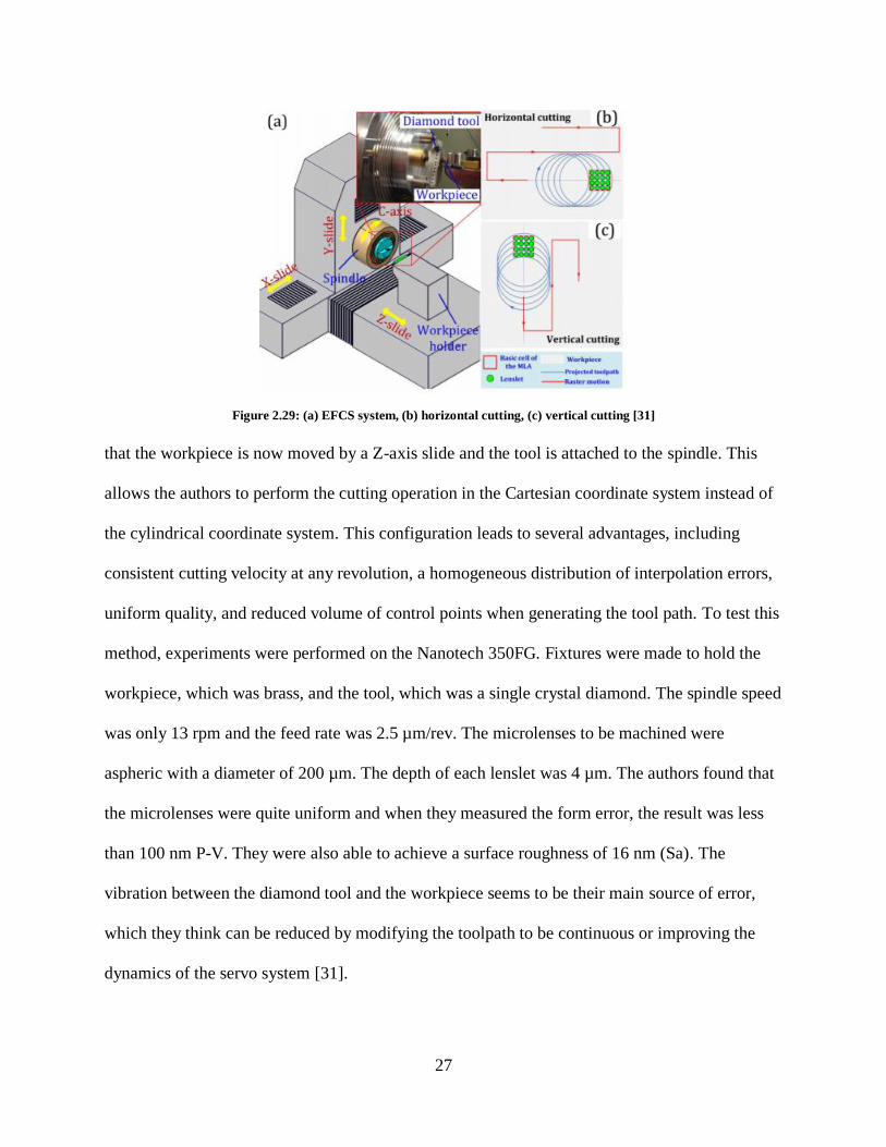
that the workpiece is now moved by a Z-axis slide and the tool is attached to the spindle. This
allows the authors to perform the cutting operation in the Cartesian coordinate system instead of
the cylindrical coordinate system. This configuration leads to several advantages, including
consistent cutting velocity at any revolution, a homogeneous distribution of interpolation errors,
uniform quality, and reduced volume of control points when generating the tool path. To test this
method, experiments were performed on the Nanotech 350FG. Fixtures were made to hold the
workpiece, which was brass, and the tool, which was a single crystal diamond. The spindle speed
was only 13 rpm and the feed rate was 2.5 µm/rev. The microlenses to be machined were
aspheric with a diameter of 200 µm. The depth of each lenslet was 4 µm. The authors found that
the microlenses were quite uniform and when they measured the form error, the result was less
than 100 nm P-V. They were also able to achieve a surface roughness of 16 nm (Sa). The
vibration between the diamond tool and the workpiece seems to be their main source of error,
which they think can be reduced by modifying the toolpath to be continuous or improving the
dynamics of the servo system [31].
Figure 2.29: (a) EFCS system, (b) horizontal cutting, (c) vertical cutting [31]
Page 31
28
2.3 Limitations of Presented Technologies
The two Moore Nanotechnology machines discussed above or the similarly built
ultraprecision machines that Precitech offers (Nanoform 700 ultra and Nanoform L 1000) can
most likely produce any type of lens mold, given the proper add-ons and modifications. The axes
have high stiffness, are capable of small resolutions, and have enough range, but these machines
are incredibly costly. When looking at the individual components, recall that the Moore
Nanotechnology machines used hydrostatic oil bearing slideways and an aerostatic air bearing
spindle. However, even buying the parts individually and assembling a machine with those parts
is not cost effective, especially if a commercial fast tool servo is added to the machine.
Page 32
29
Chapter 3: Machine Tool Development
This chapter will discuss the development of an ultraprecision machine that will be used
to create microlens molds from the stainless steel variant Stavax. This machine will need to meet
several specifications in order to satisfy the given form accuracy and surface roughness
requirements. Since the machine will consist of three axes, the chapter will be broken down into
four sections. The first section will give an overview of the microlens array mold requirements
and the overall machine specifications necessary to complete it. The next three sections will each
cover the development of one of the three axes, while also providing a breakdown of similar
technologies. Simulations will be performed to ensure that each of the axes meets the
requirements set in the first section.
3.1 Overview
The end goal of this research is to create a mold to be used for manufacturing aspheric
microlenses. The lens concave is less than 250 µm in diameter and less than 35 µm in depth. The
array consists of 12 lenses in a row with a spacing of approximately 11 µm. The workpiece is 0.6
mm by 4 mm and will be made out of pre-hardened Stavax. It was determined that machining
before hardening would not be possible, due to the changes the metal would undergo during the
hardening process. The workpiece will need to be faced beforehand, which can be done on
another machine if necessary. Based on the dimensions of the lens array, the machine will need a
working envelope of 3 mm by 0.25 mm by 0.035 mm, but it makes sense to design the machine
with a larger working envelope than the minimum dimensions of the lens array. The form error
must be less than 100 nm and the surface roughness must be less than 10 nm (Ra). In order to
meet these requirements: (1) the stiffness of the designed machine will need to be high (200
Page 33
30
N/µm) so that the tool does not move much during machining. Based on previous studies about
the machining of Stavax, it was determined that the maximum force that will likely occur during
machining would be about 10 N. If the stiffness is 200 N/µm, then the tool will only deflect 50
nm. 200 N/µm converted is slightly higher than 1,000,000 lbs/in, which is a high standard for the
stiffness of macro machines, (2) the resolution of each axis will need to be less than 10 nm, and
(3) the Z-axis will need to have a bandwidth of 200 Hz. A frequency decomposition of the lens
shape was performed and it was determined that to achieve maximum errors of 20 nm if the X-
axis is running at a speed of 1 mm/s, the Z-axis will have to actuate at 200 Hz.
Based on preliminary research work, it was decided that instead of a traditional spindle,
the X-axis will be a flexure-based, single DOF axis. Instead of a hydrostatic oil bearing slideway,
the Y-axis will be an inchworm axis. The Z-axis will be a fast tool servo. The machine will be
controlled by a Delta Tau Turbo PMAC motion controller and mounted on a granite block,
which will sit on pneumatic isolators. Custom making all three axes will not only drastically
reduce the cost of building the machine, but it also allows for customization of each axis to fit
the specifications outlined earlier. The axes will be discussed in the order that they were
developed.
In developing the ultraprecision machine, a custom spindle will not be made, but instead
replaced with another linear axis. This then turns the machine into a shaper, which is simply a
machine that has linear motion between the workpiece and tool. Using a shaper to generate
lenses provides a few advantages over a lathe, such as easier path generation, lens uniformity,
and efficiency if machining only one mold. The biggest disadvantage, however, is that the shaper
experiences constant large accelerations, while the spindle maintains a relatively constant
velocity.
Page 34
31
3.2 Development of X-axis
The X-axis will be a flexure-based, single DOF axis that will be mounted to the granite
block. Flexures are bearings that allow motion by bending (usually metal) beams. They are
generally very stiff in its degrees of constraint (DOC), but compliant in its degrees of freedom
(DOF). While the motion is limited, the movement is frictionless, which allows for a very
controllable motion [32]. The Y-axis will sit on top of X-axis and the Z-axis will hang above
from a gantry. This axis will be used to actuate along the shorter direction of the workpiece, so
the range of motion only needs to be as wide as one of the lenses. Therefore, this axis needs to be
designed such that the range of motion is greater than 250 µm, a resolution of less than 10 nm is
achievable, and the stiffness in the degrees of constraint is 200 N/µm.
3.2.1 Flexure Stage Examples
There are a multitude of flexure-based positioning stages that have been created, but the
majority of them do not have the range necessary for machining a microlens array. This is
because most of these stages use piezos as actuators. A different way to actuate a flexure stage
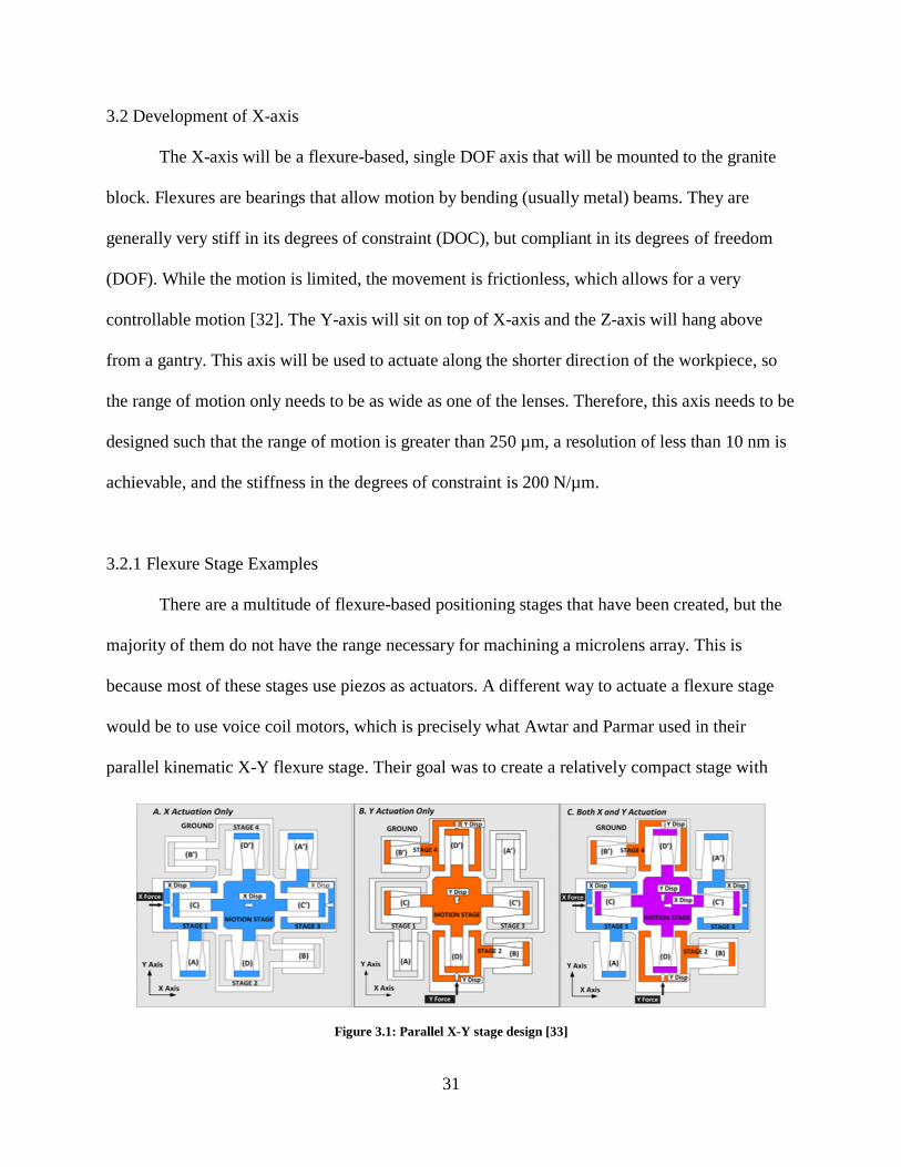
would be to use voice coil motors, which is precisely what Awtar and Parmar used in their
parallel kinematic X-Y flexure stage. Their goal was to create a relatively compact stage with
Figure 3.1: Parallel X-Y stage design [33]
Page 35
32
several millimeters of motion, while avoiding parasitic errors (movement in unactuated
directions) and decoupling the motion axes so that the motion of one axis did not significantly
affect the other axis’ motion. In order to accomplish this, the stage shown in Figure 3.1 was
proposed. Ideally, there should be no motion in the y-direction if only a force in the x-direction is
applied and vice-versa. However, in practice, there will probably be slight motion in the non-
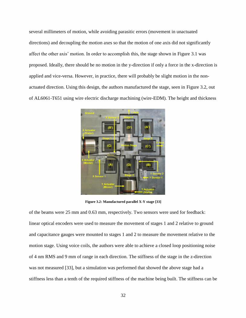
actuated direction. Using this design, the authors manufactured the stage, seen in Figure 3.2, out
of AL6061-T651 using wire electric discharge machining (wire-EDM). The height and thickness
of the beams were 25 mm and 0.63 mm, respectively. Two sensors were used for feedback:
linear optical encoders were used to measure the movement of stages 1 and 2 relative to ground
and capacitance gauges were mounted to stages 1 and 2 to measure the movement relative to the
motion stage. Using voice coils, the authors were able to achieve a closed loop positioning noise
of 4 nm RMS and 9 mm of range in each direction. The stiffness of the stage in the z-direction
was not measured [33], but a simulation was performed that showed the above stage had a
stiffness less than a tenth of the required stiffness of the machine being built. The stiffness can be
Figure 3.2: Manufactured parallel X-Y stage [33]
Page 36
33
increased using magnetic levitation bearings, using aerostatic bearings, or by increasing the
thickness and/or height of the leaf springs (beams) [34].
Long range, single DOF flexure stages have been researched as well, but not to the same
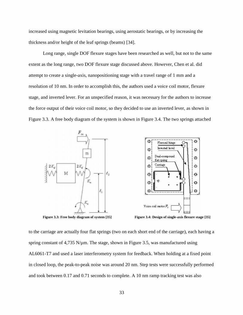
extent as the long range, two DOF flexure stage discussed above. However, Chen et al. did
attempt to create a single-axis, nanopositioning stage with a travel range of 1 mm and a
resolution of 10 nm. In order to accomplish this, the authors used a voice coil motor, flexure
stage, and inverted lever. For an unspecified reason, it was necessary for the authors to increase
the force output of their voice coil motor, so they decided to use an inverted lever, as shown in
Figure 3.3. A free body diagram of the system is shown in Figure 3.4. The two springs attached
to the carriage are actually four flat springs (two on each short end of the carriage), each having a
spring constant of 4,735 N/µm. The stage, shown in Figure 3.5, was manufactured using
AL6061-T7 and used a laser interferometry system for feedback. When holding at a fixed point
in closed loop, the peak-to-peak noise was around 20 nm. Step tests were successfully performed
and took between 0.17 and 0.71 seconds to complete. A 10 nm ramp tracking test was also
Figure 3.3: Free body diagram of system [35]
Figure 3.4: Design of single-axis flexure stage [35]
Page 37
34
successfully performed. Again, the parasitic stiffnesses were not measured [35].
3.2.2 Initial Design
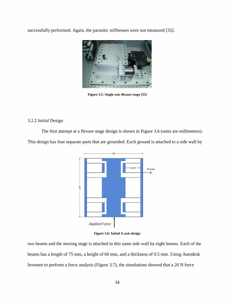
The first attempt at a flexure stage design is shown in Figure 3.6 (units are millimeters).
This design has four separate parts that are grounded. Each ground is attached to a side wall by
two beams and the moving stage is attached to this same side wall by eight beams. Each of the
beams has a length of 75 mm, a height of 60 mm, and a thickness of 0.5 mm. Using Autodesk
Inventor to perform a force analysis (Figure 3.7), the simulations showed that a 20 N force
Figure 3.5: Single-axis flexure stage [35]
Figure 3.6: Initial X-axis design
Page 38
35
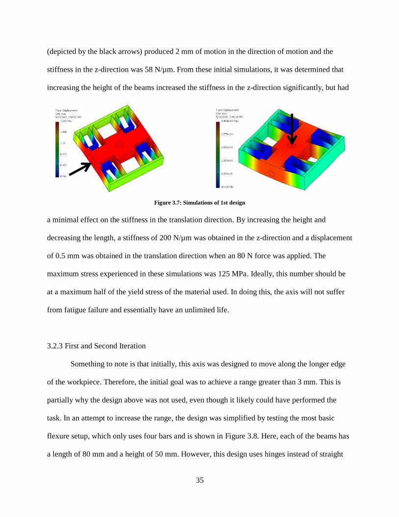
(depicted by the black arrows) produced 2 mm of motion in the direction of motion and the
stiffness in the z-direction was 58 N/µm. From these initial simulations, it was determined that
increasing the height of the beams increased the stiffness in the z-direction significantly, but had
a minimal effect on the stiffness in the translation direction. By increasing the height and
decreasing the length, a stiffness of 200 N/µm was obtained in the z-direction and a displacement
of 0.5 mm was obtained in the translation direction when an 80 N force was applied. The
maximum stress experienced in these simulations was 125 MPa. Ideally, this number should be
at a maximum half of the yield stress of the material used. In doing this, the axis will not suffer
from fatigue failure and essentially have an unlimited life.
3.2.3 First and Second Iteration
Something to note is that initially, this axis was designed to move along the longer edge
of the workpiece. Therefore, the initial goal was to achieve a range greater than 3 mm. This is
partially why the design above was not used, even though it likely could have performed the
task. In an attempt to increase the range, the design was simplified by testing the most basic
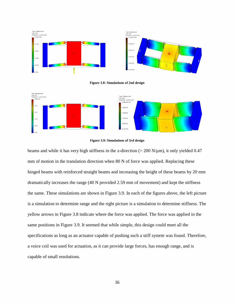
flexure setup, which only uses four bars and is shown in Figure 3.8. Here, each of the beams has
a length of 80 mm and a height of 50 mm. However, this design uses hinges instead of straight
Figure 3.7: Simulations of 1st design
Page 39
36
beams and while it has very high stiffness in the z-direction (> 200 N/µm), it only yielded 0.47
mm of motion in the translation direction when 80 N of force was applied. Replacing these
hinged beams with reinforced straight beams and increasing the height of these beams by 20 mm
dramatically increases the range (40 N provided 2.59 mm of movement) and kept the stiffness
the same. These simulations are shown in Figure 3.9. In each of the figures above, the left picture
is a simulation to determine range and the right picture is a simulation to determine stiffness. The
yellow arrows in Figure 3.8 indicate where the force was applied. The force was applied in the
same positions in Figure 3.9. It seemed that while simple, this design could meet all the
specifications as long as an actuator capable of pushing such a stiff system was found. Therefore,
a voice coil was used for actuation, as it can provide large forces, has enough range, and is
capable of small resolutions.
Figure 3.8: Simulations of 2nd design
Figure 3.9: Simulations of 3rd design
Page 40
37
3.2.4 Final Iteration
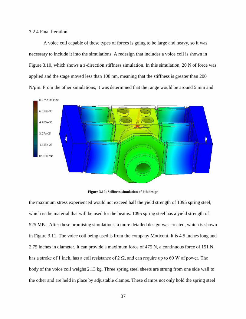
A voice coil capable of these types of forces is going to be large and heavy, so it was
necessary to include it into the simulations. A redesign that includes a voice coil is shown in
Figure 3.10, which shows a z-direction stiffness simulation. In this simulation, 20 N of force was
applied and the stage moved less than 100 nm, meaning that the stiffness is greater than 200
N/µm. From the other simulations, it was determined that the range would be around 5 mm and
the maximum stress experienced would not exceed half the yield strength of 1095 spring steel,
which is the material that will be used for the beams. 1095 spring steel has a yield strength of
525 MPa. After these promising simulations, a more detailed design was created, which is shown
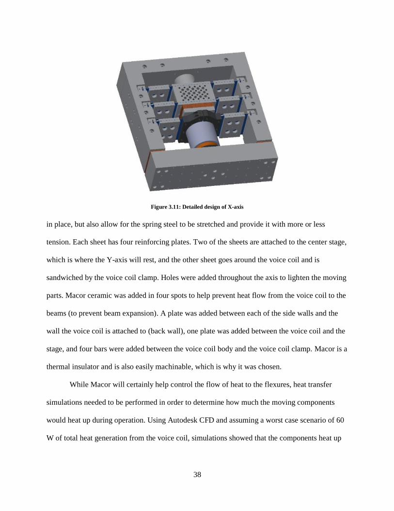
in Figure 3.11. The voice coil being used is from the company Moticont. It is 4.5 inches long and
2.75 inches in diameter. It can provide a maximum force of 475 N, a continuous force of 151 N,
has a stroke of 1 inch, has a coil resistance of 2 Ω, and can require up to 60 W of power. The
body of the voice coil weighs 2.13 kg. Three spring steel sheets are strung from one side wall to
the other and are held in place by adjustable clamps. These clamps not only hold the spring steel
Figure 3.10: Stiffness simulation of 4th design
Page 41
38
in place, but also allow for the spring steel to be stretched and provide it with more or less
tension. Each sheet has four reinforcing plates. Two of the sheets are attached to the center stage,
which is where the Y-axis will rest, and the other sheet goes around the voice coil and is
sandwiched by the voice coil clamp. Holes were added throughout the axis to lighten the moving
parts. Macor ceramic was added in four spots to help prevent heat flow from the voice coil to the
beams (to prevent beam expansion). A plate was added between each of the side walls and the
wall the voice coil is attached to (back wall), one plate was added between the voice coil and the
stage, and four bars were added between the voice coil body and the voice coil clamp. Macor is a
thermal insulator and is also easily machinable, which is why it was chosen.
While Macor will certainly help control the flow of heat to the flexures, heat transfer
simulations needed to be performed in order to determine how much the moving components
would heat up during operation. Using Autodesk CFD and assuming a worst case scenario of 60
W of total heat generation from the voice coil, simulations showed that the components heat up
Figure 3.11: Detailed design of X-axis
Page 42
39
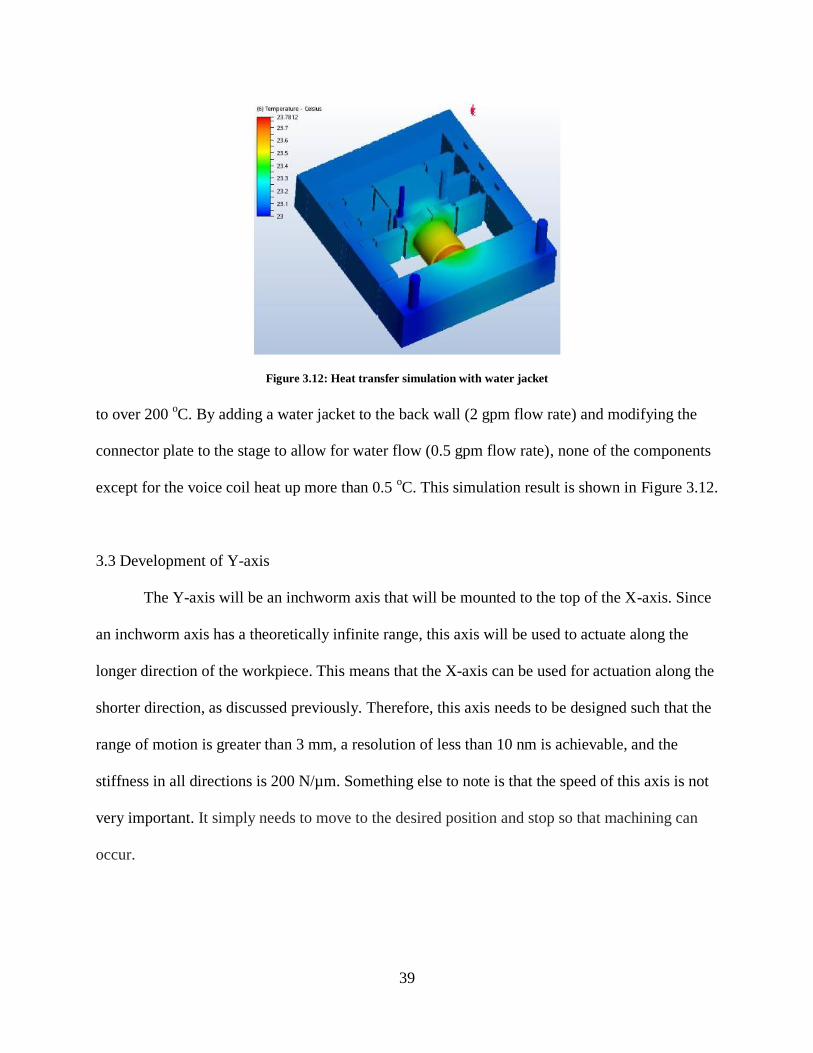
to over 200 oC. By adding a water jacket to the back wall (2 gpm flow rate) and modifying the
connector plate to the stage to allow for water flow (0.5 gpm flow rate), none of the components
except for the voice coil heat up more than 0.5 oC. This simulation result is shown in Figure 3.12.
3.3 Development of Y-axis
The Y-axis will be an inchworm axis that will be mounted to the top of the X-axis. Since
an inchworm axis has a theoretically infinite range, this axis will be used to actuate along the
longer direction of the workpiece. This means that the X-axis can be used for actuation along the
shorter direction, as discussed previously. Therefore, this axis needs to be designed such that the
range of motion is greater than 3 mm, a resolution of less than 10 nm is achievable, and the
stiffness in all directions is 200 N/µm. Something else to note is that the speed of this axis is not
very important. It simply needs to move to the desired position and stop so that machining can
occur.
Figure 3.12: Heat transfer simulation with water jacket
Page 43
40
3.3.1 Inchworm Examples
Inchworm actuators work by using clamps and a driver. In this example, there are two
clamps, which extend in a direction perpendicular to the desired direction of motion, which is the
direction the driver extends in. To produce movement, clamp 1 is locked into place by extending
into a wall, the driver extends, clamp 2 is locked, clamp 1 is unlocked, the driver contracts,
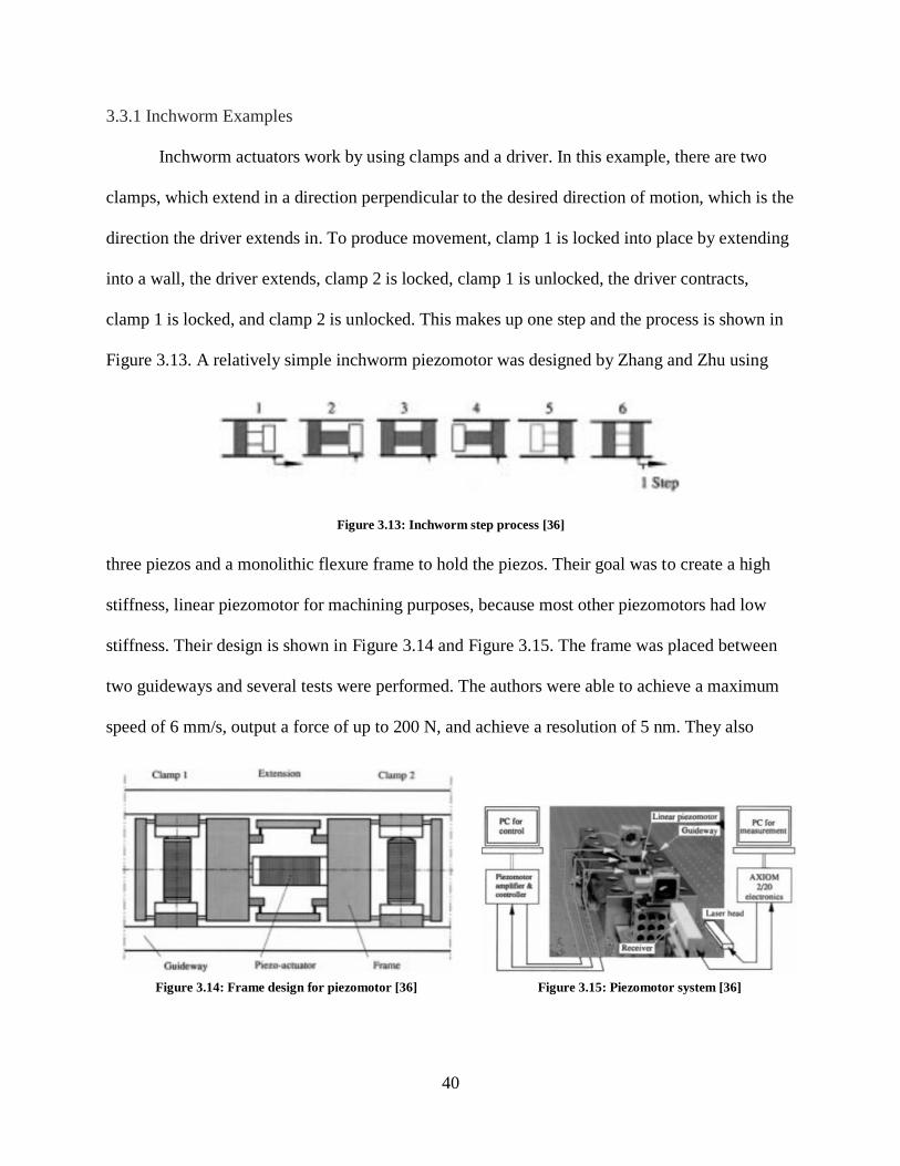
clamp 1 is locked, and clamp 2 is unlocked. This makes up one step and the process is shown in
Figure 3.13. A relatively simple inchworm piezomotor was designed by Zhang and Zhu using
three piezos and a monolithic flexure frame to hold the piezos. Their goal was to create a high
stiffness, linear piezomotor for machining purposes, because most other piezomotors had low
stiffness. Their design is shown in Figure 3.14 and Figure 3.15. The frame was placed between
two guideways and several tests were performed. The authors were able to achieve a maximum
speed of 6 mm/s, output a force of up to 200 N, and achieve a resolution of 5 nm. They also
Figure 3.13: Inchworm step process [36]
Figure 3.14: Frame design for piezomotor [36]
Figure 3.15: Piezomotor system [36]
Page 44
41
measured a stiffness of 90 N/µm in the travel direction. However, closed loop tests were not
performed and stiffnesses in the other directions were not given. They also experienced issues
with jerking, which is movement of the actuator in the direction of motion when the clamping
piezos engages the rails [36].
There are also several piezoelectric inchworm axes available to buy off-the-shelf from
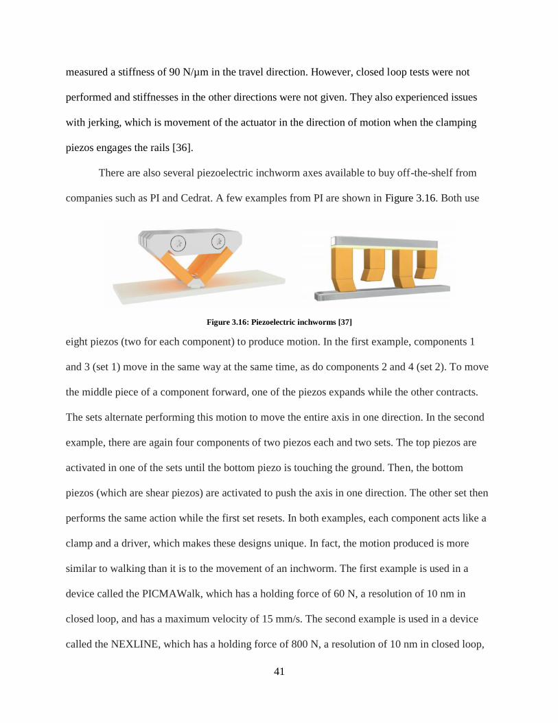
companies such as PI and Cedrat. A few examples from PI are shown in Figure 3.16. Both use
eight piezos (two for each component) to produce motion. In the first example, components 1
and 3 (set 1) move in the same way at the same time, as do components 2 and 4 (set 2). To move
the middle piece of a component forward, one of the piezos expands while the other contracts.
The sets alternate performing this motion to move the entire axis in one direction. In the second
example, there are again four components of two piezos each and two sets. The top piezos are
activated in one of the sets until the bottom piezo is touching the ground. Then, the bottom
piezos (which are shear piezos) are activated to push the axis in one direction. The other set then
performs the same action while the first set resets. In both examples, each component acts like a
clamp and a driver, which makes these designs unique. In fact, the motion produced is more
similar to walking than it is to the movement of an inchworm. The first example is used in a
device called the PICMAWalk, which has a holding force of 60 N, a resolution of 10 nm in
closed loop, and has a maximum velocity of 15 mm/s. The second example is used in a device
called the NEXLINE, which has a holding force of 800 N, a resolution of 10 nm in closed loop,
Figure 3.16: Piezoelectric inchworms [37]
Page 45
42
and has a maximum velocity 1 mm/s. Stiffnesses in the DOC are not given for either axis, but it
is not recommended to exceed 89 N in one of the DOC and 18 N in the other for the NEXLINE
actuator [37]. Both of these devices are quite expensive.
3.3.2 Initial Design
Since the price of these off-the-shelf inchworms is very high and they do not seem to
meet the necessary stiffness requirements, it was decided that a similar product would be
developed that had high stiffness in all directions. While the products above used eight piezos to
create movement, it was initially thought that this design would not need as many. These piezos
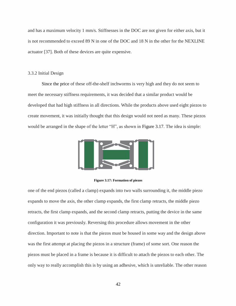
would be arranged in the shape of the letter “H”, as shown in Figure 3.17. The idea is simple:
one of the end piezos (called a clamp) expands into two walls surrounding it, the middle piezo
expands to move the axis, the other clamp expands, the first clamp retracts, the middle piezo
retracts, the first clamp expands, and the second clamp retracts, putting the device in the same
configuration it was previously. Reversing this procedure allows movement in the other
direction. Important to note is that the piezos must be housed in some way and the design above
was the first attempt at placing the piezos in a structure (frame) of some sort. One reason the
piezos must be placed in a frame is because it is difficult to attach the piezos to each other. The
only way to really accomplish this is by using an adhesive, which is unreliable. The other reason
Figure 3.17: Formation of piezos
Page 46
43
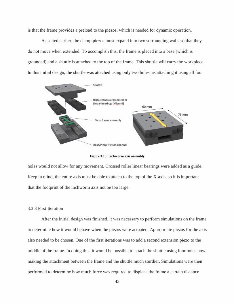
is that the frame provides a preload to the piezos, which is needed for dynamic operation.
As stated earlier, the clamp piezos must expand into two surrounding walls so that they
do not move when extended. To accomplish this, the frame is placed into a base (which is
grounded) and a shuttle is attached to the top of the frame. This shuttle will carry the workpiece.
In this initial design, the shuttle was attached using only two holes, as attaching it using all four
holes would not allow for any movement. Crossed roller linear bearings were added as a guide.
Keep in mind, the entire axis must be able to attach to the top of the X-axis, so it is important
that the footprint of the inchworm axis not be too large.
3.3.3 First Iteration
After the initial design was finished, it was necessary to perform simulations on the frame
to determine how it would behave when the piezos were actuated. Appropriate piezos for the axis
also needed to be chosen. One of the first iterations was to add a second extension piezo to the
middle of the frame. In doing this, it would be possible to attach the shuttle using four holes now,
making the attachment between the frame and the shuttle much sturdier. Simulations were then
performed to determine how much force was required to displace the frame a certain distance
Figure 3.18: Inchworm axis assembly
Page 47
44
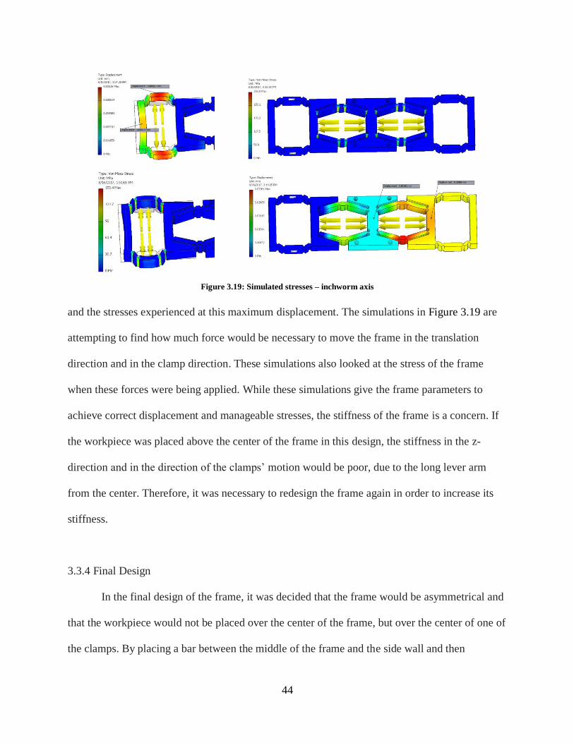
and the stresses experienced at this maximum displacement. The simulations in Figure 3.19 are
attempting to find how much force would be necessary to move the frame in the translation
direction and in the clamp direction. These simulations also looked at the stress of the frame
when these forces were being applied. While these simulations give the frame parameters to
achieve correct displacement and manageable stresses, the stiffness of the frame is a concern. If
the workpiece was placed above the center of the frame in this design, the stiffness in the z-
direction and in the direction of the clamps’ motion would be poor, due to the long lever arm
from the center. Therefore, it was necessary to redesign the frame again in order to increase its
stiffness.
3.3.4 Final Design
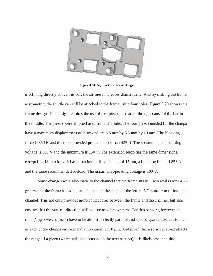
In the final design of the frame, it was decided that the frame would be asymmetrical and
that the workpiece would not be placed over the center of the frame, but over the center of one of
the clamps. By placing a bar between the middle of the frame and the side wall and then
Figure 3.19: Simulated stresses – inchworm axis
Page 48
45
machining directly above this bar, the stiffness increases dramatically. And by making the frame
asymmetric, the shuttle can still be attached to the frame using four holes. Figure 3.20 shows this
frame design. This design requires the use of five piezos instead of three, because of the bar in
the middle. The piezos were all purchased from Thorlabs. The four piezos needed for the clamps
have a maximum displacement of 9 µm and are 6.5 mm by 6.5 mm by 10 mm. The blocking
force is 850 N and the recommended preload is less than 425 N. The recommended operating
voltage is 100 V and the maximum is 150 V. The extension piezo has the same dimensions,
except it is 18 mm long. It has a maximum displacement of 15 µm, a blocking force of 853 N,
and the same recommended preload. The maximum operating voltage is 100 V.
Some changes were also made to the channel that the frame sits in. Each wall is now a V-
groove and the frame has added attachments in the shape of the letter “V” in order to fit into this
channel. This not only provides more contact area between the frame and the channel, but also
ensures that the vertical direction will not see much movement. For this to work, however, the
rails (V-groove channels) have to be almost perfectly parallel and spaced apart an exact distance,
as each of the clamps only expand a maximum of 18 µm. And given that a spring preload affects
the range of a piezo (which will be discussed in the next section), it is likely less than that.
Figure 3.20: Asymmetrical frame design
Page 49
46
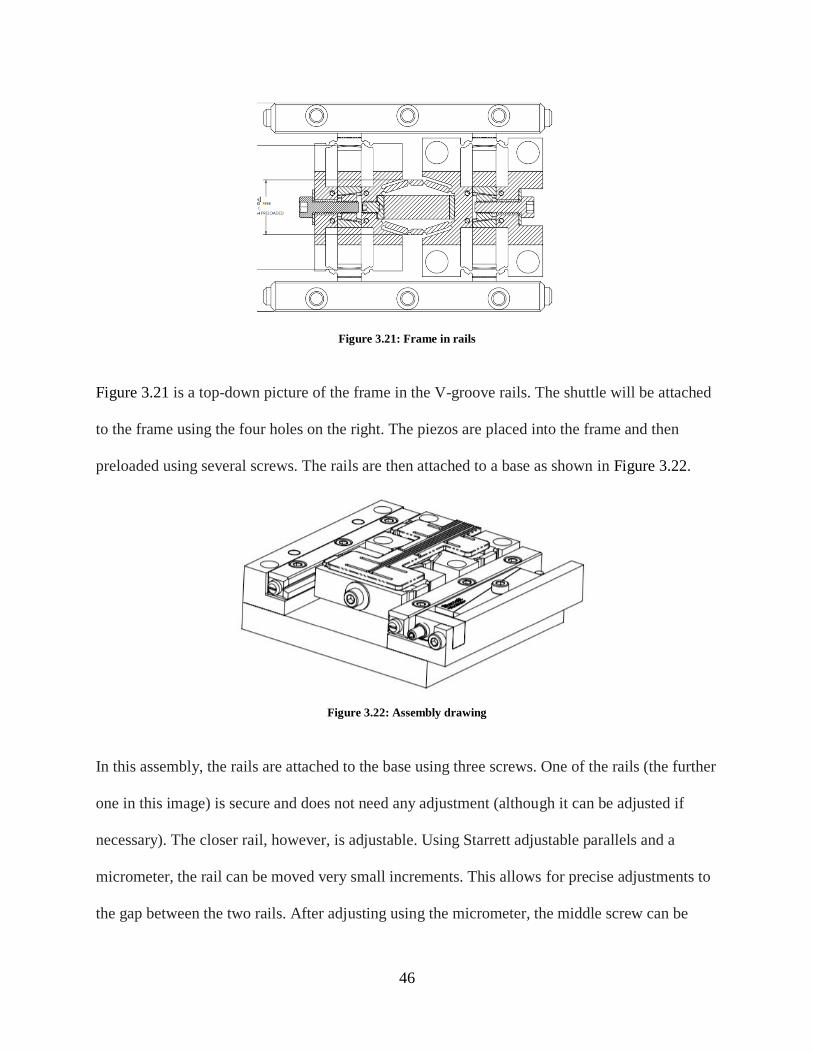
Figure 3.21 is a top-down picture of the frame in the V-groove rails. The shuttle will be attached
to the frame using the four holes on the right. The piezos are placed into the frame and then
preloaded using several screws. The rails are then attached to a base as shown in Figure 3.22.
In this assembly, the rails are attached to the base using three screws. One of the rails (the further
one in this image) is secure and does not need any adjustment (although it can be adjusted if
necessary). The closer rail, however, is adjustable. Using Starrett adjustable parallels and a
micrometer, the rail can be moved very small increments. This allows for precise adjustments to
the gap between the two rails. After adjusting using the micrometer, the middle screw can be
Figure 3.21: Frame in rails
Figure 3.22: Assembly drawing
Page 50
47
tightened first so that the entire rail pivots around that point. The outside screws can then be
tightened to achieve a desired angle.
3.4 Development of Z-axis
The Z-axis is a fast tool servo (FTS) that will move the tool during machining. The range
of this axis is small compared to the other axes and it will be moving at a high frequency in order
to create the desired geometry of the lens mold. Based on what was stated earlier, it will have to
oscillate its full amplitude (which needs to be greater than 35 µm) at 200 Hz. It will also need to
have a stiffness of 200 N/µm in the degrees of constraint. Lastly, the stresses experienced by the
mechanism need to be approximately half of the yield strength of the material that the axis is
made out of.
3.4.1 FTS Examples
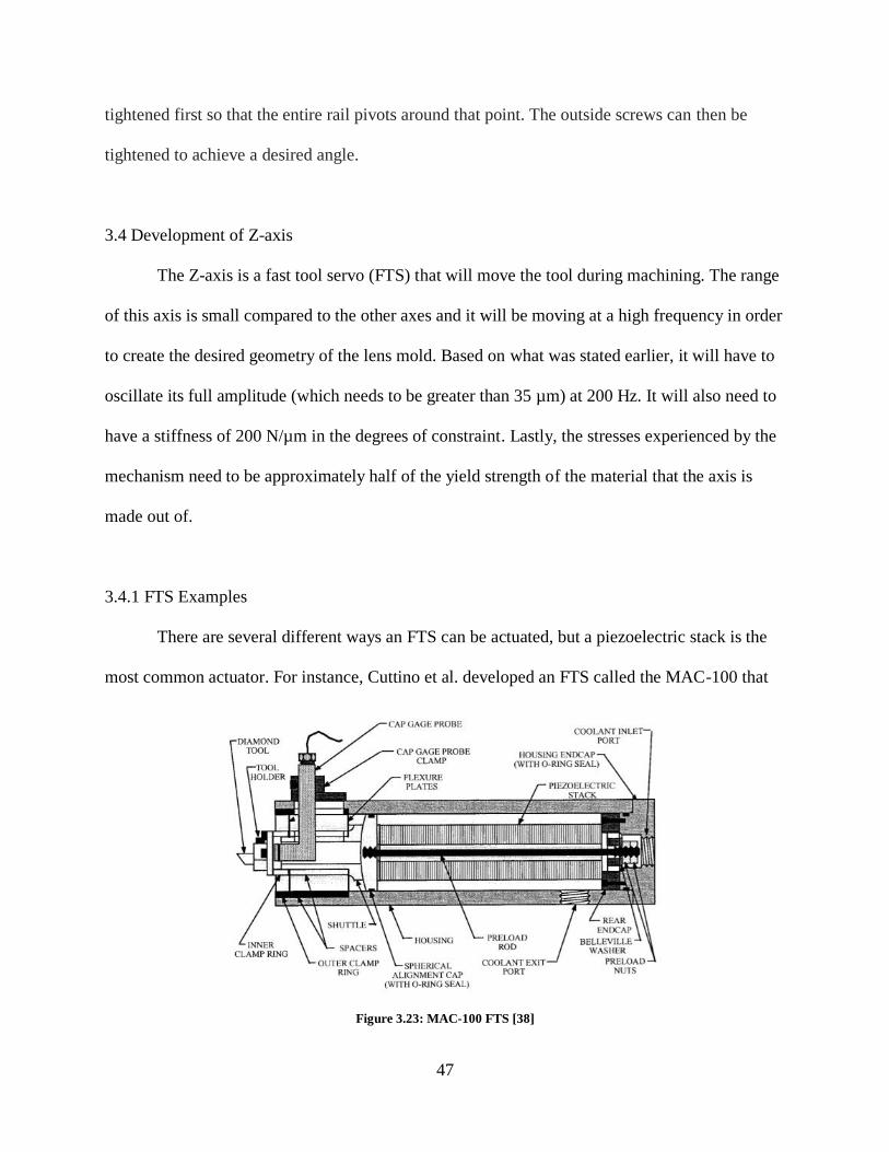
There are several different ways an FTS can be actuated, but a piezoelectric stack is the
most common actuator. For instance, Cuttino et al. developed an FTS called the MAC-100 that
Figure 3.23: MAC-100 FTS [38]
Page 51
48
used a very large piezo stack (13 cm) that had a range of 100 µm, a bandwidth of 100 Hz, a
resolution of 25 nm, and a stiffness of 70 N/µm in the direction of travel. Two flexure plates, a
preload rod, and a several preload nuts were used to provide the preload. These flexure plates
allow movement in the axial direction while providing adequate stiffness in the radial direction
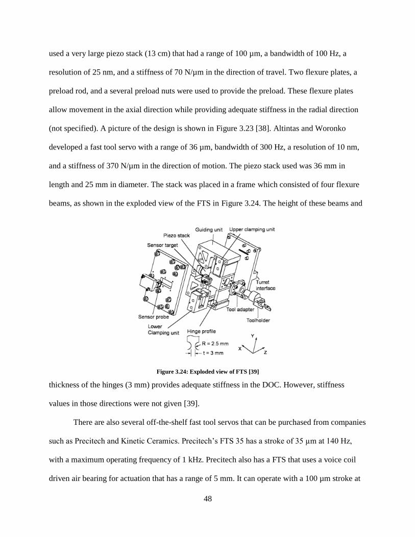
(not specified). A picture of the design is shown in Figure 3.23 [38]. Altintas and Woronko
developed a fast tool servo with a range of 36 µm, bandwidth of 300 Hz, a resolution of 10 nm,
and a stiffness of 370 N/µm in the direction of motion. The piezo stack used was 36 mm in
length and 25 mm in diameter. The stack was placed in a frame which consisted of four flexure
beams, as shown in the exploded view of the FTS in Figure 3.24. The height of these beams and
thickness of the hinges (3 mm) provides adequate stiffness in the DOC. However, stiffness
values in those directions were not given [39].
There are also several off-the-shelf fast tool servos that can be purchased from companies
such as Precitech and Kinetic Ceramics. Precitech’s FTS 35 has a stroke of 35 µm at 140 Hz,
with a maximum operating frequency of 1 kHz. Precitech also has a FTS that uses a voice coil
driven air bearing for actuation that has a range of 5 mm. It can operate with a 100 µm stroke at
Figure 3.24: Exploded view of FTS [39]
Page 52
49
440 Hz [40]. Kinetic ceramics has one FTS that operates at 20 kHz with a 10 µm stroke, one that
operates at 5 kHz with a 25 µm stroke, and one that operates at 100 Hz with a 400 µm stroke
[41]. Stiffness values were not provided for any of these devices and the price for any one of
these is too high for this research.
3.4.2 Initial Design
Like the above designs, a piezo will be used to actuate the Z-axis, as it has the capability
to actuate at high frequencies with high forces if paired with the correct electronics. The depth of
the lens is about 35 µm, so a piezo that can actuate at least that amount (preferably more) at a
minimum of 200 Hz (again, preferably more) is necessary. The selected piezo is 35 mm in
diameter, 61 mm long, has a nominal displacement of 60 µm, a stiffness of 430 N/µm, can
actuate at 400 Hz at its maximum displacement, and has a blocking force of 26 kN.
It seems that upon researching fast tool servo designs, a common design was the same
concept that was used when creating the X-axis. In short, a stage is suspended by flexures that
are attached on the other end to a wall, which is grounded. The actuator is then placed between a
wall and the stage. As it actuates, the flexures basically stretch to allow the stage to move.
Therefore, the further the stage moves, the harder it is to displace. While this design was
acceptable for the X-axis, it was deemed that since control of the FTS is much more difficult, it
would be better to design an axis that was linear in nature. In order to create a linear axis, it was
decided that a mechanism should be designed, specifically a straight line mechanism. There are a
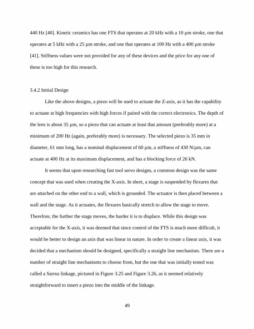
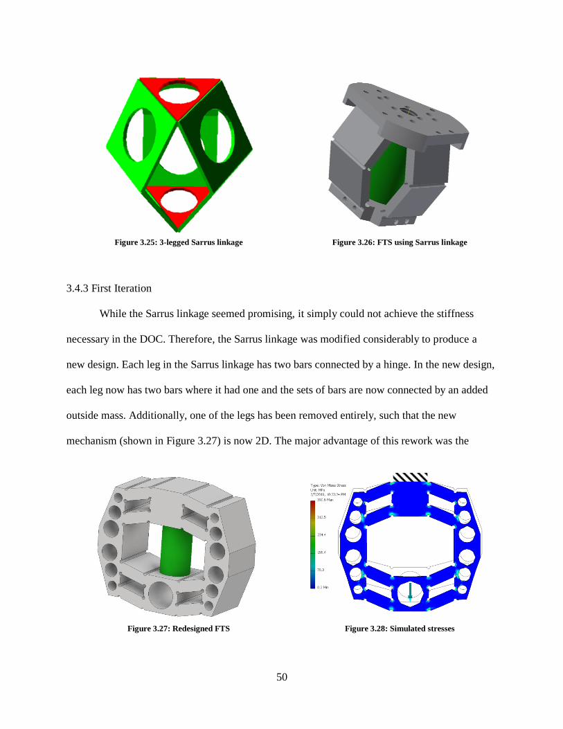
number of straight line mechanisms to choose from, but the one that was initially tested was
called a Sarrus linkage, pictured in Figure 3.25 and Figure 3.26, as it seemed relatively
straightforward to insert a piezo into the middle of the linkage.
Page 53
50
3.4.3 First Iteration
While the Sarrus linkage seemed promising, it simply could not achieve the stiffness
necessary in the DOC. Therefore, the Sarrus linkage was modified considerably to produce a
new design. Each leg in the Sarrus linkage has two bars connected by a hinge. In the new design,
each leg now has two bars where it had one and the sets of bars are now connected by an added
outside mass. Additionally, one of the legs has been removed entirely, such that the new
mechanism (shown in Figure 3.27) is now 2D. The major advantage of this rework was the
Figure 3.25: 3-legged Sarrus linkage
Figure 3.26: FTS using Sarrus linkage
Figure 3.27: Redesigned FTS
Figure 3.28: Simulated stresses
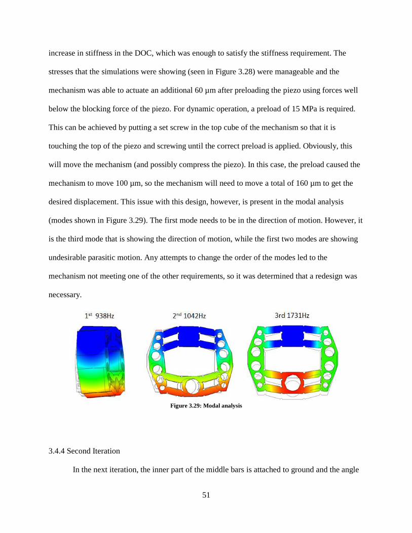
Page 54
51
increase in stiffness in the DOC, which was enough to satisfy the stiffness requirement. The
stresses that the simulations were showing (seen in Figure 3.28) were manageable and the
mechanism was able to actuate an additional 60 µm after preloading the piezo using forces well
below the blocking force of the piezo. For dynamic operation, a preload of 15 MPa is required.
This can be achieved by putting a set screw in the top cube of the mechanism so that it is
touching the top of the piezo and screwing until the correct preload is applied. Obviously, this
will move the mechanism (and possibly compress the piezo). In this case, the preload caused the
mechanism to move 100 µm, so the mechanism will need to move a total of 160 µm to get the
desired displacement. This issue with this design, however, is present in the modal analysis
(modes shown in Figure 3.29). The first mode needs to be in the direction of motion. However, it
is the third mode that is showing the direction of motion, while the first two modes are showing
undesirable parasitic motion. Any attempts to change the order of the modes led to the
mechanism not meeting one of the other requirements, so it was determined that a redesign was
necessary.
3.4.4 Second Iteration
In the next iteration, the inner part of the middle bars is attached to ground and the angle
Figure 3.29: Modal analysis
Page 55
52
of the bars is eliminated. The top and bottom portions were then attached by a beam and the
piezo was pulled outside of the mechanism, which is shown in Figure 3.30. Now that the tool tip
has a shorter path to ground, there is a significant increase in parasitic stiffness and the modal
analysis indicates that the first mode is indeed in the direction of motion. Looking at the parasitic
stiffness, one direction has a stiffness of 333 N/µm and the other a stiffness of 526 N/µm, which
exceeds the requirement of 200 N/µm. The mechanism moves 80 µm when preloaded with the
15 MPa necessary for dynamic operation and requires an additional 12.5 MPa from the piezo to
travel 60 µm further. This is about half of the piezo’s blocking force. The maximum stress seen
Figure 3.30: FTS - 2nd iteration
Figure 3.31: Modal analysis - 2nd iteration
Page 56
53
at maximum displacement is 300 MPa. There are several tool steels with a yield strength that is
twice that, so there should not be any problems with fatigue. As mentioned earlier, the first mode
in the modal analysis is in the direction of motion and occurs at a frequency greater than 800 Hz.
It is preferable to have the first mode occur at a minimum of twice the maximum operating
frequency.
3.4.5 Final Iteration
The issue with this design, however, is that the piezo is located outside the mechanism.
To make the design more compact, it would be desirable to place the piezo inside the
mechanism. Therefore, a final iteration was created that placed the piezo inside while keeping
the mechanism relatively the same. This design is shown in Figure 3.32. The top of the piezo is
now touching a beam that is rigidly attached to a plate that is grounded. This beam and plate are
separate from the mechanism and are used to provide a ground for the piezo and attach the FTS
to a manual slide so that the position of the axis can be adjusted. This design still satisfies all of
the requirements mentioned earlier. One concern that was only brought up after finishing this
design was that by preloading the piezo with this mechanism, a considerable amount of range
might be lost. Therefore, it was necessary to determine how much motion would be lost before
moving forward with this design.
Figure 3.32: FTS - final iteration
Page 57
54
3.4.6 Loss of Range Determination
Physik Instrumente details in their technical data on piezos how to determine this value
based on the type of preload that is applied. Since this mechanism is linear within a certain range
of motion (e.g. double the applied force leads to double the displacement), the axis can be treated
as a piezo with a spring preload. The plot in Figure 3.33 shows how to calculate the motion loss
based on nominal displacement, blocking force, and stiffness of the preload. ΔLo is the nominal
displacement, Fmax is the blocking force, and kL is related to the preload stiffness. kL is almost
completely defined by the hinge thickness of the flexure mechanism, so in order to increase the
slope of that line, the hinge thickness needs to be reduced. However, reducing the hinge
thickness also lowers the stiffness in both parasitic directions, so it is imperative that the parasitic
stiffness requirement is maintained while lowering the preload stiffness, thereby increasing the
slope of kL. PI recommends that the preload stiffness be an order of magnitude less than the
stiffness of the piezo, which is 430 N/µm. Therefore, the preload stiffness should be 43 N/µm. If
the hinge thickness is lowered such that the smaller of the two parasitic stiffnesses is exactly 200
N/µm, this can be achieved, but when looking at the modal analysis, the first mode now occurs at
Figure 3.33: Load case with spring preload
Page 58
55
500 Hz, which is too close to the operating frequency of 400 Hz. Therefore, it is necessary to
increase the hinge thickness until the first mode occurs at 800 Hz. When this was done, the
preload stiffness was 65 N/µm, which is pretty close to the goal. Moving forward, there are two
important lines: a line from the nominal displacement to the blocking force and a preload
stiffness line. The intersection of these two lines gives the actual displacement. For the piezo
with a 60 µm displacement and a 26 kN blocking force, the actual displacement ends up being 52
µm, which is greater than the 35 µm requirement. If a different piezo was used that had the same
displacement but a smaller blocking force, a smaller actual displacement would be observed. For
the piezo from PI with a 13 kN blocking force, the actual displacement would be 46 µm and for
the piezo with a 5.6 kN blocking force, the actual displacement would be 35 µm. Seeing these
results, it makes sense to stick with the original choice of piezo. With the current design, the
parasitic stiffness, range of motion, and maximum stress requirements are all met. The modal
analysis results are also satisfactory.
3.4.7 Amplifier Discussion
The last aspect to consider is using an amplifier in conjunction with the mechanism that
Figure 3.34: Intersections
Page 59
56
has been developed. This might allow the use of a piezo with a smaller displacement or increase
the displacement of the Z-axis that uses the piezo that was chosen earlier. If an amplifier is going
to be used, it will provide the preload, which means that the preload stiffness cannot be too high.
Unfortunately, if the preload stiffness is an order of magnitude lower than the piezo, the stresses
experienced when just adding the preload are unmanageable and will probably break the
amplifier before the preload can even be applied. Before talking about using an amplifier on the
already chosen piezo, it is important to lay out why it is not feasible to use a piezo with 30 µm
displacement in this axis. If there is a hypothetical amplifier that does not restrict the motion of
the piezo at all and a piezo with 30 µm displacement and a 23 kN blocking force is amplified by
three times, the displacement will be 90 µm and the new blocking force will be 23 kN (the
piezo’s blocking force) divided by three (7.67 kN). This line intersects with kL at 51 µm, which
is less than the 52 µm already obtained without an amplifier with the larger piezo. On top of that,
this is assuming no loss of motion from the amplifier itself, which is not possible. If a piezo with
a higher blocking force is selected and the calculations above are repeated, the actual
displacement is about 60 µm. However, with loss of motion from the amplifier, it is likely that
this number is also smaller than 52 µm.
If the already selected 60 µm displacement piezo is amplified, it might be possible to
improve the range of motion, but it leads to a lot of complications. The amplifier in Figure 3.35
Figure 3.35: Amplifier
Page 60
57
was designed in order to test whether or not it was worth amplifying the piezo chosen. There are
three ways that this amplifier can be designed. The first design is stiff and has low stresses. The
second has a stiffness that is an order of magnitude less than the piezo and has high stresses. The
third has a reasonable stiffness that is not an order of magnitude less than the piezo with fairly
high stresses. The problem with the first design is that it restricts the range of motion too much.
The problem with the second is that the stresses are unmanageable. The third design is
interesting because it restricts the motion of the piezo quite a bit and the stresses are much higher
than the stresses seen in the mechanism, but it does seem like it is possible to get a little more
motion. In one simulation, the range of motion came out to be 61 µm, which is an improvement
over the 52 µm value seen before, but the forces required by the piezo in this design and the
stresses experienced make it likely not worth using over the design without an amplifier. From
these calculations and simulations, it seems that it does not make sense to use an amplifier with
this axis.
3.5 Summary
In this chapter, three axes for an ultraprecision machine were individually developed to
meet a number of requirements that were laid out in the first section. These requirements
included stiffness, resolution, maximum stress, and range. The simulations to determine if an
axis met these requirements were all done using Autodesk Inventor and Autodesk CFD. The X-
axis, a single degree of freedom flexure axis actuated by a voice coil, was designed such that it
could travel at least the width of one lens, would have the ability to follow a low frequency sine
wave command, would have the capability to have high resolution, was very stiff in the degrees
of constraint, had manageable stresses, and would not heat up to temperatures that would cause
Page 61
58
the beams to expand. The Y-axis, an inchworm axis driven by five piezos, was designed to have
a much larger range. It also met the resolution, stiffness, and stress requirements, but was
designed to step to a position and lock in place, as opposed to following a waveform. Both the X-
and Y-axes were manufactured for testing, while the Z-axis was not. The Z-axis, a fast tool servo
driven by a large piezo, was designed such that it had the range of the depth of one lens. It also
met the resolution, stiffness, and stress requirements, but was designed to follow very high
frequency waveforms. The Z-axis is theoretically capable of actuating its full range at 400 Hz.
Page 62
59
Chapter 4: Testing and Results
This chapter will discuss the testing of the manufactured X- and Y-axes. It will be broken
into two sections. One section will cover the testing of the X-axis, which includes testing the
stiffness and amount of parasitic motion while actuating. The other section will cover the testing
of the Y-axis, which includes testing the stiffness, speed, and closed loop resolution. A few other
tests will also be performed to determine if the stiffness can be increased or if the jerking can be
reduced or eliminated. This section will also cover how the closed loop was implemented for the
Y-axis.
4.1 X-axis Testing and Results
After some very slight modifications to the beam clamps from the design seen in Chapter
3, the axis was manufactured in order to begin testing. The axis is shown in Figure 4.1. All parts
were made out of aluminum (except for the beams and Macor plates) to reduce the cost and ease
the process of manufacturing. A torque wrench was used to tighten all of the beams to around the
Figure 4.1: Manufactured X-axis
Page 63
60
same tension. Initial testing was performed by commanding the voice coil using a DSpace
controller board, which sent signals to a Galil amplifier. A capacitance gauge was used for
feedback, but unfortunately, the capacitance gauge only has 160 µm of range, which is not
enough to measure the full range of the axis. Capacitance gauges are non-contact, high resolution
measuring devices that measure the capacitance between the sensor and a conducting object to
determine the distance between the sensor and the object [42]. By attaching the gauge to a
micrometer stage, it was possible to approximate the range of the stage as 3 mm by applying
voltage to the voice coil, noting the distance traveled, moving the capacitance gauge back into
range using the micrometer stage, and then repeating the process.
4.1.1 Stiffness Testing
After finding the range, tests were performed to find the stiffness in the two parasitic
directions (the y- and z-directions, in this case). To do this, a weight was placed so that the force
was acting in one of the parasitic directions and a capacitance gauge was set up to read the
movement. The two setups are shown in Figure 4.2. The initial test showed a stiffness of 25
N/µm in the z-direction, which seemed very low compared to the simulated value. Using the
Figure 4.2: Stiffness setups
Page 64
61
clamps to tension the beams, the stiffness was again measured and the result was 60 N/µm in
both parasitic directions. Since the beams were tightened, it is safe to assume that some range of
motion was lost. After tightening, the range when inputting a 4 V amplitude sine wave was only
1 mm. A fiber optic displacement sensor, which is another non-contact measuring device, was
used to take this measurement, which has more range than a capacitance gauge (3 mm vs. 160
µm), but a worse resolution (300 nm vs. 2.5 nm). This sensor works by transmitting a beam of
light, receiving the reflected light from the target surface, and then converting this light into an
electrical signal that corresponds to the distance between the sensor and the target [43].
Unfortunately, the power supply used with this axis would shut off if the amplitude was any
higher, so the full range of the axis could not be determined. 60 N/µm is a high stiffness, but,
again, not as high as what the simulations showed. However, when stiffness tests on the
inchworm axis were performed (details will be discussed later), it was found that proper
clamping was absolutely necessary to get a proper stiffness reading, which was not done when
testing the stiffness of the X-axis. Therefore, it is likely that the stiffness of the X-axis is actually
higher than the 60 N/µm result received.
4.1.2 Parasitic Motion Testing
After testing the stiffness, tests were performed to determine the parasitic motion of the
axis when actuated. As in, measure how much it moves in the y- and z-directions when actuating
the voice coil. To do this for the y-direction, a silicon wafer (because of its flatness) was
mounted on top of the stage and a capacitance gauge was set up to read the movement of the
wafer in the y-direction. For the z-direction, a capacitance gauge was placed so that is was
measuring the actual stage. A graph of the result for the y-direction is shown in Figure 4.3. It is
Page 65
62
apparent that there are three distinct regions in this graph: when the voice coil is pushing
outwards (Region 3), when the voice coil is pulling inwards (Region 1), and the middle (Region
2). There are several takeaways from this graph. To start, it is apparent that the region where the
voice coil is pushing has less noise than when the voice coil is pulling, but the two regions have
the same consistent slope. This indicates that the axis has relatively little parasitic motion in the
y-direction and the only reason for the slope is because of the angle of the mounted wafer.
However, a change in slope is noticeable when the axis is moving through the middle region.
Region 2 contains a singularity where the axis has essentially no stiffness in the direction of
motion, so this could be the explanation for this odd behavior. The stage could be translating in
the y-direction or twisting to cause this change in slope. Another possible explanation is that it is
related to the electronics being used when switching between a positive and negative voltage.
When looking at the z-direction motion, shown in Figure 4.4, the result is very similar.
The same three regions appear, with the only noticeable difference being that the slope of the
Figure 4.3: Y-direction parasitic motion
Region 1 Region 2 Region 3
Page 66
63
push and pull regions is essentially zero, which is good, as the stage is being measured directly.
Something to note is that when the power supply was turned off, the width of the reading
dramatically decreased. When the voice coil was actuated using a variable power supply, the
width of the reading while the axis was moving was still reduced. What was most interesting,
however, was that the width of the reading was almost the same on both sides of the singularity.
When applying a negative voltage, the width went from 1.2 µm to 0.2 µm and when applying a
positive voltage, the width went from 0.32 µm to 0.16 µm. It is safe to assume, then, that the
electronics are greatly affecting the performance of the X-axis and new ones will need to be
purchased in order to properly run this axis.
4.2 Y-axis Testing and Results
There are more pieces that will be added to this axis to increase stability and rigidity,
allow for easier attachment to the x-axis, and allow for easier encoder placement, but for now,
Figure 4.4: Z-direction parasitic motion
Region 1 Region 2 Region 3
Page 67
64
the prototype in Figure 4.5 has been manufactured. The wires from the piezos have been routed
through a small plastic piece that sits on top of the frame. This is most likely a temporary
solution. These wires will be connected to an amplifier, specifically a three-port Cedrat amplifier
with a gain of 20 that allows for the piezos to be driven at a maximum frequency of about 130
Hz. Although five piezos need to be driven, only three channels on the amplifier need to be
utilized, as the two piezos that make up one clamp receive the same signal. Initially, the
amplifier was simply connected to an Arduino that produced square waveforms as shown in the
picture of an oscilloscope screen in Figure 4.6. The yellow waveform is the waveform used to
control the extension piezo. The blue and green waveforms are identical, but have a phase offset.
There is a continuous line made from the green and blue signals, indicating that at least one
Figure 4.5: Inchworm assembly
Figure 4.6: Generated waveforms
Page 68
65
clamp is always engaged during movement. With this setup and a voltage divider (since it is
recommended that the extension piezo not be operated continuously at 100 V), open loop testing
could begin.
4.2.1 Axis Movement
The first task was simply to get the axis running. In order to do that, the piezos were
hooked up to the amplifier, a small amount of code was written to command the Arduino, and a
camera with a macro lens was used to observe the movement. Without much rail adjustment, the
axis started moving. Once a ruler was placed next to the frame, it was easier to see the
movement. The video footage gathered from the camera was input into a program called tracker
in order to look at the motion. Afterwards, a capacitance gauge was set up to measure the
movement of the frame. This setup is shown in Figure 4.8. The capacitance gauge is held using
optical components and a magnet that is attached to the pneumatic table. The base of the
inchworm axis is lightly clamped down on one side. This capacitance gauge is connected to
DSpace, which is a controller board with several ADCs and DACs. The voltage produced by the
capacitance gauge can be read using the associated DSpace software. The voltage ranges from -
10 to 10 V, with each volt representing about 8 µm of movement, meaning that the range is only
Figure 4.7: Zoomed in view of frame
Page 69
66
160 µm. Theoretically, the resolution of the capacitance gauge is supposed to be 2.5 nm, but
even with proper grounding, the best resolution achieved was only 25 nm. This is most likely due
to vibrations that cannot be accounted for and some electrical noise. Below in Figure 4.9 are two
graphs that show the first measurement gathered using the capacitance gauge. The graphs show
that the axis traveled about 12 µm (1 volt ≈ 8 µm) back and forth several times. Something else
to note is that there is a drift occurring, as in, the axis is not returning to the spot it started from.
If the graph is zoomed in, the individual steps of the process can be seen. As stated before, there
are six steps that occur. Figure 4.10 labels when these steps are occurring. It is evident that there
is movement in the direction of motion when the clamps are expanding and contracting.
Obviously, this is not desired, as the frame should stay in place except for when the extension
Figure 4.8: Capacitance gauge setup to measure displacement
Figure 4.9: Displacement graphs
Page 70
67
piezo is moving.
4.2.2 Stiffness Testing
After seeing this movement, the next tests performed on the axis were stiffness tests. The
first direction tested was in the direction of motion, since the capacitance gauge was already set
up to read that direction. The base of the axis was clamped down and a weight was tied to one
end of the frame. This weight was hung over the edge of the table using a pulley. Since this axis
will not be moving while machining is occurring, both clamps should be engaged for this test
Figure 4.10: Zoomed in displacement graphs
Figure 4.11: Setup for testing stiffness in direction of motion
Page 71
68
and all future stiffness tests. By sending 100 V to each of the four piezos that make up the
clamps, the axis can effectively be locked into place and then the stiffness can be tested. The
setup for this test is shown in Figure 4.11. Once both clamps were engaged, the 0.5 kg weight
was slowly dropped off the side of the table and the movement of the frame was recorded by the
capacitance gauge. The weight was then lifted. The measured stiffness was 125 N/µm, which is
lower than the 200 N/µm requirement, but is still an incredibly high stiffness. When the weight
was lifted, the reading returned to where it was before the force was applied, which means that
the frame is not sliding within the guides. Something else is moving, whether that means that it is
the rails, the base, or a part of the frame. Afterwards, the brake was removed and it was made
sure that the axis could still move as intended. Not only did it move as before, but it was actually
moveable by hand. This was important to check to make sure that the large stiffness value
observed was not due to the gap between the rails being too small. If everything is functioning
properly and a stiffness that high can be achieved when the brake is applied, this axis should
perform well during machining.
The next step is to test the stiffness in the other two directions. One direction is
downwards (vertical stiffness) and the other is in the direction of machining (lateral stiffness).
The setups to test these stiffnesses are shown in Figure 4.12, but these were not the original
Figure 4.12: Setup for testing stiffnesses (lateral, vertical)
Page 72
69
setups. When the stiffnesses in these directions were first tested, the results were less than stellar.
Stiffnesses of 20-30 N/µm were observed in both directions, which does not meet the
requirements set earlier. However, it was eventually realized that the entire base was moving
when the tests were being performed, indicating that the base was not properly clamped to the
table. To confirm this, the stiffness tests were performed again, but instead of measuring the
movement of the frame, the movement of the base was measured. After this realization, the base
was clamped down using a different method and the stiffnesses were measured again. Starting
with the lateral stiffness (x-direction), two methods were used to determine the stiffness. The
first method was similar to the method discussed earlier. A weight was attached to the frame and
hung over the side of the table. For the second method, a load cell was used to push on the frame
to determine how much force was being applied. Also, it was decided that even though the base
was clamped better than before, the movement of the frame and the movement of the base should
be measured and the difference should be taken to determine the stiffness. Figure 4.13 illustrates
where the
force was applied and where measurements were taken. The tests resulted in a stiffness anywhere
between 70 and 100 N/µm. Figure 4.14 shows the movement of the frame (blue) and base (pink)
in microns. When the force is removed, the frame more or less returns to its original position.
Figure 4.13: Placement of force and gauges (lateral)
Page 73
70
Moving onto vertical stiffness, a similar procedure was used. Figure 4.15 shows where
the load was applied and where measurements were taken. Figure 4.16 again shows the
movement of the frame (blue) and base (pink). The stiffness in this direction was very similar,
between 60 and 100 N/µm. The stiffness in this direction is high, same as the lateral direction.
Figure 4.14: Lateral stiffness graph
Figure 4.15: Placement of force and gauges (vertical)
Figure 4.16: Lateral stiffness graph
Page 74
71
However, it was not possible to place the load directly where the machining would take place, so
some of the movement seen could be due to rotation. Also, in the final design of this axis, there
are cross roller bearings below the frame. This might improve the stiffness, but until the design
incorporates them, the effect they will have on the stiffness will be unknown.
4.2.3 Increasing Stiffness
To perform the next few tests, control of the axis was moved over to the DSpace
controller mentioned earlier. This allows for much more control over the signals that are being
sent to the piezos. Before, the magnitude and shape could not be easily altered. Now, these
parameters can be changed as the axis is running and switching between the three modes
(forward, reverse, and brake) can be done quickly. This is still all in open loop, but the eventual
goal is to move to a closed loop controlled by a Delta Tau PMAC controller using Renishaw
linear encoders for feedback. This also applies to the X-axis.
Now that more precise control over the piezos was possible, a few tests were run in an
attempt to increase stiffness. One of these tests involved adjusting the rails to see the effect of
moving them closer to one another. The movement was measured using a capacitance gauge and
the movement was plotted. Each time the axis was able to successfully move, the micrometer
was adjusted by a small, fixed amount and the axis was run again. This was done until the axis
Figure 4.17: Simulink program and DSpace graphing software
Page 75
72
hardly moved. Every time the gap between the rails became smaller, the slope of the
displacement vs. time graph decreased. It was assumed that this was due to the extension piezo
having to overcome more friction. Figure 4.18 shows the slopes of two of the tests (first and
last). The stiffnesses were then retested to determine if the stiffness in any direction changed.
Based on the tests, it was determined that changing the rail distance does not change the
stiffness. The next test performed attempts to determine if increasing the voltage applied to the
clamps increases the stiffness at all. Again, it was found that the stiffness values were no
different when the voltage applied was 100 V or 150 V.
4.2.4 Open Loop Resolution Test
The next test run was a resolution test. To do this, the voltage of the extension piezo was
lowered further and further and the step size was observed each time. The lowest step size seen
was 100 nm, but this was the lowest step size achieved. When 0 V was applied to the extension
piezo (only the clamps were moving), the step size was still 100 nm, which is shown in Figure
4.19. This means that even when a voltage is not being applied to the extension piezo, the clamps
are moving the axis. This is due to the positioning of the rails. By changing the positioning of the
rails, it was possible to actually reverse the direction of this observed bias, which means it is
Figure 4.18: Rail tightening tests
Page 76
73
certainly possible to reduce the bias by trial and error. In a future design, it might be worth
adding micrometers to the two ends of the adjustable rail so the angle of the rail can be more
precisely adjusted.
4.2.5 Closed Loop Testing
The next step was to move to closed loop testing. Originally, the PMAC was going to
control the inchworm, but instead it was decided that the PMAC should send a voltage to a
microcontroller (Arduino in this case) based on the feedback that the PMAC was receiving. The
Arduino would then take this voltage and based on its value, tell the inchworm to either move
forward, move backward, or brake. The PMAC sends a voltage from a 16-bit DAC based on the
following error (2.5 V is zero following error) and the gains set in the software. The Arduino
receives this signal using a 10-bit ADC and if the signal is greater than 2.5 V and the absolute
value of the signal minus 2.5 V is greater than the deadband set, then the Arduino will command
a forward step. If the signal is less than 2.5 V and the absolute value of the signal minus 2.5 V is
greater than the deadband set, then the Arduino will command a backward step. Otherwise, the
Arduino commands the inchworm to stay in place by expanding both clamps. In the first setup,
the command to the extension piezo was sent using a 12-bit DAC and the clamp piezos were
Figure 4.19: Clamps only steps
Page 77
74
controlled with a digital signal.
For this axis, the only thing that matters is that this inchworm is able to perform accurate
steps, as this axis simply moves to a commanded position and brakes. Therefore, the only tests
that will be performed are step responses. The piezos are run at 50 Hz while performing these
steps, because at any frequency higher than that, the amplifier attenuated the signal. Only
proportional gain was used in the initial tests. A graph of a 1 µm step is shown in Figure 4.20. It
took 12 individual steps to get to the commanded position and took a little longer than 0.2
seconds, which lines up with the 50 Hz operating frequency. In this particular test, the axis
stopped almost exactly on the commanded position, but this was not always the case. The error is
more obvious when looking at a 100 nm step, like the one shown in Figure 4.21. In order to get
rid of this error, an integral gain needs to be added, but even when one was added, unacceptable
errors were still occurring. This was due to the fact that the ADC was only 10-bits. Since the
resolution of the ADC was so poor, it would not recognize that it was receiving different signals
from the PMAC’s DAC. The PMAC would then attempt to apply more and more control effort
Figure 4.20: 1 µm step without integral
Page 78
75
because the error was not reducing and when the Arduino finally recognized a change, it would
apply too much of a correction due to the buildup of the integral.
Several steps were taken in order to improve the step response of the inchworm. A 16-bit
ADC IC was purchased to use with the Arduino and a much better deadband was obtained due to
this upgrade. The deadband is a range around the commanded position where control effort is
shut off if the axis is within that range. However, the PMAC control algorithm does not shut off
integral control when the axis is within the deadband for some reason, so a PLC (programmable
logic controller) was created to turn off integral control if the axis is within the deadband for a
certain amount of cycles. Additionally, the sequence of one step was changed from the order
presented in Figure 3.13 earlier. Instead of the last step having one of the clamps contracted, it
was changed so that the last step of the process had both clamps expanded. The issue before was
that if the system determined the axis was in deadband, one of the clamp piezos would expand
and the axis would move. This way, when the control loop finishes and returns to the top of the
loop, if the system determines the axis is in deadband, no piezos will have to move to put it in the
Figure 4.21: 100 nm step without integral
Page 79
76
brake position. Lastly, the Arduino and PMAC were synced by sending a digital signal from the
Arduino to the PMAC when the inchworm completes a step. Before, the PMAC was taking
readings at all points during the inchworm’s movement, but the only data point that matters is
when the inchworm has completed a step and is stopped. Therefore, it was made such that the
PMAC only updates the position of the axis when it receives a signal from the Arduino. This also
makes the step test graphs look cleaner.
With all of these changes, the step response of the axis was retested starting with 1 µm
steps. A series of them and a single step from that series is shown in Figure 4.22. The steps took
about 0.5 seconds to complete and the error was ±5 nm. There was a significant overshoot in
some of these steps, so proportional gain might need to be toned down. A 100 nm step is shown
in Figure 4.23. This step only took a tenth of a second to complete and still had a considerable
overshoot. Finally, 10 nm steps were taken and are shown in Figure 4.24. The noise of the
capacitive gauge is about 10 nm, which is easy to see in the 10 nm step graph. Steps less than 10
nm have not been tested, but when the 1 nm resolution encoders are made available, more step
tests might be performed. Therefore, at this point, it is accurate to say that the closed loop
resolution of the inchworm axis is 10 nm.
Figure 4.22: 1 µm step with changes
Page 80
77
4.2.6 Jerking
The last tests attempted to improve the axis were to eliminate or reduce the jerking seen
when the axis is moving. Jerking is movement of the entire axis when one of the clamp piezos is
Figure 4.23: 100 nm step with changes
Figure 4.24: 10 nm steps
Page 81
78
expanding or contracting. Ideally, the axis would only move when the extension piezo moves,
but that is not what is happening. Significant movement is observed every time one of the clamps
moves. Initially, it was thought that this might be happening because the clamps are slamming
into the walls at high speeds and forces due to them being controlled digitally. A DAC was
purchased in order to test the theory that controlling the clamps with a DAC instead of a digital
signal might reduce this effect. Instead of quickly switching between 0 V and 100 V, a ramp
Figure 4.25: Generated control signals, trapezoid
Figure 4.26: Square vs. trapezoid jerking comparison
Page 82
79
between 0 V and 100 V was commanded, as shown in Figure 4.25. Figure 4.26 shows the graphs
when using trapezoid signals and square signals to control the clamps and it is apparent that there
is no difference in the magnitude of the large dips present. The next test reduced how much the
clamps expanded to see if that would make a difference, but there was no noticeable change.
Since none of these measures taken reduced the jerking, it was determined that the expansion and
contraction of the clamps is causing some significant and unwanted frame bending.
4.3 Summary
In this chapter, several tests were performed on the X- and Y-axes to determine how well
they will perform if used in an ultraprecision machine. For the X-axis, it was found that in the
degrees of constraint, the stiffnesses were both 60 N/µm, which does not meet the stiffness
requirement of 200 N/µm, but it is very possible that the actual stiffness value is much higher,
due to poor clamping of the X-axis. It was also found that there was almost no parasitic motion
when the axis was being actuated, except for a large jump when the axis crossed the zero point.
While the jump could be mechanical, it is more likely that the electronics are causing this issue.
The electronics also made it difficult to determine the full range of the axis and put the axis in a
closed loop. For the Y-axis, it was found that the stiffness in the direction of motion was 125
N/µm (again, it is possible that this number is higher) and the stiffnesses in the degrees of
constraint were between 60 N/µm and 100 N/µm. This does not meet the 200 N/µm requirement,
but the stiffness in all directions is still quite high. The stiffness could not be increased by
changing the distance between the rails or increasing the clamp voltage. There is a drift that is
determined by the angle of the rails, so the rails will need to be properly aligned to reduce this
drift as much as possible. When put into closed loop, the axis was capable of 10 nm steps using
Page 83
80
only proportional and integral control. The speed of the axis is 150 µm/s, but it is possible to
increase this speed by using different amplifiers. There was an attempt to reduce jerking, but
none of the methods proved successful, meaning that the frame would most likely need to be
modified in order to reduce jerking. However, this should not negatively affect the performance
of the Y-axis during machining. Further tests need to be done with 1 nm resolution Renishaw
absolute linear encoders to check the current findings.
Page 84
81
Chapter 5: Conclusions and Future Work
5.1 Conclusions
In this thesis, the development of three axes to be used in an ultraprecision shaping
machine was presented. All three of these axes were designed such that the cost of the
components and manufacturing would be significantly less expensive than purchasing an off-the-
shelf product to perform the same function. They were also designed to meet several
specifications determined necessary for the proper machining of a microlens mold in Stavax.
Each axis had to meet specific stiffness, range of motion, resolution, and stress requirements.
Two of these axes were manufactured for testing to determine if they were suitable for
ultraprecision machining. The following two subsections discuss the conclusions from the
development of the three axes and the testing of the two axes.
5.1.1 Axis Development
1. After ruling out the possibility of using a two degree of freedom stage for this research,
due to it not meeting the stiffness requirements, it was decided that the X-axis would be a
flexure-based, single degree of freedom axis. This axis is non-linear, as it requires more
force to move a specific distance when away from the zero point than when at the zero
point. The final design consists of three spring steel beams that are strung across from
one grounded wall to another. These beams are attached to the stage that will hold the Y-
axis and the voice coil that actuates this axis. Simulations on this design showed that the
stiffness in the parasitic directions would be 200 N/µm, range of motion would be 5 mm
(based on the force provided by the voice coil), and stresses would not exceed half the
yield strength of the spring steel beams, meaning that the axis should not fail due to
Page 85
82
fatigue. Heat transfer simulations were performed and based on the results, Macor
ceramic was added in between several components to help reduce heat flow from the
voice coil to the beams. A cooling system using water was also designed so that the
simulations showed no temperature increase in the beams. This cooling system has not
yet been implemented.
2. The Y-axis needed to have significantly more range than the X-axis, but since it was
determined that the Y-axis simply needed to act as a stepper axis and the speed of the
axis did not matter, it was decided that the Y-axis would be an inchworm axis, since the
range of an inchworm axis is effectively unlimited. An inchworm axis has clamps and
extenders that allow for movement if they are activated in a particular sequence. In the
final design, each of the two clamps is made up of two piezos and the one extender is
simply a single piezo. Using a piezo for the extender will allow for a high resolution axis.
The only way to assemble these piezos is to place them in a frame, which also provides
the preload for each piezo. The frame is asymmetrical so that a shuttle can be securely
attached to the top of the frame. The reason that each clamp consists of two piezos is so
that there can be a bar in between them. If machining occurs over this bar, stiffness
dramatically increases than if machining occurs over the middle of the frame, according
to the simulations.
Simulations were performed on the frame until the stiffnesses in the x- and z-
directions were greater than 200 N/µm, it was determined that the piezos would be able
to actuate within the frame, and the stresses were less than half the yield strength of the
steel being used to create the frame. The stiffness in the direction of travel is dependent
on the force output of the clamp piezos and the angle of the rails that the clamps extend
Page 86
83
into. These rails are attached to a base that will be mounted on to the top of the X-axis
stage. One of the rails is adjustable so that the distance and angle between the rails can be
changed when appropriate.
3. Based on some frequency decomposition calculations, it was determined that the Z-axis
would need to actuate the depth of one lens at a frequency of 200 Hz. Therefore, it was
decided that the Z-axis would need to be a fast tool servo, which is an axis with high
acceleration capabilities. The final design uses a piezo with 60 µm of range that can run
at 400 Hz. This piezo is placed in a steel frame that provides the preload and also makes
the axis stiff in the degrees of constraint. The frame is a mechanism that uses flexure
hinges. Because the frame is a mechanism and therefore linear, the axis will be easier to
control when in closed loop. Simulations were performed on the frame until the
stiffnesses in the x- and y-directions were greater than 200 N/µm, the stiffness in the
actuation direction was about an order of magnitude less than the stiffness of the piezo
(recommended by the company the piezo will be purchased from), and the stresses were
less than half the yield strength of some common tool steels. Based on the stiffness in the
actuation direction, some motion will be lost. It was determined that with this frame, the
axis would have a range of 52 µm, which is acceptable. Modal analysis simulations were
also performed to ensure that the first mode was in the direction of motion and that it
occurred at a frequency at least twice the maximum operating frequency.
5.1.2 Performance Testing
Tests were performed to find the axes’ stiffnesses, ranges, and resolutions, among other
characteristics. For the X-axis, the determined stiffnesses in the degrees of constraint were 60
Page 87
84
N/µm, although, new information suggests these numbers might actually be higher. The range is
at least 1 mm, but the full range cannot be determined until new electronics are purchased to
drive the voice coil. The resolution has yet to be determined, but given that it is a voice coil
pushing a flexure system, it is safe to say the resolution will be less than the 10 nm requirement.
There is also movement in the parasitic directions when the axis crosses its singularity and the
reasoning for this is still unknown. It seems, however, highly unlikely that it is mechanical. Most
likely, it is an issue with the electronics. For the Y-axis, the determined stiffness in the direction
of motion was 125 N/µm and the stiffnesses in the degrees of constraint were between 60 and
100 N/µm. Moving the rails closer together did not seem to have an effect on stiffness.
Increasing the voltage of the clamp piezos also did not seem to have an effect on stiffness.
The range of the axis is only limited by the length of the rail and the range of the
feedback device. The closed loop resolution is at least 10 nm, shown by the 10 nm step tests
performed. The speed of the axis is 150 µm/s, which should be acceptable. However, this speed
could be increased if different amplifiers were purchased to run the piezos at a higher frequency.
The maximum frequency that the piezos can currently run at is 50 Hz.
In an attempt to reduce jerking (unwanted movement of the entire axis when the clamps
are actuated), the waveform used to command the piezos was changed from a square wave to a
ramp. This change did not reduce jerking at all. Reducing the distance the clamps needed to
travel before contacting the rails also did not reduce jerking. All the tests for the X- and Y-axes
were performed with a capacitance gauge or a fiber optic displacement sensor, but eventually, an
optical linear encoder with 1 nm resolution will be used for feedback instead.
Page 88
85
5.2 Future Work
Below is a model of what the final machine will likely look like. The X-axis (single
degree of freedom flexure axis) is on the bottom, the Y-axis (inchworm axis) is attached to the
X-axis, and the Z-axis (fast tool servo) is attached to a manual slide that sits above the other two
axes. These components will be attached to a granite block.
The list below presents the future work that needs to be done in order to complete this research.
1.) Closed loop testing for the X- and Y-axes with the Renishaw encoders will need to be
performed to assess characteristics such as repeatability and accuracy.
2.) Machining tests with a diamond tool should be performed on aluminum using the two
axes already manufactured. The diamond tool will be attached to a servo (not the one
designed in this thesis) and the Y-axis will be attached to the top of the X-axis as
presented earlier. The goal would simply be to face a small piece of aluminum so that it
has a mirror finish.
Figure 5.1: Final machine model
Page 89
86
3.) Machining tests should be performed on Stavax using a CBN tool. The low stiffness of
the servo mentioned above might make it difficult to achieve a mirror finish.
4.) The fast tool servo design needs to be finalized and the axis needs to be manufactured. It
is likely that this axis will heat up quite a bit during operation, so a cooling system for the
FTS needs to be designed. Once the axis has been manufactured, testing, both open and
closed loop, will start immediately. Closed llop and open loopTesting should be
conducted
5.) The granite block/gantry, pneumatic isolators, and manual Z-slide need to be purchased
once all three axes have been manufactured.
6.) The axes need to be individually tested at their maximum performance in order to
determine exactly what type of cooling system will be needed for the machine.
7.) Once the entire system has been assembled, a motion program will need to be written to
control all three axes at once. Initially, simple motion programs should be written and
once those are working well, work can be started on the motion program that will be used
to machine the aspheric microlens array.
8.) Once that is complete, machining of the actual array can be attempted. The profile of the
array will then need to be measured and based on the results, certain aspects of the
system will need to be tweaked until the desired aspheric microlens mold is created.
Page 90
87
References
[1] Y. Shaohui, J. Hongpeng, Z. Guanhua, C. Fengjun and Z. Kejun, "Review of small asperic
glass lens molding technologies," Frontiers of Mechanical Engineering, pp. 66-76, 2017.
[2] "Smartphone production volume worldwide from 2015 to 2018 (in million units)," statista,
2018. [Online]. Available: https://www.statista.com/statistics/742517/global-smartphone-
production-volume/. [Accessed 18 June 2018].
[3] W. Yuan, L.-H. Li, W.-B. Lee and C.-Y. Chan, "Fabrication of Microlens Array and Its
Application: A Review," Chinese Journal of Mechanical Engineering, 2018.
[4] T.-H. Lin, H. Yang and C.-K. Chao, "Concave Microlens Array Mold Fabrication in
Photoresist using UV Proximity Printing," in DTIP, Stresa, 2006.
[5] J. Albero, L. Nieradko, C. Gorecki, H. Ottevaere, V. Gomez, H. Thienpont, J. Pietarinen, B.
Päivänranta and N. Passilly, "Fabrication of spherical microlenses by a combination of
isotropic wet etching of silicon and molding techniques," Optics Express, vol. 17, no. 8,
2009.
[6] L. Hui, L. Likai, N. N. J., R. J. W. and Y. A. Y., "Micro-optical fabrication by ultraprecision
diamond machining and precision molding," Frontiers of Mechanical Engineering, pp. 181-
192, 2017.
[7] P. Gao, Z. Liang, X. Wang, T. Zhou, J. Xie, S. Li and W. Shen, "Fabrication of a Micro-
Lens Array Mold by Micro Ball End-Milling and Its Hot Embossing," Micromachines,
2018.
Page 91
88
[8] H. Suzuki, T. Furuki, M. Okada, K. Fujii and T. Goto, "Precision cutting of structured
ceramic molds with micro PCD milling tool," International Journal of Automation
Technology, pp. 277-282, 2011.
[9] Y. Yamamoto, H. Suzuki, T. Onishi, T. Okino and T. Moriwaki, "Precision grinding of
microarray lens molding die with 4-axes controlled microwheel," Science and Technology
of Advanced Materials, pp. 173-176, 2007.
[10] F. Chen, S. Yin, H. Huang and H. Ohmori, "Fabrication of small aspheric moulds using
single point inclined axis grinding," Precision Engineering, vol. 39, pp. 107-115, 2015.
[11] H.-N. Cheng, "Specifying optics to be made by single point diamond turning," Tucson.
[12] D. L. Trumper and X. Lu, "Fast Tool Servos: Advances in Precision, Acceleration, and
Bandwidth," Towards Synthesis of Micro-/Nano-systems, pp. 11-19, 2007.
[13] "Properties of Piezo Actuators," PI Ceramic, [Online]. Available:
https://www.piceramic.com/en/piezo-technology/properties-piezo-actuators/. [Accessed 18
June 2018].
[14] "Displacement Behavior," PI Ceramic, [Online]. Available:
https://www.piceramic.com/en/piezo-technology/properties-piezo-actuators/displacement-
behavior/. [Accessed 18 June 2018].
[15] "Air Bearing Technology," Westwind Air Bearings, January 2007. [Online]. Available:
http://www.westwind-
airbearings.com/airBearing/documents/AirBearingTechnologybriefv2.pdf. [Accessed 18
June 2018].
Page 92
89
[16] X. Xie, "Comparison of Bearings --- For the Bearing Choosing of High-speed Spindle
Design," University of Utah, 2003.
[17] "Nanotech 250 UPL v2 Specification Overview," Moore Nanotechnology Systems,
[Online]. Available: http://www.nanotechsys.com/wp-content/uploads/2009/02/Nanotech-
250UPLv2-Specifications-Rev-1014.pdf. [Accessed 18 June 2018].
[18] "Nanoform 700 ultra," Precitech, [Online]. Available:
https://www.precitech.com/product/largeframelathesoverview/nanoform700ultra. [Accessed
18 June 2018].
[19] "Interferometry Explained," Renishaw, [Online]. Available:
http://www.renishaw.com/en/interferometry-explained--7854. [Accessed 18 June 2018].
[20] J. McBride, M. Hill and M. Jung, "The analysis of the form of aspheric lens surfaces,"
Transactions on Engineering Sciences, vol. 16, pp. 381-390, 1997.
[21] "Aspherical Microlens Array," SUMITA Optical Glass, Inc., [Online]. Available:
http://www.sumita-opt.co.jp/en/products/molding/microlens-array.html. [Accessed 18 June
2018].
[22] "What do "aspheric" or "aspherical" mean?," Fuzou Looklens Optics Co. Ltd, 2014.
[Online]. Available:
https://web.archive.org/web/20141006154248/http://www.looklens.com/camera-lens-
tips/what-do-aspheric-or-aspherical-mean-3.html. [Accessed 18 June 2018].
[23] S. N. Monteiro, A. L. D. Skury, M. G. d. Azevedo and G. S. Bobrovnitchii, "Cubic boron
nitride competing with diamond as a superhard engineering material - an overview,"
Journal of Materials Research and Technology, pp. 68-74, 2013.
Page 93
90
[24] T. Moriwaki and E. Shamoto, "Ultraprecision Diamond Turning of Stainless Steel by
Applying Ultrasonic Vibration," CIRP Annals, vol. 40, no. 1, pp. 559-562, 1991.
[25] E. Moreno, P. Acevedo, M. Fuentes, A. S. L. Borroto, M. E. Villafuerte and L. Leija,
"Design and Construction of a Bolt-Clamped Langevin Transducer," in International
Conference on Electrical and Electronics Engineering, Mexico City, 2005.
[26] Z. Li, G. Jin, F. Fang, H. Gong and H. Jia, "Ultrasonically Assisted Single Point Diamond
Turning of Optical Mold of Tungsten Carbide," Micromachines, 2018.
[27] K. Neo, M. Rahman, X. Li, H. Khoo, M. Sawa and Y. Maeda, "Performance evaluation of
pure CBN tools for machining of steel," Journal of Materials Processing Technology, pp.
326-331, 2003.
[28] C. JunYun, J. TianYe and T. YongJun, "Development of an ultrahard nanotwinned cBN
micro tool for cutting hardened steel," Science China Technological Sciences, vol. 59, no. 6,
pp. 876-881, 2016.
[29] Z. Zhu and S. To, "Adaptive tool servo diamond turning for enhancing machining efficiency
and surface quality of freeform optics," Optics Express, vol. 23, no. 16, pp. 20234-20248,
2015.
[30] D. P. Yu, S. W. Gan, Y. S. Wong, G. S. Hong, M. Rahman and J. Yao, "Optimized tool path
generation for fast tool servo diamond turning of micro-structured surfaces," The
International Journal of Advanced Manufacturing Technologies, pp. 1137-1152, 2012.
[31] Z. Zhu, S. To and S. Zhang, "Large-scale fabrication of micro-lens array by novel end-fly-
cutting-servo diamond machining," Optics Express, vol. 23, no. 16, 2015.
Page 94
91
[32] M. Thomas, "Flexures," MIT, [Online]. Available:
http://web.mit.edu/mact/www/Blog/Flexures/FlexureIndex.html. [Accessed 18 June 2018].
[33] S. Awtar and G. Parmar, "Design of a Large Range XY Nanopositioning System," Journal
of Mechanisms and Robotics, vol. 5, 2013.
[34] H. Liu, S. Fan, X. Xie, Z. Zhang and D. Fan, "Design and modeling of a novel monolithic
parallel XY stage with centimeters travel range," Advances in Mechanical Engineering, vol.
9, pp. 1-17, 2017.
[35] J.-L. Chen, H.-Y. Chang and C.-S. Wu, "A Study on a Long Range Nano-Precision
Positioning System," in ASME International Mechanical Engineering Congress,
Washington, D.C., 2003.
[36] B. Zhang and Z. Zhu, "Developing a Linear Piezomotor With Nanometer Resolution and
High Stiffness," IEEE/ASME Transactions on Mechatronics, vol. 2, no. 1, pp. 22-29, 1997.
[37] "PiezoWalk Piezo Motors," Physik Instrumente, [Online]. Available:
https://www.physikinstrumente.com/en/technology/piezoelectric-drives/piezowalk-piezo-
motors/. [Accessed 18 June 2018].
[38] J. F. Cuttino, J. Arthur C. Miller and D. E. Schinstock, "Performance Optimization of a Fast
Tool Servo for Single-Point Diamond Turning Machines," IEEE/ASME Transactions on
Mechatronics, vol. 4, no. 2, pp. 169-179, 1999.
[39] Y. Altintas and A. Woronko, "A Piezo Tool Actuator for Precision Turning of Hardened
Shafts," CIRP Annals, vol. 51, no. 1, pp. 303-306, 2002.
Page 95
92
[40] "Fast Tool Servo," Precitech, [Online]. Available:
https://www.precitech.com/product/accessoriesoverview/fasttoolservo. [Accessed 18 June
2018].
[41] "Fast Tool Servos," Kinetic Ceramics, [Online]. Available:
https://www.kineticceramics.com/fast-tool-servos. [Accessed 18 June 2018].
[42] "Capacitive Sensors," Lion Precision, [Online]. Available:
http://www.lionprecision.com/capacitive-sensors/index.html#apps. [Accessed 5 July 2018].
[43] "Technology Principles," MTI Instruments, [Online]. Available:
https://www.mtiinstruments.com/technology-principles/. [Accessed 5 July 2018].