Page 1
DEVELOPMENT OF ANALYSIS APPROACH UTILIZING EXTENDED
COMMON MID-POINT METHOD TO ESTIMATE ASPHALT PAVEMENT
THICKNESS WITH 3-D GPR
BY
SHAN ZHAO
THESIS
Submitted in partial fulfillment of the requirements
for the degree of Master of Science in Civil Engineering
in the Graduate College of the
University of Illinois at Urbana-Champaign, 2015
Urbana, Illinois
Adviser:
Professor Imad L. Al-Qadi
Page 2
ii
ABSTRACT
Layer thickness is a critical part of the flexible pavement system. It can affect the structural
capacity of existing flexible pavement, and can be used to predict its remaining service life. For
newly constructed flexible pavement, obtaining its layer thickness is essential for the purposes of
quality control and quality assurance (QC/QA).
Currently, most departments of transportation, highway agencies, and consultants in the
United States use destructive methods, e.g. coring, to obtain asphalt pavement layer thicknesses.
As a non-destructive technique, ground penetration radar (GPR) has also been applied to estimate
asphalt pavement thickness. However, the use of GPR is limited due to the difficulty involved in
determining the dielectric constant of asphalt pavement in the traditional two-way travel time and
surface reflection method. Asphalt mixture is a composite material and, as such, the reflection
amplitude of electromagnetic waves could be affected by many factors, such as the presence of
moisture. The extended common mid-point (XCMP) method is an alternative method that can be
used on the traditional air-coupled pulsed horn antenna to increase the accuracy of asphalt
pavement thickness estimation without calibrating the dielectric constant by taking cores. By
developing signal processing and numerical analysis techniques, this research attempts to integrate
3-D GPR with the XCMP method, which holds certain advantages over the traditional air-coupled
pulsed horn antenna.
3-D GPR is a multi-array stepped-frequency radar that can measure both in-line and cross-
line directions at a very close sampling interval. Therefore, 3-D radar provides faster data
collection speeds than the pulsed horn antenna and is preferred in large survey areas such as an
airport runway/taxiway. To solve the XCMP equations, the time domain sampling rate of the 3-D
Page 3
iii
radar is increased by applying a Whittaker-Shannon interpolation. The XCMP equations are then
solved numerically in the least-square sense.
By validating the developed algorithm in a full scale test site, the study concludes that by
using signal processing techniques and numerical analysis approaches, 3-D radar can be used to
accurately predict asphalt layer thickness using the XCMP method when the layer thickness is
greater than 50mm.
Page 4
iv
ACKNOWLEDGEMENTS
I would like to first thank my advisor, Professor Imad Al-Qadi, who gave me this great
opportunity to study at the University of Illinois. This thesis would not have been possible without
his guidance and invaluable advice. I would also like to thank all the staff at the Advanced
Transportation Research & Engineering Laboratory (ATREL) here in the Department of Civil &
Environmental Engineering at the University of Illinois for providing me with timely and
indispensable help. Thanks are equally due to my colleagues at ATREL.
My final and deepest acknowledgment goes to my parents, Wencai Tian and Laibin Zhao,
whose love and support I treasure. Special thanks also to my family members and friends, whether
in China or here in the US, for their companionship and encouragement.
Page 5
v
TABLE OF CONTENTS
CHAPTER 1: INTRODUCTION ....................................................................................... 1
1.1 Background ............................................................................................................... 1
1.2 Problem statement ..................................................................................................... 2
1.3 Research objectives ................................................................................................... 3
1.4 Thesis scope .............................................................................................................. 3
CHAPTER 2: THE CURRENT STATE OF KNOWLEDGE ............................................ 5
2.1 Electromagnetic theory ............................................................................................. 5
2.2 Fundamental of GPR............................................................................................... 10
2.2.1 Air coupled horn antenna ................................................................................. 11
2.2.2 Ultra wide band bowtie antenna ...................................................................... 12
2.2.3 Stepped frequency signal ................................................................................. 13
2.2.4 Antenna array ................................................................................................... 15
2.2.5 3-D GPR........................................................................................................... 16
2.2.6 Application of 3-D GPR .................................................................................. 18
2.3 GPR applications on asphalt pavement................................................................... 21
2.3.1 Layer thickness estimation ............................................................................... 21
2.3.2 Asphalt pavement density estimation .............................................................. 21
2.4 Summary ................................................................................................................. 22
CHAPTER 3: RESEARCH APPROACH ........................................................................ 23
Page 6
vi
3.1 Extended CMP method ........................................................................................... 23
3.2 Experiment plan with 3-D GPR to validate XCMP method ................................... 30
3.3 Signal Processing .................................................................................................... 35
3.3.1 3-D GPR signal characteristics ........................................................................ 35
3.3.2 Whittaker–Shannon interpolation .................................................................... 36
3.3.3 Numerical solving technique ........................................................................... 38
CHAPTER 4: TEST RESULTS AND DISCUSSION ..................................................... 40
4.1 3-D GPR standard scan pattern results ................................................................... 40
4.2 XCMP test results ................................................................................................... 43
4.3 Summary ................................................................................................................. 52
CHAPTER 5: FINDINGS, CONCLUSIONS, AND RECOMMENDATIONS .............. 54
5.1 Summary ................................................................................................................. 54
5.2 Findings................................................................................................................... 55
5.3 Conclusions ............................................................................................................. 56
5.4 Recommendations ................................................................................................... 57
References ......................................................................................................................... 58
Page 7
1
CHAPTER 1: INTRODUCTION
1.1 Background
Asphalt concrete (AC) is a composite material consisting of bituminous and aggregate, and
is widely used in pavement construction. Asphalt pavement is also called “flexible pavement,” as
opposed to Portland cement concrete (PCC) pavement, which is also known as “rigid pavement.”
AC pavement typically provides a smoother drive and generates less roadway noise than its PCC
counterpart (Claessen et al. 1977). Layer thickness is crucial in the asphalt pavement system, and
most asphalt pavement design processes consider it to be the most important parameter (Huang
1993; Yoder et al. 1975; Masad 2012). For newly constructed asphalt pavement, layer thickness is
used for quality control and quality assurance (QC/QA); for existing pavement, it is used for
condition assessment of existing pavements and in predicting their remaining service life.
Predicting the layer thicknesses is, therefore, necessary whether during construction or for
existing pavement. However, it still remains an issue to estimate asphalt layer thickness effectively
and non-destructively. Traditionally, coring has been the prevalent method for agencies seeking to
obtain asphalt layer thickness (Lahouar 2003). However, taking cores results in pavement defects;
as such, the number of coring locations is usually limited. In addition, coring provides limited layer
thickness information of the asphalt pavement. Ground penetrating radar (GPR) represents an
alternative, non-destructive method.
GPR is a specific type of radar system that uses electromagnetic (EM) waves to explore
subsurface. In transportation infrastructure survey, GPR has been commonly applied to locate
reinforcement and delamination under a concrete slab (Chang et al. 2009). In flexible pavement
(asphalt pavement), GPR has been used to detect free water (Al-Qadi et al. 1991), to estimate the
Page 8
2
dielectric property of pavement materials (Al-Qadi et al. 2001), and to estimate the layer
thicknesses (Al-Qadi and Lahouar 2005) and asphalt concrete layer density (Leng 2011; Leng et
al. 2011; Shangguan et al. 2014a; Shangguan 2015). ASTM standard ASTM D6432-11 provides
a procedure of applying GPR for subsurface investigation.
1.2 Problem statement
One of the most successful applications of GPR on flexible pavement is in estimating layer
thicknesses—a job for which the two-way travel time method was traditionally employed. The
dielectric property of the asphalt material was usually determined by the surface reflection method.
The major limitation of this approach is that the surface reflection cannot be obtained with enough
accuracy. Calibrating the dielectric constant by taking cores may improve the dielectric constant
accuracy; however, this is, again, destructive, rendering the use of GPR meaningless.
Leng and Al-Qadi (2014) developed the extended common mid-point (XCMP) method,
which can be used on 2GHz air-coupled pulsed horn antennas to estimate asphalt pavement
thickness with high accuracy without the need of dielectric constant calibration via coring. This
was an extension of the common-midpoint method introduced by Al-Qadi and his coworkers
(Lahouar et al. 2002). One of the disadvantages of pulsed horn antenna is that the GPR survey is
limited to a line scan. In applications where large areas need to be surveyed—e.g. an airport
runway/taxi way—the GPR survey with single horn antenna can be extremely time consuming.
A new type of GPR was recently developed in Norway. The 3-D GPR contains an antenna
array, which has very close sampling interval in the cross-line direction. This 3-D GPR enables
data collection at much faster speeds, making it possible to efficiently survey large areas.
Page 9
3
3-D GPR is different from an air-coupled horn antenna in many ways. These include the
characteristics of the antenna, the number of channels, the way signals are generated, the gain, and
the characteristics of the EM signals. For example, both the time domain sampling rate and
bandwidth of the 3-D GPR are less than that of the 2GHz pulsed antenna. Since XCMP methods
require very high time domain sampling rates to ensure the solution of the XCMP equations, it is
necessary to develop signal processing techniques for the 3-D GPR signals to increase its own time
domain sampling rate. Analytical methods are also needed to solve the XCMP equations.
1.3 Research objectives
The main objective of this research is to integrate the XCMP method with stepped-
frequency 3-D GPR. As a result, large areas can be surveyed using 3-D GPR at faster speeds, and
a two-dimensional thickness profile can be generated with high accuracy without the need of
dielectric constant calibration via coring. In order to achieve this objective, the research efforts
focus on characterizing 3-D GPR properties, developing signal processing techniques as a pre-
process of the XCMP method, and developing numerical methods to solve the XCMP equations.
In order to validate the outcome of this study, four XCMP configurations were tested on a
full scale test site and ground truth data were obtained. This allows the accuracy for each of the
XCMP configurations to be assessed and corresponding recommendations to be proposed for the
practical use of XCMP methods with 3-D GPR.
1.4 Thesis scope
This thesis has five chapters. Chapter 1 provides a brief introduction to the research and
the study objectives. Chapter 2 presents the current state of knowledge on the electromagnetic
theories, the fundamentals of GPR, and the GPR applications on asphalt pavement. Chapter 3
provides a detailed description of the XCMP method used in the study, the experiment plan with
Page 10
4
the 3-D GPR, and the development of signal processing techniques needed as pre-process for
XCMP method. Chapter 4 delineates and discusses the numerical results of both standard scan
patterns and the four XCMP configurations. Chapter 5 summarizes the findings and conclusions
based on the results from Chapter 4 and includes recommendations for future studies.
Page 11
5
CHAPTER 2: THE CURRENT STATE OF KNOWLEDGE
2.1 Electromagnetic theory
The EM phenomenon can be described by four Maxwell’s equations which relate the
electric and magnetic fields to their sources. These were established by James Clerk Maxwell
(1831-1879) based on experimental discoveries of Andre-Marie Ampere (1775-1836), Michael
Faraday (1791-1867), and Carl Frierich Gauss (1777-1855).
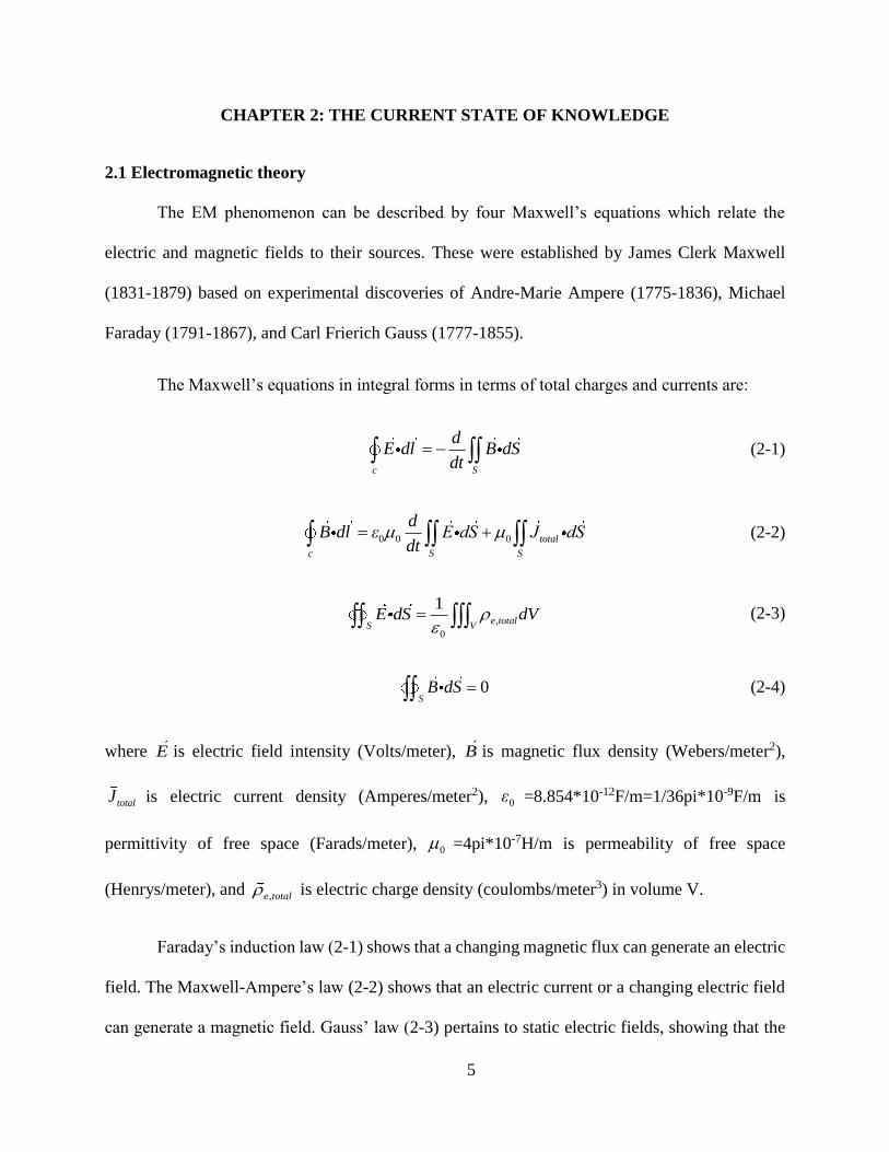
The Maxwell’s equations in integral forms in terms of total charges and currents are:
c S
dE dl B dS
dt (2-1)
0 0 0 total
c S S
dB dl ε E dS J dS
dt (2-2)
,
0
1e total
S VE dS dV
(2-3)
0S
B dS (2-4)
where E is electric field intensity (Volts/meter), B is magnetic flux density (Webers/meter2),
totalJ is electric current density (Amperes/meter2), 0ε =8.854*10-12F/m=1/36pi*10-9F/m is
permittivity of free space (Farads/meter), 0 =4pi*10-7H/m is permeability of free space
(Henrys/meter), and ,e total is electric charge density (coulombs/meter3) in volume V.
Faraday’s induction law (2-1) shows that a changing magnetic flux can generate an electric
field. The Maxwell-Ampere’s law (2-2) shows that an electric current or a changing electric field
can generate a magnetic field. Gauss’ law (2-3) pertains to static electric fields, showing that the
Page 12
6
electric field lines originate from positive charges and terminate at negative charges. Gauss’ law
for magnetism (2-4) shows that magnetic flux lines don’t have origins and must form a circle.
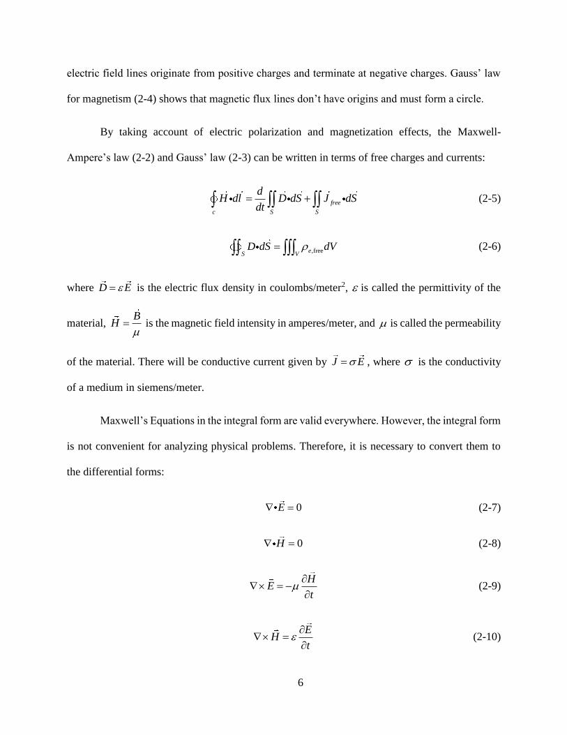
By taking account of electric polarization and magnetization effects, the Maxwell-
Ampere’s law (2-2) and Gauss’ law (2-3) can be written in terms of free charges and currents:
free
c S S
dH dl D dS J dS
dt (2-5)
,freee
S VD dS dV (2-6)
where D E is the electric flux density in coulombs/meter2, is called the permittivity of the
material, B
H
is the magnetic field intensity in amperes/meter, and is called the permeability
of the material. There will be conductive current given by J E , where is the conductivity
of a medium in siemens/meter.
Maxwell’s Equations in the integral form are valid everywhere. However, the integral form
is not convenient for analyzing physical problems. Therefore, it is necessary to convert them to
the differential forms:
0E (2-7)
0H (2-8)
H
Et
(2-9)
E
Ht
(2-10)
Page 13
7
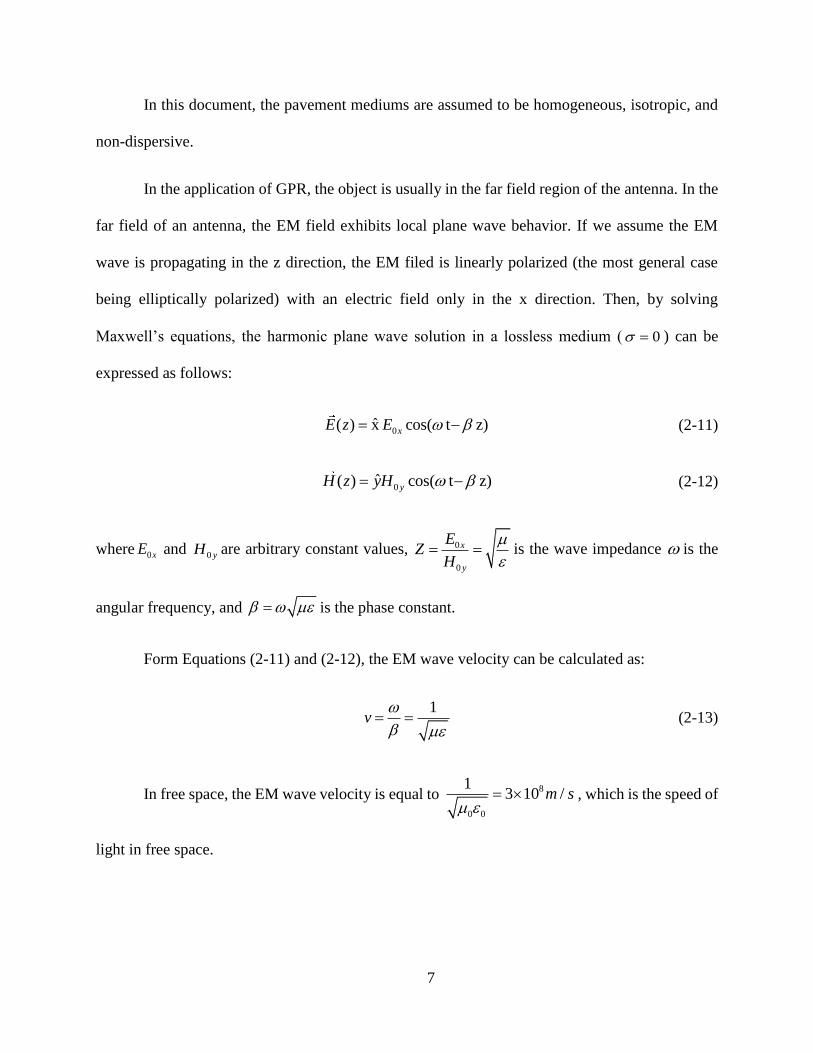
In this document, the pavement mediums are assumed to be homogeneous, isotropic, and
non-dispersive.
In the application of GPR, the object is usually in the far field region of the antenna. In the
far field of an antenna, the EM field exhibits local plane wave behavior. If we assume the EM
wave is propagating in the z direction, the EM filed is linearly polarized (the most general case
being elliptically polarized) with an electric field only in the x direction. Then, by solving
Maxwell’s equations, the harmonic plane wave solution in a lossless medium ( 0 ) can be
expressed as follows:
0ˆ( ) x cos( t z)xE z E (2-11)
0ˆ( ) cos( t z)yH z yH (2-12)
where 0xE and 0 yH are arbitrary constant values, 0
0
x
y
EZ
H
is the wave impedance is the
angular frequency, and is the phase constant.
Form Equations (2-11) and (2-12), the EM wave velocity can be calculated as:
1
v
(2-13)
In free space, the EM wave velocity is equal to 8
0 0
13 10 /m s
, which is the speed of
light in free space.
Page 14
8
In general, the electric permittivity and magnetic permeability of a material can be
expressed as ratio relative to the permittivity and permeability of space: 0
r
,
0
r
. The
relative permeability and relative permittivity (or dielectric constant) are called r and r ,
respectively.
If the plane wave is normally incident on an interface of medium 1 and medium 2, the
reflection coefficient R and transmission coefficient T are:
2 1
2 1
R
(2-14)
2
2 1
2T
(2-15)
where 1 1 1/ and 2 2 2/ are the intrinsic impedance of medium 1 and medium 2,
respectively. This is Snell’s law of reflection and transmission in the normal incident case. From
Equations (2-14) and (2-15), we can see if medium 1 and medium 2 are the same, then R=0 and
T=1, which shows that there is no reflection. If medium 2 is a perfect conductor, then 2 0 , R
= -1, and T = 0, meaning that all of the EM waves are flipped and reflected back.
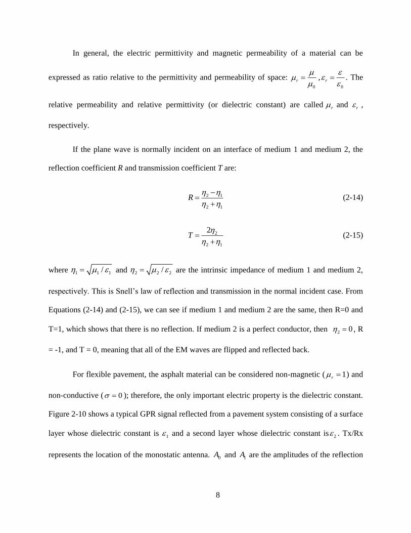
For flexible pavement, the asphalt material can be considered non-magnetic ( 1r ) and
non-conductive ( 0 ); therefore, the only important electric property is the dielectric constant.
Figure 2-10 shows a typical GPR signal reflected from a pavement system consisting of a surface
layer whose dielectric constant is 1 and a second layer whose dielectric constant is 2 . Tx/Rx
represents the location of the monostatic antenna. 0A and 1A are the amplitudes of the reflection
Page 15
9
from the surface and the bottom of the surface layer, respectively. According to Equation (2-14),
the dielectric constant of the surface layer is:
2
0
10
1
1
p
p
A
A
A
A
(2-16)
where 𝐴𝑝 is the amplitude of the reflected signal collected over a copper plate placed on the
pavement surface, which can be considered a perfect reflector.
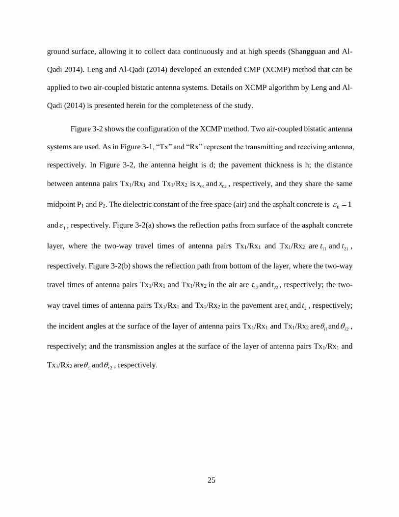
Figure 2-1. Typical GPR signal reflected from a pavement system (Zhao et al. 2015)
Knowing the dielectric constant of the surface layer, the thickness of the surface layer can
be calculated using the two-way travel time method:
2
v th
(2-17)
Page 16
10
where h is the layer thickness, t is the EM wave two-way travel time within the surface layer,
/ rv c is the speed of EM wave, c is the speed of light in free space (3 × 10⁸m/s), and r is
the dielectric constant of the surface layer.
The surface reflection and two-way travel time method provide an easy way to obtain the
dielectric constant of pavement and the thickness of the pavement layer. However, the reflection
amplitude can easily be affected by many factors, such as the surface moisture, temperature,
instability of the GPR system, and environment electric noise. Therefore, the resulting dielectric
constant and layer thickness may not be accurate enough. One possible solution is to calibrate the
dielectric constant of pavement: that is, take cores of pavement and back-calculate the dielectric
constant with obtained two-way travel time. However, this method is destructive and not preferred.
In this study, another algorithm – the common midpoint method – is used as an alternative to obtain
the dielectric constant and layer thickness. This method can provide better accuracy compared to
surface reflection and two-way travel time method without the need of calibration with cores.
2.2 Fundamental of GPR
Electrical signals are transmitted via transmission line or through empty space. Antennas
are essentially transducers that can convert electrical signals from transmission lines to empty
space, or vice versa. According to IEEE, an antenna is defined as “that part of transmitting or
receiving system that is designed to radiate or to receive electromagnetic waves” (IEEE 1993).
Ground penetration radar, in contrast, is a type of radar whose purpose is to locate targets or
interfaces buried with earth material (Daniels 2005).
Page 17
11
2.2.1 Air coupled horn antenna
One of the most popular GPR systems is the air-coupled system with horn antennas. Figure
2-2 shows a typical vehicle-mounted air-coupled GPR system. The two orange boxes are two horn
antennas with a 2GHz central frequency, and are manufactured by Geophysical Survey Systems,
Inc. (GSSI). There is a control unit called SIR20 that sends a signal to the antennas during GPR
surveys. There is also a distance measuring instrument (DMI) mounted on the back wheel of the
van to collect distance information or a GPS system. The GPR control unit and DMI system are
shown in Figure 2-3. The air-coupled antenna allows for the collection of GPR data on pavement
at highway speeds. Another advantage of this GPR system is that the horn antenna is a type of
aperture antenna (i.e., an antenna that has a physical aperture through which EM waves flow) that
has gains larger than 15 dB, which implies very good directivity (Stutzman and Thiele 2012).
Figure 2-2. A vehicle-mounted air-coupled GPR system
Page 18
12
Figure 2-3. GPR system control unit – SIR20 and DMI
2.2.2 Ultra wide band bowtie antenna
Resolution describes the ability of a signal to distinguish adjacent pulses. For example, an
EM wave with a shorter wavelength, or higher frequency, could distinguish objects with smaller
distances; therefore a signal with higher frequency usually has a greater resolution than a low
frequency signal. The Rayleigh resolution criteria, proposed by Lord Rayleigh (Culick 1987), is
the most common criteria for resolution. The one dimensional Rayleigh resolution of a signal is
the width of a pulse, which is defined as the distance between the maximum point of the pulse and
the first zero point of the pulse. A band pass filter usually decreases the resolution of a signal.
A horn antenna usually has a moderate bandwidth, or range of operation frequency. In civil
engineering applications where the target is deep, such as with ancient archeological structures,
low frequency antennas are desirable, due to their larger penetration depth; while in applications
at near surface levels, such as pavement inspection, higher frequency antennas are superior since
they can provide a better time domain resolution. In line with this, a broadband antenna could
better satisfy the requirement. A broadband antenna has a pattern, gain, and impedance nearly
Page 19
13
constant over a wide frequency range, because it has an active region that relocates on the antenna
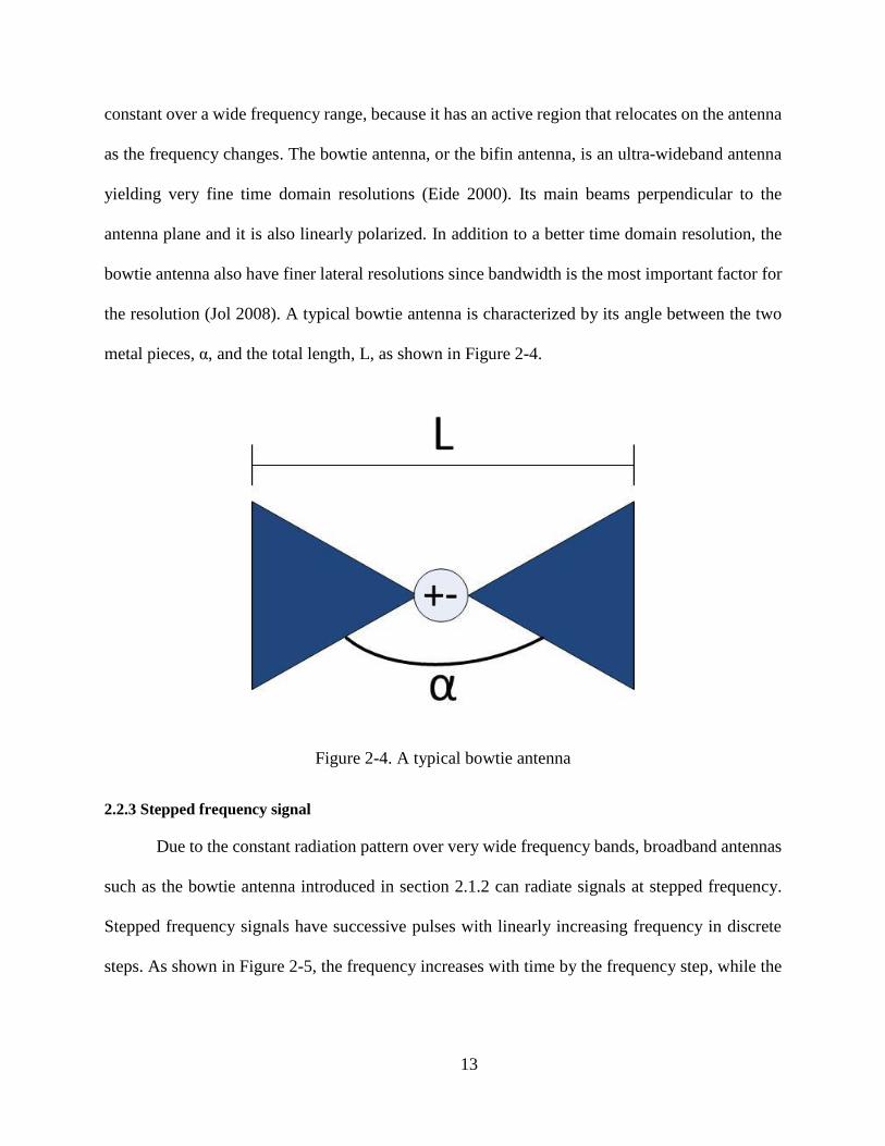
as the frequency changes. The bowtie antenna, or the bifin antenna, is an ultra-wideband antenna
yielding very fine time domain resolutions (Eide 2000). Its main beams perpendicular to the
antenna plane and it is also linearly polarized. In addition to a better time domain resolution, the
bowtie antenna also have finer lateral resolutions since bandwidth is the most important factor for
the resolution (Jol 2008). A typical bowtie antenna is characterized by its angle between the two
metal pieces, α, and the total length, L, as shown in Figure 2-4.
Figure 2-4. A typical bowtie antenna
2.2.3 Stepped frequency signal
Due to the constant radiation pattern over very wide frequency bands, broadband antennas
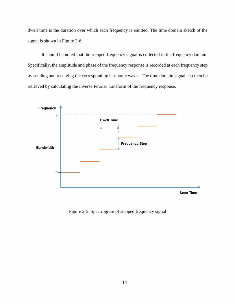
such as the bowtie antenna introduced in section 2.1.2 can radiate signals at stepped frequency.
Stepped frequency signals have successive pulses with linearly increasing frequency in discrete
steps. As shown in Figure 2-5, the frequency increases with time by the frequency step, while the
Page 20
14
dwell time is the duration over which each frequency is emitted. The time domain sketch of the
signal is shown in Figure 2-6.
It should be noted that the stepped frequency signal is collected in the frequency domain.
Specifically, the amplitude and phase of the frequency response is recorded at each frequency step
by sending and receiving the corresponding harmonic waves. The time domain signal can then be
retrieved by calculating the inverse Fourier transform of the frequency response.
Figure 2-5. Spectrogram of stepped frequency signal
Page 21
15
Figure 2-6. Time domain waveform of stepped frequency signal
With increased dwell time, a better signal to noise ratio (SNR) can be obtained. However,
due to the long dwell time, the survey speed of a single stepped frequency system will be slower
than in a pulsed system.
2.2.4 Antenna array
An antenna array is a combination of multiple antenna elements. During data collection,
electric signals are simultaneously transmitted through all elements of the array, and the reflected
signals are also simultaneously received by all elements of the array. The first popular antenna
array was the Yagi antenna, invented in 1926 by Shintaro Uda and Hidetsugu Yagi (Uda 1925),
and was widely used during World War II. Arrays are popular since, unlike a single antenna, their
radiation pattern can be controlled by adjusting the spacing and phasing of each array element.
Page 22
16
An antenna array can be characterized by the radiation pattern of a single element, i.e. the
element pattern, and by the radiation pattern of the array if its actual elements are replaced by
isotropic point sources. The latter is defined as the array factor. The total pattern of the array is
then the product of the array factor and element pattern.
The type of array element is determined by the application of the antenna. For example, a
horn antenna array can provide moderate bandwidth and need fewer array elements but the number
of scans is limited due to wide element spacing. A bowtie antenna element, on the other hand, has
a wide beam, simple structure, and a broad bandwith (Stutzman and Thiele 2012).
A synthetic aperture radar (SAR) is a single antenna moving from position to position, and
is therefore superficially similar to an antenna array (Blahut 2004). Unlike a real antenna array,
the antenna sends the pulse and records the reflection at each position one at a time. Since the
antenna is transmitting and receiving while moving, the EM wave is doppler-shifted. It should be
noted that a SAR can give less information than a real antenna array since it misses the information
when a signal is transmitted and received by two different antenna elements.
2.2.5 3-D GPR
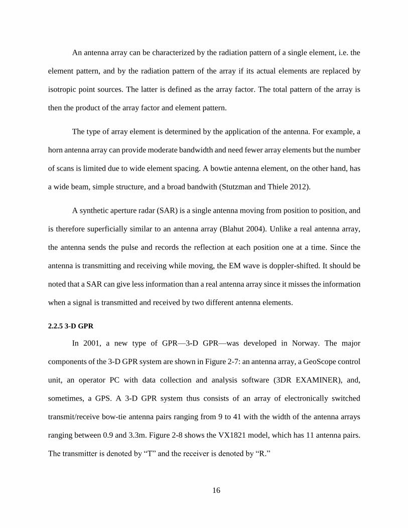
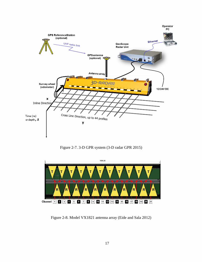
In 2001, a new type of GPR—3-D GPR—was developed in Norway. The major
components of the 3-D GPR system are shown in Figure 2-7: an antenna array, a GeoScope control
unit, an operator PC with data collection and analysis software (3DR EXAMINER), and,
sometimes, a GPS. A 3-D GPR system thus consists of an array of electronically switched
transmit/receive bow-tie antenna pairs ranging from 9 to 41 with the width of the antenna arrays
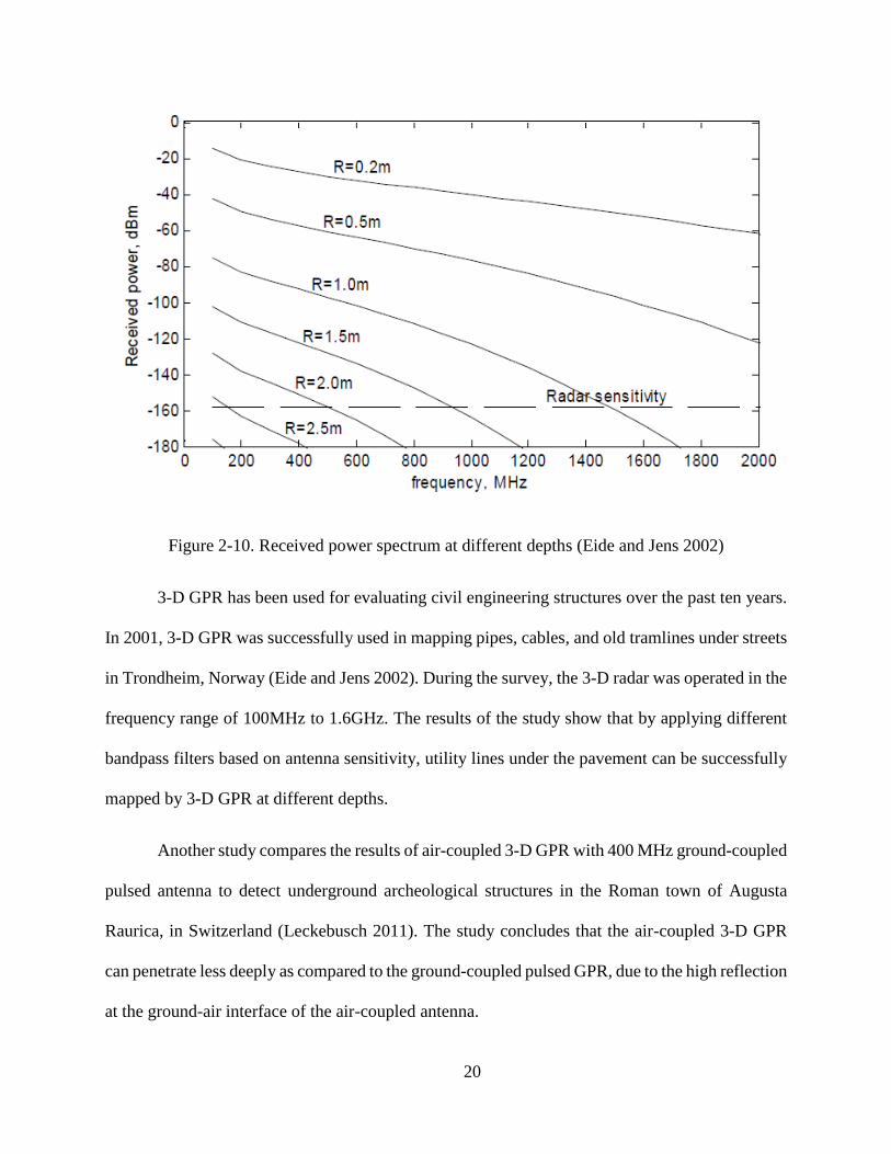
ranging between 0.9 and 3.3m. Figure 2-8 shows the VX1821 model, which has 11 antenna pairs.
The transmitter is denoted by “T” and the receiver is denoted by “R.”
Page 23
17
Figure 2-7. 3-D GPR system (3-D radar GPR 2015)
Figure 2-8. Model VX1821 antenna array (Eide and Sala 2012)
Page 24
18
The antenna element used in the 3-D GPR is a bowtie antenna with frequency ranges from
200 MHz – 3 GHz. The simulated radiation patterns of this kind of bowtie antenna at different
frequency levels are shown in Figure 2-9.
Figure 2-9. Simulated Radiation pattern of bowtie antenna (Eide and Sala 2012)
2.2.6 Application of 3-D GPR
It is known that EM waves can be reflected from local scatterers such as aggregate and air
voids in asphalt pavement. Depending on the electrical size (size in terms of EM wave length) of
the scatter, the EM scattering phenomenon can be different: if the scatterers are electrically small,
the scattering effect is Rayleigh scattering; if the size of the scatterers are comparable to the EM
wavelength, the scattering effect is in Mie scattering domain (Chuang 2009). For example, for a
2GHz horn antenna which is widely used in pavement surveys, the EM wavelength in free space
is around 0.016m and the scattering effect in asphalt pavement is more significant than low
frequency EM waves. At the same time, a high frequency antenna usually has a shorter pulse length
in the time domain, which gives better time domain resolution. Therefore, there is a tradeoff
between the penetration depth and the resolution: high frequency waves have shallow penetration
depths and better resolution at the near surface area, while low frequency wavelengths are much
Page 25
19
larger than the scale of pavement scatterer, allowing them to penetrate deeper into the ground but
with lower resolution.
This is not a problem when the GPR survey is concentrated near the surface, such as in
asphalt pavement surveys; however, if a complete survey is undertaken through the depths ranging
from the surface to several meters deep, the use of a single frequency antenna can be problematic
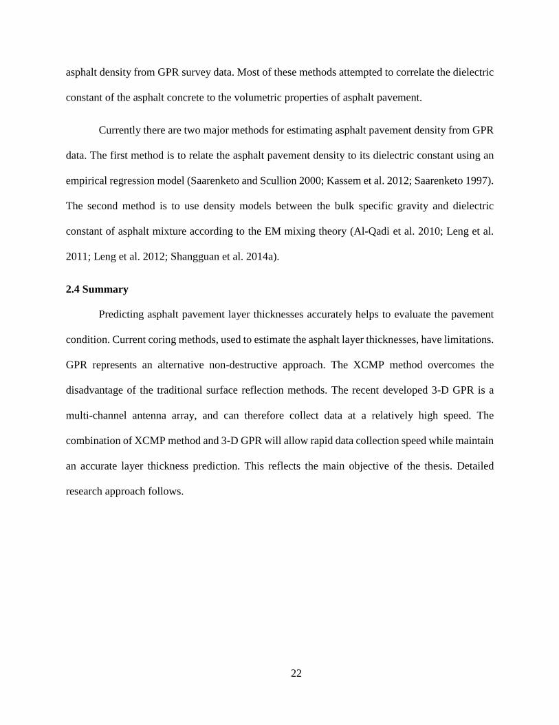
for the aforementioned reasons. Figure 2-10 shows the power received by a GPR antenna versus
frequency at different depths. The dotted line represents the GPR sensitivity line, below which the
EM signal power is too low for the receiver to sense. It is shown that at depth of 0.2m, signals at
all frequencies can get strong reflected power. As the depth increases, only the low frequency
portion of the spectrum is above the GPR sensitivity. This is consistent with the conclusion that
the GPR is sensitive to each frequency only above a particular depth. Therefore, in order to obtain
the most accurate data at each depth, one should eliminate the high frequency component in the
spectrum that would otherwise produce only noise at large depths. In light of this, the ultra-wide
band 3-D radar can be employed to generate 2D profiles at different depths.
Page 26
20
Figure 2-10. Received power spectrum at different depths (Eide and Jens 2002)
3-D GPR has been used for evaluating civil engineering structures over the past ten years.
In 2001, 3-D GPR was successfully used in mapping pipes, cables, and old tramlines under streets
in Trondheim, Norway (Eide and Jens 2002). During the survey, the 3-D radar was operated in the
frequency range of 100MHz to 1.6GHz. The results of the study show that by applying different
bandpass filters based on antenna sensitivity, utility lines under the pavement can be successfully
mapped by 3-D GPR at different depths.
Another study compares the results of air-coupled 3-D GPR with 400 MHz ground-coupled
pulsed antenna to detect underground archeological structures in the Roman town of Augusta
Raurica, in Switzerland (Leckebusch 2011). The study concludes that the air-coupled 3-D GPR
can penetrate less deeply as compared to the ground-coupled pulsed GPR, due to the high reflection
at the ground-air interface of the air-coupled antenna.
Page 27
21
2.3 GPR applications on asphalt pavement
2.3.1 Layer thickness estimation
The most prevalent application of GPR on asphalt pavement is the estimation of layer
thickness, due to the straightforwardness of the surface reflection and the two-way travel time
method. Many studies have examined using GPR for this application. Using the two-way travel
time method, Al-Qadi et al. (2003) reported a mean thickness error of 2.9% for asphalt pavement
layers ranging between 100 mm and 250 mm in thickness on a newly built test section of Route
288 in Richmond, Virginia, United States. Lahouar et al. (2002) analyzed GPR data collected from
interstate highway I-81 using a kind of multi-offset measurement method – the common midpoint
method (CMP) –reporting a thickness error ranging from 1% to 15% with a mean error of 6.8%.
Liu et al. (2014) applied a similar CMP method and envelope velocity spectrum analysis to GPR
data to measure the dielectric permittivity and thickness of snow and ice cover on a brackish lagoon,
with good accuracy. Liu and Sato (2014) used another multi-offset measurement method – the
common source method – for asphalt layer thickness and EM wave velocity estimation. In the
study they first designed a Vivaldi antenna array and then calibrated the phase center using a
gypsum model. The results from their field experiment shows that the error of asphalt layer
thickness estimation is less than 6mm (10%). The Wide Angle Refraction and Reflection (WARR)
method can also be used to measure the EM wave velocity within the surface layer and therefore
the dielectric constant and thickness of the surface layer (Huisman et al. 2001).
2.3.2 Asphalt pavement density estimation
Asphalt pavement density is another important factor that influences the performance and
service life of the pavement (Roberts et al. 1996). There have been many studies trying to predict
Page 28
22
asphalt density from GPR survey data. Most of these methods attempted to correlate the dielectric
constant of the asphalt concrete to the volumetric properties of asphalt pavement.
Currently there are two major methods for estimating asphalt pavement density from GPR
data. The first method is to relate the asphalt pavement density to its dielectric constant using an
empirical regression model (Saarenketo and Scullion 2000; Kassem et al. 2012; Saarenketo 1997).
The second method is to use density models between the bulk specific gravity and dielectric
constant of asphalt mixture according to the EM mixing theory (Al-Qadi et al. 2010; Leng et al.
2011; Leng et al. 2012; Shangguan et al. 2014a).
2.4 Summary
Predicting asphalt pavement layer thicknesses accurately helps to evaluate the pavement
condition. Current coring methods, used to estimate the asphalt layer thicknesses, have limitations.
GPR represents an alternative non-destructive approach. The XCMP method overcomes the
disadvantage of the traditional surface reflection methods. The recent developed 3-D GPR is a
multi-channel antenna array, and can therefore collect data at a relatively high speed. The
combination of XCMP method and 3-D GPR will allow rapid data collection speed while maintain
an accurate layer thickness prediction. This reflects the main objective of the thesis. Detailed
research approach follows.
Page 29
23
CHAPTER 3: RESEARCH APPROACH
3.1 Extended CMP method
Multi-offset methods were originally used in seismic migration to measure seismic wave
velocity (Yilmaz 2008). The common source method and common midpoint (CMP) method are
the two common multi-offset techniques (Schneider 1984). The CMP method has been recently
used to calculate the EM wave velocity within asphalt concrete pavement layers (Lahouar 2002).
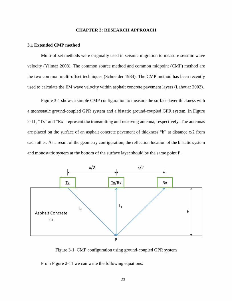
Figure 3-1 shows a simple CMP configuration to measure the surface layer thickness with
a monostatic ground-coupled GPR system and a bistatic ground-coupled GPR system. In Figure
2-11, “Tx” and “Rx” represent the transmitting and receiving antenna, respectively. The antennas
are placed on the surface of an asphalt concrete pavement of thickness “h” at distance x/2 from
each other. As a result of the geometry configuration, the reflection location of the bistatic system
and monostatic system at the bottom of the surface layer should be the same point P.
Figure 3-1. CMP configuration using ground-coupled GPR system
From Figure 2-11 we can write the following equations:
Page 30
24
1 2vt h (3-1)
2
2
2 22
xvt h
(3-2)
where 1t is the two way-travel time from point P of the monostatic system and 2t is the two-way
travel time from point P of the bistatic system. From Equations (3-1) and (3-2), the layer thickness
h and EM wave velocity can be calculated:
2 2
2 1
xv
t t
(3-3)
1
2 2
2 1
2xth
t t
(3-4)
The dielectric constant of the asphalt concrete can then be obtained from1
cv
.
Therefore, once the two-way travel times of both antenna systems are obtained from the
collected signals, the dielectric constant as well as the layer thickness can be obtained. This
assumes that the pavement is thick enough, or the frequency band of the EM wave is wide enough,
and that the two pulses reflected from the surface and the bottom of the layer can be
distinguished—i.e., there is enough time resolution. Otherwise, super resolution techniques such
as deconvolution need to be used to distinguish the overlapping pulses (Zhao et al. 2015; La
Bastard et al. 2012).
In the previous discussed CMP method, we assume that the two antenna systems are all
ground-coupled systems. However, in this study, the available 3-D GPR is an air-coupled system.
One of the advantages of an air-coupled system is that it doesn’t require direct contact with the
Page 31
25
ground surface, allowing it to collect data continuously and at high speeds (Shangguan and Al-
Qadi 2014). Leng and Al-Qadi (2014) developed an extended CMP (XCMP) method that can be
applied to two air-coupled bistatic antenna systems. Details on XCMP algorithm by Leng and Al-
Qadi (2014) is presented herein for the completeness of the study.
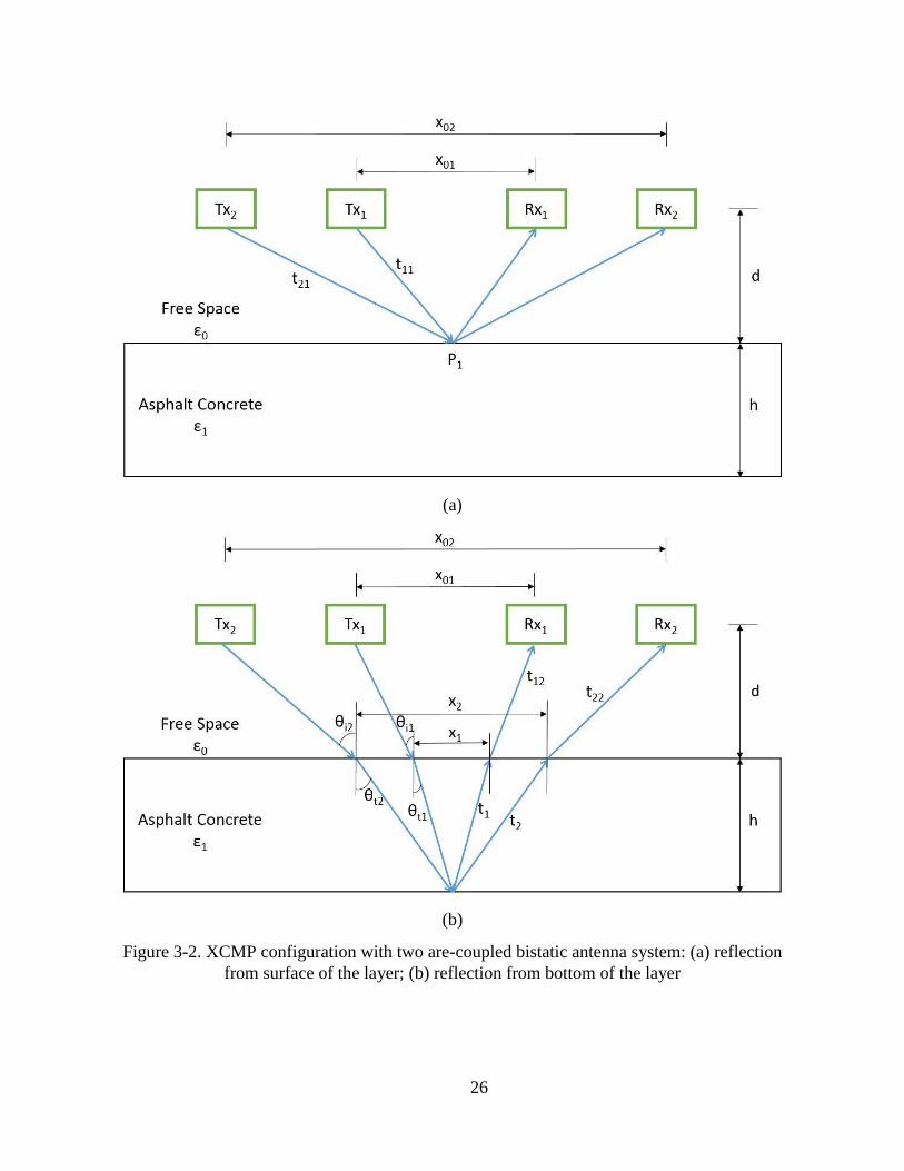
Figure 3-2 shows the configuration of the XCMP method. Two air-coupled bistatic antenna
systems are used. As in Figure 3-1, “Tx” and “Rx” represent the transmitting and receiving antenna,
respectively. In Figure 3-2, the antenna height is d; the pavement thickness is h; the distance
between antenna pairs Tx1/Rx1 and Tx1/Rx2 is 01x and 02x , respectively, and they share the same
midpoint P1 and P2. The dielectric constant of the free space (air) and the asphalt concrete is 0 1
and 1 , respectively. Figure 3-2(a) shows the reflection paths from surface of the asphalt concrete
layer, where the two-way travel times of antenna pairs Tx1/Rx1 and Tx1/Rx2 are 11t and 21t ,
respectively. Figure 3-2(b) shows the reflection path from bottom of the layer, where the two-way
travel times of antenna pairs Tx1/Rx1 and Tx1/Rx2 in the air are 12t and 22t , respectively; the two-
way travel times of antenna pairs Tx1/Rx1 and Tx1/Rx2 in the pavement are 1t and 2t , respectively;
the incident angles at the surface of the layer of antenna pairs Tx1/Rx1 and Tx1/Rx2 are 1i and 2i ,
respectively; and the transmission angles at the surface of the layer of antenna pairs Tx1/Rx1 and
Tx1/Rx2 are 1t and 2t , respectively.
Page 32
26
(a)
(b)
Figure 3-2. XCMP configuration with two are-coupled bistatic antenna system: (a) reflection
from surface of the layer; (b) reflection from bottom of the layer
Page 33
27
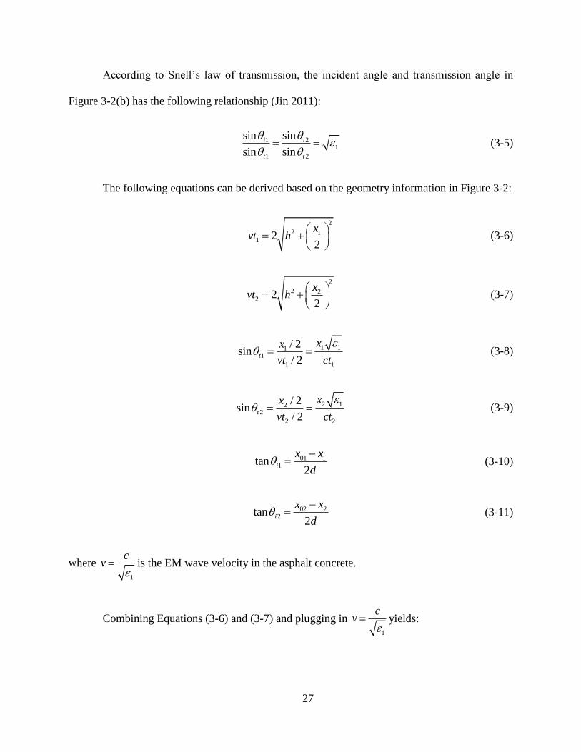
According to Snell’s law of transmission, the incident angle and transmission angle in
Figure 3-2(b) has the following relationship (Jin 2011):
1 21
1 2
sin sin
sin sin
i i
t t
(3-5)
The following equations can be derived based on the geometry information in Figure 3-2:
2
2 11 2
2
xvt h
(3-6)
2
2 22 2
2
xvt h
(3-7)
1 111
1 1
/ 2sin
/ 2t
xx
vt ct
(3-8)
2 122
2 2
/ 2sin
/ 2t
xx
vt ct
(3-9)
01 11tan
2i
x x
d
(3-10)
02 22tan
2i
x x
d
(3-11)
where 1
cv
is the EM wave velocity in the asphalt concrete.
Combining Equations (3-6) and (3-7) and plugging in 1
cv
yields:
Page 34
28
2 2 2
2 11 2 2
2 1
(t t )c
x x
(3-12)
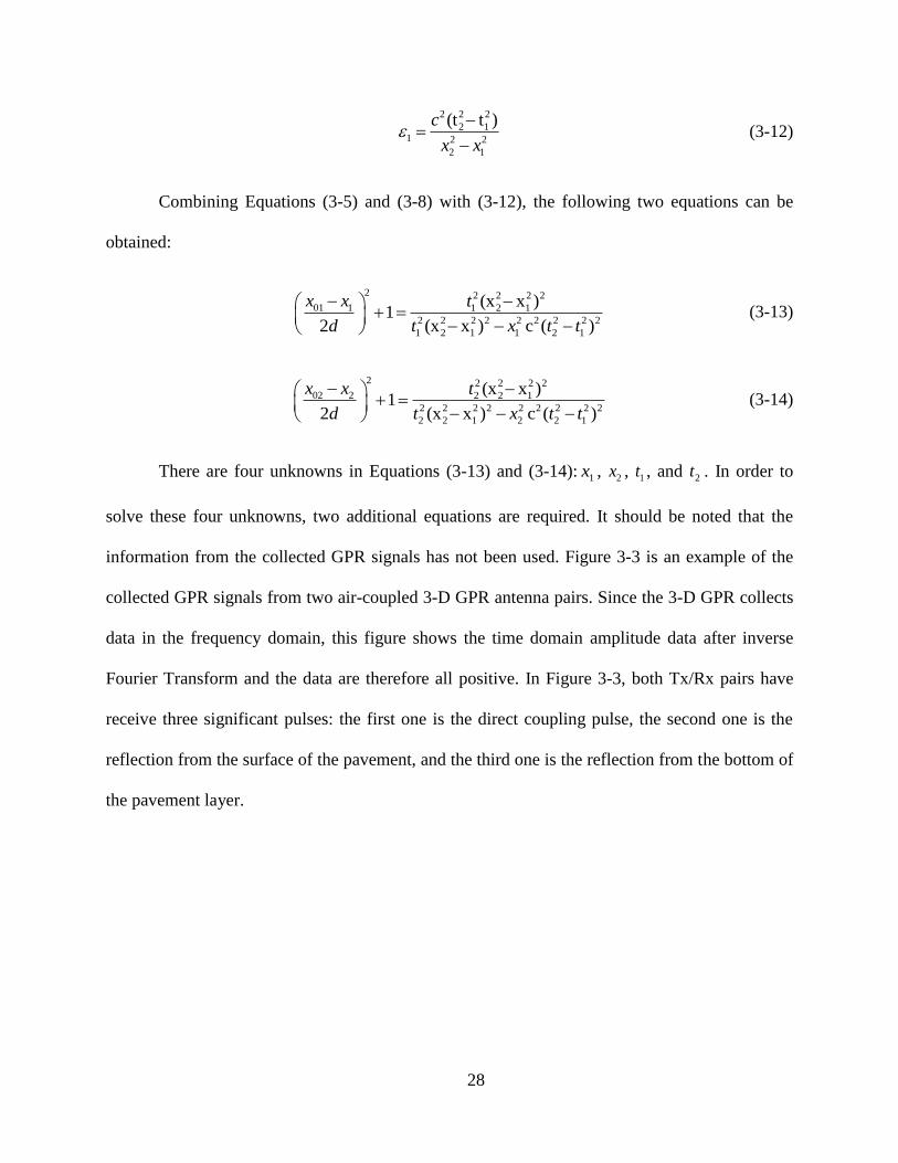
Combining Equations (3-5) and (3-8) with (3-12), the following two equations can be
obtained:
2 2 2 2 2
01 1 1 2 1
2 2 2 2 2 2 2 2 2
1 2 1 1 2 1
(x x )1
2 (x x ) c ( )
x x t
d t x t t
(3-13)
2 2 2 2 2
02 2 2 2 1
2 2 2 2 2 2 2 2 2
2 2 1 2 2 1
(x x )1
2 (x x ) c ( )
x x t
d t x t t
(3-14)
There are four unknowns in Equations (3-13) and (3-14): 1x , 2x , 1t , and 2t . In order to
solve these four unknowns, two additional equations are required. It should be noted that the
information from the collected GPR signals has not been used. Figure 3-3 is an example of the
collected GPR signals from two air-coupled 3-D GPR antenna pairs. Since the 3-D GPR collects
data in the frequency domain, this figure shows the time domain amplitude data after inverse
Fourier Transform and the data are therefore all positive. In Figure 3-3, both Tx/Rx pairs have
receive three significant pulses: the first one is the direct coupling pulse, the second one is the
reflection from the surface of the pavement, and the third one is the reflection from the bottom of
the pavement layer.
Page 35
29
Figure 3-3. Collected XCMP GPR signals from two air-coupled 3-D GPR antenna pairs
As shown in Figure 3-3, the time difference between the surface reflection and the
reflection at the bottom of the layer 1t and 2t can be directly obtained from the collected data,
and they can be expressed as follows:
1 12 1 11t t t t (3-15)
2 22 2 21t t t t (3-16)
where
2 2
01
11
2 / 4d xt
c
(3-17)
2 2
02
21
2 / 4d xt
c
(3-18)
Page 36
30
2 2
01 1
12
2 ( ) / 4d x xt
c
(3-19)
2 2
02 2
22
2 ( ) / 4d x xt
c
(3-20)
Therefore, the following two equations can be obtained by substituting Equations (3-17) to
(3-20) into Equations (3-15) and (3-16):
2 2 2 2
01 1 01
1 1
2 ( ) / 4 2 / 4d x x d xt t
c c
(3-21)
2 2 2 2
02 2 02
2 2
2 ( ) / 4 2 / 4d x x d xt t
c c
(3-22)
With Equations (3-13), (3-14), (3-21) and (3-22), the four unknowns 1x , 2x , 1t , and 2t can
be solved numerically using the optimization method described in Section 3.3.3. The dielectric
constant of asphalt concrete 1 and the asphalt layer thickness h can then be obtained from
Equations (3-12) and (3-6), respectively.
3.2 Experiment plan with 3-D GPR to validate XCMP method
With the XCMP method described in the previous section, Leng and Al-Qadi (2014)
successfully validated that the pulsed antenna can provide better accuracy in determining asphalt
pavement layer thickness than the surface reflection method. In that study, two air-coupled horn
antennas manufactured by Geophysical Survey Systems, Inc. (GSSI) were used (Figure 2-1). A
test site was constructed as shown in Figure 3-4.
Page 37
31
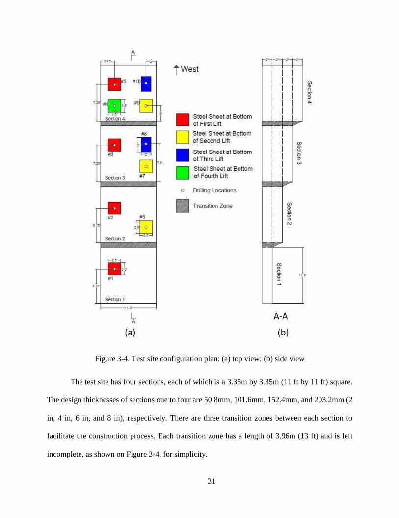
Figure 3-4. Test site configuration plan: (a) top view; (b) side view
The test site has four sections, each of which is a 3.35m by 3.35m (11 ft by 11 ft) square.
The design thicknesses of sections one to four are 50.8mm, 101.6mm, 152.4mm, and 203.2mm (2
in, 4 in, 6 in, and 8 in), respectively. There are three transition zones between each section to
facilitate the construction process. Each transition zone has a length of 3.96m (13 ft) and is left
incomplete, as shown on Figure 3-4, for simplicity.
Page 38
32
There are steel plates placed at the bottom of each asphalt lift to increase the reflection
coefficient at the bottom of the pavement, since it can then be regarded as a perfect reflector,
reflecting back all the EM wave energy. This is not necessary in practice when the dielectric
constant difference between the surface layer and the bottom layer is significant. The layout of the
steel plates is shown in Figure 3-4: section n has n steel plates embedded in the asphalt concrete at
different depths, where n=1 to 4.
This study used a DX1821 antenna array manufactured by 3D-Radar Company. Similar to
the one shown in Figure 2-7, the DX1821 system has a total of eleven bow-tie monopole transiting
antennas and eleven bow-tie monopole receiving antennas. It has a total length of 1.8m with an
effective scan width of 1.575m. Each of the bow-tie antenna has an ultra-wide frequency band
from 200MHz to 3GHz and can radiate EM signal in a stepped frequency manner, as explained in
section 2.1.3. The antenna spacing is 0.15m. A total of 21 channels could be configured arbitrarily
between one transmitting antenna and one receiving antenna (3D-Radar GPR 2015).
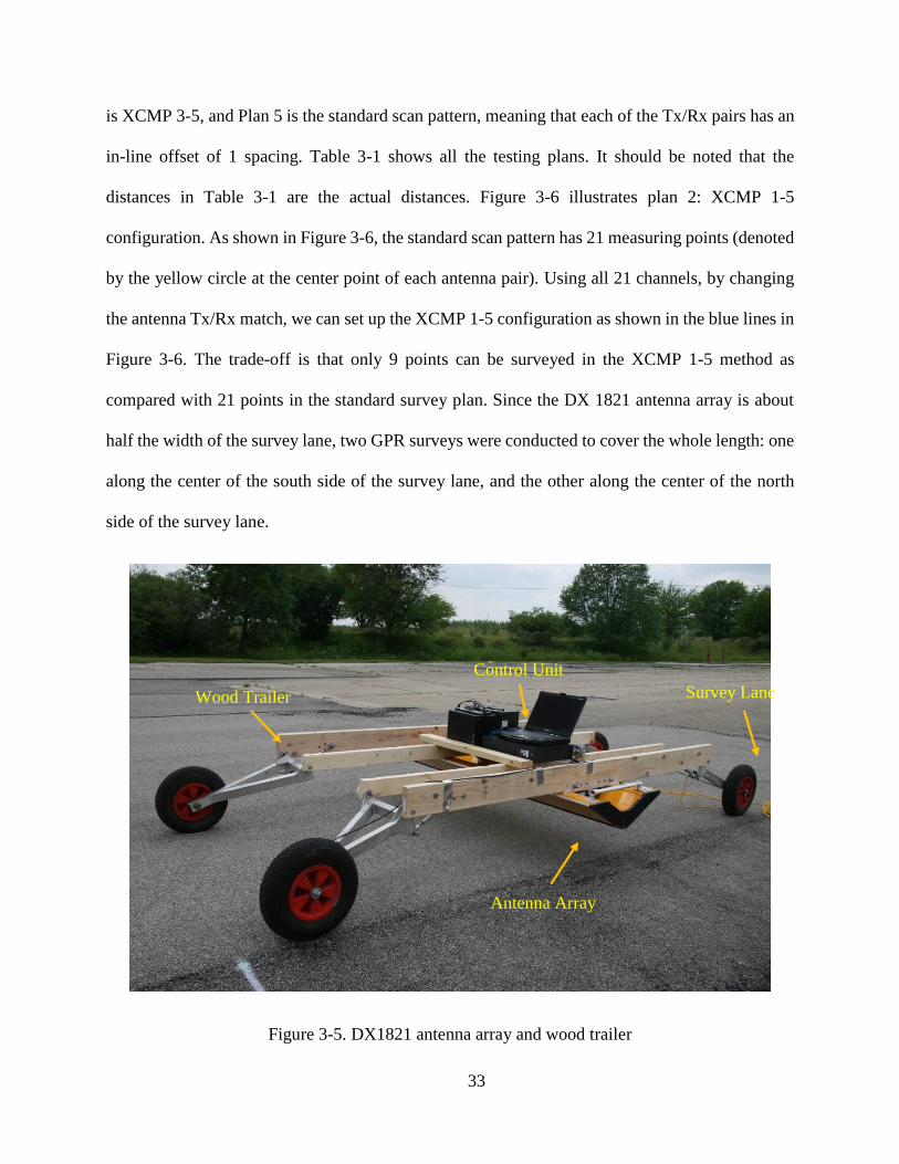
To survey the whole lane, a wood trailer was built to carry the antenna array—as shown in
Figure 3-5—together with the antenna array and control unit. After calibration, the phase center of
each bow-tie antenna was found to be 0.369m above the ground.
In order to apply the XCMP method, several different antenna scan patterns are designed
to have multiple XCMP offsets. The authors devised total five testing plans to find the best
configuration based on the results. Plan 1 is XCMP 1-3, meaning that the cross-line offset between
Tx1/Rx1 is 1 intervals, and the cross-line offset between Tx2/Rx2 is 3 intervals. “In-line” and
“cross-line” refer to the directions parallel to the survey direction and the length of the antenna
array, respectively, and the cross-line intervals and in-line intervals were 0.075m and 0.44m,
respectively, as shown in Figure 3-6. Similarly, Plan 2 is XCMP 1-5, Plan 3 is XCMP 1-7, Plan 4
Page 39
33
is XCMP 3-5, and Plan 5 is the standard scan pattern, meaning that each of the Tx/Rx pairs has an
in-line offset of 1 spacing. Table 3-1 shows all the testing plans. It should be noted that the
distances in Table 3-1 are the actual distances. Figure 3-6 illustrates plan 2: XCMP 1-5
configuration. As shown in Figure 3-6, the standard scan pattern has 21 measuring points (denoted
by the yellow circle at the center point of each antenna pair). Using all 21 channels, by changing
the antenna Tx/Rx match, we can set up the XCMP 1-5 configuration as shown in the blue lines in
Figure 3-6. The trade-off is that only 9 points can be surveyed in the XCMP 1-5 method as
compared with 21 points in the standard survey plan. Since the DX 1821 antenna array is about
half the width of the survey lane, two GPR surveys were conducted to cover the whole length: one
along the center of the south side of the survey lane, and the other along the center of the north
side of the survey lane.
Figure 3-5. DX1821 antenna array and wood trailer
Wood Trailer
Control Unit
Antenna Array
Survey Lane
Page 40
34
Table 3-1. XCMP antenna setting plans
Plan 1 2 3 4 5
Configuration XCMP 1-3 XCMP 1-5 XCMP 1-7 XCMP 3-5 Standard
Distance between
Tx/Rx pair 1 (m) 0.446 0.446 0.446 0.369 0.446
Distance between
Tx/Rx pair 2 (m) 0.369 0.578 0.685 0.578 -
Figure 3-6 DX 1821 antenna array layout, standard survey and XCMP 1-5 test configuration
After all 10 GPR surveys (2 surveys for each test plan) were completed, the collected GPR
data were converted to time domain signals and corresponding signal processing techniques were
applied (see Section 3.3). The signal directed reflected from the center of each steel plate was used
to calculate the dielectric constant and layer thickness. The signal reflected from the center of each
steel plate can be approximated found by identifying the maximum reflection amplitude.
Cores were drilled at the center of each steel plate and their thicknesses were measured in
the laboratory to provide the as-built pavement thicknesses of each section. The accuracy of the
proposed algorithm could then be evaluated (see Section 4).
Page 41
35
3.3 Signal Processing
3.3.1 3-D GPR signal characteristics
As explained in section 2.1.2, the resolution of a signal is important as it determines the
ability to distinguish adjacent pulses. Where GPR is used to determine asphalt layer thickness by
applying a two-way travel method, the time domain resolution of the GPR signal is critical, due to
the reasons explained in section 3.1. When the XCMP method is used, it is also necessary to
distinguish the reflection from the surface and the bottom of the surface layer to obtain 1t and 2t
in Equations (3-15) and (3-16). An example of the 3-D GPR signal reflected back from a two-
layered asphalt pavement system is shown in Figure 3-7. The Rayleigh resolution of the signal was
found to be 0.61ns, as shown in Figure 3-7. Therefore, if the 3-D GPR signal is normally incident
on the pavement whose dielectric is 4, the smallest thickness that can be resolved is
80.61 3 10 / 6 / 74.7ns m s mm , which about 75mm. For a GSSI 2GHz horn antenna, the
Rayleigh resolution is 0.5382ns. This shows that the pulsed horn antenna has good time domain
resolution due to its wide bandwidth.
Page 42
36
Figure 3-7. 3-D GPR signal over a two-layered asphalt pavement system
3.3.2 Whittaker–Shannon interpolation
According to section 3.1, the result of XCMP problem can be obtained by solving a set of
four non-linear equations (3-13), (3-14), (3-21) and (3-22). Numerical solutions, such as least
square solutions, are needed to solve these equations. However, such equations are not necessarily
stable, meaning that a small disturbance in the inputs ( 01x , 02x , d , 1t and 2t ) could have a huge
influence on the outputs ( 1x , 2x , 1t , and 2t ). The layout of the 3-D GPR was provided by the 3-D
Radar Company and therefore the values of 01x , 02x and d have been well calibrated to yield
sufficient accuracy. After sensitivity analysis, we also found that the output results are most
sensible to the change of 1t and 2t .
Page 43
37
Since the 3-D GPR collects signal in the frequency domain, the time domain signal is
“synthetized” by inverse Fourier transform of the frequency domain signal, and the time domain
signal sampling interval is directly related to the frequency bandwidth, according to the Discrete
Fourier Transform (DFT) property:
1
dtf
(3-23)
where dt is the time domain sampling interval and f is the upper limit of the frequency band.
For the DX1821 3-D GPR, the time domain sampling interval is 0.12207 ns, and the corresponding
upper limit of the frequency band is 8.19 GHz. Compared with the time domain sampling interval
of a 2 GHz GSSI pulsed horn antenna—which is 0.0234ns according to Zhao et al. (2015)—it is
shown that the 3-D GPR has a smaller time domain sampling interval. In other words, the
frequency band of 3-D GPR is not significantly wider than that of the 2 GHz GSSI pulsed horn
antenna. However, if we assume that the frequency content of the 3-D GPR signal above the upper
limit of the frequency band is all zero, then the time domain sampling interval of the signal can be
decreased by zero padding the frequency domain signal (Lyons 2010). The corresponding time
domain process is the Whittaker–Shannon interpolation, or the Sinc interpolation:
( ) [ ]sincn
t ndtx t x n
dt
(3-24)
where discrete time signal [ ]x n is continuous time signal ( )x t sampled at ndt , n is an integer,
sin( )sinc(x)
x
x is the sinc function, and dt is the time domain sampling interval. If the sampling
interval dt meets the Nyquist criteria—i.e. the sampling frequency 1/dt is higher than twice the
maximum frequency content of the analog signal—then Equation (3-24) can perfectly restore the
Page 44
38
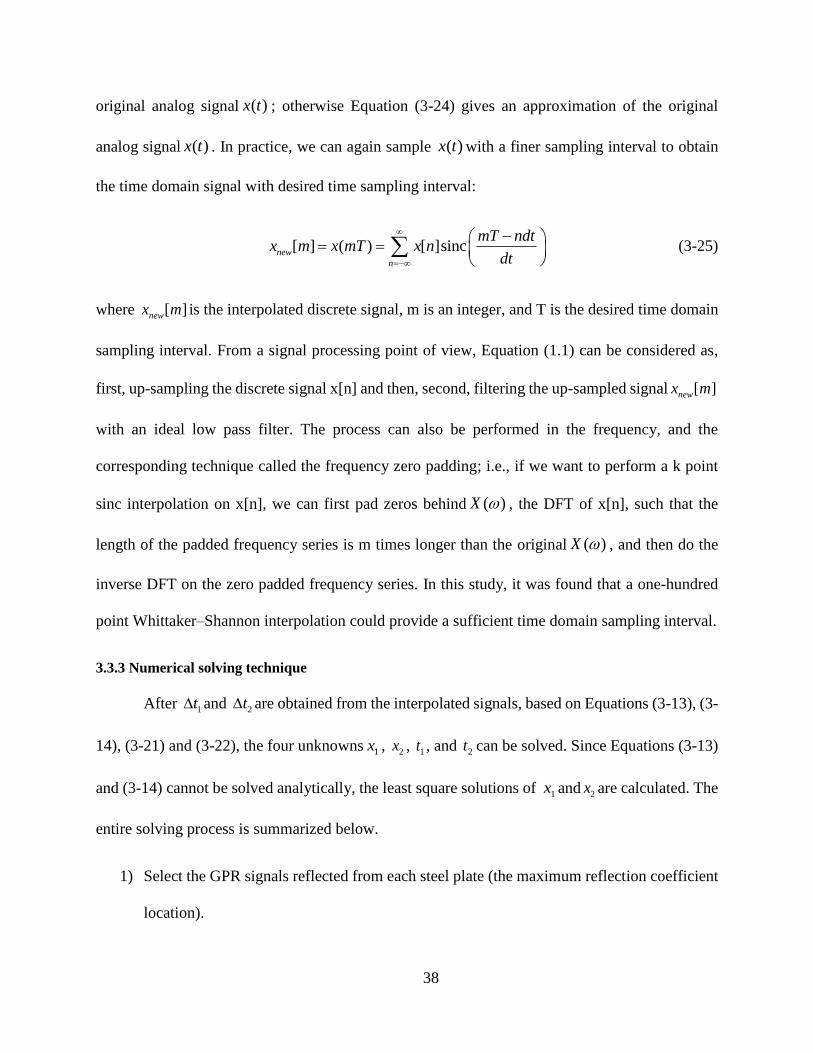
original analog signal ( )x t ; otherwise Equation (3-24) gives an approximation of the original
analog signal ( )x t . In practice, we can again sample ( )x t with a finer sampling interval to obtain
the time domain signal with desired time sampling interval:
[ ] ( ) [ ]sincnew
n
mT ndtx m x mT x n
dt
(3-25)
where [ ]newx m is the interpolated discrete signal, m is an integer, and T is the desired time domain
sampling interval. From a signal processing point of view, Equation (1.1) can be considered as,
first, up-sampling the discrete signal x[n] and then, second, filtering the up-sampled signal [ ]newx m
with an ideal low pass filter. The process can also be performed in the frequency, and the
corresponding technique called the frequency zero padding; i.e., if we want to perform a k point
sinc interpolation on x[n], we can first pad zeros behind ( )X , the DFT of x[n], such that the
length of the padded frequency series is m times longer than the original ( )X , and then do the
inverse DFT on the zero padded frequency series. In this study, it was found that a one-hundred
point Whittaker–Shannon interpolation could provide a sufficient time domain sampling interval.
3.3.3 Numerical solving technique
After 1t and 2t are obtained from the interpolated signals, based on Equations (3-13), (3-
14), (3-21) and (3-22), the four unknowns 1x , 2x , 1t , and 2t can be solved. Since Equations (3-13)
and (3-14) cannot be solved analytically, the least square solutions of 1x and 2x are calculated. The
entire solving process is summarized below.
1) Select the GPR signals reflected from each steel plate (the maximum reflection coefficient
location).
Page 45
39
2) Perform 100-points Whittaker–Shannon interpolation on each of the GPR signals.
3) From Equations (3-21) and (3-22), 1t and 2t can be expressed in terms of 1x , 2x .
Substituting 1t and 2t into Equations (3-13) and (3-14) yields two equations with two
unknowns 1x and 2x .
4) Discretize 1x and 2x with distance step of 0.001 m in the range 1 01 2 1 02(0, ), ( , )x x x x x
according to Figure 3-2(b).
5) Find the 1x and 2x , such that the residue of the Equations (3-13) and (3-14) are minimized:
1 01 2 1 02
1 2 1 2(0, ), ( , )
[ , ] arg min ([ , ])x x x x x
x x norm r r
(3-26)
where 1r and 2r are the residues of Equations (3-13) and (3-14), respectively. It should be
noted that if the minimum norm is located at the boundary of the area
1 01 2 1 02(0, ), ( , )x x x x x , the resulting 1x and 2x are not the solutions of Equations (3-13)
and (3-14).
6) Find 1t and 2t From Equations (3-21) and (3-22).
7) Find the dielectric constant of the asphalt concrete 1 from Equation (3-12).
8) Find the layer thickness h from Equation (3-6) or (3-7).
Page 46
40
CHAPTER 4: TEST RESULTS AND DISCUSSION
4.1 3-D GPR standard scan pattern results
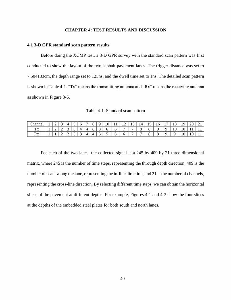
Before doing the XCMP test, a 3-D GPR survey with the standard scan pattern was first
conducted to show the layout of the two asphalt pavement lanes. The trigger distance was set to
7.504183cm, the depth range set to 125ns, and the dwell time set to 1ns. The detailed scan pattern
is shown in Table 4-1. “Tx” means the transmitting antenna and “Rx” means the receiving antenna
as shown in Figure 3-6.
Table 4-1. Standard scan pattern
Channel 1 2 3 4 5 6 7 8 9 10 11 12 13 14 15 16 17 18 19 20 21
Tx 1 2 2 3 3 4 4 8 8 6 6 7 7 8 8 9 9 10 10 11 11
Rx 1 1 2 2 3 3 4 4 5 5 6 6 7 7 8 8 9 9 10 10 11
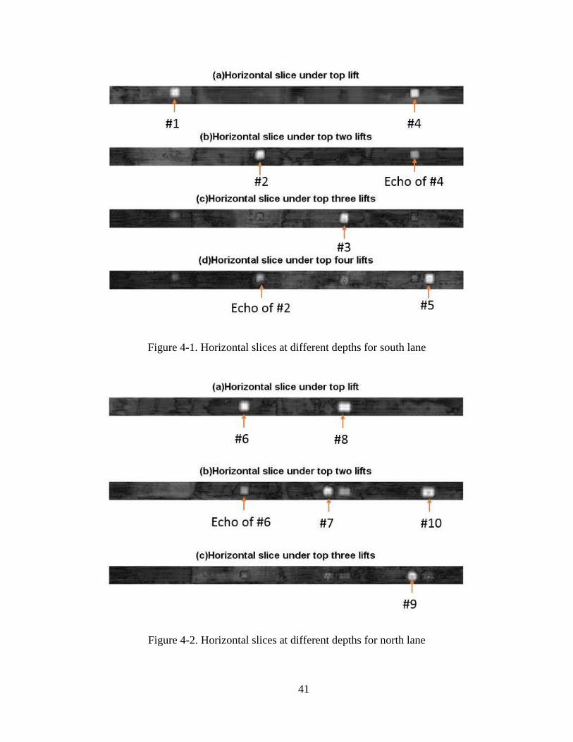
For each of the two lanes, the collected signal is a 245 by 409 by 21 three dimensional
matrix, where 245 is the number of time steps, representing the through depth direction, 409 is the
number of scans along the lane, representing the in-line direction, and 21 is the number of channels,
representing the cross-line direction. By selecting different time steps, we can obtain the horizontal
slices of the pavement at different depths. For example, Figures 4-1 and 4-3 show the four slices
at the depths of the embedded steel plates for both south and north lanes.
Page 47
41
Figure 4-1. Horizontal slices at different depths for south lane
Figure 4-2. Horizontal slices at different depths for north lane
Page 48
42
The rectangular spots in Figures 4-1 and 4-2 represent areas with very high reflection
coefficients, corresponding to the places where steel plates are embedded. Together with the steel
plate configuration shown in Figure 3-4, we can see that by selecting the GPR signals at different
horizontal slices corresponding to the depth of the steel plate, the steel plates can be clearly seen.
This shows the ability of 3-D GPR to map pavement sections accurately and rapidly. It should be
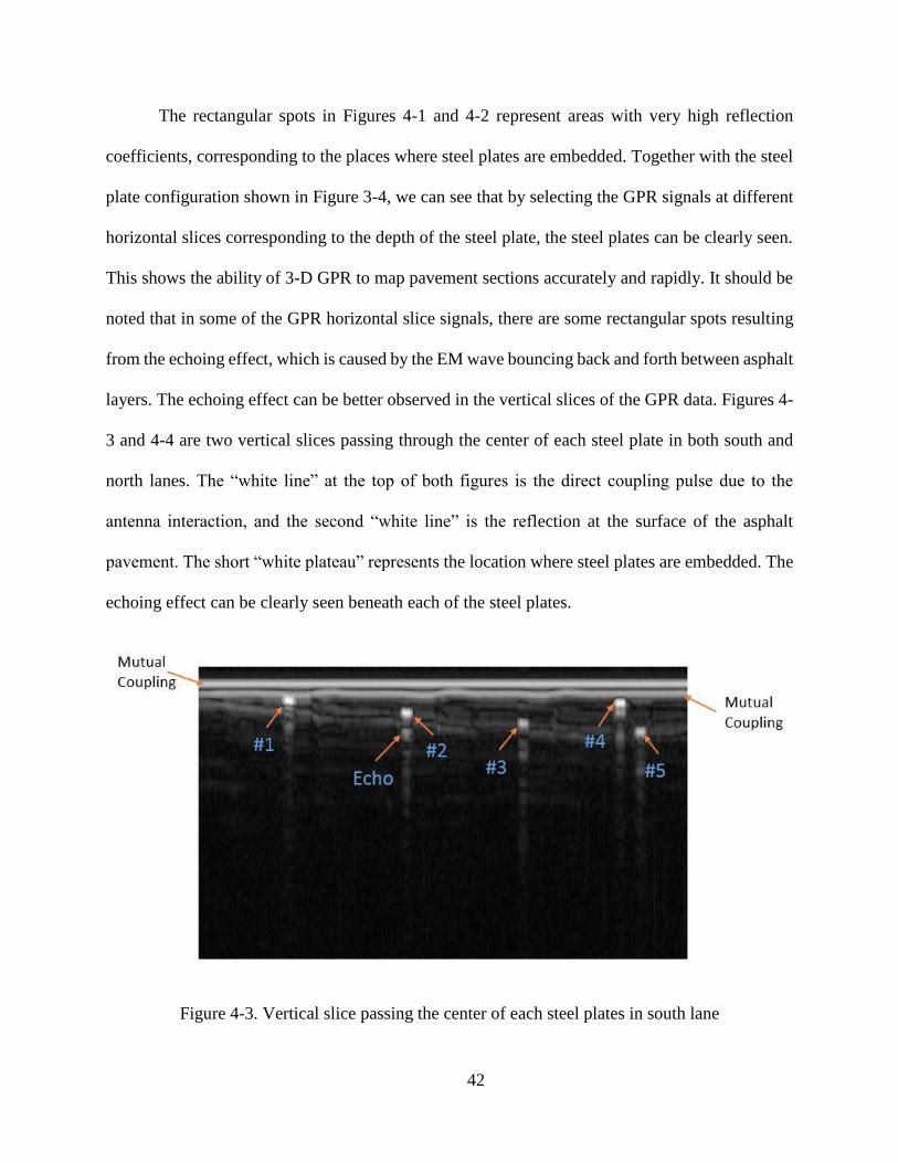
noted that in some of the GPR horizontal slice signals, there are some rectangular spots resulting
from the echoing effect, which is caused by the EM wave bouncing back and forth between asphalt
layers. The echoing effect can be better observed in the vertical slices of the GPR data. Figures 4-
3 and 4-4 are two vertical slices passing through the center of each steel plate in both south and
north lanes. The “white line” at the top of both figures is the direct coupling pulse due to the
antenna interaction, and the second “white line” is the reflection at the surface of the asphalt
pavement. The short “white plateau” represents the location where steel plates are embedded. The
echoing effect can be clearly seen beneath each of the steel plates.
Figure 4-3. Vertical slice passing the center of each steel plates in south lane
Page 49
43
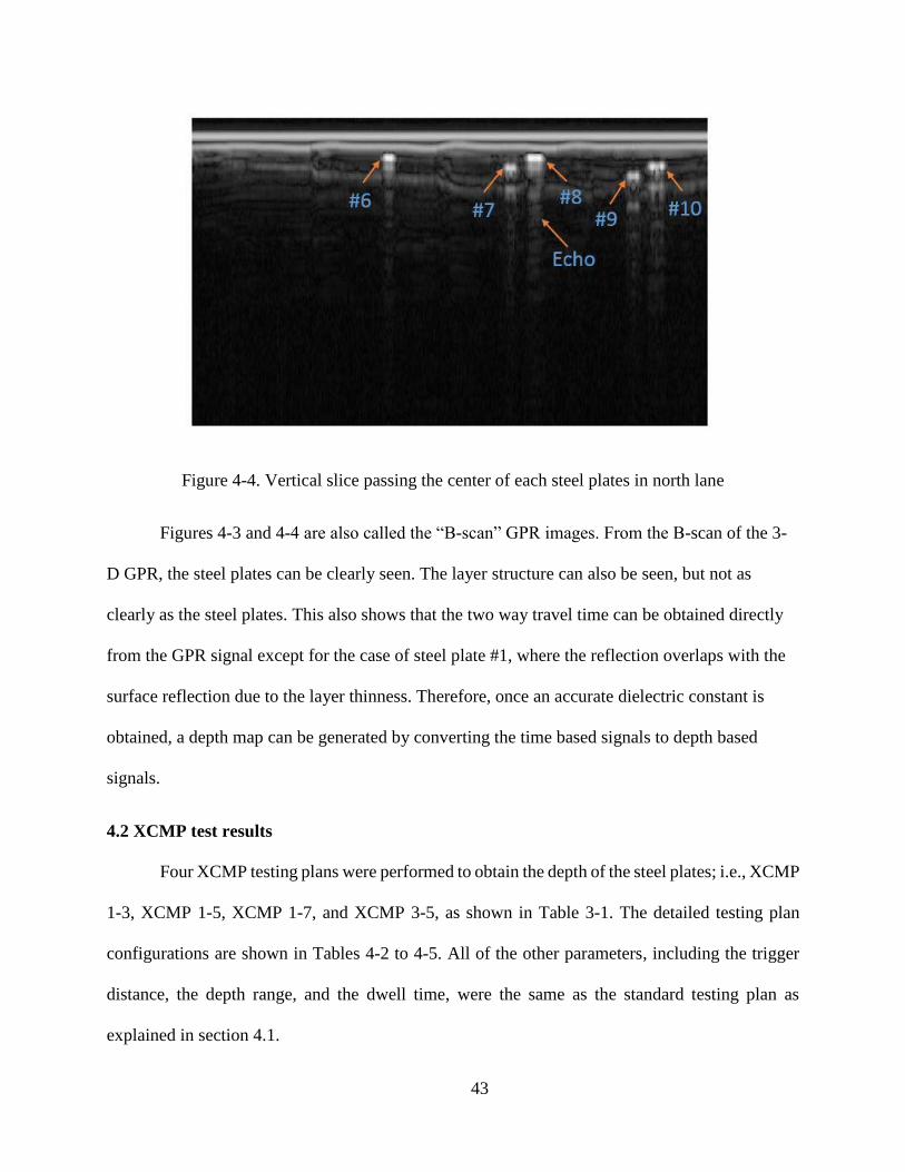
Figure 4-4. Vertical slice passing the center of each steel plates in north lane
Figures 4-3 and 4-4 are also called the “B-scan” GPR images. From the B-scan of the 3-
D GPR, the steel plates can be clearly seen. The layer structure can also be seen, but not as
clearly as the steel plates. This also shows that the two way travel time can be obtained directly
from the GPR signal except for the case of steel plate #1, where the reflection overlaps with the
surface reflection due to the layer thinness. Therefore, once an accurate dielectric constant is
obtained, a depth map can be generated by converting the time based signals to depth based
signals.
4.2 XCMP test results
Four XCMP testing plans were performed to obtain the depth of the steel plates; i.e., XCMP
1-3, XCMP 1-5, XCMP 1-7, and XCMP 3-5, as shown in Table 3-1. The detailed testing plan
configurations are shown in Tables 4-2 to 4-5. All of the other parameters, including the trigger
distance, the depth range, and the dwell time, were the same as the standard testing plan as
explained in section 4.1.
Page 50
44
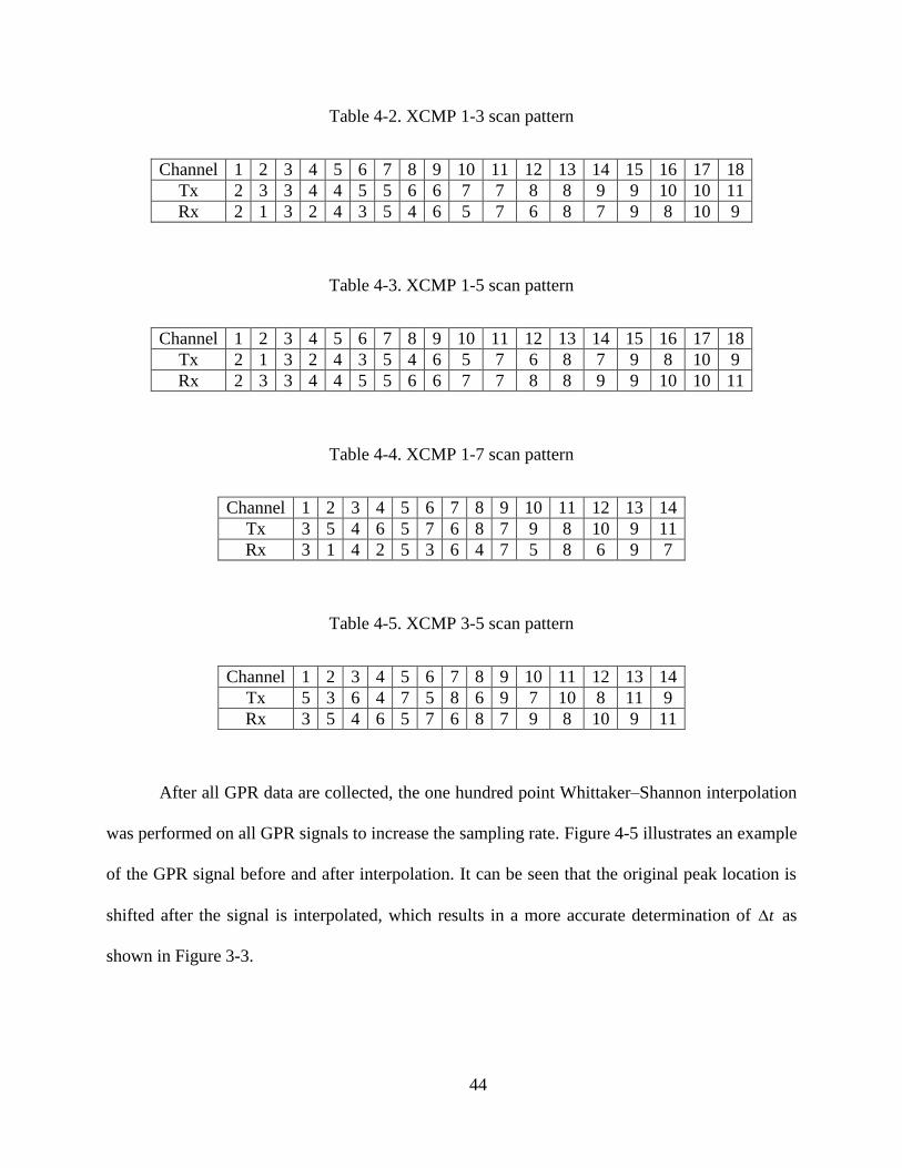
Table 4-2. XCMP 1-3 scan pattern
Channel 1 2 3 4 5 6 7 8 9 10 11 12 13 14 15 16 17 18
Tx 2 3 3 4 4 5 5 6 6 7 7 8 8 9 9 10 10 11
Rx 2 1 3 2 4 3 5 4 6 5 7 6 8 7 9 8 10 9
Table 4-3. XCMP 1-5 scan pattern
Channel 1 2 3 4 5 6 7 8 9 10 11 12 13 14 15 16 17 18
Tx 2 1 3 2 4 3 5 4 6 5 7 6 8 7 9 8 10 9
Rx 2 3 3 4 4 5 5 6 6 7 7 8 8 9 9 10 10 11
Table 4-4. XCMP 1-7 scan pattern
Channel 1 2 3 4 5 6 7 8 9 10 11 12 13 14
Tx 3 5 4 6 5 7 6 8 7 9 8 10 9 11
Rx 3 1 4 2 5 3 6 4 7 5 8 6 9 7
Table 4-5. XCMP 3-5 scan pattern
Channel 1 2 3 4 5 6 7 8 9 10 11 12 13 14
Tx 5 3 6 4 7 5 8 6 9 7 10 8 11 9
Rx 3 5 4 6 5 7 6 8 7 9 8 10 9 11
After all GPR data are collected, the one hundred point Whittaker–Shannon interpolation
was performed on all GPR signals to increase the sampling rate. Figure 4-5 illustrates an example
of the GPR signal before and after interpolation. It can be seen that the original peak location is
shifted after the signal is interpolated, which results in a more accurate determination of t as
shown in Figure 3-3.
Page 51
45
Figure 4-5. Demonstration of 100-point Whittaker–Shannon interpolation on GPR signal
The results of dielectric constants and layer thicknesses from all ten steel plates are shown
in Tables 4-6 to 4-9 for all four XCMP test configurations.
Table 4-6. Results for XCMP 1-3 configuration
Steel
Plate No. 1 2 3 4 5 6 7 8 9 10
1t (ns) 0.71 1.95 3.05 1.10 3.92 1.09 2.03 1.04 2.90 1.93
2t (ns) 0.66 1.97 3.05 1.10 3.91 1.11 2.02 1.03 2.88 1.93
1x (m) - - 0.060 - 0.083 - 0.043 - 0.091 0.043
2x (m) - - 0.065 - 0.091 - 0.047 - 0.099 0.047
1t (ns) - - 3.15 - 4.05 - 2.10 - 3.04 2.00
2t (ns) - - 3.16 - 4.06 - 2.11 - 3.05 2.01
Dielectric
Constant - - 7.36 - 6.45 - 6.98 - 4.36 6.66
Thickness
(mm) - - 172 - 236 - 117 - 214 114
Page 52
46
Table 4-7. Results for XCMP 1-5 configuration
Steel
Plate No. 1 2 3 4 5 6 7 8 9 10
1t (ns) 0.72 1.91 3.05 0.93 3.94 1.07 2.07 1.03 2.88 1.95
2t (ns) 0.66 1.89 3.03 0.91 3.91 1.05 2.05 1.02 2.86 1.94
1x (m) - 0.041 0.062 - 0.062 - 0.044 - 0.059 0.044
2x (m) - 0.051 0.076 - 0.076 - 0.054 - 0.073 0.054
1t (ns) - 1.98 3.15 - 4.04 - 2.14 - 2.98 2.03
2t (ns) - 1.99 3.18 - 4.06 - 2.16 - 3.00 2.04
Dielectric
Constant - 6.88 7.03 - 9.00 - 6.92 - 7.01 6.54
Thickness
(mm) - 111 176 - 200 - 120 - 166 117
Table 4-8. Results for XCMP 1-7 configuration
Steel
Plate No. 1 2 3 4 5 6 7 8 9 10
1t (ns) 0.69 1.95 3.04 0.98 3.89 1.11 2.09 1.04 2.88 1.96
2t (ns) 0.73 1.92 2.99 0.92 3.83 1.24 2.02 1.05 2.84 1.93
1x (m) - 0.040 0.065 - 0.074 - 0.047 - 0.068 0.038
2x (m) - 0.055 0.090 - 0.104 - 0.063 - 0.095 0.052
1t (ns) - 2.01 3.15 - 4.01 - 2.17 - 3.00 2.02
2t (ns) - 2.04 3.19 - 4.06 - 2.16 - 3.04 2.05
Dielectric Constant
- 7.27 6.68 - 7.27 - 6.61 - 6.03 7.65
Thickness (mm)
- 110 180 - 220 - 124 - 180 108
Page 53
47
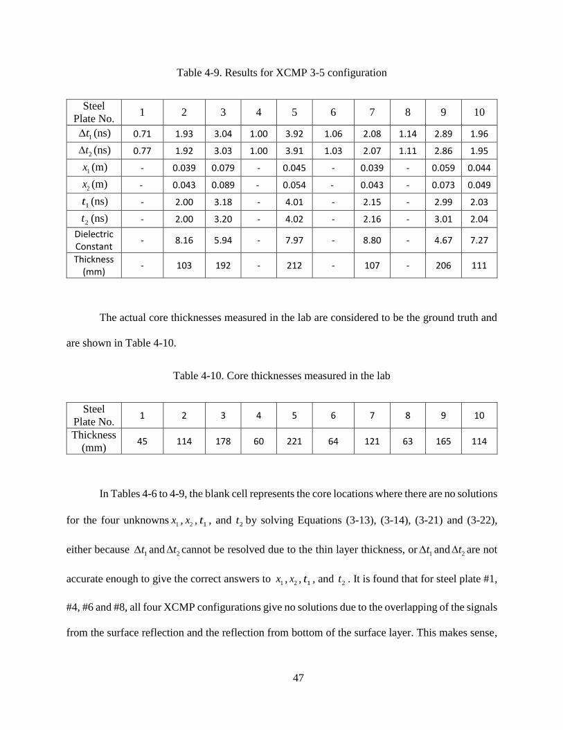
Table 4-9. Results for XCMP 3-5 configuration
Steel
Plate No. 1 2 3 4 5 6 7 8 9 10
1t (ns) 0.71 1.93 3.04 1.00 3.92 1.06 2.08 1.14 2.89 1.96
2t (ns) 0.77 1.92 3.03 1.00 3.91 1.03 2.07 1.11 2.86 1.95
1x (m) - 0.039 0.079 - 0.045 - 0.039 - 0.059 0.044
2x (m) - 0.043 0.089 - 0.054 - 0.043 - 0.073 0.049
1t (ns) - 2.00 3.18 - 4.01 - 2.15 - 2.99 2.03
2t (ns) - 2.00 3.20 - 4.02 - 2.16 - 3.01 2.04
Dielectric Constant
- 8.16 5.94 - 7.97 - 8.80 - 4.67 7.27
Thickness (mm)
- 103 192 - 212 - 107 - 206 111
The actual core thicknesses measured in the lab are considered to be the ground truth and
are shown in Table 4-10.
Table 4-10. Core thicknesses measured in the lab
Steel
Plate No. 1 2 3 4 5 6 7 8 9 10
Thickness
(mm) 45 114 178 60 221 64 121 63 165 114
In Tables 4-6 to 4-9, the blank cell represents the core locations where there are no solutions
for the four unknowns 1x , 2x , 1t , and 2t by solving Equations (3-13), (3-14), (3-21) and (3-22),
either because 1t and 2t cannot be resolved due to the thin layer thickness, or 1t and 2t are not
accurate enough to give the correct answers to 1x , 2x , 1t , and 2t . It is found that for steel plate #1,
#4, #6 and #8, all four XCMP configurations give no solutions due to the overlapping of the signals
from the surface reflection and the reflection from bottom of the surface layer. This makes sense,
Page 54
48
since steel plates #1, #4, #6 and #8 have the thinnest layers; i.e. one lift, or less than 50mm (design
thickness) according to Table 4-10. If we assume the average dielectric constant of the asphalt
pavement is 7.0, based on the analysis of the 3-D radar signals in Section 3.3.1, the Rayleigh
resolution of the EM signal is around 0.61ns, which makes the smallest possible layer thickness
that can be resolved 80.61 3 10 / 7 69.1ns m s mm . For the XCMP method, the resolution
limit is slightly different than 69.1mm depending on the EM wave incident angle.
It can also be noted that in addition to steel plates #1, #4, #6 and #8, the XCMP 1-3
configuration doesn’t have a solution for steel plate #2 either. This is because the difference
between 1t and 2t is too small: 0.02ns in this case. The value of it not only dependent on the
layer thickness, but also on the offset between the Tx and the Rx. Specifically, for the same layer
thickness, the smaller the offset between Tx and Rx, the smaller the value of it . In order to obtain
an accurate solution, we want the difference of 1t and 2t to be as large as possible. Table 4-8
shows that the difference between 1t and 2t is 0.03ns for the XCMP1-7 configuration, which is
50% larger than that of the XCMP1-3 configuration. Theoretically, the performance of the XCMP
1-7 configuration should be better than that of the XCMP 1-5 configuration, and the performance
of the XCMP 1-5 configuration should be better than that of the XCMP 1-3 and XCMP 3-5
configurations. This is also the reason why the XCMP 1-3 configuration doesn’t have a solution
for steel plate #2, although the layer thickness at steel plate #2 is larger than the resolution limit.
In practice, we should use the XCMP configuration with the largest difference between the
offset of Tx1/Rx1 and Tx2/Rx2. For example, in the case of the DX1821 antenna array (Figure 3-
6), the best XCMP configuration would be XCMP1-21, which uses Tx6/Rx6 as the first antenna
Page 55
49
pair, and Tx11/Rx1 as the second antenna pair. However, if multiple line scans are needed, the
Tx/Rx offset needs to be less than 21.
Table 4-11 shows the comparison of the prediction error of the results from all four XCMP
configurations. To visualize the different performances of the four XCMP configurations, the
prediction errors in Table 4-11 are shown in the column chart in Figure 4-6.
Table 4-11. Thickness prediction error (%) from all four XCMP configurations
Steel Plate No.
1 2 3 4 5 6 7 8 9 10 Avg.
XCMP1-3 - - 3.69 - 6.79 - 2.76 - 29.26 0.40 8.58
XCMP1-5 - 2.40 1.44 - 9.56 - 0.36 - 0.52 2.38 2.85
XCMP1-7 - 3.21 0.75 - 0.45 - 2.95 - 8.74 5.41 3.45
XCMP3-5 - 9.55 7.60 - 4.10 - 11.32 - 24.34 2.62 8.56
Avg. - 5.05 3.37 - 5.22 - 4.35 - 15.72 2.70 5.86
Figure 4-6. Relative thickness prediction errors for all four XCMP configurations
Page 56
50
From the results of all XCMP configurations for all ten steel plate locations as shown in
Table 4-11 and Figure 4-6, we can first see that the there are no solutions for steel plates #1, #4,
#6, and #8. As explained in the previous section, this is because the layer thickness is less than the
resolution limit. According to Leng (2011), the 2GHz pulsed radar manufactured by GSSI can
provide solutions to all ten steel plate locations, which implies that the time domain resolution of
the 2GHz pulsed GPR is better than that of the DX1821 3-D GPR. This was also verified in Section
3.3.1, in which it was shown that the Rayleigh resolution for 2GHz pulsed GPR is 0.54ns, while
the Rayleigh resolution for stepped frequency 3-D GPR is only 0.61ns. This observation implies
that the bandwidth, which determines the time domain resolution, of the 3-D GPR is not better
than that of the 2GHz pulsed GPR, which was expected based on the property of the stepped
frequency signal. Therefore, when no super resolution techniques are used, for thin asphalt
pavement layers the 2GHz pulsed radar will give a better result. Nonetheless, 3-D GPR has better
data collecting speed and survey area coverage, which is extremely important when large areas
need to be surveyed; e.g., an airport runway/taxiway. Hence, such information will help to select
the best approach for the given conditions.
Sufficient difference between 1t and 2t are required to solve the XCMP equations. The
difference between 1t and 2t may be increased by either increasing pavement layer thickness or
by increasing the difference between the offsets of the antenna pairs. XCMP1-3 has an insufficient
difference between 1t and 2t at steel plate #2 due to combining effect of the small difference
between Tx1/Rx1 and Tx2/Rx2. Hence, no solution could be determined.
For steel plates #2, #3, #5, #7, #9, and #10, the average relative thickness prediction errors
are 5.05%, 3.37%, 5.22%, 4.35%, 15.72%, and 2.70%, respectively. Excluding steel plate #9, the
Page 57
51
maximum average prediction error is 5.22%, which gives an absolute error of 15mm. This value
is above the construction tolerance (usually 5mm in the State of Illinois); therefore, not all XCMP
configurations are suitable for estimating asphalt pavement thickness for the purposes of QC/QA.
The cause of the high prediction error at steel plate #9 is the echoing of the surface reflection
(similar to the echoing shown in Figure 4-4), which shifts the second peak of the reflection at the
bottom of the surface layer. The echoes could be EM waves bouncing back and forth between the
layer interfaces, or between the ground surface and the 3-D GPR antenna structure. This maybe
another drawback of the 3-D GPR, since no echoing effects were found in the previous XCMP
studies (Leng 2011).
Due to the reasons explained above, XCMP1-5 and XCMP1-7 should be preferred to
XCMP1-3 and XCMP3-5. According the Table 4-11, it is confirmed that XCMP1-5 and XCMP1-
7 have average relative prediction errors of 2.85% and 3.45%, which are much better than the
accuracy of XCMP1-3 and XCMP3-5 (8.58% and 8.56%, respectively). The average absolute error
for both XCMP1-5 and XCMP1-7 configurations is 5mm, which meets the construction tolerance.
It should be noted that XCMP can be used to obtain the dielectric constant of asphalt
concrete. Specifically, if the dielectric constant is constant throughout the pavement, average
dielectric constant values may be obtained from various locations. The averaging process will
eliminate random errors such as those due to the echoing effect. Using averaged dielectric constant
and traditional two-way travel time method, an accurate thickness profile may be obtained. In this
case, the nondestructive XCMP method serves the same purpose as the dielectric constant
calibration by taking cores. The XCMP also provides greater area coverage.
Page 58
52
4.3 Summary
To measure the asphalt pavement thickness using GPR, the CMP method is preferred to
the traditional two-way travel time method, as it can be used without calibrating the dielectric
constant. XCMP method is an extended CMP method that can use two air-coupled antenna pairs
to conduct the study without using additional ground-coupled antenna pairs. The advantage of
using air-coupled antennas is that they allow to collect GPR data at highway speeds, making it
possible to survey a large area. In this study, a DX 1821 3-D GPR was used to conduct the XCMP
method.
A test site was built with various thicknesses (ranging from one lift to four lifts), and ten
steel plates are embedded under each of the asphalt lifts. A standard test pattern along with 4
XCMP configurations—XCMP1-3, XCMP1-5, XCMP1-7, and XCMP3-5—are designed to
evaluate the performance of different XCMP configurations.
From the collected data of the standard test pattern, we found that by selecting horizontal
slices at different depths, the steel plates embedded under each lift can be clearly detected. The
echoing effects can be seen from the longitudinal vertical slices. By integrating all the data
collected from 3-D GPR, a 3-D map can be generated.
For the XCMP method, the data reflected from each of the steel plates are used due to the
large reflection from the steel plates. Whittaker-Shannon interpolation was performed on the GPR
signals to increase the time domain sampling rate. The XCMP equations are numerically solved
using least squares. Cores were taken at each of the steel plates’ locations to obtain the true layer
thickness as ground truth. From the data of the four XCMP configurations, it could be concluded
that the time domain resolution of the 3-D GPR is not enough for layers thinner than 50mm.
Another valuable point is that XCMP1-5 and XCMO1-7 performs better than XCMP1-3 and
Page 59
53
XCMP3-5. Overall, the average thickness prediction error for layers thicker than 50mm is 5mm,
which is within the construction tolerance.
Page 60
54
CHAPTER 5: FINDINGS, CONCLUSIONS, AND RECOMMENDATIONS
5.1 Summary
Layer thickness is one of the most important parts of asphalt concrete pavement and one
of the most important parameters in pavement design, since it largely determines the pavement
load capacity. Layer thickness also plays a critical role in the pavement rehabilitation strategy. For
existing pavement, it is an important factor that predicts the condition of the pavement and its
remaining service life. For newly built flexible pavement, the layer thickness is used for QC/QA.
Coring has been predominantly used by agencies to obtain the asphalt layer thickness. However,
it is destructive and can only provide data at limited locations. The use of GPR to estimate the
asphalt pavement layer thickness has been studied for many years and has become the most
prevalent application of GPR in civil engineering. The major difficulty in the application is the
inaccuracy of determining the dielectric constant and the requirement of dielectric constant
calibration by taking cores. The XCMP method is an alternative to the traditional two-way travel
time method, and it can provide more accurate dielectric constant values without calibration. This
study attempts to integrate the XCMP method with a stepped-frequency antenna array—3-D
GPR—by developing signal processing techniques and numerical analysis methods.
A full-scale asphalt concrete test lane was utilized to evaluate the performance of the
XCMP method with 3-D GPR. The thickness of the asphalt pavement ranged from one lift to four
lifts (each lift is around 50.8mm thick). Steel plates were embedded under 10 locations with
different layer thicknesses to increase the reflection amplitude. Five 3-D GPR configurations were
designed: one standard scan patter, XCMP1-3, XCMP1-5, XCMP1-7, and XCMP3-5. A
Whittaker-Shannon interpolation algorithm was developed to increase the time domain sampling
Page 61
55
rate, which is important to solving the XCMP equations. A numerical solving technique based on
least square principle was introduced to solve the XCMP equations.
The introduced algorithm was used on the GPR signal reflected from ten steel plates. Cores
were taken at each of the steel plate locations and their lab-measured thicknesses were chosen as
the ground truth. A comparison of the XCMP measured thickness with the ground truth shows that
3-D GPR can be used together with the XCMP method to estimate asphalt layer thickness with
good data acquisition speed and large coverage area.
5.2 Findings
The findings of this study are summarized as following:
The time domain sampling interval of the 3-D GPR is 0.12207 ns, which is smaller
than that of the 2GHz pulsed antenna. Since the accurate determination of it is
essential for the XCMP algorithm, the Whittaker-Shannon interpolation can be
used to increase the time domain sampling rate. The interpolated signal was used
in the XCMP method and reasonable results were obtained.
The four XCMP equations can be solved numerically utilizing the least square error
approach. Constraints need to be set based on the physical representation of the
variables to ensure robustness of the outcome.
The Rayleigh resolution of stepped-frequency DX1821 3-D GPR is 0.62ns, which
is smaller than that of the 2GHz pulsed GPR. For asphalt pavement thinner than
50mm, the time domain resolution of the 3-D GPR is inadequate. Accordingly, the
bandwidth of the stepped-frequency DX1821 3-D GPR is smaller than that of the
2GHz pulsed GPR.
Page 62
56
The echo presence of the surface reflection can be overlapped with the reflection
from the bottom of the surface layer, resulting in inaccurate XCMP results.
As the difference between 1t and 2t in the XCMP is larger, the higher the
accuracy.
The average thickness estimation error for both XCMP1-5 and XCMP1-7 is 5mm,
which meets the construction tolerance. Therefore, in practice, XCMP1-5 and
XCMP1-7 are suitable for QA/QC of asphalt pavement thicker than 50mm.
5.3 Conclusions
Based on the results of the study, the following conclusions can be drawn:
Accurate determination of 1t and 2t are critical in the XCMP method. Whittaker-
Shannon interpolation can be applied to the 3-D GPR signals to increase the time
domain sampling rate.
XCMP algorithms with large difference between the offsets of the two antenna
pairs be can be used to estimate the thickness of asphalt layers which are thicker
than 50mm without calibration of dielectric constant. The average thickness
estimation error is 5mm, which is within construction tolerance.The data collection
speed of DX1821 3-D GPR is 21 times faster than that of the typical horn antenna.
Therefore, 3-D GPR may be used in large survey areas such as airport
runways/taxiways to generate a two-dimensional thickness profile or to identify
possible pavement flaws.
Page 63
57
5.4 Recommendations
This study shows the feasibility of 3-D GPR to estimate asphalt pavement thickness using
the XCMP method. As a continuation of the study, the recommendations for future study are as
follows:
For asphalt pavement thinner than 50mm, the current 3-D GPR system doesn't have
enough time domain resolution. Therefore super-resolution techniques are needed
to estimate thin layer thickness.
Effect of asphalt surface moisture on 3-D GPR signal needs to be investigated.
Since echoing effect affects the accurate determination of 1t and 2t , it is
necessary to introduce signal processing techniques to eliminate the effect of
surface reflection echoes.
The performance of other 3-D GPR models should be studied.
Page 64
58
References
3D-Radar GPR. 2015. http://www.3d-radar.com/.
Al-Qadi, I. L., Ghodgaonkar D., Varada V., and Varadan V., 1991. “Effect of Moisture on
Asphaltic Concrete at Microwave Frequencies.” IEEE Transactions on Geoscience and
Remote Sensing, 29.5, 710-717.
Al-Qadi, I., Lahouar S., and Loulizi A., 2001. “In Situ Measurements of Hot-Mix Asphalt
Dielectric Properties.” NDT & E International, 34.6, 427-434.
Al-Qadi, I., Lahouar S., and Loulizi. A., 2003. “Successful Application of Ground-Penetrating
Radar for Quality Assurance-Quality Control of New Pavements.” Transportation
Research Record: Journal of the Transportation Research Board, 1861.1, 86-97.
Al-Qadi, I., and Lahouar S., 2005. “Measuring Layer Thicknesses with GPR–Theory to Practice.”
Construction and Building Materials, 19.10, 763-772.
Al-Qadi, I.L., Leng Z., Lahouar S., Baek J., 2010. “In-place hot-mix asphalt density estimation
using ground-penetrating radar.” Transportation Research Record: Journal of the
Transportation Research Board, 2152.1, 19-27.
ASTM D6432 - 11. “Standard Guide for using the Surface Ground Penetrating Radar Method for
Subsurface Investigation.”
Blahut, Richard E., 2004. Theory of remote image formation. Cambridge University Press.
Claessen, A. I. M., Edwards J. M., Sommer P., and Uge P., 1977. “Asphalt Pavement Design--The
Shell Method.” In Volume I of proceedings of 4th International Conference on Structural
Design of Asphalt Pavements, Ann Arbor, Michigan, August 22-26, 1977 (No. Proceeding).
Culick, F. E. C., 1987. “A note on Rayleigh's criterion.” Combustion Science and Technology, 56.
4-6, 159-166.
Chang, C. W., Lin C. H., and Lien H. S., 2009. “Measurement Radius of Reinforcing Steel Bar in
5 Concrete using Digital Image GPR.” Construction and Building Materials, 23.2, 1057-
1063.
Chuang, S. L., 2012. Physics of photonic devices. 80. John Wiley & Sons.
Daniels, David J., 2005. Ground penetrating radar. John Wiley & Sons, Inc.
Eide, Egil S., 2000. “Ultra-wideband transmit/receive antenna pair for ground penetrating radar.”
IEE Proceedings-Microwaves, Antennas and Propagation, 147.3, 231-235.
Eide, E. S., and Jens F. H., 2002. “3D utility mapping using electronically scanned antenna array.”
Ninth International Conference on Ground Penetrating Radar (GPR2002), International
Society for Optics and Photonics.
Eide, E., and Sala J., 2012. High Resolution Step-Frequency 3D GPR Using Wideband Antenna
Arrays (Presentation at Seminar of Ground Penetrating Radar in Road Monitoring and
Evaluation Now and the Future).
Page 65
59
Huang, Y. H., 1993. Pavement analysis and design. Transportation Research Board.
Huisman, J., Sperl C., Bouten W., and Verstraten J., 2001. “Soil Water Content Measurements at
Different Scales: Accuracy of Time Domain Reflectometry and Ground-Penetrating Radar.”
Journal of Hydrology, 245.1, 48-58.
IEEE Standard 145-1993, 1993. IEEE Standard Definitions of Terms for Antennas.
Jin, Jian-Ming., 2011. Theory and computation of electromagnetic fields. John Wiley & Sons.
Jol, Harry M., ed., 2008. Ground penetrating radar theory and applications. Elsevier.
Kassem, E., Scullion T., Masad E., and Chowdhury A., 2012. “Comprehensive Evaluation of
Compaction of Asphalt Pavements and a Practical Approach for Density Predictions.”
Transportation Research Record: Journal of the Transportation Research Board, 2268.1,
98–107.
Lahouar, S., Al-Qadi I., Loulizi A., Clark T., and Lee D., 2002. “Approach to Determining in Situ
Dielectric Constant of Pavements: Development and Implementation at Interstate 81 in
Virginia.” Transportation Research Record: Journal of the Transportation Research
Board. 1806.1, 81-87.
Lahouar, S., 2003. “Development of data analysis algorithms for interpretation of ground
penetrating radar data (Doctoral dissertation, Virginia Polytechnic Institute and State
University).”
Le Bastard, C., Baltazart V., Derobert X., and Wang Y., 2012. “Support Vector Regression method
applied to thin pavement thickness estimation by GPR.” Ground Penetrating Radar (GPR),
2012 14th International Conference on IEEE, 349-353.
Leckebusch, J., 2011. “Comparison of a stepped‐frequency continuous wave and a pulsed GPR
system.” Archaeological Prospection, 18.1, 15-25.
Leng, Z., Al-Qadi I.L., Lahouar S., 2011. “Development and validation for in situ asphalt mixture
density prediction models.” NDT & E International, 44, 369-375.
Leng, Z., 2011. “Prediction of in-situ asphalt mixture density using ground penetrating radar:
theoretical development and field verification (Doctoral dissertation, University of Illinois
at Urbana-Champaign).”
Leng, Z., Al-Qadi, I. L., Shangguan P., Son S., 2012. “Field application of ground penetrating
radar for asphalt mixture density measurement: a case study of Illinois Route 72 Overlay.”
Transportation Research Record: Journal of the Transportation Research Board, 2304,
133–141.
Leng, Z., and Al-Qadi I. L., 2014. “An innovative method for measuring pavement dielectric
constant using the extended CMP method with two air-coupled GPR systems.” NDT & E
International, 66, 90-98.
Liu, H., Takahashi K., and Sato M., 2014. “Measurement of Dielectric Permittivity and Thickness
of Snow and Ice on a Brackish Lagoon using GPR.” IEEE Journal of Selected Topics in
Applied Earth Observations and Remote Sensing, 7.3, 820-827.
Page 66
60
Liu, H., and Sato M., 2014. “In Situ Measurement of Pavement Thickness and Dielectric
Permittivity by GPR using an Antenna Array.” NDT & E International, 64, 65-71.
Lyons, Richard G., 2010. Understanding digital signal processing. Pearson Education.
Masad, E., Al-Rub R. A., and Little D. N., 2012. “Recent Developments and Applications of
Pavement Analysis Using Nonlinear Damage (PANDA) Model.” In 7th RILEM
International Conference on Cracking in Pavements (pp. 399-408). Springer Netherlands.
Morey, R. M., 1998. Ground Penetrating Radar for Evaluating Subsurface Conditions for
Transportation Facilities. Transportation Research Board.
Roberts, F. L., Kandhal P. S., Brown E. R., Lee D.Y., and Kennedy T. W., 1996. “Hot mix asphalt
materials, mixture design and construction.”
Saarenketo, T., 1997. "Using ground-penetrating radar and dielectric probe measurements in
pavement density quality control." Transportation Research Record: Journal of the
Transportation Research Board, 1575.1, 34-41.
Saarenketo, T., and Scullion T., 2000. “Road Evaluation with Ground Penetrating Radar.” Journal
of Applied Geophysics, 43.2-4, 119–138.
Schneider, W. A., 1984. “The common depth point stack.” Proceedings of the IEEE, 72.10, 1238-
1254.
Shangguan, P., Al-Qadi I., Coenen A., and Zhao S., 2014a. “Algorithm development for the
application of ground-penetrating radar on asphalt pavement compaction monitoring.”
International Journal of Pavement Engineering, 1-12.
Shangguan, P., and Al-Qadi, I. L., 2014b. “Calibration of FDTD simulation of GPR signal for
asphalt pavement compaction monitoring.” IEEE Transactions on Geoscience and Remote
Sensing, 53.3, 1538-1548.
Shangguan, P., 2015. “Development of algorithms for asphalt pavement compaction monitoring
utilizing ground penetrating radar.” Diss. University of Illinois at Urbana-Champaign.
Stutzman, W. L., and Thiele G. A., 2012. Antenna theory and design. John Wiley & Sons.
Uda, S. 1928. “On the Wireless Beam of Short Electric Waves”. Institute of Electrical Engineers
of Japan.
Yilmaz, Ö., 2008. “Seismic data analysis: processing, inversion, and interpretation of seismic data.”
Tulsa: Society of Exploration Geophysicists.
Yoder, E. J., and Witczak M. W., 1975. Principles of pavement design. John Wiley & Sons.
Zhao, S., Shangguan P., and Al-Qadi I., 2015. “Application of Regularized Deconvolution
Technique for Predicting Pavement Thin Layer Thicknesses from Ground Penetrating
Radar Data.” NDT & E International, 73, 1-7.