Page 1
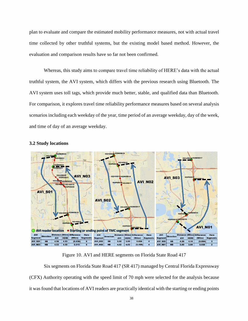
University of Central Florida University of Central Florida
STARS STARS
Electronic Theses and Dissertations
2019
Development of Decision Support System for Active Traffic Development of Decision Support System for Active Traffic
Management Systems Considering Travel Time Reliability Management Systems Considering Travel Time Reliability
Whoibin Chung University of Central Florida
Part of the Civil Engineering Commons, and the Transportation Engineering Commons
Find similar works at: https://stars.library.ucf.edu/etd
University of Central Florida Libraries http://library.ucf.edu
This Doctoral Dissertation (Open Access) is brought to you for free and open access by STARS. It has been accepted
for inclusion in Electronic Theses and Dissertations by an authorized administrator of STARS. For more information,
please contact [email protected] .
STARS Citation STARS Citation Chung, Whoibin, "Development of Decision Support System for Active Traffic Management Systems Considering Travel Time Reliability" (2019). Electronic Theses and Dissertations. 6467. https://stars.library.ucf.edu/etd/6467
Page 2
DEVELOPMENT OF DECISION SUPPORT SYSTEM FOR ACTIVE
TRAFFIC MANAGEMENT SYSTEMS CONSIDERING TRAVEL TIME
RELIABILITY
by
WHOIBIN CHUNG
B.S., Ajou University, South Korea, 1998
M.S., Ajou University, South Korea, 2000
A dissertation submitted in partial fulfillment of the requirements
for the degree of Doctor of Philosophy
in the Department of Civil, Environmental and Construction Engineering
in the College of Engineering and Computer Science
at the University of Central Florida
Orlando, Florida
Summer Term
2019
Major Professor: Mohamed Abdel-Aty
Page 3
ii
ABSTRACT
As traffic problems on roadways have been increasing, active traffic management systems
(ATM) using proactive traffic management concept have been deployed on freeways and arterials.
The ATM aims to integrate and automate various traffic control strategies such as variable speed
limits, queue warning, and ramp metering through a decision support system (DSS). Over the past
decade, there have been many efforts to integrate freeways and arterials for the efficient operation
of roadway networks. It has been required that these systems should prove their effectiveness in
terms of travel time reliability. Therefore, this study aims to develop a new concept of a decision
support system integrating variable speed limits, queue warning, and ramp metering on the basis
of travel time reliability of freeways and arterials.
Regarding the data preparation, in addition to collecting multiple data sources such as
traffic data, crash data and so on, the types of traffic data sources that can be applied for the analysis
of travel time reliability were investigated. Although there are many kinds of real-time traffic data
from third-party traffic data providers, it was confirmed that these data cannot represent true travel
time reliability through the comparative analysis of measures of travel time reliability. Related to
weather data, it was proven that nationwide land-based weather stations could be applicable.
Since travel time reliability can be measured by using long-term periods for more than six
months, it is necessary to develop models to estimate travel time reliability through real-time traffic
data and event-related data. Among various matrix to measure travel time reliability, the standard
deviation of travel time rate [minute/mile] representing travel time variability was chosen because
it can represent travel time variability of both link and network level. Several models were
Page 4
iii
developed to estimate the standard deviation of travel time rate through average travel time rate,
the number of lanes, speed limits, and the amount of rainfall.
Finally, a DSS using a model predictive control method to integrate multiple traffic control
measures was developed and evaluated. As a representative model predictive control, METANET
model was chosen, which can include variable speed limit, queue warning, and ramp metering,
separately or combined. The developed DSS identified a proper response plan by comparing travel
time reliability among multiple combinations of current and new response values of strategies. In
the end, it was found that the DSS provided the reduction of travel time and improvement of its
reliability for travelers through the recommended response plans.
Page 5
iv
ACKNOWLEDGMENTS
Foremost, I would like to express my sincere gratitude to my advisor Prof. Mohamed
Abdel-Aty for the continuous support of my Ph.D. study and research, for his patience, motivation,
enthusiasm, and immense knowledge. His guidance helped me in all the time of research and
writing of this dissertation. Besides my advisor, I would like to thank the rest of my thesis
committee: Dr. Naveen Eluru, Dr. Samiul Hasan, Dr. Qing Cai, and Dr. Hsin-Hsiung Huang.
I thank my fellow labmates: Yaobang Gong, and Mdhasibur Rahman, for the AIMSUN
stimulation in the IATM project. In particular, I am grateful to Dr. Hochul Park for helping me the
data analysis.
Last but not the least, I would like to thank my wife and daughter, for always supporting
me throughout my Ph.D. course.
Page 6
v
TABLE OF CONTENTS
LIST OF FIGURES ....................................................................................................................... xi
LIST OF TABLES ........................................................................................................................ xv
CHAPTER 1. INTRODUCTION ................................................................................................... 1
1.1 Overview ............................................................................................................................... 1
1.2 Research Objectives .............................................................................................................. 4
CHAPTER 2. LITERATURE REVIEW ........................................................................................ 6
2.1 Active Traffic Management (ATM) ..................................................................................... 6
2.2 Integrated Corridor Management (ICM) ............................................................................ 13
2.3 Decision Support Systems (DSS) ....................................................................................... 16
2.3.1 Knowledge-based DSS ................................................................................................ 17
2.3.2 DSS using real-time traffic simulation ........................................................................ 19
2.3.3 Case-based DSS without real-time traffic simulation .................................................. 23
2.3.4 Other DSS .................................................................................................................... 24
2.4 Travel Time Reliability ....................................................................................................... 26
2.4.1 Measures of travel time reliability ............................................................................... 26
2.4.2 Impact factors of travel time reliability ....................................................................... 28
2.4.3 Estimation of travel time distribution or reliability ..................................................... 30
Page 7
vi
2.5 Summary ............................................................................................................................. 32
CHAPTER 3. AVAILABILITY OF HERE DATA FOR TRAVEL TIME RELIABILITY ....... 34
3.1 Introduction ......................................................................................................................... 34
3.2 Study locations .................................................................................................................... 38
3.3 Data Preparation.................................................................................................................. 39
3.4 Analysis Scenarios .............................................................................................................. 40
3.5 Travel Time Data Distribution of AVI and HERE ............................................................. 41
3.6 Analysis Results .................................................................................................................. 45
3.7 Conclusion .......................................................................................................................... 51
CHAPTER 4. THE EFFECTIVE COVERAGE OF LAND-BASED WEATHER STATIONS . 54
4.1 Introduction ......................................................................................................................... 54
4.2 Literature Review................................................................................................................ 56
4.3 Data Preparation.................................................................................................................. 59
4.3.1 Nationwide QCLCD .................................................................................................... 59
4.3.2 Nationwide fatal crashes .............................................................................................. 61
4.3.3 Nationwide AADT of the Highway Performance Monitoring System (HPMS) ......... 62
4.3.4 Grouping of weather types of QCLCD and FARS data .............................................. 62
4.4 Regional Characteristics of Weather and Weather-related Fatal Crashes .......................... 63
4.5 Viability of QCLCD for Traffic Safety Evaluation ............................................................ 66
Page 8
vii
4.6 Model Development to Estimate Weather-related Fatal Crashes ....................................... 72
4.7 Discussion and Conclusions ............................................................................................... 76
CHAPTER 5. METHOD FOR ESTIMATING VEHICLE-TO-VEHICLE TRAVEL TIME
VARIABILITY MODELS AT THE LINK AND NETWORK LEVELS OF
FREEWAYS/EXPRESSWAYS ................................................................................................... 80
5.1 Introduction ......................................................................................................................... 81
5.2 Study Area .......................................................................................................................... 84
5.3 Methodology ....................................................................................................................... 87
5.3 Data preparation .................................................................................................................. 92
5.3.1 Mean Travel Time and its SD of Links on CFX’s Expressways ................................. 93
5.3.2 Link Travel Time of I-4 and expressways of FTE ....................................................... 95
5.3.3 MVDS Data ................................................................................................................. 95
5.3.3 Crash Location and its Duration .................................................................................. 96
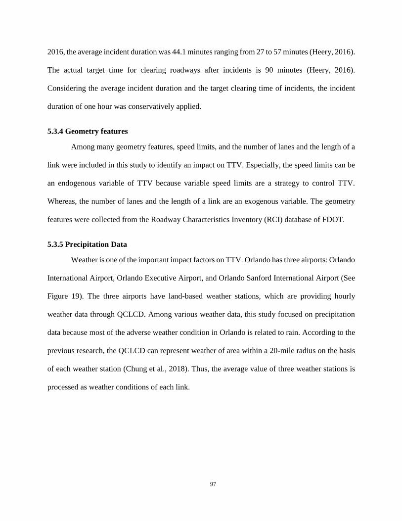
5.3.4 Geometry features ........................................................................................................ 97
5.3.5 Precipitation Data......................................................................................................... 97
5.4 TTV of freeways and expressways in the Orlando area ..................................................... 98
5.5 Modeling results and their implication ............................................................................. 103
5.6 Discussion and conclusion ................................................................................................ 108
CHAPTER 6. IDENTIFICATION OF CRITICAL ROADWAYS AND SEGMENTS ............ 112
6.1 Identification methods ...................................................................................................... 112
Page 9
viii
6.1.1 Performance measures ............................................................................................... 113
6.1.2 Performance Measure Estimation by Direction of Roadways ................................... 115
6.1.3 Normalization and combination of performance measures ....................................... 116
6.1.4 Categorization and combination of performance measures ....................................... 117
6.2 Data preparation ................................................................................................................ 119
6.3 Evaluation results .............................................................................................................. 122
6.3.1 Identification of critical roadways ............................................................................. 124
6.3.2 Identification of Critical Segments ............................................................................ 127
CHAPTER 7. DEVELOPMENT OF DECISION SUPPORT SYSTEM (dss) TO MITIGATE
TRAVEL TIME VARIABILITY THROUGH THE COMBINATION OF VARIABLE SPEED
LIMITS, QUEUE WARNING, and RAMP METERING.......................................................... 130
7.1 Introduction ....................................................................................................................... 130
7.2 Decision Support System .................................................................................................. 131
7.3 Rules of Active Traffic Management Strategies ............................................................... 132
7.3.1 VSL (Variable Speed Limits) Control Rule............................................................... 132
7.3.2 QW (Queue Warning) Control Rule .......................................................................... 134
7.3.3 RM (Ramp Metering) Control Rule ........................................................................... 137
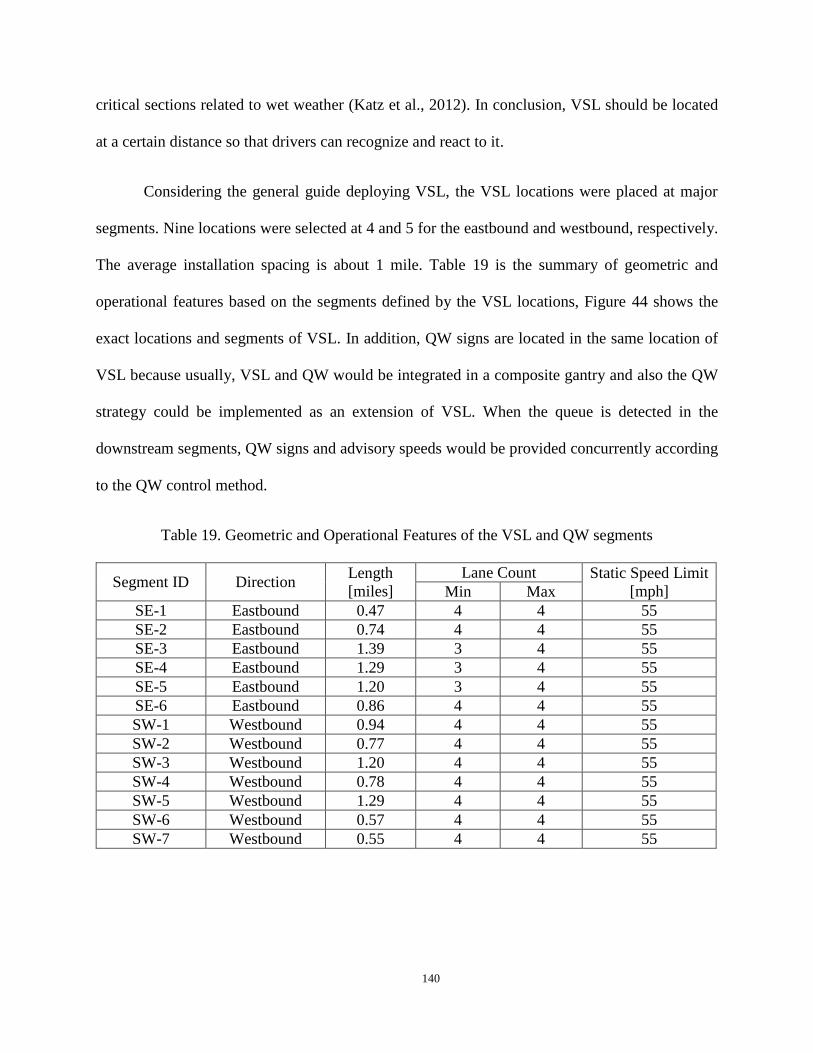
7.4 Study Site .......................................................................................................................... 138
7.4.1 Selection of VSL and QW Deployment Location ..................................................... 139
7.4.2 Selection of RM Deployment Location ..................................................................... 141
Page 10
ix
7.5 A Macroscopic Traffic Flow Model for the Freeway and Arterial Network .................... 144
7.5.1 Freeway Traffic Model .............................................................................................. 144
7.5.2 Arterial Traffic Model ................................................................................................ 146
7.6 Travel Time Reliability Model ......................................................................................... 148
7.7 AIMSUN Simulation Setup .............................................................................................. 152
7.8 Development of possible simulation scenarios related to IATM ...................................... 155
7.9 Evaluation Results of possible operational strategies of IATM ....................................... 157
7.9.1 Extreme Traffic Congestion ....................................................................................... 158
7.9.2 Heavy Traffic Congestion .......................................................................................... 159
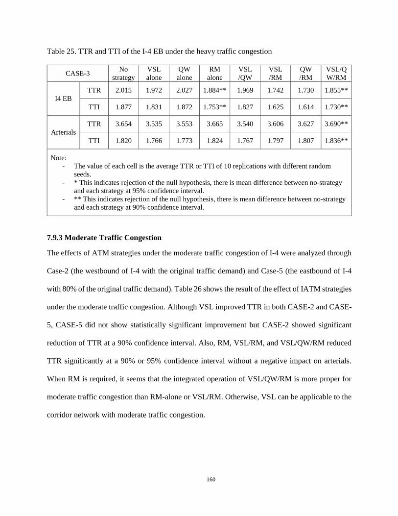
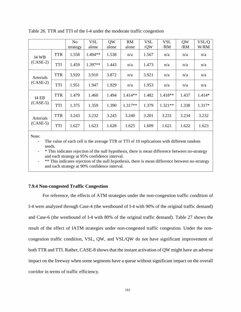
7.9.3 Moderate Traffic Congestion ..................................................................................... 160
7.9.4 Non-congested Traffic Congestion ............................................................................ 161
7.9.5 Discussion .................................................................................................................. 162
7.10 Effectiveness of Integrated ATM strategies with DSS ................................................... 164
7.10.1 Extreme Traffic Congestion ..................................................................................... 165
7.10.2 Heavy Traffic Congestion ........................................................................................ 166
7.10.3 Moderate Traffic Congestion ................................................................................... 167
7.11 Conclusions ..................................................................................................................... 169
CHAPTER 8. CONCLUSIONS ................................................................................................. 171
REFERENCES ........................................................................................................................... 173
Page 12
xi
LIST OF FIGURES
Figure 1. Continuum of operations strategies (Neudorff and McCabe, 2015) ............................... 2
Figure 2. Gantry with speed displays, lane control and supplemental signs ................................ 10
Figure 3. I-66 ATM project segments and treatments .................................................................. 11
Figure 4. Intelligent lane control signals on I-35W ...................................................................... 12
Figure 5. Active Traffic Management system on I-94 (Source: http://ungemah.com/sh_projects/i-
94-managed-lanes-study-phase-1/) ............................................................................................... 13
Figure 6. Generic view about DSS ............................................................................................... 17
Figure 7. Working process of the real-time evaluation and decision support system (Hu et al., 2003)
....................................................................................................................................................... 20
Figure 8. Framework of TrEPS-based decision support system for weather-responsive traffic
signal operations (Kim et al., 2014) .............................................................................................. 21
Figure 9. Overall structure of the intelligent traffic control decision support system (Almejalli et
al., 2007) ....................................................................................................................................... 24
Figure 10. AVI and HERE segments on Florida State Road 417 ................................................. 38
Figure 11. Scatter plots of 5-minute travel rates for all segments ................................................ 43
Figure 12. Empirical Cumulative Distributions (ECD) of average travel rate for time of day in 5-
minutes increment ......................................................................................................................... 44
Page 13
xii
Figure 13. Locations of weather stations in the USA ................................................................... 60
Figure 14. USA Climate Regions ................................................................................................. 63
Figure 15. Annual average percentages of observation duration of rain, snow, and fog (2008-2014)
....................................................................................................................................................... 64
Figure 16. Annual average fatal crash frequency under rain, snow, and fog by climate region (2007-
2014) ............................................................................................................................................. 65
Figure 17. Method of matching time and weather conditions between FARS and QCLCD........ 68
Figure 18. Regional Sensitivity and Positive Predictive Value (PPV) by weather conditions ..... 72
Figure 19. Freeways and expressways in Orlando area (CFX, 2016) .......................................... 85
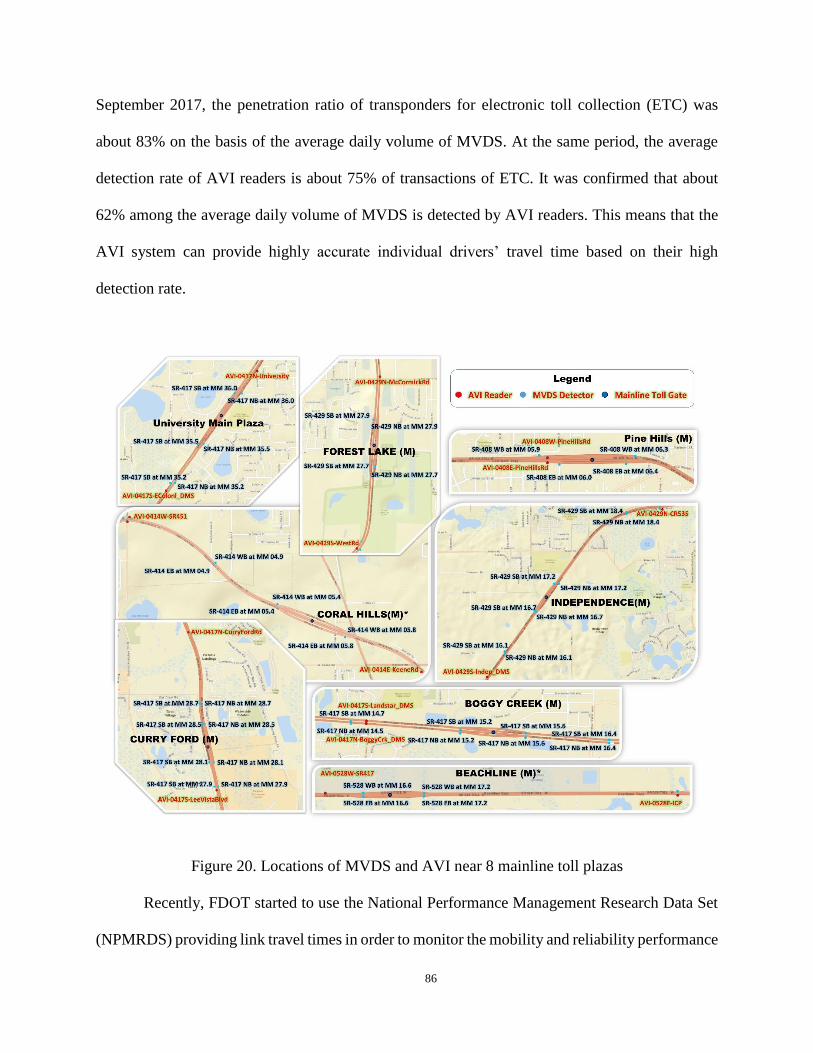
Figure 20. Locations of MVDS and AVI near 8 mainline toll plazas .......................................... 86
Figure 21. A framework estimating both vehicle-to-vehicle and day-to-day TTV ...................... 89
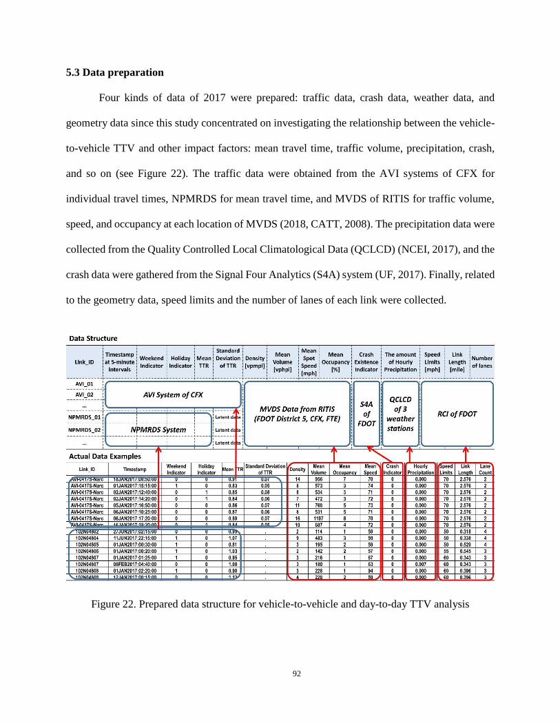
Figure 22. Prepared data structure for vehicle-to-vehicle and day-to-day TTV analysis ............. 92
Figure 23. Link travel time estimation steps from AVI raw data ................................................. 93
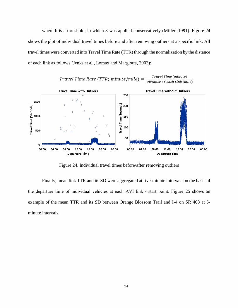
Figure 24. Individual travel times before/after removing outliers ................................................ 94
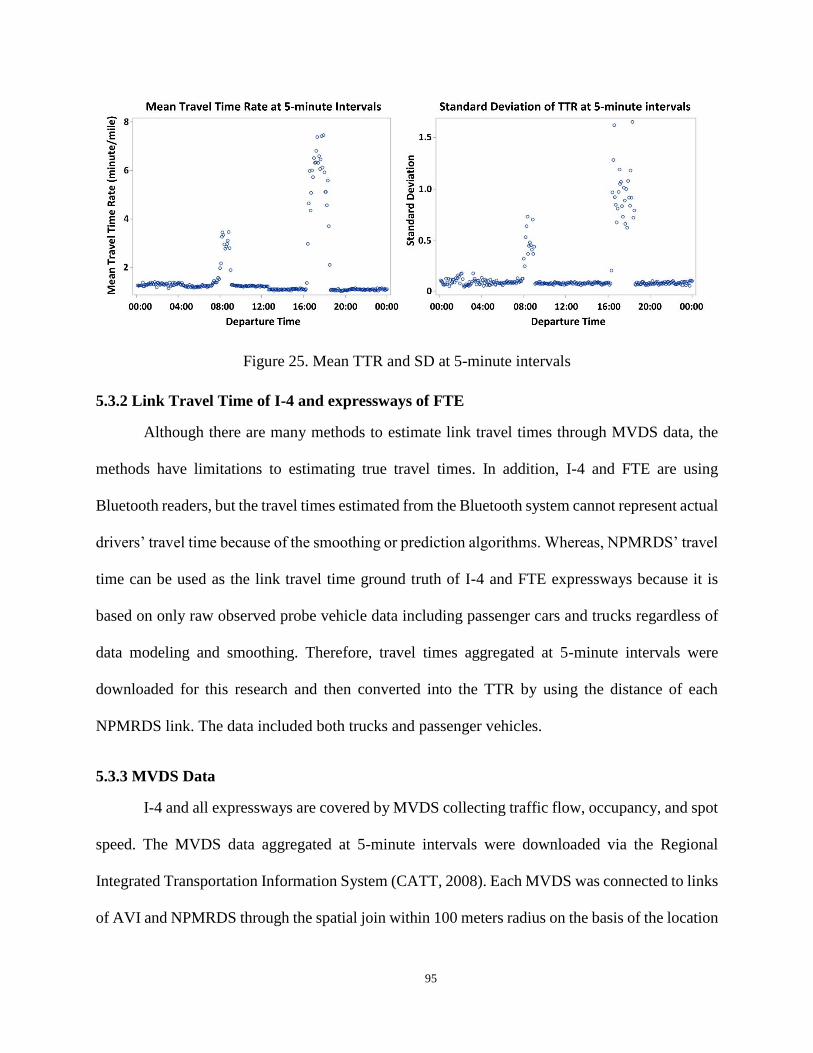
Figure 25. Mean TTR and SD at 5-minute intervals .................................................................... 95
Figure 26. Spatial Join with Links and MVDS ............................................................................. 96
Figure 27. The relationship between mean TTR and its SD representing vehicle-to-vehicle TTV at
the link and network levels ........................................................................................................... 98
Page 14
xiii
Figure 28. The relationship between mean TTR and its SD representing day-to-day TTV at the
link and network levels ............................................................................................................... 100
Figure 29. Day-to-day TTV with or without vehicle-to-vehicle TTV, or of only vehicle-to-vehicle
TTV ............................................................................................................................................. 101
Figure 30. Relationship between NFD and SD of TTR at the network level ............................. 102
Figure 31. Density versus SD of TTR and TTR ......................................................................... 105
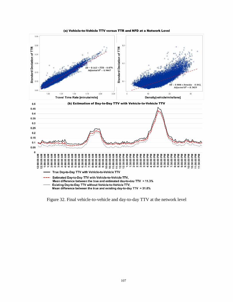
Figure 32. Final vehicle-to-vehicle and day-to-day TTV at the network level .......................... 107
Figure 33. The relationship among TTI, PTI, and BTI of 2017 ................................................. 116
Figure 34. Normalized TTI, PTI, and BTI of 2017 .................................................................... 117
Figure 35. 50th and 75th percentile of performance measures: TTI, PTI, and BTI ..................... 118
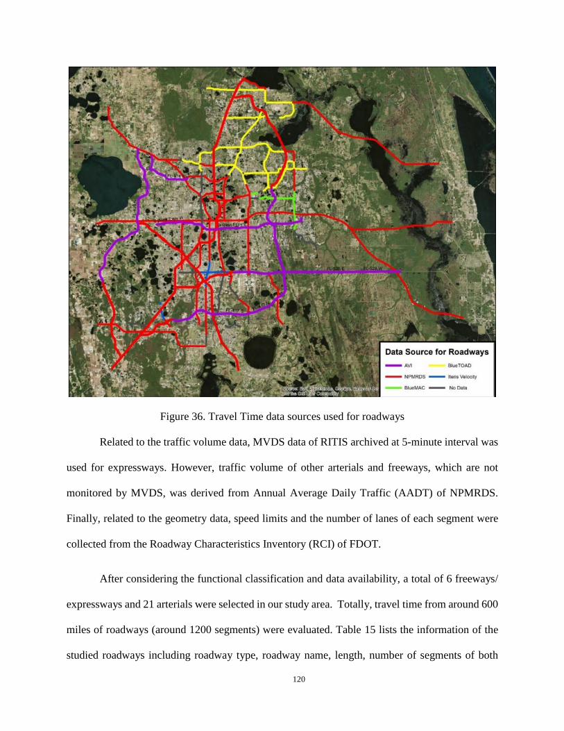
Figure 36. Travel Time data sources used for roadways ............................................................ 120
Figure 37. TTI, PTI, and BTI at the freeway/expressways network level .................................. 122
Figure 38. TTI, PTI, and BTI at the arterial network level ......................................................... 123
Figure 39. Categorization of TTI, PTI, and BTI on segments for AM and PM peak periods .... 128
Figure 40. Critical segments in Orlando area ............................................................................. 129
Figure 41. Decision Support System Configuration ................................................................... 132
Figure 42. VSL Control Logic .................................................................................................... 133
Page 15
xiv
Figure 43. An example of the gradual speed reduction of upstream segments .......................... 137
Figure 44. Study site ................................................................................................................... 139
Figure 45. The Location of Metered Ramps ............................................................................... 143
Figure 46. METANET for arterial .............................................................................................. 147
Figure 47. Microscopic simulation area in Downtown Orlando (I4, SR 408 etc.) ..................... 152
Figure 48. GEH value representation for Downtown Orlando area ........................................... 154
Figure 49. TTR and TTI at the entire network under the extreme traffic condition (I-4) .......... 166
Figure 50. Scatter plot of TTR and TTI of freeways and arterials under the extreme traffic condition
(I-4) ............................................................................................................................................. 166
Figure 51. TTR and TTI at the entire network under the heavy traffic condition (I-4) .............. 167
Figure 52. Scatter plot of TTR and TTI of freeways and arterials under the heavy traffic condition
(I-4) ............................................................................................................................................. 167
Figure 53. TTR and TTI at the entire network under the moderate traffic condition (I-4) ........ 168
Figure 54. Scatter plot of TTR and TTI of freeways and arterials under the moderate traffic
condition (I-4) ............................................................................................................................. 168
Figure 55. The suggested new conceptual DSS for active traffic management systems ............ 171
Page 16
xv
LIST OF TABLES
Table 1. Potential benefits of Active Traffic Management (Mirshahi et al., 2007) ........................ 6
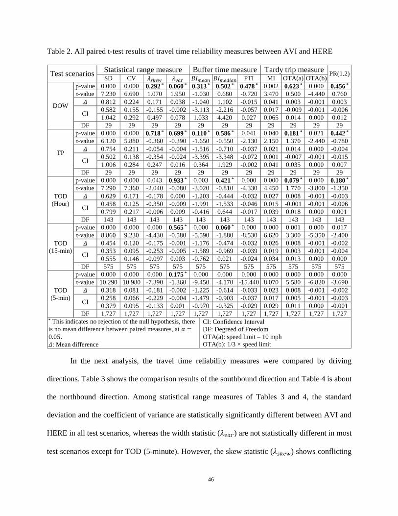
Table 2. All paired t-test results of travel time reliability measures between AVI and HERE .... 46
Table 3. Paired t-test results of travel time reliability measures between AVI and HERE of the
southbound direction ..................................................................................................................... 47
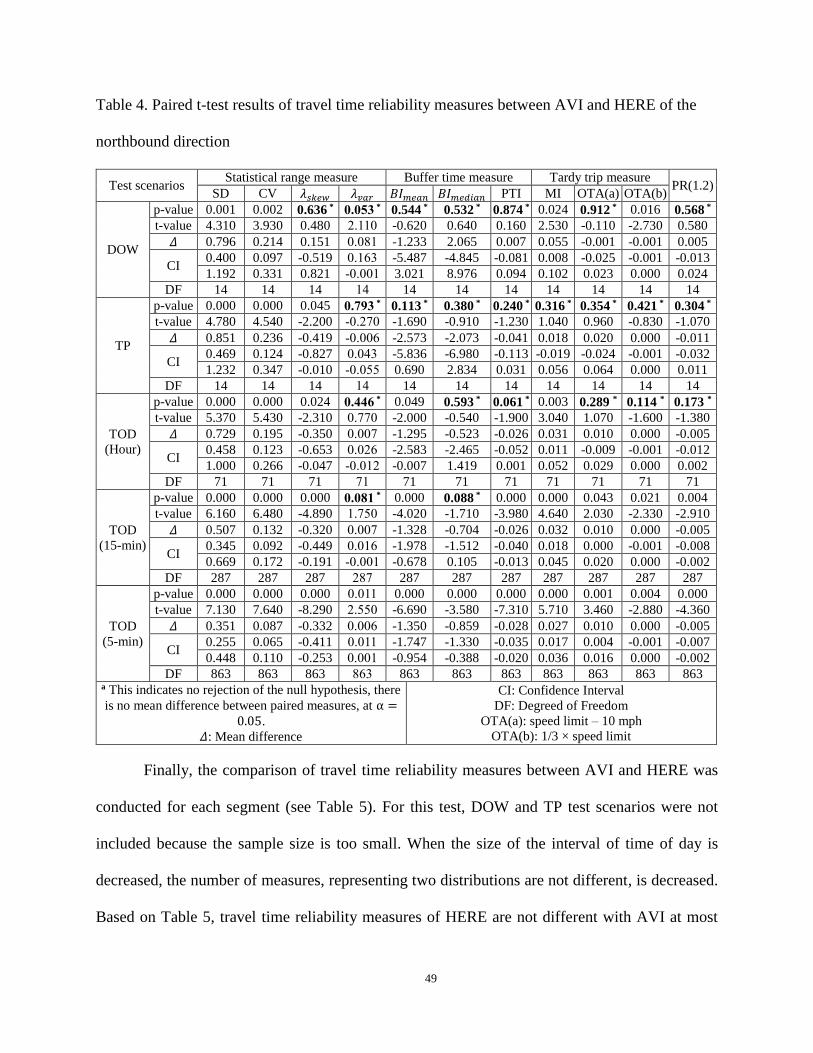
Table 4. Paired t-test results of travel time reliability measures between AVI and HERE of the
northbound direction ..................................................................................................................... 49
Table 5. Paired t-test results (p-value) of travel time reliability measures between AVI and HERE
of each segment............................................................................................................................. 50
Table 6. Weather-related fatal crashes by year (2007-2014) ........................................................ 61
Table 7. Reclassification of weather types of QCLCD and FARS data ....................................... 63
Table 8. 2×2 contingency table and statistical measurements ...................................................... 68
Table 9. Contingency tables for matching QCLCD and FARS weather data by coverage (May
2007 to Dec 2014) ......................................................................................................................... 70
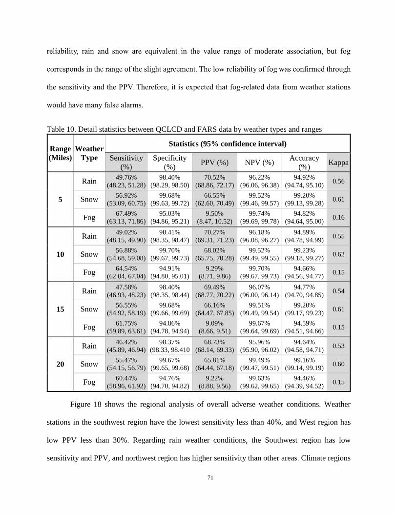
Table 10. Detail statistics between QCLCD and FARS data by weather types and ranges ......... 71
Table 11. Negative binomial model of regional annual fatal crash frequency by each weather
condition including clear and cloud .............................................................................................. 74
Page 17
xvi
Table 12. Regional relationship between total fatal crashes and duration of adverse weather type
....................................................................................................................................................... 75
Table 13. Descriptive statistics of independent variables ........................................................... 104
Table 14. Tobit model estimation results .................................................................................... 104
Table 15. List of the evaluated roadways ................................................................................... 121
Table 16. Ranking results of freeways/expressways .................................................................. 124
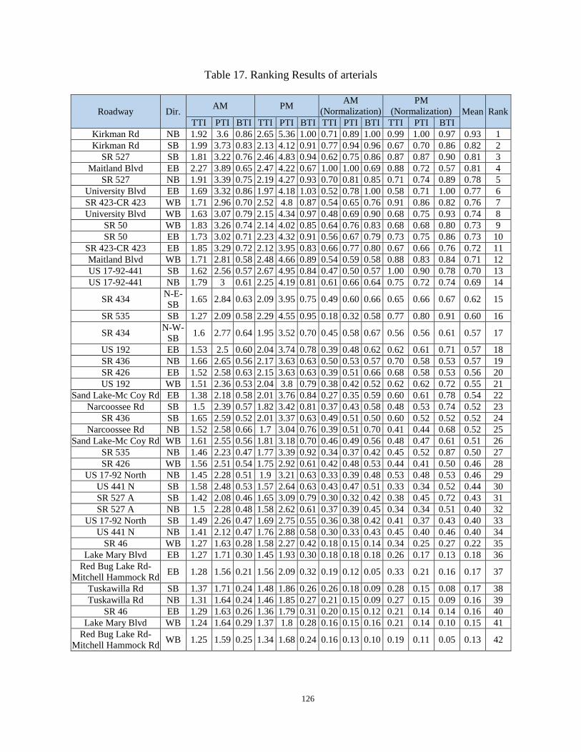
Table 17. Ranking Results of arterials ........................................................................................ 126
Table 18. Local Actuated Metering Rates as a Function of Mainline Occupancy ..................... 138
Table 19. Geometric and Operational Features of the VSL and QW segments ......................... 140
Table 20. Results of the Tobit Model to Calculate the SD of TTR for Freeways/Expressways 150
Table 21. Results of the Tobit Model to Calculate the SD of TTR for Arterials/Collectors ...... 150
Table 22. Aimsun Next Calibration Parameters for Microscopic Simulation Areas .................. 153
Table 23. Generated traffic conditions for I4.............................................................................. 156
Table 24. TTR and TTI of the I-4 EB under the extreme traffic congestion. ............................. 159
Table 25. TTR and TTI of the I-4 EB under the heavy traffic congestion ................................. 160
Table 26. TTR and TTI of the I-4 under the moderate traffic congestion .................................. 161
Table 27. Average travel time rate of the I-4 under the Non-congested traffic condition .......... 162
Page 18
xvii
Table 29. Generic rules to select a proper ATM strategy ........................................................... 169
Page 19
xviii
LIST OF ACRONYMS/ABBREVIATIONS
Average Absolute Speed Error AASE
Active Demand Management ADM
Analytical Hierarchical Process AHP
Automated Number Plate Recognition ANPR
Active Parking Management APM
Adaptive Ramp Metering ARM
Automated Surface Observing System ASOS
Active Transportation and Demand Management ATDM
Active Traffic Management ATM
Advanced traffic management system ATMS
Adaptive Traffic Signal Control ATSC
Automated Vehicle Identification AVI
Automated Vehicle Location AVL
Automated Weather Observing System AWOS
Buffer Index BI
Center to Center C2C
Climatological Data CD
Confidence Interval CI
Cooperative Observer Network COOP
Climate Reference Network CRN
Page 20
xix
Coefficient of Variation CV
Degreed of Freedom DF
Dynamic Junction Control DJC
Dynamic Lane Assignment DLA
Dynamic Lane Reversal DLR
Dynamic Merge Control DMC
Dynamic Message Signs DMS
Department of Transportation DOT
Day of Week DOW
Dynamic Shoulder Lane DShL
Dynamic Speed Limits DSpL
Decision Support System DSS
Dynamic Traffic Assignment DTA
Empirical Cumulative Distribution ECD
Fatality Analysis Reporting Systems FARS
Florida Department of Transportation FDOT
Federal Highway Administration FHWA
Federal Motor Carrier Safety Administration FMCSA
Highway Advisory Radio HAR
Highway Capacity Manual HCM
Hourly Precipitation Data HPD
Highway Performance Monitoring System HPMS
Hard Shoulder Running HSR
Page 21
xx
Integrated Active Traffic Management Systems IATM
Integrated Corridor Management ICM
Intelligent Lane Control Signals ILCS
Intelligent Network Flow Optimization INFLO
Intelligent Roadway Information System IRIS
Knowledge-based Intelligent Traffic Control Systems KITS
Local Climatological Data LCD
Median Absolute Deviation MAD
Microcomputer-Aided Paperless Surface Observations MAPSO
METeorological Aerodrome Report METAR
Mean-Excess Traffic Equilibrium METE
Misery Index MI
Maryland State Highway Administration MSHA
Minnesota Department of Transportation MnDOT
Measures Of Effectiveness MOE
National Climatic Data Center NCDC
National Centers for Environmental Information NCEI
National Highway Traffic Safety Administration NHTSA
National Oceanic and Atmospheric Administration NOAA
National Performance Measure Research Dataset NPMRDS
National Transportation Operations Coalition NTOC
National Weather Service NWS
On-Time Arrival OTA
Page 22
xxi
Planning Time Index PTI
Quality Controlled Local Climatological Data QCLCD
Queue Warning QW
Road Weather Information System RWIS
Traffic Estimation and Prediction System TrEPS
Standard Deviation SD
Storm Data SD
State Data System SDS
Speed Error Bias SEB
Storm Events Database SED
Strategic Highway Research Program 2 SHRP2
Simulation-based Optimization SO
Time of Day TOD
Time Period TP
Transportation Systems Management and Operations TSM&O
Transit Signal Priority TSP
Travel Time Index TTI
Travel Time Reliability TTR
Travel Time Rate TTR
Travel Time Variability TTV
United States Department of Transportation USDOT
Coordinated Universal Time UTC
Virginia State Department of Transportation VDOT
Page 23
xxii
Vehicle-Miles-Traveled VMT
Vehicle Probe Project VPP
Variable Speed Limits VSL
Washington State Department of Transportation WSDOT
Page 24
1
CHAPTER 1. INTRODUCTION
1.1 Overview
Advanced traffic management systems (ATMS) are evolving rapidly toward integrating
Active Transportation and Demand Management (ATDM) and Integrated Corridor Management
(ICM) to enhance travel time reliability, improve traffic safety, and contribute to eco-friendly
society. The ATDM, based on real-time and predicted traffic conditions, is a comprehensive
concept including Active Traffic Management (ATM) for recurrent and non-recurrent traffic
congestion management, Active Demand Management (ADM) redistributing and reducing vehicle
trips, and Active Parking Management (APM) managing available parking facilities to optimize
their performance and utilization (Kuhn et al., 2013). In terms of integration of at least freeways,
arterials, and public transit, the ICM is a collection of operational strategies and advanced
technologies that allow transportation subsystems, managed by one or more transportation agencies,
to operate in a coordinated and integrated manner (Spiller et al., 2014). Furthermore, new state-of-
art traffic management system, which is Intelligent Network Flow Optimization (INFLO) using
connected vehicle technologies, has been suggested for future development (Stephens et al., 2015).
Figure 1 shows these development directions of operations strategies.
Page 25
2
Figure 1. Continuum of operations strategies (Neudorff and McCabe, 2015)
For the successful implementation of the new concept of ATMS, it is inevitable to use a
Decision Support System (DSS) since the integration of roadway networks and the combination
of various traffic management strategies will make it difficult for human operators to decide a
proper response plan or control measure. So, the DSS is required to provide the integrated,
coordinated, automated, and intensive traffic management ability for the human operators. The
Integrated Active Traffic Management (IATM) is a concept that we developed to combine many
of the above concepts. In a broad scope, the DSS aims to recommend a best suitable control
measure among multiple alternatives or their combinations for recurring and non-recurring traffic
congestion mitigation (Hegyi et al., 2001, Almejalli et al., 2007). In a narrow scope, the DSS was
developed to support the specific decisions such as prediction-based route guidance, optimal
Page 26
3
detour routes, safety and efficiency of a work zone, detection of traffic events, and weather-
responsive traffic operation (Adeli, 2004, Paisalwattana and Tanaboriboon, 2005, Kim et al., 2017,
Kim et al., 2014). These kinds of DSSs were developed through various algorithms and techniques:
Analytical Hierarchical Process (AHP), knowledge-based decision support, simulation-based
decision support, and intelligent-systems-based decision support (Adeli, 2004, Shah et al., 2008,
Hu et al., 2003, Kim et al., 2017, Klein et al., 2002, Ritchie, 1990, Ruiz, 2000, Chen et al., 2005,
Cuena et al., 1995, Hernández et al., 2002, Borne et al., 2003, Ossowski et al., 2005, Dunkel et al.,
2011, Hegyi et al., 2001, Almejalli et al., 2007, Casas et al., 2014). Overall, the DSSs for traffic
management have functionalities to identify current and near-future traffic conditions in real time
and recommend a proper response plan regarding the identified event.
Among various effectiveness of ATDM and ICM, a representative performance measure
is travel time reliability, which has become an important topic of the transportation systems
management and operations (TSM&O) community since one of many goals of TSM&O is
established to improve the travel time reliability on their roadway networks. The concept and
metrics of the travel time reliability have been defined and developed in various perspectives which
can be categorized statistical range measures, buffer time measures, tardy-trip measures, and
probabilistic measures (Arroyo and Kornhauser, 2005, Taylor, 2013, Chase Jr et al., 2013, Haghani
et al., 2014, Van Lint et al., 2008, Lomax and Margiotta, 2003). It was confirmed that the travel
time reliability is affected by uncertainty due to time-varying traffic demand, crashes, different
control measures and weather conditions (Bhouri et al., 2013, Yazici et al., 2013, Tu et al., 2008,
Tu et al., 2007, Tu et al., 2006, Margiotta and Taylor, 2006). In terms of the reliability analysis of
link/segment/route/network travel time, modeling of the travel time uncertainty has been
developed through analytical approach (Zheng and Van Zuylen, 2011, Zheng et al., 2012, Zheng
Page 27
4
and Van Zuylen, 2014), statistical approach (Kim and Mahmassani, 2015, Clark and Watling, 2005,
Chen et al., 2014, Park et al., 2011, Al-Deek and Emam, 2006, Pu, 2011, Emam and Ai-Deek,
2006, Zheng et al., 2017), and simulation (Chen and Zhou, 2010, Kim et al., 2013). Metrics of the
travel time reliability can be derived through the statistical distribution models. Some experts
developed estimate metrics of the travel time reliability through risk assessment techniques,
regression models or data mining techniques (Javid, 2017, Tu et al., 2012). During the recent years,
the Strategic Highway Research Program 2 (SHRP2) program has led to conducting much research
to use the travel time reliability. Through the efforts of research, the travel time reliability has been
incorporated into highway capacity manual (HCM) in the USA (Zegeer et al., 2014, TRB, 2016).
Up to now, research about travel time reliability was conducted to find suitable measures
of the travel time reliability, to estimate well-fitted models representing travel time distributions,
and to describe the effectiveness of traffic management strategies. However, there is no research
about how to directly use the travel time reliability in DSS for traffic management systems.
Considering the travel time reliability at the time of decision of ATDM strategies, it will be
expected for travelers to get more reliable travel time, and for operators to manage traffic in terms
of travel time reliability.
1.2 Research Objectives
The main goal of this research is to develop a DSS to make decisions by considering travel
time reliability with other performance measures into the integration of the concept of ATM and
ICM (IATM). The DSS will integrate traffic management of freeways and arterials by using two
main functions: identification of traffic conditions and recommendation of traffic strategy. The
identification of traffic conditions is performed to analyze travel time and its reliability to identify
Page 28
5
recurring and non-recurring traffic congestion at segment or network levels. When non-recurring
or atypical recurring congestion occurs, the recommendation of traffic strategy would recommend
the best alternative among the predefined response plans improving the travel time reliability.
Page 29
6
CHAPTER 2. LITERATURE REVIEW
2.1 Active Traffic Management (ATM)
In the United States, the ATM was first introduced through an international technology
scanning program in 2007 (Mirshahi et al., 2007). The team of international technology scanning
program examined best ATM practices of European countries including congestion management
programs, policies, and experiences. From the scanning program, the team found out various ATM
strategies and their potential benefits as shown in Table 1. The strategies for ATM were provided as
methods to improve traffic congestion in the U.S.
Table 1. Potential benefits of Active Traffic Management (Mirshahi et al., 2007)
Active Traffic Management
Strategy
Potential Benefits
Increased
thro
ughput
Increased
capacity
Decrease in
prim
ary in
ciden
ts
Decrease in
secondary
incid
ents
Decrease in
incid
ent sev
erity
More u
nifo
rm sp
eeds
Decreased
head
way
s
More u
nifo
rm d
river b
ehav
ior
Increased
trip reliab
ility
Delay
onset o
f freeway
break
dow
n
Red
uctio
n in
traffic noise
Red
uctio
n in
emissio
ns
Red
uctio
n in
fuel co
nsu
mptio
n
Speed harmonization ● ● ● ● ● ● ● ● ● ● ●
Temporary shoulder use ● ● ● ●
Queue warning ● ● ● ● ● ● ● ● ● ●
Dynamic merge control
including ramp metering ● ● ● ● ● ● ● ● ● ●
Construction site management ● ● ● ● ● ●
Dynamic truck restrictions ● ● ● ● ● ● ●
Dynamic rerouting and traveler
information ● ● ● ● ● ● ●
Dynamic lane markings ● ● ●
Automated speed enforcement ● ● ● ● ● ● ●
Page 30
7
According to the ATM description of the technical report (Mirshahi et al., 2007), FHWA also
defines ATM as follows:
“ATM is the ability to dynamically manage recurrent and non-recurrent congestion based on
prevailing and predicted traffic conditions. Focusing on trip reliability, it maximizes the effectiveness
and efficiency of the facility. It increases throughput and safety through the use of integrated systems
with new technology, including the automation of dynamic deployment to optimize performance
quickly and without delay that occurs when operators must deploy operational strategies manually.
ATM approaches focus on influencing travel behavior with respect to lane/facility choices and
operations. ATM strategies can be deployed singularly to address a specific need such as the utilizing
adaptive ramp metering to control traffic flow or can be combined to meet system-wide needs of
congestion management, traveler information, and safety resulting in synergistic performance gains.”
(FHWA, 2017a)
Several states have developed and implemented various ATM strategies as below (Kuhn et
al., 2017, Neudorff and McCabe, 2015):
Adaptive Ramp Metering (ARM): This aims to control the rate of vehicle entering a freeway
facility by installing traffic signal(s) on ramps. Different from pre-timed or fixed time rates,
adaptive ramp metering makes use of traffic responsive or adaptive algorithms to optimize
either local or system-wide conditions. Adaptive ramp metering can also utilize advanced
metering technologies such as dynamic bottleneck identification, automated incident
detection, and integration with adjacent arterial traffic signal operations.
Adaptive Traffic Signal Control (ATSC): This strategy continuously monitors arterial traffic
conditions and the queuing at intersections and dynamically adjusts the signal timing to
Page 31
8
smooth the flow of traffic along coordinated routes and to optimize one or more operational
objectives (such as minimize overall stops and delays or maximize green bands). ATSC
approaches typically monitor traffic flows and modifies specific timing parameters to achieve
operational objectives.
Dynamic Junction Control (DJC): This strategy consists of dynamically allocating lane access
on mainline and ramp lanes in interchange areas where high traffic volumes are present, and
the relative demand on the mainline and ramps change throughout the day. For off-ramp
locations, this may consist of assigning lanes dynamically either for through movements,
shared through-exit movements, or exit-only. For on-ramp locations, this may involve a
dynamic lane reduction on the mainline upstream of a high-volume entrance ramp.
Dynamic Lane Assignment (DLA): This strategy, also known as dynamic lane use control,
involves dynamically closing or opening of individual traffic lanes as warranted and providing
advance warning of the closure(s), typically through dynamic lane control signs, to safely
merge traffic into adjoining lanes. DLA is often installed in conjunction with dynamic speed
limits and also supports the ATM strategies of Dynamic Shoulder Lane (DShL) and DJC.
Dynamic Lane Reversal (DLR): This strategy, also known as or contraflow lane reversal,
involves, consists of the reversal of lanes in order to dynamically allocate the capacity of
congested roads, thereby allowing capacity to better match traffic demand throughout the day.
Dynamic Merge Control (DMC): This strategy, also known as dynamic late merge or dynamic
early merge, consists of dynamically managing the entry of vehicles into merge areas with a
series of advisory messages approaching the merge point that prepare motorists for an
upcoming merge and encouraging or directing a consistent merging behavior. Applied
Page 32
9
conditionally during congested (or near congested) conditions, such as a work zone, DMC
can help create or maintain safe merging gaps and reduce shockwaves upstream of merge
points.
Dynamic Speed Limits (DSpL): This strategy adjusts speed limits based on real-time traffic,
roadway, and/or weather conditions. Dynamic speed limits can either be enforceable
(regulatory) speed limits or recommended speed advisories, and they can be applied to an
entire roadway segment or individual lanes. In an ATDM approach, real-time and anticipated
traffic conditions are used to adjust the speed limits dynamically to meet an agency’s
goals/objectives for safety, mobility, or environmental impacts. At UCF DSpL algorithms
have been developed to adjust speed based also on real-time crash risk (Abdel-Aty et al.,
2006a, Abdel-Aty et al., 2006b, Abdel-Aty et al., 2008).
Dynamic Shoulder Lane (DShL): This strategy, which has also been called hard shoulder
running or temporary shoulder use, allows drivers to use the shoulder as a travel lane(s) based
on congestion levels during peak periods and in response to incidents or other conditions as
warranted during nonpeak periods. This strategy is frequently implemented in conjunction
with DSpL and DLA. This strategy may also be used as a managed lane (e.g., opening the
shoulder as temporary bus-only lane).
Queue Warning (QW): This strategy involves real-time displays of warning messages
(typically on dynamic message signs and possibly coupled with flashing lights) along a
roadway to alert motorists that queues or significant slowdowns are ahead, thus reducing rear-
end crashes and improving safety. In an ATDM approach, as the traffic conditions are
Page 33
10
monitored continuously, the warning messages are dynamic based on the location and severity
of the queues and slowdowns.
Transit Signal Priority (TSP): This strategy manages traffic signals by using sensors or probe
vehicle technology to detect when a bus nears a signal controlled intersection, turning the
traffic signals to green sooner or extending the green phase, thereby allowing the bus to pass
through more quickly and help maintain scheduled transit vehicle headways and overall
schedule adherence.
Washington State Department of Transportation (WSDOT) started to build the ATM to
reduce collisions associated with congestion and blocked lanes because about 25% of traffic
congestion is due to events such as collisions or disabled vehicles after developing the concept of
operation of ATM in 2008 (Brinckerhoff et al., 2008). In the concept of operation of ATM, WSDOT
had considered several ATM techniques such as variable speed limits, queue warning, hard shoulder
running, travel time signs, and junction control. Currently, variable speed limits, queue warning, lane
control measures, ramp metering, and junction control have been being operated. In particular,
variable speed limits, queue warning, and lane control measures are integrated on a gantry (see Figure
2).
Figure 2. Gantry with speed displays, lane control and supplemental signs
Page 34
11
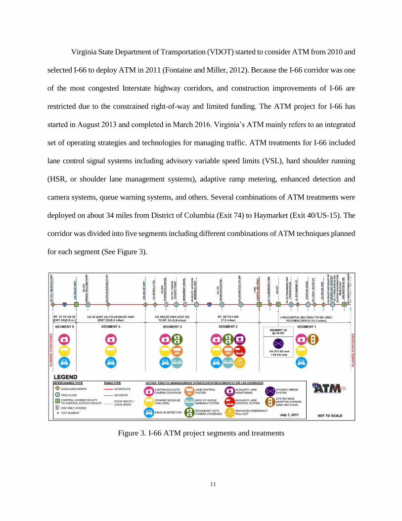
Virginia State Department of Transportation (VDOT) started to consider ATM from 2010 and
selected I-66 to deploy ATM in 2011 (Fontaine and Miller, 2012). Because the I-66 corridor was one
of the most congested Interstate highway corridors, and construction improvements of I-66 are
restricted due to the constrained right-of-way and limited funding. The ATM project for I-66 has
started in August 2013 and completed in March 2016. Virginia’s ATM mainly refers to an integrated
set of operating strategies and technologies for managing traffic. ATM treatments for I-66 included
lane control signal systems including advisory variable speed limits (VSL), hard shoulder running
(HSR, or shoulder lane management systems), adaptive ramp metering, enhanced detection and
camera systems, queue warning systems, and others. Several combinations of ATM treatments were
deployed on about 34 miles from District of Columbia (Exit 74) to Haymarket (Exit 40/US-15). The
corridor was divided into five segments including different combinations of ATM techniques planned
for each segment (See Figure 3).
Figure 3. I-66 ATM project segments and treatments
Page 35
12
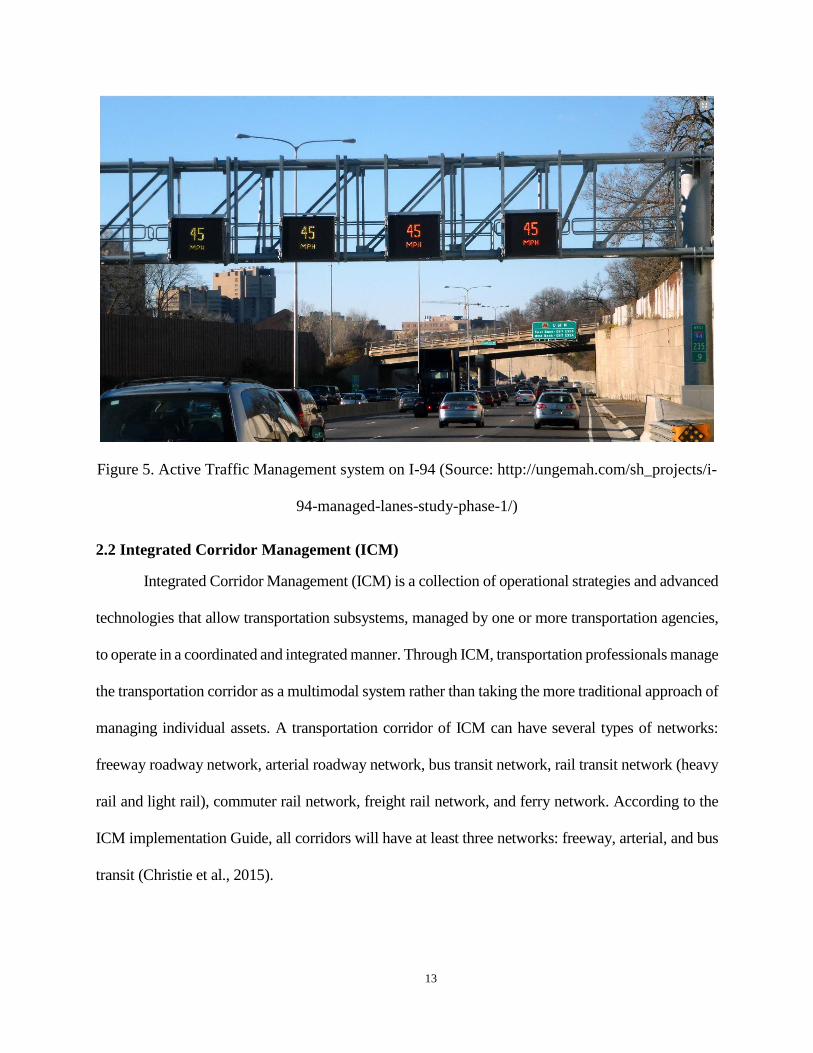
The ATM of Minnesota Department of Transportation (MnDOT) was introduced as part
of their priced dynamic shoulder lane project called Minnesota’s Smart Lanes (MnDOT, Fuhs,
2010). MnDOT is operating the ATM system within eighteen-mile section on Interstate 35 West
(I-35W) in the Twin Cities Metro Area and within eight-mile section on Interstate 94 (I-94)
between downtown Minneapolis and downtown St. Paul (FHWA, 2017b). The ATM on I-35W
was deployed to provide dynamic speed limit, dynamic shoulder lane, and dynamic lane assignment
for HOT through a series of overhead signs known as Intelligent Lane Control Signals (ILCS) (See
Figure 4). The ILCS is controlled through a freeway traffic management system software known
as Intelligent Roadway Information System (IRIS), which also controls loop detectors, DMS, and
ramp meters. ATM on I-94 is located between I-35W and I-35E and is providing advisory variable
speed limits, traffic control messages using lane control systems, and queue warnings (See Figure 5).
Figure 4. Intelligent lane control signals on I-35W
Page 36
13
Figure 5. Active Traffic Management system on I-94 (Source: http://ungemah.com/sh_projects/i-
94-managed-lanes-study-phase-1/)
2.2 Integrated Corridor Management (ICM)
Integrated Corridor Management (ICM) is a collection of operational strategies and advanced
technologies that allow transportation subsystems, managed by one or more transportation agencies,
to operate in a coordinated and integrated manner. Through ICM, transportation professionals manage
the transportation corridor as a multimodal system rather than taking the more traditional approach of
managing individual assets. A transportation corridor of ICM can have several types of networks:
freeway roadway network, arterial roadway network, bus transit network, rail transit network (heavy
rail and light rail), commuter rail network, freight rail network, and ferry network. According to the
ICM implementation Guide, all corridors will have at least three networks: freeway, arterial, and bus
transit (Christie et al., 2015).
Page 37
14
The ICM has four primary goals to increase corridor throughput, improve travel time
reliability, improve incident management, and enable intermodal travel decisions. The ICM provides
the following capabilities:
To deal with congestion and travel time reliability within specific travel corridor.
To optimize the use of existing infrastructure assets and leverage unused capacity along
our nation’s urban corridors.
To support transportation network managers and operators
In particular, the ICM concentrate on the following behaviors:
Daily operations (no incident)
Major freeway incident
Major arterial incident
Transit incident
Special event
Disaster response scenario
The ICM has four strategic areas: demand management, load balancing, event response, and
capital improvement. Demand management deals with patterns of usage of transportation networks.
Load balancing handles how travelers use the transportation networks in a corridor. Events can be
classified either by their duration or by their effects: reduction of capacity, increase in demand, or
change in demand pattern. Major improvement may be required to solve corridor-related traffic
problems in the long-term perspective (Christie et al., 2015). Major stakeholders interacting with the
ICM correspond on five areas: travelers and other transportation network users, commercial and
government entities, transportation network operators and their staff, public safety personnel, and
Page 38
15
other service providers. Several interfaces with the ICM are media feeds, Dynamic Message Signs
(DMS), Highway Advisory Radio (HAR), 511 systems, and traffic and transit web sites (Christie et
al., 2015).
Several key aspects for the successful ICM program were identified as institutional integration
including inter-agency cooperation and funding, technical integration including traveler information
and data fusion, and operational integration having performance measures and decision support
system. Thus, an institutional partnership is needed among the operating agencies, basic ITS
infrastructure and technology should be coordinated, and the agencies within the corridor need a
cooperative operational mindset (Spiller et al., 2014). Multiagency information sharing can be
accomplished through manual methods or through systems that are automated. ITS standards-based
C2C (Center to Center) systems were used to share data automatically (Spiller et al., 2014). Traveler
information is provided to the public through 511 services, web sites, media feeds, mobile
applications, and personalized information (Spiller et al., 2014).
Decision Support System (DSS) for ICM identifies sudden or pending nonrecurring events or
atypical recurring congestion beyond the norm via predictive modeling, and finds a best alternative
among various ICM strategies. The Dallas ICM system uses expert rules system to select a pre-agreed
response plan based on numerous variables and then uses a real-time model to validate that the
selected plan will provide a benefit. The San Diego system relies on its real-time model much more
and allows the model to use engineering principles and algorithms to generate a response plan for an
event within the corridor. The system has the capability to be fully automated or fully manual in
responding to the event (Spiller et al., 2014).
Page 39
16
In the first stage, the eight Pioneer Sites developed their Concept of Operations and System
Requirements Specification. In the second stage, three sites – Dallas, Minneapolis, and San Diego –
were selected to model the potential impact of ICM on their corridors. In the third stage, two sites –
Dallas and San Diego – were selected as ICM Pioneer Demonstration Sites to design, build, operate,
and maintain their respective ICMSs (Integrated Corridor Management Systems) and evaluate the
impact on the corridors. Currently, several states are trying to implement ICM systems. In case of
Florida, two projects are on-going: I-95 ICM in Broward County and I-4 ICM in Orlando.
2.3 Decision Support Systems (DSS)
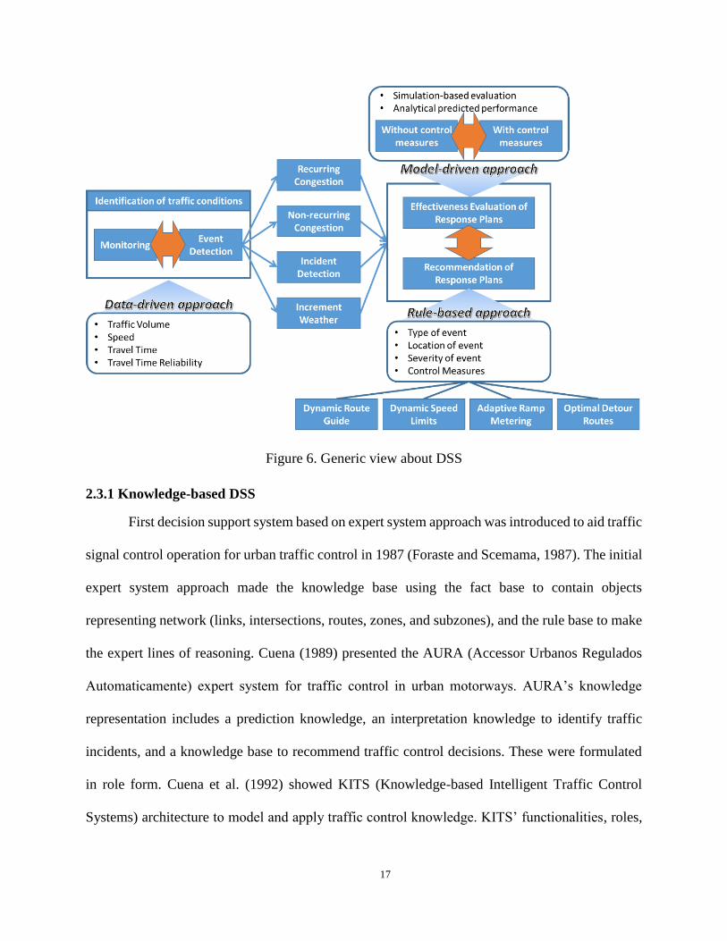
Decision Support Systems have been developed and used to assist operators’ decision-
making in various traffic circumstances. Casas et al. (2014) presented today’s generic architecture
of decision support systems for traffic management systems, which consists of several components:
real-time data, historical data, monitoring, predictive system, and strategy analysis (see Figure 6).
The real-time data include all kinds of data such as traffic data, weather data, incidents, special
events and so on. The historical data is to be accumulated from the real-time data. The monitoring
identifies and classifies the state of traffic network in real time. The predictive system is to predict
the state of traffic networks through analytical models and simulation-based models using real
time data and historical data. Finally, strategy analysis is to determine a set of strategies and
recommend a best strategy through a set of performance measures for the strategy evaluation.
Selecting a set of strategies depends on the operators’ knowledge and indicators evaluating
strategies can be determined in various.
Page 40
17
Figure 6. Generic view about DSS
2.3.1 Knowledge-based DSS
First decision support system based on expert system approach was introduced to aid traffic
signal control operation for urban traffic control in 1987 (Foraste and Scemama, 1987). The initial
expert system approach made the knowledge base using the fact base to contain objects
representing network (links, intersections, routes, zones, and subzones), and the rule base to make
the expert lines of reasoning. Cuena (1989) presented the AURA (Accessor Urbanos Regulados
Automaticamente) expert system for traffic control in urban motorways. AURA’s knowledge
representation includes a prediction knowledge, an interpretation knowledge to identify traffic
incidents, and a knowledge base to recommend traffic control decisions. These were formulated
in role form. Cuena et al. (1992) showed KITS (Knowledge-based Intelligent Traffic Control
Systems) architecture to model and apply traffic control knowledge. KITS’ functionalities, roles,
Page 41
18
and modeling approach were presented (Boero et al., 1994, Cuena et al., 1994, Boero, 1993, Cuena
et al., 1992). For adaptive traffic management systems, Cuena et al. (1995) proposed a general
structure for real-time traffic management support using knowledge-based models. The decision
support model for real-time traffic management is based on agent models and used traffic signal
operations and VMS (Variable Message Signboard) as treatments of traffic management.
Especially, a traffic simulator was used to build traffic models in the offline mode. To enhance
agent-based models, Hernandez et al. (2002) proposed multi-agent architectures for intelligent
traffic management systems including congestion warning, weather information, incident
notification with diversion of traffic, speed control and so on. Ossowski et al. (2005) presented an
abstract architecture for multi-agent DSS and showed examples to deal with real-world problems.
Considering a new conceptual architecture, Dunkel et al. (2011) proposed a reference architecture
for event-driven traffic management systems.
To provide decision support for traffic management center operators in integrated freeway
and arterial traffic management systems, Ritchie suggested a knowledge-based decision support
architecture, using a new artificial intelligence-based solution approach, for advanced traffic
management (Ritchie, 1990). Considered main functions are incident detection by algorithmic
methods, incident verification by CCTV, identification and evaluation of predefined alternative
responses and actions, implementation of selected response(s), and monitoring recovery through
the selected measures of effectiveness (MOE’s). Representative possible responses are as follows:
Modifying surface street signal timing plans
Initiating ramp metering changes
Coordination of ramp meters and surface street traffic signal timing
Activating freeway major incident traffic management teams
Page 42
19
Locating and activating freeway mobile and ground-mounted changeable message
signs (including composition of messages)
Activating changeable message signs on surface streets and approaches to freeways
access ramps (including composition of messages)
Selecting and implementing signed traffic detours
and so on
2.3.2 DSS using real-time traffic simulation
Some experts concentrated on research of decision support systems for effective traffic
incident management. Hu et al. (2003) proposed a real-time evaluation and decision support
system for incident management, which is composed of preprocess module, decision support
module and monitoring module (see Figure 7). The preprocess module has three functions: data
screening, data fusion, and incident detection. The decision support module includes neural-
network-based expert system, which can overcome the fuzziness of decision-making in rule-based
expert systems, data mining, real-time microscopic traffic simulation (PARAMICS; PARAllel
MICroscopic Simulator) to estimate the impacts of the incident (e.g. delay and queue length), and
comprehensive evaluation. The monitoring module has functions of traffic monitoring and
before/after evaluation. The neural networks have self-study abilities in adjusting their own
parameters to changing situations.
Page 43
20
Figure 7. Working process of the real-time evaluation and decision support system (Hu et al.,
2003)
Similarly, Chen et al. (2005) suggested a self-learning-process based decision support
system, which contains expert knowledge-based choice, case-based reasoning, and real-time
simulation, for Beijing traffic management. A mesoscopic large-scale network dynamic simulation
was used to identify problems and evaluation was performed by indicators. The simulation is based
on Dynamic Traffic Assignment (DTA) technology.
Shah et al. (2008) proposed a system architecture of a decision support system for freeway
incident management in Republic of Korea, which is based on traffic simulation. The main
function of the decision support system is to predict impacts of traffic incidents by using traffic
volume and speed. There was no explanation of decision support algorithms or techniques.
Page 44
21
For weather responsive traffic signal operations, Kim et al. (2014) developed real-time
simulation-based decision support system to reduce the impact of weather and keep the target
network service level (see Figure 8). The decision support system consists of real-time traffic
estimation and prediction system (TrEPS), scenario manager, and scenario library. The TrEPS,
which prototype is DYNASMART-X (Mahmassani, 1998) and DynaMIT-R (Ben-Akiva et al.,
1998), estimates current traffic conditions and predicts the future traffic conditions with or without
an alternative control strategy. The scenario manager provides functions to identify and assess
alternative signal control strategies based on TrEPS-predicted network states. The scenario library
stores predetermined weather-responsive signal timing plans, which the scenario manager uses in
real-time. As performance measures to decide an alternative traffic signal control, mean travel
time, total travel time, mean stopped time, and standard deviation of travel time were used.
Figure 8. Framework of TrEPS-based decision support system for weather-responsive traffic
signal operations (Kim et al., 2014)
Page 45
22
Still, real-time traffic simulation has a limitation which is to analyze many strategies in real
time within allowable computational budgets. Osorio and Bidkhori (2012) proposed a simulation-
based optimization (SO) algorithm to execute on-line traffic simulation under few runs. The
simulation-based optimization algorithm uses a Metamodel approach combining information from
the simulation model with information from an analytical probabilistic traffic model, which is a
network model based on finite capacity queueing theory.
Page 46
23
2.3.3 Case-based DSS without real-time traffic simulation
Although many decision support systems have used real-time traffic simulation, simulating
various traffic scenarios for many control measures in complicated traffic situations is difficult to
provide operators with the best control strategy on time. So, case-based decision support systems
were proposed (Hoogendoorn et al., 2003, Hegyi et al., 2001). The case-based approach has an a-
priori database including most of cases with traffic conditions and control scenarios. When a traffic
incident occurs, the real traffic condition is used to find the several cases in the database. Scenarios
in the cases are generated by traffic simulation. The alternative control measures with the best
performance in terms of a selected objective function can be recommended. Hegyi et al. (2001)
proposed a fuzzy decision support system for traffic control centers in order to optimize the number
of combinations of traffic control measures. The fuzzy case-based system can provide ranking of
control scenarios based on traffic conditions and control objectives. METANET macroscopic
traffic simulation was used to generate control scenarios (cases) with performance measures.
Furthermore, Hoogendoorn et al. (Hoogendoorn et al., 2003) developed a prediction system, which
is referred to as Fuzzy Multi-Agent Case-Base Reasoning, to forecast the effects of many candidate
control scenarios under the recurrent and non-recurrent traffic conditions in the network. So, the
prediction system uses case-based approach, fuzzy logic, and agent-based approach. METANET
simulation was used to create cases with performance measures and evaluate the decision support
system. Almejalli et al. (Almejalli et al., 2007) extended the idea of the fuzzy decision support
system into the fuzzy neural network in order to organize and initialize the fuzzy sets and
membership functions. Figure 9 shows the overall structure of the proposed system. METANET
was also used to train the developed model.
Page 47
24
Figure 9. Overall structure of the intelligent traffic control decision support system
(Almejalli et al., 2007)
2.3.4 Other DSS
As a part of DSS, Klein et al. (2002) developed a decision support system through more
advanced data fusion algorithm using the Dempster-Shfer theory to detect traffic events that occur
normal traffic operations. Related to generating traffic incident response plan automatically, Ma
et al. (2014) developed a method to build traffic incident response plan by using case-based
reasoning and Bayesian theory. Kim et al. (2017) developed an integrated multi-criteria support
system for assessing detour decisions during non-recurrent freeways congestion. The integrated
multi-criteria support system is based on the prediction algorithm of incident clearance times and
analytical hierarchy process (AHP).
In addition, decision support systems for effective and safe work zone management were
developed. Adeli (2004) conducted to develop an intelligent decision support system for work
Page 48
25
zone traffic management and planning, which focused on developing models: Case-based
reasoning model for freeway work zone traffic management, freeway work zone traffic delay and
cost optimization model, radial basis function neural network for work zone capacity and queue
estimation, neuro-fuzzy logic model for freeway work zone capacity estimation; object-oriented
model for freeway work zone capacity and queue delay estimation; and clustering-neural network
models and parametric study of work zone capacity. Paisalwattana and Tanaboriboon (2005)
presented a decision support system for work zone safety management in Thailand, which is to
help design and select safe and proper traffic control for work zone. The DSS used the fact-rule-
solution relationships of work zone management system and developed according to the following
steps: problem identification; database conceptualization, and model formalization.
Page 49
26
2.4 Travel Time Reliability
2.4.1 Measures of travel time reliability
Based on the previous research (Taylor, 2013, Chase Jr et al., 2013, Haghani et al., 2014,
Van Lint et al., 2008, Lomax and Margiotta, 2003), travel time reliability metrics were selected
within four classifications, which are statistical range measures, buffer time measures, tardy-trip
measures, and probabilistic measures. Currently, several agencies are using different travel time
reliability measures considering their own mobility policies. These measures can also be
distinguished by robust statistics, which are insensitive to the effects of outliers or events, and non-
robust statistics. The robust statistics are based on medians instead of means and use more
information from the center than from the outlying data (2017). A skew statistic, width statistic,
buffer index based on median and probabilistic measures use robust statistics.
2.4.1.1 Statistical Range Measures
Statistical range measures include standard deviation (SD), coefficient of variation (CV),
skew statistic (𝜆𝑠𝑘𝑒𝑤) and width statistic (𝜆𝑣𝑎𝑟), which are an attempt to quantify travel time
reliability in a statistical perspective. The CV is one metric to measure data variability, which can
be used to identify links or corridors to experience the higher travel time variation over long
periods of time than other links (Turner et al., 2011a). According to analytic relationships between
travel time measures, the CV is a good proxy for planning time index, median-based buffer index,
and skew statistic (Pu, 2011). The skew statistic and the width statistic follow the concept that
asymmetric, wider, and larger distribution relative to median will be able to be unreliable (Van
Lint and Van Zuylen, 2005). Thus, the two statistics should be considered together for travel time
reliability.
𝐶𝑉 = 𝑆𝐷/𝑚𝑒𝑎𝑛(𝜇) × 100
Page 50
27
𝜆𝑠𝑘𝑒𝑤 =𝑇𝑇90𝑡ℎ−𝑇𝑇50𝑡ℎ
𝑇𝑇50𝑡ℎ−𝑇𝑇10𝑡ℎ ; 𝜆𝑣𝑎𝑟 =
𝑇𝑇90𝑡ℎ−𝑇𝑇10𝑡ℎ
𝑇𝑇50𝑡ℎ
where 𝑇𝑇90𝑡ℎ, 𝑇𝑇50𝑡ℎ, and 𝑇𝑇10𝑡ℎ stand for the 90th, 50th, and 10th percentile travel time,
respectively. Although FHWA does not recommend to use statistical range measures since it is not
easy for the public to understand, Van Lint and Van Zuylen (2005) used the skew statistic and
width statistic of the day-to-day travel time distribution in order to monitor and predict freeway
travel time reliability.
2.4.1.2 Buffer Time Measures
As buffer time measures, buffer index (BI) based on average, BI based on median, and
planning time index (PTI) were selected. The BI implies that as a traveler should allow an extra
percentage of travel time to arrive at a destination on time, and the PTI provides an expected travel
time budget, which could be used as a trip planning measure for journeys that require punctuality
(Lomax and Margiotta, 2003). FHWA, Georgia Regional Transportation Authority, Georgia
Department of Transportation (DOT), and Maryland State Highway Administration (MSHA)
introduced BI and PTI to represent travel time reliability (FHWA, 2006). Florida DOT and the
National Transportation Operations Coalition (NTOC) are using BI (Turner et al., 2011b).
Washington State DOT chose PTI to provide the best time for travelers to leave (WSDOT, 2017).
𝐵𝐼𝑚𝑒𝑎𝑛 =𝑇𝑇95𝑡ℎ−𝐴𝑣𝑒𝑟𝑎𝑔𝑒 𝑇𝑟𝑎𝑣𝑒𝑙 𝑇𝑖𝑚𝑒
𝐴𝑣𝑒𝑟𝑎𝑔𝑒 𝑇𝑟𝑎𝑣𝑒𝑙 𝑇𝑖𝑚𝑒× 100(%)
𝐵𝐼𝑚𝑒𝑑𝑖𝑎𝑛 =𝑇𝑇95𝑡ℎ−𝑀𝑒𝑑𝑖𝑎𝑛 𝑇𝑟𝑎𝑣𝑒𝑙 𝑇𝑖𝑚𝑒
𝑀𝑒𝑑𝑖𝑎𝑛 𝑇𝑟𝑎𝑣𝑒𝑙 𝑇𝑖𝑚𝑒× 100(%)
𝑃𝑇𝐼 =𝑇𝑇95𝑡ℎ
𝑇𝑇𝑓𝑟𝑒𝑒 𝑓𝑙𝑜𝑤 𝑜𝑟 𝑝𝑜𝑠𝑡𝑒𝑑 𝑠𝑝𝑒𝑒𝑑 𝑙𝑖𝑚𝑖𝑡
Page 51
28
2.4.1.3 Tardy Trip Measures
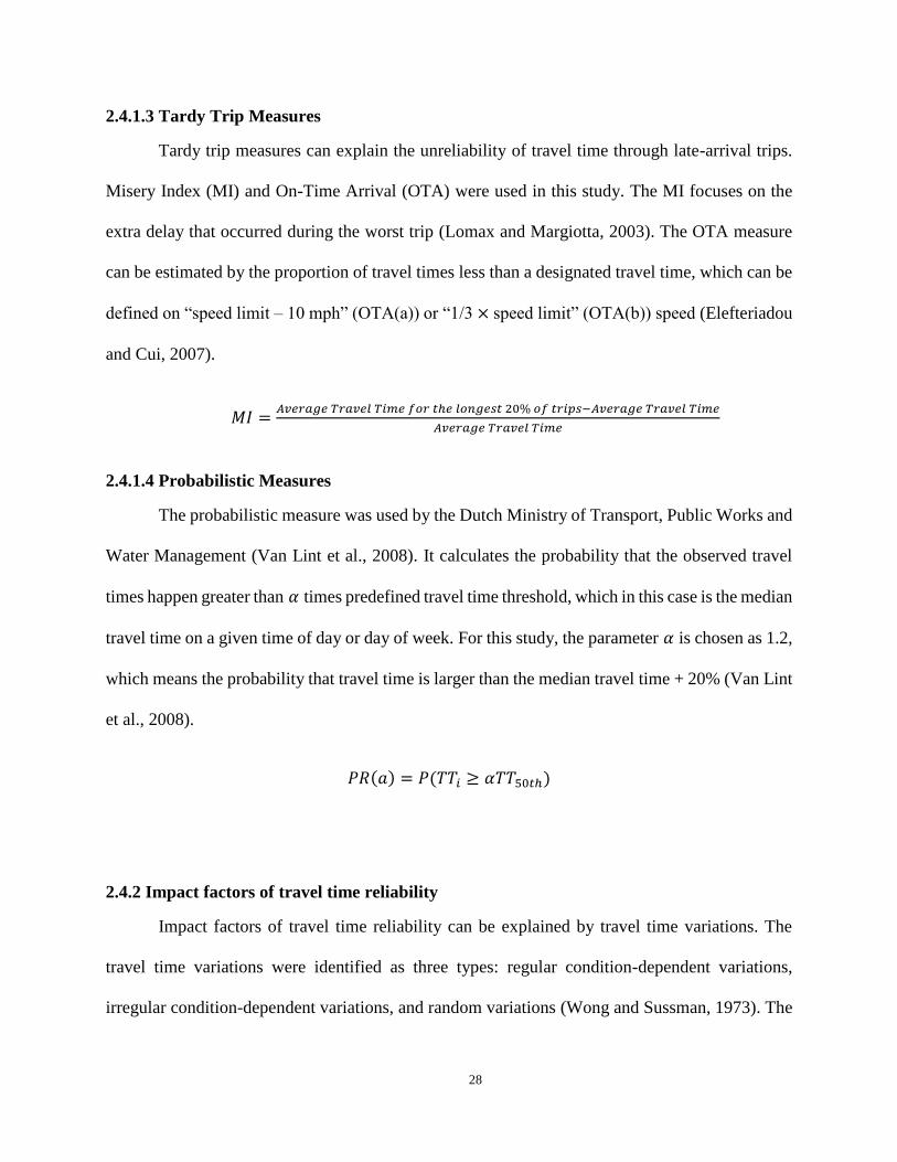
Tardy trip measures can explain the unreliability of travel time through late-arrival trips.
Misery Index (MI) and On-Time Arrival (OTA) were used in this study. The MI focuses on the
extra delay that occurred during the worst trip (Lomax and Margiotta, 2003). The OTA measure
can be estimated by the proportion of travel times less than a designated travel time, which can be
defined on “speed limit – 10 mph” (OTA(a)) or “1/3 × speed limit” (OTA(b)) speed (Elefteriadou
and Cui, 2007).
𝑀𝐼 =𝐴𝑣𝑒𝑟𝑎𝑔𝑒 𝑇𝑟𝑎𝑣𝑒𝑙 𝑇𝑖𝑚𝑒 𝑓𝑜𝑟 𝑡ℎ𝑒 𝑙𝑜𝑛𝑔𝑒𝑠𝑡 20% 𝑜𝑓 𝑡𝑟𝑖𝑝𝑠−𝐴𝑣𝑒𝑟𝑎𝑔𝑒 𝑇𝑟𝑎𝑣𝑒𝑙 𝑇𝑖𝑚𝑒
𝐴𝑣𝑒𝑟𝑎𝑔𝑒 𝑇𝑟𝑎𝑣𝑒𝑙 𝑇𝑖𝑚𝑒
2.4.1.4 Probabilistic Measures
The probabilistic measure was used by the Dutch Ministry of Transport, Public Works and
Water Management (Van Lint et al., 2008). It calculates the probability that the observed travel
times happen greater than 𝛼 times predefined travel time threshold, which in this case is the median
travel time on a given time of day or day of week. For this study, the parameter 𝛼 is chosen as 1.2,
which means the probability that travel time is larger than the median travel time + 20% (Van Lint
et al., 2008).
𝑃𝑅(𝑎) = 𝑃(𝑇𝑇𝑖 ≥ 𝛼𝑇𝑇50𝑡ℎ)
2.4.2 Impact factors of travel time reliability
Impact factors of travel time reliability can be explained by travel time variations. The
travel time variations were identified as three types: regular condition-dependent variations,
irregular condition-dependent variations, and random variations (Wong and Sussman, 1973). The
Page 52
29
regular condition-dependent variations are predictable and repeatable changes by time-of-day,
day-of-week, and season of year. The irregular condition-dependent variations are unpredictable
cases in traffic incident conditions such as adverse weather, traffic crashes, road work and so on.
The random variations represent the minor variations related to interactions between individual
drivers. To be specific, seven types of the impact factors were classified (Kwon et al., 2011):
Traffic incidents and crashes
Work zone activity
Weather and environmental conditions
Fluctuations in (day-to-day) demand
Special events
Traffic control devices, especially at-grade railway crossings and inappropriately
timed traffic signals and
Inadequate base capacity (i.e. traffic bottlenecks)
Most of the sources of traffic congestion are consistent with the above impact factors of
travel time reliability (Margiotta and Taylor, 2006). Thus, quantification of the impact of the above
types on travel time reliability is necessary to develop strategies to reduce traffic congestion.
Through empirical travel time reliability analyses, traffic incidents have a high impact on
travel time reliability through empirical analysis, and geometrical features and traffic controls have
the influence on travel time reliability (Tu et al., 2006, Wright et al., 2015, Tu et al., 2008). On the
contrary, Shi and Abdel-Aty (2016) investigated the impact of travel time reliability on crash
frequency using Bayesian hierarchical Poisson lognormal framework, and suggested that the
improvement of the travel time reliability might improve safety on expressways. Besides, it was
Page 53
30
confirmed that travel time reliability in work zones was degraded statistically significantly when
it was compared with the baseline group (Edwards and Fontaine, 2012). Especially, regarding the
impact on travel time reliability of weather, Tu et al. (2007) conducted empirical investigation
about weather impact on the travel time variability of freeway corridors, and showed that adverse
weather such as rain, snow, ice, fog and storm makes travel time unreliable although rain has little
or no effect on travel time below a certain critical inflow. Chien and Kolluri (2012) studied travel
time variability on New Jersey freeways by using TRANSMIT data, and found that the impact of
adverse weather on travel time reliability is more significant during peak periods than during off-
peak periods. Kwon et. al. (2011) found that weather has relatively little impact on travel time
unreliability, and weather is not significant for the “noon” period. Zhao and Chien (2012) analyzed
weather impact on travel time reliability, which is measured by BI, by using weather data of road
weather information system (RWIS) and speed data of INRIX. It was shown that adverse weather
make travel time reliability worse and the impact on the travel time reliability of precipitation
varies with the amount of precipitation (Zhao and Chien, 2012). Yazici et al. (2012, 2013)
investigated the impact of weather on travel time reliability in New York City and discovered that
travel time distribution patterns in New York City are different with freeways of the previous
research, and weather has a higher impact on travel time variability during less congested periods.
2.4.3 Estimation of travel time distribution or reliability
As travel time reliability has become an important part of traffic operation and management,
there have been many studies to estimate many kinds of travel time reliability through the modeling
of travel time distribution. Zheng et al. (2011, 2012, 2014) developed models to predict distribution
of link travel times for urban arterials by considering stochastic arrivals and departures at
signalized intersections, traffic signal timing, delay distribution, and queue distribution. Further,
Page 54
31
Chen et al. (2014) provided a finite mixture of regression model with varying mixing probabilities
to estimate urban arterial travel times through the travel time distribution considering traffic signal
timing at signalized intersections. Kim and Mahmassani (2015) proposed a method to model travel
time reliability through a compound representation of both vehicle-to-vehicle and day-to-day
variability, which is based on the product of two Gamma distributions. Kim et al. (2013) showed
an approach to build travel time distributions through scenario-based approach using traffic
simulation models, and performed scenario-based reliability analysis. The four scenarios were
considered: normal day, heavy rain only, accident only, and accident and heavy rain. Estimated
travel time reliability measures are standard deviation (min), coefficient of variation, 80th
percentile (min), 95 percentile (min), buffer index (%), buffer time (min), percentage on time (%),
and misery index. Park et al. (2011) made a three-state mixture travel time distribution model to
quantify the impact of traffic incidents on travel time reliability for freeways, using the
INTEGRATION microscopic traffic simulation software. Three states were defined as a non-
congestion, a medium-level congestion, and a medium level congestion, which were assumed to
follow normal distributions. The developed model was assessed by the 90th percentile travel times.
To identify network-level travel time reliability, Clark and Watling (2005) proposed an
analytic technique to estimate probability distribution of total network travel time based on a
standard traffic assignment model. The technique was proved through a conceptual example
network, and actual networks was not applied because of implementation issues such as
computational loads. Besides, Al-deek and Emam (2006) developed a methodology to estimate
link capacity reliability, link travel time reliability and network reliability, which are based on a
virtual small size network. The link travel time reliability is estimated through the Bureau of Public
Roads formula considering travel demand and capacity, and the network system reliability is the
Page 55
32
probability of the union of successful paths for a system. The developed link travel time and
network reliability models were tested on one corridor, Interstate 4, using dual-loop detector data
(Emam and Ai-Deek, 2006). As a similar concept, Tu et al. (2012) used risk assessment technique
to model travel time reliability and variability to identify the performance of transport systems. In
practical, Zheng et al. (2017) developed a network-level travel time distribution model through a
Johnson curve system and actual travel time data collected by Automated Number Plate
Recognition (ANPR) cameras. The network-level travel time distribution model showed the
possibility that the travel time reliability can be used as traffic management and control measures
through the relationship between network travel time reliability measures and network traffic
features such as network traffic density and flow.
Reliability and unreliability of travel time was applied to develop a new traffic equilibrium
model, which is called the alpha-reliable mean-excess traffic equilibrium (METE) model. The
METE model used travelers’ mean-excess travel times defined as the conditional expectation of
travel times beyond the travel time budget. The mean-excess travel times include the combination
of the buffer time measure and the tardy time measure to represent travelers’ behavior (Chen and
Zhou, 2010).
2.5 Summary
ATM strategies were introduced to automate and intensify advanced traffic management
related to traffic congestion and incident on freeways and expressways. Further, the concept of the
ATM strategies was extended to arterials using adaptive signal control systems. Even, ICM was
implemented in order to maximize the efficiency of the existing transportation systems by
integrating freeways, arterials, and transit networks. However, there are still research needs to
focus on.
Page 56
33
It is necessary to integrate freeways and arterials through the advanced new concept
as advanced traffic management systems have been more complicated.
Travel time reliability was not considered directly in strategies, algorithm, and DSS
of the ATM and ICM although previous ATM and ICM projects showed their
successful implementation and deployments in terms of travel time reliability’s
improvement.
Integrated Freeway/Arterial Active Traffic Management (IATM) should use a case-
based DSS without real-time traffic simulation because the real-time traffic
simulation cannot execute all kinds of combination of traffic control measures on
time in real time.
Page 57
34
CHAPTER 3. AVAILABILITY OF HERE DATA FOR TRAVEL TIME
RELIABILITY
Recently, private-sector data have been considered to estimate travel time reliability of
major road infrastructure. However, there is no study evaluating the difference of travel time
reliability between the private-sector data and Automated Vehicle Identification (AVI) based on
radio frequency identification. As ground truth data, the AVI data were collected from an AVI
system using toll tags and aggregated into 5-minutes intervals. As one of the representative traffic
information providers, the HERE data calculated in 5-minutes intervals were obtained through the
Regional Integrated Traffic Information System. For comparison, four kinds of measures were
selected and estimated on the basis of the day of the week, specific time periods, and time of day
in 5-minute, 15-minute, and one hour periods. The statistical difference in travel time reliability
was assessed through paired t-tests. According to the results, AVI and HERE data are comparable
based on day of the week, specific time periods, and time of day in one hour, whereas in the time
of day in 5-minute and 15-minute, HERE and AVI data are not generally comparable. Thus, when
estimating travel time reliability in real time, travel time reliability derived from HERE data may
be different from the true travel time reliability. Considering that private-sector traffic data can be
used to estimate travel time reliability measures, the measures should be harmonized on the basis
of robust statistics so that it can provide more consistent measures related to the true travel time
reliability.
3.1 Introduction
Many transportation researchers have been interested in travel time reliability to make
preparation for uncertainty due to unexpected traffic demand, crashes, and weather because travel
time reliability can provide buffers to sustain unfailing travel time for drivers, travelers, traffic
operators and even planners. For the past decades, they defined the concept of travel time reliability
Page 58
35
and developed several metrics and models with regard to it in various perspectives (Taylor, 2013).
Based on the metrics and models, diverse impact on factors of nonrecurring congestion has been
investigated. As a representative case, the Strategic Highway Research Program 2 (SHRP2) and
the Federal Highway Administration (FHWA) sponsored much research in travel time reliability
(TRB).
Basically, these research studies have used three types of traffic data sources:
infrastructure-based detectors such as loop and radar detectors, automated vehicle identification
(AVI) systems such as Bluetooth readers, license plate readers, and radio-frequency identification,
and automated vehicle location (AVL) systems tracking vehicle’s location (List et al., 2014).
Generally, the infrastructure-based detectors and the AVI systems have already been used in traffic
management systems of many regions, whereas the AVL systems have not been deployed fully to
provide sufficient data on a regional scale. As the data collection ability and coverage of the private
sector using AVL systems improve, some researchers started to use the private-sector traffic data
to study travel time reliability and to analyze its performance measures.
In 2011, the United States Department of Transportation (USDOT) started to consider
using the private sector data for national transportation performance management and several
public agencies jointly developed and published guidelines for evaluating the accuracy of travel
time and speed data of commercial traveler information services (Turner et al., 2011a, Turner et
al., 2011b). Among traffic information providers, HERE, INRIX, and TomTom were selected as
three highly qualified vendors in the I-95 Corridor Coalition’s Vehicle Probe Project (VPP) (VPP,
2017). The VPP has validated the three vendors’ data on freeways and arterials in four flow
regimes (0-30 mph, 30-45 mph, 45-60 mph, more than 60 mph) by using a Bluetooth technology.
The data quality measures were average absolute speed error (AASE) and Speed Error Bias (SEB)
Page 59
36
(2010). The qualified traffic data require that the AASE should be less than 10 mph and the SEB
should be within +/- 5 mph in each of the four-speed ranges. Nevertheless, there were not many
studies to use and validate the private-sector data for travel time reliability.
One study investigated travel time reliability in work zones by using 15-minute traffic data
of INRIX (Edwards and Fontaine, 2012). As travel time reliability measures, 95th percentile travel
time, a buffer index (BI) based on the average travel rate (minute/mile), and a planning time index
(PTI) were used. Through the travel time reliability measures, it was statistically quantified that
work zones have a negative impact on travel time reliability during non-peak periods as well as
peak periods. Furthermore, there was a detail analysis of thirteen travel time reliability measures
based on 15-minute space mean speed data of INRIX (Chase Jr et al., 2013). It was recommended
that ideal comparisons of reliability measures should use all 24 hours of the day and time of day
analysis should be conducted to find what time periods will be effective to improve travel time
reliability through traffic management strategies. Besides, it was shown that there is no single best
performance measure for travel time reliability and statistical range measures for travel time
reliability have the lowest correlation with the average travel rate than other measures.
At the same time, users including public agencies can still have a question whether the
travel time reliability performance measures can be trustfully estimated under the condition that
processing algorithms and quality assessment methods of private data sources are unknown (List
et al., 2014). Related to the question, one comparative study was conducted to analyze the effect
of data source selection on travel time reliability assessment by using 15-minute aggregation data
(Haghani et al., 2014). The research analyzed travel time reliability derived from Bluetooth and
INRIX data on interstate 95 (I-95) and interstate 207 (I-207) with HOV lanes. According to the
results, travel time reliability of I-95 is not statistically significantly different between the two data
Page 60
37
sources, but I-207 has significantly different travel time reliability because of HOV lanes. Thus, it
was found that some reliability metrics are more sensitive to the data source than others.
TomTom’s historical traffic data were evaluated in terms of travel time reliability through
a comparative study in Calgary, Canada (Tahmasseby, 2015). Travel time reliability was measured
by the 95th percentile travel time, the BI, the travel time index (TTI) and the PTI. Although this
study found that TomTom provides travel time reliability estimates with reasonable accuracy, the
validation was not proven statistically since the sample size was not adequate.
Apart from travel time reliability, there were several comparison or evaluation research
related to the travel time and speed of HERE. A comparison study of several data collection
methods to estimate travel time of freeways and arterials in Florida was conducted. According to
the research results, HERE provides more accurate travel times on freeways for oversaturated
conditions than INRIX and the Bluetooth system, but INRIX and Bluetooth are better than HERE
for uncongested periods (Elefteriadou et al., 2014). In the case of arterials, all methods were not
accurate. Furthermore, there were research comparing arterial speeds of Bluetooth, HERE and
INRIX in Southeast Florida to find alternatives for transportation planning measures (Rapolu and
Kumar, 2015). The study showed that Bluetooth and HERE data sets are similar, but INRIX speeds
are 5 to 10 mph lower than Bluetooth and HERE.
Recently, FDOT is trying to use multiple data sources for mobility performance measures,
such as travel time reliability, travel time variability, vehicle hours of delay and so on (FDOT,
2015b). In terms of data availability, cost-effectiveness, and usability of the multiple data sources,
the National Performance Measure Research Dataset (NPMRDS) and HERE, instead of TomTom
and INRIX, were chosen for the mobility performance measures of Florida. The research had a
Page 61
38
plan to evaluate and compare the estimated mobility performance measures, not with actual travel
time collected by other truthful systems, but the existing model based method. However, the
evaluation and comparison results have so far not been confirmed.
Whereas, this study aims to compare travel time reliability of HERE’s data with the actual
truthful system, the AVI system, which differs with the previous research using Bluetooth. The
AVI system uses toll tags, which provide much better, stable, and qualified data than Bluetooth.
For comparison, it explores travel time reliability performance measures based on several analysis
scenarios including each weekday of the year, time period of an average weekday, day of the week,
and time of day of an average weekday.
3.2 Study locations
Figure 10. AVI and HERE segments on Florida State Road 417
Six segments on Florida State Road 417 (SR 417) managed by Central Florida Expressway
(CFX) Authority operating with the speed limit of 70 mph were selected for the analysis because
it was found that locations of AVI readers are practically identical with the starting or ending points
Page 62
39
HERE segments (see Figure 10). Each AVI segment contains two to six segments of HERE and
has an average length of about 4 miles. The node information of HERE segments was collected
from the Regional Integrated Transportation Information System (RITIS) (CATT, 2008). The
road-widening construction has been underway within AVI S01 and N03 segments since
December 2015 (CFX, 2015).
3.3 Data Preparation
AVI data of 2016 were obtained from CFX’s AVI system archiving the encrypted tag IDs
and the passage timestamps of vehicles with toll tags since September 2012 (Abdel-Aty et al.,
2014). Uncapped raw AVI data, which is not adjusted by the speed limit, were archived for this
research and used because more tangible travel time can be estimated as ground-truth data. The
uncapped raw AVI data were aggregated in five-minute intervals and their outliers were eliminated
through the median absolute deviation (MAD) approach. The MAD approach provides a high
accuracy and low computational efforts (Leys et al., 2013). The removal criterion of outliers
becomes:
𝑀𝑒𝑑𝑖𝑎𝑛 − 𝑏 ∗ 𝑀𝐴𝐷 < 𝑡𝑟𝑎𝑣𝑒𝑙 𝑡𝑖𝑚𝑒(𝑖) < 𝑀𝑒𝑑𝑖𝑎𝑛 + 𝑏 ∗ 𝑀𝐴𝐷
where b is a threshold, in which 3 was applied very conservatively (Miller, 1991). In addition, it
was confirmed whether the count of the data used in each aggregation period satisfy the required
sample size, which is estimated by the following equation (May, 1990):
𝑛 = (𝑡𝑠
휀)
2
where n = required sample size
Page 63
40
s = standard deviation, which was estimated in each five-minute aggregation
휀 = user-specified allowable error, in which 5 mph was applied
t = 1.96 at 95 percent confidence was used
If the number of data in 5-minute increments is less than the required sample size, the
corresponding time periods were removed. Among one-year data, approximately 5-minute traffic
data of 7.2% were removed through the MAD approach.
The travel times of HERE, which were aggregated in five-minutes intervals, were
downloaded via the RITIS platform (Vandervalk, 2014). The raw travel times are generated
through data fusion processing of various data sources including state sensor data, probe vehicle
data, GPS data and historical data, but the traffic data processing algorithms are not published
(Elefteriadou et al., 2014). The data is estimated at Traffic Message Channel (TMC) segments,
which are divided at physical or logical geometric changes. Each AVI segment is composed of
several TMC segments (see Figure 10). On the basis of the AVI segments, each travel time of
TMC segments was added at five-minute intervals in order to be compared with AVI data. Finally,
all travel times of AVI and HERE were normalized by the distance of segments as follows (Jenks
et al., Lomax and Margiotta, 2003):
𝐴𝑐𝑡𝑢𝑎𝑙 𝑇𝑟𝑎𝑣𝑒𝑙 𝑅𝑎𝑡𝑒 (𝑚𝑖𝑛𝑢𝑡𝑒/𝑚𝑖𝑙𝑒) = 𝐴𝑐𝑡𝑢𝑎𝑙 𝑇𝑟𝑎𝑣𝑒𝑙 𝑇𝑖𝑚𝑒 (𝑚𝑖𝑛𝑢𝑡𝑒)
𝐷𝑖𝑠𝑡𝑎𝑛𝑐𝑒 𝑜𝑓 𝑠𝑒𝑔𝑚𝑒𝑛𝑡𝑠 (𝑚𝑖𝑙𝑒)
3.4 Analysis Scenarios
Travel time reliability measures can be calculated according to various viewpoints. For
example, the travel time reliability measures of each segment or corridor can be aggregated by day
of week (DOW), time period (TP) such as AM peak, PM peak, Mid-day, and late PM of an average
Page 64
41
weekday, and time of day (TOD) of an average weekday. They can also be separated and analyzed
depending on events including weather, incidents, and so on, but the events were not distinguished
in this study. With reference to previous research (Lomax and Margiotta, 2003), several analysis
scenarios were established as follow:
Average travel time reliability by DOW of the whole year: the travel time
reliability measures are aggregated for each DOW and analysis section.
Average travel time reliability by TP (AM Peak, Mid-day, PM Peak, and Late
PM) of an average weekday
Average travel time reliability by TOD in an hour intervals of an average
weekday
Average travel time reliability by TOD in 15-minute increments of an average
weekday
Average travel time reliability by TOD in 5-minute increments of an average
weekday
To analyze the difference of travel time reliability measures between the two data sources,
it is necessary to confirm whether travel time reliability measures derived from two data sources
are equal statistically. As a general statistical method, the paired t-test was applied.
3.5 Travel Time Data Distribution of AVI and HERE
This study concentrated on travel rates during weekdays of 2016, which can provide
obvious travel patterns with incidents such as crashes, road work, and adverse weather. After
abnormal data of AVI were removed through MAD approach and the statistical effective sample
size, scatter plots were used to confirm whether the overall tendency of travel times between AVI
Page 65
42
and HERE are similar. Figure 11 shows travel time patterns by the direction of SR 417. S01 and
N03 segments are the most congested in the southbound and northbound, respectively, due to the
road-widening construction since December 2015, and they have obvious AM and PM peak time
periods. Other segments also have a traffic pattern that travel rates increase during commuting
time periods, but the magnitude of the increment is much less than S01 and N03. Comparing scatter
plots of AVI with HERE, it seems that both AVI and HERE have similar traffic patterns although
some travel rates of HERE, which could have occurred under nonrecurring congestion during the
day, were estimated lower during the day and were spread more during the late night and early
morning than AVI data.
Page 66
43
Figure 11. Scatter plots of 5-minute travel rates for all segments
To observe additional features between AVI and HERE, cumulative distributions of travel
rates by direction were used. For the clear view, this study used average travel rates for 5-minute
time of day of an average weekday to make the cumulative distribution. According to the
cumulative distribution of all average travel rates for all times of day (see Figure 12-(a) and Figure
12-(c)), it is evident that the range of the average travel rate is different between the southbound
and northbound directions, so it is necessary to distinguish between both directions in the
comparative study.
Page 67
44
Figure 12. Empirical Cumulative Distributions (ECD) of average travel rate for time of day in 5-
minutes increment
More specifically, HERE data seem to fall behind AVI data until before a point of the first
tangency because HERE travel times were capped, but AVI travel times were not capped by the
speed limit of 70 mph, which is the travel rate of 0.867 minutes/mile. After the point of tangency,
in which the impact of the adjusted speed disappears, HERE and AVI data are moving in the same
trend although HERE underestimated some radically increased travel times due to events.
Additionally, the cumulative distributions of average travel rates during the AM and PM peaks
(see Figure 12-(b) and Figure 12-(d)) focus on the phenomenon after first intersecting points. It
shows again that HERE and AVI have similar travel rate distribution during peak hour periods,
Page 68
45
although HERE has a possibility to estimate lower travel times than the actual travel times.
Therefore, it is necessary that different traffic data sources be evaluated in terms of travel time
reliability as well as travel times because they can have different data distributions depending on
their own processing algorithms.
3.6 Analysis Results
By using travel times and rates of 2016 on SR 417 based on the analysis scenarios, four
types of travel time reliability measures between AVI and HERE were compared through the
paired t-test. As with the review of travel rate distributions, the paired t-test was conducted by
distinguishing southbound and northbound direction. The null hypothesis is that there is no
significant mean difference of travel time reliability performance measures between AVI and
HERE.
According to the results of the paired t-test of all data regardless of driving direction and
segments (see Table 2), SD, CV, MI, and OTA(a) represent that AVI and HERE are statistically
significantly different in all test scenarios. However, the skew statistics, the width statistics, BI
based on median, and PR (1.2) show that AVI and HERE are not different until TOD in an hour
increment. It seems that this kind of separation caused by characteristics of robust statistics.
Considering various travel time distribution under different traffic conditions (Guessous et al.,
2014), this result showed that travel time reliability measures with robust statistics can explain the
relationship better between different data sources having the same purpose.
Page 69
46
Table 2. All paired t-test results of travel time reliability measures between AVI and HERE
Test scenarios Statistical range measure Buffer time measure Tardy trip measure
PR(1.2) SD CV 𝜆𝑠𝑘𝑒𝑤 𝜆𝑣𝑎𝑟 𝐵𝐼𝑚𝑒𝑎𝑛 𝐵𝐼𝑚𝑒𝑑𝑖𝑎𝑛 PTI MI OTA(a) OTA(b)
DOW
p-value 0.000 0.000 0.292 * 0.060 * 0.313 * 0.502 * 0.478 * 0.002 0.623 * 0.000 0.456 *
t-value 7.230 6.690 1.070 1.950 -1.030 0.680 -0.720 3.470 0.500 -4.440 0.760
𝛥 0.812 0.224 0.171 0.038 -1.040 1.102 -0.015 0.041 0.003 -0.001 0.003
CI 0.582 0.155 -0.155 -0.002 -3.113 -2.216 -0.057 0.017 -0.009 -0.001 -0.006
1.042 0.292 0.497 0.078 1.033 4.420 0.027 0.065 0.014 0.000 0.012
DF 29 29 29 29 29 29 29 29 29 29 29
TP
p-value 0.000 0.000 0.718 * 0.699 * 0.110 * 0.586 * 0.041 0.040 0.181 * 0.021 0.442 *
t-value 6.120 5.880 -0.360 -0.390 -1.650 -0.550 -2.130 2.150 1.370 -2.440 -0.780
𝛥 0.754 0.211 -0.054 -0.004 -1.516 -0.710 -0.037 0.021 0.014 0.000 -0.004
CI 0.502 0.138 -0.354 -0.024 -3.395 -3.348 -0.072 0.001 -0.007 -0.001 -0.015
1.006 0.284 0.247 0.016 0.364 1.929 -0.002 0.041 0.035 0.000 0.007
DF 29 29 29 29 29 29 29 29 29 29 29
TOD
(Hour)
p-value 0.000 0.000 0.043 0.933 * 0.003 0.421 * 0.000 0.000 0.079 * 0.000 0.180 *
t-value 7.290 7.360 -2.040 -0.080 -3.020 -0.810 -4.330 4.450 1.770 -3.800 -1.350
𝛥 0.629 0.171 -0.178 0.000 -1.203 -0.444 -0.032 0.027 0.008 -0.001 -0.003
CI 0.458 0.125 -0.350 -0.009 -1.991 -1.533 -0.046 0.015 -0.001 -0.001 -0.006
0.799 0.217 -0.006 0.009 -0.416 0.644 -0.017 0.039 0.018 0.000 0.001
DF 143 143 143 143 143 143 143 143 143 143 143
TOD
(15-min)
p-value 0.000 0.000 0.000 0.565 * 0.000 0.060 * 0.000 0.000 0.001 0.000 0.017
t-value 8.860 9.230 -4.430 -0.580 -5.590 -1.880 -8.530 6.620 3.300 -5.350 -2.400
𝛥 0.454 0.120 -0.175 -0.001 -1.176 -0.474 -0.032 0.026 0.008 -0.001 -0.002
CI 0.353 0.095 -0.253 -0.005 -1.589 -0.969 -0.039 0.019 0.003 -0.001 -0.004
0.555 0.146 -0.097 0.003 -0.762 0.021 -0.024 0.034 0.013 0.000 0.000
DF 575 575 575 575 575 575 575 575 575 575 575
TOD
(5-min)
p-value 0.000 0.000 0.000 0.175 * 0.000 0.000 0.000 0.000 0.000 0.000 0.000
t-value 10.290 10.980 -7.390 -1.360 -9.450 -4.170 -15.440 8.070 5.580 -6.820 -3.690
𝛥 0.318 0.081 -0.181 -0.002 -1.225 -0.614 -0.033 0.023 0.008 -0.001 -0.002
CI 0.258 0.066 -0.229 -0.004 -1.479 -0.903 -0.037 0.017 0.005 -0.001 -0.003
0.379 0.095 -0.133 0.001 -0.970 -0.325 -0.029 0.029 0.011 0.000 -0.001
DF 1,727 1,727 1,727 1,727 1,727 1,727 1,727 1,727 1,727 1,727 1,727 * This indicates no rejection of the null hypothesis, there
is no mean difference between paired measures, at α =0.05.
𝛥: Mean difference
CI: Confidence Interval
DF: Degreed of Freedom
OTA(a): speed limit – 10 mph
OTA(b): 1/3 × speed limit
In the next analysis, the travel time reliability measures were compared by driving
directions. Table 3 shows the comparison results of the southbound direction and Table 4 is about
the northbound direction. Among statistical range measures of Tables 3 and 4, the standard
deviation and the coefficient of variance are statistically significantly different between AVI and
HERE in all test scenarios, whereas the width statistic (𝜆𝑣𝑎𝑟) are not statistically different in most
test scenarios except for TOD (5-minute). However, the skew statistic (𝜆𝑠𝑘𝑒𝑤) shows conflicting
Page 70
47
results in two different travel rate distributions. At least, the ratio of the range of travel times
between 90th percentile travel time and 10th percentile travel time and the median is statistically
consistent in AVI and HERE in all test scenarios except for TOD (5-minute).
Table 3. Paired t-test results of travel time reliability measures between AVI and HERE of the
southbound direction
Test scenarios Statistical range measure Buffer time measure Tardy trip measure
PR(1.2) SD CV 𝜆𝑠𝑘𝑒𝑤 𝜆𝑣𝑎𝑟 𝐵𝐼𝑚𝑒𝑎𝑛 𝐵𝐼𝑚𝑒𝑑𝑖𝑎𝑛 PTI MI OTA(a) OTA(b)
DOW
p-value 0.000 0.000 0.045 0.262 * 0.156 * 0.828 * 0.000 0.007 0.000 0.004 0.373 *
t-value 6.150 5.750 2.200 -1.170 -1.500 0.220 -6.000 3.160 7.870 -3.500 0.920
𝛥 0.829 0.233 0.191 -0.006 -0.847 0.138 -0.036 0.027 0.007 -0.001 0.001
CI 0.540 0.146 0.005 -0.017 -2.057 -1.200 -0.049 0.009 0.005 -0.001 -0.002
1.118 0.320 0.377 0.005 0.363 1.477 -0.023 0.045 0.009 0.000 0.005
DF 14 14 14 14 14 14 14 14 14 14 14
TP
p-value 0.002 0.002 0.115 * 0.737 * 0.658 0.589 * 0.009 0.022 0.001 0.005 0.451 *
t-value 3.800 3.690 1.680 -0.340 -0.450 0.550 -3.010 2.570 4.470 -3.360 0.780
𝛥 0.657 0.186 0.311 -0.003 -0.458 0.654 -0.033 0.024 0.008 -0.001 0.002
CI 0.286 0.078 -0.086 -0.021 -2.629 -1.880 -0.056 0.004 0.004 -0.001 -0.004
1.028 0.295 0.709 0.015 1.712 3.187 -0.009 0.043 0.012 0.000 0.009
DF 14 14 14 14 14 14 14 14 14 14 14
TOD
(Hour)
p-value 0.000 0.000 0.947 * 0.770 * 0.021 0.486 * 0.000 0.001 0.000 0.000 0.868 *
t-value 4.990 4.980 -0.070 -0.290 -2.360 -0.700 -6.430 3.530 3.900 -4.850 -0.170
𝛥 0.529 0.147 -0.005 -0.001 -1.112 -0.366 -0.038 0.022 0.007 -0.001 0.000
CI 0.317 0.088 -0.168 -0.011 -2.051 -1.408 -0.049 0.010 0.003 -0.001 -0.003
0.740 0.206 0.157 0.008 -0.173 0.676 -0.026 0.035 0.010 0.000 0.002
DF 71 71 71 71 71 71 71 71 71 71 71
TOD
(15-min)
p-value 0.000 0.000 0.485 * 0.399 * 0.000 0.403 * 0.000 0.000 0.000 0.000 0.828 *
t-value 6.570 6.670 -0.700 -0.840 -3.920 -0.840 -11.370 5.110 5.730 -6.740 0.220
𝛥 0.400 0.108 -0.030 -0.002 -1.024 -0.244 -0.037 0.021 0.007 -0.001 0.000
CI 0.280 0.076 -0.114 -0.007 -1.539 -0.818 -0.043 0.013 0.004 -0.001 -0.002
0.521 0.140 0.054 0.003 -0.509 0.330 -0.030 0.030 0.009 -0.001 0.002
DF 287 287 287 287 287 287 287 287 287 287 287
TOD
(5-min)
p-value 0.000 0.000 0.282 * 0.096 * 0.000 0.031 0.000 0.000 0.000 0.000 0.784 *
t-value 7.630 8.030 -1.080 -1.660 -6.750 -2.160 -20.060 5.910 8.900 -8.540 0.270
𝛥 0.285 0.074 -0.029 -0.003 -1.099 -0.368 -0.038 0.019 0.007 -0.001 0.000
CI 0.212 0.056 -0.082 -0.005 -1.419 -0.703 -0.042 0.013 0.005 -0.001 -0.001
0.358 0.092 0.024 0.000 -0.779 -0.034 -0.034 0.026 0.008 -0.001 0.001
DF 863 863 863 863 863 863 863 863 863 863 863 a This indicates no rejection of the null hypothesis, there
is no mean difference between paired measures, at α =0.05.
𝛥: Mean difference
CI: Confidence Interval
DF: Degreed of Freedom
OTA(a): speed limit – 10 mph
OTA(b): 1/3 × speed limit
In the buffer time measures, BI based on mean and BI based on median show a consistent
result in the two distributions. The BI based on mean has no difference between AVI and HERE
Page 71
48
in the only DOW and TP test scenarios, but the BI based on median has no difference in the DOW,
TP, TOD (Hour) and TOD (15-minute). On the other hand, PTI has no statistical difference
between AVI and HERE in only the North Direction's travel time distribution. The BI based on
median using one of the robust estimators shows that there is no difference between AVI and
HERE till the test scenarios from DOW to TOD (15-minute). This is the same result as the width
statistic. The only difference is that the width statistic uses 90th, 10th, and 50th percentile travel time,
and the buffer index is based on the median and uses the 95th and 50th percentile travel time.
Furthermore, it was found that all tardy travel measures are not different between AVI and
HERE in only the northbound travel time distribution with DOW, TP, and TOD (Hour) test
scenarios. Finally, the probabilistic measure, PR(1.2), had the same results in three test scenarios,
DOW, TP and TOD (Hour), on the distribution of both directions. PR(1.2) also uses the 50th
percentile travel time.
Page 72
49
Table 4. Paired t-test results of travel time reliability measures between AVI and HERE of the
northbound direction
Test scenarios Statistical range measure Buffer time measure Tardy trip measure
PR(1.2) SD CV 𝜆𝑠𝑘𝑒𝑤 𝜆𝑣𝑎𝑟 𝐵𝐼𝑚𝑒𝑎𝑛 𝐵𝐼𝑚𝑒𝑑𝑖𝑎𝑛 PTI MI OTA(a) OTA(b)
DOW
p-value 0.001 0.002 0.636 * 0.053 * 0.544 * 0.532 * 0.874 * 0.024 0.912 * 0.016 0.568 *
t-value 4.310 3.930 0.480 2.110 -0.620 0.640 0.160 2.530 -0.110 -2.730 0.580
𝛥 0.796 0.214 0.151 0.081 -1.233 2.065 0.007 0.055 -0.001 -0.001 0.005
CI 0.400 0.097 -0.519 0.163 -5.487 -4.845 -0.081 0.008 -0.025 -0.001 -0.013
1.192 0.331 0.821 -0.001 3.021 8.976 0.094 0.102 0.023 0.000 0.024
DF 14 14 14 14 14 14 14 14 14 14 14
TP
p-value 0.000 0.000 0.045 0.793 * 0.113 * 0.380 * 0.240 * 0.316 * 0.354 * 0.421 * 0.304 *
t-value 4.780 4.540 -2.200 -0.270 -1.690 -0.910 -1.230 1.040 0.960 -0.830 -1.070
𝛥 0.851 0.236 -0.419 -0.006 -2.573 -2.073 -0.041 0.018 0.020 0.000 -0.011
CI 0.469 0.124 -0.827 0.043 -5.836 -6.980 -0.113 -0.019 -0.024 -0.001 -0.032
1.232 0.347 -0.010 -0.055 0.690 2.834 0.031 0.056 0.064 0.000 0.011
DF 14 14 14 14 14 14 14 14 14 14 14
TOD
(Hour)
p-value 0.000 0.000 0.024 0.446 * 0.049 0.593 * 0.061 * 0.003 0.289 * 0.114 * 0.173 *
t-value 5.370 5.430 -2.310 0.770 -2.000 -0.540 -1.900 3.040 1.070 -1.600 -1.380
𝛥 0.729 0.195 -0.350 0.007 -1.295 -0.523 -0.026 0.031 0.010 0.000 -0.005
CI 0.458 0.123 -0.653 0.026 -2.583 -2.465 -0.052 0.011 -0.009 -0.001 -0.012
1.000 0.266 -0.047 -0.012 -0.007 1.419 0.001 0.052 0.029 0.000 0.002
DF 71 71 71 71 71 71 71 71 71 71 71
TOD
(15-min)
p-value 0.000 0.000 0.000 0.081 * 0.000 0.088 * 0.000 0.000 0.043 0.021 0.004
t-value 6.160 6.480 -4.890 1.750 -4.020 -1.710 -3.980 4.640 2.030 -2.330 -2.910
𝛥 0.507 0.132 -0.320 0.007 -1.328 -0.704 -0.026 0.032 0.010 0.000 -0.005
CI 0.345 0.092 -0.449 0.016 -1.978 -1.512 -0.040 0.018 0.000 -0.001 -0.008
0.669 0.172 -0.191 -0.001 -0.678 0.105 -0.013 0.045 0.020 0.000 -0.002
DF 287 287 287 287 287 287 287 287 287 287 287
TOD
(5-min)
p-value 0.000 0.000 0.000 0.011 0.000 0.000 0.000 0.000 0.001 0.004 0.000
t-value 7.130 7.640 -8.290 2.550 -6.690 -3.580 -7.310 5.710 3.460 -2.880 -4.360
𝛥 0.351 0.087 -0.332 0.006 -1.350 -0.859 -0.028 0.027 0.010 0.000 -0.005
CI 0.255 0.065 -0.411 0.011 -1.747 -1.330 -0.035 0.017 0.004 -0.001 -0.007
0.448 0.110 -0.253 0.001 -0.954 -0.388 -0.020 0.036 0.016 0.000 -0.002
DF 863 863 863 863 863 863 863 863 863 863 863 a This indicates no rejection of the null hypothesis, there
is no mean difference between paired measures, at α =0.05.
𝛥: Mean difference
CI: Confidence Interval
DF: Degreed of Freedom
OTA(a): speed limit – 10 mph
OTA(b): 1/3 × speed limit
Finally, the comparison of travel time reliability measures between AVI and HERE was
conducted for each segment (see Table 5). For this test, DOW and TP test scenarios were not
included because the sample size is too small. When the size of the interval of time of day is
decreased, the number of measures, representing two distributions are not different, is decreased.
Based on Table 5, travel time reliability measures of HERE are not different with AVI at most
Page 73
50
segments except for SB02 in TOD (Hour). The SB02 does not have any measure with p-value
more than 0.05 in all TOD, which means AVI and HERE data in the SB02 segment is definitely
different or there may be some error between AVI and HERE.
Table 5. Paired t-test results (p-value) of travel time reliability measures between AVI and
HERE of each segment
Test scenarios Statistical range measure Buffer time measure Tardy trip measure
PR(1.2) SD CV 𝜆𝑠𝑘𝑒𝑤 𝜆𝑣𝑎𝑟 𝐵𝐼𝑚𝑒𝑎𝑛 𝐵𝐼𝑚𝑒𝑑𝑖𝑎𝑛 PTI MI OTA(a) OTA(b)
TOD
(Hour)
NB01 0.002 0.002 0.051 * 0.664 * 0.012 0.380 * 0.600 * 0.009 0.381 * 0.002 0.406 *
NB02 0.060 * 0.043 0.091 * 0.323 * 0.042 0.093 * 0.000 0.808 * 0.050 * 0.838 * 0.053 *
NB03 0.001 0.001 0.309 * 0.079 * 0.763 * 0.462 * 0.251 * 0.031 0.086 * 0.855 * 0.972 *
SB01 0.010 0.010 0.332 * 0.061 * 0.468 * 0.185 * 0.333 * 0.005 0.112 * 0.003 0.412 *
SB02 0.000 0.000 0.001 0.003 0.000 0.000 0.000 0.028 0.000 0.004 0.000
SB03 0.136 * 0.131 * 0.452 * 0.617 * 0.145 * 0.220 * 0.000 0.730 * 0.006 0.047 0.349 *
TOD
(15-min)
NB01 0.000 0.000 0.000 0.360 * 0.000 0.116 * 0.328 * 0.000 0.111 * 0.000 0.159 *
NB02 0.034 0.020 0.015 0.064 * 0.000 0.003 0.000 0.495 * 0.000 0.988 * 0.000
NB03 0.001 0.001 0.009 0.000 0.846 * 0.403 * 0.043 0.003 0.003 0.795 * 0.425 *
SB01 0.000 0.000 0.164 * 0.002 0.102 * 0.005 0.144 * 0.000 0.019 0.000 0.096 *
SB02 0.000 0.000 0.000 0.000 0.000 0.000 0.000 0.001 0.000 0.000 0.000
SB03 0.038 0.035 0.163 * 0.247 * 0.009 0.030 0.000 0.605 * 0.000 0.006 0.154 *
TOD
(5-min)
NB01 0.000 0.000 0.000 0.128 * 0.000 0.003 0.053 * 0.000 0.019 0.000 0.080 *
NB02 0.009 0.003 0.000 0.001 0.000 0.000 0.000 0.533 * 0.000 0.913 * 0.000
NB03 0.001 0.001 0.000 0.000 0.827 * 0.371 * 0.002 0.001 0.000 0.891 * 0.292 *
SB01 0.000 0.000 0.045 0.000 0.047 0.000 0.002 0.000 0.000 0.000 0.008
SB02 0.000 0.000 0.000 0.000 0.000 0.000 0.000 0.000 0.000 0.000 0.000
SB03 0.043 0.037 0.244 * 0.050 * 0.000 0.000 0.000 0.710 * 0.000 0.004 0.093 * * This indicates no rejection of the null hypothesis, there is no mean difference between paired measures, at α =0.05.
OTA(a): speed limit – 10 mph
OTA(b): 1/3 × speed limit
Page 74
51
3.7 Conclusion
This study compared HERE data with AVI data using toll tags for electronic toll collection
and also providing sufficient sample size with high accuracy in terms of travel time reliability. So
far, traffic data of INRIX and TomTom as private sector data have been compared in terms of
travel time reliability, but HERE data has not been evaluated (Tahmasseby, 2015, Haghani et al.,
2014). In addition, these studies evaluated the private data using data at 15-minute intervals
because they use Bluetooth sensors that do not provide enough samples. On the other hand, this
study compared the reliability of travel time in more details using AVI's 5-minute interval data
with statistically sufficient samples.
In order to understand the characteristics of the travel-time data collected from AVI and
HERE, data of three sections by direction were combined. Scatter plots and cumulative empirical
distributions were used to visualize travel rates of AVI with HERE. Through the scatter plots, the
most congested sections and peak time periods were verified. The visualized cumulative
distributions showed the difference between capped speeds of HERE data and uncapped speeds of
AVI data. The difference disappeared at the first intersection points between the cumulative
distributions of AVI and HERE.
The selected travel time reliability measures for this study was divided into four groups,
statistical range measures, buffer time measures, tardy trip measures, and probabilistic measures.
According to the predefined test scenarios, all travel time reliability measures were estimated and
then tested through the paired t-test on whether the travel time reliability measures estimated from
the two data sources are statistically different or not. The test was conducted into two groups,
southbound travel times and northbound travel times.
Page 75
52
According to the statistical test results of the two groups, it was confirmed that the results
were different depending on elements of performance measures. It is shown that SD and CV, which
are representative of non-robust estimators using an average, have statistically significant
differences between AVI and HERE. In addition, most of the PTI, MI, and OTA using non-robust
estimators, average travel time, did not provide consistent evaluation results in AVI and HERE,
although BI based on mean travel times shows that the two data sources are not different in travel
time reliability of day of week and time periods of an average weekday. Conversely, it was found
that there is no statistical difference between AVI and HERE according to the test results of the
width statistic, buffer index based on median, and PR (1.2), which are using the robust estimator,
although the skew statistic did not yield a consistent conclusion in both distributions.
Considering the results of the previous research, robust statistics should be used for travel
time having compound distributions according to traffic conditions, there is no statistically
significant difference between HERE and AVI in terms of travel time reliability using day of the
week, time periods, and time of day in an hour unit. However, the travel time reliability measures
calculated from the two different data sources at 5 minute and 15 minute units can yield different
results. It is obvious that HERE data as a real-time feed will have differences with AVI data since
the HERE data can be estimated for all time periods through unopened modeling methods
including smoothing, filtering, and imputation using historical data when the collected data are
insufficient. The differences will be revealed more obviously when the aggregation time span
shortens. However, if raw traffic data without modeling will be used, the differences will be
reduced although there might be irreducible errors. On the other hand, on the basis of the average-
based BI, PTI, and OTA, which are currently used by public agencies in the USA, AVI and HERE
cannot estimate consistent travel time reliability measures.
Page 76
53
Based on the results of this study, travel time reliability measures should be changed to use
robust statistics such as median and percentiles. Thus, travel time reliability estimated through
different data sources can be consistent from a macroscopic perspective such as transportation
planning not real-time systems, such as Active Traffic Management strategies. This study
compared two different data sources in terms of travel time reliability using six short segments on
one corridor. This may not represent most of the freeways and expressways. For more general
conclusions, more types of road segments should be added and analyzed. Also changes in travel
reliability due to events should be studied in the future.
Page 77
54
CHAPTER 4. THE EFFECTIVE COVERAGE OF LAND-BASED
WEATHER STATIONS
This chapter investigates the effective spatial coverage of nationwide land-based weather
stations of the National Oceanic Atmospheric Administration (NOAA) for traffic crash analysis.
The weather data were collected from the Quality Controlled Local Climatological Data (QCLCD)
and the fatal crashes were obtained from the Fatality Analysis Reporting Systems (FARS) during
the year of 2007 to 2014. Both QCLCD and FARS contain geographic coordinates for locations
and weather condition information as a categorical variable. The spatial coverage of weather
stations for the analysis was made by geoprocessing, which uses multiple buffers (i.e. radii 5, 10,
15, and 20 miles), and then was evaluated via Cohen’s κ statistics, which is used to determine an
agreement of weather between QCLCD and FARS within the buffer. The applicability of the
weather station’s data by nine climate regions was assessed by developing a series of negative
binomial models. According to the estimated Cohen’s κ statistics, the rain and snow weather
conditions have a moderate agreement up to 20 miles. However, in the case of fog weather
condition, it has a slight agreement. The statistical modeling results showed that weather stations
data can be a good exposure measure for weather-related fatal crashes along with the vehicle-
miles-traveled. Considering one geographical feature that approximately more than 75% of all
fatal crashes are located within 20-miles radius of the weather stations in the USA, it is evident
that the data from the existing weather stations can be cost-effective to develop geospatial crash
risk analysis model.
4.1 Introduction
It is well known that weather has a significant impact on road transportation. For the
systematic weather-related research, the committee on weather research for the road transportation
Page 78
55
at the National Research Council of the National Academies (2004) had arranged a research agenda
for improving road weather services. The impact of weather on traffic operation has been
considered from the perspective of traffic flow (Maze et al., 2006) and traffic safety (Qiu and
Nixon, 2008, Andrey et al., 2001).
Regarding the impact of weather on traffic flow, there are many studies using weather data
which are collected from land-based weather stations near roadways (Ibrahim and Hall, 1994,
Cools et al., 2010, Smith et al., 2004, Agarwal et al., 2005, Hall and Barrow, 1988). These types
of studies verified that weather has an impact on highway capacity, speed, and density. As a result,
traffic engineers and operators have recognized quantified influences of weather on traffic flow
according to weather intensity from the land-based weather stations.
Furthermore, for the purpose of investigating the relationship between weather-related
crashes and weather, various studies have been conducted for several weather conditions. Some
studies conducted several comprehensive explorations using nationwide data in the United States
to understand the relationship between historical data of traffic crashes from the National Highway
Traffic Safety Administration (NHTSA) and archived weather data from the National Climatic
Data Center (NCDC) of the National Oceanic and Atmospheric Administration (NOAA)
(Eisenberg, 2004, Eisenberg and Warner, 2005, Pisano et al., 2008, Rossetti and Johnsen, 2011,
Ashley et al., 2015, Black and Mote, 2015a, Black et al., 2017). Other studies evaluated weather-
related crash risk based on hourly data provided by weather stations of NOAA, but the studies
were restricted to specific areas or roads (Abdel-Aty and Pemmanaboina, 2006, Black and Mote,
2015b, Black et al., 2017). Even, there was no study to confirm the quality of hourly weather data
collected by nationwide land-based weather stations in the USA.
Page 79
56
This study aims to assess the nationwide reliability of the hourly Quality Controlled Local
Climatological Data (QCLCD), which are the representative qualified weather data in the United
States. It uses contingency table analysis to match the NHTSA's FARS (Fatality Analysis
Reporting Systems) weather data (NHTSA, 2014) with the NOAA’s QCLCD data (NCEI, 2016)
to evaluate the usability of the QCLCD. This is achieved through the development of models to
estimate the number of annual fatal traffic crashes based on the duration of weather conditions,
and vehicle-miles-traveled (VMT)1 by weather conditions. Additionally, based on the developed
models and aggregated data, regional characteristics of weather-related fatal crashes are discussed.
4.2 Literature Review
With regards to nationwide rain-related and snow-related traffic crashes in the United
States, Eisenberg (2004) analyzed the mixed effects of precipitation, and Eisenberg and Warner
(2005) investigated the impact of snowfall. The study used fatal crashes for the 48 contiguous
states during 1975-2000, property-damage-only and injury crashes of 17 states during the 1990s
and daily state weather data from NCDC’s Cooperative Observer Network (COOP) (NCEI, 2016).
According to the results, snow days had fewer fatal crashes than dry days, but more injury crashes
and property-damage-only crashes. The first snow day of the year was substantially more
dangerous than other snow days regarding the number of fatalities, particularly for elderly drivers.
Also, the lagged effects of precipitation across days were found through nationwide weather-
related crash analysis.
Regarding the overall tendency analysis about US highway crashes in adverse weather
conditions, Pisano et al. (2008) handled weather exposure and severity and described statistics and
1 VMT = AADT (Annual Average Daily Traffic)× (segment length), vehicle-miles-traveled per day
Page 80
57
regional variance of weather-related crashes, injuries, and fatalities during 1995-2005. To confirm
regional variance of weather-related crashes, the authors used only mean total precipitation and
snowfall as weather information at the macroscopic level. Also, the authors confirmed that many
weather-related crashes occurred during rainfall or under wet pavement condition, and most
weather-related crashes take place in the South and the Midwest. To be specific, the South had
many rainfall- or wet-pavement-related crashes. On the other hand, the Midwest had relatively
more winter-weather-related crashes.
Further, related to the traffic safety policy of commercial vehicles, Federal Motor Carrier
Safety Administration (FMCSA) investigated weather-related fatal crash trends and climate-
change-related impacts through fatal crash data of FARS during 1975-2009 and climatic and
weather data from Storm Events Database (SED) of the National Climatic Data Center (NCDC)
(Rossetti and Johnsen, 2011). It is reported that all kinds of weather conditions can influence fatal
crashes of commercial vehicles, but when normalized by VMT, the fatal crash risk is less.
Moreover, the fatal crashes of commercial vehicles have a declining trend from 1975 to 2009, with
a leveling off since 1999. However, it was not possible to analyze a relation and a trend between
fatal crashes of commercial vehicles and weather events from SED because it includes only deaths
related to special weather phenomena.
Recently, Ashley et al. (2015) addressed a nationwide analysis of visibility-related fatal
crashes in the United States from 1994 to 2011. It showed that about 70% of visibility-related fatal
crashes occurred in the area without weather hazard advisories of the National Weather Service
(NWS). Additionally, Black and Mote (2015a) conducted another study about spatial and temporal
characteristics of winter-precipitation-related fatalities for the period 1975-2011. They reported
that the magnitude of fatalities caused by winter weather conditions is more than fatal counts
Page 81
58
reported from storm data of the NCDC for unusual weather phenomena. Both Ashley et al. (2015)
and Black and Mote (2015a) emphasized that measures for weather-related fatal crashes should be
established for different adverse weather conditions as well as special weather events.
In order to better figure out the impact of winter precipitation and rainfall on road traffic
crashes, Black and Mote (2015b) explored the impact of the winter precipitation on crashes in 13
cities in the United States. They used Automated Surface Observing System (ASOS) for weather
data and State Data System (SDS) for crash data during 1996-2010. It was confirmed that a higher
winter precipitation increases the numbers of traffic crashes and injuries, and the relative risks of
crash and injury rise when the intensity of the precipitation goes up. However, contrary to the result
of Eisenberg and Warner (2005), the relative risk of the first three precipitation events is not
different with subsequent precipitation events. In addition, Black and Villarini (2017) analyzed the
effects of rainfall on traffic crashes using gauge-based daily precipitation and NHTSA’s SDS of
six states in the USA during 1996-2010. It was proven that crash and injury rates increase during
rainfall between May and September, and the crash risk of crashes and injuries also rise. Both
studies showed that it is hard to explain all the relative risk of crashes due to the high precipitation
through only meteorological factors according to various spatial patterns or cities.
From a different angle, there have been efforts to assess or predict real-time crash risk using
archived weather data observed at airports’ weather stations. Abdel-Aty and Pemmanaboina (2006)
developed a real-time crash prediction model related to rainfall for the 36-mile freeway section on
I-4 in Central Florida through weather data from three airports. Moreover, Ahmed et al. (2014)
assessed the viability of airport weather data in real-time road crash risk assessment using eight
airports in the fog-prone area of Florida. Nevertheless, they did not investigate the feasibility of
weather stations’ data at the national level.
Page 82
59
4.3 Data Preparation
Three data sources were used for the nationwide weather data analysis: 1) weather data
from the hourly QCLCD (May 2007 to December 2014) (NCEI, 2017), 2) fatal crashes from
NHTSA’s FARS (2007 to 2014) (NHTSA, 2014), and 3) AADT from the Highway Performance
Monitoring System (HPMS) (2011 to 2012) (FHWA, 2014).
4.3.1 Nationwide QCLCD
Related to surface weather information, NOAA’s National Centers for Environmental
Information (NCEI) provides enormous weather observation data including Local Climatological
Data (LCD), Climatological Data (CD), Hourly Precipitation Data (HPD), Storm Data (SD),
COOP data and so on, which are observed from land-based stations. In the previous studies,
Eisenberg (2004), and Eisenberg and Warner (2005) utilized COOP data for monthly and daily
precipitation. Pisano et al. (2008) applied CD for mean total precipitation and snowfall. Rossetti
and Johnsen (2011), Ashley et al. (2015), and Black and Mote (2015a) used CD and SD for their
weather-related crash analysis. Abdel-Aty and Pemmanaboina (2006) used hourly rainfall data
from NOAA. Also, Ahmed et al. (2014) employed QCLCD (NCEI, 2016) to match weather
conditions observed at airports with the recorded weather-related crashes.
QCLCD is suitable for this study because it includes both categorical data and numerical
data related to all kinds of weather conditions every hour and whenever a weather-change event
occurs, whereas other weather data sources do not have direct categorical data for weather
conditions.
Page 83
60
Figure 13. Locations of weather stations in the USA
QCLCD on the NOAA’s official website were archived from 2,466 weather stations
operated between May 2007 and December 2014, and the number of observations is more than 3.3
billion counts (Figure 13). The weather stations include many types of land-based weather stations:
AWOS (Automated Weather Observing System), MAPSO (Microcomputer-Aided Paperless
Surface Observations), Navy METAR (METeorological Aerodrome Report), ASOS (Automated
Surface Observing System), CRN (Climate Reference Network) and so on. Data from 2,271
weather stations, which had fatal crashes within the radius of 20 miles from weather stations, were
extracted.
QCLCD’s hourly observations with variables include categorical variables such as weather
types as well as numerical variables such as precipitation, visibility, and wind speed. In this study,
only three variables, which are the date, time, and weather-type, were used to compare with the
weather-type variable of fatal crashes in the FARS database. All date and time were converted to
coordinated universal time (UTC) to identify the criteria of comparing time.
Page 84
61
4.3.2 Nationwide fatal crashes
This study amassed the nationwide fatal crashes of 2007-2014 from the FARS. Weather
types of FARS during 2010-2014 were also grouped according to the classification criteria of 2007-
2009 (NHTSA, 2015) (for consistency as criteria changed after 2009): Clear/Cloud,
Rain/Sleet/Hail, Snow or Blowing Snow, Fog/Smog/Smoke, Severe Crosswinds, and Blowing
Sand/Soil/Dirt. According to the frequency analysis of weather-related fatal crashes (see Table 6),
most weather-related fatal crashes, approximately 98%, took place in rain, snow, and fog weather
conditions and accounted for on average 11% of all fatal crashes. The proportions of fatal crashes
regarding severe crosswinds and blowing sand/soil/dirt are minuscule and even are smaller than
total cases of other, not reported, or unknown fatal crashes. Thus, we focused on rain-, snow-, and
fog-related fatal crashes.
Table 6. Weather-related fatal crashes by year (2007-2014)
Year
Weather Type 2007 2008 2009 2010 2011 2012 2013 2014 Mean
Clear/Cloud 32,281 29,519 26,759 26,576 26,098 27,366 26,256 26,356 27,651
Rain/Sleet/Hail 2,459 2,596 2,495 2,067 2,132 2,092 2,234 2,140 2,277
Snow or Blowing Snow 639 624 467 567 462 359 506 491 514
Fog/Smog/Smoke 408 408 303 293 325 364 372 318 349
Severe Crosswinds 74 55 46 41 49 55 51 47 52
Blowing Sand/Soil/Dirt 13 10 12 10 8 12 7 13 11
Other/Unknown 201 179 200 171 186 197 217 242 199
Total Fatal Crashes 36,075 33,391 30,282 29,725 29,260 30,445 29,643 29,607 31,054
Weather-related fatal
crashes ratio (%) 10.5 11.6 11.6 10.6 10.8 10.1 11.4 11.0 11.0
Ratio of rain, snow, and
fog among weather-
related fatal crashes (%)
97.6 98.2 98.3 98.3 98.1 97.7 98.2 98.0 98.0
Page 85
62
4.3.3 Nationwide AADT of the Highway Performance Monitoring System (HPMS)
National data sets of HPMS’s AADT data were collected from the Federal Highway
Administration. Although officially the national data sets are open from 2011 to 2014,
unfortunately, the national data sets in 2013 and 2014 had technical errors and could not be used
in this study. The national data set is based on national highway system (NHS) composed of
important roadways for the nation’s economy, defense, and mobility: interstate highways, other
principal arterials, strategic highway network, major strategic highway network connectors, and
intermodal connectors. Thus, the NHS does not include all kinds of roadways. For example, all
state highways or local roads are not allocated in the NHS.
Different from VMT for each state-year of the previous study (Eisenberg, 2004), this study
estimated more specific VMT by using AADT and segment length of highways within the specific
radius, e.g. 5 miles, from weather stations, that makes possible the weather-station-based analysis.
4.3.4 Grouping of weather types of QCLCD and FARS data
The weather classification of QCLCD and FARS is different since the QCLCD aims to
provide various stakeholders with more accurate and detail weather information and FARS
purpose to record the more simplified weather types for situation explanation of road traffic crashes.
Thus, this study reclassified weather types of the QCLCD and FARS to build contingency tables
according to several coverage radii. Through the FARS data preparation, it was confirmed that
average 98% of all weather-related fatal crashes occurred under the three major weather conditions:
rain, snow, and fog (see Table 6). Based on the majority of weather types related to fatal crashes,
all weather types of the QCLCD and FARS data were grouped into new weather classification:
clear/cloud, rain, snow, fog, and others (see Table 7).
Page 86
63
Table 7. Reclassification of weather types of QCLCD and FARS data
New Classification Weather types of QCLCD Weather types of FARS
Clear/Cloud Null values Clear/Cloud
Rain
Rain, Unknown Precipitation, Hail, Drizzle,
Small Hail &/OR Snow Pellets, Spray, Squall,
and Shower
Rain/Sleet/Hail
Snow Snow, Blowing Snow, and Grains Snow or Blowing Snow
Fog Fog or Heavy Fog, Mist, Haze, and Smoke Fog, Smog, Smoke
Others
Widespread Dust, Dust Storm, Sand/Dust
Whirls, Sand, and Sandstorm, Funnel Cloud,
Thunderstorm, Ice Pellets, Freezing, Shallow,
Partial, Patches, Blowing and so on
Severe Crosswinds,
Blowing Sand/Soil/Dirt,
Other/Unknown
4.4 Regional Characteristics of Weather and Weather-related Fatal Crashes
Figure 14. USA Climate Regions
Cumulative observation duration of rain, snow, and fog were aggregated based on nine
climate regions, which were classified by Karl and Koss (1984) to envisage regional characteristics.
Page 87
64
The nine climate regions are used to analyze the regional applicability of QCLCD through the
negative binomial regression model. The nine climate regions are (see Figure 14):
Central: Illinois, Indiana, Kentucky, Missouri, Ohio, Tennessee, and West Virginia
East North Central: Iowa, Michigan, Minnesota, and Wisconsin
Northeast: Connecticut, Delaware, Maine, Maryland, Massachusetts, New
Hampshire, New Jersey, New York, Pennsylvania, Rhode Island, and Vermont
Northwest: Idaho, Oregon, and Washington
South: Arkansas, Kansas, Louisiana, Mississippi, Oklahoma, and Texas
Southeast: Alabama, Florida, Georgia, North Carolina, South Carolina, and Virginia
Southwest: Arizona, Colorado, New Mexico, and Utah
West: California, and Nevada
West North Central: Montana, Nebraska, North Dakota, South Dakota and Wyoming
Figure 15. Annual average percentages of observation duration of rain, snow, and fog (2008-
2014)
Page 88
65
According to the QCLCD, annual average cumulative observation duration of fog (based
on total minutes in a year) is longer than rain and snow regardless of climate regions. Also, as
expected, there are little snowfall records in West, South, and Southeast (Figure 15).
Figure 16. Annual average fatal crash frequency under rain, snow, and fog by climate region
(2007-2014)
In addition, the nationwide weather-related crashes have regional features as displayed in
Figure 16. Many weather-related fatal crashes occur in the Central, Southeast, Northeast, South,
and East North Central region. Looking more specifically, East North Central, Central, and
Northeast have high frequency regarding snow-related fatal crashes. Nationally, rain-related fatal
crashes account for high ratio among total fatal crashes. Although fog observation duration is the
highest, its effect on fatal crashes is second or third based on the region. The frequency of fog-
related fatal crashes is low in West North Central, and Southwest because of their meteorological
characteristics.
Page 89
66
4.5 Viability of QCLCD for Traffic Safety Evaluation
Recently, a Florida DOT (FDOT) study considered how to provide visibility-related
weather information to drivers through weather stations at airports in Florida as well as a
development of new visibility sensors to predict visibility conditions. Related to this research,
Ahmed et al. (2014) conducted a feasibility analysis. It proved that weather stations at airports
could be used to assess real-time visibility-related crash risk. However, the project had several
limitations that the scope was limited to Florida where only eight weather stations were used to
calculate the sensitivity for validation of visibility-related weather conditions.
Through the extension of regional scope and weather types, this study analyzed the overall
validity and reliability of QCLCD. The analysis area was extended from Florida to the whole USA,
and weather types were classified as rain, snow as well as fog. Validity and reliability of systems
including classification results can be evaluated through sensitivity, specificity, positive predictive
value (PPV), negative predictive value (NPV) and Cohen’s Kappa using contingency tables by
weather types and several coverage ranges (from 5 to 20 miles). The measures are the most
regularly used descriptive statistics to evaluate the performance of classification results in clinical
fields developing medical surveillance systems. Several projects related to road and traffic
engineering used them to evaluate the performance of newly developed sensor systems (Wang and
Gong, 2007, Stephan et al., 2006). According to Table 8, the statistics are defined and calculated:
True Positive (TP): the number of correctly matched adverse weather conditions in QCLCD
and FARS
True Negative (TN): the number of correctly matched no adverse weather conditions
False Positive (FP): the number of incorrectly matched adverse weather conditions, which
implies false alarms (Type I error) in the case of forecasting systems.
Page 90
67
False Negative (FN): the number of incorrectly matched no adverse weather conditions,
which implies missing events (Type II error).
Sensitivity: the proportion of true (FARS’) adverse weather conditions classified by QCLCD
(TP/(TP+FN)), which indicates the ability of weather stations to screen a weather condition
correctly as adverse weather conditions.
Specificity: the proportion of true non-adverse weather conditions classified by QCLCD
(TN/(TN+FP)), which indicates the ability of weather stations to screen a weather condition
correctly as non-adverse weather conditions.
PPV: the proportion of true adverse weather conditions among observed adverse weather
conditions of QCLCD (e.g. false alarm rates in detection systems)
NPV: the proportion of true non-adverse weather conditions among observed non-adverse
weather conditions of QCLCD
Kappa: the measurement of observer agreement for categorical data which can be used as a
measure of the reliability of multiple determinations on the same subjects (Sim and Wright,
2005). Landis and Koch (1977) have suggested the following as criteria for the strength of
agreement as the kappa statistics: <0.00=poor, 0.00-0.20=slight, 0.21-0.40=fair, 0.41-
0.60=moderate, 0.61-0.80=substantial, and 0.81-1.00=almost perfect. The kappa can be
estimated as follows:
𝜅 =𝑜𝑏𝑠𝑒𝑟𝑣𝑒𝑑 𝑎𝑔𝑟𝑒𝑒𝑚𝑒𝑛𝑡 − 𝑐ℎ𝑎𝑛𝑐𝑒 𝑎𝑔𝑟𝑒𝑒𝑚𝑒𝑛𝑡
1 − 𝑐ℎ𝑎𝑛𝑐𝑒 𝑎𝑔𝑟𝑒𝑒𝑚𝑒𝑛𝑡=
𝑃𝑜 − 𝑃𝑐
1 − 𝑃𝑐
where, 𝑃𝑜 = 𝐴𝑐𝑐𝑢𝑟𝑎𝑐𝑦 =𝑇𝑃+𝑇𝑁
𝑇𝑃+𝐹𝑁+𝐹𝑃+𝑇𝑁
𝑃𝑐 =(𝑇𝑃+𝐹𝑃)(𝑇𝑃+𝐹𝑁)+(𝐹𝑁+𝑇𝑁)(𝐹𝑃+𝑇𝑁)
(𝑇𝑃+𝐹𝑁+𝐹𝑃+𝑇𝑁)2
Page 91
68
Table 8. 2×2 contingency table and statistical measurements
QCLCD
FARS
Observed Condition
Statistical measures Adverse weather
conditions
No adverse
weather conditions
True
Condition
Adverse weather
conditions
True Positive
(TP)
False Negative
(FN)
Sensitivity
TP/(TP+FN)
No adverse
weather conditions
False Positive
(FP)
True Negative
(TN)
Specificity
TN/(TN+FP)
Statistical measures PPV:
TP/(TP+FP)
NPV:
TN/(FN+TN)
Accuracy: 𝑇𝑃 + 𝑇𝑁
𝑇𝑃 + 𝐹𝑁 + 𝐹𝑃 + 𝑇𝑁
Contingency tables (Table 8) and overall measures such as sensitivity, PPV and kappa were
made and calculated for each radius, 5, 10, 15, and 20 miles from the weather station (Figure 17).
Each contingency table represents a combination of weather conditions between fatal crashes and
QCLCD. Moreover, the contingency tables were formulated in several 2×2 contingency tables
based on the adverse weather condition including rain, snow, and fog.
Figure 17. Method of matching time and weather conditions between FARS and QCLCD
Page 92
69
Table 9 includes results of the overall statistics of the contingency tables. According to
Cohen’s kappa, 0.418, 0.426, 0.438, and 0.445, the reliability of QCLCD corresponds to the
moderate agreement (0.41-0.60) regardless of radius, 5, 10, 15, and 20 miles. Although the best
kappa value is 0.445 in the 5-miles radius, it is acceptable to utilize QCLCD within 20-miles radius
from the weather stations. The total accuracy is too high (about 88%) because of the prevalence of
the clear/cloudy weather conditions. It also shows that the sensitivity is high in the order of fog,
snow, and then rain. Whereas, the PPV is less than 50%, and is high in the sequence of rain, snow,
and then fog. It is surprising that the PPV of fog is extremely low, about 9%, except for others,
which means QCLCD has the good validity to distinguish 60-67% real fog weather, but it has the
low reliability related to fog because about 91% of fog events can be false.
Page 93
70
Table 9. Contingency tables for matching QCLCD and FARS weather data by coverage (May
2007 to Dec 2014)
Within 5 miles from weather stations ( Kappa=0.445 [0.435-0.456] at 95% confidence)
QCLCD
FARS
Clear/
Cloud Rain Snow Fog Others Total Sensitivity
Clear/Cloud 48,707 786 125 2,438 133 52,189 93.33%
Rain 1,646 2,057 45 344 42 4,134 49.76%
Snow 217 28 366 32 - 643 56.92%
Fog 121 18 5 299 - 443 67.49%
Others 341 28 9 35 2 415 0.48%
Total 51,032 2,917 550 3,148 177 57,824 n/a
PPV 95.44% 70.52% 66.55% 9.50% 1.13% Accuracy = 88.94%
Within 10 miles from weather stations ( Kappa=0.438 [0.432-0.444] at 95% confidence)
QCLCD
FARS
Clear/
Cloud Rain Snow Fog Others Total Sensitivity
Clear/Cloud 147,895 2,363 363 7,623 379 158,623 93.24%
Rain 5,060 6,145 127 1,074 129 12,535 49.02%
Snow 643 106 1,108 91 - 1,948 56.88%
Fog 448 45 7 910 - 1,410 64.54%
Others 1,093 86 24 98 10 1,311 0.76%
Total 155,139 8,745 1,629 9,796 518 175,827 n/a
PPV 95.33% 70.27% 68.02% 9.29% 1.93% Accuracy = 88.76%
Within 15 miles from weather stations (Kappa=0.426 [0.422-0.431] at 95% confidence)
QCLCD
FARS
Clear/
Cloud Rain Snow Fog Others Total Sensitivity
Clear/Cloud 267,663 4,310 715 13,970 675 287,333 93.15%
Rain 9,471 10,811 263 1,945 232 22,722 47.58%
Snow 1,179 189 2,002 170 - 3,540 56.55%
Fog 902 92 11 1,624 1 2,630 61.75%
Others 2,123 155 35 166 17 2,496 0.68%
Total 281,338 15,557 3,026 17,875 925 318,721 n/a
PPV 95.14% 69.49% 66.16% 9.09% 1.84% Accuracy = 88.52%
Within 20 miles from weather stations (Kappa=0.418 [0.414-0.422] at 95% confidence)
QCLCD
FARS
Clear/
Cloud Rain Snow Fog Others Total Sensitivity
Clear/Cloud 400,712 6,586 1,100 21,361 977 430,736 93.03%
Rain 14,654 15,930 405 2,975 356 34,320 46.42%
Snow 1,876 288 3,024 264 - 5,452 55.47%
Fog 1,490 146 15 2,524 1 4,176 60.44%
Others 3,161 226 51 253 25 3,716 0.67%
Total 421,893 23,176 4,595 27,377 1,359 478,400 n/a
PPV 94.98% 68.73% 65.81% 9.22% 1.84% Accuracy = 88.26%
To be specific, the more detailed statistics from the 2×2 contingency tables between FARS
data and QCLCD were also analyzed regarding particular rain, snow, and fog according to ranges
from weather stations (Table 10). Specificity, NPV, and Accuracy are extremely high because of
the extreme prevalence of non-adverse weather conditions. According to kappa related to the
Page 94
71
reliability, rain and snow are equivalent in the value range of moderate association, but fog
corresponds in the range of the slight agreement. The low reliability of fog was confirmed through
the sensitivity and the PPV. Therefore, it is expected that fog-related data from weather stations
would have many false alarms.
Table 10. Detail statistics between QCLCD and FARS data by weather types and ranges
Range
(Miles)
Weather
Type
Statistics (95% confidence interval)
Sensitivity
(%)
Specificity
(%) PPV (%) NPV (%)
Accuracy
(%) Kappa
5
Rain 49.76%
(48.23, 51.28)
98.40%
(98.29, 98.50)
70.52%
(68.86, 72.17)
96.22%
(96.06, 96.38)
94.92%
(94.74, 95.10) 0.56
Snow 56.92%
(53.09, 60.75)
99.68%
(99.63, 99.72)
66.55%
(62.60, 70.49)
99.52%
(99.46, 99.57)
99.20%
(99.13, 99.28) 0.61
Fog 67.49%
(63.13, 71.86)
95.03%
(94.86, 95.21)
9.50%
(8.47, 10.52)
99.74%
(99.69, 99.78)
94.82%
(94.64, 95.00) 0.16
10
Rain 49.02%
(48.15, 49.90)
98.41%
(98.35, 98.47)
70.27%
(69.31, 71.23)
96.18%
(96.08, 96.27)
94.89%
(94.78, 94.99) 0.55
Snow 56.88%
(54.68, 59.08)
99.70%
(99.67, 99.73)
68.02%
(65.75, 70.28)
99.52%
(99.49, 99.55)
99.23%
(99.18, 99.27) 0.62
Fog 64.54%
(62.04, 67.04)
94.91%
(94.80, 95.01)
9.29%
(8.71, 9.86)
99.70%
(99.67, 99.73)
94.66%
(94.56, 94.77) 0.15
15
Rain 47.58%
(46.93, 48.23)
98.40%
(98.35, 98.44)
69.49%
(68.77, 70.22)
96.07%
(96.00, 96.14)
94.77%
(94.70, 94.85) 0.54
Snow 56.55%
(54.92, 58.19)
99.68%
(99.66, 99.69)
66.16%
(64.47, 67.85)
99.51%
(99.49, 99.54)
99.20%
(99.17, 99.23) 0.61
Fog 61.75%
(59.89, 63.61)
94.86%
(94.78, 94.94)
9.09%
(8.66, 9.51)
99.67%
(99.64, 99.69)
94.59%
(94.51, 94.66) 0.15
20
Rain 46.42%
(45.89, 46.94)
98.37%
(98.33, 98.410
68.73%
(68.14, 69.33)
95.96%
(95.90, 96.02)
94.64%
(94.58, 94.71) 0.53
Snow 55.47%
(54.15, 56.79)
99.67%
(99.65, 99.68)
65.81%
(64.44, 67.18)
99.49%
(99.47, 99.51)
99.16%
(99.14, 99.19) 0.60
Fog 60.44%
(58.96, 61.92)
94.76%
(94.70, 94.82)
9.22%
(8.88, 9.56)
99.63%
(99.62, 99.65)
94.46%
(94.39, 94.52) 0.15
Figure 18 shows the regional analysis of overall adverse weather conditions. Weather
stations in the southwest region have the lowest sensitivity less than 40%, and West region has
low PPV less than 30%. Regarding rain weather conditions, the Southwest region has low
sensitivity and PPV, and northwest region has higher sensitivity than other areas. Climate regions
Page 95
72
with low sensitivity related to snow weather conditions are northwest, south, southwest, southeast,
and west, which have low snowfall records. Fog-related sensitivity shows that there are big
differences between sensitivity and PPV in all regions, especially, the Southeast region.
Figure 18. Regional Sensitivity and Positive Predictive Value (PPV) by weather conditions
4.6 Model Development to Estimate Weather-related Fatal Crashes
To analyze of the regional applicability of QCLCD, the negative binomial regression model
was used. The negative binomial modeling method is extended from the Poisson regression to
overcome the possible over-dispersion and thus commonly employed in the crash-frequency
analysis (Lord and Mannering, 2010). Poisson regression models have been adopted in traffic
safety analysis since they can handle non-negative integer crash frequency data. The over-
dispersion is a phenomenon when the crash count variance is larger than the mean. The expected
fatal crash count is specified as follows:
ln 𝜆𝑖 = 𝛽𝑥𝑖 + 휀𝑖
Page 96
73
where 𝜆𝑖𝑗 is the Poisson mean indicating the expected fatal crash counts for a given observation
within the specific radius from weather station 𝑖; 𝑥𝑖 is the explanatory variables within the buffer
of weather station 𝑖 in region 𝑗; 휀𝑖 is the error term, where exp (휀𝑖) follows a gamma distribution
with mean one and variance 𝛼. The 𝑥𝑖 includes the natural log of VMT and annual total duration
related to clear/cloud, rain, snow, and fog in terms of each weather station i.
In this study, two kinds of models were developed. The first type of models relates total
fatal crashes under specific weather conditions to the annual total length of the corresponding
weather as follows:
𝑙𝑛𝜆𝑖 = 𝛽0 + 𝛽1ln (𝑉𝑀𝑇𝑖 ∗ 𝐷𝑢𝑟𝑎𝑡𝑖𝑜𝑛𝑖)
The first model aims to verify general tendency that the increase of VMT during specific
weather duration will increase fatal crashes related to the specific weather. This can be checked
via whether the 𝛽1 coefficients are statistically positive significant. The second type of models
investigates the relationship between annual total fatal crashes and duration of each weather
condition as follows:
𝑙𝑛𝜆𝑖 = 𝛽0 + 𝛽1𝑙𝑛𝑉𝑀𝑇𝑖 + 𝛽2𝑅𝑎𝑖𝑛𝑖 + 𝛽3𝑆𝑛𝑜𝑤𝑖 + 𝛽4𝐹𝑜𝑔𝑖
where 𝑅𝑎𝑖𝑛, 𝑆𝑛𝑜𝑤, 𝑎𝑛𝑑 𝐹𝑜𝑔 are the annual total duration of each weather condition. The second
model will provide whether there is a different regional impact of weather on fatal crashes through
the statistical significance of the coefficient of weather-related duration variables.
The results of the first model revealed a general tendency of the increased fatal crash risk
due to larger VMT during each weather condition (Table 11). For most regions, the increase of
VMT during specific weather duration has a significant positive relationship with weather-related
Page 97
74
fatal crashes. However, the West North Central Region has no evidence of the positive relationship
related to rain and snow at 90% confidence level, and the Northeast Region has no evidence of the
positive relationship related to fog at 95% confidence level. This result also confirms the feasibility
of the QCLCD for use in traffic safety analysis as the sensitivity and positive predicted values are
verified in the previous section.
Table 11. Negative binomial model of regional annual fatal crash frequency by each weather
condition including clear and cloud
Climate
Region Variable
Clear/Cloud Rain Snow Fog
Coefficient p-value Coefficient p-value Coefficient p-value Coefficient p-value
Central
Intercept -5.1631 <.0001 0.6860 0.0043 -2.0451 0.0005 -1.2887 0.0041
ln (VMT*D) 0.4633 <.0001 0.07498 <.0001 0.1582 <.0001 0.06719 0.0101
𝛼 0.2868 0.8528 0.4676 0.0055 0.000049
East
North
Central
Intercept -9.5490 <.0001 -1.7720 <.0001 -1.8041 <.0001 -3.2652 <.0001
ln (VMT*D) 0.6513 <.0001 0.1636 <.0001 0.1347 <.0001 0.1541 0.0012
𝛼 0.3717 1.8544 0.6683 0.6577
North-
east
Intercept -4.9785 <.0001 1.5238 <.0001 0.002112 0.9908 -0.6333 0.0089
ln (VMT*D) 0.4663 <.0001 0.05913 <.0001 0.03381 0.0064 #0.02586 0.0769
𝛼 0.6212 0.9290 0.3844 0.3726
North-
west
Intercept -9.1769 <.0001 0.3731 0.2754 -1.7548 0.0037 -1.6099 0.0035
ln (VMT*D) 0.6273 <.0001 0.06815 0.0014 0.08459 0.0422 0.06932 0.0400
𝛼 0.4152 1.9388 1.996E-7 0.2244
South
Intercept -8.0777 <.0001 0.2673 0.1539 -3.6732 <.0001 -1.5394 <.0001
ln (VMT*D) 0.6084 <.0001 0.06623 <.0001 0.1526 0.0200 0.06508 0.0025
𝛼 0.4152 1.2223 1.1733 1.4359
South-
east
Intercept -4.9149 <.0001 0.8522 <.0001 -5.2586 <.0001 -1.3640 <.0001
ln (VMT*D) 0.4611 <.0001 0.06573 <.0001 0.2379 0.0021 0.07869 <.0001
𝛼 0.4769 0.6116 2.4132 0.2949
South-
west
Intercept -7.3319 <.0001 -1.1484 0.0012 -2.4865 <.0001 -12.1799 <.0001
ln (VMT*D) 0.5706 <.0001 0.08783 0.0009 0.1470 <.0001 0.6636 <.0001
𝛼 1.0355 3.4204 <.0001 1.5607 3.333E-6
West
Intercept -6.3014 <.0001 0.01858 0.9562 -4.1764 <.0001 -6.1521 <.0001
ln (VMT*D) 0.5411 <.0001 0.1198 <.0001 0.2034 0.0016 0.3724 <.0001
𝛼 0.8809 1.7348 1.8565 0.1770
West
North
Central
Intercept -9.6524 <.0001 -1.5738 0.0054 -1.2109 0.0144 -7.8874 <.0001
ln (VMT*D) 0.6329 <.0001 ##0.04819 0.2292 ##0.008660 0.8128 0.3913 <.0001
𝛼 0.3489 0.9159 1.3443 0.1191 1.011E-7
Note:
D means the average annual duration of each weather condition.
## indicates that the variable is not significant at 10% level.
# indicates that the variable is significant only at 10% level, and all other variables are significant at 5% level.
Table 12 presents the second negative binomial modeling results for inclement weather
including rain, snow, and fog, which shows the impact of the adverse weather conditions on the
Page 98
75
number of total fatal crashes by region. The variables with no coefficient indicate insignificant
impact on the total fatal crashes in the corresponding region.
The results in Table 12 show that there are no meaningful weather effects on fatal crashes
in the Central region. The rain weather has a significant positive relationship with fatal crashes in
the East North Central, Northeast, Northwest, South, and West North Central in contrast with the
West region. The snow weather has a significant negative relationship with fatal crashes in the
East North Central, Northeast, Southeast, West, and West North Central regions. While the fog
weather has no significant association with fatal crashes in most regions, it has a significant
negative relationship with regional fatal crashes in the Northwest and Southwest, and it has a
significant positive correlation in the West at 90% significance level.
Table 12. Regional relationship between total fatal crashes and duration of adverse weather type
Central East North Central Northeast
Variables Coefficient p-value Coefficient p-value Coefficient p-value
Intercept -4.4562 <.0001 -8.0054 <.0001 -4.0116 <.0001
ln (VMT) 0.4404 <.0001 0.5705 <.0001 0.4244 <.0001
% of rain duration - - 0.02770 <.0001 0.009015 0.0018
% of snow duration - - -0.02439 <.0001 -0.03060 <.0001
% of fog duration - - - - - -
𝛼 0.3191 0.2561 0.3966
Northwest South Southeast
Variables Coefficient p-value Coefficient p-value Coefficient p-value
Intercept -8.3583 <.0001 -7.7137 <.0001 -4.3752 <.0001
ln (VMT) 0.5920 <.0001 0.5950 <.0001 0.4496 <.0001
% of rain duration 0.00776 0.0022 0.01028 0.0074 - -
% of snow duration - - -0.08391 <.0001 -0.07796 <.0001
% of fog duration -0.00412 0.0207 - - - -
𝛼 0.3280 <.0001 0.3936 <.0001 0.3930 <.0001
Southwest West West North Central
Variables Coefficient p-value Coefficient p-value Coefficient p-value
Intercept -7.3920 0.7422 -6.1194 <.0001 -10.0059 <.0001
ln (VMT) 0.5902 0.04040 0.5503 <.0001 0.6546 <.0001
% of rain duration - - -0.02573 <.0001 0.03622 <.0001
% of snow duration - - -0.03812 <.0001 -0.02722 0.0009
% of fog duration -0.02535 0.00690 0.00352 0.0609 - -
𝛼 0.9055 <.0001 0.6420 <.0001 0.2745 <.0001
Page 99
76
4.7 Discussion and Conclusions
This study investigated the possibility of using the Quality Controlled Local Climatological
Data (QCLCD), which are collected from land-based weather stations, in safety and operation.
Two types of analysis were used: categorical data analysis and negative binomial modeling. The
QCLCD include quality-controlled weather data as a form of categorical data, which can be
compared with FARS’ weather data directly. The comparison was conducted under the assumption
that there are no weather changes during a weather-reporting interval of QCLCD and no recording-
errors due to weather variation between the occurrence time of crashes and the arrival time of
police officials.
Using the prepared fatal crash data from the FARS and the QCLCD, regional
characteristics were reviewed as the first step. According to the annual average total duration of
three typical types of adverse weather (i.e., rain, snow, and fog), the durations are higher in the
order of fog, rain, and then snow. Fatal crashes are more frequent in the sequence of rain, snow,
and then fog. It is confirmed that many of weather-related fatal crashes are connected to rain
weather conditions and occurred in the Central, Southeast, Northeast, South, and East North
Central regions. This finding is coherent with one of the previous studies by Pisano et al. (2008).
The percentage of snow-related fatal crashes is the highest in the Central, East North Central, and
Northeast. On the other hand, the percentage of fog-related fatal crashes is the highest in the
Southeast, South, and West regions.
The reliability of the QCLCD was validated according to a range of coverage (i.e., 5, 10,
15, and 20 miles) of weather stations by using sensitivity, positive predictive value (PPV), and
Cohen’s Kappa. The results show that the difference in sensitivity, PPV, and Cohen’s Kappa by
ranges and weather type is negligible. The sensitivities of rain, snow, and fog weather conditions
Page 100
77
are 46-50%, 56-57%, and 60-68%, respectively, that means QCLCD has the validity to distinguish
real rain, snow, and fog. Also, the positive predictive values of those are 69-71%, 66-68%, and 9-
10%, correspondingly. This means the reliability of fog data from QCLCD is low. These results
were also confirmed through Cohen’s Kappa. According to the Cohen's kappa values, which were
analyzed through a contingency table that comprehensively considers all weather types, QCLCD
has a moderate agreement with FARS up to a radius of 20 miles. However, when rain, snow, and
fog were analyzed individually, the rain and snow showed a similar moderate agreement as the
comprehensive analysis, but the fog showed a slight agreement result from 5 to 20 miles. It is
possible that the slight agreement was attributed to the unique characteristics of fog, which has a
wide variety of temporal and spatial variations. Although the weather stations’ data in Florida were
sufficiently accurate for fog-related crashes as shown in the previous study (Ahmed et al., 2014),
it should be cautiously used since it provides excessive false alarms.
The first type of negative binomial models confirmed that VMT under the duration of each
weather condition of QCLCD has a significant positive relationship with the number of fatal
crashes of each weather condition. The second type of negative binomial modeling results revealed
the different effects of vehicle-mile-traveled under the particular adverse weather type on the
number of annual fatal crashes by region. The effect of annual total duration of rain has different
effects on fatal crash occurrence by region, which is similar to previous studies (Brodsky and
Hakkert, 1988, Eisenberg, 2004, Fridstrøm et al., 1995). Though the rain conditions increase the
number of fatal crashes in East North Central, Northeast, Northwest, South, and West North
Central, it is not significant in the Central, Southeast, and Southwest regions. Conversely, it is
shown that the rain conditions decrease the number of fatal crashes in the West region.
Additionally, similar to prior research (Eisenberg, 2004, Eisenberg and Warner, 2005, Fridstrøm
Page 101
78
et al., 1995), snow weather conditions decrease fatal crash counts in 6 regions whereas the number
of fatal crashes in Central, Northwest, and Southwest are not significantly affected by snow
weather. Finally, fog weather conditions have no evidence to impact fatal crash occurrence in six
regions. In contrast, fog conditions decrease the number of fatal crashes in the Northwest and
Southwest and increase the fatal crash counts in the West.
In conclusion, this study revealed it via Cohen’s Kappa that land-based weather stations in
the USA have a moderate agreement at 95% confidence until 20-miles radius of the weather
stations when all weather types were analyzed, although the fog conditions from the QCLCD may
have a weakness that the positive predictive value is very low, and Cohen’s Kappa corresponds to
slight agreement. In addition, this study proved that there are regional differences in the
relationship between the weather conditions and the fatal crash occurrence. Thus, it is advised that
localized surface traffic management policies and strategies for road safety should be established
with a consideration of regional climate features.
Considering that about 75% of fatal crashes had occurred within 20-miles radius of land-
based weather stations, the existing weather stations for weather observation could be utilized
more effectively. Based on the effective coverage of the weather station, location suitability of
weather stations could be considered and various weather-related traffic models can be developed
and analyzed for proactive traffic safety and operation. Obviously, it will be more cost-effective
to develop geospatial crash risk models based on the historical data of the legacy weather stations.
Furthermore, if the weather stations can disseminate weather data in real time through wireless
communication technologies, various reliable weather-related applications can be derived in terms
of cooperative intelligent transport systems, connected vehicles, and the internet of things (IoT).
Page 102
79
This research used only FARS data for the evaluation of QCLCD. Additionally, other
datasets such as General Estimates System (GES) of National Automotive Sampling System
(NASS) and State Data System (SDS) including injury and PDO (Property Damage Only) data
can be applied more to identify the effective coverage of the QCLCD. Except for the QCLCD
archived from land-based stations, NOAA is operating the Next Generation Weather Radar
(NEXRAD) on the land to collect precipitation information (Heiss et al., 1990). The estimated
precipitation data of the NEXRAD were utilized as an alternative approach to analyzing the impact
of precipitation on traffic crashes (Dai, 2011, Jaroszweski and McNamara, 2014). Thus, the quality
of precipitation condition derived from the NEXRAD can be evaluated through Cohen’s Kappa
statistics on the basis of weather conditions of crash reports. Furthermore, other land-based
weather stations of non-NOAA providers are monitoring weather and the data is merged in
Meteorological Assimilation Data Ingest System (MADIS) (Miller et al., 2005). Likewise, the
weather data archived in the MADIS can also be assessed in the comparison with the weather
conditions of crash report data.
Page 103
80
CHAPTER 5. METHOD FOR ESTIMATING VEHICLE-TO-VEHICLE
TRAVEL TIME VARIABILITY MODELS AT THE LINK AND
NETWORK LEVELS OF FREEWAYS/EXPRESSWAYS
In this chapter, a method was proposed to estimate vehicle-to-vehicle travel time variability
(TTV) at the link and network levels of the entire freeway network. Standard deviation (SD) of
travel time rate (TTR) was selected for the TTV. Models estimating the TTV were developed
through a Tobit model using a left-censored limit. For the analysis of impact factors on TTV
including day-to-day, the model included various types of variables: density, occupancy, traffic
flow, link lengths, lane count, speed limits, rainfall amount, crash indicator, weekend indicator,
and holiday indicator. According to the exploration and modeling results, TTR and its SD (vehicle-
to-vehicle and day-to-day) have a statistical positive significant relationship at the link and network
levels. Furthermore, it was confirmed that there is Network Fundamental Diagram (NFD) at the
network level. According to the modeling results, the increase in the number of lanes and speed
limits, and crash occurrence raise vehicle-to-vehicle and day-to-day TTV. Whereas, TTV
decreases if the link length is long. The high rainfall amount would reduce vehicle-to-vehicle TTV,
but raise day-to-day TTV. Weekends and Holidays increase vehicle-to-vehicle TTV but diminish
day-to-day TTV. Finally, a linear regression model between TTV and TTR at the network level
was developed. Through the relationship between the linear regression model and NFD, it is
possible to develop new traffic management strategies and algorithms optimizing the vehicle-to-
vehicle TTV at the network level. The developed vehicle-to-vehicle TTV models can be applied
to validate the mobility improvement potential of vehicle-to-everything (V2X) communication
applications on a segment, corridor, and regional scale.
Page 104
81
5.1 Introduction
As transportation professionals realized the importance and value of travel time reliability,
it has become essential to consider travel time reliability as a key performance indicator to evaluate
the mobility of the transportation network system. Among various travel time reliability analysis
methods, travel time variability (TTV) has been used to explore the travel time reliability from
day-to-day (or from period-to-period) to vehicle-to-vehicle. Recently, several experts have started
to have an interest in vehicle-to-vehicle TTV at the link and network levels by using the data
accumulated through individual vehicle data collection technologies. According to the previous
research (Li et al., 2006, Mahmassani et al., 2012, Mahmassani et al., 2013, Kim and Mahmassani,
2014), the vehicle-to-vehicle TTV is useful to understand complicated driver behavior at the link
level depending on various circumstances and also to evaluate the effectiveness of new
transportation systems or traffic management strategies at the network level in the relationship
between TTV and travel time. However, there is no research to develop vehicle-to-vehicle TTV
models including other impact factors except for travel time and also considering a left-censored
limit of zero because the standard deviation does not have negative values.
Travel time reliability is the consistency or dependability of travel times (FHWA, 2006).
It is quantified through TTV measuring travel time variations since the TTV can be depicted on
statistical distribution with a central tendency (mean and median), dispersion (standard deviation:
SD), moments, and quantile values. The travel time variations occur from several impact factors:
traffic incidents and crashes, work zone activity, weather and environmental conditions,
fluctuations in demand, special events, traffic control devices, and inadequate base capacity
(Systematics, 2005, Kwon et al., 2011). The travel time variation results from regular condition-
dependent variations, irregular condition-dependent variations, and random variations (Wong and
Page 105
82
Sussman, 1973). The regular condition-dependent variations are predictable and repeatable
changes by time-of-day, day-of-week, and season of the year. The irregular condition-dependent
variations are unpredictable cases in traffic incident conditions such as adverse weather, traffic
crashes, road work and so on. The random variations represent the minor variations due to different
individual drivers’ behavior, traffic signal control on arterials, or other unpredictable cases.
Travel time reliability can be described through TTV from day-to-day, from period-to-
period, and from vehicle-to-vehicle (Noland and Polak, 2002). Usually, most of the travel time
reliability has focused on variations in terms of day-to-day and period-to-period. Lomax et al.
(2003) proposed how to select travel time reliability metrics and aggregate section-based index
values. FHWA recommended to use planning time index (PTI) and buffer time index (BI) for the
assessment of roadway performance in terms of day-to-day or period-to-period (FHWA, 2006).
To make a model for network-level travel time reliability, Clark and Watling (2005) proposed an
analytic method to estimate the probability distribution of total network travel time depicting day-
to-day variations over a road traffic network. Peer et al. (2012) developed models to predict TTV
for cost-benefit analysis by using day-to-day TTV. Chen et al. (2017) analyzed the urban-network
travel time reliability of Beijing through the travel time rate (TTR; minute/mile) of origin-
destination (O/D) pairs collected from on-demand ride service data. In order to describe the urban-
network travel time reliability of Beijing, network free flow time rate, network TTR, network
planning time rate, network buffer time rate, and network buffer time rate index were employed.
On the other hand, few researchers investigated the vehicle-to-vehicle TTV as it becomes
possible to archive the individual vehicle data. Initially, Jones (1988) confirmed the correlation
between mean and SD of travel times through the manually collected commuting data of individual
drivers at the link level. Li et al. (2006) showed that the average travel time of automatic vehicle
Page 106
83
identification (AVI) data has a nonlinear relationship with the coefficient of variation on two
different days in terms of vehicle-to-vehicle TTV. Mahmassani et al. (2012) comprehensively
explored the vehicle-to-vehicle TTV in the relation between mean TTR and its SD, through traffic
simulation data of three vehicular traffic networks and one real-field data collected from GPS
probe vehicles. It was confirmed that the relationship is linear at multiple levels: link, path, O/D
(Origin and Destination), and network. Based on the confirmed linear relationship, Furthermore,
Mahmassani et al. (2013) showed a method to connect network-wide travel time reliability using
SD and the network fundamental diagram (NFD), which is a well-defined relationship among
network-wide average flow, average density, and average speed. This means the TTV can be used
to evaluate traffic management strategies and policies at a network level without detailed micro-
level analysis. Recently, by using Automated Number Plate Recognition devices, Zheng et al.
(2017) also showed a network-level travel time distribution model for an arterial network by using
a flexible system of Johnson curves, confirmed the linear relationship between distance-weighted
SD of TTR and its distance-weighted mean, and finally investigated the relation between network
travel time reliability and network traffic characteristics such as volume and density. Even, Kim
and Mahmassani (2014, 2015) provided a modeling method combining both vehicle-to-vehicle
and day-to-day TTV of traffic networks by using Gamma-Gamma distribution. Parameters for the
compound Gamma distribution model was derived with the linearity assumption for the
relationship between mean and SD of travel delay.
Overall, it is usual that both vehicle-to-vehicle and day-to-day TTV at the network level
were aggregated through the VMT-weighted average of TTV at the link, path, or trip level.
Especially, it was confirmed that vehicle-to-vehicle TTV using the SD of travel time is an
important measure to realize network-level travel time reliability and operate network-level traffic
Page 107
84
management and control strategies more effectively (Kim and Mahmassani, 2014, Mahmassani et
al., 2013, Kim and Mahmassani, 2015, Mahmassani et al., 2012, Zheng et al., 2017). Still, the
previous research about vehicle-to-vehicle TTV concentrated on the statistical relationship with
only travel time or TTR at the link or network levels. Furthermore, it was overlooked that the
vehicle-to-vehicle TTV does not have negative values.
Therefore, at the link level, this study aims to develop more sophisticated vehicle-to-
vehicle TTV models including several impact factors: traffic data, geometric/operational features,
crashes, and weather. In order to identify whether there are dissimilarities between vehicle-to-
vehicle and day-to-day travel time variability models, day-to-day travel time variability models
were also developed. At the entire freeway/expressway network level, this research purpose is to
build a linear regression model between TTV and TTR after estimating TTVs on links with only
travel times. Finally, the estimated vehicle-to-vehicle TTV at the network level was investigated
in the relationship with Network Fundamental Diagram (NFD).
5.2 Study Area
As of 2017, Orlando area has one freeway and 7 expressways: Interstate 4 (I-4), Florida’s
Turnpike, SR 408, SR 414, SR 417, SR 429, SR 451, and SR 528 (See Figure 19). Within around
20-mile radius from the center of Orlando city, there are three airports with land-based weather
stations. Three agencies, Florida Department of Transportation (FDOT) District 5, Florida’s
Turnpike Enterprise (FTE), and Central Florida Expressway Authority (CFX), are operating and
managing the freeway and expressways in cooperation with each other. The three agencies are
monitoring the traffic condition through traffic data collected by microwave vehicle detection
system (MVDS), AVI readers using toll tags, and Bluetooth readers. The collection of travel time
Page 108
85
data are different a little among them: CFX has been using AVI readers detecting toll transponders,
whereas FDOT and FTE started to use Bluetooth readers instead of AVI readers.
Figure 19. Freeways and expressways in Orlando area (CFX, 2016)
Especially, CFX installed more frequent AVI readers to collect more timely and accurate
travel time (Haas, 2009). In addition, CFX has archived passing times of individual vehicles at
each AVI reader, so that it provides an opportunity to analyze vehicle-to-vehicle TTV. Eight
mainline toll plazas have MVDS and AVI at their upstream and downstream. By using transaction
data at each toll plaza on mainlines, it is possible to analyze the penetration ratio of transponders
and their detection rates (see Figure 20). According to the analyses results using one month of
Page 109
86
September 2017, the penetration ratio of transponders for electronic toll collection (ETC) was
about 83% on the basis of the average daily volume of MVDS. At the same period, the average
detection rate of AVI readers is about 75% of transactions of ETC. It was confirmed that about
62% among the average daily volume of MVDS is detected by AVI readers. This means that the
AVI system can provide highly accurate individual drivers’ travel time based on their high
detection rate.
Figure 20. Locations of MVDS and AVI near 8 mainline toll plazas
Recently, FDOT started to use the National Performance Management Research Data Set
(NPMRDS) providing link travel times in order to monitor the mobility and reliability performance
Page 110
87
of freeways and expressways based on historical traffic data. Different from the Bluetooth systems,
NPMRDS uses only raw observed probe-based traffic data including passenger cars and trucks
regardless of data modeling and smoothing. However, the NPMRDS does not have any SD of
mean travel times so it cannot be used to analyze vehicle-to-vehicle TTV at the network level.
5.3 Methodology
According to the definition of TTV of Noland and Polak (2002), Li et al. (2006)
decomposed the TTV in order to consider vehicle-to-vehicle TTV and day-to-day TTV. The
concept of the decomposition stems from the basic statistical theory to combine mean and SD for
different groups. For instance, each group can correspond to each time slot at a specific link. The
TTV can be formulated as follows:
𝑉(𝑘) =1
𝑁(𝑘)∑ ∑ (𝑡𝑖𝑗(𝑘) − 𝑡�̅�(𝑘))2
𝑛𝑖(𝑘)
𝑗=1
𝑆(𝑘)
𝑖=1
+1
𝑁(𝑘)∑ 𝑛𝑖(𝑘) ∙ (𝑡�̅�(𝑘) − �̅�(𝑘))2
𝑆(𝑘)
𝑖=1
where, k = indication of link, path, or OD pair on the traffic network
i = indication of time slots aggregated at a specific time period
j = indication of individual travel times
𝑁(𝑘) = ∑ 𝑛𝑖(𝑘)𝑆(𝑘)𝑖=1 = the total number of individual travel times that passed the link “k”
𝑆(𝑘) = the total number of the time slot of the link “k”
𝑛𝑖(𝑘) = the total number of individual travel times at time slot “i” in the link k
𝑡𝑖𝑗(𝑘) = j-th individual travel time at the time slot “i” in the link “k”
Page 111
88
𝑡�̅�(𝑘) =1
𝑛𝑖(𝑘)∑ 𝑡𝑖𝑗(𝑘)
𝑛𝑖(𝑘)𝑗=1 = mean travel time at the time slot “i” in the link “k”
�̅�(𝑘) =1
𝑁(𝑘)∑ ∑ 𝑡𝑖𝑗(𝑘)
𝑛𝑖(𝑘)𝑗=1
𝑆(𝑘)𝑖=1 = mean travel time in the link “k” during the whole time
period.
In equation (1), the first part includes vehicle-to-vehicle TTV and the second part is related
to day-to-day TTV. Regarding the vehicle-to-vehicle TTV, Kim and Mahmassani (2014, 2015)
concentrated more on travel time variation among drivers departing within the same time slot.
Mahmassani et al. (2012) confirmed that there is a linear relationship between the mean TTR and
its SD at multiple levels in the traffic network.
The travel time variation is represented as the SD:
𝜎𝑖(𝑘) = √𝑉𝑖(𝑘) = √1
𝑛𝑖(𝑘)∑ (𝑡𝑖𝑗(𝑘) − 𝑡�̅�(𝑘))2
𝑛𝑖(𝑘)
𝑗=1
By using the equation (2), equation (1) is transformed as follows:
𝑉(𝑘) =1
𝑁(𝑘)∑ 𝑛𝑖(𝑘) ∙ 𝝈𝒊
𝟐(𝒌)
𝑆(𝑘)
𝑖=1
+1
𝑁(𝑘)∑ 𝑛𝑖(𝑘) ∙ (𝑡�̅�(𝑘) − �̅�(𝑘))2
𝑆(𝑘)
𝑖=1
Usually, most of the agencies and researchers have dealt with the day-to-day TTV or
reliability because of the restriction of the traffic data collection. However, according to equation
(3), it is obvious that more accurate TTV can be estimated if the SD of each time slot at each link
is considered. Practically, there will be some difficulty to estimate actual travel time variance
without collecting 𝑛𝑖(𝑘) and �̅�(𝑘) through individual raw travel times.
Page 112
89
Figure 21 shows the overall framework to consider both vehicle-to-vehicle and day-to-day
TTV. First, possible data sources should be identified whether individual vehicle travel times can
be collected in a certain region of a freeway/expressway network of the study area. Among the
possible data sources, some data sources can provide only mean travel time at a specific time
interval without the exact sample size. In this study, FDOT can use NPMRDS, which provides
space mean speed and mean travel time for 5-minute intervals to one-hour intervals, but does not
provide the actual sample size. In this case, it is useful to use traffic volume collected by MVDS.
Figure 21. A framework estimating both vehicle-to-vehicle and day-to-day TTV
Second, it is required to adjust segments overlapped at the common area covered by
different travel time collection systems. In this research, the AVI system of CFX defines links
based on AVI readers, but NPMRDS uses Traffic Message Channel (TMC) segments, which are
divided at physical or logical geometric changes. So, the overlapped segments in the connection
area of AVI and NPMRDS were modified and their data also were adjusted according to the
changed length of segments.
Page 113
90
Third, after acquiring the individual travel times, the mean and SD of travel time for each
segment are estimated at a specific time interval. The specific time interval should be the same as
the aggregation interval of other data sources with only mean travel time.
Forth, in order to develop a model to estimate the SD of mean travel time, a Tobit model
with censored data was applied. The censoring concept can be used when data on the dependent
variable is limited but not data on the independent variables (Breen, 1996). In the case of the SD,
which is the dependent variable in this study, the value cannot become less than zero. Therefore,
it will be proper to use the Tobit model as a censored regression model:
𝑦𝑖∗ = 𝜷𝑿𝑖 + 휀𝑖, 𝑖 = 1, 2, … , 𝑁
𝑦𝑖 = {𝑦𝑖
∗ 𝑖𝑓 𝑦𝑖∗ > 0
0 𝑖𝑓 𝑦𝑖∗ ≤ 0
,
where 𝑦𝑖∗ is a latent variable,
N is the number of observations,
𝑿𝑖 indicates a vector of independent variables: travel time, volume, speed, etc.,
𝜷 is a vector of estimated parameters, and
휀𝑖~𝑁(0, 𝜎2).
Finally, the TTV considering vehicle-to-vehicle TTV and day-to-day TTV can be
aggregated for the selected routes or for the network. Usually, VMT-weighted or distance-
weighted mean values will be computed. Depending on methods collecting and aggregating travel
times at the network, the weighted-mean method will be different. If it is possible to collect trip
Page 114
91
data of individual drivers based on their O/D, distance-weighted mean will be useful. In this study,
the VMT-weighted mean method is used because AVI data should be collected and processed on
the basis of each segment.
Page 115
92
5.3 Data preparation
Four kinds of data of 2017 were prepared: traffic data, crash data, weather data, and
geometry data since this study concentrated on investigating the relationship between the vehicle-
to-vehicle TTV and other impact factors: mean travel time, traffic volume, precipitation, crash,
and so on (see Figure 22). The traffic data were obtained from the AVI systems of CFX for
individual travel times, NPMRDS for mean travel time, and MVDS of RITIS for traffic volume,
speed, and occupancy at each location of MVDS (2018, CATT, 2008). The precipitation data were
collected from the Quality Controlled Local Climatological Data (QCLCD) (NCEI, 2017), and the
crash data were gathered from the Signal Four Analytics (S4A) system (UF, 2017). Finally, related
to the geometry data, speed limits and the number of lanes of each link were collected.
Figure 22. Prepared data structure for vehicle-to-vehicle and day-to-day TTV analysis
Page 116
93
5.3.1 Mean Travel Time and its SD of Links on CFX’s Expressways
In this project, AVI raw data including the passing times of the encrypted toll tag IDs at
each AVI reader is a very important data source because it is assumed that the processed travel
times are ground-truth data that are not adjusted by the speed limit. Because of the encryption of
transponders’ ID, some noise in the data were included in the AVI raw data. Therefore, through
three steps, the mean travel time and SD of links were estimated (see Figure 23).
Figure 23. Link travel time estimation steps from AVI raw data
By matching the encrypted toll tag IDs between an AVI reader and its adjacent AVI reader,
individual vehicles’ travel time was calculated through the passing time difference between two
readers. One constraint was considered: the maximum travel time of each link will not exceed two
hours. The constraint will avoid many duplicated matching results of one transponder.
Next, outliers among individual vehicle’s travel times were identified and eliminated
through a moving-window implementation of the Hampel identifier based on the median absolute
deviation (MAD) approach (Davies and Gather, 1993). Twenty consecutive observations were
used as the size of a window. The MAD approach provides high accuracy and low computational
effort. The removal criterion of outliers becomes:
𝑎𝑏𝑠(𝑡𝑟𝑎𝑣𝑒𝑙 𝑡𝑖𝑚𝑒(𝑖) − 𝑀𝑒𝑑𝑖𝑎𝑛(𝑖)) ≤ 𝑏 ∗ 𝑀𝐴𝐷
Page 117
94
where b is a threshold, in which 3 was applied conservatively (Miller, 1991). Figure 24
shows the plot of individual travel times before and after removing outliers at a specific link. All
travel times were converted into Travel Time Rate (TTR) through the normalization by the distance
of each link as follows (Jenks et al., Lomax and Margiotta, 2003):
𝑇𝑟𝑎𝑣𝑒𝑙 𝑇𝑖𝑚𝑒 𝑅𝑎𝑡𝑒 (𝑇𝑇𝑅; 𝑚𝑖𝑛𝑢𝑡𝑒/𝑚𝑖𝑙𝑒) = 𝑇𝑟𝑎𝑣𝑒𝑙 𝑇𝑖𝑚𝑒 (𝑚𝑖𝑛𝑢𝑡𝑒)
𝐷𝑖𝑠𝑡𝑎𝑛𝑐𝑒 𝑜𝑓 𝑒𝑎𝑐ℎ 𝐿𝑖𝑛𝑘 (𝑚𝑖𝑙𝑒)
Figure 24. Individual travel times before/after removing outliers
Finally, mean link TTR and its SD were aggregated at five-minute intervals on the basis of
the departure time of individual vehicles at each AVI link’s start point. Figure 25 shows an
example of the mean TTR and its SD between Orange Blossom Trail and I-4 on SR 408 at 5-
minute intervals.
Page 118
95
Figure 25. Mean TTR and SD at 5-minute intervals
5.3.2 Link Travel Time of I-4 and expressways of FTE
Although there are many methods to estimate link travel times through MVDS data, the
methods have limitations to estimating true travel times. In addition, I-4 and FTE are using
Bluetooth readers, but the travel times estimated from the Bluetooth system cannot represent actual
drivers’ travel time because of the smoothing or prediction algorithms. Whereas, NPMRDS’ travel
time can be used as the link travel time ground truth of I-4 and FTE expressways because it is
based on only raw observed probe vehicle data including passenger cars and trucks regardless of
data modeling and smoothing. Therefore, travel times aggregated at 5-minute intervals were
downloaded for this research and then converted into the TTR by using the distance of each
NPMRDS link. The data included both trucks and passenger vehicles.
5.3.3 MVDS Data
I-4 and all expressways are covered by MVDS collecting traffic flow, occupancy, and spot
speed. The MVDS data aggregated at 5-minute intervals were downloaded via the Regional
Integrated Transportation Information System (CATT, 2008). Each MVDS was connected to links
of AVI and NPMRDS through the spatial join within 100 meters radius on the basis of the location
Page 119
96
of the MVDS (see Figure 26). Based on the matching table between links and MVDSs, the traffic
volume of each link was calculated through the simple average of traffic volume of MVDSs
connected to each link, and the occupancy and speed of each link were computed through the
volume-weighted average of MVDSs.
Figure 26. Spatial Join with Links and MVDS
5.3.3 Crash Location and its Duration
There are many types of incidents on freeways. Among the types of incidents, only crash
data was used. The crash data of 2017 was obtained via the S4A system, which stores crash time,
coordinate, crash type, crash severity and so forth (UF, 2017). The acquired crash data with
longitude and latitude was assigned to each link on I-4 and expressways through the geospatial
joining process. However, in order to use the crash data as an impact factor of travel time, it is
necessary to gather crash-related incident duration including incident verification time, incident
response time, and incident clearance time (open roads) (Farradyne, 2000). Unfortunately, since
the S4A system does not have the duration of each crash. So, the average duration of the incident
in Florida was applied for this analysis. According to the statewide ITS performance measures of
Page 120
97
2016, the average incident duration was 44.1 minutes ranging from 27 to 57 minutes (Heery, 2016).
The actual target time for clearing roadways after incidents is 90 minutes (Heery, 2016).
Considering the average incident duration and the target clearing time of incidents, the incident
duration of one hour was conservatively applied.
5.3.4 Geometry features
Among many geometry features, speed limits, and the number of lanes and the length of a
link were included in this study to identify an impact on TTV. Especially, the speed limits can be
an endogenous variable of TTV because variable speed limits are a strategy to control TTV.
Whereas, the number of lanes and the length of a link are an exogenous variable. The geometry
features were collected from the Roadway Characteristics Inventory (RCI) database of FDOT.
5.3.5 Precipitation Data
Weather is one of the important impact factors on TTV. Orlando has three airports: Orlando
International Airport, Orlando Executive Airport, and Orlando Sanford International Airport (See
Figure 19). The three airports have land-based weather stations, which are providing hourly
weather data through QCLCD. Among various weather data, this study focused on precipitation
data because most of the adverse weather condition in Orlando is related to rain. According to the
previous research, the QCLCD can represent weather of area within a 20-mile radius on the basis
of each weather station (Chung et al., 2018). Thus, the average value of three weather stations is
processed as weather conditions of each link.
Page 121
98
5.4 TTV of freeways and expressways in the Orlando area
TTV of the freeway network in the Orlando area was explored from three aspects: vehicle-
vehicle TTV, day-to-day TTV, and the relationship between vehicle-to-vehicle TTV and the
network fundamental diagram (NFD) regarding density and flow.
Figure 27. The relationship between mean TTR and its SD representing vehicle-to-vehicle TTV
at the link and network levels
To understand the characteristics related to vehicle-to-vehicle TTV on freeways in the
Orlando area, mean TTR and its SD of one-year data acquired from CFX were aggregated because
only the CFX system can collect individual vehicles’ travel times. Figure 27 presents scatter plots
of the mean TTR and its SD at the link level and network level. For the data aggregation at the
network-level of Figure 27-(b), VMT (Vehicle Miles Traveled)-weighted mean at each time slot
was applied as follows:
𝑇𝑇𝑅̅̅ ̅̅ ̅̅𝑛𝑒𝑡𝑤𝑜𝑟𝑘(𝑡) =
∑ 𝑉𝑀𝑇𝑖(𝑡) × 𝑇𝑇𝑅𝑖(𝑡)𝑛𝑖=1
∑ 𝑉𝑀𝑇𝑖𝑛𝑖=1 (𝑡)
𝑆𝐷̅̅ ̅̅𝑛𝑒𝑡𝑤𝑜𝑟𝑘(𝑡) =
∑ 𝑉𝑀𝑇𝑖(𝑡) × 𝑆𝐷𝑖(𝑡)𝑛𝑖=1
∑ 𝑉𝑀𝑇𝑖𝑛𝑖=1 (𝑡)
Page 122
99
where, 𝑇𝑇𝑅̅̅ ̅̅ ̅̅𝑛𝑒𝑡𝑤𝑜𝑟𝑘(𝑡) = Network-level VMT-weighted Mean TTR at time slot “t”,
𝑆𝐷̅̅ ̅̅𝑛𝑒𝑡𝑤𝑜𝑟𝑘(𝑡) = Network-level VMT-weighted Mean SD of TTR at time slot “t”,
𝑉𝑀𝑇𝑖(𝑡) = Vehicle Miles Traveled of link “i” at time slot “t”,
𝑇𝑇𝑅𝑖(𝑡) = Mean TTR of vehicles passing link “i” at time slot “t”,
𝑆𝐷𝑖(𝑡) = Standard Deviation between vehicles of link “i” at time slot “t”.
Figure 27-(a) shows a tendency that the SD of mean link TTR increases when the mean
link TTR rises. However, the SD of mean link TTR is a little broadly dispersed since the TTR can
be affected by the various impact factors such as weather, incidents, and special events during the
year. On the other hand, Figure 27-(b) shows a more strong linear relationship between the link
mean TTR and its SD at the network level because the data aggregation at the network level
reduces the influence of impact factors. These kinds of trends between the travel time or TTR and
its SD had been found in the previous research (Zheng et al., 2017, Mahmassani et al., 2012,
Mahmassani et al., 2013, Kim and Mahmassani, 2015, Kim and Mahmassani, 2014).
Page 123
100
Figure 28. The relationship between mean TTR and its SD representing day-to-day TTV at the
link and network levels
Next, mean travel times for 5-minute of each link in the AVI and NPMRDS systems were
used to analyze day-to-day TTV on I-4 and expressways. Figure 28-(a) shows the SD of each link
at 5-minute time slots and Figure 28-(b) offers VMT-weighted mean SDs of 288-time intervals at
the network level. Usually, the prediction models of the TTV to quantify the socio-economic
benefits of transportation vary from simple linear to non-linear models on the basis of 15-minute
intervals (Peer et al., 2012, Kouwenhoven and Warffemius, 2017). In this study, the linear
regression models are added in both Figure 28-(a) and 28-(b) to show the tendency of the simple
positive relationship. Looking at Figure 28-(b) in detail, it reveals that hysteresis loops exist in the
Page 124
101
freeway network in Orlando (see Figure 28-(c) and (d)). This means that a distribution model of
day-to-day TTV at the network level can be developed as Kim and Mahmassani (2015) developed
Gamma-Gamma models with time-varying shape parameters.
Figure 29. Day-to-day TTV with or without vehicle-to-vehicle TTV, or of only vehicle-to-
vehicle TTV
The true day-to-day TTV of a link is to include the vehicle-to-vehicle TTV using mean and
SD of individual travel times in each time slot, and the day-to-day TTV using mean and SD of
each time slot on the basis of the time of day. If both vehicle-to-vehicle TTV and day-to-day TTV
are considered, the true TTV of each time of day can be estimated. Figure 29 shows the clear
meaning of the true day-to-day TTV. Although the day-to-day TTV not including vehicle-to-
vehicle TTV depicts the true day-to-day TTV well, it is obvious that there is a difference related
to vehicle-to-vehicle TTV. The development of the model to estimate the vehicle-to-vehicle TTV
at the link level will reduce the difference between the true day-to-day TTV and the day-to-day
TTV without vehicle-to-vehicle TTV.
Page 125
102
Figure 30. Relationship between NFD and SD of TTR at the network level
Actually, it will be more valuable to use the vehicle-to-vehicle TTV with the network
fundamental diagram (NFD) regarding the relationship among speed, density, and flow. According
to previous research (Mahmassani et al., 2013, Mahmassani et al., 2012), it was revealed that the
vehicle-to-vehicle TTV using SD can be used to evaluate travel time reliability at a network level.
To investigate the NFD features, MVDS, AVI, and NPMRDS data aggregated at 5-minute
intervals were used. Figure 30-(a) and (b) depict obviously that NFD exists in the freeway network
in the Orlando Area. For the additional analysis of the relationship between vehicle-to-vehicle
TTV and two traffic descriptors: density and flow, AVI data with individual travel times and
MVDS of CFX were utilized. Figure 30-(c) and (d) present the nonlinear relationship between the
Page 126
103
SD of travel time and density and between the SD of travel time and traffic flow, which is different
from the previous research presenting the linear relationships (Mahmassani et al., 2013,
Mahmassani et al., 2012).
5.5 Modeling results and their implication
The Tobit model using a left-censored limit of zero is estimated to produce two types of
TTV: vehicle-to-vehicle and day-to-day. Tables 13 and 14 present summary statistics and
modeling results, respectively. Table 13 shows that a freeway (I-4) has a little higher travel time
rate, volume, and density than other expressways, but the value range of I-4 is covered by other
expressways. The most congested section is the eastbound I-4 with 1.2 TTR. Additionally, I-4 has
links with low-speed limits and short lengths comparing to the expressways. Although TTR,
density, and traffic flow have a theoretical relationship in terms of traffic flow theory, all variables
are included to achieve goodness-of-fit of the developed Tobit model. For the detailed
understanding of the TTV of vehicle-to-vehicle and day-to-day in the Orlando area, four Tobit
models are developed.
The estimated parameters in Table 14 are statistically significant and of a reasonable sign
at 95% confidence level. The missing values at vehicle-to-vehicle TTV are the number of data
elements of NPMRDS data because the NPMRDS does not have the SD, and the missing values
at day-to-day TTV are the number of the SD that is not generated in the combination of the
grouping criteria: link, time slice, holiday indicators, and weekend indicators. Both the SD of
NPMRDS and the un-aggregated SD for day-to-day TTV are to be considered as latent data
elements.
Page 127
104
Table 13. Descriptive statistics of independent variables
Variable Mean SD Minimum Maximum
Mean Travel Time Rate (TTR, minute/mile) 1.05 0.44 0.08 26.88
Mean Density of Link (vehicle/lane/mile) 13 11 0 73
Mean Traffic Flow of Link (vehicle/lane/hour) 694 418 2 3000
Length of Link (mile) 1.05 0.95 0.03 7.60
Number of Lane of Link 2.99 0.86 1.00 6.00
Speed Limits of Link (mile per hour, mph) 61.23 7.47 50.00 70.00
Hourly Amount of Precipitation (Inches) 0.01 0.05 0.00 1.30
Crash Indicator Variable (1 if crashes occurred, 0
otherwise) 0.0016 0.04 0 1
Weekend Indicator Variable (1 if day of week is
Saturday and Sunday, 0 otherwise) 0.27 0.44 0 1
Holiday Indicator Variable ( 1 if the day
corresponds the holiday, 0 otherwise) 0.04 0.20 0 1
Table 14. Tobit model estimation results
Parameter
Vehicle-to-Vehicle TTV Day-to-Day TTV
Model 1 Model 2 Model 3 Model 4
Estimate Pr>|t| Estimate Pr>|t| Estimate Pr>|t| Estimate Pr>|t|
Intercept -0.19273 <.0001 -0.28857 <.0001 -0.81441 <.0001 -1.09816 <.0001
Mean TTR 0.24422 <.0001 0.33491 <.0001 0.74003 <.0001 0.97815 <.0001
Density n/a n/a -0.01027 <.0001 n/a n/a -0.01784 <.0001
Occupancy n/a n/a 0.00585 <.0001 n/a n/a 0.00587 <.0001
Traffic Flow n/a n/a 0.00010 <.0001 n/a n/a 0.00030 <.0001
Length of
Link -0.00038 <.0001 -0.00056 <.0001 -0.00131 <.0001 -0.00241 <.0001
Number of
Lanes 0.00644 <.0001 0.00791 <.0001 0.01203 <.0001 0.01159 <.0001
Speed Limits 0.00046 <.0001 0.00066 <.0001 0.00327 <.0001 0.00380 <.0001
Amount of
Precipitation -0.01704 <.0001 -0.02806 <.0001 0.01251 <.0001 0.00787 <.0001
Crash
Indicator 0.03074 <.0001 0.02133 <.0001 0.01038 <.0001 0.00991 <.0001
Weekend
Indicator 0.00296 <.0001 0.00511 <.0001 -0.01040 <.0001 -0.00915 <.0001
Holiday
Indicator 0.00058 <.0001 0.00192 <.0001 -0.02209 <.0001 -0.02622 <.0001
Error
Variance 0.06811 <.0001 0.06694 <.0001 0.15726 <.0001 0.15507 <.0001
Number of
Observations 5,939,706 5,939,706 335,124 335,124
Missing
Values 16,869,583 16,869,583 23,846 23,846
AIC -15,060,153 -15,264,695 -284,817 -294,194
* AIC: Akaike Information Criterion
Page 128
105
With regard to traffic flow characteristics, all Tobit models show that TTR has a
statistically significant positive relationship with the SD. However, Models 2 and 4 show that
density does not provide a plausible sign different from Figure 31-(a) because of the
multicollinearity between density and TTR. Figure 31-(b) presents the near-linear relationship
between density and TTR although the theoretical relationship is not linear. In the case of
occupancy and traffic flow, it was revealed that the increase of them increase the TTV of both
vehicle-to-vehicle and day-to-day.
Figure 31. Density versus SD of TTR and TTR
In terms of geometric and operational factors of roadways, the length, the number of lanes,
and speed limits have an influence on TTV of both vehicle-to-vehicle and day-to-day. The TTV
of drivers traveling long segments is smaller than the short segments. Considering that a road
segment or link on freeways will be usually a uniform section of road, it seems that frequent
changes of traffic environment may increase TTV. Links with many lanes increase the TTV. High-
Page 129
106
speed limits would lead to high TTV. In this aspect, variable speed limits lower than that on the
signpost would be able to control low TTV.
Usually, it is well-known that crashes and precipitation would lead to unreliable travel
times with respect to day-to-day TTV. The developed Tobit models also show the same trends in
day-to-day TTV. However, in terms of vehicle-to-vehicle TTV, the amount of precipitation has a
statistically negative impact on vehicle-to-vehicle TTV, which implies travel time variation of
drivers will be reduced when the rainfall increases. Whereas, in terms of day-to-day TTV, the days
with high precipitation would lead to high TTV compared to days with low precipitation or without
precipitation.
Seeing an impact on TTV of the day of week and holidays, the vehicle-to-vehicle and day-
to-day TTV revealed the opposite results. During weekends and holidays, vehicle-to-vehicle TTV
increases than working days, but day-to-day TTV among weekends and holidays decreases than
TTV among weekdays.
Finally, vehicle-to-vehicle TTV at the network level was built by predicting the SD of
NPMRDS segments at each time slot. Actually, NPMRDS does not provide SD as vehicle-to-
vehicle TTV. So, through the developed Tobit model 2, the SD was estimated, and then the results
were aggregated at the network level. Figure 32-(a) shows the relationship between the vehicle-
to-vehicle TTV and actual TTR at the network level, and also reveals the nonlinear relationship
between the estimated SD and density. Furthermore, it is possible to get more accurate day-to-day
TTV at the network level or corridor level by considering vehicle-to-vehicle TTV. Figure 32-(b)
depicts the overall accuracy improvement of 20.5% of the estimated day-to-day TTV including
the vehicle-to-vehicle TTV.
Page 130
107
Figure 32. Final vehicle-to-vehicle and day-to-day TTV at the network level
Page 131
108
5.6 Discussion and conclusion
As individual vehicle data can be collected, it has become possible to explore the travel
time variability (TTV) of vehicle-to-vehicle from the link level to the network level by using travel
time of individual vehicles collected in at least some areas. Although many types of sensors to
collect individual vehicle trajectories are expected to be deployed and expanded on the roadway
network, they cannot always cover the whole network in practice without perfect cooperation with
connected vehicle technologies to collect individual vehicle data on the entire network. Given the
practical limitation, this study proposed a method to develop models estimating vehicle-to-vehicle
TTV of the whole freeway network through individual vehicle travel times collected by the CFX
network at the link level.
At least, the collection system of individual drivers’ travel times and its sufficient
coverages representing the entire network should exist in the target region for the vehicle-to-
vehicle TTV analysis. Particularly, Orlando freeways and expressways have a good AVI system
having a high toll transponder penetration ratio, about 75%, and are located in the middle area of
Orlando. Raw data collected by the AVI system can be used for vehicle-to-vehicle TTV analysis
representing actual drivers’ behavior. Except for the coverage of the AVI system, travel time data
of other freeways were also collected from NPMRDS, which is used for national performance
measures to evaluate travel time reliability in terms of day-to-day TTV at a specific time increment.
The NPMRDS can represent actual drivers’ behaviors because the travel times of the NPMRDS
are aggregated without applying data modeling and smoothing.
As a measure for the vehicle-to-vehicle TTV, standard deviation (SD) of travel time rate
(TTR; minute/mile) was selected, which corresponds to one of the statistical measures to quantify
travel time reliability. According to previous research, the SD of TTR has been dealt with on both
Page 132
109
sides: vehicle-to-vehicle and day-to-day TTV. In the study area, the SD of TTR for each link at
each time interval can be estimated through the AVI system, but NPMRDS does not provide the
actual sample size and SD of TTR. Thus, it is required to develop a model to estimate the SD of
TTR, which should be addressed as a latent variable considering both non-negative value and
unobserved data of the dependent variable.
Before developing the model to estimate the SD of TTR, characteristics of vehicle-to-
vehicle and day-to-day TTV of expressways managed by CFX were explored at the link and
network levels. According to the exploration results, it seems that TTR and its SD of vehicle-to-
vehicle and day-to-day have a linear relationship at both link and network levels. The day-to-day
SD at the freeway network showed hysteresis loops and the difference with the true day-to-day
TTV including vehicle-to-vehicle TTV. Finally, the existence of Network Fundamental Diagram
(NFD) and its relation with the SD of TTR were investigated. According to the investigation, the
expressways of CFX have NFD at the network level. However, it was confirmed that there is a
nonlinear relationship between the SD of TTR and density and between the SD of TTR and volume
which is different from the previous research (Zheng et al., 2017, Mahmassani et al., 2013).
By using Tobit models, the SD of TTR as a latent dependent variable was addressed. For
the implication of the analysis of the estimated parameters, four Tobit models were estimated: two
are for vehicle-to-vehicle TTV with/without traffic descriptors and the other two are for day-to-
day TTV with/without traffic descriptors. According to the analysis results, various active traffic
management strategies can make different vehicle-to-vehicle TTV in real time traffic operations.
Dynamic speed limits would be able to reduce vehicle-to-vehicle TTV, but dynamic lane
assignment and frequent change of traffic control on stretches of freeways would be able to
increase vehicle-to-vehicle TTV. Like the previous research, the occurrence of crashes elevates
Page 133
110
both vehicle-to-vehicle and day-to-day TTV (Tu et al., 2006, Wright et al., 2015, Tu et al., 2008).
Whereas, the rainfall effect on TTV showed opposite phenomena: vehicle-to-vehicle TTV goes
down, but day-to-day TTV goes up as the precipitation increases. Finally, a linear regression model
between vehicle-to-vehicle TTV and TTR at the freeway network level in Orlando was developed.
The model can be used to evaluate various traffic management strategies and operational policies
for the Orlando freeway network. By cooperating NFD and vehicle-to-vehicle TTV, the various
strategies and algorithms of traffic control or management for freeways can be optimized in terms
of TTV.
There will be various applications of the developed models to estimate the SD of TTR at
the link and network level. The models can be applied to quantify travel time reliability measures
using percentile values through the well-known travel time distributions with the estimated SD
and average TTR (Kim and Mahmassani, 2014, Kim and Mahmassani, 2015). Also, the models
can be applied to driver behavior modeling for mode choice and route choice including the SD
into a cost function (Peer et al., 2012, Kouwenhoven and Warffemius, 2017). Furthermore, the
models can be used to calibrate traffic simulation models by comparing estimates of TTV from
the simulation runs with estimates from the models (Park and Schneeberger, 2003, Hollander and
Liu, 2005). Although there have been several efforts to calibrate traffic simulation models in terms
of the mean and distribution of travel time, there was the actual limitation to collect vehicle-to-
vehicle TTV. By using the developed models, it is possible to adjust traffic simulation models’
parameters in terms of vehicle-to-vehicle TTV. Based on the calibrated traffic simulation models,
it is possible to validate the mobility improvement potential of connected and automated vehicles
using vehicle-to-everything (V2X) communication applications on a segment, corridor and
regional scale (Smith et al., 2015).
Page 134
111
It should be noted that the findings of this research are restricted to the
freeways/expressways. So, it is necessary to include arterials for the actual TTV study at a network
level. Based on the proposed framework, the study area for the vehicle-to-vehicle TTV can be
extended to the urban arterials if individual vehicle data can be sufficiently collected through AVI
technology, automated vehicle location technologies or connected vehicle technologies. To
enhance the estimation accuracy of vehicle-to-vehicle TTV, more independent variables can be
employed, and also more advanced modeling techniques such as machine learning techniques can
be utilized. Additionally, different network data of various areas should be considered to generalize
the statistically significant impact factors of vehicle-to-vehicle TTV.
Page 135
112
CHAPTER 6. IDENTIFICATION OF CRITICAL ROADWAYS AND
SEGMENTS
6.1 Identification methods
It is necessary to find critical roadways and segments with high potential benefits related
to the implementation of the integrated active traffic management systems. In general, the
roadways and segments with high potential for improvement would have significantly high traffic
congestion and unreliability. Thus, the critical roadways and segments are investigated through
the traffic congestion and reliability analysis. The segments of roadways were defined depending
on the data source. Expressways managed by CFX or arterials covered by Bluetooth systems were
segmented on the basis of AVI or Bluetooth readers’ locations. Whereas, the segmentation of other
freeways/expressways and arterials was based on NPMRDS, which is standardized as Traffic
Message Channel (TMC) segments used to deliver and share traffic information among traffic
management centers. In order to quantify the traffic congestion and reliability from the segment
level to roadways and network level of freeways/expressways and arterials, the following
evaluation methods were considered:
Selection of performance measures in terms of traffic congestion and reliability
Aggregation of each performance measure by direction of roadways
Normalization and combination of performance measures to identify critical roadways
Categorization and combination of performance measures to identify critical
segments
Page 136
113
6.1.1 Performance measures
In the data preparation stage, travel time and speed of freeways, expressways, and arterials
have been collected and archived. Especially, there has been various research that addressed travel
time to analyze both traffic congestion and reliability. Therefore, performance measures related to
the travel time were selected as follows
Travel Time Index (TTI)
Planning Time Index (PTI)
Buffer Time Index (BTI)
Currently, FHWA and most of states including Florida are using the above three measures
to evaluate the performance of roadways (FHWA, 2006, Chen, 2010, FDOT, 2015a, Heery, 2016,
Turner et al., 2011b, WSDOT, 2017).
The traffic congestion of roadways and their segments can be measured by the travel time
index (TTI). The TTI is defined as the ratio of average travel time to a free-flow or speed-limit
travel time:
TTI = 𝐴𝑣𝑒𝑟𝑎𝑔𝑒 𝑇𝑟𝑎𝑣𝑒𝑙 𝑇𝑖𝑚𝑒
𝑇𝑟𝑎𝑣𝑒𝑙 𝑇𝑖𝑚𝑒𝑓𝑟𝑒𝑒 𝑓𝑙𝑜𝑤 𝑜𝑟 𝑠𝑝𝑒𝑒𝑑 𝑙𝑖𝑚𝑖𝑡
The TTI represents how much longer travel time is spent on average on the basis of the
ideal traffic condition.
Related to the reliability, travel time reliability can be used and estimated by various
measures. Particularly, it is well-known that reliability measures can capture the benefits of traffic
management well. In this project, planning time index (PTI) and buffer time index (BTI) were
selected to assess the travel time reliability according to the FWHA’s recommendation (2006).
Page 137
114
The PTI is defined as the ratio of the 95th travel time to a free-flow or speed-limit travel time
(USDOT, 2013):
PTI = 95𝑡ℎ 𝑝𝑒𝑟𝑐𝑒𝑛𝑡𝑖𝑙𝑒 𝑇𝑟𝑎𝑣𝑒𝑙 𝑇𝑖𝑚𝑒
𝑇𝑟𝑎𝑣𝑒𝑙 𝑇𝑖𝑚𝑒𝑓𝑟𝑒𝑒 𝑓𝑙𝑜𝑤 𝑜𝑟 𝑠𝑝𝑒𝑒𝑑 𝑙𝑖𝑚𝑖𝑡
The PTI provides an expected travel time budget, which could be used as a trip planning measure
for journeys that require punctuality (Lomax and Margiotta, 2003).
Instead of considering the total travel time to preserve punctuality of travelers, the
additional travel time can be used as the difference between the 95th percentile and the average
travel time. Usually, the additional travel time is named as buffer time. The BTI is the ratio of the
buffer time to the average travel time:
BTI =95𝑡ℎ 𝑝𝑒𝑟𝑐𝑒𝑛𝑡𝑖𝑙𝑒 𝑇𝑟𝑎𝑣𝑒𝑙 𝑇𝑖𝑚𝑒 − 𝐴𝑣𝑒𝑟𝑎𝑔𝑒 𝑇𝑟𝑎𝑣𝑒𝑙 𝑇𝑖𝑚𝑒
𝐴𝑣𝑒𝑟𝑎𝑔𝑒 𝑇𝑟𝑎𝑣𝑒𝑙 𝑇𝑖𝑚𝑒
The BTI implies that as a traveler should allow an extra percentage of travel time to arrive at a
destination on time.
To calculate TTI and PTI, it is required to determine the ideal travel time of each segment.
The ideal travel time can be based on the free flow speed or speed limit. In this project, speed
limits will be used to estimate TTI and PTI. In summary, TTI is used for evaluating traffic
congestion and PTI and BTI are used for evaluating travel time reliability.
Page 138
115
6.1.2 Performance Measure Estimation by Direction of Roadways
After the performance measures were calculated at each segment on the basis of analysis
time slots, each performance measure was aggregated based on the direction of roadways through
the VMT (Vehicle Miles Traveled)-weighted average of all segments as follows:
𝑇𝑇𝐼𝑚𝑒𝑎𝑛 𝑏𝑦 𝑑𝑖𝑟𝑒𝑐𝑡𝑖𝑜𝑛 =∑ (𝑇𝑇𝐼𝑖 ∗ 𝑉𝑀𝑇𝑖)
𝑛𝑖=1
∑ 𝑉𝑀𝑇𝑖𝑛𝑖=1
𝑃𝑇𝐼𝑚𝑒𝑎𝑛 𝑏𝑦 𝑑𝑖𝑟𝑒𝑐𝑡𝑖𝑜𝑛 =∑ (𝑃𝑇𝐼𝑖 ∗ 𝑉𝑀𝑇𝑖)
𝑛𝑖=1
∑ 𝑉𝑀𝑇𝑖𝑛𝑖=1
𝐵𝑇𝐼𝑚𝑒𝑎𝑛 𝑏𝑦 𝑑𝑖𝑟𝑒𝑐𝑡𝑖𝑜𝑛 =∑ (𝐵𝑇𝐼𝑖 ∗ 𝑉𝑀𝑇𝑖)
𝑛𝑖=1
∑ 𝑉𝑀𝑇𝑖𝑛𝑖=1
The analysis time slots of 288 were determined based on 5-minute intervals, from 00:00:00
to 23:59:59. To estimate VMT, traffic volume of 5-minute intervals was collected from MVDS for
freeways and expressways. Whereas, in the case of arterials, Annual Average Daily Traffic
(AADT) was used to estimate the VMT because there are no traffic volume collection systems
collecting traffic volume in 5-minute intervals. Thus, the same VMT of each segment on arterials
was applied throughout all analysis time slots. Figure 33 shows the estimated three performance
measures of westbound Interstate 4 (I-4) based on one-year data of 2017.
Page 139
116
Figure 33. The relationship among TTI, PTI, and BTI of 2017
6.1.3 Normalization and combination of performance measures
Before the three measures (i.e., TTI, PTI, and BTI) are combined, it is required to normalize
them because they have different data scale. Among many normalization methods, the min-max
normalization method was applied to transform the data of the three measures into a new range as
follows:
𝑥′ =𝑥 − min (𝑋)
max(𝑋) − min (𝑋)
where, 𝑥 indicates an observation of X variable,
𝑥′ indicates the transformed observation of x,
min(X) is the minimum value among values of X variable,
max(X) is the maximum value among values of X variable,
Page 140
117
By normalization, three measures could have the same scale, which ranges from 0 to 1.
Figure 34 shows the normalized TTI, PTI, and BTI of westbound I-4 as an example. Comparing
with Figure 33, Figure 34 provides a clearer view of the three variables, and we can notice that
they have similar trends or fluctuations according to the time series. In this case, TTI and PTI have
very similar trends and normalized values, but BTI is a little different than TTI and PTI. Finally,
the normalized values were combined through a simple average method.
Figure 34. Normalized TTI, PTI, and BTI of 2017
6.1.4 Categorization and combination of performance measures
Categorization of performance measures was applied to identify the critical segments with
moderate and high categories. Regardless of freeways and arterials, the selected performance
measures were categorized in three groups by considering the following values:
Low congestion or High reliability (Green): less than the 50th percentile
Moderate congestion or Moderate reliability (Yellow): greater than or equal to the 50th
percentile and less than the 75th percentile
Page 141
118
High congestion or Low reliability (Red): greater than or equal to the 75th percentile value
Considering to using 50 % and 75% of speed to group speeds of RITIS, this research
determined the 50th percentile and 75th percentile as criteria to distinguish the low, medium, and
high levels. Figure 35 shows the 50th and 75th percentile value of performance measures: TTI, PTI,
and BTI. The distributions of TTI, PTI, and BTI included all data of freeways/expressways and
arterials. Values in parentheses were applied as criteria to categorize TTI, PTI, and BTI. It should
be noted that the criteria of TTI is not significantly different from the previous research on
freeways, in which three types of congestion levels are classified on the basis of TTI: less than
1.25, greater than or equal to 1.25 and less than 2.00, and greater than or equal to 2.00 (Griffin).
So, the categorization of TTI is consistent with the criteria of previous research.
Figure 35. 50th and 75th percentile of performance measures: TTI, PTI, and BTI
Page 142
119
For each measure, a scoring paradigm is used for the three categories:
Category Score
Low congestion or High reliability 1
Moderate congestion or Moderate reliability 2
High congestion or Low reliability 3
Finally, the comprehensive score could be obtained by calculating the average of scores of
the three measures (i.e., TTI, PTI, and BTI). Since the average scores have a decimal point, the
final scores were rounded to be assigned into three levels (i.e., 1, 2, and 3). Then, the critical
segments with medium and high categories were indicated if the rounded final average scores are
greater than or equal to 2.
6.2 Data preparation
Three types of data in 2017 were prepared: travel time data, traffic volume data, and
geometry data. To estimate more actual traffic conditions, various data sources of freeways,
expressways, and arterials were used. If multiple data sources are available for one segment, the
data source with the best performance is selected. The travel time data of expressways and arterials
covered by the AVI systems of CFX or Bluetooth system were estimated from their raw data.
Otherwise, the travel time data of other freeways and arterials were acquired from NPMRDS.
Figure 36 demonstrates the data source used for each segment. Note that several segments without
any available data are also included to ensure the completeness of the roadways.
Page 143
120
Figure 36. Travel Time data sources used for roadways
Related to the traffic volume data, MVDS data of RITIS archived at 5-minute interval was
used for expressways. However, traffic volume of other arterials and freeways, which are not
monitored by MVDS, was derived from Annual Average Daily Traffic (AADT) of NPMRDS.
Finally, related to the geometry data, speed limits and the number of lanes of each segment were
collected from the Roadway Characteristics Inventory (RCI) of FDOT.
After considering the functional classification and data availability, a total of 6 freeways/
expressways and 21 arterials were selected in our study area. Totally, travel time from around 600
miles of roadways (around 1200 segments) were evaluated. Table 15 lists the information of the
studied roadways including roadway type, roadway name, length, number of segments of both
Page 144
121
directions, and minimum/maximum speed limits along the roadway. It should be noted that speed
limit varies across segments for a roadway. Hence, minimum and maximum speed limits of all
segments on each are listed.
Table 15. List of the evaluated roadways
Roadway
Type Roadway Name
Length per
direction (mile)
Number of
Segments*
Speed Limit
(mph) Min Max
Freeway
I-4 54.68 136 50 65
Florida's Turnpike 29.28 31 70 70
SR 408 23.63 43 55 65
SR 417 61.91 84 55 70
SR 429 37.11 46 70 70
SR 528 35.56 44 55 70
Arterial
SR 46 37.22 22 40 55
Lake Mary Blvd 11.49 19 35 45
SR 434 35.02 69 35 50
US 17-92 North 22.83 51 35 55
Red Bug Lake Rd-Mitchell
Hammock Rd
9.12 12 45 45
SR 436 25.41 73 35 50
Tuskawilla Rd 5.66 4 45 45
SR 426 14.53 43 30 45
Maitland Blvd 5.97 14 45 55
SR 423-CR 423 21.38 70 35 55
US 441 N 22.3 56 35 55
US 17-92-441 17.17 71 35 55
SR 527 18 44 30 45
SR 50 50.11 116 30 65
Kirkman Rd 6.76 35 35 50
Narcoossee Rd 7.75 9 40 45
SR 527 A 8.13 13 35 55
Sand Lake-Mc Coy Rd 7.09 22 45 55
US 192 16.57 30 40 55
SR 535 3.79 12 40 50
University Blvd 6.07 20 45 45
Total - 594.54 1,189 - -
* Two directions in total
Page 145
122
6.3 Evaluation results
Figure 37. TTI, PTI, and BTI at the freeway/expressways network level
Before ranking roadways and identifying critical segments, analysis was conducted to
investigate the overall traffic conditions in the study area. As shown in Figure 37, there are obvious
AM and PM peak periods during the day at the freeway/expressway network level. The overall
traffic volume of AM and PM peak periods are not significantly different, but the trends of travel
time are significantly different: travel time performance of the PM peak periods gets much worse
than the AM peak periods. Likewise, arterials at a network level have two peak time periods: AM
and PM (see Figure 38). Overall, arterials have higher values of overall TTI, PTI, and BTI than
the freeways/expressways, which means that traffic conditions of arterials are worse than
freeways/expressways. The TTI at the freeway/expressway network level has low congestion
range between 1 and 1.3, whereas the TTI of the arterial network is between about 1.3 and 2.1
corresponding to the medium and high congestion levels. In the case of PTI, the
freeway/expressway network has high travel time reliability which is between 1 and 2. On the
Page 146
123
other hand, the arterial network has higher records between 2 and 4, corresponding to the medium
travel time reliability during the non-peak hours and the low travel time reliability during peak
hours. In terms of BTI, the freeway/expressway network is in the range of high travel time
reliability (between 0.1 and 0.4), but the arterial network has medium travel time reliability which
is between 0.5 and 0.8.
Figure 38. TTI, PTI, and BTI at the arterial network level
Based on the overall trends, critical roadways and segments were analyzed by using the
collected data during AM and PM peak periods, when the network has the most serious problem.
By considering the change of the average volume of freeways/expressways network (see Figure
37), the AM and PM peak periods were determined as follows:
AM peak period: 06:00-09:00
PM peak period: 16:00-19:00
Page 147
124
6.3.1 Identification of critical roadways
Critical roadways were identified through ranking roadways based on the normalization
and combination of performance measures by direction of roadways. Table 16 shows the results
related to ranking freeways/expressways. Based on the AM and PM peak periods, TTI, PTI, and
BTI by the direction of each roadway were estimated. The estimated values were normalized by
using the minimum and maximum values of each measure. The normalized values correspond to
AM (Normalization) and PM (Normalization) columns. The normalized six variables were
combined through the simple average. The rank of freeways/expressways were prioritized in
descending order. According to the analysis results, it is indicated that both directions of Interstate
4 are mostly congested and unreliable, followed by Florida turnpike (SR 91) and SR 408. It was
revealed that the most uncongested and reliable roadway is SR 414 and SR 429, which are in the
western outskirts and the west-northern outskirts of Orlando city, respectively.
Table 16. Ranking results of freeways/expressways
Roadway Dir. AM PM
AM
(Normalization)
PM
(Normalization) Mean Rank
TTI PTI BTI TTI PTI BTI TTI PTI BTI TTI PTI BTI
Interstate-4 WB 1.24 1.79 36.99 1.61 2.75 65.56 0.85 0.96 1.00 1.00 1.00 0.98 0.96 1
Interstate-4 EB 1.24 1.68 28.67 1.55 2.70 66.85 0.83 0.82 0.72 0.90 0.98 1.00 0.88 2
Turnpike NB 1.30 1.83 31.26 1.16 1.63 38.16 1.00 1.00 0.81 0.37 0.38 0.52 0.68 3
Turnpike SB 1.11 1.28 13.58 1.41 2.10 40.42 0.53 0.35 0.21 0.72 0.64 0.56 0.50 4
SR 408 WB 1.13 1.47 26.45 1.14 1.46 23.07 0.56 0.58 0.64 0.35 0.29 0.27 0.45 5
SR 408 EB 1.05 1.36 22.54 1.13 1.60 34.24 0.37 0.45 0.51 0.33 0.36 0.46 0.42 6
SR 417 SB 1.08 1.27 15.60 1.12 1.49 29.44 0.44 0.35 0.28 0.32 0.30 0.38 0.34 7
SR 417 NB 1.02 1.12 7.77 1.19 1.63 31.46 0.30 0.17 0.01 0.41 0.38 0.41 0.28 8
SR 528 WB 1.01 1.20 15.74 1.09 1.41 21.41 0.27 0.26 0.28 0.28 0.26 0.25 0.27 9
SR 528 EB 0.98 1.09 10.88 1.10 1.45 25.95 0.19 0.13 0.12 0.29 0.28 0.32 0.22 11
SR 429 SB 1.06 1.20 12.51 1.08 1.32 17.88 0.39 0.27 0.17 0.26 0.21 0.19 0.25 10
SR 429 NB 1.02 1.10 7.47 1.06 1.22 14.40 0.30 0.14 0.00 0.23 0.15 0.13 0.16 12
SR 414 EB 0.96 1.03 8.30 0.94 1.03 9.40 0.14 0.07 0.03 0.08 0.05 0.05 0.07 13
SR 414 WB 0.90 0.98 8.68 0.89 0.95 6.65 0.00 0.00 0.04 0.00 0.00 0.00 0.01 14
Page 148
125
Like the ranking of freeways/expressways, arterials were also prioritized. Table 17 shows
the ranking results of 21 arterials separated by the main road direction. It should be noted that the
directions change along SR 434 and the corresponding directions are N-W-SB (North-West-South
Bound) and N-E-SB (North-East-South Bound). The columns of AM and PM are the actual
estimated values of TTI, PTI, and BTI of the two peak periods and AM (Normalization) and PM
(Normalization) are the normalized values through the min-max method. Finally, the arterials
distinguished by their main direction were ranked after the normalized values were averaged.
According to the ranking results of arterials (see Table 17), the critical arterials in the top
10 ranks were identified as follows: Kirkman Road (Southbound and Northbound), SR 527
(Southbound and Northbound), Maitland Boulevard (Eastbound), University Boulevard
(Eastbound and Westbound), SR 423-CR 423 (Westbound), and SR 50 (Eastbound and Westbound
of Colonial Road). Except for University Boulevard, most critical arterials pass through near the
central business district or amusement parks in Orlando city. In addition, it was revealed that
arterials in the bottom 10 ranks are as follows: Red Bug Lake Rd-Mitchell Hammock Road
(Eastbound and Westbound), Lake Mary Boulevard (Eastbound and Westbound), SR 46
(Eastbound and Westbound), Tuskawilla Road (Southbound and Northbound), US 441 N
(Northbound), and US 17-92 North (Southbound), which are located in Oviedo city or in the
suburban area of Orlando.
Page 149
126
Table 17. Ranking Results of arterials
Roadway Dir. AM PM
AM
(Normalization)
PM
(Normalization) Mean Rank
TTI PTI BTI TTI PTI BTI TTI PTI BTI TTI PTI BTI
Kirkman Rd NB 1.92 3.6 0.86 2.65 5.36 1.00 0.71 0.89 1.00 0.99 1.00 0.97 0.93 1
Kirkman Rd SB 1.99 3.73 0.83 2.13 4.12 0.91 0.77 0.94 0.96 0.67 0.70 0.86 0.82 2
SR 527 SB 1.81 3.22 0.76 2.46 4.83 0.94 0.62 0.75 0.86 0.87 0.87 0.90 0.81 3
Maitland Blvd EB 2.27 3.89 0.65 2.47 4.22 0.67 1.00 1.00 0.69 0.88 0.72 0.57 0.81 4
SR 527 NB 1.91 3.39 0.75 2.19 4.27 0.93 0.70 0.81 0.85 0.71 0.74 0.89 0.78 5
University Blvd EB 1.69 3.32 0.86 1.97 4.18 1.03 0.52 0.78 1.00 0.58 0.71 1.00 0.77 6
SR 423-CR 423 WB 1.71 2.96 0.70 2.52 4.8 0.87 0.54 0.65 0.76 0.91 0.86 0.82 0.76 7
University Blvd WB 1.63 3.07 0.79 2.15 4.34 0.97 0.48 0.69 0.90 0.68 0.75 0.93 0.74 8
SR 50 WB 1.83 3.26 0.74 2.14 4.02 0.85 0.64 0.76 0.83 0.68 0.68 0.80 0.73 9
SR 50 EB 1.73 3.02 0.71 2.23 4.32 0.91 0.56 0.67 0.79 0.73 0.75 0.86 0.73 10
SR 423-CR 423 EB 1.85 3.29 0.72 2.12 3.95 0.83 0.66 0.77 0.80 0.67 0.66 0.76 0.72 11
Maitland Blvd WB 1.71 2.81 0.58 2.48 4.66 0.89 0.54 0.59 0.58 0.88 0.83 0.84 0.71 12
US 17-92-441 SB 1.62 2.56 0.57 2.67 4.95 0.84 0.47 0.50 0.57 1.00 0.90 0.78 0.70 13
US 17-92-441 NB 1.79 3 0.61 2.25 4.19 0.81 0.61 0.66 0.64 0.75 0.72 0.74 0.69 14
SR 434 N-E-
SB 1.65 2.84 0.63 2.09 3.95 0.75 0.49 0.60 0.66 0.65 0.66 0.67 0.62 15
SR 535 SB 1.27 2.09 0.58 2.29 4.55 0.95 0.18 0.32 0.58 0.77 0.80 0.91 0.60 16
SR 434 N-W-
SB 1.6 2.77 0.64 1.95 3.52 0.70 0.45 0.58 0.67 0.56 0.56 0.61 0.57 17
US 192 EB 1.53 2.5 0.60 2.04 3.74 0.78 0.39 0.48 0.62 0.62 0.61 0.71 0.57 18
SR 436 NB 1.66 2.65 0.56 2.17 3.63 0.63 0.50 0.53 0.57 0.70 0.58 0.53 0.57 19
SR 426 EB 1.52 2.58 0.63 2.15 3.63 0.63 0.39 0.51 0.66 0.68 0.58 0.53 0.56 20
US 192 WB 1.51 2.36 0.53 2.04 3.8 0.79 0.38 0.42 0.52 0.62 0.62 0.72 0.55 21
Sand Lake-Mc Coy Rd EB 1.38 2.18 0.58 2.01 3.76 0.84 0.27 0.35 0.59 0.60 0.61 0.78 0.54 22
Narcoossee Rd SB 1.5 2.39 0.57 1.82 3.42 0.81 0.37 0.43 0.58 0.48 0.53 0.74 0.52 23
SR 436 SB 1.65 2.59 0.52 2.01 3.37 0.63 0.49 0.51 0.50 0.60 0.52 0.52 0.52 24
Narcoossee Rd NB 1.52 2.58 0.66 1.7 3.04 0.76 0.39 0.51 0.70 0.41 0.44 0.68 0.52 25
Sand Lake-Mc Coy Rd WB 1.61 2.55 0.56 1.81 3.18 0.70 0.46 0.49 0.56 0.48 0.47 0.61 0.51 26
SR 535 NB 1.46 2.23 0.47 1.77 3.39 0.92 0.34 0.37 0.42 0.45 0.52 0.87 0.50 27
SR 426 WB 1.56 2.51 0.54 1.75 2.92 0.61 0.42 0.48 0.53 0.44 0.41 0.50 0.46 28
US 17-92 North NB 1.45 2.28 0.51 1.9 3.21 0.63 0.33 0.39 0.48 0.53 0.48 0.53 0.46 29
US 441 N SB 1.58 2.48 0.53 1.57 2.64 0.63 0.43 0.47 0.51 0.33 0.34 0.52 0.44 30
SR 527 A SB 1.42 2.08 0.46 1.65 3.09 0.79 0.30 0.32 0.42 0.38 0.45 0.72 0.43 31
SR 527 A NB 1.5 2.28 0.48 1.58 2.62 0.61 0.37 0.39 0.45 0.34 0.34 0.51 0.40 32
US 17-92 North SB 1.49 2.26 0.47 1.69 2.75 0.55 0.36 0.38 0.42 0.41 0.37 0.43 0.40 33
US 441 N NB 1.41 2.12 0.47 1.76 2.88 0.58 0.30 0.33 0.43 0.45 0.40 0.46 0.40 34
SR 46 WB 1.27 1.63 0.28 1.58 2.27 0.42 0.18 0.15 0.14 0.34 0.25 0.27 0.22 35
Lake Mary Blvd EB 1.27 1.71 0.30 1.45 1.93 0.30 0.18 0.18 0.18 0.26 0.17 0.13 0.18 36
Red Bug Lake Rd-
Mitchell Hammock Rd EB 1.28 1.56 0.21 1.56 2.09 0.32 0.19 0.12 0.05 0.33 0.21 0.16 0.17 37
Tuskawilla Rd SB 1.37 1.71 0.24 1.48 1.86 0.26 0.26 0.18 0.09 0.28 0.15 0.08 0.17 38
Tuskawilla Rd NB 1.31 1.64 0.24 1.46 1.85 0.27 0.21 0.15 0.09 0.27 0.15 0.09 0.16 39
SR 46 EB 1.29 1.63 0.26 1.36 1.79 0.31 0.20 0.15 0.12 0.21 0.14 0.14 0.16 40
Lake Mary Blvd WB 1.24 1.64 0.29 1.37 1.8 0.28 0.16 0.15 0.16 0.21 0.14 0.10 0.15 41
Red Bug Lake Rd-
Mitchell Hammock Rd WB 1.25 1.59 0.25 1.34 1.68 0.24 0.16 0.13 0.10 0.19 0.11 0.05 0.13 42
Page 150
127
6.3.2 Identification of Critical Segments
Although the critical roadways with high normalized numeric index will have most of the
critical segments indicated by medium and high categories, several critical segments can be located
on other roadways. In order to find critical segments, all segments on freeway/expressways and
arterials in study area were analyzed through categorization of TTI, PTI, and BTI according to the
defined criteria in Figure 35. Segments with medium and high categories were indicated to critical
segments.
The classification of TTI, PTI, and BTI for all segments was conducted for both AM and
PM peak periods. As shown in Figure 39, it is clear that arterials have much more critical segments
and more critical segments could be identified during the PM peak period.
Page 151
128
Figure 39. Categorization of TTI, PTI, and BTI on segments for AM and PM peak periods
To obtain comprehensive results related to the critical segments, all category values of the
above were aggregated through the simple average for both AM and PM periods. Figure 40 shows
clearly critical segments on freeway/expressways and arterials. The overall length of critical
segments by each freeway/expressway is similar to the ranking results of freeway/expressways.
Especially, I-4 has the longest critical segments, followed by Turnpike (SR-91). SR-408, SR-528,
and SR-417 appear to have a similar critical segment length. Finally, SR-429 has only two critical
Page 152
129
segments near major junctions, but SR-414 does not have any critical segment. Likewise, major
arterials have more critical segments. Arterials in Oviedo city have less critical segments than
Orlando city during peak periods. Arterials near CBD, universities, amusement parks, and Orlando
airport have many critical segments. Most of the segments on SR-50, which is a major east - west
arterial in the study area, are critical segments.
Figure 40. Critical segments in Orlando area
Page 153
130
CHAPTER 7. DEVELOPMENT OF DECISION SUPPORT SYSTEM (DSS)
TO MITIGATE TRAVEL TIME VARIABILITY THROUGH THE
COMBINATION OF VARIABLE SPEED LIMITS, QUEUE WARNING,
AND RAMP METERING
7.1 Introduction
Over the past few decades, road traffic management has been gradually evolved toward
more active traffic management through various advanced traffic management. The type of traffic
management can be classified into three categories: static management, responsive management,
and proactive management. At the static management, predefined traffic controls will be operated
on a time of day basis. The responsive management responds to current traffic conditions occurring
on roadways, reducing the time of degraded operation. Proactive management aims to respond to
anticipated changes to traffic conditions and to delays or eliminate breakdowns of the
infrastructure facilities. Therefore, it is necessary that proactive management use new tools, such
as decision support systems (DSS) and predictive models to eliminate or delay the breakdown of
infrastructure facilities.
Various DSSs have been operated for the advanced traffic management systems integrating
roadway networks through the combination of various traffic management strategies. According
to the techniques and methodologies applied into the DSS, the DSS can be categorized into
knowledge-based DSS, real-time simulation-based DSS, and case-based DSS. The basic functions
of DSS are to identify current and near-future traffic conditions and recommend a proper response
plan. Related to the near-future traffic condition, real-time traffic simulation can be used, but it has
the limitation of the time-consuming process of real-time traffic simulation. So, usually, traffic-
state prediction models such as METANET and DynaTAM have been used. In addition, DSS
should use performance measures to determine the best response or control plans. So far, the most
DSSs have considered the total travel time or delay of the specific area of the roadway network.
Page 154
131
As performance regarding the travel time reliability has been considered in the objectives
of the current study ATMICM, and TSM&O, it is required that DSS should contribute to
improving travel time reliability. Among various measures to quantify the travel time reliability,
standard deviation (SD) of travel time rate (TTR; minute per mile) as a statistical range measure
was adopted in this research. Although there are many approaches of ATM strategies,
representative three strategies, variable speed limits (VSL), queue warning (QW), and ramp
metering (RM), were selected in order to develop the DSS considering travel time reliability during
recurring traffic congestion. Although detour routing and adaptive signal control strategies should
be applied in DSS to maximize the effectiveness of IATM, the two strategies are not included in
DSS because the two strategies related to signal control are out of the scope of this project.
7.2 Decision Support System
The developed decision support system consists of several components: collection of real-
time traffic data, recommendation of response plans, effectiveness evaluation of response plans,
and selection of a response plan (see Figure 41). Since the current DSS cannot be linked to the real
traffic operation system, AIMSUN traffic simulation was used instead. Possible response plans
were created on the basis of the control rules of VSL, QW, and RM strategies. In the practical
aspect, the logic of each strategy was selected and adjusted for this research.
As a core part of the DSS, the effective evaluation of response plans uses two models:
METANET to predict the near-future traffic status depending on control values of three strategies
and travel time variability estimation model using the standard deviation of travel time rate.
Page 155
132
Figure 41. Decision Support System Configuration
7.3 Rules of Active Traffic Management Strategies
7.3.1 VSL (Variable Speed Limits) Control Rule
Variable Speed Limits (VSL), which is sometimes referred to as Dynamic Speed Limits
(DSpL) or speed harmonization, is a vital active traffic management system (ATM) strategy. It is
used to provide appropriate speed limits to drivers, who are required to respond to the change in
traffic conditions due to bottlenecks, low visibility, slippery pavement, etc. Specifically, it is
known that the VSL has been applied to defer or prevent the onset of traffic congestion, decrease
speed variation, mitigate shockwaves, increase throughput, and smoothen traffic flow. In order to
find the appropriate speed limits, real-time or predicted traffic conditions should be used on the
basis of the goals/objectives of traffic management. So far, many algorithms have been developed
Page 156
133
to select the appropriate speed limits. Regarding the drivers’ acceptance of VSL, the VSL can be
regulatory or advisory, depending on local traffic control policies. Usually, it is recommended to
use regulatory speed limits to achieve high compliance rate to maximize the benefits of the VSL.
Although numerous advanced VSL algorithms were developed, still many agencies are
using simple reactive rule-based algorithms and showed various benefits on traffic safety or
efficiency in previous research (Bham et al., 2010, Khondaker and Kattan, 2015, Bryan Katz,
2017). Considering applicability in the field and also scalability in the traffic simulation, a simple,
but representative, online VSL algorithm was provided and developed in this study (see Figure
42). The basic logic is that speed limits are changed toward the 85 percentile speed if there is a
difference between the posted speed limit and the 85 percentile speed. This logic was applied in
Florida, Oregon, and Washington states (Bryan Katz, 2017).
Figure 42. VSL Control Logic
Additionally, operational constraints proved in the previous research were considered to
make sure that the implemented VSL would not introduce any negative safety impacts. The
constraints are as follows:
Page 157
134
The maximum difference between two neighboring posted speed limits should be 10
mph (spatial constraint) (Yu and Abdel-Aty, 2014).
The maximum difference between two consecutive VSL control time steps should be
10 mph (temporal constraint) (Abdel-Aty et al., 2008, Yu and Abdel-Aty, 2014).
An increment of VSL should be 5 mph (Abdel-Aty et al., 2006b).
Variable Speed Limit should be updated by 5 minutes (Yu and Abdel-Aty, 2014).
The minimum variable speed limit should be 40 mph (Abdel-Aty et al., 2008).
The posted speed limit should never exceed the design speed on the freeway.
7.3.2 QW (Queue Warning) Control Rule
Queues occur due to three major causes: recurring traffic congestion, work zones, and
incidents (Wiles et al., 2003). Basically, the queue warning (QW) strategy has been used to alert
drivers to the existence of the queue in downstream or guide them to choose proper lanes. So, it
was deployed with the intention of to reducing rear-end crashes and improving traffic safety, and
also improving the available roadway capacity. The alerts and guidance can be provided through
various methods: static signing, variable message sign (VMS), lane control signals (LCSs),
incident response vehicles, and in-vehicle devices. In terms of active traffic management (ATM)
strategies, static signs are not included in the QW strategy. Especially, the QW strategy in this
research considered LCS and VMS.
Recently, QW systems in ATM can be regarded as an extension of VSL systems
(Strömgren and Lind, 2016, Tignor et al., 1999, Fuhs, 2010, Mirshahi et al., 2007, HNTB, 2013).
It is because the queue warning signs can be displayed as warning messages with either
recommended speeds or lane control signs. In Europe, most of queue warning is integrated as one
of the components in a speed harmonization system. A queue warning system on a motorway in
Page 158
135
Denmark is activated when speed is less than 50 km/h (31 mph) (Wiles et al., 2003). The queue
warning is displayed as speed limits and drivers see successive VMS with predefined speed limits
of 90, 70, and 50 km/h (56, 44, and 31 mph) until they meet the end of queue. In Sweden, motorway
control systems on the E4 employed QW system (recommended speed without a red ring) and
dynamic speed limits (with a red ring). In the system, the QW was activated and a speed of 70
km/h (44 mph) was recommended when the automatic accident detection algorithm detected that
the speed was lower than 45 km/h (28 mph). Otherwise, speed harmonization can be activated in
the dense traffic condition and then the advisory speed limits were displayed as 80 km/h (50 mph).
QW can be provided by alert messages (e.g., “STOPPED VEHICLE AHEAD”, and
“SLOW VEHICEL AHEAD”) or recommended speeds. In this study, the recommended speed
was used for precise traffic control. The QW strategy using recommended speeds can be
implemented in the simulation for the effectiveness analysis.
In order to implement a QW algorithm with recommended speeds, three aspects were
considered:
Detecting segments in which queues exist
Deciding recommended speeds in segments with queues
Guiding speed reduction gradually
For the QW activation, segments with queues should be detected. The queue existence of
a segment was determined when the average speed of the segment is less than 40 mph. Thus, VSL
and QW could be activated and separated at different speed ranges consistently. When the average
speed of segments is more than 40 mph, speed limits would be determined through a VSL
algorithm. On the contrary, the QW algorithm would work in case of less than 40 mph.
Page 159
136
Additionally, recommended speeds in segments with queues were more specified in this
project as follows:
The recommended speed is 40 mph, if the average speed of a segment is between 35
and 40 mph
The recommended speed is 35 mph, if the average speed of a segment is between 30
and 35 mph
The recommended speed is 30 mph, if the average speed of a segment is between 25
and 30 mph
The recommended speed is 25 mph, if the average speed of a segment is between 20
and 25 mph
The recommended speed is 20 mph, if the average speed of a segment is less than 20
mph
For the gradual speed reduction of upstream traffic from a segment under queue state, the
size of the gradual speed reduction was determined as a constant value of 5 mph. Maximum 2
upstream segments from the segment under queue state were controlled for the gradual speed
reduction. Depending on the recommended speed of segments with queues, if the upstream
segments are not under queue state, the upstream segments’ recommended speeds can be
determined as follows:
When the recommended speed for the queue segment is 40 mph, the first upstream
segment is 45 mph and the second upstream segment is 50 mph.
When the recommended speed for the queue segment is 35 mph, the first upstream
segment is 40 mph and the second upstream segment is 45 mph.
Page 160
137
When the recommended speed for the queue segment is 30 mph, the first upstream
segment is 35 mph and the second upstream segment is 40 mph.
When the recommended speed for the queue segment is 25 mph, the first upstream
segment is 30 mph and the second upstream segment is 35 mph.
When the recommended speed for the queue segment is 20 mph, the first upstream
segment is 25 mph and the second upstream segment is 30 mph.
Figure 43 shows an example of the gradual speed reduction of upstream segments when
the average speed of the segment with a queue state is 30 mph.
Figure 43. An example of the gradual speed reduction of upstream segments
7.3.3 RM (Ramp Metering) Control Rule
Ramp meters are traffic signals installed on the on-ramps of limited-access
freeways/expressways to control vehicles entering the freeway/expressway mainline. It is well-
accepted that ramp metering allows efficient use of freeways/expressways mainline capacity by
managing the inflows and reduces the crash risk of freeway merging area by breaking up platoons
of merging vehicles considering the limited gaps (Papageorgiou and Kotsialos, 2002).
The ramp metering algorithms can be divided into pre-planned metering algorithms and
traffic responsive metering algorithms. The pre-planned metering algorithms recommend a fixed
metering rate that is not related to the current traffic state on mainline. In contrast, the traffic
responsive metering is directly affected by the current traffic state on mainline and ramp. The
metering rate is selected based on the real-time traffic variable (e.g., occupancy). In the traffic
Page 161
138
responsive metering, the control logic also can be divided into closed loop and open loop control.
The closed loop control is a feedback control to incorporate updated measurements in addition to
the initial state (e.g., ALINEA). In the open loop control, one of many predefined metering rates
is selected based on the current measurement and, which can be easily integrated with other
strategies.
In this study, an open loop control method was selected, which can provide predefined
metering rates based on traffic variables such as occupancy and volume. With reference to the
previous studies (Blumentritt et al., 1981, McDermott et al., 1979), local actuated metering rates
was applied. Table 18 shows that the actuated metering rates can be selected according to the
mainline occupancy. The cycle length and green time were tested and adjusted to generate the pre-
defined metering rate in the microscopic traffic simulation.
Table 18. Local Actuated Metering Rates as a Function of Mainline Occupancy
Occupancy (%) Metering Rate
(Vehicle/Minute)
Metering Rate
(Vehicle/Hour) Cycle Length Green Time
≤ 10 12 720 10 6
11 – 16 10 600 10 5
17 – 22 8 480 10 4
23 – 28 6 360 15 6
29 – 34 4 240 15 4
> 34 3 180 20 4
7.4 Study Site
An Interstate 4 corridor network in the Orlando CBD area between West Michigan Street
and East Par Street was chosen, which has the most congested bottlenecks in the Orlando
Metropolitan area (see Figure 44). So, the study site is a location to provide different effectiveness
analysis under the dynamic traffic conditions. The posted speed limit on this 6-mile freeway is 55
mph. There are 9 and 8 on-ramps on the eastbound and westbound in the study site, respectively.
Page 162
139
Figure 44. Study site
7.4.1 Selection of VSL and QW Deployment Location
Harbord (Harbord, 1998) recommended that standard gantries displaying VSL should not
be located more than 1 km apart in order to help drivers see the next VSL signs. In addition, Abdel-
Aty et al. (Abdel-Aty et al., 2006a) suggested that speed limits should be displayed within a short
distance (2 miles) for traffic safety improvement. According to the deployment guideline of VSL
harmonizing European ITS services, speed limits should be showed repeatedly and also the
spacing between the VSL gantries should not be exceeded more than 10 km (6 miles) (EasyWay,
2015). FHWA (Federal Highway Administration) guided that VSL should be installed at regular
intervals and the reduced speed limits should not be displayed more than 1 mile upstream from the
Page 163
140
critical sections related to wet weather (Katz et al., 2012). In conclusion, VSL should be located
at a certain distance so that drivers can recognize and react to it.
Considering the general guide deploying VSL, the VSL locations were placed at major
segments. Nine locations were selected at 4 and 5 for the eastbound and westbound, respectively.
The average installation spacing is about 1 mile. Table 19 is the summary of geometric and
operational features based on the segments defined by the VSL locations, Figure 44 shows the
exact locations and segments of VSL. In addition, QW signs are located in the same location of
VSL because usually, VSL and QW would be integrated in a composite gantry and also the QW
strategy could be implemented as an extension of VSL. When the queue is detected in the
downstream segments, QW signs and advisory speeds would be provided concurrently according
to the QW control method.
Table 19. Geometric and Operational Features of the VSL and QW segments
Segment ID Direction Length
[miles]
Lane Count Static Speed Limit
[mph] Min Max
SE-1 Eastbound 0.47 4 4 55
SE-2 Eastbound 0.74 4 4 55
SE-3 Eastbound 1.39 3 4 55
SE-4 Eastbound 1.29 3 4 55
SE-5 Eastbound 1.20 3 4 55
SE-6 Eastbound 0.86 4 4 55
SW-1 Westbound 0.94 4 4 55
SW-2 Westbound 0.77 4 4 55
SW-3 Westbound 1.20 4 4 55
SW-4 Westbound 0.78 4 4 55
SW-5 Westbound 1.29 4 4 55
SW-6 Westbound 0.57 4 4 55
SW-7 Westbound 0.55 4 4 55
Page 164
141
7.4.2 Selection of RM Deployment Location
While RM has many benefits, it might not be applicable for every freeway on-ramp. It is
required that a rigorous selection of the potential locations of RM deployment was conducted.
Then, the proposed RM strategies are deployed on the selected on-ramps in the microscopic traffic
simulation. The following ramp metering warrants developed in 2011 for the State of Florida (Gan
et al., 2011) were considered:
Mainline Speed: Ramp signaling is warranted at a location where the average mainline
speed during the peak hour is less than 50 mph.
Ramp Volume: Ramp signaling is warranted at a location if the following conditions are
met:
For a ramp with a single lane, ramp signaling is considered when the peak hour on ramp
volume is between 240 and 1,200 vph.
For a ramp with multiple lanes, ramp signaling is considered when the peak hour
onramp volume is between 400 and 1,700 vph.
Ramp Storage: Ramp signaling is warranted at a location where the ramp storage distance
is longer than the queuing length estimated by the following equation:
L = 0.25V − 0.00007422V2
where, L: required single-lane storage distance (meter)
V: peak hour ramp demand (vph)
Total Mainline and Ramp Volume: Ramp signaling is warranted when any of the
following conditions is met:
Page 165
142
Condition 1: The summation of peak hour mainline volume and ramp volume exceeds the
following threshold values depending on the total number of mainline lanes including
auxiliary lanes:
If there are two lanes, warrant is met when total volume is greater than 2,650 vph
If there are three lanes, warrant is met when total volume is greater than 4,250 vph
If there are four lanes, warrant is met when total volume is greater than 5,850 vph
If there are five lanes, warrant is met when total volume is greater than 7,450 vph
If there are six lanes, warrant is met when total volume is greater than 9,050 vph
If there are more than six lanes, warrant is met when total volume is greater than 10,650
vph
The summation of peak hour mainline volume and ramp volume exceeds the following
threshold values
Condition 2: Peak hour volume of the rightmost lane exceeds 2,050 vph.
According to the ramp metering warrants, only three ramps, which are the on-ramp
connecting Kaley St with I-4 Eastbound (EB_RM_1), the on-ramp connecting Anderson St with
I-4 Eastbound (EB_RM_2) and the on-ramp connecting South St with I-4 Eastbound (EB_RM_3),
meet the warrants. Figure 45 shows the locations of the selected on-ramps for the ramp metering
strategy.
Page 166
143
Figure 45. The Location of Metered Ramps
Page 167
144
7.5 A Macroscopic Traffic Flow Model for the Freeway and Arterial Network
This research uses a model predictive control (MPC) approach, which has been applied to
various ATM strategies of freeway networks (Hegyi, 2004). Usually, model predictive control uses
a model to anticipate the near-future change of the traffic flow when a control is applied to the
existing traffic flow status. The most important part of the MPC approach is to select a model to
well represent the change of traffic flow according to the control values of traffic strategies.
Considering the applicability of various ATM strategies and the integration of freeways and
arterials, the well-known METANET model was utilized, a deterministic macroscopic modeling
tool using a second-order traffic flow model. The METANET model is able to simulate all types
of traffic statuses, incidents reducing capacity, and also traffic control actions such as ramp
metering, variable speed limits, and so on.
7.5.1 Freeway Traffic Model
In the METANET model, the macroscopic traffic flow is described through the definition
of adequate variables representing the average behavior of the vehicles at certain freeway segments
“i” and times “t” (Papageorgiou et al., 1990, Papageorgiou et al., 1989). Freeway stretches are split
into segments with length of 𝐿𝑖and 𝜆𝑖 lanes, which have traffic density, mean speed, and traffic
volume (see Figure 46). By using the discretized time and space, traffic density 𝜌𝑖(𝑘)
[vehicle/lane/mile] is defined as the number of vehicles in the segment at time 𝑡 = 𝑘𝑇 divided by
the segment length 𝐿𝑖 where 𝑘 = 0, 1, 2, … is the discrete time index, and 𝑇 indicates the
simulation time interval. In the same way, 𝑣𝑖(𝑘) denotes the mean speed [mph] of vehicles in the
segment at time 𝑡 = 𝑘𝑇. Finally, traffic volume 𝑞𝑖(𝑘) [vehicle/hour] is the number of vehicle
leaving the segment during 𝑘𝑇 < 𝑡 < (𝑘 + 1)𝑇, divided by 𝑇. 𝑇 is the time step used for traffic
Page 168
145
flow prediction, chosen T=(1/60) hour in this study. The macroscopic traffic flow model for each
segment 𝑖 is composed of the following equations:
𝜌𝑖(𝑘 + 1) = 𝜌𝑖(𝑘) +𝑇
𝐿𝑖𝜆𝑖[𝑞𝑖−1(𝑘) − 𝑞𝑖(𝑘) + 𝑟𝑖(𝑘) − 𝑠𝑖(𝑘)]
𝑞𝑖(𝑘) = 𝜌𝑖(𝑘) ∙ 𝑣𝑖(𝑘) ∙ 𝜆𝑖
𝑣𝑖(𝑘 + 1) = 𝑣𝑖(𝑘) + 𝑇
𝜏[𝑉[𝜌𝑖(𝑘)] − 𝑣𝑖(𝑘)] +
𝑇
𝐿𝑖𝑣𝑖(𝑘)[𝑣𝑖−1(𝑘) − 𝑣𝑖(𝑘)]
− 𝜈 ∗ 𝑇
𝜏 ∗ 𝐿𝑖
𝜌𝑖+1(𝑘) − 𝜌𝑖(𝑘)
𝜌𝑖(𝑘) + 𝜅−
𝛿 ∗ 𝑇
𝐿𝑖𝜆𝑖
𝑞𝜇(𝑘) ∗ 𝑣𝑚,1(𝑘)
𝜌𝑖(𝑘) + 𝜅
− 𝜙 ∗ 𝑇 ∗ ∆𝜆
𝐿𝑖𝜆𝑖
𝜌𝑖, 𝑁𝑖(𝑘) ∗ 𝑣𝑖,𝑁𝑖
(𝑘)2
𝜌𝑐𝑟,𝑖
𝑉[𝜌𝑖(𝑘)] = 𝑣𝑓 ∗ 𝑒𝑥𝑝 [−1
𝑎(𝜌𝑖(𝑘)
𝜌𝑐𝑟)𝑎]
where 𝑣𝑓 , 𝜌𝑐𝑟 denotes the free-flow speed, and the critical density of freeways, respectively.
𝑎, 𝜏, 𝜈, 𝜅, 𝛿 𝑎𝑛𝑑 𝜙 are constant parameters to be estimated.
To illustrate flow-density diagram regarding speed limit, a quantified model was used,
which was developed by Papageorgiou et al. (1989). The impact of the control of speed limits on
the flow-density diagram is quantified as follows:
𝑣𝑓′ = 𝑣𝑓 ∙ 𝑏(𝑘)
𝜌𝑐𝑟′ = 𝜌𝑐𝑟 ∙ [1 + 𝐴 ∙ (1 − 𝑏𝑖(𝑘))]
𝑎′ = 𝑎 ∙ [𝐸 − (𝐸 − 1) ∙ 𝑏𝑖(𝑘)]
Page 169
146
where 𝑣𝑓, 𝜌𝑐𝑟, and 𝑎 represent the condition under the posted speed limits; 𝐴 and 𝐸 are constant
parameters that represent the impact of the changed speed limit on the fundamental diagram. The
value of 𝐴 and 𝐸 was chosen as 0.69 and 1.76 estimated by the previous study (Yu and Abdel-Aty,
2014). 𝑏𝑖(𝑘) denotes the optimal VSL rates that should be implemented for segment 𝑖 at time step
𝑘, where 𝑏𝑖(𝑘) ∈ [𝑏𝑚𝑖𝑛, 1] as 𝑏𝑚𝑖𝑛 ∈ (0,1) is the lowest admissible bound for the VSL rates.
By using traffic data collected from AIMSUN simulation, constant parameters of
METANET were calibrated through the deterministic Nelder-Mead algorithm, which can provide
converged robust model parameter sets and also reduce computation time (Spiliopoulou et al.,
2017). The calibrated parameters are 𝑣𝑓 = 61 𝑚𝑝ℎ , 𝜌𝑐𝑟 = 51 veh/lane/mile, 𝑎 = 3.315 , 𝜏 =
0.019, 𝜅 = 33.52, 𝛿 = 0.838 and 𝜙 = 0.784.
7.5.2 Arterial Traffic Model
In this study, it is necessary not to consider only freeways but also arterials to develop the
decision support system. Therefore, a METANET for arterials should be developed and integrated
with a METANET for freeway. The METANET for arterials should describe traffic congestion
realistically and reflect the effect of strategies on arterials. For example, when a ramp metering is
being implemented on a freeway, it should reflect the effect of the queue on the arterial. However,
a complicated model for arterials could cause a computational inefficiency, so a simple model is
needed.
This study presented a simple model to estimate travel time in a link based on density. This
method is similar to volume-delay function (VDF) or link-congestion function that reproduces
traffic speed or travel time in a link based on traffic volume. The VDF can reproduce congestion
effects in macroscopic models and can be applied for various purposes. However, there was a
Page 170
147
limitation in the application to the operational level (i.e., controlled by vehicle unit) due to the
assumption that the volume can exceed capacity (Kucharski and Drabicki, 2017). This assumption
could lead to unrealistic results in congested traffic in terms of traffic operations (Kucharski and
Drabicki, 2017). To overcome this issue, we presented the METANET for arterials by using
density instead of volume.
This model considered the traffic flows of adjacent arterials and ramps entering and leaving
a target link. As shown in Figure 46, in the target link i, the inflow, 𝑓𝑖𝑛, is the sum of the entering
flows from arterials (𝑓𝑖𝑛,𝑗) and off-ramp (𝑟𝑜𝑓𝑓), and the outflow, 𝑓𝑜𝑢𝑡, is the sum of the leaving
flows to arterials (𝑓𝑜𝑢𝑡,𝑗) and on-ramp (𝑟𝑜𝑛). The density of link i is calculated as follows:
Figure 46. METANET for arterial
𝜌𝑖(𝑘 + 1) = 𝜌𝑖(𝑘) + 𝑓𝑖𝑛(𝑘) − 𝑓𝑜𝑢𝑡(𝑘)
𝑓𝑖𝑛(𝑘) = ∑ 𝑓𝑖𝑛,𝑗(𝑘) + 𝑟𝑜𝑓𝑓𝑗
𝑓𝑜𝑢𝑡(𝑘) = ∑ 𝑓𝑜𝑢𝑡,𝑗(𝑘) + 𝑟𝑜𝑛𝑗
Page 171
148
where, 𝜌 is density and k is time step. Based on the density, the travel time in the link i is estimated
as follows, and this equation is called as density-based delay function (Kucharski and Drabicki,
2017, Olszewski et al., 1995):
𝑡𝑖(𝑘)̂ = 𝐿 × 𝑡0 (1 + 𝑎 (𝜌𝑖(𝑘)
𝜌𝑐)
𝑏
)
where, �̂�, and 𝑡0 are estimated travel time and free-flow travel time. 𝐿 is link length, 𝜌𝑐 is critical
density, and 𝑎 and 𝑏 are calibrated parameters. In the study, we used the following calibrated
parameters: 𝑡0 = 104.189768 (sec), 𝜌𝑐 = 51.066247 (veh/km), 𝑎 = 2.540349 , and 𝑏 =
0.991533.
7.6 Travel Time Reliability Model
For the evaluation of travel time reliability through simulation results, it is required to
develop a model to convert the results to travel time reliability measures based on historical data.
However, it is practically impossible to reproduce all kinds of real-world traffic conditions related
to traffic demand, incidents, events and weather conditions through traffic simulation. Instead, the
travel time reliability can be estimated through models estimating measures related to travel time
reliability. Among various measures for the travel time reliability, standard deviation (SD) of travel
time rate regarding travel time variability was selected in this project. Because it was proved and
well-known that there is a linear relationship between travel time rate and its standard deviation
(Mahmassani et al., 2013).
Based on the previous research in which there is a linear relationship between the TTR
and its SD (Jones, 1988, Mahmassani et al., 2012), additional impact factors were considered. A
model to estimate the SD of mean travel time was developed using the Tobit modeling method
with censored data. The censoring concept can be used when data on the dependent variable is
Page 172
149
limited but not data on the independent variables (Breen, 1996). In the case of the SD, which is
the dependent variable in this study, the value cannot become less than zero. Therefore, it will be
proper to use the Tobit model as a censored regression model:
𝑦𝑖∗ = 𝜷𝑿𝑖 + 휀𝑖, 𝑖 = 1, 2, … , 𝑁
𝑦𝑖 = {𝑦𝑖
∗ 𝑖𝑓 𝑦𝑖∗ > 0
0 𝑖𝑓 𝑦𝑖∗ ≤ 0
,
where 𝑦𝑖∗ is a latent variable, N is the number of observations, 𝑿𝑖 indicates a vector of independent
variables: travel time, volume, speed, etc., 𝜷 is a vector of estimated parameters, and 휀𝑖~𝑁(0, 𝜎2).
Regarding the data preparation, traffic data, crash data, weather data, and geometry data
were collected to develop a model between the SD of TTR and other impact factors: mean travel
time, traffic volume, precipitation, crash, and so on. The traffic data were obtained from the AVI
systems of CFX for individual travel times, NPMRDS for mean travel time, and MVDS of RITIS
for traffic volume, speed, and occupancy at each location of MVDS. The precipitation data were
collected from the Quality Controlled Local Climatological Data (QCLCD) (NCEI, 2017), and the
crash data were gathered from the Signal Four Analytics (S4A) system. Finally, speed limits and
the number of lanes of each link were collected from the Roadway Characteristics Inventory (RCI)
database of FDOT.
The collected all travel times were converted into travel time rate (TTR) by the distance
of each link as follows:
𝑇𝑟𝑎𝑣𝑒𝑙 𝑇𝑖𝑚𝑒 𝑅𝑎𝑡𝑒 (𝑇𝑇𝑅; 𝑚𝑖𝑛𝑢𝑡𝑒/𝑚𝑖𝑙𝑒) = 𝑇𝑟𝑎𝑣𝑒𝑙 𝑇𝑖𝑚𝑒 (𝑚𝑖𝑛𝑢𝑡𝑒)
𝐷𝑖𝑠𝑡𝑎𝑛𝑐𝑒 𝑜𝑓 𝑒𝑎𝑐ℎ 𝐿𝑖𝑛𝑘 (𝑚𝑖𝑙𝑒)
After link-mean TTR and its SD were aggregated at five-minute intervals, the SD
estimation model was developed. Tables 20 and 21 show the results for the Tobit model to
Page 173
150
calculate the SD of TTR for freeways/expressways and arterials/collectors, respectively. The
developed model for arterials/collectors included three variables: TTR, the length of the link, and
the number of lanes. Based on the model, travel time reliability could be evaluated. According to
the exploration and modeling results, TTR and its SD have a positive statistical significant
relationship at the link level.
Table 20. Results of the Tobit Model to Calculate the SD of TTR for Freeways/Expressways
Parameter Estimated results of the model
Estimates Pr>|t|
Intercept -0.8144 <.0001
Mean TTR 0.7400 <.0001
Length of Link -0.0013 <.0001
Number of Lanes 0.0120 <.0001
Speed Limits 0.0033 <.0001
Amount of Rainfall 0.0125 <.0001
Crash Indicator 0.0104 <.0001
Weekend indicator -0.0104 <.0001
Holiday Indicator -0.0221 <.0001
Observations 335,124
Missing Values 23,846
AIC -284,817
* AIC: Akaike Information Criterion
Table 21. Results of the Tobit Model to Calculate the SD of TTR for Arterials/Collectors
Parameter Estimated results of the model
Estimates Pr>|t|
Intercept -0.563831 <.0001
Mean TTR 0.753237 <.0001
Length of Link -0.007830 <.0001
Number of Lanes 0.054012 <.0001
Observations 192290
Missing Values 1744
AIC 310157
* AIC: Akaike Information Criterion
Page 174
151
Finally, SDs of TTR were aggregated for the selected routes or network. Usually, VMT-
weighted or distance-weighted mean values were computed to get the aggregated evaluation
measures for freeways and arterials/collectors. In this study, the VMT-weighted mean method at
each time slot was used as follows:
𝑇𝑇𝑅̅̅ ̅̅ ̅̅𝑛𝑒𝑡𝑤𝑜𝑟𝑘(𝑡) =
∑ 𝑉𝑀𝑇𝑖(𝑡) × 𝑇𝑇𝑅𝑖(𝑡)𝑛𝑖=1
∑ 𝑉𝑀𝑇𝑖𝑛𝑖=1 (𝑡)
𝑆𝐷̅̅ ̅̅𝑛𝑒𝑡𝑤𝑜𝑟𝑘(𝑡) =
∑ 𝑉𝑀𝑇𝑖(𝑡) × 𝑆𝐷𝑖(𝑡)𝑛𝑖=1
∑ 𝑉𝑀𝑇𝑖𝑛𝑖=1 (𝑡)
where, 𝑇𝑇𝑅̅̅ ̅̅ ̅̅𝑛𝑒𝑡𝑤𝑜𝑟𝑘(𝑡) = Network-level VMT-weighted Mean TTR at time slot “t”,
𝑆𝐷̅̅ ̅̅𝑛𝑒𝑡𝑤𝑜𝑟𝑘(𝑡) = Network-level VMT-weighted Mean SD of TTR at time slot “t”,
𝑉𝑀𝑇𝑖(𝑡) = Vehicle Miles Traveled of link “i” at time slot “t”,
𝑇𝑇𝑅𝑖(𝑡) = Mean TTR of vehicles passing link “i” at time slot “t”,
𝑆𝐷𝑖(𝑡) = Standard Deviation between vehicles of link “i” at time slot “t”.
Page 175
152
7.7 AIMSUN Simulation Setup
Traffic counts and the travel time aggregated in each 15-minutes interval were used to
calibrate and validate the microscopic area with lower acceptable bound of error. Figure 47-(a)
shows 93 locations of traffic count detector in Downtown Orlando areas. Figure 47-(b) shows the
travel time detector locations as sub-path system (red segments) in AIMSUN simulation for
Downtown Orlando microsimulation areas.
(a) Downtown Orlando (I4, SR 408 etc.) (b) Downtown Orlando (I4, SR 408 etc.)
Figure 47. Microscopic simulation area in Downtown Orlando (I4, SR 408 etc.)
There are two main parts to calibrate the parameters in order to achieve good validation
criteria: (1) dynamic traffic assignment or route choice and (2) microscopic parameters. The
microscopic model includes a much larger number of parameters that should be calibrated which
are not included in the mesoscopic model. Hence, a sensitivity analysis was also conducted to
Page 176
153
calibrate both traffic assignment and microscopic parameters to achieve good validation of the
microscopic model. The calibrated values of both traffic assignment parameters and the
microscopic parameters are presented in Table 22.
Table 22. Aimsun Next Calibration Parameters for Microscopic Simulation Areas
Parameters Unit Default value Calibrated value
based on Travel Time
Microscopic Calibration Parameters (Downtown Orlando Area)
Traffic assignment parameter
Model selection N/A uniform C-logit
Attractiveness weight N/A 0 5
Maximum number of initial paths to consider N/A All 3
Maximum Paths per interval N/A 3 5
Microscopic parameters
Reaction time s 1.2 0.8
Reaction time at traffic light s 1.6 1.2
Look ahead distance variability % 40 50
Speed acceptance for Car N/A 1.1 1.5
Speed acceptance for Truck N/A 1.0 1.4
After calibrating the parameters, the GEH values were calculated for both microsimulation
areas. From the microscopic calibration results, Downtown Orlando area achieved 86% of GEH
less than 10, which represents reasonable calibration for the microscopic area based on simulation
guidelines. Figure 48 shows the GEH value representation from AIMSUN Next including both
microscopic simulation areas highlighting the maps of microscopic areas with different colors.
Page 177
154
Figure 48. GEH value representation for Downtown Orlando area
Page 178
155
7.8 Development of possible simulation scenarios related to IATM
In order to create reasonable simulation scenarios representing real-world traffic flow in
the Orlando area, possible scenarios related to IATM can be created on the basis of traffic condition
and possible operational strategies of IATM. In this research, IATM is an integrated system of
ATM strategies that not only evaluated in real-time the traffic operation performance of both
freeways and arterials, but also integrate them.
The effectiveness of IATM system on a corridor network linking freeways/expressways
and arterials was analyzed according to the different traffic conditions. Especially, the effect of
IATM system was evaluated under the traffic congestion. The traffic congestion of
freeway/expressway in corridor networks was categorized into three classes:
Extreme Traffic Congestion: Average vehicle speed less than 25 mph
Heavy Traffic Congestion: Average vehicle speed between 25 mph and 35 mph
Moderate Traffic Congestion: Average vehicle speed between 35 mph and 45 mph
Additionally, a non-congested traffic condition was added to analyze the impact of the IATM
strategies.
According to the calibrated and validated traffic condition (see Table 23), the eastbound
and westbound of I-4 experience extreme and moderate traffic conditions. In order to generate
different traffic conditions, the traffic demand of I4 was adjusted. The traffic demand of I-4 was
reduced by 80% and 90% of the original traffic demand to examine the IATM strategies and the
Decision Support System (DSS), and to reach generic DSS rules that are implementable in Florida.
Table 23 includes the generated traffic conditions created from the adjusted traffic demand.
Page 179
156
Table 23. Generated traffic conditions for I4
Roadway Traffic
Demand Direction
Mean
Speed
[mph]
Mean Travel
Time Rate
[minute/mile]
Traffic
Condition Case
I-4 07:00 –
09:00
Eastbound 24.0 2.534 Extreme Case-1
Westbound 38.5 1.558 Moderate Case-2
I-4
90% of
07:00 –
09:00
Eastbound 29.8 2.015 Heavy Case-3
Westbound 53.5 1.122 Non-
congestion Case-4
I-4
80% of
07:00 –
09:00
Eastbound 40.6 1.479 Moderate Case-5
Westbound 59.6 1.007 Non-
congestion Case-6
Based on VSL, QW, and RM, the possible operational scenarios of ATM strategies were
evaluated as follows:
Only VSL
Only QW
Only RM
VSL and QW (VSL/QW)
VSL and RM (VSL/RM)
QW and RM (QW/RM)
VSL, QW, and RM (VSL/QW/RM)
The effectiveness of the above IATM strategies was analyzed based on the predetermined
traffic conditions: extreme, heavy, and moderate traffic congestion. These analyses would help to
determine the appropriate combination of strategies for the different traffic conditions.
Page 180
157
For the effectiveness analysis of the possible operational strategies, the traffic simulation
was run 10 times by the combinations between three IATM strategies and different traffic demand
of the downtown I-4 area. Initial results also accounted for route diversion, but any increase of
traffic volume on an already congested arterials might not be feasible without other measures that
are beyond the scope of this project, e.g., new adaptive signal control algorithms. Thus in this work
we check the effect of the three above mentioned strategies on the arterials and the whole network
to guarantee no detrimental effects beyond the freeways occur. A total of 420 simulations were
conducted. Considering that the average running time is about 30 minutes, totally 210 hours were
taken.
7.9 Evaluation Results of possible operational strategies of IATM
This research focuses on the effectiveness evaluation of IATM integrating freeways and
arterials with VSL, QW, and RM. So, the westbound of I-4 was not analyzed because it does not
have on-ramp metering. According to the generated traffic conditions for I-4 (see Table 23), the
westbound of I-4 has three types of traffic congestion: extreme, heavy, and moderate.
Though there are many kinds of roadway traffic condition indicators to evaluate
transportation problems and solutions, this research focused on the travel time index (TTI) and
travel time rate (TTR, minute/mile). The traffic congestion of roadways and their segments can be
measured by the travel time index (TTI). The TTI is defined as the ratio of average travel time to
a free-flow or speed-limit travel time:
Travel Time Index (TTI) = Average Travel Time
Travel Timefree flow or speed limit
Page 181
158
The TTI represents how much longer travel time is spent on average on the basis of the ideal traffic
condition. All travel times were converted into Travel Time Rate (TTR) through the normalization
by the distance of each link as follows (Jenks et al., Lomax and Margiotta, 2003):
Travel Time Rate (TTR; minute/mile) = Travel Time (minute)
Distance of each Link (mile)
7.9.1 Extreme Traffic Congestion
In the study sites, the eastbound of the downtown I-4 (Case-1) has extreme traffic
congestion. There are three on-ramps that were metered in the eastbound of I-4. The three on-
ramps were selected by referring the ramp metering installation warrants of FDOT (see Section
7.4.2 and Figure 45). Table 24 shows the result of the effect of IATM strategies under extreme
traffic congestion. QW significantly improved overall TTR of I-4 at a 90% confidence interval and
TTI of I-4 at a 95% confidence interval, which did not have a negative impact on arterials.
Furthermore, RM or other strategies including RM improved the TTR and TTI, which are
statistically significantly different from the traffic condition without any ATM strategies at a 95%
confidence interval. In cases of QW/RM and VSL/QW/RM, it seems that QW slightly expedites
the effect of RM. However, RM or other strategies including RM have a negative impact on
arterials in the downtown I-4 corridor network, which is also statistically significant. It represents
that the traffic capacity of arterials under extreme traffic congestion cannot accommodate
additional traffic flow due to the traffic capacity reduction of on-ramps caused by RM.
Page 182
159
Table 24. TTR and TTI of the I-4 EB under the extreme traffic congestion.
CASE-1 No
strategy
VSL
alone
QW
alone
RM
alone
VSL
/QW
VSL
/RM
QW
/RM
VSL/Q
W/RM
EB I-4
TTR 2.534 2.449 2.399* 2.205* 2.436** 2.237* 2.196* 2.179*
TTI 2.360 2.281 2.235* 2.056* 2.268** 2.087* 2.048* 2.063*
Arterials
TTR 3.920 3.910 3.872 4.083* 3.921 4.120* 4.109* 4.134*
TTI 1.951 1.947 1.929 2.024* 1.953 2.044* 2.039* 2.030*
Note:
- The value of each cell is the average TTI or TTR of 10 replications with different
random seeds.
- * This indicates rejection of the null hypothesis, there is mean difference between no-
strategy and each strategy at 95% confidence interval.
- ** This indicates rejection of the null hypothesis, there is mean difference between no-
strategy and each strategy at 90% confidence interval.
7.9.2 Heavy Traffic Congestion
The effects of IATM strategies under the heavy traffic congestion of I-4 were analyzed
through Case-3 (the eastbound of I-4 with 90% of the original traffic demand). Table 25 shows the
result of the effect of IATM strategies under the heavy traffic congestion. As with the results of
the extreme traffic congestion, RM and other strategies including RM statistically significantly
improved travel time rate on the eastbound of I-4 at a 95 confidence interval. However, RM,
VSL/RM, and QW/RM do not have a negative impact on arterials. In the corridor networks with
the heavy traffic congestion, it shows that RM for some of the on-ramps based on the ramp
metering selection warrants of FDOT can improve the traffic flow condition of
freeways/expressways while minimizing a negative impact on arterials. However, VSL/QW/RM
has a negative impact on arterials at a 90% confidence interval.
Page 183
160
Table 25. TTR and TTI of the I-4 EB under the heavy traffic congestion
CASE-3 No
strategy
VSL
alone
QW
alone
RM
alone
VSL
/QW
VSL
/RM
QW
/RM
VSL/Q
W/RM
I4 EB
TTR 2.015 1.972 2.027 1.884** 1.969 1.742 1.730 1.855**
TTI 1.877 1.831 1.872 1.753** 1.827 1.625 1.614 1.730**
Arterials
TTR 3.654 3.535 3.553 3.665 3.540 3.606 3.627 3.690**
TTI 1.820 1.766 1.773 1.824 1.767 1.797 1.807 1.836**
Note:
- The value of each cell is the average TTR or TTI of 10 replications with different random
seeds.
- * This indicates rejection of the null hypothesis, there is mean difference between no-strategy
and each strategy at 95% confidence interval.
- ** This indicates rejection of the null hypothesis, there is mean difference between no-strategy
and each strategy at 90% confidence interval.
7.9.3 Moderate Traffic Congestion
The effects of ATM strategies under the moderate traffic congestion of I-4 were analyzed through
Case-2 (the westbound of I-4 with the original traffic demand) and Case-5 (the eastbound of I-4
with 80% of the original traffic demand). Table 26 shows the result of the effect of IATM strategies
under the moderate traffic congestion. Although VSL improved TTR in both CASE-2 and CASE-
5, CASE-5 did not show statistically significant improvement but CASE-2 showed significant
reduction of TTR at a 90% confidence interval. Also, RM, VSL/RM, and VSL/QW/RM reduced
TTR significantly at a 90% or 95% confidence interval without a negative impact on arterials.
When RM is required, it seems that the integrated operation of VSL/QW/RM is more proper for
moderate traffic congestion than RM-alone or VSL/RM. Otherwise, VSL can be applicable to the
corridor network with moderate traffic congestion.
Page 184
161
Table 26. TTR and TTI of the I-4 under the moderate traffic congestion
No
strategy
VSL
alone
QW
alone
RM
alone
VSL
/QW
VSL
/RM
QW
/RM
VSL/Q
W/RM
I4 WB
(CASE-2)
TTR 1.558 1.494** 1.538 n/a 1.567 n/a n/a n/a
TTI 1.459 1.397** 1.443 n/a 1.473 n/a n/a n/a
Arterials
(CASE-2)
TTR 3.920 3.910 3.872 n/a 3.921 n/a n/a n/a
TTI 1.951 1.947 1.929 n/a 1.953 n/a n/a n/a
I4 EB
(CASE-5)
TTR 1.479 1.460 1.494 1.414** 1.482 1.418** 1.437 1.414*
TTI 1.375 1.359 1.390 1.317** 1.379 1.321** 1.338 1.317*
Arterials
(CASE-5)
TTR 3.243 3.232 3.243 3.240 3.201 3.231 3.234 3.232
TTI 1.627 1.623 1.628 1.625 1.609 1.621 1.622 1.623
Note:
- The value of each cell is the average TTR or TTI of 10 replications with different random
seeds.
- * This indicates rejection of the null hypothesis, there is mean difference between no-strategy
and each strategy at 95% confidence interval.
- ** This indicates rejection of the null hypothesis, there is mean difference between no-strategy
and each strategy at 90% confidence interval.
7.9.4 Non-congested Traffic Congestion
For reference, the effects of ATM strategies under the non-congestion traffic condition of
I-4 were analyzed through Case-4 (the westbound of I-4 with 90% of the original traffic demand)
and Case-6 (the westbound of I-4 with 80% of the original traffic demand). Table 27 shows the
result of the effect of IATM strategies under non-congested traffic congestion. Under the non-
congestion traffic condition, VSL, QW, and VSL/QW do not have significant improvement of
both TTR and TTI. Rather, CASE-8 shows that the instant activation of QW might have an adverse
impact on the freeway when some segments have a queue without significant impact on the overall
corridor in terms of traffic efficiency.
Page 185
162
Table 27. Average travel time rate of the I-4 under the Non-congested traffic condition
No
strategy
VSL
alone
QW
alone
RM
alone
VSL
/QW
VSL
/RM
QW
/RM
VSL/Q
W/RM
I4 WB
(CASE-6)
TTR 1.122 1.104 1.136 n/a 1.110 n/a n/a n/a
TTI 1.053 1.037 1.068 n/a 1.042 n/a n/a n/a
Arterials
(CASE-6)
TTR 3.920 3.910 3.872 n/a 3.921 n/a n/a n/a
TTI 1.820 1.766 1.773 n/a 1.767 n/a n/a n/a
I4 WB
(CASE-8)
TTR 1.007 1.008 1.011** n/a 1.008 n/a n/a n/a
TTI 0.948 0.948 0.951** n/a 0.948 n/a n/a n/a
Arterials
(CASE-8)
TTR 3.243 3.232 3.243 n/a 3.201 n/a n/a n/a
TTI 1.627 1.623 1.628 n/a 1.609 n/a n/a n/a
Note:
- The value of each cell is the average TTR or TTI of 10 replications with different random
seeds.
- * This indicates rejection of the null hypothesis, there is mean difference between no-strategy
and each strategy at 95% confidence interval.
- ** This indicates rejection of the null hypothesis, there is mean difference between no-strategy
and each strategy at 90% confidence interval.
7.9.5 Discussion
According to the effectiveness analyses results of seven types of ATM strategies on the
downtown I-4 corridor network, it is obvious that the integration of IATM strategies is more
favorable than stand-alone individual ATM strategies. Furthermore, it can be seen that it is difficult
to determine only one ATM strategy for the different types of traffic congestion. Effects of each
ATM strategy are as follows:
VSL-alone strategy achieve the improvement of TTR and TTI in the moderate and
heavy traffic conditions (see Case-2) without a negative impact on arterials.
Page 186
163
QW-alone improved TTR and TTI of the mainline of freeways/expressways in the
extreme traffic condition (see Case-1).
In all cases, RM-alone improved TTR and TTI of the mainline of
freeways/expressways. Even, Case-3 and Case-5 did not deteriorate the overall
TTR and TTI of arterials. Therefore, related to the RM implementation, it is not
necessary to select all on-ramps for the target corridor network., Choice of on-
ramps based on the ramp metering selection warrants of FDOT can improve TTR
and TTI on the mainline of freeways and also can avoid the increase of TTR and
TTI on the arterials.
The integration of VSL and QW does not have a statistically significant
improvement in travel time rate in any types of traffic congestion.
RM-integrated ATM strategies of Case-3 and Case-5 have a negative impact on
arterials adjacent to freeways/expressways.
Page 187
164
7.10 Effectiveness of Integrated ATM strategies with DSS
The IATM system on a corridor network linking freeways/expressways and arterials can
be built in various forms. Considering that the integrated ATM should have at least more than 2
strategies, the stand-alone systems such as VSL-alone, QW-alone, and RM-alone was not included
in the possible operation strategies of IATM. Also, VSL/QW was excluded since it is related to
the only freeways. So, for the evaluation of the developed DSS, four types of system regarding the
IATM strategies can be established as follows:
VSL and RM (VSL/RM)
QW and RM (QW/RM)
VSL, QW, and RM (VSL/QW/RM): IATM without DSS
DSS using VSL, QW and RM with METANET: IATM with DSS
Each type was executed 10 times with different random seeds and the average result was
reported for the final evaluation. Simulation results were analyzed into three aspects: freeway,
arterial, and overall network. The effects of DSS are analyzed in two scopes: the eastbound I-4
and the I-4 adjacent arterials. Specifically, DSS on the eastbound of I-4 was operated to select the
best control value balancing traffic congestion of both freeways and arterials among the
combinations of control values of VSL, QW, and RM. The westbound of I-4 was excluded because
there is no RM.
The effectiveness of DSS was separately analyzed according to the traffic congestion level:
extreme, heavy, and moderate. The effectiveness of DSS was compared with VSL/RM, QW/RM,
and VSL/QW/RM individually at the entire network, freeway, and arterials. The comparison
results were tested statistically through the paired test. To help understand the comparison results,
Page 188
165
scatter charts were used to show intuitively whether the traffic conditions at the corridor network
level was improved or not. In the scatter charts, x-axis represent TTR or TTI of freeways and y-
axis TTR or TTI of arterials. For example, it can be interpreted that if some points are positioned
at the bottom left of the reference data, the performance of the points was better than the reference
data in both aspects: freeways and arterials.
7.10.1 Extreme Traffic Congestion
Figure 49 looks like that DSS has higher TTR and TTI than the base condition in the
extreme traffic condition at the entire network in the downtown I-4 corridor network, but the
difference is not significant statistically. Rather, DSS has smaller TTR and TTI than VSL/RM,
QW/RM, and VSL/QW/RM. Statistically, DSS has significantly improved performance than
VSL/RM and QW/RM at a 90% confidence interval. Specifically, Figure 50 shows how DSS has
impact on freeways and arterials. All types of IATM are located at the top left of the base condition,
which means they improved the traffic condition of freeways, but they didn’t improve arterials.
Relatively, DSS mitigated the adverse impact of VSL/RM, QW/RM, and VSL/QW/RM. Because
of that, DSS achieved high improvement of freeways by mitigating the adverse impact on the entire
network. In addition, in the extreme traffic congestion on the corridor network, there may be a
limitation to improve both freeways and arterials. Nevertheless, DSS achieved more balanced
traffic conditions at the entire network than VSL/RM, QW/RM, and VSL/QW/RM. Moreover, it
would be expected if adaptive signal control strategies integrated with the ATM strategies would
even further improve the whole network. However, this could be a possible extension as it is not
within the scope of this study.
Page 189
166
(a) TTR on Entire Network (b) TTI on Entire Network
Note: ** This indicates rejection of the null hypothesis, there is mean difference between no-strategy
and each strategy at a 90% confidence interval.
Figure 49. TTR and TTI at the entire network under the extreme traffic condition (I-4)
(a) TTR (b) TTI
Figure 50. Scatter plot of TTR and TTI of freeways and arterials under the extreme traffic
condition (I-4)
7.10.2 Heavy Traffic Congestion
Figure 51 shows that DSS, VSL/RM, and QW/RM improved the traffic condition of the
entire network with freeways under the heavy traffic congestion. Notably, it can be seen an
example that the independent operation of VSL, QW, and RM in the integration of VSL/QW/RM
without DSS cannot reduce both TTR and TTI. As seeing the improvement of freeways and
Page 190
167
arterials, individually, DSS has better performance to balance between freeways and arterials than
other types of IATM.
(a) TTR on Entire Network (b) TTI on Entire Network
Note:
- * This indicates rejection of the null hypothesis, there is mean difference between no-strategy
and each strategy at a 95% confidence interval.
- ** This indicates rejection of the null hypothesis, there is mean difference between no-strategy
and each strategy at a 90% confidence interval.
Figure 51. TTR and TTI at the entire network under the heavy traffic condition (I-4)
(a) TTR (b) TTI
Figure 52. Scatter plot of TTR and TTI of freeways and arterials under the heavy traffic
condition (I-4)
7.10.3 Moderate Traffic Congestion
Figure 53 shows obvious improvement of DSS. Comparing DSS with other types of IATM,
the improvement of DSS is significantly different at a 90% confidence interval. As with the results
Page 191
168
of the heavy traffic condition, Figure 54 shows a similar scatter plot. That is, DSS has the ability
to balance the traffic conditions of both freeways and arterials.
(a) TTR on Entire Network (b) TTI on Entire Network
Note: ** This indicates rejection of the null hypothesis, there is mean difference between no-strategy
and each strategy at a 90% confidence interval.
Figure 53. TTR and TTI at the entire network under the moderate traffic condition (I-4)
(a) TTR (b) TTI
Figure 54. Scatter plot of TTR and TTI of freeways and arterials under the moderate traffic
condition (I-4)
Page 192
169
7.11 Conclusions
In this research, a decision support system for active traffic management systems
integrating freeways and arterials was developed and evaluated. The DSS with three representative
ATM strategies, VSL, QW, and RM, was implemented for the I-4 corridor networks in the
Downtown Orlando area. For VSL and QW, a new logic was developed to recommend variable
speed limits. RM logic was based on the local actuated control method. For the prediction of near-
future traffic condition with/without traffic control strategies, METANET model was employed
and calibrated for freeway and arterial.
This research evaluated all kinds of combination of VSL, QW, and RM. Through the
effectiveness analysis of the possible operational strategies, the generic rules were developed (see
Table 28). In order to use the suggested generic rules, IATM should analyze the traffic congestion
level of a corridor network. And then, according to the necessity of the balanced control between
freeways and arterials, proper strategy can be selected.
Table 28. Generic rules to select a proper ATM strategy
Freeway Traffic Congestion
Level of a corridor network
Freeway Traffic Priority
Policy
Freeway and Arterial Balance
Policy
Extreme
(speed ≤ 25mph) QW and RM QW
Heavy
(25 mph < speed ≤ 35 mph) VSL/RM or QW/RM QW and RM
Moderate
(35 mph < speed ≤ 45 mph) VSL/RM or QW/RM
VSL-alone or
QW and RM
Page 193
170
The generic rules can help to choose proper strategies according to the traffic condition
and the requirements of the balanced control between freeways and arterials. However, static
decision rule always cannot dynamically reflect all kinds of traffic situations. Thus, DSS using
METANET was developed, which was evaluated in terms of the balanced control ability between
freeways and arterials. According to the evaluation results, the developed DSS successfully
balanced traffic condition between freeways and arterials in all types of traffic congestion: extreme,
heavy, and moderate. Therefore, for the balanced traffic operation between freeways and arterials,
it is effective to use DSS considering travel time reliability.
Page 194
171
CHAPTER 8. CONCLUSIONS
As traffic problems on roadways have been increased, advanced traffic management
systems have been deployed on freeways and arterials to resolve traffic problems related to traffic
congestion, traffic incident, and adverse weather (see Figure 55). For instance, dynamic message
signs, ramp metering system, queue warning system, variable speed limits, traffic signal control
system, and so on are deployed under the umbrella of the advanced traffic management systems.
Figure 55. The suggested new conceptual DSS for active traffic management systems
As the advanced traffic management systems have been expanded, integrated and evolved,
active traffic management systems have been initiated to provide the integrated, coordinated,
automated, and intensive traffic management ability for the human operators. Accordingly, it has
been necessary for traffic operators to utilize a decision support system to determine a proper
response plan or control measure. An important part of the decision support system is performance
measures to determine the best response plans or control measures. Usually, most decision support
Page 195
172
systems use a simple average delay. Based on the simple average delay, the system cannot consider
actual travelers’ much different unexpected delay from day to day.
Therefore, this research used travel time reliability representing the extent of the
unexpected delay into the performance measure of the decision support system, and then to
develop the decision support system using travel time reliability. As representative traffic
congestion, this research focused on recurring congestion. After building rule-based response plans,
the alternative response plans were evaluated through a model-driven approach. Based on the
travel time reliability, the decision support system recommended proper response plans and
balanced the overall traffic condition on the corridor network including freeways and arterials. In
the end, it is expected that the developed decision support system will help traffic operators to
provide more consistent travel time for travelers through the recommended response plans.
Page 196
173
REFERENCES
2010. Confidence Value and Smoothing [Online]. I-95 Corridor Coalition, Vehicle Probe Project.
Available: http://i95coalition.org/wp-
content/uploads/2015/03/VP_Conf_value_White_Paper-4_14_2010_final-4.pdf?652af7
[Accessed].
2017. robust statistics [Online]. Encyclopedia.com. Available:
http://www.encyclopedia.com/computing/dictionaries-thesauruses-pictures-and-press-
releases/robust-statistics [Accessed 07/27 2017].
2018. National Performance Management Research Data Set (NPMRDS). FHWA.
ABDEL-ATY, M., CUNNINGHAM, R., GAYAH, V. & HSIA, L. 2008. Dynamic variable speed
limit strategies for real-time crash risk reduction on freeways. Transportation Research
Record: Journal of the Transportation Research Board, 108-116.
ABDEL-ATY, M., DILMORE, J. & DHINDSA, A. 2006a. Evaluation of variable speed limits for
real-time freeway safety improvement. Accident analysis & prevention, 38, 335-345.
ABDEL-ATY, M., DILMORE, J. & HSIA, L. 2006b. Applying variable speed limits and the
potential for crash migration. Transportation Research Record: Journal of the
Transportation Research Board, 21-30.
ABDEL-ATY, M., RADWAN, E., SHI, Q. & WANG, L. 2014. Efficient utilization of the existing
ITS system and the viability of a proative traffic management system for the central Florida
expressway authority system.
ABDEL-ATY, M. A. & PEMMANABOINA, R. 2006. Calibrating a real-time traffic crash-
prediction model using archived weather and ITS traffic data. IEEE Transactions on
Intelligent Transportation Systems, 7, 167-174.
ADELI, H. 2004. An intelligent decision support system for work zone traffic management and
planning. Ohio Department of Transportation.
AGARWAL, M., MAZE, T. H. & SOULEYRETTE, R. Impacts of weather on urban freeway
traffic flow characteristics and facility capacity. Proceedings of the 2005 mid-continent
transportation research symposium, 2005. 18-19.
AHMED, M. M., ABDEL-ATY, M., LEE, J. & YU, R. 2014. Real-time assessment of fog-related
crashes using airport weather data: A feasibility analysis. Accident Analysis & Prevention,
72, 309-317.
AL-DEEK, H. & EMAM, E. B. 2006. New methodology for estimating reliability in transportation
networks with degraded link capacities. Journal of intelligent transportation systems, 10,
117-129.
ALMEJALLI, K., DAHAL, K. & HOSSAIN, M. A. Intelligent traffic control decision support
system. Workshops on Applications of Evolutionary Computation, 2007. Springer, 688-
701.
ANDREY, J., MILLS, B. & VANDERMOLEN, J. 2001. Weather information and road safety.
Institute for Catastrophic Loss Reduction, Toronto, Ontario, Canada.
ARROYO, S. & KORNHAUSER, A. L. Modeling travel time distributions on a road network.
Proceedings of the 2005 TRB annual conference, 2005.
ASHLEY, W. S., STRADER, S., DZIUBLA, D. C. & HABERLIE, A. 2015. Driving blind:
Weather-related vision hazards and fatal motor vehicle crashes. Bulletin of the American
Meteorological Society, 96, 755-778.
Page 197
174
BEN-AKIVA, M., BIERLAIRE, M., KOUTSOPOULOS, H. & MISHALANI, R. DynaMIT: a
simulation-based system for traffic prediction. DACCORD Short Term Forecasting
Workshop, 1998. 1-12.
BHAM, G. H., LONG, S., BAIK, H., RYAN, T., GENTRY, L., LALL, K., AREZOUMANDI, M.,
LIU, D., LI, T. & SCHAEFFER, B. 2010. Evaluation of variable speed limits on I-270/I-
255 in St. Louis. Missouri. Dept. of Transportation. Organizational Results.
BHOURI, N., HAJ-SALEM, H. & KAUPPILA, J. 2013. Isolated versus coordinated ramp
metering: Field evaluation results of travel time reliability and traffic impact.
Transportation Research Part C: Emerging Technologies, 28, 155-167.
BLACK, A. W. & MOTE, T. L. 2015a. Characteristics of winter-precipitation-related
transportation fatalities in the United States. Weather, climate, and society, 7, 133-145.
BLACK, A. W. & MOTE, T. L. 2015b. Effects of winter precipitation on automobile collisions,
injuries, and fatalities in the United States. Journal of transport geography, 48, 165-175.
BLACK, A. W., VILLARINI, G. & MOTE, T. L. 2017. Effects of Rainfall on Vehicle Crashes in
Six US States. Weather, Climate, and Society, 9, 53-70.
BLUMENTRITT, C., ROSS, D., GLAZER, J., PINNELL, C. & MCCASLAND, W. 1981.
Guidelines for selection of ramp control systems. Final report. Texas Transportation Inst.,
College Station (USA).
BOERO, M. KITS, A General Approach for Knowledge-based Traffic Control Models. Advanced
transport telematics: proceedings of technical days Brussels, 8-9-10 March 1993. Vol. 2,
1993.
BOERO, M., CUENA, J., KIRSCHFINK, H., TRAETTEBERG, H. & WILD, D. The role of
knowledge-based models in traffic management and their design. Towards an Intelligent
Transport System. Prodeedings of the First World Congress on Applications of Transport
Telematics and Intelligent Vehicle-Highway Systems, November 30 - December 3, 1994
Paris.
BORNE, P., FAYECH, B., HAMMADI, S. & MAOUCHE, S. 2003. Decision support system for
urban transportation networks. IEEE Transactions on Systems, Man, and Cybernetics, Part
C (Applications and Reviews), 33, 67-77.
BREEN, R. 1996. Regression models: Censored, sample selected, or truncated data, Sage.
BRINCKERHOFF, P., FARRADYNE, T. & BURGESS, J. C. 2008. Active Traffic Management
Concept of Operations. Seattle, WA: Washington State Department of Transportation.
BRODSKY, H. & HAKKERT, A. S. 1988. Risk of a road accident in rainy weather. Accident
Analysis & Prevention, 20, 161-176.
BRYAN KATZ, J. M., HEATHER RIGDON, KAYLA SYKES, ZHITONG HUANG, KELLI
RABOY 2017. Synthesis of Variable Speed Limit Signs. FHWA (Federal Highway
Administration).
CASAS, J., TORDAY, A., PERARNAU, J., BREEN, M. & DE VILLA, A. R. 2014. Decision
Support Systems (DSS) for traffic management assessment: Notes on current methodology
and future requirements for the implementation of a DSS. Transport Research Arena.
CATT 2008. RITIS (Regional Integrated Transportation Information System). CATT (Center for
Advanced Transportation Technology) at the University of Maryland.
CFX. 2015. SR 417 Widening between Berry Dease Road And SR 408 [Online]. CFX. Available:
https://www.cfxway.com/for-travelers/projects/sr-417-widening-between-berry-dease-
road-and-sr-408/ [Accessed 07/17 2017].
Page 198
175
CFX. 2016. CFX System Map [Online]. Central Florida Expressway Authority (CFX). [Accessed
07/30 2018].
CHASE JR, R. T., WILLIAMS, B. M. & ROUPHAIL, N. M. Detailed Analysis of Travel Time
Reliability Performance Measures from Empirical Data. Transportation Research Board
92nd Annual Meeting, 2013.
CHEN, A. & ZHOU, Z. 2010. The α-reliable mean-excess traffic equilibrium model with
stochastic travel times. Transportation Research Part B: Methodological, 44, 493-513.
CHEN, M. 2010. Travel Time Based Congestion Measures for Freeway Corridors.
CHEN, P., YIN, K. & SUN, J. 2014. Application of finite mixture of regression model with varying
mixing probabilities to estimation of urban arterial travel times. Transportation Research
Record: Journal of the Transportation Research Board, 96-105.
CHEN, X., CHEN, X., ZHENG, H. & CHEN, C. 2017. Understanding network travel time
reliability with on-demand ride service data. Frontiers of Engineering Management, 4,
388-398.
CHEN, Y.-S., VAN ZUYLEN, H. J. & LEE, R. 2005. A Self-Learning Process Based Decision
Support System for Beijing Traffic Management. Advanced OR and AI methods in
transportation, 579-586.
CHIEN, S. I. & KOLLURI, K. K. 2012. Evaluation of freeway travel time variability and reliability
under adverse weather with TRANSMIT data. Journal of Civil Engineering and
Architecture, 6, 1.
CHRISTIE, B., HARDESTY, D., HATCHER, G. & MERCER, M. 2015. Integrated Corridor
Management: Implementation Guide and Lessons Learned (Final Report Version 2.0).
CHUNG, W., ABDEL-ATY, M. & LEE, J. 2018. Spatial analysis of the effective coverage of
land-based weather stations for traffic crashes. Applied geography, 90, 17-27.
CLARK, S. & WATLING, D. 2005. Modelling network travel time reliability under stochastic
demand. Transportation Research Part B: Methodological, 39, 119-140.
COOLS, M., MOONS, E. & WETS, G. 2010. Assessing the impact of weather on traffic intensity.
Weather, Climate, and Society, 2, 60-68.
CUENA, J. AURA: A second generation expert system for traffic control in urban motorways.
Proceedings of the Congress on Expert Systems and Application, 1989.
CUENA, J., AMBROSINO, G. & BOERO, M. A general knowledge-based architecture for traffic
control: The KITS approach. International Conference on Artificial Intelligence
Applications in Transportation Engineering (1992: Ventura, Calif.). Conference preprints,
1992.
CUENA, J., HERNÁNDEZ, J. & MOLINA, M. Case Presentation of the Use of Knowledge Based
Models for Traffic Management-Madrid. Towards an Intelligent Transport System.
Prodeedings of the First World Congress on Applications of Transport Telematics and
Intelligent Vehicle-Highway Systems, November 30 - December 3, 1994 Paris.
CUENA, J., HERNÁNDEZ, J. & MOLINA, M. 1995. Knowledge-based models for adaptive
traffic management systems. Transportation Research Part C: Emerging Technologies, 3,
311-337.
DAI, C. 2011. Exploration of Weather Impacts on Freeway Traffic Operations and Safety Using
High-Resolution Weather Data.
DAVIES, L. & GATHER, U. 1993. The identification of multiple outliers. Journal of the
American Statistical Association, 88, 782-792.
Page 199
176
DUNKEL, J., FERNÁNDEZ, A., ORTIZ, R. & OSSOWSKI, S. 2011. Event-driven architecture
for decision support in traffic management systems. Expert Systems with Applications, 38,
6530-6539.
EASYWAY 2015. Traffic Management Services: VARIABLE SPEED LIMITS (Deployment
Guideline). EasyWay.
EDWARDS, M. & FONTAINE, M. 2012. Investigation of travel time reliability in work zones
with private-sector data. Transportation Research Record: Journal of the Transportation
Research Board, 9-18.
EISENBERG, D. 2004. The mixed effects of precipitation on traffic crashes. Accident analysis &
prevention, 36, 637-647.
EISENBERG, D. & WARNER, K. E. 2005. Effects of snowfalls on motor vehicle collisions,
injuries, and fatalities. American Journal of Public Health, 95, 120-124.
ELEFTERIADOU, L. & CUI, X. A framework for defining and estimating travel time reliability.
Transportation Research Board 86th Annual Meeting, 2007.
ELEFTERIADOU, L., KONDYLI, A. & GEORGE, B. S. 2014. Comparison of methods for
measuring travel time at Florida freeways and arterials. Transportation Research Center,
Univ. of Florida, Gainesville, FL.
EMAM, E. & AI-DEEK, H. 2006. Using real-life dual-loop detector data to develop new
methodology for estimating freeway travel time reliability. Transportation Research
Record: Journal of the Transportation Research Board, 140-150.
FARRADYNE, P. 2000. Traffic incident management handbook. Prepared for Federal Highway
Administration, Office of Travel Management.
FDOT 2015a. 2015 Performance Report (Florida Department of Transportation). Office of Policy
Planning.
FDOT 2015b. Use of Multiple Data Sources for Monitoring Mobility Performance. FDOT.
FHWA 2006. Travel time reliability: Making it there on time, all the time. US Department of
Transportation, Federal Highway Administration (FHWA).
FHWA 2014. HPMS Public Release of Geospatial Data in Shapefile Format. Office of Highway
Policy Information.
FHWA. 2017a. Active Traffic Management [Online]. Available:
http://ops.fhwa.dot.gov/atdm/approaches/atm.htm [Accessed].
FHWA. 2017b. Minnesota DOT I-35W Smart Lanes: Active Traffic Management [Online].
Available: https://ops.fhwa.dot.gov/publications/fhwahop12046/rwm17_minnesota1.htm
[Accessed 2/15 2017].
FONTAINE, M. D. & MILLER, J. S. 2012. Planning for active traffic management in virginia:
International Best Practices and Implementation Strategies.
FORASTE, B. & SCEMAMA, G. 1987. An expert System approach to congestion. RECHERCHE
TRANSPORTS SECURITE.
FRIDSTRØM, L., IFVER, J., INGEBRIGTSEN, S., KULMALA, R. & THOMSEN, L. K. 1995.
Measuring the contribution of randomness, exposure, weather, and daylight to the variation
in road accident counts. Accident Analysis & Prevention, 27, 1-20.
FUHS, C. 2010. Synthesis of Active Traffic Management Experiences in Europe and the United
States.
GAN, A., ZHU, X., LIU, K., ALLURI, P. & ROBBINS, C. 2011. Integrated database and analysis
system for the evaluation of freeway corridors for potential ramp signaling.
Page 200
177
GRIFFIN, L. Year. Enhancing expressway operations using travel time performance data.
Proceedings of the Facilities Management and Maintenance Workshop, Nashville, TN.
GUESSOUS, Y., ARON, M., BHOURI, N. & COHEN, S. 2014. Estimating travel time
distribution under different traffic conditions. Transportation Research Procedia, 3, 339-
348.
HAAS, R. 2009. iFlorida model deployment final evaluation report. United States. Joint Program
Office for Intelligent Transportation Systems.
HAGHANI, A., ZHANG, Y. & HAMEDI, M. 2014. Impact of Data Source on Travel Time
Reliability Assessment.
HALL, F. L. & BARROW, D. 1988. Effect of weather on the relationship between flow and
occupancy on freeways.
HARBORD, B. 1998. M25 controlled motorway-results of the first two years.
HEERY, F. H. 2016. Statewide Intelligent Transportation Systems Performance Measures. Annual
Report (Fiscal Year 2015/2016).
HEGYI, A. 2004. Model predictive control for integrating traffic control measures, Netherlands
TRAIL Research School.
HEGYI, A., DE SCHUTTER, B., HOOGENDOORN, S., BABUSKA, R., VAN ZUYLEN, H. &
SCHUURMAN, H. A fuzzy decision support system for traffic control centers. Intelligent
Transportation Systems, 2001. Proceedings. 2001 IEEE, 2001. IEEE, 358-363.
HEISS, W. H., MCGREW, D. L. & SIRMANS, D. 1990. NEXRAD: next generation weather
radar (WSR-88D). Microwave Journal, 33, 79-89.
HERNÁNDEZ, J. Z., OSSOWSKI, S. & GARCıA-SERRANO, A. 2002. Multiagent architectures
for intelligent traffic management systems. Transportation Research Part C: Emerging
Technologies, 10, 473-506.
HNTB 2013. Active Traffic Management Case Study (Draft). Georgia Department of
Transportation.
HOLLANDER, Y. & LIU, R. Calibration of a traffic microsimulation model as a tool for
estimating the level of travel time variability. 10th meeting of Euro Working Group on
Transportation (EWGT), Poznan, Poland, 2005. Citeseer, 14.
HOOGENDOORN, S. P., DE SCHUTTER, B. & SCHUURMAN, H. 2003. Decision support in
dynamic traffic management. Real-time scenario evaluation. European Journal of
Transport and Infrastructure Research, 3, 21-38.
HU, M., LEE, D.-H. & SHI, Q. Development of the real-time evaluation and decision support
system for incident management. Intelligent Transportation Systems, 2003. Proceedings.
2003 IEEE, 2003. IEEE, 426-431.
IBRAHIM, A. T. & HALL, F. L. 1994. Effect of adverse weather conditions on speed-flow-
occupancy relationships.
JAROSZWESKI, D. & MCNAMARA, T. 2014. The influence of rainfall on road accidents in
urban areas: A weather radar approach. Travel behaviour and society, 1, 15-21.
JAVID, R. J. 2017. Online estimation of travel time variability using the integrated traffic incident
and weather data.
JENKS, C. W., JENCKS, C. F., SUNDSTROM, L. L. & DELANEY, E. P. 2008. Cost effective
performance measures for travel time delay, variation and reliablity, Transportation
Research Board. National Accadamy.
JONES, E. G. 1988. The variability of travel times in a commuting corridor during the evening
peak period. University of Texas at Austin.
Page 201
178
KARL, T. & KOSS, W. J. 1984. Regional and national monthly, seasonal, and annual temperature
weighted by area, 1895-1983, National Climatic Data Center.
KATZ, B., O'DONNELL, C., DONOUGHE, K., ATKINSON, J., FINLEY, M., BALKE, K.,
KUHN, B. & WARREN, D. 2012. Guidelines for the use of variable speed limit systems
in wet weather.
KHONDAKER, B. & KATTAN, L. 2015. Variable speed limit: an overview. Transportation
Letters, 7, 264-278.
KIM, J., MAHMASSANI, H., VOVSHA, P., STOGIOS, Y. & DONG, J. 2013. Scenario-based
approach to analysis of travel time reliability with traffic simulation models.
Transportation Research Record: Journal of the Transportation Research Board, 56-68.
KIM, J. & MAHMASSANI, H. S. 2014. A finite mixture model of vehicle-to-vehicle and day-to-
day variability of traffic network travel times. Transportation Research Part C: Emerging
Technologies, 46, 83-97.
KIM, J. & MAHMASSANI, H. S. 2015. Compound Gamma representation for modeling travel
time variability in a traffic network. Transportation Research Part B: Methodological, 80,
40-63.
KIM, J., MAHMASSANI, H. S., HOU, T. & ALFELOR, R. M. Development of real-time
simulation-based decision support system for weather responsive traffic signal operations.
Intelligent Transportation Systems (ITSC), 2014 IEEE 17th International Conference on,
2014. IEEE, 810-815.
KIM, W., KIM, H., WON, M. & CHANG, G.-L. 2017. Development of a Traffic Management
Decision Support Tool for Freeway Incident Traffic Management (FITM) Plan
Deployment. Maryland. State Highway Administration.
KLEIN, L., YI, P. & TENG, H. 2002. Decision support system for advanced traffic management
through data fusion. Transportation Research Record: Journal of the Transportation
Research Board, 173-178.
KOUWENHOVEN, M. & WARFFEMIUS, P. 2017. Forecasting travel-time reliability in road
transport: A new model for the Netherlands. ITF Roundtable Reports Quantifying the
Socio-economic Benefits of Transport, 1, 57.
KUCHARSKI, R. & DRABICKI, A. 2017. Estimating Macroscopic Volume Delay Functions with
the Traffic Density Derived from Measured Speeds and Flows. Journal of Advanced
Transportation, 2017.
KUHN, B., BALKE, K. & WOOD, N. 2017. Active Traffic Management (ATM) Implementation
and Operations Guide. FHWA.
KUHN, B., GOPALAKRISHNA, D. & SCHREFFLER, E. 2013. The Active Transportation and
Demand Management Program (ATDM): Lessons Learned.
KWON, J., BARKLEY, T., HRANAC, R., PETTY, K. & COMPIN, N. 2011. Decomposition of
travel time reliability into various sources: incidents, weather, work zones, special events,
and base capacity. Transportation Research Record: Journal of the Transportation
Research Board, 28-33.
LANDIS, J. R. & KOCH, G. G. 1977. The measurement of observer agreement for categorical
data. biometrics, 159-174.
LEYS, C., LEY, C., KLEIN, O., BERNARD, P. & LICATA, L. 2013. Detecting outliers: Do not
use standard deviation around the mean, use absolute deviation around the median. Journal
of Experimental Social Psychology, 49, 764-766.
Page 202
179
LI, R., ROSE, G. & SARVI, M. 2006. Using automatic vehicle identification data to gain insight
into travel time variability and its causes. Transportation Research Record, 1945, 24-32.
LIST, G., WILLIAMS, B., ROUPHAIL, N., HRANAC, R., BARKLEY, T., MAI, E.,
CICCARELLI, A., RODEGERDTS, L., KARR, A. & ZHOU, X. 2014. Guide to
establishing monitoring programs for travel time reliability, SHRP 2 Report S2-LO2-RR2.
Transportation Research Board, Washington, DC.
LOMAX, T. & MARGIOTTA, R. 2003. Selecting travel reliability measures, The Institute.
LOMAX, T., SCHRANK, D., TURNER, S. & MARGIOTTA, R. 2003. Selecting travel reliability
measures.
LORD, D. & MANNERING, F. 2010. The statistical analysis of crash-frequency data: a review
and assessment of methodological alternatives. Transportation Research Part A: Policy
and Practice, 44, 291-305.
MA, Y., ZHANG, W., LU, J. & YUAN, L. 2014. Automated generation of traffic incident response
plan based on case-based reasoning and Bayesian theory. Discrete dynamics in nature and
society, 2014.
MAHMASSANI, H., HOU, T. & DONG, J. 2012. Characterizing travel time variability in
vehicular traffic networks: deriving a robust relation for reliability analysis. Transportation
Research Record: Journal of the Transportation Research Board, 141-152.
MAHMASSANI, H., HOU, T. & SABERI, M. 2013. Connecting networkwide travel time
reliability and the network fundamental diagram of traffic flow. Transportation Research
Record: Journal of the Transportation Research Board, 80-91.
MAHMASSANI, H. S. 1998. Dynamic traffic simulation and assignment: Models, algorithms and
application to ATIS/ATMS evaluation and operation. Operations Research and Decision
Aid Methodologies in Traffic and Transportation Management. Springer.
MARGIOTTA, R. & TAYLOR, R. 2006. Traffic Congestion and Reliability: Making the
Connection with Operations: Part 1: Measuring and Tracking Reliability. Institute of
Transportation Engineers. ITE Journal, 76, 24.
MAY, A. D. 1990. Traffic flow fundamentals.
MAZE, T., AGARWAI, M. & BURCHETT, G. 2006. Whether weather matters to traffic demand,
traffic safety, and traffic operations and flow. Transportation research record: Journal of
the transportation research board, 170-176.
MCDERMOTT, J. M., KOLENKO, S. J. & WOJCIK, R. J. 1979. Chicago area expressway
surveillance and control, Illinois Department of Transportation Bureau of Materials and
Physical Research.
MILLER, J. 1991. Reaction time analysis with outlier exclusion: Bias varies with sample size. The
quarterly journal of experimental psychology, 43, 907-912.
MILLER, P. A., BARTH, M., BENJAMIN, L., ARTZ, R. & PENDERGRASS, W. The
Meteorological Assimilation and Data Ingest System (MADIS): Providing value-added
observations to the meteorological community. 21st Conference on Weather Analysis and
Forecasting, 2005.
MIRSHAHI, M., OBENBERGER, J. T., FUHS, C. A., HOWARD, C. E., KRAMMES, R. A.,
KUHN, B. T., MAYHEW, R. M., MOORE, M. A., SAHEBJAM, K. & STONE, C. J. 2007.
Active traffic management: the next step in congestion management.
MNDOT. Smart Lanes [Online]. Available: http://www.dot.state.mn.us/smartlanes/ [Accessed].
NCEI 2016. Cooperative Observer Network (COOP). NOAA.
NCEI 2017. Quality Controlled Local Climatological Data (QCLCD). NOAA.
Page 203
180
NEUDORFF, L. & MCCABE, K. 2015. Active Traffic Management (ATM) Feasibility and
Screening Guide.
NHTSA 2014. Fatality Analysis Reporting System (FARS). National Highway Traffic Safety
Administration (NHTSA).
NHTSA 2015. Fatality Analysis Reporting System (FARS) Analytical User's Manual 1975–2014.
Washington: Department of Transportation (US).
NOLAND, R. B. & POLAK, J. W. 2002. Travel time variability: a review of theoretical and
empirical issues. Transport reviews, 22, 39-54.
OLSZEWSKI, P., FAN, H. S. & TAN, Y.-W. 1995. Area-wide traffic speed-flow model for the
Singapore CBD. Transportation Research Part A: Policy and Practice, 29, 273-281.
OSORIO, C. & BIDKHORI, H. Combining metamodel techniques and Bayesian selection
procedures to derive computationally efficient simulation-based optimization algorithms.
Proceedings of the Winter Simulation Conference, 2012. Winter Simulation Conference,
422.
OSSOWSKI, S., HERNÁNDEZ, J. Z., BELMONTE, M.-V., FERNÁNDEZ, A., GARCÍA-
SERRANO, A., PÉREZ-DE-LA-CRUZ, J.-L., SERRANO, J.-M. & TRIGUERO, F. 2005.
Decision support for traffic management based on organisational and communicative
multiagent abstractions. Transportation Research part C: emerging technologies, 13, 272-
298.
PAISALWATTANA, S. & TANABORIBOON, Y. 2005. Decision support system for work zone
safety management: a case study in Thailand. Journal of the Eastern Asia Society for
Transportation Studies, 6, 3341-3356.
PAPAGEORGIOU, M., BLOSSEVILLE, J.-M. & HADJ-SALEM, H. 1989. Macroscopic
modelling of traffic flow on the Boulevard Périphérique in Paris. Transportation Research
Part B: Methodological, 23, 29-47.
PAPAGEORGIOU, M., BLOSSEVILLE, J.-M. & HADJ-SALEM, H. 1990. Modelling and real-
time control of traffic flow on the southern part of Boulevard Peripherique in Paris: Part I:
Modelling. Transportation Research Part A: General, 24, 345-359.
PAPAGEORGIOU, M. & KOTSIALOS, A. 2002. Freeway ramp metering: An overview. IEEE
transactions on intelligent transportation systems, 3, 271-281.
PARK, B. & SCHNEEBERGER, J. 2003. Microscopic simulation model calibration and
validation: case study of VISSIM simulation model for a coordinated actuated signal
system. Transportation Research Record: Journal of the Transportation Research Board,
185-192.
PARK, S., RAKHA, H. & GUO, F. Multi-state travel time reliability model: Impact of incidents
on travel time reliability. Intelligent Transportation Systems (ITSC), 2011 14th
International IEEE Conference on, 2011. IEEE, 2106-2111.
PEER, S., KOOPMANS, C. C. & VERHOEF, E. T. 2012. Prediction of travel time variability for
cost-benefit analysis. Transportation Research Part A: Policy and Practice, 46, 79-90.
PISANO, P. A., GOODWIN, L. C. & ROSSETTI, M. A. US highway crashes in adverse road
weather conditions. 24th Conference on International Interactive Information and
Processing Systems for Meteorology, Oceanography and Hydrology, New Orleans, LA,
2008.
PU, W. 2011. Analytic relationships between travel time reliability measures. Transportation
Research Record: Journal of the Transportation Research Board, 122-130.
Page 204
181
QIU, L. & NIXON, W. 2008. Effects of adverse weather on traffic crashes: systematic review and
meta-analysis. Transportation Research Record: Journal of the Transportation Research
Board, 139-146.
RAPOLU, S. & KUMAR, A. 2015. Comparing Arterial Speeds from “Big-Data” Sources in
Southeast Florida (Bluetooth, HERE and INRIX) [Online]. AECOM. Available:
https://www.trbappcon.org/2015conf/presentations/191_Travel%20Speed%20Data%20C
omparison%20(HERE,INRIX%20and%20Bluetooth)%20-%20TRBApp%202015.pdf
[Accessed 07/25 2017].
RITCHIE, S. G. 1990. A knowledge-based decision support architecture for advanced traffic
management. Transportation Research Part A: General, 24, 27-37.
ROSSETTI, M. A. & JOHNSEN, M. 2011. Weather and Climate Impacts on Commercial Motor
Vehicle Safety. Federal Motor Carrier Safety Administration.
RUIZ, B. M. F. 2000. Architecture for the Integration of Dynamic Traffic Management Systems.
Master of Science in Transportation, Massachusetts Institute of Technology.
SHAH, S. A. A., KIM, H., BAEK, S., CHANG, H. & AHN, B. H. 2008. System architecture of a
decision support system for freeway incident management in Republic of Korea.
Transportation Research Part A: Policy and Practice, 42, 799-810.
SHI, Q. & ABDEL-ATY, M. 2016. Evaluation of the Impact of Travel Time Reliability on Urban
Expressway Traffic Safety. Transportation Research Record: Journal of the
Transportation Research Board, 8-17.
SIM, J. & WRIGHT, C. C. 2005. The kappa statistic in reliability studies: use, interpretation, and
sample size requirements. Physical therapy, 85, 257-268.
SMITH, B. L., BYRNE, K. G., COPPERMAN, R. B., HENNESSY, S. M. & GOODALL, N. J.
An investigation into the impact of rainfall on freeway traffic flow. 83rd annual meeting
of the Transportation Research Board, Washington DC, 2004. Citeseer.
SMITH, S., BELLONE, J., BRANSFIELD, S., INGLES, A., NOEL, G., REED, E. &
YANAGISAWA, M. 2015. Benefits estimation framework for automated vehicle
operations. United States. Dept. of Transportation. ITS Joint Program Office.
SPILIOPOULOU, A., PAPAMICHAIL, I., PAPAGEORGIOU, M., TYRINOPOULOS, Y. &
CHRYSOULAKIS, J. 2017. Macroscopic traffic flow model calibration using different
optimization algorithms. Operational Research, 17, 145-164.
SPILLER, J. N., COMPIN, N., RESHADI, A., UMFLEET, B., WESTHUIS, T., MILLER, K. &
SADEGH, A. 2014. Advances In Strategies For Implementing Integrated Corridor
Management (ICM).
STEPHAN, K., HOSKING, S., REGAN, M., VERDOORN, A., YOUNG, K. & HAWORTH, N.
2006. The relationship between driving performance and the Johns Drowsiness Scale as
measured by the Optalert system. Monash University Accident Research Centre, 1-43.
STEPHENS, D., GIBBS, W., TIMCHO, T., BALKE, K., CHARARA, H., SUNKARI, S. &
SMITH, T. 2015. Intelligent Network Flow Optimization (INFLO) Prototype Acceptance
Test Summary.
STRÖMGREN, P. & LIND, G. 2016. Harmonization with variable speed limits on motorways.
Transportation Research Procedia, 15, 664-675.
SYSTEMATICS, C. 2005. Traffic congestion and reliability: Trends and advanced strategies for
congestion mitigation. Final Report, Texas Transportation Institute. http://ops. fhwa. dot.
gov/congestion_report_04/index. htm.
Page 205
182
TAHMASSEBY, S. 2015. Traffic data: Bluetooth sensors vs. crowdsourcing—A comparative
study to calculate travel time reliability in calgary, alberta, canada. Journal of Traffic and
Transportation Engineering, 3, 63-79.
TAYLOR, M. A. 2013. Travel through time: the story of research on travel time reliability.
Transportmetrica B: transport dynamics, 1, 174-194.
TIGNOR, S. C., BROWN, L., BUTNER, J., CUNARD, R., DAVIS, S., HAWKINS, H. G.,
FISCHER, E., KEHRLI, M., RUSCH, P. & WAINWRIGHT, W. 1999. Innovative Traffic
Control Technology and Practice in Europe.
TRB. Strategic Highway Research Program 2 (SHRP 2) Reliability Research Reports [Online].
Available: http://www.trb.org/Publications/PubsSHRP2ResearchReportsReliability.aspx
[Accessed 07/15 2017].
TRB 2016. Highway Capacity Manual (HCM 2010), Transportation Research Board.
TU, H., LI, H., VAN LINT, H. & VAN ZUYLEN, H. 2012. Modeling travel time reliability of
freeways using risk assessment techniques. Transportation Research Part A: Policy and
Practice, 46, 1528-1540.
TU, H., VAN LINT, H. & VAN ZUYLEN, H. Travel time variability versus freeway
characteristics. Intelligent Transportation Systems Conference, 2006. ITSC'06. IEEE,
2006. IEEE, 383-388.
TU, H., VAN LINT, H. & VAN ZUYLEN, H. The effects of traffic accidents on travel time
reliability. Intelligent Transportation Systems, 2008. ITSC 2008. 11th International IEEE
Conference on, 2008. IEEE, 79-84.
TU, H., VAN LINT, H. W. & VAN ZUYLEN, H. J. 2007. Impact of adverse weather on travel
time variability of freeway corridors.
TURNER, S., RICHARDSON, J., FONTAINE, M. & SMITH, B. 2011a. Guidelines for evaluating
the accuracy of travel time and speed data.
TURNER, S., SADABADI, K., HAGHANI, A., HAMEDI, M., BRYDIA, R., SANTIAGO, S. &
KUSSY, E. 2011b. Private Sector Data for Performance Management. FHWA.
UF 2017. Signal Four Analytics (S4A). 01/30/2017 ed.: The Geoplan Center, University of Florida
(UF).
USDOT 2013. Integrated Corridor Management (ICM) - Demonstration Sites. In:
ADMINISTRATION), U. R. R. A. I. T. (ed.).
VAN LINT, J. & VAN ZUYLEN, H. 2005. Monitoring and predicting freeway travel time
reliability: Using width and skew of day-to-day travel time distribution. Transportation
Research Record: Journal of the Transportation Research Board, 54-62.
VAN LINT, J., VAN ZUYLEN, H. J. & TU, H. 2008. Travel time unreliability on freeways: Why
measures based on variance tell only half the story. Transportation Research Part A: Policy
and Practice, 42, 258-277.
VANDERVALK, A. 2014. Data for Mobility Performance Measures [Online]. FDOT. Available:
http://www.fdot.gov/planning/statistics/symposium/2014/Fl-natlPerformData.pdf
[Accessed 07/17 2017].
VPP. 2017. Vehicle Probe Project [Online]. VPP. Available:
http://i95coalition.org/projects/vehicle-probe-project/ [Accessed 07/25 2017].
WANG, K. C. & GONG, W. 2007. Automated real-time pavement crack detection and
classification.
Page 206
183
WILES, P. B., COONER, S., WALTERS, C. & PULTORAK, E. 2003. Advance warning of
stopped traffic on freeways: Current practices and field studies of queue propagation
speeds.
WONG, H.-K. & SUSSMAN, J. M. 1973. Dynamic travel time estimation on highway networks.
Transportation Research, 7, 355-370.
WRIGHT, B., ZOU, Y. & WANG, Y. 2015. Impact of traffic incidents on reliability of freeway
travel times. Transportation Research Record: Journal of the Transportation Research
Board, 90-98.
WSDOT. 2017. Best Time To Leave [Online]. Available:
http://www.wsdot.com/traffic/seattle/traveltimes/reliability/ [Accessed 07/25 2017].
YAZICI, M., KAMGA, C. & MOUSKOS, K. 2012. Analysis of travel time reliability in New
York city based on day-of-week and time-of-day periods. Transportation Research Record:
Journal of the Transportation Research Board, 83-95.
YAZICI, M. A., KAMGA, C. & SINGHAL, A. 2013. Weather’s impact on travel time and travel
time variability in New York City. Transportation Research, 40, 41.
YU, R. & ABDEL-ATY, M. 2014. An optimal variable speed limits system to ameliorate traffic
safety risk. Transportation research part C: emerging technologies, 46, 235-246.
ZEGEER, J., BONNESON, J., DOWLING, R., RYUS, P., VANDEHEY, M., KITTELSON, W.,
ROUPHAIL, N., SCHROEDER, B., HAJBABAIE, A. & AGHDASHI, B. 2014.
Incorporating Travel Time Reliability into the Highway Capacity Manual.
ZHAO, L. & CHIEN, S. I.-J. 2012. Analysis of Weather Impact on Travel Speed and Travel Time
Reliability. CICTP 2012: Multimodal Transportation Systems—Convenient, Safe, Cost-
Effective, Efficient.
ZHENG, F., LIU, X., ZUYLEN, H. V., LI, J. & LU, C. 2017. Travel Time Reliability for Urban
Networks: Modelling and Empirics. Journal of Advanced Transportation, 2017.
ZHENG, F. & VAN ZUYLEN, H. 2011. Modeling variability of urban travel times by analyzing
delay distribution for multiple signalized intersections. Transportation Research Record:
Journal of the Transportation Research Board, 80-95.
ZHENG, F. & VAN ZUYLEN, H. 2014. The development and calibration of a model for urban
travel time distributions. Journal of Intelligent Transportation Systems, 18, 81-94.
ZHENG, F., VAN ZUYLEN, H. & PU, Y. 2012. Model for predicting distribution of link travel
times for urban signalized roads. Transportation Research Record: Journal of the
Transportation Research Board, 59-72.