Development of Diagnostic, and Measurement and ... · PDF fileDevelopment of Diagnostic, and...

Development of Diagnostic, and Measurement and Verification Tools for Commercial Buildings

Environmental Technologies Area September, 2014

shaylah

Typewritten Text

shaylah

Typewritten Text

shaylah

Typewritten Text

Philip Haves,

shaylah

Typewritten Text

shaylah

Typewritten Text

shaylah

Typewritten Text

shaylah

Typewritten Text

Craig Wray, David Jump, Daniel Veronica

shaylah

Typewritten Text

& Christopher Farley

Energy Research and Development Div is ion FINAL PROJECT REPORT

DEVELOPMENT OF DIAGNOSTIC AND MEASUREMENT AND VERIFICATION TOOLS FOR COMMERCIAL BUILDINGS

SEPTEMBER 2014CEC ‐500 ‐2015 ‐001

Prepared for: California Energy Commission Prepared by: Lawrence Berkeley National Laboratory

PREPARED BY: Primary Authors: Phillip Haves Craig Wray David Jump Daniel Veronica Christopher Farley Lawrence Berkeley National Laboratory One Cyclotron Road Berkeley, CA 94720 510-486-6512 Contract Number: 500-08-052 Prepared for: California Energy Commission Heather Bird Contract Manager Virginia Lew Office Manager Energy Efficiency Research Office Laurie ten Hope Deputy Director ENERGY RESEARCH AND DEVELOPMENT DIVISION Robert P. Oglesby Executive Director

DISCLAIMER This report was prepared as the result of work sponsored by the California Energy Commission. It does not necessarily represent the views of the Energy Commission, its employees or the State of California. The Energy Commission, the State of California, its employees, contractors and subcontractors make no warranty, express or implied, and assume no legal liability for the information in this report; nor does any party represent that the uses of this information will not infringe upon privately owned rights. This report has not been approved or disapproved by the California Energy Commission nor has the California Energy Commission passed upon the accuracy or adequacy of the information in this report.

i

ACKNOWLEDGEMENTS

This work was supported by the California Energy Commissionʹs Public Interest Energy

Research program and by the Assistant Secretary for Energy Efficiency and Renewable Energy,

Building Technologies Program, of the U.S. Department of Energy under Contract No. DE‐

AC02‐05CH11231.

The authors acknowledge the technical support by Charlie Wright of TSI Incorporated and

participation of Chris Ruch of Final Air Balance Co., Inc. during the experimental phase of

Project 4. The authors also acknowledge the assistance of Environmental Energy Technologies

Division staff (especially Darryl Dickerhoff and Woody Delp) at Lawrence Berkeley National

Laboratory (LBNL), who spent many late nights installing and troubleshooting monitoring

equipment in the Sacramento and Berkeley office buildings that were tested, and assisted in

analyzing the large amounts of resulting data.

The building management, facilities, and safety staff at the field test sites for Project 4 was

extremely cooperative and supportive of our work. The authors thank Bob Young, Tom

Medellin, Carlos Isquierdo, Julian Duran, Heidi Silveira, and Alex Rodarte from Thomas

Properties Group, as well as Susan Synarski, Ron Scholtz, Steve Greenberg, Jesse Knight,

Duston Kirk, Jeffrey Knight, Robert Romero, Mike Botello, John Kpaka, and Mike Wisherop at

LBNL.

ii

PREFACE

The California Energy Commission’s Energy Research and Development Division supports

public interest energy research and development that will help improve the quality of life in

California by bringing environmentally safe, affordable, and reliable energy services and

products to the marketplace.

The Energy Research and Development Division conducts public interest research,

development, and demonstration (RD&D) projects to benefit California.

The Energy Research and Development Division strives to conduct the most promising public

interest energy research by partnering with RD&D entities, including individuals, businesses,

utilities, and public or private research institutions.

Energy Research and Development Division funding efforts are focused on the following

RD&D program areas:

Buildings End‐Use Energy Efficiency

Energy Innovations Small Grants

Energy‐Related Environmental Research

Energy Systems Integration

Environmentally Preferred Advanced Generation

Industrial/Agricultural/Water End‐Use Energy Efficiency

Renewable Energy Technologies

Transportation

Development of Diagnostic and Measurement and Verification Tools for Commercial Buildings is the

final report for the Development of Diagnostic and Measurement and Verification Tools for

Commercial Buildings project (contract number 500‐08‐052) conducted by Lawrence Berkeley

National Laboratory. The information from this project contributes to Energy Research and

Development Division’s Buildings End‐Use Energy Efficiency Program.

For more information about the Energy Research and Development Division, please visit the

Energy Commission’s website at www.energy.ca.gov/research/ or contact the Energy

Commission at 916‐327‐1551.

iii

ABSTRACT

This research developed new measurement and verification tools and new automated fault

detection and diagnosis tools, and deployed them in the Universal Translator. The Universal

Translator is a tool, developed by Pacific Gas and Electric, that manages large sets of measured

data from building control systems and enables off‐line analysis of building performance. There

were four technical projects following the program administration tasks identified as Project 1:

1. Program Administration

2. Methods and Tools to Reduce the Cost of Measurement and Verification.

3. Fault Detection and Diagnostics for Commercial Heating, Ventilating, and Air‐

Conditioning Systems.

4. Test Procedures and Tools to Characterize Fan and Duct System Performance in Large

Commercial Buildings.

5. Universal Translator Development: Integration of Application Programming Interface.

Project 1 consisted of administrative tasks related to the project.

Project 2 addressed the need for less expensive measurement and verification tools to determine

the costs and benefits of retrofits and retro‐commissioning at both the individual building level

and the utility program level.

Project 3 extended previous work on fault detection and diagnosis to additional systems and

subsystems, including dual duct heating, ventilating and air‐conditioning systems and fan‐coil

terminal units.

Project 4 combined previous work on duct leakage and fan modeling to develop a performance

assessment method for existing fan/duct systems that could also be used in the analysis of

retrofit measures identified by the tools in Projects 2 and 3 using the EnergyPlus simulation

program to help select the most cost‐effective package of improvements.

Some of the diagnostic methods and tools developed in projects 2 through 4 were incorporated

in the Universal Translator via a new application programming interface that was specified,

developed and tested in Project 5. Combined, these tools support analyses of energy savings

produced by new construction commissioning, retro‐commissioning, improved routine

operations and code compliance. The new application programming interface could also

facilitate future development, testing and deployment of new diagnostic tools.

Keywords: Universal Translator, measurement and verification, M&V, fault detection and

diagnosis, application programming interface

Please use the following citation for this report:

Haves, Philip; Craig Wray; David Jump; Daniel Veronica; Christopher Farley. (Lawrence

Berkeley National Laboratory). 2013. Development of Diagnostic and Measurement and

Verification Tools for Commercial Buildings. California Energy Commission.

Publication number: CEC‐500‐2015‐001.

iv

TABLE OF CONTENTS

Acknowledgements ................................................................................................................................... i

PREFACE ................................................................................................................................................... ii

ABSTRACT .............................................................................................................................................. iii

TABLE OF CONTENTS ......................................................................................................................... iv

LIST OF FIGURES ................................................................................................................................. vii

LIST OF TABLES .................................................................................................................................. viii

EXECUTIVE SUMMARY ........................................................................................................................ 1

Introduction ........................................................................................................................................ 1

Project Purpose ................................................................................................................................... 1

Project Results ..................................................................................................................................... 1

Project Benefits ................................................................................................................................... 3

CHAPTER 1: Introduction ...................................................................................................................... 5

1.1 Target Areas ................................................................................................................................ 5

1.2 Needs Addressed by the Program ........................................................................................... 6

1.2.1 Measurement and Verification ......................................................................................... 6

1.2.2 Automated Fault Detection and Diagnosis in Buildings .............................................. 6

1.2.3 Extensible, Freely Available Tools for Practitioners ..................................................... 7

1.3 Benefits to California Ratepayers ............................................................................................. 7

CHAPTER 2: Project Approach ............................................................................................................. 9

2.1 Project 2 – Measurement and Verification .............................................................................. 9

2.2 Project 3 – Fault Detection and Diagnosis ............................................................................ 11

2.2.1 Issues Compelling the Approach Taken for the Automated FDD Module ............. 11

2.2.2 A New Approach to FDD at NIST ................................................................................. 13

2.2.3 Control Loop Diagnostics in UT3 .................................................................................. 13

2.3 Project 4 – Fan and Duct System Performance .................................................................... 15

2.3.1 Introduction ...................................................................................................................... 15

2.3.2 Background: Technical Issues ........................................................................................ 16

v

2.3.3 Approach ........................................................................................................................... 18

2.4 Project 5 – API Development and Tool Integration ............................................................ 19

2.4.1 Introduction ...................................................................................................................... 19

2.4.2 API Approach ................................................................................................................... 19

2.4.3 User Interface Approach ................................................................................................. 20

CHAPTER 3: Results ............................................................................................................................. 22

3.1 Project 2 – Measurement and Verification ............................................................................ 22

3.1.1 User Interface Design ...................................................................................................... 22

3.1.2 Integration with Universal Translator .......................................................................... 23

3.1.3 Modeling Method ............................................................................................................ 24

3.1.4 Uncertainty Method ......................................................................................................... 25

3.1.5 Other Tool Algorithms and Routines ............................................................................ 26

3.1.6 Model Testing and Results ............................................................................................. 27


3.2.1 Results for the Automated Fault Detection and Diagnosis Module in Universal

Translator .......................................................................................................................................... 30

3.2.2 Expert System Techniques in the UT AFDD Module ................................................. 33

3.2.3 Knowledge Base and Inference Engine ......................................................................... 34

3.2.4 Rules and States ................................................................................................................ 34

3.2.5 Fault Case Management .................................................................................................. 34

3.2.6 Control Loop Diagnostics ............................................................................................... 35


3.3.1 Fan Efficiency and Speed Models .................................................................................. 38

3.3.2 System Curve and Simple VAV Fan Models ............................................................... 40

3.3.3 VFD Efficiency Model...................................................................................................... 41

3.3.4 LBNL Fan System Test Facility ...................................................................................... 42

3.3.5 Modera’s Leakage Test Procedure ................................................................................. 43


3.4.1 User Interface .................................................................................................................... 44

vi

3.4.2 API/SDK Development ................................................................................................... 48

3.4.3 Additional Applications .................................................................................................. 50

3.4.4 UT Website ........................................................................................................................ 50

CHAPTER 4: Project Outcomes ........................................................................................................... 51


4.1.1 Outcomes ........................................................................................................................... 51

4.1.2 Market Impacts ................................................................................................................. 52

4.1.3 Benefits to California Ratepayers ................................................................................... 53


4.2.1 Outcomes – Automated Fault Detection and Diagnosis Expert Assistant .............. 55

4.2.2 Outcomes – Control Loop Diagnostic ........................................................................... 56

4.2.3 Market Impacts ................................................................................................................. 56



4.3.1 Outcomes ........................................................................................................................... 58

4.3.2 Market Impacts ................................................................................................................. 59

4.3.3 Lessons Learned ............................................................................................................... 60



4.4.1 Outcomes ........................................................................................................................... 61

4.4.2 Market Impacts ................................................................................................................. 62


CHAPTER 5: Conclusions and Recommendations .......................................................................... 64

5.1 Program‐Level Benefits ........................................................................................................... 64

5.1.1 Energy Benefits ................................................................................................................. 64

5.1.2 Non‐Energy Benefits ........................................................................................................ 64


5.2.1 Conclusions ....................................................................................................................... 64

vii

5.2.2 Recommendations ............................................................................................................ 65


5.3.1 Conclusions ....................................................................................................................... 66



5.4.1 Conclusions ....................................................................................................................... 67



5.5.1 Conclusions ....................................................................................................................... 68


GLOSSARY .............................................................................................................................................. 70

REFERENCES .......................................................................................................................................... 72

LIST OF FIGURES

Figure 1: Example of Hunting ................................................................................................................ 14

Figure 2: Example of Constant Offset ................................................................................................... 15

Figure 3: Example Three‐Dimensional Fan Efficiency Map (Peak Efficiency = 66%) ..................... 16

Figure 4: UT with M&V Analysis Module ........................................................................................... 22

Figure 5: M&V Analysis Module ........................................................................................................... 23

Figure 6: Model Assembler Tab ............................................................................................................. 24

Figure 7: Independent Variable Type in Model Builder Tab ............................................................. 25

Figure 8: Avoided Energy Use ............................................................................................................... 26

Figure 9: AFDD‐EA Surveillance Dashboard Interface ...................................................................... 32

Figure 10: AFDD‐EA Diagnostic Interface ........................................................................................... 33

Figure 11: User Interface for Control Loop Diagnostic Module ........................................................ 35

Figure 12: Window for Channel Folder Properties ............................................................................. 36

Figure 13: User Interface with Warning Message on Time Interval of Data Channels .................. 36

Figure 14: Diagnostic Report from Control Loop Diagnostic Module ............................................. 37

viii

Figure 15: Trend Data Plot for Set‐Point, Measurement, and Control Signals from Control Loop

Diagnostic Module ................................................................................................................................... 37

Figure 16: Example Chart Output from UT Fan Efficiency Sub‐Module ......................................... 39

Figure 17: Example Chart Output from UT Fan Speed Sub‐Module ............................................... 40

Figure 18: Example Chart Output from UT Fan System Curve Sub‐Module ................................. 41

Figure 19: UT3 UI Overview .................................................................................................................. 45

Figure 20: Project View ............................................................................................................................ 45

Figure 21: Sample Data Organized in Channels Node ....................................................................... 46

Figure 22: High Level Overview ............................................................................................................ 49

LIST OF TABLES

Table 1: Model Fit Statistics and Energy Savings Estimates .............................................................. 29

1

EXECUTIVE SUMMARY

Introduction

California has a goal of reducing the energy consumption of the entire commercial building

stock by 50 percent by the year 2030. To achieve this goal, many commercial buildings must

perform closer to the technical potential of the building envelope and installed systems than

they are currently doing. Poor building performance indicates a need, as well as an opportunity,

to adopt retro‐commissioning procedures to identify and correct operational problems,

particularly in heating, ventilating and air‐conditioning systems. It is also important to develop

and deploy ongoing performance monitoring procedures to enable timely detection and

diagnosis of new or recurring operational faults and problems.

Programs to implement or incentivize retro‐commissioning (a one‐time intervention) or

monitoring‐based commissioning (an ongoing activity) are offered by electric utilities in

California. These programs, and activities initiated by building owners, would benefit from

new, freely available analysis tools that enable improved performance. These tools could be

used by commissioning providers, facility operators and maintenance personnel to produce and

maintain energy savings and other performance improvements.

Better methods and tools to improve performance need to be objectively demonstrated as part

of managing retro‐commissioning and retrofit programs. The cost of performing measurement

and verification can be a significant fraction of the energy savings and is a barrier to expanding

retro‐commissioning programs and to extending retrofit programs to smaller commercial

buildings.

Project Purpose

The purpose of the research described in this report was to enable improvements in the

operation of commercial buildings by developing new diagnostic and measurement and

verification tools, and deploying these and other tools on the Universal Translator, a common,

widely‐available platform.

Project Results

Three of the four technical projects involved tool development:

2. Measurement and Verification Tool Development, led by Quantum Energy Services and

Technology.

3. Fault Detection and Diagnostics for Commercial Heating, Ventilating and Air‐

Conditioning Systems, led by the National Institute for Standards and Technology.


Commercial Buildings, led by the Lawrence Berkeley National Laboratory.

Project 5 developed an application programming interface for the Universal Translator and was

led by Pacific Gas & Electric.

Project 2 developed methods and tools to reduce the time and effort to measure and verify

energy savings. Measurement and verification is essential to determining the costs and benefits

2

of retrofits and retro‐commissioning at the individual building and utility program levels;

however, they are usually viewed as being too costly for widespread use. Project 3 extended

previous National Institute for Standards and Technology work on fault detection and

diagnosis to additional systems and subsystems, including dual duct heating, ventilating and

air‐conditioning systems, and fan‐coil terminal units. Project 4 built on recent Lawrence

Berkeley National Laboratory work on system air leakage and fan modeling to develop

diagnostic tools for fan/air distribution systems.

The methods and tools developed in projects 2 through 4 were incorporated in the Universal

Translator via a new application programming interface that was specified, developed, and

tested in project 5. The Universal Translator is a tool developed and freely distributed by Pacific

Gas and Electric that manages large data sets of measurements from building control systems

and enables off‐line analysis of building performance by commissioning providers, building

operators and energy managers. A control loop diagnostic tool previously developed at

Lawrence Berkeley National Laboratory was also incorporated in the Universal Translator via

the new application programming interface. Developing the application programming interface

allows third parties to incorporate additional diagnostic and other tools into the Universal

Translator, which can serve as both a development environment and a deployment vehicle. A

public beta version of the Universal Translator that included the new products developed by

this research was released in the first quarter of 2014.

The measurement and verification tool developed in Project 2 can be used to quantify the

measured energy savings from addressing the heating, ventilating, and air‐conditioning system

performance problems and retrofit opportunities identified by the tools developed in Project 3.

The fan and air‐distribution system analysis tools developed in Project 4 are able to simulate

different design solutions corresponding to these opportunities, enabling the selection of the

improvements that are most cost‐effective. These tools collectively supported broad analyses of

energy savings addressed by new construction commissioning, retro‐commissioning, routine

operations and code compliance.

Significant progress was made in the development and initial testing of the automated

diagnostics modules, but more field testing was required with a wider range of users to refine

the user interfaces and fine tune the algorithms. The diagnostic models were included in a

“Research” release of Version 3 of the Universal Translator for those users who were interested

in additional new capabilities that were not as mature as other Universal Translator

applications.

The research team’s recommendations for additional measurement and verification work

included further testing using a wider range of data sets and quantitative comparison with the

methods in the American Society of Heating, Refrigerating, and Air‐Conditioning Engineers’

Guideline 14, Measurement of Energy and Demand Savings. The team also recommended that

discussions be continued with interested stakeholders including utility and government

efficiency program administrators to determine how the measurement and verification tool

could be included in their programs.

3

Recommendations for automated diagnostics included facilitating wider, collaborative

development of methods and tools that could be deployed using the Universal Translator. One

key element was developing and deploying a simulation‐based prototyping platform that

would be freely available to developers and would support collaborative development. Another

was to enhance the automated diagnostics modules based on further field testing and user

feedback.

Recommendations for Universal Translator deployment and enhancement included holding

additional training workshops for end users and for developers of new modules and adding

new analysis and user interface capabilities, which should be prioritized based on feedback

from users.

Project Benefits

Improving other aspects of building performance, in addition to energy performance, provides

direct benefits to owners and occupants. Tools that enable a range of improvements to building

performance are more valuable to facility managers and building operators and are more likely

to be adopted and used effectively than tools that only addressed energy performance. The fault

detection and diagnostics analyses in Project 3, together with the system design analyses

enabled by Project 4 and the measurement and verification analyses enabled by Project 2, can

isolate equipment faults and control problems, facilitating better environmental control and

improved occupant comfort and health and reduced maintenance costs.

The most immediate benefit from this research was the availability of a new measurement and

verification tool that was included in the latest version of the Universal Translator 3. This also

included the public application programming interface and some new applications for the

analysis of lighting loads, plug loads and thermostat set‐points.

The specific benefits anticipated for California ratepayers from the measurement and

verification work include lowered costs of energy savings quantification, standardized savings

calculations with International Performance Measurement and Verification Protocol‐adherent

methods, increased confidence in energy savings calculations, and lower program

administration and evaluation costs.

The anticipated future benefits from the automated diagnostics work include energy savings,

reduced maintenance costs and improved comfort.

5

CHAPTER 1: Introduction

The research project enabled operational improvements in commercial buildings by developing

new diagnostic, and measurement and verification (M&V) tools and deploying these and other

tools on a common platform – the Universal Translator (UT). Four technical projects were

executed:

2. Measurement and Verification Tool Development – Quantum Energy Services and

Technology (QuEST), Principal Investigator (PI): David Jump

3. Fault Detection and Diagnostics for Commercial Heating, Ventilating, and Air‐

Conditioning (HVAC) Systems – National Institute of Standards and Technology (NIST),

PI: Daniel Veronica


Commercial Buildings – Lawrence Berkeley National Laboratory (LBNL), PI: Craig

Wray

5. Universal Translator: Development of Application Programming Interface and

Integration of Diagnostic and M&V Tools – Pacific Gas and Electric (PG&E), PI: Ryan

Stroupe

Project 2 developed methods and tools to reduce the time and effort involved in M&V. M&V is

essential to determining the costs and benefits of retrofits and retro‐commissioning at both the

individual building level and at the utility program level, but is widely viewed as being too

costly for widespread use. Project 3 extended previous NIST work on fault detection and

diagnosis to additional systems and subsystems, including dual duct HVAC systems and fan‐

coil terminal units. Project 4 combined recent work at LBNL on duct leakage and fan modeling

to develop diagnostic tools for fan and air distribution systems.

The methods and tools developed in the projects 2 through 4 were incorporated in the UT via a

new application programming interface (API) that was specified, developed, and tested in

project 5. The UT is a tool, developed and freely distributed by PG&E, that manages large data

sets of measurements from building control systems and enables off‐line analysis of building

performance by commissioning providers, building operators, and energy managers. A control

loop diagnostic tool previously developed at LBNL was also incorporated in the UT via the new

API. A key benefit of the work is that the new API is also facilitating the future development,

testing, and deployment of new diagnostic tools. A public beta version of the UT that includes

the products of this research project was released in the first quarter of 2014.

1.1 Target Areas

The primary focus of the project is HVAC, Controls, and Diagnostics. The M&V project also

relates to Lighting and Lighting Controls, Appliance, Consumer Electronics, and Office

Equipment, and Whole Building and Community Systems Integration, by virtue of developing

tools that can be used to characterize the energy use of different systems and the whole

building. Codes and Standards Support, Information Resources, and Market Connections, are

6

also addressed to some extent through the dissemination of project results to key market

players, with the UT playing an important role.

1.2 Needs Addressed by the Program

1.2.1 Measurement and Verification

Even though M&V protocols have been in existence for over a decade, the actual practice of

M&V is not commensurate with the number of building energy efficiency projects and

programs. In addition, the data from short‐term interval energy meters in large commercial

buildings is generally not utilized. These meters provide the valuable data that reveals key

energy use patterns. However, the energy modeling and accompanying uncertainty analysis

that are central to rigorous M&V remain largely academic exercises. Reasons that M&V using

short‐term interval energy data is not performed in large commercial building projects include:

Lack of specific guidance on what resources (data, software, analysis skills) are required,

Lack of means to acquire data,

Extensive time required to merge data and prepare it for analysis,

Technical complexity of developing energy models and uncertainty analysis, and

Lack of experience in identifying a good M&V approach.

Based on these reasons, potential M&V practitioners perceive the process as too complex and

costly to implement. While public and private sponsors of energy efficiency projects desire to

have confidence in the reported savings, the market is generally unable to deliver it. Project 2

has improved this situation.

1.2.2 Automated Fault Detection and Diagnosis in Buildings

HVAC systems in large buildings have many centralized and distributed components. For

example, San Francisco’s 22‐story Phillip Burton Federal Building ‐ which has been the basis for

several recent studies related to energy use and automation ‐ has five water chillers, six cooling

towers, three steam heating boilers, eight main air‐handling units (AHUs), five multi‐zone

AHUs, more than 1000 variable‐air‐volume (VAV) units, and numerous pumps, exhaust fans,

fan‐coil units, plus the myriad of hardware and software components of the Building

Automation Systems (BAS) controlling it all. This complexity gives rise to the potential for

“faults” ‐ unwanted conditions resulting in energy waste, occupant discomfort, or excessive

equipment wear. Since proper, efficient operation of these complex systems and components

relies on continuous monitoring, it is not practical to employ a large enough staff with the skills

to provide adequate manual inspection.

The simple alarms currently programmed into many of the digital automatic control systems in

commercial buildings simply write notices into an accumulating log file, doing little beyond

passing another chore to what typically is a small, already heavily burdened maintenance staff.

Each day, the maintenance staff may only be able to handle one isolated, unassociated

malfunction for an entire system. The reality, however, is that that large, modern commercial

HVAC systems often have complex and interrelated problems which can flood that staff with

dozens of cryptic notices that must be read, evaluated, and resolved, many ultimately proving

to be false alarms, redundant, or both. There are fault detection and diagnosis (FDD) software

7

products currently marketed to address the issue. However, it is evident the current products

can require significant amounts of costly time and effort from staff or consulting experts during

initial “on–boarding” (configuration) and later, during operation, when, for example, many

data plots must be created and interpreted (Summers and Hilger 2012). Project 3 explored a

solution to develop novel automated FDD (AFDD) software “tools” that help ensure these

systems work well without demanding uneconomical efforts from human experts.

AFDD tools are computer programs that autonomously analyze streams of data from sensors in

the building. They uncover any fault (detection) and isolate its cause to a specific malfunction

(diagnosis) in the HVAC system hardware or software. The effectiveness of these “tools” still

relies on expertise from the people using them but, unlike a manual tool, the AFDD provides its

own independent capabilities and expertise. This autonomy offers a continual surveillance

impossible for a maintenance staff, as well as analyses beyond any economical commitment of

staff time and training.

1.2.3 Extensible, Freely Available Tools for Practitioners

Commissioning providers, facility operators, and maintenance personnel would benefit from a

tool to manage and analyze measured building performance data that could also be easily

extended and customized. A well‐documented API with easy‐to‐access support functions for

data access, standard analysis functions, and graphical output functions would allow users and

third party developers to add new analysis capabilities and to share them within their own

organizations and with the broader community.

1.3 Benefits to California Ratepayers

Specific benefits anticipated for California ratepayers include:

1. Development of methods to reduce the time and effort involved in M&V, and

implementation of these methods in the UT, will enable energy service companies

(ESCOs) to implement more energy saving measures and utilities to evaluate the

implementation of individual energy efficiency measures more cost‐effectively. It will

also allow utility energy efficiency programs to be evaluated more completely and

quickly and, in turn, allow the most effective programs to be more accurately and

expeditiously identified and expanded.

2. Implementation of new FDD methods in building control systems will provide

information to building operators and service technicians on opportunities to improve

energy performance. These control systems will be deployed in new buildings and in

existing buildings when control systems are replaced or upgraded.

3. Implementation in the UT of existing and new FDD tools will enable energy savings in

the HVAC systems addressed in new construction commissioning, retro‐commissioning

and routine operations. Use of the UT will identify opportunities to improve

performance by fixing equipment faults and operational problems.

4. Development of methods to estimate the reduction in energy consumption by installing

duct static pressure reset control and reducing air‐handling system leakage and

8

implementation of these methods in the UT will facilitate the justification for this retrofit

measure.

5. Development of a new API for the UT will expand the capabilities of the UT, enhancing

its attractiveness and increasing the benefits of its use, particularly the energy savings.

9

CHAPTER 2: Project Approach

2.1 Project 2 – Measurement and Verification

The goals of Project 2 were to streamline and standardize a regression‐based M&V analysis

process by developing a software tool and introducing it to the energy efficiency community at

no cost. This is expected to facilitate more rigorous applications of International Performance

Measurement and Verification Protocol (IPMVP) and American Society of Heating,

Refrigerating, and Air‐Conditioning Engineers (ASHRAE) Guideline 14 M&V methods to verify

savings in energy conservation projects. Introducing a tool that is convenient to use, follows

industry standard processes, raises confidence in savings results, and reduces overall analysis

and review time was a key objective of this project. The following describes our approach to

achieving the goals and objectives of this project.

Examples of similar desktop software include ASHRAE’s Inverse Model Toolkit (Kissock et.al.

2002), Emodel (Haberl et.al. 2002), and Energy Explorer (Kissock 2013). Each of these tools was

informed by project experience and developed under guidance from ASHRAE’s Guideline 14

committee members. These tools employ temperature‐dependent change‐point model

algorithms and facilitate application of these regression techniques in M&V projects. Project 2

expands on these themes to add additional capabilities to a software tool and reduce further

barriers to successful adoption by the industry.

The IPMVP, a more general and less technical M&V protocol than ASHRAE Guideline 14,

provided the framework for the M&V tool development in Project 2. IPMVP requires that

energy savings be determined by the difference between baseline and post‐installation energy

use measurements and a set of routine adjustments that assures both baseline and post‐

installation energy use are based on the same set of influencing conditions. Absorbing the

adjustments term into the baseline term, a more familiar expression is:

Energy savings = adjusted baseline energy use ‐ post‐installation energy use (1)

Equation 1 is a statement of avoided energy use, as generally baseline energy use is restated to

post‐installation conditions so that no adjustments need be made for the post‐installation

energy measurements. For adjusted baseline energy use, a regression model developed from

baseline energy use measurements and independent variables may be used to determine “what

baseline use would have been” under post‐installation conditions.

Similarly, both baseline and post‐installation energy use may be restated to some set of

conditions other than baseline or post‐installation conditions. Determining savings in this way

is called normalized savings in IPMVP. IPMVP has further requirements about the duration of

energy use measurements. For example, savings may be stated only for the duration

measurements are made (no extrapolation). For additional rules, the reader should refer to

IPMVP. The M&V tool developed in Project 2 allows users the choice of stating savings as

avoided energy use or normalized savings.

10

Non‐routine adjustments to energy use are allowed by IPMVP to account for unexpected

changes in energy use. However, each non‐routine adjustment must be justified and supported

by energy use measurements or other documentation.

The M&V tool in Project 2 was developed to allow users to filter different periods of operation

to be treated as non‐routine adjustments, or to be modeled with different model types. For

example, the characteristic energy use behavior during occupied periods may be different than

in unoccupied periods, requiring different model types.

Another goal for the M&V tool in Project 2 was to include an estimation of the baseline model

uncertainty as well as the savings uncertainty. Baseline model uncertainty indicates how well a

particular regression model predicts measured baseline energy data. Savings uncertainty

indicates the likelihood that the actual savings is within the confidence bounds described by the

uncertainty estimate. Estimating savings uncertainty using regressions based on time‐series

data is an evolving field. Models developed from ordinary least‐squares regressions1 are found

to greatly underestimate uncertainties in both baseline energy as well as savings. This is

primarily due to the assumption of independence of each data point: that the value of each data

point does not depend on any other point. In buildings, this assumption does not hold for all

points as energy use on an hourly basis does depend on the energy use of preceding hours.

There is some dependence among points with daily time intervals as well. In ASHRAE

Guideline 14, an approach based on fractional savings is used. While this approach allows

ordinary least squares regressions, it makes allowance for the true number of independent data

points being less than the actual number in its calculations of savings uncertainty.

There is a significant research need to develop more robust methods for computing uncertainty

in the energy forecasts. Recent efforts include fractional savings (ASHRAE 2002) and nearest

neighbor (Subbaro et al., 2011) approaches. Several issues must be addressed in using these

methods, including the amount of data required, variations in building energy use not caused

by the regressor variables, and data autocorrelation.

In the meantime, the M&V tool in Project 2 adopts a cross‐validation approach to decrease the

impact of auto‐correlated energy data on uncertainty estimates. Among this method’s strengths

is that it applies to most model development methods, not only those that assume residuals are

normally distributed. Cross‐validation is a method where a known data set is partitioned into

several equally sized subsets, and one subset is “held out” from the other data sets while the

remaining datasets are used to “train” the statistical models. The model’s prediction results for

the “held out” dataset (the “prediction” set) are used to calculate the modeling error. The

process is repeated for all of the partitioned datasets and an average may be used to determine

the generalized error of the model.

This general error term is typical of the amount of data in the subset. For the M&V tool in

Project 2, this subset was taken as one month of data, and thus the error is typical of a baseline

1 A method of data fitting whereby an empirical model is determined by minimizing the sum of squared

residuals between model predictions and observed values.

11

month. How this error term propagates over multiple months, as would be required when

calculating savings, is not known, however. While further research is needed on this approach,

the error is limited when using hourly or daily models.

The M&V tool in Project 2 facilitates assessment of this M&V approach prior to installation of

measures. Tool users can compare the baseline model uncertainty with expected savings to

understand how accurately the method will ultimately estimate savings. If the uncertainty

exceeds user requirements, they may elect to pursue a different M&V method.

Providing high‐level regression and savings uncertainty analysis in a tool that is integrated with

a software platform where data are simple to upload and merge is the approach to reducing

overall project costs and improve confidence in the results. Making the M&V tool in Project 2

freely available to any user reduces complicated data processing and analysis time. Making the

project files portable should also speed project review and lessen overall project time.

2.2 Project 3 – Fault Detection and Diagnosis

2.2.1 Issues Compelling the Approach Taken for the Automated FDD Module

NIST pursued a new, more automated approach to FDD for HVAC systems in response to field

experience with an earlier FDD tool (Schein 2006). Recent studies also lend further support to

the new approach. Based on the findings of Summers and Hilger (2012) and Ulickey et al.

(2010), existing commercial offerings of FDD tools for HVAC systems do not adequately meet

the needs of building owners and operators. Their deficiencies are primarily technical. One

element of the problem is that the previous tools do not do enough of the FDD effort for

themselves, but instead require too much expert human participation, such as interpreting

graphs. Also, in those instances where the human users have external information useful to the

diagnosis of a fault, making it cost‐effective for the measurement and verification tool (the tool)

to involve them, the previous tools lack the interactivity to do so.

2.2.1.1 The Prior Technology of FDD in Buildings

A recent assessment of the state‐of‐the‐art in FDD tools for commercial buildings is a study by

Ulickey et al (2010), which was sponsored by the California Energy Commission (Energy

Commission) through the California Commissioning Collaborative. Of the nine tools the study

considered, two are not commercial products, but are instead algorithms developed at NIST

beginning a decade ago, in part with support also from the Energy Commission. Known as Air‐

handler Performance Assessment Rules (APAR) and Variable‐air‐volume Performance

Assessment Control Charts (VPACC), these tools were developed to test and prove that

effective and practical FDD algorithms could be simple enough to be embedded in conventional

building controllers alongside the conventional control programming.

It should be noted that the FDD discussed here is only applicable to the HVAC systems

particular to large commercial buildings, involving assemblies of many specialized components.

Other FDD tools, not addressed here, exist as hand‐held testers or embedded programs for the

unitary equipment typically used by smaller commercial and residential buildings.

12

The work of Ulickey et al. (2010) is oriented primarily to building owners and does not address

the underlying methodologies used inside the tools. However, technical details of the methods

that an FDD tool employs should also be considered because that methodology directly

determines what capabilities and shortcomings the tool will exhibit. The following section

provides a technical assessment of the shortcomings of FDD tools existing prior to this project.

2.2.1.2 Shortcomings of Existing FDD Tools

Ulickey et al. (2010) conclude that dissemination of FDD into the commercial building sector is

inhibited largely by nontechnical issues. Lack of awareness of the products available, lack of

effective marketing by vendors, and lack of advocacy for FDD by owners and operators are all

cited as obstructing acceptance of FDD technology. However, based upon its own experience

testing APAR and VPACC at field sites, along with anecdotal evidence obtained from

discussions with people in the industry, NIST concludes that significant technical barriers to

widespread adoption of FDD tools remain. For example, the very costly human time and

expertise required setting up and operating existing FDD tools, as documented by Summers

and Hilger (2012), is still needed because those tools cannot do enough of the job on their own.

Principal weaknesses include the tools not being able to diagnose system‐level HVAC problems

autonomously, and their lack of interactivity with the staff and access to any diagnostically

useful information that the staff may possess. As a result, the technical capabilities of existing

FDD tools do not meet the needs and expectations of building operators.

In 2006, NIST field tested APAR at eight sites, including public‐ and private‐sector office,

classroom, and laboratory buildings. The tests were conducted according to a highly disciplined

experimental regimen needed to establish the fundamental validity of the concepts employed.

A wide variety of faults, such as uncalibrated sensors, stuck and leaking valves and dampers,

incorrectly wired actuators, and faulty control logic, were successfully detected. However, a

follow–on project, begun in 2008 and conducted over 18 months under a deliberately more

realistic routine, in which the building operators were not under strong experimental discipline

or closely supported by researchers, showed the need for autonomous system‐level reasoning

and effective interactivity with users.

The latter, more realistic, test regimen showed automatic alarming becomes an annoyance if it

lacks the capability to assimilate feedback from the staff regarding alarms they know to be

spurious or due to some informed action they took that happens to depart from presumptions

in the tool programming. An example of this occurred when, to reduce primary energy use, the

building’s chief engineer reset supply temperatures of hot and chilled water delivered to AHU

decks and deactivated chillers and boilers. The result was an “alarm shower,” an ongoing

cascade of repeating alarms on multiple faults across all eight AHUs in the building, all called

against conditions that were actually intended by the staff. With no way to indicate to the tool

that the resets were intended, the staff had no alternative than to turn the tool completely off.

Ad hoc changes to specific tool parameters and algorithmic interlocks would have prevented

the alarms, but also would require the staff to perform the very kind of tedious expert upkeep

that FDD is supposed to reduce.

13

Another phase of testing used APAR with archived historical logs (“trend logs”) of sensor data

from the BAS. Many problems were encountered in converting trend logs into data streams

having the continuity, consistency, and validity needed for the tool to work reliably offline from

streams of real‐time data. This illustrated some of the difficulties of relying on trend data to

detect and diagnose faults. Lastly, it was evident that at least some sensor readings needed

statistical treatment. In particular, the presence of eddies in the air in the mixing box of an AHU

defies consistent temperature measurements. Unless the site includes averaging sensors, the

tool itself must apply filtering to help reduce spurious alarms.

NIST’s experience showed that successful FDD tools will be those sophisticated enough to aid

the building staff through all HVAC system operations rather than burden them with new

maintenance or tuning demands. A tool that is only a relatively simple suite of rules

programmed to check limits and trip alarms without some kind of higher system level

processing will eventually provoke the staff into turning it off and, ultimately, keeping it off.

2.2.2 A New Approach to FDD at NIST

Based upon the preceding experience, NIST began developing a flexible, user‐interactive FDD

“platform” that is able to address a wide range of applications in a consistent way, such as AHU,

terminal units, VAV units, and central plants. That prototype, called the Automated FDD

Expert Assistant (AFDD‐EA), is not a single program for a specific equipment type. Nor is

AFDD‐EA meant for a specific hardware platform, such as an embedded controller or desktop

personal computer. Instead, AFDD‐EA is a modularly structured general program having many

internal subroutines. Some are written specifically for the particular type of HVAC equipment

being considered, while other subroutines apply generically to all types of equipment, with

these latter “common code” subroutines comprising as much of the whole as is practicable.

Thus, two AFDD‐EA tools, say one for AHU and another for fan‐coil units, share many code

components and use identical data and programming structures. So, the set of equipment‐

specific AFDD tools is really a coherent family having similar action, features, and user

interfaces (UIs).

Another goal of the new approach to FDD at NIST is finding a satisfactory balance between

autonomy (the ability of the tool to perform on its own) and the ability to use relevant

diagnostic information that the user may have but the tool does not. Some degree of autonomy

is essential to make FDD economically feasible where the equipment numbers from dozens to

over a thousand. Autonomy demands major conceptual departures from analysis routines

previously written for UT, which rely upon a user setting up each analysis instance and then

participating actively in it. But, when the user may have information that would expedite the

tool’s diagnosis, there must be a way for the tool to interact with the user to assimilate that

information. This balance is achievable because the AFDD‐EA tools are “expert systems,” a

point further explained in Chapter 3.

2.2.3 Control Loop Diagnostics in UT3

Common faults in HVAC control loops such as hunting and constant offset result in thermal

discomfort, energy waste, and shortened equipment lifespan. Identifying faults in HVAC

control loops is an important task in building commissioning. In practice, control loop

14

performance is evaluated by commissioning providers based on their observation of trend data

for system control operation. It is a time‐consuming and subjective process for commissioning

providers to identify faults for each HVAC control loop. There are no diagnostic tools available

to identify faults in HVAC control loops automatically, although methods and tools for

detecting control loop hunting are widely used in the process control industry.

The control loop diagnostics module developed in Project 3 can automatically analyze long

periods of data to diagnose faulty behavior of HVAC control loops and can potentially reduce

the time and expense of commissioning. For each loop, a set of trend data that includes set‐

points, sensor measurements, and control signals from energy management control systems

(EMCSs) is tested. This analysis module can be used to diagnose two fault conditions in

common control loops such as supply air temperature, zone temperature, and fan static

pressure rise:

hunting (illustrated in Figure 1), which may be caused by:

o instability of the loop, due to excessive controller gain, possibly exacerbated by

significant non‐linearity, e.g. poor authority of a control valve or damper

o oscillatory disturbances from other loops, e.g. oscillations in the temperature of

the water supplied to a heating or cooling coil

Figure 1: Example of Hunting

constant offset (illustrated in Figure 2), which may be caused by:

o inadequate equipment capacity

o proportional‐only control with a relatively wide proportional band

15

Figure 2: Example of Constant Offset

Hunting is problematic for two reasons:

the deviations from set‐point may cause discomfort or other degradations in

performance

the reversals of the control signal typically cause additional wear and tear on the

actuators, particularly if there are gears in the drive train

A constant offset may or may not be a cause for concern. Inadequate capacity may be due to the

actual load exceeding the design load used to size the equipment. Proportional‐only control

may be used for simplicity, particularly in pneumatic controls (although this tool is unlikely to

be used with pneumatic controls), or as a convenient way to implement a (sub‐optimal) trade‐

off between energy consumption and comfort.

A search function in the analysis module is used to find periods of sampled data for which the

set‐point is approximately constant. The Fast Fourier Transform (FFT) (Duhamel and Vetterli

1990) is used to identify periods of oscillation (“hunting”). Least squares methods are used to

identify periods of constant offset in the variable being controlled. The period during which the

fault is most severe is identified and the performance displayed graphically.

2.3 Project 4 – Fan and Duct System Performance

2.3.1 Introduction

Typically in North American large commercial buildings, central HVAC systems supply air

through a complex network of ducts to heat, cool, and ventilate spaces. Fan systems, which

often include a fan, belt, motor, and variable frequency drive (VFD), generate the large pressure

rises needed to move the air through filters, coils, dampers, and long duct runs with multiple

fittings. Based on data from Huang et al. (1991) and Leach et al. (2009, 2010), the associated fan

power can be a substantial fraction (20 to 80 percent) of HVAC energy use.

Although the energy efficiency of many HVAC components has substantially improved over

the past 30 years (e.g., chillers, air‐handler drives), there is still a need to make other equally

16

critical components more efficient (e.g., the fans themselves and air distribution systems

connected to them). In the case of fans, to address the largest inefficiency in fan systems, the

United States Department of Energy (U.S. DOE) and various standards and code bodies are

now moving forward with their intent to regulate fan efficiency (Ivanovich 2012). In the case of

air distribution systems, LBNL field tests in a dozen large commercial buildings suggest that

system air leakage can be as large as 10 percent to 25 percent of air‐handler flow (Wray et al.

2005) and can significantly increase system energy consumption (Diamond et al. 2003).

There are several reasons for these deficiencies. One, there are no procedures to carry out fan

and air distribution system functional performance tests (PECI 2004). Second, there are no

standardized field test methods, and field testing is widely perceived as too expensive and/or

unnecessary. Third, until recently, mainstream simulation tools such as EnergyPlus only had

simplified fan models and no duct system models. As a result, they could not be used to

demonstrate the energy‐saving benefits associated with efficient fan and duct systems. The

following provides some background to help the reader understand related technical issues,

and describes the approach in Project 4 to address deficiencies.

2.3.2 Background: Technical Issues

Fan electric power is dependent on the ratio of fan air power (product of the flow through and

pressure rise across the fan) to the product of fan, belt, motor, and VFD efficiencies. In VAV

systems, none of these parameters is constant and all are interrelated. For example, although not

obvious from manufacturer’s data, Figure 3 shows that fan efficiency depends on flow and

pressure rise (which in turn vary with fan speed).

Figure 3: Example Three-Dimensional Fan Efficiency Map (Peak Efficiency = 66%)

Source: Efficiencies Calculated from Manufacturer’s Data (Courtesy Loren Cook Company)

17

To enable these multidimensional relationships to be described in a simple manner, by 2010

LBNL staff had developed and implemented models for fan efficiency and speed in EnergyPlus

(U.S. DOE 2013). These models use a new dimensionless parameter (a modified Euler number),

which is defined as:

Eu = [ΔP D4] / [ρ Q2]

where ΔP is the fan pressure rise in Pascals (Pa), D is the fan wheel outer diameter in meters

(m), ρ is the inlet air density in kilograms per cubic meter (kg/m3), and Q is the fan flow in cubic

meters per second (m3/s). The efficiency and speed models are based on an exponential log‐

skew normal function and a sigmoid function, respectively, of the logarithm of Eu normalized

by the fan’s maximum Eu, and generally require that the user specify fan‐specific coefficients

for these functions. These coefficients can be determined either from manufacturer’s laboratory

test data or from field tests, but no analytical tools exist yet to carry out the necessary analyses

(which involve using non‐linear least‐squares methods to fit the models to the available data).

Also, although field test protocols for fans have been published by the Air Movement and

Control Association (AMCA 1990b), ASHRAE (2002, 2008b), and by Webster et al. (1999, 2003),

these protocols need to be adapted to the new fan model and integrated into standardized data

collection tools such as the UT to facilitate their use.

The pressure rise across the fan must be sufficient to overcome the pressure drop of the system,

which depends on the pressure drops across duct and duct‐like elements (e.g., dampers,

fittings), coils, and filters that are connected to the fan, on the duct static pressure set point, and

on system air leakage. The relation between pressure drop and flow defines what is commonly

called a “system curve”. Sherman and Wray (2010) developed a simplified theoretical model for

system curves, which has also been implemented in EnergyPlus, but has not yet been validated

using actual data. Procedures and analytical tools are also needed to determine the coefficients

for this model, based on available field data.

The system‐fan curve intersections that result when a system curve is plotted along with fan

curves (power or speed as a function of pressure rise and flow) define one or more loci of

unique fan operating points. Each of these points has an associated fan speed, efficiency, and

power. The Title 24 Nonresidential Alternative Calculation Manual (ACM) Approval Manual

(Energy Commission 2004) and many simulation programs such as EnergyPlus represent VAV

fan performance simply using the locus of operating points, which is represented by a fourth‐

order polynomial:

2 3 40 1 2 3 4FPR c c PLR c PLR c PLR c PLR

FPR is the ratio of the fan shaft power at a particular time to the fan shaft power at design

conditions; PLR is the ratio of the fan flow at the same time to the fan flow at design conditions;

and c0, c1, c2, c3, and c4 are constant coefficients for the curve fit. Three different generic sets of

coefficients are commonly used to represent the various types of fan airflow control for VAV

systems (e.g., discharge dampers, inlet vanes, and variable speed control). Customized

coefficients specific to proposed or installed equipment could be generated by users for

program input, but no procedures or analytical tools are established for doing so.

18

2.3.3 Approach

The goal of Project 4 is to enable reduced fan energy use in large commercial buildings. As a

step toward this goal, our initial approach was to develop, demonstrate, and disseminate

simple test procedures that characterize fan and air‐distribution system performance and to

integrate related analyses into the UT. This approach enables component‐level energy analyses

that could be used: 1) with UT tools from Projects 2 and 3 to identify and quantify opportunities

to improve fan and air‐handling system designs, retrofits, and operation; 2) to provide a

standardized means of verifying system performance, and 3) to develop new component‐level

requirements for commercial building HVAC system efficiency in future revisions of codes and

standards. Our approach also included validating the new air‐distribution system leakage test

developed by Modera (2007), which enables contractors to assess whether leakage is located

upstream or downstream of VAV box inlet dampers. Such a test is useful for determining how

to proceed with corrective measures when existing systems are found to be too leaky.

More specifically, the plan was to develop and demonstrate a field test protocol for collecting

data needed to determine the coefficients in Energy Plus’s models for fan efficiency and speed.

The development process included reviewing existing procedures published by AMCA (1990a,

1990b, 2007), ASHRAE (1999, 2002, 2005, 2008a, 2008b), and by Webster et al. (1999, 2003). Fan

shaft power is seldom measured in the field, but one needs to know it in addition to knowing

fan air power to calculate fan efficiency. Thus, a key part of the development included

determining appropriate methods of measuring fan shaft power directly. As an alternative,

another key part was assessing potential methods for disaggregating measured electrical power

into its component parts so that fan shaft power can be estimated, taking into account belt,

motor, and VFD efficiencies. Next, the necessary efficiency and speed analyses were to be

added to the UT to provide usable tools for fan system analyses and to demonstrate use of the

new UT API developed in Project 5.

The plan also included developing and demonstrating a duct system test protocol that

determines the parameters that the simplified new duct model in EnergyPlus uses to

characterize duct system pressure drop (fan pressure rise), and also to enable custom

coefficients to be determined for the simplified VAV fan system model already present in

EnergyPlus. Once one or more procedures were identified, the same steps described above for

the fan test procedures were to be followed, including adding the duct system analyses to the

UT.

Additionally, the plan involved carrying out field tests and analyses to evaluate the accuracy of

Modera’s (2007) approach for measuring system air leakage (and determining VAV box damper

leakage). The field tests would be carried out in an actual building so that both the as‐found

leakage of its duct system and its leakage with calibrated leaks added to increase its leakage

could be characterized.

Finally, Project 4 also planned to disseminate information through ASHRAE papers and

seminars, and by working with Technical Committees TC 5.1 “Fans” and TC 5.2 “Duct Design”

to initiate the development of related standards, to update related sections of the ASHRAE

Handbook, and to support the upcoming Duct Design Guide. It is expected that the UT related

19

tools resulting from this project will also enable and facilitate improvements in related markets,

especially by leveraging and expanding the existing UT user‐base.

The actual approach differed somewhat. In summary, efforts were focused on developing a user

test facility at LBNL for assessing fan system performance. Using this facility, it was

demonstrated that measuring mechanical power as well as electrical power output from VFDs

in the field still needs substantial work to be practical, such that fan system analyses still need to

rely on manufacturers test data. In the case of VFDs, such data are unfortunately difficult to

obtain, but a new Air‐Conditioning, Heating, and Refrigeration Institute (AHRI) standard will

help rectify this issue. Field tests did confirm, however, that Modera’s leakage test is valid and

useful. An additional focus was on validating our models for fan efficiency and speed, as well

as for system curves, using available test data, and on implementing these analyses and one that

determines coefficients for the EnergyPlus VAV fan polynomial model in the UT.

2.4 Project 5 – API Development and Tool Integration

2.4.1 Introduction

The UT Data Management and Analysis Tool is a publicly‐funded software product that has

been in development since 1997. The UT was initially developed because of the many data

management needs discovered from supporting PG&E’s Tool Lending Library (TLL). The TLL

provides free measurement tools to PG&E customers as a means of encouraging building

optimization and energy efficiency projects and is operated out of the Pacific Energy Center

(PEC). Through this service, the PEC staff working on the TLL recognized the need to develop a

software tool that can track and synchronize data from a variety of data loggers and building

automation systems. The software program currently allows users to align unsynchronized

data, apply time shift corrections, make slope and offset adjustments, filter data through

schedules, and create calculated data channels. Analysis routines include air‐side economizer

diagnostics, assessment of lighting controls, evaluation of plug‐loads controls, assessment of

equipment run‐hours, and zone set‐point analysis. The software can be downloaded free of

charge from http://utonline.org/cms/, although all users are required to register.

2.4.2 API Approach

A primary goal of Project 5 was to develop an API that will encourage and support

programmers working independently on data analysis modules that can be integrated into the

UT software. Adding their analysis routines to UT software will perpetuate the public goods

nature of this product. The three aspects involved in this effort are: 1) development of the API

guidelines for the various components of the software, 2) integration into the UT of analysis

modules developed in Projects 2, 3, and 4 using the API guidelines and 3) testing,

demonstration, and documentation of these new modules.

The basic approach to API development was to take the data processing power of version 2 of

the UT (UT2) and make it available to third party developers. Leveraging the data processing

power of UT2 would allow the developers to concentrate on their analysis module without the

time consuming task of developing data processing features.

20

The requirements for the API came from the need to be able to port all of the UT2 analysis

routines to the new version 3 of the UT (UT3). In addition to the functionality needed to support

porting of the existing modules, the API must support the functionality needed for the modules

to be created in the other projects included in this Program. The requirements for additional

functionality were collected from the other project participants and include:

Even interval correlated data

Charting

Data filtering

UI helper object (i.e., UT channel list box)

Along with the addition of third party analysis modules, the API will also allow third parties to

add filters and data adaptors. Data adaptors allow a specific data source to be read by the UT

data processing engine.

The technology used to develop both the API and the UI came from the need to attract the

widest variety of developers and to increase the ease of installation. This takes advantage of the

large pool of developers proficient in the Microsoft.NET development platform.

The second most common issue for users of UT2 is the difficulty of installation. UT2 relies on

Microsoft’s SQL Server for its database engine. The UT2 installer installs an instance of the SQL

Server if it does not already exist on the user’s computer. The installation process of the SQL

server has been responsible for the majority of the support issues with UT2. Even when the SQL

server installs successfully, if the user does not have administrative privileges, UT2 cannot

connect to the SQL Server.

Most of the major relational database engines were considered and found to be lacking in

various areas. For a database to be successful in this application, it needs to be lightweight, easy

to install, and extremely fast. Testing other engines determined that their speed was inadequate.

Because of the speed and installation issues associated with the database engines, a file‐based

data repository was developed for UT3.

After an alpha version of the Software Development Kit (SDK) was made available, suggestions

for its improvements were solicited from the users. The SDK users consisted of the

programmers for the other analysis modules in this Program. The SDK includes most of the

features needed for the analysis modules. Some major features not included in the SDK, due to

available funding and time constraints, were the addition of real time data and direct feedback

to a control system.

2.4.3 User Interface Approach

A second goal for this project was to improve the UI and by extension the usability of the UT.

Improving the usability will encourage industry acceptance of the UT as a data processing tool

and promote a larger user group. A large user group will in turn encourage development of

additional analysis modules.

To achieve this goal, user feedback from the UT2 users, Technical Advisory Group (TAG)

meetings, and UT2 support logs were used to create the requirements for a version of the new

21

UI. Those requirements were then used to develop a preliminary version, or Alpha version, of

the UI. The alpha version was given to the TAG group for their evaluation. After that, a final

beta version was developed.

Testing of the UI in both the alpha UT3 and the final beta UT3 was performed by automated

scripts that were designed to test the functionality of the data processing engine. The UI in UT3

was also tested by a person manually exercising each element of the UI. The TAG evaluation

also provided additional user testing.

22

CHAPTER 3: Results


3.1.1 User Interface Design

The UT is a desktop computer software tool. Its UI is designed to facilitate ease of use, with

many of its functions available through menu selections and drag‐and‐drop functionality.

Figure 4 provides a screen snapshot of the user interface with the M&V analysis module open.

Figure 4: UT with M&V Analysis Module

The UT provides a platform for uploading the data and conducting data quality checks. In

particular, the UT has wizards that recognize data from different sources and file formats; users

need only drag files across the screen to upload the data. Attributes of the data files can then be

assigned, such as naming files, adding descriptions, and specifying time interval re‐sampling

rates (i.e., creating hourly or daily time intervals from the raw data). The UI also facilitates data

set merging, filtering, applying functions, and charting. Each of these functions may be required

prior to conducting the M&V analysis. All tool charts, data, and model outputs are exportable,

so that the data and models may be used in other software or spreadsheets. Descriptions of the

available functions and features of the UT will be available on the website

(http://utonline.org/cms/) after January 2014.

23

3.1.2 Integration with Universal Translator

The M&V analysis module was designed according to the M&V process steps. These steps

include: data collection, merging, re‐sampling, and quality control, which are each functions in

the UT. Once the data are prepared, the user opens the M&V analysis module to proceed.

M&V analysis is not completed in one session with the tool. Typically, prior to installation of

energy efficiency measures, baseline data are collected, prepared, and a baseline model is

developed and assessed. The assessment compares the uncertainty of the baseline model with

the expected savings. If the uncertainty is large, project sponsors can make adjustments to the

M&V process or decide on an alternate M&V approach. The tool allows users to upload baseline

data, develop and assess a model for the application, upload and append additional data,

develop new models, and so on until a satisfactory model is established.

Following a project’s installation and waiting for a time to collect post‐installation data, the tool

allows users to upload, merge, re‐sample, and check data quality, and proceed with the M&V

analysis. All of the raw and processed data and analysis work performed is stored in a project

file. In addition, all raw and processed data and analysis results are available for export to other

software.

Figure 5 provides a screenshot of the M&V analysis module. It has four main tabs: Baseline,

Post‐Installation, Avoided Energy Use, and Normalized Savings. Once data are prepared in the

UT, the primary work of M&V analysis is conducted in the Baseline and Post‐Installation tabs.

Under each of these tabs, there are three additional tabs: Variables, Model Builder, and Model

Assembler.

Figure 5: M&V Analysis Module

24

The Variables tab (shown below the Baseline tab) allows the user to select the data to be used

for M&V analysis, and identifies the dependent and independent variables. The user also enters

the start and end dates of the baseline or post‐installation periods.

Under the Model Builder tab, the user selects the filter to be used to sort the data into analysis

bins. Filters are set up under the tools folder in the UT, and can be absolute or recurring type

filters. Generally, recurring filters are used to identify regular operating periods, such as

weekdays and weekends for daily time intervals, or specific time periods (e.g. 6am to 6pm M‐F)

for hourly time intervals. Absolute filters may be used to isolate unexpected loads or

unexpected energy use behavior in specified periods in order to treat them separately. In the

Model Builder tab, the user selects the filters, and then builds a model for each defined analysis

bin.

The Model Assembler tab compiles the models for each analysis bin into one complete model.

Various chart options allow the user to see all the data used in developing the baseline model

with the model’s predictions. An overall coefficient of determination (R2), coefficient of

variation (CV) ‐ root‐mean‐squared error (RMSE), and baseline model uncertainty value are

shown above the charts. This is shown in Figure 6.

Figure 6: Model Assembler Tab

3.1.3 Modeling Method

There are many choices for developing regression models. As shown in Figure 5, users may

select a model type, of which there are four: Time and Independent Variable, Independent

Variable only, Time only, or Average Dependent. The user selects one of these types based on

their own understanding of the major influences, and available data that influence energy use in

a building. For example, for a daily analysis time interval, and a building used continuously

25

throughout the week, a temperature‐only model may yield the best fit to the data. Other

buildings may yield better fits by including time‐of‐week in the regression.

The tool allows users to also select the number of linear line segments for the independent

variable. Figure 7 shows this drop‐down menu. The choices are:

“Equal size linear segments”, where the range of independent variable data (minimum

to maximum) are divided into a user‐selected number of equal segments,

“Equal number of samples per segment”, where the user specifies the number of

segments and the tool divides the number of data points by this number and establishes

line segments with an equal number of data points per segment (line segments will be

short for temperature ranges with a lot of data, and longer where there are fewer data

points)

“Optimize using 1 change point”, where the tool establishes two linear segments and

finds the best location (i.e., independent variable point) where the segments meet

“Optimize using 2 change points”, where the tool establishes three linear segments and

finds the two best locations (i.e., independent variable point) where the segments meet

“Quadratic”, where the tool assumes a quadratic relationship between energy use and

the independent variable.

The energy data used for the independent variable model type are in the data portion that is not

time dependent. The tool subtracts out the time dependent portion from the data prior to

developing this relationship. The two change‐point selections allow users to develop four‐

parameter and five‐parameter change‐point models (Kissock, 2002) for models that do not have

time dependence.

Figure 7: Independent Variable Type in Model Builder Tab

3.1.4 Uncertainty Method

Uncertainties are estimated using a cross‐validation method. This method requires the data

from which the model is developed to be partitioned into multiple sets, and a model is

developed using one set of data to predict the next set. The error between the model prediction

26

and the actual data is then determined. This process is repeated for each of the sets, and an

average of these errors, multiplied by the number of anticipated post‐installation months, is

taken as the model error. In the M&V tool, one month is used as the set unit. To have enough

error points in the averages (e.g., for the baseline, avoided energy use, normalized savings cases),

there must be at least six months of data for each model/case.

For avoided energy use (where savings are reported for the measurement period following an

energy savings project), the savings uncertainty will be the number of post‐installation months,

times the average monthly baseline prediction error.

For normalized savings, when both baseline and post‐installation energy are projected to annual

conditions such as typical meteorological year (TMY) temperatures, and the baseline and post‐

installation model uncertainties are based on 12 months of prediction and the results are

combined through normal propagation of error equations (square root of sum of squares of the

error terms).

3.1.5 Other Tool Algorithms and Routines

The M&V tool allows users to calculate savings under two IPMVP scenarios, which have been

mentioned above: avoided energy use and normalized savings.

Calculating avoided energy use requires a baseline energy model, and independent variable

data from the post‐installation period. Post‐installation period data are uploaded into the UT

and prepared in the same way as for the baseline data. Users select the Post‐Installation tab in

the M&V analysis module to select the dependent and independent variables, and define the

post‐installation time period. No post‐installation model development is required. In the

“Avoided Energy Use” tab, the M&V tool calculates avoided energy use upon opening that tab.

A line chart shows the adjusted baseline energy use and post‐installation use. The savings and

savings uncertainty (when available) are listed above the chart area, as shown in Figure 8.

Figure 8: Avoided Energy Use

27

Normalized savings requires a post‐installation energy model as well as a baseline energy

model. Post‐installation models are developed in the same way as baseline models, but in the

Post‐Installation tab instead. Once both baseline and post‐installation models are developed, the

user opens the Normalized Savings tab. The user selects the data file that has the conditions to

which energy use is adjusted. The data file, usually a TMY weather file for temperature‐

dependent models, must have been previously uploaded into the UT. Once selected in the

Normalized Savings tab, the savings and savings uncertainty are computed. Note that this

allows savings to be “extrapolated” beyond the measurement period, which technically does

not adhere to IPMVP principles, but is a common practice in the industry.

3.1.6 Model Testing and Results

The project team worked through several iterations of the software to generate a version

considered ready for testing by external parties. A small group of interested parties volunteered

to conduct the tests. The test was designed to obtain user feedback on the process and ease of

use of the tool, as reduction in M&V analysis time was an important goal of the project. A test

data set was created, a tool tutorial to lead users from setting up the tool to running the

complete analysis was documented, and a website page to collect user feedback was set up. The

test began in July 2012, and concluded in October 2012. The development team held additional

web meetings with selected test group members to help familiarize them with the tool.

Significant and insightful feedback obtained included:

Does the tool replace other savings calculations?

Does it provide diagnostic information?

How does it encourage performance tracking?

Do hourly time intervals provide any advantage over daily time intervals?

Users also identified several bugs with the existing features and identified desirable additional

features. Program bugs were corrected and will not be described here. New features suggested

included:

Capability to pre‐load holiday schedules for upcoming years. Currently, the tool

requires users to identify holidays manually.

Add capability to adjust TMY data sets to post‐installation or future time periods.

Usually, TMY data sets are identified for some past year period.

Add additional independent variables to modeling algorithms. Currently, the tool

allows only two independent variables, one of which must be time‐of week (when using

the time‐and‐temperature model), and the other is usually temperature. Other

independent variables should be key influencing factors affecting energy use such as

occupancy rate, humidity (for humid climates), and production schedule.

28

Plans for further dissemination of the tool through workshops, discussions at industry

conferences, and individual meetings with potential stakeholders are described in Chapter 4.

The tool’s main algorithms are its modeling capability (primarily to develop baseline models,

but post‐installation models are developed in the same way), its savings calculations of avoided

energy use and normalized savings, and its savings uncertainty algorithms. Multiple data sets

were collected and were used to test the M&V tool; however, the data sets were not large and

representative enough to conduct thorough testing of these algorithms. Following are

descriptions of testing that has been completed.

3.1.6.1 Testing of Modeling Algorithms

The time and temperature modeling algorithm, as well as its sub‐algorithms time‐only and

temperature‐only, were tested with each data set run. Each algorithm uses an ordinary least

squares method to determine the best fitting model to each point. This method yields very little

bias error between the total energy uses predicted by the models compared to the data.

However, point‐by‐point errors are non‐zero, and excessive errors can lead to poor model

predictability. Two metrics, the R2, and the CV in the RMSE, are used to judge how well a

model fits the data. In developing models, users should pick the model that yields the highest

R2 and lowest CV values.

The time and temperature model was selected for its ability to accurately model energy use on an

hourly basis. For the test cases shown in Table 1, compared to temperature‐dependent only

models, the time‐and‐temperature model was consistently a better fit on an hourly and daily

basis, with higher R2 and lower CV values. This is not to say that the time‐and‐temperature

model is better in all cases, only that the user is provided many options by the tool to develop a

well‐fitting model.

Table 1 also shows model fit results for different options of modeling the time‐and‐temperature

dependence. For the cases selected (e.g., six equally spaced segments, six equal number of

points per segment, one change point, two change points), there were no significant differences

in model fit.

It should be noted that energy use in most buildings is subject to seemingly random shifts in

load, or can exhibit widely ranging behavior over time. While the tool allows users to sort out

these periods in time to treat them with different modeling methods, or adjust for shifts in

energy use, it should be noted that it is not possible to account for these shifts or behavior

changes in every case, and that it requires additional data to account for these occurrences. This

implies that there will be a higher uncertainty in the model’s predictions of energy use in these

buildings when these occurrences are not explained. The amount of uncertainty tolerated is up

to individual project sponsors.

3.1.6.2 Testing of Savings Algorithms

The tool’s two energy saving algorithms, avoided energy use and normalized savings, were

checked for consistency. Using the same data set, the avoided energy use and the normalized

savings were checked to see if the tool predicted similar results. A simple test was run using

baseline and post‐installation savings from a known project. Six month baseline models using

29

hourly and daily time intervals were developed, and for each baseline model, six months of

post‐installation data were used to determine avoided energy use. Normalized savings were

determined for 12 months in each case by predicting both baseline and post‐installation energy

use under TMY conditions.

Table 1: Model Fit Statistics and Energy Savings Estimates

R2

CV R2

CV

Time and Temperature

6 Eq. Spaced seg. 0.8448 19.4% 0.8457 17.4% 418,901 799,858

6 Eq. Point seg. 0.8440 19.5% 0.8462 17.4% 414,425 812,227

1CP 0.8431 19.5% 0.8449 17.5% 414,339 797,644

2CP 0.8443 19% 0.8457 17% 414,915 804,051

Temperature Only

1CP 0.3552 39.5% 0.4545 33% 484,970 929,050

2CP 0.3611 39% 0.4581 33% 489,710 924,500

R2

CV R2

CV


6 Eq. Spaced seg. 0.8748 8.6% 0.8658 8.9% 428,542 936,657

6 Eq. Point seg. 0.8756 8.6% 0.8669 8.9% 423,587 934,572

1CP 0.8756 8.6% 0.8560 9.2% 426,947 911,068

2CP 0.8755 9% 0.8703 9% 430,016 931,562

Temperature Only

1CP 0.3276 20.0% 0.4249 18% 419,918 914,335

2CP 0.3311 20% 0.4600 18% 427,835 968,041

R2

CV R2

CV


6 Eq. Spaced seg. 0.8417 9.5% 0.8329 9.3% 763,744 768,333

6 Eq. Point seg. 0.8431 9.4% 0.8361 9.3% 771,023 793,564

1CP 0.8382 9.6% 0.8256 9.5% 751,359 754,447

2CP 0.8437 9% 0.8362 9% 771,539 777,750

Temperature Only

1CP 0.2484 20.6% 0.3004 19% 733,408 757,612

2CP 0.2545 21% 0.3079 19% 739,177 754,526

6 Month Daily

12 Month Daily

6 Month Hourly

Avoided Energy

Use (kWh)

TMY Savings

(kWh)

Avoided Energy

Use (kWh)

TMY Savings

(kWh)

Avoided Energy

Use (kWh)

TMY Savings

(kWh)

Baseline Post

Baseline Post

Baseline Post

R2 is the coefficient of determination and CV is CV (RMSE), the coefficient of variation of the root mean squared error. Both R2 and CV indicate how well a model “fits” the data. “CP” is short for change-point model (Kissock et. al., 2002)

30

Table 1 shows the results for the hourly and daily models built on six months of baseline and

six months of post‐installation data. Within each time period case, the results for avoided

energy use are similar for each model. However, larger differences are apparent for normalized

(TMY) savings results. This is due to the additional source of error from the post‐installation

model estimates in normalized savings.

For the same building, 12 months of daily energy use data were used to develop baseline

models as well as post‐installation models. Avoided energy use and normalized savings based

on 12 months of data in each period yielded similar results.

3.1.6.3 Testing of Savings Uncertainty Algorithm

The M&V tool determines uncertainty after the baseline and post‐installation models have been

developed. At least six months of data must be available in each period. The tool divides each

baseline period into 30 day intervals and, using the model type, independent variable

segmenting type, and analysis bins, it develops a model for each month of data for use in

predicting the next month of data. The model’s predictions are subtracted from the actual

energy use from the data for each month. The total N‐1 (N = total number of months) mean

absolute errors are determined, as described previously. This is the characteristic monthly

uncertainty (for baseline or post‐installation period, depending on period used).

For time‐and‐temperature models, the M&V tool must solve large matrices to determine the

model coefficients. When the time period is short, there are very few data points available to

solve for the model coefficients. This was the case for the monthly “mini‐model” algorithm, as

described above. It was found also that using many analysis bins, for example setting up

occupied versus unoccupied time periods, further limited the number of points available for

developing uncertainty estimates.

These findings led us to re‐assess the length of the training period for the cross‐validation

approach. A new algorithm that uses three months of data for training, and predicts three

months of energy use, was developed. Twelve months of data are required. This model uses a

“wrap‐around” feature so that the final three months used for training the model are used to

predict the first three months. This process yields four points to determine the average mean

prediction error. This model is being tested.

Further investigation is needed to determine an appropriate uncertainty method. It may require

several combinations of training and prediction periods, and analysis using many data sets, to

which the team did not have access. Additional data sets to further this work are being sought

through utilities, energy efficiency program administrators, interested service providers, and

potential new funding sources.


3.2.1 Results for the Automated Fault Detection and Diagnosis Module in Universal Translator

NIST created four AFDD ‐ Expert Assistant (EA) tool variants to address each of the following

equipment types: dual‐duct AHU, single‐duct AHU, single‐duct VAV unit, and fan‐coil (a.k.a.

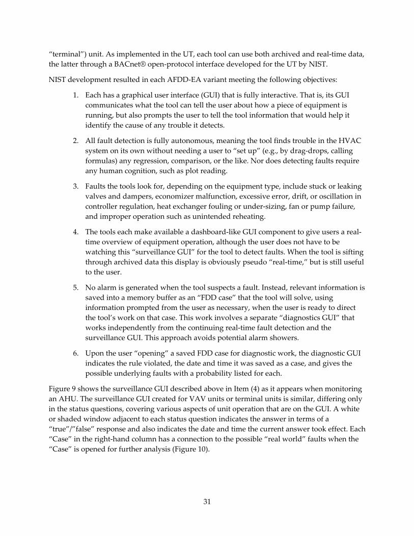
31

“terminal”) unit. As implemented in the UT, each tool can use both archived and real‐time data,

the latter through a BACnet® open‐protocol interface developed for the UT by NIST.

NIST development resulted in each AFDD‐EA variant meeting the following objectives:

1. Each has a graphical user interface (GUI) that is fully interactive. That is, its GUI

communicates what the tool can tell the user about how a piece of equipment is

running, but also prompts the user to tell the tool information that would help it

identify the cause of any trouble it detects.

2. All fault detection is fully autonomous, meaning the tool finds trouble in the HVAC

system on its own without needing a user to “set up” (e.g., by drag‐drops, calling

formulas) any regression, comparison, or the like. Nor does detecting faults require

any human cognition, such as plot reading.

3. Faults the tools look for, depending on the equipment type, include stuck or leaking

valves and dampers, economizer malfunction, excessive error, drift, or oscillation in

controller regulation, heat exchanger fouling or under‐sizing, fan or pump failure,

and improper operation such as unintended reheating.

4. The tools each make available a dashboard‐like GUI component to give users a real‐

time overview of equipment operation, although the user does not have to be

watching this “surveillance GUI” for the tool to detect faults. When the tool is sifting

through archived data this display is obviously pseudo “real‐time,” but is still useful

to the user.

5. No alarm is generated when the tool suspects a fault. Instead, relevant information is

saved into a memory buffer as an “FDD case” that the tool will solve, using

information prompted from the user as necessary, when the user is ready to direct

the tool’s work on that case. This work involves a separate “diagnostics GUI” that

works independently from the continuing real‐time fault detection and the

surveillance GUI. This approach avoids potential alarm showers.

6. Upon the user “opening” a saved FDD case for diagnostic work, the diagnostic GUI

indicates the rule violated, the date and time it was saved as a case, and gives the

possible underlying faults with a probability listed for each.

Figure 9 shows the surveillance GUI described above in Item (4) as it appears when monitoring

an AHU. The surveillance GUI created for VAV units or terminal units is similar, differing only

in the status questions, covering various aspects of unit operation that are on the GUI. A white

or shaded window adjacent to each status question indicates the answer in terms of a

“true”/”false” response and also indicates the date and time the current answer took effect. Each

“Case” in the right‐hand column has a connection to the possible “real world” faults when the

“Case” is opened for further analysis (Figure 10).

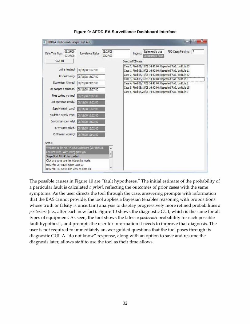
32

Figure 9: AFDD-EA Surveillance Dashboard Interface

The possible causes in Figure 10 are “fault hypotheses.” The initial estimate of the probability of

a particular fault is calculated a priori, reflecting the outcomes of prior cases with the same

symptoms. As the user directs the tool through the case, answering prompts with information

that the BAS cannot provide, the tool applies a Bayesian (enables reasoning with propositions

whose truth or falsity is uncertain) analysis to display progressively more refined probabilities a

posteriori (i.e., after each new fact). Figure 10 shows the diagnostic GUI, which is the same for all

types of equipment. As seen, the tool shows the latest a posteriori probability for each possible

fault hypothesis, and prompts the user for information it needs to improve that diagnosis. The

user is not required to immediately answer guided questions that the tool poses through its

diagnostic GUI. A “do not know” response, along with an option to save and resume the

diagnosis later, allows staff to use the tool as their time allows.

33

Figure 10: AFDD-EA Diagnostic Interface

All the interactive capabilities just described are achieved because the AFDD‐EA tools are

“expert systems”, as explained in the following paragraphs.

3.2.2 Expert System Techniques in the UT AFDD Module

Expert systems are computer programs that replicate or enhance the reasoning and judgment

that humans, having expertise in a specific field, exercise on data requiring evaluation and

action from their expertise. Expert systems obviously do not replace human expertise, but

instead extend it to applications where it would not be physically or economically feasible

otherwise. Expert systems are generally distinguished from other forms of artificial intelligence

by their having two core components: a knowledge base and an inference engine.

A key characteristic of AFDD‐EA compared to earlier FDD work by NIST is its automating and

assisting parts of the fault diagnosis (as contrasted to detection) effort that previously fell totally

upon the user. Where both APAR and VPACC offered the user only a paper matrix associating

failed rules to possible causes, the AFDD‐EA diagnostic GUI interactively steps the user

through a probability‐driven case solution process, employing techniques from the area of

artificial intelligence known as expert systems. This enables a novel potential for HVAC FDD to

efficiently resolve rule infractions where external mitigating factors can exist, or where the

evidence is uncertain or even contradictory. In the current AFDD‐EA, this potential is exploited

relatively modestly, by presenting the user with fault hypotheses, updating their a posteriori

probabilities as diagnosis proceeds, and then “learning” the final, verified case solution to

provide better a priori probabilities later.

34

3.2.3 Knowledge Base and Inference Engine

In AFDD‐EA, the knowledge base includes the elements a human HVAC expert considers when

reviewing data acquired from equipment: operating expectations (i.e., rules), hypotheses of

what could be wrong if any rule is not met, and the evidence needed to figure out which

hypothesis is the true one. A simple machine learning technique, the Bayes classifier, is the

inference engine that AFDD‐EA currently uses to assign to each hypothesis a relative

probability that it is the one behind a given rule infraction. Machine learning techniques are

those that “learn from experience” as various faults are encountered and solved over time.

3.2.4 Rules and States

Like APAR, AFDD‐EA uses “rules” as its basis for detecting faults. A rule is an expression in

program code testing the data fed into the tool for specific characteristics. In AFDD‐EA, rules

are written as pairs of if‐then statements in binary (i.e., valued either “true” or “false”) logic. For

any “if” expression that is true, a complementary “then” expression must concurrently also be

true for the equipment to be regarded as operating satisfactorily. A false “then” resulting from a

rule’s true “if” does not cause an alarm immediately, but instead falls into a circular buffer as an

event violating that rule. Over an adjustable period of sampling time (e.g., one day) the rule

violated most frequently is identified and a FDD case about it is (as described earlier) created

and saved to memory for later diagnosis. That rule is then blocked from creating more cases

until the stored case is solved, verified, and learned via the diagnostic GUI.

“States”, rather than the numerical data themselves, are the terms used in rules. As each

numerical value—for example, “Tair, supply”, sampled from a supply air temperature sensor—

is passed into the tool, one of the states it generates by a control chart analysis of the stream of

“Tair, supply” values is a binary logical state, such as “supply AirTempInBand”. This state is

valued “true” when the temperature is regulated within the band allowed and “false” when it is

not.

States and rules together form a flexible infrastructure with which to automate the detection

and diagnosis of faults. Very sophisticated inferences can be programmed as chains of states

and rules, with branching used to create the complex reasoning known in artificial intelligence

as a “production” (meaning reasoning, like that of a human expert, is produced). AFDD‐EA is

an innovative first step in this direction, which NIST will more fully develop with experience in

the future.

3.2.5 Fault Case Management

Through the diagnostic GUI, the user can see a listing of the FDD cases a piece of equipment has

pending, and can address each as time permits. Cases can be partly worked through, saved and

closed away to attend to some other matter, and then reopened later. New cases similar to

existing ones are blocked to avoid redundancy. Real‐time surveillance for new faults is

unaffected by the diagnostic process. Commissioning agents in particular have voiced to NIST

that FDD tools should give them a way to manage the plethora of faults they routinely face

when starting HVAC systems up. The innovative “case management” within AFDD‐EA

provides such a way, bringing to the tool an unprecedented degree of user–friendly

interactivity.

35

3.2.6 Control Loop Diagnostics 3.2.6.1 User interface for the control loop diagnostic module and sample testing results

A simple UI was developed in UT3 for this diagnostic module and is shown in Figure 11. There

are two methods for setting the set‐point in this analysis module. As a default, users will select

the data folder, testing channels for the set‐point, and measured variable and control signals. If

the set‐point is known to be constant during operation, users can also check the checkbox for

“Use Constant Set‐point” and specify a constant value for the set‐point.

Figure 11: User Interface for Control Loop Diagnostic Module

Users can also select a loop oscillation period and diagnostic sensitivity. Fast loops would have

an oscillation period of less than 3 minutes if they were to oscillate, medium loops between 3

and 30 minutes, and slow loops greater than 30 minutes. The diagnostic threshold is defined

relative to the noise level. For high sensitivity, the threshold is set at 3 times the noise level,

medium sensitivity at 6 times the noise level, and low sensitivity 10 times the noise level.

Importantly, users need to adjust the data sampling interval for testing control loop hunting

(Figure 12). The default time interval in the Channel Folder is 15 minutes. If the data time

interval is not appropriate for testing, a warning message is issued, as shown in Figure 13. For a

slow loop, a data sampling interval of no more than 10 min should be used, if possible; for a

medium speed loop, a data sampling interval of no more than 1 min should be used, if possible;

for a fast loop, a data sampling interval of no more than 6 sec should be used, if possible.

36

Figure 12: Window for Channel Folder Properties

Figure 13: User Interface with Warning Message on Time Interval of Data Channels

The analysis is performed for the time periods where the data meet the testing criterion that the

set‐point should be approximately constant. The diagnosis results are reported on completion of

the analysis. A sample report, including tested channels and diagnostic results, is shown in

Figure 14. Trend data plots (Figure 15) for the period with the most severe control loop hunting

are generated.

37

Figure 14: Diagnostic Report from Control Loop Diagnostic Module

Figure 15: Trend Data Plot for Set-Point, Measurement, and Control Signals from Control Loop Diagnostic Module

38


Project 4 resulted in a number of accomplishments that involved both model and test procedure

validation, as well as implementation of related analyses in the UT, and dissemination of

related information:

1. Validation of the LBNL fan efficiency and speed models in EnergyPlus, and

implementation of related analyses in the UT.

2. Validation of the LBNL system curve model in EnergyPlus, and implementation of

related analyses in the UT.

3. Implementation of analyses in the UT to determine coefficients for the simple VAV fan

model in EnergyPlus.

4. Validation of the VFD efficiency model in EnergyPlus.

5. Creation of a fan system test facility at LBNL to support further research on fan system

component performance.

6. Validation of Modera’s air leakage test procedure.

The following provides further detail about each of these six accomplishments.

3.3.1 Fan Efficiency and Speed Models

As described in the EnergyPlus Engineering Reference (U.S. DOE 2013), the LBNL fan efficiency

and speed models had been developed using data from only eight different fans. To assess

whether the models can be applied over a broader range, sets of fan static pressure, flow, shaft

power, and speed data for an additional 29 fans were generated using manufacturer’s

published performance maps, a commercial graphic digitizing program (DigitizeIt), and an

Excel spreadsheet that was set up to perform least squares fits to the data. The fans included a

variety of centrifugal, axial, and mixed flow fans and included both housed and plenum types.

Maximum power for the fans covered a wide range from 7.5 to 600 hp.

Based on the model coefficients determined for each fan (Miller 2010), the overall average root‐

mean‐square (RMS) difference between predicted and “actual” fan efficiency was 0.7 percent

and the maximum was 1.1 percent. The average RMS difference between predicted and actual

fan power (where the difference is divided by the corresponding maximum power) was 0.9

percent and the maximum was 2.1 percent. For the fan shaft speed model, the average RMS

percent difference between predicted and actual speed was 0.5 percent and the maximum was

0.8 percent. These values represent very good agreement between predicted and “actual”

values.

Subsequently, an analysis module was added to the UT to determine coefficients for the fan

efficiency and speed models. The module is split into two sub‐modules. The first sub‐module

uses fan shaft power, flow, and fan static pressure data loaded into the UT as individual

channels (determined either from field tests or more likely using digitized data obtained from a

manufacturer’s performance map, cast in the form of time‐series data with a sequential artificial

time corresponding to each data point), along with user specification of the fan wheel outer

diameter in the “Settings” window. It uses a non‐linear least‐squares (LSQ) method developed

at Argonne National Laboratory (More 1977, More et al. 1980) and an implementation of the

39

mathematical error function erf (Geelen 1993) to calculate coefficients for the fan efficiency

model in both normal and stall operating regions (normalized Eu less than and greater than

zero, respectively). The sub‐module also reports various data statistics, which include:

the maximum Eu value for normalizing the data (corresponds to maximum efficiency),

normalized Eu values that correspond to maximum efficiency less 10 percent (bounds

recommended for fan selection, ASHRAE 2012), and

the normalized Eu values that correspond to 10 percent efficiency (fan operation beyond

these limits means that more than ten times more power is required to drive the fan than

air power produced, and represents unlikely operation).

The latter criterion is used to bound the region over which output data fit statistics are reported.

Those statistics include average, RMS, minimum, and maximum errors in predicted fan power

(percent, fit/maximum power) separated into normal and stall operating regions. In addition,

the sub‐module generates three charts: 1) a “pressure rise versus flow” chart in the same format

as a manufacturer’s performance map for visual verification that fan power “curves” entered

for analysis are as intended; 2) a “normalized efficiency” chart, which shows the data translated

into dimensionless form as normalized efficiency (efficiency divided by maximum efficiency)

versus the corresponding normalized Eu values; and 3) a “fan power error” chart, which shows

the differences between predicted and data channel fan power, separated into normal and stall

operating regions. Figure 16 shows examples of these three charts for one fan.

Figure 16: Example Chart Output from UT Fan Efficiency Sub-Module

40

The UT module also includes a similar sub‐module for fan speed analysis after the fan efficiency

analysis is complete. This second sub‐module uses similar data, but fan shaft speed is used

instead of power. To maintain proper scaling in the dimensionless parameter space (normalized

Eu coordinate system), the user must enter as “settings” the maximum Eu as well as the

normalized Eu values corresponding to 10 percent efficiency in the normal and stall operating

regions that were reported by the efficiency sub‐module. In the future, capabilities should be

added to the UT API so that these values can be automatically transferred between analysis sub‐

modules (and so that the user can select the efficiency limits of interest). The same LSQ method

used for efficiency analyses is used to determine the speed coefficients. Like the efficiency sub‐

module, the speed sub‐module also reports similar data statistics and generates charts. Figure

17 shows examples of the three speed‐related charts for the fan shown in Figure 16.

Figure 17: Example Chart Output from UT Fan Speed Sub-Module

3.3.2 System Curve and Simple VAV Fan Models

The Sherman and Wray (2010) system curve model was validated using fan static pressure and

flow data collected from two VAV air‐handlers operating on one floor over several weeks in a

25‐story large office building in Sacramento, CA (Grahovac 2010). Each air‐handler is a draw‐

through packaged unit equipped with an outdoor and return air mixing chamber, a filter

section, hot‐water preheat and chilled‐water coils, and a backward‐curved centrifugal plenum

fan driven by a belt, electric motor, and VFD. The duct system connected to these air‐handlers is

comprised of a loop with 38 VAV boxes, and a single duct static pressure sensor is located at the

farthest point in the loop from the air‐handlers. Duct static pressure at this point is controlled to

1.0 inch water column (249 Pascal). Fits to the pressure rise and flow data for a fixed outdoor

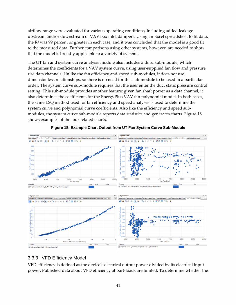
41

airflow range were evaluated for various operating conditions, including added leakage

upstream and/or downstream of VAV box inlet dampers. Using an Excel spreadsheet to fit data,

the R2 was 99 percent or greater in each case, and it was concluded that the model is a good fit

to the measured data. Further comparisons using other systems, however, are needed to show

that the model is broadly applicable to a variety of systems.

The UT fan and system curve analysis module also includes a third sub‐module, which

determines the coefficients for a VAV system curve, using user‐supplied fan flow and pressure

rise data channels. Unlike the fan efficiency and speed sub‐modules, it does not use

dimensionless relationships, so there is no need for this sub‐module to be used in a particular

order. The system curve sub‐module requires that the user enter the duct static pressure control

setting. This sub‐module provides another feature: given fan shaft power as a data channel, it

also determines the coefficients for the EnergyPlus VAV fan polynomial model. In both cases,

the same LSQ method used for fan efficiency and speed analyses is used to determine the

system curve and polynomial curve coefficients. Also like the efficiency and speed sub‐

modules, the system curve sub‐module reports data statistics and generates charts. Figure 18

shows examples of the four related charts.

Figure 18: Example Chart Output from UT Fan System Curve Sub-Module

3.3.3 VFD Efficiency Model

VFD efficiency is defined as the device’s electrical output power divided by its electrical input

power. Published data about VFD efficiency at part‐loads are limited. To determine whether the

42

LBNL VFD efficiency model in EnergyPlus could be applied broadly to predict VFD efficiency

for HVAC applications in large commercial buildings, performance data were collected directly

from manufacturers (Krukowski and Wray 2013). Of the 22 manufacturers contacted, only five

could provide part‐load data and even some of these data were too limited to be of use. In the

end, 44 models from three manufacturers were analyzed. The drives were rated over a wide

range between 1 hp and 200 hp. The average RMS error in using the model to predict

manufacturer’s efficiency for each VFD analyzed was 0.25 percent while the maximum RMS

error was 0.90 percent. The average maximum difference between fitted and manufacturer

efficiencies was 0.54 percent. The low RMS errors demonstrate that the VFD efficiency model is

suitable for the data provided by the manufacturers.

It is important to note that the collected data sets were generated in the absence of test

standards. In December 2011, American National Standards Institute (ANSI)/AHRI Standard

1210, “Performance Rating of Variable Frequency Drives” was published. It specifies methods

for measuring the “performance” of VFDs used in HVAC applications. Drives evaluated

according to the standard will have published ratings for drive system efficiency at various

speeds and loads. In particular, the standard requires that the VFD be connected to a motor

during tests because the reported efficiency is the ratio of motor mechanical output power

divided by VFD electrical input power, which is not VFD efficiency. As a result, to use the 1210

test results during system design, one still needs to know whether the intended combination of

VFD and motor matches the 1210 test configuration. Once data collected using this standard

become available, methods should be developed to separate out the VFD and motor efficiencies

and the 44 drives that the team analyzed should be reevaluated to verify whether the LBNL

model still holds, or the equation should be reformulated to represent VFD and motor

packages. Because of the uncertainty at this time regarding VFD and motor efficiency data, a

related UT analysis sub‐module was not produced.

3.3.4 LBNL Fan System Test Facility

A test facility for assessing fan system performance was created at LBNL, using one of the three

main fans serving a constant‐volume reheat supply air system in Building 90. The fan is a

forward‐curved single‐wheel‐double‐inlet centrifugal fan driven using three V‐belts by a

nominal 30 hp three‐phase electric motor. The motor is connected to a VFD, which provides the

capability to vary fan speed as needed. A damper in the discharge duct provides a means to

alter flow resistance downstream of the fan. The fan inlet is unducted and air is drawn from a

plenum room located downstream of associated heating and cooling coils. To measure fan flow

continuously, a custom multi‐tube multi‐point pressure averaging grid set (one set of five tubes

with 25 points senses upstream total pressure, the other set of three tubes with 15 points senses

roughly the maximum negative static pressure) was constructed and installed downstream of

the fan, and calibrated using tracer gas. Fan pressure rise is measured using static probes

located in the fan room and in the discharge duct just downstream of the fan. Pressures are

measured using an Energy Conservatory multichannel auto zeroing pressure transducer. Fan

shaft and motor shaft torques and speeds (product of these parameters for each component is

shaft power) are measured using custom‐built Sensor Development Inc. pulleys with strain

gauges attached to their hubs and optical speed encoders at the shaft ends. These parameters, as

43

well as VFD output power as reported by the VFD itself, are logged through multiple

standalone data acquisition systems. Our intent in setting up this system is to support the

development of field diagnostic procedures for determining VFD, motor, belt, and fan

efficiencies as a function of flow and pressure rise, as well as a function of VFD settings and belt

alignment and tension.

Because almost no data are available about belt efficiency, initial experiments were performed

to assess whether there is a significant correlation between belt efficiency and belt temperature,

as measured on the belt outer surfaces just after the belt exited the motor pulley (before it

approaches the fan where increased flow could cool the belt), using a non‐contact close‐focus

infrared thermometer. Unfortunately, it was found that these belt temperatures did not change

significantly even though belt efficiency decreased from about 90 percent at full speed to about

20 percent at 25 percent speed. This was an unexpected result, because the power lost due to the

belt inefficiency (and thus the belt heat input) decreased substantially as the speed dropped:

from about 2 kW at full speed to about 0.6 kW at 25 percent speed, and one would expect belt

temperature to vary as a result. Further work is needed to determine whether other temperature

measurement locations (e.g., the belt inside surfaces or motor pulley grooves) could yield useful

results. At the suggestion of one our industry participants (Lau Fans), another possible future

direction is to instead assess whether belt slip (motor speed versus fan speed, taking into

account the drive ratio between motor and fan pulleys) could be correlated with efficiency.

Due to difficulties encountered in setting up the shaft power measurement system (likely

caused by ground loops between sensor components and the data acquisition system), the team

was unable within the project’s resources to collect simultaneous data that allow us to calculate

fan efficiency itself. Future work should do so. Also, although other staff had “calibrated” the

VFD output power signals, it was found that the reported VFD power output was less than the

motor shaft power, which cannot be correct. As a result, no further electrical measurements

were made, and future work needs to include using elaborate electric power meters that have

sufficient bandwidth to measure VFD output power (as well as VFD input power).

3.3.5 Modera’s Leakage Test Procedure

Air‐handling system leakage reduces the amount of air delivered to conditioned spaces and in

most cases wastes energy and money. Standards exist for where and how to measure system air

tightness, but they tend to focus on new construction, and only on the high‐ and medium‐

pressure portions of the system. Modera et al. (2013) investigated air leakage in the “low‐

pressure” portions of a large commercial‐building air‐handling system (i.e., downstream of

variable‐air‐volume box inlet dampers) using a simplified diagnostic protocol for measuring

low‐pressure leakage that can be used during normal system operation in an existing building

(Modera 2007).

In particular, the protocol was tested using the duct system as found and with a calibrated leak

added. The test results indicate that normalized leakage (airtightness) can be measured to

within 10 liters per second at 25 Pa, with and without the existence of significant flow through

the minimum opening of the box inlet damper. Field test results from nine other buildings

indicate that “low‐pressure” leakage varies considerably from system to system (standard

44

deviation of 50 percent of the mean value). The average value corresponded to approximately

10 percent of the flow entering the low‐pressure system sections. The variability of the

measured results, combined with a simplified analysis of the impacts of this leakage, suggest

that testing low‐pressure system leakage in commercial buildings should be economically

justifiable. Although the test requires analyses, it does not involve collecting time series data, so

a related analysis module was not added to the UT. A calculation tool (e.g., in the form of a

mobile phone application) should be developed to facilitate use of Modera’s test protocol.


The development of the new version of the Universal Translator (UT3) for this project consisted

of two interrelated components. They are the UI and the API. The UI design focused on the

needs of the end user for UT3, while the design of the API focused on the developers.

3.4.1 User Interface

When starting the UI design of UT3, the development team looked at feedback from UT2 users

as well as support issues. Several key issues became apparent. The primary issue with regard to

the UI was that UT2 was too complicated. To reduce the complexity of UT3, the UI is organized

to follow a logical work flow used by the engineers as they process data. The general data

processing steps are to import data sources, organize data into logical groupings, filter the data,

visualize the data, and finally perform various analyses on the data. The UT3 UI follows this

same approach. Each section of the UI will be briefly described below.

Two additional issues with UT2 were the low speed and trouble associated with importing files.

Making UT3 as fast and stable as possible became the next highest priority design goal. Along

with the speed, UT3 needed to handle larger data sets. An alpha version of UT3 was created

using requirements developed from the above feedback.

The feedback from TAG members came after the alpha version of UT3 was released. TAG

members liked the new functionality of UT3, commenting that they wanted to see additional

features with respect to importing data. Adding the ability to append new data to existing data

sources was a primary request that would speed up the process of doing monthly analysis.

Adding data to existing UT3 projects would eliminate the need to start from scratch each month.

The UT3 UI was changed to accommodate this request and a beta version of UT3 was released.

Some of the more popular feature requests are listed in Chapter 5. Additional information about

the TAG’s reaction to the UT3 UI can be viewed at http://utonline.org/cms/. All TAG meetings

have been recorded and notes have been posted.

The main project navigation tool is located in the upper left hand corner of the UI and is labeled

“Project View” (Figure 19). The navigation tree is laid out in a sequential order. The order

follows the typical process of gathering, organizing, processing, visualizing, and then analyzing

data. Figure 20 shows the project view layout.

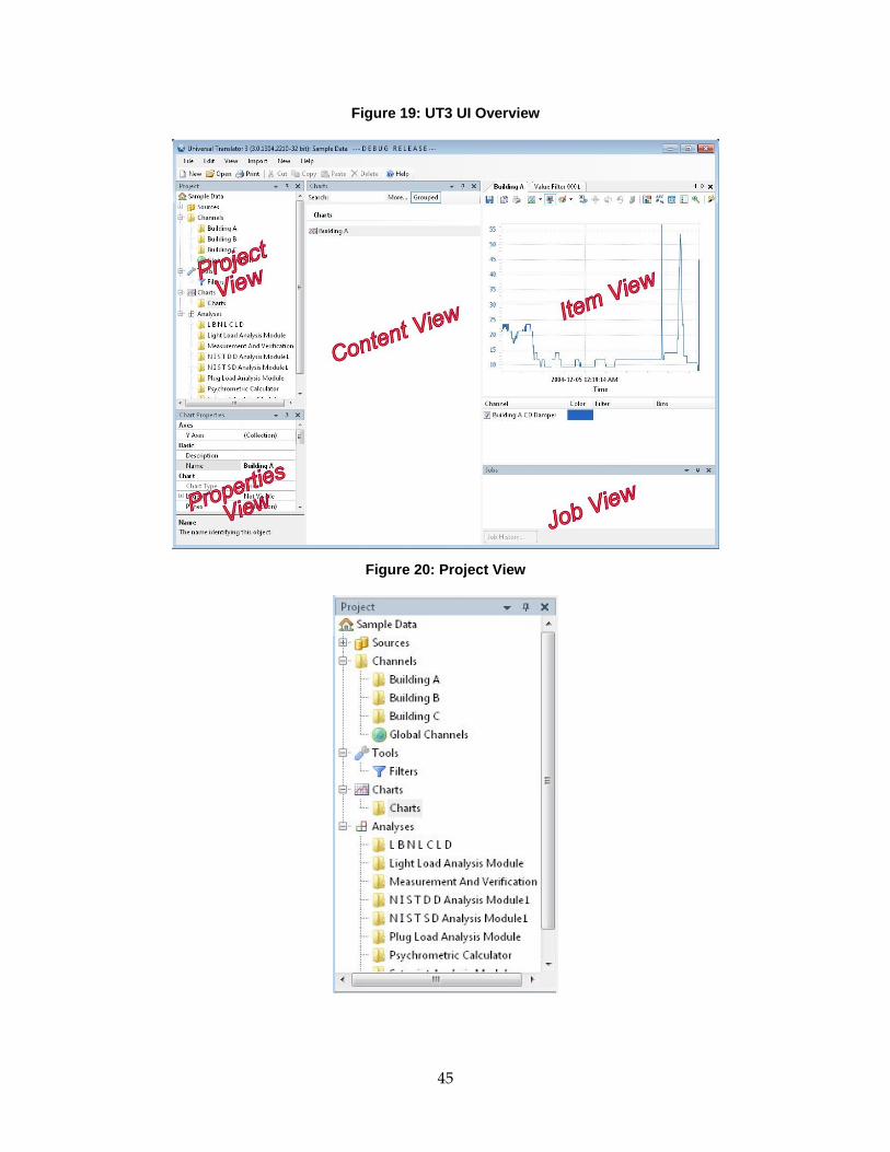
45

Figure 19: UT3 UI Overview

Figure 20: Project View

46

3.4.1.1 Data Source Node

The first node contains the raw data sources. The data source could be anything from text files

to databases to BACnet (a communications protocol for building automation and control

networks that is an ASHRAE, ANSI, and ISO standard protocol) enabled control systems. As

new data sources are added to a UT3 project, they will be displayed under the Source node. The

data sources may be edited in the “Source” node.

After data are added, the next task is to define the project channels (e.g., raw data that have

been synchronized with each other, or synthesized “pseudo” data). The project channels are

created and displayed in the “Channels” node of the navigation tree. The project channels can

reference a single data channel or they can be defined as any number of pseudo channels. The

pseudo channels include a constant value channel, psychrometric channel, or formula channel.

The value of a pseudo channel is calculated during the resampling process. Channels are

automatically created for each data source as they are added to the data source section.

3.4.1.2 Data Channel Node

The project view is also used to organize the data channels into folders. Figure 21 shows an

example of data organized into channels. Organizing channels into folders is necessary for some

analysis routines. Folders are also useful for organizing a group of channels for export to a

comma separated value file.

Figure 21: Sample Data Organized in Channels Node

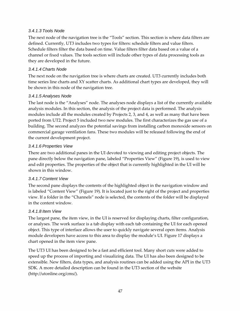
47

3.4.1.3 Tools Node

The next node of the navigation tree is the “Tools” section. This section is where data filters are

defined. Currently, UT3 includes two types for filters: schedule filters and value filters.

Schedule filters filter the data based on time. Value filters filter data based on a value of a

channel or fixed values. The tools section will include other types of data processing tools as

they are developed in the future.

3.4.1.4 Charts Node

The next node on the navigation tree is where charts are created. UT3 currently includes both

time series line charts and XY scatter charts. As additional chart types are developed, they will

be shown in this node of the navigation tree.

3.4.1.5 Analyses Node

The last node is the “Analyses” node. The analyses node displays a list of the currently available

analysis modules. In this section, the analysis of the project data is performed. The analysis

modules include all the modules created by Projects 2, 3, and 4, as well as many that have been

ported from UT2. Project 5 included two new modules. The first characterizes the gas use of a

building. The second analyzes the potential savings from installing carbon monoxide sensors on

commercial garage ventilation fans. These two modules will be released following the end of

the current development project.

3.4.1.6 Properties View

There are two additional panes in the UI devoted to viewing and editing project objects. The

pane directly below the navigation pane, labeled “Properties View” (Figure 19), is used to view

and edit properties. The properties of the object that is currently highlighted in the UI will be

shown in this window.

3.4.1.7 Content View

The second pane displays the contents of the highlighted object in the navigation window and

is labeled “Content View” (Figure 19). It is located just to the right of the project and properties

view. If a folder in the “Channels” node is selected, the contents of the folder will be displayed

in the content window.

3.4.1.8 Item View

The largest pane, the item view, in the UI is reserved for displaying charts, filter configuration,

or analyses. The work surface is a tab display with each tab containing the UI for each opened

object. This type of interface allows the user to quickly navigate several open items. Analysis

module developers have access to this area to display the module’s UI. Figure 17 displays a

chart opened in the item view pane.

The UT3 UI has been designed to be a fast and efficient tool. Many short cuts were added to

speed up the process of importing and visualizing data. The UI has also been designed to be

extensible. New filters, data types, and analysis routines can be added using the API in the UT3

SDK. A more detailed description can be found in the UT3 section of the website

(http://utonline.org/cms/).

48

3.4.2 API/SDK Development

The second part of Project 5 was the development of the SDK. The UT3 SDK is used both by

third party developers and by the UT3 development team. The UT3 UI is written on top of the

SDK. All of the data adaptors and filters included in the UT were also written using the SDK.

There are two possible approaches to the UI and the integration of third party add‐ins in

general. The first is to create a tool kit that the authors of the analysis module use to create their

own interfaces. The second and the one chosen for this project, is to have a unified UI with

hooks to allow the analysis module author to add their module into the UT3 UI. Having a

unified UI makes the user experience easier, allowing the user to learn one UI for all the basic

functionality. This approach also reduces the amount of UI that the analysis creator has to write.

Microsoft’s Visual Studio 8 with the .NET 3.5 framework was chosen to develop UT3’s UI and

SDK. C# was chosen as the programming language and any .NET compatible programming

language could be used to develop the UT extension. This platform was chosen because of the

large number of developers proficient in this platform.

The SDK enables third party developers to extend the functionality of the UT in several areas.

These areas include filters, data import adaptors, and analysis modules. Having these areas

extensible allows the UT development team and third party developers the ability to enhance

the functionality without having access to the core source code. Deployment of new extensions

is also possible without having to install a new version of UT3.

UT3 does not use a database for data storage. Instead, UT3 uses a file‐based serialization engine,

because of the need to process data rapidly. During the early stages of development, the

development team ran performance tests for a number of popular databases. None of them

were even remotely close to being as fast as a file‐based system. A secondary benefit to this type

of system is that there is no need to install a supporting database engine. Also, transferring

projects from one computer to another is as easy as copying a folder from one computer to

another. Creating a backup of the project folder is also an easy way to back up a project.

The UT3 SDK includes a few sample projects, a programmer’s guide with an API reference,

Visual Studio project templates for creating UT3 extensions, and the UT3 application. Several

how‐to tutorials are also available on the UT website (http://utonline.org/cms/).

The API consists of an extensive set of .NET objects. The objects consist of data processing

objects and well as UI helper objects. The analysis module extension is simply a UT3 object that

the developer inherits. Deployment of a new analysis module is as simple as copying a

directory of files to the UT extensions directory on the user’s computer. Figure 22 gives an

overview of the UT3 program layers.

49

Figure 22: High Level Overview

The UT3 Application consists of the following components:

The application executable (define), containing the application UI and logic to execute

commands invoked by the user.

Plug‐ins: dynamically loaded libraries and objects. Plug‐ins can be written by anyone

with access to the UT3 SDK. Plug‐ins are one of two types:

o Data Adapters, objects that enable the user to import data from specific data

sources.

o Analysis Modules, objects that enable the user to analyze imported data.

Both the application executable and plug‐ins use the UT3 SDK as a base. The UT3 SDK contains

the following:

UI components used by the UT3 application and plug‐ins.

The Data Adapter API, a sub‐set of the UT3 SDK specifically for Data Adapter

developers.

The Analysis Module API, a sub‐set of the UT3 SDK specifically for Analysis Module

developers. Included in the Analysis Module API:

o The ability to create and modify charts and reports within an Analysis Module.

o A matrix library for linear algebra calculations, such as linear regressions.

Tools for processing data, including data point collections, time‐conversions, and data

filtering.

Code enabling the UT3 application to save and restore all data structures in a UT3

project file, called “Persistence” in the diagram.

50

To assist users, several tutorials have been included in the SDK, but the inclusion of sample

projects has proven to be most effective.

3.4.3 Additional Applications

Several new analysis modules were developed and included in UT3:

3.4.3.1 Lighting Load

The Light Load analysis module considers the availability of control devices for light loads and

calculates the potential savings using that technology.

3.4.3.2 Plug Load

The Plug Load analysis module considers the availability of control devices for plug loads and calculates the potential savings using that technology. For most plug load types, the analysis is based upon occupancy data for the space and power or amperage data of the load prior to a retrofit. For some loads, the Plug Load Analysis Module can calculate the potential savings based on typical duty cycles and the measured savings from actual retrofits. This analysis module will provide the potential energy savings for an occupancy type plug load controller.

3.4.3.3 Psychrometric Calculator

The Psychrometric Calculator analysis module calculates moist air properties on the basis of a

psychometric property table.

The following inputs are required to calculate properties:

Barometric pressure

Dry bulb temperature

A measure of humidity:

o Wet bulb temperature, or

o Dew point temperature, or

o Relative humidity, or

o Humidity ratio.

3.4.3.4 Setpoint

The Setpoint analysis module performs a statistical analysis on trend data and displays the

results in a table. It will display “Percent of Time Over Upper Setpoint” and “Percent of Time

Under Lower Setpoint”, Minimum and Maximum values, as well as averages and actual times

over or under set‐point.

3.4.3.5 Statistics

This Statistics analysis module will calculate statistics for selected trends.

3.4.4 UT Website

The UT website (http://utonline.org/cms/) includes a set of UT3 training videos and also enables

users to submit bug reports and feature requests

51

CHAPTER 4: Project Outcomes


4.1.1 Outcomes

The overall Program goal to develop analysis modules within the UT framework was achieved

for the M&V tool. The UT’s data upload, merging, and time‐interval re‐sampling functions have

been demonstrated to streamline the arduous exercise in data preparation usually required in

M&V analysis.

Complex regression modeling functionality has been programmed into the M&V analysis

module. Regression models using time as well as an independent variable, usually ambient

temperature, have been included in the Tool. The user may use menu‐driven selections to

customize modeling types and apply them to filtered sets of data. This allows users to think

more about how to model a building properly rather than about the mechanics of the regression

process. Various charts and graphs allow the users to quickly assess model fit and performance

in the development of appropriate models.

The ability of the M&V tool to set up analysis bins based on filtering the data in different time

periods is useful to improve modeling accuracy. Occupied and unoccupied periods exhibit very

different energy use behavior. One tool tester asserted that the tool should allow for automatic

filtering of the data, as well as allowing the tool to set up a function to vary the start‐stop

operation in a building, as many buildings operate in this way. Although such features may be

useful, they are beyond the scope of the current project. It was noted, however, that the users

have begun to think about useful tool features that would make it more generally applicable.

The tool‐testing group reported satisfaction with the UT3 M&V analysis module and with the

tutorial that walked them through the process. Many from the testing group were favorably

impressed by the UT’s computational speed and features.

Regarding the M&V analysis module, the decision to use a time‐and‐temperature based model

rather than simple change point models was advantageous. Testing group members liked the

accuracy the tool provides when using hourly time intervals, allowing them to visualize times

throughout the day or week when savings are being achieved. This aspect of visualizing

projected baseline usage along with measured post‐installation usage is helpful to owners and

service providers to maintain savings over time.

Tool users also noted that the time‐and‐temperature model, which was developed by LBNL, has

applications in demand response. Using 15‐minute or hourly analysis time intervals, baseline

models can be developed and used to estimate demand reductions when a utility calls a

demand reduction event. While the M&V tool was not developed specifically for quantifying

these benefits, the principles are the same. It is noted that future tool developments could

include demand response applications.

52

Overall, the M&V tool provides users with a means to develop a rigorous M&V analysis in a

streamlined process. It provides advanced regression modeling capability, and allows users to

test multiple scenarios to get the best energy models. It also enables users to focus on the M&V

approach and uncertainties in baseline modeling and savings at key points in an energy

efficiency project, rather than on the actual analysis required to prepare data.

A few key elements of the project could have had better outcomes. For example, the M&V tool

testing group only had a few active participants. Although access to the website with software,

data, and a tutorial were available, and a forum for receiving comments was provided, no active

discussions were started beyond a few comments. While the few comments were helpful and

informative, more feedback from the user community would have been beneficial. In retrospect,

this could have obtained by a wider solicitation of potential testers, e.g., through publicity at

industry meetings and in trade journals. To this end, the team collected useful feedback during

presentations of the tool to specific users in webinars and meetings. This feedback continues

through emails and informal discussions. It is expected that additional feedback will be

obtained now that the tool is generally available as part of UT3 and more users are beginning to

apply the M&V module. Incorporating that feedback and suggestions for tool improvement will

need to be funded by future sources.

There was a significant lack of data sets for M&V tool testing. Building owner data are

proprietary, and multiple data sets are needed to test the tool’s algorithms over a wide range of

data sets, baseline and post‐installation periods, and analysis time intervals. Obtaining these

data sets proved to be problematic. A data collection plan identifying sources of data, and

possibly engagement of a formal third party testing contractor may be necessary to provide the

level of testing and validation required.

The early round of testing included a version of the M&V tool without the uncertainty analysis

algorithms. In addition, the uncertainty method’s cross‐validation approach had some

drawbacks in terms of the amount of data required. More testing is required of the uncertainty

algorithm, across a broader set of building data. This feature was not tested or assessed by the

testing group. After the final technical advisory group meeting, several members requested

access to the Tool for the purposes of testing it. Their feedback has not been collected as of this

writing.

4.1.2 Market Impacts

The M&V tool was originally conceived to provide a layer of quality assurance for savings

results in utility energy efficiency programs. Retro‐commissioning (RCx) programs, where

improvements to building system operations are identified and implemented, have been shown

to suffer poor savings performance. There are multiple causes of poor performance: measured

savings are incorrect or overly optimistic, measures are not installed and commissioned

correctly, and measures are removed because they cause problems elsewhere in the system. The

current structure of RCx programs does not afford additional work to verify the savings. These

programs make up a significant part of California investor owned and large municipal utility

program portfolios, and such programs engage many service provider firms. The tool

developed in this project will allow these users to verify savings with minimal costs.

53

The M&V tool has applications in any energy savings project, including traditional audit and

retrofit programs in the residential, commercial, and industrial sectors, but it is not limited to

utility‐run energy efficiency programs. Anywhere there is short‐time interval data for gas,

electricity, or other energy sources, there is the potential for application of the M&V tool. This

includes sub‐metered building systems.

In particular, market actors for the M&V tool will include energy efficiency service providers,

energy service companies, utility program technical reviewers, and utility program evaluators,

each of whom are well versed in energy efficiency analysis. There are many such firms in

California, each with multiple energy efficiency engineers and project managers. In addition,

with the tool’s ability to lower the bar in terms of requiring highly skilled regression analysis

experts, and the increasing availability of Smart Meter data, it is anticipated that new actors will

begin using the tool. These groups may include mechanical, electrical, and controls contractors,

who may be motivated to demonstrate the value of their service to their customers, and

building operations personnel, who are motivated to demonstrate value to their owners. The

M&V tool may become the low‐cost means to demonstrate this value.

Market impacts may also be realized through the development of new program designs.

Currently, the concept of a “Whole Building Approach” to energy efficiency within a building is

gaining traction in California and nationwide. Under these programs, savings are determined

by a whole building M&V process.2 All energy efficiency measures installed in the building are

evaluated together as one package, including major system upgrades or retrofits, operational

improvements, and behavioral programs (such as “lights‐out” programs, or interoffice energy

saving competitions). The M&V tool provides a convenient open‐source means to determine

savings under these programs.

4.1.3 Benefits to California Ratepayers 4.1.3.1 Energy Benefits

The M&V tool provides indirect energy benefits to efficiency projects. Unlike the FDD modules

of Projects 3 and 4, the M&V tool does not help users identify savings opportunities in

individual buildings that when addressed lead directly to savings. The M&V tool, however, can

validate the level of savings actually realized in projects, but this level may be higher or lower

than the savings expected at the outset of the project. M&V helps project participants

understand when projects are not meeting expectations so that corrections may be made. Using

the M&V tool in energy efficiency projects provides a “self‐check” quality assurance function,

and can yield additional savings.

A specific example may be made with utility program RCx projects, enabling programs that

would not otherwise exist. RCx measures identified in these programs serve to improve

building systems’ operational efficiency through implementation of low‐cost measures. Savings

estimates require streams of monitored data and detailed analysis using several assumptions.

2 This process is essentially IPMVP’s Option C Whole Building, or ASHRAE Guideline 14’s Whole

Building pathway.

54

These savings estimates made prior to implementation are often in error, as the measures may

not be fully implemented, assumptions about post‐implementation operations may be

inaccurate, and the measures may be defeated shortly after their implementation. These issues

are well documented in evaluation reports (Tso 2010). RCx programs in 2006‐08 were evaluated

to yield only 63 percent electric and 62 percent gas realization rates across all four of California’s

investor‐owned utility RCx program portfolios. This means that about 134,000 kWh/yr and

5,500 therms/yr of savings were not realized, out of targets of about 361,000 kWh/yr and 14,600

therms/yr.

Utilizing an M&V process within these RCx projects would serve to increase the realization rate

for the portfolio of projects in RCx programs. Project sponsors would be required to collect data

for a longer period after measures are installed, and verify their overall savings claims using

more rigorous M&V methods. Example applications are described in Jump et al. (2007). Since

these verification methods are derived from industry standards, savings claims would be more

accurate and well supported, resulting in higher RCx program realization rates.

4.1.3.2 Non-Energy Benefits

Adding M&V to projects as a quality assurance process, and using the M&V tool to minimize

additional costs is a model that may serve projects and programs beyond those served by RCx

programs. In the private sector, ESCOs may use it to assure owners they are realizing the

expected savings. IPMVP‐adherent M&V implemented through the M&V tool can increase

investments in energy efficiency by raising confidence in savings results across multiple project

and program types.

There are several specific non‐energy benefits for California ratepayers that may be anticipated

through adoption of the M&V tool, in utility projects and programs, as well as in the private

sector. These include:

Lowering costs of energy savings quantification by streamlining the data preparation

functions (merging and re‐sampling time‐series data sets), development of regression‐

based energy models, conducting savings calculations, and estimating savings

uncertainty.

Standardizing savings calculations with IPMVP‐adherent methods. Standardization

lowers administrative costs by establishing consistent calculation procedures and data

requirements.

Raising confidence in energy savings calculations. M&V tool savings calculations are

based on comparisons of energy use measurements before and after energy conservation

measures are installed, rather than on complicated engineering calculations that rely on

non‐energy measurements and assumptions that are difficult to communicate and

understand.

Lowering program administration and evaluation costs through standardization and

portability. The M&V tool is a desktop application and its project files are portable and

may be sent electronically to other interested parties. Due diligence reviewers may open

55

the project work files using the free software and review the data preparation, model

development, and savings calculations performed by others without having to decipher

complicated spreadsheets, data, and assumptions.


4.2.1 Outcomes – Automated Fault Detection and Diagnosis Expert Assistant 4.2.1.1 AFDD–EA Developed to Better Meet Needs of Building Owners and Staffs

Project 3 of the program successfully demonstrated that a novel yet viable HVAC AFDD tool

can be built using expert system techniques and data acquired from the BAS. These data can

either come directly from BAS sensors in real–time (utilizing the BACnet® interface developed

by NIST for AFDD–EA) or as archival “trend logs” supplied to the UT in the same manner as is

done for other UT modules.

The AFDD‐EA–based module for UT is an ambitious step in the FDD of HVAC systems. It is

likely that users will expect more from AFDD‐EA than they expected from prior FDD tools,

because AFDD‐EA attempts many more things, both autonomously for users and interactively

with them. Strong feedback is likely, opining what the tool does and does not do well, and both

cases should be regarded as positive developments along a path to more efficiently managed

commercial buildings.

4.2.1.2 Inputs from Universal Translator Project Team and Automated Fault Detection and Diagnosis Module Technical Advisory Group

NIST hosted three web–enabled teleconference presentations about its work on an AFDD

module for the UT over the span of the project. The first was presented on June 2010 internally

to the UT team, giving an overview of NIST FDD experience and proposing the new concepts

that eventually shaped AFDD‐EA. Once an early demonstration version of AFDD‐EA was

running, NIST hosted two 90‐minute TAG meetings about it, one in May 2011 and the other in

November 2011. Four external participants from industry and a national lab attended the first

FDD TAG, and two more (project engineers from energy consulting businesses) attended the

second TAG. Several internal members and nearly all external invitees attended both meetings.

The responses voiced in the meetings were very positive, but the actionable feedback obtained

was very sparse, coming from three participants who carefully collected some thoughts and

conveyed them by email. Those all addressed usability and GUI features rather than offering

any countervailing view on how the tool actually works, although technical aspects had been

presented. The only negative TAG commentary centered on AFDD‐EA tools being inconsistent

with the “look and feel” established for UT through its user application API. Currently, the

tools access the computer’s operating system directly, rather than as UT commands via the API,

to open their own windows and dialogs outside the UT application frame. Given the extensive

real–time background computation and interactive GUI features this or any similarly featured

FDD tool would need, using the current API alone could not work. Revising the API to serve

AFDD‐EA’s needs would have taken an effort inestimable when the project was proposed, and

that work would have been frustrated by AFDD‐EA itself being a “moving target” under

development.

56

4.2.1.3 Tests on Laboratory and Field Data

The development of AFDD‐EA tools for AHU was initially done using real trend logs obtained

from the Phillip Burton Federal Building, as discussed earlier. These logs include no indications

of naturally occurring or deliberately imposed faults, and no narrative log, so it was not

possible to rate tool performance objectively. Development of the terminal unit tool involved

HVAC laboratory data that was well controlled and documented, but only had a single seasonal

instance of each of several faults imposed. The terminal unit variant of AFDD–EA properly

detected and diagnosed individual faults from that inventory.

4.2.1.4 Peer–reviewed, archival journal article

One of the analytical methods used by all variants of AFDD–EA to detect and diagnose HVAC

controller problems is a technique known as control charting, pioneered in the manufacturing

industry and adapted here for automatic execution on data from building automation systems.

An article describing this development, and the knowledge base architecture AFDD–EA uses to

employ it, has been published in the International Journal of HVAC&R Research.

4.2.2 Outcomes – Control Loop Diagnostic 4.2.2.1 Control Loop Diagnostic module for effective control loop evaluation

The Control Loop Diagnostic (CLD) module in UT3 meets the needs of commissioning

providers and facilities staff for evaluating the performance of control loops based on trend data.

It obviates the need for manual inspection of trend data, which is time consuming and labor‐

intensive. The CLD module automatically identifies two common faults in control loops. Initial

testing of the CLD module was conducted in simulation for various types of control loops

before and after loop tuning. The CLD module was then tested on various data sets from real

buildings and its assessment of the control performance was compared to that of an

experienced commissioning provider.

One limitation of the CLD module is that, whereas it identifies two common performance

problems (hunting and constant offset), it does not diagnose the underlying cause. Hunting

may be caused by improper tuning of the controller or it may be caused by hunting in another

loop. Constant offset may be caused by inadequate equipment capacity or by a wide

proportional band. Diagnosis would require more information and more analysis, which could

be addressed in further work. Another possible future enhancement could come from

implementing the results of an impending ASHRAE research project to develop a methodology

for generating a performance index for control loops, though these results would probably not

be available until 2015.


The experience NIST acquired in the field with earlier FDD tools, plus reports by Ulickey et al.

(2010) and Summers and Hilger (2012) support the view that FDD for HVAC systems needs

novel technical advances such as those introduced by the AFDD‐EA module in UT3. Unlike

earlier FDD tools, which presume much greater degrees of human analytical expertise from

their users, the AFDD‐EA module is intended for use by persons whose analytical talents are

typical for building operators and technicians rather than engineering‐graduate consultants. It

is expected that the AFDD‐EA module will make the benefits of FDD, in general, more

57

economically viable for building owners by reducing the costs they incur using FDD. Based

upon the aforementioned reports, a reduction in the costs to implement FDD is expected to

greatly improve its market acceptance and widen the positive impacts it can provide. Where

current business models for FDD services typically require highly‐trained, and thus costly,

hired consultants to provide the analytics needed, the AFDD‐EA module is a first step toward

making FDD cost‐effective for use by a building ownerʹs maintenance staff alone. The greater

analytical autonomy of the AFDD‐EA module also makes possible comprehensive monitoring

of the thousands of HVAC system components typical of large commercial buildings,

something not economically plausible under any model of FDD services relying upon continual

involvement from human analytical experts.

The CLD module is expected to be used by commissioning providers and trained in‐house

operators and maintenance personnel to enable greater accountability for correct installation

and loop tuning on the part of controls contractors and service technicians. This accountability

will be enabled by the CLD module providing objective evidence of unsatisfactory performance.

The CLD module is also expected to be used by controls contractors and service technicians to

ensure that the performance they are required to provide is delivered to the owner and

maintained over time.


The energy–saving potential of eliminating HVAC system faults has been estimated at 10

percent to 40 percent of a building’s total HVAC energy consumption, depending upon the age

and condition of the equipment, maintenance practices, climate, and building use (Claridge et

al. 1999, Piette et al. 2001, TIAX 2002, Westphalen and Roth 2003). This potential provides a

scale for the energy benefits that could be achieved through the effective integration of AFDD

into building operating and maintenance practices. Applied across a sufficiently large segment

of the commercial building population, such savings could significantly lessen the need for

California power utilities to enlarge capacity, thus potentially reducing the rates they need to

charge customers. Reduced energy costs for consumers can also help to strengthen the State’s

economy.


Where a building’s primary energy comes from sources negatively impacting the environment

or climate, the estimated energy savings will translate into reduced regional pollution and

climate change effects. The anticipated non‐energy benefits of fixing HVAC system faults,

including control loop tuning faults, also include improved comfort conditions in occupied

spaces and reduced equipment wear, leading to reduced maintenance and replacement costs

and reduced down time. In particular, there are significant benefits that result from decreasing

wear on actuators and dampers by reducing control loop hunting.

58


4.3.1 Outcomes

The goal of Project 4 was to enable reduced fan energy use in large commercial buildings by

supporting more accurate modeling and simulation of air distribution system performance in

retrofit analysis and detailed retro‐commissioning. As a step toward this goal, the approach was

to develop, demonstrate, and disseminate simple test procedures that characterize fan and air‐

distribution system performance and to integrate related analyses into the UT.

As described in Chapter 3, the work of Project 4 resulted in a number of accomplishments. In

summary, using available test data, the EnergyPlus models for fan efficiency and speed, as well

as for system curves, were successfully validated. Non‐linear least‐squares analyses were also

implemented to determine coefficients for these models, and for the EnergyPlus VAV fan

polynomial model, in UT3. These tools can now be used by stakeholders to analyze fan and air

distribution system characteristics and energy savings for measures such as fan efficiency

upgrades, duct static pressure reset strategies, and system air sealing activities in support of

new codes and standards. An example use case is the determination of the dimensionless

coordinate for maximum fan efficiency (Eu,max) based on manufacturer’s data (or field data

when available), and the bounds of the acceptable operating range of pressure rise and flow

based on the corresponding normalized Euler numbers (Eu,norm), both as determined and

reported by the efficiency module. Where appropriate, these values in turn can be translated to

produce simple quadratic system curves in the form of ΔP = A x Q2, where ΔP is fan pressure rise and Q is the fan flow. The coefficient A for each bound is (ρ x Eu,max x 10Eu,norm/ D4), where ρ is the air density and D is the fan wheel diameter. These curves can then be used to design or

retrofit the air‐distribution system so that fan efficiency always remains within acceptable

limits. In the ideal case, a system curve with duct static pressure reset for a VAV system could

be defined so that the fan always operates at or very near maximum efficiency.

The project’s review of field test procedures currently in the literature and of the ones that the

project tested in the field (e.g., using a rotating vane anemometer or tracer gas to calibrate a fan

inlet flow grid, identifying locations for pressure taps when measuring fan pressure rise for

plenum fans) found that much work still remains to make such procedures usable for the test

and balance and commissioning industry. Consequently, project efforts focused on developing

a user test facility at LBNL that can be used to accurately assess fan system performance and to

assess new test procedures. Because measurement of mechanical power and VFD output power

remains challenging (as demonstrated by our test facility), fan system analyses still need to rely

on manufacturers test data. In the case of VFDs, such data are, unfortunately, difficult to obtain,

but a new AHRI standard will help rectify this issue. Field tests did confirm, however, that

Modera’s “low‐pressure” operating leakage test is valid and useful. Such a test enables

contractors to assess whether leakage is located upstream or downstream of VAV box inlet

dampers and is useful for determining how to proceed with corrective measures when existing

systems are found to be excessively leaky.

In addition to the Project 4 work described above, several information dissemination activities

occurred. Of particular note, as part of this project, LBNL staff cofounded the ASHRAE multi‐

59

disciplinary task group MTG.EAS “Energy‐Efficient Air‐Handling Systems for Non‐Residential

Buildings.” Its purpose is to coordinate activities of related ASHRAE and external technical and

standards committees to facilitate development of packages of tools, technology, and guidelines

related to the design, operation, and retrofit of energy‐efficient air‐handling systems in new and

existing non‐residential buildings. The intent is that these products can be integrated with

industry processes and can be used to ensure that energy saving targets are met, to carry out

high‐profile demonstrations of improved air‐handling systems, and to identify further energy

saving opportunities. A strategic work plan is being developed and could include fan and air‐

distribution system analysis use cases for the UT where appropriate.

LBNL staff also presented related information in two ASHRAE seminars (Wray 2012a, 2012b)

and contributed to three chapters in the ASHRAE Handbook related to fan and air‐distribution

system performance, especially regarding fan selection and system leakage effects (ASHRAE

2012; Behls and Wray 2012, 2013). The seminar information discussed the reasons for system air

leakage reduction, the potential benefits, and the opportunities to improve related measurement

procedures. The handbook material is especially useful, because it has a large industry‐wide

readership (about 50,000 people), and is vetted by a technical peer group. The system leakage

information has also been included in ASHRAE’s upcoming Duct Design Guide. Further

dissemination activities (e.g., seminars, training sessions) will occur after the UT is released

with the new analysis modules and associated test data developed in this project.


The potential market for the analysis module developed in Project 4 involves all large

commercial buildings in California. Every one of these buildings has multiple fans and large

duct systems. As a result, if one imagines that the majority of the air distribution systems in

these buildings ultimately need to be made tighter and many could benefit from duct static

pressure reset (SPR), then the market is quite large.

Valuing the market impacts is difficult, however, because of the diversity of system and

building types, the range of improvements that may be needed, and the uncertainty about the

magnitude of the problems (due to the lack of field testing). The module resulting from this

project enables and facilitates improvements in this market, especially by leveraging and

expanding the existing UT user‐base.

Market impacts also will occur due to the changes to codes, standards, and programs that it

enables. For example, currently, it is difficult to enforce compliance with existing Title 24

requirements for variable airflow systems, because of analysis difficulties. The project results

facilitate such analyses. They also enable EnergyPlus simulations of system leakage and SPR,

which will support changes to Title 24, and also support the use of EnergyPlus as a Title 24

compliance analysis tool. As another example, the tool could be used to provide data that add

to the body of knowledge about fan and air distribution system energy use, which in turn can

inform the Energy Commission’s Commercial End‐Use Survey. In combination with the

modules developed in Projects 2 and 3, these data could also be used to inform the Energy

Commission’s Database of Energy Efficiency Resources with feedback on verified savings for

different energy conservation measures.

60

4.3.3 Lessons Learned

This project focused on validating models in EnergyPlus related to fan and air distribution

component performance, and on developing a UT module that enables fan efficiency, fan speed,

and system curve analyses. Good agreement was found between the model predictions and

available data, but the quantity of data available and ability to collect new data remains limited.

Further work is needed to identify and develop field procedures and related standard “methods

of test” so that more data become available, both at the specific system level and to represent

the building stock. Two particular areas needing work are: 1) reducing the cost of mechanical

power measurements (by at least a factor of ten from the approximate $20,000+ cost for two sets

of torque and speed sensors) and 2) enabling easier electric power measurements that do not

require disconnecting high voltage conductors (preferably by providing a standardized plug on

VFDs and motors that eliminate exposure to electrical contact).

The UT API provided a useful platform for developing the analysis module in Project 4.

Substantial time was needed, however, to develop the module, mainly because the UT did not

contain non‐linear LSQ regression capabilities and an open source algorithm was needed for

this purpose. One was found in FORTRAN, but then it had to be converted to C#, which uses

different array indexing. Extensive testing was required to ensure that array elements were not

dislocated by the translation process. Proprietary algorithms and modules are available (and

might be more robust because they include constrained optimization), but do not fit the open

source concept embodied by the UT. Future work should move toward making regression

analysis capabilities a part of the UT itself rather than needing to be developed module by

module, so they can be used broadly by other module developers.


The largest benefits of Project 4 are expected to be electricity savings that can be enabled by

using EnergyPlus to simulate and optimize the energy impacts of fan and air distribution

system improvements such as increased fan efficiency, duct SPR, and air distribution system

leakage sealing for existing buildings. In particular, the UT3 modules developed in Project 4

generate coefficients needed to calibrate and use EnergyPlus simulations to characterize the

performance of existing equipment, to select specific new equipment, and to understand the

energy impacts of improvements both at a component‐level and at whole‐system level. Wright

(2011) describes the principles of HVAC system performance simulation and its use in system

characterization and optimization.

Using Energy Commission Year 2000 estimates (Brook 2002), central system supply and return

fans in large commercial buildings in California used about 5,500 GWh that year statewide,

with a peak demand of 1,000 MW. It was estimated that implementing SPR and reducing

supply duct system leakage airflows alone statewide can potentially save about 900 to 2,200

GWh ($90 to $220 million) annually and can reduce peak demand by about 170 to 410 MW.

These statewide estimates are based on the assumption that SPR can be implemented in half of

the estimated 8 to 39 percent of existing large commercial buildings with VAV systems and that

static pressure set points are a factor of 1.3 to more than double what is needed to operate the

61

system even at peak load. Fan power increases associated with this excess pressure are roughly

33 to 100 percent respectively; reducing the pressure translates to fan power savings of roughly

25 to 50 percent. It was also assumed that three‐quarters of existing buildings can benefit from

supply side air leakage sealing (Wray et al. 2005) and that the system air leakage that can be

eliminated ranges from 10 to 20 percent of the nominal design supply airflow in each building.

Fan power increases associated with this leakage are 26 to 70 percent respectively; eliminating

this leakage translates to fan power savings of 21 to 41 percent. The lower bounds for savings

are based upon LBNL measurements in a Sacramento building; the upper bounds are based

upon predictions by Hydeman et al. (2003) and Franconi (1999). Dollar savings are based on an

electricity price of $0.10 per kWh.

It is important to recognize that these potential savings estimates are crude, particularly because

the team does not have extensive data to define the distribution of duct static pressure problems

and system leakage airflows in the large commercial building sector. Another reason is that the

capability to model the synergistic effects of duct SPR and system leakage was only recently

added to EnergyPlus. To help the reader understand the synergistic effects, consider that using

SPR to reduce duct static pressure at peak will proportionally reduce supply fan energy and

related peak demand. An additional effect is that reducing duct static pressure without system

sealing will also reduce supply leakage upstream of terminal boxes, which in turn will reduce

supply and return fan airflow requirements, and fan power will be reduced by somewhere

between a quadratic and cubic function of the airflow decrease. Reducing duct pressures off

peak will have no peak demand impact, but will still save energy related to the pressure and

leakage decreases. Reducing supply leakage by system sealing without implementing SPR will

reduce supply and return fan airflow requirements and fan power will be reduced on and off

peak somewhere between a quadratic and cubic function of the airflow decrease.

Rufo and Coito (2002) assessed technical and economic potentials for 28 energy efficiency

measures that could be implemented now in California’s commercial buildings. Compared to

their estimates of energy consumption and demand savings for the 28 measures (45 to 2,539

GWh, 0 to 769 MW), our energy consumption savings estimates for system sealing rank

somewhere between the 2nd and 7th highest savings; our demand savings estimates rank

between 3rd and 7th.


4.4.1 Outcomes

The UT3 was able to meet most of the primary design goals. The data processing is much faster

than UT2 on large data sets. For example, importing 100 files in UT2 took approximately 95

seconds. Importing the same 100 files into UT3 only takes 4 seconds. The installation process of

UT3 is very simple and fast, UT3 is much more stable with very few crashes, the code base is

very stable compared to UT2, and the simplified UI is easier for most people to use.

The goal of developing an API for use by third party programmers has been achieved. Using

the SDK, several different developers were able to create analysis modules. The UT

62

development team was able to create new data adaptors using the SDK and several of the

analysis modules were ported from UT2 to UT3.

Several new simple analysis modules were added to UT3:

Lighting load analysis and plug load analysis, including predictions of savings from

control devices that manage the operation of lighting and plug loads, based on

occupancy

Psychrometric calculator, for converting between different ways of characterizing moist

air

Set‐point analysis – generates statistics on deviations from set‐point

Statistics – calculates the statistical properties of time‐series data (“trend logs”)

Training videos on the new modules developed in the program were produced and are hosted

on the web site.


To date, the UT has mainly been used for discrete projects, such as performance review at the

end of construction or building investigation efforts performed by commissioning agents or

energy auditors. The range of applications included in UT3 are expected to extend the user base

to consulting engineers (M&V and fan system analysis), building operators (AFDD), researchers

(algorithm development), and software developers (implementation of new capabilities). There

are a number of commercial tool offerings to support building applications, including the class

of software tools generally referred to as Energy Information Systems (EIS). However, as the

only free turnkey tool in this space, the UT has a unique role to play in serving the needs of

those, particularly in the public sector, who cannot afford the substantial cost of capable EIS’s.

The UT is also unique in that in can be used by researchers as a development platform, both in

the laboratory and in the field, as a dissemination vehicle and as a deployment platform.

U.S. DOE is developing a specification for an open EIS (OpenEIS 2013) that includes pseudo

code for a number of algorithms that relate to building operations –these algorithms could be

included in a future version of the UT – see Chapter 5, Project 5, Recommendations.

The UT is also unique in its support for temporary data loggers. It is one of the few tools that

can directly import data from a wide variety of handheld power meters, temperature and

humidity sensors, and similar easily deployed tools that lower the threshold for analysis efforts

on older buildings in particular. For this target market, the UT3 continues to offer a viable

means of producing high quality analyses at very low cost, and the technical expertise of this

audience means that the UI can be less sophisticated than in comparable commercial products.

The analysis modules that are introduced using the new API can be more sophisticated, even if

they require some programming skills.

Like the M&V analysis module produced in Project 2, additional algorithms that rely on EMCS,

logger, and utility energy use data for savings estimations and M&V (i.e., M&V for specific

ECM applications) can be programmed into the UT3. Proprietary software does not meet this

need of transparency in the energy‐efficiency regulated environment.

63


With analysis modules such as the plug/light load tool, the UT can estimate the energy

savings of implementing energy saving devices. The estimated energy savings will

encourage the use of these devices.


The open SDK should encourage the development of additional analysis modules. Each

new analysis module will have its own unique benefit to the State of California. By being

an enabler of these types of tools, the UT will help promote new development in the

energy efficiency field.

Having an API that is simple to use will reduce the cost of developing a new analysis

module.

The UT will enable engineering firms to reduce their project costs. The reduced cost

should encourage greater use of their services.

64

CHAPTER 5: Conclusions and Recommendations

5.1 Program-Level Benefits

5.1.1 Energy Benefits

The FDD and M&V tools in Projects 3 and 2, respectively, allow one to identify HVAC system

performance problems and retrofit opportunities, and to quantify “measured” energy savings

associated with implementing related improvements. The fan and air‐distribution system

analysis tools in Project 4 enable one to simulate various design solutions corresponding to such

improvements, and to help select the package of improvements that is most cost‐effective.

Together, as implemented in the UT using the API and SDK developed in Project 5, these tools

support broad analyses of energy savings addressed by new construction commissioning, retro‐

commissioning, routine operations, and code compliance.

5.1.2 Non-Energy Benefits

Improving other aspects of building performance in addition to energy performance provides

direct benefits to owners and occupants. Tools that enable a range of improvements to building

performance are more valuable to facility managers and building operators and are more likely

to be adopted and used effectively than tools that just address energy performance. By isolating

equipment faults and control problems, the FDD analyses in Project 3 together with the system

design analyses enabled by Project 4 and the M&V analyses enabled by Project 2 can together

enable better environmental control and thereby improve occupant comfort and health, and

reduce maintenance costs.

Specific non‐energy benefits are difficult to quantify. A body of case studies of early adoption of

the diagnostic tools that identify their costs and benefits would be valuable in refining these

tools and prioritizing deployment programs and could also play an important role in creating a

strong market for diagnostic tools.


5.2.1 Conclusions

This project addressed a long‐standing need in the industry to streamline and standardize M&V

for energy savings projects in commercial buildings, and to overcome the general perception

that it is too cumbersome, complex, and costly. Advanced regression‐based M&V methods have

been implemented in a free software tool. The project took advantage of the interval energy

data streams that are becoming more available with improved metering and communication

technologies, existing research on energy modeling and uncertainty, and software that prepares

data for analysis.

Tool users reported favorable impressions of the UT and the M&V analysis module, noting in

particular their computational speed, and ease in which models could be developed and M&V

analysis carried out. Further feedback is required to understand the extent that users continue

65

to use the tool in their projects. A major need is to collect a large set of energy use and project

savings data and to test the modeling and uncertainty algorithms in the tool in a more

systematic manner.

The achievement of the overall goal of the project, which was to enable rigorous IPMVP‐based

savings verification by streamlining the arduous and time‐consuming steps in the analysis

process, remains to be tested. Although not all features and algorithms have been fully tested

and incorporated such as the uncertainty algorithm, the M&V tool has been developed to a

degree that is useful to its user community. To promote its adoption, an awareness campaign

among energy efficiency project sponsors and service providers is necessary.

The M&V tool is available to the public and interested stakeholders in the public beta version of

UT3. A deployment strategy has been outlined and future presentations, workshops, and

industry conferences identified. It is planned to work with utility program managers to

understand the tool’s benefits, and assist them and their regulating authorities in making the

tool’s algorithms an acceptable savings quantification methodology. As the tool is used, more

active forum discussions are anticipated.

5.2.2 Recommendations

The following activities are recommended to further develop and promote use of the M&V tool:

Obtain whole building and building subsystem energy use data sets to further test the tool’s

regression modeling and uncertainty algorithms. Tool testing with multiple data sets will

help validate the algorithms, and define parameters such as duration of monitoring periods,

and best practices in extrapolation to annual savings. A first step would be to collect

ASHRAE’s Great Energy Predictor Shootout (Kreider and Haberl 1994) data and test all of

the models algorithms. Actual project data from government and utility programs will be

sought and stripped of identifying information.

Using the collected data, the tool’s cross‐validation uncertainty method should be compared

with other methods including ASHRAE Guideline 14’s fractional savings uncertainty

method and the nearest‐neighbor method.

A group of interested stakeholders including utility and government efficiency program

administrators should be assembled to determine how the tool might be included in their

programs. These stakeholders may identify additional useful features and provide funding

for the tool’s further development. Initial discussions with California IOUs and Pacific

Northwest utilities are in progress.

The tool will be introduced at industry conferences. Targets are the Association of Energy

Service Professionals (AESP), Association of Energy Engineers (AEE), and ASHRAE for

making presentations and discussing the tool’s features and applications. The tool was

already introduced at an ASHRAE technical committee (TC 4.7) in Denver in June 2013.

66


5.3.1 Conclusions

Project 3 has extended previous NIST work on fault detection and diagnosis to additional

systems and subsystems. AFDD modules, including ones for dual duct HVAC systems and fan‐

coil terminal units, have been developed and implemented in UT3. More broadly, the project

has taken a first step in NIST’s strategy for making fault detection and diagnostic tools more

economically viable for the owners of commercial buildings. In particular, it has sought to

address limitations of previous AFDD tools for HVAC systems by reducing the configuration,

detection, and diagnostic efforts required of the users and reducing the risk that the costs of

running the tools can exceed the apparent cost to the building owner of the faults they reveal.

LBNL also implemented a simple fault detection module for HVAC control loops in the UT3.

The tool identifies hunting and steady deviation from set‐point and alerts the user to the danger

of excessive wear and/or discomfort.

Both the NIST and the LBNL modules were developed and tested using measured data from

real buildings as well as simulated and laboratory data. However, further testing with end users

is required to refine their UIs.


1. Grow an FDD tool development base through collaborations. The crucial, market‐based,

follow‐on development of concepts in AFDD‐EA requires commercial adopters to combine

HVAC system design and operational expertise with skills in statistics, artificial intelligence,

and programming of deployable applications. Formal collaborations among those sectors of

the HVAC community must continue until private enterprises can emerge with the mix of

competencies needed to supply the market with FDD tools that are more sophisticated, and

thus more effective, than those in the past.

2. Create a state‐of‐the‐art AFDD prototyping platform able to run dynamic simulations of

HVAC systems in buildings. Prototyping is the “idea trials” stage of development, done to

thoroughly explore design alternatives well before incurring the expense of tests using end‐

use hardware in actual buildings. Prototyping involves dynamic computer simulation of the

simultaneous operations of the FDD tool, the HVAC system, and the building. Such low‐

cost experimentation is an essential phase in developing advanced FDD tools but requires

special software (the “platform”) to be developed for the purpose. Such a prototyping

platform should allow the AFDD tool to run “in‐the‐loop” either as software running on a

desktop workstation or as software embedded in more typical BAS hardware. There are

now two such platforms, both of which could benefit from further development for this

application: (1) NIST’s HVACSIM+ simulation program and (2) LBNL’s Building Controls

Virtual Test Bed combined with a Modelica‐based simulation tool and LBNL’s Modelica

Buildings Library.

3. Enhance the AFDD–EA module: use model‐based FDD methods to replace some of the

“questioning” of the user now done to obtain diagnostic evidence. Other desirable

improvements include automated handling of spurious data and a way to keep at least

67

some fault surveillance available at deployment sites that do not have the full suite of

expected sensor channels.

4. Expect that some modules must be programmed outside the UT API. Some highly

specialized, computationally‐intensive modules for UT, such as AFDD‐EA, are best

developed outside of the API used to develop less demanding applications for the UT. This

path gives the specialist programmer the latitude needed to develop an effective

application.


5.4.1 Conclusions

Project 4’s goal was to enable reduced fan energy use in large commercial buildings. As a step

toward this goal, our initial approach was to develop, demonstrate, and disseminate simple test

procedures that characterize fan and air‐distribution system performance and to integrate

related analyses into the UT. In summary, part of the project efforts focused on developing a

user test facility at LBNL for assessing fan system performance. This facility demonstrated that

field measurements of mechanical power, as well as electrical power output from VFDs, still

need substantial work to be practical, such that current fan system analyses need to rely on

manufacturers test data. In the case of VFDs, such data are unfortunately difficult to obtain, but

a new AHRI standard will help rectify this issue. Field tests did confirm, however, that

Modera’s system leakage test is valid and useful. The project also focused on validating LBNL

models for fan efficiency and speed, as well as for system curves, using available data, and on

implementing these analyses and one that determines coefficients for the EnergyPlus VAV fan

polynomial model in the Universal Translator.


In the future, capabilities should be added to the UT API so that values can be

automatically transferred between analysis sub‐modules.

Further comparisons using other systems are needed to show that the Sherman and

Wray system curve model is broadly applicable to a variety of systems.

Once data collected using AHRI Standard 1210 become available, methods should be

developed to separate out the VFD and motor efficiencies, and the 44 drives that were

analyzed in Project 4 should be reevaluated to verify whether the LBNL model still

holds, or the equation should be reformulated to represent VFD and motor packages.

Because of the uncertainty at this time regarding VFD and motor efficiency data, a

related UT analysis sub‐module was not developed.

At the suggestion of one industry participant (Lau Fans), a possible future direction is to

assess whether belt slip (motor speed versus fan speed, taking into account the drive

ratio between motor and fan pulleys) could be correlated with belt efficiency.

Further work is needed to identify, develop, and standardize field test methods so that

more system‐ and building‐level data become available. Two particular areas need

work: 1) significantly reducing the cost of mechanical power measurements and 2)

enabling easier and safer electric power measurements.

68

Future work should move toward making regression analysis capabilities a part of the

UT itself rather than needing to be developed module by module, so they can be used

broadly by other module developers.


5.5.1 Conclusions

The UT3 SDK and UI met the major requirements as defined in the Program proposal. The UT3

data processing engine is a much faster than the UT2 engine. UT3 is much more stable than UT2

and the core source code base for UT3 is much more refined.

The successful implementation of several key diagnostic modules in this project demonstrates

the usefulness of the API in UT3 and its potential as a platform for third parties to develop, field

test, demonstrate, and deploy analysis modules to support the operation of buildings.

The current version of UT3 only supports “off‐line” data analysis. This means that trended data

are collected through energy management systems or data loggers, saved in a certain format,

and imported through the data sources module in UT3. It would be desirable to have real‐time

data collection and analysis capability in UT3 by incorporating various equipment

communication protocols into UT3. Several of the planned analysis modules could not be

written, or written as planned, because of the lack of real time data.

The feasibility of releasing the UT3 source code under an open source license was considered,

and the following two barriers were identified:

The resources required to manage an open source project with the requirement that an

official tested version can be relied upon by practitioners appears to be greater than the

resources required to manage a closed project. There is currently no source for those

additional resources.

UT3 contains two commercial libraries, one of which is for the charting tool. Under the

current licensing arrangements, users wishing to recompile the UT3 source code would

need to purchase separate licenses for these libraries.

The major practical benefit of open sourcing, however, has already been achieved with the

documented public APIs that have been added to the UT3 in this Program.


There are a number of opportunities to enhance UT3 from a user’s perspective and from a third

party programmer’s perspective:

Continue development of UT3 to include the most popular suggested features: o Real time data streams. The real time data could be from either data loggers or

directly from energy management systems

o Add weather data

o Add smart meter data

o Add a totalizing type data channel

o Microsoft Excel data adapter

69

o Tool to automatically organize channels into folders based on the channel name

o BACnet data adapter

o Many additional data adapters

o Surface plot charts

o Additional charting features

o Several of the features from UT2 still need to be ported to UT3

o Unit conversion

o Add utility rate schedules

o Add regression tool to GUI

o Additional analysis modules

One source of useful algorithms is the specification for U.S. DOE’s OpenEIS (OpenEIS 2013).

These algorithms include:

o Time Series Load Profiling

o Heat Maps

o Energy Signature

o Weather Sensitivity

o Longitudinal Benchmarking

o Peak Load Benchmarking

o Base‐to‐Peak Load Ratios

o Load Duration Curve

o Load Variability

Continue to maintain the UT website (http://utonline.org/cms/) as a means to collect

comments on improving UT features, analysis module features, and discuss additional

analysis modules needed.

o Convene workshops for identifying additional analysis modules. Workshops

should include key stakeholders (e.g., CPUC, utility program managers, and

technical experts.)

o Make the SDK available to a larger development community. Having a larger

pool of developers will increase the likelihood of getting more feedback on the

usability of the SDK.

o Hold developer workshops to encourage the adoption of the new API.

70

GLOSSARY

Term Definition

ACM Alternative Calculation Manual

AFDD Automated Fault Detection and Diagnosis

AFDD‐EA AFDD Expert Assistant

AHRI Air‐Conditioning, Heating, and Refrigeration Institute

AHU Air‐Handling Unit

AMCA Air Movement and Control Association

ANSI American National Standards Institute

APAR Air–Handler Performance Assessment Rules

API Application Programming Interface

ASHRAE American Society of Heating, Refrigerating, and Air‐Conditioning Engineers

BAS Building Automation System

CLD Control Loop Diagnostic

CV Coefficient of Variation

EIS Energy Information Systems

EMCS Energy Management Control System

Energy

Commission

California Energy Commission

ESCOs Energy Service Companies

FDD Fault Detection and Diagnosis

GUI Graphical User Interface

HVAC Heating, Ventilating, and Air‐Conditioning

IPMVP International Performance Measurement and Verification Protocol

LBNL Lawrence Berkeley National Laboratory

LSQ Least‐Squares

M&V Measurement & Verification

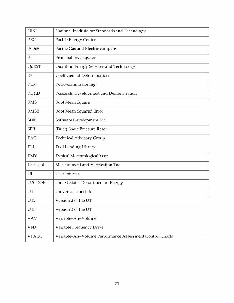
71

NIST National Institute for Standards and Technology

PEC Pacific Energy Center

PG&E Pacific Gas and Electric company

PI Principal Investigator

QuEST Quantum Energy Services and Technology

R2 Coefficient of Determination

RCx Retro‐commissioning

RD&D Research, Development and Demonstration

RMS Root Mean Square

RMSE Root Mean Squared Error

SDK Software Development Kit

SPR (Duct) Static Pressure Reset

TAG Technical Advisory Group

TLL Tool Lending Library

TMY Typical Meteorological Year

The Tool Measurement and Verification Tool

UI User Interface

U.S. DOE United States Department of Energy

UT Universal Translator

UT2 Version 2 of the UT

UT3 Version 3 of the UT

VAV Variable–Air–Volume

VFD Variable Frequency Drive

VPACC Variable–Air–Volume Performance Assessment Control Charts

72

REFERENCES

AMCA. 1990a. “Fans and Systems”. Publication 201‐90. Arlington Heights, IL: Air Movement

and Control Association International.

AMCA. 1990b. “Field Performance Measurement of Fan Systems”. Publication 203‐90.

Arlington Heights, IL: Air Movement and Control Association International.

AMCA. 2007. “ANSI/AMCA 210 (ANSI/ASHRAE 51) Laboratory Methods of Testing Fans for

Certified Aerodynamic Performance Rating”. Arlington Heights, IL: Air Movement and

Control Association International.

ASHRAE. 1999. “ANSI/ASHRAE Standard 120 Method of Testing to Determine Flow Resistance

of HVAC Ducts and Fittings”. Atlanta, GA: American Society of Heating, Refrigerating

and Air‐Conditioning Engineers, Inc.

ASHRAE. 2002. “ANSI/ASHRAE Guideline 14 Measurement of Energy and Demand Savings”.

Atlanta, GA: American Society of Heating, Refrigerating and Air‐Conditioning

Engineers, Inc.

ASHRAE. 2005. “Handbook of Fundamentals: Chapter 35, Duct Design”. Atlanta, GA:

American Society of Heating, Refrigerating and Air‐Conditioning Engineers, Inc. pp.

35.14‐35.16.

ASHRAE. 2007. “ANSI/ASHRAE Standard 90.1 Energy Standard for Buildings Except Low‐Rise

Residential Buildings”. Atlanta, GA: American Society of Heating, Refrigerating and

Air‐Conditioning Engineers, Inc.

ASHRAE. 2008a. “ANSI/ASHRAE Standard 126 Method of Testing HVAC Air Ducts and

Fittings”. Atlanta, GA: American Society of Heating, Refrigerating and Air‐Conditioning

Engineers, Inc.

ASHRAE. 2008b. “ANSI/ASHRAE Standard 111 Measurement, Testing, Adjusting, and

Balancing of Building HVAC Systems”. Atlanta, GA: American Society of Heating,

Refrigerating and Air‐Conditioning Engineers, Inc.

ASHRAE. 2012. “2012 Handbook: HVAC Systems and Equipment, Fans Chapter”. Atlanta, GA:

American Society of Heating, Refrigerating and Air‐Conditioning Engineers, Inc.

Behls, H. and C.P. Wray. “2012 ASHRAE Handbook: HVAC Systems and Equipment, Duct

Construction Chapter ‐ HVAC System Leakage”. Atlanta, GA: American Society of

Heating, Refrigerating and Air‐Conditioning Engineers, Inc.

Behls, H. and C.P. Wray. “2013 ASHRAE Handbook: Fundamentals, Duct Design Chapter ‐

HVAC System Leakage”. Atlanta, GA: American Society of Heating, Refrigerating and

Air‐Conditioning Engineers, Inc.

Brook, M. 2002. “California Electricity Outlook: Commercial Building Systems”. Presentation at

PIER Buildings Program HVAC Diagnostics Meeting, Oakland, CA. April 16.

73

Claridge, D., M. Liu, and W. Turner. 1999. “Whole–Building Diagnostics”. Proceedings of the

Diagnostics for Commercial Buildings: Research into Practice Workshop, June 16 & 17,

Pacific Energy Center, San Francisco, CA.

Diamond, R., C. Wray, D. Dickerhoff, N. Matson, and D. Wang. 2003. “Thermal Distribution

Systems in Commercial Buildings”. Lawrence Berkeley National Laboratory Report,

LBNL‐51860. http://epb.lbl.gov/publications/lbnl‐51860.pdf

Duhamel, P., and M. Vetterli. 1990. “Fast Fourier Transforms: A Tutorial Review and A State of

The Art”. Signal Processing Vol. 19, pp. 259–299.

Efficiency Valuation Organization (EVO). 2012. “International Performance Measurement and

Verification Protocol (IPMVP)”. www.evo‐world.org.

Energy Commission. 2004. “Nonresidential Alternative Calculation Method (ACM) Approval

Manual for the 2005 Building Energy Efficiency Standards for Residential and

Nonresidential Buildings”. California Energy Commission, P400‐03‐004F, October.

Franconi, E.M. 1999. “Thermodynamic Analysis for Improved HVAC Distribution System

Performance”. Ph.D. Dissertation, Department of Civil, Environmental, and

Architectural Engineering, University of Colorado, Boulder.

Geelen, B.D. 1993. “An Accurate Solution FORTRAN Algorithm for the erf and Related Error

Functions”. Advances in Engineering Software. Vol. 18, pp. 67‐71.

Grahovac, M. 2010. “Simplified Parametric Characterization of Aggregated Flow Resistances in

an Air‐Handling System Network”. Technischen Universität München, Munich,

Germany. Lawrence Berkeley National Laboratory Internship Report.

Haberl, J.S, D.E Claridge, J.K. Kissock, and T.A. Reddy. 1993. “Emodel: A New Tool for

Analyzing Building Energy Use Data”. Energy Systems Labs Report ESL‐IE‐93‐03‐33,

Texas A&M University.

Huang, J., H. Akbari, L. Rainer, and R. Ritschard. 1991. “481 Prototypical Commercial Buildings

for 20 Urban Market Areas”. Lawrence Berkeley National Laboratory Report LBL‐29798.

Hydeman, M., S. Taylor, J. Stein, E. Kolderup, and T. Hong. 2003. “Advanced Variable Air

Volume System Design Guide”. Energy Commission Report P500‐03‐082‐A‐11. October.

Ivanovich, M. 2012. “Fan Efficiency Regulations: Where Are They Going?”. Arlington Heights,

IL: AMCA International.

Kissock, J.K., Energy Explorer, software and user manual, available at:

http://academic.udayton.edu/kissock/http/RESEARCH/EnergySoftware.htm.

Kissock, J.K., J.S. Haberl, and D.E Claridge. 2002. “Development of a Toolkit for Calculating

Linear, Change‐point Linear and Multiple‐Linear Inverse Building Energy Analysis

Models”. ASHRAE Research Project 1050, Final Report, November. Atlanta, GA:

American Society of Heating, Refrigerating and Air‐Conditioning Engineers, Inc.

74

Kreider, J.F. and J.S. Haberl. 1994. “Predicting Hourly Building Energy Usage: The Results of

the 1993 Great Energy Predictor Shootout Identify the Most Accurate Method for

Making Hourly Energy Use Predictions”. ASHRAE Journal, Vol. 35, No. 3, pp. 72– 81.

Krukowski, A. and C. Wray. 2013. “Standardizing Data for VFD Efficiency”. ASHRAE Journal,

Vol. 55, No. 6. June.

Leach, M., E. Hale, A. Hirsch, and P. Torcellini. 2009. “Grocery Store 50 % Energy Savings

Technical Support Document”. National Renewable Energy Laboratory. NREL/TP‐550‐

46101.

Leach, M., C. Lobato, A. Hirsch, S. Pless, and P. Torcellini. 2010. “Technical Support Document:

Strategies for 50% Energy Savings in Large Office Buildings”. National Renewable

Energy Laboratory Report, NREL/TP‐550‐49213.

Miller, J. 2010. “Analysis of Dimensionless Models for Fan Efficiency and Speed”. University of

Rochester, NY. U.S. Department of Energy, Science Undergraduate Laboratory

Internship Report. CSEE: Center for Science and Engineering Education, Lawrence

Berkeley National Laboratory.

Modera, M.P. 2007. “Investigation of Leak Sealing for Supply and Exhaust Ductwork”.

Proceedings of the 3rd Industry Workshop on “Energy Efficient Technologies for

Buildings – New and Retrofits”. Co‐sponsored by US Department of Defense, US

Department of Energy, ASHRAE, and IEA ECBCS Annex 46. Dallas, TX. January 25‐26.

Modera, M.P., C.P. Wray, and D.J. Dickerhoff. 2013. “Low Pressure Air‐Handling System

Leakage in Large Commercial Buildings: Diagnosis, Prevalence, and Energy Impacts”.

Draft, to be submitted to ASHRAE HVAC&R Research Journal.

More, J.J. 1977. “The Levenberg‐Marquardt Algorithm: Implementation and Theory”.

Conference on Numerical Analysis, University of Dundee, Scotland. June 28‐July 1.

Argonne National Laboratory.

More, J.J., B.S. Garbow, and K.E. Hillstrom. 1980. “User Guide for MINPACK‐1”. Applied

Mathematics Division, Argonne National Laboratory. August. ANL‐80‐74.

OpenEIS. 2013. http://eis.lbl.gov

PECI. 2004. “National Strategy for Building Commissioning”. Portland Energy Conservation,

Inc. Report to U.S. Department of Energy.

Piette, M., S. Kinney, and P. Haves. 2001. “Analysis of an Information Monitoring and

Diagnostic System to Improve Building Operations”. Energy and Buildings, Vol. 33, pp.

783‐791.

Rufo, M. and F. Coito. 2002. “California Statewide Commercial Sector Energy Efficiency

Potential Study – Volume 1”. Final Report of XENERGY Inc., Regional Economic

Research Inc., Quantum Consulting Inc., and Energy Solutions Inc. to Pacific Gas &

75

Electric Company, San Francisco, CA. July.

http://www.calmac.org/publications/CA_EEPotV1.pdf.

Schein, J. 2006. “Results from Field Testing of Embedded Air Handling Unit and Variable Air

Volume Box Fault Detection Tools”. National Institute of Standards and Technology

Report, NISTIR 7365. http://www.nist.gov/customcf/get_pdf.cfm?pub_id=861015

Sherman, M.H. and C.P. Wray. 2010. “Parametric System Curves: Correlations between Fan

Pressure Rise and Flow for Large Commercial Buildings”. Lawrence Berkeley National

Laboratory Report. LBNL‐3542E.

Subbarao, K., L. Yafeng, and T.A. Reddy. 2011. “The Nearest Neighbor Method to Improve

Uncertainty Estimates in Statistical Building Energy Models”. ASHRAE Transactions,

pp. 459‐471.

Summers, H. and C. Hilger. 2012. “Fault Detection and Diagnostic Software”. Emerging

Technologies Program Report ET11PGE3131, Pacific Gas and Electric Company, San

Francisco, CA.

TIAX. 2002. “Energy Consumption Characteristics of Commercial Building HVAC Systems,

Volume III, Energy Savings Potential”. Final Report to U.S. Department of Energy,

Office of Building Technologies.

Ulickey, J., Fackler, T., Koeppel, and E., Soper, J. 2010. “Characterization of Fault Detection and

Diagnostic (FDD) and Advanced Energy Information System (EIS) Tools”, Task 4.3

Report: Project “Performance Tracking in Large Commercial Buildings: Tools and

Strategies” to California Commissioning Collaborative, California Energy Commission,

September.

U.S. DOE. 2013. “EnergyPlus Engineering Document: The Reference to EnergyPlus

Calculations”. Board of Trustees of the University of Illinois and Regents of the

University of California through the Ernest Orlando Lawrence Berkeley National

Laboratory, U.S. Department of Energy. May 16.

Webster, T. and A. Barth. 2003. “High Performance Commercial Building Systems:

Development of Fan Diagnostic Methods and Protocols for Short Term Monitoring”.

Center for Environmental Design Research, University of California, Berkeley and

Nexant Energy Management Group Report to California Energy Commission Public

Interest Energy Research Program. HPCBS# E5P2.2T4d. February.

Webster, T., E. Ring, Q. Zhang, C. Huizenga, F. Bauman, and E. Arens. 1999. “Commercial

Thermal Distribution Systems: Reducing Fan Energy in Built‐Up Fan Systems”. Final

Report of Lawrence Berkeley National Laboratory and Center for Environmental Design

Research, University of California Berkeley to California Institute for Energy Efficiency

and the California Energy Commission. LBNL‐44320. December.

Westphalen, D. and K. Roth. 2003. “System and Component Diagnostics”. ASHRAE Journal,

Vol. 45, No. 4.

76

Wray, C.P., R.C. Diamond, and M.H. Sherman. 2005. “Rationale for Measuring Duct Leakage

Flows in Large Commercial Buildings”. Proceedings – 26th AIVC Conference, Brussels,

Belgium, September. LBNL‐58252. http://epb.lbl.gov/publications/lbnl‐58252.pdf

Wray, C.P. 2012a. “Fan Airflow and Pressure Rise: Can We Measure In‐Situ Performance?”.

Seminar, ASHRAE Winter Meeting, Chicago, IL. January.

Wray, C.P. 2012b. “Energy Impacts of Air‐Handling System Leakage in Large Commercial

Buildings: Measurements and Simulation”. Seminar, ASHRAE Winter Meeting, Chicago,

IL. January.

Wright, J. 2011. “Chapter 11: HVAC Systems Performance Prediction”. In Building Performance

Simulation for Design and Operation, J.L.M. Hensen and R. Lamberts, ed. New York, NY:

Spoon Press.

Date post:	19-Mar-2018
Category:	Documents
Upload:	dangdung
View:	213 times
Download:	0 times

Development of Diagnostic, and Measurement and ... · PDF fileDevelopment of Diagnostic, and...

Documents