TRB 2007 Annual Meeting – Initial Submittal for Review DEVELOPMENT OF FATIGUE CRACKING PERFORMANCE PREDICTION MODELS FOR FLEXIBLE PAVEMENTS USING LTPP DATABASE Submitted for Presentation and Publication at the 86 th Annual Meeting of the Transportation Research Board Washington, D.C. January 21-25, 2007 Hsiang-Wei Ker, Ph.D. Associate Professor Department of International Trade, Chihlee Institute of Technology #313, Sec. 1, Wen-Hwa Rd., Pan-Chiao, Taipei, Taiwan 220 TEL: (886-2) 2257-6167 Ext 553 E-mail: [email protected]Ying-Haur Lee, Ph.D. (Corresponding Author) Professor Department of Civil Engineering, Tamkang University E732, #151 Ying-Chuan Rd., Tamsui, Taipei, Taiwan 251 TEL/FAX: (886-2) 2623-2408 E-mail: [email protected]Pei-Hwa Wu, Ressearch Assistant Department of Civil Engineering, Tamkang University E801, #151 Ying-Chuan Rd., Tamsui, Taipei, Taiwan 251 TEL/FAX: (886-2) 2621-5656 Ext 2671 Text: 4,165 Words Figures: 10*250=2,500 Words Tables: 2*250= 500 Words Total: 7,165 Words Originally Submitted on July 31, 2006 (First Revision Made on October 28, 2006)
Transcript
TRB 2007 Annual Meeting – Initial Submittal for Review
DEVELOPMENT OF FATIGUE CRACKING PERFORMANCE PREDICTION MODELS FOR FLEXIBLE PAVEMENTS
USING LTPP DATABASE
Submitted for Presentation and Publication at the 86th Annual Meeting of the
Transportation Research Board
Washington, D.C. January 21-25, 2007
Hsiang-Wei Ker, Ph.D. Associate Professor Department of International Trade, Chihlee Institute of Technology #313, Sec. 1, Wen-Hwa Rd., Pan-Chiao, Taipei, Taiwan 220 TEL: (886-2) 2257-6167 Ext 553 E-mail: [email protected] Ying-Haur Lee, Ph.D. (Corresponding Author) Professor Department of Civil Engineering, Tamkang University E732, #151 Ying-Chuan Rd., Tamsui, Taipei, Taiwan 251 TEL/FAX: (886-2) 2623-2408 E-mail: [email protected]
Pei-Hwa Wu, Ressearch Assistant Department of Civil Engineering, Tamkang University E801, #151 Ying-Chuan Rd., Tamsui, Taipei, Taiwan 251 TEL/FAX: (886-2) 2621-5656 Ext 2671
Text: 4,165 Words Figures: 10*250=2,500 Words Tables: 2*250= 500 Words Total: 7,165 Words Originally Submitted on July 31, 2006 (First Revision Made on October 28, 2006)
Ker, Lee, and Wu
TRB 2007 Annual Meeting – Initial Submittal for Review
2
Development of Fatigue Cracking Performance Prediction Models for Flexible Pavements Using LTPP Database
H. W. Ker, Y. H. Lee, and P. H. Wu
Abstract: The main objective of this study is to develop improved fatigue cracking models for flexible pavements using the Long-Term Pavement Performance (LTPP) database. The retrieval, preparation, and cleaning of the database were carefully handled in a more systematic and automatic approach. The prediction accuracy of the existing prediction models implemented in the recommended Mechanistic-Empirical Pavement Design Guide (NCHRP Project 1-37A) was found to be inadequate. Exploratory data analysis indicated that the normality assumption with random errors and constant variance using conventional regression techniques might not be appropriate for this study. Therefore, several modern regression techniques including generalized linear model (GLM) and generalized additive model (GAM) along with the assumption of Poisson distribution and quasi-likelihood estimation method were adopted for the modeling process. The resulting mechanistic-empirical model included several variables such as yearly KESALs, pavement age, annual precipitation, annual temperature, critical tensile strain under the AC surface layer, and freeze-thaw cycle for the prediction of fatigue cracking. The goodness of the model fit was further examined through the significant testing and various sensitivity analyses of pertinent explanatory parameters. The tentatively proposed predictive models appeared to reasonably agree with the pavement performance data although their further enhancements are possible and recommended.
INTRODUCTION
Performance predictive models have been used in various pavement design, evaluation, rehabilitation, and network management activities. Since fatigue cracking is one of the major flexible pavement distress types primarily caused by the accumulated traffic loads. Extensive research has been conducted to predict the occurrence of this distress type using various empirical and mechanistic-empirical approaches. Conventional predictive models usually correlate fatigue damage to the critical tensile strain and the stiffness of the AC surface layer (1). As pavement design evolves from traditional empirically based methods toward mechanistic-empirical, the equivalent single axle load (ESAL) concept used for traffic loads estimation is no longer adopted in the recommended Mechanistic-Empirical Pavement Design Guide (MEPDG) (NCHRP Project 1-37A) (2). The success of the new design guide considerably depends upon the accuracy of pavement performance predictions. Thus, this study will first investigate its goodness of fit and strive to develop improved fatigue cracking prediction models for flexible pavements using the Long-Term Pavement Performance (LTPP) database (http://www.datapave.com or LTPP DataPave Online) (3-5).
BRIEF REVIEW OF EXISTING MECHANISTIC-EMPIRICAL PREDICTION MODELS
Since fatigue cracking is primarily caused by accumulated traffic loads, various predictive models as shown in Table 1 based on the following expressions have been proposed to estimate the maximum allowable number of repetitions (Nf) using the critical tensile strain (εt) and the dynamic modulus (E*) of AC surface layer (6-9):
32 *
1 )(kk
tf EkN−−= ε (1)
TABLE 1 Models for Predicting Allowable Load Repetitions (7) Organization Author (Year) k1 k2 k3 Asphalt Institute AI (1981) 0.0796 3.291 0.854Shell Oil Shook (1982) 0.0685 5.671 2.363Belgian Road Research Center Verstraeten (1984) 4.92×10⁻¹⁴ 4.76 0UC-Berkeley Craus (1984) 0.0636 3.291 0.854Transport and Road Research Laboratory Powell (1984) 1.66×10⁻¹⁰ 4.32 0Illinois Thompson (1987) 5×10⁻⁶ 3.0 0U.S. Army Department of Defense (1988) 478.63 5.0 2.66Indian Das, Pandey (1999) 0.1001 3.565 1.474Mn/ROAD Timm (2003) 2.83 3.21 0
Ker, Lee, and Wu
TRB 2007 Annual Meeting – Initial Submittal for Review
3
In which, k1, k2, and k3 are regression coefficients. The pavement is considered to be failed when there exists 20 percent of fatigue cracking in the entire lane area (or equivalent to 45 percent in the wheel path area) (10). Cumulative fatigue damage (Df) is then calculated by adding the damage caused by each individual load application based on Miner’s hypothesis:
∑=
=k
i fi
if N
nD1
(2)
Where, k is the number of axle load type, ni is the number of axle applications, and Nfi is the corresponding maximum allowable number of repetitions.
In the recommended MEPDG, the revised MS-1 fatigue cracking model which was originally developed by Asphalt Institute for bottom up alligator cracking is shown as follows (2, Appendix II-1):
⎟⎟⎠
⎞⎜⎜⎝
⎛−
+=
⎟⎠⎞
⎜⎝⎛
⎟⎟⎠
⎞⎜⎜⎝
⎛=
69.0*84.4
*854.0*291.3
1
10
11***00432.032
ba
b
ff
VVV
tff
C
ECN
ββ
εβ
(3)
Where, βf1, βf2, βf3 are calibration factors; βf1=β′f1*k′1; β′f1 is a numerical value; k′1 is a function of the AC layer thickness; C is laboratory to field adjustment factor; εt is the critical tensile strain and E is the stiffness of the AC surface layer; Va stands for air voids (%); and Vb is the effective binder content (%). The alligator cracking model calibration process included the following steps: estimation of coefficients βf2 and βf3 for the MS-1 number of load repetitions; finding the fatigue cracking damage transfer function by correlating fatigue cracking with the damage using only sections with AC layer thickness greater than 4 inches; and then shifting the thin sections using the k′1parameter. The results showed that choosing βf2 equal to 1.2 and βf3 equal to 1.5 provided a more realistic prediction. The final transfer function to calculate fatigue cracking from cumulative fatigue damage (Df) is based on the assumption that the alligator cracking of the total lane area would be 50% at a fatigue damage of 100%. The calibrated model for the bottom up fatigue cracking (F.C., %) is as follows:
⎟⎠⎞
⎜⎝⎛
⎟⎟⎠
⎞⎜⎜⎝
⎛
+= ′+′ 60
1*1
6000.. ))100*log(***( 2211 fDCCCCeCF (4)
In which, C1=1.0; C2=1.0; C′1= -2* C′2; C′2= -2.40874-39.748*(1+hac)-2.856; and hac is the total thickness of the asphalt concrete layer (in.). The fatigue damage is calculated in a similar way using equation (2) based on more complex Axle Load Spectra (ALS) concept.
DATABASE PREPARATION
Initially, the DataPave 3.0 program was used to prepare a database for this study. However, in order to obtain additional variables and the latest updates of the data, the Long-Term Pavement Performance database retrieved from http://www.datapave.com (or LTPP DataPave Online, Release 18.0) (4) became the main source for this study. Starting from 1987, the LTPP program has been monitoring more than 2,400 asphalt and Portland cement concrete pavement test sections across the North America. Very detailed information about original construction, pavement inventory data, materials and testing, historical traffic counts, performance data, maintenance and rehabilitation records, and climatic information have been collected. There are 8 general pavement studies (GPS) and 9 specific pavement studies (SPS) in the LTPP program. Of which, only asphalt concrete (AC) pavements on granular base (GPS1) and on bound base (GPS2) was used for this study.
This database is currently implemented in an information management system (IMS) which is a relational database structure using the Microsoft Access program. Automatic summary reports of the pavement information may be generated from different IMS modules, tables, and data elements. The thickness of pavement layers was obtained from the IMS Testing module rather than the IMS Inventory module to be consistent with the results of Section Presentation module in the DataPave 3.0 program. Several other material properties such as air voids, effective binder content, etc were queried from the Inventory module. Detailed traffic counts and equivalent single axle load (ESAL) were obtained from the Traffic module. The cumulated ESAL during the
Ker, Lee, and Wu
TRB 2007 Annual Meeting – Initial Submittal for Review
4
performance analysis period was calculated by multiplying pavement age with mean yearly ESAL (or kesal) which could be easily estimated from the database. Environmental data were retrieved from the IMS Climate module and the associated Virtual Weather Station (VWS) link. The alligator cracking data (including low, medium, and high severities) used in this study was obtained from MON_DIS_AC_REV table in the IMS Monitoring module. Maintenance and rehabilitation activities could effectively reduce the distress quantities. Thus, the records in both Maintenance and Rehabilitation modules were used to assure that this study only chose the performance data of those sections without or before major improvements.
For the purpose of this study, a Microsoft Excel summary table containing the pavement inventory, material and testing, traffic, climatic, and distress data was created using the relational database features of the Access program. The Excel table was then stored as S-Plus datasets for subsequent analysis. The summary, table, cor, plot, pairs, and coplot functions were heavily utilized to summarize the information of interest and to provide more reliable data for this study. To estimate the critical tensile strain (εt) of the AC surface layer, a systematic approach was utilized and implemented in a Visual Basic software package to automatically read in the pavement inventory data from the summary table, generate the BISAR input files, conduct the batch runs, as well as summarize the results (3). In which, the static (or laboratory tested) elastic modulus data recorded in the IMS Testing module and a single wheel load of 40 kN (9,000 lbs) with a tire pressure of 0.482 MPa (70 psi) were used for the analysis.
Furthermore, the aforementioned mechanistic-empirical models also require the dynamic Young’s modulus of AC surface layer. LTPP program utilized the MODCOMP4 program to (11) backcalculate the dynamic modulus of each pavement layer which could be retrieved from the IMS Monitoring module. Thus, it would be interesting to compare the laboratory tested layer moduli versus the backcalculated dynamic Young’s moduli so as to have a better understanding of their associated variability. As shown in Figure 1, the variability of the relationship between the dynamic and the static (or laboratory tested) moduli could not be ignored. The average ratios of which are approximately 2.6, 2.7, 7.3, and 3.4 by eliminating some apparent outliers for AC surface, base, subbase, and subgrade layers, respectively.
(a) (b)
2000 4000 6000 8000 10000
5000
1000
015
000
2000
025
000
3000
0
100 150 200 250
050
010
0015
00
(c) (d)
50 100 150 200 250
020
0040
0060
0080
00
50 100 150
050
010
0015
00
FIGURE 1 Comparison of layer moduli of (a) AC surface layer; (b) base layer; (c) subbase layer; and (d) subgrade obtained from laboratory testing (x axis, MPa) and backcalculation program (y axis, MPa).
A data cleaning process must be conducted before any preliminary analysis or regression analysis can be performed. With the help of graphical representation, fatigue cracking data were plotted against surveyed
Ker, Lee, and Wu
TRB 2007 Annual Meeting – Initial Submittal for Review
5
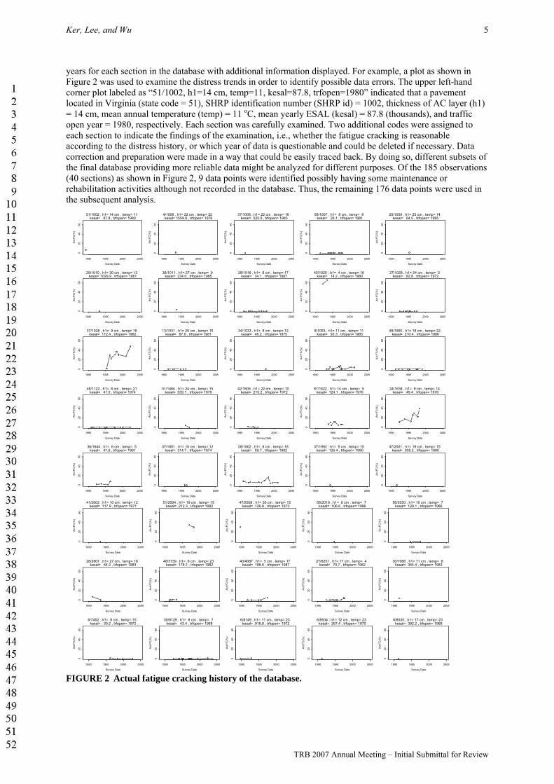
years for each section in the database with additional information displayed. For example, a plot as shown in Figure 2 was used to examine the distress trends in order to identify possible data errors. The upper left-hand corner plot labeled as “51/1002, h1=14 cm, temp=11, kesal=87.8, trfopen=1980” indicated that a pavement located in Virginia (state code = 51), SHRP identification number (SHRP id) = 1002, thickness of AC layer (h1) = 14 cm, mean annual temperature (temp) = 11 oC, mean yearly ESAL (kesal) = 87.8 (thousands), and traffic open year = 1980, respectively. Each section was carefully examined. Two additional codes were assigned to each section to indicate the findings of the examination, i.e., whether the fatigue cracking is reasonable according to the distress history, or which year of data is questionable and could be deleted if necessary. Data correction and preparation were made in a way that could be easily traced back. By doing so, different subsets of the final database providing more reliable data might be analyzed for different purposes. Of the 185 observations (40 sections) as shown in Figure 2, 9 data points were identified possibly having some maintenance or rehabilitation activities although not recorded in the database. Thus, the remaining 176 data points were used in the subsequent analysis.
FIGURE 2 Actual fatigue cracking history of the database.
Ker, Lee, and Wu
TRB 2007 Annual Meeting – Initial Submittal for Review
6
PRELIMINARY ANALYSIS OF THE FATIGUE CRACKING DATABASE
Univariate Data Analysis Univariate data analysis consists of statistical methods for describing the distribution and spread of each individual variable. Some basic descriptive statistics regarding the data range, its variation, and the number of missing values for each individual variable are given in Table 2. Univariate data analysis procedure is often used to investigate the possibility of data errors and potential distribution problem for each variable considered in a regression analysis. A few extreme (or unusual) data points may be identified or deleted from the analysis. In which, age stands for pavement age (years); cesal is the cumulative ESALs (millions); kesal is the yearly ESALs (thousands); h1 and h2 are the thickness of the AC surface layer and base layer (cm), respectively; e1 is the stiffness of the AC layer (MPa); epsilon.t (εt) is critical tensile strain; ft is yearly freeze-thaw cycle; temp is mean annual temperature (oC); precip is mean annual precipitation (mm); act.fc is actual fatigue cracking (%).
A graph is always far more perceptible than thousands of numbers. A single plot which well describes the spread of the data may be created by combining these univariate statistics with a histogram. A simplified distribution plot which graphically displays the variability of data including median, lower and upper quantiles, 95 percent confidence intervals, and extreme points (if any) may be made in a boxplot. A boxplot displays not only the location and spread of the data but also skewness as well. A histogram only displays a rough and crude shape of the distribution of data. To have a smoother look, a continuous curve of the nonparametric estimate of the probability density may also be obtained. A normal probability plot or a quantile-quantile plot can be used to have a quick visual check on the assumption of normal distribution. If the distribution is close to normal, the plot will show approximately a straight-line relationship (12, 13). The distribution of fatigue cracking (act.fc) is shown in Figure 3. The solid horizontal white line in the box plot indicates the median of the data whereas the
Ker, Lee, and Wu
TRB 2007 Annual Meeting – Initial Submittal for Review
7
upper and lower ends of the box show the upper and lower quantiles, respectively. These plots reveal a relatively skewed distribution for actual fatigue cracking.
0 20 40 60
050
100
150
act.fc
Cou
nt
010
2030
4050
60
act.f
c
act.fc
Den
sity
0 20 40 60
0.0
0.05
0.10
0.15
Quantiles of Standard Normal
act.f
c
-2 -1 0 1 2
010
2030
4050
60
FIGURE 3 Exploratory data analysis: fatigue cracking of flexible pavements.
Bivariate and Multivariate Analysis A correlation matrix of these variables is also given in Table 2. In addition, trimmed correlation matrices show the variable correlations after a certain portion of influential data points or possible outliers are eliminated (say 3 percent in this example) such that more reliable indices of the correlations are obtained. Note the difference between the resulting traditional correlation matrix and trimmed correlation matrix. A scatter plot matrix can graphically represent their relationships and scatters. Applying a data smoothing technique (lowess) on the same scatter plot matrix, the pairwise relationships as shown in Figure 4 become clearer and possible data errors may also be easily identified (12, 13).
INVESTIGATION OF THE EXISTING PREDICTIVE MODELS
To investigate the goodness of prediction, cumulative fatigue damage (Df) was calculated and plotted against the actual fatigue cracking using equations (1) and (2) and the coefficients given in Table 1 for AI, Shell Oil, U.S. Army, and Mn/Road models. Except for the Mn/Road model, the results of this analysis are quite similar as depicted in Figure 5.
Together with the aforementioned AI model, the following relationship developed by Ali and Tayabji (9, 14) was adopted to illustrate the goodness of fatigue cracking predictions using LTPP GPS-1 data (AC pavements on granular base) as shown in Figure 6.
( )fDeckingFatigueCra *85.0027.0
021.0% −+= (5)
Ker, Lee, and Wu
TRB 2007 Annual Meeting – Initial Submittal for Review
FIGURE 4 Using scatter plot smoother (lowess) on the scatter plot matrix. (a) (b)
log Σni/Nfi
Act
.Fat
igue
Cra
ckin
g[%
]
-6 -4 -2 0
010
2030
4050
60
log Σni/Nfi
Act
.Fat
igue
Cra
ckin
g[%
]
-8 -6 -4 -2 0 2
010
2030
4050
60
(c) (d)
log Σni/Nfi
Act
.Fat
igue
Cra
ckin
g[%
]
-6 -4 -2 0 2
010
2030
4050
60
log Σni/Nfi
Act
.Fat
igue
Cra
ckin
g[%
]
-12 -11 -10 -9 -8 -7
010
2030
4050
60
FIGURE 5 Comparison of prediction results using (a) AI model; (b) Shell Oil model; (c) U.S. Army model; and (d) Mn/Road model.
Ker, Lee, and Wu
TRB 2007 Annual Meeting – Initial Submittal for Review
9
FIGURE 6 Prediction results using AI model together with equation (5) for LTPP GPS-1 data.
The prediction accuracy of the proposed models implemented in the recommended MEPDG (NCHRP Project 1-37A) was further investigated. To avoid undesirable misunderstanding of the new guide’s prediction algorithm due to the complexity involved, it was decided to directly use the MEPDG software for the prediction of alligator cracking. The beta version of the software could be downloaded from http://www.trb.org/mepdg/ software.htm. The goodness of fatigue cracking prediction using AI model and equation (5) as well as the recommended MEPDG models is shown in Figure 7. Unfortunately, the prediction accuracy of the existing prediction models was found to be inadequate.
DEVELOPMENT OF IMPROVED FATIGUE CRACKING MODELS
The occurrence of fatigue cracking in field depends on various factors namely traffic, environment, structure, construction, maintenance and rehabilitation. Wang et al. (15) developed a relationship to predict the median failure time due to fatigue cracking using the following explanatory parameters: traffic (different ESAL levels), thickness of AC layer, thickness of base layer, mean annual precipitation, and freeze-thaw cycles per year. Thus, it is prudent to develop improved fatigue cracking prediction models using not only the critical strain and the stiffness of AC layer but the aforementioned parameters as well. (a) (b)
Act. Fatigue Cracking (%)
Pre
. Fat
igue
Cra
ckin
g (%
)
0 10 20 30 40
020
4060
8010
0
Act. Fatigue Cracking (%)
Pre
. Fat
igue
Cra
ckin
g (%
)
0 10 20 30 40
020
4060
8010
0
FIGURE 7 Comparison of goodness of fatigue cracking prediction using (a) AI model; and (b) MEPDG models.
To develop a more reliable predictive model for practical engineering problems, Lee and Darter (16, 17) proposed a predictive modeling approach to incorporate robust (least median squared) regression, alternating conditional expectations, and additivity and variance stabilization algorithms into the modeling process. The robust regression is proposed due to its favorable feature of analyzing highly contaminated data by detecting outliers from both dependent variable and independent variables. Through the iterative use of the combination of these outlier detection and nonparametric transformation techniques, it is believed that some potential outliers and proper functional forms may be identified. Subsequently, traditional regression techniques can be more easily utilized to develop the final predictive model. Nevertheless, many preliminary trials using these regression techniques have shown extreme difficulty to achieve a satisfactory predictive model for this set of data.
Exploratory data analysis of the response variable as shown in Figure 3 indicated that the normality assumption with random errors and constant variance using conventional regression techniques might not be appropriate for prediction modeling. The Shapiro-Wilk W-statistic for testing for departures from normality was
0 10 20 30 40 50 60 70Actual Fatigue Cracking (%)
0
8
16
Pre
dict
ed F
atig
ue C
rack
ing
(%)
Ker, Lee, and Wu
TRB 2007 Annual Meeting – Initial Submittal for Review
10
also used to test the distribution of fatigue cracking (12, 13). Apparently, the logarithm of fatigue cracking has better data scatter, though the W-statistic still indicated that the distribution of fatigue cracking is not lognormal distributed. Furthermore, since various distribution functions have been assumed for fatigue cracking analysis in the literature (2, Appendix II-1; 15), the Kolmogorov-Smirnov goodness-of-fit test was also used to test whether the fatigue cracking could be characterize by normal, exponential, gamma, lognormal, or Poisson distribution (13). Unfortunately, no apparent conclusion in distribution function selection could be reached for this dataset.
Preliminary Models Using Poisson Regression Techniques
“When events of a certain type occur over time, space, or some other index of size, it is often relevant to model the rate at which events occur (18).” Due to the data collecting nature of fatigue cracking, it could be treated as rate data, i.e., percent of the entire lane area. Agresti (18) also suggested that using Poisson regression for rate data is an appropriate decision. Therefore, generalized linear model (GLM) (19) along with the assumption of Poisson distribution was adopted in this analysis. In which, a Poisson loglinear model is a GLM that assumes a Poisson distribution for the response variable and uses the log link. After going through several trails in eliminating insignificant and/or inappropriate parameters, the following model was obtained:
In which, dispersion parameter for Poisson family taken to be 1; null deviance = 2536.613 on 175 degrees of freedom; residual deviance = 1403.364 on 169 degrees of freedom; age stands for pavement age (years); kesal is the yearly ESALs (thousands); precip stands for mean annual precipitation (mm); temp stands for mean annual temperature (oC); epsilon.t (εt) is the critical tensile strain; ft stands for yearly freeze-thaw cycle; FC is fatigue cracking in percent of entire lane area (%).
Figure 8 shows two diagnosing plots of the above model. A plot of residuals versus the fitted values can be used to check the adequacy of the model. If any curvature is observed, then the model might be improved by adding additional, nonlinear terms to the model. A plot of the response versus fitted values is always provided to illustrate the goodness of the fit. Since the main objective is to predict the rate of fatigue cracking, it is desirable to rearrange the above equation into the following expression and obtain new regression summary statistics:
Note that R2 is the coefficient of determination, SEE is the standard error of estimate and n is the number of observations.
(a) (b)
Fitted : age + kesal + precip + temp + epsilon.t + ft
Dev
ianc
e R
esid
uals
0 10 20 30
-50
510
Fitted : age + kesal + precip + temp + epsilon.t + ft
act.f
c
0 10 20 30 40 50 60
010
2030
4050
60
FIGURE 8 Diagnosis plots of the preliminary Poisson loglinear model: (a) residuals against fitted values; and (b) response against fitted values.
Ker, Lee, and Wu
TRB 2007 Annual Meeting – Initial Submittal for Review
11
To improve the model fits, it is possible to develop separate models for different climatic zones to account for other factors not considered in the above model implicitly. Due to the unbalanced data structure, of which 38, 85, 48, and 5 data points were obtained from Wet-Freeze, Wet-NonFreeze, Dry-Freeze, and Dry-NonFreeze zones, respectively, the following models were develop by regrouping the data into either Wet or Dry, or Freeze or NonFreeze zones:
Also note that new variables such as the viscosity of the AC layer (visco) and temperature range (trange, oC) were included to improve the model fits after eliminating some insignificant and inappropriate parameters. In which, trange is defined as the difference of maximum and minimum mean annual temperature.
Proposed Model Using Additional Modern Regression Techniques
Since the primary assumption of the above preliminary GLM models is that a linear function of the parameters was used in the model. Generalized additive model (GAM) extends GLM by fitting nonparametric functions using data smoothing techniques to estimate the relationship between the response and the predictors (13). To further enhance the model fits, generalized additive model (GAM) techniques were adopted in this analysis. Box-Cox power transformation technique was routinely utilized to estimate a proper, monotonic transformation for each variable based on the resulting preliminary GAM model. The fatigue cracking data was refitted with these transformed predictors using generalized linear model (GLM) techniques. To alleviate the assumption of Poisson distribution, the quasi-likelihood estimation method was also used to estimate regression relationships without fully knowing the error distribution of the response variable. Visual graphical techniques as well as the systematic statistical and engineering approach proposed by Lee (16, 17) were frequently adopted during the prediction modeling process.
After considerable amount of trails, the quasi family with the same link and variance functions from Poisson family appeared to be the best choice among several different distribution functions conducted in this analysis, i.e., normal/Gaussian, gamma, Poisson, and quasi (12, 13). Note that the Poisson family is useful for modeling count or rate data that typically follows a Poisson distribution. Consequently, the proposed model for predicting the fatigue cracking of AC pavements (in percent of entire lane area) is given as follows:
( )()
176n 7.605,SEE 0.4967,R :Statistics
)log(*242.3)1000*.(*489.31*869.0
*121.0log*832.0*943.008.18exp
2
2
===
+++
+++−=
fttepsilontemp
precipkesalageFC
(12)
In which, the dispersion parameter for quasi-likelihood family was taken to be 7.701441, suggesting over-dispersion; null deviance = 2536.613 on 175 degrees of freedom; and residual deviance = 1160.759 on 169 degrees of freedom. Figure 9 displays two diagnosing plots of the proposed model. No apparent curvature is
Ker, Lee, and Wu
TRB 2007 Annual Meeting – Initial Submittal for Review
12
observed in the residual plot, which is considered to have significant improvements over that reported in the Appendix II-1 of the recommended MEPDG (NCHRP Project 1-37A) (2). The plot of the response versus fitted values also showed that the proposed model has substantial improvements over the existing models (as shown in Figure 7 and in the above reference) in an attempt to uncover the underlying relationships.
(a) (b)
FIGURE 9 Diagnosis plots of the proposed model: (a) residuals against fitted values; and (b) response against fitted values.
Sensitivity Analysis of the Proposed Model
The goodness of the model fit was further examined through the significant testing and various sensitivity analyses of pertinent explanatory parameters. Some plots showing the sensitivity of the various factors in the proposed model are presented in Figure 10. These plots were prepared based on the range of the actual data while setting the remaining parameters to the corresponding mean values as shown in Table 2. The plots show the relationships among yearly ESAL (kesal), pavement age (age), the critical strain of AC layer (epsilon.t), mean annual precipitation (precip, mm), yearly freeze-thaw cycle (ft), and the predicted fatigue cracking (pre.fc, %). The general trends of these effects seem to be fairly reasonable.
DISCUSSIONS AND CONCLUSIONS
The prediction accuracy of the existing fatigue cracking models for flexible pavements using the Long-Term Pavement Performance (LTPP) database was found to be inadequate and greatly in need for improvement. A relatively skewed distribution for actual fatigue cracking was identified, which also indicated that normality assumption using conventional regression techniques might not be appropriate for this study. Thus, generalized linear model (GLM) and generalized additive model (GAM) along with the assumption of Poisson distribution and quasi-likelihood estimation method were adopted for the modeling process.
After many trails in eliminating insignificant and inappropriate parameters, the resulting proposed model included several variables such as yearly KESALs, pavement age, annual precipitation, annual temperature, critical tensile strain under the AC surface layer, and freeze-thaw cycle for the prediction of fatigue cracking. The goodness of the model fit was further examined. The residual plot and the plot of the response versus fitted values all indicated that the proposed model has substantial improvements over the existing models. Sensitivity analysis of the explanatory variables indicated their general trends seem to be fairly reasonable. The tentatively proposed predictive models appeared to reasonably agree with the pavement performance data although their further enhancements are possible and recommended.
ACKNOWLEDGMENTS
This study was sponsored by National Science Council, Taiwan, under the project titled “Development and Applications of Pavement Performance Prediction Models,” Phase I (NSC 93-2211-E-032-016) and Phase II (NSC94-2211-E032-014). Technical guidance provided by Dr. Ming-Jen Liu and Dr. Shao-Tang Yen is gratefully acknowledged.
Dev
ianc
e R
esid
uals
0 10 20 30
-50
5
act.f
c
0 10 20 30 40 50 60
010
2030
4050
60
Fitted Values Fitted Values
Ker, Lee, and Wu
TRB 2007 Annual Meeting – Initial Submittal for Review
13
200 400 600 800 1000 12001400
kesal0.05
0.1
0.15
0.2
0.25
0.3
epsilon.t (*1000)
010
2030
40pr
e.fc
510
1520
2530
age0.05
0.1
0.15
0.2
0.25
0.3
epsilon.t (*1000)
010
2030
4050
6070
pre.
fc
510
1520
2530
age200
400
600
800
1000
1200
1400
kesal
05
1015
2025
pre.
fc
200 400 600 800 1000 1200 1400
precip20
4060
80100
120140
ft
05
1015
2025
pre.
fc
FIGURE 10 Sensitivity analysis of the proposed model.
REFERENCES
1. Shell International Petroleum Company. Shell Pavement Design Manual-Asphalt Pavements and Overlays for Road Traffic, London, 1978. 2. ARA, Inc. ERES Consultants Division, Guide for Mechanistic-Empirical Design of New and Rehabilitated Pavement Structure, NCHRP Research 1-37A Report, TRB, National Research Council, Washington, D.C., 2004. 3. FHWA. Distress Identification Manual for the Long-Term Pavement Performance Program, Publication No. FHWA-RD-03-031, 2003. 4. FHWA. Long-Term Pavement Performance Information Management System: Pavement Performance Database Users Reference Guide, Publication No. FHWA-RD-03-088, 2004. 5. Wu, P. H. Development of Performance Prediction Models for Flexible Pavements, Master Thesis, Tamkang University, Taiwan, 2006. (In Chinese) 6. Asphalt Institute. Research and Development of the Asphalt Institute’s Thickness Design Manual (MS-1), 9th Ed., Research Report 82-2, 1982. 7. Lin, J. H. The Effects of Heavy Vehicle and Environmental Factors on Flexible Pavements, M.S. Thesis, National Central University, Chung-Li, Taoyuan, Taiwan, 2003. (In Chinese) 8. Huang, Y. H. Pavement Analysis and Design, 2nd Ed., Prentice Hall, New Jersey, 2004. 9. FHWA. Mechanistic Evaluation of Test Data from LTPP Flexible Pavement Test Sections, Final Report, Vol. 1, Publication No. FHWA-RD-98-020, 1998. 10. Strategic Highway Research Program. Early Analyses of LTPP General Pavement Studies Data, Volume 3-Sensitivity Analyses for Selected Pavement Distresses, 1993. 11. FHWA. Back-Calculation of Layer Parameters for LTPP Test Sections Volume Ⅱ: Layered Elastic Analysis for Flexible and Rigid Pavements, Publication No. FHWA-RD-01-113, 2002. 12. Insightful Corp. S-Plus 6.2 for Windows: User’s Manual, Language Reference, 2003. 13. Venables, W. N., and B. D. Ripley. Modern Applied Statistics with S. 4th Ed., New York: Springer-Verlag, 2002.
Ker, Lee, and Wu
TRB 2007 Annual Meeting – Initial Submittal for Review
14
14. Ali, H. A., and S. D. Tayabji. Evaluation of Mechanistic-Empirical Performance Prediction Models for Flexible Pavement. In Transportation Research Record, No. 1629, TRB, National Research Council, Washington, D.C., 1998, pp.169-180. 15. Wang, Y., K. C. Mahboub, and D. E. Hancher. Survival Analysis of Fatigue Cracking for Flexible Pavement Based on Long-Term Pavement Performance Data, Journal of Transportation Engineering, Vol. 131, No.8 , August 2005. 16. Lee Y. H. Development of Pavement Prediction Models, Ph.D. Dissertation, University of Illinois, Urbana, 1993. 17. Lee, Y. H., and M. I. Darter Development of Performance Prediction Models for Illinois Continuously Reinforced Concrete Pavements. In Transportation Research Record, No. 1505, TRB, National Research Council, Washington, D.C., 1995, pp. 75-84. 18. Agresti, A. An Introduction to Categorical Data Analysis, John Wiley & Sons, Inc., 1996. 19. Nelder, J. A., and R. W. M. Wedderburn, Generalized Linear Models, Journal of the Royal Statistical Society (Series A), Vol. 135, 1972, pp. 370-384.