Page 1
DEVELOPMENT OF ITERATIVE ANALYTICAL PROCEDURE
FOR BOILER TUBE ANALYSIS IN MATLAB
ANG WEI BING
A project report submitted in partial fulfilment of the
requirements for the award of Bachelor of Engineering
(Hons.) Mechanical Engineering
Faculty of Engineering and Science
Universiti Tunku Abdul Rahman
April 2013
Page 2
ii
DECLARATION
I hereby declare that this project report is based on my original work except for
citations and quotations which have been duly acknowledged. I also declare that it
has not been previously and concurrently submitted for any other degree or award at
UTAR or other institutions.
Signature :
Name : ANG WEI BING
ID No. : 09UEB06150
Date : 8 MAY 2013
Page 3
iii
APPROVAL FOR SUBMISSION
I certify that this project report entitled “DEVELOPMENT OF ITERATIVE
ANALYTICAL PROCEDURE FOR BOILER TUBE ANALYSIS IN
MATLAB” was prepared by ANG WEI BING has met the required standard for
submission in partial fulfilment of the requirements for the award of Bachelor of
Engineering (Hons.) Mechanical Engineering at Universiti Tunku Abdul Rahman.
Approved by,
Signature :
Supervisor : MR. YEO WEI HONG
Date : 8 MAY 2013
Page 4
iv
The copyright of this report belongs to the author under the terms of the
copyright Act 1987 as qualified by Intellectual Property Policy of Universiti Tunku
Abdul Rahman. Due acknowledgement shall always be made of the use of any
material contained in, or derived from, this report.
© 2013, Ang Wei Bing. All right reserved.
Page 5
v
ACKNOWLEDGEMENTS
I would like to thank everyone who had devoted and contributed to the successful
completion of this project. First and foremost, I would like to express my utmost
gratitude to my research supervisor, Mr. Yeo Wei Hong for his dedicated assistance,
invaluable advice, guidance and enormous patience throughout the development of
the research. He had never hesitated to lend a helping hand whenever I encountered
problems so that I am motivated to cross the hurdle.
Besides that, I would also like to express my gratitude to my partner, Edwin
Lim Chui Seng who had helped and encouraged me a lot along the way in
completing this project. He had given me favourable suggestions in finding
alternatives to do appropriate analyses and researches concerning the objectives of
this project.
Page 6
vi
DEVELOPMENT OF ITERATIVE ANALYTICAL PROCEDURE
FOR BOILER TUBE ANALYSIS IN MATLAB
ABSTRACT
Boiler tubes that operated at elevated temperature are most likely to hasten the oxide
scale formation on the tube surface and deteriorate the material, which could be
vulnerable to the tube failures after prolonged time. Thus, life prediction of boiler
tubes is crucial in reducing the potential failure rate. An analytical iterative procedure
was proposed and implemented in MATLAB to carry out analyses and predictions
on the remnant life, oxide scale thickness, hardness, hoop stress, wall thinning and
heat flux of the tube. A detail flow chart was depicted coupled with the descriptions
on the steps of the iterative procedure implemented in MATLAB. The MATLAB
program was found to be reliable after validating and comparing the results with the
actual data at power station and the prediction done by other authors. There were
only 2.57 % and 5.12 % of differences with the actual data at power station in terms
of cumulative creep damage and scale thickness of the boiler tube respectively. Less
than 6.5 % of differences between the predictions by MATLAB program and other
authors in terms of average tube metal temperature, Vickers hardness, scale thickness
and cumulative creep damage of the tube were reported. A correlation function
between tube temperature change and scale growth was investigated and a constant B
from the correlation function was estimated. The correlation function at various
operating conditions was analysed. A constant value closed to one denotes the
similar rate of temperature change and scale growth over time. A higher constant B
showed the faster temperature change whereas a lower constant B indicated a more
rapid growth of scale than temperature change.
Page 7
vii
TABLE OF CONTENTS
DECLARATION ii
APPROVAL FOR SUBMISSION iii
ACKNOWLEDGEMENTS v
ABSTRACT vi
TABLE OF CONTENTS vii
LIST OF TABLES x
LIST OF FIGURES xii
LIST OF SYMBOLS / ABBREVIATIONS xv
LIST OF APPENDICES xvii
CHAPTER
1 INTRODUCTION 1
1.1 Background of Boiler Tube 1
1.2 Problem Statement 2
1.3 Aim and Objectives 3
1.4 Scope of the Research 3
1.5 Structure of Thesis 4
2 LITERATURE REVIEW 6
2.1 Description of Heat Recovery Steam Generator (HRSG) 6
2.2 Damage Mechanisms on Superheater and Reheater Tube 8
2.2.1 Creep 9
2.2.2 Long Term Overheating 11
2.2.3 Short Term Overheating 13
Page 8
viii
2.2.4 Fireside Erosion-Corrosion and Wall Thinning 14
2.3 Prediction on Oxide Scale Growth 15
2.4 Fundamental of Heat Transfer for Boiler Tube Analysis 17
2.4.1 Convection Coefficient of Steam, hs 18
2.4.2 Convection Coefficient of Flue Gas, hg 20
2.4.3 Estimation of Temperature Distribution 22
2.4.4 Hoop Stress in Superheater and Reheater Tubes 25
2.4.5 Larson-Miller Parameter 26
2.4.6 Vickers Hardness 30
2.4.7 Heat Flux 30
2.5 Summary 32
3 METHODOLOGY 34
3.1 The Proposed Iterative Procedure for Boiler Tube
Analysis 34
3.2 Implementation of Iterative Analytical Method in
MATLAB 36
3.2.1 Replacement of Old Data 46
3.2.2 Types of Input File 46
3.2.3 Tube Life Prediction Conditional Control 48
3.2.4 Results Display and Graph Plotting 49
3.3 Correlation Function between Tube Metal Temperature
Rise and Scale Growth 51
3.4 Models Preparation of Analysis 53
4 RESULTS AND DISCUSSION 55
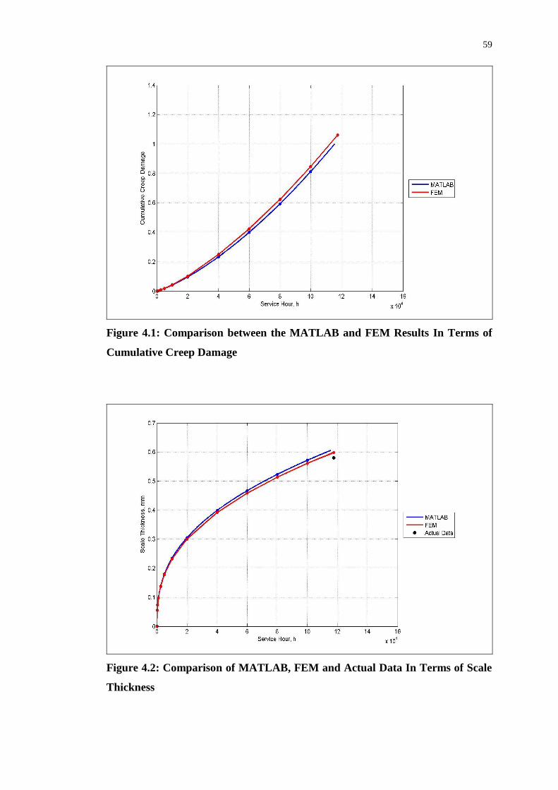
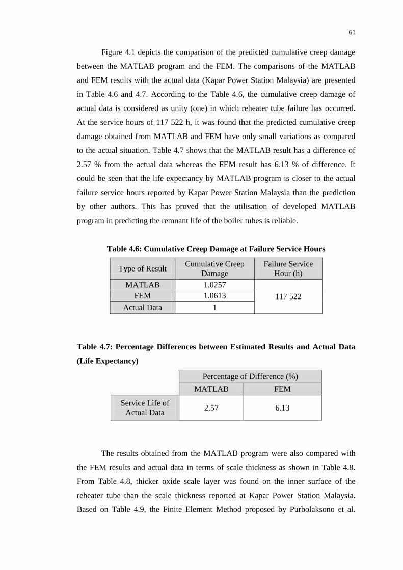
4.1 Validation of the Developed MATLAB Program 55
4.2 Evaluation of Constant B in Correlation Function 63
4.2.1 Tube Geometry 63
4.2.2 Steam Mass Flow Rate 66
4.2.3 Steam Temperature 68
4.2.4 Flue Gas Temperature 70
4.2.5 Summary 73
Page 9
ix
5 CONCLUSIONS AND RECOMMENDATIONS 74
5.1 Conclusions 74
5.2 Limitation of Developed MATLAB Program 76
5.3 Recommendations 76
REFERENCES 78
APPENDICES 81
Page 10
x
LIST OF TABLES
TABLE TITLE PAGE
3.1 Descriptions of Flow Chart Symbol Used 38
3.2 Input Parameters Required in Performing Analysis 47
3.3 Geometries of Tube 53
3.4 Models for Failure Analysis of Tube 54
3.5 Solid Material Properties for Boiler Tube 54
3.6 Parameters Required in Determining Gas Mass
Velocity, G 54
3.7 Compositions of Flue Gas at 15 % Air 54
4.1 Geometry, Service Time and Inner Scale
Thickness of the Tubes and the Year of Failure 56
4.2 Parameters Required in Determining Gas Mass
Velocity G 56
4.3 The Estimated Steam and Flue Gas Convection
Coefficients 56
4.4 Estimations of Scale Thickness and Cumulative
Creep Damage by MATLAB Program and Other
Authors (FEM) 57
4.5 Estimations of Average Temperature of Tube
Metal and Vickers Hardness by MATLAB
Program and Other Authors (FEM) 58
4.6 Cumulative Creep Damage at Failure Service
Hours 61
4.7 Percentage Differences between Estimated Results
and Actual Data (Life Expectancy) 61
Page 11
xi
4.8 Scale Thickness at Failure Service Hours 62
4.9 Percentage Differences between Estimate Results
and Actual Data (Scale Thickness) 62
4.10 Models Used for Tube Geometry Analysis 63
4.11 Generated Constant B and Average Percentage of
Difference In Terms of Tube Metal Temperature
(Model 1, 8, 9) 64
4.12 Models Used for Mass Flow Rate Analysis 66
4.13 Generated Constant B and Average Percentage of
Difference In Terms of Tube Metal Temperature
(Model 1, 2, 3) 66
4.14 Models Used for Steam Temperature Analysis 68
4.15 Generated Constant B and Average Percentage of
Difference In Terms of Tube Metal Temperature
(Model 1, 4, 5) 69
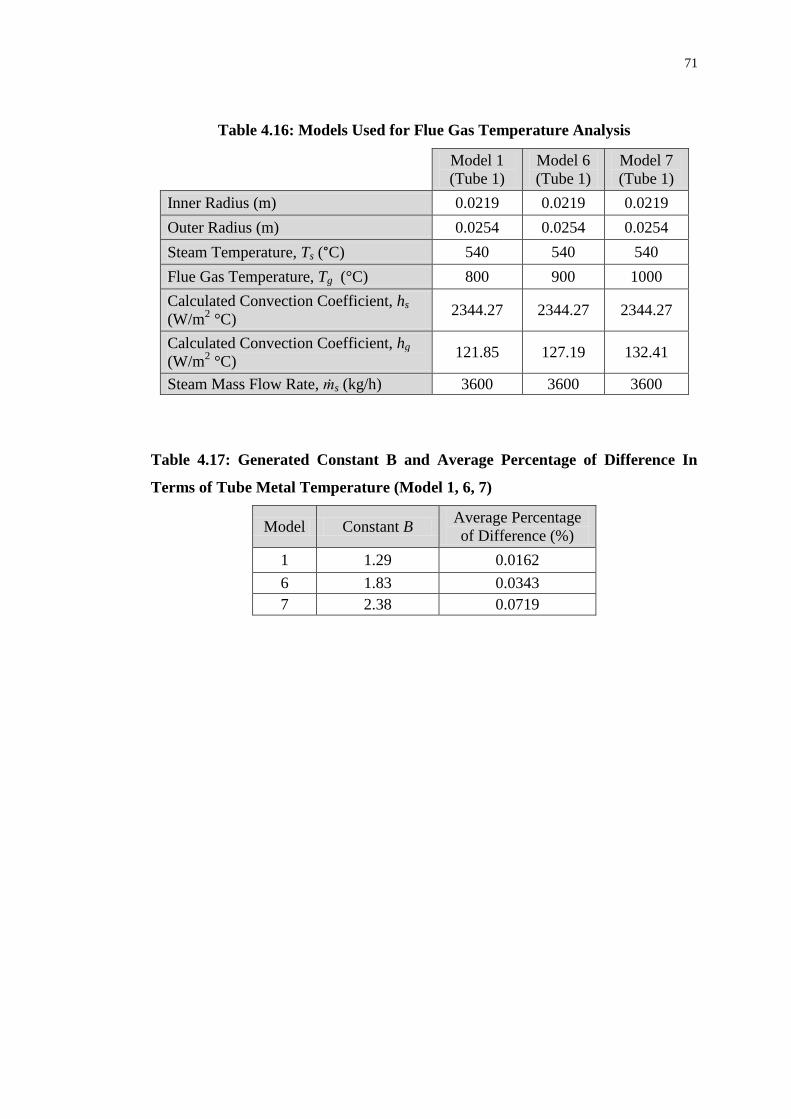
4.16 Models Used for Flue Gas Temperature Analysis 71
4.17 Generated Constant B and Average Percentage of
Difference In Terms of Tube Metal Temperature
(Model 1, 6, 7) 71
Page 12
xii
LIST OF FIGURES
FIGURE TITLE PAGE
2.1 Schematic Diagram of a Boiler (Prieto et al., 2006.
p. 187) 7
2.2 Microstructure of Creep Fracture Mechanisms
(Jones 2004. p. 878) 10
2.3 Intergranular Surface Cracks with the Creep Void
Evolution (Psyllaki, Pantazopoulos and Lefakis
2009. p. 1423) 11
2.4 Failure Due To Long Term Overheating (Lande et
al., 2011. p. 233) 11
2.5 Failure Due To Short Term Overheating (Lande et
al., 2011. p. 233) 13
2.6 Wall Thinning on the Fireside of the Tube
(Chandra, Kain and Dey 2011. p. 63) 15
2.7 Temperature Distribution of Boiler Tube Using
Simulation (Purbolaksono et al., 2010. p. 103) 16
2.8 Model of the Boiler Tubes with Oxide Scale
Formed On the Inner Surface (Purbolaksono et al.,
2010. p. 100) 18
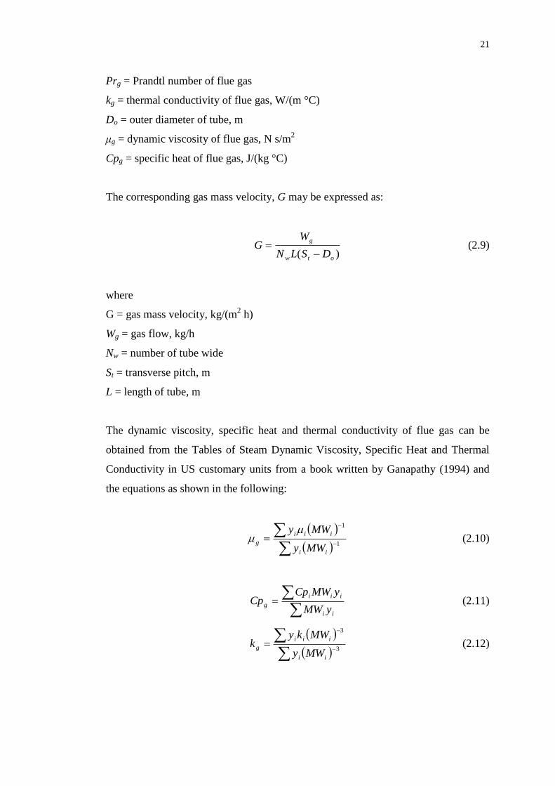
2.9 Inline and Staggered Arrangements of Bare Tubes
(Purbolaksono et al., 2010. p. 101) 22
2.10 Thermal Circuit of Superheater and Reheater
Tubes 23
2.11 Larson-Miller parameter diagram with stress
variation to rupture for 2.25Cr-1Mo steel (1 ksi =
6.895 MPa) (Smith 1971, cited in Purbolaksono et
al., 2010. p. 103) 27
Page 13
xiii
2.12 Steam-side scale formation for ferritic steels of 1-
3% chromium correlated with the Larson-Miller
parameter (Rehn et al., 1981, cited in
Purbolaksono et al., 2010. p. 101) 29
3.1 An Illustration of Usage of Off-page and On-page
Connectors 37
3.2 Flow Chart of Iterative Procedure (Part 1) 39
3.3 Flow Chart of Iterative Procedure (Part 2) 40
3.4 Flow Chart of Iterative Procedure (Part 3) 41
3.5 Flow Chart of Iterative Procedure (Part 4) 42
3.6 Flow Chart of Iterative Procedure (Part 5) 43
3.7 Flow Chart of Iterative Procedure (Part 6) 44
3.8 Flow Chart of Iterative Procedure (Part 7) 45
3.9 Prompt User to Decide in Overwriting Old Output
Data File 46
3.10 An Example of User Prompt in Command
Window 47
3.11 Illustration of Four Conditional Controls (Top) and
Three Conditional Controls (Bottom) 49
3.12 An Example of Summary of the Analysis 49
3.13 Part of the Results Displayed (Complete Iterations) 50
3.14 Part of the Results Displayed At Predetermined
Time Steps 50
3.15 Separate Function Files for Graph Plotting 51
4.1 Comparison between the MATLAB and FEM
Results In Terms of Cumulative Creep Damage 59
4.2 Comparison of MATLAB, FEM and Actual Data
In Terms of Scale Thickness 59
4.3 Comparison between the MATLAB and FEM
Results In Terms of Tube Metal Temperature 60
Page 14
xiv
4.4 Comparison between the MATLAB and FEM
Results In Terms of Vickers Hardness 60
4.5 Estimated Tube Metal Temperature with Different
Outer Radius (Tube) by Constant Estimation 65
4.6 Estimated Scale Thickness with Different Outer
Radius (Tube) 65
4.7 Estimated Tube Metal Temperature with Different
Steam Mass Flow Rate by Constant Estimation 67
4.8 Estimated Scale Thickness with Different Steam
Mass Flow Rate 67
4.9 Estimated Tube Metal Temperature with Different
Steam Temperature by Constant Estimation 69
4.10 Estimated Scale Thickness with Different Steam
Temperature 70
4.11 Estimated Tube Metal Temperature with Different
Flue Gas Temperature by Constant Estimation 72
4.12 Estimated Scale Thickness with Different Flue Gas
Temperature 72
Page 15
xv
LIST OF SYMBOLS / ABBREVIATIONS
B constant
Cp specific heat capacity, J/(kg °C)
D tube diameter, m
G gas mass velocity, kg/(m2 h)
HV Vickers hardness, HV
h convection coefficient, W/(m2 °C)
i gas constituent
I iteration
k thermal conductivity, W/(m °C)
L tube length, m
ṁ mass flow rate, kg/h
Nu Nusselt number
Nw number of tube wide
P Larson-Miller parameter
Pr Prandtl number
p operational internal pressure, MPa
R thermal resistance, °C/W
Re Reynolds number
r tube radius, m
St transverse pitch, m
t time, h
T temperature, °C
Wg gas flow, kg/h
X scale thickness, mm
y volume fraction
Page 16
xvi
µ dynamic viscosity, N s/m2
σh hoop stress, MPa
CCDMG cumulative creep damage
FEM finite element method
LMP Larson-Miller parameter
MW molecular weight
Page 17
xvii
LIST OF APPENDICES
APPENDIX TITLE PAGE
A MATLAB Program Codes (Main Program) 81
Page 18
CHAPTER 1
1 INTRODUCTION
1.1 Background of Boiler Tube
The purpose of boiler is to convert water into steam. The steam can be used for
various usages such as driving an engine to generate electricity, heating purpose and
for other industrial process applications. The boiler consists of several types, which
include water tube boiler, fire tube boiler, packaged boiler, fluidised bed combustion
(FBC) boiler, atmospheric fluidised bed combustion (AFBC) boiler and so forth. The
most popular boilers that used in many industries are water tube and fire tube boiler.
Water tube boiler is the one with water flowing through the tubes that enclosed in a
furnace heated externally while fire tube boiler comprises of fire or hot flue gas
directed through tubes surrounded by water.
Heat recovery steam generator (HRSG) is a good example of system in power
plant that utilises the boiler tube, typically a water tube boiler. In a combined cycle
gas turbine power plant, there are three major systems incorporated together, which
are gas turbine, steam turbine and HRSG. According to Ganapathy (2003), the
combined cycle plant incurs lower capital costs than the other power plants such as
conventional fossil power plants, and it is the most efficient electric generating
system available today.
The function of HRSG is to recover heat from the exhaust gas discharged
from the gas turbine and makes use of the heat energy to produce steam. The steam
produced will flow through steam turbine to generate electricity. Large numbers of
Page 19
2
HRSG systems are found in power generation plants due to its better efficiency
provided compared to the conventional fossil fired generating systems. A HRSG
system contains multiple of superheater and reheater tube units that are arranged in
parallel in which the pressurised steam flows through them. At the moment steam is
generated, it is in saturated form. Superheater and reheater tubes tend to raise the
steam temperature until it reaches superheated state and ready to be used in power
generation.
1.2 Problem Statement
In HRSG system, the steam flowing through the superheater and reheater tubes is
usually heated at a very high temperature to ensure that all saturated steam is
converted into superheated steam. In fact, the elevated temperature will cause the
formation of oxide scales on the inner surface of the tube. The oxide scale layer will
act as a thermal barrier and reduces the heat transfer from the hot flue gas into the
steam within the tube. As a result, the tube metal temperature rises due to the
accumulation of heat and reduced in cooling effect from steam. The metal tubes
experience excessive heat energy coupled with the deterioration of mechanical
properties of the tube alloy. The steam-carrying superheater and reheater tubes are
now subjected to potential failures such as creep rupture. The main concern here is
the consequence of failure of boiler tube can be expensive and tragic. Plant shutdown
as a result of tube failure can affect the entire operation of the power generation
system and pose financial losses. Therefore, a reliable estimation of the remaining
life of superheater and reheater tubes has become necessary for the power generation
plant boiler in reducing the tube failure rate as well as the cost by conducting life
assessment activities.
Page 20
3
1.3 Aim and Objectives
The ultimate goal of the research is to develop a reliable program that can perform
iterative procedure for the purpose of estimating the oxide scale thickness formed,
wall thinning, hardness, hoop stress, heat flux of the tube, and the remaining life of
superheater and reheater tubes. The objectives of the project are:
1) To propose an iterative analytical procedure that can be used to investigate
the integrity of boiler tubes such as oxide scale thickness, hardness, heat flux,
hoop stress, wall thinning and the remaining life.
2) To develop a reliable program in MATLAB based on the proposed iterative
analytical procedure.
3) To determine and investigate the correlation functions of oxide scale growth
and temperature increase at various operating conditions using iterative
analytical procedure.
1.4 Scope of the Research
In this project, an iterative analytical procedure has been proposed to perform various
analyses and studies on the boiler tube. The iterative procedure tends to predict the
remnant life of the boiler tube under an operating condition and analyse the
performance characteristics of boiler tubes in terms of oxide scale thickness,
hardness, heat flux, hoop stress and wall thinning. These performance characteristics
are as functions of temperature and time. Since the project was only based on simple
model analysis, all the parameters such as oxide scale thickness, heat flux and so
forth were analysed in one dimension. For instance, the oxide scale was treated to be
uniformly grown with constant increment in thickness of oxide layer rather than
considering the oxide layer that covers a surface area (two dimensions).
Page 21
4
A detailed flow chart was established before implementing the iterative
procedure in MATLAB. The results obtained from the MATLAB program was
compared with the work done by other authors and the actual data reported at Kapar
Power Station Malaysia. The validation of the MATLAB results is important as it
evaluates the reliability of the MATLAB program if the results may be used to assist
in preventive maintenance of boiler tube in power plant. It is capable to perform
various tasks such as graph potting and boiler tube life prediction that incorporates
the thinning effect as well as other parameters. It can also be used to investigate the
correlation function between the oxide scale thickness and temperature change in
order to meet the objectives of the research.
The prediction of temperature increase in boiler tube was demonstrated by
utilising a generated constant B that correlating the scale oxide thickness and tube
metal temperature change. A few sets of relevant parameters were presented and
used to study the constant estimation method in predicting the temperature increase
in tube. The prediction using a constant B could be used to support the condition
monitoring of boiler tubes in power plants.
1.5 Structure of Thesis
All the literature reviews related to this project are discussed in Chapter 2. This
chapter starts with an introduction of the types of boiler tubes operated in power
plant. The damages or failures in relative to the boiler tubes are explained and the
researches done by other authors in those relevant topics are reviewed and discussed.
The later part is the evaluation on the methods used by other authors in the prediction
of oxide scale growth following by the fundamental of heat transfer for boiler tube
analysis. This section is mainly discussed on the heat transfer-related equations and
principles.
Chapter 3 describes the methodology that employed in order to achieve the
aims and objectives of this project. The proposed analytical iterative procedure is
explained in steps. A detailed flow chart that implements the iterative procedure in
Page 22
5
MATLAB is presented. Further explanations of the development of the MATLAB
program are discussed. Next, a method in estimating a constant correlating the
temperature increase and scale thickness is proposed.
Chapter 4 discusses the results obtained from the MATLAB and the
comparison between the estimated results with the work carried out by other authors
and the actual data from one of the power stations in Malaysia. The effects of the
changes in several parameters to the correlation function between temperature
change and scale growth are investigated.
Chapter 5 explains the conclusions that can be draw from the findings in this
project. Limitations of the developed MATLAB program are briefly explained and
two recommendations for improvement of this project are suggested.
Page 23
CHAPTER 2
2 LITERATURE REVIEW
2.1 Description of Heat Recovery Steam Generator (HRSG)
Figure 2.1 illustrates a schematic diagram of a boiler for HRSG system. The relevant
components in the boiler tube are labelled accordingly. An understanding of the
structure and the operation of the water tube boiler (HRSG) is required beforehand.
The mechanism in the boiler begins with the combustion that takes place in the
furnace. The fuel can be coal, oil or natural gas. The gases produced from the
combustion travels up to the roof of the furnace and at the same time, convert the
water inside the water wall tubes into steam. The hot flue gases follow the channel of
the furnace and flow across the secondary superheater and reheater tubes and primary
reheater tubes bank. Then, the gases flow downward and pass through the sections of
primary superheater and economiser. Before the exhaust gases are discharged, they
undergo heating process in the air preheater and also a series of cleaning processes
using various devices. The dash arrows depict the flow of the combustion gases
throughout the boiler.
Page 24
7
Figure 2.1: Schematic Diagram of a Boiler (Prieto et al., 2006. p. 187)
The boiler tubes can be divided into two separated fluid flows. The hot flue
gases flow path involves the region at the fireside of the boiler tubes from the water
wall tubes until the economiser. On the other hand, the flow of the steam and water is
along the water-side of the boiler tubes. The water-side of the boiler tubes include the
passages that are in dash lines as shown in Figure 2.1.
Many water tube boilers are of natural water circulation. In natural circulation
systems, a steam-water separation equipment or known as drum is required to
separate the steam and water and the circulation of water is by convection currents.
Natural circulation is the result of density difference whereby the colder and denser
fluid (water) is circulated from the drum to downcomer situated at the outside of
furnace while the hotter and less dense fluid (steam) is delivered to the superheater
and the high-pressure section of the turbine inlet. The steam discharged from the
low-pressure section of turbine is then returned to the reheater unit. The low-pressure
steam is then condensed into feedwater through condenser, feedwater heaters and
Page 25
8
deaerators. Later, the feedwater is fed into the economizer and heated before it enters
the water wall tubes.
Another type of water circulation is called forced once through circulation.
The difference of the forced once through circulation compared to the natural
circulation is that the water and steam is moved by pump. Besides that, the forced
once through design does not have recirculation via drums and circulating pumps as
in the natural circulation. Forced once through circulation is of advantage when the
pressure is very high. If the pressure is very high, the density difference between the
water and steam is very less, in which natural circulation is not favourable (Grote &
Antonsson 2009).
The superheater and reheater consist of heat-absorbing surface that raises the
steam temperature above its saturation point. One of the reasons behind for doing
this is due to the elimination of the moisture or water vapour before it enters the
turbine. Corrosion of the turbine components such as turbine blades results from the
chemical reaction between the water vapour and the metallic surfaces. Another
reason is the thermodynamic gain in efficiency.
2.2 Damage Mechanisms on Superheater and Reheater Tube
The superheater and reheater tubes in the boiler power plants are most likely to
expose to a series of problems that can easily lead to tube failure at high temperature.
Generally the problems can be divided into two categories, which are corrosion
related problems and mechanical related problems. The typical mechanical related
problems are creep fracture and overheating while corrosion related problems
encountered in superheater and reheater tube is fireside corrosion. There are many
else of failures occur in different components of boiler tube. However, merely few
failures that have highlighted are of interest in this research.
Page 26
9
2.2.1 Creep
The major damage mechanism in most of the power generation plants is due to creep
damage. Creep is a type of time-dependent deformation that occurs under stress and
elevated temperature. Failure that caused by creep is known as creep rupture or stress
rupture. Creep rupture is often happened to be the final stage of failure in boiler tubes.
According to the statistics reported by Jones (2004), approximately 10 % of all
power plant breakdowns are resulted due to creep failures happened in boiler tubes.
Some problems associated with creep rupture can be related to the high temperature
exposure such as long term overheating and short term overheating, and each will be
further discussed in the following subsections.
Jones (2004) described three basic mechanisms of creep rupture, which are
intergranular creep facture, transgranular creep fracture and dynamic recrystallisation.
Intergranular creep fracture is more likely to happen at low stresses in the ductile
boiler tubes. Voids will nucleate at the grain boundaries under the applied tensile
stress and leads to the growth of defects. Eventually the deformation is concentrated
at the grain boundaries with small reduction in area and ductility and breaks later.
Transgranular creep fracture tends to occur at high stresses. Similarly, the voids
nucleate and propagate throughout the grains. However, the tensile ductility and
reduction in fracture area are much greater than the intergranular creep failure. At the
combination of high temperatures and stresses, dynamic recrystallisation probably
will occur in which waves of recrystallisation pass through the creeping material and
eliminate the microstructural damaged resulted from the formation of creep. Thus,
voids will not nucleate as how will be happened in the other two fractures and the
round bar metal tubes will break down to a point and failure.
Page 27
10
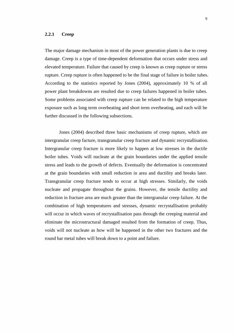
Figure 2.2: Microstructure of Creep Fracture Mechanisms (Jones 2004. p. 878)
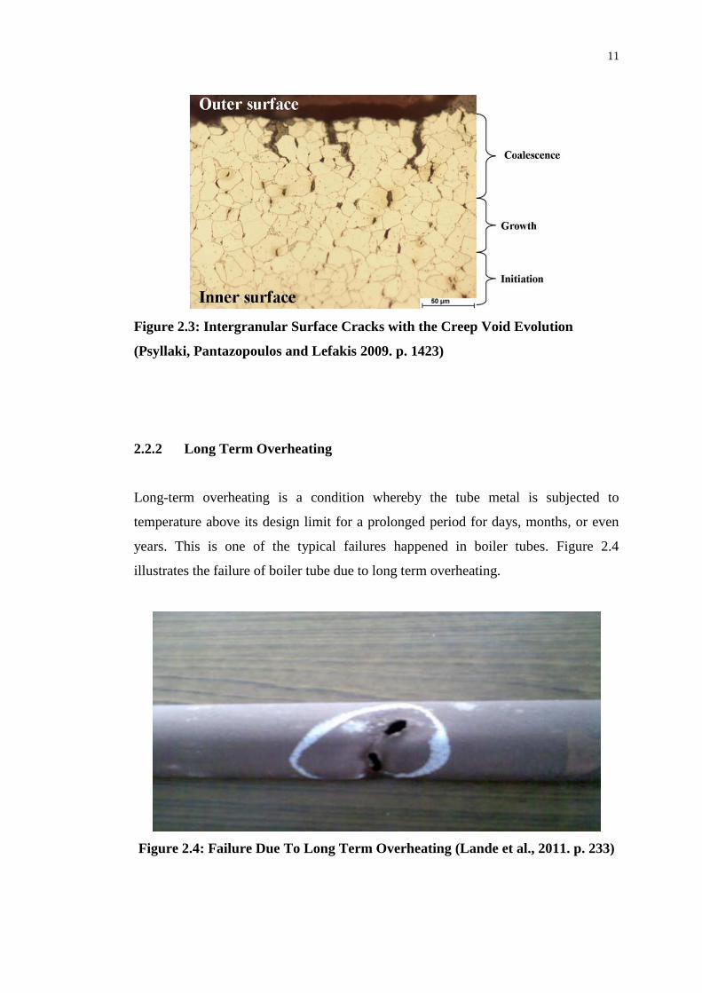
In the investigation carried out by Psyllaki, Pantazopoulos and Lefakis (2009),
creep void evolution was found in the creep-failed boiler tube. Psyllaki,
Pantazopoulos and Lefakis (2009) observed that the void coalescence (final stage in
the failure of ductile materials) that filled with oxidation compositions resulted in
intergranular surface cracks at the outside surface of the boiler tube. As a result, a
zone of creep void growth was found across the tube wall. On the other hand, an
initiation of individual voids was found along the grain boundaries towards the inner
surface of the tube wall. This phenomenon (initiation, growth and coalescence)
showed a temperature gradient across the tube wall at which the heat transfer
between the combustion gases at the external surface of the boiler tube and the
pressurised steam flow in the inner surface of the tube took place.
Page 28
11
Figure 2.3: Intergranular Surface Cracks with the Creep Void Evolution
(Psyllaki, Pantazopoulos and Lefakis 2009. p. 1423)
2.2.2 Long Term Overheating
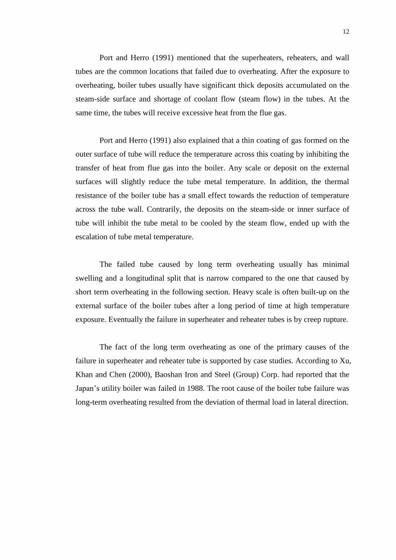
Long-term overheating is a condition whereby the tube metal is subjected to
temperature above its design limit for a prolonged period for days, months, or even
years. This is one of the typical failures happened in boiler tubes. Figure 2.4
illustrates the failure of boiler tube due to long term overheating.
Figure 2.4: Failure Due To Long Term Overheating (Lande et al., 2011. p. 233)
Page 29
12
Port and Herro (1991) mentioned that the superheaters, reheaters, and wall
tubes are the common locations that failed due to overheating. After the exposure to
overheating, boiler tubes usually have significant thick deposits accumulated on the
steam-side surface and shortage of coolant flow (steam flow) in the tubes. At the
same time, the tubes will receive excessive heat from the flue gas.
Port and Herro (1991) also explained that a thin coating of gas formed on the
outer surface of tube will reduce the temperature across this coating by inhibiting the
transfer of heat from flue gas into the boiler. Any scale or deposit on the external
surfaces will slightly reduce the tube metal temperature. In addition, the thermal
resistance of the boiler tube has a small effect towards the reduction of temperature
across the tube wall. Contrarily, the deposits on the steam-side or inner surface of
tube will inhibit the tube metal to be cooled by the steam flow, ended up with the
escalation of tube metal temperature.
The failed tube caused by long term overheating usually has minimal
swelling and a longitudinal split that is narrow compared to the one that caused by
short term overheating in the following section. Heavy scale is often built-up on the
external surface of the boiler tubes after a long period of time at high temperature
exposure. Eventually the failure in superheater and reheater tubes is by creep rupture.
The fact of the long term overheating as one of the primary causes of the
failure in superheater and reheater tube is supported by case studies. According to Xu,
Khan and Chen (2000), Baoshan Iron and Steel (Group) Corp. had reported that the
Japan’s utility boiler was failed in 1988. The root cause of the boiler tube failure was
long-term overheating resulted from the deviation of thermal load in lateral direction.
Page 30
13
2.2.3 Short Term Overheating
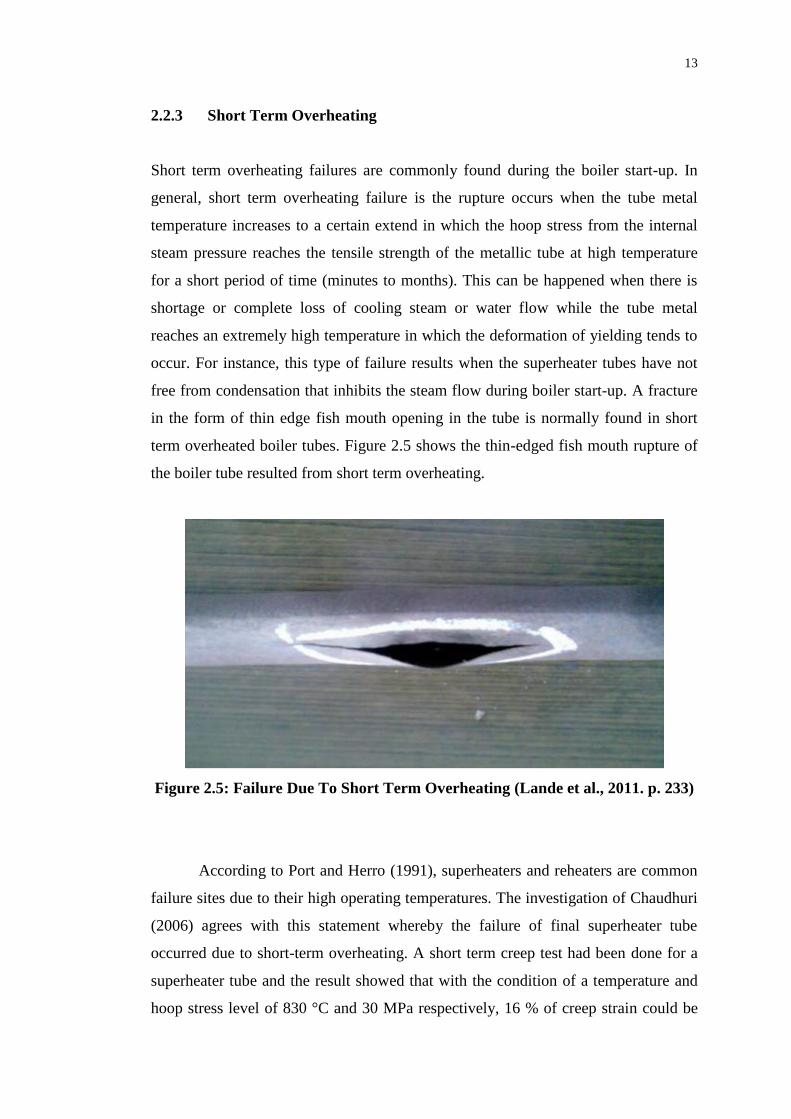
Short term overheating failures are commonly found during the boiler start-up. In
general, short term overheating failure is the rupture occurs when the tube metal
temperature increases to a certain extend in which the hoop stress from the internal
steam pressure reaches the tensile strength of the metallic tube at high temperature
for a short period of time (minutes to months). This can be happened when there is
shortage or complete loss of cooling steam or water flow while the tube metal
reaches an extremely high temperature in which the deformation of yielding tends to
occur. For instance, this type of failure results when the superheater tubes have not
free from condensation that inhibits the steam flow during boiler start-up. A fracture
in the form of thin edge fish mouth opening in the tube is normally found in short
term overheated boiler tubes. Figure 2.5 shows the thin-edged fish mouth rupture of
the boiler tube resulted from short term overheating.
Figure 2.5: Failure Due To Short Term Overheating (Lande et al., 2011. p. 233)
According to Port and Herro (1991), superheaters and reheaters are common
failure sites due to their high operating temperatures. The investigation of Chaudhuri
(2006) agrees with this statement whereby the failure of final superheater tube
occurred due to short-term overheating. A short term creep test had been done for a
superheater tube and the result showed that with the condition of a temperature and
hoop stress level of 830 °C and 30 MPa respectively, 16 % of creep strain could be
Page 31
14
found within 2 h. This proved that the boiler tube will fail as a result of short term
overheating when the temperature reaches 830 °C.
2.2.4 Fireside Erosion-Corrosion and Wall Thinning
Fireside corrosion and erosion is one of the damage mechanisms that tends to occur
on the outer surface of the superheater and reheater tubes and may result in wall
thinning over prolonged time. As the name implies, it is a combined corrosion and
erosion processes. The fireside corrosion may defined as material wastage by the
chemical reaction between the tube metal and the surrounding environment at high
temperature and erosion may be define as the mechanically surface material removal
by the abrasive of moving fluid interacting with the metallic surface. In short, this
damage mechanism is promoted by the elevated operational temperature and high
velocity of fluid or flue gas.
Hernas et al. (2004) has reported that the fireside erosion-corrosion of boiler
tube is as a result of corrosive atmosphere or environment containing a composition
of sulphur and chlorine compounds. Chaudhuri (2006) also found the presence of
other corrosive elements such as potassium, calcium and silicon from the detriment
of the outer surface of a failed reheater tube based on an extensive analysis. A
research (Li et al., 2007) showed the high temperature fireside corrosion and erosion
has led to the wall thinning of the superheater tube and the formation of two-layer
corrosion scales: an inner layer of sulphur compound and an outer layer of oxide
scales. This finding was supported by the research done by Chandra, Kain and Dey
(2011). In addition, the deposition of calcium sulphate on the superheater tubes
(carbon steel grade SA213-T22 or 2.25Cr-1Mo) and its spallation were repeatedly
enhanced by each other, causing the reduction of tube wall thickness that was
believed to be the main cause of the tube failure. The boiler tube failure associated
with the fireside erosion-corrosion could be happened by the mean of either thinning
of wall or formation of cracks, and eventually ended up with fatigue (Syed, Simms
and Oakey 2012) or increase in hoop stress (Vikrant et al., 2013).
Page 32
15
Figure 2.6: Wall Thinning on the Fireside of the Tube (Chandra, Kain and Dey
2011. p. 63)
Thus, the researches done in the past proved that wall thinning effect is one of
the crucial factors to be considered in evaluating the boiler tube failures. Preventive
steps can be taken to curb and alleviate the corrosion-related problems, ensuring a
longer life span of the tube to be possible.
2.3 Prediction on Oxide Scale Growth
Oxide scales in the boiler tubes resulting from the prolonged exposure of elevated
temperature can be determined by multiple types of analysis approach. A
methodology using calculation, non-destructive and destructive evaluations to help in
life prediction of boiler tubes was developed by Electric Power Research Institute
(EPRI) and its contractors (Viswanathan et al., 1994). The thickest steam-side oxide
scale in the tubes is identified and measured by using ultrasonic technique based on
Page 33
16
the methodology. Further researches were done such as the validation of the
ultrasonic technique in measuring scale and the identification of the appropriate
stress formula and oxide growth laws.
Purbolaksono et al. (2009c) has proposed a technique for the estimation of the
oxide scale thickness in superheater and reheater tube by using empirical formula
and finite element modelling (FEM) simulation using ANSYS. The oxide scale
thickness was found to be influenced by heat transfer parameters including the
temperature of steam and flue gas, convection coefficients on the outer surface of
tube and mass flow rates of steam. The computer simulation generated the
temperature distribution of the superheater and reheater tube wall and illustrated the
correlation between the scale thickness and the metal tube temperature. Purbolaksono
et al. (2010) further on the research by incorporating the iterative procedure and
evaluated two failure cases in superheater and reheater tubes. The results obtained
were shown to be in good conformity with the actual data.
Figure 2.7: Temperature Distribution of Boiler Tube Using Simulation
(Purbolaksono et al., 2010. p. 103)
Page 34
17
2.4 Fundamental of Heat Transfer for Boiler Tube Analysis
The operation of the superheater and reheater tube involves the exchange of heat
between the high pressure steam in contact with the internal surface of tube wall and
the hot flue gas in contact with the outer surface of tube wall. Before any analysis on
the boiler tube can be performed, one should have fundamental knowledge in heat
transfer theory. Heat transfer is defined as thermal energy in transit due to a spatial
temperature difference (Incropera et al., 2007). Heat transfer mechanism can be
divided into three categories: conduction, convection and radiation.
Conduction process occurs when a temperature gradient exists between
substances that are in direct contact with each other. The medium of conduction
process may be a solid or a fluid. The heat transfer that occurs between a surface and
a moving fluid at which both are at different temperatures is known as convection.
Convection is the up and down movement of fluid (gas or liquid) caused by the
thermal energy transmission. In a vacuum or empty space, heat transfer is also
achievable. All surfaces of finite temperature emit energy in the form of
electromagnetic waves. The electromagnetic waves travel through the space even in
the absence of medium. This type of heat transfer is called radiation.
In this research, merely conduction and convection processes are of the
interest and the radiation effect is assumed to be absent. The heat transfer across the
water boiler tube wall is in the form of conduction while the heat transfer at the
steam-tube interface and gas-tube interface are through convection.
A model that represents the steady state heat transfer taking place in
superheater and reheater tubes is illustrated in Figure 2.8. The model indicating the
tube metal wall is divided into two regions, which are scale region and tube region.
Scale region is located at the inner surface of tube wall that is in contact with the
steam region. This oxide scale is usually a duplex (inner spinel layer and outer
magnetite layer) or triplex (inner spinel layer, middle magnetite layer and outer
hematite layer) (Purbolaksono et al., 2009c). However, the material of scale is treated
as all magnetite (Fe3O4) for the ease of analysis in this research.
Page 35
18
Figure 2.8: Model of the Boiler Tubes with Oxide Scale Formed On the Inner
Surface (Purbolaksono et al., 2010. p. 100)
2.4.1 Convection Coefficient of Steam, hs
The steam inside the superheater and reheater tubes is treated as a fully developed
turbulent flow along the circular tube. The heat transfer inside the boiler tube is
considered as an internal forced convection with turbulent flow. Thus, the Nusselt
number of the steam can be computed using the Dittus-Boelter equation:
4.08.00023.0 sss rPeRNu (2.1)
where Res is the Reynolds number of steam and the Prs is the Prandtl number of
steam that can be expressed as:
si
ss
D
meR
900
(2.2)
Page 36
19
s
ss
sk
CprP
(2.3)
where
Nus = Nusselt number of steam
Res = Reynolds number of steam
Prs = Prandtl number of steam
sm = mass flow rate of steam, kg/h
Di = inner diameter of tube, m
μs = dynamic viscosity of steam, N s/m2
Cps = specific heat of steam, J/(kg °C)
ks = thermal conductivity of steam, W/(m °C)
In order to obtain the values for dynamics viscosity, specific heat and thermal
conductivity of steam, operating steam temperature (in degrees Fahrenheit) and
pressure (in psi) are required. The values for dynamic viscosity μs, specific heat Cps
and thermal conductivity ks of the steam are extracted from the Tables of Steam
Dynamic Viscosity, Specific Heat and Thermal Conductivity (Ganapathy 2003) in
US customary unit.
The Equation 2.1 must comply with the following conditions (Incropera et al., 2007):
I) 0.7 < Pr < 160
II) Re > 10 000
III) D
L> 10; where L is the length of tube, m
IV) All fluid properties are evaluated at mean temperature, Tm.
Since
s
iss
k
DLhNu
)( (2.4)
Page 37
20
the steam convection coefficient for fully developed turbulent flow in circular tube is
obtained by rearranging the Equation 2.4:
4.08.00023.0)( ss
i
s
s rPeRD
kLh (2.5)
where
hs = convection coefficient of steam, W/(m2 °C)
2.4.2 Convection Coefficient of Flue Gas, hg
The heat transfer of the hot flue gas outside the boiler tube is treated as external
forced convection as a result of cross flow of the flue gas over the superheater and
reheater tubes. A conservative estimate of convection coefficient of flue gas, hg for
the flow of flue gas over the bare tubes in inline and staggered arrangements (see
Figure 2.9) is expressed as (Ganapathy 2003):
33.06.033.0 gg
o
g
g rPeRD
kh (2.6)
and the Reynolds and Prandtl numbers of flue gas may be expressed as:
g
og
GDeR
3600 (2.7)
g
gg
gk
CprP
(2.8)
where
hg = convection coefficient of flue gas, W/(m2 °C)
Reg = Reynolds number of flue gas
Page 38
21
Prg = Prandtl number of flue gas
kg = thermal conductivity of flue gas, W/(m °C)
Do = outer diameter of tube, m
μg = dynamic viscosity of flue gas, N s/m2
Cpg = specific heat of flue gas, J/(kg °C)
The corresponding gas mass velocity, G may be expressed as:
)( otw
g
DSLN
WG
(2.9)
where
G = gas mass velocity, kg/(m2 h)
Wg = gas flow, kg/h
Nw = number of tube wide
St = transverse pitch, m
L = length of tube, m
The dynamic viscosity, specific heat and thermal conductivity of flue gas can be
obtained from the Tables of Steam Dynamic Viscosity, Specific Heat and Thermal
Conductivity in US customary units from a book written by Ganapathy (1994) and
the equations as shown in the following:
1
1
ii
iii
gMWy
MWy (2.10)
ii
iii
gyMW
yMWCpCp (2.11)
3
3
ii
iii
gMWy
MWkyk (2.12)
Page 39
22
where
MW = molecular weight
y = volume fraction
i = gas constituent
Figure 2.9: Inline and Staggered Arrangements of Bare Tubes (Purbolaksono et
al., 2010. p. 101)
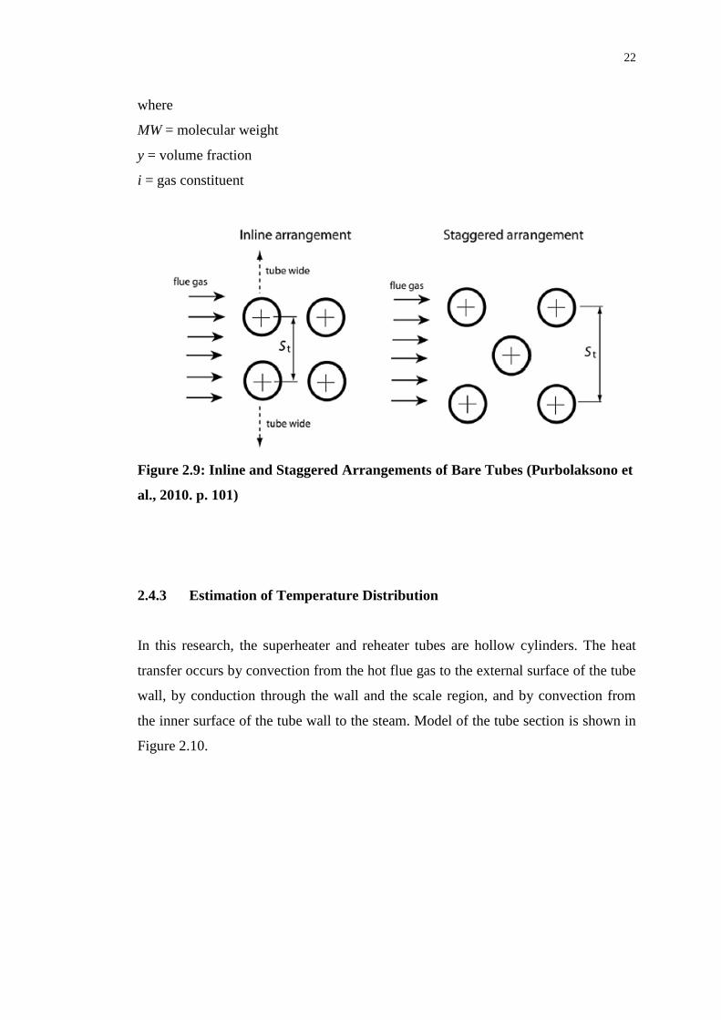
2.4.3 Estimation of Temperature Distribution
In this research, the superheater and reheater tubes are hollow cylinders. The heat
transfer occurs by convection from the hot flue gas to the external surface of the tube
wall, by conduction through the wall and the scale region, and by convection from
the inner surface of the tube wall to the steam. Model of the tube section is shown in
Figure 2.10.
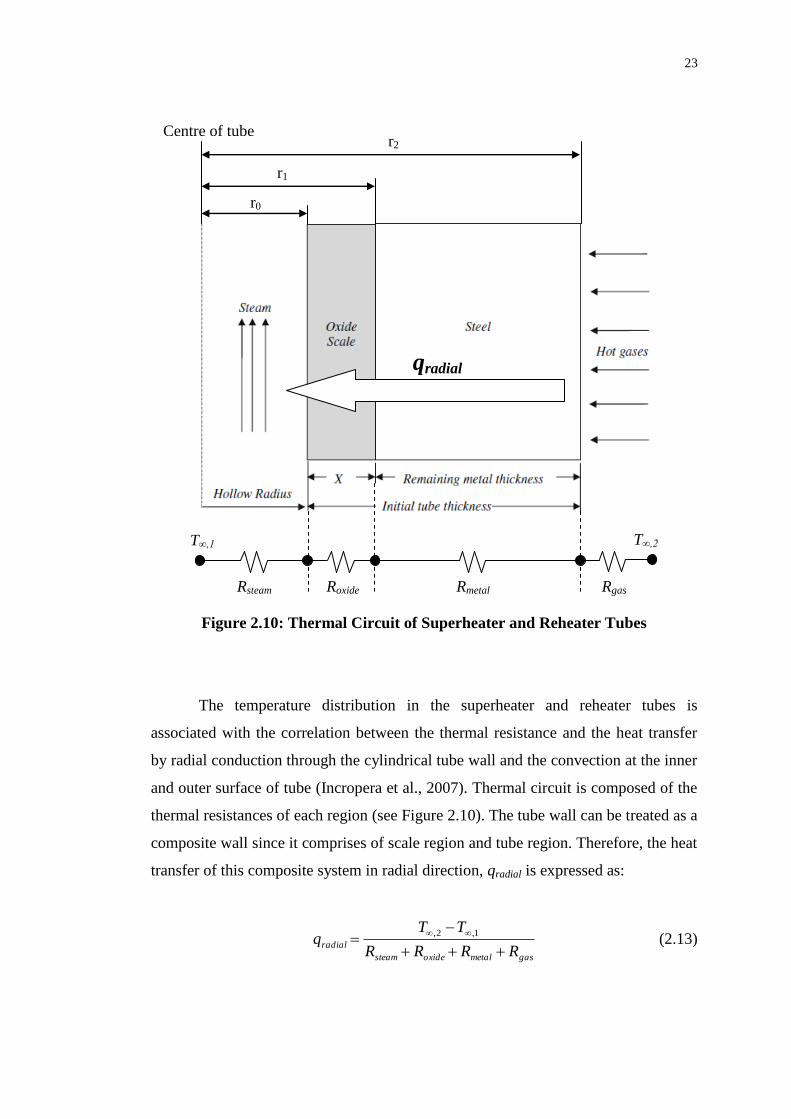
Page 40
23
Figure 2.10: Thermal Circuit of Superheater and Reheater Tubes
The temperature distribution in the superheater and reheater tubes is
associated with the correlation between the thermal resistance and the heat transfer
by radial conduction through the cylindrical tube wall and the convection at the inner
and outer surface of tube (Incropera et al., 2007). Thermal circuit is composed of the
thermal resistances of each region (see Figure 2.10). The tube wall can be treated as a
composite wall since it comprises of scale region and tube region. Therefore, the heat
transfer of this composite system in radial direction, qradial is expressed as:
gasmetaloxidesteam
radialRRRR
TTq
1,2, (2.13)
r0
r1
r2 Centre of tube
Rsteam Roxide Rmetal Rgas
T∞,1 T∞,2
qradial
Page 41
24
in which
Lrh
Rs
steam
02
1
(2.14)
Lk
rrnlR
oxide
oxide2
)/( 01 (2.15)
Lk
rrnlR
metal
metal2
)/( 12 (2.16)
Lrh
Rg
gas
22
1
(2.17)
where
Rsteam = thermal resistance of steam, °C/W
Roxide = thermal resistance of oxide, °C/W
Rmetal = thermal resistance of metal, °C/W
Rgas = thermal resistance of flue gas, °C/W
T∞,1 = temperature of steam, °C
T∞,2 = temperature of flue gas, °C
hs = convection coefficient of steam, W/(m2 °C)
hg = convection coefficient of flue gas, W/(m2 °C)
koxide = thermal conductivity of oxide scale, W/(m °C)
kmetal = thermal conductivity of tube metal, W/(m °C)
r0 = radius up to inner surface of tube, m
r1 = radius up to oxide scale surface of tube, m
r2 = radius up to outer surface of tube, m
L = length of tube, m
Page 42
25
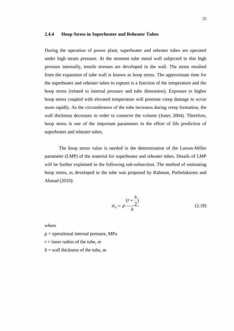
2.4.4 Hoop Stress in Superheater and Reheater Tubes
During the operation of power plant, superheater and reheater tubes are operated
under high steam pressure. At the moment tube metal wall subjected to this high
pressure internally, tensile stresses are developed in the wall. The stress resulted
from the expansion of tube wall is known as hoop stress. The approximate time for
the superheater and reheater tubes to rupture is a function of the temperature and the
hoop stress (related to internal pressure and tube dimension). Exposure to higher
hoop stress coupled with elevated temperature will promote creep damage to occur
more rapidly. As the circumference of the tube increases during creep formation, the
wall thickness decreases in order to conserve the volume (Jones 2004). Therefore,
hoop stress is one of the important parameters in the effort of life prediction of
superheater and reheater tubes.
The hoop stress value is needed in the determination of the Larson-Miller
parameter (LMP) of the material for superheater and reheater tubes. Details of LMP
will be further explained in the following sub-subsection. The method of estimating
hoop stress, σh developed in the tube was proposed by Rahman, Purbolaksono and
Ahmad (2010):
h
hr
ph
)2
(
(2.18)
where
p = operational internal pressure, MPa
r = inner radius of the tube, m
h = wall thickness of the tube, m
Page 43
26
2.4.5 Larson-Miller Parameter
Life assessment of superheater and reheater tube can be conducted by estimating the
oxide scale thickness on the inner surface of tube wall. As the superheater and
reheater are placed in service, oxide scale gradually grows on the tube wall and the
tube metal temperature increases with respect to the time. Eventually, the creep
rupture occurs due to high hoop stress in the tube wall.
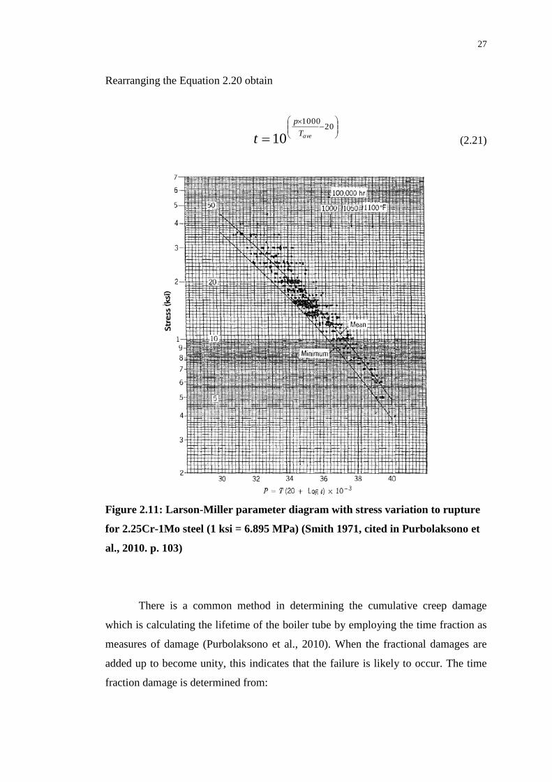
According to Ganapathy (2003), creep data are available for different
materials in the form of the LMP. This relates the value of rupture stress to the
temperature, T in degrees Rankine (degrees Fahrenheit + 460) and the remaining
lifetime t, in hours.
)log20( tTLMP (2.19)
Before estimating the remaining life of the superheater and reheater tube, the
hoop stress, σh calculated from the Equation 2.18 is utilised in order to determine the
LMP value from a diagram of LMP.
Every material has its own LMP chart. Figure 2.11 shows a LMP diagram for
annealed material 2.25Cr-1Mo steel (or SA213-T22 steel) with a mean curve
correlating the stress variation and the LMP value. Based on Figure 2.11, the
equation of Larson-Miller parameter can be expressed in another form:
1000
)log20( tTLMP ave
(2.20)
where
Tave = average temperature of tube metal, °Ra
t = rupture time, h
Page 44
27
Rearranging the Equation 2.20 obtain
20
1000
10 aveT
p
t (2.21)
Figure 2.11: Larson-Miller parameter diagram with stress variation to rupture
for 2.25Cr-1Mo steel (1 ksi = 6.895 MPa) (Smith 1971, cited in Purbolaksono et
al., 2010. p. 103)
There is a common method in determining the cumulative creep damage
which is calculating the lifetime of the boiler tube by employing the time fraction as
measures of damage (Purbolaksono et al., 2010). When the fractional damages are
added up to become unity, this indicates that the failure is likely to occur. The time
fraction damage is determined from:
Page 45
28
1ri
si
t
t (2.22)
where
tsi = service time, h
tri = rupture time, h
The rupture time is obtained from Equation 2.21 while the service time refers
to the service life of superheater and reheater tubes. By knowing the LMP and the
average tube metal temperature, the remaining life of the superheater and reheater
can be estimated.
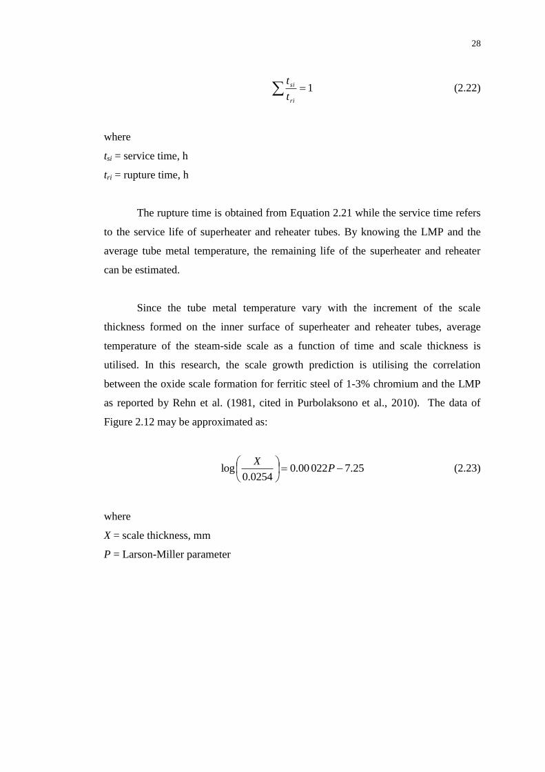
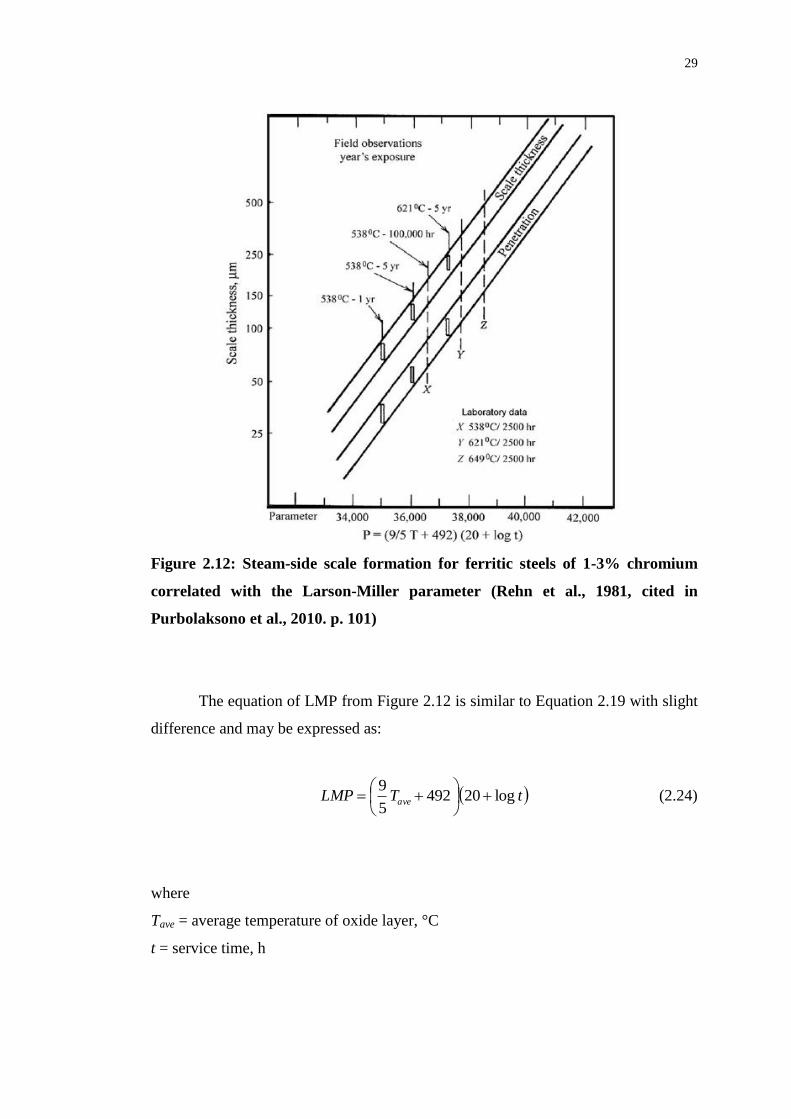
Since the tube metal temperature vary with the increment of the scale
thickness formed on the inner surface of superheater and reheater tubes, average
temperature of the steam-side scale as a function of time and scale thickness is
utilised. In this research, the scale growth prediction is utilising the correlation
between the oxide scale formation for ferritic steel of 1-3% chromium and the LMP
as reported by Rehn et al. (1981, cited in Purbolaksono et al., 2010). The data of
Figure 2.12 may be approximated as:
25.702200.00254.0
log
P
X (2.23)
where
X = scale thickness, mm
P = Larson-Miller parameter
Page 46
29
Figure 2.12: Steam-side scale formation for ferritic steels of 1-3% chromium
correlated with the Larson-Miller parameter (Rehn et al., 1981, cited in
Purbolaksono et al., 2010. p. 101)
The equation of LMP from Figure 2.12 is similar to Equation 2.19 with slight
difference and may be expressed as:
tTLMP ave log204925
9
(2.24)
where
Tave = average temperature of oxide layer, °C
t = service time, h
Page 47
30
2.4.6 Vickers Hardness
Hardness of the superheater or reheater tube is influenced after a long operation time
with the continuous increasing temperature. In other words, the strength of the tube
will deteriorate over long term exposure to the operating temperature. A soften tube
poses a risk in the occurrence of rupture in the tube. This can lead to the tube burst as
a result of inability to withstand the high pressure inside the tube. Therefore, the
hardness of the superheater and reheater tube is examined and evaluated in line with
the life assessment of the tube.
An equation that correlates the Vickers hardness and the Larson-Miller
parameter for 2.25Cr-1Mo steel under as-quenched condition may be expressed as
(Viswanathan 1993):
PHVHardness 020669.0713.961)( (2.25)
where
P = Larson-Miller parameter
HV = Vickers hardness, HV
2.4.7 Heat Flux
Heat flux is directly linked to the thermal efficiency of the superheater and reheater
tube. It is the heat transfer rate across a surface area of the tube. The escalation of the
temperature coupled with the oxide scale layer of the tube tends to impede the heat
transfer to take place. Therefore, a decline heat flux indicates that less heat energy is
being transferred from the flue gas to the steam (Purbolaksono et al., 2009a). This
feature is usually utilised to measure the thermal efficiency in conjunction with the
prediction of remaining life of superheater and reheater tube.
Page 48
31
The distribution of heat flux at all locations of the tube can be determined
from the principle of heat flux by conduction at cylindrical wall and heat flux by
convection at a surface. In this study, the heat flux distribution is divided into four
regions, which are heat flux at inner surface, outer surface, oxide scale layer and tube
metal wall of the tube.
The heat flux by conduction is obtained from the temperature difference
across the tube wall with the thermal conductivity of the solid material whereas the
heat flux by convection is determined from the temperature difference between the
steam and the inner surface (or flue gas and the outer surface) of tube with the
temperature dependent convection coefficient. The computation equations for the
heat flux distribution may be expressed as (Incropera et al., 2007):
1,0,0" TThq ss (2.26)
0
11
0,1,
ln
"
r
rr
TTkq
ssoxide
oxide (2.27)
1
21
1,2,
ln
"
r
rr
TTkq
ssmetal
metal (2.28)
2,2,2" sg TThq (2.29)
where
q”0 = heat flux at inner surface of tube, W/m2
q”oxide = heat flux at oxide scale of tube, W/m2
q”metal = heat flux at tube metal of tube, W/m2
q”2 = heat flux at outer surface of tube, W/m2
T∞,1 = temperature of steam, °C
T∞,2 = temperature of flue gas, °C
Page 49
32
Ts,0 = temperature of inner surface of tube, °C
Ts,1 = temperature of scale/metal interface, °C
Ts,2 = temperature of outer surface of tube, °C
hs = convection coefficient of steam, W/(m2 °C)
hg = convection coefficient of flue gas, W/(m2 °C)
koxide = thermal conductivity of oxide scale, W/(m °C)
kmetal = thermal conductivity of tube metal, W/(m °C)
r0 = radius up to inner surface of tube, m
r1 = radius up to oxide scale surface of tube, m
r2 = radius up to outer surface of tube, m
2.5 Summary
Fuels that are commonly used in HRSG system can be coal, oil or natural gas. The
flue gases produced from the combustion travel along the region at the fireside of the
boiler tubes while the steam and water flow through the water-side of the tubes. The
superheater and reheater in HRSG system apt to heat up the steam inside the tube
above its saturation point to ensure moisture free steam is being supplied to the steam
turbine.
The superheater and reheater tube problems arise from the high operating
temperature are divided into two categories, which are mechanical related problems
and corrosion related problems. A mechanical related problem such as creep is a
permanent deformation resulted from stress and elevated temperature in the tube.
The failure caused by creep is called creep rupture. It can be related to the long term
overheating which causes the formation of oxide scale on inner surface of the tube
and short term overheating which causes rupture due to hoop stress reaches the
tensile strength of the tube at high temperature over a short period of time. The
fireside corrosion and erosion is one of the corrosion related problems that typically
occur in superheater and reheater tubes. Fireside corrosion is the material wastage by
Page 50
33
chemical reaction while the erosion is the material removal by abrasive effect.
Eventually tube wall thinning occurs as a result of fireside erosion-corrosion.
Oxide scale growth in superheater and reheater tube can be predicted using
the oxide growth laws coupled with the raw data obtained from non-destructive such
as ultrasonic technique or destructive methods. The prediction of oxide scale growth
in the tube can also be predicted by using finite element modelling (FEM) simulation
using ANSYS.
The heat is transferred across the boiler tube by conduction and convection.
The flow of steam inside the tube is treated as an internal forced convection with
turbulent flow while the flow of flue gas outside the tube is treated as an external
forced convection due to cross flow of the flue gas over the tube. Hoop stress is one
of the parameters that may promote creep damage to occur faster at high temperature.
The combination of calculated hoop stress and Larson-Miller parameter (LMP) chart
is used to predict the lifetime of the boiler tube. The cumulative creep damage and
scale thickness of the tube can be estimated with the aid of LMP value. Parameters
such as Vickers hardness and heat flux in the tube are concerned when examining the
behaviour of the boiler tube.
Page 51
CHAPTER 3
3 METHODOLOGY
3.1 The Proposed Iterative Procedure for Boiler Tube Analysis
Life expectancy of superheater and reheater tubes can be predicted by using iterative
procedure. In this project, MATLAB was employed for the implementation of the
iterative procedure that could study the integrity of the boiler tubes.
As reported in the literatures, there were other techniques or methods in
estimating the remaining life of tube utilised by other authors including finite
element analysis using ANSYS by Purbolaksono et al. (2010), failure analysis using
hardness measurements and microscopic examinations by Psyllaki, Pantazopoulos
and Lefakis (2009) and so forth. However, analysis using analytical iterative
technique incurs lower cost and it is easily accessible without causing damage to the
tube. Furthermore, the calculated values during the numerical analysis can be
recorded and stored for documentation and analysis purposes.
Since the superheater and reheater tubes are usually operated at an escalating
temperature over a long period of time, the life prediction of the tube can be made as
a function of tube temperature, operating pressure and time. Other analyses including
oxide scale thickness, Vickers hardness and heat flux can also be carried out. The
scale thickness can be estimated by using the Equation 2.23. The remaining life of
tube in terms of creep damage can be estimated by using Equation 2.24.
Page 52
35
The iterative procedure used for the prediction were performed up to 160 000
h of service life with an increment of 250 h as the time steps. Smaller increment of
time is necessary to improve the accuracy of the prediction. The proposed steps for
the iterative procedure are discussed in the following paragraphs.
For the first iteration (I = 1), the steam temperature of the superheater or
reheater tube is represented by Ts. Before the operation of the superheater or reheater
tube, the oxide scale layer (X0) on the inner tube wall is assumed to be zero whereas
the calculated average temperature of oxide scales Tave1,o is the inner surface
temperature of the tube. Both of the Equations 2.23 and 2.24 are employed in
determining the scale thickness X1a at the service hour of 1 h and the scale thickness
X1b at the service hours of 250 h with the average temperature of Tave1,o. An
increment of scale thickness ΔX1 is obtained from the difference between X1a and X1b.
A newly formed layer of oxide scale can be obtained by X1 = X0 + ΔX1. Similarly, the
hardness of HV1a for the service hour of 1 h and the hardness of HV1b for the service
hours of 250 h are calculated using the Tave1,m coupled with the Equation 2.24 and
Equation 2.25. The calculated average temperature of tube metal Tave1,m is referred to
the average of the temperatures at the inner and outer surfaces of tube. The initial
hardness HV1 is set to HV1a. The heat fluxes at various location of tube wall are
calculated using Equations 2.26 to 2.29. The average heat flux is obtained from the
average of heat flux at tube metal and outer wall of the tube.
In the second iteration (I = 2), the calculated average temperature Tave2,o is the
mean of the temperature at inner surface and scale/metal interface. The following
increment of scale thickness from service hours of 250 h to 500 h is calculated by the
Equations 2.23 and 2.24 using Tave2,o. The Larson-Miller parameters at service hours
of 250 h and 500 h are calculated using Equation 2.24 while the X2a (250 h) and X2b
(500 h) are calculated using Equation 2.23. By getting the difference between X2a and
X2b, a new incremental scale thickness from 250 h to 500 h is obtained. This value is
added to the previous scale thickness X1 to form a new scale thickness of X2. The
calculated average temperature of Tave2,m is obtained from the average of
temperatures at the scale/metal interface and the outer surfaces of the tube. The
Tave2,m is used to calculate the hardness of tube for service hours of 250 h (HV2a) and
500 h (HV2b) using Equations 2.25 while the Larson-Miller parameter is calculated
Page 53
36
using Equation 2.24 for both service hours of 250 h and 500 h. The new hardness
HV2 can be obtained from the average of HV2a and HV2b. By employing the
Equations 2.26 to 2.29, the heat fluxes across the tube wall are determined. The
average heat flux is obtained from the average of heat flux at tube metal and outer
wall of the tube. The steps done in second iteration are repeated and continue for the
predictions up to the maximum of 160 000 h, but with the increment of 250 h for the
rest of the iterations.
3.2 Implementation of Iterative Analytical Method in MATLAB
The proposed iterative procedure was implemented in MATLAB to perform various
boiler tube analyses and studies such as prediction of remnant life of the tube, failure
analysis and constant B estimation. In order to develop the program, knowledge in
principles of heat transfer coupled with the LMP chart and formulas explained in
Chapter 2 are mandatory.
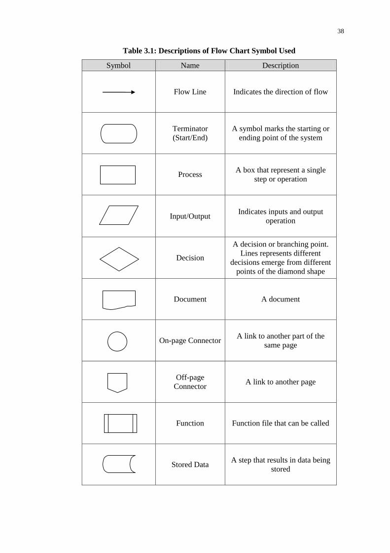
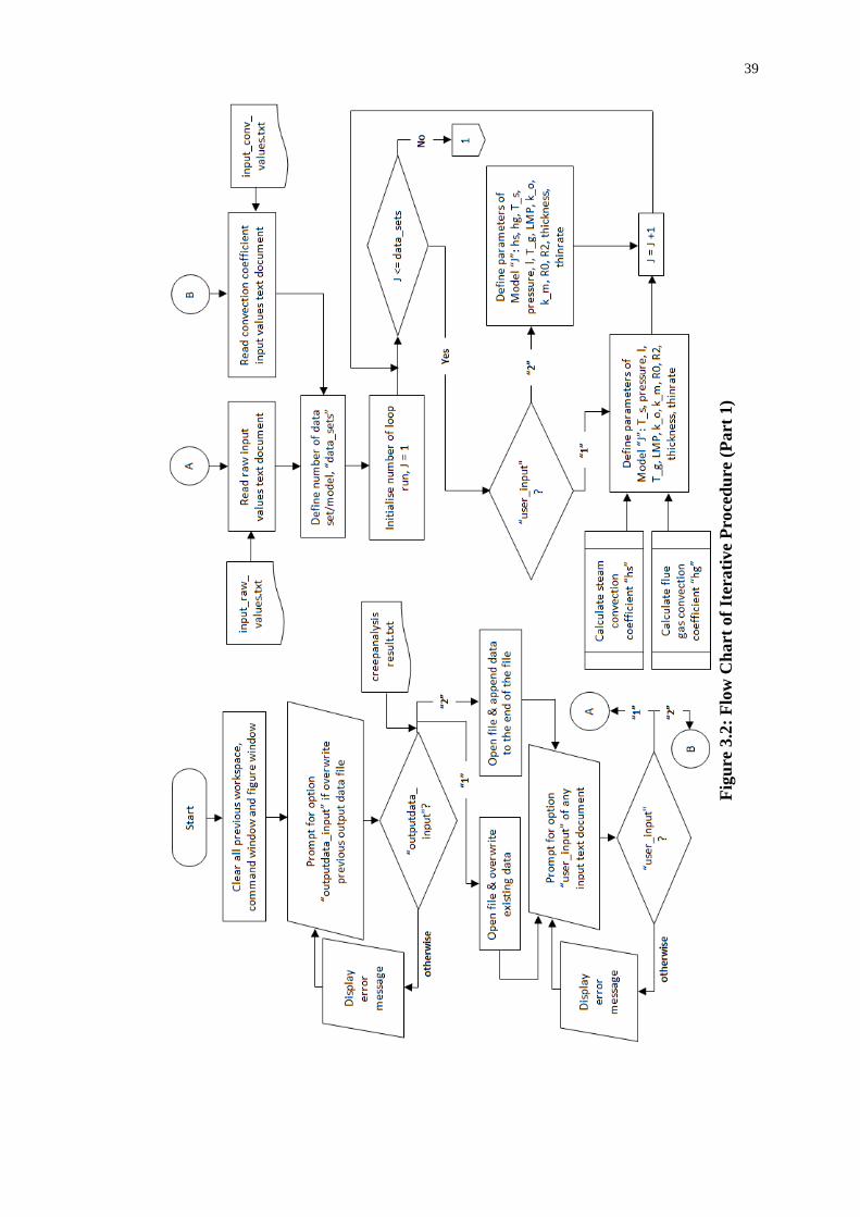
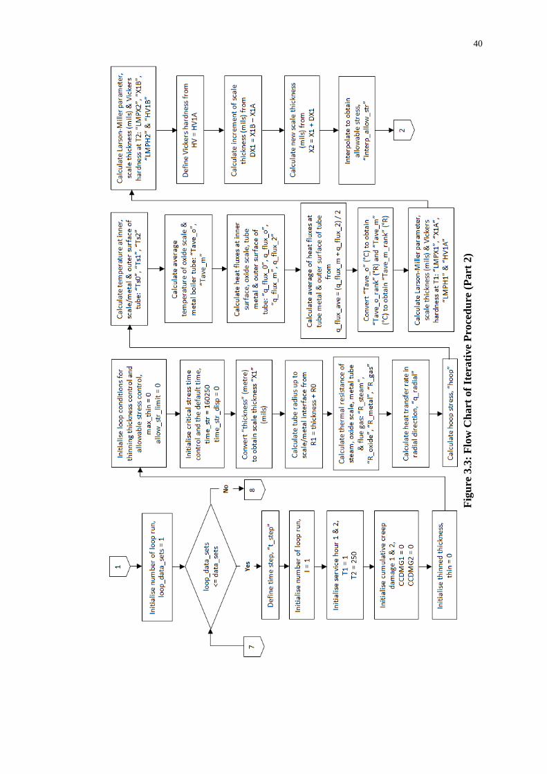
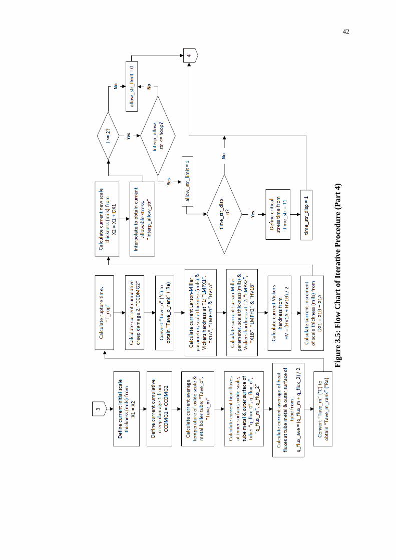
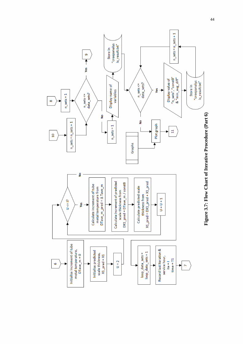
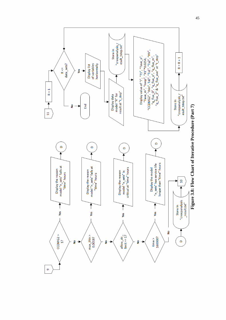
The flow charts of the proposed iterative procedure in MATLAB are
illustrated in Figure 3.2 to Figure 3.8 and the descriptions of symbols used are shown
in Table 3.1. Figure 3.1 illustrates the usage of both Off-page and On-page
connectors in joining different flow charts.
The flow chart starts from Figure 3.2 and proceeds to Figure 3.3 through the
Off-page Connector 1 on the right. The program continues until it reaches the Off-
page Connector 2 that links to Figure 3.4. If the program in Figure 3.4 fulfils the
conditions stated at the bottom left corner, it will proceed to Figure 3.5 through Off-
page Connector 3 and return back to Figure 3.4 through Off-page Connector 4,
otherwise follows the Off-page connector 5 to Figure 3.6 and continues to Figure 3.7
via Off-page Connector 6.
Based on Figure 3.7, the flow chart depicted on the left side brings the
program back to Figure 3.3 via Off-page Connector 7 and repeats the steps as
described in the previous paragraph, provided that the condition stated on the left
Page 54
37
side of Figure 3.3 is fulfilled. When the condition is no longer satisfied, the Off-page
Connector 8 connects the flow chart from Figure 3.3 to the flow chart on the right
side of Figure 3.7. An Off-page Connector 9 joins the program to the left flow chart
in Figure 3.8 when the condition specified on the top right corner is fulfilled and
returns it back to Figure 3.7 via Off-page Connector 10 at the bottom, otherwise the
flow chart follows the flow downward until it reaches Off-page Connector 11 that
connects to the flow chart on the right side of Figure 3.8. Eventually, the program
will end at the terminator symbol located at the middle part of the flow chart (right
side) in Figure 3.8.
Figure 3.1: An Illustration of Usage of Off-page and On-page Connectors
Page 55
38
Table 3.1: Descriptions of Flow Chart Symbol Used
Symbol Name Description
Flow Line Indicates the direction of flow
Terminator
(Start/End)
A symbol marks the starting or
ending point of the system
Process A box that represent a single
step or operation
Input/Output Indicates inputs and output
operation
Decision
A decision or branching point.
Lines represents different
decisions emerge from different
points of the diamond shape
Document A document
On-page Connector A link to another part of the
same page
Off-page
Connector A link to another page
Function Function file that can be called
Stored Data A step that results in data being
stored
Page 56
39
Fig
ure
3.2
: F
low
Ch
art
of
Iter
ati
ve
Pro
ced
ure
(P
art
1)
Page 57
40
Fig
ure
3.3
: F
low
Ch
art
of
Iter
ati
ve
Pro
ced
ure
(P
art
2)
Page 58
41
Fig
ure
3.4
: F
low
Ch
art
of
Iter
ati
ve
Pro
ced
ure
(P
art
3)
Page 59
42
Fig
ure
3.5
: F
low
Ch
art
of
Iter
ati
ve
Pro
ced
ure
(P
art
4)
Page 60
43
Fig
ure
3.6
: F
low
Ch
art
of
Iter
ati
ve
Pro
ced
ure
(P
art
5)
Page 61
44
Fig
ure
3.7
: F
low
Ch
art
of
Iter
ati
ve
Pro
ced
ure
(P
art
6)
Page 62
45
Fig
ure
3.8
: F
low
Ch
art
of
Iter
ati
ve
Pro
ced
ure
(P
art
7)
Page 63
46
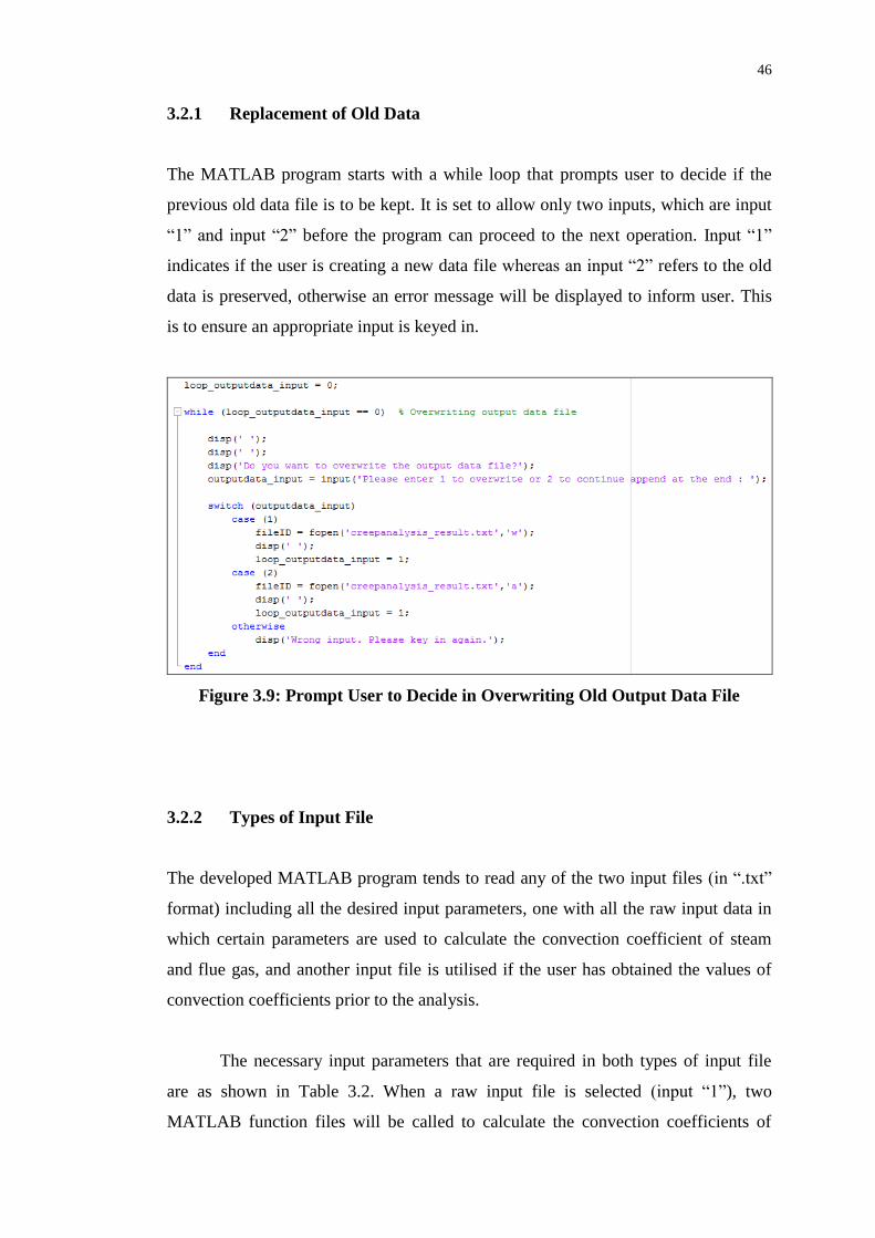
3.2.1 Replacement of Old Data
The MATLAB program starts with a while loop that prompts user to decide if the
previous old data file is to be kept. It is set to allow only two inputs, which are input
“1” and input “2” before the program can proceed to the next operation. Input “1”
indicates if the user is creating a new data file whereas an input “2” refers to the old
data is preserved, otherwise an error message will be displayed to inform user. This
is to ensure an appropriate input is keyed in.
Figure 3.9: Prompt User to Decide in Overwriting Old Output Data File
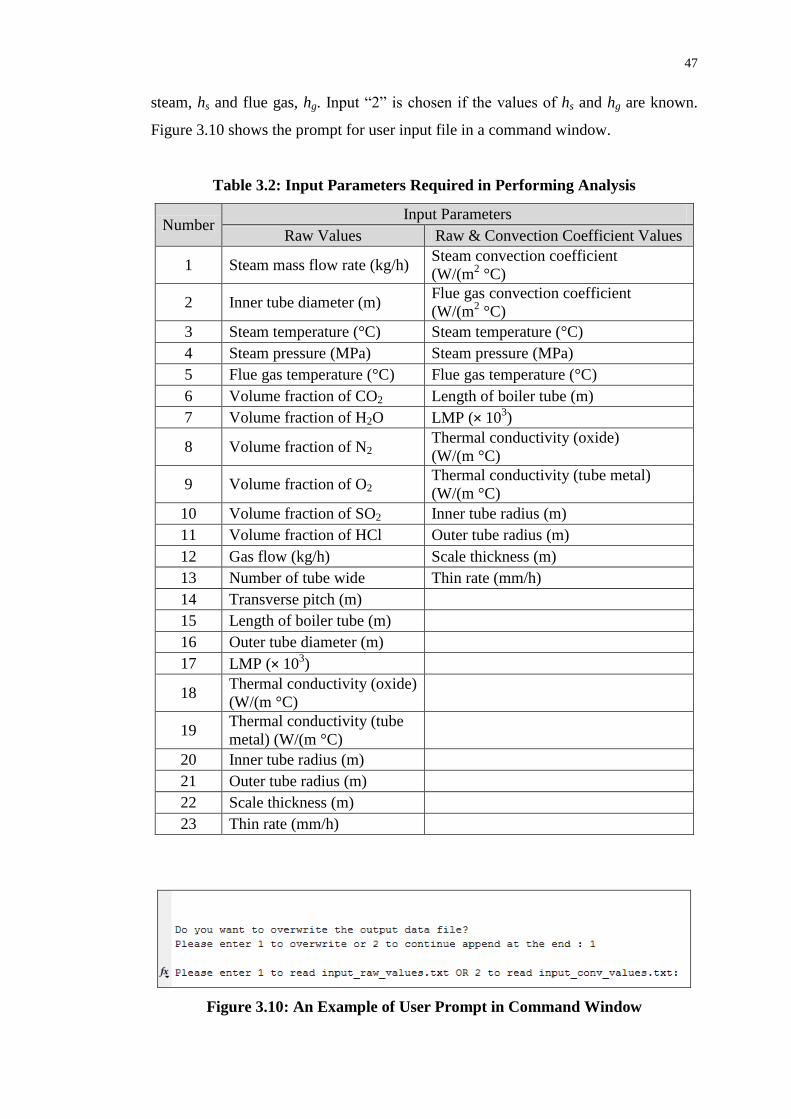
3.2.2 Types of Input File
The developed MATLAB program tends to read any of the two input files (in “.txt”
format) including all the desired input parameters, one with all the raw input data in
which certain parameters are used to calculate the convection coefficient of steam
and flue gas, and another input file is utilised if the user has obtained the values of
convection coefficients prior to the analysis.
The necessary input parameters that are required in both types of input file
are as shown in Table 3.2. When a raw input file is selected (input “1”), two
MATLAB function files will be called to calculate the convection coefficients of
Page 64
47
steam, hs and flue gas, hg. Input “2” is chosen if the values of hs and hg are known.
Figure 3.10 shows the prompt for user input file in a command window.
Table 3.2: Input Parameters Required in Performing Analysis
Number Input Parameters
Raw Values Raw & Convection Coefficient Values
1 Steam mass flow rate (kg/h) Steam convection coefficient
(W/(m2 °C)
2 Inner tube diameter (m) Flue gas convection coefficient
(W/(m2 °C)
3 Steam temperature (°C) Steam temperature (°C)
4 Steam pressure (MPa) Steam pressure (MPa)
5 Flue gas temperature (°C) Flue gas temperature (°C)
6 Volume fraction of CO2 Length of boiler tube (m)
7 Volume fraction of H2O LMP (× 103)
8 Volume fraction of N2 Thermal conductivity (oxide)
(W/(m °C)
9 Volume fraction of O2 Thermal conductivity (tube metal)
(W/(m °C)
10 Volume fraction of SO2 Inner tube radius (m)
11 Volume fraction of HCl Outer tube radius (m)
12 Gas flow (kg/h) Scale thickness (m)
13 Number of tube wide Thin rate (mm/h)
14 Transverse pitch (m)
15 Length of boiler tube (m)
16 Outer tube diameter (m)
17 LMP (× 103)
18 Thermal conductivity (oxide)
(W/(m °C)
19 Thermal conductivity (tube
metal) (W/(m °C)
20 Inner tube radius (m)
21 Outer tube radius (m)
22 Scale thickness (m)
23 Thin rate (mm/h)
Figure 3.10: An Example of User Prompt in Command Window
Page 65
48
3.2.3 Tube Life Prediction Conditional Control
There are few criteria which are most likely to cause rupture in boiler tube directly or
indirectly. A cumulative creep damage that reaches unity signifies the tube failure is
occurred. The reduction of thickness and stress accumulated in the tube wall
constitute to the critical state of the operating boiler tube. In the proposed analytical
iterative procedure, four stopping criteria are being used in controlling the loop. The
loop or iteration is forced to stop if any of the condition is unsatisfied, which
pinpoints the boiler tube is either in critical condition or has high risk in resulting
failure.
One of the conditions is the cumulative creep damage (CCDMG), which is
used to analyse the creep life of the boiler tube and indicates the possible service life
the tube has. The value of CCDMG must be equal or less than unity or one. For a
boiler tube that is in safe condition over a long period of time, the service life is
anticipated to operate longer than the optimum service hours of 160 000 h. Thus, the
maximum iteration is performed until service hours of 160 000 h.
The previous two conditions are treated as minimum requirements to be
fulfilled to ensure the boiler tube is safe to use. Another important factor to be
observed is the wall thinning effect of the tube. Thinning effect is more likely to
hasten the rupture of tube and reduce its service life provided that the operating
pressure is high. On the other hand, a boiler tube is not recommended to operate at
operational pressure that is too high as the hoop stress as a function of steam pressure
tends to exceed the maximum allowable stress of the tube. In this situation, the boiler
tube is said to be in critical state. On top of that, the tube will rupture if the stress
reaches its yield strength. A value of “0” refers to the hoop stress is still below the
maximum allowable stress while a value of “1” signal a warning of the critical state
experienced by the tube.
User has the options to turn off any of the last two conditions by placing a
symbol of “%” in front of the condition to convert the command code into a
comment tag. It is informed that the first two conditions should not be turning off as
they act as the fundamental requirements for the iterative procedure to perform. An
Page 66
49
illustration of the while loops with three and four conditional controls are shown in
Figure 3.11. Figure 3.12 shows an example of the analysis’ summary indicating the
root cause of the exiting loop.
Figure 3.11: Illustration of Four Conditional Controls (Top) and Three
Conditional Controls (Bottom)
Figure 3.12: An Example of Summary of the Analysis
3.2.4 Results Display and Graph Plotting
There are two types of displayed results from the MATLAB program, one that
including all the variable values in each iteration (increment of 250 h) as depicted in
Figure 3.13 while the other type displays extracted data at predetermined time step as
shown in Figure 3.14. The results also show if a particular model with or without the
wall thinning effect.
Furthermore, the developed MATLAB program has the ability to plot various
graphs by recalling separate function files as shown in Figure 3.15. The circled parts
show the file names of the graph. Similarly, the function file recalling can be turned
off by placing a “%” symbol in front of the command to convert it into a comment
tag. The MATLAB program limits maximum of six models for better visibility and
clarity of the plotted graph.
Page 67
50
Figure 3.13: Part of the Results Displayed (Complete Iterations)
Figure 3.14: Part of the Results Displayed At Predetermined Time Steps
Page 68
51
Figure 3.15: Separate Function Files for Graph Plotting
3.3 Correlation Function between Tube Metal Temperature Rise and Scale
Growth
The temperature increase in the tube metal wall and steam-side scale growth on the
inner tube wall are closely related. In the past, the common root cause that lead to the
failed superheater or reheater tubes were reported to be overheating of the tube over
long period of time. The formation of the scale on the inner wall of the tube can
inhibit the heat transfer and result in accumulation of temperature in the tube metal.
It was found that the linear relationship between the scale growth of
superheater and reheater tubes and the tube metal temperature increase could be
correlated with a constant B. This allows a study of the various operating conditions
of the boiler tube with respect to the correlation function. The increment of tube
metal temperature ΔTave,m as a function of increment of scale thickness ΔX over long
service hours can be expressed as:
Page 69
52
XBT (3.1)
where
ΔT = increment of tube metal temperature, °C
ΔX = increment of scale thickness, mils
B = constant correlating the temperature increase and scale growth
The increasing scale thickness is the scale thickness in mils. One mil is
equivalent to one thousandth (1 × 10⁻³
) of an inch or 0.0254 mm. From the Equation
3.1, it could be deduced that a constant B acts as a multiplier to every increment of
scale thickness corresponding to each increment of tube metal temperature. When the
constant B is greater than one, it describes that the increment is more significant in
temperature or relatively less in scale thickness and vice versa.
In order to embark on the development of a constant, a set of data for the
scale thickness or temperature of the tube metal over the service hours is necessary.
In this project, the data of scale thickness was used in the prediction of temperature
increase in the tube. By using the iterative procedure proposed in this chapter, the
values for scale thickness for all the iterations up to a maximum time step of 160 000
h were stored. The increment of scale thickness ΔX at every time step was
determined.
After the data collection of the incremental thickness of scale, a constant B
was estimated by undergoing trial and error process and selected a value which
produced the lowest percentage of difference from the estimated incremental tube
metal temperature. The first increment of tube metal temperature estimated by the
constant B was added to the average tube metal temperature at the first iteration (I =
1) to form new temperature. The second temperature rise was added to this new
temperature to estimate the temperature at second iteration (I = 2). This step was
repeated for the rest of iterations. An inverse way can be done to estimate the scale
thickness by using the tube metal temperature increase obtained from the iterative
procedure instead of scale thickness. It was proposed that the trial and error process
arises with an initial of 0.01 until a constant of 5. The range of the tested constant
Page 70
53
value can be decided by the user. A total of 500 possible constant B values can be
used.
3.4 Models Preparation of Analysis
Table 3.3 shows three different geometries of superheater and reheater tubes used in
the analysis. These three tubes were evaluated. The correlation function of the seven
models with different operating conditions and heat transfer parameters used in this
study are shown in Table 3.4. Model 1 was set as the default model in each analysis.
Apart from that, other relevant parameters that required in the analytical iterative
method are tabulated in Tables 3.5 to 3.7. The assumptions made in the analysis are
stated as below:
1. The heat transfer is in steady state and one-dimensional.
2. The thermal conductivity of oxide layer and tube metal remained constant for
the whole analysis
3. The convection coefficients of steam and flue gas are uniform over the inner
surface and outer surface of the boiler tubes respectively.
4. Oxide scale growth rate and wall thinning rate of the boiler tubes are uniform.
5. The steam temperature and flue gas temperature are kept constant throughout
the entire process.
6. The thermal properties of the boiler tube have no changes during the
operations.
Table 3.3: Geometries of Tube
Tube Inner Radius (m) Outer Radius (m) Wall Thickness (m)
1 0.0219 0.0254 0.0035
2 0.0219 0.0264 0.0045
3 0.0219 0.0274 0.0055
Page 71
54
Table 3.4: Models for Failure Analysis of Tube
Model Tube
Steam
Temperature
(°C )
Steam Mass
Flow Rate
(kg/h)
Flue Gas
Temperature
(°C )
Operating
Internal Pressure
(MPa)
1 1 540 3600 800 4
2 1 540 3800 800 4
3 1 540 4000 800 4
4 1 560 3600 800 4
5 1 580 3600 800 4
6 1 540 3600 900 4
7 1 540 3600 1000 4
8 2 540 3600 800 4
9 3 540 3600 800 4
Table 3.5: Solid Material Properties for Boiler Tube
Water Wall Properties
Tube Material SA213-T22
Thermal Conductivity, km (W/m °C) 34.606
Fe3O4 Iron Oxide (Magnetite)
Thermal Conductivity, ko (W/m °C) 0.592
Table 3.6: Parameters Required in Determining Gas Mass Velocity, G
Gas Flow (kg/h) 400 000
Number of Tube Wide 32
Transverse Pitch (m) 0.1016
Tube Length (m) 10
Table 3.7: Compositions of Flue Gas at 15 % Air
Nitrogen (mole %) 71.08
Oxygen (mole %) 2.46
Carbon Dioxide (mole %) 8.29
Water (mole %) 18.17
Page 72
CHAPTER 4
4 RESULTS AND DISCUSSION
4.1 Validation of the Developed MATLAB Program
The accuracy of the scale thickness and cumulative creep damage obtained by the
proposed iterative technique using developed MATLAB program is crucial to the
prediction of the remaining life of superheater and reheater tubes. In the literature,
Purbolaksono et al. (2009b) have reported the details of reheater tube failed in Kapar
Power Station Malaysia. Those details such as service life, scale thickness and other
heat transfer parameters were adopted in this project for results validation purposes.
The reheater tube failed at Kapar Power Station Malaysia has been analysed
and examined by Purbolaksono et al. (2009b). The tube was situated at a distance
from the burner and operated under average steam pressure of 4 MPa. The operating
steam temperature and flue gas temperature for the tubes were 576 °C and 800 °C
respectively. The details of the reheater tube are tabulated in Table 4.1 to 4.3.
Few parameters including gas flow Wg, number of tube wide Nw, transverse
pitch St and tube length L that are needed to calculate the gas mass velocity G are
shown in Table 4.2. The estimated steam convection coefficient hs at internal tube
surface and the flue gas convection coefficient hg at external tube surface are
tabulated in Table 4.3.
Page 73
56
Table 4.1: Geometry, Service Time and Inner Scale Thickness of the Tubes and
the Year of Failure
Inner
Radius (m)
Tube Thickness
(mm)
Service Time
(h)
Scale Thickness
(mm)
Year of
Failure
0.0219 3.5 117 522 0.58 2003
(Purbolaksono et al., 2009b. p.906)
Table 4.2: Parameters Required in Determining Gas Mass Velocity G
Gas Flow (kg/h) 500 000
Number of Tube Wide 50
Transverse Pitch (m) 0.1016
Tube Length (m) 8
(Purbolaksono et al., 2009b. p.906)
Table 4.3: The Estimated Steam and Flue Gas Convection Coefficients
hs (W/m2 °C) hg (W/m
2 °C)
2053.65 126.01
(Purbolaksono et al., 2009b. p.907)
The Larson-Miller parameter (LMP) can be determined by the Equations 2.18
– 2.20 and the LMP chart shown in Figure 2.11. Purbolaksono et al. (2009b) have
estimated the LMP value to be 39 900. With the aid of LMP value, cumulative creep
damage can be obtained as a measure of damage for boiler tube. The cumulative
creep damage denotes the life expectancy of tube. Once the cumulative creep damage
is equal or greater than unity (one), the tube is said to be failed and ruptured.
In this project, the proposed iterative technique using MATLAB program was
capable to generate similar results with the Finite Element Method (FEM) reported
by Purbolaksono et al. (2009b). By using the same operational heat transfer
parameters, the estimated remaining life of reheater tube in terms of cumulative
creep damage and other parameters such as scale thickness, tube metal temperature
Page 74
57
and hardness were obtained. Table 4.4 shows the comparison of estimated scale
thickness and the cumulative creep damage while Table 4.5 shows the comparison of
estimated values for average tube metal temperature and Vickers hardness.
Table 4.4: Estimations of Scale Thickness and Cumulative Creep Damage by
MATLAB Program and Other Authors (FEM)
Service
Hour (h)
Scale Thickness (mm) Cumulative Creep Damage
MATLAB FEM*
Percentage
Difference
(%)
MATLAB FEM*
Percentage
Difference
(%)
1 0.0000 0.0000 0.00 0.0000 0.0000 0.00
250 0.0559 0.0556 0.49 0.0007 0.0007 3.77
500 0.0740 0.0736 0.50 0.0015 0.0015 0.37
1000 0.0972 0.0965 0.69 0.0031 0.0031 0.56
2500 0.1383 0.1371 0.89 0.0085 0.0086 1.59
5000 0.1801 0.1783 1.02 0.0185 0.0189 2.23
10 000 0.2344 0.2315 1.24 0.0415 0.0429 3.38
20 000 0.3052 0.3008 1.47 0.0962 0.1010 4.79
40 000 0.3986 0.3916 1.79 0.2326 0.2485 6.38
60 000 0.4669 0.4584 1.85 0.3994 0.4231 5.60
80 000 0.5229 0.5133 1.88 0.5934 0.6227 4.70
100 000 0.5715 0.5610 1.87 0.8130 0.8463 3.93
117 522 0.6097 0.5982 1.92 1.0257 1.0613 3.35
* The results were obtained from the work done by Purbolaksono et al. (2009b)
Page 75
58
Table 4.5: Estimations of Average Temperature of Tube Metal and Vickers
Hardness by MATLAB Program and Other Authors (FEM)
Service
Hour (h)
Average Temperature of Tube
Metal (°C) Vickers Hardness (HV)
MATLAB FEM*
Percentage
Difference
(%)
MATLAB FEM*
Percentage
Difference
(%)
1 592.11 591.88 0.04 317.75 317.92 0.05
250 594.70 594.46 0.04 233.53 233.72 0.08
500 595.52 594.98 0.09 225.12 223.56 0.70
1000 596.56 596.31 0.04 215.78 211.12 2.21
2500 598.39 598.11 0.05 202.21 198.24 2.00
5000 600.20 599.91 0.05 191.17 186.88 2.30
10 000 602.51 602.18 0.05 179.50 175.06 2.54
20 000 605.43 605.05 0.06 167.13 162.65 2.76
40 000 609.14 608.67 0.08 153.94 151.53 1.59
60 000 611.76 611.25 0.08 145.76 144.20 1.08
80 000 613.85 613.31 0.09 139.71 138.64 0.77
100 000 615.62 615.06 0.09 134.88 134.11 0.57
117 522 616.99 616.49 0.08 131.28 131.61 0.25
* The results were obtained from the work done by Purbolaksono et al. (2009b)
According to the Table 4.4, the estimated scale thickness using MATLAB
program was found to have less than 2 % of differences from the results estimated by
Finite Element Method. However, the results from the MATLAB and FEM have the
differences of less than 6.5 % and were fairly consistent throughout the reheater tube
operation. Apart from that, the values of average tube metal temperature and Vickers
hardness were very similar between the two prediction methods. In overall, the
estimated results using MATLAB program have insignificant differences compared
to the works done by Purbolaksono et al. (2009b) using FEM. Therefore, it shows
that the prediction method of MATLAB program is in good conformity with the
FEM results. Figure 4.1 to 4.4 depict the comparison between the estimated results
and the actual data.
Page 76
59
Figure 4.1: Comparison between the MATLAB and FEM Results In Terms of
Cumulative Creep Damage
Figure 4.2: Comparison of MATLAB, FEM and Actual Data In Terms of Scale
Thickness
Page 77
60
Figure 4.3: Comparison between the MATLAB and FEM Results In Terms of
Tube Metal Temperature
Figure 4.4: Comparison between the MATLAB and FEM Results In Terms of
Vickers Hardness
Page 78
61
Figure 4.1 depicts the comparison of the predicted cumulative creep damage
between the MATLAB program and the FEM. The comparisons of the MATLAB
and FEM results with the actual data (Kapar Power Station Malaysia) are presented
in Table 4.6 and 4.7. According to the Table 4.6, the cumulative creep damage of
actual data is considered as unity (one) in which reheater tube failure has occurred.
At the service hours of 117 522 h, it was found that the predicted cumulative creep
damage obtained from MATLAB and FEM have only small variations as compared
to the actual situation. Table 4.7 shows that the MATLAB result has a difference of
2.57 % from the actual data whereas the FEM result has 6.13 % of difference. It
could be seen that the life expectancy by MATLAB program is closer to the actual
failure service hours reported by Kapar Power Station Malaysia than the prediction
by other authors. This has proved that the utilisation of developed MATLAB
program in predicting the remnant life of the boiler tubes is reliable.
Table 4.6: Cumulative Creep Damage at Failure Service Hours
Type of Result Cumulative Creep
Damage
Failure Service
Hour (h)
MATLAB 1.0257
117 522 FEM 1.0613
Actual Data 1
Table 4.7: Percentage Differences between Estimated Results and Actual Data
(Life Expectancy)
Percentage of Difference (%)
MATLAB FEM
Service Life of
Actual Data 2.57 6.13
The results obtained from the MATLAB program were also compared with
the FEM results and actual data in terms of scale thickness as shown in Table 4.8.
From Table 4.8, thicker oxide scale layer was found on the inner surface of the
reheater tube than the scale thickness reported at Kapar Power Station Malaysia.
Based on Table 4.9, the Finite Element Method proposed by Purbolaksono et al.
Page 79
62
(2009b) has closer scale thickness prediction, which is 3.14 % difference from the
measured scale thickness. The percentage difference of the results from MATLAB
program is also small despite greater variation than FEM. The difference of 5.12 %
or 0.0297 mm in terms of scale thickness is acceptable.
Table 4.8: Scale Thickness at Failure Service Hours
Type of Result Scale Thickness
(mm)
Failure Service
Hour (h)
MATLAB 0.6097
117 522 FEM 0.5982
Actual Data 0.58
Table 4.9: Percentage Differences between Estimate Results and Actual Data
(Scale Thickness)
Percentage of Difference (%)
MATLAB FEM
Scale Thickness
of Actual Data 5.12 3.14
The percentage differences with less than 7 % in both predictions of remnant
life and scale thickness of the reheater tube implies that the results from MATLAB
program is capable in signalling warning signs before the failure tends to occur. The
proposed iterative method using MATLAB program may be used to assist predictive
maintenance of boiler tube in power plant. However, it is recommended to set up a
range of the service time for a conservative prediction of the remnant life and scale
thickness of boiler tube. By evaluating the obtained results, a suggestion of ± 10 %
from the predicted service hours and scale thickness is sufficient. The workers or
maintenance teams should carry out maintenance activities including inspections and
condition monitoring more regularly especially within the range of failure service
hour. During that period, awareness and cautious observation are very important in
order to identify the presence of defect prior to failure.
Page 80
63
4.2 Evaluation of Constant B in Correlation Function
A constant value that correlates the oxide scale formation on the inner surface of
boiler tube wall and the increasing temperature in the tube metal is affected by
different operating heat transfer parameters. The effects by these parameters are
discussed in the following sub-subsections. The average percentage difference of
predicted tube metal temperature from each model is calculated for accuracy
checking.
4.2.1 Tube Geometry
The models with different outer tube radii as shown in Table 4.10 were assessed with
the generated constant B. The Model 1 has the smallest outer tube radius with the
thinnest thickness, following by Model 8 and Model 9. The constant B for each
model with their respective accuracy is tabulated in Table 4.11.
Table 4.10: Models Used for Tube Geometry Analysis
Model 1
(Tube 1)
Model 8
(Tube 2)
Model 9
(Tube 3)
Inner Radius (m) 0.0219 0.0219 0.0219
Outer Radius (m) 0.0254 0.0264 0.0274
Steam Temperature, Ts (°C) 540 540 540
Flue Gas Temperature, Tg (°C) 800 800 800
Calculated Convection Coefficient, hs
(W/m2 °C)
2344.27 2344.27 2344.27
Calculated Convection Coefficient, hg
(W/m2 °C)
121.85 122.91 124.17
Steam Mass Flow Rate, ṁs (kg/h) 3600 3600 3600
Page 81
64
Table 4.11: Generated Constant B and Average Percentage of Difference In
Terms of Tube Metal Temperature (Model 1, 8, 9)
Model Constant B Average Percentage
of Difference (%)
1 1.29 0.0162
8 1.34 0.0175
9 1.38 0.0193
According to Figure 4.5, it could be seen that the thicker tubes (greater outer
radius) result in higher tube metal temperature. The gradient of the curve is
significantly steeper for Model 9 than the rest. At the same time, the oxide scale
growth is also greater in thicker tubes (greater outer radius) as shown in Figure 4.6,
even though the difference is not significant.
The increasing constant B describes the phenomenon in which the increment
of the temperature in tube wall as a function of time and scale thickness is relatively
greater than the increment of scale thickness and vice versa. This may be explained
as the oxide scale formation as a result of material deterioration from the changes of
material microstructure form a thermal barrier, which eventually leads to higher
temperature accumulated in the thicker tube wall. The higher constant B denotes
greater impact to the increment of tube metal temperature than the oxide scale
growth. In fact, the superheater and reheater tube geometry has a direct effect to the
steam-side oxide scale growth and the temperature increase in the tube.
Page 82
65
Figure 4.5: Estimated Tube Metal Temperature with Different Outer Radius
(Tube) by Constant Estimation
Figure 4.6: Estimated Scale Thickness with Different Outer Radius (Tube)
Page 83
66
4.2.2 Steam Mass Flow Rate
The steam mass flow rate is essential in the heat transfer from the tube wall to the
steam region inside the tube. Model 1, Model 2 and Model 3 were employed in this
analysis as shown in Table 4.12. Higher steam mass flow rate contributes to higher
convection coefficient of steam and reduces the temperature increased in tube metal.
An insignificant increase in value of constant B describes that the incremental tube
wall temperature drops at the similar rate, but slightly further than the scale thickness.
Table 4.12: Models Used for Mass Flow Rate Analysis
Model 1
(Tube 1)
Model 2
(Tube 1)
Model 3
(Tube 1)
Inner Radius (m) 0.0219 0.0219 0.0219
Outer Radius (m) 0.0254 0.0254 0.0254
Steam Temperature, Ts (°C) 540 540 540
Flue Gas Temperature, Tg (°C) 800 800 800
Calculated Convection Coefficient, hs
(W/m2 °C)
2344.27 2447.89 2550.43
Calculated Convection Coefficient, hg
(W/m2 °C)
121.85 121.85 121.85
Steam Mass Flow Rate, ṁs (kg/h) 3600 3800 4000
Since the constant B generated as presented in Table 4.13 are greater than one,
the increasing of temperature is still higher than the increment of scale thickness by
comparing Figure 4.7 and Figure 4.8. Contrarily, poor mass flow rate of the steam
may cause tube wall to have higher temperature and thicker oxide scale layer, which
could to lead to the early tube rupture.
Table 4.13: Generated Constant B and Average Percentage of Difference In
Terms of Tube Metal Temperature (Model 1, 2, 3)
Model Constant B Average Percentage
of Difference (%)
1 1.29 0.0162
2 1.3 0.0154
3 1.31 0.0154
Page 84
67
Figure 4.7: Estimated Tube Metal Temperature with Different Steam Mass
Flow Rate by Constant Estimation
Figure 4.8: Estimated Scale Thickness with Different Steam Mass Flow Rate
Page 85
68
4.2.3 Steam Temperature
The heat transfers parameters of models used and generated constant B are shown in
Table 4.14 and Table 4.15. From Figure 4.9, the tube that operated at higher steam
temperature causes the tube metal temperature at the beginning of operation to be
higher. The decreasing value of estimated constant B can be seen when the design
temperature rises, which indicates that the increment of tube metal temperature with
higher operational temperature is lesser than the increment with lower operational
temperature. In other words, the increment of temperature in the tube is getting closer
(or smaller difference) to the increment of scale thickness. The increasing of the
gradient of curves with higher steam temperature and lower constant B in Figure 4.10
is more significant than the increasing of gradient in Figure 4.9. These phenomena
show that the transfer of heat from the flue gas across the tube, and to the steam is
considerably impaired by the smaller temperature difference across the tube. This
may result in more heat in the tube wall whereas the oxidation resistance at the inner
tube wall reduces and cause greater scale formation.
In addition, Model 5 was predicted to have shorter service life than Model 1
and Model 4, which tends to fail before 160000 service hours. It can be deduced that
the steam temperature is one of the factors that influence the life expectancy of boiler
tube significantly.
Table 4.14: Models Used for Steam Temperature Analysis
Model 1
(Tube 1)
Model 4
(Tube 1)
Model 5
(Tube 1)
Inner Radius (m) 0.0219 0.0219 0.0219
Outer Radius (m) 0.0254 0.0254 0.0254
Steam Temperature, Ts (°C) 540 560 580
Flue Gas Temperature, Tg (°C) 800 800 800
Calculated Convection Coefficient, hs
(W/m2 °C)
2344.27 2368.79 2392.66
Calculated Convection Coefficient, hg
(W/m2 °C)
121.85 121.85 121.85
Steam Mass Flow Rate, ṁs (kg/h) 3600 3600 3600
Page 86
69
Table 4.15: Generated Constant B and Average Percentage of Difference In
Terms of Tube Metal Temperature (Model 1, 4, 5)
Model Constant B Average Percentage
of Difference (%)
1 1.29 0.0162
4 1.16 0.0338
5 1.03 0.0549
Figure 4.9: Estimated Tube Metal Temperature with Different Steam
Temperature by Constant Estimation
Page 87
70
Figure 4.10: Estimated Scale Thickness with Different Steam Temperature
4.2.4 Flue Gas Temperature
The change of flue gas temperature will affect the convection coefficient of flue gas
as shown in Table 4.16. It can be deduced from Figure 4.11 and Figure 4.12 that the
combination of temperature and convection coefficient of flue gas has drastic effect
to the temperature increase and oxide scale growth.
Table 4.17 also shows a significant increase in constant B, which implies
higher flue gas temperature leads to a greater increment of both the tube metal
temperature and the scale thickness, whereby the increment value for temperature is
approximately 83 % more in Model 6 and 138 % more in Model 7 than the
incremental scale thickness every 250 h. This may be explained as greater heat
transfer from the flue gas into the tube and increase the temperature in the tube metal
more swiftly than the growing of oxide layer. The vast changes in temperature are
critical as it may lead to potential failure of the tube.
Page 88
71
Table 4.16: Models Used for Flue Gas Temperature Analysis
Model 1
(Tube 1)
Model 6
(Tube 1)
Model 7
(Tube 1)
Inner Radius (m) 0.0219 0.0219 0.0219
Outer Radius (m) 0.0254 0.0254 0.0254
Steam Temperature, Ts (°C) 540 540 540
Flue Gas Temperature, Tg (°C) 800 900 1000
Calculated Convection Coefficient, hs
(W/m2 °C)
2344.27 2344.27 2344.27
Calculated Convection Coefficient, hg
(W/m2 °C)
121.85 127.19 132.41
Steam Mass Flow Rate, ṁs (kg/h) 3600 3600 3600
Table 4.17: Generated Constant B and Average Percentage of Difference In
Terms of Tube Metal Temperature (Model 1, 6, 7)
Model Constant B Average Percentage
of Difference (%)
1 1.29 0.0162
6 1.83 0.0343
7 2.38 0.0719
Page 89
72
Figure 4.11: Estimated Tube Metal Temperature with Different Flue Gas
Temperature by Constant Estimation
Figure 4.12: Estimated Scale Thickness with Different Flue Gas Temperature
Page 90
73
4.2.5 Summary
A constant value B that is greater than one indicates the incremental tube metal
temperature is more than the incremental scale thickness, while a constant value that
is smaller than one indicates the other way round. The incremental value will be the
same for both the tube metal temperature and scale thickness if the constant B is
exactly one. From the four analyses discussed earlier, all the estimated B constants
were found to be greater than one. By increasing the tube geometry, steam mass flow
rate and flue gas temperature, the constant B was found to be increased accordingly,
which signified more impact to the increment of tube metal temperature. However,
the constant B decreased with the rose of steam temperature. It denoted less effect of
the change of particular parameter to the tube metal temperature.
It was found that all the estimated tube metal temperatures by using the
generated constant B have less than 0.1 % difference compared to the temperature
predicted by iterative procedure. Therefore, the estimation using constant B is
reliable and has very similar temperature curve with the result from MATLAB
program.
Page 91
CHAPTER 5
5 CONCLUSIONS AND RECOMMENDATIONS
5.1 Conclusions
An iterative analytical procedure used for boiler tube analysis has been proposed and
implemented in MATLAB. This technique was proved to be a reliable tool in
estimating the service life of boiler tubes associated with various temperature
dependent parameters such as oxide scale growth, wall thinning, hoop stress, heat
flux, hardness, and creep damage of the tubes.
The implementation of the iterative analytical procedure coupled with the
comparisons with data of failed boiler tubes reported at Kapar Power Station
Malaysia and the results from other authors were presented. The estimated service
life of tube in terms of cumulative creep damage was found to have less than 3 % of
difference with the actual data. In order to implement the proposed iterative method
with conservative estimations, a suggested time range of the service hours is ± 10 %
of the estimated service life. The accuracy of the iterative analytical procedure in life
prediction of tube was satisfied. The prediction of scale thickness was accurate, with
a difference of less than 6.5 % and has better estimation than other authors. In
general, the results obtained from the MATLAB program were shown to be in good
conformity with the actual data and work from other authors.
Page 92
75
The tube metal temperature is one of the crucial factors in affecting the scale
growth on the inner surface of the tube. The formation of oxide layer was found to be
the root cause of many tube failure cases by mechanical and corrosion. A proposed
constant estimation technique with appropriate methodology aids the prediction of
increased temperature in tube metal and scale thickness in line with the failure
analysis of the tube. A constant B correlating the tube metal temperature increase and
scale thickness growth was found to be useful in estimating the significant effect in
either the incremental temperature or incremental scale thickness at an operation
condition.
Based on the study, the value of constant B may signal a warning of the
possible excessive tube metal temperature increase or scale thickness increase prior
to occurrence of failure tube. A value of constant closed to one denoted the
increasing rates of both the temperature and scale thickness are similar. When the
constant B was greater than one, the temperature of tube increased more than scale
thickness and vice versa if the constant B was smaller than one. An increase of
constant B was interpreted as more rises of tube temperature in relation to the scale
thickness, which could encourage greater formation of oxide scale and lead to early
tube rupture. On the other hand, a decreased constant B showed a more rapid growth
rate of oxide scale that tends to inhibit the heat transfer across the tube. A haste of
scale growth rate can weaken the tube wall.
Therefore, the iterative analytical procedure and the correlation function
between the tube metal temperature change and scale growth may be utilised in
assisting the predictive maintenance in power plant such as condition monitoring
system. These two proposed techniques are capable to provide an estimation of boiler
tube life and other useful information without incurring high cost and much time
consumption.
Page 93
76
5.2 Limitation of Developed MATLAB Program
The current development of MATLAB program is only capable to perform analysis
on the boiler tube using the material of Alloy Steel Seamless Tube SA213-T12 and
SA213-T22. The maximum allowable stresses used in MATLAB are referred to
these two materials. Raw data of maximum allowable stress is required if other tube
material is to be used to carry out an analysis. Those values of maximum allowable
stress can be obtained from ASME Table 1A Section II Part D.
The number of models to be analysed is limited to maximum of six models in
a single simulation. This limitation helps to improve the visibility and clarity of the
plotted graph. Apart from that, certain graphs from the separated function files can
only plot one model at once due to the different types of comparison. For instance, a
graph of heat flux distribution contains four curves that representing four regions of
the tube wall (inner surface, scale layer, tube metal, and outer surface). It is not
recommended to compare with other models to avoid unnecessary confusion.
5.3 Recommendations
The boiler tube analysis can be improved by incorporating the proposed iterative
analytical procedure with other commercial software such as ANSYS. The iterative
analytical method is a numerical estimation using a regular time step and can only
perform analysis for one dimensional geometry. ANSYS is capable to demonstrate
and simulate the temperature distribution of complicated geometry that involves two
or more dimensions such as finned tube. Thus, a programming language that can
export the results obtained from the ANSYS to the MATLAB for further numerical
analysis is recommended. The tube metal temperature increase estimated by ANSYS
can be used in conjunction with the constant estimation method in which only
required a set of data for scale thickness and tube metal temperature over period of
time.
Page 94
77
The scope of the research can be extended by considering the thermal strain
experienced in the tube. The development of thermal stress and thermal strain as a
function of temperature, pressure and time can also lead to boiler tube failure. The
thermal strain generated can be studied in relation to the thermal expansion and
temperature and pressure loading of the boiler tube.
Page 95
78
REFERENCES
Chandra, K., Kain, V. and Dey, G. K., 2011. Failure of 2.25Cr-1Mo steel superheater
tubes in a fluidized bed combustor due to fireside corrosion. Materials
Characterization, 62, pp. 62-69.
Chaudhuri, S., 2006. Some aspects of metallurgical assessment of boiler tubes –
Basic Principles and case studies. Materials Science and Engineering A, 432, pp.
90-99.
Fry, A., Adams, B., Davis, K., Swensen, D., Munson, S. and Cox, W., 2011. An
investigation into the likely impact of oxy-coal retrofit on fire-side corrosion
behavior in utility boilers. International Journal of Greenhouse Gas Control, 5S,
pp. S179-S185.
Ganapathy, V., 1994. Steam Plant Calculations Manual. 2nd
ed. New York: Marcel
Dekker, Inc.
Ganapathy, V., 2003. Industrial Boilers and Heat Recovery Steam Generators:
Design, Applications, and Calculations. New York: Marcel Dekker, Inc.
Grote, K. H. and Antonsson, E. K., 2009. Springer Handbook of Mechanical
Engineering, Vols. 10. [E-book] New York: Springer. Available at: Google Books
<book.google.com> [Accessed 28 July 2012].
Hernas, A., Imosa, M., Formanek, B. and Cizner, J., 2004. High-temperature
chlorine-sulfur corrosion of heat-resisting steels. Journal of Materials Processing
Technology, 157-158, pp. 348-353.
Incropera, F. P., Dewitt, D. P., Bergman, T. L. and Lavine, A. S., 2007.
Fundamentals of Heat and Mass Transfer. 6th
ed. New Jersey: John Wiley & Sons,
Inc.
Jones, D. R. H., 2004. Creep failures of overheated boiler, superheater and reformer
tubes. Engineering Failure Analysis, 11, pp. 873-893.
Page 96
79
Ju, Y., & Liu, L. S., 2011. A high-efficiency nondestructive method for remote
detection and quantitative evaluation of pipe wall thinning using microwaves.
NDT&E International, 44, pp. 106-110.
Lande, B. V., Sonde, V. M., Undirwade, S. K. and Andhare, A. M., 2011.
Experimental Investigation & Analysis to Reduce Boiler Tube Failure in Thermal
Power Plant. International Journal of Engineering Research and Technology, 4(2),
pp. 229-246.
Li, L., Duan, Y., Cao, Y., Chu, P., Carty, R. and Pan, W. P., 2007. Field corrosion
tests for a low chromium steel carried out at superheater area of a utility boiler
with three coals containing different chlorine contents. Fuel Processing
Technology, 88, pp. 387-392.
Lim, K. L., 2010. Boiler Tube Failure Analysis by Analytical Approach. Bachelor
Thesis, Universiti Tunku Abdul Rahman. Malaysia.
Phongphiphat, A., Ryu, C., Yang, Y. B., Finney, K. N., Leyland, A., Sharifi, V. N.
and Swithenbank, J., 2010. Investigation into high-temperature corrosion in a
large-scale municipal waste-to-energy plant. Corrosion Science, 52, pp. 3861-
3874.
Port, R. D. and Herro, H. M., 1991. The Nalco Guide to Boiler Failure Analysis:
Nalco Chemical Company. [E-book] New York: McGraw-Hill, Inc. Available at:
Google Books <book.google.com> [Accessed 28 July 2012].
Prieto, M. M., Suárez, I., Fernández, F. J., Sánchez, H. and Viescas, C., 2007.
Application of a thermal model to a power plant reheater with irregular tube
temperatures. Applied Thermal Engineering, 27, pp. 185-193.
Psyllaki, P. P., Pantazopoulos, G. and Lefakis, H., 2009. Metallurgical evaluation of
creep-failed superheater tubes. Engineering Failure Analysis, 16, pp. 1420-1432.
Purbolaksono, J., Khinani, A., Rashid, A. Z., Ali, A. A., Ahmad, J. and Nordin N. F.,
2009a. A new method for estimating heat flux in superheater and reheater tubes.
Nuclear Engineering and Design, 239, pp. 1879-1884.
Purbolaksono, J., Khinani, A., Ali, A. A., Rashid, A. Z. and Nordin, N. F., 2009b.
Iterative technique and finite element simulation for supplemental condition
monitoring of water-tube boiler. Simulation Modelling Practice and Theory, 17,
pp. 897-910.
Purbolaksono, J., Khinani, A., Rashid, A. Z., Ali, A. A. and Nordin, N. F., 2009c.
Prediction of oxide scale growth in superheater and reheater tubes. Corrosion
Science, 51, pp. 1022-1029.
Page 97
80
Purbolaksono, J., Ahmad, J., Khinani, A., Ali, A. A. and Rashid, A. Z., 2010. Failure
case studies of SA213-T22 steel tubes of boiler through computer simulations.
Journal of Loss Prevention in the Process Industries, 23, pp. 98-105.
Rahman, M. M., Purbolaksono, J. and Ahmad, J., 2010. Root cause failure analysis
of a division wall superheater tube of a coal-fired power station. Engineering
Failure Analysis, 17, pp. 1490-1494.
Salman, B. H., Hamzah, M. Z., Purbolaksono, J., Inayat-Hussain, J. I., Mohammed,
H. A. and Muhieldeen, M. W., 2011. Determination of correlation functions of the
oxide scale growth and the temperature increase. Engineering Failure Analysis,
18, pp. 2260-2271.
Sohail, M. A. and Mustafa, A. I., 2007. A study on damages in alloyed super heater
tubes of thermal power station. Indian Journal of Engineering & Materilas
Sciences, 14, pp. 19-23.
Syed, A. U., Simms, N. J. and Oakey, J. E., 2012. Fireside corrosion of superheaters:
Effects of air and oxy-firing of coal and biomass. Fuel, 101, pp. 62-73.
Vértesy, G., Tomáš, I., Uchimoto, T. and Takagi, T., 2012. Nondestructive
investigation of wall thinning in layered ferromagnetic material by magnetic
adaptive testing. NDT&E International, 47, pp. 51-55.
Vikrant K. S. N., Ramareddy, G. V., Pavan, A. H. V. and Kulvir Singh, 2013.
Estimation of residual life of boiler tubes using steamside oxide scale thickness.
International Journal of Pressure Vessels and Piping, 104, pp. 69-75.
Viswanathan, R., 1993. Damage Mechanisms and Life Assessment of High-
Temperature components. [E-book] Ohio: ASM International. Available at:
Google Books <book.google.com> [Accessed 28 July 2012].
Viswanathan, R., Gehl, S., Paterson, S. R. and Grunloh, H., 1994. Life assessment of
superheater/reheater tubes in fossil boilers. Journal of Pressure Vessel Technology,
116(1), pp. 1-16.
Xu, L. J., Khan, J. A. and Chen, Z. H., 2000. Thermal load deviation model for
superheater and reheater of a utility boiler. Applied Thermal Engineering, 20, pp.
545-558.
Page 98
81
APPENDICES
APPENDIX A: MATLAB Program Codes (Main Program)
% -------------------------------------------------------------------------
% Complete script for Creep Analysis
% Filename : creepanalysis.m
% Done by : Ang Wei Bing & Edwin Lim
% Date : 27 June 2012
% Mod. Date : 7 April 2013
% -------------------------------------------------------------------------
% List of variables to be key-ed in as input (input CONV sequence.txt):
% hs = Convection coefficient of steam [W/m^2-degC]
% hg = Convection coefficient of flue gas [W/m^2-degC]
% T_s = Steam temperature [degC]
% pressure = Steam pressure [MPa]
% T_g = Flue gas temperature [degC]
% l = Length of boiler tube [m]
% LMP = Larson-Miller parameter (w.r.t. hoop stress) [x 10^3]
% k_o = Thermal conductivity of oxide scale [W/m-degC]
% k_m = Thermal conductivity of metal boiler tube [W/m-degC]
% R0 = Inner radius of the tube (up to steam side wall) [m]
% R2 = Outer radius of the tube (up to gas side wall) [m]
% thickness = Scale thickness [m]
% thinrate = Thin rate [mm/h]
% List of variables to be key-ed in to calculate hs (input RAW sequence.txt)
% m_dot_s = Mass flow rate of steam [kg/h]
% di = Inner diameter of tube [m]
% List of variables to be key-ed in to calculate hg (input RAW sequence.txt)
% y_CO2 = Volume fraction of CO2 (%/100)
% y_H2O = Volume fraction of H2O (%/100)
% y_N2 = Volume fraction of N2 (%/100)
% y_O2 = Volume fraction of O2 (%/100)
% y_SO2 = Volume fraction of SO2 (%/100)
% y_HCl = Volume fraction of HCl (%/100)
% w_g = Gas flow [kg/h]
% n_w = Number of tube wide
% s_t = Transverse pitch [m]
% do = Outer diameter of tube [m]
% List of important variables in program:
% T1 = Service hour 1 [h]
% T2 = Service hour 2 [h]
% CCDMG1 = Cumulative creep damage 1
% CCDMG2 = Cumulative creep damage 2
% X1 = Initial scale thickness [mils] (1 mils = 0.0254 mm)
% X2 = New scale thickness [mils] (1 mils = 0.0254 mm)
% R1 = Oxide radius of the tube (up to scale/metal interface) [m]
% R_steam = Thermal resistance of steam [degC/W]
% R_oxide = Thermal resistance of oxide scale [degC/W]
% R_metal = Thermal resistance of metal boiler tube [degC/W]
Page 99
82
% R_gas = Thermal resistance of flue gas [degC/W]
% q_radial = Heat transfer rate in radial direction [W]
% hoop = Hoop stress [MPa]
% Ts0 = Temperature of inner surface of boiler tube [degC]
% Ts1 = Temperature of scale/metal interface [degC]
% Ts2 = Temperature of outer surface of boiler tube [degC]
% Tave_o = Average temperature of oxide scale [degC]
% Tave_m = Average temperature of metal boiler tube [degC]
% DTave_m = Increment of average temperature of metal boiler tube [degC]
% Tave_o_rank = Average temperature of oxide scale [degRankine]
% Tave_m_rank = Average temperature of metal boiler tube [degRankine]
% q_flux_0 = Heat flux at inner surface of boiler tube [W/m^2]
% q_flux_o = Heat flux at oxide scale of boiler tube [W/m^2]
% q_flux_m = Heat flux at tube metal of boiler tube [W/m^2]
% q_flux_2 = Heat flux at outer surface of boiler tube [W/m^2]
% q_flux_ave = Average of heat fluxes at tube metal and outer surface [W/m^2]
% LMPX1 = Larson-Miller parameter for service hour 1 (w.r.t. scale thickness)
% LMPX2 = Larson-Miller parameter for service hour 2 (w.r.t. scale thickness)
% X1A = Scale thickness for service hour 1 [mils] (1 mils = 0.0254 mm)
% X1B = Scale thickness for service hour 2 [mils] (1 mils = 0.0254 mm)
% DX1 = Increment of scale thickness [mils] (1 mils = 0.0254 mm)
% LMPH1 = Larson-Miller parameter for service hour 1 (w.r.t. Vickers hardness)
% LMPH2 = Larson-Miller parameter for service hour 2 (w.r.t. Vickers hardness)
% HV1A = Vickers hardness for service hour 1
% HV1B = Vickers hardness for service hour 2
% HV = Vickers hardness
% thin = Thinned thickness [m]
% T_rup = Rupture time [h]
% DTave_m_pred = Increment of predicted average tube metal temperature [degC]
% Tave_m_pred = Predicted average tube metal temperature [degC]
% DX1_pred = Increment of predicted scale thickness [mils] (1 mils = 0.0254 mm)
% X1_pred = Predicted scale thickness [mils] (1 mils = 0.0254 mm)
% p_diff = Percentage of difference for predicted result [%]
% avg_p_diff = Average percentage of difference [%]
% min_avg_diff = Minimum average percentage of difference obtained [%]
% constB = Selected constant B
% List of general variables in program for special purposes:
% I = Iteration
% data_sets = Number of data set/model
% inputvalue = List of input values from text document
% outputdata_input = Option for output file overwritten
% user_input = Option for text document (input) selection
% loop_outputdata_input = Loop of output output file overwritten
% loop_user_input = Loop of text document selection
% loop_data_sets = Loop of main program
% a = Number of input variables in text document
% b = Number of data set/model in text document
% J = Indication of column (set/model number) in "inputvalue"
% variable
% setnum = Indication of row (set/model number) in each variable
% col = Indication of column (varying values) in each variable
% t_step = Predetermined time step
% tstep_count = Count of time step
% Z = Iteration at predetermined time step (vector quantity)
% max_thin = Maximum allowable thinning [m]
% allow_str_limit = Allowable stress switch control w.r.t. hoop stress
% (0-above limit, 1-below limit)
% time_str = Time where hoop stress exceeds allowable stress
% time_str_disp = Stress time switch control (0-no record time, 1-record time)
% allow_str_Temp_C = Temperature set for allowable stress [degC]
% allow_str_MPa = Allowable stress w.r.t. tube metal temperature [MPa]
% interp_allow_str = Interpolated allowable stress [MPa]
% test = Number of loop to test constant B
% test_constB = Test constant B
% W = Iteration for test constant
% W_switch = Test constant switch control [0-no record 'V' , 1-record
'V']
% V = Iteration at selected test constant B
% U = Iteration for scale thickness prediction
% ite = Last iteration of each data set/model
% time = Last service hour of each data set/model
% n_sets = Loop of data set/model (for summary of results)
% R = Loop of data set/model w.r.t. predetermined time step
% S = Loop of time step
% zi = Iteration at predetermined time step (scalar quantity)
Page 100
83
clear % clear workspace
clc % clear command window
clf % clear figure window
loop_outputdata_input = 0;
while (loop_outputdata_input == 0) % Overwriting output data file
disp(' ');
disp(' ');
disp('Do you want to overwrite the output data file?');
outputdata_input = input('Please enter 1 to overwrite or 2 to continue append at
the end : ');
switch (outputdata_input)
case (1)
fileID = fopen('creepanalysis_result.txt','w');
disp(' ');
loop_outputdata_input = 1;
case (2)
fileID = fopen('creepanalysis_result.txt','a');
disp(' ');
loop_outputdata_input = 1;
otherwise
disp('Wrong input. Please key in again.');
end
end
loop_user_input = 0;
while (loop_user_input == 0) % text document (input file) selection
user_input = input('Please enter 1 to read input_raw_values.txt OR 2 to read
input_conv_values.txt: ');
switch (user_input)
case (1)
fileID1 = fopen('input_raw_values.txt');
inputvalue = fscanf(fileID1, '%g %g %g %g %g %g', [23 6]);
fclose(fileID1);
[a,b] = size(inputvalue);
data_sets = b;
loop_user_input = loop_user_input + 1;
case (2)
fileID1 = fopen('input_conv_values.txt');
inputvalue = fscanf(fileID1, '%g %g %g %g %g %g', [13 6]);
fclose(fileID1);
[a,b] = size(inputvalue);
data_sets = b;
loop_user_input = loop_user_input + 1;
otherwise
disp('Wrong input. Please key in again.');
end
end
J = 1;
col = 1; % for all input variables in scalar quantity
while (J <= data_sets) % import input values from text document
setnum = J;
switch (user_input)
case (1)
[hs] = calc_hs(inputvalue,data_sets);
[hg] = calc_hg(inputvalue,data_sets);
T_s(setnum,col) = inputvalue(3,J);
pressure(setnum,col) = inputvalue(4,J);
l(setnum,col) = inputvalue(15,J);
Page 101
84
T_g(setnum,col) = inputvalue(5,J);
LMP(setnum,col) = inputvalue(17,J);
k_o(setnum,col) = inputvalue(18,J);
k_m(setnum,col) = inputvalue(19,J);
R0(setnum,col) = inputvalue(20,J);
R2(setnum,col) = inputvalue(21,J);
thickness(setnum,col) = inputvalue(22,J);
thinrate(setnum,col) = inputvalue(23,J);
J = J + 1;
case (2)
hs(setnum,col) = inputvalue(1,J);
hg(setnum,col) = inputvalue(2,J);
T_s(setnum,col) = inputvalue(3,J);
pressure(setnum,col) = inputvalue(4,J);
T_g(setnum,col) = inputvalue(5,J);
l(setnum,col) = inputvalue(6,J);
LMP(setnum,col) = inputvalue(7,J);
k_o(setnum,col) = inputvalue(8,J);
k_m(setnum,col) = inputvalue(9,J);
R0(setnum,col) = inputvalue(10,J);
R2(setnum,col) = inputvalue(11,J);
thickness(setnum,col) = inputvalue(12,J);
thinrate(setnum,col) = inputvalue(13,J);
J = J + 1;
end
end
loop_data_sets = 1;
while (loop_data_sets <= data_sets) % start of main program
setnum = loop_data_sets;
t_step(1,:) = [1, 250, 500, 1000, 2500, 5000, 10000, 20000, 40000, 60000, ...
80000, 100000, 120000, 140000, 160000]; % predetermined time step
tstep_count = 1;
I = 1;
T1 = 1;
T2 = 250;
CCDMG1 = 0;
CCDMG2(setnum,1) = 0;
thin(setnum,1) = 0;
max_thin(setnum,1) = 0;
allow_str_limit(setnum,1) = 0;
time_str(setnum,1) = 160250;
time_str_disp = 0;
X1(setnum,1) = (thickness(setnum,col)/0.0000254); % conversion from metre
% to mils for thickness
R1 = thickness(setnum,col) + R0(setnum,col); % unit in metre
% Reference from Fundamentals of Heat and Mass Transfer (6th ed.); ...
% F. P. Incropera et al.
% Equation 3.9; Page 99
R_steam = 1/(2*hs(setnum,col)*pi*R0(setnum,col)*l(setnum,col));
% Equation 3.28; Page 117
R_oxide = (log(R1/R0(setnum,col)))/(2*pi*k_o(setnum,col)*l(setnum,col));
% Equation 3.28; Page 117
R_metal = (log(R2(setnum,col)/R1))/(2*pi*k_m(setnum,col)*l(setnum,col));
% Equation 3.9; Page 99
R_gas = 1/(hg(setnum,col)*2*pi*R2(setnum,col)*l(setnum,col));
% Equation 3.29; Page 118
q_radial = (T_g(setnum,col) - T_s(setnum,col))/(R_steam + R_oxide + ...
R_metal + R_gas);
% Equation 3 from M. M. Rahman et al. journal - Root cause failure analysis ...
% of a division wall superheater tube of a coal-fired power station
hoop(setnum,1) = pressure(setnum,col)*(R0(setnum,col) + (R2(setnum,col)- ...
R0(setnum,col))/2)/(R2(setnum,col)-R0(setnum,col));
Page 102
85
Ts2(setnum,1) = T_g(setnum,col) - (R_gas*q_radial);
Ts1(setnum,1) = Ts2(setnum,1) - (R_metal*q_radial);
Ts0(setnum,1) = Ts1(setnum,1) - (R_oxide*q_radial);
Tave_o(setnum,1) = Ts0(setnum,1); % or Tave_o = (Ts0 + Ts1)/2; where Ts0 = Ts1
Tave_m(setnum,1) = (Ts1(setnum,1) + Ts2(setnum,1))/2;
% Reference from Fundamentals of Heat and Mass Transfer (6th ed.); ...
% F. P. Incropera et al.
% Equation 3.8; Page 99
q_flux_0(setnum,1) = hs(setnum,col)*(Ts0(setnum,1) - T_s(setnum,col));
% Table 3.3; Page 126
q_flux_o(setnum,1) = k_o(setnum,col)*(Ts1(setnum,1) - Ts0(setnum,1))/ ...
(R1*log(R1/R0(setnum,col)));
% Table 3.3; Page 126
q_flux_m(setnum,1) = k_m(setnum,col)*(Ts2(setnum,1) - Ts1(setnum,1))/ ...
(R1*log(R2(setnum,col)/R1));
% Equation 3.8; Page 99
q_flux_2(setnum,1) = hg(setnum,col)*(T_g(setnum,col) - Ts2(setnum,1));
q_flux_ave(setnum,1) = (q_flux_m(setnum,1) + q_flux_2(setnum,1))/2;
Tave_o_rank = Tave_o(setnum,1)*1.8 + 32 + 460;
Tave_m_rank = Tave_m(setnum,1)*1.8 + 32 + 460;
% deg Fahrenheit = deg Celsius * 1.8 + 32
% deg Rankine = deg Fahrenheit + 460
T_rup(setnum,1) = 10^((LMP(setnum,col)*1000)/(Tave_m_rank*1.0)-20);
LMPX1 = Tave_o_rank*(20 + log10(T1*1));
X1A = (10^(0.00022*LMPX1-7.25));
LMPX2 = Tave_o_rank*(20 + log10(T2*1));
X1B = (10^(0.00022*LMPX2-7.25));
DX1(setnum,1) = X1B - X1A;
X2(setnum,1) = X1(setnum,1) + DX1(setnum,1); % X1A,X1B,DX1,X1,X2 are in unit ...
% 'mils' (1/1000 inches) or ...
% (0.0254 mm)
% Reference from Damage Mechanisms and Life Assessment of High-Temperature ...
% Components; R. Viswanathan
LMPH1 = Tave_m_rank*(20 + log10(T1*1));
HV1A = 961.713 - (0.020669*LMPH1); % Equation 5.27; Page 237
HV(setnum,1) = HV1A;
LMPH2 = Tave_m_rank*(20 + log10(T2*1));
HV1B = 961.713 - (0.020669*LMPH2); % Equation 5.27; Page 237
% For T22 material: (from ASME Table 1A Metric Section II Part D)
allow_str_Temp_C = [65, 100, 125, 150, 200, 250, 300, 325, 350, 375, 400, ...
425, 450, 475, 500, 525, 550, 575, 600, 625, 650];
allow_str_MPa = [118, 118, 116, 114, 114, 114, 114, 114, 114, 114, 114, ...
114, 114, 100, 80.9, 64, 47.7, 34.5, 23.5, 15.5, 9.39];
% For T12 material: (from ASME Table 1A Metric Section II Part D)
% allow_str_Temp_C = [65, 100, 125, 150, 200, 250, 300, 325, 350, 375, 400, ...
% 425, 450, 475, 500, 525, 550, 575, 600, 625, 650];
% allow_str_MPa = [117, 116, 114, 114, 114, 114, 113, 112, 110, 109, 107, ...
% 106, 103, 101, 88.3, 61.9, 40.3, 26.4, 17.3, 11.7, 7.4];
interp_allow_str(setnum,1) = interp1(allow_str_Temp_C,allow_str_MPa, ...
Tave_m(setnum,1));
% indication of data set with thinning or without thinning
switch (thinrate(setnum,col))
case (0)
fprintf(fileID,'CREEP ANALYSIS RESULT WITHOUT THINNING: (DATA
MODEL %d)\r\n\r\n',loop_data_sets);
otherwise
fprintf(fileID,'CREEP ANALYSIS RESULT WITH THINNING: (DATA
MODEL %d)\r\n\r\n',loop_data_sets);
end
fprintf(fileID,'%6s %12s %12s %12s %12s %12s %12s %12s %12s %12s %12s %12s %12s %12s
%12s %12s %12s\r\n','I','T1','Tave_o','Tave_m','hoop','X1*0.0254','CCDMG2','thin','Ts
0','Ts1','Ts2','HV','q_flux_0','q_flux_o','q_flux_m','q_flux_2','q_flux_ave');
Page 103
86
% conditions to be fulfilled to continue looping
while (CCDMG2(setnum,I)<=1 && T1<=160000 && max_thin(setnum,1)<=0.0018 ...
&& allow_str_limit(setnum,1)~=1)
result = [I T1 Tave_o(setnum,I) Tave_m(setnum,I) hoop(setnum,I) ...
X1(setnum,I)*0.0254 CCDMG2(setnum,I) thin(setnum,I) Ts0(setnum,I) ...
Ts1(setnum,I) Ts2(setnum,I) HV(setnum,I) q_flux_0(setnum,I) ...
q_flux_o(setnum,I) q_flux_m(setnum,I) q_flux_2(setnum,I) ...
q_flux_ave(setnum,I)];
fprintf(fileID,'\r\n%6d %12d %12.3f %12.3f %12.3f %12.4f %12.4f %12.5f %12.3f %12.3f
%12.3f %12.3f %12.3f %12.3f %12.3f %12.3f %12.3f\r\n',result);
% record the particular iteration when predetermined time step reached
while (T1 == t_step(tstep_count))
Z(setnum,tstep_count) = I;
if tstep_count <= (numel(t_step)-1)
tstep_count = tstep_count + 1;
else
tstep_count = 1; % reset the count before the time step exceeds ...
% 15th value
end
end
% thickness control (limit maximum thinning)
max_thin(setnum,1) = (thin(setnum,I)-thin(setnum,1)) + (R1-R0(setnum,col));
I = I + 1;
thickness(setnum,col) = X2(setnum,I-1)*0.0000254;
R1 = thickness(setnum,col) + R0(setnum,col);
thin(setnum,I) = (thinrate(setnum,col)*T1)/1000;
R_steam = 1/(2*hs(setnum,col)*pi*R0(setnum,col)*l(setnum,col));
R_oxide = (log(R1/R0(setnum,col)))/(2*pi*k_o(setnum,col)*l(setnum,col));
R_metal = (log((R2(setnum,col)-thin(setnum,I))/R1))/(2*pi*k_m(setnum,col) ...
*l(setnum,col));
R_gas = 1/(hg(setnum,col)*2*pi*(R2(setnum,col)-thin(setnum,I))*l(setnum,col));
q_radial = (T_g(setnum,col) - T_s(setnum,col))/(R_steam + R_oxide + ...
R_metal + R_gas);
hoop(setnum,I) = pressure(setnum,col)*(R0(setnum,col) + (R2(setnum,col)- ...
R0(setnum,col)-thin(setnum,I))/2)/(R2(setnum,col)-R0(setnum,col)- ...
thin(setnum,I));
Ts2(setnum,I) = T_g(setnum,col) - (R_gas*q_radial);
Ts1(setnum,I) = Ts2(setnum,I) - (R_metal*q_radial);
Ts0(setnum,I) = Ts1(setnum,I) - (R_oxide*q_radial);
T1 = T2;
T2 = T2 + 250;
X1(setnum,I) = X2(setnum,I-1);
Tave_o(setnum,I) = (Ts0(setnum,I) + Ts1(setnum,I))/2;
Tave_m(setnum,I) = (Ts1(setnum,I) + Ts2(setnum,I))/2;
CCDMG1 = CCDMG2(setnum,I-1);
q_flux_0(setnum,I) = hs(setnum,col)*(Ts0(setnum,I) - T_s(setnum,col));
q_flux_o(setnum,I) = k_o(setnum,col)*(Ts1(setnum,I) - Ts0(setnum,I))/ ...
(R1*log(R1/R0(setnum,col)));
q_flux_m(setnum,I) = k_m(setnum,col)*(Ts2(setnum,I) - Ts1(setnum,I))/ ...
(R1*log(R2(setnum,col)/R1));
q_flux_2(setnum,I) = hg(setnum,col)*(T_g(setnum,col) - Ts2(setnum,I));
q_flux_ave(setnum,I) = (q_flux_m(setnum,I) + q_flux_2(setnum,I))/2;
Tave_m_rank = Tave_m(setnum,I)*1.8 + 32 + 460;
% deg Fahrenheit = deg Celsius * 1.8 + 32
% deg Rankine = deg Fahrenheit + 460
Page 104
87
T_rup(setnum,I) = 10^((LMP(setnum,col)*1000)/(Tave_m_rank*1.0)-20);
CCDMG2(setnum,I) = (250.0/T_rup(setnum,I)) + CCDMG1;
Tave_o_rank = Tave_o(setnum,I)*1.8 + 32 + 460;
LMPX1 = Tave_o_rank*(20 + log10(T1*1));
X1A = (10^(0.00022*LMPX1-7.25));
LMPX2 = Tave_o_rank*(20 + log10(T2*1));
X1B = (10^(0.00022*LMPX2-7.25));
DX1(setnum,I) = X1B - X1A;
X2(setnum,I) = X1(setnum,I) + DX1(setnum,I);
LMPH1 = Tave_m_rank*(20 + log10(T1*1));
HV1A = 961.713 - (0.020669*LMPH1);
LMPH2 = Tave_m_rank*(20 + log10(T2*1));
HV1B = 961.713 - (0.020669*LMPH2);
HV(setnum,I) = (HV1A + HV1B)/2;
interp_allow_str(setnum,I) = interp1(allow_str_Temp_C,allow_str_MPa, ...
Tave_m(setnum,I));
if I >= 2 % check whether the allowable stress drops below hoop stress
if interp_allow_str(setnum,I) <= hoop(setnum,I)
allow_str_limit(setnum,1) = 1;
if time_str_disp == 0;
time_str(setnum,1) = T1;
time_str_disp = 1;
end
else
allow_str_limit(setnum,1) = 0;
end
else
allow_str_limit(setnum,1) = 0;
end
end
%---------- This section is specially for correlation function ----------%
% Prediction of constant B
test = 1;
test_constB(setnum,1) = 0.01;
while (test <= 500) % loop until the test constant user want divided by ...
% 'test_constB'
DTave_m_pred(setnum,1) = 0;
Tave_m_pred(setnum,1) = Tave_m(setnum,1);
p_diff(setnum,1) = (abs(Tave_m_pred(setnum,1) - Tave_m(setnum,1)))*100 ...
/ Tave_m(setnum,1);
W = 2;
while (W <= I)
DTave_m_pred(setnum,W) = DX1(setnum,W-1)*test_constB(setnum,test);
Tave_m_pred(setnum,W) = Tave_m_pred(setnum,W-1) + DTave_m_pred(setnum,W);
p_diff(setnum,W) = (abs(Tave_m_pred(setnum,W) - Tave_m(setnum,W)))*100 ...
/ Tave_m(setnum,W);
W = W + 1;
end
avg_p_diff(setnum,test) = sum(p_diff(setnum,:)) / I;
test = test + 1;
test_constB(setnum,test) = test_constB(setnum,test-1) + 0.01;
end
min_avg_diff(setnum,1) = min(avg_p_diff(setnum,:));
W_switch = 0;
test = 1;
while (W_switch == 0)
if min_avg_diff(setnum,1) == avg_p_diff(setnum,test)
V(setnum,1) = test;
W_switch = 1;
else
W_switch = 0;
end
test = test + 1;
end
% After obtaining predicted constant B, average temperature of tube metal ...
Page 105
88
% Tave_m_pred can be estimated from DX1
constB(setnum,col) = test_constB(setnum,V(setnum,1));
DTave_m_pred(setnum,1) = 0;
Tave_m_pred(setnum,1) = Tave_m(setnum,1);
p_diff(setnum,1) = (abs(Tave_m_pred(setnum,1) - Tave_m(setnum,1)))*100 / ...
Tave_m(setnum,1);
W = 2;
while (W <= I)
DTave_m_pred(setnum,W) = DX1(setnum,W-1)*constB(setnum,col);
Tave_m_pred(setnum,W) = Tave_m_pred(setnum,W-1) + DTave_m_pred(setnum,W);
p_diff(setnum,W) = (abs(Tave_m_pred(setnum,W) - Tave_m(setnum,W)))*100 / ...
Tave_m(setnum,W);
W = W + 1;
end
avg_p_diff(setnum,1) = sum(p_diff(setnum,:)) / I;
% Predict oxide scale growth using predicted constant B
DTave_m(setnum,1) = 0;
X1_pred(setnum,1) = X1(setnum,1);
U = 2;
while (U <= I)
DTave_m(setnum,U) = Tave_m(setnum,U) - Tave_m(setnum,U-1);
DX1_pred(setnum,U) = DTave_m(setnum,U)/constB(setnum,col);
X1_pred(setnum,U) = DX1_pred(setnum,U) + X1_pred(setnum,U-1);
U = U + 1;
end
%------------------------------------------------------------------------%
fprintf(fileID,'\r\n\r\n');
loop_data_sets = loop_data_sets + 1;
ite(setnum,1) = I;
time(setnum,1) = T1;
end
n_sets = 1;
fprintf(fileID,'SUMMARY:\r\n\r\n');
while (n_sets <= data_sets) % reason for the termination of loop
if CCDMG2(n_sets,ite(n_sets,1)) > 1
fprintf(fileID,'Model %d fails at %g hours due to creep damage.\r\n\r\n', ...
n_sets,time(n_sets,1)-250);
elseif max_thin(n_sets,1) > 0.0018
fprintf(fileID,'Model %d is in critical state at %g hours due to tube wall
thinning more than 1.8 mm.\r\n\r\n', n_sets,time(n_sets,1)-250);
elseif allow_str_limit(n_sets,1)== 1
fprintf(fileID,'Model %d is in critical state at %g hours due to hoop stress
exceeds max allowable stress.\r\n\r\n', n_sets,time_str(n_sets,1)-250);
elseif time(n_sets,1) > 160000
fprintf(fileID,'Model %d has service life longer than %g
hours.\r\n\r\n',n_sets,time(n_sets,1)-250);
end
n_sets = n_sets + 1;
end
%------------ This section is specially for correlation function ------------%
% display generated constant B and average percentage of difference
n_sets = 1;
fprintf(fileID,'\r\n\r\nCORRELATION FUNCTION RESULT:\r\n\r\n');
fprintf(fileID,'%6s %12s %18s\r\n','Model','constB','min_avg_diff');
while (n_sets <= data_sets)
result = [n_sets constB(n_sets,1) min_avg_diff(n_sets,1)];
fprintf(fileID,'\r\n%6d %12.2f %18.4f\r\n',result);
n_sets = n_sets + 1;
end
%----------------------------------------------------------------------------%
fprintf(fileID,'\r\n\r\n');
Page 106
89
fclose(fileID);
type creepanalysis_result.txt
disp('Plotting graph(s).....');
% Graph Plotting Functions %
% --Comparison between data sets:--
[X1_step]= X1_graph(time,ite,data_sets,X1,t_step);
[CCDMG2_step]= CCDMG2_graph(time,ite,data_sets,CCDMG2,t_step);
[Tave_m_step]= Tave_m_graph(time,ite,data_sets,Tave_m,t_step);
[HV_step]= HV_graph(time,ite,data_sets,HV,t_step);
[q_flux_m_step]= q_flux_m_graph(time,ite,data_sets,q_flux_m,t_step);
[q_flux_ave_step]= q_flux_ave_graph(time,ite,data_sets,q_flux_ave,t_step);
[k_value_p,k_value_p_ave]= k_value_p_graph(time,ite,data_sets,X1);
[k_value_q,k_value_q_ave]= k_value_q_graph(time,ite,data_sets,X1);
[Tave_m_pred_step]= Tavem_pred_graph(time,ite,constB,data_sets,Tave_m_pred,t_step);
[X1_pred_step]= X1_constB_graph(time,ite,constB,data_sets,X1_pred,t_step);
% --Plots of single set:--
[Tave_step_o,Tave_step_m]= Tave_graph(time,ite,Tave_o,Tave_m,t_step);
[q_flux_step_inner,q_flux_step_o,q_flux_step_m,q_flux_step_outer]= ...
q_flux_graph(time, ite,q_flux_0, q_flux_o,q_flux_m,q_flux_2,t_step);
[Ts_inner_step,Ts_om_step,Ts_outer_step]= Ts_graph(time,ite,Ts0,Ts1,Ts2,t_step);
[interp_allow_str_step] = allowable_stress_graph(time,time_str,...
ite,interp_allow_str, hoop,t_step);
[Tavem_step_pred,Tavem_step]= corr_fn_graph(time,ite,constB,Tave_m_pred, ...
min_avg_diff,Tave_m,t_step);
disp('Continue displaying result(s)......');
R = 1;
fileID2 = fopen('creepanalysis_result_tstep.txt','w');
while (R <= data_sets) % creep analysis results w.r.t. the predetermined time step
S = 1;
fprintf(fileID2,'\r\n\r\n'); % for spacing
fprintf(fileID2,'CREEP ANALYSIS RESULT IN t_step: (DATA MODEL %d)\r\n\r\n',R);
fprintf(fileID2,'%6s %12s %12s %12s %12s %12s %12s %12s %12s %12s %12s %12s %12s %12s
%12s %12s %12s\r\n','t_step','Tave_o','Tave_m','hoop','X1*0.0254','CCDMG2','thin','T
s0','Ts1','Ts2','HV','q_flux_0','q_flux_o','q_flux_m','q_flux_2','q_flux_ave','T_rup'
);
while (S <= numel(Z(R,:)) && Z(R,S) ~= 0)
zi = Z(R,S);
result_step = [t_step(1,S) Tave_o(R,zi) Tave_m(R,zi) hoop(R,zi) ...
X1(R,zi)*0.0254 CCDMG2(R,zi) thin(R,zi) Ts0(R,zi) Ts1(R,zi) Ts2(R,zi) ...
HV(R,zi) q_flux_0(R,zi) q_flux_o(R,zi) q_flux_m(R,zi) q_flux_2(R,zi) ...
q_flux_ave(R,zi) T_rup(R,zi)];
fprintf(fileID2,'\r\n%6d %12.3f %12.3f %12.3f %12.4f %12.4f %12.5f %12.3f %12.3f %12.
3f %12.3f %12.3f %12.3f %12.3f %12.3f %12.3f %12g\r\n',result_step);
S = S + 1;
end
R = R + 1;
end
fclose(fileID2);
type creepanalysis_result_tstep.txt