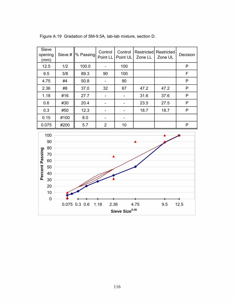
Development of Laboratory to Field Shift Factors for Hot-Mix Asphalt Resilient Modulus by Samer W. Katicha Thesis submitted to the Faculty of the Virginia Polytechnic Institute and State University In partial fulfillment of the requirements for the degree of Masters Of Science in Civil Engineering Imad L. Al-Qadi, Chair Gerardo Flintsch Amara Loulizi November 2003 Blacksburg, Virginia Keywords: resilient modulus, hot-mix asphalt, temperature, compaction Copyright by Samer W. Katicha 2003
Transcript
Development of Laboratory to Field Shift Factors for Hot-Mix Asphalt Resilient Modulus
by
Samer W. Katicha
Thesis submitted to the Faculty of the
Virginia Polytechnic Institute and State University
In partial fulfillment of the requirements for the degree of
1.4 Problem Statement and Research Objective................................................7 1.5 Scope................................................................................................................8
Chapter 2 Present State of Knowledge .........................................................9 2.1 Flexible Pavement and Their Main Design Factors......................................9
2.1.1 Input Design Parameters.........................................................................10 2.2 Material Characterization..............................................................................12
2.2.1 Resilient Modulus ....................................................................................13 2.2.2 Indirect Tension Test ...............................................................................14
2.3 Factors Affecting Resilient Modulus Results .............................................16 2.3.1 Mix Components Effect ...........................................................................16 2.3.2 Loading Effect..........................................................................................17 2.3.3 Effect of Poisson’s Ratio..........................................................................18 2.3.4 Effect of Testing Axis...............................................................................19 2.3.5 Specimen Size Effect ..............................................................................20 2.3.6 Effect of Measuring Devices....................................................................20 2.3.7 Effect of Moisture.....................................................................................22
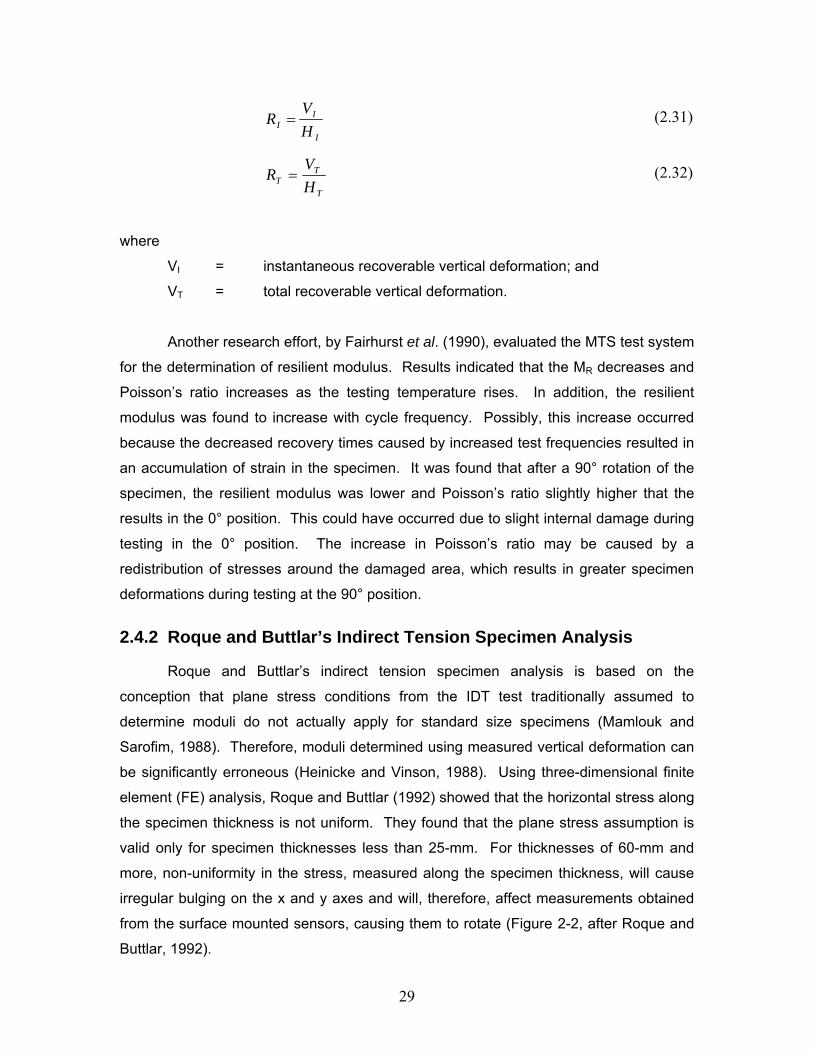
2.4 Resilient Modulus Data Analysis Methods .................................................23 2.4.1 Hondros’ 2-D Plane Stress Solution ........................................................23 2.4.2 Roque and Buttlar’s Indirect Tension Specimen Analysis .......................29 2.4.3 Three Dimensional Solution for the Indirect Tensile Test........................31
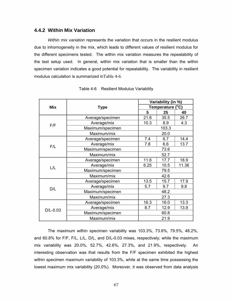
4.4.1 Within Specimen Variation ......................................................................66 4.4.2 Within Mix Variation.................................................................................67
Appendix A ......................................................................................................97
Appendix B ....................................................................................................142
Appendix C ....................................................................................................154
Vitae ....................................................................................................162
viii
List of Figures
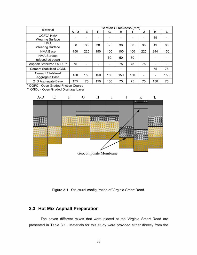
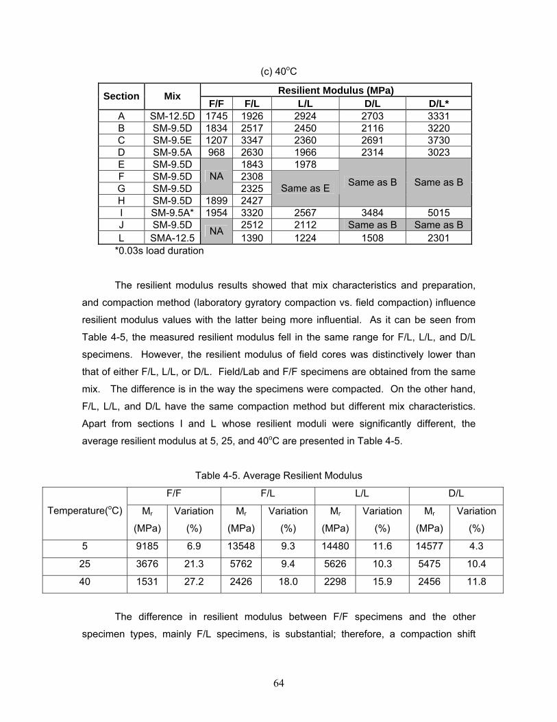
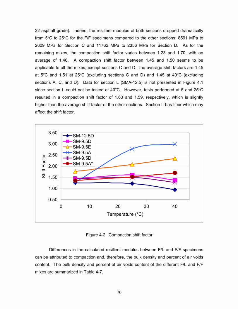
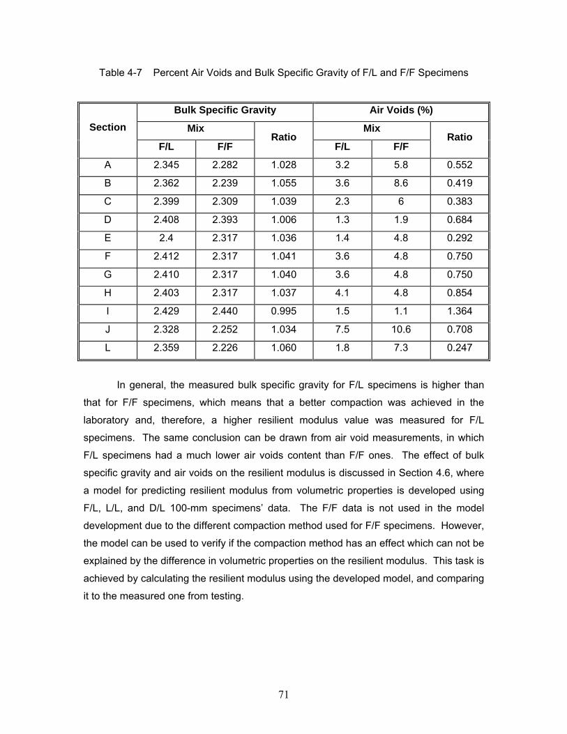
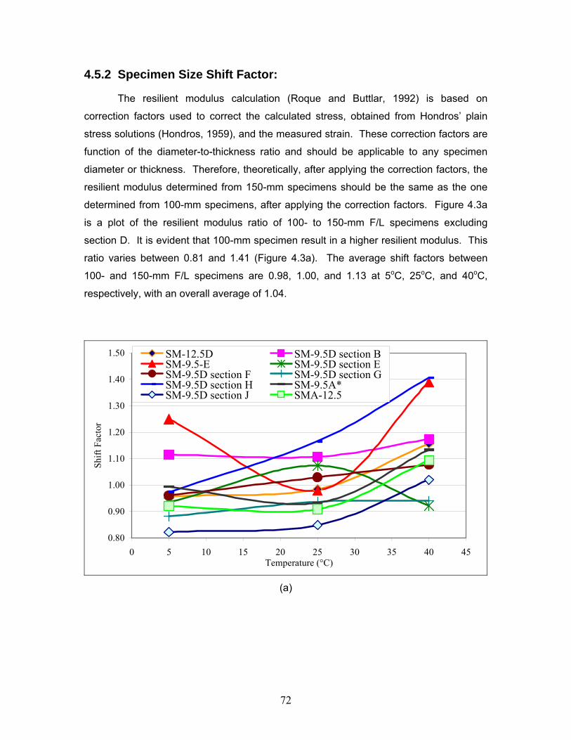
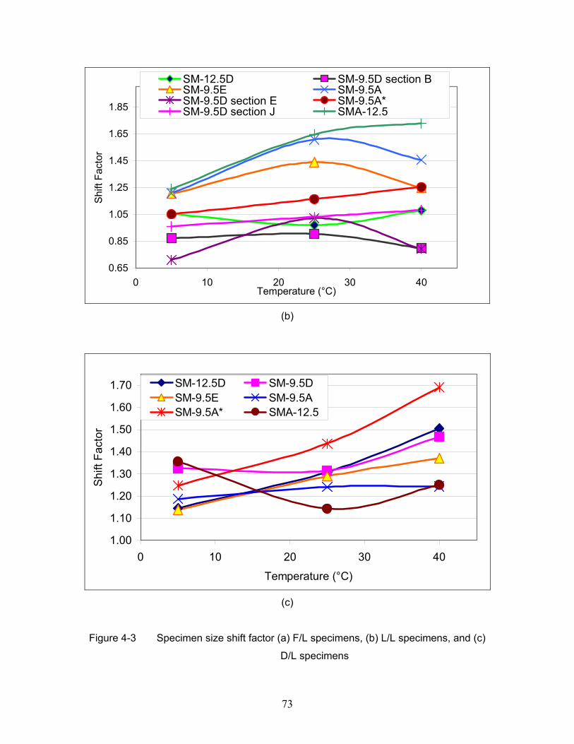
Figure 1-1 Flexible pavement cross-section. ..............................................................3 Figure 2-1 Elastic stress distribution in indirect tension specimen............................21 Figure 2-2 Illustration of Bulging Effects ...................................................................30 Figure 3-1 Structural configuration of Virginia Smart Road. .....................................37 Figure 3-2 Troxler Gyratory Compactor. ...................................................................41 Figure 3-3 Extensiometer Mounting..........................................................................43 Figure 3-4 Test configuration of the Indirect Tension Test .......................................44 Figure 3-5 Collected Data for Resilient Modulus Testing..........................................46 Figure 4-1 Stress Distribution ...................................................................................66 Figure 4-2 Compaction shift factor............................................................................70 Figure 4-3 Specimen size shift factor (a) F/L specimens, (b) L/L specimens, and (c)
D/L specimens ........................................................................................................73 Figure 4-4 Load Duration Shift Factor.......................................................................77 Figure 4-5 Resilient Modulus Variation with Temperature (Specimen A1-4in D/L)...79 Figure 4-6 Calculated vs. Measured Mr ....................................................................86
ix
List of Tables
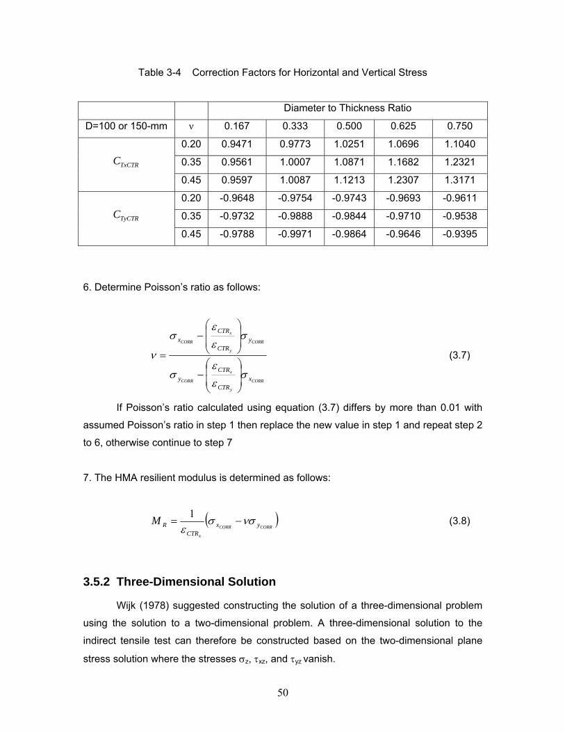
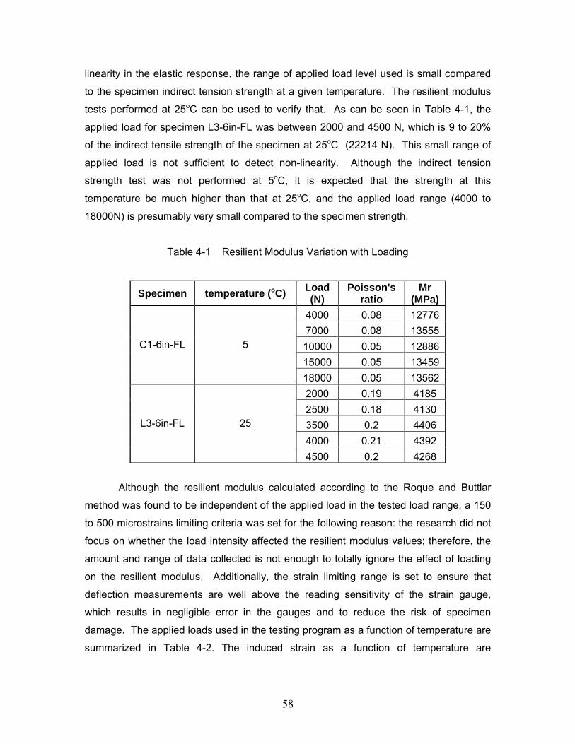
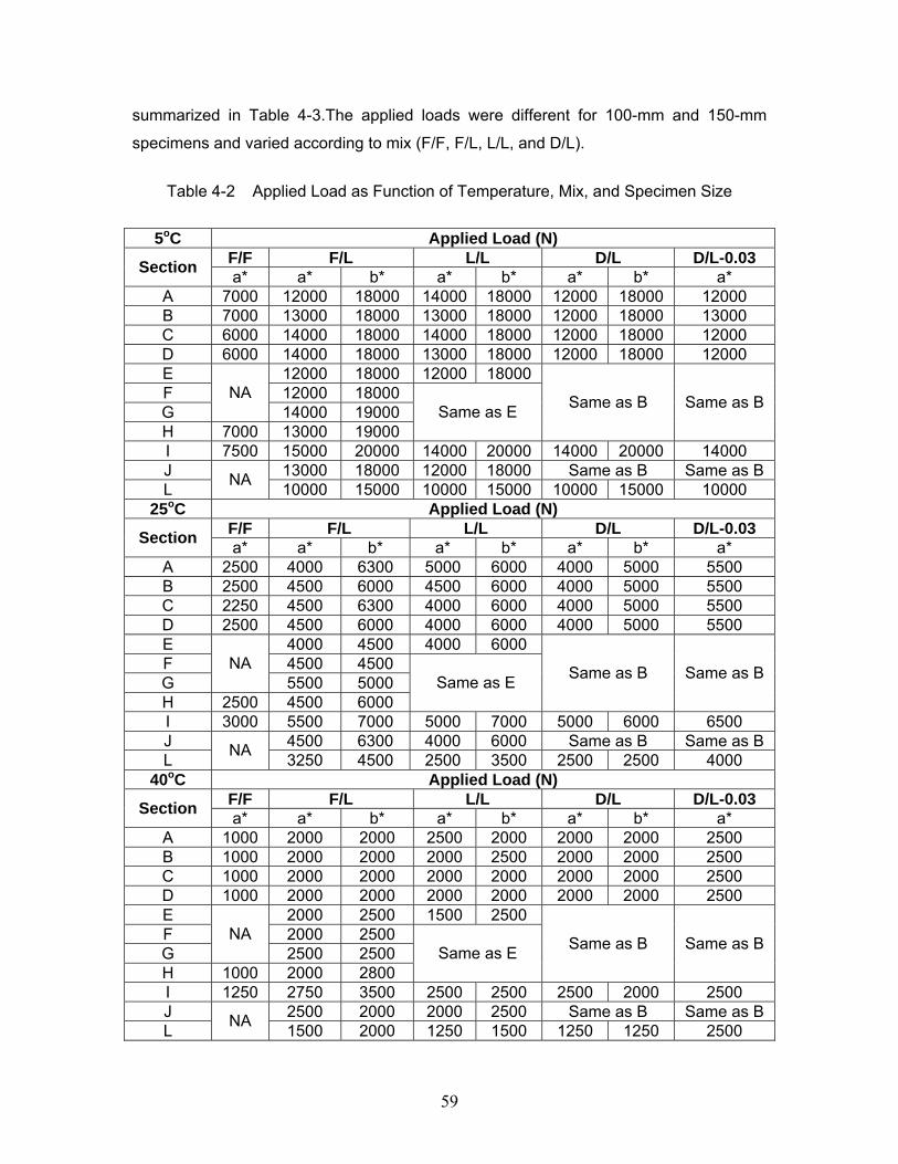
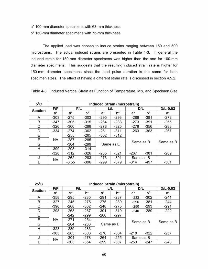
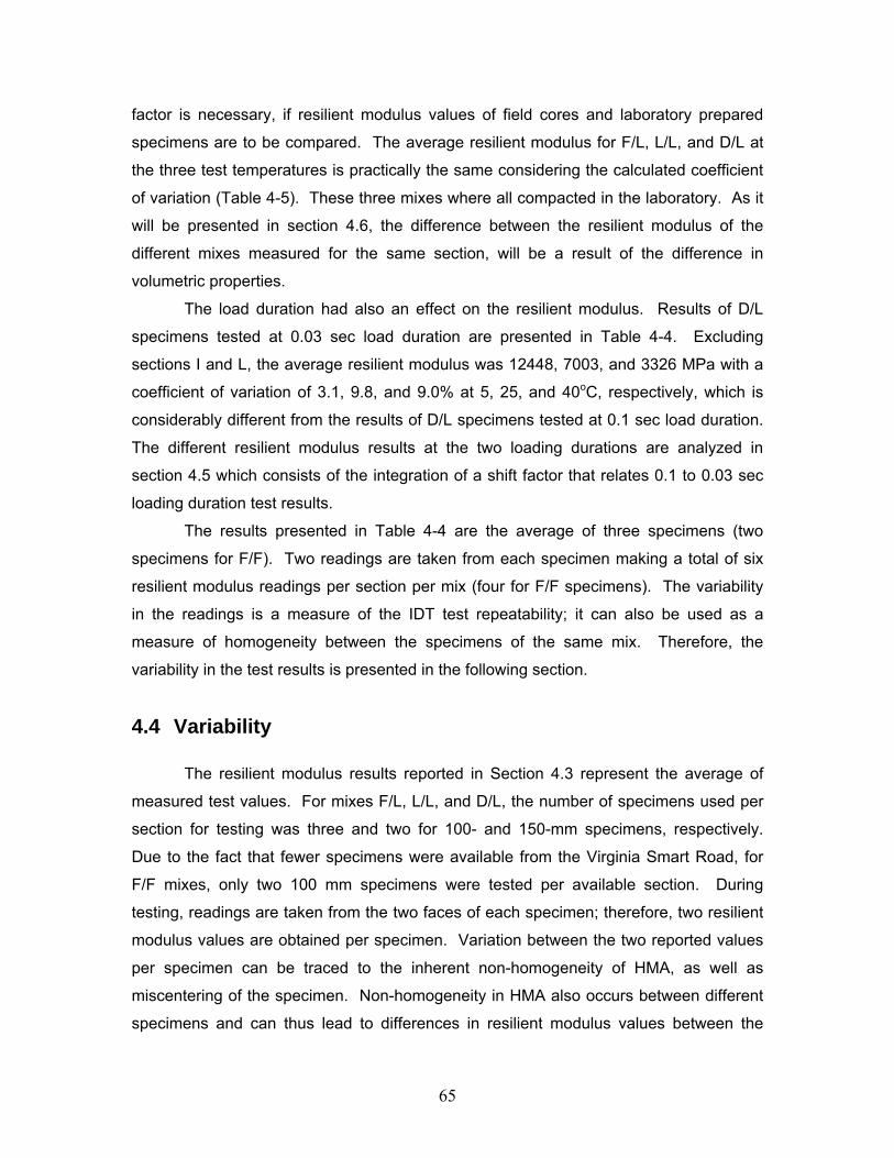
Table 3-1 Mixture characteristics at the Virginia Smart Road......................................38 Table 3-2 Number of Tested Specimens .....................................................................39 Table 3-3 Number of Gyrations for each Mix...............................................................42 Table 3-4 Correction Factors for Horizontal and Vertical Stress .................................50 Table 4-1 Resilient Modulus Variation with Loading....................................................58 Table 4-2 Applied Load as Function of Temperature, Mix, and Specimen Size..........59 Table 4-3 Induced Vertical Strain as Function of Temperature, Mix, and Specimen
Size 60 Table 4-4 Resilient Modulus Results for 100-mm Specimens at the Three Test
Temperatures..........................................................................................................63 Table 4-5. Average Resilient Modulus ............................................................................64 Table 4-6 Resilient Modulus Variability........................................................................67 Table 4-7 Percent Air Voids and Bulk Specific Gravity of F/L and F/F Specimens .....71 Table 4-8. t-statistic at: (a) 5oC, (b), 25oC, and (c) 40oC. ................................................76 Table 4-9 Values of α and β ........................................................................................80 Table 4-10 R2 Values for the Different Mixes.............................................................81 Table 4-11 Comparison between Calculated and Measured α and β .......................83 Table 4-12 Comparison between Calculated and Measured Resilient Modulus .......85 Table 4-13 Comparison between calculated and measured F/F resilient modulus ...87
1
Chapter 1 Introduction
In this chapter an overview of the pavement material characterization is
discussed. Hot mix asphalt (HMA) mixtures were tested to determine the creep
compliance, fatigue resistance, and resilient modulus of the different mixes which are
key input parameters in pavement design and rehabilitation. The characterization of
HMA depends on the way the material is obtained. This will lead to the formulation of
the problem statement, which will be followed by the research objectives. A summary of
the research scope is briefly presented at the end of the chapter.
1.1 Introduction
The Mechanistic-Empirical design of flexible pavements is based on limiting the
distresses in the pavement structure. Pavement distresses are caused by the different
types of loadings mainly structural and environmental loadings. Environmental loadings
are mainly addressed in the selection of the asphalt binder. The structural loading
distresses are mainly fatigue cracking and permanent deformation (rutting). Although
these two distresses are caused by the structural loading (vehicular loading on the
pavement structure), they are also affected by the environmental conditions. The
mechanistic-empirical pavement design method requires limiting the cracking and rutting
in the pavement structure. Many factors affect the ability of the HMA to meet these
structural requirements. These are the different components (aggregates and binders)
of the HMA, their interaction, the mix design, and the method of preparation. Great
efforts have been made to better understand HMA behavior. However, with the
increasing use of new technologies (e.g. modifiers in the binder, and reinforcement of
the pavement) and establishment of new design specifications, much work still needs to
be done to characterize HMA mixtures. Hot-mix asphalt mixes are primarily designed to
resist permanent deformation and cracking. The ability of the HMA to meet those
requirements depends on the following:
• The binder characteristics;
• Aggregate characteristics and gradation;
• Modifiers;
• Temperature;
• Moisture;
2
• Loading (load level, rate, and the loading rest time);
• Aging characteristics;
• State of stress (tension vs. compression, uniaxial, biaxial or Triaxial);
• Compaction method.
1.2 Background
1.2.1 Flexible Pavements
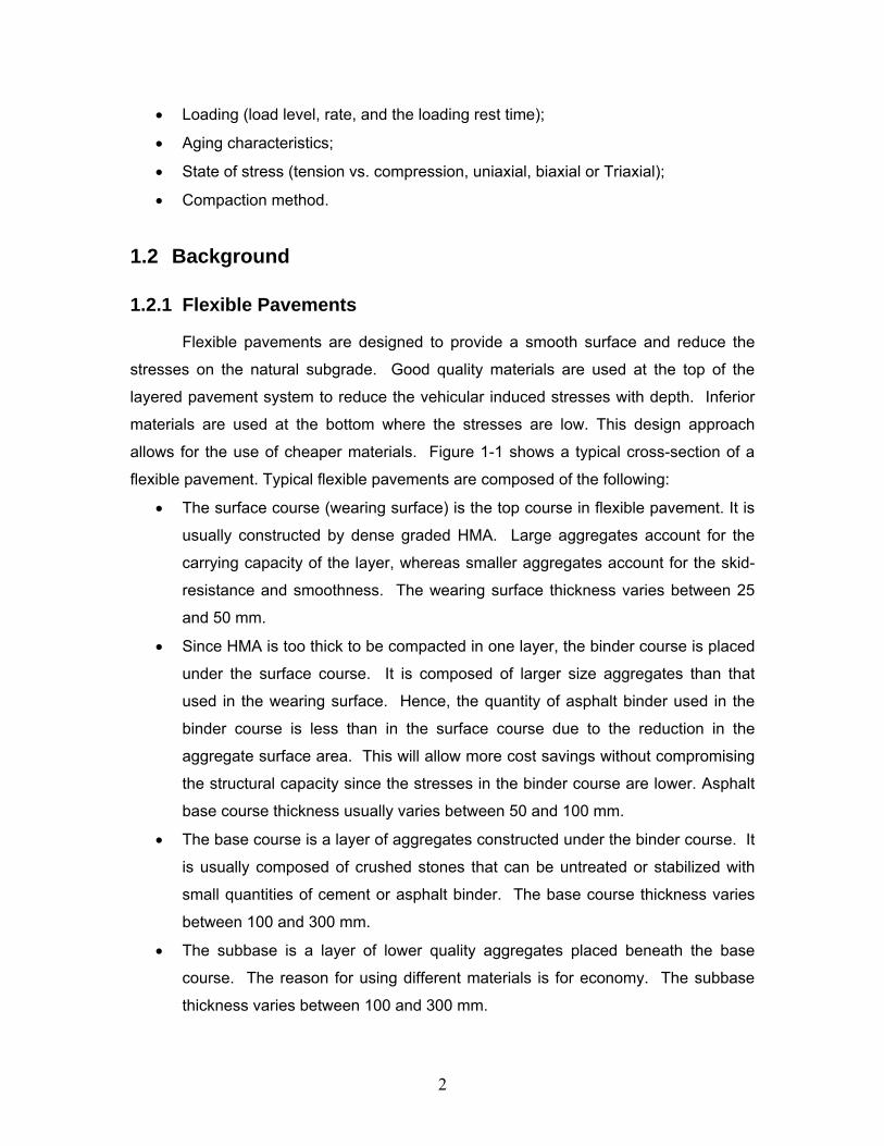
Flexible pavements are designed to provide a smooth surface and reduce the
stresses on the natural subgrade. Good quality materials are used at the top of the
layered pavement system to reduce the vehicular induced stresses with depth. Inferior
materials are used at the bottom where the stresses are low. This design approach
allows for the use of cheaper materials. Figure 1-1 shows a typical cross-section of a
flexible pavement. Typical flexible pavements are composed of the following:
• The surface course (wearing surface) is the top course in flexible pavement. It is
usually constructed by dense graded HMA. Large aggregates account for the
carrying capacity of the layer, whereas smaller aggregates account for the skid-
resistance and smoothness. The wearing surface thickness varies between 25
and 50 mm.
• Since HMA is too thick to be compacted in one layer, the binder course is placed
under the surface course. It is composed of larger size aggregates than that
used in the wearing surface. Hence, the quantity of asphalt binder used in the
binder course is less than in the surface course due to the reduction in the
aggregate surface area. This will allow more cost savings without compromising
the structural capacity since the stresses in the binder course are lower. Asphalt
base course thickness usually varies between 50 and 100 mm.
• The base course is a layer of aggregates constructed under the binder course. It
is usually composed of crushed stones that can be untreated or stabilized with
small quantities of cement or asphalt binder. The base course thickness varies
between 100 and 300 mm.
• The subbase is a layer of lower quality aggregates placed beneath the base
course. The reason for using different materials is for economy. The subbase
thickness varies between 100 and 300 mm.
3
• The subgrade is the bottom layer of compacted in-situ soil or selected material.
The subgrade should be compacted at the optimum moisture content to get a
high density.
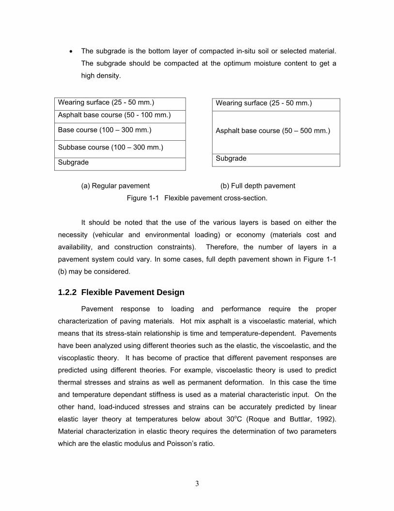
(a) Regular pavement (b) Full depth pavement
Figure 1-1 Flexible pavement cross-section.
It should be noted that the use of the various layers is based on either the
necessity (vehicular and environmental loading) or economy (materials cost and
availability, and construction constraints). Therefore, the number of layers in a
pavement system could vary. In some cases, full depth pavement shown in Figure 1-1
(b) may be considered.
1.2.2 Flexible Pavement Design
Pavement response to loading and performance require the proper
characterization of paving materials. Hot mix asphalt is a viscoelastic material, which
means that its stress-stain relationship is time and temperature-dependent. Pavements
have been analyzed using different theories such as the elastic, the viscoelastic, and the
viscoplastic theory. It has become of practice that different pavement responses are
predicted using different theories. For example, viscoelastic theory is used to predict
thermal stresses and strains as well as permanent deformation. In this case the time
and temperature dependant stiffness is used as a material characteristic input. On the
other hand, load-induced stresses and strains can be accurately predicted by linear
elastic layer theory at temperatures below about 30oC (Roque and Buttlar, 1992).
Material characterization in elastic theory requires the determination of two parameters
which are the elastic modulus and Poisson’s ratio.
Wearing surface (25 - 50 mm.)
Asphalt base course (50 - 100 mm.)
Base course (100 – 300 mm.)
Subbase course (100 – 300 mm.)
Subgrade
Wearing surface (25 - 50 mm.)
Asphalt base course (50 – 500 mm.)
Subgrade
4
The elastic modulus has been traditionally determined in the field using deflection
obtained from non destructive tests such as the Falling Weight Deflectometer (FWD).
However, moduli determined through back calculation are for a specific temperature at
which the test was performed. Although generalized relationships between HMA elastic
modulus and temperature have been developed, their use can lead to considerable error
since these relationships can vary between one asphalt mix and another. Moreover, it
has been shown that near surface layer moduli determined using deflection basins from
FWD testing are not accurate. These problems can be overcome in the laboratory
where materials from each layer can be tested at a controlled temperature. Material
properties determined in the laboratory can vary considerably from one test setup to
another. Proper material properties are obtained when the laboratory setup induces
stress states that are similar to the ones experienced in the filed.
Testing in the lab can be performed on field specimens or laboratory-produced
specimens. Differences have been shown to exist between field and laboratory-
produced specimens using different methods of compaction. Gyratory compaction has
been proven to better correlate with field compaction than other methods (Button et al.,
1994). The gyratory compaction is the one used in the Superpave design protocol, and
will be used in the following research.
1.2.3 Failure Criteria in Flexible Pavements
Fatigue Cracking:
Fatigue cracking of flexible pavements is thought to be based on the horizontal
tensile strain at the bottom of the HMA layer. The failure criterion relates the allowable
number of load repetitions to the tensile strain. The cracking initiates at the bottom of
the HMA where the tensile strain is highest under the wheel load. The cracks propagate
initially as one or more longitudinal parallel cracks. After repeated heavy traffic loading,
the cracks connect in a way resembling the skin of an alligator. Laboratory fatigue tests
are performed on small HMA beam specimens. Due to the difference in geometric and
loading conditions; especially rest period between the laboratory and the field, the
allowable number of repetitions for actual pavements is greater than that obtained from
laboratory tests. Therefore, the failure criterion may require incorporating a shift factor to
account for the difference.
5
Rutting:
Rutting is indicated by the permanent deformation along the wheelpath. Rutting
can occurs in any of the pavement layers or the subgrade, usually caused by the
consolidation or the lateral movement of the materials due to traffic loads. Rutting in the
HMA layer is controlled by the creep compliance of the mix. Rutting occurring in the
subgrade is caused by the vertical compressive strain at the top of the subgrade layer.
To control rutting occurring in the subgrade, the vertical compressive strain at the top of
the subgrade is limited to a certain value.
It is noticed that fatigue cracking and rutting depend on the level of strain; tensile
strain at the bottom of the HMA layer for fatigue cracking, and compressive strain at the
top of the subgrade layer for rutting. Therefore, to be able to predict the fatigue as well
as the rutting lives of the pavement structure, the aforementioned strains must be
determined. Load induced stresses and strains in pavements are determined using the
elastic layered theory. This requires the determination of the moduli of the different
layers in the pavement structure. Moduli are usually determined in the field by
performing the FWD test. However, near surface moduli (modulus of the wearing
surface) are difficult to obtain using FWD results. Moreover, for the design of the
pavement, layers moduli must be determined prior to the pavement is construction.
1.3 Material Characterization
Hot mix asphalt can be characterized as either a viscoelastic or an elastic
material. Viscoelastic characterization involves measuring the dynamic complex
modulus and the creep compliance. Elastic characterization involves measuring the
resilient modulus. Since HMA’s properties are functions of time and temperature, its
characterization should reflect this fact.
1.3.1 Dynamic Complex Modulus
The dynamic complex modulus has been used for the design of pavements
(Shook, 1969). The complex modulus test performed in the laboratory by applying a
sinusoidal or haversine loading with no rest period. This testing approach is one of
many methods for describing the stress-strain relationship of viscoelastic materials. The
dynamic complex modulus is composed of two parts: the real part, which represents the
elastic stiffness and the imaginary part, which represents the internal damping due to the
6
viscoelastic properties of the material. The absolute value of the complex modulus is
referred to as the dynamic modulus of HMA. The axial strains are measured using two
strain gauges. The ratio between the axial stress and the recoverable strain is the
dynamic elastic modulus. The dynamic complex modulus is determined from the
dynamic modulus and the phase angle. The phase angle being the lag between the
stress and strain maximum values.
The dynamic complex modulus test, ASTM D3497-79 (ASTM, 2003), is usually
conducted on cylindrical specimens subjected to a compressive haversine loading
varying with the loading frequency. The testing mode selected will have an effect on the
design if the design is based on the viscoelastic theory; in such a case the loading and
frequency should be selected such that it best simulates the traffic loading. Most of the
dynamic modulus tests use a compressive load applied to the specimen. However,
other tests have also been used such as the tension and tension-compression tests. A
haversine load is applied to the specimen for a minimum of 30s not exceeding 45s at
temperatures of 5, 25, and 40oC and a load frequency of 1, 4, and 16 Hz for each
temperature.
The test is affected by the setup and the effect becomes more prominent at
higher temperatures. Therefore if a design is based on elastic theory with a given
dynamic modulus for HMA, the three different testing temperature results may be used.
1.3.2 Resilient Modulus
The resilient modulus is the elastic modulus used in the layered elastic theory for
pavement design. Hot mix asphalt is known to be a viscoelstic material and, therefore,
experiences permanent deformation after each application of the load. However, if the
load is small compared to the strength of the material and after a relatively large number
of repetitions (100 to 200 load repetitions), the deformation after the load application is
almost completely recovered. The deformation is proportional to the applied load and
since it is nearly completely recovered it can be considered as elastic.
The resilient modulus is based on the recoverable strain under repeated loading and is
determined as follows:
r
drM
εσ
=
7
where σd is the deviator stress and εr is the recoverable (resilient strain). Because the
applied load is usually small compared to the strength of the specimen, the same
specimen may be used for the same test under different loading and temperatures.
The resilient modulus is evaluated from repeated load tests. Different types of
repeated load tests have been used to evaluate the resilient modulus of HMA. The most
commonly used setups are the uniaxial tension, the uniaxial compression, the beam
flexure, the triaxial compression, and the indirect diametral tension (IDT). The IDT setup
has a main advantage in its ability to simulate the stress states that exist at the bottom of
the HMA layer underneath the applied wheel load, which are of concern in pavement
design. The state of stress in an IDT specimen is rather complex, however extensive
research has been performed to address this subject, and data analysis methods are
available to accurately predict stresses and strains (Roque and Buttlar, 1992; Kim, et al.,
2002).
The resilient modulus can be performed on laboratory prepared specimens or
field cores. For consistency in design, results obtained from laboratory prepared
specimens should match with results obtained from field cores.
1.3.3 Creep Compliance
The creep test is used to characterize linear viscoelastic materials. Viscoelastic
materials such as hot mix asphalt experience an increase in total deformation as the
applied load is sustained. This phenomenon is time and temperature dependent. The
creep compliance is defined as the ratio of the instantaneous strain over the applied
stress. Creep testing is used to characterize permanent deformation. Test setups that
have been used are uniaxial (Van de Loo, 1978) and more recently indirect tension
(Roque and Buttlar, 1992; Buttlar and Roque, 1994; Wen and Kim, 2002; Kim, et al.,
2002). The advantages and disadvantages of the IDT setup for creep testing are the
same as for resilient modulus testing.
Specimen compaction is an important parameter that affects the dynamic
modulus, resilient modulus, and creep compliance laboratory results.
1.4 Problem Statement and Research Objective
Gyratory compaction was introduced by the Strategic Highway Research
Program (SHRP) as the compaction method that best replicates compaction performed
8
in the field. However, correlation between laboratory compacted HMA specimens
properties and field compacted HMA properties are not well established. Discrepancies
between laboratory prepared specimens and field cores are not solely due to
compaction; differences between the designed and as built mixes system can be quiet
significant. Specimens in the laboratory can be prepared to conform to the designed or
the as built pavement. Therefore, the development of correction factors between
laboratory-prepared specimens and specimens obtained from the field will provide
valuable information for adjusting design procedures. Hence, better prediction of
pavement performance can be achieved.
The main objective of this research was to develop shift factors to correlate
laboratory-determined resilient moduli of field cores to those of laboratory-prepared
specimens. These factors could be dependent on compaction method, specimen size,
temperature, mix production, and loading.
1.5 Scope
This research attempted to quantify the variations in resilient modulus results due
to different parameters. These parameters are specimen size, load pulse duration,
temperature, and method of production and compaction. The most important task was
to develop shift factors to relate resilient modulus of laboratory-prepared specimens to
resilient modulus of field cores. Chapter 1 is an introduction to the subject. Chapter 2
presents an overview of the present stage of knowledge regarding resilient modulus
testing and the parameters affecting its values. The resilient modulus results depend
on the analysis method used. The analysis method used should be the one that gives
the best representation of the state of stress in the specimen. The different analysis
methods available are discussed in chapter 2. In Chapter 3 the research approach is
outlined and details on specimen preparation, testing, and analysis of the results are
presented. The material used were obtained either directly from the Virginia Smart
Road, in form of road cores or loose-bagged mixture samples collected during
construction, or were produced in the laboratory from raw materials to meet design
specifications. The research results and interpretation are presented in Chapter 4.
Finally, the conclusions and recommendations are presented in Chapter 5. The research
21B Aggregate Base 175 75 150 150 75 75 75 150 75* OGFC - Open Graded Friction Course** OGDL - Open Graded Drainage Layer
Material Section / Thickness (mm)
38
Virginia Smart Road, in the form of road cores or loose bagged mixture samples
collected during construction, or were produced from raw materials to meet either
volumetric criteria determined from road cores or to meet design specifications. All raw
materials used for production of specimens were obtained from the source utilized
during construction. Practices recommended by the Virginia Department of
Transportation and in accordance with Superpave protocol were implemented in
specimen preparation.
Table 3-1 Mixture characteristics at the Virginia Smart Road
Section HMA Wearing Surface Characteristics
A SM-12.5D 12.5mm nominal maximum aggregate size
PG 70-22 binder
B, E – H, J SM-9.5D 9.5mm nominal maximum aggregate size
PG 70-22 binder
C SM-9.5E 9.5mm nominal maximum aggregate size
PG 76-22 binder
D, I SM-9.5A
9.5mm nominal maximum aggregate size
PG 64-22 binder
Section I designed with high lab compaction
K OGFC 12.5mm nominal maximum aggregate size
PG 76-22 binder
L SMA-12.5 12.5mm nominal maximum aggregate size
PG 76-22 binder
3.3.1 Specimen Designation and Characteristics
Three specimen types were produced in two different sizes; 100-mm diameter
specimens and 63.5-mm thick and 150-mm diameter specimens and 76.2-mm thick. A
fourth specimen type was obtained from the Virginia Smart Road in form of 100-mm
diameter field cores. The thickness of the field cores was controlled by the thickness of
the constructed HMA layer. The four specimen types are divided into the following
categories:
39
• Field/field (F/F): field cores from the Virginia Smart Road, only available in 100-
mm diameter. Field core thickness is controlled by the wearing thickness at the
Virginia Smart Road and varied between 37 and 50 mm;
• Field/lab (F/L): specimens compacted in the laboratory from loose mixtures
samples obtained from the field at the time of construction;
• Lab/lab (L/L): specimens produced and compacted in the laboratory using
volumetric results from field specimens; and
• Design/lab (D/L): specimens produced and compacted in the laboratory
according to design specifications.
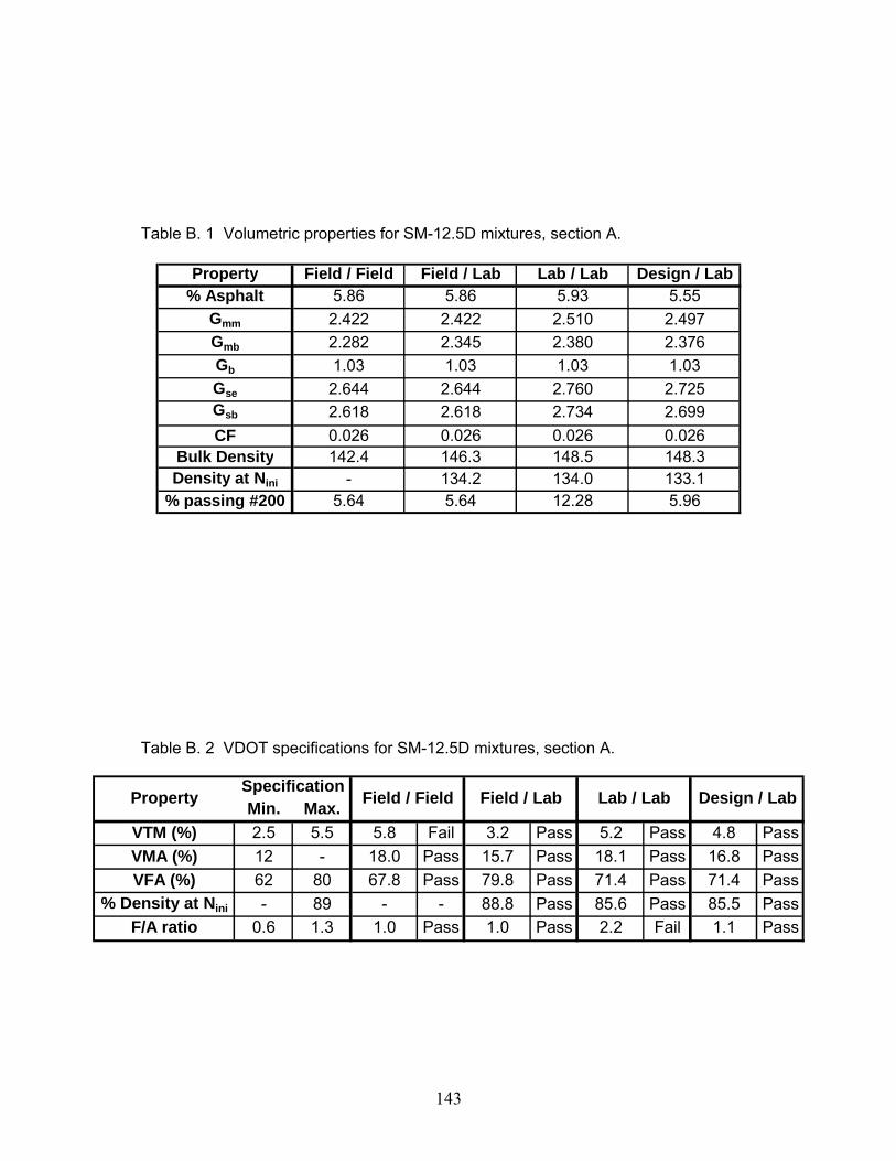
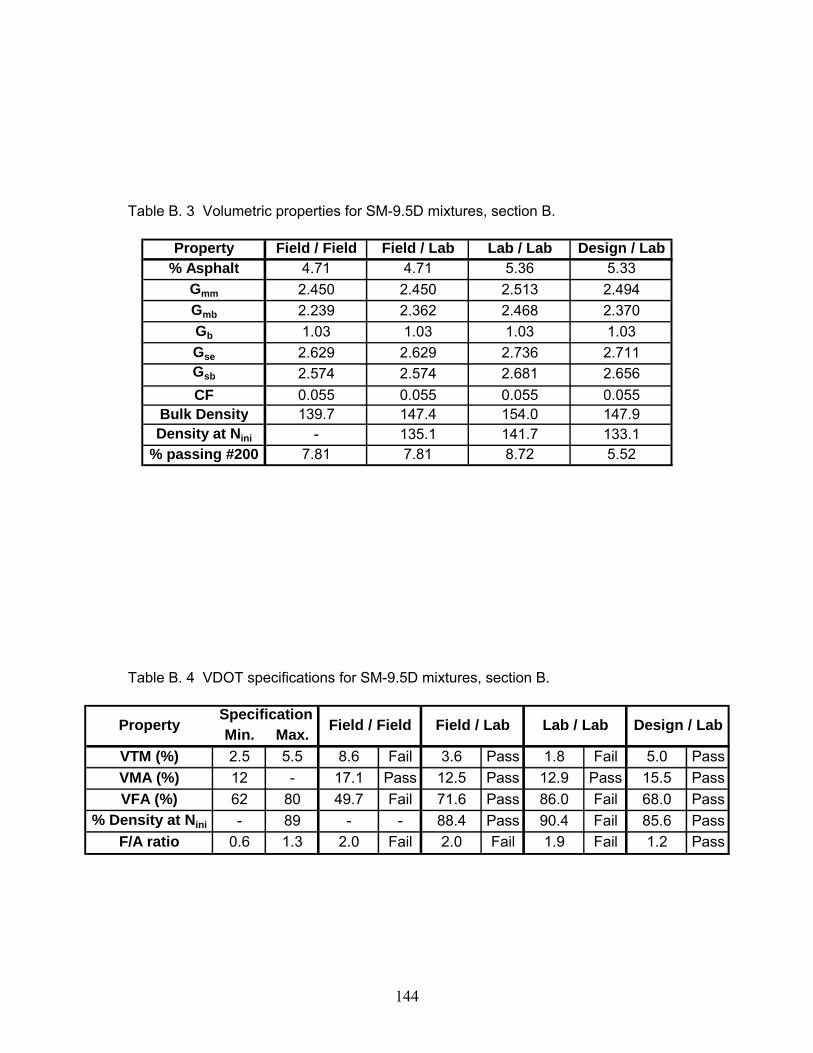
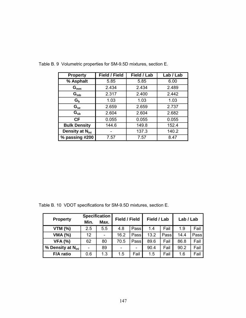
The analysis of volumetric properties was performed for all mixtures. It included
specimen bulk specific gravity and compaction densification curves, mixture maximum
theoretical specific gravity (Rice), aggregate gradation, and asphalt content
measurements for the four different types of mixes. The results are presented in
Appendices A and B. The Summary of the tests specimens for resilient modulus
evaluation is presented in Table 3-2.
Table 3-2 Number of Tested Specimens
Section Mixture F/F F/L L/L D/L* a a b a b a b A SM12.5D 2 3 2 3 2 6 2 B SM-9.5D 2 3 2 3 2 6 2 C SM-9.5E 2 3 2 3 2 6 2 D SM-9.5A 2 3 2 3 2 6 2 E SM-9.5D 2 3 2 3 2 F SM-9.5D 2 3 2 G SM-9.5D 2 3 2 H SM-9.5D 2 3 2
Same as E Same as B
I SM-9.5A* 2 3 2 3 2 6 2 J SM-9.5D 2 3 2 3 2 Same as B K OGFC Not tested L SM-12.5 2 3 2 3 2 6 2
D/L* 3 specimens tested at 0.1 sec load pulse and 3 specimens tested at 0.03 sec
load pulse
a 100-mm diameter specimens with 63-mm thickness
b 150-mm diameter specimens with 75-mm thickness
40
3.3.2 Specimen Preparation
Field/Field Specimens
F/F specimens consist of cores obtained from the Virginia Smart Road wearing
surface. After core extraction, the wearing surface was separated from the base mix
(BM). The extracted samples’ surfaces had to be treated so that they are smooth
enough to mount the extensiometers. The specimen thickness was recorded as the
average of three measurements taken at 120o intervals.
Field/Lab Specimens
Field/Lab mixes were collected during the construction of the Virginia Smart
Road. Samples were heated to be brought up to compaction temperature. This
procedure was performed in less than an hour to prevent specimen aging. The
specimens were then compacted using a troxler gyratory compactor. The compaction
temperature ranged between 135 and 144oC. The specimens volumetric properties
were then taken before they were cut to the specified thickness (63.5- and 76.2-mm for
100- and 150-mm specimens respectively) to be tested.
Lab/Lab Specimens
Lab/Lab mixes were produced in the laboratory to replicate F/L mixes.
Aggregate gradation and asphalt content were determined by from F/L mixes, using the
ignition oven for asphalt content determination. Lab/Lab gradations were designed to
replicate as closely as possible F/L gradations by mixing the proper amount of the
different aggregate types used for the construction of the Virginia Smart Road. The
proper amount of asphalt binder was then added to the aggregate for mixing. The
mixing temperature ranged between 135 and 170oC. The procedure for compaction and
final sample preparation was the same as for F/L specimens.
Design/Lab Specimens
The procedure for preparing D/L specimens was the same as the one for L/L
specimens except that the aggregate gradation and asphalt content are determined from
the design sheets.
41
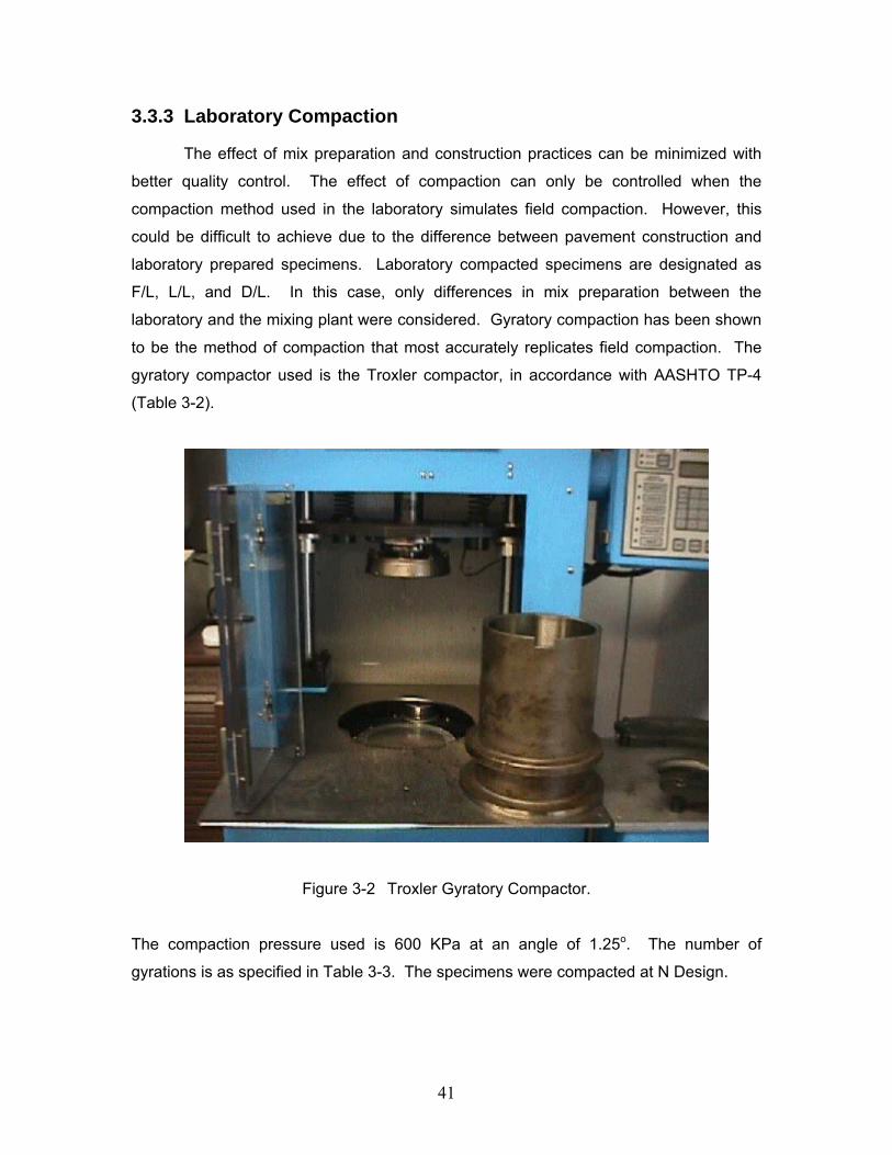
3.3.3 Laboratory Compaction
The effect of mix preparation and construction practices can be minimized with
better quality control. The effect of compaction can only be controlled when the
compaction method used in the laboratory simulates field compaction. However, this
could be difficult to achieve due to the difference between pavement construction and
laboratory prepared specimens. Laboratory compacted specimens are designated as
F/L, L/L, and D/L. In this case, only differences in mix preparation between the
laboratory and the mixing plant were considered. Gyratory compaction has been shown
to be the method of compaction that most accurately replicates field compaction. The
gyratory compactor used is the Troxler compactor, in accordance with AASHTO TP-4
(Table 3-2).
Figure 3-2 Troxler Gyratory Compactor.
The compaction pressure used is 600 KPa at an angle of 1.25o. The number of
gyrations is as specified in Table 3-3. The specimens were compacted at N Design.
42
Table 3-3 Number of Gyrations for each Mix
Number of Gyrations Section
HMA Wearing
Surface N Design N Initial N max
A SM-12.5D 75 7 115
B, E – H, J SM-9.5D 75 7 115
C SM-9.5E 75 7 115
D, I SM-9.5A 65 7 100
K OGFC Not Tested
L SMA-12.5
Prior to compaction, the HMA and the mold were heated to the specified compaction
temperature. When compaction was completed, the specimens were allowed to cool
down before being extracted from the mold, which would reduce the possibility of
inducing residual stresses on the specimen sides. The volumetric properties were then
measured before cutting the samples to the specified thickness for testing.
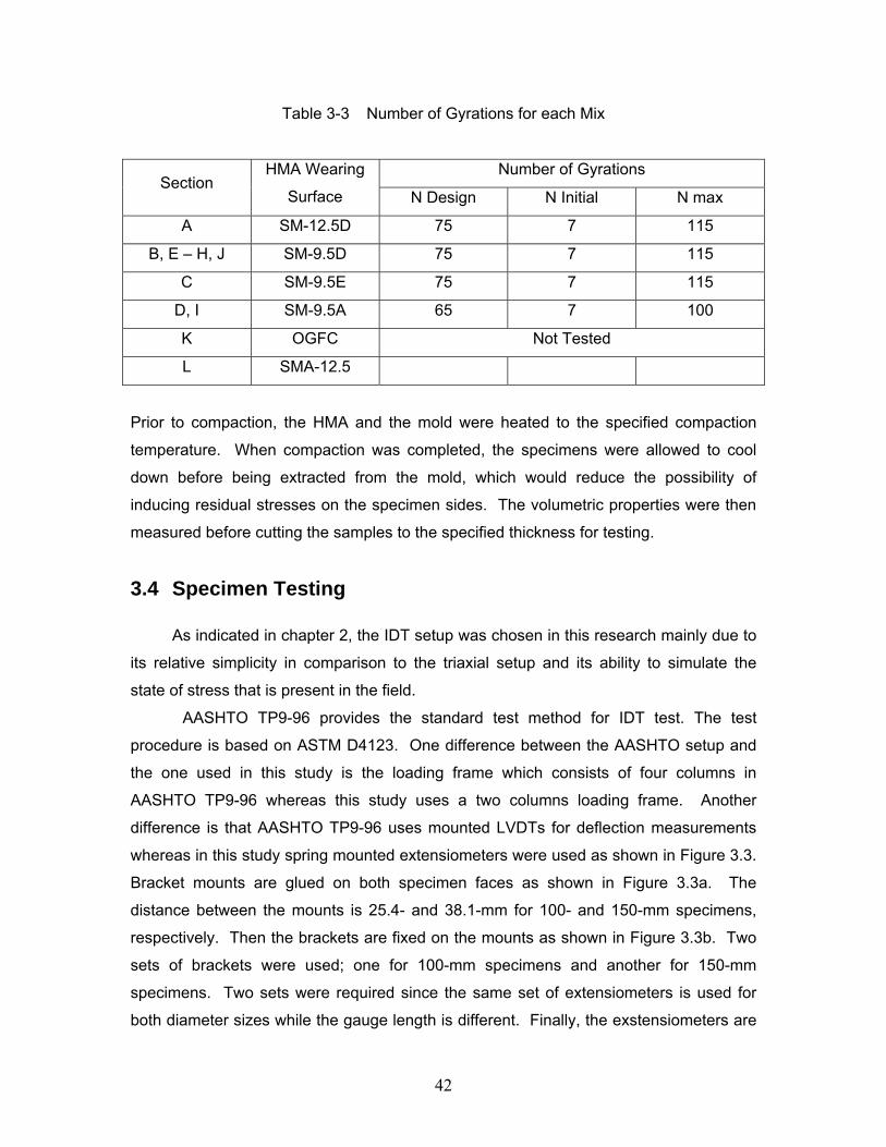
3.4 Specimen Testing
As indicated in chapter 2, the IDT setup was chosen in this research mainly due to
its relative simplicity in comparison to the triaxial setup and its ability to simulate the
state of stress that is present in the field.
AASHTO TP9-96 provides the standard test method for IDT test. The test
procedure is based on ASTM D4123. One difference between the AASHTO setup and
the one used in this study is the loading frame which consists of four columns in
AASHTO TP9-96 whereas this study uses a two columns loading frame. Another
difference is that AASHTO TP9-96 uses mounted LVDTs for deflection measurements
whereas in this study spring mounted extensiometers were used as shown in Figure 3.3.
Bracket mounts are glued on both specimen faces as shown in Figure 3.3a. The
distance between the mounts is 25.4- and 38.1-mm for 100- and 150-mm specimens,
respectively. Then the brackets are fixed on the mounts as shown in Figure 3.3b. Two
sets of brackets were used; one for 100-mm specimens and another for 150-mm
specimens. Two sets were required since the same set of extensiometers is used for
both diameter sizes while the gauge length is different. Finally, the exstensiometers are
43
mounted on the brackets (Figure 3.3c). The specimen diameter to gauge length ratio is
the same for both specimen sizes. The gauge length is set at 25.4-mm for 100-mm
diameter specimens as specified in AASHTO TP9-96. The gauge length for the 150-mm
diameter specimens is 38.1-mm. The gauge length chosen is important to minimize the
possibility of placing the gauge in a zone primarily influenced by a single aggregate. A
minimum of 25.4 mm gauge length is, therefore, required for 100-mm diameter
specimens and was used by Roque and Buttlar (1992), Ruth and Maxfield (1977),
Anderson and Hussein (1990), and Hugo and Nachenius (1989). Also, a gauge of 25.4-
mm for 100-mm specimens and 38.1-mm for 150mm specimens will ensure that
deflections are measured over an area of relatively uniform stress distribution as
suggested by Roque and Buttlar (1992).
a) Glued mount b) Brackets
c) Extensiometers
Figure 3-3 Extensiometer Mounting
44
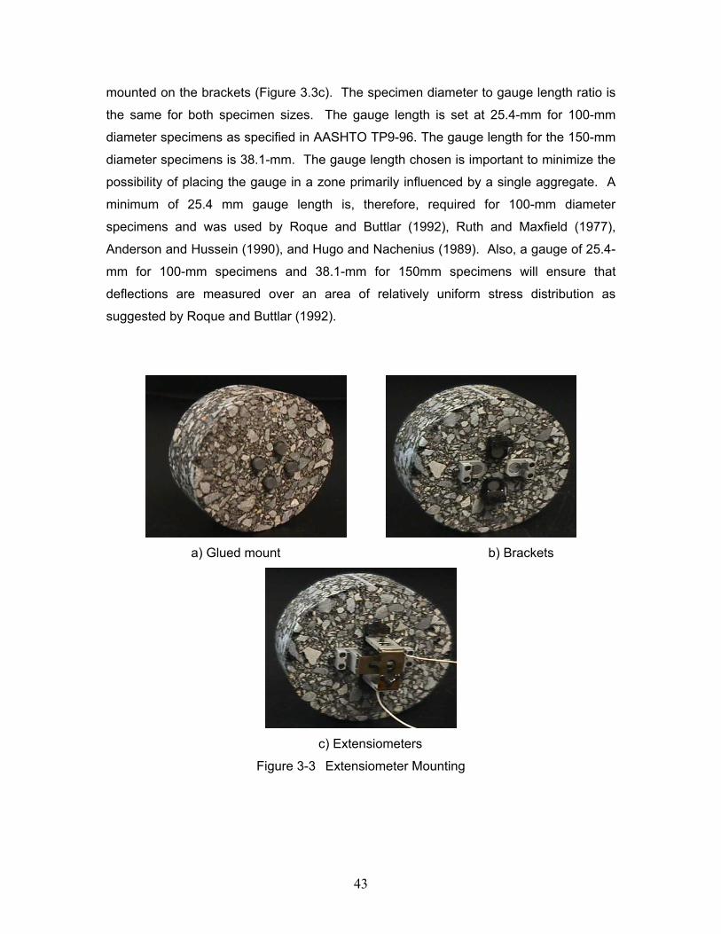
The IDT test was performed using an MTS servo-hydraulic closed-loop testing
machine. An environmental chamber was used to control the temperature of the
specimens. Specimens were conditioned for 24hrs for 5 and 25oC and at least 3 to 6hrs
for 40oC testing. Applied loads were measured by the MTS load cell calibrated for
8900N, 22200N, and 89000N. The 8900N calibration was used for resilient modulus
testing at 25oC and 40oC, while the 22000N calibration was used for resilient modulus
testing at 5oC. The 89000N calibration was used for the indirect tensile strength test
(IDTST). Deflection measurements were taken at both specimen surfaces to evaluate
the within specimen variation. The test configuration of the IDT test is shown in Figure
3-4.
Figure 3-4 Test configuration of the Indirect Tension Test
45
3.4.1 Loading
The applied load was selected in a way to limit the strain between 150 and 500
microstrain. The upper limit of 500 microstrain was set to prevent specimen damage as
recommended by Roque and Buttlar (1994), whereas the lower limit of 150 microstrain is
set to obtain measurements much higher than the LVDTs’ sensitivity. In this study, the
150 microstrain criterion was used after it was found that the signal to noise ratio of the
extensiometers, at this range of strains, was very high. Hence, the applied load varied
between mixes design and specimen sizes. The load used is a haversine load of 0.1
sec pulse duration and 0.9 sec rest period for all the specimens. A second set of D/L
specimens was tested at a load of 0.03 sec pulse duration and 0.97 rest period as
suggested by Loulizi et al. (2002). Since the load was not known a priori, many tests
were performed on the first specimen of each section to define the appropriate loading.
The initial applied load was relatively small to prevent damaging the specimen. The
specimen was allowed to recover for a period of 30mins before it was tested again under
a different loading. The load at which the measured horizontal and vertical deformations
fell in the range of 150 and 500 microstrain was the load used to test the rest of the
specimens. This same procedure was repeated for each mix at the three different
temperatures (5, 25, and 40oC). The final loads used for testing are presented in
Chapter 4.
3.4.2 Testing and Data Collection
The IDT test for the resilient modulus was conducted at 100 cycles for all testing
temperatures. After 100 cycles, the accumulated plastic strain per cycle becomes
negligible. The 100 conditioning cycles simulate the consolidation that occurs in
pavements when it is opened for traffic. Deflection and load readings were recorded for
the last 5 cycles of the test at 0.0048828 sec intervals. The readings were averaged to
determine the resilient modulus and Poisson’s ratio. The calculated resilient modulus
variation in any two loading cycles has to be lower than 5% for test results acceptance.
Two resilient modulus and Poisson’s ratio values were determined for every specimen;
one at each specimen’s surface. An example of the collected data is presented in figure
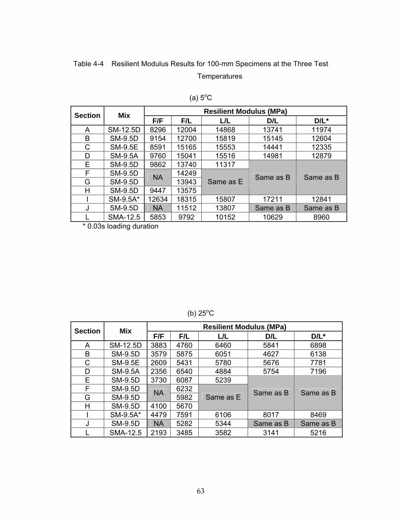
A SM-12.5D 8296 12004 14868 13741 11974 B SM-9.5D 9154 12700 15819 15145 12604 C SM-9.5E 8591 15165 15553 14441 12335 D SM-9.5A 9760 15041 15516 14981 12879 E SM-9.5D 9862 13740 11317 F SM-9.5D 14249 G SM-9.5D NA 13943 H SM-9.5D 9447 13575
Same as E Same as B Same as B
I SM-9.5A* 12634 18315 15807 17211 12841 J SM-9.5D NA 11512 13807 Same as B Same as B L SMA-12.5 5853 9792 10152 10629 8960
A SM-12.5D 3883 4760 6460 5841 6898 B SM-9.5D 3579 5875 6051 4627 6138 C SM-9.5E 2609 5431 5780 5676 7781 D SM-9.5A 2356 6540 4884 5754 7196 E SM-9.5D 3730 6087 5239 F SM-9.5D 6232 G SM-9.5D NA 5982 H SM-9.5D 4100 5670
Same as E Same as B Same as B
I SM-9.5A* 4479 7591 6106 8017 8469 J SM-9.5D NA 5282 5344 Same as B Same as B L SMA-12.5 2193 3485 3582 3141 5216
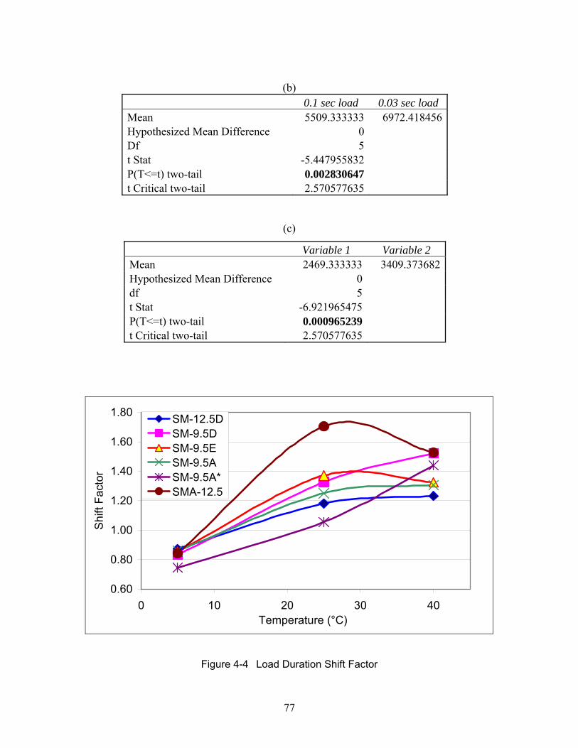
0.1 sec load 0.03 sec load Mean 14358 11932 Hypothesized Mean Difference 0 df 5 P(T<=t) two-tail 0.001935352 t Critical two-tail 2.570577635
77
(b)
0.1 sec load 0.03 sec load Mean 5509.333333 6972.418456 Hypothesized Mean Difference 0 Df 5 t Stat -5.447955832 P(T<=t) two-tail 0.002830647 t Critical two-tail 2.570577635
(c)
Variable 1 Variable 2 Mean 2469.333333 3409.373682 Hypothesized Mean Difference 0 df 5 t Stat -6.921965475 P(T<=t) two-tail 0.000965239 t Critical two-tail 2.570577635
0.60
0.80
1.00
1.20
1.40
1.60
1.80
0 10 20 30 40Temperature (°C)
Shi
ft Fa
ctor
SM-12.5DSM-9.5DSM-9.5ESM-9.5ASM-9.5A*SMA-12.5
Figure 4-4 Load Duration Shift Factor
78
However, results of tests performed at 5oC produced a shift factor lower than 1
for all the tested sections, which would indicate that the measured strain induced by a
load sustained for a shorter period of time is higher than the one induced by the same
load sustained for a longer period of time, which is theoretically and practically
impossible. The explanation for a shift factor smaller than unity is related to the IDT test
execution. The resilient modulus test is a repetitive loading test. Hot-mix asphalt
experiences an accumulation of plastic strain during repetitive loading. However, the
accumulated plastic strain decreases with every new loading cycle and eventually
becomes negligible. The accumulated plastic strain per cycle is a function of the load
duration and increases with longer load durations. The resilient modulus test was run for
100 cycles for both loading durations, which may lead to a higher total accumulated
plastic strain for specimens tested for longer load durations. It is, therefore, possible that
the accumulated strain per cycle for specimens tested at shorter load durations will still
be significant and that those specimens need additional conditioning cycles, which will
lead to lower resilient moduli. The load duration shift factors varied between 0.75 and
0.87, 1.06 and 1.70, 1.23 and 1.53 with an average of 0.83, 1.31, and 1.39 at 5oC, 25oC,
and 40oC, respectively.
The development of shift factors (compaction, specimen size, and loading
duration shift factors) is possible when there is a significant difference in paired data;
meaning there is a significant difference in the data of the same section for different
mixes and the same pattern can be detected for all sections. These variations between
and within mixes are due to changes in volumetric properties and is discussed in the
following section.
4.6 Resilient Modulus Prediction from Volumetric and Binder Properties
The shift factor developed between the F/L and F/F specimens is due to the
differences in compaction that occur between the field and the laboratory. On the other
hand, F/L, L/L, and D/L specimens have all undergone the same laboratory compaction.
The calculated resilient modulus for those mixes will depend on other identified
parameters.
79
4.6.1 Factors Affecting Resilient Modulus
As expected, the resilient modulus was found to be highly dependent on the test
temperature. Correlation between the resilient modulus and the test temperature— with
the resilient modulus decreasing as temperature increases—is found to be highest and
best represented in an exponential form as follows (also see Figure 4-5): T
r eM βα −= (4.1)
where α and β are parameters that are functions of binder and mix properties
Using Equation 4.1, the fitted exponential relationship between the resilient
modulus and temperature incorporated two different coefficients, α and β, which varied
with the mix type (A through L) and preparation method (F/L, L/L, and D/L). The values
of α and β are presented in Table 4-9. The goodness of fit (R-square) for the different
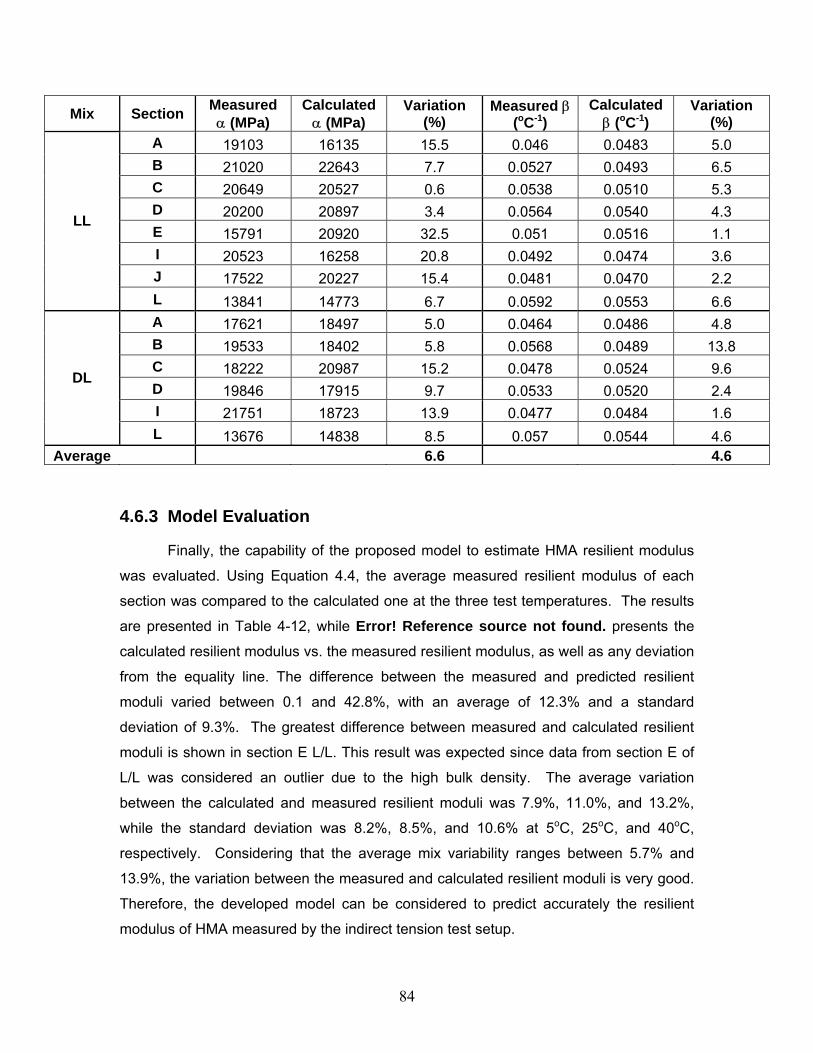
sections is presented in Table 4-10. The different values of α and β suggest that,
although temperature is a major parameter affecting the HMA resilient modulus, other
parameters could also play a role affecting the resilient modulus of HMA. These
identified parameters can be mix properties, mainly bulk density, air voids, asphalt
binder content, voids in mineral aggregates, voids filled with asphalt, G*/sinδ, and fine to
asphalt ratio.
y = 17621e-0.0464x
R2 = 0.967
0
4000
8000
12000
16000
20000
0 10 20 30 40 50
Temperature (°C)
Res
ilien
t Mod
ulus
(MP
a)
Figure 4-5 Resilient Modulus Variation with Temperature (Specimen A1-4in D/L)
80
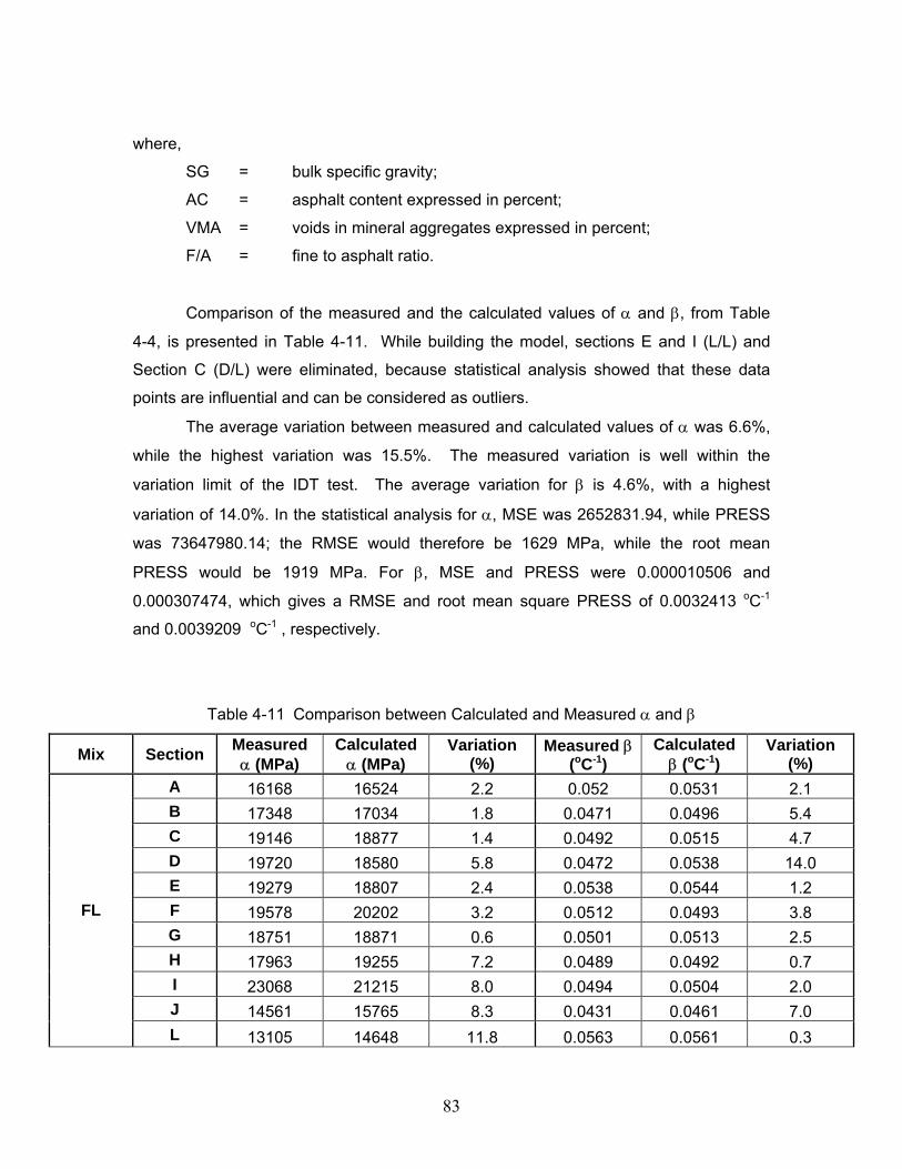
Table 4-9 Values of α and β
α (MPa) F/F F/L L/L D/L D/L-0.03 Sectio
n a* a* b* a* b* a* b* a*
A 11805 16168 12533 19103 12532 17621 10740 14978 B 11327 17348 10201 21020 15624 19533 10201 15603 C 11100 19146 11118 20649 11148 18222 11118 16212 D 13476 19720 16578 20200 11274 19846 11273 17118 E 19279 13089 15791 13575 F 19578 13200 G
NA 18751 14663
H 9119 17963 13499 Same as E Same as B Same as B
I 16146 23068 16872 20523 13441 21751 12653 15443 J 14561 12884 17522 12169 Same as B Same as B L NA 13105 10556 13841 7834 13676 6810 11511
a* 100-mm diameter specimens with 63-mm thickness
b* 150-mm diameter specimens with 75-mm thickness β (oC-1)
A 0.0458 0.052 0.0629 0.046 0.0472 0.0464 0.0541 0.035 B 0.046 0.0471 0.0593 0.0527 0.0517 0.0568 0.0593 0.0401 C 0.0566 0.0492 0.0541 0.0538 0.0561 0.0478 0.0541 0.0348 D 0.0675 0.0472 0.0669 0.0564 0.0637 0.0533 0.0545 0.04 E 0.0538 0.0534 0.051 0.055 F 0.0512 0.0535 G
NA 0.0501 0.0535
H 0.0475 0.0489 0.059 Same as E Same as B Same as B
I 0.0486 0.0494 0.0544 0.0492 0.0551 0.0477 0.0538 0.0272 J 0.0431 0.05 0.0481 0.0498 Same as B Same as B L NA 0.0563 0.0598 0.0592 0.0708 0.057 0.0537 0.0365
81
Table 4-10 R2 Values for the Different Mixes
R2 F/F F/L L/L D/L D/L-0.03 Sectio
n a* a* b* a* b* a* b* a* A 0.81 0.99 0.85 0.98 0.96 0.97 0.98 0.83 B 0.95 0.96 0.98 0.95 0.91 0.95 0.98 0.89 C 0.95 0.93 0.95 0.94 0.94 0.96 0.95 0.82 D 0.99 0.95 0.92 0.94 0.99 0.93 0.97 0.86 E 0.93 0.98 0.92 0.91 F 0.92 0.98 G
NA 0.97 0.97
H 0.43 0.94 0.97 Same as E Same as B Same as B
I 0.98 0.92 0.95 0.94 0.92 0.91 0.92 0.79 J 0.98 0.97 0.86 0.98 Same as B Same as B L NA 0.96 0.98 0.96 0.97 0.94 0.95 0.77
The effect of each mix property on the calculated resilient modulus was
investigated. The procedure for determining the influence and importance of each
parameter includes identifying a trend in resilient modulus variation as a function of the
parameter being considered, analyzing the correlation between the resilient modulus
and each individual parameter, as well as the correlations between the considered
parameters. Five mix parameters were identified as affecting the parameters α and β
and therefore the resilient modulus. The parameters were considered in the
development of the model: bulk specific gravity (SG), air void (AV) content, asphalt
content (AC), voids in mineral aggregates (VMA), and fine to asphalt ratio (F/A), with
bulk specific gravity the most influential parameter on α and asphalt content the most
prominent for parameter β. The next step was to identify highly influential data points
and outliers. During the model building process, three data points were identified as
outliers; therefore, they were excluded from the model building process.
4.6.2 Model Development
The proposed model (Equation 4.1) includes two coefficients that depend on the
mix properties. Coefficient α represents the resilient modulus at 0°C, while coefficient β
represents the sensitivity of the resilient modulus to temperature changes. Using
Equation 4.1, the coefficients α and β were determined for each section. One dilemma
in developing a model arises from uncertainty about which terms to include in the model.
Since five parameters had to be investigated, all possible regressions (25=32) were
82
considered. The final model selected is based on a goodness of fit and a goodness of
prediction criteria.
To validate a certain model, data is usually split into two sets—one set for model
fitting and another set to validate the prediction capabilities of the developed model.
Data splitting requires extensive gathering of data. An alternative to this process
involves calculating the PRESS statistic, which is a measure of a model’s prediction
capabilities, which can be used as a form of validation in the spirit of data splitting. The
PRESS statistic is computed as the sum of squares of the PRESS residuals. The
procedure involves setting aside the first observation from the data set and using the
remaining n-1 observations to estimate the coefficients for a particular candidate model.
The first observation is then replaced and the second observation withheld with
coefficients estimated again. Each observation is removed one at a time, and thus the
candidate model is fitted n times. The deleted response is estimated each time,
resulting in n prediction errors. The model that is finally adopted is fit using the entire
data set, making use of all available information. The model with the lower PRESS
statistic is the one that performs the best for prediction.
Another prediction parameter, the Cp statistic, was also considered during model
selection. The Cp statistic is a compromise between model underfitting and model
overfitting. The model with the lower Cp presents the best compromise between
overfitting and underfitting. The models were also evaluated for fitting ability in the form
of RMSE and the R-squared. In terms of fitting, the model with the higher R-square and
lower MSE is the best model. It should be noted that different models might have
optimum PRESS statistic, Cp, R-square, or MSE. In the end, the best overall model, a
compromise between fitting and predicting capabilities, was selected.
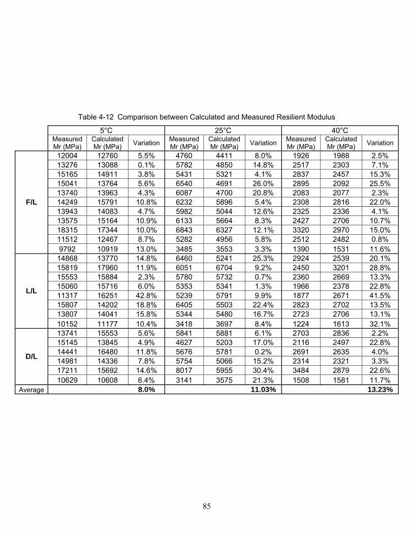
The data used for model development was obtained from 100 mm F/L, L/L, and
D/L specimens. The values of α and β, as well as the R-square (obtained by fitting
equation 4.1 to the data of the measured resilient modulus) is presented in Table 4.6.
Alpha (α) was found to be related to the bulk density, the asphalt content, as well
as to the fine-to-asphalt ratio, while β was found to be related to the bulk density, the
natural log of asphalt content, and the voids in mineral aggregates. The relationships for
α and β are presented in equations 4.2 and 4.3, respectively.
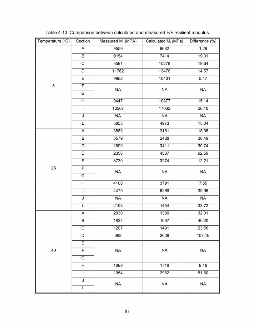
However, such a high average variation is partly due to the variations that occur
in section D at 25oC and 40oC. Quite unexpectedly, the resilient modulus measurements
for section D at 25oC and 40oC were very low, which is probably due to the specimens
being damaged; therefore, these measurements should be considered non-reliable and
should be excluded from the analysis. Doing so would give a maximum variation of
51.6% (section I at 40oC). The average variation would then be 22.3%, with a standard
deviation of 13.1%. The average variation between the model-calculated and measured
resilient moduli is higher than the average mix variability in the resilient modulus test:
10.3%, 8.9%, and 4.3% at 5oC, 25oC, and 40oC, respectively. However, test results of
F/F specimens are based on limited number of data as a result of the limited number of
field cores, as well as the inability to test some specimens at 25 and/or 40oC. In
conclusion, the difference in the measured resilient moduli between F/L and F/F
specimens is partly due to the difference in the volumetric properties, mainly the bulk
density. However, the difference in bulk density does not fully explain this difference,
which confirms the existence of a compaction shift factor between field cores and
laboratory prepared specimens.
4.7 Conclusion
Resilient modulus values were successfully measured using the IDT setup. The
mix variability was determined and it was found that the repeatability of the IDT test is
high. Shift factors for compaction, and load duration were developed. Field compaction
resulted in field cores having lower bulk density and higher air voids than F/L specimens,
however, this fact did not entirely explain the difference in the measured resilient
modulus. The data analysis method used to calculate the measured resilient modulus
(Roque and Buttlar, 1992) was developed to take into account the specimen size effect
by introducing correction factors that are function of the specimen diameter to thickness
ratio. The method is applicable at low temperature, however as the testing temperature
is increased elastic analysis lead to discrepancies between the 100- and 150-mm
specimen diameter resilient modulus values. The load duration was found to have an
effect on the measured resilient modulus. The effect of load duration increased with
increasing temperature. However an interesting finding was the fact that the resilient
modulus measured at 0.1 sec load duration was higher than the one measured at 0.03
sec load duration at 5oC, which might be related to the method the IDT test is performed.
89
Finally a model predicting resilient modulus values from volumetric properties was
successfully developed. The resilient modulus values predicted by the model fell well
within the range of the test variability.
90
Chapter 5 Findings, Conclusions, and Recommendations
5.1 Summary
Accurate determination of the material properties is essential for pavement design,
maintenance, and rehabilitation. Laboratory testing has the advantage of determining
the material properties before the pavement is constructed. Upon completion of the
construction, the as built material properties can be determined using FWD testing or by
laboratory testing of field cores. The main objective of this research was to develop shift
factors between field cores and laboratory prepared specimens. Determining these shift
factors allows pavement engineers to determine whether the difference between the
laboratory prepared specimens or field cores resilient modulus is due to compaction or
construction. Moreover, such a shift factor is important during the design stage when
resilient modulus values can be obtained from specimens prepared in the laboratory.
Laboratory specimens were prepared using HMA either mixed at the plant during
construction or mixed in the laboratory. Also the effect of load pulse duration on the
resilient modulus was investigated. The load pulses investigated are 0.1s (as
recommended by ASTM D4123) and 0.03s (based on a study on the stress pulse width
and truck loading by Loulizi et al., 2002). The tasks that were undertaken in this
research can be summarized as follows:
1. Specimen preparation; the specimens were divided into F/F, F/L, L/L, D/L, and
D/L tested at 0.03s load pulse duration.
2. Determine the load to be used for resilient modulus testing at each of the testing
temperatures for the different mixes. The selected load had to meet the criterion
of limiting the strain between 150 and 500 microstrains.
3. Determine the variability in the IDT test. The variability was divided into two
parts: (1) variability between the two faces of the IDT specimen, and (2)
variability between the specimens of a given mix.
4. Determine the compaction shift factor at each of the testing temperatures
between F/F, and F/L specimens.
5. Determine the specimen size shift factor between 100- and 150-mm diameter
specimens for F/L/, L/L, and D/L specimens.
91
6. Determine the load pulse duration shift factor between 0.1s and 0.03s load
pulses; this was performed on D/L specimens.
7. Develop a model to correlate the resilient modulus to the temperature and the
volumetric properties of the HMA using F/L, L/L, and D/L specimens. This model
was then used to calculate the resilient modulus of F/F specimens and compare
the results to the measured resilient modulus of F/F specimens.
5.2 Findings
Various findings were encountered during this research. These findings can be
summarized as follows:
1. In the tested load range, the resilient modulus was found to be independent of
the applied load at 5oC and 25oC. This could not be verified at 40oC due to the
limited range of tested loads. The reason for the independence of the resilient
modulus to the load intensity is thought to be due to the fact that the tested load
range is relatively small compared to the indirect tensile strength of the
specimens.
2. Damage to an indirect tension specimen is avoided when the strain is limited
between 150 and 500 microstrain.
3. The average specimen variability ranged between 6.7% and 35.5%, while the
average mix variability ranged between 5.7% and 13.9%. This indicates that the
repeatability of the indirect tension test for resilient modulus calculation is
acceptable. Moreover it was found that repeatability is better achieved for
specimens produced in the laboratory than for specimens taken from the field.
4. The study showed that there is a compaction shift factor between field cores and
laboratory compacted specimens. The shift factor ranged from 1 to 3 with
laboratory compacted samples having the higher resilient modulus. An average
shift factor ranging between 1.45 and 1.5 seems to represent most mixes at all
tested temperatures. The existence of a shift factor is reinforced by the fact that
different air void content and specific gravity were measured for F/F and F/L
samples.
5. The data analysis procedure used in calculating the resilient modulus accounted
for the specimen size effect at 5oC. At 5oC the behavior of HMA is elastic and
therefore correcting for the specimen size using an elastic analysis resulted in a
92
consistent resilient modulus measured for 100- and 150-mm diameter.
However, at 25 and 40oC, viscous flow in the specimen resulted in different
resilient modulus from 100- and 150-mm diameter specimens, with the former
resulting in a higher calculated resilient modulus. The specimen size shift factor
increased as the test temperature increased. The average specimen size shift
factor was 1.25, and 1.30 at 25, and 40oC, respectively.
6. Analysis of the variability in resilient modulus results showed no difference
between 100- and 150-mm diameter specimens which means that 100-mm
diameter specimens as accurate as 150-mm diameter specimens in determining
the resilient modulus however, the measured values are not the same.
7. The average load duration shift factor varied with temperature, with average load
duration shift factors of 0.83, 1.31 and 1.39 at 5oC, 25oC, and 40oC, respectively.
These shift factors represent the ratio of the measured resilient modulus at 0.03
sec to the measured resilient modulus at 0.1 sec load duration. An interesting
result is the load duration shift factor at 5oC which is smaller than one. The
explanation for this fact is that the total accumulated strain using a load duration
of 0.1 sec is higher than the one accumulated using a load duration of 0.03 sec.
This might lead to lower resilient moduli being measured at a 0.03 sec loading
duration. This factor was verified by measuring the resilient modulus at 0.03 sec
and 0.1 sec on the same samples which also produced the same shift factor.
8. In characterizing the resilient modulus as a function of temperature, two
parameters α and β were identified. α is related to the resilient modulus at 0oC
while β represents the mix sensitivity to temperature. These two parameters were
related to the mix volumetric properties. α was found to be affected by the mix
specific gravity, the asphalt content, and the fine to asphalt ratio; while β was
found to be affected by the asphalt content, the specific gravity, and the voids in
mineral aggregates. A model was developed to predict the resilient modulus from
the mix volumetric properties. The average variation between the model
calculated and measured resilient modulus was 7.95%, 11.03%, and 13.23% at
5oC, 25oC, and 40oC, respectively, which is lower than the average mix variation
in the indirect tension test for the resilient modulus.
93
5.3 Conclusions
The resilient moduli of the different HMA placed at the Virginia Smart Road were
measured in the laboratory using the IDT setup. The variability in the result was
determined and shift factors were developed to account for the effect of compaction,
specimen size, and load pulse duration. Finally, a model that relates the resilient
modulus to the volumetric properties of the mix was developed. Based on this research,
the following conclusions could be drawn:
1. The testing results suggest that as long as the applied load is under 20% of the
load to cause failure in the specimen, the resilient modulus of HMA will be
independent of the applied load; this is based on results of tests at 25oC.
2. There is a difference between field compaction and laboratory gyratory
compaction. The difference results in different resilient moduli between field
cores and laboratory produced specimens and cannot fully be explained by the
fact that the percent air voids and bulk specific gravity are different for the two
sets of specimens.
3. The load duration affects the resilient modulus results. Therefore, resilient
modulus results obtained at loading durations similar to the ones experienced in
the field should be used for HMA characterization.
4. There is a strong correlation between the resilient modulus of HMA and its
volumetric properties. These volumetric properties are the bulk specific gravity,
the asphalt content, the fine to asphalt ratio, and the voids in mineral aggregate.
A model was developed to predict the HMA resilient modulus from its volumetric
properties
5.4 Recommendations
Based on the research’s results the following recommendations for testing and future
research can be made:
1. It is clear that the load duration has an effect on the measured resilient modulus
therefore, it is suggested that a load pulse duration of 0.03 sec be used since it is
more representative of the actual traffic loading.
2. The range of the applied load in this research was small compared to the indirect
tensile strength of the HMA. In this range, the load had no effect on the
94
measured resilient modulus. To investigate the effect of load intensity on the
measured resilient modulus using Roque and Buttlar’s data analysis, the Load
intensity range must be increased. Roque and Buttlar showed that a strain of
2000 microstrain may be needed to induce damage to the samples; therefore,
the loading can be safely increased to investigate its effect on the resilient
modulus.
3. The shift factor between field and laboratory compaction might be partly due to
the difference in the sample thickness between F/F and F/L samples. To fully
account for the effect of compaction, specimens of the same thickness and same
diameter to thickness ratio should be tested.
4. it appears that the viscous flow of HMA in the resilient modulus testing is affected
by the thickness to diameter ratio. To quantify this effect, it is suggested that a
wider range of specimen diameters and thicknesses be investigated.
5. To quantify the effect of HMA volumetric properties on its resilient modulus for
different mixes, it is suggested that a wider range of volumetric and binder
properties be used to fine-tune and calibrate the developed model for other HMA.
95
References
Almudaiheem, J., and Al-Sugair, F., “Effect of Loading Magnitude on Measured Resilient Modulus of Asphalt Concrete Mixes.” Transportation Research Record, No.1317, Transportation Research Board, Washington, DC, pp.139-144, 1991. Baladi, Gilbert Y. Harichandran, Ronald S. Lyles, Richard W. “New relationships between structural properties and asphalt mix parameters.” Transportation Research Record n 1171 1988 p 168-177 Blakey, F.A., and Beresford, F.D., “Tensile Strain in Concrete” II. C.S.I.R.O. Div. Build. Res. Rep. No. C2. 2-2, 15, 1955. Brown, E.R., and Foo, Kee Y., “Evaluation of Variability in Resilient Modulus Test Results (ASTM D 4123)”, ASTM Journal of Testing & Evaluation, Vol. 19 No 1, p 1-13, 1991. Cragg R. Pell PS. “Dynamic stiffness of bituminous road materials” Proceding of the Association of Asphalt Paving Technologists, Tech Session, Oklahoma City, Okla,. v 40 Feb 15-17 1971 p 126-47 Gemayel, Chaouki A. Mamlouk, Michael S. Characterization of hot-mixed open-graded asphalt mixtures. Transportation Research Record n 1171 1988 p 184-192 Heinicke, John J. Vinson, Ted S. “EFFECT OF TEST CONDITION PARAMETERS ON IRMR”. Journal of Transportation Engineering. v 114 n 2 Mar 1988 p 153-172 Hondros, G., “The Evaluation of Poisson’s Ratio and the Modulus of Materials of a Low Tensile Resistance by the Brazilian (Indirect Tensile) Test with Particular Reference to Concrete”, Australian Journal of Applied Science, Vol. 10, No. 3, p. 243-268, 1959. Howeedy, M Fayek, Herrin, Moreland. BEHAVIOR OF COLD MIXES UNDER REPEATED COMPRESSIVE LOADS. Highw Res Rec. n 404, 1972 p 57-70 Kim, Y.R., Shah, K.A, and Khosla, N.P, “Influence of Test Parameters in SHRP P07 Procedure on Resilient Moduli of Asphalt Concrete Field Cores”, Transportation Research Record 1353, p.82-89, 1992. Lim, C.T., Tan, S.A., Fwa, T.F., “Specimen Size Effect on The Diametrical Mechanical Testing of Asphalt Mixes”, Journal of Testing and Evaluation, JTEVA, Vol. 23, No. 6, pp. 436-441, 1995.
96
Loulizi, A., Al-Qadi, I.L., Lahour, S., and Freeman, T.E., “Measurement of Vertical Compressive Stress Pulse in Flexible Pavements and Its Representation for Dynamic Loading”, Transportation Research Board, Paper No.02-2376, 2002. Myers, R.H., “Classical and Modern Regression with Applications”, second edition Roque, R., and Ruth, B.E., “Materials Characterization and Response of Flexible Pavements at Low Temperatures.” Proceedings of the Association of Asphalt Paving Technoligists, Vol. 56, pp. 130-167, 1987. Roque, R., and Buttlar, W.G., “Development of a Measurement and Analysis Method to accurately Determine Asphalt concrete Properties Using the Indirect Tensile Mode”, Proc., Association of Asphalt Paving Technologists, Vol. 61, 1992. Schmidt, R J. “PRACTICAL METHOD FOR MEASURING THE RESILIENT MODULUS OF ASPHALT-TREATED MIXES.” Highway Research Record n 404, 1972 p 22-29 15. Von Quintus, Harold L. Harrigan, Edward. Lytton, Robert L. How SHRP reliably predicts pavement performance Pacific Rim TransTech Conference. Publ by ASCE, New York, NY, USA. 1993. p 298-307 Wright, P.J.F., “Comments on an indirect tensile test for concrete” Mag. Conc. Res. 20: 87-96, 1955.
97
Appendix A
Mixture Designs and Gradations
98
%#78 Quartzite Salem Stone Co., Sylvatus, VA 15#8 Quartzite Salem Stone Co., Sylvatus, VA 30#9 Quartzite Salem Stone Co., Sylvatus, VA 10
#10 Limestone Sisson and Ryan Quarry, Shawsville, VA 20Sand Castle Sand Co., New Castle VA 10
Fine RAP Adams Construction Co., Blacksburg, VA 15%
PG 70-22 Associated Asphalt, Inc., Roanoke, VA 5.6
%#78 Quartzite Salem Stone Co., Sylvatus, VA 5#8 Quartzite Salem Stone Co., Sylvatus, VA 30#9 Quartzite Salem Stone Co., Sylvatus, VA 20
#10 Limestone Sisson and Ryan Quarry, Shawsville, VA 20Sand Castle Sand Co., New Castle VA 10
Fine RAP 15%
PG 70-22 Associated Asphalt, Inc., Roanoke, VA 5.9Binder
Binder
Design / LabAggregate
Lab / LabAggregate
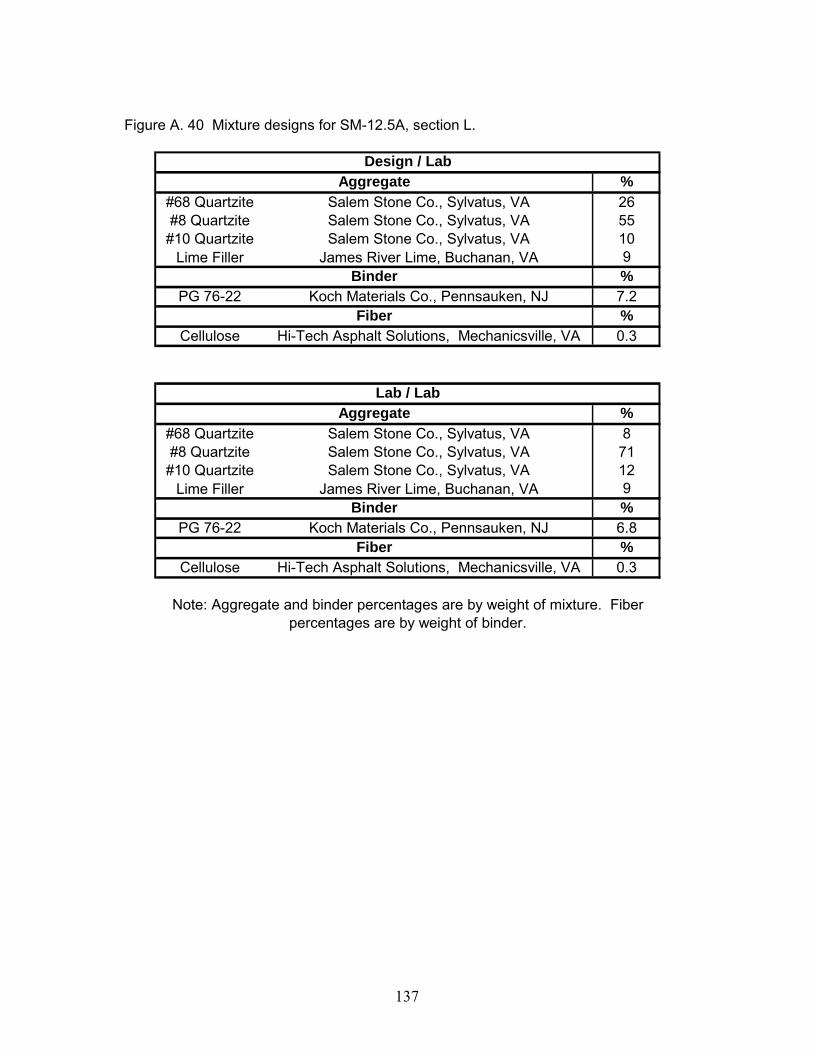
Figure A.1 Mixture designs for SM12.5D, section A.
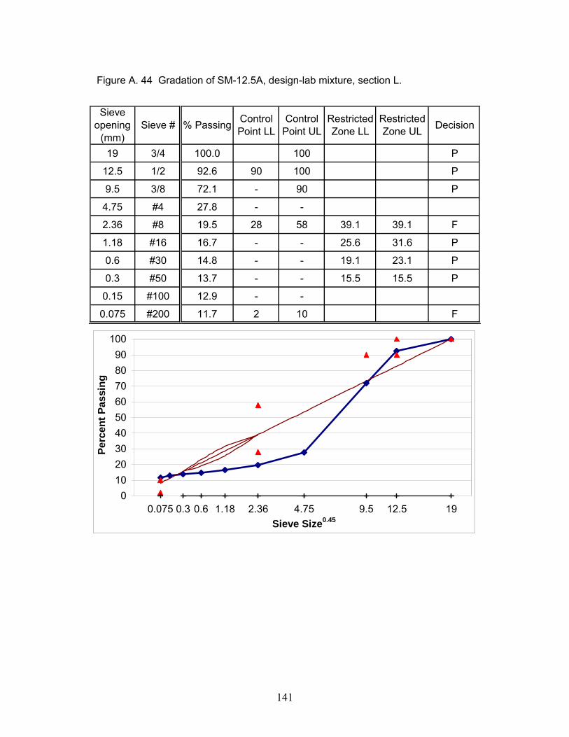
99
Figure A. 2 Gradation of SM-12.5D, field-field mixture, section A.
Sieve opening
(mm)Sieve # % Passing Control
Point LLControl
Point ULRestricted Zone LL
Restricted Zone UL Decision
19 3/4 100.0 - 100 - - -
12.5 1/2 99.6 90 100 - - P
9.5 3/8 98.5 - 90 - - F
4.75 #4 84.2 - - - - -
2.36 #8 47.7 28 58 39.1 39.1 P
1.18 #16 37.3 - - 25.6 31.6 P
0.6 #30 27.0 - - 19.1 23.1 P
0.3 #50 14.7 - - 15.5 15.5 P
0.15 #100 10.2 - - - - -
0.075 #200 5.6 2 10 - - P
1912.59.54.752.361.180.60.30.0750
102030405060708090
100
Sieve Size0.45
Perc
ent P
assi
ng
100
Figure A. 3 Gradation of SM-12.5D, field-lab mixture, section A.
Sieve opening
(mm)Sieve # % Passing Control
Point LLControl
Point ULRestricted Zone LL
Restricted Zone UL Decision
19 3/4 100.0 - 100 - - P
12.5 1/2 99.6 90 100 - - P
9.5 3/8 98.5 - 90 - - F
4.75 #4 84.2 - - - - -
2.36 #8 47.7 28 58 39.1 39.1 P
1.18 #16 37.3 - - 25.6 31.6 P
0.6 #30 27.0 - - 19.1 23.1 P
0.3 #50 14.7 - - 15.5 15.5 P
0.15 #100 10.2 - - - - -
0.075 #200 5.6 2 10 - - P
1912.59.54.752.361.180.60.30.0750
102030405060708090
100
Sieve Size0.45
Perc
ent P
assi
ng
101
Figure A. 4 Gradation of SM-12.5D, lab-lab mixture, section A.
Sieve opening
(mm)Sieve # % Passing Control
Point LLControl
Point ULRestricted Zone LL
Restricted Zone UL Decision
19 3/4 100.0 100 P
12.5 1/2 99.5 90 100 P
9.5 3/8 98.9 - 90 F
4.75 #4 91.3 - -
2.36 #8 58.3 28 58 39.1 39.1 F
1.18 #16 38.8 - - 25.6 31.6 P
0.6 #30 28.7 - - 19.1 23.1 P
0.3 #50 20.1 - - 15.5 15.5 P
0.15 #100 15.6 - -
0.075 #200 12.3 2 10 F
1912.59.54.752.361.180.60.30.0750
102030405060708090
100
Sieve Size0.45
Perc
ent P
assi
ng
102
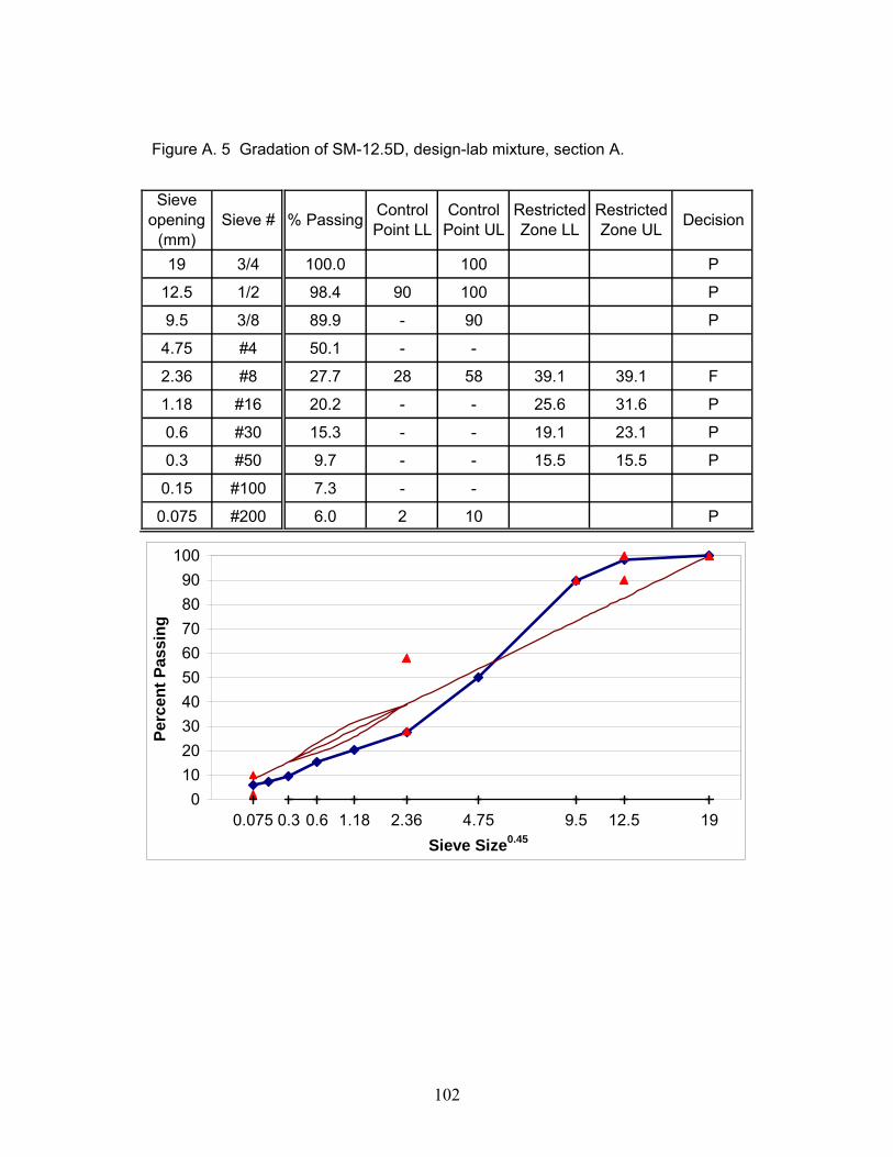
Figure A. 5 Gradation of SM-12.5D, design-lab mixture, section A.
Sieve opening
(mm)Sieve # % Passing Control
Point LLControl
Point ULRestricted Zone LL
Restricted Zone UL Decision
19 3/4 100.0 100 P
12.5 1/2 98.4 90 100 P
9.5 3/8 89.9 - 90 P
4.75 #4 50.1 - -
2.36 #8 27.7 28 58 39.1 39.1 F
1.18 #16 20.2 - - 25.6 31.6 P
0.6 #30 15.3 - - 19.1 23.1 P
0.3 #50 9.7 - - 15.5 15.5 P
0.15 #100 7.3 - -
0.075 #200 6.0 2 10 P
1912.59.54.752.361.180.60.30.0750
102030405060708090
100
Sieve Size0.45
Perc
ent P
assi
ng
103
%#8 Quartzite Salem Stone Co., Sylvatus, VA 60
#10 Limestone ACCO Stone Co., Blacksburg, VA 20Concrete Sand Wythe Stone Co., Wytheville, VA 10
Fine RAP Adams Construction Co., Blacksburg, VA 10%
PG 70-22 Associated Asphalt, Inc., Roanoke, VA 5.6
%#8 Quartzite Salem Stone Co., Sylvatus, VA 36
#10 Limestone ACCO Stone Co., Blacksburg, VA 20Concrete Sand Wythe Stone Co., Wytheville, VA 10#10 Quartzite Salem Stone Co., Sylvatus, VA 23
ite passing #200 Salem Stone Co., Sylvatus, VA 1Fine RAP Adams Construction Co., Blacksburg, VA 10
%PG 70-22 Associated Asphalt, Inc., Roanoke, VA 4.7
Design / Lab
Lab / Lab
Binder
Binder
Aggregate
Aggregate
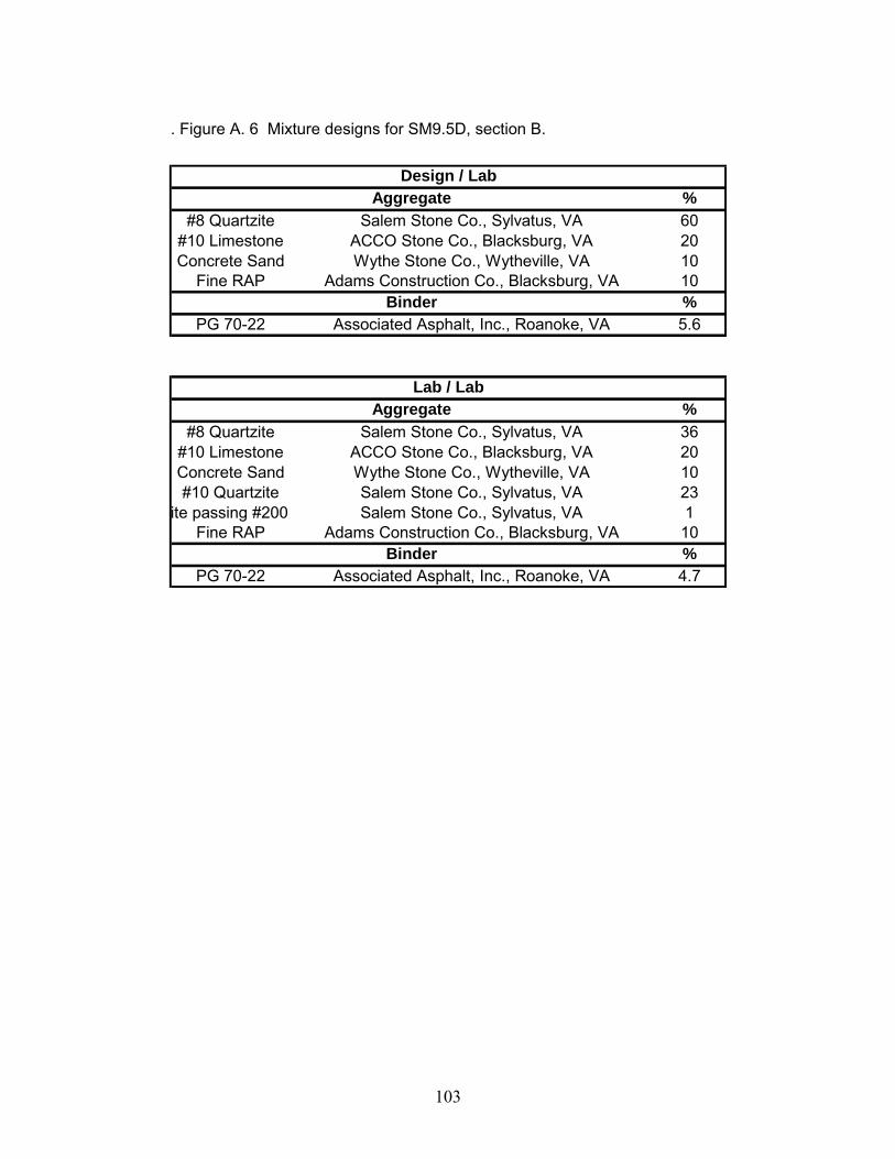
. Figure A. 6 Mixture designs for SM9.5D, section B.
104
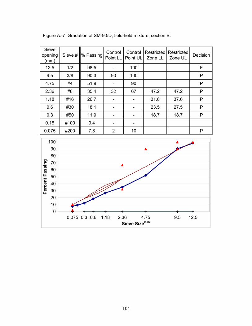
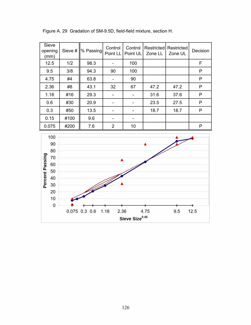
Figure A. 7 Gradation of SM-9.5D, field-field mixture, section B.
Sieve opening
(mm)Sieve # % Passing Control
Point LLControl
Point ULRestricted Zone LL
Restricted Zone UL Decision
12.5 1/2 98.5 - 100 F
9.5 3/8 90.3 90 100 P
4.75 #4 51.9 - 90 P
2.36 #8 35.4 32 67 47.2 47.2 P
1.18 #16 26.7 - - 31.6 37.6 P
0.6 #30 18.1 - - 23.5 27.5 P
0.3 #50 11.9 - - 18.7 18.7 P
0.15 #100 9.4 - -
0.075 #200 7.8 2 10 P
12.59.54.752.361.180.60.30.0750
102030405060708090
100
Sieve Size0.45
Perc
ent P
assi
ng
105
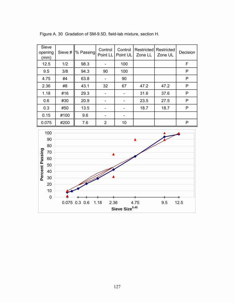
Figure A. 8 Gradation of SM-9.5D, field-lab mixture, section B.
Sieve opening
(mm)Sieve # % Passing Control
Point LLControl
Point ULRestricted Zone LL
Restricted Zone UL Decision
12.5 1/2 98.5 - 100 F
9.5 3/8 90.3 90 100 P
4.75 #4 51.9 - 90 P
2.36 #8 35.4 32 67 47.2 47.2 P
1.18 #16 26.7 - - 31.6 37.6 P
0.6 #30 18.1 - - 23.5 27.5 P
0.3 #50 11.9 - - 18.7 18.7 P
0.15 #100 9.4 - -
0.075 #200 7.8 2 10 P
12.59.54.752.361.180.60.30.0750
102030405060708090
100
Sieve Size0.45
Perc
ent P
assi
ng
106
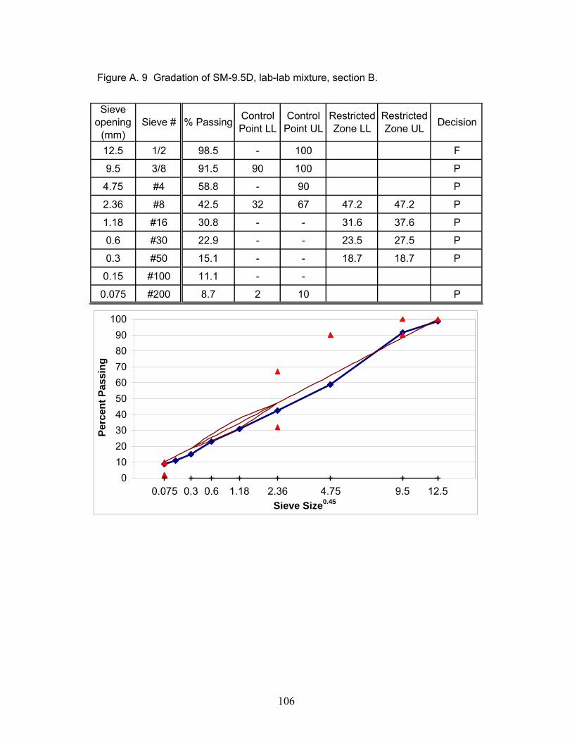
Figure A. 9 Gradation of SM-9.5D, lab-lab mixture, section B.
Sieve opening
(mm)Sieve # % Passing Control
Point LLControl
Point ULRestricted Zone LL
Restricted Zone UL Decision
12.5 1/2 98.5 - 100 F
9.5 3/8 91.5 90 100 P
4.75 #4 58.8 - 90 P
2.36 #8 42.5 32 67 47.2 47.2 P
1.18 #16 30.8 - - 31.6 37.6 P
0.6 #30 22.9 - - 23.5 27.5 P
0.3 #50 15.1 - - 18.7 18.7 P
0.15 #100 11.1 - -
0.075 #200 8.7 2 10 P
12.59.54.752.361.180.60.30.0750
102030405060708090
100
Sieve Size0.45
Perc
ent P
assi
ng
107
Figure A. 10 Gradation of SM-9.5D, design-lab mixture, section B.
Sieve opening
(mm)Sieve # % Passing Control
Point LLControl
Point ULRestricted Zone LL
Restricted Zone UL Decision
12.5 1/2 99.7 - 100 F
9.5 3/8 86.1 90 100 F
4.75 #4 33.7 - 90 P
2.36 #8 22.9 32 67 47.2 47.2 F
1.18 #16 18.2 - - 31.6 37.6 P
0.6 #30 14.0 - - 23.5 27.5 P
0.3 #50 8.8 - - 18.7 18.7 P
0.15 #100 6.6 - -
0.075 #200 5.5 2 10 P
12.59.54.752.361.180.60.30.0750
102030405060708090
100
Sieve Size0.45
Perc
ent P
assi
ng
108
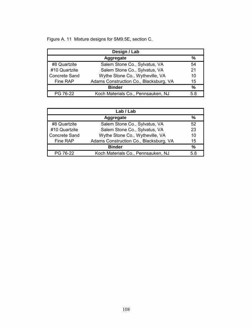
%#8 Quartzite Salem Stone Co., Sylvatus, VA 54
#10 Quartzite Salem Stone Co., Sylvatus, VA 21Concrete Sand Wythe Stone Co., Wytheville, VA 10
Fine RAP Adams Construction Co., Blacksburg, VA 15%
PG 76-22 Koch Materials Co., Pennsauken, NJ 5.8
%#8 Quartzite Salem Stone Co., Sylvatus, VA 52
#10 Quartzite Salem Stone Co., Sylvatus, VA 23Concrete Sand Wythe Stone Co., Wytheville, VA 10
Fine RAP Adams Construction Co., Blacksburg, VA 15%
PG 76-22 Koch Materials Co., Pennsauken, NJ 5.8
Design / Lab
Lab / Lab
Binder
Binder
Aggregate
Aggregate
Figure A. 11 Mixture designs for SM9.5E, section C.
109
Figure A. 12 Gradation of SM-9.5E, field-field mixture, section C.
Sieve opening
(mm)Sieve # % Passing Control
Point LLControl
Point ULRestricted Zone LL
Restricted Zone UL Decision
12.5 1/2 99.4 - 100 F
9.5 3/8 95.0 90 100 P
4.75 #4 61.7 - 90 P
2.36 #8 40.3 32 67 47.2 47.2 P
1.18 #16 29.2 - - 31.6 37.6 P
0.6 #30 22.6 - - 23.5 27.5 P
0.3 #50 15.3 - - 18.7 18.7 P
0.15 #100 10.7 - -
0.075 #200 8.2 2 10 P
12.59.54.752.361.180.60.30.0750
102030405060708090
100
Sieve Size0.45
Perc
ent P
assi
ng
110
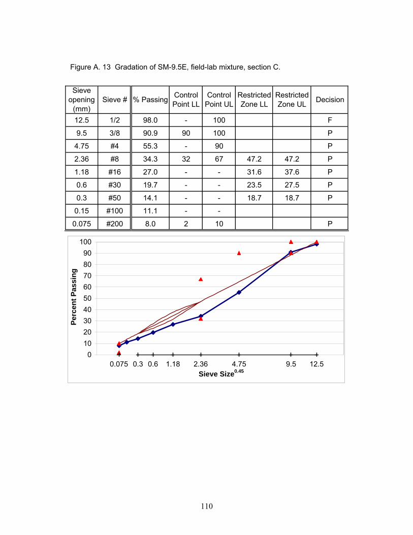
Figure A. 13 Gradation of SM-9.5E, field-lab mixture, section C.
Sieve opening
(mm)Sieve # % Passing Control
Point LLControl
Point ULRestricted Zone LL
Restricted Zone UL Decision
12.5 1/2 98.0 - 100 F
9.5 3/8 90.9 90 100 P
4.75 #4 55.3 - 90 P
2.36 #8 34.3 32 67 47.2 47.2 P
1.18 #16 27.0 - - 31.6 37.6 P
0.6 #30 19.7 - - 23.5 27.5 P
0.3 #50 14.1 - - 18.7 18.7 P
0.15 #100 11.1 - -
0.075 #200 8.0 2 10 P
12.59.54.752.361.180.60.30.0750
102030405060708090
100
Sieve Size0.45
Perc
ent P
assi
ng
111
Figure A. 14 Gradation of SM-9.5E, lab-lab mixture, section C.
Sieve opening
(mm)Sieve # % Passing Control
Point LLControl
Point ULRestricted Zone LL
Restricted Zone UL Decision
12.5 1/2 99.7 - 100 F
9.5 3/8 90.2 90 100 P
4.75 #4 44.6 - 90 P
2.36 #8 35.2 32 67 47.2 47.2 P
1.18 #16 27.3 - - 31.6 37.6 P
0.6 #30 21.0 - - 23.5 27.5 P
0.3 #50 13.8 - - 18.7 18.7 P
0.15 #100 10.1 - -
0.075 #200 7.6 2 10 P
12.59.54.752.361.180.60.30.0750
102030405060708090
100
Sieve Size0.45
Perc
ent P
assi
ng
112
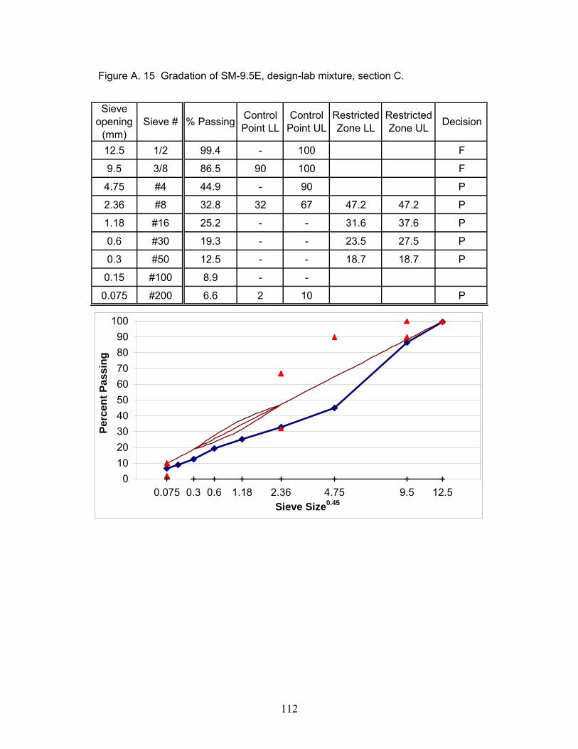
Figure A. 15 Gradation of SM-9.5E, design-lab mixture, section C.
Sieve opening
(mm)Sieve # % Passing Control
Point LLControl
Point ULRestricted Zone LL
Restricted Zone UL Decision
12.5 1/2 99.4 - 100 F
9.5 3/8 86.5 90 100 F
4.75 #4 44.9 - 90 P
2.36 #8 32.8 32 67 47.2 47.2 P
1.18 #16 25.2 - - 31.6 37.6 P
0.6 #30 19.3 - - 23.5 27.5 P
0.3 #50 12.5 - - 18.7 18.7 P
0.15 #100 8.9 - -
0.075 #200 6.6 2 10 P
12.59.54.752.361.180.60.30.0750
102030405060708090
100
Sieve Size0.45
Perc
ent P
assi
ng
113
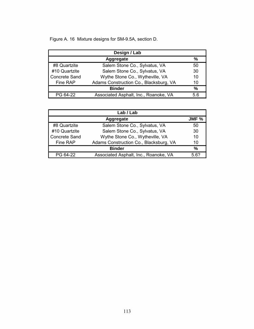
%#8 Quartzite Salem Stone Co., Sylvatus, VA 50
#10 Quartzite Salem Stone Co., Sylvatus, VA 30Concrete Sand Wythe Stone Co., Wytheville, VA 10
Fine RAP Adams Construction Co., Blacksburg, VA 10%
PG 64-22 Associated Asphalt, Inc., Roanoke, VA 5.6
JMF %#8 Quartzite Salem Stone Co., Sylvatus, VA 50
#10 Quartzite Salem Stone Co., Sylvatus, VA 30Concrete Sand Wythe Stone Co., Wytheville, VA 10
Fine RAP Adams Construction Co., Blacksburg, VA 10%
PG 64-22 Associated Asphalt, Inc., Roanoke, VA 5.6?
Design / Lab
Binder
Binder
Lab / Lab
Aggregate
Aggregate
Figure A. 16 Mixture designs for SM-9.5A, section D.
114
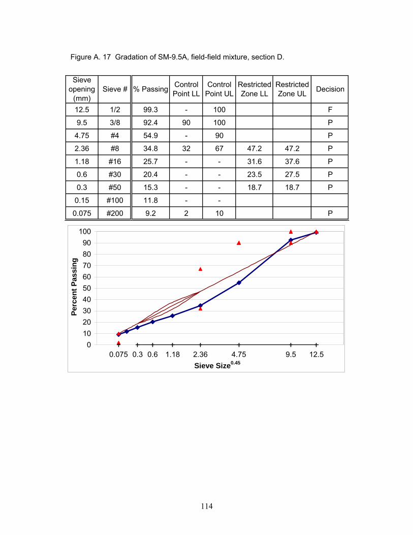
Figure A. 17 Gradation of SM-9.5A, field-field mixture, section D.
Sieve opening
(mm)Sieve # % Passing Control
Point LLControl
Point ULRestricted Zone LL
Restricted Zone UL Decision
12.5 1/2 99.3 - 100 F
9.5 3/8 92.4 90 100 P
4.75 #4 54.9 - 90 P
2.36 #8 34.8 32 67 47.2 47.2 P
1.18 #16 25.7 - - 31.6 37.6 P
0.6 #30 20.4 - - 23.5 27.5 P
0.3 #50 15.3 - - 18.7 18.7 P
0.15 #100 11.8 - -
0.075 #200 9.2 2 10 P
12.59.54.752.361.180.60.30.0750
102030405060708090
100
Sieve Size0.45
Perc
ent P
assi
ng
115
Figure A. 18 Gradation of SM-9.5A, field-lab mixture, section D.
Sieve opening
(mm)Sieve # % Passing Control
Point LLControl
Point ULRestricted Zone LL
Restricted Zone UL Decision
12.5 1/2 99.3 - 100 F
9.5 3/8 92.4 90 100 P
4.75 #4 54.9 - 90 P
2.36 #8 34.8 32 67 47.2 47.2 P
1.18 #16 25.7 - - 31.6 37.6 P
0.6 #30 20.4 - - 23.5 27.5 P
0.3 #50 15.3 - - 18.7 18.7 P
0.15 #100 11.8 - -
0.075 #200 9.2 2 10 P
12.59.54.752.361.180.60.30.0750
102030405060708090
100
Sieve Size0.45
Perc
ent P
assi
ng
116
Figure A.19 Gradation of SM-9.5A, lab-lab mixture, section D.
Sieve opening
(mm)Sieve # % Passing Control
Point LLControl
Point ULRestricted Zone LL
Restricted Zone UL Decision
12.5 1/2 100.0 - 100 P
9.5 3/8 89.3 90 100 F
4.75 #4 50.8 - 90 P
2.36 #8 37.0 32 67 47.2 47.2 P
1.18 #16 27.7 - - 31.6 37.6 P
0.6 #30 20.4 - - 23.5 27.5 P
0.3 #50 12.3 - - 18.7 18.7 P
0.15 #100 8.0 - -
0.075 #200 5.7 2 10 P
12.59.54.752.361.180.60.30.0750
102030405060708090
100
Sieve Size0.45
Perc
ent P
assi
ng
117
Figure A. 20 Gradation of SM-9.5A, design-lab mixture, section D.
Sieve opening
(mm)Sieve # % Passing Control
Point LLControl
Point ULRestricted Zone LL
Restricted Zone UL Decision
12.5 1/2 99.2 - 100 F
9.5 3/8 92.3 90 100 P
4.75 #4 58.3 - 90 P
2.36 #8 41.7 32 67 47.2 47.2 P
1.18 #16 28.7 - - 31.6 37.6 P
0.6 #30 20.3 - - 23.5 27.5 P
0.3 #50 12.4 - - 18.7 18.7 P
0.15 #100 8.6 - -
0.075 #200 6.3 2 10 P
12.59.54.752.361.180.60.30.0750
102030405060708090
100
Sieve Size0.45
Perc
ent P
assi
ng
118
%#8 Quartzite Salem Stone Co., Sylvatus, VA 60
#10 Limestone ACCO Stone Co., Blacksburg, VA 20Concrete Sand Wythe Stone Co., Wytheville, VA 10
Fine RAP Adams Construction Co., Blacksburg, VA 10%
PG 70-22 Associated Asphalt, Inc., Roanoke, VA 5.4
%#8 Quartzite Salem Stone Co., Sylvatus, VA 48
#10 Quartzite Salem Stone Co., Sylvatus, VA 12#10 Limestone ACCO Stone Co., Blacksburg, VA 20Concrete Sand Wythe Stone Co., Wytheville, VA 10
Fine RAP Adams Construction Co., Blacksburg, VA 10%
PG 70-22 Associated Asphalt, Inc., Roanoke, VA 5.8
Lab / Lab
Binder
Binder
Design / LabAggregate
Aggregate
Figure A. 21 Mixture designs for SM9.5D, setions E, F, G, and H.
119
Figure A. 22 Gradation of SM-9.5D, field-field mixture, section E.
Sieve opening
(mm)Sieve # % Passing Control
Point LLControl
Point ULRestricted Zone LL
Restricted Zone UL Decision
12.5 1/2 97.6 - 100 F
9.5 3/8 92.9 90 100 P
4.75 #4 63.3 - 90 P
2.36 #8 42.6 32 67 47.2 47.2 P
1.18 #16 31.5 - - 31.6 37.6 P
0.6 #30 20.5 - - 23.5 27.5 P
0.3 #50 13.3 - - 18.7 18.7 P
0.15 #100 10.4 - -
0.075 #200 7.6 2 10 P
12.59.54.752.361.180.60.30.0750
102030405060708090
100
Sieve Size0.45
Perc
ent P
assi
ng
120
Figure A. 23 Gradation of SM-9.5D, field-lab mixture, section E.
Sieve opening
(mm)Sieve # % Passing Control
Point LLControl
Point ULRestricted Zone LL
Restricted Zone UL Decision
12.5 1/2 97.6 - 100 F
9.5 3/8 92.9 90 100 P
4.75 #4 63.3 - 90 P
2.36 #8 42.6 32 67 47.2 47.2 P
1.18 #16 31.5 - - 31.6 37.6 P
0.6 #30 20.5 - - 23.5 27.5 P
0.3 #50 13.3 - - 18.7 18.7 P
0.15 #100 10.4 - -
0.075 #200 7.6 2 10 P
12.59.54.752.361.180.60.30.0750
102030405060708090
100
Sieve Size0.45
Perc
ent P
assi
ng
121
Figure A. 24 Gradation of SM-9.5D, lab-lab mixture, section E.
Sieve opening
(mm)Sieve # % Passing Control
Point LLControl
Point ULRestricted Zone LL
Restricted Zone UL Decision
12.5 1/2 99.3 - 100 F
9.5 3/8 93.0 90 100 P
4.75 #4 61.4 - 90 P
2.36 #8 42.4 32 67 47.2 47.2 P
1.18 #16 31.0 - - 31.6 37.6 P
0.6 #30 23.0 - - 23.5 27.5 P
0.3 #50 15.2 - - 18.7 18.7 P
0.15 #100 11.1 - -
0.075 #200 8.5 2 10 P
12.59.54.752.361.180.60.30.0750
102030405060708090
100
Sieve Size0.45
Perc
ent P
assi
ng
122
Figure A. 25 Gradation of SM-9.5D, field-field mixture, section F.
Sieve opening
(mm)Sieve # % Passing Control
Point LLControl
Point ULRestricted Zone LL
Restricted Zone UL Decision
12.5 1/2 97.6 - 100 F
9.5 3/8 92.9 90 100 P
4.75 #4 63.3 - 90 P
2.36 #8 42.6 32 67 47.2 47.2 P
1.18 #16 31.5 - - 31.6 37.6 P
0.6 #30 20.5 - - 23.5 27.5 P
0.3 #50 13.3 - - 18.7 18.7 P
0.15 #100 10.4 - -
0.075 #200 7.6 2 10 P
12.59.54.752.361.180.60.30.0750
102030405060708090
100
Sieve Size0.45
Perc
ent P
assi
ng
123
Figure A. 26 Gradation of SM-9.5D, field-lab mixture, section F.
Sieve opening
(mm)Sieve # % Passing Control
Point LLControl
Point ULRestricted Zone LL
Restricted Zone UL Decision
12.5 1/2 99.4 - 100 F
9.5 3/8 93.4 90 100 P
4.75 #4 56.7 - 90 P
2.36 #8 38.6 32 67 47.2 47.2 P
1.18 #16 25.7 - - 31.6 37.6 P
0.6 #30 18.4 - - 23.5 27.5 P
0.3 #50 12.1 - - 18.7 18.7 P
0.15 #100 8.7 - -
0.075 #200 6.9 2 10 P
12.59.54.752.361.180.60.30.0750
102030405060708090
100
Sieve Size0.45
Perc
ent P
assi
ng
124
Figure A. 27 Gradation of SM-9.5D, field-field mixture, section G.
Sieve opening
(mm)Sieve # % Passing Control
Point LLControl
Point ULRestricted Zone LL
Restricted Zone UL Decision
12.5 1/2 97.6 - 100 F
9.5 3/8 92.9 90 100 P
4.75 #4 63.3 - 90 P
2.36 #8 42.6 32 67 47.2 47.2 P
1.18 #16 31.5 - - 31.6 37.6 P
0.6 #30 20.5 - - 23.5 27.5 P
0.3 #50 13.3 - - 18.7 18.7 P
0.15 #100 10.4 - -
0.075 #200 7.6 2 10 P
12.59.54.752.361.180.60.30.0750
102030405060708090
100
Sieve Size0.45
Perc
ent P
assi
ng
125
Figure A. 28 Gradation of SM-9.5D, field-lab mixture, section G.
Sieve opening
(mm)Sieve # % Passing Control
Point LLControl
Point ULRestricted Zone LL
Restricted Zone UL Decision
12.5 1/2 98.4 - 100 F
9.5 3/8 95.1 90 100 P
4.75 #4 62.3 - 90 P
2.36 #8 42.2 32 67 47.2 47.2 P
1.18 #16 28.9 - - 31.6 37.6 P
0.6 #30 20.9 - - 23.5 27.5 P
0.3 #50 13.8 - - 18.7 18.7 P
0.15 #100 10.3 - -
0.075 #200 8.3 2 10 P
12.59.54.752.361.180.60.30.0750
102030405060708090
100
Sieve Size0.45
Perc
ent P
assi
ng
126
Figure A. 29 Gradation of SM-9.5D, field-field mixture, section H.
Sieve opening
(mm)Sieve # % Passing Control
Point LLControl
Point ULRestricted Zone LL
Restricted Zone UL Decision
12.5 1/2 98.3 - 100 F
9.5 3/8 94.3 90 100 P
4.75 #4 63.8 - 90 P
2.36 #8 43.1 32 67 47.2 47.2 P
1.18 #16 29.3 - - 31.6 37.6 P
0.6 #30 20.9 - - 23.5 27.5 P
0.3 #50 13.5 - - 18.7 18.7 P
0.15 #100 9.6 - -
0.075 #200 7.6 2 10 P
12.59.54.752.361.180.60.30.0750
102030405060708090
100
Sieve Size0.45
Perc
ent P
assi
ng
127
Figure A. 30 Gradation of SM-9.5D, field-lab mixture, section H.
Sieve opening
(mm)Sieve # % Passing Control
Point LLControl
Point ULRestricted Zone LL
Restricted Zone UL Decision
12.5 1/2 98.3 - 100 F
9.5 3/8 94.3 90 100 P
4.75 #4 63.8 - 90 P
2.36 #8 43.1 32 67 47.2 47.2 P
1.18 #16 29.3 - - 31.6 37.6 P
0.6 #30 20.9 - - 23.5 27.5 P
0.3 #50 13.5 - - 18.7 18.7 P
0.15 #100 9.6 - -
0.075 #200 7.6 2 10 P
12.59.54.752.361.180.60.30.0750
102030405060708090
100
Sieve Size0.45
Perc
ent P
assi
ng
128
Figure A. 31 Mixture design for SM-9.5A, section I.
%#8 Quartzite Salem Stone Co., Sylvatus, VA 50
#10 Quartzite Salem Stone Co., Sylvatus, VA 30Concrete Sand Wythe Stone Co., Wytheville, VA 10
Fine RAP Adams Construction Co., Blacksburg, VA 10%
PG 64-22 Associated Asphalt, Inc., Roanoke, VA 4.8
%#8 Quartzite Salem Stone Co., Sylvatus, VA 50
#10 Quartzite Salem Stone Co., Sylvatus, VA 30Concrete Sand Wythe Stone Co., Wytheville, VA 10
Fine RAP Adams Construction Co., Blacksburg, VA 10%
PG 64-22 Associated Asphalt, Inc., Roanoke, VA 5.04Binder
Binder
Design / Lab
Lab / Lab
Aggregate
Aggregate
129
Figure A. 32 Gradation of SM-9.5A, field-field mixture, section I.
Sieve opening
(mm)Sieve # % Passing Control
Point LLControl
Point ULRestricted Zone LL
Restricted Zone UL Decision
12.5 1/2 100.0 - 100 P
9.5 3/8 95.0 90 100 P
4.75 #4 51.8 - 90 P
2.36 #8 35.0 32 67 47.2 47.2 P
1.18 #16 27.8 - - 31.6 37.6 P
0.6 #30 20.6 - - 23.5 27.5 P
0.3 #50 13.9 - - 18.7 18.7 P
0.15 #100 10.6 - -
0.075 #200 7.3 2 10 P
12.59.54.752.361.180.60.30.0750
102030405060708090
100
Sieve Size0.45
Perc
ent P
assi
ng
130
Figure A. 33 Gradation of SM-9.5A, field-lab mixture, section I.
Sieve opening
(mm)Sieve # % Passing Control
Point LLControl
Point ULRestricted Zone LL
Restricted Zone UL Decision
12.5 1/2 100.0 - 100 P
9.5 3/8 95.0 90 100 P
4.75 #4 51.8 - 90 P
2.36 #8 35.0 32 67 47.2 47.2 P
1.18 #16 27.8 - - 31.6 37.6 P
0.6 #30 20.6 - - 23.5 27.5 P
0.3 #50 13.9 - - 18.7 18.7 P
0.15 #100 10.6 - -
0.075 #200 7.3 2 10 P
12.59.54.752.361.180.60.30.0750
102030405060708090
100
Sieve Size0.45
Perc
ent P
assi
ng
131
Figure A. 34 Gradation of SM-9.5A, lab-lab mixture, section I.
Sieve opening
(mm)Sieve # % Passing Control
Point LLControl
Point ULRestricted Zone LL
Restricted Zone UL Decision
12.5 1/2 99.4 - 100 F
9.5 3/8 92.7 90 100 P
4.75 #4 54.2 - 90 P
2.36 #8 37.6 32 67 47.2 47.2 P
1.18 #16 28.4 - - 31.6 37.6 P
0.6 #30 21.2 - - 23.5 27.5 P
0.3 #50 13.6 - - 18.7 18.7 P
0.15 #100 9.6 - -
0.075 #200 7.0 2 10 P
12.59.54.752.361.180.60.30.0750
102030405060708090
100
Sieve Size0.45
Perc
ent P
assi
ng
132
Figure A. 35 Gradation of SM-9.5A, design-lab mixture, section I.
Sieve opening
(mm)Sieve # % Passing Control
Point LLControl
Point ULRestricted Zone LL
Restricted Zone UL Decision
12.5 1/2 98.9 - 100 F
9.5 3/8 88.6 90 100 F
4.75 #4 56.7 - 90 P
2.36 #8 43.5 32 67 47.2 47.2 P
1.18 #16 31.0 - - 31.6 37.6 P
0.6 #30 22.1 - - 23.5 27.5 P
0.3 #50 13.9 - - 18.7 18.7 P
0.15 #100 10.1 - -
0.075 #200 7.6 2 10 P
12.59.54.752.361.180.60.30.0750
102030405060708090
100
Sieve Size0.45
Perc
ent P
assi
ng
133
Figure A. 36 Mixture design for SM-9.5D, section J.
%#8 Quartzite Salem Stone Co., Sylvatus, VA 48
#10 Quartzite Salem Stone Co., Sylvatus, VA 12#10 Limestone ACCO Stone Co., Blacksburg, VA 20Concrete Sand Wythe Stone Co., Wytheville, VA 10
Fine RAP Adams Construction Co., Blacksburg, VA 10%
PG 70-22 Associated Asphalt, Inc., Roanoke, VA 4.9
Aggregate
Binder
Lab / Lab
134
Figure A. 37 Gradation of SM-9.5D, field-field mixture, section J.
Sieve opening
(mm)Sieve # % Passing Control
Point LLControl
Point ULRestricted Zone LL
Restricted Zone UL Decision
12.5 1/2 99.2 - 100 F
9.5 3/8 91.6 90 100 P
4.75 #4 50.5 - -
2.36 #8 34.6 32 67 47.2 47.2 P
1.18 #16 26.2 - - 31.6 37.6 P
0.6 #30 17.9 - - 23.5 27.5 P
0.3 #50 11.8 - - 18.7 18.7 P
0.15 #100 9.1 - -
0.075 #200 6.3 2 10 P
12.59.54.752.361.180.60.30.0750
102030405060708090
100
Sieve Size0.45
Perc
ent P
assi
ng
135
Figure A. 38 Gradation of SM-9.5D, field-lab mixture, section J.
Sieve opening
(mm)Sieve # % Passing Control
Point LLControl
Point ULRestricted Zone LL
Restricted Zone UL Decision
12.5 1/2 99.2 - 100 F
9.5 3/8 91.6 90 100 P
4.75 #4 50.5 - -
2.36 #8 34.6 32 67 47.2 47.2 P
1.18 #16 26.2 - - 31.6 37.6 P
0.6 #30 17.9 - - 23.5 27.5 P
0.3 #50 11.8 - - 18.7 18.7 P
0.15 #100 9.1 - -
0.075 #200 6.3 2 10 P
12.59.54.752.361.180.60.30.0750
102030405060708090
100
Sieve Size0.45
Perc
ent P
assi
ng
136
Figure A. 39 Gradation of SM-9.5D, lab-lab mixture, section J.
Sieve opening
(mm)Sieve # % Passing Control
Point LLControl
Point ULRestricted Zone LL
Restricted Zone UL Decision
12.5 1/2 100.0 - 100 P
9.5 3/8 93.9 90 100 P
4.75 #4 52.9 - -
2.36 #8 31.6 32 67 47.2 47.2 F
1.18 #16 22.8 - - 31.6 37.6 P
0.6 #30 17.4 - - 23.5 27.5 P
0.3 #50 11.2 - - 18.7 18.7 P
0.15 #100 8.4 - -
0.075 #200 6.7 2 10 P
12.59.54.752.361.180.60.30.0750
102030405060708090
100
Sieve Size0.45
Perc
ent P
assi
ng
137
Figure A. 40 Mixture designs for SM-12.5A, section L.
%#68 Quartzite Salem Stone Co., Sylvatus, VA 26#8 Quartzite Salem Stone Co., Sylvatus, VA 55
#10 Quartzite Salem Stone Co., Sylvatus, VA 10Lime Filler James River Lime, Buchanan, VA 9
%PG 76-22 Koch Materials Co., Pennsauken, NJ 7.2
%Cellulose Hi-Tech Asphalt Solutions, Mechanicsville, VA 0.3
%#68 Quartzite Salem Stone Co., Sylvatus, VA 8#8 Quartzite Salem Stone Co., Sylvatus, VA 71
#10 Quartzite Salem Stone Co., Sylvatus, VA 12Lime Filler James River Lime, Buchanan, VA 9
%PG 76-22 Koch Materials Co., Pennsauken, NJ 6.8
%Cellulose Hi-Tech Asphalt Solutions, Mechanicsville, VA 0.3
Design / Lab
Lab / Lab
Aggregate
Binder
Fiber
Binder
Fiber
Aggregate
Note: Aggregate and binder percentages are by weight of mixture. Fiber percentages are by weight of binder.
138
Figure A. 41 Gradation of SM-12.5A, field-field mixture, section L.
Sieve opening
(mm)Sieve # % Passing Control
Point LLControl
Point ULRestricted Zone LL
Restricted Zone UL Decision
19 3/4 100.0 100 P
12.5 1/2 99.4 90 100 P
9.5 3/8 87.7 - 90 P
4.75 #4 36.8 - -
2.36 #8 25.0 28 58 39.1 39.1 F
1.18 #16 21.4 - - 25.6 31.6 P
0.6 #30 18.9 - - 19.1 23.1 P
0.3 #50 16.1 - - 15.5 15.5 P
0.15 #100 13.9 - -
0.075 #200 11.2 2 10 F
1912.59.54.752.361.180.60.30.0750
102030405060708090
100
Sieve Size0.45
Perc
ent P
assi
ng
139
Figure A. 42 Gradation of SM-12.5A, field-lab mixture, section L.
Sieve opening
(mm)Sieve # % Passing Control
Point LLControl
Point ULRestricted Zone LL
Restricted Zone UL Decision
19 3/4 100.0 100 P
12.5 1/2 99.4 90 100 P
9.5 3/8 87.7 - 90 P
4.75 #4 36.8 - -
2.36 #8 25.0 28 58 39.1 39.1 F
1.18 #16 21.4 - - 25.6 31.6 P
0.6 #30 18.9 - - 19.1 23.1 P
0.3 #50 16.1 - - 15.5 15.5 P
0.15 #100 13.9 - -
0.075 #200 11.2 2 10 F
1912.59.54.752.361.180.60.30.0750
102030405060708090
100
Sieve Size0.45
Perc
ent P
assi
ng
140
Figure A. 43 Gradation of SM-12.5A, lab-lab mixture, section L.
Sieve opening
(mm)Sieve # % Passing Control
Point LLControl
Point ULRestricted Zone LL
Restricted Zone UL Decision
19 3/4 100.0 100 P
12.5 1/2 92.8 90 100 P
9.5 3/8 76.3 - 90 P
4.75 #4 28.1 - -
2.36 #8 21.8 28 58 39.1 39.1 F
1.18 #16 17.9 - - 25.6 31.6 P
0.6 #30 15.3 - - 19.1 23.1 P
0.3 #50 14.0 - - 15.5 15.5 P
0.15 #100 13.1 - -
0.075 #200 11.7 2 10 F
1912.59.54.752.361.180.60.30.0750
102030405060708090
100
Sieve Size0.45
Perc
ent P
assi
ng
141
Figure A. 44 Gradation of SM-12.5A, design-lab mixture, section L.
Sieve opening
(mm)Sieve # % Passing Control
Point LLControl
Point ULRestricted Zone LL
Restricted Zone UL Decision
19 3/4 100.0 100 P
12.5 1/2 92.6 90 100 P
9.5 3/8 72.1 - 90 P
4.75 #4 27.8 - -
2.36 #8 19.5 28 58 39.1 39.1 F
1.18 #16 16.7 - - 25.6 31.6 P
0.6 #30 14.8 - - 19.1 23.1 P
0.3 #50 13.7 - - 15.5 15.5 P
0.15 #100 12.9 - -
0.075 #200 11.7 2 10 F
1912.59.54.752.361.180.60.30.0750
102030405060708090
100
Sieve Size0.45
Perc
ent P
assi
ng
142
Appendix B
Mixture Specifications and Volumetric Properties
143
Table B. 1 Volumetric properties for SM-12.5D mixtures, section A.
Property Field / Field Field / Lab Lab / Lab Design / Lab% Asphalt 5.86 5.86 5.93 5.55