+ All Categories
Home > Documents > Development of Mixed Hardening Hyper-Viscoplastic ...

Development of Mixed Hardening Hyper-Viscoplastic ...

Date post: 28-Feb-2022
Category:
Upload: others
View: 14 times
Download: 0 times
Share this document with a friend
282
Development of Mixed Hardening Hyper-Viscoplastic Constitutive Models for Soils Incorporating Creep & Fabric Effects by YE AUNG BEng (1 st Class Hons with University Medal, UTS) Thesis submitted in fulfilment of the requirements for the degree of DOCTOR OF PHILOSOPHY under the supervision of A/Prof. Hadi Khabbaz & A/Prof. Behzad Fatahi University of Technology Sydney Faculty of Engineering and Information Technology December 2019
Transcript

Development of Mixed Hardening Hyper-Viscoplastic Constitutive Models for Soils Incorporating Creep & Fabric Effects by YE AUNG BEng (1st Class Hons with University Medal, UTS) Thesis submitted in fulfilment of the requirements for the degree of DOCTOR OF PHILOSOPHY under the supervision of A/Prof. Hadi Khabbaz & A/Prof. Behzad Fatahi

University of Technology Sydney Faculty of Engineering and Information Technology December 2019

Certificate of Original Authorship

Certificate of Original Authorship

Graduate research students are required to make a declaration of original authorship when they submit the thesis for examination and in the final bound copies. Please note, the Research Training Program (RTP) statement is for all students. The Certificate of Original Authorship must be placed within the thesis, immediately after the thesis title page.

Required wording for the certificate of original authorship

CERTIFICATE OF ORIGINAL AUTHORSHIP

I, Ye Aung, declare that this thesis, is submitted in fulfilment of the requirements for the award of Doctor of Philosophy, in the Faculty of Engineering and Information Technology at the University of Technology Sydney.

This thesis is wholly my own work unless otherwise referenced or acknowledged. In addition, I certify that all information sources and literature used are indicated in the thesis.

This document has not been submitted for qualifications at any other academic institution. *If applicable, the above statement must be replaced with the collaborative doctoral degree statement (seebelow).

*If applicable, the Indigenous Cultural and Intellectual Property (ICIP) statement must be added (see below).

This research is supported by the Australian Government Research Training Program.

Signature:

Date: 06/12/2019

Production Note:

Signature removed prior to publication.

III

ABSTRACT

During the past several decades, the constitutive modelling for the prediction of time-

dependent behaviour of soft soils has attracted an increasing attention within the geotechnical

research society due to the scarcity of appropriate types of soil for construction as the regions

around the globe have struggled to keep up with the meteoric rise in the infrastructure

developments to cater for the substantial growth in population. Therefore, the consideration of

time- and rate-dependent behaviour of geomaterials, particularly soft soils, such as creep,

strain-rate dependent effects and stress relaxation behaviour, becomes a fundamental concern

towards the long-term settlement deformation behaviour.

In this study, a mixed hardening hyper-viscoplastic constitutive model and its extended model

are developed for describing the time-dependent stress-strain evolution of soil deformation,

with the additional consideration of the arrangement of particles and the interparticle bonding,

prominent in deformation of natural soils. The proposed model is intended to capture the

loading-rate or strain-rate dependent behaviour of soils, accounting for the variations in the

fundamental shapes of the yield loci along with the kinematic hardening and non-associated

flow behaviour, with the extended model supplementing the proposed one with a 𝛽-line

defining the inclination of the non-symmetrical elliptical yield locus in the 𝑝 -𝑞 plane, along

with the auxiliary rotational hardening effects to the kinematic hardening behaviour. The

proposed models are formulated within the context of hyperplasticity framework, mainly due

to the fact that the hyperplastic constitutive models obey the fundamental laws of

thermodynamics, and the resulting approach provides a well-established structure and reduces

the need for ‘ad hoc’ assumptions. The distinctive departure from the existing viscoplasticity

IV

models is the application of thermodynamics, based upon the use of internal variables, to

postulate free-energy and dissipation potential functions, from which the elasticity law, the

yield condition and corresponding flow behaviour, the isotropic and kinematic hardening laws,

are derived based on a standardised systematic procedure. Firstly, the proposed model is

presented, in which the free-energy function is decomposed into the elastic and the viscoplastic

components, incorporating the dependence on both volumetric and deviatoric viscoplastic

strains, and the viscoplastic dissipation potential function accounting for both the instantaneous

energy dissipation and the additional energy dissipation due to delayed deformation. The

additional viscoplastic component of the free-energy function results in the modified shift

stress, to describe the kinematic hardening behaviour of the yield locus. Besides, a non-linear

creep formulation is postulated to address the limitation of over-estimating long-term

settlement, which is incorporated into the proposed model. Being introduced as a rational and

logical extension towards the proposed model, the extended model enhances the free-energy

and dissipation potential functions, in which not only the additional viscoplastic free-energy

function depends on both volumetric and deviatoric viscoplastic strains, but also the fabric

coupling parameter is incorporated into the free-energy and dissipation potential functions.

Accordingly, the constitutive relations of the solid soil skeleton are expressed from the

perspective of hyperplasticity framework in order to capture a wide variety of viscous

behaviour of soils, with the emphasis on the strain-softening or hardening behaviour during the

time-dependent delayed deformation in soils. The proposed model and the extended model

only require minimal number of material parameters, which can readily be determined using

standard laboratory testing equipment.

The performance and applicability of the proposed and extended models are investigated and

validated using the triaxial and oedometer experimental results available in the existing

literature. Comparisons between the numerical results and the laboratory measurements are

V

conducted to demonstrate the versatility and capability of the proposed model in reproducing

the rate-dependent behaviour of natural soft soils subjected to a variety of loading conditions.

Due to the advantages of strong theoretical foundation with rigorous, yet compact and

consistent procedure, with a relatively small number of required model parameters, the

proposed and extended models have been signified as ideal for the numerical implementations

to predict the time-dependent behaviour of soft soils, including long-term settlement behaviour

in geotechnical structures.

VI

ACKNOWLEDGEMENTS

The road to the completion of my PhD journey has been mostly enjoyable and

challenging, yet frustrating at times. At the jubilation end of this successful completion, I am

delighted to look back over the journey and remember the support and encouragement that I

have received from my family, friends, and colleagues throughout this lengthy, yet satisfying

journey. I would like to take this opportunity to express my sincere gratitude towards everyone,

who have helped this thesis come to fruition.

First and foremost, I would like to pay my deepest homage to my principal supervisor,

Associate Professor Hadi Khabbaz, and my co-supervisor, Associate Professor Behzad Fatahi,

for their continued support, and guidance on not only the research but also the other

developments in my life. Under their patience and guidance, I have developed and accumulated

many important skills, including technical and interpersonal, from their broad knowledge,

ideas, advice and suggestions have inspired and motivated me in achieving the important

objectives of my research as well as the major milestones in my life.

Secondly, my appreciation is likewise extended to Dr Lam Nguyen, along with my

colleagues and other staff members in the UTS laboratory for their kind assistance and

contribution at the commencement of my research project in finding the soil properties and the

feasibility of conducting creep tests in the laboratory.

This research has been carried out in the School of Civil and Environmental Engineering

Faculty within University of Technology, Sydney, with the support from the International

Postgraduate Research Scholarship (IPRS) and the Australian Postgraduate Award (APA) by

VII

the Australian Government for three and a half years. All the support from the Faculty and

University throughout my study are also gratefully appreciated and acknowledged. Moreover,

I would like to thank my friends and colleagues, particularly from my geotechnical group, not

only for their help but also for keeping my study life more enjoyable and pleasant.

Last, but not least, I am hugely indebted to my family for their unconditional love, moral

support and encouragement throughout this arduous journey. I am deeply grateful towards my

parents in always showing the faith and allowing me to study and follow my lifelong pursuit

and ambition to achieve this major milestone of my life. Additionally, for my loving, caring

and supportive partner, I would like to express much appreciation for her love and mental

support throughout my PhD journey.

VIII

LIST OF PUBLICATIONS

Aung, Y., Khabbaz, H. & Fatahi, B. 2019, ‘Mixed Hardening Hyper-viscoplasticity

Model for Soils Incorporating Nonlinear Creep Rate – H-Creep Model’, International

Journal of Plasticity, vol. 120, pp. 88-114.

Aung, Y., Khabbaz, H. & Fatahi, B. 2019, ‘Extended Mixed Hardening Hyper-

viscoplasticity Model for Soft Soils Incorporating Soil Fabric’, International Journal of

Plasticity (Submitted).

Aung, Y., Khabbaz, H. & Fatahi, B. 2016, ‘Review on Thermo-mechanical Approach

in the Modelling of Geo-materials Incorporating Non-Associated Flow Rules’, 3rd

International Conference on Transportation Geotechnics, Procedia Engineering, vol.

143, pp. 331-338.

Aung, Y., Khabbaz, H. & Fatahi, B. 2016, ‘Review on Thermo-mechanical Approach

in the Modelling of Geo-materials Incorporating Non-Associated Flow

Rules’, 3rd International Conference on Transportation Geotechnics (3rd ICTG), 4-7

September, Guimarães, Portugal.

Aung, Y., Khabbaz, H. & Fatahi, B. 2020, ‘A Generalised Hyper-viscoplasticity

framework for Developing Rate-dependent Plasticity Models’, 4th International

Conference on Transportation Geotechnics (4th ICTG), 30 August – 2 September,

Chicago, Illinois (Accepted).

IX

Table of Contents

ABSTRACT ............................................................................................................................. II

CERTIFICATE OF ORIGINAL AUTHORSHIP ............................................................... V

ACKNOWLEDGEMENTS ................................................................................................. VI

CHAPTER 1 INTRODUCTION ............................................................................................ 1

1.1 Background ................................................................................................................. 2

1.2 Problem Statement ...................................................................................................... 5

1.3 Research Objectives and Scope................................................................................... 8

1.4 Organisation of Thesis Structure ............................................................................... 10

CHAPTER 2 LITERATURE REVIEW .............................................................................. 13

2.1 Introduction ............................................................................................................... 14

2.2 Real Soil Behaviour .................................................................................................. 14

2.3 Time-dependent Behaviour of Soils .......................................................................... 15

2.3.1 Creep .................................................................................................................. 16

2.3.2 Stages of Creep Process ..................................................................................... 16

2.3.3 Strain Rate Effects ............................................................................................. 17

2.3.4 Stress Effects ...................................................................................................... 22

2.3.5 Stress Relaxation ................................................................................................ 23

2.3.6 Consolidation and Creep – Hypotheses A and B ............................................... 25

2.4 Modelling Time-dependent Behaviour of Soils ........................................................ 28

2.4.1 Empirical Soil Models ....................................................................................... 29

2.4.2 Rheological Models ........................................................................................... 36

2.5 Constitutive Models for Soil Behaviour.................................................................... 40

2.5.1 Classical Constitutive Soil Models .................................................................... 42

2.5.2 Advanced Constitutive Soil Models .................................................................. 43

2.5.3 Comparisons of Advanced Constitutive Soil Models ........................................ 60

2.6 Summary and Findings.............................................................................................. 61

CHAPTER 3 RATE-INDEPENDENT AND RATE-DEPENDENT HYPERPLASTICITY THEORY ......................................................................................... 63

3.1 Introduction ............................................................................................................... 64

3.2 Basics of Hyperplasticity Theory .............................................................................. 64

3.2.1 Laws of Thermodynamics.................................................................................. 65

X

3.3 Rate-independent Hyperplasticity Framework.......................................................... 67

3.4 Rate-dependent Hyperplasticity Framework ............................................................. 78

3.5 Comparisons between Rate-independent and Rate-dependent Hyperplastic Formulation .......................................................................................................................... 84

CHAPTER 4 DEVELOPMENT OF MIXED HARDENING HYPER-VISCOPLASTICITY MODELS FOR SOFT SOILS - H-CREEP MODEL & EXTENDED MODEL ........................................................................................................... 87

4.1 Introduction ............................................................................................................... 88

4.2 Formulation - Proposed Mixed Hardening Hyper-viscoplasticity Model for Soils…… .............................................................................................................................. 90

4.2.1 Theoretical Background ..................................................................................... 90

4.2.2 Elastic Free-Energy Function ............................................................................ 95

4.2.3 Viscoplastic Free-Energy Function – Kinematic Hardening Law ..................... 97

4.2.4 Proposed Viscoplastic Dissipation Function ................................................... 100

4.2.5 Force and Flow Potential Functions ................................................................ 103

4.2.6 Non-Associated Viscoplastic Flow Rule ......................................................... 110

4.3 Non-Linear Creep Formulation ............................................................................... 111

4.4 Extended Mixed Hardening Hyper-viscoplasticity Model for Soft Soils Incorporating Soil Fabric ................................................................................................... 113

4.4.1 Theoretical Background ................................................................................... 113

4.4.2 Theoretical Formulation and Elasticity Law.................................................... 118

4.4.3 Extended Viscoplastic Free-Energy Function ................................................. 118

4.4.4 Extended Viscoplastic Dissipation Potential Function .................................... 122

4.4.5 Extended Force and Flow Potential Functions ................................................ 124

4.4.6 Extended Non-Associated Viscoplastic Flow Rule ......................................... 129

4.4.7 Compliance with Critical State Concept .......................................................... 130

4.5 Principle of Hyper-viscoplasticity Model ............................................................... 132

4.6 Findings and Observations ...................................................................................... 134

CHAPTER 5 VALIDATIONS AND APPLICATIONS OF PROPOSED HYPER-VISCOPLASTICITY MODELS ........................................................................................ 138

5.1 Introduction ............................................................................................................. 139

5.2 Summary and Determination of Model Parameters ................................................ 141

5.3 Application of the Proposed H-Creep Model to Stress-controlled and Strain-controlled Compression and Extension Tests .................................................................... 146

5.3.1 Stress-controlled Undrained Compression Tests on HKMD Clay .................. 147

XI

5.3.2 Strain-controlled Drained Compression Tests on HKMD Clay ...................... 149

5.3.3 Strain-controlled Undrained Compression Tests on Osaka Clay .................... 152

5.3.4 Strain-controlled Consolidated Undrained Triaxial Compression Tests using various OCRs on Kaolin and Bentonite mixture ............................................................ 154

5.4 Application of the Proposed H-Creep Model to Undrained Triaxial Shearing Tests Using Various Strain Rates ................................................................................................ 157

5.4.1 Undrained Triaxial Shearing Tests Using Various Strain Rates on Haney Clay…… ......................................................................................................................... 158

5.4.2 Undrained Triaxial Shearing Tests at Various Strain Rates on HKMD Clay……. ........................................................................................................................ 159

5.5 Application of the Proposed H-Creep Model to Undrained Triaxial Shearing Tests with Stress-Relaxation and Constant Rate of Strain .......................................................... 161

5.5.1 Undrained Triaxial Shearing Tests using Step-changed Strain Rates on HKMD Clay…… ......................................................................................................................... 162

5.6 Application of the Extended Model to Strain-controlled Undrained Triaxial Tests….. ............................................................................................................................. 165

5.6.1 Strain-controlled Undrained Triaxial Tests on Soft Wenzhou Marine Clay……… ..................................................................................................................... 166

5.6.2 Strain-controlled Undrained Triaxial Loading Tests on Shanghai Soft Clay……. ........................................................................................................................ 172

5.7 Application of the Extended Model to Undrained Triaxial Shearing Tests Using Step-changed Strain Rates .................................................................................................. 175

5.7.1 𝐾 -consolidated Undrained Triaxial Shearing Tests on HKMD Clay ............. 176

5.8 Summary and Observations .................................................................................... 184

CHAPTER 6 CONCLUSIONS AND RECOMMENDATIONS ..................................... 187

6.1 Summary ................................................................................................................. 188

6.2 Conclusions ............................................................................................................. 191

6.3 Recommendations for Future Studies ..................................................................... 196

REFERENCES ..................................................................................................................... 198

APPENDICES ...................................................................................................................... 216

Appendix A: Relationship between Non-Associated Flow Rule and Stress-dependent Dissipation Potential Function ........................................................................................... 216

Appendix B: Derivation of Non-Associated Flow Rule for proposed H-Creep Model ..... 219

Appendix C: Derivation of Non-Associated Flow Rule for extended Model .................... 221

Appendix D: Non-Associated Flow Rule using Parametric Representation...................... 223

XII

Appendix E: Sample MATLAB Codes for the Application of Proposed Hyper-viscoplastic Constitutive Models ........................................................................................................... 225

E.1 MATLAB Code for Strain-controlled Undrained Compression Tests on Osaka Clay… ................................................................................................................................ 225

E.2 MATLAB Code for Stress-controlled Undrained Compression Tests on HKMD Clay… ................................................................................................................................ 231

E.3 MATLAB Code for Strain-controlled Drained Compression Tests on HKMD Clay… ................................................................................................................................ 237

E.4 MATLAB Code for Undrained Triaxial Shearing Tests using Various Constant Strain Rates on Haney Clay ............................................................................................... 243

E.5 MATLAB Code for Strain-controlled Undrained Compression Tests using Various OCRs on Kaolin and Bentonite Mixture ............................................................................ 249

E.6 MATLAB Code for Strain-controlled Undrained Triaxial Loading Tests on Shanghai Soft Clay ............................................................................................................. 255

XIII

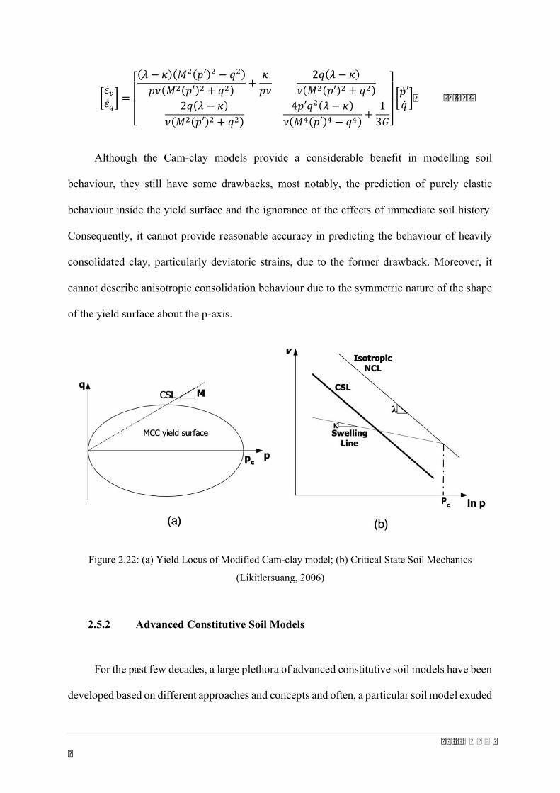
LIST OF FIGURES Figure 1.1: Requirements for construction in inappropriate ground profiles (Soil Stabilization System, viewed 22 November 2019, < https://allustabilization.wordpress.com/>) ............................................2 Figure 1.2: Long-term settlement issues highlighting the importance of modelling rate-dependent behaviour of soils (What Exactly Causes Foundation Settlement?, viewed 23 November 2019, < https://www.therealsealllc.com/what-exactly-causes-foundation-settlement>) ..................................9 Figure 2.1: Creep test performed at a low stress level: (a) Stress-strain relationship; (b) stress history; (c) strain history (after Wood, 1990) .................................................................................................... 16 Figure 2.2: Creep stages for a creep test performed by a triaxial apparatus: (a) Strain versus time; (b) log strain rate versus log time (after Augustesen et al. 2004) ............................................................. 17 Figure 2.3: Constant rate of strain (CRS) tests: (a) Strain history, and (b) stress-strain response (after Augustesen et al. 2004) ........................................................................................................................ 18 Figure 2.4: The results of the constant rate of strain tests on Batiscan clay (after Leroueil et al., 1985) .............................................................................................................................................................. 19 Figure 2.5: Stress-strain behaviour of Saint-Jean-Vianny Clay in undrained constant rate of strain tests (after Vaid et al., 1979) ................................................................................................................ 20 Figure 2.6: (a) Drained stress-strain curves for different constant rate of strain tests (𝑞𝐴, 𝑞𝐵, 𝑞𝑐 are peak strengths), (b) Strain rate effects on yield surface (after Augustesen et. Al, 2004) .................... 20 Figure 2.7: Ranges of strain rates in the in-situ state and laboratory tests (after Leroueil, 2006) ...... 21 Figure 2.8: Special constant rate of strain oedometer tests on Batiscan clay (after Leroueil et al., 1985) ..................................................................................................................................................... 22 Figure 2.9: (a) Types of compression curves dependent on the stress level (after Leroueil et al., 1985); (b) the corresponding strain rate (after Augustesen et al., 2004) ............................................ 23 Figure 2.10: Stress relaxation test (A→B): (a) Stress-Strain relationship; (b) strain history; (c) stress history (after Wood, 1990) ................................................................................................................... 24 Figure 2.11: Stress relaxation: (a) Stress-strain diagram for three different relaxation tests; (b) stress decay versus log time for the stress relaxation tests (after Augustesen et al. 2004) .......................... 25 Figure 2.12: Void ratio versus time for thick and thin samples using Hypothesis A (after Le et al. 2015) ..................................................................................................................................................... 26 Figure 2.13: Void ratio versus time for thick and thin samples using Hypothesis B (after Le et al. 2015) .............................................................................................................................................................. 26 Figure 2.14: Void ratio versus effective stress at the end of primary consolidation (after Jamiolkowski et al., 1985) ........................................................................................................................................... 28 Figure 2.15: Classification of Time-dependent soil models (after Liingaard et al., 2004) .................... 29 Figure 2.16: Definition of instant compression and delayed compression compared to primary and secondary compression (after Bjerrum, 1967): (a) the change in effective stress; and (b) compression versus time ............................................................................................................................................ 34 Figure 2.17: Bjerrum’s Time-line system (after Bjerrum, 1967) ........................................................... 35 Figure 2.18: Rheological Models: a) Maxwell model; b) Kelvin-Voigt model; and c) Bingham model 37 Figure 2.19: Rheological models proposed by Barden: (a) Barden’s proposed non-linear model; and (b) Barden’s simplified model (after Barden, 1965) (Note: N and L denote non-linear and linear, respectively) .......................................................................................................................................... 38 Figure 2.20: Rheological Model proposed by Rajot (1992) (after Perrone, 1998) ............................... 39

XIV

Figure 2.21: Schematic representation of typical rheological elements: a. Hookean linear spring; b. Viscous dashpot; and c. Plastic slider (after Liingaard et al, 2004) ...................................................... 39 Figure 2.22: (a) Yield Locus of Modified Cam-clay model; (b) Critical State Soil Mechanics (Likitlersuang, 2006) ............................................................................................................................. 43 Figure 2.23: Place of constitutive laws and physical principles in continuum mechanics (after Desai and Siriwardane, 1984) ......................................................................................................................... 44 Figure 2.24: Schematic representation of the Principles of Bounding Surface Plasticity (after Dafalias and Herrmann, 1982)............................................................................................................................ 46 Figure 2.25: Schematic representation of the Principles of Kinematic Yield Surface Plasticity (after Mroz, 1967 and Iwan, 1967) ................................................................................................................. 49 Figure 2.26: Schematic representation of the Overstress-type EVP Models (after Perzyna, 1963) .... 51 Figure 2.27: Schematic representation of the NSFS-type EVP Models (after Olszak and Perzyna, 1966) .............................................................................................................................................................. 53 Figure 3.1: (i) One-dimensional rheological model representing stored and dissipated plastic work; (ii) total stress-strain response; (iii) total stress-plastic strain response (after Collins, 2005) ............. 69 Figure 3.2: Schematic representation of the decomposition of the true stress into shift stress and dissipative stress components .............................................................................................................. 76 Figure 3.3: Flow Chart illustrating the steps in constructing the Incremental Form of the Elastic/Plastic Constitutive Law for the Development of Rate-independent Hyperplasticity Models 77 Figure 3.4: Flow Chart illustrating the steps in constructing the Incremental Form of the Elastic/Plastic Constitutive Law for the Development of Rate-dependent Hyperplasticity Models ... 84 Figure 3.5: Flow Chart highlighting the Similarities and Differences between Rate-independent and Rate-dependent Formulations for the Development of Hyperplasticity Models ................................ 86 Figure 4.1: Changes in the Shapes of Critical Surface in 𝑝′ − 𝑞 space, corresponding to the values of (a) 𝛾 and (b) 𝛼 varying over the range 1.0 to 0.1 ............................................................................... 106 Figure 4.2: Transformation of critical surface from (a) dissipative stress space to (b) true stress space ............................................................................................................................................................ 109 Figure 4.3: Changes in the Shapes of Critical Surface in 𝑝𝐷 − 𝑞𝐷 space, corresponding to the values of 𝛾 and 𝛼 varying over the range 1.0 to 0.1 (Using 𝛽 = 𝑡𝑎𝑛30°) .................................................... 121 Figure 4.4: Changes in the Shapes of Critical Surface in 𝑝𝐷 − 𝑞𝐷 space, corresponding to the values of 𝛾 and 𝛼 varying over the range 1.0 to 0.1 (Using 𝛽 = 0) .............................................................. 122 Figure 4.5: The effects of varying creep coefficient on the stress-strain behaviour using undrained triaxial test results on Haney clay ....................................................................................................... 133 Figure 4.6: Schematic representation of the behaviour of the Hyper-viscoplasticity model in 𝑝′ − 𝑞 space ................................................................................................................................................... 134 Figure 4.7: Definition of the parametric angle 𝜔 ............................................................................... 144 Figure 5.1: Comparison between the measured and predicted results for consolidated undrained shear test at a constant deviatoric stress rate on HKMD clay: (a) deviatoric stress 𝑞 versus axial strain 휀𝑎; and (b) effective stress paths ....................................................................................................... 148 Figure 5.2: Comparison between the measured and predicted results for two consolidated drained shear tests on HKMD clay: (a) deviatoric stress 𝑞 versus axial strain 휀𝑎; (b) volume strain 휀𝑣 versus axial strain 휀𝑎 and (c) effective stress paths ...................................................................................... 151 Figure 5.3: Comparison between the measured and predicted results for undrained triaxial tests on Osaka clay (Data from Adachi et al., 1995): (a) deviatoric stress 𝑞 versus axial strain 휀𝑎; and (b) effective stress paths .......................................................................................................................... 153

XV

Figure 5.4: Comparisons between the measured and predicted consolidated undrained triaxial test results on a mixture of kaolin and bentonite: (a) deviatoric stress 𝑞 versus axial strain 휀𝑎; (b) effective stress paths; and (c) axial strain 휀𝑎 versus pore-water pressure (𝑢) ................................. 156 Figure 5.5: Comparison between the measured and predicted results for the relationship between deviatoric stress 𝑞 and axial strain 휀𝑎 using undrained triaxial test results on Haney clay ............... 159 Figure 5.6: Comparison between the measured and predicted results for constant strain rate triaxial shearing tests on the HKMD under compression and extension tests: (a) normalised deviatoric stress 𝑞𝑝𝑐 versus axial strain 휀𝑎; and (b) normalised effective stress paths ............................................... 161 Figure 5.7: Comparison between the measured and predicted results for undrained triaxial tests for step-changed axial strain rate combined with stress relaxation on HKMD clay: (a) deviatoric stress 𝑞 versus axial strain 휀𝑎; (b) effective stress paths; and (c) axial strain 휀𝑎 versus pore-water pressure (𝑢) ....................................................................................................................................................... 164 Figure 5.8: Comparison between the measured and predicted results for K0-consolidated undrained triaxial CRS tests at an effective pressure of 75.4 kPa on soft Wenzhou Marine clay in extension: (a) effective stress paths; and (b) deviatoric stress 𝑞 versus axial strain 휀𝑎 ........................................... 167 Figure 5.9: Comparison between the measured and predicted results for K0-consolidated undrained triaxial CRS tests at an effective pressure of 150 kPa on soft Wenzhou Marine clay in compression: (a) effective stress paths; and (b) deviatoric stress 𝑞 versus axial strain 휀𝑎 ...................................... 168 Figure 5.10: Comparison between the measured and predicted results for K0-consolidated undrained triaxial CRS tests at an effective pressure of 150 kPa on soft Wenzhou Marine clay in extension: (a) effective stress paths; and (b) deviatoric stress 𝑞 versus axial strain 휀𝑎 .................... 169 Figure 5.11: Comparison between the measured and predicted results for K0-consolidated undrained triaxial CRS tests at an effective pressure of 300 kPa on soft Wenzhou Marine clay in compression: (a) effective stress paths; and (b) deviatoric stress 𝑞 versus axial strain 휀𝑎 ............... 170 Figure 5.12: Comparison between the measured and predicted results for K0-consolidated undrained triaxial CRS tests at an effective pressure of 300 kPa on soft Wenzhou Marine clay in extension: (a) effective stress paths; and (b) deviatoric stress 𝑞 versus axial strain 휀𝑎 .................... 171 Figure 5.13: Comparison between the measured and predicted results for K0-consolidated undrained triaxial compression tests on Shanghai soft clay: (a) effective stress paths; and (b) deviatoric stress 𝑞 versus axial strain 휀𝑎 ............................................................................................ 174 Figure 5.14: Comparison between the measured and predicted results for K0-consolidated step-changed axial strain compression test with unloading/reloading at effective pressure of 50kPa on HKMD clay: (a) deviatoric stress 𝑞 versus axial strain 휀𝑎; (b) axial strain 휀𝑎 versus pore-water pressure 𝑢 ........................................................................................................................................... 178 Figure 5.15: Comparison between the measured and predicted results for K0-consolidated step-changed axial strain compression test with unloading/reloading at effective pressure of 150kPa on HKMD clay: (a) deviatoric stress 𝑞 versus axial strain 휀𝑎; (b) axial strain 휀𝑎 versus pore-water pressure 𝑢 ........................................................................................................................................... 179 Figure 5.16: Comparison between the measured and predicted results for K0-consolidated step-changed axial strain compression test with unloading/reloading at effective pressure of 400kPa on HKMD clay: (a) deviatoric stress 𝑞 versus axial strain 휀𝑎; (b) axial strain 휀𝑎 versus pore-water pressure 𝑢 ........................................................................................................................................... 180 Figure 5.17: Comparison between the measured and predicted results for K0-consolidated step-changed axial strain extension test with unloading/reloading at effective pressure of 50kPa on HKMD clay: (a) deviatoric stress 𝑞 versus axial strain 휀𝑎; (b) axial strain 휀𝑎 versus pore-water pressure 𝑢 181

XVI

Figure 5.18: Comparison between the measured and predicted results for K0-consolidated step-changed axial strain extension test with unloading/reloading at effective pressure of 150kPa on HKMD clay: (a) deviatoric stress 𝑞 versus axial strain 휀𝑎; (b) axial strain 휀𝑎 versus pore-water pressure 𝑢 ........................................................................................................................................... 182 Figure 5.19: Comparison between the measured and predicted results for K0-consolidated step-changed axial strain extension test with unloading/reloading at effective pressure of 400kPa on HKMD clay: (a) deviatoric stress 𝑞 versus axial strain 휀𝑎; (b) axial strain 휀𝑎 versus pore-water pressure 𝑢 ........................................................................................................................................... 183

LIST OF TABLES

Table 2.1: Four possible forms of the free-energy potential function ..................................... 57 Table 3.1: Summary of Derivations for Rate-independent Hyperplasticity Framework ......... 73 Table 3.2: Summary of Derivations for Rate-independent Hyperplasticity Framework (Using Triaxial Notation)..................................................................................................................... 74 Table 3.3: Basic Formulations for Rate-independent Hyperplasticity Framework ................. 75 Table 3.4: Basic Formulations for Rate-dependent Hyperplasticity Framework .................... 83 Table 3.5: Comparisons between Rate-independent and Rate-dependent Formulations for the Development of Hyperplasticity Models ................................................................................. 85 Table 5.1: Values of Model Parameters for HKMD Clay, Osaka Clay and Kaolin and Bentonite Clay Mixture.......................................................................................................... 146 Table 5.2: Values of Model Parameters for Haney Clay and HKMD Clay .......................... 157 Table 5.3: Test Procedure for Step-changed Triaxial Shearing Test with Constant Strain Rate and Stress Relaxation on HKMD Clay .................................................................................. 162 Table 5.4: Values of Model parameters for Soft Wenzhou Marine Clay and Shanghai Soft Clay ........................................................................................................................................ 165 Table 5.5: Experimental Conditions for Undrained Triaxial Loading Tests on Shanghai Soft Clay ........................................................................................................................................ 173 Table 5.6: Values of Model Parameters for 𝐾0-consolidated HKMD Clay .......................... 176

XVII

Nomenclature & Abbreviations

Latin Notations

𝐴, 𝐵 functions for stress-like quantities

𝐶 secondary compression coefficient

𝐶 material constant controlling the extent of coupling

𝐶 swelling index 𝐶 compressive index

𝐷 relative contribution from the volumetric and deviatoric viscoplastic strains in determining the extent of coupling

𝐶 (휂) volumetric target value for 𝛽 𝐶 (휂) deviatoric target value for 𝛽

𝑒 initial void ratio 𝑒 void ratio 𝑒 reference void ratio ∆𝑒 change in void ratio 𝐹 overstress function 𝐺 elastic shear modulus 𝐺 initial elastic shear modulus 𝑔 elastic shear modulus gradient

XVIII

𝐽 cross-coupling elastic modulus 𝐾 elastic bulk modulus 𝑘 elastic bulk modulus gradient 𝑀 slope of the critical state line

𝑚 power value (material constant) representing the slope of the log 𝜇 − log 𝑒 curve

𝑛 power order (dimensionless material constant) 𝑝 effective stress �̇� change in effective stress 𝑝 reference mean stress 𝑝 effective stress at initial state (or reference time) 𝑝 pre-consolidation pressure �̇� change in pre-consolidation pressure 𝑝 initial pre-consolidation pressure 𝑝 volumetric shift stress 𝑝 volumetric dissipative stress 𝑄 viscoplastic potential function 𝑞 deviatoric stress �̇� change in deviatoric stress 𝑞 deviatoric shift stress 𝑡 reference time (or absolute equivalent time) 𝑉 specific volume 𝑤 liquid limit 𝑤 𝑤 𝑧

plastic limit flow potential function force potential function

Greek Notations

𝛿 Kronecker’s delta

𝛼 material constant linking to the amount of deviatoric dissipation

𝛽 cross-coupling between volumetric and deviatoric dissipation

휀 strain in axial direction 휀 strain in radial direction 휀 total strain tensor 휀 total volumetric strain

XIX

휀 total shear strain 휀̇ total volumetric strain increment 휀̇ total shear (or deviatoric) strain increment 휀 elastic strain tensor 휀 elastic volumetric strain 휀 elastic shear strain 휀̇ elastic volumetric strain increment 휀̇ elastic shear strain increment 휀 plastic strain tensor 휀 viscoplastic strain tensor 휀 viscoplastic volumetric strain 휀 viscoplastic shear (or deviatoric) strain 휀̇ viscoplastic volumetric strain increment 휀̇ viscoplastic shear (or deviatoric) strain increment 𝛾 material constant linking to the amount of stored plastic work 𝜅∗ slope of swelling line in ln 𝑣 − ln 𝑝 plot 𝜆∗ slope of normal consolidation line in ln 𝑣 − ln 𝑝 plot 휂 stress ratio 𝜇 creep coefficient 𝜇 initial creep coefficient

ϱ Thermodynamics-based overstress function (in true stress space)

ϱ Thermodynamics-based overstress function (in dissipative stress space)

𝜎 effective stress at a reference time 𝜎 effective stress in axial direction 𝜎 effective stress in radial direction 𝜈 Poisson’s ratio

𝛿Φ dissipation increment function Ψ Gibbs free-energy function Ψ Elastic Component of Gibbs free-energy function Ψ Viscoplastic Component of Gibbs free-energy function Ψ̇ the differential of the free-energy function 𝜓 viscosity function �̅� generalised stress tensor 𝜒 dissipative stress tensor

Common Acronyms

CRS Constant Rate of Strain

XX

CSL Critical State Line EVP Elastic-viscoplastic MCC Modified Cam-clay OCR Over-consolidation Ratio UTC Undrained Triaxial Compression (UTC) UTE Undrained Triaxial Extension

1 | P a g e

CHAPTER 1

INTRODUCTION

2 | P a g e

1.1 Background

As a result of rapid advancement in social, and infrastructural development of the world,

accompanying the massive growth in its population, there has been an alarming concern for

the availability of suitable types of soil for construction in recent years. As a consequence, it

has become increasingly likely that the relatively inappropriate construction areas, such as

lakes, river and coastal regions, are to be considered as alternative options for future

construction projects. The most prevalent type of soils found in these areas are mostly soft

clays, which exhibit low permeability and shear strength, with high compressibility. One of the

major challenges when dealing with soft soils in geotechnical engineering design and analyses,

is the long-term deformation associated with soft soils. Inevitably, the constitutive modelling

for the simulation of time-dependent behaviour of soft soils has captivated much attention in

the geotechnical research society. The prediction of time-dependent behaviour of geomaterials,

such as creep, stress-relaxation and strain-rate dependency, bears considerable importance,

particularly in the ground settlements, which in turn, may result in significant deformation in

the long-term.

Figure 1.1: Requirements for construction in inappropriate ground profiles (Soil Stabilisation System,

viewed 22 November 2019, < https://allustabilization.wordpress.com/>)

3 | P a g e

The experimental investigation of time-dependent deformation in a wide variety of

materials has been performed by numerous researchers, such as for frozen soils (Lai et al.,

2000; Liu et al., 2018), rock-like materials (Wang et al., 2015; Nguyen et al., 2017; Cao et al.,

2018; Zhao et al., 2018), asphalt concrete (Darabi et al., 2012a,b; Cheng et al., 2016), plasticine

materials (Feng et al., 2017) and polymeric materials (Ghorbel, 2008). In addition, a multitude

of geotechnical researchers have developed a plethora of constitutive soil models to consider

the time- and rate-dependent behaviour of clays, varying from simple Elastic-Plastic to Elastic-

Visco-Plastic (EVP) models (Kelln et al., 2008; Fatahi et al., 2013; Karim and Gnanendran,

2014; Azari et al., 2016; Le et al., 2015; Yin et al., 2015a,b). Yin (2006) has also discussed the

fundamental facts related to elastic viscoplastic modelling of the time-dependent stress-strain

behaviour of geomaterials and stated that the EVP models are more general than the traditional

elastic-plastic constitutive models. Among the abundance in a variety of constitutive models

for the time-dependent behaviour of soft soils, the EVP model proposed by Yin and Graham

(1989) is considered as simple yet practical for the numerical analyses related to long-term

settlement of soft soils. Afterwards, they have extended this model for triaxial and general

stress states with the adoption of the elliptical flow surface from Modified Cam-clay model,

and Mises failure criterion. However, the postulated linear logarithmic function results in the

creep strain being infinite as time approaches to infinity. In order to rectify this shortcoming,

Yin (1999) proposed a non-linear creep formulation with the introduction of creep coefficient

and stress-dependent creep strain limit. Although the non-linear creep model can reproduce

more accurate results in the simulation of long-term settlement of soft soils, the parameter

determination related to the non-linear creep parameters exhibited several restrictions for its

adoption in geotechnical applications. Notwithstanding this improvement, Yin et al. (2015a)

and Zhu et al. (2016a) pointed out that the non-linear creep formulation postulated by Yin

(1999) as being only applicable to one particular constant applied stress level, as the non-linear

4 | P a g e

creep coefficient did not continuously decrease with the void ratio when the applied stresses

were continuously increasing and hence, a negative void ratio could only be avoided under a

constant applied pressure. In order to address this shortfall, Yin et al. (2015a) have proposed

an improved non-linear creep formulation with consecutively decreasing consolidation

coefficient. Besides, Le and Fatahi (2016) have proposed a more rigorous numerical

optimisation technique, i.e. Trust-Region Reflective Least Square (TRRLS) approach and

applied the algorithm to obtain the EVP model parameters of the clay samples in the laboratory

conditions.

Concomitantly, Zhou et al. (2005) and Leoni et al. (2008) have extended the isotropic

creep models by Vermeer and Neher (1999) and Yin et al. (2002), in which the volumetric

viscoplastic strain remains constant on the yield surface, regardless of the stress state. This has

resulted in the unrealistic predictions of volumetric viscoplastic strains when the stress state

approaches the critical state line; instead, the value should be nearly zero based on the

laboratory measurements. In recent years, the modelling of combined anisotropic and

viscoplastic effects for clays (Yin et al., 2010; Sivasithamparam et al., 2015; Jiang et al., 2017;

Leal et al., 2017; Castro et al., 2018), along with the consideration of strain rate and temperature

(Leroueil and Marques, 1996; Laloui et al., 2008) or strain rate and structure (Hinchberger et

al., 2010; Yin and Karstunen, 2011; Zhang, 2018) have also been carried out.

Overall, it has been acknowledged that most of the existing viscoplastic constitutive

models have been based on the elastic viscoplastic modelling (EVP) framework (Perzyna,

1963; 1966) or the non-stationary flow surface framework (Naghdi and Murch, 1963; Olszak

and Perzyna, 1970). The most profound impediment in the overstress-based models stems from

the arbitrariness of the postulated overstress function. Moreover, they do not satisfy with the

consistency condition and it is also difficult to justify their compliance with the fundamental

laws of thermodynamics.

5 | P a g e

Besides, although all these models have enlightened the understanding of time-dependent

behaviour of soils, they still have their own deficiencies. The most profound limitations are the

basic assumption of the flow surface being elliptical as defined in Modified Cam-clay (MCC)

model, developed by Roscoe and Burland (1968), the flow rule being associated, and the elastic

behaviour being strictly isotropic. Moreover, they often require a considerable number of

assumptions without being related to the physical phenomena of real soils.

1.2 Problem Statement

It is important to acknowledge that the most important attribute of the constitutive models

is their compliance with the physical phenomena. The fact that they must obey certain

principles or axioms that govern the physical phenomena, such as conservation of mass,

conservation of energy and the fundamental laws of thermodynamics, should be emphasised.

Taking this into strong consideration, the aforementioned constitutive frameworks do not take

into account of the fundamental laws of thermodynamics and they may eventually violate one

or the other physical phenomena. According to Houlsby and Puzrin (2006), the constitutive

models that do not comply with the laws of thermodynamics may not be used with any

confidence to predict the material behaviour.

To circumvent the problem of having a substantial number of assumptions and using ‘ad

hoc’ procedures, the major objective of this research is to develop a constitutive soil model

based on the laws of thermodynamics, from which the constitutive behaviour of soils is derived

in a systematic procedure. Accordingly, the extraction of plasticity theory with the major

emphasis on the fundamental laws of thermodynamics was originated from the early works of

Halphen and Nguyen (1974) and Ziegler (1983), in which the derivation of the entire

6 | P a g e

constitutive response for predicting stress-strain behaviour of plastic materials is based on two

scalar thermodynamic potential functions. Considerably, this is a relatively new approach to

the development of elastic-plastic constitutive models, which was termed ‘hyperplasticity by

Collins and Houlsby (1997) and Houlsby and Puzrin (2000, 2006) for the modelling of time-

independent behaviour of soils. Collins and Houlsby (1997) discussed the application of

thermomechanical principles to the modelling of geotechnical materials and emphasised on the

mathematical technique, called Legendre transformation, in developing rate-independent

hyperplasticity models.

During recent years, a few attempts have been made for the extension towards rate-

dependent behaviour of soils (Vlahos et al., 2006; Likitlersuang and Houlsby, 2007; Puzrin and

Rabaiotti, 2009; Zhang, 2017; Zhang and Buscarnera, 2017), frozen soils (Zhou et al., 2016),

peat (Boumezerane et al., 2015), rubbers (Guo et al., 2018), polymeric materials (Gudimetla

and Doghri, 2017) and steel behaviour (Benaarbia et al., 2018). Moreover, Abu Al-Rub and

Darabi (2012) have proposed a thermodynamic-based framework for the constitutive

modelling of temperature-, time- and rate-dependent behaviour of viscous materials and Zhu

et al. (2016b) have presented a coupled EVP model based on thermodynamics to predict the

cyclic deformation of metals. Furthermore, Darabi et al. (2012a; b) have adopted the former

approach to simulate the behaviour of asphaltic materials over a wide range of time- and rate-

dependent experiments. Recently, Darabi et al. (2018) have further discussed on a

thermodynamic-based approach to systematically derive generalised non-associative rate-

independent and rate-dependent plasticity theories. However, most of the existing

thermodynamic-based models often require a substantial number of parameters and they still

adopt the aforementioned limitations, such as the assumption of the flow rule being associated

and the shape of the yield surface being adopted as symmetric elliptical one defined in the

MCC model, without considering the possibilities of deformed shapes of the yield surface.

7 | P a g e

As suggested by the laboratory experiments presented in Dafalias and Taiebat (2013;

2014) and Zhou et al. (2017), the yield loci not only expand but also translate in the stress space

and the shapes of the yield loci do vary depending on the types of soils. In order to address the

experimental findings, Mroz (1998) introduced the kinematic hardening mechanism to the

constitutive modelling of soils, along with the hardening function, in order to control the

movement and the variation in size of the yield loci. Kinematic hardening during inelastic

deformations is usually described by a so-called ‘back’ or ‘shift’ stress, which is considered as

an internal variable, for which an adequate constitutive equation is formulated (Sansour et al.,

2006). Recently, Zhou et al. (2018) have proposed a kinematic hardening EVP constitutive

model, adopting Perzyna's overstress theory, to predict the stress- strain behaviour of saturated

cohesive anisotropic soils. However, their EVP model still employs associated flow rule and

requires a sizeable number of parameters based on a considerable number of assumptions.

From the perspective of hyperplasticity, the kinematic hardening behaviour is considered in

the form of ‘shift’ stress, referred to as ‘stored plastic work’, which is determined by the

additional plastic free-energy function, i.e. not contributing to the plastic dissipation. It is to be

emphasised here that some portion of the plastic work is stored in the form of continuum plastic

strain (i.e. the residual strain when a continuum element is unloaded back to a particular

predefined reference loading condition due to the inhomogeneous nature of the micro-level

deformation). Consequently, some of the micro-level elastic energy is ‘frozen’, resulting in

recoverable stored plastic work (Collins, 2005). This contradicts the conventional perfect

plasticity theory, which often assumes that the ‘plastic work’ and ‘plastic dissipation’ are equal

(i.e. all the plastic work is assumed to be dissipated). Most importantly, this kinematic

hardening behaviour has not been widely considered in modelling the viscoplastic stress-strain

behaviour of soils.

8 | P a g e

1.3 Research Objectives and Scope

This research is a rational effort in adopting the conservative thermodynamics-based

hyperplasticity concept to propose a simple yet versatile constitutive soil model to simulate the

non-linear creep behaviour, along with the incorporation of both isotropic and kinematic

hardening effects. Due to the important fact that the hyperplasticity theory is mainly based on

the fundamental laws of thermodynamics, it also avoids the need to introduce a considerable

number of ‘ad hoc’ assumptions without being related to the physical phenomena of soils. One

of the key benefits bears in the development of relatively rigorous, compact and consistent

constitutive framework, as the resulting model cannot produce thermodynamically

unreasonable outcomes. The proposed model is developed in a relatively succinct mathematical

form, as the entire constitutive response is determined through the specification of two scalar

thermodynamic potential functions, i.e. the free-energy and dissipation potential functions,

using a systematic standardised procedure. These two fundamental potential functions are

related through Legendre transformation, which results in the natural incorporation of non-

associated flow, which is now widely regarded as a proper approximation for improved

predictions in the behaviour of soils, being derived logically and naturally without postulating

any further potential functions, which are usually introduced to arbitrate the associativity of the

flow rule in conventional plasticity theory. In addition, the proposed model takes into account

of kinematic hardening behaviour of soils in the form of ‘shift’ stress within the context of

hyperplasticity. It is emphasised that not all the plastic work is dissipated; but some portion is

stored when an element is unloaded back to a predefined reference stress level at the continuum

level (Lai et al., 2014). As a result, the kinematic hardening behaviour is modelled by

incorporating a ‘back or shift stress’, as part of the additional viscoplastic component of the

free-energy function into the proposed model. The extended thermodynamic potential

9 | P a g e

functions are postulated, considering the variation in shapes of the yield loci, for the simulation

of time- or rate-dependent stress-strain behaviour of soils.

Figure 1.2: Long-term settlement issues highlighting the importance of modelling rate-dependent

behaviour of soils (What Exactly Causes Foundation Settlement?, viewed 23 November 2019, <

https://www.therealsealllc.com/what-exactly-causes-foundation-settlement>)

Furthermore, the proposed model has been extended to incorporate the effects of the

arrangement of particles and the interparticle bonding, i.e. termed as ‘structure’ by Mitchell

(1993; 1956), which was also referred to as “fabric” by Muhunthan et al. (1996). Considering

the importance of acknowledging the effects of the interparticle bonding of particles and their

arrangement, particularly in natural soils, the current study furthers in a radical extension of

the proposed model to incorporate the consideration of ‘fabric’ effects on the time-dependent

stress-strain behaviour of natural soils. The extended model intends to capture the loading-rate

or strain-rate dependent behaviour of soils, considering the variations in the fundamental

shapes of critical surface with a β-line defining the inclination of the non-symmetrical elliptical

10 | P a g e

critical surface in the 𝑝 -𝑞 plane, along with rotational, kinematic hardening effects and non-

associated behaviour, derived as a natural consequence of this approach.

The proposed model’s predictions demonstrate the capability and versatility in

reproducing the viscous behaviour of soft soils, including natural ones, under different loading

conditions, which has been validated by using comparisons with the existing triaxial and

oedometer laboratory measurements available in the literature.

1.4 Organisation of Thesis Structure

The composition of the thesis comprises of six key chapters, which can be described as

follows:

Chapter 1 presents a brief introductory background on the constitutive modelling of

stress-strain behaviour of soils, along with the problem statement, the major objectives and

scope of the current study.

Chapter 2 describes a comprehensive literature review on the real soil behaviour and the

importance of modelling time-dependent viscoplastic behaviour of geomaterials, particularly

soils. Moreover, the challenges associated with the development of constitutive soil models

and the distinctive characteristics of the existing advanced constitutive modelling frameworks

are also presented to emphasise on the problem statement of the current study.

In Chapter 3, the underlying principles of the Hyperplasticity theory, signifying its

essential components and requisite foundation towards the development of a new Hyper-

viscoplasticity theory have been elaborated. Moreover, the fundamental laws of

thermodynamics have been discussed. This has been accompanied by the practical summary

11 | P a g e

of rate-independent hyperplasticity approach, from which the rate-dependent hyperplasticity

framework has been built upon using a constructive and consistent approach and thus,

highlighting the rigidity, compactness and reliability acting as a strong foundation for the

development of hyper-viscoplastic soil models in the current study.

Chapter 4 proposes a novel mixed hardening hyper-viscoplasticity model to simulate the

time- or rate-dependent stress-strain behaviour of soils, along with the consideration in varying

shapes of the yield loci by pursuing non-associated flow and accounting for kinematic

hardening effects. The important characteristics of the proposed model, including the non-

associated flow rule derived as a natural consequence, rather than imposed arbitrary application

compared with the traditional viscoplasticity models, the postulated additional viscoplastic

free-energy function and the dissipation potential function, along with the hypothesised non-

linear creep formulation based on experimental findings, are provided and further elaborated

in details. Moreover, the proposed model is extended to account for the effects of the

combination of the arrangement of particles and the interparticle bonding, particularly crucial

in modelling stress-strain behaviour of natural soils. The extended aspects of the free-energy

and dissipation potential functions, from which the rotational, kinematic hardening law stems

from the additional viscoplastic free-energy potential, are elaborated and discussed in details.

In Chapter 5, the summary and related procedures to determine the required model

parameters have been extensively elaborated. The proposed H-Creep model requires 10 model

parameters in total, whereas the extended model introduces only one additional parameter

compared to its original counterpart, resulting in a relatively straightforward parameter

determination procedure, which has been discussed. Accordingly, the proposed and extended

models are applied to a wide range of laboratory experiments, including the normally

consolidated, overconsolidated and 𝐾 -consolidated undrained strain-controlled and stress-

controlled triaxial compression and extension tests, undrained triaxial shearing tests with

12 | P a g e

stress-relaxation and constant rate of strain tests. Moreover, the comparisons between the

numerical simulations and the laboratory measurements, are performed to investigate the

validity and performance of the proposed and extended models in reproducing the viscous

behaviour of soft soils, including natural ones, under a variety of loading conditions.

Chapter 6 summarises the significant findings of this research, together with the main

concluding remarks and recommendations for further research. This is followed by the

Appendix sections elaborating further details to supplement the important findings throughout

this research.

13 | P a g e

CHAPTER 2

LITERATURE REVIEW

14 | P a g e

2.1 Introduction

For several decades, time-dependent behaviour of soils has been a debatable subject for

many researchers in the area of geotechnical engineering. It has been widely acknowledged

that Terzaghi’s classical theory of one-dimensional consolidation, published in 1943, can

provide a reasonable approximation of the settlement induced by the pore water pressure

dissipation. Although the conventional or simplified methods can offer an appropriate

estimation of the settlement of soils in relatively simple soil scenarios, they cannot be applied

to predict the complicated real soil behaviour, such as the relationship between stress-strain-

strain rate or the effects of temperature. This chapter presents a review on the importance of

understanding the real soil behaviour, along with the most crucial time-dependent aspects

observed in relation to the mechanical behaviour of soils. Moreover, the time-dependent

behaviour of geomaterials, including creep, stress relaxation and strain-rate dependency are

discussed. Furthermore, the significance of capturing such behaviour of geomaterials,

particularly soils, and the challenges associated with the development of constitutive soil

models are investigated. In addition, a number of the existing advanced constitutive soil models

are examined and elaborated in details.

2.2 Real Soil Behaviour

In stark contrast to reality, the material behaviour is still often assumed to be linear elastic

in most of the geotechnical analyses of engineering problems. However, real soils do not

simply behave linear elastically and the understanding of real soil behaviour is extremely

crucial to achieve a reasonable level of accuracy in predicting the associated stress-strain

characteristics. The non-linearity is highly present in the real soil behaviour, i.e. both strength

15 | P a g e

and stiffness are dependent on the stress and strain level. Therefore, considerable knowledge

and understanding is important to identify some important aspects of these complicated soil

behaviour before delving into the development of constitutive models.

In general, the stress-strain characteristics of soils should fall into the following

categories. For elastic material behaviour, the strain follows the stress immediately, and

becomes zero after the removal of stress. For elastoplastic material behaviour, the strain also

follows the stress immediately, but there is some permanent strain after stress release. For

viscoelastic material behaviour, the strain shows time delayed response on a stress step,

indicating the time-dependent behaviour. For viscoplastic material behaviour, the time-

dependent behaviour is accompanied by permanent strain.

2.3 Time-dependent Behaviour of Soils

Another major aspect in modelling soil behaviour is that soils exhibit time-dependent

behaviour as well as plastic deformation. It is commonly understood that time-dependent

settlement in soils, for instance, saturated clay, results mainly due to two important factors: (i)

volume changes due to viscous deformations, and (ii) volume changes due to pore-water

dissipation. Consequently, soils are also called as viscous material. The viscous properties

define the time dependence of the state of stress and strain, whilst plastic properties make these

states depend on the loading path. This section describes the important constituents of the time-

dependent settlement of soft soils, such as time effects, strain rate effects and stress

dependency.

16 | P a g e

2.3.1 Creep

When soil is subjected to a constant load, it will deform over time and this phenomenon

is called creep. As demonstrated in Figure 2.1, a creep test is performed at a low stress level

following a strain path from point 1 to point 2. Consider, a soil is sheared to the stress-strain

state at point 1, from which creep is commenced with the constant stress, as shown in Figure

2.1b. As depicted in Figure 2.1c, the strain state progress to point 2, as the strain is gradually

increasing.

Figure 2.1: Creep test performed at a low stress level: (a) Stress-strain relationship; (b) stress history;

(c) strain history (after Wood, 1990)

2.3.2 Stages of Creep Process

The creep response under a constant effective stress performed using triaxial apparatus

can be classified into three main components: i) primary or transient creep; ii) secondary or

stationary creep; iii) tertiary or acceleration creep. The primary stage of creep is referred to as

the transient creep corresponding to the decreasing strain rate, while the secondary and tertiary

creep stages are the stationary creep with constant creep strain rate and the acceleration creep

with the increasing strain rate, respectively. The tertiary creep phase gradually and eventually

Strain (휀)

1 2 1 2

Time (𝑡)

1

2

Stress (𝜎) Strain (휀)

Time (𝑡)

Stress (𝜎)

a) b) c)

17 | P a g e

leads to the creep rupture or creep fracture of soils, as observed in the triaxial creep tests

(Augustesen et al. 2004). The corresponding creep test results can be depicted in either a strain

vs time graph or logarithm of strain rate vs logarithm of time graph, as shown in Figure 2.2.

Figure 2.2: Creep stages for a creep test performed by a triaxial apparatus: (a) Strain versus time; (b)

log strain rate versus log time (after Augustesen et al. 2004)

In drained creep tests, the effective stresses, i.e. the mean effective stress 𝑝 and the

deviatoric stress 𝑞, are kept constant. In undrained creep tests, 𝑝 decreases due to increase in

pore pressure, while the deviatoric stress 𝑞 remains constant. Therefore, only the drained creep

represents a pure creep process, as pointed out in Augustesen et al. (2004).

2.3.3 Strain Rate Effects

As pointed out in a number of researchers, such as Leroueil et al. (1985), Mesri and Feng

(1986) and Jia et al. (2010), strain rate is another significant factor that influences the time-

dependent compressibility of soft soils. In order to study the stress-strain-time relationship at

different strain rates, Constant Rate of Strain (CRS) consolidation tests have been broadly

employed, from which a unique relationship is found among stress-strain-strain rate, suggested

by Leroueil et al. (1985). As emphasised in Feng (1991), a CRS test can provide more direct

(𝑡)

(휀)

Primary Secondary

Tertiary

Rupture

𝑙𝑜𝑔(𝑡)

𝑙𝑜𝑔(휀̇)

Primary Secondary

Tertiary

Rupture

a) b)

18 | P a g e

and accurate relationship between stress-strain, as the stress-strain curve can be continuously

monitored. In general, a larger strain rate results in a higher effective stress at a certain strain

and hence, the stiffness of soil increases with the increasing strain rate (Augustesen et al. 2004).

Moreover, the influence of the strain rate on the pre-consolidation pressure is also observed.

2.3.3.1 Constant Rate of Strain (CRS) Tests

In a constant rate of strain (CRS) test, the total strain rate is kept constant throughout the

test, while the stress is then monitored to determine the stress-strain relationship. In general, it

can be observed that the effective stress at a constant strain rate increases with the increase in

the loading rate, as depicted in Figure 2.3. In other words, the stiffness of the soil increases

with the rising strain rate (Augustesen et al. 2004).

Figure 2.3: Constant rate of strain (CRS) tests: (a) Strain history, and (b) stress-strain response (after

Augustesen et al. 2004)

Although CRS tests have some advantages compared to the standard oedometer tests,

particularly in the relatively shorter test duration required for CRS tests, the major challenge

in CRS tests is the difficulty in the selection of the imposed strain rate to obtain an appropriate

stress-strain curve as an output. Hence, it is crucial to emphasise that a rational imposed strain

휀̇ < 휀̇ < 휀̇ Stress (𝜎)

휺̇ퟏ

휀̇

휀̇ Strain(휀)

Time(𝑡)

휺̇ퟏ

휺̇ퟐ 휺̇ퟑ

Strain(휀) a) b)

19 | P a g e

rate, based on the conventional primary consolidation data, is necessary in order to determine

the information related to End of Primary (EOP) consolidation stress-strain relationship.

According to Leroueil et al. (1985), a unique relationship among stress – strain – strain

rate is observed from a series of CRS tests, in one-dimensional and triaxial conditions, on

Batisan clay (shown in Figure 2.4). Due to the fact that the stress-strain curve can be

continuously monitored, the stress-strain relationship obtained from a CRS test is more direct

and accurate (Feng, 1991). Figure 2.5 demonstrates the influence of strain rate on the stress-

strain behaviour of overconsolidated Saint-Jean-Vianny clay, from the CRS tests conducted by

Vaid et al. (1979). Furthermore, Figure 2.6 depicts the effects of various constant strain rates

on peak strength and the size of the yield surface, as discussed in Augustesen et al. (2004).

Figure 2.4: The results of the constant rate of strain tests on Batiscan clay (after Leroueil et al., 1985)

As shown in Figure 2.6, the corresponding yield surface related to the particular constant

strain rate is denoted as ‘static yield surface’, which is one of the vital ingredients in the existing

Batiscan CRS tests Strain rates: s-1

휀̇ = 1.43 × 10⁻⁵ 휀̇ = 5.30 × 10⁻⁶

휀̇ = 2.13 × 10⁻⁶

휀̇ = 5.33 × 10⁻⁷

휀̇ = 1.07 × 10⁻⁷

휀̇ = 1.69 × 10⁻⁸

휺̇풛ퟏ

휺̇풛ퟐ

휺̇풛ퟑ

휺̇풛ퟒ

휺̇풛ퟓ

휺̇풛ퟔ

휺̇풛ퟔ 휺̇풛ퟏ

휺̇풛ퟐ

휺̇풛ퟑ

휀̇ , 휀̇ , 휀̇

𝜎 [𝑘𝑃𝑎]

휀 [ %

]

∆풖 [ 풌

𝑷풂]

0

10

0

20

15

25

5

50 100 150 200 250

20 | P a g e

constitutive EVP models developed based on Perzyna’s overstress theory (discussed in details

in the next section).

Figure 2.5: Stress-strain behaviour of Saint-Jean-Vianny Clay in undrained constant rate of strain tests

(after Vaid et al., 1979)

Figure 2.6: (a) Drained stress-strain curves for different constant rate of strain tests (𝑞 , 𝑞 , 𝑞 are

peak strengths), (b) Strain rate effects on yield surface (after Augustesen et. al, 2004)

휀̇1 = 2.8 × 10⁻¹ %/min 휀̇2 = 5.30 × 10⁻⁶ %/min 휀̇3 = 2.13 × 10⁻⁶ %/min

휀̇

휀̇

𝑞, kPa

휀 , %

휀̇

700

600

500

400

300

200

100 0 0.5 1.0 1.5 2.0 2.5 3.0 3.5

21 | P a g e

According to Leroueil (2006), the range of strain rates for different soils in in-situ state

for corresponding strain rates from different laboratory measurements are shown in Figure 2.7.

As demonstrated in Figure 2.7, the strain rates corresponding to the 24-hour incremental

loading tests are relatively closer to the strain rates compared to the strain rates obtained from

other tests.

Figure 2.7: Ranges of strain rates in the in-situ state and laboratory tests (after Leroueil, 2006)

2.3.3.2 Change in Rate of Strain Tests

As in the CRS tests, a unique relationship is also obtained among the effective vertical

stress, strain and strain rate in the specialised CRS tests, in which the strain rates are changed

at various strain and maintained for a period of time. Based on the two tests conducted by

Leroueil et al. (1985) on Batisan clay, the influence of the change in strain rate is continuous

and the resulting curve stays on the same stress-strain graph during the step-changed strain rate

tests, as shown in Figure 2.8.

22 | P a g e

2.3.4 Stress Effects

Depending on the applied stress level, three important types of time-depending

compression curves are identified:

Figure 2.8: Special constant rate of strain oedometer tests on Batiscan clay (after Leroueil et al., 1985)

i) When the final effective stress is less than the pre-consolidation pressure, the

compression is not significant and the slope of the compression curve progressively

increases after EOP, as in the case of overconsolidated soils in Figure 2.9. The slope

of the corresponding strain rate curve decreases linearly with time.

ii) When the final effective stress is approximately equal to the pre-consolidation

pressure, the slope of the compression curve after the EOP is higher than the

corresponding value observed in Type (i). When the effective stress increases from

the overconsolidated range to the normally consolidated range, similar compression

curve is observed.

iii) When the effective stress is within the normally consolidated range, as commonly

observed in the behaviour of soft soils, the compression is excessive during the

0 5

10

15

20

0 50 100 150 200 250

Batiscan CRS tests

Strain rates: s-1

── Special test 1 ---- Special test 2

휀̇ = 2.70 × 10⁻⁶

휀̇ = 1.05 × 10⁻⁷

휀̇ = 1.34 × 10⁻⁵

𝜎 [𝑘𝑃𝑎]

휺 풛 [ %

]

휺̇풛ퟐ

휺̇풛ퟐ

휺̇풛ퟐ

휺̇풛ퟐ

휺̇풛ퟏ

휺̇풛ퟏ

휺̇풛ퟏ

휺̇풛ퟏ

휺̇풛ퟑ

23 | P a g e

excess pore water pressure dissipation, and the slope of the corresponding strain

rate curve after EOP keeps decreasing with time.

Figure 2.9: (a) Types of compression curves dependent on the stress level (after Leroueil et al., 1985);

(b) the corresponding strain rate (after Augustesen et al., 2004)

2.3.5 Stress Relaxation

Stress relaxation is a process, in which the decrease in effective stress with time at a

constant value of strain. As depicted in Figure 2.10, a stress relaxation test is conducted, in

which the stress relaxation process is commenced at Point 1 by maintaining the identical total

strain over a certain time period. As time progresses, the stress-strain rate moves towards Point

2. During this process, the gradual decrease in effective stress is observed, which is called stress

relaxation.

Stress relaxation tests are usually conducted using triaxial apparatus in order to observe

the variation in the deviatoric stress under constant strain level (Drumright and Nelson, 1985;

Yin and Cheng, 2006). Based on the observations discussed in Silvestri et al. (1988), the

deviatoric stress reached the stabilised stress relaxation level in less than 1 day from the stress

relaxation tests performed on Louiseville clay. Based on the observation and the analysis of

24 | P a g e

several triaxial stress relaxation test data, the normalised deviatoric stress 𝑞 𝑞⁄ , i.e. the ratio

of the deviatoric stress 𝑞 at time 𝑡 and the deviatoric stress at the beginning of stress relaxation

𝑞 , decreases linearly with the increase in logarithm of time after an initial time period, as

shown in Figure 2.11 (Lacerda and Houston, 1973).

Figure 2.10: Stress relaxation test (A→B): (a) Stress-Strain relationship; (b) strain history; (c) stress

history (after Wood, 1990)

Moreover, Yin and Cheng (2006) also observed that the corresponding strain rate at the

beginning of the test had an impact on when the stress-relaxation commenced from the triaxial

tests performed on Hong Kong marine clay. Hence, it can be concluded that the slower the

initial strain rate, the longer it takes for the stress relaxation process to commence (Lacerda and

Houston, 1973). Similar laboratory observations were also reported in Graham et al. (1983)

and Fodil et al. (1997). It was suggested that the curve joining the stress relaxation states would

represent a “static effective stress state”, analogic to the term “static yield surface” in the

Perzyna’s overstress theory (Perzyna 1963; 1966). Furthermore, it was observed that the excess

pore water pressure remained almost constant during the undrained stress relaxation tests, as

stress relaxation tests were mostly conducted under undrained conditions (Lacerda and

Houston, 1973; Sheahan et al. (1994)).

Time (𝑡)

1

2

1 2

Time (𝑡)

1

2

Strain (휀) Stress (𝜎)

Time (𝑡)

Stress (𝜎)

a) b) c)

25 | P a g e

Figure 2.11: Stress relaxation: (a) Stress-strain diagram for three different relaxation tests; (b) stress

decay versus log time for the stress relaxation tests (after Augustesen et al. 2004)

2.3.6 Consolidation and Creep – Hypotheses A and B

In the past several decades, a plethora of approaches have been developed for the

simulation of time-dependent behaviour of soft soils. In the existing EVP models, some

researchers have insisted that the total strain rate is decomposed into elastic strain rate, plastic

strain rate and viscoplastic strain rate, whilst others have considered that the total strain rate is

divided into elastic strain rate and viscoplastic strain rate. The former approach is so-called

Hypothesis A, and the latter is denoted as Hypothesis B, respectively. Hypothesis A mainly

assumes that creep only occurs after the end of primary consolidation, i.e. after complete

dissipation of pore water pressure. Hypothesis A has been adopted in Ladd et al. (1977), Mesri

and Godlewski (1977), and Mesri and Choi (1985). Hypothesis A has suggested that the value

of void ratio at the end of primary consolidation (𝑒 ) is unique regardless of the thickness of

the soil sample, drainage conditions and loading duration. Although the time taken to reach the

end of primary consolidation (𝑡 ) is longer for the thick sample compared to that of the thin

sample, the void ratios of both samples remain the same, as illustrated in Figure 2.12.

풍풐품(풕)

(풒)

(휺)

휺̇ퟏ

휺̇ퟐ 휺̇ퟑ

휀̇ > 휀̇ > 휀̇ = strain rate prior to relaxation

𝑞/𝑞

휺̇ퟏ 휀̇ 휀̇

1.0

a) b)

26 | P a g e

Figure 2.12: Void ratio versus time for thick and thin samples using Hypothesis A (after Le et al.

2015)

Figure 2.13: Void ratio versus time for thick and thin samples using Hypothesis B (after Le et al.

2015)

In Hypothesis B, it is assumed that secondary compression occurs during the whole

consolidation process. Hypothesis B has been supported by Suklje (1957), Bjerrum (1967),

Leroueil et al. (1985) and Yin (1999). In contrast to Hypothesis A, Hypothesis B insists that

the longer it takes to reach the end of primary consolidation results in more compression under

27 | P a g e

a particular effective stress. Therefore, the void ratio at 𝑡 (i.e. 𝑒 ) for a particular applied

stress depends on the thickness of the soil sample, drainage conditions and loading duration.

Consequently, the 𝑒 of thin sample tends to be higher compared to that of the thick sample

due to its shorter drainage path and 𝑡 , as depicted in Figure 2.13.

According to Ladd et al. (1977), the compression curves for both thin and thick samples

merge together with time. In contrast, Aboshi (1973) suggested that the compression curve

after the end of primary consolidation continue to be parallel, based on the laboratory

observations.

As a result, two suggestions potentially exist at the end of primary consolidation:

1) Both compression curves merge together with time

2) Both compression curves continue to be parallel with time

Figure 2.14 further illustrates the contradicting nature of Hypotheses A and B based on

the compression curves at the end of primary consolidation. The adoption of Hypothesis A

results in a unique 𝑒 , thus leading to a unique value of pre-consolidation pressure (𝜎 ) for

a particular soil. In contrast, the adoption of Hypothesis B results in the reduction of pre-

consolidation pressure (𝜎 ) due to the accumulation of secondary compression with the

increasing thickness of the sample; hence, causing the EOP stress-strain curve to shift

downward, as portrayed in Figure 2.14.

Therefore, the major difference between Hypotheses A and B is the influence of the soil

sample thickness on the induced secondary compression with time. As indicated in Figure 2.14,

the thickness of the soil sample has a significant influence on the pre-consolidation pressure,

drainage path and 𝑡 , and hence, on the predictions of the total settlement. However, the real

28 | P a g e

soil behaviour lies somewhere between these two extreme hypotheses A and B, based on the

experimental observations performed by Aboshi (1973).

Figure 2.14: Void ratio versus effective stress at the end of primary consolidation (after Jamiolkowski

et al., 1985)

2.4 Modelling Time-dependent Behaviour of Soils

As proved in Casagrande and Wilson (1951), Tavenas et al. (1978) and Graham, Crooks

and Bell (1983), the observed stress-strain behaviour of clays and natural soils is time-

dependent. Moreover, Bjerrum (1967) pointed out that the time dependency on the stress-strain

behaviour of soils, especially highly plastic clays, is generally too significant to be ignored.

Therefore, the constitutive modelling of time-dependent behaviour of soils has attracted much

attention towards the geotechnical research community in the past decades. As a variety of

mathematical models have been developed to capture the time-dependent effects in geological

29 | P a g e

materials, particularly soils, these can be categorised into three major approaches; (i) the

empirical models, the rheological models, and general constitutive stress-strain-time/strain rate

models, as shown in Figure 2.15 (Liingaard et al., 2004).

Figure 2.15: Classification of Time-dependent soil models (after Liingaard et al., 2004)

2.4.1 Empirical Soil Models

The empirical laws are directly obtained by fitting experimental data from creep, stress

relaxation, and CRS tests in order to develop empirical relations to describe the time-dependent

behaviour of soils. In general, these constitutive relationships are expressed in closed-form

solutions or differential equations. The empirical relationships usually provide a reasonable

approximation of the behaviour of soils and a good foundation for developing more

sophisticated constitutive soil models. However, the arbitrary functions are strictly limited to a

specific boundary and loading conditions, together with the time spans of a particular

experiment, from which they are derived. Therefore, the empirical models are applicable to

engineering problems, especially due to their simplicity, as long as the boundary conditions

30 | P a g e

comply with the ones in the laboratory experiments. According to Liingaard et al. (2004), the

empirical models are classified as primary empirical relations and secondary semi-empirical

relations.

2.4.1.1 Primary Empirical Models

The primary empirical relationships are generally derived from the fitting of observed

laboratory data with simple mathematical functions, which can reproduce the actual behaviour

of the test sample. However, they are often strictly limited to specific test phenomena. The

empirical relations for creep are most commonly based on the semi-logarithmic law, which

describes the secondary compression observed in oedometer tests against the logarithm of time.

One of the most common and simplest empirical models is based on the concept of

constant coefficient of secondary compression 𝐶 or 𝐶 , defined in Mesri and Godlewski

(1977) and Terzaghi and Karl (1996) as follows:

𝐶 =∆𝑒

∆ log 𝑡 𝑜𝑟 𝐶 =𝐶

1 + 𝑒 (2.1)

where, 𝑒 is defined as initial void ratio and ∆𝑒 is the change in void ratio. The parameters

𝐶 and 𝐶 are the coefficients of secondary compression with respect to 𝑒 and 휀, respectively.

This empirical relationship in Equation (2.1) was modified by Ladd et al. (1977), to

estimate the secondary settlement, as follows:

𝐶 =𝐶

1 + 𝑒 and 𝑆 = 𝐶 𝐻 ∙ log𝑡𝑡 (2.2)

On the other hand, Walker and Raymond (1968) defined the compression index from the

laboratory tests on sensitive Leda clay, as follows:

31 | P a g e

𝐶 =∆𝑒

∆ log(𝜎 ) 𝑜𝑟 𝐶 =𝐶

1 + 𝑒 (2.3)

where, 𝜎 is the effective vertical stress and 𝐶 and 𝐶 are denoted as compression

indices with respect to 𝑒 and 휀, respectively. Moreover, an average ratio for the value of 𝐶 /𝐶

was reported to be approximately 0.025. As discussed in Mesri and Godlewski (1977), 𝐶 not

only depends on the applied effective vertical stress but also relates to the pre-consolidation

pressure. Both the value of 𝐶 and 𝐶 increase with an increase in effective stress towards the

pre-consolidation pressure, which then reach their corresponding peak values at or just beyond

the pre-consolidation pressure, and afterwards, remain reasonably constant. The ratio of 𝐶 /𝐶

remains approximately constant throughout the changes in effective stresses.

If the relationship in Equation (2.2) is applied to evaluate in terms of axial strains, Taylor

(1942) have developed a well-known equation for secondary compression for a given soil,

expressed as follows:

휀 = 𝐶 ∙ log𝑡 + 𝑡

𝑡 (2.4)

where, 휀 is axial creep strain, 𝑡 and 𝑡 are denoted as elapsed time and reference time,

respectively. Besides, Yin (1999) presented the concept, in which the creep parameter varies

with time. Consequently, the following modified logarithmic function from Equation (2.4) was

introduced to describe the linear creep behaviour, as follows:

휀 =𝜓𝑉 ∙ ln

𝑡 + 𝑡𝑡 (2.5)

The parameter 𝑉 is the specific volume, defined as 𝑉 = 1 + 𝑒, whereas 𝜓 and 휀 are

denoted as creep parameter and limiting creep strain, respectively. The relationship in.

Equation (2.5) becomes non-linear logarithmic creep law when the ratio 𝜓 𝑉⁄ depends on time,

which is to be discussed in the next section.

32 | P a g e

Based on the primary empirical concept, various models have been proposed; for

instance, the three-parameter viscosity model by Singh and Mitchell (1968), the stress-

relaxation model for clay and sand by Lacerda and Houston (1973), the non-linear stress-

relaxation model based on undrained triaxial tests by Prevost (1976), the viscous model based

on strain rate approach by Leroueil et al. (1985) and the viscosity model proposed by Yin et al.

(2011), which was subsequently extended to three-dimensional form, for the modelling of time-

dependent behaviour of clayey soils.

One of the major benefits of primary empirical models is their ultimate simplicity.

However, they are strictly restricted to the boundary conditions that are identical to the

laboratory test conditions, from which the relationships are obtained, and are only applicable

for one-dimensional conditions; for instance, logarithmic creep law proposed by Yin et al.

(1999) causing creep to become infinite in infinite time and thus, resulting in the over-

estimation of the long-term creep settlements due to its over-simplified assumption. Moreover,

they can only describe certain particular aspects of the viscous behaviour of soil, rather than

being able to express a wider variety of time-dependent characteristics of soil behaviour.

2.4.1.2 Secondary Semi-Empirical Models

Basically, the secondary semi-empirical models are the class of models obtained by

merging one or more primary empirical models. These models are composed of closed-form

solutions for the different time-dependent phenomena, as for instance, they are capable of

capturing both creep and stress relaxation behaviour with one particular model. To some extent,

these models can be employed as stress-strain-time or stress-strain-strain rate models to

reproduce more than one characteristic of time-dependent behaviour of soils.

One of the first semi-empirical models was introduced by Kavazanjian and Mitchell

(1977), based on the decomposition of volumetric and deviatoric strains into instantaneous and

33 | P a g e

delayed components to describe the multi-axial stress-strain-time behaviour of fine-grained

soils. Similarly, based on the laboratory test results on lightly overconsolidated clay, Tavenas

et al. (1978) decomposed time-dependent deformation into volumetric and deviatoric

components, expressed as follows:

휀̇ = 𝐵 ∙ 𝑓 𝜎′ ∙𝑡𝑡 (2.6a)

휀̇ = 𝐴 ∙ 𝑔 𝜎′ ∙𝑡𝑡 (2.6b)

where, 𝐴 and 𝐵 are material parameters that reflect composition, structure and stress

history of soil and 𝑚 is the power law constant that controls the rate at which the strain rate

decreases with time. The stress functions 𝑓 𝜎′ and 𝑔 𝜎′ are expressed in terms of the

current effective stress state 𝜎′ related to the yield surface. This approach has been further

studied and improved upon by several researchers, including Feda (1992), Lade and Liu (1998)

and Tatsuoka (2000).

Besides, Bjerrum (1967) insisted that the compressions should be classified as “instant”

and “delayed” components; the former is the volume change due to the increase in the effective

stress, and the latter deals with the deformation under a constant effective stress, as illustrated

in Figure 2.16. The major assumption is that the change in void ratio comprises of three

components: (i) the elastic change (𝑒), (ii) the time-independent elastic-plastic reaction of the

soil skeleton to effective stress changes (𝑒𝑝), and (iii) the time-dependent change at constant

effective stress (𝑐). Consequently, Bjerrum (1967) developed a system of lines to represent the

relationship between compression, applied stress and time, as depicted in Figure 2.17, based

on two baselines:

(i) A system of parallel timelines or curves defined in a logarithm of effective

vertical stress versus void ratio, where each line represents the void ratio

34 | P a g e

equilibrium for different vertical stress values at a given time of sustained

loading,

(ii) A unique relationship between effective vertical stress, void ratio and time.

The Bjerrum’s time-line concept was formulated in terms of logarithmic functions by

Garlanger (1972), expressed as follows:

𝑒 = 𝑒 − 𝐶 log𝜎′ ,

𝜎′ ,− 𝐶 log

𝜎′𝜎′ ,

− 𝐶 log𝑡 + 𝑡

𝑡 (2.7)

where, 𝐶 is the slope on 𝑒 − log 𝜎′ diagram of the compression line from 𝜎′ , to 𝜎′ , , 𝐶

is the slope of the instant compression line, 𝐶 is the slope of the 𝑒 − log 𝑡 curve, 𝑒 and 𝑒 are

the void ratio and the initial void ratio, respectively. Similarly, 𝜎′ and 𝜎′ , are the current

effective vertical stress and the initial effective vertical in-situ stress, respectively, whereas, 𝑡

is the time corresponding to the instant compression line and 𝑡 is the sustained loading time.

Figure 2.16: Definition of instant compression and delayed compression compared to primary and

secondary compression (after Bjerrum, 1967): (a) the change in effective stress; and (b) compression

versus time

35 | P a g e

However, the individual handling of time-dependent deformations from plastic

deformation is irrational, as only combined aspects of plastic deformation may be measurable

(Zienkiewicz and Cormea, 1974). Moreover, the Bjerrum’s formulation is based on logarithmic

laws, whose major drawbacks have previously been discussed, such as the over-estimation of

long-term settlements.

Figure 2.17: Bjerrum’s Time-line system (after Bjerrum, 1967)

Later, Yin and Graham (1989, 1994) have proposed ‘equivalent timeline’ concept based

on the ‘timeline’ idea introduced by Bjerrum (1967). According to Yin (1990), timelines are

the lines with the same values of ‘equivalent time’ 𝑡 , other than the loading duration 𝑡, which

is different from the concept of Bjerrum (1967) and Garlanger (1972). Therefore, the resulting

timeline system introduces an instant timeline, a reference timeline and a set of equivalent

timelines with a unique creep strain rate defined by a unique value of 𝑡 . Initially, the creep

formulation was described by Equation (2.5), in which the loading duration 𝑡 is replaced by

‘equivalent time’ 𝑡 . Due to the fact that the linear creep compression continues to infinity with

time, the linear creep formulation was improved by Yin (1999), in which 𝜓 𝑉⁄ is not only time-

36 | P a g e

dependent but also stress-dependent. Additionally, the creep strain limit 휀 was introduced in

the non-linear creep function, expressed as follows:

휀 =𝜓

𝑉

1 +𝜓

𝑉휀 ∙ ln 𝑡 + 𝑡

𝑡

∙ ln𝑡 + 𝑡

𝑡 (2.8)

where, the linear constant 𝜓 𝑉⁄ in Equation (2.5) is replaced by:

𝜓𝑉 =

𝜓𝑉

1 +𝜓

𝑉휀

∙ ln 𝑡 + 𝑡𝑡

(2.9)

where, 휀 is the creep strain, 𝜓 𝑉 is the creep coefficient, 휀 is the creep strain limit

and 𝑡 and 𝑡 are the equivalent time and the reference time, respectively. Hence, the non-linear

creep function in Equation (2.8) addresses the major drawback of the linear logarithmic creep

formulation in Equation (2.5), as the resulting creep strain approaches its limit, with the time

reaching infinity; thus, capturing the decreasing strain rate with time. Subsequently, Yin (1990)

and Yin and Graham (1999) developed three-dimensional EVP models using the ‘equivalent

timeline’ approach. Although these non-linear EVP models have many merits in describing the

time-dependent behaviour of soft soil, the difficulties and uncertainties still exist in the

parameter determination, with model parameters not being related to the physical phenomena

of soils.

2.4.2 Rheological Models

The term ‘rheological’ models is often used in the description of linear visco-elastic

behaviour of materials. Although the rheological models are typically developed for metals,

37 | P a g e

steel and fluids, they have been, to some extent, used in studying the time-dependent

characteristics of geomaterials. Typical rheological models consist of arrangements, including

springs, sliders and dashpots, to represent soil behaviour, i.e. elastic, viscous, or plastic

behaviour; for instance, Gibson and Lo (1961)’s model based on the Maxwell model, the

Barden (1965)’s model as an extended Kelvin-Voigt model, and the Rijot (1922)’s model as

an extended Bingham model, as shown in Figure 2.18.

The first conceptual approach to estimate secondary compression was proposed by

Gibson and Lo (1961), as a modification of Terzaghi (1923)’s consolidation theory, in which

it was assumed that a linear spring with a Kelvin element, retarded by the viscosity of the

dashpot. The former linear spring element was used to model the instantaneous compression

that represents primary compressibility, while the latter dashpot element is related to the

secondary compression.

Figure 2.18: Rheological Models: a) Maxwell model; b) Kelvin-Voigt model; and c) Bingham model

In disagreement to the Terzaghi’s consolidation theory, Barden (1965) highlighted the

fact that creep is present during primary consolidation stage, and the loading conditions bear

38 | P a g e

an influence on the total settlement. Consequently, Barden (1965) proposed a system with a

non-linear spring and dashpot (Figure 2.19a), in which the load increment was carried by the

linear spring, the dashpot and the excess pore pressure. Afterwards, Barden (1965) simplified

his model by assuming a linear spring, along with the adoption of Kelvin’s element, as shown

in Figure 2.19b. Although the resulting model depicts creep behaviour reasonably well, it

should be noted that the yielding of the soil skeleton, as well as non-linear stress-strain

behaviour of soils are not considered.

Figure 2.19: Rheological models proposed by Barden: (a) Barden’s proposed non-linear model; and

(b) Barden’s simplified model (after Barden, 1965) (Note: N and L denote non-linear and linear,

respectively)

The above rheological models were improved upon by Rajot (1992), by introducing a

mechanism involving two springs, a dashpot and a slider to simulate the observed phenomena

of timelines, including secondary compression and stress relaxation. The instantaneous

compression, i.e. elasto-plastic, is represented by an elastic spring and a rigid plastic slider, in

which the recoverable changes in volume are simulated by the deformation of the spring and

the instantaneous irrecoverable changes in volume that occur when the effective vertical stress

goes beyond the effective yield stress, are simulated by the deformation of the slider. On the

other hand, the time-dependent non-recoverable changes in volume, i.e. creep, are simulated

39 | P a g e

by the extended Kelvin element. As a result, the instantaneous compression and the

simultaneous plastic creep deformation are formulated by placing the spring and slider in series

with the extended Kelvin element, as in Figure 2.20. In general, the schematic representation

of the response of springs, dashpots and sliders, to represent soil behaviour, is provided in

Figure 2.21 (Liingaard et al., 2004).

Figure 2.20: Rheological Model proposed by Rajot (1992) (after Perrone, 1998)

Figure 2.21: Schematic representation of typical rheological elements: a. Hookean linear spring; b.

Viscous dashpot; and c. Plastic slider (after Liingaard et al., 2004)

40 | P a g e

Although these mathematical rheological models provide some intriguing insights and

foundation for time-dependent effects, particularly creep and relaxation characteristics, they

may not be sufficient to represent the quantitative behaviour of geomaterials, realistically.

Since the spring, the dashpot and the slider are assumed to be linear, geomaterials, particularly

soils, demonstrate highly non-linear elastic and plastic behaviour. Moreover, rheological

models require too many parameters to describe the strain rate behaviour, along with the

necessity of significant approximation on the governing equations in order to accommodate the

time-dependent behaviour of soils. Furthermore, these models are not capable of capturing the

effects of pre-consolidation pressure; thus, resulting in the requirement of unfamiliar model

parameters that cannot be directly determined from standard laboratory testing procedures.

2.5 Constitutive Models for Soil Behaviour

A general constitutive soil model can be expressed in the following form:

𝑑휀 = 𝐹(𝑑𝜎, 𝑑𝑡) (2.10)

where, 𝑑𝜎 and 𝑑𝑡 are denoted as changes in the effective stresses, i.e. not total stresses,

as in the models for other materials, such as concrete and steel, and time, respectively. Since

the development of most constitutive soil models have been based on the experimental results

using axi-symmetric condition, e.g. triaxial and oedometer tests, the Cambridge parameters for

stress and strain are used for the description of stress-strain behaviour. For simplicity, it follows

that:

𝑝′ =(𝜎 + 2𝜎 )

3 (2.11a)

41 | P a g e

𝑞 = (𝜎 − 𝜎 ) (2.11b)

휀 = (휀 + 2휀 ) (2.11c)

휀 =2(휀 − 휀 )

3 (2.11d)

where, the subscripts 1 and 3 refer to axial and radial directions, respectively. The

parameters 𝑝′ and 𝑞 are mean effective and deviatoric stress components, respectively; whereas

휀 and 휀 are volumetric and shear strains, respectively. In general, the bulk modulus 𝐾 and

the shear modulus 𝐺 are expressed using these parameters as follows:

𝐾 =�̇�′휀̇

(2.12a)

3𝐺 =�̇�휀̇

(2.12b)

According to Graham and Houlsby (1983) a general constitutive equation for soil can be

expressed as follows:

휀̇휀̇ =

1𝐾

1𝐽

1𝐽

13𝐺

�̇�′�̇� (2.13)

Where, 𝐽 results in cross-coupling between volumetric and deviatoric components. The

coupling modulus in Equation (2.13) is being considered as 𝐽 = ±∞ when only isotropic

consolidation conditions are considered. In such case, the bulk modulus and the shear modulus

become elastic being defined based on Hooke’s law and the constitutive elastic matrix can be

extracted from Equation (2.13) as follows:

휀̇휀̇ =

1𝐾 0

0 13𝐺

�̇�′�̇� (2.14)

42 | P a g e

On the other hand, the elastic bulk and shear moduli can also be defined in terms of

Young’s modulus 𝐸 and Poisson’s ratio 𝜈 by the expressions 𝐺 = 𝐸 2 ∙⁄ (1 + 𝜈) and 𝐾 =

𝐸 3 ∙⁄ (1 − 2𝜈), respectively.

2.5.1 Classical Constitutive Soil Models

In the 1960s, the early developments of constitutive soil models are often collectively

referred to as Critical State Soil Mechanics (CSSM), initially introduced by Schofield and

Wroth (1968), including three major concepts, i.e. the Critical State line (CSL), the State

Boundary surface (SBS) and the normalisation with respect to pre-consolidation pressure,

which became the foundation of Cam-Clay model developed by Roscoe, Schofield and

Thurairajah (1963). However, the original Cam-clay model assumed that the energy dissipation

was only due to plastic shear distortion, which was later found to be invalid for normally

overconsolidated clay. As a result, Roscoe and Burland (1968) improved the original Cam-clay

model to consider both plastic volumetric strain and plastic shear deformation in the dissipation

of energy, and subsequently called as the modified Cam-clay (MCC) model (Figure 2.2(a)).

As illustrated in Figure 2.22, the yield locus of the MCC model is assumed to be in

elliptical shape, which is expressed in the following form:

𝐹 = (𝑝′) +𝑞𝑀 − 𝑝 ∙ 𝑝 = 0 (2.15)

Where, 𝑝 is denoted as pre-consolidation pressure indicating the size of the yield surface

dependent upon the stress history. The constitutive response for the plastic behaviour of soil

can be derived by adopting SBS as a yield surface, together with the adoption of associated

flow rule. It follows that:

43 | P a g e

휀̇휀̇ =

[ (𝜆 − 𝜅)(𝑀 (𝑝′) − 𝑞 )

𝑝𝜈(𝑀 (𝑝′) + 𝑞 ) +𝜅𝑝𝜈

2𝑞(𝜆 − 𝜅)𝜈(𝑀 (𝑝′) + 𝑞 )

2𝑞(𝜆 − 𝜅)𝜈(𝑀 (𝑝′) + 𝑞 )

4𝑝′𝑞 (𝜆 − 𝜅)𝜈(𝑀 (𝑝′) − 𝑞 ) +

13𝐺]

�̇�′�̇� (2.16)

Although the Cam-clay models provide a considerable benefit in modelling soil

behaviour, they still have some drawbacks, most notably, the prediction of purely elastic

behaviour inside the yield surface and the ignorance of the effects of immediate soil history.

Consequently, it cannot provide reasonable accuracy in predicting the behaviour of heavily

consolidated clay, particularly deviatoric strains, due to the former drawback. Moreover, it

cannot describe anisotropic consolidation behaviour due to the symmetric nature of the shape

of the yield surface about the p-axis.

Figure 2.22: (a) Yield Locus of Modified Cam-clay model; (b) Critical State Soil Mechanics

(Likitlersuang, 2006)

2.5.2 Advanced Constitutive Soil Models

For the past few decades, a large plethora of advanced constitutive soil models have been

developed based on different approaches and concepts and often, a particular soil model exuded

44 | P a g e

its superiority and advantages over the others. However, the reality is that each model can be

valid within its own realm, and that no universal constitutive model has yet been successful in

predicting all materials under all possible conditions. As previously mentioned, it must be

noted that all the constitutive models must obey certain principles, or axioms that govern the

physical phenomena, such as conservation of mass, conservation of energy, and laws of

thermodynamics.

Figure 2.23: Place of constitutive laws and physical principles in continuum mechanics (after Desai

and Siriwardane, 1984)

2.5.2.1 Multiple-Surface Constitutive Soil Models

To build upon the deficiencies associated with the CSSM, it was a necessary step to

introduce plasticity within the State Boundary Surface (SBS) in order to be able to capture

more realistic soil behaviour. Several approaches have been proposed and developed, in which

there are two major concepts in introducing plastic strain inside the SBS. The first idea

postulates a ‘radial mapping rule’, in which the current stress state inside the SBS is projected

45 | P a g e

onto a corresponding image point on an extra surface denoted as the bounding surface. The

plastic constitutive response is derived from the hardening rule, which relates the stress inside

the SBS and the image point on the bounding surface. The second one introduces multiple yield

surfaces to describe a smooth transformation from elastic to plastic behaviour, along with the

effects of recent loading history.

2.5.2.1.1 Bounding Surface Plasticity Model

The original bounding surface plasticity model was developed by Dafalias and Herrmann

(1982), in which a ‘radial mapping rule’ was postulated to map the stress state inside the SBS

to a correlating image point on the bounding surface. The SBS is defined as the MCC yield

surface and the image stress point on the bounding surface is defined using a ‘radial mapping

rule’ to project from the current stress state.

As illustrated in Figure 2.24, every stress point on the SBS is projected onto the image

point on a bounding surface based on the mapping rule. The major assumption is that the soil

behaviour is elastic, when the incremental stress vector is directed inside the bounding surface.

If the incremental stress vector is directed outward from the loading surface, the behaviour

becomes elasto-plastic. The schematic representation of the principles associated with

bounding surface concept is illustrated in Figure 2.24.

4 6 | P a g e

Fi g ur e 2. 2 4 : S c h e m ati c r e pr e s e nt ati o n of t h e Pri n ci pl e s of B o u n di n g S urf a c e Pl a sti cit y ( aft er D af ali a s

a n d H err m a n n , 1 9 8 2)

C o ns e q u e ntl y, t h e pl asti c c o nstit uti v e r es p o ns e is d et er mi n e d b as e d o n t h e p ost ul at e d

h ar d e ni n g r ul e usi n g t h e r el ati o ns hi p b et w e e n t h e c urr e nt str es s a n d t h e i m a g e p oi nts, w hi c h is

e x pr es s e d i n t h e f oll o wi n g f or m:

𝐻 𝐻 𝐻 ∙𝛿

𝛿 𝑐1

𝑀

𝜂 (2. 1 7 )

W h er e, 𝐻 is d efi n e d as pl asti c stiff n es s at t h e i m a g e p oi nt, 𝛿 a n d 𝛿 ar e t h e dist a n c e

fr o m t h e c urr e nt str es s p oi nt t o t h e S B S a n d t h e r a di al dist a n c e m e as ur e d b et w e e n t h e S B S a n d

t h e ori gi n p oi nt p as si n g t hr o u g h t h e c urr e nt str es s p oi nt, r es p e cti v el y. T h e r e m ai ni n g 𝐻 a n d 𝑛

ar e t h e n o n -li n e ar h ar d e ni n g p ar a m et ers. T h e m o d el c a n b e r etr a c e d b a c k t o t h e M C C m o d el

w h e n 𝛿 0 , i. e. t h e v al u e of 𝐻 b e c o m es e q u al t o 𝐻 .

Alt h o u g h t h e m o d els c a n pr e di ct s m o ot h tr a nsiti o ns i n stiff n es s a n d ar e q uit e r e alisti c f or

m o n ot o ni c l o a di n g, t h e y c a n n ot d es cri b e u nl o a di n g -r el o a di n g or a s u d d e n c h a n g e i n th e str es s

p at h. S e v er al att e m pts h a v e b e e n m a d e t o i m pr o v e o n t his as p e ct, m ost n ot a bl y b y i ntr o d u ci n g

el asti c h yst er eti c f or m ul ati o n i n t h e MI T-E 3 m o d el d e v el o p e d b y H u e c k el a n d N o v a ( 1 9 7 9);

r e c e nt str es s hist or y i n At ki ns o n, Ri c h ar ds o n a n d St all e br as s ( 1 9 9 0) a n d i m m e di at e p ast

47 | P a g e

history’ in Houlsby (1999). The difference between ‘recent stress history’ and ‘immediate past

history’ is that the former one takes into account of either an abrupt change in the stress path

direction or the time taken at a constant stress state before an imposed variation in stress, whilst

the latter considers only the change in the direction of the stress path. More recently, Russell

and Khalili (2004) and Khalili et al. (2005) have introduced the bounding surface plasticity

model based on the critical state soil mechanics framework, consisting of a unique three-part

shaped critical state line to capture pseudo-elastic deformation, particle re-arrangement and

crushing of particles, to successfully reproduce the stress-strain behaviour of many soil types

under monotonic and cyclic loading conditions.

Besides, there have been attempts to incorporate the consideration of viscous effects into

the bounding surface approach by adopting Dafalias and Herrmann mapping rule (Dafalias and

Herrmann, 1982, 1986) and either the constant 𝐶 concept (Borja and Kavazanjian, 1985;

Kutter and Sathialingam, 1992) or the non-linear 𝐶 concept (Islam, 2014). Moreover, Islam

and Gnanendran (2017) have developed an elastic-viscoplastic constitutive soil model based

on a bounding surface theory, along with the adoption of a critical-state soil mechanics

framework. Although the bounding surface models are quite computationally efficient, they

often have some shortcomings, including the need for a considerable number of arbitrary

functions, (e.g. the mapping rule and the hardening function), that cannot be related to the

physical aspects of the materials.

2.5.2.1.2 Kinematic Yield Surfaces Plasticity Model

In order to improve upon the deficiencies related to bounding surface plasticity, the

concept of kinematic hardening surfaces was proposed to describe a more realistic response of

overconsolidated soil. In this concept, a kinematic hardening surface, which encapsulates the

elastic nucleus, is located within the SBS. The plastic strains will occur when the stress state

48 | P a g e

reaches the surface, in which the plastic strain increment is determined by means of plastic

flow rule. Based on a kinematic hardening rule, the surface is then dragged until it comes into

contact with the SBS. The simplest version of the kinematic yield surfaces model involves only

two distinctive yield surfaces, illustrated in Figure 2.25. This double-surface kinematic

hardening model is used to describe three important types of constitutive soil behaviour:

i) Fully elastic behaviour for stress states within the inner yield surface, i.e. the

elastic surface

ii) Elastic-Plastic transition zone, for stress states on the elastic surface but inside

the outer yield surface

iii) Fully plastic behaviour for stress states when the elastic surface comes into

contact with the outer yield surface, i.e. the normally consolidated state.

The original two-surface kinematic hardening plasticity model was developed by Mroz

(1967) and Iwan (1967), takes into account of isotropic and kinematic hardening effects. This

was followed by the extension of two-surface model to include multiple kinematic hardening

yield surfaces by Prevost (1978). Subsequently, Mroz and Norris (1982) have developed the

multiple “nested” yield surfaces model, which is the best-known example to highlight the

capability of multiple yield surfaces concept. The important assumption in the multiple

“nested” yield surfaces model is that the yield surfaces are only allowed to touch each other

tangentially, but not permitted to overlap each other. On the other hand, a number of

researchers have attempted to develop elastic-viscoplastic constitutive models based on two or

more yield surfaces, including Miao et al. (2008) and most recently, Aldo (2015).

49 | P a g e

Figure 2.25: Schematic representation of the Principles of Kinematic Yield Surface Plasticity (after

Mroz, 1967 and Iwan, 1967)

Although the multiple yield surfaces model can competently describe the effects of

immediate loading effects of soil behaviour, they often require a substantial number of material

parameters, leading to a sizeable extent of computational analysis.

2.5.2.2 Elastic Viscoplastic (EVP) Soil Models

Although the advanced non-linear elasto-plastic models have achieved success in

predicting the behaviour of geotechnical materials to a considerable extent, these elasto-plastic

models are not sufficient to describe the full extensive behaviour, such as the long-term excess

pore pressure dissipation and undrained deformation, as they do not consider the time-

dependent and the subsequent rate effects on the behaviour of geotechnical materials,

particularly soils. Therefore, the advanced time-independent elasto-plastic models based on

MCC model, have become incapable of describing the stress-strain behaviour of such soils to

a more reasonable extent. Consequently, it has become widely accepted that a constitutive soil

model should combine three important aspects, i.e. elasticity, plasticity and viscosity, to

provide an accurate description of the stress-strain behaviour of soils.

50 | P a g e

Most of the existing EVP models have so far been based on the overstress EVP

framework developed by Perzyna (1963, 1966) and the non-stationary flow surface theory

proposed by Olszak and Perzyna (1966, 1970). The key assumption in the overstress approach

is the negligence of viscous effects in the elastic region; in other words, viscous strains are not

allowed to occur within the static yield surface. As a consequence, the total strain rate 휀̇ is

additively decomposed into the elastic strain rate 휀̇ and viscoplastic strain rate 휀̇ , i.e.

휀̇ = 휀̇ + 휀̇ (2.18)

where, 휀̇ = (𝑖, 𝑗) component of the total strain-rate tensor.

The elastic strain rate 휀̇ is assumed to follow the generalised Hooke’s law and the

viscoplastic strain rate 휀̇ is determined based on the flow rule, which is postulated as follows:

휀̇ = 𝛾⟨∅(𝐹)⟩𝜕𝑄𝜕𝜎 (2.19)

where, 𝛾 is a positive viscosity coefficient of the soil skeleton. The ∅(𝐹) is defined as a

scalar function, denoted as viscoplastic flow function postulated based on experimental data.

The function 𝑄 is called viscoplastic potential function, which is hypothesised based on either

associated or non-associated flow behaviour, corresponding to the direction of 휀̇ with respect

to the flow surface, as illustrated in Figure 2.26. The function 𝐹 is a static yield function, which

may be provided as follows:

𝐹 =𝑓 − 𝐾

𝐾 (2.20)

where, 𝑓 is the so-called dynamic loading function and 𝐾 is a work or strain hardening

parameter. The dynamic loading function 𝑓 may be expressed in the following general form:

51 | P a g e

𝑓 = 𝑓 𝜎 , 휀 , 𝐾 (2.21)

Figure 2.26: Schematic representation of the Overstress-type EVP Models (after Perzyna, 1963)

The overstress approach, which is also regarded as a generalisation of the model

proposed by Hohenemser and Prager (1932), differs from the classical plasticity theory in that

the consistency condition is not necessarily satisfied, which is of primary importance in the

derivation of stress-strain response in the general plasticity theory. In general, there are two

major forms of overstress function, i.e. the power overstress function and the exponential

overstress function.

∅(𝐹) =𝐹𝐹 (2.22a)

∅(𝐹) = exp𝐹𝐹 − 1 (2.22b)

where, 𝑁 is an empirical constant and 𝐹 is used as a normalised constant to obtain a

dimensionless flow function. Following the key assumption in the overstress-type models, i.e.

52 | P a g e

viscous effects are ignored in the elastic domain, the viscoplastic flow function is defined as

follows:

⟨∅(𝐹)⟩ = ∅(𝐹) for 𝐹 > 0

⟨∅(𝐹)⟩ = 0 for 𝐹 ≤ 0 (2.23)

A large number of EVP models have been developed to validate the overstress theory for

various types of soils, including Adachi and Okano (1970) and Adachi and Oka (1982) to

describe the time-dependent behaviour of fully saturated normally consolidated clay, Oka et

al. (1988) for time-dependent behaviour of overconsolidated clay and Desai and Zhang (1987)

to simulate the time-dependent behaviour of sand and rock salt. Moreover, Dafalias (1982,

1986) and Kaliakin and Dafalias (1990) have attempted to extend the overstress EVP models

with the incorporation of Bounding Surface theory to predict the time-dependent behaviour of

cohesive soils. A few of the other notable developments based on overstress approach includes

Matsui and Abe (1988), Graham et al. (1983) and Yin et al. (2002).

However, the fundamental hypothesis of the conventional overstress models, i.e. the

viscoplastic strains do not occur when the stress state is within the static yield surface, is

observed to be in conflict with the experimental interpretation, which indicates that the

viscoplastic strains always occur and thus, the static yield surface neve exists. Although the

overstress-based EVP models can capture the effects of strain rate on the soil strength and pre-

consolidation pressure of soils, the major difficulty lies in the arbitrary postulation of the

overstress function, without the need to satisfy the consistency condition. Therefore, the

overstress models often require a considerable number of assumptions and parameters without

being related to the physical phenomena of soils.

On the other hand, the Non-Stationary Flow Surface (NSFS) theory is founded on the

basic concept of inviscid theory of elasto-plasticity. The key difference between the NSFS

53 | P a g e

theory and the conventional plasticity theory lies in the definition of the yield condition. In the

latter approach, the yield surface is time-independent when the plastic strains are held constant;

in other words, the yield surface in the conventional plasticity theory is denoted as “stationary”.

In contrast, the former NSFS concept implies that the yield condition is time-dependent, and

the yield surface becomes “non-stationary”, which may be expressed as follows:

𝑓 = 𝑓 𝜎 , 휀 , 𝛽 = 0 (2.24)

where, 휀 and 𝛽 are viscoplastic strains and a time-dependent function, respectively. It

can be implied from Equation 2.24 that the yield surface varies with time even when the plastic

strains are held constant. The difference in the definition of yield surface employed in classical

elasto-plastic models and the NSFS theory is represented in Figure 2.27 for an elasto-

viscoplastic material, in which the yield surface corresponding to any given viscoplastic strain

under a particular loading condition is reached at points A, A1, or A2 with respect to time-

dependent function 𝛽.

Figure 2.27: Schematic representation of the NSFS-type EVP Models (after Olszak and Perzyna,

1966)

54 | P a g e

Similar to the overstress-type EVP model, the NSFS theory follows the identical

decomposition of the total strain rate 휀̇ into the elastic strain rate 휀̇ and viscoplastic strain

rate 휀̇ , as in Equation 2.18. Similarly, the elastic strain rate is calculated by using generalised

Hooke’s law and the viscoplastic strain rate is defined based on the flow rule expressed as

follows:

휀̇ = ⟨Λ⟩𝜕𝑄𝜕𝜎

(2.25)

where, Λ is a non-negative multiplier and 𝑄 is so-called viscoplastic potential function.

In contrast to the overstress theory, the multiplier Λ in NSFS theory is determined using the

consistency condition, which is similar to the plastic multiplier defined in the traditional elasto-

plastic models.

The NSFS theory was first proposed by Naghdi and Murch (1963), and later extended by

Olszak and Perzyna (1966) and Olszak (1970). The NSFS-based EVP models, developed by

Sekiguchi (1984), Matsui and Abe (1985, 1986, 1988) and Matsui et al. (1989), can be used to

describe the time-dependent behaviour of normally consolidated clay under undrained

conditions. Most recently, Qiao et al. (2016) and Kavvadas and Kalos (2019) have developed

EVP models based on NSFS theory to capture the creep behaviour of geomaterials. Although

NSFS theory can achieve better accuracy compared to overstress one, the NSFS-based EVP

models are not capable of describing the stress relaxation process or the initiation of creep from

a stress state inside the yield surface (Liingaard et al., 2004).

Based on the ‘equivalent timeline’ approach, Borja and Kavazanjian (1985), Hsieh et al.

(1990) and Borja et al. (1990) have proposed the double-surface EVP models for reproducing

time-dependent stress-strain behaviour of soils. More recently, Kelln et al. (2008b) developed

an analytical elastic-viscoplastic model by presenting triaxial results in different loading

55 | P a g e

conditions. However, the detailed approaches used in all of these models differ, mainly due to

the various methods of deriving the scaling function that controls the magnitude of viscoplastic

strain rates and determining the model parameters. Although all these models achieve

reasonable accuracy in predicting the time-dependent behaviour of soils, they still have their

own limitations and require a considerable number of assumptions and parameters without

being related to the physical phenomena of real soils.

2.5.2.3 Hypoplasticity Models

Unlike the traditional plasticity models, the direction of the plastic strain rate depends on

the stress rate in the hypoplasticity theory, which was first introduced by Wu and Kolymbas

(1990). The major characteristic of this approach is that the yield surface is defined as a kind

of material memory. There is no yield function, no elastic domain and all the past stress history

is concentrated in the current stress. This is in stark contrast to the conventional plasticity, in

which the yield function and material state parameters define the yield surface, which contains

the elastic domain. Afterwards, Wu et al. (1993) followed up with several concepts for the

visco-hypoplastic constitutive models by combining the concept of hypoplasticity with

viscoplastic overstress theory by Perzyna (1963, 1966). This formulation introduces a

characteristic viscoplastic strain rate 휀̇ that depends on the stress and other structural tensors,

considering past deformation history, but not on their rates. In general, a viscous flow rule is

expressed in the following form:

휀̇ = 𝛾 ∙ ∅(𝐹) ∙ 𝑓 = 0 (2.26)

where, 𝛾 is denoted here as the fluidity parameter and a yield function is introduced inside

the viscous nucleus function as ∅(𝐹) = (𝑓 𝑓⁄ ) , with 𝑓 and 𝑓 defined as the dynamic yield

surface and static yield surface, respectively. The parameter 𝑓 represents the direction of the

56 | P a g e

viscous flow, i.e. 𝑓 = 휀̇ 휀̇ . In other words, the direction of the plastic flow corresponds

to a strain rate in the limited state when the stress is constant. Although Wu et al. (1993)

outlined a number of visco-hypoplasticity, no specific constitutive formations have been

proposed. This basic visco-hypoplasticity concept was improved by Niemunis (2003a, b) and

Niemunis et al. (2009) with the adoption of Olszak and Perzyna (1966)’s overstress theory,

along with the laboratory measurements using oedometer tests conducted by Niemunis and

Krieg (1996). Gudehus (2004) and Mašín (2005) have also proposed modified viscous

hypoplastic model by replacing the Cam-clay component with the genuine hypoplasticity.

More recently, the Niemunis’ visco-hypoplastic concept has been adopted to perform

numerical implementations on creeping slope (Van Den Ham et al., 2009), structured soils

(Fuentes et al., 2010) and footing (Qiu and Grabe, 2011). Although these existing models have

proved that the concept of visco-hypoplasticity is an appealing and interesting approach for the

development of constitutive soil models, the resulting models are rather complicated and

essentially, there is no physical meaning in deriving the formulations and justification in

complying with the fundamental laws of physics.

2.5.2.4 Hyperplasticity Model

Although many variants of the plasticity theory have been developed for improved

simulations of real soil behaviour, as detailed above, the resulting constitutive models are yet

flexible enough to disobey the fundamental laws of thermodynamics. It is important that the

constitutive models that do not comply with the fundamental laws of physics should not be

used with any confidence, as emphasised in Houlsby and Puzrin (2006). Therefore, the

constitutive models must be founded on the rudimentary physical phenomena and the

subsequent developments must also ensure that the fundamental principles or axioms that

govern the physical phenomena are taken into consideration. Based on this strong foundation,

57 | P a g e

Halphen and Nguyen (1974) and Ziegler (1983) have developed the concept of extracting

plasticity theory with the major emphasis on the fundamental laws of thermodynamics, in

which the entire constitutive response for modelling deformable solid is encapsulated within

two scalar thermodynamic potential functions, namely free-energy and dissipation potential

functions. This is in stark contrast to some conventional plasticity models, in which

thermodynamic principles are not taken into consideration, such as the original Cam-clay

model. In the hyperplasticity approach, the two scalar potential functions are postulated based

on the first and second laws of thermodynamics, securing the fact that the derived incremental

stress-strain responses always automatically obey them. This relatively new approach to the

modelling of elasto-plastic constitutive models was termed ‘hyperplasticity’ by Collins and

Houlsby (1997) and Houlsby and Puzrin (2000, 2006). The first potential function, i.e. the free-

energy potential function, may be expressed in four possible forms, as provided in Table 2.1.

Table 2.1: Four possible forms of the free-energy potential function

Internal Energy Helmholtz free-energy Enthalpy Gibbs free-energy

𝑈 = 𝑈 휀 , 휀 , 𝑆 𝑓 = 𝑓 휀 , 휀 , 휃 ℎ = ℎ 𝜎 , 휀 , 𝑆 𝑔 = 𝑔 𝜎 , 휀 , 휃

where, 𝑆 is the specific entropy and 휃 is denoted as temperature constant. The different

forms of energy function are related by Legendre transformation. The second potential

function, i.e. the dissipation potential function, basically allows for the Second Laws of

Thermodynamics to be satisfied within the hyperplasticity framework. It is assumed that the

dissipation potential function is a homogeneous first order function of the thermodynamic state

and the rate of change of state of the material, which can also be expressed in four possible

ways, depending on which the form of specified free-energy potential function:

𝛿Φ = 𝛿Φ(𝜎 or 휀 , 𝛼 , 𝑠 or 휃, �̇� ) ≥ 0 (2.27)

58 | P a g e

where, 𝛼 and �̇� are the internal variable and its corresponding rate of change,

respectively. It is to be emphasised that the dissipation potential function must always be

positive to comply with the second laws of thermodynamics. In order to impose the first law

of thermodynamics, the generalised and dissipative stress tensors are defined as follows:

�̅� = −𝜕𝑢𝜕𝛼 = −

𝜕𝑓𝜕𝛼 = −

𝜕ℎ𝜕𝛼 = −

𝜕𝑔𝜕𝛼 (2.28a)

𝜒 =𝜕(𝛿𝛷)𝜕 �̇�

(2.28b)

In this approach, the yield function 𝑌 is derived as a degenerate special case of the

Legendre transformation of the dissipation function, which can be expressed in general form

as follows:

𝛿Φ 𝜎 ,𝛼 , �̇� + 𝜆 ∙ 𝑌 𝜎 , 𝛼 , 𝜒 = 𝜒 �̇� (2.29)

Consequently, the flow rule arises from the properties of Legendre transformation as

follows:

�̇� = 𝜆 ∙𝜕(𝑌 )𝜕𝜒 (2.30)

where, 𝜆 is a non-negative multiplier resulting from the Legendre transformation based

on homogeneous first order function. Since the current study adopts the core of the

hyperplasticity framework, the major details related to the hyperplasticity framework is further

elaborated in details in Chapter 3.

One of the most profound benefits from this approach is that the identification of the two

thermodynamic potentials (i.e. the free-energy and dissipation potential functions) is sufficient

to predict the entire constitutive behaviour of elastic-plastic materials, entailing the elasticity

law, the yield condition and its associated flow rule. Moreover, the distinctive characteristic of

59 | P a g e

the resulting constitutive models is their compliance with the physical phenomena, including

the conservation of mass and energy and the fundamental laws of thermodynamics. Moreover,

the resulting hyperplastic constitutive models are developed within a compact, rigorous and

consistent framework for the determination of entire incremental stress-strain response. In

recent years, Houlsby and Puzrin (2000, 2006) have made an extensive contribution to the

development of generalised hyperplasticity framework for modelling constitutive stress-strain

behaviour of soils. Moreover, this approach is then generalised to incorporate multiple yield

surfaces and then to the case of infinite number of yield surfaces, where the latter is denoted as

‘continuous hyperplasticity’ framework (Puzrin and Houlsby, 2001a, 2001b). The resulting

models within this latter approach are capable of simulating smooth transitions from elastic to

plastic behaviour, where truly elastic region vanishes altogether. Furthermore, this approach

has subsequently extended to introduce the use of internal functions, within which the stress-

reversal history is memorised, to represent infinite number of internal variables; thus, resulting

in a couple of scalar thermodynamic functionals, instead of functions.

On the other hand, Houlsby and Puzrin (2001) have extended the generalised

hyperplasticity framework to capture the rate-dependent behaviour of soils. To incorporate the

modelling of rate-dependent behaviour, the description of the free-energy potential function

remains the same, whereas the dissipation potential function is replaced by two potential

functions, i.e. the force potential and the flow potential functions. With the use of Legendre-

Fenchel transformation, the force potential and flow potential functions are related and the

summation of these two potential functions is equal to the dissipation potential function. The

rudimentary elements related to the extension towards rate-dependent hyperplasticity approach

is further elaborated in Chapter 3.

60 | P a g e

2.5.3 Comparisons of Advanced Constitutive Soil Models

Taking the aforementioned discussions into consideration, it is observed that a large

number of advanced constitutive soil models have been proposed, developed and extended

based on various concepts and laboratory findings. Each of the existing models possesses its

own advantages and shortcomings and up until now, no universal constitutive model has yet

been developed that is applicable for all the geological materials subjected to a wide range of

loading conditions.

For the case of multiple-surface constitutive soil models, the bounding surface models

are more computationally efficient compared to the multiple-surface models. However, the

former ones often require a considerable number of somewhat arbitrary functions, postulated

without being related to the physical phenomena of materials. On the other hand, although the

latter ones are usually considered as the most promising approach, they still require to

hypothesise inherently complicated functions, consisting of a large number of model

parameters that are often difficult to obtain from traditional laboratory measurements.

Moreover, the multiple-surface models are computationally inconvenient for the

implementation of numerical analyses.

The hypoplasticity models, basically, are not based on definite physical meanings and

therefore, usually require a considerable amount of assumptions for the derivations of

formulations that are difficult to justify for the compliance with the fundamental laws of

physics. Although they reproduce reasonable simulations, the relationships are often the ones

fitted by polynomial functions with curve-fitting parameters, which are not suitable to

physically quantify and hence, inappropriate for very complicated boundary value problems.

This could also result in misconceptions and misunderstandings of the behaviour of

geomaterials, particularly soils.

61 | P a g e

The existing EVP models, somehow, enlighten the understanding of time-dependent

behaviour of soils but they still have their own limitations and drawbacks, particularly with the

emphasis on the necessity of a considerable number of assumptions, such as constant

viscoplastic strain rate on the flow surface and the negligence of ‘fabric’ effects observed in

the behaviour of natural soils, without being in tandem with the physical phenomena of real

soils’ behaviour.

2.6 Summary and Findings

As previously emphasised in the earlier sections, the constitutive models must be

developed without violating certain principles or axioms that govern the physical phenomena

of materials; for instance, the fundamental laws of thermodynamics. In order to circumvent the

problem of having a substantial number of assumptions and using ‘ad hoc’ procedures, while

complying with the fundamental laws of physics, the current study adopts the hyperplasticity

framework to describe the time-dependent behaviour of soils. This framework offers a

rigorous, compact and consistent derivation procedure, making considerable use of potential

functions and internal variables related to the physical phenomena of materials, for predicting

the entire stress-strain response of soils subjected to a specified sequence of stress or strain

increment over time. As a consequence, the resulting models developed within a single

framework allows for efficient, yet convenient comparisons for further improvements. Most

importantly, the need for additional ‘ad hoc’ assumptions and somewhat arbitrary formulations,

can also be minimised to a certain extent, while providing the confidence and reliability for the

implementation of numerical analyses as the framework is founded upon the fundamental laws

of thermodynamics. Accordingly, the fundamental elements of the basic hyperplasticity theory,

with the emphasis on its essential components and requisite foundation towards the

62 | P a g e

development of a new hyper-viscoplasticity theory to overcome the aforementioned drawbacks

of the conventional approach, is reviewed in Chapter 3.

63 | P a g e

CHAPTER 3

RATE-INDEPENDENT AND

RATE-DEPENDENT

HYPERPLASTICITY THEORY

64 | P a g e

3.1 Introduction

In a conventional plasticity theory, the major specification of the incremental stress-strain

response requires (i) the elasticity law, (ii) the yield condition, (iii) the flow rule or plastic

potential, and (iv) the hardening/softening rule to take into account of the expansion and

translation of yield surface for improved predictions on real soil behaviour. As previously

highlighted, many existing variants of plasticity theory are flexible enough to violate the

fundamental laws of thermodynamics. In contrast, the extraction of plasticity approach based

on the laws of thermodynamics has also been emerged, within which the entire constitutive

behaviour of a deformable solid is fully encapsulated in two potential functions, i.e. free-energy

and dissipation potential functions. The general consideration of thermodynamics for the

modelling of elastic-plastic materials is discussed in Halphen and Nguyen (1974), Ziegler

(1983), Lubliner (1990) and Maugin (1992). This relatively new approach in developing

constitutive models based on thermodynamics, was denoted as ‘hyperplasticity’ by Collins and

Houlsby (1997) and Houlsby and Puzrin (2000) for modeling time-independent behaviour of

soils.

3.2 Basics of Hyperplasticity Theory

The hyperplastic approach commences with the thermodynamic hypotheses and then

develops plasticity theories from them. In classical thermodynamics, there are the “Zeroth”,

“First”, “Second” and “Third” laws. In this hyperplasticity framework, it is emphasised

particularly on the “First” and “Second” laws. Basically, they establish the existence of two

important properties of a body in thermodynamic equilibrium: the internal free-energy and the

entropy.

65 | P a g e

3.2.1 Laws of Thermodynamics

3.2.1.1 The First Law

In general, the first law can be stated in the following form: there is a property of the

system in thermodynamic equilibrium, called internal energy U, such that:

�̇� = �̇� − �̇� (3.1)

where, �̇� is the change in the internal energy, �̇� is the work done on the system, and �̇�

is referred to as the amount of heat dissipated from the system. For any process within a closed

system, the change in the internal energy (�̇�) is due to a combination of the amount of work

done towards the system and the amount of heat dissipated from the system. Besides, Equation

(3.1) also represents the important energy conservation phenomenon.

3.2.1.2 The Second Law

The second law of thermodynamics is considerably more subtle than the first law and

can be expressed in a number of equivalent ways. In general, it imposes certain restrictions to

the processes that can occur. For instance, one of the basic consequences is that work can be

dissipated in the form of heat, but that heat cannot be converted back into work without some

external influences. Within the context of hyperplasticity, it is emphasised that the second law

simply requires the dissipation of energy. It can best be expressed by making the hypothesis

that there is a further material property, called entropy (𝑆), which is defined as follows:

�̇� =�̇�휃

(3.2)

where, �̇� is the change in entropy, �̇� is referred to as the flow of heat into or out of the

system from somewhere else, and 휃 is the absolute temperature. Since the amount of heat

66 | P a g e

dissipated from the element must always be non-negative, the following function is denoted as

the dissipation potential function (δΦ), provided that the rate of entropy production within the

element is the irreversible part �̇� , which satisfies the following inequality:

δΦ ≡ �̇� = 휃�̇� ≥ 0 (3.3)

As discussed in Chapter 2, the free-energy function can be expressed using either one of

the four alternative expressions, which are the internal energy (𝑢), Helmholtz free-energy (𝑓),

Gibbs free-energy (𝑔) or enthalpy (ℎ). For instance, the internal energy function 𝑈 휀 , 휀 , 𝑆

is related to the Helmholtz free-energy function Ψ 휀 , 휀 , 휃 by Legendre transformation,

which is expressed as follows:

𝑈 휀 , 휀 , 𝑆 − Ψ 휀 , 휀 , 휃 = 휃. 𝑆 (3.4)

Along with the property from Legendre transformation that:

𝑆 = −𝜕Ψ𝜕휃

(3.5)

Regarding Equations (3.3) and (3.4), it is much more convenient to control the

temperature while conducting experiments rather than controlling the entropy. Therefore, on

the other hand as the replacement of the entropy (𝑆) with temperature (휃), for simplicity, using

Legendre transformation.

Replacing the internal energy function (𝑈) with Helmholtz free-energy function (Ψ ) in

Equation (3.1) results as follows:

Ψ̇ = �̇� − δΦ (3.6)

Using �̇� = 𝜎 휀̇ for the change in work-done, and substituting the relationship from

Equation (3.3) into Equation (3.6),

67 | P a g e

𝜎 휀̇𝑖𝑗 = Ψ̇𝑓 + δΦ (3.7)

Therefore, the power of deformation is equal to the sum of the rate of change of free-

energy and the dissipation in an isothermal deformation.

3.3 Rate-independent Hyperplasticity Framework

Referring to Equation (3.7), the basic formulation for an isothermal deformation of

materials is expressed as follows:

�̇� = Ψ̇ + 𝛿Φ, 𝑤ℎ𝑒𝑟𝑒 𝛿Φ ≥ 0 (3.8)

where, �̇� is the effective incremental work done on a continuum element, Ψ̇ is the

differential of the free-energy defined per unit volume and 𝛿Φ is the dissipation increment

function defined per unit volume. Since there are four alternative forms available for the free-

energy function, namely the internal energy (Ψ ), Helmholtz free-energy (Ψ ), Gibbs free-

energy (Ψ ), or the enthalpy (Ψ ), the general expression Ψ is used for representation. In

order to comply with the second law of thermodynamics, 𝛿Φ in Equation (3.8) must be non-

negative. As previously discussed, the free-energy function is defined in terms of total elastic

strain tensor and plastic strain tensor, 휀 𝑎𝑛𝑑 휀 , respectively. On the other hand, the

dissipation function is assumed to depend additionally on plastic strain rate tensor, i.e.,

𝛿Φ 휀 , 휀 , 휀̇ . Consequently, the free-energy, in general, is allowed to depend on both elastic

and plastic strains. This requires additional assumption, in which the material must be

‘decoupled’ in the sense that the instantaneous elastic moduli do not depend on the plastic

strains. The special case comes from the above assumption that the free-energy is defined as

68 | P a g e

an additive composition of two separate functions, comprising of only elastic strains in one and

only plastic strains in the other one. The validity of these assumptions is discussed in Collins

and Houlsby (1997) and Collins and Kelly (2002). From this ‘decoupled’ assumption, it

follows that:

Ψ = Ψ 휀 + Ψ 휀 (3.9)

where Ψ and Ψ are the elastic and plastic components of the free-energy function,

respectively; whereas, 휀 and 휀 are the elastic and plastic strain tensors, respectively. The

expression in Equation (3.9) is also termed as the ‘principle of separation of energy’ by Ulm

and Coussy (2003). In general, the free-energy should only depend on elastic strain, as it

represents the elastic energy stored in an individual grain. In conventional plasticity theory, it

is often assumed that the energy associated with plastic strain is irrecoverable. However, the

contact stresses acting on an individual grain are not the same during the loading and unloading

phases due to the highly inhomogeneous nature of the stress distributions found on the micro

scale (Collins, 2005). As a result, when unloading situation occurs, i.e. the reduction in the

applied pressure resulting in the negative work increment, the minor portion of elastically

compressed grains are allowed to expand and give up their stored elastic energy. Afterwards,

these particles return to their compressed state upon reloading. The changes in energy related

to this reversible elastic deformation are given by the elasticity component of the continuum,

free-energy increment Ψ̇ . However, a certain extent of the elastically compressed particles are

still ‘trapped’ within the compacted volume and these particles have the capacity to expand

and release their stored elastic energy only when the simultaneous rearrangement occurs in

some of the surrounding particles. Necessarily, this rearrangement entails frictional dissipation,

which in turn, results in the induced dilatational plastic strains.

69 | P a g e

Figure 3.1: (i) One-dimensional rheological model representing stored and dissipated plastic work; (ii)

total stress-strain response; (iii) total stress-plastic strain response (after Collins, 2005)

70 | P a g e

The presence of stored plastic work can also be considered as the remaining plastic strain

when the ‘system’ returns to its original stress level. The concepts of stored and dissipated

plastic work is represented using the one-dimensional rheological model in Figure 3.1 (i),

consisting of a spring that is placed in parallel with a second spring in series with a slider. The

system is subjected to an increasing total stress, which is followed by unloading until 𝜎 = 0,

as shown in Figure 3.1 (ii); where, the components of stored and dissipated plastic work are

depicted in Figure 3.1 (iii).

Consider the situation in which there were no ‘trapped’ energy, all the energy contained

within the compressed grain particles should be recovered without resulting in any grain re-

arrangement. According to Thornton and Liu (2000), such re-arrangement strains are observed

during decompression in discrete element simulations. Moreover, the existence of ‘stored’ or

‘frozen’ elastic energy has also been explained in the context of general elastic-plastic materials

by Mroz (1973), Maugin (1992). Furthermore, Palmer (1967) and Houlsby (1981) have

scrutinised the energy decomposition of the original Cambridge models within this context of

stored plastic work, and more recently, Jefferies (1997) have corroborated the possibility of

some portion of plastic work being stored.

Hence, it is possible to recover the micro-elastic energy associated with these trapped

particles only if reversed, i.e. dilatational volumetric plastic strains also occur. However, such

deformations are not allowed to happen within the current yield surface. Correspondingly, the

magnitude of the plastic strains resulting from the rearrangements taken place within the

compression phase governs the portion of the trapped micro-elastic energy. Thus, the plastic

strains are used to determine the magnitude of this locked-in elastic energy at the continuum

level. Therefore, this frozen energy is termed as the stored plastic work by Collins (2005), and

its increment, which is not restricted in sign, is denoted by Ψ̇ , as indicated above. As a result,

71 | P a g e

the function Ψ is not dependent upon the elastic strains, but only on the plastic strains.

Substituting Equation (3.9) into Equation (3.8) yields:

�̇� = Ψ̇ 휀̇ + Ψ̇ 휀̇ + 𝛿Φ (3.10)

Similarly, the total work increment can also be written as the sum of elastic and plastic

components:

�̇� = �̇� + �̇� (3.11)

It follows from Equations (3.10) and (3.11) that:

�̇� = 𝜎𝑖𝑗

′ 휀̇ =𝜕𝛹 휀

𝜕휀 휀̇ 𝑎𝑛𝑑 𝜎𝑖𝑗′ =

𝜕𝛹 휀𝜕휀 (3.12)

where, 𝜎 is the effective stress tensor. The basic elasticity component of the constitutive

law is then deduced in Equation (3.12). On the other hand, it follows from Equations (3.10)

and (3.11) that:

�̇� = 𝜎𝑖𝑗′ 휀̇ = Ψ̇ 휀̇ + 𝛿𝛷 휀̇ =

𝜕𝛹 휀𝜕휀

휀̇ +𝜕(𝛿𝛷)𝜕휀̇

휀̇ (3.13a)

�̇� =𝜕𝛹 휀

𝜕휀휀̇ +

𝜕(𝛿𝛷)𝜕휀̇

휀̇ (3.13a)

Since 𝛿Φ is a homogeneous first order function of plastic strain rates 휀̇ , Euler’s theorem

for homogeneous functions is used to obtain the last term in equation Equation (3.13a).

Comparing with Equation (3.13a), this relationship is only satisfied if:

𝜌 =

𝜕𝛹 휀𝜕휀

𝑎𝑛𝑑 𝜒 =𝜕(𝛿𝛷)𝜕휀̇

(3.14)

72 | P a g e

where, 𝜌 𝑎𝑛𝑑 𝜒 are termed ‘shift’ stress and ‘dissipative’ stress, respectively. This

derivation in Equation (3.14) is supported by Collins and Hilder (2002) and YangPing et al.

(2013). However, Equation (3.14) cannot be deduced formally as in the previous case of

deducing elasticity law in Equation (3.12). In order to achieve this, the status of a constitutive

postulate termed as ‘Ziegler’s orthogonality postulate’ needs to be satisfied (Collins and

Houlsby, 1997; Houlsby and Puzrin, 2000). Referring to Equations (3.13a), (3.13a) and (3.14),

it is deduced that the effective stress is the sum of the ‘shift’ stress and ‘dissipative’ stress,

expressed as follows:

𝜎 = 𝜌𝑖𝑗′ + 𝜒𝑖𝑗

′ (3.15)

Therefore, the re-written form of Equation (3.13a) is provided as follows:

�̇� = 𝜎𝑖𝑗′ 휀̇ = Ψ̇ + 𝛿Φ = 𝜌 휀̇ + 𝜒 휀̇ (3.16)

As similar to the derivation in Equation (3.12), the relationships, i.e. �̇� = 𝜎𝑖𝑗′ 휀̇ , Ψ̇ =

𝜌 휀̇ 𝑎𝑛𝑑 𝛿Φ = 𝜒 휀̇ , are deduced from Equation (3.16). Therefore, it is apparent that the

product of the true stress with the plastic strain increment results in the plastic work, whereas

the multiplication of dissipative stress with the plastic strain increment results in the plastic

dissipation. In contrast to the conventional soil mechanics, where the plastic work and the

plastic dissipation are normally assumed to be equal, these are only equal if the shift stress 𝜌

is zero; in other words, the free-energy is assumed to depend only on the elastic strains within

the context of hyperplasticity. Hence, this viewpoint is a cornerstone of modern soil mechanics.

The importance of the shift stress in the modelling of the unloading situations is discussed in

Collins and Hilder (2002). Moreover, Collins and Kelly (2002) recognised the importance of

this ‘stored plastic work’ as they discussed the concept in terms of both the thermo-mechanical

and the micromechanical viewpoints.

73 | P a g e

The summary of how the hyperplastic approach is based on the First and Second law of

thermodynamics is provided in Table 3.1 and Table 3.2 using triaxial notations. In addition,

the basic formulations for rate-independent hyperplasticity framework is also presented in

Table 3.3.

Table 3.1: Summary of Derivations for Rate-independent Hyperplasticity Framework

Formulations

First Law of

Thermodynamics Ψ̇ = �̇� − �̇�

Second Law of

Thermodynamics

(Definition of

Entropy)

�̇� =�̇�휃

Work or Energy

Equation �̇� = �̇� 휀 𝑜𝑟 �̇� = 𝜎𝑖𝑗

′ 휀̇

1. Equation – Power

of Deformation Ψ̇ = �̇� 휀 − 𝛿Φ Ψ̇ = 𝜎𝑖𝑗

′ 휀̇ − 𝛿Φ

Where, �̇� ≡ 𝛿Φ, where the amount of heat being dissipated is assumed to be equal to the

dissipation increment function.

Free-energy Function Ψ = Ψ 𝜎𝑖𝑗′ , 휀 Ψ = Ψ 휀 , 휀

2. Differentiation –

Free-energy function Ψ̇ =

𝜕Ψ𝜕𝜎 �̇� +

𝜕Ψ𝜕휀

휀̇ Ψ̇ =𝜕Ψ𝜕휀 휀̇ +

𝜕Ψ𝜕휀

휀̇

Equating like terms

from 1 and 2 휀 =

𝜕Ψ𝜕𝜎𝑖𝑗

′ 𝜎 =𝜕Ψ𝑓

𝜕휀𝑖𝑗

𝛿Φ = 𝜒 휀̇ = −𝜕Ψ𝜕휀

휀̇ 𝛿Φ = 𝜒 휀̇ = −𝜕Ψ𝜕휀

휀̇

74 | P a g e

Table 3.2: Summary of Derivations for Rate-independent Hyperplasticity Framework (Using Triaxial

Notation)

Formulations

Equation – Power of Deformation �̇� = 𝜎𝑖𝑗′ 휀̇ = Ψ̇ 휀 + Ψ̇ 휀 + δΦ 휀̇

Total Work Increment Equation �̇� = �̇� + �̇�

Elastic Work Increment Function �̇� = Ψ̇ 휀

Elastic Component

�̇� = 𝜎𝑖𝑗′ 휀̇ = Ψ̇ 휀 =

∂Ψ 휀𝜕휀 휀̇ ;

𝜎 =∂Ψ𝑒 휀𝑖𝑗

𝑒

𝜕휀𝑖𝑗𝑒

𝑝 =𝜕Ψ𝜕휀 𝑞 =

𝜕Ψ𝜕휀

Plastic Work Increment Function �̇� = Ψ̇ 휀 + δΦ 휀̇

Plastic Components �̇� = 𝜎𝑖𝑗′ 휀̇ =

∂Ψ 휀𝜕휀

휀̇ +𝜕(δΦ)𝜕(휀̇ )

휀̇

Shift Stress 𝑝 =∂Ψ𝑝 휀𝑣

𝑝

𝜕휀𝑣𝑝 𝑞 =

∂Ψ 휀𝜕휀

Dissipative Stress 𝑝 =𝜕(δΦ)𝜕(휀̇𝑣

𝑝) 𝑞 =

𝜕(δΦ)𝜕(휀̇ )

Total Stress Components 𝑝 = 𝑝𝑠′ + 𝑝𝐷

′ 𝑞 = 𝑞 + 𝑞

75 | P a g e

Table 3.3: Basic Formulations for Rate-independent Hyperplasticity Framework

Gibbs Free-Energy (품) Helmholtz Free-Energy (풇)

Free-energy

Function Ψ = Ψ 𝜎 , 휀 Ψ = Ψ 휀 , 휀

Stress or Strain 휀 = −𝜕Ψ𝜕𝜎 𝜎 =

𝜕Ψ𝜕휀

Generalised Stress �̅� = −𝜕Ψ𝜕휀

�̅� = −𝜕Ψ𝜕휀

Dissipation

Function 𝛿Φ = 𝛿Φ 𝜎 , 휀 , 휀̇ ≥ 0 𝛿Φ = 𝛿Φ 휀 , 휀 , 휀̇ ≥ 0

Dissipative Stress 𝜒 =𝜕(𝛿Φ𝑔)𝜕 휀̇𝑖𝑗

𝑝 𝜒 =𝜕 𝛿Φ𝑓

𝜕 휀̇𝑖𝑗𝑝

Legendre

Transformation

𝛿Φ 𝜎 , 휀 , 휀̇

+ 𝜆 ∙ (𝑌 ) 𝜎 , 휀 , 𝜒𝑖𝑗′ = 𝜒𝑖𝑗

′ 휀̇

𝛿Φ 휀 , 휀 , 휀̇ + 𝜆

∙ (𝑌 ) 휀 , 휀 , 𝜒𝑖𝑗′ = 𝜒𝑖𝑗

′ 휀̇

Yield Function in

Dissipative Stress

Space

(𝑌 ) = (𝑌 ) 𝜎 , 휀 , 𝜒𝑖𝑗′ = 0 (𝑌 ) = (𝑌 ) 휀 , 휀 , 𝜒𝑖𝑗

′ = 0

Flow Rule in

Dissipative Stress

Space

휀̇ = 𝜆𝜕[(𝑌 ) ]

𝜕𝜒𝑖𝑗′ 휀̇ = 𝜆

𝜕 (𝑌 )𝜕𝜒𝑖𝑗

Yield Function in

True Stress Space 𝑌 = 𝑌 𝜎 , 휀 = 0 𝑌 = 𝑌 휀 , 휀 , 𝜎 = 0

Flow Rule in True

Stress Space 휀̇ = 𝜆

𝜕𝑌𝜕𝜎 휀̇ = 𝜆

𝜕𝑌𝜕𝜎

Consistency

Condition �̇� =

𝜕𝑌𝜕𝜎 �̇�𝑖𝑗

′ +𝜕𝑌𝜕휀

휀̇

If 𝑌 < 0, stress state fully within the elastic domain.

𝜆 = 0 (No plastic deformation)

If 𝑌 = 0, plastic deformation occurs.

𝜆 > 0; 𝜆 = −𝜒𝑖𝑗′ ̇

76 | P a g e

The flow rule in the dissipative stress space is extracted as part of the property of

Legendre transformation performed using the dissipation potential function. The non-negative

multiplier 𝜆, results from the degenerate special case of Legendre transformation due to the

assumption of dissipation potential being a homogeneous first order function. If plastic

deformation occurs, i.e. the stress state is on the yield surface (𝑌 = 0), the non-negative plastic

multiplier, i.e. 𝜆, is determined based on the consistency condition of the corresponding yield

criterion to ensure that the stress states do not go beyond the yield limit.

Figure 3.2: Schematic representation of the decomposition of the true stress into shift stress and

dissipative stress components

As previously mentioned, this formulation adopts the Ziegler’s orthogonality principle,

which in the form of �̅� = 𝜒 , in order to transform the yield function and the flow rule from

the dissipative stress space to true stress space. Ziegler’s orthogonality condition is effectively

considered as a much stronger statement than the laws of thermodynamics (Collins and

Houlsby, 1997; Houlsby and Puzrin, 2000). Besides, it can loosely be stated as a principle of

maximal dissipation in some cases, due to the assumption that the amount of heat dissipated,

i.e. �̇� used in the first law of thermodynamics, is equal to the dissipation increment function.

Ziegler (1983) also stated that the difference between the generalised stress �̅� and dissipative

������ � � � �

stress 𝜒 is zero and if it is accepted that the knowledge of the dissipation function 𝛿Φ is

sufficient to determine the corresponding dissipative stress 𝜒 , then the relationship, i.e. 𝜒 =

𝜕(𝛿Φ ) 𝜕 휀̇ is the only feasible solution, as the normal to the level surfaces is the only

vector field uniquely determined by a scalar valued dissipation function 𝛿Φ. Moreover, Ziegler

(1981) provided some clarities for the criticisms on the status of this postulate on a number of

grounds. Since the debate on the justification of ‘Ziegler’s orthogonality condition’ is not

visited in this study, it is simply emphasised that this condition enables a compact formulation

of constitutive behaviour that is consistent with the laws of thermodynamics.

Figure 3.3: Flow Chart illustrating the steps in constructing the Incremental Form of the

Elastic/Plastic Constitutive Law for the Development of Rate-independent Hyperplasticity Models

Therefore, the entire constitutive stress-strain response for soils is fully determined by

using two thermodynamic potential functions, i.e. free-energy function and dissipation

function, based on hyperplasticity theory. Hence, the flow chart for representing the step-by-

step development of the rate-dependent hyperplasticity approach is deduced as in Figure 3.3.

It is important to note here that thermal effects are not considered in this rate-independent

scenario.

����������������������

����������횿품 풐풓 횿풇�

����������������������

����������휹횽�

����������������������������

���������

����������������� ����������������������

�������������������� ��������������������

���������������

�휺풗풆 휺풒

풆 ��������������

풑푺 풒푺

�����������������

�������������������

�������풀 �

�������������

�������������������

�������휺̇풗풑 풐풓휺̇풒

풑�

��������������������

����������������

��������������������������������������������������

풀 휺̇풗풑 풐풓휺̇풒

78 | P a g e

3.4 Rate-dependent Hyperplasticity Framework

Considering the benefits, rigidity and transparency of the hyperplasticity framework, it

is rational to study the extension of rate-independent hyperplasticity concepts towards the

incorporation of time-dependent effects for exploring the feasibility to build a strong

foundation for the development of mixed hardening hyper-viscoplasticity model. In reality,

almost all the materials in nature exhibit the rate-dependent behaviour and thus, soil is not an

exception. As a result, these materials, while primarily classified as rate-independent, do

demonstrate minor dependence on time and/or rate effects. Therefore, the consideration of

modelling rate-dependent behaviour becomes a major necessity, particularly for the

constitutive modelling of soil behaviour. Typically, it is observed from most frictional

geomaterials that the yield stress may increase marginally with the strain rate, along with creep

under sustained loading and stress relaxation at fixed strain.

Although many existing constitutive soil models have attempted to reproduce the

aforementioned types of rate-dependent effects, these are often modelled semi-empirically by

applying various plasticity theories to predict the rate dependence of strength, creep and stress

relaxation. However, all these rate-dependent phenomena should be encompassed within a

single approach with rigidity, compactness and consistency, which also allows for competing

models to cast within the same framework for convenient comparisons. The extension of rate-

independent hyperplasticity concept towards the rate-dependent one begins by overcoming the

assumption that the dissipation increment function is a homogeneous first order function in

plastic strain increments.

Consequently, the dissipation potential function, which is still homogeneous but of

certain order “n” instead of one, is considered in this rate-dependent case. However, the general

form of the dissipation potential function remains identical to the one provided in Table 3.3.

79 | P a g e

Considering the developments in Equations (3.13a), (3.13a) and (3.14), the following

expression is obtained using the Euler’s theorem for homogeneous functions of certain order

“n”:

𝑛 ∙ 𝛿Φ =

𝜕(𝛿Φ)

𝜕 휀̇휀̇ (3.17)

It is emphasised in Equation (3.17) that 𝑛 = 1 for homogeneous first order dissipation

functions for the rate-independent case. Re-arranging Equation (3.17):

𝛿Φ =

1𝑛

∙𝜕(𝛿Φ)

𝜕 휀̇휀̇ (3.18)

Here, a scalar factor 𝑣 is introduced in Equation (3.18), which is re-written as follows:

𝛿Φ = 𝑣 ∙

𝜕(𝛿Φ)

𝜕 휀̇휀̇ (3.19)

As similar to Equation (3.17), it is emphasised in Equation (3.19) that 𝑣 = 1 for the rate-

independent case. For any dissipation function 𝛿Φ, which is a homogeneous function of degree

𝑛 in plastic strain rate 휀̇ , the factor 𝑣 is simply equal to 1 𝑛. Then, the dissipative stress 𝜒

in rate-independent case, i.e. from Table 3.3, is required to be modified as follows:

𝜒 = 𝑣 ∙

𝜕(𝛿Φ)

𝜕 휀̇ (3.20)

As a result, if the Orthogonality principle, i.e. �̅� = �̅� , is applied, the expressions from

the rate-independent case are modified as follows:

𝜕Ψ𝜕휀

= 𝑣 ∙𝜕(𝛿Φ)

𝜕 휀̇ (3.21)

The introduction of a scalar factor 𝑣 in Equations (3.20) and (3.21) specifies that the

dissipation function 𝛿Φ is referred to as pseudo-potential function for the dissipative stress 𝜒 .

80 | P a g e

The following assumption is adopted, in which it is adequate to consider that the function “z”

is only dependent upon the rate of change of the internal variable (e.g. plastic strain

increments), as in the case of dissipation function; thus, resulting in the expression of the

dissipation potential function 𝛿Φ as follows:

𝛿Φ =𝜕𝑧

𝜕 휀̇ 휀̇ (3.22)

If 𝛿Φ is homogeneous first order in 휀̇ , i.e. 𝑛 = 1, then it is emphasised that 𝑧 ≡ 𝛿Φ, by

comparing Equation (3.17) to Equation (3.22). The advantages of the above assumption are

explored later in the section.

Since 𝛿Φ is homogeneous but not first order in 휀̇ for the rate-dependent case, the

following generalised definition for the dissipative stress, rather than Equation (3.20), is

expressed as follows:

𝜒 =𝜕𝑧

𝜕 휀̇ (3.23)

As similar to the rate-independent case, Ziegler’s orthogonality principle, i.e. �̅� = 𝜒 ,

is still adopted for the rate-dependent case. However, the principal advantage is that the

function 𝑧, unlike the dissipation potential function 𝛿Φ, serves as a potential for the dissipative

stress 𝜒 . Hence, the function 𝑧 could properly be defined as the dissipative generalised stress

potential using Equation (3.23). However, the function 𝑧 is referred to as the force potential

function for simplicity and brevity, as also suggested by Houlsby and Puzrin (2002).

Consequently, a simple Legendre-Fenchel transformation, like Legendre transformation, is

applied to the force potential function 𝑧 to introduce a new potential function "𝑤", which is as

follows:

81 | P a g e

𝑧 𝜎𝑖𝑗′ , 휀 , 휀̇ + 𝑤 𝜎𝑖𝑗

′ , 휀 , 𝜒 = 𝜒 휀̇ (3.24)

Accordingly, the following property from Legendre-Fenchel transformation is deduced

from Equation (3.24), such that:

휀̇ =𝜕𝑤𝜕𝜒

(3.25)

The corresponding fact is deduced from Equations (3.24) and (3.25) that the function

𝑤 𝜎𝑖𝑗′ , 휀 , 𝜒 has a clear analogy with the yield function 𝑌 𝜎 , 휀 , 𝜒 in dissipative stress

space obtained from 𝛿Φ in the previous rate-independent case, compared with Table 3.3. Since

the force potential function 𝑧 is not homogeneous first order in 휀̇ , the Legendre-Fenchel

transformation, no longer, results in a degenerate special case. Therefore, in contrast to the

condition, i.e. 𝑌 𝜎 , 휀 , 𝜒 = 0, in the rate-independent case, 𝑤 𝜎 , 휀 , 𝜒 = 0 from

Equation (3.24) does not apply in this case of rate-dependency. Similar to the force potential

function 𝑧, the function 𝑤 could properly be defined as the plastic strain rate potential function,

but for simplicity and brevity, function 𝑤 is referred to as the flow potential function, as also

suggested by Houlsby and Puzrin (2002). Re-arranging Equation (3.24) results in the following

expression:

𝛿Φ = 𝑧 𝜎 , 휀 , 휀̇ + 𝑤 𝜎 , 휀 , 𝜒 (3.26)

It is determined from Equation (3.26) that the sum of the force and flow potential

functions is equal to the dissipation potential function 𝛿Φ. As previously mentioned that 𝑣 =

1 𝑛, if 𝛿Φ is a homogeneous function of order 𝑛 in the plastic strain rates, it is deduced from

Equations (3.18), (3.19) and (3.22) as follows:

𝑧 =

𝛿Φ𝑛 , 𝑠𝑜 𝑡ℎ𝑎𝑡 𝛿Φ = n ∙ z =

𝜕𝑧

𝜕 휀̇휀̇ (3.27)

82 | P a g e

Hence, the factor 𝑣 = 1 𝑛 is simply a constant when 𝛿Φ is a homogeneous function of

휀̇ . Taking into consideration of Equation (3.27), consider if the dissipation function can be

represented in the following form:

𝛿Φ = (𝛿Φ) (3.28)

where, (𝛿Φ) itself is homogeneous and of order 𝑛 in the plastic strain increments in

each of the 𝑁 functions. Accordingly, the force potential function is defined from Equations

(3.27) and (3.28) as follows:

𝑧 =

(𝛿Φ)𝑛 (3.29)

According to Valanis (1966), all smooth functions can be approximated by a finite

polynomial series. Similar types of functions in the form of Equation (3.28) are denoted as

pseudo-homogeneous functions, and in such case, the dissipation potential function acts as a

pseudo-potential function.

As discussed above, the entire rate-dependent hyperplastic constitutive framework is

encapsulated within two thermodynamic potential functions, i.e. the free-energy and

dissipation potentials. Hence, the following Table 3.4 summarises the rate-dependent

hyperplastic approach based on Gibbs free-energy function, Ψ , and Helmholtz free-energy

function, Ψ . Moreover, the flow chart representing the step-by-step development of rate-

dependent hyperplasticity framework is depicted in Figure 3.4.

83 | P a g e

Table 3.4: Basic Formulations for Rate-dependent Hyperplasticity Framework

Rate-dependent

Formulation Gibbs Free-Energy (품) Helmholtz Free-Energy (풇)

Free-energy Function Ψ = Ψ 𝜎 , 휀 Ψ = Ψ 휀 , 휀

Stress or Strain 휀 = −𝜕Ψ𝜕𝜎 𝜎 =

𝜕Ψ𝜕휀

Generalised Stress �̅� = −𝜕Ψ𝜕휀

�̅� = −𝜕Ψ𝜕휀

Force Potential Function

(풛) 𝑧 = 𝑧 𝜎 , 휀 , 휀̇ 𝑧 = 𝑧 휀 , 휀 , 휀̇

Dissipative Stress 𝜒 =𝜕(𝑧 )

𝜕 휀̇ 𝜒 =

𝜕 𝑧

𝜕 휀̇

Flow Potential Function

(풘) (𝑤 ) = (𝑤 ) 𝜎 , 휀 , 𝜒 (𝑤 ) = (𝑤 ) 휀 , 휀 , 𝜒

Flow Rule in Dissipative

Stress Space 휀̇ =

𝜕[(𝑤 ) ]𝜕𝜒 휀̇ =

𝜕 (𝑤 )𝜕𝜒

In this case of rate-dependency, the flow rule is extracted from the property of Legendre-

Fenchel transformation using Equation (3.24). Unlike a degenerate special case in the rate-

independent case, the flow rule does not contain the non-negative multiplier (𝜆) due to the fact

that the force potential function (𝑧) is homogeneous but not first order in 휀̇ . However, the

rate-dependent formulation still conform to the Ziegler’s orthogonality principle, which is in

the form �̅� = 𝜒 , in order to transform the yield function and the flow rule from the

dissipative stress space to true stress space.

������ � � � �

Figure 3.4: Flow Chart illustrating the steps in constructing the Incremental Form of the

Elastic/Plastic Constitutive Law for the Development of Rate-dependent Hyperplasticity Models

3.5 Comparisons between Rate-independent and Rate-dependent

Hyperplastic Formulation

Therefore, the comparisons between rate-independent and rate-dependent formulations

based on hyperplasticity framework, highlighting the similarities and differences, are

summarised in Table 3.5 and presented in the flow chart provided in Figure 3.5.

����������������������

��������� 휳품

�������������������������

�������������������������������������

�����������������

������������

풑푺 풒푺��������������� 휺풗

풆 휺풒풆 ��������������������������������

������ 휺̇풗풗풑 풐풓 휺̇풒

풗풑

��������������������������������� 휺̇풗풗풑 풐풓 휺̇풒

풗풑��������������������

����������������

������������������������

풘��������������������

��������� 휳풆품

�������������������������

��������� 휳풗풑품

�������������������������

������������������� 휹휱

������������ ����������������� ������������������������� ������������������������

85 | P a g e

Table 3.5: Comparisons between Rate-independent and Rate-dependent Formulations for the

Development of Hyperplasticity Models

Definition Rate-independent Formulation Rate-dependent Formulation

First Potential

Function The same definition for free-energy functions (Ψ)

Second Potential

Function

Dissipation function (𝛿Φ) or

Yield Function (𝑌)

Force Potential Function (𝑧) and

Flow Potential Function (𝑤)

Generalised Stress �̅� = −𝜕Ψ𝜕휀

�̅� = −𝜕Ψ𝜕휀

Dissipative Stress 𝜒 =𝜕(𝛿Φ)

𝜕 휀̇ 𝜒 =

𝜕(𝑧)

𝜕 휀̇

Legendre and

Legendre-Fenchel

Transformations

𝛿Φ 𝜎 , 휀 , 휀̇ + 𝜆𝑌 𝜎 , 휀 , 𝜒

= 𝜒 휀̇

𝑧 𝜎 , 휀 , 휀̇ + 𝑤 𝜎 , 휀 , 𝜒

= 𝜒 휀̇

Flow Rule in

Dissipative Stress

Space

휀̇ = 𝜆𝜕𝑌𝜕𝜒 휀̇ =

𝜕𝑤𝜕𝜒

Flow Rule in True

Stress Space 휀̇ = 𝜆

𝜕𝑌𝜕𝜎 휀̇ =

𝜕𝑤𝜕𝜎

������ � � � �

Figure 3.5: Flow Chart highlighting the Similarities and Differences between Rate-independent and

Rate-dependent Formulations for the Development of Hyperplasticity Models

Considering the rigidity, and compactness of the hyperplasticity framework, along with

its provision of confidence and reliability for building a strong foundation for the development

of constitutive models, it is rational and logical that the development of a constitutive soil

model is based on the rate-dependent hyperplasticity approach. Consequently, the following

Chapter 4 discusses the development of a simple and versatile constitutive soil model based on

hyperplasticity theory to simulate the non-linear creep behaviour, along with the prediction of

both isotropic and kinematic hardening behaviour of soils. As distinctively different from most

of the existing viscoplasticity models, the model avoids the need to introduce a considerable

number of assumptions without being related to the physical phenomena of soils as it is based

on the fundamental laws of thermodynamics.

�����������������

�����������������������

���������������

�����������������������

�������������������������

������������

휹휱 흈풊풋, 휺풊풋풑 , 휺̇풊풋

풑 + 흀풀 흈풊풋, 휺풊풋풑 , 흌풊풋 = 흌풊풋휺̇풊풋

������������������������������������������

��������� 휳

������������������������� 풛 ������������������������ 풘

풛 흈풊풋, 휺풊풋풑 , 휺̇풊풋

풑 + 풘 흈풊풋, 휺풊풋풑 , 흌풊풋 = 흌풊풋휺̇풊풋

풑풑

�����������

휺̇풊풋풑 =

흏풘흏흌풊풋

�����������

휺̇풊풋풑 = 흀

흏풀흏흌풊풋

����������� �����������

����������

������������������������� ������������������������

����������������������

����������휹횽�

�������������������������

��������������������휹횽�

����������������������

87 | P a g e

CHAPTER 4

DEVELOPMENT OF MIXED

HARDENING HYPER-

VISCOPLASTICITY MODELS

FOR SOFT SOILS - H-CREEP

MODEL & EXTENDED MODEL

88 | P a g e

4.1 Introduction

In the early stages of the current study, the time-dependent behaviour of soils has been

investigated comprehensively within the field of soil mechanics. Considerably, the

sophisticated behaviour of soils, along with the associated complexities, including the highly

non-linear time- and rate-dependent behaviour soil matrix and complicated interaction of fluid

flow and deformation responses result in the necessity for further understanding of various

observed time- and rate-dependent phenomena of soils, such as creep, stress relaxation and

rate-dependency of strength characteristics. Therefore, there has been a burgeoning interest in

studying the time-dependent behaviour of geomaterials to develop constitutive models has

become the major subject of interest for researchers in the field of modern geomechanics. As

previously discussed, several approaches have been developed to capture the time-dependent

behaviour of soils, including empirical models, rheological models, and the elasto-viscoplastic

constitutive models. Although a plethora of research work has been carried out to reproduce

the time-dependent behaviour realistically, most of the existing constitutive models have had

to compensate with a considerable number of assumptions and/or a large number of parameters

and a lot of questions still remain to be answered due to the problematic nature of predicting

the time-dependent deformation characteristics of real soils. As a consequence, the existing

constitutive viscoplasticity models are yet flexible enough to disobey the fundamental laws of

thermodynamics. Moreover, they often require a considerable number of assumptions without

being related to the physical phenomena of real soils.

To circumvent the drawbacks of having a substantial number of assumptions, this chapter

introduces a unique mixed hardening hyper-viscoplasticity model (H-Creep Model), based on

the fundamental laws of thermodynamics, for the derivation of the time-dependent constitutive

behaviour of soils, with the intention to capture the variation in the shapes of the yield loci by

89 | P a g e

pursuing non-associated flow rules and accounting for kinematic hardening effects. The most

distinctive characteristic of the proposed model is their compliance with the physical

phenomena, such as the conservation of mass and energy and the fundamental laws of

thermodynamics. One of the most profound benefits from this approach, is that the

identification of two thermodynamic potentials (i.e. the free-energy and the dissipation

functions) is sufficient to predict the entire constitutive behaviour of elastic-plastic materials,

entailing the yield condition and flow rule, along with the isotropic and kinematic hardening

laws, as well as the elasticity law.

The next section of this chapter, i.e. Section 4.2, summaries the major characteristics of

the proposed mixed hardening hyper-viscoplasticity model for soils incorporating non-linear

creep rate, accompanied with the aforementioned attributes, based on the principles of

hyperplasticity discussed in Chapter 3. Section 4.3 introduces the non-linear creep formulation,

which is incorporated as part of the time-dependent viscosity scaling function embedded in the

dissipation potential function. The following Section 4.4 outlines the rational extension

towards the proposed mixed hardening hyper-viscoplasticity model for soils by incorporating

soil fabric to emphasise on the importance of modelling strain-softening effects during time-

dependent delayed deformation, particularly in natural soils. This is followed by a brief

discussion on the major principle and one of the key characteristics of the proposed model in

Section 4.5. This chapter concludes with the findings and observations on both the proposed

and extended components of the mixed hardening hyper-viscoplasticity model in Section 4.6.

In this chapter, the majority of the formulations are expressed using principal stresses.

The principal stresses are ordered, in which 𝜎 is the most tensile, whereas 𝜎 is the most

compressive, i.e. 𝜎 ≤ 𝜎 ≤ 𝜎 . In tandem with the geotechnical sign convention, compressive

90 | P a g e

stresses are denoted as positive, whilst tensile stresses are negative. All the stresses throughout

this chapter are considered as effective stresses with prime notation.

4.2 Formulation - Proposed Mixed Hardening Hyper-viscoplasticity

Model for Soils

4.2.1 Theoretical Background

The extraction of plasticity theory with the major emphasis on the fundamental laws of

thermodynamics stems from the early works of Halphen and Nguyen (1974) and Ziegler

(1983), in which the derivation of the entire constitutive response for modelling plastic

materials was based on two scalar thermodynamic potential functions. Collins and Houlsby

(1997) and Houlsby and Puzrin (2000) have termed this relatively new approach as

‘hyperplasticity’ for developing constitutive models for time-independent behaviour of soils.

Basically, the hyperplastic approach begins with the thermodynamic hypotheses, from which

plasticity theories are developed for the modelling of constitutive models for soil behaviour.

The entire constitutive response for stress-strain behaviour of soils is specified with two

thermodynamic scalar potential functions, i.e. free-energy and dissipation potential functions.

Firstly, a free-energy potential function is defined as one of its four alternative free-

energy forms, namely the internal energy (𝑢), Helmholtz free-energy (𝑓), Gibbs free-energy

(𝑔), or the enthalpy (ℎ). These four alternative forms of free-energy function are not

independent, but instead, they are related by Legendre transformations, as discussed in the

previous Chapter 3.

91 | P a g e

Secondly, a dissipation potential function is postulated, in which it is a function of the

thermodynamic state and the rate of change of material state. Consequently, it is sufficient to

consider that the dissipation function depends only on the rate of change of the internal variable

(e.g. plastic strain increments), but not on the total strain rate, as this indicates that purely elastic

deformation would contribute to the dissipation. The influence of changes in temperature is

neglected for simplicity. For rate-independent case, the dissipation potential function is

assumed to a homogeneous first order function of plastic strain increments. Although the

general form of the dissipation function remains unchanged, the dissipation potential function

is still homogeneous but not first order in the plastic strain increments for the case of rate-

dependency, as also emphasised in the previous Chapter 3. Hence, this serves as the strong

foundation for the development of the proposed H-Creep model for modelling time-dependent

behaviour of soils.

On the other hand, the non-associated flow rule is derived as a necessary consequence of

the dependence of the dissipation potential function on the actual stress components (Aung et

al., 2016) (See – Appendix A for detailed demonstrations). Compared with the conventional

plasticity theory, in which it is common to express the plastic strain increments in terms of a

plastic potential function to instigate the non-associated flow rule, there is no need to introduce

arbitrary plastic flow potential function in this context of hyperplasticity. Although there was

a constructive proof related to the existence of the plastic potential function (e.g. Hunter, 1976)

for an isotropic incompressible material, where the plastic strain rates depend on the second

and third stress invariants. However, such a potential cannot be expected to exist when the

incompressibility condition (휀̇ + 휀̇ + 휀̇ = 0), i.e. the summation of strain rates along

Cartesian co-ordinate, is relaxed. Therefore, plastic potential not always exist (Vardoulakis and

Sulem, 1955; Collins and Hilder, 2002). In most of the existing conventional plasticity models,

the yield surfaces and flow rules are postulated, and these surfaces are normally joined together

92 | P a g e

in an arbitrary condition at a certain transitional stress ratio. In contrast, the derivation of non-

associated flow rule as a natural consequence from the stress-dependent dissipation function

from the hyperplastic perspective is considered as more general, in which this transition is more

seamless and continuous.

Besides, the observations from laboratory experiments have indicated that the yield loci

not only expand but also translate in the stress space and the shapes of the yield loci do vary

depending on the types of soils (Dafalias and Taiebat, 2013, 2014; Zhou et al., 2016). In order

to take into consideration of the expansion and translation of the yield loci, one of the major

developments in the constitutive modelling of soils is the introduction of kinematic hardening

mechanism by Mroz (1967). In general, the kinematic hardening formulation not only controls

the movement of the yield loci but also describes the variation of the plastic modulus.

Accordingly, kinematic hardening during inelastic deformations is usually described by a so-

called ‘back’ or ‘shift’ stress, which is considered as an internal variable, for which an adequate

constitutive equation is formulated (Sansour et al., 2006). Within the context of hyperplasticity,

the plastic work done by shift stress is referred to as ‘stored plastic work’, and hence, this work

function determines the translational, kinematic hardening behaviour, and the dissipative stress

determines the isotropic hardening or softening, i.e. the expansion or contraction of the yield

surface (Collins, 2005). However, there has been insufficient recognition in that the shift stress

and the dissipative stress share an important role, in tandem, for the formulation of mixed

hardening constitutive soil models of geomaterials with different strengths in tension and

compression (Collins and Kelly, 2002; Lai et al., 2016).

Therefore, a thorough knowledge of the mechanical processes governing the creation and

release of stored plastic work is crucial in understanding the physical meaning behind the

translation laws governing the motion of such surfaces. Consequently, ‘kinematic hardening’

93 | P a g e

models are frequently developed to model the ‘memory’ of the soil, which leads to the fact that

the stored plastic work plays the prominent role in such models. Hence, the hardening terms

are introduced to the free-energy function to take into account of kinematic hardening effects,

whereas the hardening terms are introduced into the dissipation potential function to consider

for isotropic hardening effects, as inspired by the discussions in Likitlersuang (2003).

This section continues with the theoretical development of the proposed mixed hardening

hyper-viscoplasticity (H-Creep) model for describing the time-dependent deformation of soils,

to capture the variation in the shapes of the yield loci with the consideration of isotropic and

kinematic hardening effects by pursuing the non-associated flow behaviour. To start with, the

proposed model is developed based on the classical additive decomposition of the infinitesimal

strain tensor, as it is a priori accepted that the total strain rate 휀̇ is additively composed of the

elastic strain rate 휀̇ and viscoplastic strain rate 휀̇ , which is expressed as follows:

휀̇ = 휀̇ + 휀̇ (4.1)

where, 휀̇ = (𝑖, 𝑗) component of the total strain-rate tensor. The proposed model adopts

the definition of the Cambridge parameters for stress and strain, as triaxial notation, to describe

the stress-strain behaviour, which is provided as follows:

𝑝′ =(𝜎 + 2𝜎 )

3 (4.2a)

𝑞 = (𝜎 − 𝜎 ) (4.2b)

휀 = (휀 + 2휀 ) (4.2c)

휀 =2(휀 − 휀 )

3 (4.2d)

94 | P a g e

where, the subscripts 1 and 3 refer to axial and radial directions, respectively. The

parameters 𝑝′ and 𝑞 are mean effective stress and deviatoric stress, respectively; whereas 휀

and 휀 are volumetric and deviatoric strains, respectively.

Since the free-energy function can be expressed in four alternative forms, as discussed

above, each of the different forms of free-energy are most convenient for particular types of

problems. For instance, the Helmholtz or Gibbs free-energy functions are most appropriate for

isothermal conditions because they employ temperature as a state variable. In contrast, the

internal energy or enthalpy forms are most suitable for isentropic (constant entropy) problems.

As the thermal effects are not being considered, the proposed model pursues the form of Gibbs

free-energy function (𝑔), compared to that of Helmholtz free-energy function (𝑓), due to its

relative convenience in expressing formulations in terms of stress components.

In general, the free-energy is allowed to depend on both the elastic and inelastic strains.

This contradicts with the common assumption in the conventional plasticity theory that the

energy associated with plastic strains is irrecoverable, resulting in the assertion that the free-

energy should depend only on the elastic strains, as it represents the elastic energy stored in an

individual grain. As elaborated in Chapter 2, a certain portion of the micro-level elastic energy

is ‘trapped’ or ‘frozen’ and thus, resulting in some of the inelastic deformation being stored

due to the highly heterogeneous nature of the stress and inhomogeneous nature of the

deformations at the micro level. Hence, the possibility of ‘trapped’ energy situation is much

higher when the particles or sub-particles (platelets) are irregular in shapes and also when the

cohesion between the particles/platelets is induced by the electrostatic forces. Consequently, it

is very likely that a greater proportion of ‘trapped’ energy is expected in clays than in sands,

which justifies the consideration of inelastic free-energy function in the proposed model. This

magnitude of ‘trapped elastic energy’ or ‘stored plastic work’ at the continuum level is

95 | P a g e

determined by the inelastic strains. This, in conjunction with the ‘decoupled’ assumption that

the instantaneous elastic moduli do not depend on the plastic strains, the proposed model

embraces the additive decomposition of the free-energy function into the elastic component of

the free-energy function Ψ and the viscoplastic component of the free-energy function

Ψ , inspired by Collins and Houlsby (1997) and Zhou et al. (2016), which is expressed as

follows:

Ψ = Ψ + Ψ𝑣𝑝 (4.3)

The additional inelastic term takes into consideration of the frozen energy increment,

which is unrestricted in sign, either positive or negative, as the energy described by this term

can be both stored and released. The existence of additional energy terms, arising from internal

variable formulation, is also in agreement with the early energy theory for clays, developed by

Palmer (1967).

4.2.2 Elastic Free-Energy Function

In soil mechanics, a logarithmic elastic stress-strain relationship is applicable to describe

the consolidation behaviour (Butterfield, 1979). Based on the semi-logarithmic elasticity in

volumetric behaviour, and the linear elasticity in the deviatoric behaviour (e.g. Coombs, 2017),

the elastic component of the free-energy function Ψ is defined as follows:

Ψ = −𝜅∗

𝑉𝑝 ilog 𝑝′

𝑝 −𝑞6𝐺

(4.4)

where, ilog function is defined as ilog(𝑥) = 𝑥𝑙𝑜𝑔(𝑥) − 𝑥, so that ilog(𝑥) = log(𝑥),

𝑝 and 𝐺 are denoted as the reference pressure and the elastic shear modulus, respectively, and

𝜅∗ is the slope of the elastic swelling lines in the 𝑣 - ln 𝑝 plane.

96 | P a g e

Taking the partial derivative of Equation (4.4) with respect to corresponding applied

pressure and total strains, the elastic stress-strain relationships can be determined as follows:

휀 = −𝜕Ψ𝜕𝑝′ =

𝜅∗

𝑉 ∙ log 𝑝′𝑝 (4.5a)

휀 = −𝜕Ψ𝜕𝑞

=𝑞3𝐺

(4.5b)

where, the parameters 휀 and 휀 are the elastic volumetric and elastic shear strains,

respectively. In the (𝑝 − 𝑞) plane, the incremental elastic stress-strain relationship is

determined using a compliance matrix (Sun and Shen, 2017; Sun et al., 2018), which is as

follows:

휀̇휀̇ =

1𝐾

1𝐽

1𝐽

13𝐺

�̇�′�̇� or �̇�′

�̇� = 𝐾 𝐽𝐽 3𝐺

휀̇휀̇ (4.6)

The elastic bulk modulus (𝐾) is then deduced from Equations (4.5a) and (4.6) and it is

presumed that the shear modulus (𝐺) is related to the elastic bulk modulus (𝐾) by assuming a

constant value of Poisson’s ratio (𝑣), rather than assuming a constant value of 𝐺. This is due

to the fact that the variable bulk modulus, when used in conjunction with the constant Poisson’s

ratio, leads to pressure-dependent shear modulus. Besides, experimental evidence also suggests

that the shear modulus does vary with the mean pressure (Yang et al., 2010; Zhou and Ng,

2015; Lai et al., 2016). Houlsby (1985) clearly pointed out that the adoption of a constant shear

modulus could also lead to non-conservative behaviour. As in the case of the existing elastic-

viscoplastic models for clays (Wroth and Houlsby, 1985; Zhou and Ng, 2015; Lai et al., 2016),

the proposed model has been formulated within infinitesimal deformation hypothesis by

adopting variable shear modulus.

97 | P a g e

On the other hand, the incremental elastic stress-strain relationship is also obtained by

double-differentiation of the Gibbs free-energy function defined in Equation (4.4) can be

written as following:

�̇�′�̇� = 𝐾 𝐽

𝐽 3𝐺휀̇휀̇ =

[ −

𝜕 Ψ𝜕𝑝 −

𝜕 Ψ𝜕𝑝𝜕𝑞

−𝜕 Ψ𝜕𝑝𝜕𝑞 −

𝜕 Ψ𝜕𝑞 ]

휀̇휀̇ (4.7)

Besides, the elastic bulk and shear moduli are deduced as follows:

𝐾 =𝑉𝑝′𝜅∗

(4.8a)

𝐺 =3(1 − 2𝑣)𝐾2(1 + 𝑣) (4.8b)

The coupling modulus in Equation (4.6) is being considered as 𝐽 = ±∞ when only the

isotropic consolidation conditions are considered. Although most natural clays will exhibit

anisotropy of elastic behaviour (Einav and Puzrin, 2004; Castro and Sivasithamparam, 2017),

incorporation of elastic anisotropy could result in a considerable extent of complexity of any

model where anisotropy is not fixed.

Since plastic deformations are likely to impose huge influence on many problems of

practical interest, with elastic strains often being relatively insignificant, it is reasonable to

assume the elastic behaviour to be isotropic in this model.

4.2.3 Viscoplastic Free-Energy Function – Kinematic Hardening Law

On the other hand, the additional inelastic (or viscoplastic) component of the free-energy

function, which stems from the amount of stored plastic work, is defined as follows:

98 | P a g e

Ψ = 𝛾 ∙ (𝜆∗ − 𝜅∗)𝑝 exp 휀(𝜆∗ − 𝜅∗) (4.9)

where, the new parameter 𝛾 is referred to as a material constant linking to the amount of

stored plastic work. The parameters 𝜆∗ and 𝜅∗ are used to retain their usual relationship to the

slopes of the virgin compression and swelling lines in a 𝑣 − ln 𝑝′ plot, respectively. A similar

form of plastic free-energy function was proposed by Collins and Hilder (2002), but it was

limited to rate-independent axisymmetric case. Hence, the inclusion of viscoplastic strains in

the free-energy function or in other words, the addition of the inelastic component of the free-

energy function makes it discernible from most of the conventional plasticity theories, in which

the energy associated with plastic strains is often assumed to be non-recoverable. This is the

key feature of the hyperplasticity approach to the modelling of elastic/plastic materials, in

which it is explicitly acknowledged that not all the plastic work is dissipated, but some portion

is stored.

Within the context of hyperplasticity, this additional viscoplastic free-energy function

results in the shift stress to describe the kinematic hardening behaviour, accommodating the

effect of stress history on stiffness of soils. In this study, it is assumed that this part of the free-

energy potential function depends only on the volumetric part of the viscoplastic strain, similar

to the model proposed by Samat (2016).

Taking the derivative of Equation (4.9) with respect to 휀 , results in the volumetric

component of the shift stress (i.e. 𝑝 ):

𝑝 =𝜕Ψ 𝜕휀

= 𝛾 ∙ 𝑝 exp 휀(𝜆∗ − 𝜅∗) =

12 𝛾𝑝 (4.10)

where, the pre-consolidation pressure 𝑝 is defined as:

99 | P a g e

𝑝 = 2𝑝 exp 휀(𝜆∗ − 𝜅∗) (4.11)

Since the inelastic free-energy function in Equation (4.9) is assumed to depend only on

the viscoplastic volumetric strain, the deviatoric component of the shift stress (i.e. 𝑞 ) is zero

in this paper. Due to the fact that the shift stress only has an isotropic component, the

viscoplastic component of the free-energy function can also be expressed by using the

volumetric shift stress components determined in Equation (4.10), which is as follows:

Ψ = 𝑝 휀̇ + 𝑞 휀̇ =12

𝛾𝑝 휀̇ =12

𝛾 𝑝 휀̇ (4.12)

It can be stated from Equation (4.12) that a fraction 𝛾 2⁄ is stored and the other portion

(i.e. 1 − 𝛾 2⁄ ) is dissipated, from all the plastic work done. The resulting shift stress defines

the moving ‘centre’ of the critical surface, which is defined in Section 4.2.5, as the stored

plastic work plays the role of a scalar memory parameter. According to Collins and Kelly

(2002), the stored plastic work could be considered as the trapped elastic reversible energy

related to the elastic deformations of the grains occurring in the relatively weak sub-networks

and the resulting shift stress is integral to describe the isotropic compression and expansion of

a material. Although the presence of shift stress in the modified Cam-clay model was

acknowledged by Houlsby (1981) and Collins and Houlsby (1997), it is demonstrated as a

natural component within the proposed model and hence, the resulting shift stress indicates

that it is possible to induce ‘plastic decompression’ at zero effective stress in the proposed

model. Considering the effects of isotropic compression and expansion, the determination of

pre-consolidation pressure is not possible from Equation (4.11), as a total form of the inelastic

strain is, typically, not available. Therefore, the evolution law must be formed to determine the

extent of coupling, which can then be integrated to obtain a usable incremental response

between the inelastic strains and the internal variables used in the hardening laws.

100 | P a g e

Assuming that the pre-consolidation pressure evolves as an independent variable and

applying the chain rule to the relationship in Equation (4.11), the incremental evolution of the

pre-consolidation pressure is determined as follows:

�̇� =𝜕𝑝𝜕휀

휀̇ =𝑝

(𝜆∗ − 𝜅∗) 휀̇ (4.13)

Although the pre-consolidation pressure is a function of the current specific volume,

which depends on both the elastic and the plastic volumetric strains in classical critical state

theory, this has led to unnecessary theoretical complications. Moreover, Butterfield (1979) has

proved that the dependence of pre-consolidation pressure only on the volumetric components

is pertinent to the laboratory observations as well as the traditional models. Therefore, it is

reasonable to assume that the pre-consolidation pressure depends only on the plastic

component of the volumetric strain (as in MCC), which was also pointed out by Nguyen et al.

(2014) and Lai et al. (2016).

4.2.4 Proposed Viscoplastic Dissipation Function

In this time-dependent model, the viscoplasticity component is modelled by proposing

the incremental dissipation in the form of the square root of a quadratic function of the

viscoplastic strain increments, together with the incorporation of rate-dependent effects.

Overall, the dissipation potential function is postulated in the form, provided in Equation

(3.28), which is homogeneous but of order “𝑛” in the plastic strain increments. Following the

investigation of the isotropic two-parameter family of models, there are certain benefits in

adopting dissipation functions, similar to those presented in Lai et al. (2014) and Coombs

(2017). Consequently, the dissipation function used to define the rate-dependent viscoplastic

101 | P a g e

constitutive behaviour is proposed based on the existing triaxial compression data, which is

expressed as follows:

𝛿Φ = 𝐴 휀̇ + 𝐵 휀̇ + Λ 𝐴 휀̇ + 𝐵 휀̇ ≥ 0 (4.14)

where, the first square-root term on the right-hand side of the equation is referred to as

the instantaneous dissipation and the second term takes into account of the additional

dissipation due to delayed deformations. As distinctively different from the similar dissipation

functions proposed by Lai et al. (2014) and Coombs (2017), the dissipation potential function

defined in Equation (4.14) is no longer a homogenous first order function. The inequality in

Equation (4.14) must be strictly positive when viscoplastic deformations are occurring to

comply with the first and second laws of thermodynamics, valid for isothermal deformations

(Ziegler, 1983). The volumetric and deviatoric components of the viscoplastic strain (i.e. 휀̇

and 휀̇ ) are used as the internal variables. The time-dependent effects are incorporated by

assuming non-zero value for the parameter Λ, which is referred to as a time-dependent viscosity

scaling function. Since the second term in Equation (4.14) represents the delayed plastic

deformations, it is logical that both terms share the similar mathematical structure, with a

particular case being considered as a power law function of 𝑛, which is a material constant.

Inspired by the discussions provided in Collins & Kelly (2002) and Coombs (2017), the

functions 𝐴 and 𝐵 have the dimensions of stress, and it is assumed that 𝐴 and 𝐵 are linear

functions of the three defining effective stress variables (i.e. 𝑝′, 𝑞 and 𝑝 ). The stress-like

quantities, 𝐴 and 𝐵, are given by

𝐴 = (1 − 𝛾)𝑝′ + (1 2⁄ )𝛾𝑝 and 𝐵 = (1 − 𝛼)𝑀𝑝′ + (1 2⁄ )𝛼𝛾𝑀𝑝 (4.15)

where, 𝑀 is the slope of the Critical State Line (CSL). The parameter 𝑀 can be related

to the effective friction angle via 𝑀 = 6 sin𝜙 (3 − sin𝜙 )⁄ . The new parameters 𝛾 and 𝛼 are

102 | P a g e

material constants linked to the amount of stored plastic work and the deviatoric dissipation,

respectively. It is important to note that it is still possible to make use of 𝑝′ and 𝑞 defined in

Equations (2.11a) and (2.11b) as long as the triaxial states of stress are assumed to exclude

principle stress rotation (i.e. 𝜎 = 𝜎 ). Moreover, the introduction of 𝑝′ or 𝑞 as parts of the

functions 𝐴 and 𝐵 still complies with the thermodynamic rule, which does not require to specify

work conjugate variables together as independent state variables (see Collins and Hilder (2002)

for more discussion on this aspect).

On the other hand, the viscosity scaling function (Λ) incorporates viscosity parameter

(𝜓 ), which takes a particular form in this model similar to Leoni et al. (2008), provided as

follows:

𝜓 = 𝑉 ∙ 𝑡 𝜇⁄ (4.16)

where, the parameter 𝑉 is the specific volume, defined as 𝑉 = 1 + 𝑒, in which 𝑒 is

referred to as void ratio. The reference time 𝑡 depends on the duration of incremental loading

used in the conventional triaxial compression test, from which the initial reference pre-

consolidation pressure is obtained. The parameter 𝜇 is referred to as creep parameter, defined

as 𝜇 ≈ 𝐶 ln10⁄ , where 𝐶 represents secondary compression coefficient and it is generally

assumed as constant in the traditional elasto-viscoplastic (EVP) models (e.g. Yin and Graham,

1999; Vermeer and Neher, 2000; Yin et al., 2011b).

If time-dependent effects are to be neglected, along with the condition when 𝛾 = 1 and

𝛼 = 1, the dissipation function in Equation (4.14) returns to the one used to derive the isotropic

yield surface for the MCC model. Moreover, it can be deduced from Equation (4.12) that half

the value of the total plastic work done is actually stored in the MCC model when using 𝛾 = 1

and 𝛼 = 1 within the context of hyperplasticity. As pointed out in Chapter 3, due to the

103 | P a g e

presence of the stress-like quantities (i.e. functions 𝐴 and 𝐵) in the dissipation function

presented in Equation (4.14), the hardening terms (e.g. 𝑝 ) are included in the dissipation

function, capturing the isotropic hardening behaviour of soils (Collins and Hilder, 2002; Lai et

al., 2016). Since the stress-strain behaviour of soils demonstrates both isotropic and kinematic

hardening responses, it is rational for the proposed model to merge these two hardening

approaches to predict the time-dependent behaviour of a wider class of soils. Moreover, the

existence of stress components in the dissipation function can eventually result in the non-

associated flow rule (Aung, et al., 2016), which is also demonstrated in the Appendix A.

4.2.5 Force and Flow Potential Functions

In this case of rate-dependency, the dissipation potential function in Equation (4.14) is

separated into the force potential function and flow potential function, based on the principles

outlined in Equation (3.26) and the definitions summarised in Table 3.4. Following the

procedure discussed in Equations (3.27) - (3.29), the force potential function (𝑧) is derived

from Equation (4.14) as follows:

𝑧 = 𝐴 휀̇ + 𝐵 휀̇ +Λ𝑛

𝐴 휀̇ + 𝐵 휀̇ (4.17)

Based on the procedure outlined in Equations (3.24) and (3.26), the flow potential

function (𝑤) is obtained using the Legendre-Fenchel transformation. Combining Equations

(4.14) and (4.17), it follows that:

𝑤 = 𝛿Φ − z =𝑛 − 1

𝑛 Λ 𝐴 휀̇ + 𝐵 휀̇ (4.18)

104 | P a g e

The volumetric and deviatoric components of the dissipative stresses (i.e. 𝑝 and 𝑞 ) can

then be derived from the force potential function determined in Equation (4.17) as follows:

𝑝 =𝜕𝑧

𝜕휀̇=

𝐴 휀̇Π

+ Λ ∙ [Π] ∙𝐴 휀̇

Π (4.19)

𝑞 =𝜕𝑧

𝜕휀̇=

𝐵 ∙ 휀̇Π + Λ ∙ [Π] ∙

𝐵 ∙ 휀̇Π (4.20)

where, Π = 𝐴 휀̇ + 𝐵 휀̇ . Re-arranging Equations (4.19) and (4.20), and

substituting the corresponding components of viscoplastic strain increments into the flow

potential function in Equation (4.18) results in the flow potential function, being re-written as

follows:

𝑤 =𝑛 − 1

𝑛1

(Λ) ( )[⟨ϱ ⟩] (4.21)

where, ⟨ ⟩ = Macaulay brackets; ⟨𝑥⟩ = 0, 𝑥 < 0; and ⟨𝑥⟩ = 𝑥, 𝑥 ≥ 0 and ϱ is denoted

as dissipative critical surface function, which is derived as follows:

ϱ =(𝑝 )𝐴 +

(𝑞 )𝐵 − 1 (4.22)

It is to be emphasised that the function ϱ in Equation (4.22) resembles the plastic

criterion, which is derived when the time-dependent viscosity scaling function (Λ) is zero in

Equation (4.14), i.e. when the dissipation potential function in Equation (4.14) becomes

homogeneous first order in the plastic strain increments for the rate-independent case. In the

proposed model, the function ϱ defines a surface, which is to be denoted as critical surface.

The parameters 𝛾 and 𝛼, as part of the stress functions 𝐴 and 𝐵, have considerable implications

105 | P a g e

on the shape of the critical surface (as demonstrated in Figure 4.1) and the degree of non-

association of the viscoplastic flow rules, described in the following section.

Although most of the existing EVP models have employed the commonly adopted

assumption of the yield surface being a symmetric elliptical about the mean effective stress

axis, a few notable shortcomings have been observed, as pointed out in Leoni et al. (2008). As

also signalled by Graham et al. (1983b), the behaviour of most plastic clays is more

appropriately described by skewed ellipses that vary in orientation during loading. Moreover,

one of the significant drawbacks, which the proposed model has intended to address, is the

provision of poor predictions related to the undrained stress path and the loading response in

one-dimensional normal compression.

In the proposed model, the emphasis also lies on the fact that the critical surface changes

in time due to creep behaviour when considering rate-dependent effects. Considering Equations

(4.21) and (4.22), it is to be accentuated that the critical surface presented in Equation (4.22)

does not separate viscous from viscous-free behaviour and that the plastic strain is always

occurring due to soil viscosity and this critical surface represents a nominal viscoplastic strain

rate.

As depicted in Figure 4.1, when viscous scaling function is set to zero, the critical surface

becomes narrower deviatorically with the reducing values of 𝛾, whilst the critical surface

becomes more tear-drop shaped with the declining values of 𝛼. When 𝛾 = 0, the radius of the

critical surface disappears, whereas the critical surface lies entirely beneath the CSL when 𝛼 =

0. The value of 𝛾 has an influence on the intersection of the CSL and the critical surface,

whereas the value of 𝛼 has no effect on the location of that intersection.

106 | P a g e

Figure 4.1: Changes in the Shapes of Critical Surface in 𝑝′ − 𝑞 space, corresponding to the values of

(a) 𝛾 and (b) 𝛼 varying over the range 1.0 to 0.1

Here, the viscoplastic flow rules in the dissipative stress space are then determined by

differentiating the flow potential function in Equation (4.21) with respect to the corresponding

107 | P a g e

dissipative stress, as outlined in Equation (3.24) following the property of Legendre-Fenchel

transformation. This yields:

휀̇ =𝜕𝑤𝜕𝑝

=1

(Λ)[⟨ϱ ⟩]

𝜕ϱ𝜕𝑝 (4.23)

휀̇ =𝜕𝑤𝜕𝑞 =

1

(Λ)[⟨ϱ ⟩]

𝜕ϱ𝜕𝑞 (4.24)

The above expressions for the viscoplastic strain rates in Equations (4.23) and (4.24)

have clear analogy with the following general forms used in the viscoplastic framework

proposed by Perzyna (1963, 1966):

휀̇ = 𝜇 ∙ ⟨ 𝐹 ⟩𝜕𝑄𝜕𝜎 = 𝑆 ∙

𝜕𝑄𝜕𝜎 (4.25)

where, the scaling function 𝑆 = 𝜇 ∙ ⟨ 𝐹 ⟩ and 𝑄 is a viscoplastic potential function, termed

as a plasticity potential function. The parameter 𝜇 is referred to the viscosity parameter and 𝐹

represents the overstress function employed in the Perzyna’s EVP modelling framework. Such

form of viscoplasticity framework has been used in a variety of approaches for the modelling

of time-dependent behaviour of soils (Adachi and Oka 1982; Borja and Kavazanjian 1985; Yin

and Graham, 1999).

In analogous to the overstress function 𝐹, the function ϱ in Equation (4.22) can also be

interpreted as a thermodynamics-based overstress function. The condition, (ϱ = 0),

represents the rate-independent yield threshold and increasing values of ϱ result in higher

corresponding yield values; with the subscript "𝐷" being used to denote the dissipative stress

space, (i.e. 𝑝 − 𝑞 space). Furthermore, when 𝑛 = 2, the flow potential function in Equation

(4.21) leads to an overstress-based viscous model with a linear viscous nucleus function as

reported by Perzyna (1966). Such linear hyperplastic viscous form (i.e. 𝑛 = 2) has also been

108 | P a g e

employed by Likitlersuang and Houlsby (2007), but their model is limited to the isotropic

hardening, along with the arbitrary adoption of elliptical critical surface defined in the MCC

model for viscous-free materials.

The incremental stress-strain response is then obtained by adopting Equations (4.23) and

(4.24) for the incremental updating of 휀̇ and 휀̇ , together with Equation (4.10) by applying

the Orthogonality principle. However, these viscoplastic strain rates are in dissipative stress

space, (i.e. 𝑝 − 𝑞 space), and not in true stress space, (i.e. 𝑝′ − 𝑞 space). In order to transform

them into true stress space, the orthogonality principle is pursued, in which the effective stress

is the sum of the shift stress and the dissipative stress, as outlined in Equation (3.15).

Consequently, the corresponding shift stress components obtained in Equation (4.10) is

substituted into the critical surface function in dissipative stress space, reported in Equation

(4.22):

ϱ =𝑝′ − 1

2 𝛾𝑝𝐴 +

(𝑞)𝐵 − 1 (4.26)

Similarly, the corresponding shift stress components determined in Equation (4.10) is

again substituted into the dissipative viscoplastic strain rates derived in Equations (4.23) and

(4.24):

휀̇ =𝜕𝑤𝜕𝑝′

=1

(Λ)[⟨ϱ⟩]

𝜕ϱ𝜕𝑝′

(4.27)

휀̇ =𝜕𝑤𝜕𝑞 =

1

(Λ)[⟨ϱ⟩]

𝜕ϱ𝜕𝑞 (4.28)

The representative graphs for the transformation of the critical surface from the

dissipative stress space to true stress space are provided in Figure 4.2.

109 | P a g e

Figure 4.2: Transformation of critical surface from (a) dissipative stress space to (b) true stress space

110 | P a g e

At this stage, the proposed model formulates creep by incorporating the concept of a

constant rate of viscoplastic multiplier, inspired by Grimstad et al. (2010), into the viscosity

scaling function (Λ) as follows:

Λ = 𝜓 ∙𝑝𝑝

( ∗ ∗)

∙[(𝑀) ]

[(𝑀) − (휂) ] (4.29)

where, the parameter 𝑝 is referred to as the equivalent mean effective stress

corresponding to an equivalent condition, in which the current stress lies on the normal

consolidation surface, i.e. the soil state is normally consolidated. Accordingly, the intersection

of the vertical tangent from the inner critical surface that represents the current effective stress

state with the horizontal axis is termed as the equivalent effective mean stress, i.e. 𝑝 . For

instance, the normal consolidation surface can be defined as 𝑝 = 𝑝 when the current stress

state reaches the normally consolidated state, from which the equivalent effective stress 𝑝 is

determined from the critical surface expression in Equation (4.26). The final term in Equation

(4.29) is added to imply that the stress state is related to the critical state, which is reached

when 𝑀 = 휂, thus resulting in zero viscoplastic volumetric strain rate. Moreover, this term

ensures that the resulting creep strain corresponds to the measured volumetric creep strain rate

under one-dimensional loading conditions. Besides, the term 𝑝 𝑝⁄ represents the dependence

of the volumetric creep strain on the current stress state in relation to the critical surface.

4.2.6 Non-Associated Viscoplastic Flow Rule

One of the promising characteristics of the proposed model is the derivation of non-

associated viscoplastic flow rule as a natural outcome due to the presence of the effective stress

components in functions 𝐴 and 𝐵 in the dissipation function provided in Equation (4.14) and

111 | P a g e

the force potential function derived in Equation (4.17). By solving and re-arranging the

proposed energy equation using the dissipation function reported in Equation (4.14), the flow

rule for the proposed model is derived (See Appendix B for detailed derivation) as follows:

휀̇휀̇

=2휂

(𝑀[1 − 𝛼 + 𝛼𝛾]) − 휂 (4.30)

where, the viscoplastic flow rules in Equations (4.27) and (4.28) become non-associated

in the actual stress space, unless 𝛾 = 𝛼 = 1. Although most of the existing EVP models have

adopted an associated flow rule based on the MCC model, in which the plastic potential surface

is assumed to be identical to the yield surface, it has now been widely acknowledged that non-

associated flow rule does offer better predictions for pressure-sensitive materials, such as soils,

as the vectors of the strain parameter are not normal to the yield locus (Bousshine et al., 2002;

Nguyen et al., 2017; Sun et al., 2018).

4.3 Non-Linear Creep Formulation

The experimental evidence from the long-term creep tests has demonstrated that the slope

of the creep strain (or void ratio) to log(time), commonly denoted as creep coefficient, is not

constant (Leroueil et al., 1985). However, creep coefficient decreases over time with the

decreasing void ratio. Although Yin (1999) defined a non-linear creep function with time to

overcome the limitation of infinite strains resulting in the negative void ratio during creep, it is

only applicable to one particular constant applied stress level. The non-linear creep coefficient

does not continuously decrease with the void ratio when applied stresses are continually

increasing and hence, a negative void ratio can be avoided only under a constant applied stress

level, which is also pointed out by Yin et al. (2015). However, in real situations, applied stresses

112 | P a g e

do vary from time to time not only within construction period but also along the service life of

the structure. Taking this into consideration, this paper proposes the following non-linear creep

function, assuming the creep parameter as a sole function of void ratio:

𝜇 = 𝜇 ∙ [1 − 휀 − 휁 ] (4.31)

where, 𝜇 is referred to as creep coefficient and the subscript "0" is used to denote the

corresponding initial/reference value. The power value 𝑚 is a material constant representing

the slope of the log 𝜇 − log 𝑒 curve, which can be measured in a straight-forward way. The

parameter 휁 represents the ratio of residual void ratio to initial void ratio to acknowledge the

existing experimental evidence of the minimum void ratio not being exactly equal to zero (i.e.

휁 = 𝑒ℛ 𝑒⁄ ).

According to Mitchell (1956), the void ratio can reach a minimum value regardless of

the pressure or initial orientation for a particular soil. It is to be emphasised that the relatively

minute gaps would still exist between the soil particles due to their irregular shapes (Le et al.,

2012). This means the minimum void ratio may not be zero and also infinite deformation of

the soil structure would not be possible. Referring to Equation (4.31), the creep coefficient 𝜇

approaches zero when the void ratio approaches 𝑒ℛ, thus ensuring the void ratio would never

be unrealistically negative. Moreover, 𝜇 continuously decreases with the continually

decreasing void ratio, due to varying applied pressures during loading. Furthermore, 𝜇 also

decreases over time at a particular stress level, as the void ratio decreases during creep

deformation. In the proposed model in this study, the creep coefficient (𝜇) is no longer a

constant but treated as a function of void ratio determined from Equation (4.31), in order to

incorporate non-linear creep formulation as part of the time-dependent viscosity scaling

function (Λ) in Equation (4.29). On the other hand, 𝜇 can be treated as a constant by assuming

𝑚 = 0 to consider linear viscosity cases for the sake of simplicity.

113 | P a g e

In order to take into account of the non-linear creep behaviour, the creep coefficient (𝜇)

determined from Equation (4.31) is substituted into the specified viscosity function (𝜓 )

defined in the earlier Section 4.2.4, as part of the time-dependent viscosity scaling function

(Λ), discussed in Equation (4.29). As a result, the modified viscosity function (𝜓 ) is then

substituted into the expressions for the viscoplastic strain rates presented in Equations (4.27)

and (4.28).

4.4 Extended Mixed Hardening Hyper-viscoplasticity Model for Soft

Soils Incorporating Soil Fabric

4.4.1 Theoretical Background

This section presents the logical and rational extension towards the proposed mixed

hardening hyper-viscoplasticity (H-Creep) model in an attempt to address a few of the observed

limitations, by particularly highlighting the necessity to emphasise on the importance of

modelling strain-softening effects during the time-dependent delayed deformation, particularly

in natural soils. The extended free-energy and dissipation potential functions, in which not only

the additional viscoplastic component of the free-energy function incorporates the dependence

on both volumetric and deviatoric viscoplastic strains, but also the fabric coupling parameter

is introduced into the free-energy and dissipation potential functions, are discussed. The

extended model intends to capture the loading-rate or strain-rate dependent behaviour of soils,

considering the variations in the fundamental shapes of critical surface with a 𝛽-line defining

the inclination of the non-symmetrical elliptical critical surface in the 𝑝 -𝑞 plane, along with

114 | P a g e

rotational, kinematic hardening effects and non-associated behaviour, derived as a natural

consequence of this approach.

As the mechanical characteristics of natural soft clays, is considered as very complicated

and the associated stress-strain behaviour being unpredictable owing to the composition of the

material, the irregularity of the clay platelets, one-dimensional consolidation and deposition

process, the sedimentary and stress history and so on. The deposition procedure of natural clays

results in K0-consolidation without lateral deformation. The soil properties and the associated

behaviour, such as strength, stiffness and hydraulic conductivity in a K0-consolidation

condition normally differs for the vertical and horizontal directions, but essentially, identical

in the horizontal plane. Consequently, the effects of structure in natural soft soils differ from

reconstituted soils, being attributable to the arrangement of particles and the interparticle

bonding, termed as “structure” by Mitchell (1993, 1956), which was also referred to as “fabric”

by Muhunthan et al. (1996). Such an arrangement of particles and the particle contacts of most

natural clays are initially anisotropic due to the platy shape of the clay particles, deposition

process and the subsequent consolidation history of the deposit (Karstunen and Koskinen,

2008). The negligence regarding the effects of structure in natural clay behaviour may lead to

inaccurate predictions of the stress-strain response under different loading conditions

(Zdravkovic et al., 2002; Zhou et al., 2005; Rezania et al., 2016). From the practical

perspective, the existing models have considered the initial orientation of soil fabric to be of

cross-anisotropic nature, which is a realistic assumption due to the deposition of natural soils

only in a one-dimensional vertical direction. Due to the initial orientation of soil fabric in the

soil structure, it has been shown that the yield surfaces obtained from laboratory tests on

undisturbed samples of natural clays are inclined in the stress space (Dafalias, 1986; Wheeler

et al., 2003). Consequently, the plasticity models with skewed yield surfaces have been

developed to recognize the laboratory observations and to address the shortcoming that the

115 | P a g e

elliptic yield surfaces result in a poor approximation to the stress-strain response of clays,

particularly on the dry side of the CSL, where substantial over-prediction of the peak deviatoric

stress is observed (Crouch and Wolf, 1995; Karstunen et al., 2005). Moreover, there has been

a recent interest in incorporating material ‘fabric’ as one of the extensions towards the MCC

model, with so-called structured Cam-clay models (Horpibulsuk et al., 2010; Suebsuk et al.,

2010). These models introduce a destructuration index to model the changes in the internal

fabric under deformation, resulting in the additional complications related to the calibration of

model parameters. Moreover, it is very difficult to associate the destructuration index to the re-

arrangement of the fabric through empirical relationships, without being related to the actual

physical phenomena of structured soils (Karstunen et al., 2005). Besides, the modelling of

material ‘fabric’ has been incorporated into the bounding surface plasticity model, originally

proposed by Dafalias (1975) and developed by Dafalias and Herrmann (1982), through the use

of a projection centre and an image point on the outer bounding surface (Gajo and Muir, 2001;

Dafalias et al., 2006; Yao et al., 2009). However, the resulting bounding surface models enforce

the consistency condition on the bounding surface and a simple proximity rule is employed to

determine the plastic strain increment and hence, the consistency condition, explicitly on the

inner loading surface, is not satisfied. Thus, overall, the elasto-plastic constitutive models

involving an inclined yield surface that is either fixed (e.g. Sekiguchi & Ohta, 1977; Zhou et

al., 2005) or varying inclination by adopting a rotational hardening law (e.g. Castro and

Sivasithamparam, 2017; Leal et al., 2017; Zhang, 2018) have been developed to simulate the

evolution of anisotropy during plastic straining. However, most of the latter-type of models

have commonly assumed that the variations in the inclination of the yield curve are controlled

by either plastic volumetric strains only (e.g. Dafalias, 1986; Whittle and Kavvadas, 1994; Lai

et al., 2016) or plastic deviatoric strains only (e.g. Nova, 1985; Banerjee et al., 1988). This has

116 | P a g e

led to unrealistic prediction of certain stress paths and thus, contradicting the findings from

laboratory observations, as pointed out in Wheeler (2003) and Zhang (2018).

In recent years, anisotropic EVP models have been developed by Zhou et al. (2005) and

Leoni et al. (2008) as an extension of the isotropic creep models by Vermeer and Neher (1999)

and Yin et al. (2002), in which the volumetric viscoplastic strain remains unchanged on the

yield surface, which is independent of the stress state. This has resulted in the unrealistic value

of volumetric viscoplastic strains, as the stress state approaches the critical state line; instead,

the value should be nearly zero based on the laboratory observations. Moreover, the modelling

of combined anisotropic and viscoplastic effects for clays (Yin et al., 2010; Sivasithamparam

et al., 2015; Jiang et al., 2017; Leal et al., 2017; Castro et al., 2018), along with the

consideration of strain rate and temperature (Leroueil and Marques, 1996; Laloui et al., 2008)

or strain rate and structure (Hinchberger et al., 2010; Yin and Karstunen, 2011; Zhang, 2018)

have also been carried out in the past decades. Moreover, the bounding surface concept has

been adopted to combine ‘fabric’ effects and time-dependent deformation to predict the

viscoplastic stress-strain response of soft clays (e.g. Al-Shamrani and Sture, 1998; Yue, 2001;

Jiang et al., 2017). However, most of the existing EVP models have not been constructed based

on a strong thermodynamic foundation, but rather from an empirical or semi-empirical

approach.

Taking into consideration of the fact that comprehensive incorporation of the effects of

structure require large number of parameters, which makes it highly impractical, the extended

model places the emphasis on the reduced number of parameters while maintaining the

reasonable capability of the model, as also prioritised in Leoni et al. (2008) and

Sivasithamparam et al. (2015). Considering the importance of acknowledging the effects of

structure in natural soils, this logical extension of the mixed hardening hyper-viscoplasticity

117 | P a g e

(H-Creep) model introduces the ‘fabric’ coupling parameter into both the modified viscoplastic

free-energy potential function and dissipation potential function. Moreover, the viscoplastic

component of the free-energy function, now depends on both volumetric and deviatoric

viscoplastic strains to model the rotational kinematic hardening behaviour of soils. This

viscoplastic free-energy potential function results in the shift stress, with the addition of

rotational effects related to the kinematic hardening behaviour, which is crucial in

accommodating the effect of stress history of stiffness of soils. The rotational kinematic law,

based on Sivasithamparam and Castro (2016) and Zhang (2018), is incorporated in order to

maintain a unique asymptotic critical state surface for stress paths that involve unloading,

whilst making sure that the critical state surface concept is satisfied.

Correspondingly, this section extends the proposed H-Creep model by (a) incorporating

fabric coupling effects to account for the combination of the arrangement of particles and the

interparticle bonding, i.e. by allowing the critical surface to shear off the hydrostatic axis; (b)

introducing the ‘fabric’ coupling parameter is introduced into the free-energy and dissipation

potential functions; and (c) including the additional dependence on the deviatoric viscoplastic

strains in the viscoplastic free-energy potential function to address for fundamental

inconsistency of the existing constitutive plasticity models, in which the pre-consolidation

pressure only depends on the volumetric strain component.

In tandem with the geotechnical sign convention used in the previous sections,

compressive stresses are positive, while tensile stresses are negative. All the stresses are to be

considered as effective stresses, i.e. total stress minus the pore pressure, with the use of prime

notation. The definition of the Cambridge parameters for stress and strain, as triaxial notation,

is adopted to describe the stress-strain behaviour.

118 | P a g e

4.4.2 Theoretical Formulation and Elasticity Law

In the extended model, the triaxial notation as specified in Equations (4.2a) - (4.2d) are

adopted for the general quantities of stress and strain. Moreover, the extended model in this

chapter adopts the same elastic free-energy function, together with the identical isotropic

elastic relationship, as described in Section 4.2.2. Although most natural clays exhibit elastic

anistropic behaviour (Castro and Sivasithamparam, 2017; Gu et al., 2017), the consideration

of elastic anisotropy could potentially result in the additional 21 independent elastic

parameters, which makes it rather impractical for implementation. Moreover, the incorporation

of fully generalised elastic anisotropy could add enormous complexity to any constitutive

mode, where anisotropy is not fixed. Since the viscoplastic deformations are most likely to

impose huge influence on many problems of practical interest, it is rational to still assume the

isotropic elastic relationship due to the fact that elastic strains are often considered as relatively

insignificant.

4.4.3 Extended Viscoplastic Free-Energy Function

The extended model modifies the viscoplastic free-energy potential function in Section

4.2.3 by including the additional dependence on the deviatoric viscoplastic strains, together

with the volumetric component. The importance rationale behind this inclusion is the intention

to correct the fundamental inconsistency of plasticity theories and keep the hyperplasticity

theory internally consistent due to the increasing appreciation that it is necessary to consider

shear as well as volumetric strains in the hardening law (Nova, 1977; Krenk, 1996; Hashiguchi

and Chen, 1998). Consequently, the modified viscoplastic free-energy function with its

dependence on both volumetric and deviatoric viscoplastic strains, in combination with the

introduction of ‘fabric’ parameter, is expressed as follows:

119 | P a g e

Ψ = 𝛾 ∙ (𝜆∗ − 𝜅∗) ∙ 𝑝 exp 휀 + 𝐹 휀

(𝜆∗ − 𝜅∗) (4.32)

where, the function 𝐹 휀 is defined as 𝐹 휀 = 𝛽 ∙ 휀 , in which 𝛽 is referred to the

‘fabric’ parameter, whilst the other parameters retain the same properties as described in

Equation (4.9). In order to avoid additional complexity of the proposed model, the evolution

of ‘fabric’ arrangements is assumed to be controlled by the value of a single scalar ‘fabric’

parameter 𝛽, partly inspired by the similar assumption pursued in Wheeler et al. (2003), Castro

and Sivasithamparam (2017) and Zhou et al. (2018). This extended viscoplastic free-energy

function in Equation (4.32) results in the modified shift stress, which now adds rotational

effects to the kinematic hardening behaviour, which is crucial in describing the effect of stress

history of stiffness of soils. A similar form of plastic free-energy function was proposed by

Collins and Hilder (2002), it was limited to rate-independent axisymmetric case.

Taking the derivative of Equation (4.32) with respect to volumetric viscoplastic strain

(휀 ), results in the volumetric component of the shift stress, (i.e. 𝑝 ):

𝑝 =𝜕𝛹 𝜕휀

= 𝛾 ∙ 𝑝 𝑒𝑥𝑝휀 + 𝐹 휀

(𝜆∗ − 𝜅∗) =12

𝛾𝑝 (4.33)

where, pre-consolidation pressure 𝑝 is now defined as:

𝑝 = 2𝑝 𝑒𝑥𝑝 휀 + 𝐹 휀

(𝜆∗ − 𝜅∗) (4.34)

In this extended form, the deviatoric component of the shift stress, (i.e. 𝑞 ), is no longer

zero as soon as the deviatoric strain components are included in Equation (4.32). Thus,

120 | P a g e

deviatoric shift stress 𝑞 , is determined by taking the derivative of Equation (4.32) with respect

to deviatoric viscoplastic strain (휀 ):

𝑞 =𝜕𝛹 𝜕휀

= 𝛾 ∙ 𝑝 𝑒𝑥𝑝휀 + 𝐹 휀

(𝜆∗ − 𝜅∗)𝜕𝐹 휀

𝜕휀

= 𝑝𝜕𝐹 휀

𝜕휀

(4.35)

Referring to Equation (4.35), the derivative of 𝐹 휀 with respect to its argument is

determined as the ‘fabric’ parameter (i.e. 𝛽), which is discussed further in the next section,

with regards to the modified dissipation potential function. As similar to Equation (4.12), the

volumetric and deviatoric shift stress components determined in Equations (4.33) and (4.35)

are used to represent the viscoplastic free-energy function in Equation (4.32), which is re-

written as follows:

𝛹 = 𝑝 휀̇ + 𝑞 휀̇ =12𝛾𝑝 휀̇ + 𝛽 ∙

12 𝛾𝑝 휀̇

=12𝛾 𝑝 휀̇ + 𝛽 ∙ 휀̇

(4.36)

Thus, of all the work done related to viscoplastic strains, a fraction 𝛾 2⁄ is stored and the

other portion, (1 − 𝛾 2⁄ ) is dissipated when Equation (4.36) is viewed from the hyperplastic

perspective. The discussion related to hardening and stored or frozen plastic energy is provided

at length in Ulm and Coussy (2003).

Applying the chain rule to Equation (4.34), the incremental evolution law for the pre-

consolidation pressure, being considered as an independent variable, is derived as follows:

121 | P a g e

�̇� =𝜕𝑝𝜕휀

휀̇ +𝜕𝑝𝜕휀

휀̇ =𝑝

(𝜆∗ − 𝜅∗) 휀̇ + 𝛽휀̇ (4.37)

The inclusion of a deviatoric component in the modified shift stress leads to the

dependence of the evolution of the pre-consolidation pressure on viscoplastic shear strain rate.

However, most of the existing constitutive models consider hardening laws that depend only

on volumetric plastic strains, ignoring the coupling between volumetric and deviatoric plastic

strains (Yin and Graham, 1999; Yin et al., 2015; Islam and Gnanendran, 2017). As previously

emphasised, it is now widely acknowledged that it is necessary to include both deviatoric as

well as volumetric strain components in the hardening law to properly model the stress-strain

behaviour of soils, including granular materials (Nova, 1977; Collins & Hilder, 2002;

Krabbenhoft, 2009).

Figure 4.3: Changes in the Shapes of Critical Surface in 𝑝 − 𝑞 space, corresponding to the values

of 𝛾 and 𝛼 varying over the range 1.0 to 0.1 (Using 𝛽 = 𝑡𝑎𝑛 30°)

Hence, the inclusion of 𝛽 results in the rotational effects being introduced to the

kinematic hardening law of the model (as shown in Figures 4.3 and 4.4), due to the assumption

122 | P a g e

of keeping the origin on the yield loci in true stress space. This fact regarding rotational

hardening was also highlighted by Coombs (2017) and Castro et al. (2018) as an integral feature

of constitutive soil models but these models have been limited to the rate-independent

scenarios, in comparison to the modelling of rate-dependent effects by the proposed model.

Besides, the modelling related to rotational hardening with regards to the necessity of

complying with the Critical State concept is presented and discussed in Section 4.4.7. Although

the shift stress defining the moving ‘centre’ of the yield surface is most familiar in the existing

kinematic hardening models, it is demonstrated that the shift stress is also required to describe

the isotropic compression and expansion behaviour of rate-dependent materials.

Figure 4.4: Changes in the Shapes of Critical Surface in 𝑝 − 𝑞 space, corresponding to the values

of 𝛾 and 𝛼 varying over the range 1.0 to 0.1 (Using 𝛽 = 0)

4.4.4 Extended Viscoplastic Dissipation Potential Function

In the extended model, the viscoplastic dissipation potential function incorporates the

‘fabric’ parameter 𝛽 to take into consideration of the arrangement of particles and the

interparticle bonding, especially observed in natural soils. Based on the existing triaxial

123 | P a g e

compression data, the extended viscoplastic dissipation increment function is postulated as

follows:

𝛿𝛷 = 𝐴 휀̇ + 𝛽휀̇ + 𝐵 휀̇

+ 𝛬∗ 𝐴 휀̇ + 𝛽휀̇ + 𝐵 휀̇ ≥ 0

(4.38)

where, 𝛽 takes into account of fabric coupling effects, whilst 𝐴 and 𝐵 are the same stress-

like functions, given by Equation (4.15). The expression in Equation (4.38) must still be non-

negative for all the viscoplastic deformations, under isothermal conditions, to comply with the

first and second laws of thermodynamics (Einav and Collins, 2008; Lai et al., 2014). The

inclusion of term 𝛽, which measures the slope of the inclination of the critical surface in the

𝑝 -𝑞 plane, accounts for the association between the volumetric and deviatoric dissipation

components. This seems physically feasible due to the fact that some form of coupling should

exist between the dissipation resulting from volumetric and shear straining, as the shearing of

particles results in the volumetric change in the material due to the sliding and re-arranging of

grains causing dilation or compaction. This ‘fabric’ parameter 𝛽 is further elaborated, along

with the determination of its initial value is discussed in the following section, in which 𝛽 is

defined based on the non-associated flow naturally derived from this approach, along with one-

dimensional straining assumption. Similar forms of dissipation function were proposed by

Muhunthan et al. (1996), Collins and Hilder (2002) and Coombs (2017), as an extension

towards the isotropic family of critical state models but these models have been limited to

elasto-plastic modelling of stress-strain behaviour of soils. Moreover, the fact that the extended

dissipation potential function in Equation (4.38) is no longer a homogeneous first order

function is to be emphasised, which is distinctively different from the ones used in the existing

soil models (e.g. Lai et al., 2014 and Coombs, 2017).

124 | P a g e

Here, the first term on the right-hand side of Equation (4.38) describes the instantaneous

dissipation, while the second term details the additional dissipation associated with delayed

deformations. Hence, the investigation and consideration of the H-Creep model have suggested

that it is still logical to retain the similar mathematical structure given in Equation (4.15).

Although cross-coupling exists in the initial state of the soil sample, it is still possible to make

use of the definition of 𝑝 and 𝑞 from Equations (4.2a) and (4.2b), as long as the triaxial stress

states are assumed to be without principle stress rotation (i.e. 𝜎 = 𝜎 ) and the coupling being

controlled by a single scalar fabric parameter (Zhang, 2018; Zhou et al., 2018). Moreover, the

inclusion of 𝑝′ or 𝑞 in functions 𝐴 and 𝐵 still abides with the thermodynamic rule, which

requires not to identify work conjugate variables together as independent state variables, as

supported by Lai et al. (2016) and Darabi et al. (2018).

In the extended model, the dissipation potential function in Equation (4.38) returns back

to the one in Equation (4.15) when fabric’ effects are ignored, i.e. 𝛽 = 0, while retaining the

characteristics and the capabilities of the presented H-Creep model. Moreover, this goes a step

further when the consideration of rate-dependent effects is neglected, i.e. Λ∗ = 0, together

when 𝛾 = 1 and 𝛼 = 1, the dissipation potential function in Equation (4.38) can be retracted

all the way back to the one used in the MCC model for the derivation of the symmetrical yield

surface, which has been widely adopted in most of the existing EVP models.

4.4.5 Extended Force and Flow Potential Functions

Following the principles and procedure outline in Equations (3.26) - (3.29), the force

potential function (𝑧) is derived from Equation (4.38) as follows:

125 | P a g e

𝑧 = 𝐴 휀̇ + 𝛽휀̇ + 𝐵 휀̇

+𝛬∗

𝑛 𝐴 휀̇ + 𝛽휀̇ + 𝐵 휀̇

(4.39)

The volumetric and shear dissipative stresses (i.e. 𝑝 and 𝑞 ) are derived from Equation

(4.39) using the standard procedure outlined in Table 3.4, as follows:

𝑝 =𝜕𝑧

𝜕휀̇=

𝐴 휀̇ + 𝛽휀̇𝛱∗ + 𝛬∗ ∙ [𝛱∗] ∙

𝐴 휀̇ + 𝛽휀̇𝛱∗ (4.40)

𝑞 =𝜕𝑧

𝜕휀̇=

𝐴 ∙ 𝛽 휀̇ + 𝛽휀̇ + 𝐵 ∙ 휀̇𝛱∗

+ 𝛬∗ ∙ [𝛱∗] ∙𝐴 ∙ 𝛽 휀̇ + 𝛽휀̇ + 𝐵 ∙ 휀̇

𝛱∗

(4.41)

where, Π∗ = 𝐴 휀̇ + 𝛽휀̇ + 𝐵 휀̇ . On the other hand, the flow potential

function (𝑤) is derived using Legendre-Fenchel transformation based on the procedure

outlined in Equations (3.24) and (3.26). Thus, it follows from Equations (4.38) and (4.39) that:

𝑤 = 𝛿Φ − z =𝑛 − 1

𝑛 ∙ Λ∗ 𝐴 휀̇ + 𝛽휀̇ + 𝐵 휀̇ (4.42)

The above expression for the flow potential function is re-written using the

corresponding viscoplastic strain components obtained from re-arranging Equations (4.40) and

(4.41) in terms of dissipative stresses, which is as follows:

𝑤 =𝑛 − 1

𝑛1

(Λ∗) ( )[⟨ϱ∗ ⟩] (4.43)

Although the general structure of the flow potential function remains the same, as in

Equation (4.21), the difference lies in the inclusion of the ‘fabric’ parameter 𝛽 in the extended

126 | P a g e

critical surface function, which is automatically derived from the dissipation potential function

in Equation (4.38) when the viscosity scaling function (Λ∗) is zero.

ϱ∗ =(𝑝 )𝐴 +

(𝑞 − 𝛽 ∙ 𝑝 )𝐵 − 1 (4.44)

The asterisk is used to denote the difference in the critical surface function from Equation

(4.22). Accordingly, the presence of parameter 𝛽 results in the critical surface being sheared

off the hydrostatic axis, in which 𝛽 is accountable for this traceless measure of deviatoric

straining. In combination with the assumption that the origin of the critical surface must still

lie on the locus in true stress space, the inclusion of parameter 𝛽 adds rotational effects to the

kinematic hardening behaviour of the critical surface. Hence, it is demonstrated that the

dissipation parameters, 𝛾 and 𝛼, in combination with 𝛽, have a significant bearing on the shape

of the critical surface (as demonstrated in Figures 4.3 and 4.4), and the degree of non-

association of the viscoplastic flow rules, derived in the next section.

When 𝛽 = 0, the isotropic dissipative critical surface presented in Section 4.2.5, with the

ellipsoid’s major axis being coincident with the volumetric axis (i.e. 𝑝 -axis), is recovered (as

shown in Figure 4.4). Moreover, when 𝛽 = 0 is combined with 𝛼 = 1 and 𝛾 = 1, the

traditional MCC yield surface with an associated flow rule is retrieved (see Figure 4.4).

Moreover, we can observe from Figure 4.4 that the slope of the critical surface at CSL depends

only on 𝛼, and is independent of 𝛾 value, which influences only on the deviatoric aspect of the

critical surface. Furthermore, the increasing 𝛽 value reduces the deviatoric radius of the critical

envelope, while retaining the deviatoric shape, whereas, the value of 𝛾 reduces with increasing

anisotropy, whilst 𝛼 increases with increasing anisotropy to maintain the critical state. Most

importantly, the evolution of fabric parameter to achieve a unique asymptotic critical state

127 | P a g e

surface enables the two non-physical material constants, 𝛼 and 𝛾, to be associated with an

experimentally quantifiable constant, i.e. 𝑝 , which is further discussed in Section 4.4.7.

Following the standard procedure, the flow potential function in Equation (4.43) is then

differentiated with respect to the corresponding dissipative stress components to derive the

viscoplastic flow rules in the dissipative stress space, which results as follows:

휀̇ =𝜕𝑤𝜕𝑝

=1

(Λ∗)[⟨ϱ∗ ⟩]

𝑝𝐴 + (𝑞 − 𝛽 ∙ 𝑝 ) ∙ (−𝛽)

𝐵ϱ∗ + 1 (4.45)

휀̇ =𝜕𝑤𝜕𝑞 =

1

(Λ∗)[⟨ϱ∗ ⟩]

(𝑞 − 𝛽 ∙ 𝑝 )𝐵

ϱ∗ + 1 (4.46)

Having clear analogy with the general forms used in the Perzyna (1963, 1966)’s

viscoplasticity framework, as provided in Equation (4.25), the function ϱ∗ can also be

elucidated as a hyper-viscoplastic overstress function (e.g. Rezania et al., 2016; Zhou et al.,

2018). Besides, the flow potential function results in a linear overstress-based viscous nucleus

function, as initially reported by Perzyna (1966) and further adopted in Zhou et al. (2016),

Castro et al. (2018). Unlike classic Perzyna-type overstress models, it is to be emphasised from

Equations (4.43) and (4.44) that the critical surface is regarded as a nominal viscoplastic strain

rate; thus, not separating viscous from viscous-free behaviour and allowing viscoplastic strain

to occur within the critical surface in the proposed model. This is crucial in the determination

of the rate-dependent parameters, which can be extracted directly from the laboratory

measurements without the need to calibrate the values using test simulations.

Adopting the Ziegler’s Orthogonality postulate, as in the standard procedure outlined in

Equation (3.15), the dissipative viscoplastic flow rules derived in Equations (4.45) and (4.46)

128 | P a g e

are transformed into true stress space by substituting the corresponding shift stress components

from Equations (4.33) and (4.35) into Equations (4.45) and (4.46):

휀̇ =𝜕𝑤𝜕𝑝′ =

1

Λ∗[⟨ϱ∗⟩]

[ 𝑝′ − 1

2 𝛾𝑝𝐴 + (𝑞 − 𝛽 ∙ 𝑝′) ∙ (−𝛽)

𝐵ϱ∗ + 1

] (4.47)

휀̇ =𝜕𝑤𝜕𝑞

=1

(Λ∗)[⟨ϱ∗⟩]

(𝑞 − 𝛽 ∙ 𝑝′)𝐵

ϱ∗ + 1 (4.48)

where, the dissipative critical surface function in Equation (4.44) is also transformed into

true stress space using a similar procedure, which results as follows:

ϱ∗ =𝑝′ − 1

2 𝛾𝑝𝐴 +

(𝑞 − 𝛽𝑝′)𝐵 − 1

(4.49)

Similar to the H-Creep model, the extended model considers rate-dependent effects by

adopting constant rate of viscoplastic multiplier approach, partly influenced by

Sivasithamparam et al. (2015). Accordingly, the creep parameter 𝜓 is incorporated into the

viscosity scaling function (Λ∗), which is defined as follows:

Λ∗ = 𝜓 ∙𝑝𝑝

( ∗ ∗)

∙[(𝑀) − (𝛽) ][(𝑀) − (휂) ]

(4.50)

The asterisk is used to denote the difference from the viscosity scaling function defined

in Equation (4.29). The difference lies in the inclusion of the parameter 𝛽 in the final term in

Equation (4.50) to make sure that the critical state concept is adhered to, whilst the resulting

viscoplastic strain corresponds to the measured volumetric viscoplastic strain rate under one-

129 | P a g e

dimensional 𝐾 -consolidation condition, where 휂 is denoted as the associated stress-ratio (i.e.

휂 = 휂 ) and the related coupling term, i.e. 𝛽 = 𝛽 , defined later in Section 5.2.

4.4.6 Extended Non-Associated Viscoplastic Flow Rule

As previously highlighted, the non-associated viscoplastic flow behaviour is derived as

a necessary consequence from the extended dissipation potential function in Equation (4.38)

due to the presence of the effective stress components as part of functions 𝐴 and 𝐵 (see

Appendix A for more details). Hence, the viscoplastic flow rule for the extended model is

derived from solving and re-arranging of the energy equation using the extended dissipation

potential function in Equation (4.38), which is as follows (Refer to Appendix C for detailed

derivation):

휀̇휀̇

=𝛽 + (𝑀[1 − 𝛼 + 𝛼𝛾]) − 휂

2(휂 − 𝛽) (4.51)

where, the non-associated viscoplastic flow rule in Equation (4.51) becomes associated

when 𝛾 = 𝛼 = 1. Moreover, the viscoplastic flow expression derived in the H-Creep model,

i.e. Equation (4.30), is recoverable when 𝛽 = 0. This, in turn, is particularly important in

retaining the hierarchical nature of the extended viscoplastic dissipation function postulated in

Equation (4.38). As previously been emphasised, there has been an increasing appreciation that

non-associated flow rule does offer marked improvements in simulating the behaviour of

geomaterials, being recently supported by Nguyen et al. (2017) and Sun et al. (2018).

130 | P a g e

4.4.7 Compliance with Critical State Concept

Considering the critical surface and the non-associated flow behaviour derived in

Sections 4.4.5 and 4.4.6, it is necessary that the coupling term approaches zero when the stress

state reaches the critical state, (i.e. 𝛽 → 0 at CS) so that the original critical state surface is

retained, while also making sure that the stress ratio at the final critical state is independent of

the stress path taken to reach that state. Inspired by the developments in Sivasithamparam and

Castro (2016) and Zhang (2018), the proposed model employs a limit, representing the

development of erasure of ‘fabric’ with viscoplastic strains, which is expressed as follows:

�̇� = 𝐶34휂 − 𝛽 ⟨휀̇ ⟩ + 𝐷

13휂 − 𝛽 휀̇ (4.52)

where, the soil constant, 𝐷 , controls the relative contribution from the volumetric and

deviatoric viscoplastic strains in determining the overall target value for 𝛽. The other soil

constant, 𝐶 , controls the absolute rate at which 𝛽 approaches its target value. The use of

Macaulay brackets ⟨ ⟩, i.e. ⟨𝑥⟩ = 0, 𝑥 < 0; and ⟨𝑥⟩ = 𝑥, 𝑥 ≥ 0, results in the evolution of 𝛽

being insensitive to negative (dilative) viscoplastic strains. Moreover, this implies that it is only

the isochoric component of the rate that influences the value of 𝛽 when subjected to dilative

plastic straining. When 𝐷 = 0, the development of 𝛽 becomes solely dependent on the

compressive viscoplastic strains and the value of 𝛽 will asymptotically approach the target

value of 3휂 4⁄ . However, setting 𝐷 = 0 would imply that the unique critical state condition

could not be attained, as the value of 𝛽 being dependent on the accumulated volumetric

viscoplastic strains along the stress path to the critical state surface. On the other hand, the

evolution of 𝛽 will be largely controlled by the deviatoric viscoplastic strains when 𝐷 → 0.

Accordingly, the volumetric component of viscoplastic strain diminishes and the evolution of

𝛽 is influenced by the deviatoric viscoplastic strains when the stress state approaches the

131 | P a g e

critical state conditions. In this limiting case, where 휀̇ = 0, the evolution law for 𝛽 is

expressed as follows:

�̇� ̇ = 𝐶 ∙ 𝐷13

휂 − 𝛽 휀̇ (4.53)

Consequently, the value of 𝛽 is given by 휂 3⁄ at the CS (where, 휂 is equal to 𝑀 at the

CS). This seems physically plausible, provided that the CS corresponds to a condition, where

the degree of coupling is being continuously disappeared and reappeared. This unique CS value

for 𝛽 results in the prediction of a unique CSL in the 𝑣 − ln 𝑝 plane, which is one of the most

imminent features lacking in many of the existing soil constitutive models (e.g. in Dafalias,

1986; Whittle and Kavvadas, 1994). Therefore, the unique 𝛽 value at the CS is solely dependent

on stress conditions at the CS and should be independent of both the initial degree of coupling

and the stress path taken to the CS.

One of the key novelties that differentiates the proposed model from a host of existing

EVP models is embedded in the procedure to determine the reasonable approximations for the

initial value of 𝛽, together with the additional parameters 𝐶 and 𝐷 , using the non-associated

flow expression systematically derived in Equation (4.51). Correspondingly, the close estimate

values for the parameters 𝐶 and 𝐷 are calculated in conjunction with an initial rotatory state

of the critical surface, in contrast to the common adoption of associated flow rule for the

estimation of these parameters in most of the existing EVP models (e.g. Wheeler et al., 2013;

Rezania et al., 2016). Although, ideally, a diversity of specialised testing methods and a

multitude of numerical simulations are required in order to calibrate the parameters 𝐶 and 𝐷 ,

the current study employs a simple empirical relation in tandem with the non-associated flow

condition for the determination of the parameters, 𝛽, 𝐶 and 𝐷 , which is presented and

elaborated in Section 5.2.

132 | P a g e

Besides, it is also feasible to determine the appropriate value for 𝑀 to maintain the unique

asymptotic stress ratio at the CS (휂 ) (for provided values of 𝛼 and 𝛾), provided the fact that

휂 can be experimentally determined at the critical state conditions, by defining the degree of

coupling 휂 3⁄ at the critical state using Equation (4.53). This argument for a unique CS value

for 𝛽, regardless of their stress history, has been strengthened by recent two-dimensional

discrete element analysis on granular materials carried out by Fu and Dafalias (2010, 2011).

4.5 Principle of Hyper-viscoplasticity Model

The key principle embedded in the proposed models are further illustrated in Figure 4.6,

in which point 'A' represents the initial stress state, being assumed to correspond to the normally

consolidated state, and point ‘B’ represents the stress state corresponding to the expansion of

the critical surface in the stress space due to the presence of volumetric viscoplastic strains

during loading along the stress path of a creep test. As the stress state 'B' approaches the CSL

at 'C', the size of the critical surface remains the same, as the increments of the volumetric

viscoplastic strains becoming zero. Since the critical state is reached, the soil is subjected to a

constant amount of overstress, which leads to an increase in deviatoric viscoplastic strains at

constant strain-rate.

������� � � � �

Figure 4.5: The effects of varying creep coefficient on the stress-strain behaviour using undrained

triaxial test results on Haney clay

One of the major characteristics of the proposed model is that it is hierarchical, which

means that a viscoplastic version of the Modified Cam-clay model can be retraced back from

the proposed model, by setting the coupling factor (𝛽) to zero and the value of parameters, 𝛼

and 𝛾, to one. In combination with a sufficiently small creep parameter, the proposed model

converges to the universally acclaimed elastoplastic model (i.e. Modified Cam-clay model), as

shown in Figure 4.5.

Unless the parameters 𝛼 and 𝛾 are equal to one, the non-associated flow rule is naturally

derived as a necessary consequence from the postulated stress-dependent dissipation increment

function (see Appendix B), which enhances the versatility and usefulness of the proposed

model in predicting the behaviour of a wider class of soils.

0

50

100

150

200

250

300

350

400

450

0 1 2 3 4 5 6 7

Dev

iato

ric S

tress

q (k

Pa)

Axial Strain (%)

� = 0.004

� = 0.0004

� = 0.0003

� = 0.0002

� = 0.0001

MCC Model Prediction

Varying Creep Coefficient

Haney Clay

Proposed Model Prediction

134 | P a g e

Figure 4.6: Schematic representation of the behaviour of the Hyper-viscoplasticity model in 𝑝′ − 𝑞

space

4.6 Findings and Observations

The proposed model attempts to solve the problems encountered in the existing creep

models developed by Yin et al. (2002) and Islam and Gnanendran (2017), in which the

volumetric viscoplastic strain rate is determined from the secondary compression coefficient

𝐶 defined in 𝑒 − ln 𝑡 space, while the deviatoric viscoplastic strain rate is obtained from the

volumetric strain-rate by means of associated flow rule. Moreover, the volumetric viscoplastic

strain rate is assumed to be independent of the stress ratio (휂), resulting in an unrealistically

large volumetric strain rate when the stress ratio approaches the CSL (Yin et al., 2010). This is

135 | P a g e

in stark contrast to the experimental investigations, in which the volumetric strain rate is nearly

zero when the stress state approaches CSL. Consequently, these models cannot predict the

stress-strain response when the stress path overpasses the CSL in a step-changed undrained

triaxial test, resulting in strain-softening behaviour for isotropically consolidated samples due

to unreasonably large volumetric contraction, as pointed out by Yin et al. (2010).

In the proposed model, the volumetric viscoplastic strain rate is not constant, but instead,

the viscosity scaling function is assumed to be constant and applied for both volumetric and

deviatoric components of the time-dependent behaviour of soils. The volumetric and deviatoric

viscoplastic strain rates are derived separately from the flow potential function, as discussed in

Equations (4.23) and (4.24) from the original H-Creep model and Equations (4.45) and (4.46)

from the extended model, which has clear analogy with the elliptical yield surface adopted by

Zhou et al. (2018). Non-associated flow rules can also be derived as a natural consequence

from the postulated stress-dependent dissipation function provided in Equations (4.14) and

(4.38) (i.e. functions 𝐴 and 𝐵 consists of pressure components), which is discussed further in

Appendix A. Most importantly, the volumetric viscoplastic strain rate is dependent on the stress

ratio (휂) and it approaches zero as the stress state approaches the CSL.

Besides, the extended study has also been carried out to consider for the fabric coupling

effects, emphasising on the importance of strain-hardening or softening behaviour during the

rate-dependent delayed deformation in natural soils. The viscoplastic free-energy function and

the dissipation increment function are further extended with the introduction of fabric

parameter, whilst the former also incorporates the dependence on both volumetric and

deviatoric viscoplastic strains to address the fundamental inconsistency of existing EVP

models. The viscoplastic free-energy component results in the modified shift stress, with the

rotational effects being implied on the kinematic hardening law in a simplified standard

136 | P a g e

procedure. Not only the free-energy function but also the dissipation function are based on the

fundamental laws of thermodynamics, whilst no separate arbitrary plastic potential function is

required to instigate non-associated flow rule, as non-associated flow behaviour is derived as

a natural consequence from the stress-dependent dissipation potential function, as previously

been emphasised.

Hence, the following summaries are deduced from this chapter:

(i) the entire constitutive viscoplastic stress-strain response is encapsulated within two

thermodynamic potential functions, namely the free-energy and the dissipation

potential functions based on the fundamental laws of thermodynamics to describe non-

linear behaviour of time-delayed deformations of soils;

(ii) the derivations of critical surface and non-associated flow rule from the postulated

viscoplastic dissipation potential function in the proposed model are closely connected,

while being demonstrated as necessary outcomes;

(iii) non-associated flow is naturally derived from the stress-dependent dissipation potential

function, rather than having to establish an arbitrary plastic potential function for

instigating the associativity of the flow rule;

(iv) the variations in the shape of the critical (or yield) loci, which can be retraced back to

the shape of the yield surface employed in the MCC model, are taken into account;

(v) a novel non-linear creep formulation, which acknowledges the experimental evidence

for the creep strain limit, is postulated and incorporated into the proposed model as part

of the time-dependent viscosity scaling function in the dissipation potential function;

(vi) the extended model goes a step further in consideration of the variations in the

fundamental shapes of critical surface, accounting for a 𝛽-line defining the inclination

of the non-symmetrical elliptical critical surface in the 𝑝 -𝑞 plane, along with the non-

137 | P a g e

linear creep formulation considering the residual void ratio not being exactly equal to

zero observed in the experiments, as discussed above;

(vii) the extended model also demonstrates the intimate association between the extended

viscoplastic free-energy and dissipation potential functions, from which the critical

surface, along with the rotational hardening and non-associated flow behaviour are

derived as necessary outcomes;

138 | P a g e

CHAPTER 5

VALIDATIONS AND

APPLICATIONS OF PROPOSED

HYPER-VISCOPLASTICITY

MODELS

139 | P a g e

5.1 Introduction

In this chapter, the performance and capabilities of the proposed mixed hardening Hyper-

viscoplasticity model and its extended model are evaluated by comparing the numerical

outcomes generated by the proposed models with the experimental data available from the

existing literature. Firstly, the summary of the model parameters required for the proposed and

extended H-Creep models, along with the explanations on how these parameters are

determined in a relatively straightforward means are elaborated in Section 5.2. The application

of the proposed H-Creep model for the prediction of time- and rate-dependent stress-strain

behaviour of various types of soils, including Osaka clay (reported by Adachi et al., 1995),

Hong Kong marine deposit (HKMD) clay (reported by Yin and Zhu, 1999 and Yin et al., 2002),

Haney clay (reported by Vaid and Campanella, 1977), and Kaolin and Bentonite mixture

(reported by Herrmann et al., 1981), has been investigated in:

Section 5.3 for stress-controlled and strain-controlled undrained or drained compression

and extension tests;

Section 5.4 for undrained triaxial shearing tests using various strain rates;

Section 5.5 for undrained triaxial shearing tests with stress-relaxation and constant rate of

strain.

Moreover, comparisons are made between the predictions of the proposed model in this

current study and the predictions produced by the recent EVP model developed by Islam (2014)

and the refined EVP model developed by Yin and Zhu (1999).

In addition, the application of the extended model for the prediction of the rate-

dependent stress-strain behaviour of 𝐾 -consolidated soft soils, including soft Wenzhou

Marine clay (reported by Yin et al., 2015), Shanghai soft clay (documented by Huang et al.,

140 | P a g e

2011) and Hong Kong marine deposit (HKMD) clay (outlined by Zhou et al., 2005), has been

examined and scrutinised in:

Section 5.6 for strain-controlled undrained triaxial compression and extension tests;

Section 5.7 for undrained triaxial shearing tests using step-changed strain rates.

For the purpose of evaluating the performance of the proposed and extended models

using triaxial tests, the numerical implementations have considered the triaxial soil specimen

as an element of soil and hence, a single representative stress point was adopted. In the current

study, the numerical simulations, employing Runge Kutta Fehlberg method, as applied in

Wang (2017), for time-integration, were implemented using MATLAB software, inspired by

executions in Gong et al. (2009). Using the proposed and extended models, a few of the

prepared MATLAB codes are provided in Appendix E for further details. Although the

laboratory measurements presented in this study might have involved finite strain values, the

finite strain effects were not considered in both the proposed and extended models, as the

proposed formulations have adopted infinitesimal-strain hypothesis, as in Wroth and Houlsby

(1985), Zhou and Ng (2015) and Lai et al. (2016), developing in terms of effective stresses,

and thus, relating to the fundamental stress-strain behaviour of the soil skeleton, as in Yin et

al. (2002) and Yin (2006). The conclusion of this chapter in Section 5.8 summarises the

findings and observations on the investigation and assessment of the performance and

applicability of the proposed and extended models in predicting the time- and rate- dependent

stress-strain behaviour of various types of soils under different loading and drainage

conditions.

141 | P a g e

5.2 Summary and Determination of Model Parameters

This section presents the summary of the model parameters required for the proposed H-

Creep, which, basically, is divided into three major categories:

1. The first set of parameters are termed as Modified Cam-clay parameters, including

initial void ratio (𝑒 ), slope of the swelling line (𝜅∗), slope of the compression line

(𝜆∗), Poisson’s ratio (𝜈), the initial reference pre-consolidation pressure (or the size

of the initial reference surface) (𝑝 ) and the stress ratio at the Critical State in

compression (𝑀).

2. The second set is pertinent to time-dependent parameters, including the creep

parameter (𝜇 ) and the material constant (𝑚) representing the slope of the log 𝜇 −

log 𝑒 curve required for the non-linear creep function.

3. The third set includes the dissipation parameters 𝛾 and 𝛼.

Besides, the extended model introduces one additional category, while the other three

sets remain identical as described above. The additional group of parameters is pertinent to the

consideration of the arrangement of particles and the bonding between the particles,

4. The fourth set includes the initial fabric parameter (𝛽 ), the soil constants 𝐶 and

𝐷 .

The calibration procedure for the parameters of the first set is relatively straightforward,

and no additional test is required, compared to the procedure used in the Modified Cam-clay

(MCC) model (Roscoe and Burland, 1968). Accordingly, the slope of the Critical State Line

(𝑀) is obtained from drained or undrained triaxial compression tests.

142 | P a g e

The time-dependent parameters (i.e. the creep coefficients, 𝜇 and 𝜇 ) as well as the values

for the void ratio, 𝑒 and 𝑒 , is determined from either triaxial compression tests or conventional

1-day oedometer tests. The power value 𝑚 is a curve-fitting parameter, which is determined

from the log 𝜇 − log 𝑒 curve, in a straightforward way.

The additional dissipation parameters 𝛾 and 𝛼 are the material constants, which are

determined from undrained triaxial and one-dimensional consolidation test data. The parameter

𝛾 is determined from Undrained Triaxial Compression (UTC) or Extension (UTE) data at a

specific over-consolidation ratio (OCR). This depends on the distance between the CSL and

the consolidation line, as this distance provides the ratio of the size of the yield surface to the

pressure at the Critical State (Collins and Hilder, 2002). The value for 𝛾 is selected in the way

that the position of the CSL relative to the size of the yield surface is close to that of the MCC

model, (e.g. (𝑝′ 𝑝⁄ ) = 0.5). The parameter 𝛼 can be considered as constant fixed at a

particular value corresponding to the shape of the yield surface, in order to reduce the over-

prediction of the peak deviatoric stress at high OCRs generated by the MCC model. The most

appropriate values for 𝛾 and 𝛼 result in the best fitted stress-strain curves, particularly in the

post-yielding stages of the deformation. As previously discussed, the non-associated flow rule

is naturally derived from the postulated stress-dependent dissipation function, unless 𝛾 and 𝛼

values are equal to one.

The initial fabric parameter (𝛽 ), and the related soil constants 𝐶 and 𝐷 included

in the fourth set are pertinent to the evolution law related to the fabric parameter (𝛽), provided

in Equation (4.52). The parameters, 𝐶 and 𝐷 , are mainly associated with the initial size and

degree of rotation of the critical surface accounting for the previous stress and strain history of

the soil deformation. The in-situ rotary state of the critical surface is observed when the

previous history of the soil is limited to one-dimensional straining to a normally consolidated

143 | P a g e

or lightly overconsolidated condition. However, the changes in the in-situ inclination of the

critical surface are expected during the unloading stage, as the stress path during unloading

process may have reached the critical surface in the triaxial extension region, for the case of

heavily overconsolidated state. Hence, the initial inclination of the critical surface corresponds

to the situation resulting from 𝐾 -consolidation to a normally consolidated state, in which the

initial rotary state of the critical surface is not influenced by any elastic unloading to a lightly

overconsolidated state. Therefore, the initial 𝛽 value is approximated from 𝐾 -consolidated

state, i.e. 휀 = 0, from which the following expression is derived using Equations (4.2c) and

(4.2d):

휀휀 =

(휀 + 2휀 )2(휀 − 휀 )

3

=휀2휀3

=32

(4.54)

Assuming that the elastic strains are much smaller than the viscoplastic strains, the

Equation (4.54) can be approximated by 휀̇ 휀̇ = 3 2⁄ . In most of the existing EVP models,

(see – for example, Zhou et al., 2005; Rezania et al., 2016), the initial value of 𝛽 (i.e. 𝛽 )

corresponding to the one-dimensional consolidation is generally determined using the

commonly adopted assumption based on the associated flow rule from the traditional MCC

model, which is widely accepted as a reasonable approximation for natural clays when

combined with an initial rotatory state of the critical surface. In stark contrast, the proposed

model employs the non-associated flow expression derived in Equation (4.51), with an

intention to maintain the internal consistency of the proposed constitutive framework.

Accordingly, the initial rotatory value 𝛽 is derived, adopting the definition of the parametric

angle (𝜔) based on the non-associated flow rule (See - Appendix D for more details) in

combination with Equation (4.54), which yields:

������� � � � �

𝛽 = 𝛽 =𝐵𝐴 cot 𝜔 −

32�

�������

where, 𝜔 is denoted as a parametric angle, determined at an initial 𝐾 -consolidation stress

ratio (i.e. 휂 ), as shown in Figure 4.7. The stress ratio 휂 is calculated using 휂 =

3𝑀 (6 − 𝑀 )⁄ , derived from the estimated value of 𝐾 from Jaky’s simplified formula (i.e.

𝐾 ≈ 1 − sin𝜙 ), as 𝑀 is related to the friction angle 𝜙 . The equilibrium value of 𝛽 for any

provided value of 휂 can be found by setting �̇� = 0 in Equation (4.53) and combining with the

adoption of non-associated flow rule derived in Equation (4.51) using the parametric angle (𝜔)

defined based on the non-associated flow rule, as discussed in Appendix D, which sets the

proposed model apart from the existing EVP models.

Figure 4.7: Definition of the parametric angle 𝜔

Besides, a specific value of 𝐷 results in a value of 𝛽 corresponding to 𝛽 from Equation

(5.55) for loading at the normally consolidated 𝐾 stress ratio (i.e. 휂 ). It follows from the

combination of Equations (4.52) and (5.55) that:

��

���

��

��

145 | P a g e

𝐷 =3(3휂 − 4𝛽 )4(휂 − 3𝛽 )

𝐵 cot 𝜔 − 𝛽 ∙ 𝐴𝐴

(4.56)

Although the procedure seems to be circuitous, the analysis has demonstrated that it is

sensitive, in particular, to the value assumed for volumetric target value (i.e. 3휂 4⁄ ). This

represents a significant advantage over the existing EVP models in that a specific value for 𝐷

can be selected using the aforementioned procedure, which results in improved accuracy in

aligning with the normally consolidated value of 𝐾 .

In comparison with the indirect method to determine 𝐷 , it is difficult to suggest a

possible route to estimate the value of 𝐶 for a given soil, as also pointed out in Yin and

Karstunen (2011) and Zhang (2018), unless model simulations with different values of 𝐷 can

be performed. Therefore, the appropriate value for 𝐶 is estimated from the curve fitting based

on simulations, particularly when the ‘fabric’ effects rein in either isotropic compression or

triaxial extension tests. In the absence of a suitable experimental data, the range for 𝐶 value

lies between 10 𝜆∗⁄ to 15 𝜆∗⁄ for a particular soil, suggested by Zenter et al. (2002b).

Alternatively, if there are no significant changes in the extent of coupling is expected, 𝐶 could

be set to zero by explicitly, assuming that an initial rotary state of the critical surface is fixed.

Although, ideally, specialised testing and numerous numerical simulations are required

to calibrate the model parameters controlling the degree of rotation of the critical surface, close

approximations for the initial inclination of the critical surface, i.e. 𝛽 , and the material constant

𝐷 , are estimated using a simple empirical relation based on the normally consolidated value

of 𝐾 , which in turn, can be estimated from friction angle 𝜙 , as previously discussed.

Therefore, the proposed model has a great potential for geotechnical applications, as it does

not require advanced soil testing compared to the existing models that require additional

parameters in order to predict such a level of sophisticated behaviour of soils.

146 | P a g e

5.3 Application of the Proposed H-Creep Model to Stress-controlled and

Strain-controlled Compression and Extension Tests

In this section, the application of the proposed H-Creep model in predicting the rate-

dependent behaviour of HKMD clay, Osaka clay and Kaolin and Bentonite mixture subjected

to stress-controlled and strain-controlled compression and extension tests is investigated. The

required model parameters employed in the current section for the numerical implementations

were calibrated based on the procedure detailed in Section 5.2, which are summarised in the

following table.

Table 5.1: Values of Model Parameters for HKMD Clay, Osaka Clay and Kaolin and Bentonite Clay

Mixture

Model

Properties

Soil Types

HKMD Clay Osaka Clay Kaolin and Bentonite

Clay Mixture

𝜆∗ 0.1987 0.355 0.1507

𝜅∗ 0.0451 0.047 0.0194

𝜇 0.0063 0.0142 0.006

𝑀 1.265 1.278 1.2479

𝑀 0.89 - -

𝑒 1.506266 2.41 0.6207

𝜐 0.3 0.3 0.3

D 1 1 1

J 0.85 – 0.95 0.95 - 1 0.83-0.85

𝑚 1.0881 1 1

147 | P a g e

5.3.1 Stress-controlled Undrained Compression Tests on HKMD Clay

Firstly, the calibrated model is used to predict the stress-strain behaviour of consolidated

undrained compression test sheared at a constant deviatoric stress rate on HKMD clay, which

was performed by Yin and Zhu (1999). The consolidation pressure of 400kPa was used to

isotropically and normally consolidate the soil specimens, which was then followed by

shearing at a constant deviatoric stress rate of 30kPa/h.

5.3.1.1 Model Performance

Figures 5.1a and 5.1b depict the measured and predicted results for the relationship

between deviatoric stress versus axial strain and the effective stress paths, respectively, from

the stress-controlled undrained compression tests on HKMD clay. Although it is apparent from

Figure 5.1a that the proposed model results in slight over-prediction of the non-linear response

at small strain levels, the predictions start to closely match the laboratory observations when

the axial strain levels reach 4% onwards. The over-predictions could be rectified if hysteretic

responses are to be modelled, based on discussions provided in Whittle and Kavvadas (1994)

and Jiang et al. (2012), however, at the undesirable necessity of additional model parameters.

Despite some minor discrepancies, the predictions, in general, are in good agreement with the

measurements.

Moreover, Figures 5.1a and 5.1b demonstrate the comparisons between the predictions

of the proposed H-Creep model and the enhanced EVP model proposed by Yin and Zhu (1999).

Compared to the predictions reported by Yin and Zhu (1999), the proposed model in this study

provides improved predictions for the deviatoric stresses and the effective stress paths,

particularly while matching the laboratory trend of the latter in approaching the Critical State

Line (CSL).

148 | P a g e

Figure 5.1: Comparison between the measured and predicted results for consolidated undrained shear

test at a constant deviatoric stress rate on HKMD clay: (a) deviatoric stress (𝑞) versus axial strain

(휀 ); and (b) effective stress paths

149 | P a g e

5.3.2 Strain-controlled Drained Compression Tests on HKMD Clay

Here, the calibrated hyper-viscoplasticity model is applied to predict the stress-strain

behaviour of consolidated drained compression tests with controlled strain rates on HKMD

clay, which was conducted by Yin and Zhu (1999). The two consolidated drained compression

tests were performed, in which the test specimens were isotropically and normally consolidated

using the normal consolidation pressures of 300 kPa and 400 kPa, while subjected to similar

axial strain rate of 0.0065%/min under test conditions.

5.3.2.1 Model Performance

The predictions generated by the numerical simulations for the relationships between

deviatoric stress versus axial strain and volumetric strain versus axial strain are illustrated in

Figures 5.2a and 5.2b, respectively. Overall, the predicted results are in good agreement with

the laboratory measurements for the former relationship, whilst some discrepancies are

observed with slight over-prediction for the latter one, with the predicted volumetric strains

being larger than the measured data, particularly for the test corresponding to the consolidation

pressure of 300 kPa. However, it is evident that the predicted trend for the volumetric strains

followed exactly the same path as the experimental observations. It can be observed from

Figure 5.2b that the predicted volumetric strain for both tests with different consolidation

pressures were almost identical, whereas the volumetric strain test data for both effective

pressures were very close for the axial strain up to 6% and began to slightly differ when the

axial strains exceeded 6%. Therefore, referring to Figure 5.2b, the changes in the effective

pressures have insignificant effect on the volumetric strains, which is also evident from the

predictions reported by Yin and Zhu (1999). As it is concluded from Figure 5.2c, the proposed

H-Creep model effectively captures the effective stress paths for both compression tests.

150 | P a g e

In order to further testify the applicability and usefulness of the proposed H-Creep model,

the comparisons are made between the model’s predictions and the enhanced EVP model

proposed by Yin and Zhu (1999). Despite the relative simplicity of the proposed model with

standardised procedure, improved predictions for the deviatoric stresses as well as the

volumetric strains are observed when compared to predictions reported by Yin and Zhu

(1999)’s enhanced EVP models.

151 | P a g e

Figure 5.2: Comparison between the measured and predicted results for two consolidated drained

shear tests on HKMD clay: (a) deviatoric stress (𝑞) versus axial strain (휀 ); (b) volume strain (휀 )

versus axial strain (휀 ) and (c) effective stress paths

152 | P a g e

5.3.3 Strain-controlled Undrained Compression Tests on Osaka Clay

The proposed H-Creep model is used to predict the proposed model with the strain-

controlled undrained triaxial compression test data on natural clays, in particular, the Osaka

clay, using two confining pressures, reported by Adachi et al. (1995). The simulations using

the calibrated model for the laboratory data from strain-controlled (0.01%/minute) undrained

triaxial compression tests are depicted in Figures 5.3a and 5.3b.

5.3.3.1 Model Performance

The performance of the proposed model is evaluated by comparing the predictions of the

proposed model with the experimental data. As shown in Figure 5.3a, the proposed model

results in minor over-prediction of 5-7% for the deviatoric stresses at small strain levels below

4%, while the predictions start to match up with the laboratory measurements for strain levels

greater than 4%. The consideration of hysteretic effects could resolve this particular issue, as

previously discussed. On the other hand, the predicted effective stress paths are also compared

with the laboratory data in the accompanying Figure 5.3b, in which it is identifiable that the

proposed model provides improved predictions for the effective stress paths, as they gradually

follow a ‘narrow region’ after attaining the peak deviatoric stress, which is also reflected in the

experimental observations. Moreover, Figures 5.3a and 5.3b display comparisons between the

predictions by the proposed model and the EVP model developed by Islam (2014) for the

undrained triaxial compression test performed on Osaka clay. Following the simplified

procedure with strong theoretical foundation, it is evident from Figure 5.3a that the proposed

model in this study provides better predictions for the deviatoric stresses particularly for large

axial strains (i.e. exceeding 4%). Furthermore, the proposed model reproduces better

simulations compared to the predictions generated by a relatively contemporary EVP model.

153 | P a g e

Figure 5.3: Comparison between the measured and predicted results for undrained triaxial tests on

Osaka clay (Data from Adachi et al., 1995): (a) deviatoric stress (𝑞) versus axial strain (휀 ); and (b)

effective stress paths

154 | P a g e

In addition, the proposed model reinforces the ‘narrow region’ phenomena emphasised

in Adachi et al. (1995) by demonstrating that critical state concepts are applicable to natural

soft clays even at large strain levels, as highlighted in Figure 5.3b.

5.3.4 Strain-controlled Consolidated Undrained Triaxial Compression Tests

using various OCRs on Kaolin and Bentonite mixture

The application of the proposed H-Creep model is further investigated to predict four

strain-controlled consolidated-undrained triaxial compression tests with various OCRs on a

mixture of kaolin and bentonite carried out by Herrmann et al. (1981). The pre-consolidation

pressure of 392 kPa was applied on the test specimens with OCRs of 1, 1.3 and 2 and the axial

strain rate applied during shearing was 0.6%/hr.

5.3.4.1 Model Performance

Figures 5.4a and 5.4b depict the comparisons between the proposed model’s predictions

and the laboratory results after Kutter and Sathialingam, 1992; Dafalias and Herrmann, 1986)

for the CIU tests on the mixture of kaolin and bentonite. It is apparent from Figure 5.4a that

the proposed model competently captures the rate-dependent stress-strain response to a

reasonable level before reaching the peak deviatoric stress and after 4% axial strain level. As

in the previous tests, slight discrepancies are observed for 1% to 4% axial strain levels. In

Figure 5.4b, the comparisons of the experimental and predicted stress paths are depicted, where

it is apparent that the model marginally over-predicted the stress paths for OCR = 1 and 1.3 but

the predictions were markedly close to measurements for OCR = 2 and overall, in good and

satisfactory agreement.

155 | P a g e

0

50

100

150

200

250

0 3 6 9 12 15

Dev

iato

ric S

tress

q (k

Pa)

Axial Strain (%)

OCR = 1

OCR = 1.3

OCR = 2

OCR = 1

OCR = 1.3

OCR = 2

(a) Kaolin & Bentonite Mixture

(from Dafalias and Herrmann, 1986)

(current study)

Laboratory Measurements

Proposed Model Prediction

0

100

200

300

400

500

600

700

800

900

1000

0 100 200 300 400 500 600 700 800 900 1000

Dev

iato

ric S

tress

q (k

Pa)

Effective Stress p' (kPa)

OCR = 1

OCR = 1.3

OCR = 2

OCR = 1

OCR = 1.3

OCR = 2CSL

(b) Kaolin & Bentonite Mixture

(from Dafalias and Herrmann, 1986)

(current study)

Laboratory Measurements

Proposed Model Prediction

156 | P a g e

Figure 5.4: Comparisons between the measured and predicted consolidated undrained triaxial test

results on a mixture of kaolin and bentonite: (a) deviatoric stress (𝑞) versus axial strain (휀 ); (b)

effective stress paths; and (c) axial strain (휀 ) versus pore-water pressure (𝑢)

In addition, the proposed model is applied to predict the induced pore-water pressure

response under various axial strain values, which is illustrated in Figure 5.4c. Since the current

study does not consider the effect of the generation of a shear band within the specimen and

inherent suction at failure, along with the fabric effects and the transitional yielding when the

normally consolidated stress state is approached, for the sake of simplicity, some discrepancies

are apparent between the proposed model’s predictions and the laboratory results for different

OCR values.

157 | P a g e

5.4 Application of the Proposed H-Creep Model to Undrained Triaxial

Shearing Tests Using Various Strain Rates

The adopted model parameters related to Haney clay and HKMD clay for examining the

performance and applicability of the proposed model in this section, were derived following

the procedure described in the previous Section 5.2, while the ones related to HKMD clay are

referred from Table 5.1. Both sets of parameters are summarised in Table 5.2.

Table 5.2: Values of Model Parameters for Haney Clay and HKMD Clay

Model

Properties

Soil Types

Haney Clay HKMD Clay

𝜆∗ 0.1055 0.1987

𝜅∗ 0.01635 0.0451

𝜇 0.004 0.0063

𝑀 1.2872 1.265

𝑀 - 0.89

𝑒 0.896 1.506266

𝜐 0.15 0.3

D 1 1

J 0.7 - 0.75 0.85 – 0.95

𝑚 1 1.0881

158 | P a g e

5.4.1 Undrained Triaxial Shearing Tests Using Various Strain Rates on Haney

Clay

The capability of the proposed model is further investigated against the laboratory data

recorded by Vaid and Campanella (1977) on the undrained triaxial shearing tests using multi

strain rates on Haney clay. In these tests, the soil specimens were consolidated using the

effective confining pressure of 525 kPa for 36 hours and allow to stand for 12 hours under

undrained conditions before the commencement of the shearing stage. The undrained triaxial

compression tests were performed under constant rates of axial strain and constant confining

pressure by applying prescribed displacement for three specific durations, i.e. a total of 12%

axial strain over 8.865 days (0.00094%/min), 0.0556 days (0.15%/min) and 0.00758 days

(1.10%/min).

5.4.1.1 Model Performance

Figure 5.5 demonstrates the applicability of the proposed model to reproduce the rate-

dependent behaviour of Haney clay, capturing the deviatoric stress versus axial strain responses

reasonably well. Moreover, the improved predictions are to be observed for the test samples

with lower axial strain rates among the three testing conditions. Overall, the model predictions

are in good agreement with the experimental data for the subsequent axial strain levels for all

the reported aforementioned axial strain rates.

159 | P a g e

Figure 5.5: Comparison between the measured and predicted results for the relationship between

deviatoric stress (𝑞) and axial strain (휀 ) using undrained triaxial test results on Haney clay

5.4.2 Undrained Triaxial Shearing Tests at Various Strain Rates on HKMD

Clay

The application of the proposed model is also assessed in simulating the behaviour of

strain-rate effects of soils using six consolidated-undrained triaxial tests on the HKMD

conducted by Yin et al. (2002). The effective consolidation pressure of 400 kPa (i.e. 𝑝 = 400

kPa) and a back pressure of 200 kPa were used to isotropically consolidate the test specimens

for 36 hours and 48 hours in compression and extension tests, respectively. In Figures 5.6a and

5.6b, the proposed model is used to predict the behaviour of the consolidated specimens being

sheared at different axial strain rates of ±0.15, ±1.5 and ±15%/hr under compression and

extension.

0

50

100

150

200

250

300

350

0 3 6 9 12 15

Dev

iato

ric S

tress

q (k

Pa)

Axial Strain (%)

0.00094%/Min

0.15%/Min

1.10%/Min

0.00094%/Min

0.15%/Min

1.10%/Min

Haney Clay

Proposed Model Prediction

(from Vaid and Campanella, 1977)

(current study)

Laboratory Measurements

160 | P a g e

5.4.2.1 Model Performance

Here, the relationships between the normalised deviatoric stress (𝑞/𝑝 ) and the axial

strain (휀 ) and the effective stress paths, are recorded from the numerical simulations and

illustrated in Figures 5.6a and 5.6b, respectively. The proposed model predictions have reached

the acceptable level for compression tests, with only the under-predictions being observed

within 2% to 5% of the axial strain level. However, discrepancies can be observed for the

deviatoric stresses in extension when the axial strain levels progress from 3% due to the fact

that the proposed model has not taken into account of destructuration effects, which might be

responsible for the extension tests (Karstunen et al., 2005). Although disparities are apparent

from the prediction of effective stress paths from Figure 5.6b, the general trend in stress-strain

behaviour between the proposed model predictions and the laboratory measurements are in

good accord to a justifiable extent.

-0.8

-0.6

-0.4

-0.2

0

0.2

0.4

0.6

0.8

0 5 10 15

Nor

mal

ised

Dev

iato

ric S

tress

(q/

p' c)

Axial Strain (%)

0.15%/hr

1.5%/hr

15%/hr

0.15%/hr

1.5%/hr

15%/hr

Compression

Extension

(a) HKMD Clay

(from Yin et al., 2002)

(current study)

Laboratory Measurements

Proposed Model Prediction

161 | P a g e

Figure 5.6: Comparison between the measured and predicted results for constant strain rate triaxial

shearing tests on the HKMD under compression and extension tests: (a) normalised deviatoric stress

(𝑞 𝑝⁄ ) versus axial strain (휀 ); and (b) normalised effective stress paths

5.5 Application of the Proposed H-Creep Model to Undrained Triaxial

Shearing Tests with Stress-Relaxation and Constant Rate of Strain

In this section, the required model parameters for investigating the capability of the

proposed model in its application for predicting stress- and strain-dependent characteristics of

HKMD clay are used from Table 5.1.

-1

-0.5

0

0.5

1

1.5

0 0.2 0.4 0.6 0.8 1 1.2 1.4 1.6 1.8 2 2.2 2.4 2.6 2.8 3

Nor

mal

ised

Dev

iato

ric S

tress

(q/

p' c)

Normalised Stress (p'/p'c)

0.15%/hr

1.5%/hr

15%/hr

0.15%/hr

1.5%/hr

15%/hr

CSL (Mc)

CSL (Me)

Compression

Extension

(b) HKMD Clay

(from Yin et al., 2002)

(current study)

Laboratory Measurements

Proposed Model Prediction

162 | P a g e

5.5.1 Undrained Triaxial Shearing Tests using Step-changed Strain Rates on

HKMD Clay

Here, the application of the proposed model is further testified using a step-changed,

constant strain rate, undrained triaxial shearing test combined with stress relaxation to

demonstrate its capability in describing the stress relaxation behaviour. Yin et al. (2002)

conducted an isotropically consolidated undrained triaxial compression tests using step-

changed constant strain rates on normally consolidated HKMD clay. In these tests, the soil

specimens were consolidated using an effective cell pressure of 300 kPa and a back pressure

of 200 kPa to ensure the saturation of the specimens. The testing procedure and steps taken for

predictions are recorded in Table 5.3.

Table 5.3: Test Procedure for Step-changed Triaxial Shearing Test with Constant Strain Rate and

Stress Relaxation on HKMD Clay

Stage 1 2 3 4 5 6 7 8 Test

Types Shear Unload Reload Relax Shear Relax Shear Relax

휺̇풂 (%/hr)

6.00 -6.00 6.00 0 0.60 0 0.06 0

풕 (min) 29 7 20 2540 232 1320 830 705

5.5.1.1 Model Performance

The comparisons between the test results and the simulated predictions, using the

proposed model are illustrated in Figure 5.7, in terms of the relationship between deviatoric

stress (𝑞) and the axial strain (휀 ) and the effective stress paths, respectively. It can be deduced

that the numerical outcomes generated by the proposed model are in conformity with the

laboratory data to an acceptable accuracy, demonstrating its applicability and pertinence in

capturing the stress relaxation effects in addition to the strain rate response of HKMD clay.

163 | P a g e

164 | P a g e

Figure 5.7: Comparison between the measured and predicted results for undrained triaxial tests for

step-changed axial strain rate combined with stress relaxation on HKMD clay: (a) deviatoric stress

(𝑞) versus axial strain (휀 ); (b) effective stress paths; and (c) axial strain (휀 ) versus pore-water

pressure (𝑢)

Besides, Figure 5.7c illustrates the relationship of pore-water pressure variation

corresponding to various axial strain values. It is apparent from Figure 5.7 that the undrained

shear strength of the soil increases with the increasing strain rate, while reducing the excess

pore water pressure dissipation. Considering the fact that the testing procedure was rather

complicated, the predictions are in a good agreement with the measured results and by and

large, can be considered as satisfactory.

165 | P a g e

5.6 Application of the Extended Model to Strain-controlled Undrained

Triaxial Tests

In this section, the extended model described in Section 4.4 is applied to predict the

undrained triaxial loading tests with constant rate of strain.

Table 5.4: Values of Model parameters for Soft Wenzhou Marine Clay and Shanghai Soft Clay

Model Properties

Soil Types

Soft Wenzhou Marine Clay Shanghai Soft Clay

𝜆∗ 0.384 0.212

𝜅∗ 0.042 0.046

𝜇 0.005212 0.007218

𝐾 0.4896 0.6

𝑀 (Compression) 1.23 1.277

𝑀 (Extension) 0.872 0.9

𝑒 1.89 1.402

𝜐 0.25 0.2

D (Compression) 0.9 – 0.95 0.95

D (Extension) 1 -

J (Compression) 0.7 – 0.75 0.55

J (Extension) 1 -

𝑚 1 1

𝛽 0.581 0.41

𝐷 0.039 0.0082

𝐶 10 𝜆∗⁄ – 15 𝜆∗⁄ 10 𝜆∗⁄ – 15 𝜆∗⁄

The summary of the model parameters employed in the extended model with the addition

of fabric parameters were determined based on the procedure described in Section 5.2. The

166 | P a g e

required model parameters related to soft Wenzhou Marine clay and Shanghai soft clay for this

section are summarised in Table 5.4.

5.6.1 Strain-controlled Undrained Triaxial Tests on Soft Wenzhou Marine

Clay

In this section, the performance of the extended model is investigated by applying

towards a series of consolidated undrained triaxial tests in compression and extension on 𝐾 -

consolidated soft Wenzhou Marine clay samples at constant axial strain rates, conducted by

Yin et al. (2015). The effective cell pressure of 205 kPa was applied in increments, along with

a back pressure of 200kPa, to ensure that all the test specimens were properly saturated. This

was followed by consolidating the specimens under 𝐾 -condition with final effective vertical

pressures of 75.4 kPa, or 150 kPa, or 300 kPa whilst axially compressed without lateral

deformation (or zero radial strain). Afterwards, the 𝐾 -consolidated test specimens were

sheared at constant axial strain rates of ±0.2, ±2 and ±20%/hr under compression and

extension conditions.

5.6.1.1 Model Performance

The predicted stress-strain behaviour of the 𝐾 -consolidated test specimens being

sheared at the aforementioned controlled axial strain rates are illustrated in Figures 5.8-5.12,

in which the comparisons between the numerical results and the experimental measurements

for the relationships between the deviatoric stress versus axial strain, along with the effective

stress paths are exhibited. It is observable that the stress-strain curves reach their respective

peak values after approximately 1-2% of axial strain level in the undrained compression tests

on anisotropically consolidated test specimens. On the other hand, the predicted effective stress

167 | P a g e

paths converge towards the ultimate undrained strengths on the CSL, which is always a good

indication.

Figure 5.8: Comparison between the measured and predicted results for K0-consolidated undrained

triaxial CRS tests at an effective pressure of 75.4 kPa on soft Wenzhou Marine clay in extension: (a)

effective stress paths; and (b) deviatoric stress (𝑞) versus axial strain (휀 )

������� � � � �

Figure 5.9: Comparison between the measured and predicted results for K0-consolidated undrained

triaxial CRS tests at an effective pressure of 150 kPa on soft Wenzhou Marine clay in compression:

(a) effective stress paths; and (b) deviatoric stress (𝑞) versus axial strain (휀 )

0

20

40

60

80

100

120

140

160

0 20 40 60 80 100 120 140

Dev

iato

ric S

tress

q (k

Pa)

Effective Stress p' (kPa)

+0.2%/Hr+2.0%/Hr+20%/Hr+0.2%/Hr+2.0%/Hr+20%/Hr

CSLLaboratory Measurements

Proposed Model Predictions

(from Yin et al., 2015)

(Current Study)

K0-Line

(a) Soft Wenzhou Marine Clay

169 | P a g e

Figure 5.10: Comparison between the measured and predicted results for K0-consolidated undrained

triaxial CRS tests at an effective pressure of 150 kPa on soft Wenzhou Marine clay in extension: (a)

effective stress paths; and (b) deviatoric stress (𝑞) versus axial strain (휀 )

170 | P a g e

Figure 5.11: Comparison between the measured and predicted results for K0-consolidated undrained

triaxial CRS tests at an effective pressure of 300 kPa on soft Wenzhou Marine clay in compression:

(a) effective stress paths; and (b) deviatoric stress (𝑞) versus axial strain (휀 )

0

50

100

150

200

250

300

0 50 100 150 200 250

Dev

iato

ric S

tress

q (k

Pa)

Effective Stress p' (kPa)

+0.2%/Hr+2.0%/Hr+20%/Hr+0.2%/Hr+2.0%/Hr+20%/Hr

Laboratory Measurements(from Yin et al., 2015)

Proposed Model Predictions(Current Study)

K0-Line

CSL

(a) Soft Wenzhou Marine Clay

171 | P a g e

Figure 5.12: Comparison between the measured and predicted results for K0-consolidated undrained

triaxial CRS tests at an effective pressure of 300 kPa on soft Wenzhou Marine clay in extension: (a)

effective stress paths; and (b) deviatoric stress (𝑞) versus axial strain (휀 )

172 | P a g e

Although slight overpredictions can be observed for small strain levels owing to the fact

that hysteretic effects are not being considered due to the requirement of additional parameters,

the predictions begin to match closely with the measured results for axial strain levels greater

than 2%, as shown in Figures 5.8b-5.12b. It can be observed from Figures 5.8b-5.12b that slight

discrepancies occur in the predictions of the effective stress paths, particularly in the initial test

durations but matches closely towards the experimental observations thereafter until the critical

state line is reached. In the compression tests, the extended model is capable of capturing the

changes in the deviatoric stresses against the axial strains for all three constant strain rates,

apart from the slight deviations observed for 0.2% and 2%/hr tests between 1% and 2.5% of

the axial strain levels. Similarly, the predictions related to the relationships between the

deviatoric stress and axial strain have aligned with the laboratory data throughout the extension

tests, with under-predictions to be observed between 2% and 6% of the axial strain levels.

However, the extended model possesses the capability to effectively capture the rate-dependent

effects on the changes in deviatoric stresses against the axial strain, highlighting the strain-

softening and hardening effects, as overall, a good agreement with a reasonable accuracy is

achieved between the laboratory data and the predicted outcomes for both compression and

extension tests.

5.6.2 Strain-controlled Undrained Triaxial Loading Tests on Shanghai Soft

Clay

This section enlightens further application of the extended calibrated model using the

stress-strain behaviour of consolidated undrained triaxial loading tests at constant strain rate

on Shanghai natural soft clay, performed by Huang et al. (2011). The natural undisturbed soil

samples were extracted at depths of 10m, followed by the isotropic and anisotropic

173 | P a g e

consolidation under 𝐾 -condition (i.e. 𝐾 = 0.6) using the initial horizontal and vertical

reconsolidation stresses, provided in Table 5.5. Accordingly, the application of the extended

model employing the corresponding model parameters outlined in Table 5.4 to reproduce the

stress-strain behaviour of two undrained compression tests on 𝐾 -consolidated test specimens

with two different consolidation pressures of 50 and 100 kPa are elaborated.

Table 5.5: Experimental Conditions for Undrained Triaxial Loading Tests on Shanghai Soft Clay

Test

Number

Horizontal Reconsolidation Stress

(kPa)

Vertical Reconsolidation Stress

(kPa)

CAU-1 41 68.60

CAU-2 81.80 136.4

CAU-3 245 408.3

5.6.2.1 Model Performance

As illustrated in Figures 5.13a and 5.13b, the relationships between the deviatoric stress

versus the axial strain, and the behavioural trend for the effective stress paths are credibly

captured by the extended model. It is also evident from Figure 5.13b that the extended model

accurately captures not only the decrease in effective stress with an increase in axial strain once

the effective stress reaches its peak value, i.e. the strain softening behaviour, but also the

characteristics of high stiffness observed in natural soft clays. As shown in Figure 5.13a, the

extended model successfully reproduces the effective stress paths, which gradually reach their

peak strength, followed by approaching a narrow zone in the stress space; thus, demonstrating

the application of critical state phenomenon employed in the extended model to conclusively

predict the stress-strain behaviour of natural clays at large strains.

������� � � � �

Figure 5.13: Comparison between the measured and predicted results for K0-consolidated undrained

triaxial compression tests on Shanghai soft clay: (a) effective stress paths; and (b) deviatoric stress

(𝑞) versus axial strain (휀 )

0

20

40

60

80

100

120

0 20 40 60 80 100 120

Dev

iato

ric S

tress

q (k

Pa)

Effective Stress p' (kPa)

CAU1

CAU2

CAU1

CAU2

CAU1

CAU2

Laboratory Measurements

Proposed Model Predictions

(from Huang et al., 2011)

(Current Study)

MCC Model Predictions

CSL

K0-Line

(a) Shanghai Soft Clay

175 | P a g e

Moreover, Figure 5.13 displays comparisons between the simulations generated by the

extended model and the MCC model for the undrained compression behaviour of Shanghai

natural soft clay. In general, the MCC model predictions were less acceptable due to the

negligence of the structural effects. Although slight over-predictions of non-linear responses

at small strain levels are apparent, this could be rectified with the consideration of hysteretic

response, as in Jiang et al. (2012), but rather at the expense of including additional model

parameters, which was beyond the scope of the extended model. However, the predictions start

to align with the laboratory results for axial strain levels higher than 2%; thus, highlighting the

proposed model’s capability in capturing the strain softening behaviour observed in natural

soft soils.

5.7 Application of the Extended Model to Undrained Triaxial Shearing

Tests Using Step-changed Strain Rates

In this section, the necessary model parameters related to 𝐾 -consolidated HKMD clay,

which were determined according to the descriptions provided in Section 5.2, are provided in

the following table.

176 | P a g e

Table 5.6: Values of Model Parameters for 𝐾 -consolidated HKMD Clay

Model Properties

Soil Types

Hong Kong Marine Deposit (HKMD) Clay

𝜆∗ 0.1988

𝜅∗ 0.04712

𝜇 0.00637

𝐾 0.4851

𝑀 (Compression) 1.2431

𝑀 (Extension) 0.879

𝑒 1.506266

𝜐 0.3

D (Compression) 0.95 – 1

D (Extension) 1

J (Compression) 0.65 – 0.7

J (Extension) 0.95 – 1

𝑚 1

𝛽 0.6203

𝐷 0.1348

𝐶 10 𝜆∗⁄ – 15 𝜆∗⁄

5.7.1 𝑲ퟎ-consolidated Undrained Triaxial Shearing Tests on HKMD Clay

The capability of the extended model is further validated against the laboratory

measurements outlined by Zhou et al. (2005) on the 𝐾 -consolidation and undrained triaxial

shearing tests performed at various step-changed strain rates with unloading and reloading on

HKMD clay. The soil specimens were saturated using a cell pressure up to 205 kPa and back-

pressure up to 200 kPa by following the BS 1377 (BS 1990). Once the specimens were properly

177 | P a g e

saturated, the consolidation of each soil specimen was performed under an initial isotropic

stress state with a small effective confining pressure of 10 kPa under 𝐾 -consolidation, i.e. zero

radial strain, until three final effective confining pressures of 50, 150, 400 kPa have been

reached in the corresponding tests. After 𝐾 -consolidation, the cell pressure was held constant,

which was followed by shearing the test specimens at a step-changed strain rate, in a specified

sequence from +2%/hr to +0.2%, +20%, -2% (unloading), and +2%/hr (reloading) for all the

compression tests; and from -2%/hr to -0.2%, -20%, +2% (unloading), and -2%/hr (reloading)

for all the extension tests. The initial inclination of the critical surface is estimated using the

effective frictional angle 𝜙 , as outlined in the previous section.

5.7.1.1 Model Performance

The comparisons between the laboratory measurements and the predicted simulations for

all the aforementioned step-changed strain rates for both triaxial compression and extension

tests are demonstrated in the following Figures 5.14 - 5.19. The relationships for the deviatoric

stress versus the axial strain and the excess pore water pressure versus the axial strain are

illustrated and analysed. It is evident from Figures 5.14a-5.19a that the extended model

successfully captures the strain rate effects in both compression and extension, particularly

before +2%/hr (unloading), and -2%/hr (reloading) strain rates. Moreover, the obvious gradual

decrease in deviatoric stress and pore-water pressure against high axial strain rate of 20%/hr,

particularly in the extension tests, are credibly predicted. However, discrepancies are observed

in simulating the unload-reload loop, since the hysteretic effects are not considered due to the

requirement of additional parameters, as previously been pointed out.

178 | P a g e

Figure 5.14: Comparison between the measured and predicted results for K0-consolidated step-

changed axial strain compression test with unloading/reloading at effective pressure of 50kPa on

HKMD clay: (a) deviatoric stress (𝑞) versus axial strain (휀 ); (b) axial strain (휀 ) versus pore-water

pressure (𝑢)

179 | P a g e

Figure 5.15: Comparison between the measured and predicted results for K0-consolidated step-

changed axial strain compression test with unloading/reloading at effective pressure of 150kPa on

HKMD clay: (a) deviatoric stress (𝑞) versus axial strain (휀 ); (b) axial strain (휀 ) versus pore-water

pressure (𝑢)

180 | P a g e

Figure 5.16: Comparison between the measured and predicted results for K0-consolidated step-

changed axial strain compression test with unloading/reloading at effective pressure of 400kPa on

HKMD clay: (a) deviatoric stress (𝑞) versus axial strain (휀 ); (b) axial strain (휀 ) versus pore-water

pressure (𝑢)

181 | P a g e

Figure 5.17: Comparison between the measured and predicted results for K0-consolidated step-

changed axial strain extension test with unloading/reloading at effective pressure of 50kPa on HKMD

clay: (a) deviatoric stress (𝑞) versus axial strain (휀 ); (b) axial strain (휀 ) versus pore-water pressure

(𝑢)

182 | P a g e

Figure 5.18: Comparison between the measured and predicted results for K0-consolidated step-

changed axial strain extension test with unloading/reloading at effective pressure of 150kPa on

HKMD clay: (a) deviatoric stress (𝑞) versus axial strain (휀 ); (b) axial strain (휀 ) versus pore-water

pressure (𝑢)

183 | P a g e

Figure 5.19: Comparison between the measured and predicted results for K0-consolidated step-

changed axial strain extension test with unloading/reloading at effective pressure of 400kPa on

HKMD clay: (a) deviatoric stress (𝑞) versus axial strain (휀 ); (b) axial strain (휀 ) versus pore-water

pressure (𝑢)

184 | P a g e

As emphasised in Zhou et al. (2005), there were a few issues encountered during the

tests, in which the employed triaxial system could not automatically run a following phase of

test with a different loading condition after finishing the previous test phase, in the step-

changed experiments. Since a manual reset was compulsory to run the next test phase in the

employed controlling computer program and electronic hardware, certain unforeseen loading

disturbances could likely affect the stress-strain behaviour and the pore-water pressure

dissipation response of the testing specimens. Due to these negative influences on the

laboratory observations, it is to be considered that there is, in general, a reasonably acceptable

agreement between the proposed model predictions and the laboratory measurements for both

compression and extension tests, provided that the testing procedure was also rather

sophisticated.

5.8 Summary and Observations

In this chapter, the applications of the proposed H-Creep model and its extended

counterpart are extensively elaborated to investigate the predictive performance and

capabilities towards a variety of laboratory experiments. The model parameters required for

the numerical implementations have been summarised, along with the details on their

corresponding determination procedure. Taking into consideration of the illustrations and

demonstrations, the following observations are concluded from this chapter:

(i) the proposed H-Creep model contains a total of 10 parameters, whereas the extended

model consists of 11 parameters in total, with the addition of one parameter related to

‘fabric’ arrangements, for which the determination of all the model parameters is

relatively straightforward;

185 | P a g e

(ii) the proposed model demonstrates its versatile capabilities in predicting time- and strain

rate- dependent behaviour of soils under different loading and drainage conditions

within a single framework with tight standardised theoretical structure;

(iii) the extended model is capable and competent to capture the loading-rate or strain-rate

dependent stress-strain behaviour, highlighting the strain-softening/hardening effects,

observed in natural soft soils and assessed against, but not limited to, undrained triaxial

shearing tests using step-changed strain rates with stress-relaxation and consolidated

strain-controlled undrained triaxial compression and extension tests using various strain

rates, reported in the existing literature;

(iv) Although some discrepancies can be noticeable due to a few limitations, the extended

model signified its multi-faceted capabilities and boundless potential in predicting

time-dependency of undrained strength in natural soils subjected to various loading and

drainage conditions within hyper-viscoplastic foundation with standardised theoretical

structure.

On the other hand, the following limitations and recommendations are to be bestowed based

on the observations deduced from this chapter:

(i) The proposed model might not be applicable for modelling scenarios, in which

modelling stress-strain behaviour of soils under cyclic loading conditions, entailing

hysteretic effects, and smooth transition from the elastic to the elasto-viscoplastic

behaviour, is of paramount necessity.

(ii) If interpretation of more localised effects and dissipation of excess pore-water pressure

through drainage boundaries during the testing would be of considerable importance,

finite element approach could be implemented to simulate the laboratory observations

by adopting the proposed model.

186 | P a g e

(iii) Not only the relative difficulty of EVP models could be resolved, but also the

predictions of the proposed model might be enhanced if more meticulous numerical

optimisation techniques (e.g. TRRLS algorithm in Le et al. (2016)) is adopted for the

emphasis on the importance of employing non-linear creep formulation.

187 | P a g e

CHAPTER 6

CONCLUSIONS AND

RECOMMENDATIONS

188 | P a g e

6.1 Summary

The fundamental intention of this study was not to propose a new constitutive soil model

right from the very beginning, but rather to study the existing constitutive models and identify

the associated drawbacks and requirements in order to remove those limitations by building

upon a reliable foundation and consistent framework. Accordingly, the major objective of this

study is to develop a series of mixed hardening rate-dependent constitutive soil models within

a single framework with tight standardised theoretical structure based on the fundamental laws

of thermodynamics to simulate time- and strain rate- dependent behaviour of soft soils under

different loading and drainage conditions, together with the intention to capture the variation

in the shapes of the yield loci by pursuing non-associated flow rules and accounting for

isotropic and kinematic hardening effects. The most distinctive characteristic of the proposed

model is their compliance with the physical phenomena, such as the conservation of mass and

energy and the fundamental laws of thermodynamics, whilst circumventing the drawbacks of

having to introduce a substantial number of assumptions. This is in stark contrast to most of

the existing soil constitutive models, which often require a considerable number of ‘ad hoc’

assumptions without being related to the physical phenomena of real soils.

Chapter 1 has outlined the introduction to the current study, with the emphasis on the

importance of modelling time- and rate-dependent behaviour of geomaterials, particularly

for the long-term settlement deformations. This has been followed by the problem

statement, highlighting the fact that the constitutive soil models must comply with certain

principles or axioms that govern the physical phenomena, such as the fundamental laws of

thermodynamics and conservation of mass and energy. According to Houlsby and Puzrin

(2006),

189 | P a g e

“The constitutive models that do not comply with the laws of thermodynamics may not be

used with any confidence to predict the material behaviour.”

Based on the strong theoretical foundation, the objectives and scope of the current study

have been presented.

Chapter 2 has provided a comprehensive literature review on the importance of modelling

time- and rate- dependent stress-strain behaviour, including creep, stress relaxation and

strain-rate dependency, of geomaterials, particularly soils. Moreover, the challenges

associated with the development of constitutive soil models have been discussed, along

with the study and investigation on the number of existing advanced constitutive soil

modelling frameworks, with regards to the emphasis on the problem statement of the

current study.

In Chapter 3, the underlying principles of the Hyperplasticity theory, signifying its essential

components and requisite foundation towards the development of a new Hyper-

viscoplasticity theory have been elaborated. Moreover, the fundamental laws of

thermodynamics have been discussed. This has been accompanied by the practical

summary of rate-independent hyperplasticity approach, from which the rate-dependent

hyperplasticity framework has been built upon using a constructive and consistent approach

and thus, highlighting the rigidity, compactness and reliability acting as a strong foundation

for the development of hyper-viscoplastic soil models in the current study.

Chapter 4 has presented the development of a unique, yet simple mixed hardening hyper-

viscoplasticity (H-Creep) model for the simulation of rate-dependent stress-strain

behaviour of soils incorporating non-linear creep rate, while considering the variations in

the shapes of the yield loci by pursuing non-associated flow behaviour, with the

incorporation of important hardening effects. The important characteristics include, but not

limited to, the encapsulation of the entire constitutive viscoplastic stress-strain response

190 | P a g e

within two thermodynamic potential functions, the derivation of critical surface and non-

associated flow rule as necessary consequences of the viscoplastic dissipation potential

function, whilst the latter is derived as a natural outcome if the postulated viscoplastic

dissipation potential function is stress-dependent and the postulation of novel non-linear

creep formulation acknowledging the experimental evidence of residual void ratio not

being equal to zero as part of the creep strain limit. Moreover, the logical and rational

extension towards the proposed H-Creep model has been presented by addressing a few of

the observed limitations, particularly the need to consider for the arrangement of particles

and the bonding between the particles during the time-dependent delayed deformation,

which is considerably pronounced in natural soft soils. The extended model retains all the

important characteristics of the H-Creep model, whilst augmenting with the enhanced

capabilities in capturing the variations in the fundamental shapes of critical surface with a

𝛽-line defining the inclination of the non-symmetrical elliptical critical surface in the 𝑝 -𝑞

plane, whilst describing the additional rotational effects to the kinematic hardening

behaviour and strain-softening/hardening effects of soft soils.

In Chapter 5, the summary of all the model parameters required for the proposed and

extended models has been provided, along with the description on the associated

determination procedure. It has been documented that the proposed model is applicable to

qualitatively and quantitatively capture the time- and rate- dependent stress-strain

responses related to Osaka clay, Hong Kong marine deposit (HKMD) clay, Haney clay and

Kaolin and Bentonite mixture. Furthermore, it has been demonstrated that the extended

model is capable of predicting the stress-strain behaviour of 𝐾 -consolidated soft Wenzhou

Marine clay, Shanghai soft clay and Hong Kong marine deposit (HKMD) clay.

The proposed H-Creep model, along with its extended component, offer significant

improvements on the predictive capabilities of the MCC model, and considerable

191 | P a g e

enhancements on the relatively recent EVP models developed by Yin and Zhu (1999) and Islam

(2014).

6.2 Conclusions

During the past few decades, there have been a large number of constitutive soil models

developed based on a variety of approaches and concepts and often, each constitutive model

claims its advantages and superiority compared to the other existing models. However, the

reality is that there is still no explicit model that has yet been acknowledged in possessing the

capability to fully describe the behaviour of soil subjected to all possible conditions under

general construction procedures. Moreover, it is important to emphasise on the previously

highlighted point that all the constitutive models must obey certain principles or axioms that

govern the physical phenomena of materials, such as the conservation of mass and energy and

the fundamental laws of thermodynamics and so on. Based on the comprehensive literature

review on the constitutive soil models, mainly related to the modelling of time- and rate-

dependent behaviour of soils, many existing variants of plasticity approaches are yet flexible

enough to violate the fundamental laws of thermodynamics, as they often have had to

compensate with arbitrary assumptions without being related to physical aspects of the soil

behaviour. In order to minimise the number of ‘ad hoc’ assumptions and with the need to

comply with certain physical principles, the current study has been solely focused on the

hyperplasticity approach, in which the extraction of plasticity theory is based on the

fundamental laws of thermodynamics. The important feature of this approach is the

encapsulation of the entire constitutive behaviour, entailing the yield condition and flow rule,

along with the isotropic and kinematic hardening laws, as well as the elasticity law, within two

thermodynamic potential functions, i.e. free-energy and dissipation potential functions.

192 | P a g e

Since this framework provides a rigorous, compact and consistent standardised

procedure with the considerable use of potential functions and internal variables related to the

physical phenomena of materials, a unique, yet simple and versatile constitutive soil model is

developed based on rate-dependent hyperplasticity theory for the simulation of non-linear

creep behaviour, along with the prediction of both isotropic and kinematic hardening behaviour

of soils. Besides, the non-associated flow rule is derived as a necessary consequence of

dissipation potential functions, explicitly dependent on the actual stress components.

Moreover, there is no need to introduce an arbitrary plastic flow potential function, compared

to the conventional plasticity models in which it is usual to express the plastic strain increments

in terms of a plastic potential function to instigate the non-associated flow rule. Therefore, the

derivation of non-associated flow rule as a natural outcome from the hyperplastic approach is

demonstrated as more general, in which the transition between the yield surface and the flow

rule is more seamless and coherent. Furthermore, the inclusion of viscoplastic strains in the

inelastic free-energy function, by explicitly acknowledging the fact that not all the plastic work

is dissipated, but some portion is stored, differentiates the proposed model from most of the

existing traditional plasticity models, which generally assumes that the energy associated with

inelastic strains to be irrecoverable. The additional viscoplastic free-energy function results in

the ‘shift’ stress and the ‘dissipative’ stress, within the context of hyperplasticity, is used to

describe the translational, kinematic hardening and the isotropic hardening or softening

behaviour, respectively. It has also been demonstrated that the shift and dissipative stress

components share an important role, in tandem, for the formulation of mixed hardening

constitutive soil models of geomaterials. In addition, a novel non-linear creep formulation

acknowledging the experimental observation of residual void ratio not being exactly equal to

zero, with regards to the creep strain limit, is postulated and incorporated into the time-

dependent viscosity scaling function employed within the dissipation potential function. On

193 | P a g e

the other hand, the required model parameters have been classified into three major categories,

provided with the description on the determination procedure. Using the calibrated model

parameters, it has been demonstrated that the presented model possesses the capability to

predict the laboratory measurements from the consolidated and overconsolidated undrained

strain-controlled and stress-controlled triaxial compression and extension tests, undrained

triaxial shearing tests with stress-relaxation and constant rate of strain tests. Overall, the

model’s predictions are in satisfactory agreement, which is evident from the provided figures,

capturing the stress- and strain- rate dependent behaviour of soils, including Osaka clay,

HKMD clay, Haney clay and Kaolin and Bentonite mixture, while reinforcing the ‘narrow

region’ phenomena by demonstrating that the critical state concepts are applicable to natural

soft clays even at large strain levels. Moreover, comparisons are provided for the predictions

of the proposed model in this current study and the predictions produced by the recent EVP

model developed by Islam (2014) and the refined EVP model developed by Yin and Zhu

(1999), exhibiting that the presented H-Creep model offers improved predictions, highlighting

the reliability of the model in modelling time and strain-rate effects under different loading and

drainage conditions.

Due to the advantages of having a strong theoretical foundation with rigorous, compact

and consistent procedure, this allows for the resulting models to be developed within a single

framework enabling efficient, yet convenient comparisons for further improvements. Since the

composition of clayey soils, such as the irregularity of the clay platelets, one-dimensional

consolidation and deposition procedures and so on, has a considerable influence on the

associated stress-strain behaviour, it has become increasingly important to consider the effects

of structure in soils, particularly for natural soft soils, due to the structural arrangement and the

interparticle bonding among the particles. The consequence of neglecting such structural

effects could result in rather inaccurate predictions of the stress-strain response of natural soft

194 | P a g e

clays, especially when they are subjected to different loading conditions, as have been pointed

out in Zhou et al. (2005), Karstunen and Koskinen (2008) and Rezania et al. (2016).

Consequently, there has been a substantial interest in attempting to merge ‘fabric’ effects and

time-dependent delayed deformation in predicting the viscoplastic stress-strain response of soft

clays, as an extension towards isotropic creep models (e.g. Zhou et al., 2005; Leoni et al.,2008),

the MCC model with structured Cam-clay models (e.g. Horpibulsuk et al., 2010; Suebsuk et

al., 2010), the traditional bounding surface plasticity models (e.g. Gajo and Muir, 2001;

Dafalias et al., 2006; Yao et al., 2009) and the existing EVP models (e.g. Sivasithamparam et

al., 2015; Jiang et al., 2017; Castro et al., 2018). Although the aforementioned approaches have

paved the way to account for the modelling of structural effects for time-dependent

deformation behaviour, most of the existing EVP models have not been constructed based on

a strong thermodynamic foundation, but rather from an empirical or semi-empirical approach

and thus, they are flexible enough to break the fundamental physical principles related to the

real soil behaviour. Therefore, it is logical and rational for the presented H-Creep model to be

extended based on the hyper-viscoplasticity concept by incorporating the ‘fabric’ effects,

accounting for the arrangement of particles and the bonding between the particles, particularly

observed in soft natural soils when subjected to different loading conditions.

The extended study highlights the emphasis on the strain-softening behaviour for certain

natural soils and more prominently, the power and capability of working within the relatively

modern hyperplasticity approach with a tight theoretical structure. As previously emphasised,

the comprehensive incorporation of structural effects requires a sizeable number of additional

model parameters, which makes it highly impractical, the extended model has been intended

to minimise the number of required parameters, whilst having careful consideration on

maintaining the acceptable level of accuracy in simulating the corresponding time- and rate-

dependent behaviour of natural soft soils. Accordingly, the viscoplastic free-energy and

195 | P a g e

dissipation potential functions have been extended, in which not only the former incorporates

the dependence on both volumetric and deviatoric viscoplastic strains, but also the fabric

coupling parameter is introduced into both potential functions. The extended viscoplastic free-

energy function results in the modified shift stress, supplementing the kinematic hardening

behaviour with rotational effects by incorporating rotational kinematic evolution based on the

discussions provided in Sivasithamparam and Castro (2016) and Zhang (2018), which is

important in the retention of a unique asymptotic critical state surface for stress paths that also

involve unloading. Hence, the extended model has been intended to capture the loading-rate or

strain-rate dependent behaviour of soils, while still considering the variations in the

fundamental shapes of critical surface with a 𝛽-line defining the inclination of the non-

symmetrical elliptical critical surface in the 𝑝 -𝑞 plane, along with rotational, kinematic

hardening effects and non-associated behaviour, derived as a natural consequence of this

approach. The extended model consists of 11 parameters in total, with only one additional

important parameter compared to its original counterpart, and thus, maintaining a relatively

straightforward parameter determining procedure, considering the fact that the incorporation

of fabric effects generally require a substantial number of additional model parameters, as

highlighted above. Although some discrepancies could be observed from the comparisons

between the model predictions and the experimental data on the time-dependent stress-strain

behaviour of 𝐾 -consolidated soft Wenzhou Marine clay, Shanghai soft clay and Hong Kong

marine deposit (HKMD) clay, the extended model has exhibited its wide range of capabilities

and boundless potential in predicting the rather complicated creep behaviour of natural soft

soils under a variety of loading conditions and different drainage circumstances.

One of the prime features of the proposed model and its extended counterpart, which is

of paramount importance, is the hierarchical nature, in which a viscoplastic version of the MCC

model is recovered when the coupling factor 𝛽 is set to zero and the value of parameters, 𝛼 and

196 | P a g e

𝛾, are equal to one, whilst in combination with a sufficiently small creep parameter could

eventually result in the universally acclaimed elastoplastic MCC model. As previously

emphasised, the non-associated flow rule is naturally derived as a necessary consequence from

the stress-inclusive dissipation potential function, which further promotes the versatility and

usefulness of the current study in predicting the behaviour of a wider class of soils.

6.3 Recommendations for Future Studies

With the robustness of the theoretical foundation, the proposed model is an ideal

dependable basis for further research in the following directions:

The extensions towards the free-energy and dissipation potential functions, with the

incorporation of ‘breakage mechanics’ into the proposed constitutive model, as recent

studies have also suggested that the viscoplastic deformation of granular geomaterials may be

influenced by numerous microscopic processes at low and/or high pressures (Tatsuoka et al., 2002;

2008) and thus, the deformation is controlled by the fragility of the grains resulting in the delayed

breakage of individual particles in the rearrangement of the skeleton over time, as well as the rates

of creep and stress relaxation (Karimpour & Lade, 2010). As a result, the understanding of such

phenomena has led the way to study not only the detailed measurements of evolving particle size

distribution during creep and relaxation tests (Leung et al., 1997; Lade et al., 2010) but also the

micromechanical interpretations of environment-dependent creep based on the theory of crack

growth kinetics (Oldecop and Alonso, 2001; 2007). Based on Hyperplasticity framework, the

entire constitutive behaviour that undergoes plasticity and damage can be expressed

through the definition of two thermodynamic potentials. This, again, ensures consistency

with the fundamental laws of thermodynamics.

197 | P a g e

The examination on the feasibility of a direct link between the evolving material fabric

considered in the proposed study and the degree of anisotropy could also be conducted,

particularly if it would be possible to use imaging techniques to identify and trace the

movements of the grains and platelets throughout the loading procedure. This could offer

improved relationships between the physical phenomena of geomaterials, especially soils,

for instance, the liquid and plastic limits, and the numerical models of macroscopic

behaviour of soils, which in turn serving as a point of departure on the development of

continuum constitutive models based on micro-mechanical fabric interaction, rather than

on an abstract representation of the behaviour of geomaterials.

If the analyses of more localised effects and in-situ conditions, in which the evaluation of

the model against boundary value problems is critical, the proposed models in this study

can be adopted as a dependable basis for the implementation of final element approach.

Numerical applications could also be implemented using the commercially available

software packages, such as FLAC, ABAQUS and the developed constitutive codes in

MATLAB, for simulating the field case studies to make comparisons with the

corresponding undertaken measurements for further investigation of the performance and

capabilities of the proposed model and its extended counterpart.

The simulations would be enhanced if more rigorous numerical optimisation techniques,

such as the trust-region reflective least square (TRRLS) algorithm applied in Le et al.

(2016), are performed, which would not only augment the importance of the postulated

non-linear creep formulation but also overcome the relative difficulty of elastic-

vsicoplastic (EVP) models in determining the non-linear creep parameters.

198 | P a g e

REFERENCES

Aboshi, H., 1973. An experimental investigation on the similitude in the one-dimensional consolidation of a soft clay including the secondary creep settlement. Proc. 8th ICSMFE, Volume 4, pp. 88-93.

Abu Al-Rub, R. K. & Darabi, M. K., 2012. A thermodynamic framework for constitutive modeling of time- and rate-dependent materials. Part I: Theory. International Journal of Plasticity, Volume 34, pp. 61-92.

Adachi, T. & Oka, F., 1982. Constitutive equations for normally consolidated clay based on elasto-viscoplasticity. Soils and Foundations, 22(4), pp. 57-70.

Adachi, T. et al., 1995. Stress-strain behaviour and yielding characteristics of Eastern Osaka clay. Soil and Foundation, 35(3), pp. 1-13.

Adachi, T. & Okano, M., 1974. A constitutive equation for normally consolidated clay. Soils and Foundations, Volume 14, pp. 55-73.

Aldo, M., 2015. A non-linear viscoplastic double yield surface constitutive model for geologic materials. Trento: Università Degli Studi Di Trento.

Al-Shamrani, M. A. & Sture, S., 1998. A time-dependent bounding surface model for anisotropic cohesive soils. Soils and Foundations, 38(1), pp. 61-76.

Al-Tabbaa, A. & Wood, D. M., 1989. An experimentally based 'bubble' model for clay. Numerical models in geomechanics, Volume NUMOG III, pp. 91-99.

Atkinson, J. H., Richardson, D. & Stallebrass, S. E., 1990. Effect of recent stress history on stiffness of overconsolidated soil. Geotechnique, Volume 40, pp. 531-540.

Augustesen, A., Liingaard, M. & Lade, P. V., 2004. Evaluation of time-dependent behaviour of soils. International Journal of Geomechanics, 4(3), pp. 137-156.

Aung, Y., Khabbaz, H. & Fatahi, B., 2016. Review on Thermo-mechanical Approach in the Modelling of Geo-materials Incorporating Non-Associated Flow Rules. Portugal, Elsevier, pp. 331-338.

Azari, B., Fatahi, B. & Khabbaz, H., 2016. Assessment of the elastic-viscoplastic behaviour of soft soils improved with vertical drains capturing reduced shear strength of a disturbed zone. International Journal of Geomechanics, 16(1), p. B4014001.

Banerjee, P. K., Kumbhojkar, A. S. & Yousif, N. B., 1988. Finite element analysis of the stability of a vertical cut using an anisotropic soil model. Canadian Geotechnical Journal, Volume 25, pp. 119-127.

199 | P a g e

Barden, L., 1965. Consolidation of clay with non-linear viscosity. Geotechnique, 15(4), pp. 345-362.

Benaarbia, A., Rouse, J. P. & Sun, W., 2018. A thermodynamically-based viscoelastic-viscoplastic model for the high temperature cyclic behaviour of 9-12% Cr steels. International Journal of Plasticity, Volume 107, pp. 100-121.

Bjerrum, L., 1967. Engineering geology of Norwegian normally-consolidated marine clays as related to settlements of buildings. Geotechnique, 17(2), pp. 81-118.

Bodas Freitas, T. M., Potts, D. M. & Zdravkovic, L., 2011. A time-dependent constitutive model for soils with isotach viscosity. Computer and Geotechnics, 38(6), pp. 809-20.

Borja, R. I. & Kavazanjian, E., 1985. A constitutive model for the stress-strain-time behaviour of 'wet' clays. Geotechnique, 35(3), pp. 283-298.

Boumezerane, D., Grimstad, G. & Makdisi, A., 2015. A framework for peat behaviour based on hyperplasticity principles. Gothenburg, Sweden, Chalmers University of Technology, pp. 25-28.

Bousshine, L., Chaaba, A. & De Saxcè, G., 2001. Softening in stress-strain curve for Druker-Prager non-associated plasticity. International Journal of Plasticity, Volume 17, pp. 21-46.

Butterfield, R., 1979. A natural compression law for soils (an advance on e - log p'). Geotechnique, 29(4), pp. 469-480.

Callari, C., Auricchio, F. & Sacco, E., 1998. A finite-strain Cam-clay model in the framework of multiplicative elasto-plasticity. International Journal of Plasticity, 14(12), pp. 1155-1187.

Cao, Y. J., Shen, W. Q., Burlion, N. & Shao, J. F., 2018. Effects of inclusions and pores on plastic and viscoplastic deformation of rock-like materials. International Journal of Plasticity, Volume 108, pp. 107-124.

Casagrande, A. & Wilson, S. D., 1951. Effect of rate of loading on the strength of clays and shales at constant water content. Geotechnique, Volume 2, pp. 251-was 263.

Castro, J., Justo, J. & Sivasithamparam, N., 2018. Elastic and plastic anisotropy in soft clays: A constitutive model. Porto, Portugal, CRC Press, pp. 117-124.

Castro, J. & Sivasithamparam, N., 2017. A Constitutive Model for Soft Clays Incorporating Elastic and Plastic Cross-Anisotropy. Journal of Materials Science, Volume 10, pp. 584: 1-16.

Cheng, J., Qian, X. & Zhao, T., 2016. Rheological viscoplastic models of asphalt concrete and rate-dependent numerical implement. International Journal of Plasticity, Volume 81, pp. 209-230.

Collins, I. F., 1997. The use of Legendre transformations in developing the constitutive laws of geomechanics from thermodynamic principles. In: In IUTAM Symposium on mechanics of granular and porous materials. Netherlands: Kluwer Academic Publishers, pp. 151-159.

200 | P a g e

Collins, I. F., 2003. A systematic procedure for constructing critical state models in three dimensions. International Journal of Solids and Structures, Volume 40, pp. 4379-4397.

Collins, I. F., 2005. Elastic/plastic models for soils and sands. International Journal of Mechanical Sciences, 47(4), pp. 493-508.

Collins, I. F., 2005. The concept of stored plastic work or frozen elastic energy in soil mechanics. Geotechnique, 55(5), pp. 373-382.

Collins, I. F. & Hilder, T., 2002. A theoretical framework for constructing elastic/plastic constitutive models for triaxial tests. International Journal of Numerical and Analytical Methods in Geomechanics, vol. 26(no. 13), pp. pp. 1313-1347.

Collins, I. F. & Houlsby, G. T., 1997. Application of thermo-mechanical principles to the modelling of geotechnical materials. Proc. R. Soc. London Ser, Volume vol. 453, pp. pp. 1975-2001.

Collins, I. F. & Kelly, P. A., 2002. A thermo-mechanical analysis of a family of soil models. Geotechnique, vol. 52(no. 7), pp. pp. 507-518.

Coombs, W. M., 2017. Continuously unqiue anisotropic critical state hyperplasticity. International Journal for Numerical and Analytical Methods in Geomechanics, Volume 41, pp. 578-601.

Crouch, R. S. & Wolf, J. P., 1995. On a three-dimensional anisotorpic plasticity model for soil. Geotechnique, Volume 45, pp. 301-305.

Dafalias, Y. F., 1975. On cyclic and anisotropic plasticity. Berkeley: Department of Civil Engineering, University of California.

Dafalias, Y. F., 1982. Bounding surface elastoplasticity - viscoplasticity for particulate cohesive media. Deformation and failure of granular materials, IUTAM symposium, pp. 97-107.

Dafalias, Y. F., 1986. An anisotropic critical state clay plasticity model. Mechanics Research Communications, Volume 13, pp. 341-347.

Dafalias, Y. F. & Herrmann, L. R., 1986. Bounding Surface plasticity II: Application to isotropic cohesive soils. Journal of Engineering Mechanics, 112(12), pp. 1263-1291.

Dafalias, Y. F., Manzari, M. T. & Papadimitriou, A. G., 2006. SNAICLAY: simple anisotropic clay plasticity model. International Journal for Numerical and Analytical Methods in Geomechanics, Volume 30, pp. 1231-1257.

Dafalias, Y. F. & Taiebat, M., 2013. Anatomy of rotational hardening in clay plasticity. Geotechnique, Volume 63, pp. 1406-1418.

Dafalias, Y. F. & Taiebat, M., 2014. Rotational hardening with and without anisotropic fabric at critical state. Geotechnique, Volume 64, pp. 507-511.

Darabi, M. K., Abu Al-Rub, R. K., Masad, E. A. & Little, D. N., 2012. A thermodynamic framework for constitutive modeling of time- and rate-dependent materials. Part II: Numerical aspects and application to asphalt concrete. International Journal of Plasticity, Volume 35, pp. 67-99.

201 | P a g e

Darabi, M. K., Abu Al-Rub, R. K., Masad, E. A. & Little, D. N., 2012. Thermodynamic-based model for coupling temperature-dependent viscoelastic, viscoplastic, and viscodamage constitutive behaviour of asphalt mixtures. International Journal for Numerical and Analytical Methods in Geomechanics, Volume 36, pp. 817-854.

Darabi, M. K., Abu Al-Rub, R. K. & Omidi, O., 2018. A thermodynamically consistent framework to derive local/nonlocal generalized nonassociative plasticity/viscoplasticity theories. International Journal of Plasticity, Volume 110, pp. 19-37.

Davies, M. C. R. & Newson, T. A., 1993. A critical state constitutive model for anisotropic soils. In: G. T. Houlsby & A. N. Schofield, eds. In Predictive soil mechanics. London: Thomas Telford, pp. 219-229.

Desai, C. S. & Siriwardane, H. J., 1984. Constitutive laws for engineering materials with emphasis on geologic materials. NJ: Prentice-Hall, Inc..

Desai, C. S. & Zhang, D., 1987. Viscoplastic model for geologic materials with generalised flow rule. International Journal for Numerical and Analytical Methods in Geomechanics, Volume 11, pp. 603-620.

Drumright, E. E. & Nelson, J. D., 1985. Three-dimensional stress relaxation behaviour of marine sediments. Philadelphia, ASTM International, pp. 294-305.

Einav, I. & Collins, I. F., 2008. A Thermomechanical Framework of Plasticity based on Probabilistic Micromechanics. Journal of Mechanics of Materials and Structures, 3(5), pp. 867-892.

Einav, I. & Puzrin, A., 2004. Pressure-dependent elasticity and energy conservation in elastoplastic models for soils. Journal of Geotechnical and Geoenvironmental Engineering, 130(1), pp. 81-92.

Einav, I. & Puzrin, A. M., 2004. Continuous Hyperplastic Critical State (CHCS) Model Derivation. International Journal of Solids and Structures, Volume 41, pp. 199-226.

Fatahi, B., Le, T. M., Le, M. Q. & Khabbaz, H., 2013. Soil creep effects on ground lateral deformation and pore water pressure under embankments. Geomechanics and Geoengineering, Volume 8, pp. 107-124.

Feda, J., 1992. Creep of Soils: and Related Phenomena. Amsterdam, Netherlands: Elsevier Science.

Feng, T. -W., n.d. Compressibility and permeability of natural soft clays and surcharging to reduce settlements. s.l.:University of Illinois.

Feng, W. Q. et al., 2017. Time and strain-rate effects on viscous stress-strain behaviour of plasticine material. International Journal of Geomechanics, 17(5), pp. 04016115: 1-22.

Fodil, A., Aloulou, W. & Hicher, P. Y., 1997. Viscoplastic behaviour of soft clay. Geotechnique, 47(3), pp. 581-591.

Fuentes, W. M. et al., 2010. Visco-hypoplastic model for structured soils. s.l., American Society of Civil Engineers (ASCE), pp. 452-460.

202 | P a g e

Fu, P. & Dafalias, Y. F., 2010. Fabric evolution within shear bands of granular materials and its relation to critical state theory. International Journal of Numerical and Analytical Methods in Geomechanics.

Fu, P. & Dafalias, Y. F., 2011. Study of anisotropic shear strength of granular materials using DEM simulation. International Journal of Numerical and Analytical Methods in Geomechanics, Volume 35, pp. 1098-1126.

Gajo, A. & Muir, W. D., 2001. A new apporach to anisotropic, bounding surface plasticity: general formulation and simulations of natural and reconstitutied clay behaviour. International Journal for Numerical and Analytical Methods in Geomechanics, 25(3), pp. 207-241.

Garlanger, J. E., 1972. The consolidation soils exhibiting creep under constant effective stress. Geotechnique, 22(1), pp. 71-78.

Ghorbel, E., 2008. A viscoplastic constitutive model for polymeric materials. International Journal of Plasticity, 24(11), pp. 2032-2058.

Gibson, R. E. & Lo, K. Y., 1961. A theory of consolidation exhibiting secondary compression. s.l.:In: Norwegian Goetechnical Institute.

Gong, Y. P., Hyde, C. J., Sun, W. & Hyde, T. H., 2009. Determination of material properties in the Chaboche unified viscoplasticity model. Journal of Materials: Design and Applications, Volume 224, p. JMDA273.

Graham, J., Crooks, J. H. A. & Bell, A. L., 1983. Time effects on the stress-strain behaviour of natural soft clays. Geotechnique, 33(3), pp. 327-340.

Graham, J. & Houlsby, G. T., 1983. Anisotropic elasticity of a natural clay. Geotechnique, Volume 33, pp. 165-180.

Grimstad, G., Degado, S. A., Nordal, S. & Karstunen, M., 2010. Modelling creep and rate effects in structured anisotropic soft clays. Acta Geotechnica, Volume 5, pp. 69-81.

Gudehus, G., 2004. A visco-hypoplastic constitutive relation for soft soils. Soils and Foundations, 44(4), pp. 11-25.

Gudimetla, M. R. & Doghri, I., 2017. A finite strain thermodynamically-based constitutive framework coupling viscoelasticity and viscoplasticity with application to glassy polymers. International Journal of Plasticity, Volume 98, pp. 197-216.

Guo, Q., Zaïri, F. & Guo, X., 2018. A thermo-viscoelastic-damage constitutive model for cyclically loaded rubbers. Part I: Model Formulation and numerical examples. International Journal of Plasticity, Volume 101, pp. 106-124.

Gu, X., Hu, J. & Huang, M., 2017. Anisotropy of elasticity and fabric of granular soils. Granular Matter, pp. 33: 1-15.

Halphen, B. & Nguyen, Q. S., 1974. Plastic and visco-plastic materials with generalised potential. Mechanics Research Communications, 1(1), pp. 43-47.

203 | P a g e

Hashiguchi, K. & Chen, Z. P., 1998. Elastoplastic equation of soils with the subloading surface and the rotational hardening. International Journal of Numerical and Analytical Methods in Geomechanics, Volume 22, pp. 197-227.

Herrmann, L. R. et al., 1981. A verification study for the bounding surface plasticity model for cohesive soils, Port Hueneme, California: Naval Construction Battalion Center.

Hinchberger, S. D., Qu, G. F. & Lo, K. Y., 2010. Constitutive approach for rate-sensitive anisotropic structured clay. International Journal for Numerical and Analytical Methods in Geomechanics, Volume 34, pp. 1797-1830.

Hinchberger, S. D. & Rowe, R. K., 2005. Evaluation of the predictive ability of two elastic-viscoplastic constitutive models. Canadian Geotechnical Journal, 42(6), pp. 1675-1694.

Hohenemser, K. & Prager, W., 1932. Ueber die Ansaetze der Mechanik isotroper Kontinua. Zeitschrift fuer Angewandte Mathematik and Mechanik, Volume 12, pp. 216-226.

Horpibulsuk, S., Liu, M. D., Liyanapathirana, D. S. & Suebsuk, J., 2010. Behaviour of cemented clay simulated via the theretical framework of the Structured Cam-Clay model. Computers and Geotechnics, Volume 37, pp. 1-9.

Houlsby, G. T., 1981. A study of plasticity theories and their application to soils, UK: University of Cambridge.

Houlsby, G. T., 1985. The use of a variable shear modulus in elastic-plastic models for clays. Computer and Geotechnics, Volume 1, pp. 3-13.

Houlsby, G. T., 1999. A model for the variable stiffness of undrained clay. Torino, Proc. Int. Symp. on Pre-Failure Deformation of Soils, pp. 443-450.

Houlsby, G. T. & Puzrin, A. M., 2000. A thermo-mechanical framework for constitutive models for rate-independent dissipative materials. International Journal of Plasticity, vol. 16(no. 9), pp. pp. 1017-1047.

Houlsby, G. T. & Puzrin, A. M., 2002. Rate-dependent plasticity models derived from potential functions. Journal of Rheology, 46(1), pp. 113-126.

Houlsby, G. T. & Puzrin, A. M., 2006. Principles of hyperplasticity: an approach to plasticity theory based on thermodynamics principles. London: Springer-Verlag London Limited.

Hueckel, T. & Nova, R., 1979. Some hysteresis effects of the behaviour of geologic media. International Journal of Solids and Structures, Volume 15, pp. 625-642.

Islam, M. N., 2014. Associated and non-associated flow rule based elastic-viscoplastic models for soft clays, Canberra: The University of New South Wales.

Islam, M. N. & Gnanendran, C. T., 2017. Elastic-Viscoplastic Model for Clays: Development, Validation and Application. Journal of Engineering Mechanics, 143(10), pp. 04017121_1-16.

Iwan, W. D., 1967. On the class of models for the yielding behaviour of continuous and composite systems. Journal of Applied Mechanics, Volume 34, pp. 612-617.

204 | P a g e

Jamiolkowski, M., Ladd, C., Germaine, J. & Lancellotta, R., 1985. New developments in field and laboratory testing of soils. San Francisco, s.n., pp. 57-153.

Jardine, R. J., Potts, D. M., Fourie, A. B. & Burland, J. B., 1986. Studies of the influence of non-linear stress-strain characteristics in soil-structure interaction. Geotechnique, 36(3), pp. 377-396.

Jardine, R. J., Symes, M. J. & Burland, J. B., 1984. The measurement of soil stiffness in the triaxial apparatus. Geotechnique, 34(3), pp. 323-340.

Jiang, J., Ling, H. I. & Kaliakin, V. N., 2012. An associative and non-associative anisotropic bounding surface model for clay. Journal of Applied Mechanics, 79(3), pp. 031010(1-10).

Jia, R., Chai, J. -C., Hino, T. & Hong, Z. -S., 2010. Strain-rate effect on consolidation behaviour of Ariake clay. Proceedings of the ICE-Geotechnical Engineering, 163(5), pp. 267-277.

Kaliakin, V. N. & Dafalias, Y. F., 1990. Theoretical aspects of the elastoplastic-viscoplastic bounding surface model for cohesive soils. Soils and Foundation Journal, 30(3), pp. 11-24.

Karim, M. R. & Gnanendran, C., 2014. Review of constitutive models for describing the time-dependent behaviour of soft clays. Geomechanics and Geoengineering, 9(1), pp. 36-51.

Karstunen, M. & Koskinen, M., 2008. Plastic anisotropy of soft reconstituted clays. Canadian Geotechnical Journal, Volume 45, pp. 314-328.

Karstunen, M. et al., 2005. Effect of anisotropy and destructuration on the behvior of Murro Test Embankment. International Journal of Geomechanics, 5(2), pp. 87-97.

Karstunen, M. & Yin, Z. Y., 2010. Modelling time-dependent behaviour of Murro test embankment. Geotechnique, 60(10), pp. 735-749.

Kavazanjian, E. J. & Mitchell, J. K., 1977. A general stress-strain-time formulation for soils. s.l., s.n., pp. 113-119.

Kavvadas, M. & Kalos, A., 2019. A time-dependent plasticity model for structured soils (TMS) simulating drained tertiary creep. Computers and Geotechnics, Volume 109, pp. 130-143.

Kelln, C., Sharma, J., Hughes, D. & Graham, J., 2008. An improved elastic-viscoplastic soil model. Canadian Geotechnical Journal, Volume 45, pp. 1356-1376.

Kimoto, S. & Oka, F., 2005. An elasto-viscoplastic model for clay considering destructuralization and consolidation analysis of unstable behaviour. Soils and Foundations, 45(2), pp. 29-42.

Krabbenhoft, K., 2009. A variational principle of elastoplasticity and its application to the modelling of frictional materials. International Journal of Soilds and Structures, Volume 46, pp. 464-479.

205 | P a g e

Krenk, S., 1996. A characteristic state plasticity model for granular materials. In: Mechanics of Granular Materials. Dordrecht: Kluwer, pp. 83-94.

Kutter, B. L. & Sathialingam, N., 1992. Elastic-viscoplastic modelling of the rate-dependent behaviour of clays. Geotechnique, 42(3), pp. 427-441.

Lacerda, W. A. & Houston, W. N., 1973. Stress relaxation in soils. Moscow, Russia, s.n., pp. 221-227.

Ladd, C. C. et al., 1977. Stress deformation and strength characteristics. Tokyo, Japan, s.n., pp. 421-494.

Lade, P. V. & Inel, S., 1997. Rotational kinematic hardening model for sand. Part-1: Concept of rotating yield and plastic potential surfaces. Computers and Geotechnics, Volume 21, pp. 183-216.

Lade, P. V. & Liu, C. -T., 1998. Experimental study of drained creep behaviour of sand. Journal of Engineering Mechanics, 124(8), pp. 912-920.

Lai, Y., Liao, M. & Kai, H., 2016. A constitutive model of frozen saline sandy soil based on energy dissipation theory. International Journal of Plasticity, Volume 78, pp. 84-113.

Lai, Y., Wu, Z., Zhu, Y. & Zhu, L., 2000. Elastic visco-plastic analysis for earthquake response of tunnels in cold regions. Cold Regions Science Technology, Volume 31, pp. 175-188.

Lai, Y., Xu, X., Yu, W. & Qi, J., 2014. An experimental investigation of the mechanical behaviour and a hyperplastic constitutive model of frozen loess. International Journal of Engineering Science, Volume 84, pp. 29-53.

Laloui, L., Leroueil, S. & Vermeer, P. A., 2008. Modelling the combined effect of strain rate and temperature on one-dimensional compression of soils. Canadian Geotechnical Journal, Volume 45, pp. 1765-1777.

Leal, A. N., Kaliakin, V. N. & Mashayekhi, M., 2017. Improved rotational hardening rule for cohesive soils and definition of inherent anisotropy. International Journal of Numerical and Analytical Methods in Geomechanics, Volume 42, pp. 469-487.

Leoni, M., Karstunnen, M. & Vermeer, P. A., 2008. Anisotropic creep model for soft soils. Geotechnique, 58(3), pp. 215-226.

Leroueil, S., 2006. The Isotache approach. Where are we 50 years after its development by Professor Šuklje? 2006 Prof. Šuklje's Memorial Lecture. Ljubljana, Slovenia, s.n., pp. 29-31.

Leroueil, S., Kabbaj, M., Tavenas, F. & Bouchard, R., 1985. Stress-strain-strain rate relation for the compressibility of sensitive natural clays. Geotechnique, 35(2), pp. 159-180.

Leroueil, S. & Marques, M. E. S., 1996. Importance of strain rate and temperature effects in geotechnical engineering, Measuring and Modeling Time-Dependent Soil Behaviour. ASCE GSP, Volume 61, pp. 1-60.

Leroueil, S. & Vaughan, P. R., 1990. The general and congruent effects of structure in natural soils. Geotechnique, 40(3), pp. 467-488.

206 | P a g e

Le, T. M. & Fatahi, B., 2016. Trust-region reflective optimisation to obtain soil visco-plastic properties. Engineering Computations: International Journal for Computer-Aided Engineering and Software, 33(2), pp. 410-442.

Le, T. M., Fatahi, B. & Khabbaz, H., 2012. Viscous Behaviour of Soft Clay and Inducing Factors. Journal of Geotechnical and Geologial Engineering, Volume 30, pp. 1069-1083.

Le, T. M., Fatahi, B. & Khabbaz, H., 2015. Numerical optimisation to obtain elastic viscoplastic model parameters for soft clay. International Journal of Plasticity, Volume 65, pp. 1-21.

Le, T. M., Fatahi, B., Khabbaz, H. & Sun, W., 2017. Numerical optimisation applying trust-region reflective least squares algorithm with constraints to optimise the non-linear creep parameters of soft soil. Applied Mathematical Modelling, Volume 41, pp. 236-256.

Lewis, R. W. & Schrefler, B. A., 1999. The Finite Element Method in the Static and Dynamic Deformation and Consolidation of Porous Media. Meccanica, 34(3), pp. 231-232.

Liingaard, M., Augustesen, A. & Lade, P. V., 2004. Characterisation of models for time-dependent behaviour of soils. International Journal of Geomechanics, 4(3), pp. 157-177.

Likitlersuang, S., 2003. A Hyperplasticity Model for Clay Behaviour: An Application to Bangkok Clay, Oxford: University of Oxford.

Likitlersuang, S. & Houlsby, G. T., 2007. Predictions of a continuous hyperplasticity model for bangkok clay. Geomechanics and Geoengineering, 2(3), pp. 147-157.

Liu, E., Lai, Y., Wong, H. & Feng, J., 2018. An elastoplastic model for saturated freezing soils based on thermo-poromechanics. International Journal of Plasticity, Volume 107, pp. 246-285.

Lubliner, J., 1990. Plasticity Theory. Mineola, New York: Dover Publications, Inc.

Mašín, D., 2005. A hypoplastic constitutive model for clays. International Journal for Numerical and Analytical Methods in Geomechanics, 29(4), pp. 311-336.

Matsui, T. & Abe, N., 1985. Elasto/viscoplastic constitutive equation of normally consolidated clays based on flow surface theory. In: Numerical methods in geomechanics, Nagoya. Rotterdam, Netherlands: A.A. Balkema, pp. 407-413.

Matsui, T. & Abe, N., 1986. Flow surface model of viscoplasticity for normally consolidated clay. s.l., s.n., pp. 157-164.

Matsui, T. & Abe, N., 1988. Verification of elasto-viscoplastic model of normally consolidated clays in undrained creep. Numerical Methods in Geomechanics, Volume 6, pp. 453-459.

Matsui, T., Abe, N. & Hayashi, K., 1989. Viscoplastic modelling of time-dependent behaviour of clays. Numerical models in geomechanics, pp. 100-107.

207 | P a g e

Maugin, G. A., 1992. The Thermomechanics of Plasticity and Fracture. s.l.:Cambridge University Press.

Mesri, G. & Choi, Y. K., 1985. The uniqueness of the end-of-primary (EOP) void ratio-effective stress relationship. San Fransisco, California, s.n., pp. 587-590.

Mesri, G. & Feng, T., 1986. Discussion on "Stress-strain-strain rate relation for the compressibility of sensitive natural clays". Geotechnique, 36(2), pp. 283-287.

Mesri, G. & Godlewski, P. M., 1977. Time and stress-compressibility inter-relationship. Journal of the Geotechnical Engineering Division, 103(5), pp. 417-430.

Miao, L., Zhang, J., Wang, F. & Houston, S. L., 2008. Time-dependent Deformation Behaviour of Jiangsu Marine Clay. Marine Georesources & Geotechnology, 26(2), pp. 86-100.

Mitchell, J. K., 1956. The fabric of natural clays and its relation to engineering properties. Washington, D.C, Highway Research Board, pp. 693-713.

Mitchell, J. K., 1993. Fundamentals of Soil Mechanics. NY: John Wiley and Sons, inc.

Mroz , Z. & Norris, V. A., 1982. Elastoplastic and viscoplastic constitutive models for soils with application to cyclic loading. In: Soil Mechanics, Cyclic and Transient Loads. New York: John Wiley & Sons, pp. 173-218.

Mroz, Z., 1967. On the description of anisotropic work hardening. Journal of Mechanics and Physics of Solids, Volume 15, pp. 163-175.

Mroz, Z., 1998. Elastoplastic and viscoplastic constitutive models for granular materials. In: B. Cambou, ed. In Behaviour of granular materials. New York: Springer Wien, pp. 269-337.

Muhunthan, B., Chameau, J. L. & Masad, E., 1996. Fabric Effects on the Yield Behaviour of Soils. Soils and Foundations, 36(3), pp. 85-97.

Naghdi, P. M. & Murch, S. A., 1963. On the Mechanical Behaviour of Viscoelastic/Plastic Solids. Journal of Applied Mechanics, 30(3), pp. 321-328.

Nguyen, L. D., Fatahi, B. & Khabbaz, H., 2014. A constitutive model for cemented clays capturing cementation degradation. International Journal of Plasticity, Volume 56, pp. 1-18.

Nguyen, N. H. T., Bui, H. H., Nguyen, G. D. & Kodikara, J., 2017. A cohesive damage-plasticity model for DEM and its application for numerical investigation of soft rock fracture properties. International Journal of Plasticity, Volume 98, pp. 175-196.

Niemunis, A., 2003a. Anisotropic effects in hypoplasticity. In Proceedings of International Symposium on Deformation Characteristics of Geomaterials, Volume 1, pp. 1211-1217.

Niemunis, A., 2003b. Extended hypoplastic models for soils. s.l.:Inst. für Grundbau und Bodenmechanik.

208 | P a g e

Niemunis, A., Grandas-Tavera, C. E. & Prada-Sarmiento, L. F., 2009. Anisotropic visco-hypoplasticity. Acta Geotechnica, 4(4), pp. 293-314.

Niemunis, A. & Krieg, S., 1996. Viscous behaviour of soil under oedometric conditions. Canadian Geotechnical Journal, 33(1), pp. 159-168.

Nova, R., 1977. On the hardening of soils. Archiwum Mechaniki Stosowanej, Volume 29, pp. 445-458.

Nova, R., 1985. Mathematical modelling of anisotropic clays. Rotterdam, A.A. Balkema, pp. 607-611.

Nova, R. & Wood, D. M., 1979. A constitutive model for sand in triaxial compression. International Journal of Numerical and Analytical Methods in Geomechanics, Volume 3, pp. 255-278.

Oka, F., Adachi, T. & Mimura, M., 1988. Elasto-viscoplastic constitutive models for clays. Proceedings of the international conference on rheology and soil mechanics, pp. 12-28.

Oka, F., Adachi, T. & Okano, Y., 1986. Two-Dimensional Consolidation Analysis using an Elasto-Viscoplastic Constitutive Equation. International Journal for Numerical and Analytical Methods in Geomechanics, Volume 10, pp. 1-16.

Oka, F., Adachi, T. & Yashima, A., 1994. Instability of an elasto-viscoplastic constitutive mdoel for clay and strain localisation. Mechanics of Materials, Volume 18, pp. 119-129.

Olszak, W. & Perzyna, P., 1966. The constitutive equations of the flow theory for a non-stationary yield condition. In: Applied Mechanics. Berlin, Heidelberg: Springer Berlin Heidelberg, pp. 545-553.

Olszak, W. & Perzyna, P., 1970. Stationary and non-stationary viscopalsticity. New York: McGraw-Hill.

Palmer, A. C., 1967. Stress-strain relations for clays: an energy approach. Geotechnique, 17(4), pp. 348-358.

Perrone, V. J., 1998. One dimensional computer analysis of simultaneous consolidation and creep of clay. Blacksburg(Virginia): Virginia Polytechnic Institute and State University.

Perzyna, P., 1963. The constitutive equations for working hardening and rate sensitive plastic materials. Proceedings of Vibration Problems, 4(3), pp. 281-290.

Perzyna, P., 1966. Fundamental problems in viscoplasticity. Advances in Applied Mechanics, Volume 9, pp. 244-368.

Pestana, J. M. & Whittle , A. J., 1999. Formulationof a unified constitutive model for clays and sands. International Journal for Numerical and Analytical Methods in Geomechanics, Volume 22, pp. 1215-1243.

Prevost, J. -H., 1976. Undrained Stress-Strain-Time Behaviour of Clays. American Society of Civil Engineers, Journal of the Geotechnical Engineering Division, Volume 102, pp. 1245-1259.

209 | P a g e

Puzrin, A. M. & Houlsby, G. T., 2001a. A thermomechanical framework for rate-independent dissipative materials with internal functions. International Journal of Plasticity, Volume 38, pp. 1147-1165.

Puzrin, A. M. & Rabaiotti, C., 2009. A thermomechanical framework for non-linear hyperviscoelastic materials. Journal of Rheology, 54(3), pp. 619-642.

Qiao, Y., Ferrari, A., Laloui, L. & Ding, W., 2016. Non-stationary flow surface theory for modelling the viscoplastic behaviours of soils. Computers and Geotechnics, Volume 76, pp. 105-119.

Qiu, G. & Grabe, J., 2011. Explicit modelling of cone and strip footing penetration under drained and undrained conditions using a visco-hypoplastic model. Geotechnik, 34(3), pp. 205-217.

Rajot, J. P., 1992. A theory for the time-dependent yielding and creep of clay. Blacksburg(Virginia): Virginia Polytechnic Institute and State University.

Rezania, M., Taiebat, M. & Poletti, E., 2016. A viscoplastic SANICLAY model for natural soft soils. Computers and Geotechnics, Volume 73, pp. 128-141.

Roscoe, K. H. & Burland, J., 1968. On the generalised stress-strain behaviour of wet clay. Engineering plasticity, Cambridge: Cambridge University Press, pp. 535-609.

Roscoe, K. H., Schofield, A. N. & Thurairajah, A., 1963. Yielding of clays in states wetter than critical. Geotechnique, 13(3), pp. 211-240.

Salomoni, V. A. & Fincato, R., 2012. 3D subsidence analyses above gas reservoirs accounting for an unconventional plasticity model. International Journal for Numerical and Analytical Methods in Geomechanics, Volume 36, pp. 959-976.

Salomoni, V. A. & Schrefler, B. A., 2006. Stabilized-coupled modelling of creep phenomena for saturated porous media. International Journal for Numerical Methods in Engineering, Volume 66, pp. 1587-1617.

Samat, S., 2016. Thermomechanical Modelling of Ground Response under Environmental Actions, Barcelona: Universitat Politècnica de Catalunya.

Sansour, C., Karsaj, I. & Jurica, S., 2006. On free energy-based formulations for kinematic hardening and the decomposition F=f_p f_e. International Journal of Solids and Structures, Volume 43, pp. 7534-7552.

Schofield, A. N. & Wroth, P., 1968. Critical State Soil Mechanics. s.l.:McGraw-Hill.

Sekiguchi, H., 1984. Theory of undrained creep rupture of normally consolidated clay based on elasto-viscoplasticity. Japanese Society of Soil Mechanics and Foundation Engineering, 24(1), pp. 129-147.

Sekiguchi, H. & Ohta, H., 1977. Induced anisotropy and time dependency in clays. Tokyo, Constitutive equations of soils, pp. 229-238.

Shahrour, I. & Meimon, Y., 1995. Calculation of marine foundations subjected to repeated loads by means of the homogenization method. Computers and Geotechnics, 17(1), pp. 93-106.

210 | P a g e

Sheahan, T., Ladd, C. & Germaine, J., 1994. Time-dependent triaxial relaxation behaviour of a resedimented clay. Geotechnical Testing Journal, 17(4), pp. 444-452.

Silvestri, V., Soulie, M., Touchan, Z. & Fay, B., 1988. Triaxial relaxation tests on a soft clay. Advanced triaxial testing of soil and rock - ASTM STP, Volume 977, pp. 321-337.

Singh, A. & Mitchell, J. K., 1968. General stress-strain-time function for soils. American Society of Civil Engineers Proceedings, Journal of the Soil Mechanics and Foundations Division, Volume 94, pp. 21-46.

Sivasithamparam, N. & Castro, J., 2016. An anisotropic elastoplastic model for soft clays based on logarithmic contractancy. International Journal for Numerical and Analytical Methods in Geomechanics, Volume 40, pp. 596-621.

Sivasithamparam, N., Karstunen, M. & Bonnier, P., 2015. Modelling creep behaviour of anisotropic soft soils. Computers and Geotechnics, Volume 69, pp. 46-57.

Soga, K., Nakagawa, K. & Mitchell, J. K., 1995. Measurement of stiffness degradation characteristics of clays using a torsional shear device. Tokyo, First International Conference on Earthquake Geotechnical Engineering, pp. 107-112.

Suebsuk, J., Horpibulsuk, S. & Liu, M. D., 2010. Modified Structured Cam Clay: A generalised critical state model for destructured, naturally structured and artificially structured clays. Computers and Geotechnics, Volume 37, pp. 956-968.

Sukjie, L., 1957. The analysis of the consolidation process by the isotache method. London, England, Butterworths Scientific Publications, pp. 200-206.

Sun, Y., Gao, Y. & Zhu, Q., 2018. Fractional order plasticity modelling of state-dependent behaviour of granular soils without using plastic potential. International Journal of Plasticity, Volume 102, pp. 53-69.

Sun, Y. & Shen, Y., 2017. Constitutive Model of Granular Soils using Fractional-Order Plastic-Flow Rule. International Journal of Geomechanics, 17(8), pp. 04017025: 1-12.

Tatsuoka, F., 2000. Impacts on geotechnical engineering of several recent findings from laboratory stress-strain tests on geomaterials. s.l.:Columbia University.

Tavenas, F., Leroueil, S., LA Rochelle, P. & Roy, M., 1978. Creep behaviour of an undisturbed lightly overconsolidated clay. Canadian Geotechnical Journal, Volume 15, pp. 402-423.

Taylor, D. W., 1942. Research on consolidation of clays. Mass Institute of Technology -- Department of Civil and Sanitary Engineering: s.n.

Terzaghi, K., 1923. The computation of the permeability of soils from the hydrodynamic pressure gradients. Sitzungsber. Math.-naturwiss. K1., Part IIa, 132(3/4), pp. 125-138 (in German).

Terzaghi, K. & Karl, T., 1996. Soil mechanics in engineering practice. New York: New York: Wiley.

Thornton, C. & Liu, L., 2000. DEM simulations of axial compression and decompression. In: Compaction of soils, granulates and powders. Rotterdam: Balkema, pp. 251-261.

211 | P a g e

Ulm, F. J. & Coussy, O., 2003. Mechanics and durability of solids. Upper Saddle River, New Jersy: NJ: Prentice Hall.

Vaid, Y. & Campanella, R., 1977. Time-dependent behaviour of undisturbed clay. Journal of the Geotechnical Engineering Division, 103(7), pp. 693-709.

Valanis, K. C., 1966. Thermodynamics of large viscoelastic deformations. Journal of Mathematical Physics, Volume 45, pp. 197-212.

Van Den Ham, G., Rohn, J., Meier, T. & Czurda, K., 2009. Finite element simulation of a slow moving natural slope in the upper-austrian alps using a visco-hypoplastic constitutive model. Geomorphology, 103(1), pp. 136-142.

Vardoulakis, I. & Sulem, J., 1955. Bifurcation analysis in geomechanics. s.l.:Blackie Academic & Professional.

Vermeer, P. A. & Neher, H. P., 1999. A soft soil model that accounts for creep. Amsterdam, In: Proceedings of the Plaxis Symposium on Beyond 2000 in Computational Geotechnics, pp. 249-262.

Vermeer, P. A. & Neher, H. P., 2000. A soft soil model that accounts for creep. Rotterdam, In Proceedings of Beyond 2000 in Computational Geotechnics - 10 Years of PLAXIS International, pp. 249-261.

Vlahos, G., Cassidy, M. J. & Byrne, B. W., 2006. The behaviour of spudcan footings on clay subjected to combined cyclic loading. Applied Ocean Research, Volume 28, pp. 209-221.

Walker, L. K. & Raymond, G. P., 1968. The prediction of consolidation rates in a cemented clay. Canadian Geotechnical Journal = Revue Canadienne de Geotechnique, Volume 5, pp. 192-216.

Wang, S., 2016. Numerical simulation of soil creep with hypoplasticity, Vienna: s.n.

Wang, W., Liu, H. X., Zhu, Q. Z. & Shao, J. F., 2015. A micromechanics-based creep damage model for brittle rocks. European Journal of Environmental and Civil Engineering, 19(S1), pp. s1-s14.

Wheeler, S. J., Nӓӓtӓnen, A., Karstunen, M. & Lojander, M., 2003. An anisotropic elasto-plastic model for soft clays. Canadian Geotechnical Journal, 40(2), pp. 403-418.

Whittle, A. J. & Kavvadas, M. J., 1994. Formulation of MIT-E3 Constitutive Model for Overconsolidated Clays. Journal of Geotechnical Engineering, Volume ASCE 120, pp. 173-198.

Wood, D. M., 1990. Soil Behaviour and Critical State Soil Mechanics. Cambridge University Press.

Wroth, C. P. & Houlsby, G. T., 1980. A critical state model for predicting the behaviour of clays. In Workship on Limit Equilibrium, Plasticity and Generalised Stress-Strain in Geotechnical Engineering, pp. 592-627.

Wroth, C. P. & Houlsby, G. T., 1985. Soil mechanics-property characterization and analysis procedures. San Francisco, s.n., pp. 1-55.

212 | P a g e

Wroth, C. P., Randolph, M. F., Houlsby, G. T. & Fahey, M., 1979. Correlations for the engineering properties of soils, with particular reference to the shear modulus, UK: Cambridge University Engineering Department.

Wu, W., Bauer, E., Niemunis, A. & Herle, I., 1993. Visco-hypoplastic models for cohesive soils. Modern Approaches to Plasticity, pp. 365-383.

Wu, W. & Kolymbas, D., 1990. Numerical testing of the stability criterion for hypoplastic constitutive equations. Mechanics of Materials, 9(3), pp. 245-253.

YangPing, Y., WenJie, C. & NaiDong, W., 2013. Three-dimensional dissipative stress space considering yield behaviour in deviatoric plane. Sci China Tech Sci, vol. 56(no. 8), pp. pp. 1999-2009.

Yang, Y., Lai, Y., Dong, Y. & Li, S., 2010. The strength criterion and elastoplastic constitutive model of frozen soil under high confining pressures. Cold Regions Science and Technology, Volume 60, pp. 154-160.

Yao, Y. P., Hou, W. & Zhou, A. N., 2009. UH model: three-dimensional unified hardening model for over-consoldiated clays. Geotechnique, Volume 59, pp. 451-469.

Yin, J. H., 1999. Non-linear creep of soils in oedometer tests. Geotechnique, 49(5), pp. 699-707.

Yin, J. H., 2006. Elastic Visco-Plastic Models for the Time-Dependent Stress-Strain Behaviour of Geomaterials. In: Modern Trends in Geomechanics. Berlin: Springer, pp. 175-190.

Yin, J. H. & Cheng, C. M., 2006. Comparison of Strain-rate Dependent Stress-Strain Behaviour from K0-consolidated Compression and Extension Tests on Natural Hong Kong Marine Deposits. Marine Georesources & Geotechnology, 24(2), pp. 119-147.

Yin, J. H. & Feng, W. Q., 2016. A new simplified method and its verification for calculation of consolidation settlement of a clayey soil with creep. Canadian Geotechnical Journal, Volume 54, pp. 333-347.

Yin, J. H. & Graham, J., 1989. Viscous-elastic-plastic modelling of one-dimensional time-dependent behaviour of clays. Canadian Geotechnical Journal, Volume 26, pp. 199-209.

Yin, J. H. & Graham, J., 1999. Elastic viscoplastic modelling of time-dependent stress-strain behaviour of soils. Canadian Geotechnical Journal, Volume 36, pp. 736-745.

Yin, J. H. & Zhu, J. G., 1999. Measured and predicted time-dependent stress-strain behaviour of Hong Kong marine deposits. Canadian Geotechnical Journal, 36(4), pp. 760-766.

Yin, J. H., Zhu, J. G. & Graham, J., 1988. Viscous-elastic-plastic modelling of one-dimensional time-dependent behavoiur of clays. Canadian Geotechnical Journal, Volume 26, pp. 199-209.

Yin, J. H., Zhu, J. G. & Graham, J., 2002. A new elastic visco-plasticmodel for time-dependent behaviour of normally and overconsolidated clays: theory and verification. Canadian Geotechnical Journal, 39(1), pp. 157-173.

213 | P a g e

Yin, Z. Y. & Chang, C. S., 2009. Micro-structural modelling of stress-dependent behaviour of clay. International Journal of Solids and Structures, 46(6), pp. 1373-1388.

Yin, Z. Y., Chang, C. S., Karstunen, M. & Hicher, P. Y., 2010. An anisotropic elastic-viscoplastic model for soft clays. International Journal of Solids and Structures, Volume 47, pp. 665-677.

Yin, Z. Y. & Hicher, P. Y., 2008. Identifying parameters controlling soil delayed behaviour from laboratory and in situ pressuremeter testing. International Journal for Numerical and Analytical Methods in Geomechanics, 32(12), pp. 1515-1535.

Yin, Z. Y. & Karstunen, M., 2011. Modelling strain-rate-dependency of natural soft clays combined with anisotropy and destructuration. Acta Mechanica Solida Sinica, 24(3), pp. 216-230.

Yin, Z. Y. et al., 2011b. Modelling time-dependent behaviour of soft sensitive clay. Journal of Geotechnical and Geoenvironmental Engineering, 137(11), pp. 1103-1113.

Yin, Z. Y., Karstunen, M., Wang, J. H. & Yu, C., 2011c. Influence of features of natural soft clay on the behaviour of embankment. Journal of Central South University of Technology, 18(5), pp. 1667-1676.

Yin, Z. Y., Xu, Q. & Chuang, Y., 2015. Elastic-Viscoplastic Modelling for Natural Soft Clays Considering Non-linear Creep. Journal of Geomechanics, 15(5), pp. A6014001_1-10.

Yin, Z. Y., Yin, J. H. & Huang, H. W., 2015. Rate-dependent and Long-term Yield Stress and Strength of Soft Wenzhou Marine Clay: Experiments and Modeling. Marine Georesources & Geotechnology, Volume 33, pp. 79-91.

Yue, D., 2001. An Anistropic and Time-dependent Bounding Surface Model for Clays and its Application to a Containment System Constructed over a Soft Foundation, New York : Columbia University.

Zdravkovic, L., Potts, D. M. & Hight, D. W., 2002. The effect of strength anisotropy on the behaviour of embankments on soft ground. Geotechnique, Volume 52, pp. 447-457.

Zentar, R. et al., 2002b. Comparison of two approaches for modelling anisotropy of soft clays. Rotterdam, A.A. Balkema, pp. 115-121.

Zhang, H., 2018. An anisotropic plasticity clay model accounting for structural effects and overconsolidation. Geomechanics and Geoengineering: An International Journal, 13(1), pp. 1-10.

Zhang, Y. D. & Buscarnera, G., 2017. A rate-dependent breakage model based on the kinetics of crack growth at the grain scale. Geotechnique, 67(11), pp. 953-967.

Zhang, Z., 2017. A thermodynamics-based theory for the thermo-poro-mechanical modeling of saturated clay. International Journal of Plasticity, Volume 92, pp. 164-185.

Zhao, L. Y., Zhu, Q. Z. & Shao, J. F., 2018. A micro-mechanics based plastic damage model for quasi-brittle materials under a large range of compressive stress. International Journal of Plasticity, Volume 100, pp. 156-176.

214 | P a g e

Zhou, C., Leroueil, S., Fafard, M. & Ghorbel, S., 2017. Constitutive modeling of kinematic hardening behaviour of saturated anisotropic soils. International Journal of Geomechanics, 17(3), pp. 04016063:1-17.

Zhou, C., Leroueil, S., Fafard, M. & Yin, J. H., 2018. A Kinematic Hardening and Elastic Visco-plastic Model of Saturated Cohesive Anisotropic Soils. KSCE Journal of Civil Engineering, 22(2), pp. 532-543.

Zhou, C. & Ng, C. W., 2015. A thermomechanical model for saturated soil at small and large strains. Canadian Geotechnical Journal, Volume 52, pp. 1101-1110.

Zhou, C., Yin, J. H., Zhu, J. G. & Cheng, C. M., 2005. Elastic anisotropic viscoplastic modelling of the strain-rate-dependent stress-strain behaviour of K0-consolidated natural marine clays in triaxial shear tests. ASCE International Journal of Geomechanics, 5(3), pp. 218-232.

Zhou, H., Jia, Y. & Shao, J. F., 2008. A unified elastic-plastic and viscoplastic damage model for quasi-brittle rocks. International Journal of Rock Mechanics and Mining Sciences, Volume 45, pp. 1237-1251.

Zhou, Z. et al., 2016. Multiaxial creep of frozen loess. Mechanics of Materials, Volume 95, pp. 172-191.

Zhu, G. & Yin, J. H., 2000a. Elastic visco-plastic consolidation modelling of clay foundation at Berthierville test embankment. International Journal for Numerical and Analytical Methods in Geomechanics, Volume 24, pp. 491-508.

Zhu, J. G. & Yin, J. H., 2000b. Strain-rate-dependent stress-strain behaviour of overconsolidated Hong Kong marine clay. Canadian Geotechnical Journal, Volume 37, pp. 1272-1282.

Zhu, J. G. & Yin, J. H., 2001. Drained creep behaviour of soft Hong Kong marine deposits. Geotechnique, Volume 51, pp. 471-474.

Zhu, Q. Y., Yin, Z. Y., Hicher, P. Y. & Shen, S. L., 2016. Non-linearlity of one-dimensional creep characteristics of soft clays. Acta Geotechnica, Volume 11, pp. 887-900.

Zhu, Y. et al., 2016. Thermo-mechanically coupled cyclic elasto-viscoplastic constitutive model of metals: Theory and Application. International Journal of Plasticity, Volume 79, pp. 111-152.

Ziegler, H., 1977. Principles of Structural Stability. s.l.:Lehr- und Handbücher der Ingenieurwissenschaften.

Ziegler, H., 1981. Discussion of some objections to thermomechanical orthogonality. Ingenieur Archiv, Volume 50, pp. 149-164.

Ziegler, H., 1983. An introduction to thermomechanics. Amsterdam: North Holland.

Ziegler, H. & Wehrli, C., 1987. The Derivation of Constitutive Relations from the Free Energy and the Dissipation Function. Advances in Applied Mechanics, Volume 25, pp. 183-238.

Zienkiewicz, O. C. et al., 1998. Computational Geomechanics. Chichester: Wiley.

215 | P a g e

Zienkiewicz, O. C. & Cormeau, I. C., 1974. Viscoplasticity - plasticity and creep in elastic solids - a unified numerical solution approach. International Journal for Numerical Methods in Engineering, Volume 8, pp. 821-845.

216 | P a g e

APPENDICES

Appendix A: Relationship between Non-Associated Flow Rule and Stress-

dependent Dissipation Potential Function

In the proposed model, the dissipation increment function takes the form 𝛿Φ 휀 , 휀̇ , 𝜎

instead of 𝛿Φ 휀 , 휀̇ that depends explicitly on the effective stress components, as defined in

Equation (4.14).

Considering the modelling of rate-dependent behaviour, the dissipation function in

Equation (4.14) is separated into the force potential function and flow potential function,

inspired by the discussions provided in Houlsby and Puzrin (2002). Thus, the force potential

function 𝑧 휀 , 휀̇ , 𝜎 is determined from the dissipation function in Equation (4.14), which

is provided in Equation (4.17).

To take into account of rate-dependent behaviour, i.e., 𝛿Φ is homogeneous but not first

order in 휀̇ , the following generalisation for the definition of the dissipative stress is adopted,

which is given by:

χ =∂z 휀 , 휀̇ , 𝜎

∂ 휀̇ (A-1)

217 | P a g e

A Legendre-Fenchel transformation is performed on the force potential function

𝑧 휀 , 휀̇ , 𝜎 to introduce its dual function, 𝑤 휀 , 𝜒 , 𝜎 , which is provided in Equation

(4.18) and is termed as ‘flow potential function’.

The following property from Legendre-Fenchel transformation can be deduced, such

that:

휀̇ =𝜕𝑤 휀 , 𝜒 , 𝜎

𝜕𝜒 (A-2)

Since 𝑤 휀 , 𝜒 , 𝜎 is denoted as plastic flow potential function, the expression

determined in Equation (A-2) has a clear analogy with the associated flow rule in the

conventional plasticity. Moreover, the dual relationships for the passive variables provided by

Legendre-Fenchel transformation can also be deduced as follows:

δ𝑧 휀 , 휀̇ , 𝜎∂휀

= −∂𝑤 휀 , 𝜒 , 𝜎

∂휀 (A-3a)

δ𝑧 휀 , 휀̇ , 𝜎∂𝜎 = −

∂𝑤 휀 , 𝜒 , 𝜎∂𝜎 (A-3b)

However, the viscoplastic flow rules determined in Equation (A-2) are expressed in the

dissipative stress space, not in the actual stress space. These expressions are required to be

transformed to the actual stress space. In other words, it is required to replace 𝜒 in

w 휀 , 𝜒 , 𝜎 by 𝜎 with the adoption of the Orthogonality principle. The adoption of the

Orthogonality principle results in the fact that the effective stress 𝜎 is the sum of the shift

stress 𝜌 and the dissipative stress 𝜒 , as discussed in Aung et al. (2016). The shift stress

component exists due to the additional plastic free-energy function, which is important to

accommodate the effect of stress history of stiffness of soils. The resulting shift stress

218 | P a g e

component can determine the kinematic hardening behaviour of soils. The adoption of the

Orthogonality principle yields:

w 휀 ,𝜎 = w 휀 , 𝜒 , 𝜎 = w 휀 , 𝜎 − 𝜌 , 𝜎 = 0 (A-4)

Differentiating (A-4) with respect to the stress components, (i.e. actual and dissipative

stress components), yields:

∂w∂𝜎 =

∂w∂χ +

∂w∂𝜎 (A-5)

Considering Equation (A-2), Equation (A-3b) and Equation (A-5), it can be deduced as

follows:

휀̇ =∂w∂𝜎

+δz

∂𝜎 (A-6)

Referring to Equation (A-6), the flow rule becomes non-associated in the actual stress

space due to the presence of additional term on the right-hand side of the equation, as 𝛿Φ

depends explicitly on effective stress component. If the dissipation increment function does

not depend on the effective stress, the second term on the right-hand side of the equation (A-

6) can then be ignored, thus retaining the associated flow rule in both dissipative and actual

stress spaces. It can be deduced that the non-associated flow rule is derived naturally from the

standardised procedure using Hyperplastic approach by postulating the stress-dependent δΦ

function.

219 | P a g e

Appendix B: Derivation of Non-Associated Flow Rule for proposed H-

Creep Model

When viscosity parameter (𝜓 ) is equal to zero (i.e. without the consideration of time-

dependent and coupling effects, Λ = 0), the homogeneous first order dissipation function in

Equation (4.14) can be written as follows:

𝛿Φ = 𝐴 휀̇ + 𝐵 휀̇ (B-1)

As discussed in Nguyen et al. (2014), the internal plastic energy per unit volume (𝑑𝑊 )

available for the energy dissipation of a soil sample in the triaxial test under the applied mean

effective stress (𝑝′) and the deviatoric stress (𝑞) can be expressed as follows:

𝑑𝑊 = 𝑝′ ∙ 휀̇ + 𝑞 ∙ 휀̇ (B-2)

Combining Equations (B-1) and (B-2), the resulting energy equation proposed in this

study can be expressed as follows:

𝑝′ ∙ 휀̇ + 𝑞 ∙ 휀̇ = 𝐴 휀̇ + 𝐵 휀̇ (B-3)

Substituting the stress-like quantities (i.e. functions 𝐴 and 𝐵), which are defined in

Equation (4.14), into Equation (B-3), along with the expansion and simplification, yields:

2𝑝′𝑞 ∙ 휀̇ 휀̇ + 𝑞 ∙ 휀̇ = (𝑀𝑝′[1 − 𝛼 + 𝛼𝛾]) ∙ 휀̇ (B-4)

Dividing both sides by 휀̇ leads to:

2𝑝′𝑞 ∙ 휀̇ + 𝑞 ∙ 휀̇ = (𝑀𝑝′[1 − 𝛼 + 𝛼𝛾]) ∙ 휀̇ (B-5)

By re-arranging Equation (B-5), the flow rule can be obtained as follows:

220 | P a g e

휀̇휀̇

=(𝑀𝑝′[1 − 𝛼 + 𝛼𝛾]) − 𝑞

2𝑝′𝑞 (B-6)

Substituting the stress ratio (i.e. 휂 = 𝑞 𝑝⁄ ) into Equation (B-6) results in the flow rule

taking the following form:

휀̇휀̇

=(𝑀[1 − 𝛼 + 𝛼𝛾]) − 휂

2휂 (B-7)

When 𝛼 = 1 and 𝛾 = 1, the following relationship can be deduced from Equation (B-7):

휀̇휀̇

=𝑀 − 휂

2휂 (B-8)

As determined in Equation (B-8), the associated flow rule obtained in the Modified Cam-

clay model can be recovered only when 𝛼 = 1 and 𝛾 = 1. If 𝛼 and 𝛾 values are other than one,

i.e. the functions 𝐴 and 𝐵 consisting of effective stress components, it can be stated that the

dissipation function in Equation (B-1) depends explicitly on effective stress component. As

discussed earlier, the non-associated flow rule is derived naturally by postulating the stress-

dependent dissipation (δΦ) function.

221 | P a g e

Appendix C: Derivation of Non-Associated Flow Rule for extended Model

Without considering time- or rate-dependent effects, i.e. time-dependent viscosity

scaling function Λ = 0, the dissipation increment function in Equation (4.38) is expressed as

follows:

𝛿Φ = 𝐴 휀̇ + 𝛽휀̇ + 𝐵 휀̇ (C-1)

When a soil sample is subjected to the applied mean effective stress (𝑝′) and the

deviatoric stress (𝑞) in a triaxial test, the internal plastic energy per unit volume (𝑑𝑊 )

available for the energy dissipation (Lai et al., 2016) is conveyed as follows:

𝑑𝑊 = 𝑝′ ∙ 휀̇ + 𝑞 ∙ 휀̇ (C-2)

Combining Equations (C-1) and (C-2), the resulting energy equation in the extended

model is expressed as follows:

𝑝′ ∙ 휀̇ + 𝑞 ∙ 휀̇ = 𝐴 휀̇ + 𝛽휀̇ + 𝐵 휀̇ (C-3)

Substituting functions 𝐴 and 𝐵, defined in Equation (4.38), into Equation (C-3), along

with the expansion and simplification, results as follows:

2𝑝 𝑞 ∙ 휀̇ 휀̇ + 𝑞 ∙ 휀̇

= 2𝛽(𝑝′) ∙ 휀̇ 휀̇ + 𝛽 (𝑝′) ∙ 휀̇ +(𝑀𝑝′[1 − 𝛼 + 𝛼𝛾]) ∙ 휀̇ (C-4)

Dividing both sides by 휀̇ leads to:

2𝑝 𝑞 ∙ 휀̇ + 𝑞 ∙ 휀̇ = 2𝛽(𝑝′) ∙ 휀̇ + 𝛽 (𝑝 ) ∙ 휀̇ + (𝑀𝑝′[1 − 𝛼 + 𝛼𝛾]) ∙ 휀̇

(C-5)

Re-arranging Equation (C-5) results in the viscoplastic flow rule being derived as

follows:

222 | P a g e

휀̇휀̇

=𝛽 (𝑝 ) + (𝑀𝑝′[1 − 𝛼 + 𝛼𝛾]) − 𝑞

2𝑝 𝑞 − 2𝛽(𝑝′) (C-6)

Substituting the stress ratio (i.e. 휂 = 𝑞 𝑝⁄ ) into Equation (C-6) results in the flow rule

taking the following form:

휀̇휀̇

=𝛽 + (𝑀[1 − 𝛼 + 𝛼𝛾]) − 휂

2(휂 − 𝛽) (C-7)

When 𝛼 and 𝛾 values are equal to 1 and 𝛽 = 0 in Equation (C-7), the following familiar

expression can be obtained:

휀̇휀̇

=𝑀 − 휂

2휂 (C-8)

Therefore, the associated flow rule obtained in the MCC model can be retraced only

when 𝛼 = 1, 𝛾 = 1 and 𝛽 = 0. Therefore, dissipation function in Equation (C-1) being

dependent explicitly upon the inclusion of effective stress components, as part of functions 𝐴

and 𝐵, i.e. when 𝛼 and 𝛾 values are other than one, results in the natural derivation of non-

associated flow behaviour.

223 | P a g e

Appendix D: Non-Associated Flow Rule using Parametric Representation

When 𝜓 = 0, (i.e. without the consideration of time-dependent and coupling effects), the

homogeneous first order dissipation function in Equation (4.38) results in:

𝛿Φ = 𝐴 휀̇ + 𝛽휀̇ + 𝐵 휀̇ (D-1)

The volumetric and deviatoric components of the dissipative stresses, (i.e. 𝑝 and 𝑞 ),

can then be derived from the force potential function determined in Equation (D-1) as follows:

𝑝 =𝜕(𝛿Φ)𝜕(휀̇ )

=𝐴 휀̇ + 𝛽휀̇

𝛿Φ (D-2)

𝑞 =𝜕(𝛿Φ)𝜕(휀̇ )

=𝐴 ∙ 𝛽 휀̇ + 𝛽휀̇ + 𝐵 휀̇

𝛿Φ (D-3)

From Equations (D-2) and (D-3), it follows that:

𝑞 − 𝑝 ∙ 𝛽 =𝐵 휀̇𝛿Φ

(D-4)

Re-arranging Equation (D-2) provides:

휀̇ =𝑝 ∙ 𝛿Φ

𝐴− 𝛽휀̇ (D-5)

Re-arranging Equation (D-4) provides:

휀̇ =(𝑞 − 𝑝 ∙ 𝛽)𝛿Φ

𝐵 (D-6)

Substituting Equation (D-6) into Equation (D-5), it follows that:

휀̇ = 𝛿Φ𝑝𝐴 − 𝛽

(𝑞 − 𝑝 ∙ 𝛽)𝐵 (D-7)

224 | P a g e

Substituting Equations (D-6) and (D-7) into Equation (D-1) and eliminating the plastic

strain increments provides:

𝑝𝐴 +

(𝑞 − 𝑝 ∙ 𝛽)𝐵 − 1 = 0 (D-8)

It can be noted that the above expression in Equation (D-8) is identical to the critical

surface equation obtained in Equation (4.44).

Using the expressions for viscoplastic strain increment vectors, 휀̇ and 휀̇ from

Equations (D-7) and (D-6), respectively, the flow rule can be obtained as follows:

−휀̇𝑣𝑣𝑝

휀̇𝑞𝑣𝑝 =

𝛿Φ𝑝𝐷𝐴2 − 𝛽

𝑞𝐷 − 𝑝𝐷 ∙ 𝛽𝐵2

𝑞𝐷 − 𝑝𝐷 ∙ 𝛽 𝛿Φ𝐵2

= −

𝑝𝐷𝐴2

𝑞𝐷 − 𝑝𝐷 ∙ 𝛽𝐵2

+ 𝛽 (D-9)

The resulting expression in Equation (D-9) is inconvenient for calculations and it is

preferable to take advantage of the elliptical shape of the critical surface in dissipative stress

space (Collins & Hilder, 2002).

From Figure 4.7, the parametric angle ω is chosen so that it is zero on the positive 𝑞

axis. It follows that:

𝑝 = 𝐴 𝑐𝑜𝑠𝜔 (D-10a)

𝑞 = 𝐴 𝑐𝑜𝑠𝜔 ∙ 𝛽 + 𝐵 𝑠𝑖𝑛𝜔 (D-10b)

Simplifying Equation (D-9), the following relationship between the dilation and

parametric angles can be obtained:

tan 𝜓 ≡ −휀̇휀̇

= 𝛽 − 𝐵𝐴 cot 𝜔 (D-11)

225 | P a g e

Appendix E: Sample MATLAB Codes for the Application of Proposed

Hyper-viscoplastic Constitutive Models

E.1 MATLAB Code for Strain-controlled Undrained Compression Tests

on Osaka Clay

function UndrainedShearing_StrainControlled_OsakaClay %% For Strain-controlled Undrained Compression Tests on Osaka Clay close all; clear; clc; %% Undrained Compression Test - Strain-Controlled % Lambda = input('Enter the Lambda value (eg., 0.355) = '); % Kappa = input('Enter the Kappa value (eg., 0.047) = '); % Mu = input('Enter the Mu value (eg., 0.006) = '); % M_c = input('Enter the value for M in compression (eg., 1.278) = '); % M_e = input('Enter the value for M in extension (eg., 0.95) = '); % e0 = input('Enter the initial void ratio (eg., 2.41) = '); % nu = input('Enter the value for Poisson Ratio (eg.,0.3) = '); % p0 = input('Enter the value for initial Applied pressure (kPa) = '); % Pc0 = input('Enter the value for initial Pre-consolidation pressure (kPa = '); % q0 = input('Enter the value for initial Deviatoric Pressure (kPa) = '); % % Alpha = input('Enter the Alpha value (0<=Alpha<=1) = '); % Gamma = input('Enter the Gamma value (0<=Gamma<=1) = '); % theta = input('Enter the initial inclination angle value for Coupling = '); % % StrainQ_Rate = input('Enter the value for Controlled Deviatoric Strain Rate = '); % t = input('Enter the value for reference time parameter = '); %% Model Parameters Lambda = 0.355; Kappa = 0.047; M_c = 1.278; e0 = 2.41; nu = 0.3; Mu = 0.0142; % Determined from C-Alpha Value Alpha = 1; Gamma = 0.95; theta = 0;

226 | P a g e

%% Test Number - 1 p0 = 176.4; % OCR=1 Pc0 = 176.4; %% Test Number - 2 % p0 = 235.2; % OCR=1 % Pc0 = 235.2; q0 = 0; StrainQ_Rate = 0.144; % 14.40%/Day t = 1; % Day V0 = e0+1; eR = 0; m = 1; Omega = (Lambda-Kappa)/Mu; % Undrained Shearing - No Volume Change dV = 0; V = V0; e = e0; % Coupling theta_radian=theta*(pi/180); Beta = tan(theta_radian); %% Determine Initial Values Stress_R0 = q0/p0; K0 = (V/Kappa)*p0; G0 = (3*(1-2*nu)*K0)/(2*(1+nu)); syms Peq0 A0 = (1-Gamma)*p0 + 0.5*Gamma*Peq0; B0 = (1-Alpha)*M_c*p0 + 0.5*Alpha*Gamma*M_c*Peq0; C_Surface = sqrt((((p0-0.5*Gamma*Peq0)^2)/A0^2) + (((q0-Beta*p0)^2)/B0^2)) - 1; eqn = C_Surface == 0; Peq0 = vpasolve(eqn,Peq0); Peq0 = double(Peq0); % Applied Shear Strain Rate - 30%/Day StrainQ = 0; % Initial Shear Strain t0 = 0.0001; dStrainQ0 = StrainQ_Rate*t0; dStrain_vpQ_Rate0 = 0; dStrain_vpQ0 = dStrain_vpQ_Rate0*t0; dStrain_eQ0 = dStrainQ0 - dStrain_vpQ0; dq0 = dStrain_eQ0*3*G0;

227 | P a g e

dStrain_vpV_Rate0 = (Mu./V).*(((e-eR)./e0).^m).*(1./t).*((M_c^2-Stress_R0^2)./(M_c^2-Beta^2)).*(Peq0./Pc0).^Omega; dStrain_vpV0 = dStrain_vpV_Rate0*t0; dStrain_eV0 = -dStrain_vpV0; dp0 = dStrain_eV0.*K0; dPc0 = ((Pc0*V)./(Lambda-Kappa)).*(dStrain_vpV0 + Beta.*dStrain_vpQ0); % Initial Values at t0 dp = dp0; p = p0+dp; dq = dq0; q = dq; dPc = dPc0; Pc = Pc0+dPc; StrainQ = StrainQ+dStrainQ0; Stress_R = q/p; K = (V/Kappa)*p; G = (3*(1-2*nu)*K)/(2*(1+nu)); syms Peq A = (1-Gamma)*p + 0.5*Gamma*Peq; B = (1-Alpha)*M_c*p + 0.5*Alpha*Gamma*M_c*Peq; C_Surface = sqrt((((p-0.5*Gamma*Peq)^2)/A^2) + (((q-Beta*p)^2)/B^2)) - 1; eqn = C_Surface == 0; Peq = vpasolve(eqn,Peq); Peq = double(Peq); % Write Initial Values into Excel File y01 = sprintf('%6.4f', t0); y02 = sprintf('%18.15f',dStrainQ0); y03 = sprintf('%18.15f',StrainQ); y04 = sprintf('%18.15f',dStrain_vpQ_Rate0); y05 = sprintf('%18.15f',dStrain_vpQ0); y06 = sprintf('%18.15f',dStrain_eQ0); y07 = sprintf('%18.15f',dq0); y08 = sprintf('%18.15f',q); y09 = sprintf('%18.15f',dStrain_vpV_Rate0); y010 = sprintf('%18.15f',dStrain_vpV0); y011 = sprintf('%18.15f',dStrain_eV0); y012 = sprintf('%18.15f',dp0); y013 = sprintf('%18.15f',p); y014 = sprintf('%18.15f',dPc0); y015 = sprintf('%18.15f',Pc); y016 = sprintf('%18.15f',Stress_R); y017 = sprintf('%18.15f',Peq); filename='Test Simulations for Osaka Clay_Test Number_1.xls'; Y0={y01,y02,y03,y04,y05,y06,y07,y08,y09,y010,y011,y012,y013,y014,y015,y016,y017}; sheet=1; z0=sprintf('E%d',9); xlswrite(filename,Y0,sheet,z0) %% Commence Integration Procedure tol = 1e-9;

228 | P a g e

i_size = 0.0001; % Viscoplastic Strain Rates at t=0.002 dStrain_vpQ_Rate = (Mu./V).*(((e-eR)./e0).^m).*(1./t).*((M_c^2-Stress_R^2)./(M_c^2-Beta^2)).*((2*(Stress_R-Beta))./(Beta^2+(M_c^2*(1-Alpha+Alpha*Gamma).^2)-Stress_R^2)).*(Peq./Pc).^Omega; dStrain_vpV_Rate = (Mu./V).*(((e-eR)./e0).^m).*(1./t).*((M_c^2-Stress_R^2)./(M_c^2-Beta^2)).*(Peq./Pc).^Omega; dt = 0.0001; a = 1; StrainQ = dStrainQ0; tf = 1; iter = tf/dt; iter = round(iter); coder.varsize('Y1'); Y1 = zeros(iter,17); while dt < tf i_size = min(i_size, tf-dt); dStrainQ = i_size*StrainQ_Rate; StrainQ = StrainQ+dStrainQ; Qk1 = i_size*Q_f(dt,dStrain_vpQ_Rate); Qk2 = i_size*Q_f(dt+i_size/4, dStrain_vpQ_Rate+Qk1/4); Qk3 = i_size*Q_f(dt+3*i_size/8, dStrain_vpQ_Rate+3*Qk1/32+9*Qk2/32); Qk4 = i_size*Q_f(dt+12*i_size/13, dStrain_vpQ_Rate+1932*Qk1/2197-7200*Qk2/2197+7296*Qk3/2197); Qk5 = i_size*Q_f(dt+i_size, dStrain_vpQ_Rate+439*Qk1/216-8*Qk2+3680*Qk3/513-845*Qk4/4104); Qk6 = i_size*Q_f(dt+i_size/2, dStrain_vpQ_Rate-8*Qk1/27+2*Qk2-3544*Qk3/2565+1859*Qk4/4104-11*Qk5/40); Q_w1 = dStrain_vpQ_Rate + 25*Qk1/216+1408*Qk3/2565+2197*Qk4/4104-Qk5/5; Q_w2 = dStrain_vpQ_Rate + 16*Qk1/135+6656*Qk3/12825+28561*Qk4/56430-9*Qk5/50+2*Qk6/55; Q_R = abs(Q_w1-Q_w2)/i_size; Q_delta = 0.84*(tol./Q_R).^(1/4); Vk1 = i_size*V_f(dt,dStrain_vpV_Rate); Vk2 = i_size*V_f(dt+i_size/4, dStrain_vpV_Rate+Vk1/4); Vk3 = i_size*V_f(dt+3*i_size/8, dStrain_vpV_Rate+3*Vk1/32+9*Vk2/32); Vk4 = i_size*V_f(dt+12*i_size/13, dStrain_vpV_Rate+1932*Vk1/2197-7200*Vk2/2197+7296*Vk3/2197); Vk5 = i_size*V_f(dt+i_size, dStrain_vpV_Rate+439*Vk1/216-8*Vk2+3680*Vk3/513-845*Vk4/4104); Vk6 = i_size*V_f(dt+i_size/2, dStrain_vpV_Rate-8*Vk1/27+2*Vk2-3544*Vk3/2565+1859*Vk4/4104-11*Vk5/40); V_w1 = dStrain_vpV_Rate + 25*Vk1/216+1408*Vk3/2565+2197*Vk4/4104-Vk5/5; V_w2 = dStrain_vpV_Rate + 16*Vk1/135+6656*Vk3/12825+28561*Vk4/56430-9*Vk5/50+2*Vk6/55; V_R = abs(V_w1-V_w2)/i_size;

229 | P a g e

V_delta = 0.84*(tol./V_R).^(1/4); if (rms(Q_delta) >= 2) && (rms(V_delta) >= 2) dStrain_vpQ_Rate = Q_w1; dStrain_vpV_Rate = V_w1; elseif (rms(Q_delta) >=1) && (rms(Q_delta) >=1) dStrain_vpQ_Rate = Q_w1; dStrain_vpV_Rate = V_w1; end dStrain_vpQ = dStrain_vpQ_Rate*i_size; dStrain_eQ = dStrainQ - dStrain_vpQ; dq = dStrain_eQ*3*G; q = q + dq; dStrain_vpV = dStrain_vpV_Rate*i_size; dStrain_eV = -dStrain_vpV; dp = dStrain_eV.*K; p = p + dp; K = (V/Kappa)*p; G = (3*(1-2*nu)*K)/(2*(1+nu)); Stress_R = q/p; dPc = ((Pc*V)./(Lambda-Kappa)).*(dStrain_vpV + Beta.*dStrain_vpQ); Pc = Pc + dPc; syms Peq A = (1-Gamma).*p + 0.5*Gamma.*Peq; B = (1-Alpha).*M_c.*p + 0.5*Alpha.*Gamma.*M_c.*Peq; C_Surface = sqrt((((p-0.5*Gamma*Peq).^2)./A.^2) + (((q-Beta*p).^2)./B.^2)) - 1; eqn = C_Surface == 0; Peq = vpasolve(eqn,Peq); Peq = double(Peq); %% Plot Data % figure(1); % hold on % plot(StrainQ,q,'o'); % xlabel('\epsilon_q'); % ylabel('q (kPa)'); % ax = gca; % ax.XAxisLocation = 'origin'; % ax.YAxisLocation = 'origin'; %% Write Data into Excel File % y1 = sprintf('%6.4f', dt+0.001); % y2= sprintf('%18.15f',dStrainQ); % y3= sprintf('%18.15f',StrainQ); % y4 = sprintf('%18.15f',dStrain_vpQ_Rate); % y5 = sprintf('%18.15f',dStrain_vpQ); % y6 = sprintf('%18.15f',dStrain_eQ); % y7 = sprintf('%18.15f',dq); % y8 = sprintf('%18.15f',q); % y9 = sprintf('%18.15f',dStrain_vpV_Rate);

230 | P a g e

% y10 = sprintf('%18.15f',dStrain_vpV); % y11 = sprintf('%18.15f',dStrain_eV); % y12 = sprintf('%18.15f',dp); % y13 = sprintf('%18.15f',p); % y14 = sprintf('%18.15f',dPc); % y15 = sprintf('%18.15f',Pc); % y16= sprintf('%18.15f',Stress_R); % y17= sprintf('%18.15f',Peq); % Y1={y1,y2,y3,y4,y5,y6,y7,y8,y9,y10,y11,y12,y13,y14,y15,y16,y17}; % sheet=1; % z1=sprintf('E%d',a+10); % xlswrite(filename,Y1,sheet,z1) Y1(a,:)= [dt+0.0001 dStrainQ StrainQ dStrain_vpQ_Rate dStrain_vpQ dStrain_eQ dq q dStrain_vpV_Rate dStrain_vpV dStrain_eV dp p dPc Pc Stress_R Peq]; dStrain_vpQ_Rate = (Mu./V).*(((e-eR)./e0).^m).*(1./t).*((M_c^2-Stress_R^2)./(M_c^2-Beta^2)).*((2*(Stress_R-Beta))./(Beta^2+(M_c^2*(1-Alpha+Alpha*Gamma).^2)-Stress_R^2)).*(Peq./Pc).^Omega; dStrain_vpV_Rate = (Mu./V).*(((e-eR)./e0).^m).*(1./t).*((M_c^2-Stress_R^2)./(M_c^2-Beta^2)).*(Peq./Pc).^Omega; if (rms(Q_delta) >= 2) && (rms(V_delta) >= 2)

i_size = 2*i_size; dt = dt+i_size; a = a+1; elseif (rms(Q_delta) >=1) && (rms(Q_delta) >=1) dt = dt+i_size; a = a+1; elseif rms(Q_delta) < 1 i_size = 0.5*i_size; dt = dt + i_size; a = a+1; end end %% Write Data into Excel File xlswrite(filename,Y1,sheet,'E10'); function dStrain_vpQ = Q_f(dt,dStrain_vpQ_Rate) dStrain_vpQ = dStrain_vpQ_Rate*dt; end function dStrain_vpV = V_f(dt,dStrain_vpV_Rate) dStrain_vpV = dStrain_vpV_Rate*dt; end end

231 | P a g e

E.2 MATLAB Code for Stress-controlled Undrained Compression Tests

on HKMD Clay

function UndrainedShearing_StressControlled_HKMD %% For Stress-controlled Undrained Compression Tests on HKMD Clay close all; clear; clc; %% Undrained Compression Test - Stress-Controlled % Lambda = input('Enter the Lambda value (eg., 0.1987) = '); % Kappa = input('Enter the Kappa value (eg., 0.0451) = '); % Mu = input('Enter the Mu value (eg., 0.00627) = '); % M_c = input('Enter the value for M in compression (eg., 1.265 = '); % M_e = input('Enter the value for M in extension (eg., 0.95) = '); % V0 = input('Enter the initial Specific Volume (eg., 2.506266) = '); % nu = input('Enter the value for Poisson Ratio (eg.,0.3) = '); % p0 = input('Enter the value for initial Applied pressure (kPa) = '); % Pc0 = input('Enter the value for initial Pre-consolidation pressure (kPa = '); % q0 = input('Enter the value for initial Deviatoric Pressure (kPa) = '); % % Alpha = input('Enter the Alpha value (0<=Alpha<=1) = '); % Gamma = input('Enter the Gamma value (0<=Gamma<=1) = '); % theta = input('Enter the initial inclination angle value for Coupling = '); % % StressQ_Rate = input('Enter the value for Controlled Deviatoric Stress Rate = '); % t = input('Enter the value for reference time parameter = '); %% Model Parameters Lambda = 0.1987; Kappa = 0.0451; M_c = 1.265; V0 = 2.506266; nu = 0.3; Mu = 0.00627; Alpha = 1; Gamma = 0.925; theta = 0; %% Applied Pressures p0 = 400; Pc0 = 400; q0 = 0; StressQ_Rate = 0.125; % Deviatoric stress rate of 30kPa/Hour t = 24; % Hour e0 = V0-1;

232 | P a g e

eR = 0; m = 1.0881; Omega = (Lambda-Kappa)/Mu; % Undrained Shearing - No Volume Change dV = 0; V = V0; e = e0; % Coupling theta_radian=theta*(pi/180); Beta = tan(theta_radian); %% Determine Initial Values Stress_R0 = q0/p0; K0 = (V/Kappa)*p0; G0 = (3*(1-2*nu)*K0)/(2*(1+nu)); syms Peq0 A0 = (1-Gamma)*p0 + 0.5*Gamma*Peq0; B0 = (1-Alpha)*M_c*p0 + 0.5*Alpha*Gamma*M_c*Peq0; C_Surface = sqrt((((p0-0.5*Gamma*Peq0)^2)/A0^2) + (((q0-Beta*p0)^2)/B0^2)) - 1; eqn = C_Surface == 0; Peq0 = vpasolve(eqn,Peq0); Peq0 = double(Peq0); % Applied Shear Strain Rate - 30%/Day Strain_Qi = 0; % Initial Shear Strain Stress_Qi = 0; % Initial Shear Stress Strain_Vi = 0; % Intial Volumetric Strain t0 = 0.02; dq0 = StressQ_Rate*t0; % dStrainQ0 = StrainQ_Rate*t0; dStrain_vpV_Rate0 = (Mu./V).*(((e-eR)./e0).^m).*(1./t).*((M_c^2-Stress_R0^2)./(M_c^2-Beta^2)).*(Peq0./Pc0).^Omega; dStrain_vpV0 = dStrain_vpV_Rate0*t0; dStrain_eV0 = -dStrain_vpV0; dp0 = dStrain_eV0.*K0; dStrain_eQ0 = dq0/(3*G0); % dStrain_eQ0 = dStrainQ0 - dStrain_vpQ0; dStrain_vpQ_Rate0 = 0; dStrain_vpQ0 = dStrain_vpQ_Rate0*t0; dStrain_Q0 = dStrain_eQ0 + dStrain_vpQ0; Strain_Q0 = Strain_Qi + dStrain_Q0; dPc0 = ((Pc0*V)./(Lambda-Kappa)).*(dStrain_vpV0 + Beta.*dStrain_vpQ0); % Initial Values at t0 dp = dp0; p = p0+dp; dq = dq0; q = Stress_Qi+dq; dPc = dPc0; Pc = Pc0+dPc;

233 | P a g e

Stress_R = q/p; Strain_Q = Strain_Q0; K = (V/Kappa)*p; G = (3*(1-2*nu)*K)/(2*(1+nu)); syms Peq A = (1-Gamma)*p + 0.5*Gamma*Peq; B = (1-Alpha)*M_c*p + 0.5*Alpha*Gamma*M_c*Peq; C_Surface = sqrt((((p-0.5*Gamma*Peq)^2)/A^2) + (((q-Beta*p)^2)/B^2)) - 1; eqn = C_Surface == 0; Peq = vpasolve(eqn,Peq); Peq = double(Peq); % Write Initial Values into Excel File y01 = sprintf('%18.15f',t0); y02 = sprintf('%18.15f',dq0); y03 = sprintf('%18.15f',q); y04 = sprintf('%18.15f',dStrain_vpV_Rate0); y05 = sprintf('%18.15f',dStrain_vpV0); y06 = sprintf('%18.15f',dStrain_eV0); y07 = sprintf('%18.15f',dp0); y08 = sprintf('%18.15f',p); y09 = sprintf('%18.15f',dStrain_eQ0); y010 = sprintf('%18.15f',dStrain_vpQ_Rate0); y011 = sprintf('%18.15f',dStrain_vpQ0); y012 = sprintf('%18.15f',dStrain_Q0); y013 = sprintf('%18.15f',Strain_Q0); y014 = sprintf('%18.15f',Peq); y015 = sprintf('%18.15f',dPc0); y016 = sprintf('%18.15f',Pc); y017 = sprintf('%18.15f',Stress_R); y018 = sprintf('%18.15f',V); filename='Test Simulations_Stress-controlled for HKMD Clay.xls'; Y0={y01,y02,y03,y04,y05,y06,y07,y08,y09,y010,y011,y012,y013,y014,y015,y016,y017,y018}; sheet=2; z0=sprintf('E%d',9); xlswrite(filename,Y0,sheet,z0) %% Commence Integration Procedure tol = 1e-9; i_size = 0.02; % Viscoplastic Strain Rates at t=0.002 dStrain_vpQ_Rate = (Mu./V).*(((e-eR)./e0).^m).*(1./t).*((M_c^2-Stress_R^2)./(M_c^2-Beta^2)).*((2*(Stress_R-Beta))./(Beta^2+(M_c^2*(1-Alpha+Alpha*Gamma).^2)-Stress_R^2)).*(Peq./Pc).^Omega; dStrain_vpV_Rate = (Mu./V).*(((e-eR)./e0).^m).*(1./t).*((M_c^2-Stress_R^2)./(M_c^2-Beta^2)).*(Peq./Pc).^Omega; dt = 0.02; a = 1; tf = 400;

234 | P a g e

iter = tf/dt; coder.varsize('Y1'); Y1 = zeros(iter,18); while dt < tf i_size = min(i_size, tf-dt); dq = i_size*StressQ_Rate; q = q+dq; Qk1 = i_size*Q_f(dt,dStrain_vpQ_Rate); Qk2 = i_size*Q_f(dt+i_size/4, dStrain_vpQ_Rate+Qk1/4); Qk3 = i_size*Q_f(dt+3*i_size/8, dStrain_vpQ_Rate+3*Qk1/32+9*Qk2/32); Qk4 = i_size*Q_f(dt+12*i_size/13, dStrain_vpQ_Rate+1932*Qk1/2197-7200*Qk2/2197+7296*Qk3/2197); Qk5 = i_size*Q_f(dt+i_size, dStrain_vpQ_Rate+439*Qk1/216-8*Qk2+3680*Qk3/513-845*Qk4/4104); Qk6 = i_size*Q_f(dt+i_size/2, dStrain_vpQ_Rate-8*Qk1/27+2*Qk2-3544*Qk3/2565+1859*Qk4/4104-11*Qk5/40); Q_w1 = dStrain_vpQ_Rate + 25*Qk1/216+1408*Qk3/2565+2197*Qk4/4104-Qk5/5; Q_w2 = dStrain_vpQ_Rate + 16*Qk1/135+6656*Qk3/12825+28561*Qk4/56430-9*Qk5/50+2*Qk6/55; Q_R = abs(Q_w1-Q_w2)/i_size; Q_delta = 0.84*(tol./Q_R).^(1/4); Vk1 = i_size*V_f(dt,dStrain_vpV_Rate); Vk2 = i_size*V_f(dt+i_size/4, dStrain_vpV_Rate+Vk1/4); Vk3 = i_size*V_f(dt+3*i_size/8, dStrain_vpV_Rate+3*Vk1/32+9*Vk2/32); Vk4 = i_size*V_f(dt+12*i_size/13, dStrain_vpV_Rate+1932*Vk1/2197-7200*Vk2/2197+7296*Vk3/2197); Vk5 = i_size*V_f(dt+i_size, dStrain_vpV_Rate+439*Vk1/216-8*Vk2+3680*Vk3/513-845*Vk4/4104); Vk6 = i_size*V_f(dt+i_size/2, dStrain_vpV_Rate-8*Vk1/27+2*Vk2-3544*Vk3/2565+1859*Vk4/4104-11*Vk5/40); V_w1 = dStrain_vpV_Rate + 25*Vk1/216+1408*Vk3/2565+2197*Vk4/4104-Vk5/5; V_w2 = dStrain_vpV_Rate + 16*Vk1/135+6656*Vk3/12825+28561*Vk4/56430-9*Vk5/50+2*Vk6/55; V_R = abs(V_w1-V_w2)/i_size; V_delta = 0.84*(tol./V_R).^(1/4); if (rms(Q_delta) >= 2) && (rms(V_delta) >= 2) dStrain_vpQ_Rate = Q_w1; dStrain_vpV_Rate = V_w1; elseif (rms(Q_delta) >=1) && (rms(Q_delta) >=1) dStrain_vpQ_Rate = Q_w1; dStrain_vpV_Rate = V_w1; end dStrain_vpV = dStrain_vpV_Rate*i_size; dStrain_eV = -dStrain_vpV; dp = dStrain_eV.*K; p = p + dp;

235 | P a g e

dStrain_vpQ = dStrain_vpQ_Rate*i_size; dStrain_eQ = dq/(3*G); dStrain_Q = dStrain_eQ + dStrain_vpQ; Strain_Q = Strain_Q + dStrain_Q; K = (V/Kappa)*p; G = (3*(1-2*nu)*K)/(2*(1+nu)); Stress_R = q/p; dPc = ((Pc*V)./(Lambda-Kappa)).*(dStrain_vpV + Beta.*dStrain_vpQ); Pc = Pc + dPc; syms Peq A = (1-Gamma).*p + 0.5*Gamma.*Peq; B = (1-Alpha).*M_c.*p + 0.5*Alpha.*Gamma.*M_c.*Peq; C_Surface = sqrt((((p-0.5*Gamma*Peq).^2)./A.^2) + (((q-Beta*p).^2)./B.^2)) - 1; eqn = C_Surface == 0; Peq = vpasolve(eqn,Peq); Peq = double(Peq);

%% Plot Data % figure(1); % hold on % plot(StrainQ,q,'o'); % xlabel('\epsilon_q'); % ylabel('q (kPa)'); % ax = gca; % ax.XAxisLocation = 'origin'; % ax.YAxisLocation = 'origin'; % %% Write Data into Excel File % y1 = sprintf('%6.4f', dt+0.001); % y2= sprintf('%18.15f',dStrainQ); % y3= sprintf('%18.15f',StrainQ); % y4 = sprintf('%18.15f',dStrain_vpQ_Rate); % y5 = sprintf('%18.15f',dStrain_vpQ); % y6 = sprintf('%18.15f',dStrain_eQ); % y7 = sprintf('%18.15f',dq); % y8 = sprintf('%18.15f',q); % y9 = sprintf('%18.15f',dStrain_vpV_Rate); % y10 = sprintf('%18.15f',dStrain_vpV); % y11 = sprintf('%18.15f',dStrain_eV); % y12 = sprintf('%18.15f',dp); % y13 = sprintf('%18.15f',p); % y14 = sprintf('%18.15f',dPc); % y15 = sprintf('%18.15f',Pc); % y16= sprintf('%18.15f',Stress_R); % y17= sprintf('%18.15f',Peq); % Y1={y1,y2,y3,y4,y5,y6,y7,y8,y9,y10,y11,y12,y13,y14,y15,y16,y17}; % sheet=1; % z1=sprintf('E%d',a+10); % xlswrite(filename,Y1,sheet,z1) Y1(a,:)= [dt+0.02 dq q dStrain_vpV_Rate dStrain_vpV dStrain_eV dp p dStrain_eQ dStrain_vpQ_Rate dStrain_vpQ dStrain_Q Strain_Q Peq dPc Pc Stress_R V];

236 | P a g e

dStrain_vpQ_Rate = (Mu./V).*(((e-eR)./e0).^m).*(1./t).*((M_c^2-Stress_R^2)./(M_c^2-Beta^2)).*((2*(Stress_R-Beta))./(Beta^2+(M_c^2*(1-Alpha+Alpha*Gamma).^2)-Stress_R^2)).*(Peq./Pc).^Omega; dStrain_vpV_Rate = (Mu./V).*(((e-eR)./e0).^m).*(1./t).*((M_c^2-Stress_R^2)./(M_c^2-Beta^2)).*(Peq./Pc).^Omega; dt = dt+i_size; a = a+1; if (rms(Q_delta) >= 2) && (rms(V_delta) >= 2)

i_size = 2*i_size; dt = dt+i_size; a = a+1; elseif (rms(Q_delta) >=1) && (rms(Q_delta) >=1) dt = dt+i_size; a = a+1; elseif rms(Q_delta) < 1 i_size = 0.5*i_size; dt = dt + i_size; a = a+1; end end %% Write Data into Excel File xlswrite(filename,Y1,sheet,'E10'); end

237 | P a g e

E.3 MATLAB Code for Strain-controlled Drained Compression Tests on

HKMD Clay

function DrainedShearing_StrainControlled_HKMDClay %% For Strain-controlled Drained Compression Tests on HKMD Clay close all; clear; clc; %% Drained Compression Test - Strain-Controlled % Lambda = input('Enter the Lambda value (eg., 0.1987) = '); % Kappa = input('Enter the Kappa value (eg., 0.0451) = '); % Mu = input('Enter the Mu value (eg., 0.00627) = '); % M_c = input('Enter the value for M in compression (eg., 1.265 = '); % M_e = input('Enter the value for M in extension (eg., 0.95) = '); % V0 = input('Enter the initial Specific Volume (eg., 2.506266) = '); % nu = input('Enter the value for Poisson Ratio (eg.,0.3) = '); % p0 = input('Enter the value for initial Applied pressure (kPa) = '); % Pc0 = input('Enter the value for initial Pre-consolidation pressure (kPa = '); % q0 = input('Enter the value for initial Deviatoric Pressure (kPa) = '); % % Alpha = input('Enter the Alpha value (0<=Alpha<=1) = '); % Gamma = input('Enter the Gamma value (0<=Gamma<=1) = '); % theta = input('Enter the initial inclination angle value for Coupling = '); % % StrainQ_Rate = input('Enter the value for Controlled Deviatoric Strain Rate = '); % t = input('Enter the value for reference time parameter = '); %% Model Parameters Lambda = 0.1987; Kappa = 0.0451; M_c = 1.265; V0 = 2.506266; nu = 0.3; Mu = 0.00627; Alpha = 1; Gamma = 0.9; theta = 0; %% Applied Pressures p0 = 200; Pc0 = 200; q0 = 0; StrainQ_Rate = 0.0936; % 9.36%/Day t = 1; % Day e0 = V0-1;

238 | P a g e

eR = 0; m = 1.0881; Omega = (Lambda-Kappa)/Mu; % Undrained Shearing - No Volume Change dV = 0; V = V0; e = e0; % Coupling theta_radian=theta*(pi/180); Beta = tan(theta_radian); %% Determine Initial Values Stress_R0 = q0/p0; K0 = (V/Kappa)*p0; G0 = (3*(1-2*nu)*K0)/(2*(1+nu)); syms Peq0 A0 = (1-Gamma)*p0 + 0.5*Gamma*Peq0; B0 = (1-Alpha)*M_c*p0 + 0.5*Alpha*Gamma*M_c*Peq0; C_Surface = sqrt((((p0-0.5*Gamma*Peq0)^2)/A0^2) + (((q0-Beta*p0)^2)/B0^2)) - 1; eqn = C_Surface == 0; Peq0 = vpasolve(eqn,Peq0); Peq0 = double(Peq0); % Applied Shear Strain Rate - 30%/Day StrainQ = 0; % Initial Shear Strain Strain_Vi = 0.2041; % Initial Volumetric Strain t0 = 0.0005; dStrainQ0 = StrainQ_Rate*t0; dStrain_vpQ_Rate0 = 0; dStrain_vpQ0 = dStrain_vpQ_Rate0*t0; dStrain_eQ0 = dStrainQ0 - dStrain_vpQ0; dq0 = dStrain_eQ0*3*G0; dStrain_vpV_Rate0 = (Mu./V).*(((e-eR)./e0).^m).*(1./t).*((M_c^2-Stress_R0^2)./(M_c^2-Beta^2)).*(Peq0./Pc0).^Omega; dStrain_vpV0 = dStrain_vpV_Rate0*t0; dp0 = dq0*(1/3); dStrain_eV0 = (Kappa/V)*(dp0/p0); dStrain_V0 = Strain_Vi + dStrain_eV0 + dStrain_vpV0; dV = -V*dStrain_V0; dPc0 = ((Pc0*V)./(Lambda-Kappa)).*(dStrain_vpV0 + Beta.*dStrain_vpQ0); % Initial Values at t0 dp = dp0; p = p0+dp; dq = dq0; q = dq; V = V+dV;

239 | P a g e

dPc = dPc0; Pc = Pc0+dPc; StrainQ = StrainQ+dStrainQ0; Stress_R = q/p; e = V-1; K = (V/Kappa)*p; G = (3*(1-2*nu)*K)/(2*(1+nu)); syms Peq A = (1-Gamma)*p + 0.5*Gamma*Peq; B = (1-Alpha)*M_c*p + 0.5*Alpha*Gamma*M_c*Peq; C_Surface = sqrt((((p-0.5*Gamma*Peq)^2)/A^2) + (((q-Beta*p)^2)/B^2)) - 1; eqn = C_Surface == 0; Peq = vpasolve(eqn,Peq); Peq = double(Peq); % Write Initial Values into Excel File y01 = sprintf('%18.15f', t0); y02 = sprintf('%18.15f',dStrainQ0); y03 = sprintf('%18.15f',StrainQ); y04 = sprintf('%18.15f',dStrain_vpQ_Rate0); y05 = sprintf('%18.15f',dStrain_vpQ0); y06 = sprintf('%18.15f',dStrain_eQ0); y07 = sprintf('%18.15f',dq0); y08 = sprintf('%18.15f',q); y09 = sprintf('%18.15f',dStrain_vpV_Rate0); y010 = sprintf('%18.15f',dStrain_vpV0); y011 = sprintf('%18.15f',dStrain_eV0); y012 = sprintf('%18.15f',dp0); y013 = sprintf('%18.15f',p); y014 = sprintf('%18.15f',dPc0); y015 = sprintf('%18.15f',Pc); y016 = sprintf('%18.15f',Stress_R); y017 = sprintf('%18.15f',Peq); y018 = sprintf('%18.15f',dV); y019 = sprintf('%18.15f',V); y020 = sprintf('%18.15f',e); filename='Test Simulations_Strain-controlled for HKMD Clay.xls'; Y0={y01,y02,y03,y04,y05,y06,y07,y08,y09,y010,y011,y012,y013,y014,y015,y016,y017,y018,y019,y020}; sheet=1; z0=sprintf('E%d',9); xlswrite(filename,Y0,sheet,z0) %% Commence Integration Procedure tol = 1e-9; i_size = 0.0005; % Viscoplastic Strain Rates at t=0.002 dStrain_vpQ_Rate = (Mu./V).*(((e-eR)./e0).^m).*(1./t).*((M_c^2-Stress_R^2)./(M_c^2-Beta^2)).*((2*(Stress_R-Beta))./(Beta^2+(M_c^2*(1-Alpha+Alpha*Gamma).^2)-Stress_R^2)).*(Peq./Pc).^Omega; dStrain_vpV_Rate = (Mu./V).*(((e-eR)./e0).^m).*(1./t).*((M_c^2-Stress_R^2)./(M_c^2-Beta^2)).*(Peq./Pc).^Omega; dt = 0.0005;

240 | P a g e

a = 1; StrainQ = dStrainQ0; tf = 2.2; iter = tf/dt; iter = round(iter); coder.varsize('Y1'); Y1 = zeros(iter,20); while dt < tf i_size = min(i_size, tf-dt); dStrainQ = i_size*StrainQ_Rate; StrainQ = StrainQ+dStrainQ; Qk1 = i_size*Q_f(dt,dStrain_vpQ_Rate); Qk2 = i_size*Q_f(dt+i_size/4, dStrain_vpQ_Rate+Qk1/4); Qk3 = i_size*Q_f(dt+3*i_size/8, dStrain_vpQ_Rate+3*Qk1/32+9*Qk2/32); Qk4 = i_size*Q_f(dt+12*i_size/13, dStrain_vpQ_Rate+1932*Qk1/2197-7200*Qk2/2197+7296*Qk3/2197); Qk5 = i_size*Q_f(dt+i_size, dStrain_vpQ_Rate+439*Qk1/216-8*Qk2+3680*Qk3/513-845*Qk4/4104); Qk6 = i_size*Q_f(dt+i_size/2, dStrain_vpQ_Rate-8*Qk1/27+2*Qk2-3544*Qk3/2565+1859*Qk4/4104-11*Qk5/40); Q_w1 = dStrain_vpQ_Rate + 25*Qk1/216+1408*Qk3/2565+2197*Qk4/4104-Qk5/5; Q_w2 = dStrain_vpQ_Rate + 16*Qk1/135+6656*Qk3/12825+28561*Qk4/56430-9*Qk5/50+2*Qk6/55; Q_R = abs(Q_w1-Q_w2)/i_size; Q_delta = 0.84*(tol./Q_R).^(1/4); Vk1 = i_size*V_f(dt,dStrain_vpV_Rate); Vk2 = i_size*V_f(dt+i_size/4, dStrain_vpV_Rate+Vk1/4); Vk3 = i_size*V_f(dt+3*i_size/8, dStrain_vpV_Rate+3*Vk1/32+9*Vk2/32); Vk4 = i_size*V_f(dt+12*i_size/13, dStrain_vpV_Rate+1932*Vk1/2197-7200*Vk2/2197+7296*Vk3/2197); Vk5 = i_size*V_f(dt+i_size, dStrain_vpV_Rate+439*Vk1/216-8*Vk2+3680*Vk3/513-845*Vk4/4104); Vk6 = i_size*V_f(dt+i_size/2, dStrain_vpV_Rate-8*Vk1/27+2*Vk2-3544*Vk3/2565+1859*Vk4/4104-11*Vk5/40); V_w1 = dStrain_vpV_Rate + 25*Vk1/216+1408*Vk3/2565+2197*Vk4/4104-Vk5/5; V_w2 = dStrain_vpV_Rate + 16*Vk1/135+6656*Vk3/12825+28561*Vk4/56430-9*Vk5/50+2*Vk6/55; V_R = abs(V_w1-V_w2)/i_size; V_delta = 0.84*(tol./V_R).^(1/4); if (rms(Q_delta) >= 2) && (rms(V_delta) >= 2) dStrain_vpQ_Rate = Q_w1; dStrain_vpV_Rate = V_w1; elseif (rms(Q_delta) >=1) && (rms(Q_delta) >=1) dStrain_vpQ_Rate = Q_w1; dStrain_vpV_Rate = V_w1; end

241 | P a g e

dStrain_vpQ = dStrain_vpQ_Rate*i_size; dStrain_eQ = dStrainQ - dStrain_vpQ; dq = dStrain_eQ*3*G; q = q + dq; dStrain_vpV = dStrain_vpV_Rate*i_size; dp = dq*(1/3); dStrain_eV = (Kappa/V)*(dp/p); p = p + dp; dStrain_V = dStrain_eV + dStrain_vpV; dV = -V*dStrain_V; K = (V/Kappa)*p; G = (3*(1-2*nu)*K)/(2*(1+nu)); Stress_R = q/p; dPc = ((Pc*V)./(Lambda-Kappa)).*(dStrain_vpV + Beta.*dStrain_vpQ); Pc = Pc + dPc; V = V+dV; e = V-1; syms Peq A = (1-Gamma).*p + 0.5*Gamma.*Peq; B = (1-Alpha).*M_c.*p + 0.5*Alpha.*Gamma.*M_c.*Peq; C_Surface = sqrt((((p-0.5*Gamma*Peq).^2)./A.^2) + (((q-Beta*p).^2)./B.^2)) - 1; eqn = C_Surface == 0; Peq = vpasolve(eqn,Peq); Peq = double(Peq); %% Plot Data % figure(1); % hold on % plot(StrainQ,q,'o'); % xlabel('\epsilon_q'); % ylabel('q (kPa)'); % ax = gca; % ax.XAxisLocation = 'origin'; % ax.YAxisLocation = 'origin'; %% Write Data into Excel File % y1 = sprintf('%6.4f', dt+0.001); % y2= sprintf('%18.15f',dStrainQ); % y3= sprintf('%18.15f',StrainQ); % y4 = sprintf('%18.15f',dStrain_vpQ_Rate); % y5 = sprintf('%18.15f',dStrain_vpQ); % y6 = sprintf('%18.15f',dStrain_eQ); % y7 = sprintf('%18.15f',dq); % y8 = sprintf('%18.15f',q); % y9 = sprintf('%18.15f',dStrain_vpV_Rate); % y10 = sprintf('%18.15f',dStrain_vpV); % y11 = sprintf('%18.15f',dStrain_eV); % y12 = sprintf('%18.15f',dp); % y13 = sprintf('%18.15f',p); % y14 = sprintf('%18.15f',dPc);

242 | P a g e

% y15 = sprintf('%18.15f',Pc); % y16= sprintf('%18.15f',Stress_R); % y17= sprintf('%18.15f',Peq); % Y1={y1,y2,y3,y4,y5,y6,y7,y8,y9,y10,y11,y12,y13,y14,y15,y16,y17}; % sheet=1; % z1=sprintf('E%d',a+10); % xlswrite(filename,Y1,sheet,z1) Y1(a,:)= [dt+0.0005 dStrainQ StrainQ dStrain_vpQ_Rate dStrain_vpQ dStrain_eQ dq q dStrain_vpV_Rate dStrain_vpV dStrain_eV dp p dPc Pc Stress_R Peq dV V e]; dStrain_vpQ_Rate = (Mu./V).*(((e-eR)./e0).^m).*(1./t).*((M_c^2-Stress_R^2)./(M_c^2-Beta^2)).*((2*(Stress_R-Beta))./(Beta^2+(M_c^2*(1-Alpha+Alpha*Gamma).^2)-Stress_R^2)).*(Peq./Pc).^Omega; dStrain_vpV_Rate = (Mu./V).*(((e-eR)./e0).^m).*(1./t).*((M_c^2-Stress_R^2)./(M_c^2-Beta^2)).*(Peq./Pc).^Omega; if (rms(Q_delta) >= 2) && (rms(V_delta) >= 2)

i_size = 2*i_size; dt = dt+i_size; a = a+1; elseif (rms(Q_delta) >=1) && (rms(Q_delta) >=1) dt = dt+i_size; a = a+1; elseif rms(Q_delta) < 1 i_size = 0.5*i_size; dt = dt + i_size; a = a+1; end end %% Write Data into Excel File xlswrite(filename,Y1,sheet,'E10'); function dStrain_vpQ = Q_f(dt,dStrain_vpQ_Rate) dStrain_vpQ = dStrain_vpQ_Rate*dt; end function dStrain_vpV = V_f(dt,dStrain_vpV_Rate) dStrain_vpV = dStrain_vpV_Rate*dt; end end

243 | P a g e

E.4 MATLAB Code for Undrained Triaxial Shearing Tests using

Various Constant Strain Rates on Haney Clay

function UndrainedShearing_StrainControlled_HaneyClay %% For Undrained Triaxial Shearing Tests using Various Constant Strain Rates on Haney Clay close all; clear; clc; %% Undrained Triaxial Shearing Test - Strain-Controlled % Lambda = input('Enter the Lambda value (eg., 0.1055) = '); % Kappa = input('Enter the Kappa value (eg., 0.01635) = '); % Mu = input('Enter the Mu value (eg., 0.004) = '); % M_c = input('Enter the value for M in compression (eg., 1.2872) = '); % M_e = input('Enter the value for M in extension (eg., 0.95) = '); % e0 = input('Enter the initial void ratio (eg., 0.0896) = '); % nu = input('Enter the value for Poisson Ratio (eg.,0.15) = '); % p0 = input('Enter the value for initial Applied pressure (kPa) = '); % Pc0 = input('Enter the value for initial Pre-consolidation pressure (kPa = '); % q0 = input('Enter the value for initial Deviatoric Pressure (kPa) = '); % % Alpha = input('Enter the Alpha value (0<=Alpha<=1) = '); % Gamma = input('Enter the Gamma value (0<=Gamma<=1) = '); % theta = input('Enter the initial inclination angle value for Coupling = '); % % StrainQ_Rate = input('Enter the value for Controlled Deviatoric Strain Rate = '); % t = input('Enter the value for reference time parameter = '); ; %% Model Parameters Lambda = 0.1055; Kappa = 0.01635; e0 = 0.896; nu = 0.15; M_c = 1.2872; Mu = 0.004; % Mu = 0.00001; Alpha = 1; Gamma = 0.75; theta = 0; p0 = 525; Pc0 = 525; q0 = 0; %% Various Constant Strain Rates %% Various Constant Strain Rate - 1

244 | P a g e

% % StrainQ_Rate = 9.4e-06; % 0.00094%/Min % % StrainQ_Rate = 5.64e-04; % 0.0564%/Hr StrainQ_Rate = 0.013536; % 1.3536%/Day %% Various Constant Strain Rate - 2 % StrainQ_Rate = 0.0015; % 0.15%/Min % StrainQ_Rate = 0.09; % 9%/Hr % StrainQ_Rate = 2.16; % 216%/Day %% Various Constant Strain Rate - 3 % StrainQ_Rate = 0.011; % 1.10%/Min % StrainQ_Rate = 0.66; % 66%/Hr % StrainQ_Rate = 15.84; % 1584%/Day t = 1; V0 = e0+1; eR = 0; m = 1; Omega = (Lambda-Kappa)/Mu; % Undrained Shearing - No Volume Change dV = 0; V = V0; e = e0; % Coupling theta_radian=theta*(pi/180); Beta = tan(theta_radian); %% Determine Initial Values Stress_R0 = q0/p0; K0 = (V/Kappa)*p0; G0 = (3*(1-2*nu)*K0)/(2*(1+nu)); syms Peq0 A0 = (1-Gamma).*p0 + 0.5*Gamma.*Peq0; B0 = (1-Alpha).*M_c.*p0 + 0.5*Alpha.*Gamma.*M_c.*Peq0; C_Surface = sqrt((((p0-0.5*Gamma.*Peq0)^2)./A0^2) + (((q0-Beta.*p0)^2)./B0^2)) - 1; eqn = C_Surface == 0; Peq0 = vpasolve(eqn,Peq0); Peq0 = double(Peq0); % Applied Shear Strain Rate - 30%/Day StrainQ = 0; % Initial Shear Strain t0 = 0.0001; dStrainQ0 = StrainQ_Rate*t0; dStrain_vpQ_Rate0 = 0; dStrain_vpQ0 = dStrain_vpQ_Rate0*t0; dStrain_eQ0 = dStrainQ0 - dStrain_vpQ0; dq0 = dStrain_eQ0*3*G0;

245 | P a g e

dStrain_vpV_Rate0 = (Mu./V).*(((e-eR)./e0).^m).*(1./t).*((M_c^2-Stress_R0^2)./(M_c^2-Beta^2)).*(Peq0./Pc0).^Omega; dStrain_vpV0 = dStrain_vpV_Rate0*t0; dStrain_eV0 = -dStrain_vpV0; dp0 = dStrain_eV0.*K0; dPc0 = ((Pc0*V)./(Lambda-Kappa)).*(dStrain_vpV0 + Beta.*dStrain_vpQ0); % Initial Values at t0 dp = dp0; p = p0+dp; dq = dq0; q = dq; dPc = dPc0; Pc = Pc0+dPc; StrainQ = StrainQ+dStrainQ0; Stress_R = q/p; K = (V/Kappa)*p; G = (3*(1-2*nu)*K)/(2*(1+nu)); syms Peq A = (1-Gamma).*p + 0.5*Gamma.*Peq; B = (1-Alpha).*M_c.*p + 0.5*Alpha.*Gamma.*M_c.*Peq; C_Surface = sqrt((((p-0.5*Gamma.*Peq)^2)./A^2) + (((q-Beta*p)^2)./B^2)) - 1; eqn = C_Surface == 0; Peq = vpasolve(eqn,Peq); Peq = double(Peq); % Write Initial Values into Excel File y01 = sprintf('%18.15f', t0); y02 = sprintf('%18.15f',dStrainQ0); y03 = sprintf('%18.15f',StrainQ); y04 = sprintf('%18.15f',dStrain_vpQ_Rate0); y05 = sprintf('%18.15f',dStrain_vpQ0); y06 = sprintf('%18.15f',dStrain_eQ0); y07 = sprintf('%18.15f',dq0); y08 = sprintf('%18.15f',q); y09 = sprintf('%18.15f',dStrain_vpV_Rate0); y010 = sprintf('%18.15f',dStrain_vpV0); y011 = sprintf('%18.15f',dStrain_eV0); y012 = sprintf('%18.15f',dp0); y013 = sprintf('%18.15f',p); y014 = sprintf('%18.15f',dPc0); y015 = sprintf('%18.15f',Pc); y016 = sprintf('%18.15f',Stress_R); y017 = sprintf('%18.15f',Peq); filename='Test Simulations for Haney Clay_Constant Strain Rate_1.xls'; Y0={y01,y02,y03,y04,y05,y06,y07,y08,y09,y010,y011,y012,y013,y014,y015,y016,y017}; sheet=11; z0=sprintf('E%d',9); xlswrite(filename,Y0,sheet,z0) %% Commence Integration Procedure tol = 1e-5;

246 | P a g e

i_size = 0.0001; % Viscoplastic Strain Rates at t=0.002 dStrain_vpQ_Rate = (Mu./V).*(((e-eR)./e0).^m).*(1./t).*((M_c^2-Stress_R^2)./(M_c^2-Beta^2)).*((2*(Stress_R-Beta))./(Beta^2+(M_c^2.*(1-Alpha+Alpha.*Gamma).^2)-Stress_R^2)).*(Peq./Pc).^Omega; dStrain_vpV_Rate = (Mu./V).*(((e-eR)./e0).^m).*(1./t).*((M_c^2-Stress_R^2)./(M_c^2-Beta^2)).*(Peq./Pc).^Omega; dt = 0.0001; a = 1; StrainQ = dStrainQ0; tf = 2; iter = tf/dt; iter = round(iter); coder.varsize('Y1'); Y1 = zeros(iter,17); while dt < tf i_size = min(i_size, tf-dt); dStrainQ = i_size*StrainQ_Rate; StrainQ = StrainQ+dStrainQ; Qk1 = i_size*Q_f(dt,dStrain_vpQ_Rate); Qk2 = i_size*Q_f(dt+i_size/4, dStrain_vpQ_Rate+Qk1/4); Qk3 = i_size*Q_f(dt+3*i_size/8, dStrain_vpQ_Rate+3*Qk1/32+9*Qk2/32); Qk4 = i_size*Q_f(dt+12*i_size/13, dStrain_vpQ_Rate+1932*Qk1/2197-7200*Qk2/2197+7296*Qk3/2197); Qk5 = i_size*Q_f(dt+i_size, dStrain_vpQ_Rate+439*Qk1/216-8*Qk2+3680*Qk3/513-845*Qk4/4104); Qk6 = i_size*Q_f(dt+i_size/2, dStrain_vpQ_Rate-8*Qk1/27+2*Qk2-3544*Qk3/2565+1859*Qk4/4104-11*Qk5/40); Q_w1 = dStrain_vpQ_Rate + 25*Qk1/216+1408*Qk3/2565+2197*Qk4/4104-Qk5/5; Q_w2 = dStrain_vpQ_Rate + 16*Qk1/135+6656*Qk3/12825+28561*Qk4/56430-9*Qk5/50+2*Qk6/55; Q_R = abs(Q_w1-Q_w2)/i_size; Q_delta = 0.84*(tol./Q_R).^(1/4); Vk1 = i_size*V_f(dt,dStrain_vpV_Rate); Vk2 = i_size*V_f(dt+i_size/4, dStrain_vpV_Rate+Vk1/4); Vk3 = i_size*V_f(dt+3*i_size/8, dStrain_vpV_Rate+3*Vk1/32+9*Vk2/32); Vk4 = i_size*V_f(dt+12*i_size/13, dStrain_vpV_Rate+1932*Vk1/2197-7200*Vk2/2197+7296*Vk3/2197); Vk5 = i_size*V_f(dt+i_size, dStrain_vpV_Rate+439*Vk1/216-8*Vk2+3680*Vk3/513-845*Vk4/4104); Vk6 = i_size*V_f(dt+i_size/2, dStrain_vpV_Rate-8*Vk1/27+2*Vk2-3544*Vk3/2565+1859*Vk4/4104-11*Vk5/40); V_w1 = dStrain_vpV_Rate + 25*Vk1/216+1408*Vk3/2565+2197*Vk4/4104-Vk5/5; V_w2 = dStrain_vpV_Rate + 16*Vk1/135+6656*Vk3/12825+28561*Vk4/56430-9*Vk5/50+2*Vk6/55; V_R = abs(V_w1-V_w2)/i_size; V_delta = 0.84*(tol./V_R).^(1/4);

247 | P a g e

if (rms(Q_delta) >= 2) && (rms(V_delta) >= 2) dStrain_vpQ_Rate = Q_w1; dStrain_vpV_Rate = V_w1; elseif (rms(Q_delta) >=1) && (rms(Q_delta) >=1) dStrain_vpQ_Rate = Q_w1; dStrain_vpV_Rate = V_w1; end dStrain_vpQ = dStrain_vpQ_Rate*i_size; dStrain_eQ = dStrainQ - dStrain_vpQ; dq = dStrain_eQ*3*G; q = q + dq; dStrain_vpV = dStrain_vpV_Rate*i_size; dStrain_eV = -dStrain_vpV; dp = dStrain_eV.*K; p = p + dp; K = (V/Kappa)*p; G = (3*(1-2*nu)*K)/(2*(1+nu)); Stress_R = q/p; dPc = ((Pc*V)./(Lambda-Kappa)).*(dStrain_vpV + Beta.*dStrain_vpQ); Pc = Pc + dPc; syms Peq A = (1-Gamma).*p + 0.5*Gamma.*Peq; B = (1-Alpha).*M_c.*p + 0.5*Alpha.*Gamma.*M_c.*Peq; C_Surface = sqrt((((p-0.5*Gamma*Peq).^2)./A.^2) + (((q-Beta*p).^2)./B.^2)) - 1; eqn = C_Surface == 0; Peq = vpasolve(eqn,Peq); Peq = double(Peq); %% Plot Data % figure(1); % hold on % plot(StrainQ,q,'o'); % xlabel('\epsilon_q'); % ylabel('q (kPa)'); % ax = gca; % ax.XAxisLocation = 'origin'; % ax.YAxisLocation = 'origin'; %% Write Data into Excel File % y1 = sprintf('%6.4f', dt+0.001); % y2= sprintf('%18.15f',dStrainQ); % y3= sprintf('%18.15f',StrainQ); % y4 = sprintf('%18.15f',dStrain_vpQ_Rate); % y5 = sprintf('%18.15f',dStrain_vpQ); % y6 = sprintf('%18.15f',dStrain_eQ); % y7 = sprintf('%18.15f',dq); % y8 = sprintf('%18.15f',q); % y9 = sprintf('%18.15f',dStrain_vpV_Rate); % y10 = sprintf('%18.15f',dStrain_vpV);

248 | P a g e

% y11 = sprintf('%18.15f',dStrain_eV); % y12 = sprintf('%18.15f',dp); % y13 = sprintf('%18.15f',p); % y14 = sprintf('%18.15f',dPc); % y15 = sprintf('%18.15f',Pc); % y16= sprintf('%18.15f',Stress_R); % y17= sprintf('%18.15f',Peq); % Y1={y1,y2,y3,y4,y5,y6,y7,y8,y9,y10,y11,y12,y13,y14,y15,y16,y17}; % sheet=1; % z1=sprintf('E%d',a+10); % xlswrite(filename,Y1,sheet,z1) Y1(a,:)= [dt+0.0001 dStrainQ StrainQ dStrain_vpQ_Rate dStrain_vpQ dStrain_eQ dq q dStrain_vpV_Rate dStrain_vpV dStrain_eV dp p dPc Pc Stress_R Peq]; dStrain_vpQ_Rate = (Mu./V).*(((e-eR)./e0).^m).*(1./t).*((M_c^2-Stress_R^2)./(M_c^2-Beta^2)).*((2*(Stress_R-Beta))./(Beta^2+(M_c^2*(1-Alpha+Alpha*Gamma).^2)-Stress_R^2)).*(Peq./Pc).^Omega; dStrain_vpV_Rate = (Mu./V).*(((e-eR)./e0).^m).*(1./t).*((M_c^2-Stress_R^2)./(M_c^2-Beta^2)).*(Peq./Pc).^Omega; if (rms(Q_delta) >= 2) && (rms(V_delta) >= 2) i_size = 2*i_size; dt = dt+i_size; a = a+1; elseif (rms(Q_delta) >=1) && (rms(Q_delta) >=1) dt = dt+i_size; a = a+1; elseif rms(Q_delta) < 1 i_size = 0.5*i_size; dt = dt + i_size; a = a+1; end end %% Write Data into Excel File xlswrite(filename,Y1,sheet,'E10'); function dStrain_vpQ = Q_f(dt,dStrain_vpQ_Rate) dStrain_vpQ = dStrain_vpQ_Rate*dt; end function dStrain_vpV = V_f(dt,dStrain_vpV_Rate) dStrain_vpV = dStrain_vpV_Rate*dt; end end

249 | P a g e

E.5 MATLAB Code for Strain-controlled Undrained Compression Tests

using Various OCRs on Kaolin and Bentonite Mixture

function UndrainedShearing_StrainControlled_KB Mixture %% For Strain-controlled Undrained Compression Tests on KB Mixture close all; clear; clc; %% Undrained Compression Test - Strain-Controlled % Lambda = input('Enter the Lambda value (eg., 0.093) = '); % Kappa = input('Enter the Kappa value (eg., 0.012) = '); % Mu = input('Enter the Mu value (eg., 0.0037) = '); % M_c = input('Enter the value for M in compression (eg., 1.2479) = '); % M_e = input('Enter the value for M in extension (eg., 0.95) = '); % e0 = input('Enter the initial void ratio (eg., 0.6207) = '); % nu = input('Enter the value for Poisson Ratio (eg.,0.3) = '); % p0 = input('Enter the value for initial Applied pressure (kPa) = '); % Pc0 = input('Enter the value for initial Pre-consolidation pressure (kPa = '); % q0 = input('Enter the value for initial Deviatoric Pressure (kPa) = '); % % Alpha = input('Enter the Alpha value (0<=Alpha<=1) = '); % Gamma = input('Enter the Gamma value (0<=Gamma<=1) = '); % theta = input('Enter the initial inclination angle value for Coupling = '); % % StrainQ_Rate = input('Enter the value for Controlled Deviatoric Strain Rate = '); % t = input('Enter the value for reference time parameter = '); %% Model Parameters Lambda_V = 0.093; Kappa_V = 0.012; M_c = 1.2479; e0 = 0.6207; % Determined from Strain Limit nu = 0.3; Mu_V = 0.0037; Alpha = 1; Gamma = 0.85; theta = 0; %% Various OCRs % p0 = 392; % OCR=1 % p0 = 301.5; % OCR=1.3 p0 = 196; % OCR=2 % p0 = 65.33; % OCR=6 Pc0 = 392; q0 = 0; StrainQ_Rate = 0.006; % 0.6%/Hr

250 | P a g e

t = 24; % Hour V0 = e0+1; eR = 0; m = 1; Omega = (Lambda_V-Kappa_V)/Mu_V; % Undrained Shearing - No Volume Change dV = 0; V = V0; e = e0; % Coupling theta_radian=theta*(pi/180); Beta = tan(theta_radian); %% Determine Initial Values Stress_R0 = q0/p0; K0 = (1/Kappa_V)*p0; G0 = (3*(1-2*nu)*K0)/(2*(1+nu)); syms Peq0 A0 = (1-Gamma)*p0 + 0.5*Gamma*Peq0; B0 = (1-Alpha)*M_c*p0 + 0.5*Alpha*Gamma*M_c*Peq0; C_Surface = sqrt((((p0-0.5*Gamma*Peq0)^2)/A0^2) + (((q0-Beta*p0)^2)/B0^2)) - 1; eqn = C_Surface == 0; Peq0 = vpasolve(eqn,Peq0); Peq0 = double(Peq0); % Applied Shear Strain Rate - 30%/Day StrainQ = 0; % Initial Shear Strain t0 = 0.005; dStrainQ0 = StrainQ_Rate*t0; dStrain_vpQ_Rate0 = 0; dStrain_vpQ0 = dStrain_vpQ_Rate0*t0; dStrain_eQ0 = dStrainQ0 - dStrain_vpQ0; dq0 = dStrain_eQ0*3*G0; dStrain_vpV_Rate0 = (Mu_V).*(((e-eR)./e0).^m).*(1./t).*((M_c^2-Stress_R0^2)./(M_c^2-Beta^2)).*(Peq0./Pc0).^Omega; dStrain_vpV0 = dStrain_vpV_Rate0*t0; dStrain_eV0 = -dStrain_vpV0; dp0 = dStrain_eV0.*K0; dPc0 = (Pc0./(Lambda_V-Kappa_V)).*(dStrain_vpV0 + Beta.*dStrain_vpQ0); % Initial Values at t0 dp = dp0; p = p0+dp; dq = dq0; q = dq;

251 | P a g e

dPc = dPc0; Pc = Pc0+dPc; StrainQ = StrainQ+dStrainQ0; Stress_R = q/p; K = (1/Kappa_V)*p; G = (3*(1-2*nu)*K)/(2*(1+nu)); syms Peq A = (1-Gamma)*p + 0.5*Gamma*Peq; B = (1-Alpha)*M_c*p + 0.5*Alpha*Gamma*M_c*Peq; C_Surface = sqrt((((p-0.5*Gamma*Peq)^2)/A^2) + (((q-Beta*p)^2)/B^2)) - 1; eqn = C_Surface == 0; Peq = vpasolve(eqn,Peq); Peq = double(Peq); % Write Initial Values into Excel File y01 = sprintf('%18.15f',t0); y02= sprintf('%18.15f',dStrainQ0); y03= sprintf('%18.15f',StrainQ); y04 = sprintf('%18.15f',dStrain_vpQ_Rate0); y05 = sprintf('%18.15f',dStrain_vpQ0); y06 = sprintf('%18.15f',dStrain_eQ0); y07 = sprintf('%18.15f',dq0); y08 = sprintf('%18.15f',q); y09 = sprintf('%18.15f',dStrain_vpV_Rate0); y010 = sprintf('%18.15f',dStrain_vpV0); y011 = sprintf('%18.15f',dStrain_eV0); y012 = sprintf('%18.15f',dp0); y013 = sprintf('%18.15f',p); y014 = sprintf('%18.15f',dPc0); y015 = sprintf('%18.15f',Pc); y016= sprintf('%18.15f',Stress_R); y017= sprintf('%18.15f',Peq); filename='Draft_Test Simulations for KB Mixture_JH Yin_Fig9_VS2.xls'; Y0={y01,y02,y03,y04,y05,y06,y07,y08,y09,y010,y011,y012,y013,y014,y015,y016,y017}; sheet=6; z0=sprintf('E%d',9); xlswrite(filename,Y0,sheet,z0) %% Commence Integration Procedure tol = 1e-9; i_size = 0.005; % Viscoplastic Strain Rates at t=0.002 dStrain_vpQ_Rate = (Mu_V).*(((e-eR)./e0).^m).*(1./t).*((M_c^2-Stress_R^2)./(M_c^2-Beta^2)).*((2*(Stress_R-Beta))./(Beta^2+(M_c^2*(1-Alpha+Alpha*Gamma).^2)-Stress_R^2)).*(Peq./Pc).^Omega; dStrain_vpV_Rate = (Mu_V).*(((e-eR)./e0).^m).*(1./t).*((M_c^2-Stress_R^2)./(M_c^2-Beta^2)).*(Peq./Pc).^Omega; dt = 0.005; a = 1;

252 | P a g e

StrainQ = dStrainQ0; tf = 25; iter = tf/dt; iter = round(iter); coder.varsize('Y1'); Y1 = zeros(iter,17); while dt < tf i_size = min(i_size, tf-dt); dStrainQ = i_size*StrainQ_Rate; StrainQ = StrainQ+dStrainQ; Qk1 = i_size*Q_f(dt,dStrain_vpQ_Rate); Qk2 = i_size*Q_f(dt+i_size/4, dStrain_vpQ_Rate+Qk1/4); Qk3 = i_size*Q_f(dt+3*i_size/8, dStrain_vpQ_Rate+3*Qk1/32+9*Qk2/32); Qk4 = i_size*Q_f(dt+12*i_size/13, dStrain_vpQ_Rate+1932*Qk1/2197-7200*Qk2/2197+7296*Qk3/2197); Qk5 = i_size*Q_f(dt+i_size, dStrain_vpQ_Rate+439*Qk1/216-8*Qk2+3680*Qk3/513-845*Qk4/4104); Qk6 = i_size*Q_f(dt+i_size/2, dStrain_vpQ_Rate-8*Qk1/27+2*Qk2-3544*Qk3/2565+1859*Qk4/4104-11*Qk5/40); Q_w1 = dStrain_vpQ_Rate + 25*Qk1/216+1408*Qk3/2565+2197*Qk4/4104-Qk5/5; Q_w2 = dStrain_vpQ_Rate + 16*Qk1/135+6656*Qk3/12825+28561*Qk4/56430-9*Qk5/50+2*Qk6/55; Q_R = abs(Q_w1-Q_w2)/i_size; Q_delta = 0.84*(tol./Q_R).^(1/4); Vk1 = i_size*V_f(dt,dStrain_vpV_Rate); Vk2 = i_size*V_f(dt+i_size/4, dStrain_vpV_Rate+Vk1/4); Vk3 = i_size*V_f(dt+3*i_size/8, dStrain_vpV_Rate+3*Vk1/32+9*Vk2/32); Vk4 = i_size*V_f(dt+12*i_size/13, dStrain_vpV_Rate+1932*Vk1/2197-7200*Vk2/2197+7296*Vk3/2197); Vk5 = i_size*V_f(dt+i_size, dStrain_vpV_Rate+439*Vk1/216-8*Vk2+3680*Vk3/513-845*Vk4/4104); Vk6 = i_size*V_f(dt+i_size/2, dStrain_vpV_Rate-8*Vk1/27+2*Vk2-3544*Vk3/2565+1859*Vk4/4104-11*Vk5/40); V_w1 = dStrain_vpV_Rate + 25*Vk1/216+1408*Vk3/2565+2197*Vk4/4104-Vk5/5; V_w2 = dStrain_vpV_Rate + 16*Vk1/135+6656*Vk3/12825+28561*Vk4/56430-9*Vk5/50+2*Vk6/55; V_R = abs(V_w1-V_w2)/i_size; V_delta = 0.84*(tol./V_R).^(1/4); if (rms(Q_delta) >= 2) && (rms(V_delta) >= 2) dStrain_vpQ_Rate = Q_w1; dStrain_vpV_Rate = V_w1; elseif (rms(Q_delta) >=1) && (rms(Q_delta) >=1) dStrain_vpQ_Rate = Q_w1; dStrain_vpV_Rate = V_w1; end

253 | P a g e

dStrain_vpQ = dStrain_vpQ_Rate*i_size; dStrain_eQ = dStrainQ - dStrain_vpQ; dq = dStrain_eQ*3*G; q = q + dq; dStrain_vpV = dStrain_vpV_Rate*i_size; dStrain_eV = -dStrain_vpV; dp = dStrain_eV.*K; p = p + dp; K = (1/Kappa_V)*p; G = (3*(1-2*nu)*K)/(2*(1+nu)); Stress_R = q/p; dPc = (Pc./(Lambda_V-Kappa_V)).*(dStrain_vpV + Beta.*dStrain_vpQ); Pc = Pc + dPc; syms Peq A = (1-Gamma).*p + 0.5*Gamma.*Peq; B = (1-Alpha).*M_c.*p + 0.5*Alpha.*Gamma.*M_c.*Peq; C_Surface = sqrt((((p-0.5*Gamma*Peq).^2)./A.^2) + (((q-Beta*p).^2)./B.^2)) - 1; eqn = C_Surface == 0; Peq = vpasolve(eqn,Peq); Peq = double(Peq); %% Plot Data % figure(1); % hold on % plot(StrainQ,q,'o'); % xlabel('\epsilon_q'); % ylabel('q (kPa)'); % ax = gca; % ax.XAxisLocation = 'origin'; % ax.YAxisLocation = 'origin'; %% Write Data into Excel File % y1 = sprintf('%18.15f', dt+0.00001); % y2= sprintf('%18.15f',dStrainQ); % y3= sprintf('%18.15f',StrainQ); % y4 = sprintf('%18.15f',dStrain_vpQ_Rate); % y5 = sprintf('%18.15f',dStrain_vpQ); % y6 = sprintf('%18.15f',dStrain_eQ); % y7 = sprintf('%18.15f',dq); % y8 = sprintf('%18.15f',q); % y9 = sprintf('%18.15f',dStrain_vpV_Rate); % y10 = sprintf('%18.15f',dStrain_vpV); % y11 = sprintf('%18.15f',dStrain_eV); % y12 = sprintf('%18.15f',dp); % y13 = sprintf('%18.15f',p); % y14 = sprintf('%18.15f',dPc); % y15 = sprintf('%18.15f',Pc); % y16= sprintf('%18.15f',Stress_R); % y17= sprintf('%18.15f',Peq);

254 | P a g e

Y1(a,:)= [dt+0.005 dStrainQ StrainQ dStrain_vpQ_Rate dStrain_vpQ dStrain_eQ dq q dStrain_vpV_Rate dStrain_vpV dStrain_eV dp p dPc Pc Stress_R Peq]; dStrain_vpQ_Rate = (Mu_V).*(((e-eR)./e0).^m).*(1./t).*((M_c^2-Stress_R^2)./(M_c^2-Beta^2)).*((2*(Stress_R-Beta))./(Beta^2+(M_c^2*(1-Alpha+Alpha*Gamma).^2)-Stress_R^2)).*(Peq./Pc).^Omega; dStrain_vpV_Rate = (Mu_V).*(((e-eR)./e0).^m).*(1./t).*((M_c^2-Stress_R^2)./(M_c^2-Beta^2)).*(Peq./Pc).^Omega; if (rms(Q_delta) >= 2) && (rms(V_delta) >= 2) i_size = 2*i_size; dt = dt+i_size; a = a+1; elseif (rms(Q_delta) >=1) && (rms(Q_delta) >=1) dt = dt+i_size; a = a+1; elseif rms(Q_delta) < 1 i_size = 0.5*i_size; dt = dt + i_size; a = a+1; end end %% Write Data into Excel File xlswrite(filename,Y1,sheet,'E10'); function dStrain_vpQ = Q_f(dt,dStrain_vpQ_Rate) dStrain_vpQ = dStrain_vpQ_Rate*dt; end function dStrain_vpV = V_f(dt,dStrain_vpV_Rate) dStrain_vpV = dStrain_vpV_Rate*dt; end end

255 | P a g e

E.6 MATLAB Code for Strain-controlled Undrained Triaxial Loading

Tests on Shanghai Soft Clay

function UndrainedS_StrainC _Shanghai_SC_CAU1 %% For Strain-controlled Undrained Triaxial Loading Tests on Shanghai Soft Clay % 2%/Hr (Compression) % Test Number: CAU-1 close all; clear; clc; %% Undrained Triaxial Shearing Test - Strain-Controlled % Lambda = input('Enter the Lambda value (eg., 0.212) = '); % Kappa = input('Enter the Kappa value (eg., 0.046) = '); % Mu = input('Enter the Mu value (eg., 0.007218) = '); % M_c = input('Enter the value for M in compression (eg., 1.277) = '); % M_e = input('Enter the value for M in extension (eg., 0.95) = '); % e0 = input('Enter the initial Void Ratio (eg., 1.402) = '); % nu = input('Enter the value for Poisson Ratio (eg.,0.2) = '); % p0 = input('Enter the value for initial Applied pressure (kPa) = '); % Pc0 = input('Enter the value for initial Pre-consolidation pressure (kPa = '); % q0 = input('Enter the value for initial Deviatoric Pressure (kPa) = '); % % Alpha = input('Enter the Alpha value (0<=Alpha<=1) = '); % Gamma = input('Enter the Gamma value (0<=Gamma<=1) = '); % theta = input('Enter the initial inclination angle value for Coupling = '); % phi = input('Enter the value for Friction Angle (degree) = '); % % Strain_Rate = input('Enter the value for Controlled Deviatoric Strain Rate = '); % t = input('Enter the value for reference time parameter = '); %% Model Parameters for Shanghai Soft Clay Lambda = 0.212; Kappa = 0.046; M_c = 1.277; % M_c = 0.9; % Extension phi = 31.77; % Determined from M_c Value e0 = 1.402; nu = 0.2; Mu = 0.007218; % Determined from C-Alpha Value Alpha = 0.95; Gamma = 0.55; p0 = 72.50; % OCR=1 Pc0 = 72.50;

256 | P a g e

%% Part i % StrainQ_Rate = 3.333e-03; % 0.3333%/Min % % StrainQ_Rate = 0.2; % 20%/Hr % % StrainQ_Rate = 4.8; % 480%/Day % t = 1440; % Mins % % t = 24; % Hour % % t = 1; % Day %% Part ii StrainQ_Rate = 3.333e-04; % 0.03333%/Min % StrainQ_Rate = 0.02; % 2%/Hr % StrainQ_Rate = 0.48; % 48%/Day t = 1440; % Mins % t = 24; % Hour % t = 1; % Day %% Part iii % StrainQ_Rate = 3.333e-05; % 0.003333%/Min % % StrainQ_Rate = 0.002; % 0.2%/Hr % % StrainQ_Rate = 0.048; % 4.8%/Day % t = 1440; % Mins % % t = 24; % Hour % % t = 1; % Day V0 = e0+1; eR = 0; m = 1; Omega = (Lambda-Kappa)/Mu; % Undrained Shearing - No Volume Change dV = 0; V = V0; e = e0; %% Determine Initial Values phi_radian = phi*(pi/180); K0 = 1 - sin(phi_radian); Stress_R_K0 = (3*(1-K0))/(1+2*K0); q0 = Stress_R_K0*p0; K_0 = (V/Kappa)*p0; G_0 = (3*(1-2*nu)*K_0)/(2*(1+nu)); %% Determine Initial Fabric Paramater %% Associated Flow Rule % beta0 = Stress_R_K0 - ((M_c^2 - Stress_R_K0^2)/3); % D_beta = (3*(4*M_c^2 - 4*Stress_R_K0^2 - 3*Stress_R_K0))/(8*(Stress_R_K0^2 - M_c^2 + 2*Stress_R_K0)); % % C_beta = (1/Lambda)*log((10*M_c^2 - 2*beta0*D_beta)/(M_c^2 - 2*beta0*D_beta)); % C_beta = 56.60; % 12/Lambda

257 | P a g e

%% Non-associated Flow Rule syms beta_S eqn_beta1 = beta_S^2 + 3*beta_S; eqn_beta2 = Stress_R_K0^2 - M_c^2.*(1-Alpha+Alpha*Gamma).^2 + 3*Stress_R_K0; beta_S = vpasolve(eqn_beta1 == eqn_beta2,beta_S); beta_S = double(beta_S); beta0 = beta_S(2); D_beta = (3*(3*Stress_R_K0 - 4*beta0)*(beta0^2 + (M_c^2.*(1-Alpha+Alpha*Gamma).^2) - Stress_R_K0^2))/(8*(Stress_R_K0-(3*beta0)).*(Stress_R_K0 - beta0)); C_beta = 56.60; % 12/Lambda syms Peq0 A0 = (1-Gamma)*p0 + 0.5*Gamma*Peq0; B0 = (1-Alpha)*M_c*p0 + 0.5*Alpha*Gamma*M_c*Peq0; C_Surface0 = sqrt((((p0-0.5*Gamma*Peq0).^2)./A0.^2) + (((q0-beta0*p0).^2)./B0.^2)) - 1; eqn = C_Surface0 == 0; Peq0 = vpasolve(eqn,Peq0); Peq0 = double(Peq0); % Applied Shear Strain Rate - 30%/Day StrainQ = 0; % Initial Shear Strain t0 = 0.007; dStrainQ0 = StrainQ_Rate*t0; % dStrain_vpQ_Rate0 = 0; dStrain_vpQ_Rate0 = (Mu./V).*(((e-eR)./e0).^m).*(1./t).*((M_c^2-Stress_R_K0^2)./(M_c^2-beta0^2)).*((2*(Stress_R_K0-beta0))./(beta0^2+(M_c^2*(1-Alpha+Alpha*Gamma).^2)-Stress_R_K0^2)).*(Peq0./Pc0).^Omega; dStrain_vpQ0 = dStrain_vpQ_Rate0*t0; dStrain_eQ0 = dStrainQ0 - dStrain_vpQ0; dq0 = dStrain_eQ0*3*G_0; dStrain_vpV_Rate0 = (Mu./V).*(((e-eR)./e0).^m).*(1./t).*((M_c^2-Stress_R_K0^2)./(M_c^2-beta0^2)).*(Peq0./Pc0).^Omega; dStrain_vpV0 = dStrain_vpV_Rate0*t0; dStrain_eV0 = -dStrain_vpV0; dp0 = dStrain_eV0.*K_0; dPc0 = ((Pc0*V)./(Lambda-Kappa)).*(dStrain_vpV0 + beta0.*dStrain_vpQ0); % Initial Values at t0 dp = dp0; p = p0+dp; dq = dq0; q = q0+dq; dPc = dPc0; Pc = Pc0+dPc; StrainQ = StrainQ+dStrainQ0;

258 | P a g e

Stress_R = q/p; % Macaulay bracket for volumetric viscoplastic strain rate if dStrain_vpV0 < 0 dStrain_vpV0_MB0 = 0; else dStrain_vpV0_MB0 = dStrain_vpV0; end beta_Rate0 = C_beta.*(((((3/4).*Stress_R) - beta0).*dStrain_vpV0_MB0) + (D_beta.*(((1/3).*Stress_R) - beta0).*abs(dStrain_vpQ0))); Beta = beta0 + beta_Rate0; K = (V/Kappa)*p; G = (3*(1-2*nu)*K)/(2*(1+nu)); syms Peq A = (1-Gamma)*p + 0.5*Gamma*Peq; B = (1-Alpha)*M_c*p + 0.5*Alpha*Gamma*M_c*Peq; C_Surface = sqrt((((p-0.5*Gamma*Peq).^2)./A^2) + (((q-Beta*p).^2)./B^2)) - 1; eqn = C_Surface == 0; Peq = vpasolve(eqn,Peq); Peq = double(Peq); % Write Initial Values into Excel File y01 = sprintf('%18.15f',t0); y02 = sprintf('%18.15f',dStrainQ0); y03 = sprintf('%18.15f',StrainQ); y04 = sprintf('%18.15f',dStrain_vpQ_Rate0); y05 = sprintf('%18.15f',dStrain_vpQ0); y06 = sprintf('%18.15f',dStrain_eQ0); y07 = sprintf('%18.15f',dq0); y08 = sprintf('%18.15f',q); y09 = sprintf('%18.15f',dStrain_vpV_Rate0); y010 = sprintf('%18.15f',dStrain_vpV0); y011 = sprintf('%18.15f',dStrain_eV0); y012 = sprintf('%18.15f',dp0); y013 = sprintf('%18.15f',p); y014 = sprintf('%18.15f',dPc0); y015 = sprintf('%18.15f',Pc); y016 = sprintf('%18.15f',Stress_R); y017 = sprintf('%18.15f',Peq); y018 = sprintf('%18.15f',beta0); y019 = sprintf('%18.15f',beta_Rate0); filename='Simulations_Shanghai_SC_CAU1.xls'; Y0={y01,y02,y03,y04,y05,y06,y07,y08,y09,y010,y011,y012,y013,y014,y015,y016,y017,y018,y019}; sheet=1; z0=sprintf('E%d',9); xlswrite(filename,Y0,sheet,z0) %% Commence Integration Procedure tol = 1e-9; i_size = 0.007;

259 | P a g e

% Viscoplastic Strain Rates at t=0.002 dStrain_vpQ_Rate = (Mu./V).*(((e-eR)./e0).^m).*(1./t).*((M_c^2-Stress_R^2)./(M_c^2-Beta^2)).*((2*(Stress_R-Beta))./(Beta^2+(M_c^2*(1-Alpha+Alpha*Gamma).^2)-Stress_R^2)).*(Peq./Pc).^Omega; dStrain_vpV_Rate = (Mu./V).*(((e-eR)./e0).^m).*(1./t).*((M_c^2-Stress_R^2)./(M_c^2-Beta^2)).*(Peq./Pc).^Omega; dt = 0.007; a = 1; tf = 105; iter = tf/dt; iter = round(iter); coder.varsize('Y1'); Y1 = zeros(iter,19); while dt < tf i_size = min(i_size, tf-dt); dStrainQ = i_size*StrainQ_Rate; StrainQ = StrainQ+dStrainQ; Qk1 = i_size*Q_f(dt,dStrain_vpQ_Rate); Qk2 = i_size*Q_f(dt+i_size/4, dStrain_vpQ_Rate+Qk1/4); Qk3 = i_size*Q_f(dt+3*i_size/8, dStrain_vpQ_Rate+3*Qk1/32+9*Qk2/32); Qk4 = i_size*Q_f(dt+12*i_size/13, dStrain_vpQ_Rate+1932*Qk1/2197-7200*Qk2/2197+7296*Qk3/2197); Qk5 = i_size*Q_f(dt+i_size, dStrain_vpQ_Rate+439*Qk1/216-8*Qk2+3680*Qk3/513-845*Qk4/4104); Qk6 = i_size*Q_f(dt+i_size/2, dStrain_vpQ_Rate-8*Qk1/27+2*Qk2-3544*Qk3/2565+1859*Qk4/4104-11*Qk5/40); Q_w1 = dStrain_vpQ_Rate + 25*Qk1/216+1408*Qk3/2565+2197*Qk4/4104-Qk5/5; Q_w2 = dStrain_vpQ_Rate + 16*Qk1/135+6656*Qk3/12825+28561*Qk4/56430-9*Qk5/50+2*Qk6/55; Q_R = abs(Q_w1-Q_w2)/i_size; Q_delta = 0.84*(tol./Q_R).^(1/4); Vk1 = i_size*V_f(dt,dStrain_vpV_Rate); Vk2 = i_size*V_f(dt+i_size/4, dStrain_vpV_Rate+Vk1/4); Vk3 = i_size*V_f(dt+3*i_size/8, dStrain_vpV_Rate+3*Vk1/32+9*Vk2/32); Vk4 = i_size*V_f(dt+12*i_size/13, dStrain_vpV_Rate+1932*Vk1/2197-7200*Vk2/2197+7296*Vk3/2197); Vk5 = i_size*V_f(dt+i_size, dStrain_vpV_Rate+439*Vk1/216-8*Vk2+3680*Vk3/513-845*Vk4/4104); Vk6 = i_size*V_f(dt+i_size/2, dStrain_vpV_Rate-8*Vk1/27+2*Vk2-3544*Vk3/2565+1859*Vk4/4104-11*Vk5/40); V_w1 = dStrain_vpV_Rate + 25*Vk1/216+1408*Vk3/2565+2197*Vk4/4104-Vk5/5; V_w2 = dStrain_vpV_Rate + 16*Vk1/135+6656*Vk3/12825+28561*Vk4/56430-9*Vk5/50+2*Vk6/55; V_R = abs(V_w1-V_w2)/i_size; V_delta = 0.84*(tol./V_R).^(1/4);

260 | P a g e

if (rms(Q_delta) >= 2) && (rms(V_delta) >= 2) dStrain_vpQ_Rate = Q_w1; dStrain_vpV_Rate = V_w1; elseif (rms(Q_delta) >=1) && (rms(Q_delta) >=1) dStrain_vpQ_Rate = Q_w1; dStrain_vpV_Rate = V_w1; end dStrain_vpQ = dStrain_vpQ_Rate*i_size; dStrain_eQ = dStrainQ - dStrain_vpQ; dq = dStrain_eQ*3*G; q = q + dq; dStrain_vpV = dStrain_vpV_Rate*i_size; dStrain_eV = -dStrain_vpV; dp = dStrain_eV.*K; p = p + dp; K = (V/Kappa)*p; G = (3*(1-2*nu)*K)/(2*(1+nu)); Stress_R = q/p; % Macaulay bracket for volumetric viscoplastic strain rate if dStrain_vpV < 0 dStrain_vpV_MB = 0; else dStrain_vpV_MB = dStrain_vpV; end beta_Rate = C_beta.*(((((3/4).*Stress_R) - Beta).*dStrain_vpV_MB) + (D_beta.*(((1/3)*Stress_R) - Beta).*abs(dStrain_vpQ))); Beta = Beta + beta_Rate; dPc = ((Pc*V)./(Lambda-Kappa)).*(dStrain_vpV + Beta.*dStrain_vpQ); Pc = Pc + dPc; syms Peq A = (1-Gamma).*p + 0.5*Gamma.*Peq; B = (1-Alpha).*M_c.*p + 0.5*Alpha.*Gamma.*M_c.*Peq; C_Surface = sqrt((((p-0.5*Gamma*Peq).^2)./A.^2) + (((q-Beta*p).^2)./B.^2)) - 1; eqn = C_Surface == 0; Peq = vpasolve(eqn,Peq); Peq = double(Peq); %% Plot Data % figure(1); % hold on % plot(StrainQ,q,'o'); % xlabel('\epsilon_q'); % ylabel('q (kPa)'); % ax = gca; % ax.XAxisLocation = 'origin'; % ax.YAxisLocation = 'origin';

261 | P a g e

%% Write Data into Excel File % y1 = sprintf('%6.4f', dt+0.001); % y2= sprintf('%18.15f',dStrainQ); % y3= sprintf('%18.15f',StrainQ); % y4 = sprintf('%18.15f',dStrain_vpQ_Rate); % y5 = sprintf('%18.15f',dStrain_vpQ); % y6 = sprintf('%18.15f',dStrain_eQ); % y7 = sprintf('%18.15f',dq); % y8 = sprintf('%18.15f',q); % y9 = sprintf('%18.15f',dStrain_vpV_Rate); % y10 = sprintf('%18.15f',dStrain_vpV); % y11 = sprintf('%18.15f',dStrain_eV); % y12 = sprintf('%18.15f',dp); % y13 = sprintf('%18.15f',p); % y14 = sprintf('%18.15f',dPc); % y15 = sprintf('%18.15f',Pc); % y16= sprintf('%18.15f',Stress_R); % y17= sprintf('%18.15f',Peq); % Y1={y1,y2,y3,y4,y5,y6,y7,y8,y9,y10,y11,y12,y13,y14,y15,y16,y17}; % sheet=1; % z1=sprintf('E%d',a+10); % xlswrite(filename,Y1,sheet,z1) Y1(a,:)= [dt+0.007 dStrainQ StrainQ dStrain_vpQ_Rate dStrain_vpQ dStrain_eQ dq q dStrain_vpV_Rate dStrain_vpV dStrain_eV dp p dPc Pc Stress_R Peq Beta beta_Rate]; dStrain_vpQ_Rate = (Mu./V).*(((e-eR)./e0).^m).*(1./t).*((M_c^2-Stress_R^2)./(M_c^2-Beta^2)).*((2*(Stress_R-Beta))./(Beta^2+(M_c^2*(1-Alpha+Alpha*Gamma).^2)-Stress_R^2)).*(Peq./Pc).^Omega; dStrain_vpV_Rate = (Mu./V).*(((e-eR)./e0).^m).*(1./t).*((M_c^2-Stress_R^2)./(M_c^2-Beta^2)).*(Peq./Pc).^Omega; if (rms(Q_delta) >= 2) && (rms(V_delta) >= 2) i_size = 2*i_size; dt = dt+i_size; a = a+1; elseif (rms(Q_delta) >=1) && (rms(Q_delta) >=1) dt = dt+i_size; a = a+1; elseif rms(Q_delta) < 1 i_size = 0.5*i_size; dt = dt + i_size; a = a+1; end end %% Write Data into Excel File xlswrite(filename,Y1,sheet,'E10'); function dStrain_vpQ = Q_f(dt,dStrain_vpQ_Rate) dStrain_vpQ = dStrain_vpQ_Rate*dt; end function dStrain_vpV = V_f(dt,dStrain_vpV_Rate) dStrain_vpV = dStrain_vpV_Rate*dt;

262 | P a g e

end end


Recommended