Development of models for operationalisation of eco-efficiency indicators: Application to mould design and plastic injection processes Rafael Nuno Coutinho Ferreira Thesis to obtain the Master of Science Degree in Mechanical Engineering Supervisors: Prof. Paulo Miguel Nogueira Pec ¸as Prof. Inˆ es Esteves Ribeiro Examination Committee Chairperson: Prof. Rui Manuel dos Santos Oliveira Baptista Supervisor: Prof. Paulo Miguel Nogueira Pec ¸as Members of the Committee: Prof. Elsa Maria Pires Henriques Eng. Eduardo Jo ˜ ao de Almeida e Silva June 2017
Transcript
Development of models for operationalisation ofeco-efficiency indicators: Application to mould design
and plastic injection processes
Rafael Nuno Coutinho Ferreira
Thesis to obtain the Master of Science Degree in
Mechanical Engineering
Supervisors: Prof. Paulo Miguel Nogueira PecasProf. Ines Esteves Ribeiro
Examination Committee
Chairperson: Prof. Rui Manuel dos Santos Oliveira Baptista
Supervisor: Prof. Paulo Miguel Nogueira Pecas
Members of the Committee: Prof. Elsa Maria Pires HenriquesEng. Eduardo Joao de Almeida e Silva
June 2017
Acknowledgments
There are a number of people without whom this dissertation might not have been completed and towhom i am immeasurably indebted.
To my parents and brother, who have been a continuous source of assistance and inspiration to methrough the time of writing. And also for the countless ways in which they have supported me in findingstrength to complete this work.
To my grandparents, who represent to me the proof of our ability to redefine our lives through deter-mination.
I am also very grateful to Prof. Paulo Pecas and Prof. Ines Ribeiro, for providing me the necessaryguidance, patience and support during this campaign.
Also, to Ana, Goncalo, Joao, Miguel, Diogo, Ze and Maria for their camaraderie during the lastmonths.
I would also like to thank R. Ursılio, C. Salvador, T. Pinto, D. Rato, F.Rei e P.Fernandes for theirfriendship for so many years.
i
Resumo
Com a crescente preocupacao ambiental por parte da sociedade, a importancia da implementacao defilosofias ambientais nas empresas e inegavel. A eco-eficiencia, faz a ponte entre economia e ambienterelacionando, atraves de racios de eco-eficiencia, o valor do produto/servico com o impacte ambiental,tentando maximizar o valor do produto e minimizar o impacto ambiental associado.
A presente dissertacao tem o objectivo de tornar o uso da filosofia da eco-eficiencia operacionalatraves do desenvolvimento de modelos simplificados para o calculo de indicadores de eco-eficiencia,esperando-se que a existencia de modelos simplificados, contribua para o uso mais generalizado daeco-eficiencia no mundo empresarial.
Para que o trabalho tivesse uma maior abrangencia, foram identificados tres cenarios diferentesdentro do processo productivo das empresas de moldes e injeccao de plastico e para cada uma delasum modelo simplificado de previsao economica, ambiental e eco-eficiencia foi desenvolvido.
Os resultados dos modelos sao apresentados de um modo comparativo entre os tres modelos de-senvolvidos e exibem analises para diferentes tipos de materiais plasticos, e para diferentes cavidades.Os resultados sao apresentados sobre a forma de tabelas e graficos.
A analise realizada sobre os resultados permitiu retirar conclusoes sobre a capacidade dos modelosactuarem com precisao na industria e sobre semelhancas e diferencas entre eles.
Following society’s growing awareness about environmental aspects, the importance of implementingenvironmental philosophies within companies is undeniable. Eco-efficiency serves as a bridge betweeneconomy and environment relating, through eco-efficiency ratios, the value of the product/service withits environmental impact, trying to maximise product value and minimise the associated environmentalimpact.
The present dissertation has as goal of making eco-efficiency philosophy operational through thedevelopment of simplified models for the calculation of indicators of eco-efficiency, hoping that the ex-istence of simplified models contributes for a more generalise use of eco-efficiency within corporatesphere.
With the intent of making this work’s area of action broader, three different scenarios within theproduction process of mould and plastic injection companies were identified and for each one of them asimplified model that estimates economic, environmental and eco-efficiency results was developed.
The results are presented in the form of comparison between the three models developed and offeranalysis for different types of plastic materials, and for a different number of cavities.
The analysis performed over the results allowed to reach some conclusions about the capacity ofmodels to act with precision in the industry and about similarities and differences between them.
ISO International Organization for Standardization
IST Instituto Superior Tecnico
MRR Material removal rate
OECD Organization for economic Co-operation and Development
WBCSD World Business Council for Sustainable Development
xix
Chapter 1
Introduction
In recent years the level of awareness about natural environmental protection has picked up momentum.This increase in awareness is reflected in both governments and ordinary people, who demand stricterregulations that reflect the importance of environmental performance in diverse areas of society. In thecase of costumers, this is echoed within companies who turn to more environmentally-friendly products.
To follow the emergence of this new environmental aspect, and following the pragmatism that char-acterises the industrial sector, a rather new management philosophy that combined economic growthand environmental protection start being used - Eco-efficiency (EE). Eco-efficiency is a method thatinstigates the search for environmental improvements that yield economic benefits alongside [4].
Manufacturing sector contributes significantly to the damage of the environment, they are indeed thekey player in the management of resources in modern society, and as such ought to take responsibilityfor their preservation. This responsibility can take form in the insertion of environment aspect at decisiontime, namely in the choice of processes employed by manufacturers and also at product design. Thesedecisions control not only the impacts of manufacturing products but also the impact these have on theirlife cycle [12].
The situation described was the drive of studies whose goal was directed towards an improvementof the environmental characteristics within the manufacturing industrial sector, thus cracking the factorsthat largely influence it.
The present work aims to assist in decision-making processes regarding Eco-efficiency’s improve-ment.
1.1 Motivation
Although practical measures are necessary to introduce Eco-efficiency within policies of organisationsand companies, the environmental and economic scope affected objectivity and led to different inter-pretations. Thus the necessity of developing general metrics to enable decision makers to base theirdecisions was paramount [13].
The World Business Council for Sustainable Development (WBCSD) suggested an appropriate plat-form or assessment method which agrees with the original definition of Eco-efficiency: create more valuewith fewer impacts [14].By following WBCSD guidelines, Eco-efficiency can be achieved by consideringa set of Eco-efficiency indicators meticulously chosen, that can be analysed by using different designconfigurations.
This work of interpreting eco-efficiency results to select the best design configuration for a certainobjective has been a subject of previous studies within Instituto Superior Tecnico (IST) work groups,
1
often targeting the design phase of mould and injection industries [8], [15], [16].One thing common to these works is the fact that the characterization of the industrial systems,
needed in the use of eco-efficiency, is complex and high time-consuming. Thus a question arises: ’Isthis complexity, reflected into high characterization times, an obstacle to a more generalized use of eco-efficiency within industries?’. This work offers a possible solution to those entities that answer positivelyto the previous question. It is assumed that this complexity is an important drawback to the generalizeduse of eco-efficiency in an industrial scenario and, therefore, finding a way to operationalise EE, i.e. turnthe formulation of EE and its indicators simple enough to be used commonly, would be tremendouslyuseful to either companies or any other entity that works at macro level.
To sum up, the proposed work has one major target within the manufacturing industries: operational-isation of eco-efficiency models, i.e. development of simplified models that target a specific scenariowithin the industry. Practical models, whose regular use is not as time-consuming as the existing mod-els.
1.2 Contributions
In the studies aforementioned about determining EE within mould manufacturing and injection mouldingindustries, the strategy to calculate it was standard - first, the model of the entire system was constructedand then, different eco-efficiency indicators were analysed considering distinct design parameters. Thedesign combinations that originated the highest indicators ratios were chosen as the most suitable forthe manufacturing, [8], [15]. The construction of the model phase is high time-consuming and it is thischaracteristic that this work tries to improve.
So the main contributions of this work comprehend:
• Development of simplified models, representing different scenarios within the mould and injectionindustries, that mitigate the high characterization times needed when using EE in a regular way.
• Developed models are able to support mould design and injection moulding process alternativesselection through the understanding of the influence of design and process alternatives in eco-efficiency.
It’s understandable that there must be a trade-off between model simplification and accuracy. Othercontribution can be seen a better understanding of how the level of simplification influences the accuracyof a model.
1.3 Overview
A brief description of the developed work follows. Firstly, some research was made to gather informationabout the mould manufacturing and injection moulding industry fields. After recognising some drawbacksin Eco-efficiency’s assessment, simplified models were developed to counter those drawbacks. Alongwith their application, follows the results and conclusions.
• Chapter 1 - Introduction. The introductory chapter offers a view over the need of manufacturingindustries combining their economic goal with environmental improvements, in the form of a newmanagement philosophy – Eco-efficiency. It includes the motivation and this work contributions.
• Chapter 2 - State of the Art. In this chapter is explained what eco-efficiency is, several definitionsare shown and a comparison between them are made. Eco-efficiency indicators are highlightedand previous simplified works are mentioned.
2
A brief overview on mould manufacturing and injection processes is made.
• Chapter 3 - Operationalization of Eco-efficiency models. This chapter presents the basesneeded for understanding the three models developed. Several concepts are defined and ex-plained, including types of inputs and exclusive model objectives.
• Chapter 4 - Operationalization model: Process selection model. In this chapter the first sim-plified model developed is presented. Starting by its context, followed by model itself and finally itsvalidation.
• Chapter 5 - Operationalization model: Negotiation phase. In this chapter the second simplifiedmodel is presented. Starting by its context, followed by model itself and finally its validation.
• Chapter 6 - Operationalization model: Early design. In this chapter the third simplified modelis presented. Starting by its context, followed by model itself and finally its validation.
• Chapter 7 - Environmental models. In this chapter the environmental part of the three models arepresented. This includes equations that describe the model together with simplifications proposed.
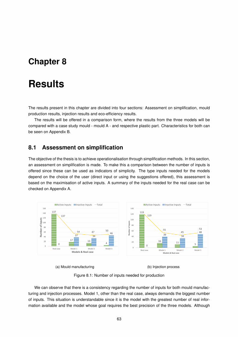
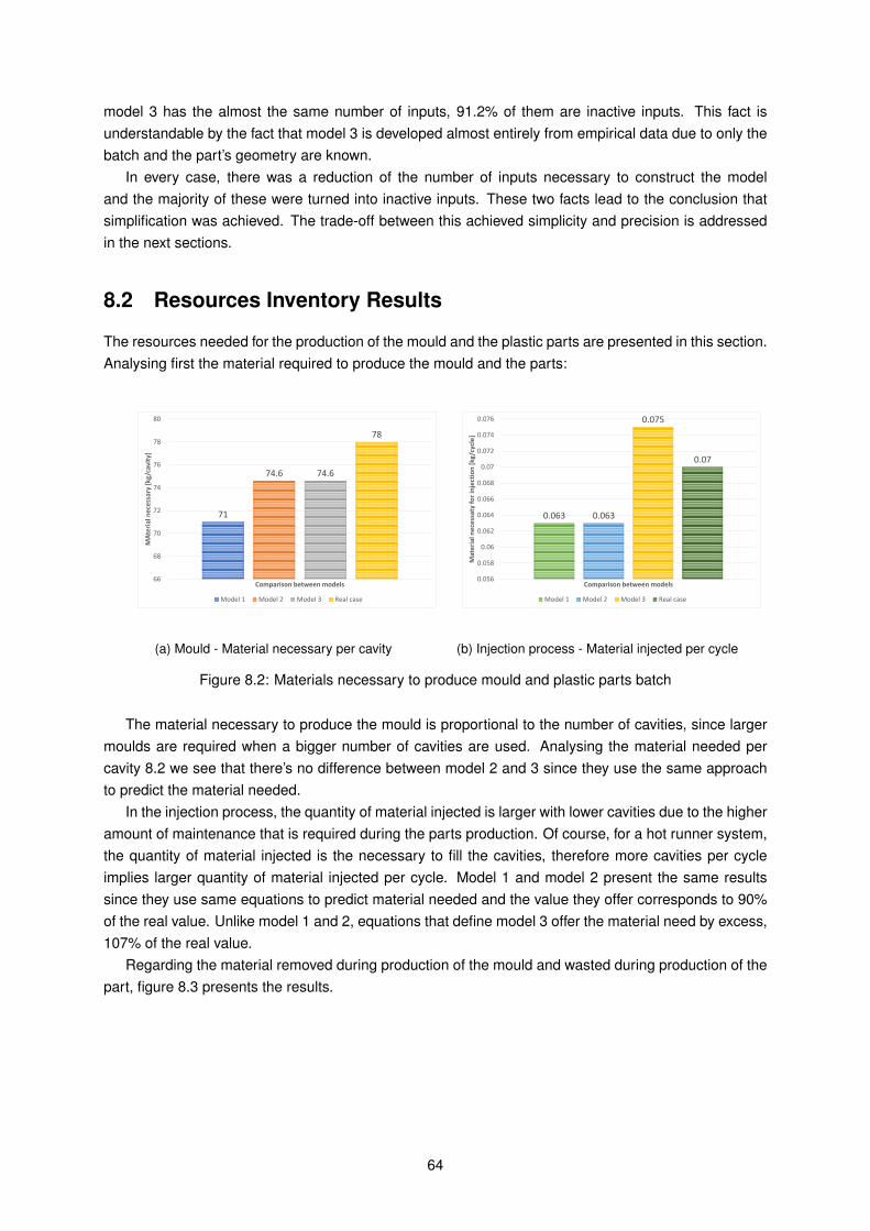
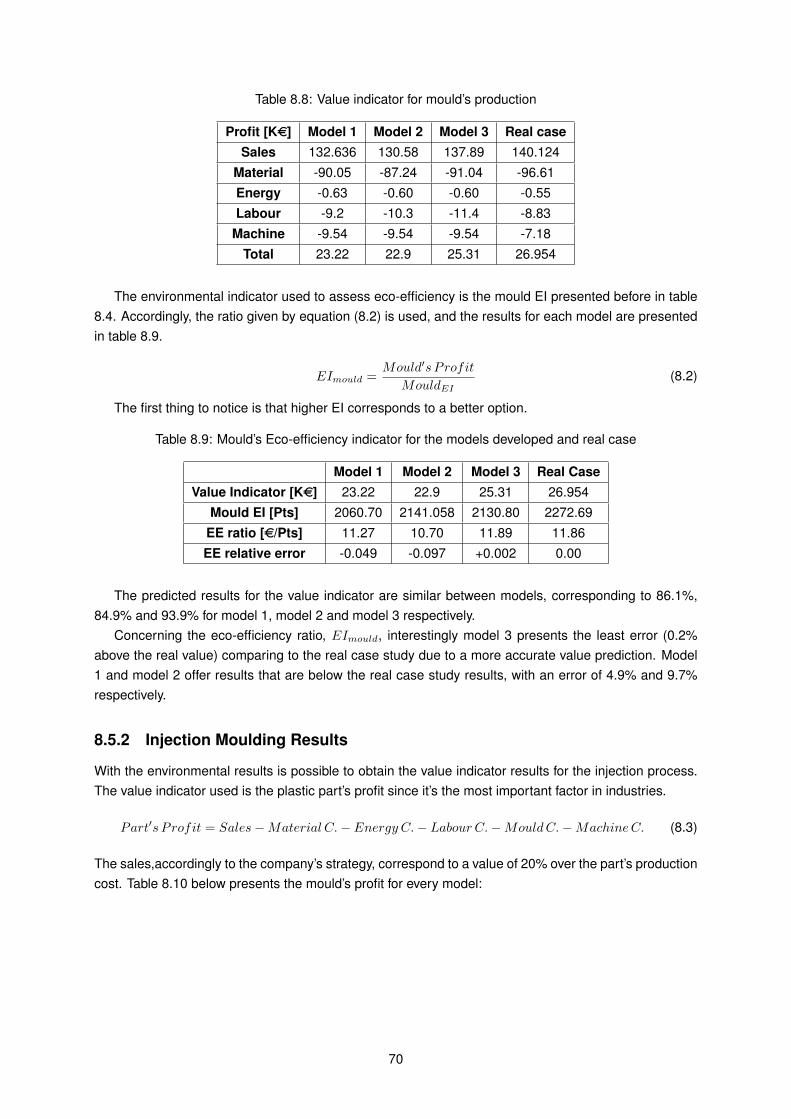
• Chapter 8 - Results. In this chapter individual results of each model are compared with one an-other. A assessment about if simplification was achieved is made together with its cost to accuracy.An analysis of the influence of few design aspects have over results is made.
• Chapter 9 - Conclusions and Future work. A final statement is made regarding the develop-ment of the proposed models and their results and some suggestions about this work’s futuredevelopments are offered.
3
4
Chapter 2
State of the Art
2.1 Eco-efficiency
2.1.1 Philosophy and principles behind eco-efficiency
Since the beginning of the industrial era, the corporate sphere has had an immense impact on theenvironment. In the 20th century, environmental movements started pointing out that there were en-vironmental costs associated with the manufacturing industries and in the at the end of the century,environmental problems became global in scale. An increasing global awareness of the threat posed byignoring environmental impacts gave birth to a new paradigm, which brought to centre stage the pursuitof a common ideal. In the industrial field, this new paradigm brought the appearance of a new philoso-phy where not only economic indicators were used to assess a business model but also environmentalindicators.
The first notion of eco-efficiency can be traced back to AM Freeman III and RH Haveman in the 70sas the concept of “environmental efficiency” [17].
In the 1990s, Schaltegger and Sturm [18] introduced eco-efficiency as a “business link to sus-tainable development”. In 1992, the concept of eco-efficiency was widely popularised in ChangingCourse (Schmidheiny 1992), a publication of the World Business Council for Sustainable Development(WBCSD) [19].
Since then, eco-efficiency has been accepted as a philosophy that intends to help businesses under-stand how the search for environmental improvements can yield economic benefits, thus showing howachieving both environmental and business goals can be compatible.
Being a relatively new concept, a standard definition of eco-efficiency does not exist, but several def-initions were proposed (see table 2.1) and although there are some differences between the definitionsshown, it’s possible to draw some similarities, they all address the need of creating more value and lessimpact. Thus, eco-efficiency can be seen as a broader manifestation of the concept of resource effi-ciency – minimising the resources used in the production of a unit of output – and resource productivity– the efficiency of economic actions in creating added value for the use of resources.
5
Table 2.1: Several definitions of eco-efficiency.[1][2][3]
Entity responsible for the definition EE definitionOrganisation for Economic Cooperation and Development (OECD) ”the efficiency with which ecological resources are used to meet human needs”
ISO/DIS 14045”quantitative management tool that enables the consideration of life cycleenvironmental impacts of a product system alongside its product system valueto a stakeholder”
European Environment Agency (EEA)
”A concept and strategy enabling sufficient delinking of the ‘use of nature’from economic activity needed to meet human needs (welfare) to allow itto remain within carrying capacities, and to permit equitable access anduse of the environment by current and future generations”
From the various definitions that appeared the one provided by WBCSD is often referred in worksrelated to eco-efficiency, and it will be the one used in this work also. According to WBCSD, “eco-efficiency is achieved by the delivery of competitively-priced goods and services that satisfy humanneeds and bring quality of life, while progressively reducing ecological impacts and resource intensitythroughout the life-cycle, to a level at least in line with the Earth’s estimated carrying capacity” [20].Eco-efficiency can be calculated using equation 2.1 [21].
(2.1)Eco− efficiency =Production or service value
Environmental Influence
In the business sphere, WBCSD affirms that to become more eco-efficient, a company should focuson well-known methods and strategies and as such, to help companies achieve a better eco-efficiency,proposed seven elements which may lead to improved eco-efficiency in business [20], [21], [5]. Theseseven principles are presented in table 2.2 where they were grouped accordingly with their function.
Table 2.2: Seven principles of eco-efficiency as stated by WBCSD.[4]
Function of the principle Eco-efficiency principle
Resource optimizationReduce material requirements
Reduce energy intensityReduce toxic dispersion
Increase of valueEnhance material recyclability
Maximize use of renewable resources
Reduction of environmental impactsExtend product durabilityIncrease service intensity
Even though the seven principles show in table 2.2 were proposed by WBCSD, they can be insertedin any of the definitions presented previously. They work on what is similar between them - the possibilityof obtaining more value using less material and energy inputs with the emissions reduction, and theyshow that eco-efficiency can be an integral part of the strategy that any organisation has [20].
2.1.2 Eco-efficiency indicators
Taking into consideration the vast number of definitions for eco-efficiency and the fact that they sharethe same core ideas, we can affirm that eco-efficiency concept is well-established. Nonetheless, lookingat the equation that quantifies eco-efficiency we notice that the concepts of value and environmental aregeneric and vague, leading to the possibility of different interpretations. Thus the necessity of havingappropriate metrics that allow a better orientation is essential [22].
The necessity of quantifying eco-efficiency in order to gather quantitative and qualitative informationfor making decisions gave birth to EE indicators. Indicators are defined as parameter or reference for aparameter and serve the purpose of assessing the progress of a company [13].
6
In order to ensure indicators are relevant, accurate and scientifically supportable, WBCSD presentedeight characteristics that indicators should have [14]:
(i) “Be relevant and meaningful with respect to protecting the environment and human health and/orimproving the quality of life”
(ii) “Inform decision making to improve the performance of the organization”
(iii) “Recognize the inherent diversity of business”
(iv) “Support benchmarking and monitoring over time”
(v) “Be clearly defined, measurable, transparent and verifiable”
(vi) “Be understandable and meaningful to identified stakeholders”
(vii) “Be based on an overall evaluation of a company’s operations, products and services, especiallyfocusing on all those areas that are of direct management control”
(viii) “Recognize relevant and meaningful issues related to upstream and downstream aspects of acompany’s activities”
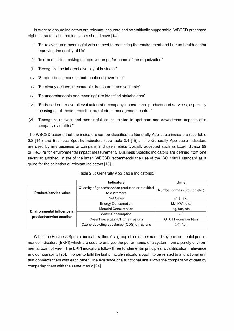
The WBCSD asserts that the indicators can be classified as Generally Applicable indicators (see table2.3 [14]) and Business Specific indicators (see table 2.4 [15]). The Generally Applicable indicatorsare used by any business or company and use metrics typically accepted such as Eco-Indicator 99or ReCiPe for environmental impact measurement. Business Specific indicators are defined from onesector to another. In the of the latter, WBCSD recommends the use of the ISO 14031 standard as aguide for the selection of relevant indicators [13].
Table 2.3: Generally Applicable Indicators[5]
Indicators Units
Product/service valueQuantity of goods/services produced or provided
Within the Business Specific indicators, there’s a group of indicators named key environmental perfor-mance indicators (EKPI) which are used to analyse the performance of a system from a purely environ-mental point of view. The EKPI indicators follow three fundamental principles: quantification, relevanceand comparability [23]. In order to fulfil the last principle indicators ought to be related to a functional unitthat connects them with each other. The existence of a functional unit allows the comparison of data bycomparing them with the same metric [24].
So, if different Generally Applicable indicators have the same units they will be comparable to eachother, while the business specific indicators are defined according to company necessities, becomingmostly significant to the company. The EKPI are comparable to each other when they have the samefunctional unit.
2.1.3 Use of eco-efficiency in industries
Although the majority of the concepts analysed until now refer to the business sector,eco-efficiency is atool capable of reaching broader horizons. For example, adopting eco-efficiency at the economy-widestage can be done at several levels of the economy – micro, macro and regional [22]. At this stage,governments may use eco-efficiency indicators as targets that correspond to environmental goals, anduse them to develop regional or national strategies.
In 2003, Basque government applied the concept of eco-efficiency to four economic sectors – trans-port, industry, energy and residential, in order to study the relationship between certain economic activ-ities and environmental pressures [7].
At the macro level, the Government of Japan utilised eco-efficiency in the areas of CO2 emissions,final energy consumption and the amount of municipal solid waste generated, to draw comparisonsbetween other OECD countries [7]. Eco-efficiency was expressed in terms of environmental load perunit of economic activity (e.g. CO2 per GDP), which shows a different way of presenting equation 2.1,and was used as a standard in assessing the performance of countries.
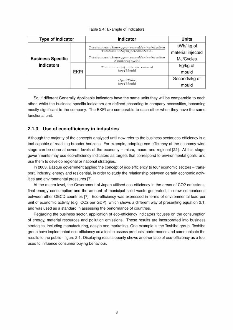
Regarding the business sector, application of eco-efficiency indicators focuses on the consumptionof energy, material resources and pollution emissions. These results are incorporated into businessstrategies, including manufacturing, design and marketing. One example is the Toshiba group. Toshibagroup have implemented eco-efficiency as a tool to assess products’ performance and communicate theresults to the public - figure 2.1. Displaying results openly shows another face of eco-efficiency as a toolused to influence consumer buying behaviour.
8
Figure 2.1: Eco-efficiency at the Toshiba Group[7]
Eco-efficiency’s universality can be proved by the multitude of areas where it has been used. Scien-tific papers which have eco-efficiency as base can be found is areas like electricity production [25], fruitproduction [26], steel industry [27], biocomposites [28], logistics networks [29].
The examples described above show that although being an extensive philosophy, eco-efficiencypresents a major drawback. Defining eco-efficiency as the ratio between value and environmental impact2.1, leads to the necessity of finding these two quantities for any given system. This characterizationprocess can be quite complex due to the necessity of knowing the economic (if the value was definedas such) and environmental impacts of a system in its entire life cycle [30].
This drawback leads to the conclusion that finding a way to turn EE operational, i.e. turn the formula-tion of EE and its indicators simpler, would be tremendously useful to companies, organisations or anyother entity who wishes to apply this philosophy in a regular way.
2.2 The injection mould
In this section some background information about injection moulds will be given.The mould importance for the injection process is substantial, not only it’s the most relevant tool for
the process, but it also represents an important part of the cost of the entire operation. Its weight onfinal cost is so relevant that a great deal of time is given to design, operation and maintenance of it [31].
The principal function of a mould is the production of quality parts in the shortest cycle time possible,and accordingly to A.Cunha [32] it must be capable of: define the volume with the shape to produce,ensuring the dimensional reproducibility, cycle by cycle; allow the fill of this volume with melted polymer;facilitate the cooling of the polymer and promote the extraction of the part.
Though moulds are usually made of steel or aluminium [33], the use of steel is more frequent due toits higher resistance that leads to a higher lifetime, meaning that, depending on the production volume,the initial investment can be returned. In the case of low production volumes, mould’s life length can besacrificed, therefore aluminium is often the choice due to his lower initial cost.
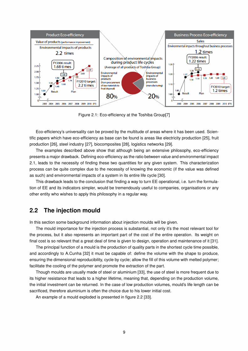
An example of a mould exploded is presented in figure 2.2 [33].
9
Figure 2.2: Exploded representation of a typical mould [8]
The typical injection mould consists of several plates, namely: cavity and core plates, forming thepart cavity, support plates, retaining plate and ejector pin plate. These are generally made out of steelby machining, usually milling, and their dimensions are function of the number of cavities and the size ofthe parts being manufactured.
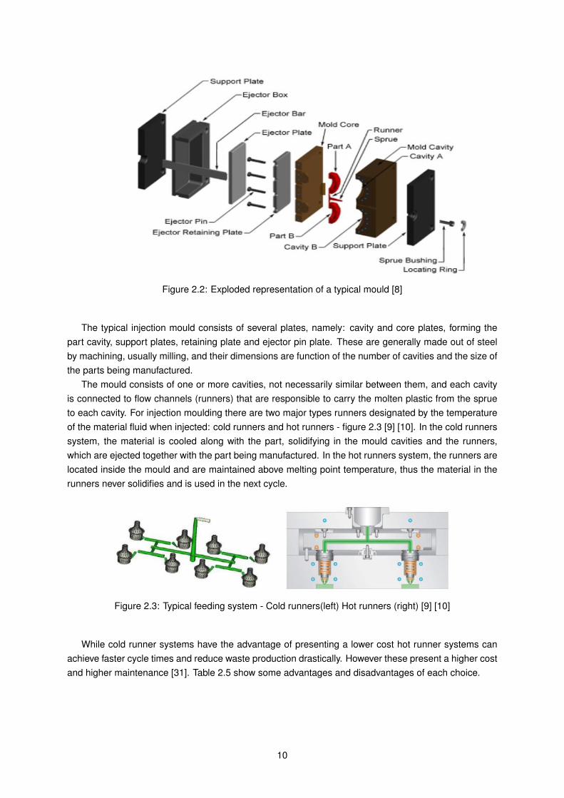
The mould consists of one or more cavities, not necessarily similar between them, and each cavityis connected to flow channels (runners) that are responsible to carry the molten plastic from the sprueto each cavity. For injection moulding there are two major types runners designated by the temperatureof the material fluid when injected: cold runners and hot runners - figure 2.3 [9] [10]. In the cold runnerssystem, the material is cooled along with the part, solidifying in the mould cavities and the runners,which are ejected together with the part being manufactured. In the hot runners system, the runners arelocated inside the mould and are maintained above melting point temperature, thus the material in therunners never solidifies and is used in the next cycle.
Figure 2.3: Typical feeding system - Cold runners(left) Hot runners (right) [9] [10]
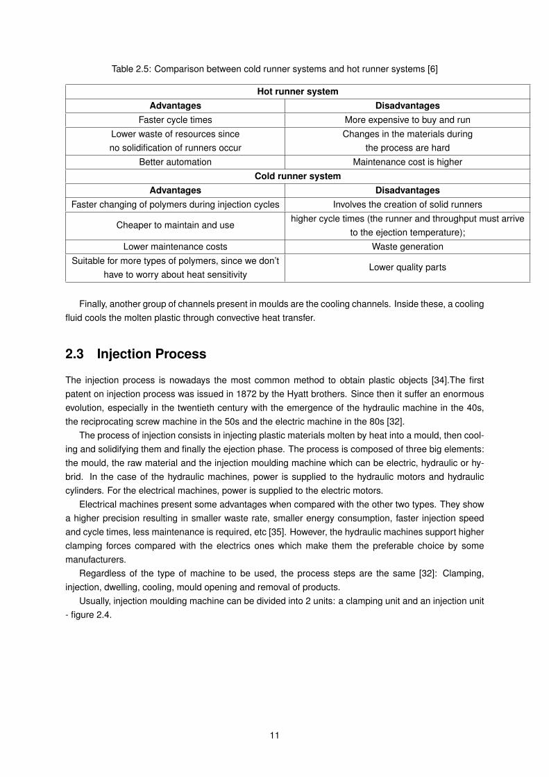
While cold runner systems have the advantage of presenting a lower cost hot runner systems canachieve faster cycle times and reduce waste production drastically. However these present a higher costand higher maintenance [31]. Table 2.5 show some advantages and disadvantages of each choice.
10
Table 2.5: Comparison between cold runner systems and hot runner systems [6]
Hot runner systemAdvantages Disadvantages
Faster cycle times More expensive to buy and runLower waste of resources sinceno solidification of runners occur
Changes in the materials duringthe process are hard
Better automation Maintenance cost is higherCold runner system
Advantages DisadvantagesFaster changing of polymers during injection cycles Involves the creation of solid runners
Cheaper to maintain and usehigher cycle times (the runner and throughput must arrive
to the ejection temperature);Lower maintenance costs Waste generation
Suitable for more types of polymers, since we don’thave to worry about heat sensitivity
Lower quality parts
Finally, another group of channels present in moulds are the cooling channels. Inside these, a coolingfluid cools the molten plastic through convective heat transfer.
2.3 Injection Process
The injection process is nowadays the most common method to obtain plastic objects [34].The firstpatent on injection process was issued in 1872 by the Hyatt brothers. Since then it suffer an enormousevolution, especially in the twentieth century with the emergence of the hydraulic machine in the 40s,the reciprocating screw machine in the 50s and the electric machine in the 80s [32].
The process of injection consists in injecting plastic materials molten by heat into a mould, then cool-ing and solidifying them and finally the ejection phase. The process is composed of three big elements:the mould, the raw material and the injection moulding machine which can be electric, hydraulic or hy-brid. In the case of the hydraulic machines, power is supplied to the hydraulic motors and hydrauliccylinders. For the electrical machines, power is supplied to the electric motors.
Electrical machines present some advantages when compared with the other two types. They showa higher precision resulting in smaller waste rate, smaller energy consumption, faster injection speedand cycle times, less maintenance is required, etc [35]. However, the hydraulic machines support higherclamping forces compared with the electrics ones which make them the preferable choice by somemanufacturers.
Regardless of the type of machine to be used, the process steps are the same [32]: Clamping,injection, dwelling, cooling, mould opening and removal of products.
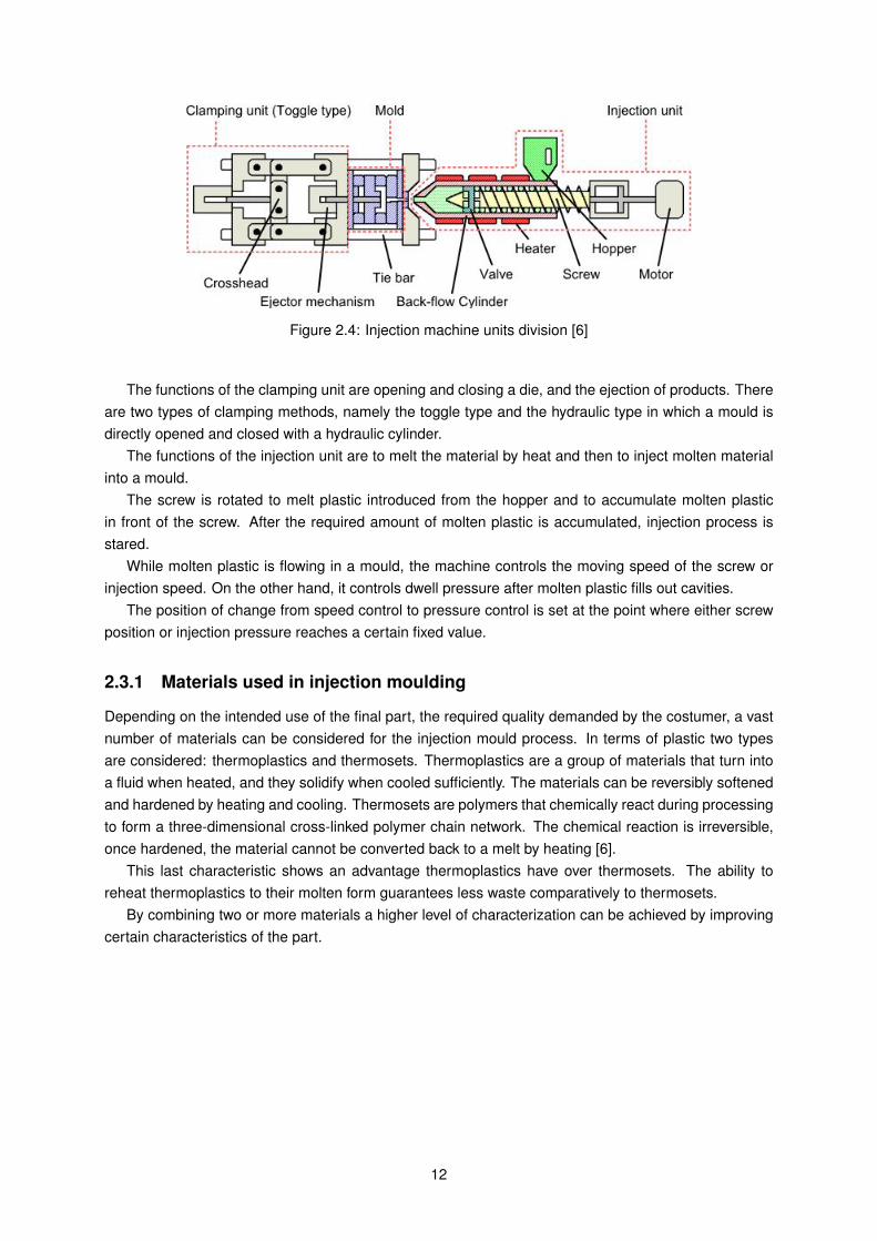
Usually, injection moulding machine can be divided into 2 units: a clamping unit and an injection unit- figure 2.4.
11
Figure 2.4: Injection machine units division [6]
The functions of the clamping unit are opening and closing a die, and the ejection of products. Thereare two types of clamping methods, namely the toggle type and the hydraulic type in which a mould isdirectly opened and closed with a hydraulic cylinder.
The functions of the injection unit are to melt the material by heat and then to inject molten materialinto a mould.
The screw is rotated to melt plastic introduced from the hopper and to accumulate molten plasticin front of the screw. After the required amount of molten plastic is accumulated, injection process isstared.
While molten plastic is flowing in a mould, the machine controls the moving speed of the screw orinjection speed. On the other hand, it controls dwell pressure after molten plastic fills out cavities.
The position of change from speed control to pressure control is set at the point where either screwposition or injection pressure reaches a certain fixed value.
2.3.1 Materials used in injection moulding
Depending on the intended use of the final part, the required quality demanded by the costumer, a vastnumber of materials can be considered for the injection mould process. In terms of plastic two typesare considered: thermoplastics and thermosets. Thermoplastics are a group of materials that turn intoa fluid when heated, and they solidify when cooled sufficiently. The materials can be reversibly softenedand hardened by heating and cooling. Thermosets are polymers that chemically react during processingto form a three-dimensional cross-linked polymer chain network. The chemical reaction is irreversible,once hardened, the material cannot be converted back to a melt by heating [6].
This last characteristic shows an advantage thermoplastics have over thermosets. The ability toreheat thermoplastics to their molten form guarantees less waste comparatively to thermosets.
By combining two or more materials a higher level of characterization can be achieved by improvingcertain characteristics of the part.
12
Chapter 3
Operationalisation of Eco-efficiencyModels
In the last chapter, a brief summary about the state of art of Eco-Efficiency was made. It was shownthat its use goes beyond a mere ”green” ideology but it can bring numerous economic benefits. It wasalso shown that one of the main obstacles to its use resides in the fact that a prior study to the systembeing analysed is indispensable, based on the fact that every characteristic that influences economic orenvironmental impacts must be accounted. The complexity of gathering the necessary data needed forthe use of eco-efficiency varies accordingly to the complexity of the system that we wish to evaluate, butit’s often time-consuming and arduous.
It’s exactly in this time-consuming and arduous work this dissertation will focus. Methods about howto turn the use of Eco-efficiency practical will be proposed together with results that validate the choicesproposed.
3.1 Operationalisation and simplification concepts
Although operationalisation and simplification can be interpreted as similar concepts, they carry differentmeanings in this work.
Operationalisation should be seen as the act of making something practical, of easy usage. On theother hand, the use of simplification should be considered as a mean to reach that operationalisation.
Regarding eco-efficiency, as shown in the previous chapter, its use carries some difficulties, namely,the elevated number of inputs that feed an eco-efficiency model and the arduous work needed to obtainthem. These obstacles, make the use of eco-efficiency non-practical i.e. non-operational for regular use.
This transformation of a non-operational model towards an operational one is the main objective ofthe dissertation and will be accomplished by simplifying methods.
Through expediting calculations and the use of empirical data to turn variable inputs into constants,an practical method can be achieved. These simplifications does not mean lack of rigour but a way tomake the use of Eco-efficiency more practical, i.e. operational.
Summing up, operationalisation should be achieved by means of simplifying processes and choices.This idea of simplification of methods will be shown in this dissertation through three different mod-
els representing three different scenarios connected to distinct moments of the use of eco-efficiencyin mould and injection industries 3.1. These three stages were chosen by identifying key distinct mo-ments within the manufacturing process. And thereafter those stages were validated by interviewing themanufacturing directors of a relevant company.
13
Although each one of these models will be presented individually in the chapters that follow this one,a brief description shall be presented in the next paragraphs so the reader has a succinct idea of thembefore approaching those chapters.
E.E. non operational on regular
basis
Simplification method
Operational E.E. method
Model 1
Model 2
Model 3 Op
era
tio
nal
izat
ion
m
od
els
Figure 3.1: Thesis overview - Problem, method and goal
3.2 Simplification models and exclusive model objectives
Before presenting any type of model a brief explanation about the existing system of the mould andplastic injection industry must be provided. Commonly the group of mould manufacturing and plasticinjection industries can be divided into three types:
• exclusive mould manufacturers - This kind of situation refers to those companies that solelymanufacture moulds for the injection industry. In this type of companies, the plastic injection pro-cesses are non-existent.
• exclusive plastic injection manufacturers - This kind of situation refers to those companies thatsolely act on the plastic injection process. In this type of companies, the mould is acquired from athird party. Mould manufacturing is non-existent.
• hybrid manufacturers - This kind of situation refers to a mix of the previous two types. In this typeof company the majority of the processes are exercised ”indoors”, from the mould creation to thefinal piece obtained from plastic injection.
Along this work only the two first types of manufacturers will be addressed, due to the fact that the lastone - hybrid manufacturers - can be seen as the pairing of the first two entities: mould manufacturerstogether with plastic injection manufacturers, being the characteristics of this last type the sum of thecharacteristics of the first two types.
After having defined the scope of the model (mould manufacturing and plastic injection processes),a more precise location in time for the models is needed.
In order to identify the steps, representing the temporal area of action, necessary to the manufac-turing process several visits to a manufacturing company were done and, together with the productionmanagers, a set of phases were identified. Along with this work, the system in study was defined by aset of phases, namely, ”Project development”, ”Negotiation phase”, ”Start of mould production”, ”End of
14
mould production”, ”Start of injection process”, and finally ”end of injection process”. This temporal flowis represented in figure 3.2.
Project Development
Negotiation Phase
Start of Mold Production
End of Mold Production
Start of Injection process
End of injection Process
Figure 3.2: Temporal universe of the system
The phases present above are defined as follows:
• Project development - First phase of the process. This is the phase where an idea for a newproject is born. It can be seen as a very early design stage, where the only few aspects aredefined. In this phase, the costumers are the stakeholders, not the company.
• Negotiation Phase - This is the phase where manufacturers negotiate product characteristics(price included) with potential costumers. It’s in this phase, that the final concept for the productbeing manufactured appears and where some manufacturing choices are made due to the client’sdemands. It requires knowledge about capabilities of the manufacturing assets.
• Start of mould production - First phase of the mould manufacturing process. It’s the phase wheredecisions about mould production are made. In this phase the answer to the question ”How will wemanufacture this mould?” is given. Namely, it’s in this stage that machines and other assets areallocated to the project.
• End of mould production - Last phase of the mould manufacturing process. In this phase theproduct manufacturer is able to analyse the project that ended.
• Start of injection process - Similar to the first stage of mould production, in this phase the finaldecisions about injection process are made. In this phase the answer to the question ”How will wemanufacture this product?” is given.
• End of injection process - Last phase of the process. It’s in this last phase that the manufacturercan review all the process and gather information that allows future improvements in the system.
3.2.1 Simplification models - First approach
The definitions presented above help contextualise the simplification models being developed and, al-though each one of them is described in an individual chapter, a brief description of them and thescenario they intend to represent is given:
The first model (model 1) presented in this work, is related to the selection of manufacturing pro-cesses for the mould manufacturing procedure. It arises in order to address the need of studying andpossibly improving the choice of the manufacturing process, and thus, it implies a good precision re-garding the results, meaning low error when comparing to the actual, non-simplified process.
15
The second model (model 2) presented in this work, is related to the negotiation phase of the process.It arises from the need of having real-time estimates of results, namely costs and environmental impacts.It’s expected that the results generated in this model, lack in terms of precision when in comparison withthe previous model.
The third and last model (model 3) presented in this dissertation, is related to an initial design phase.It emerges as a method of providing designers or any other entity that desires it so, a way of estimateresults when little is known about the processes needed to achieve the final product. Thanks to this lackof accurate data about the processes, this third model is expected to present the least accurate results.
3.2.2 Exclusive model objectives
One other aspect common to the three models that is necessary to introduce is the concept of .Recalling that the objective of the thesis is to develop operational models for the use of eco-efficiency,
leads to the conclusion that this also ought to be the main objective for each of the models developed.Although the models have the same main objective, they differ from each other because, as statedbefore, each one of them represents a different scenario. Due to this difference, a new set of objectivesarises, objectives that intend to represent the necessities that each scenario presents. For example,while the second model requires that a certain input should be easily edited by the user that same inputin any other model can be set as a fixed value, outside the immediate control of the user.
Due to this exclusivity of the models regarding some objectives and in order to differentiate themfrom the main one (to develop an operational model for the use of eco-efficiency), it was settled thatthese set of objectives will be known as exclusive model goals.
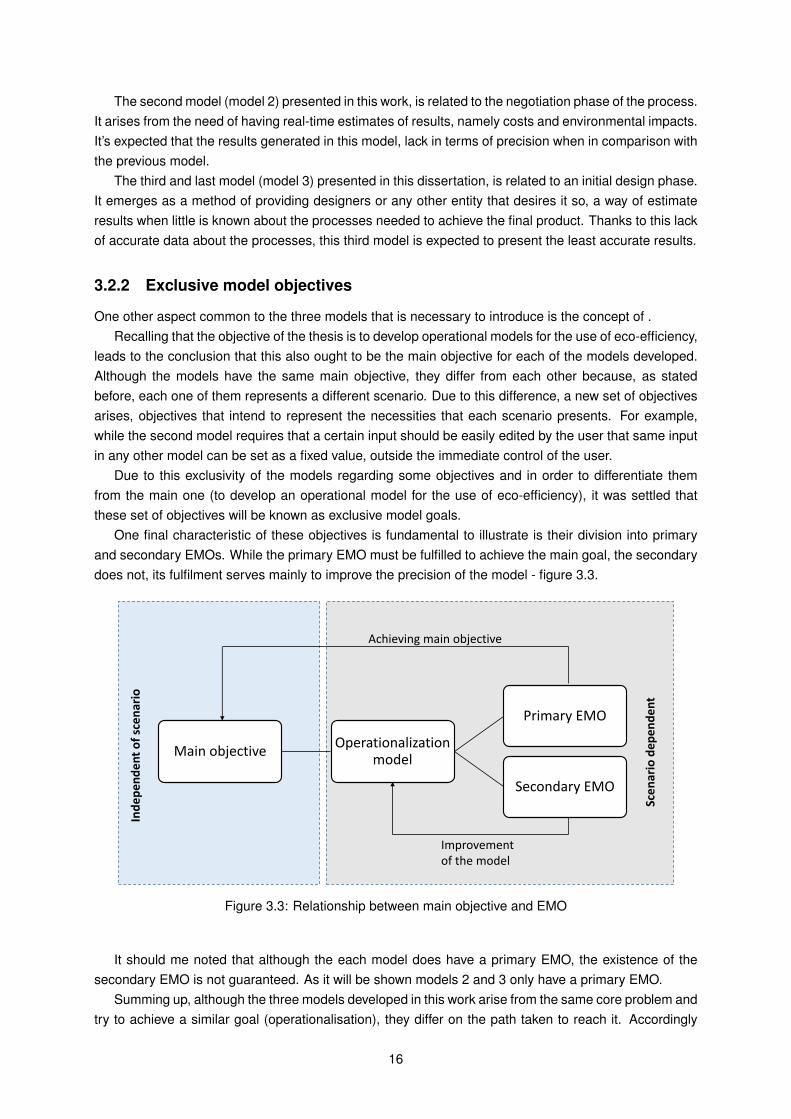
One final characteristic of these objectives is fundamental to illustrate is their division into primaryand secondary EMOs. While the primary EMO must be fulfilled to achieve the main goal, the secondarydoes not, its fulfilment serves mainly to improve the precision of the model - figure 3.3.
Main objectiveOperationalization
model
Primary EMO
Secondary EMO
Sce
nar
io d
epen
den
t
Ind
ep
end
en
t o
f sc
en
ario
Achieving main objective
Improvement of the model
Figure 3.3: Relationship between main objective and EMO
It should me noted that although the each model does have a primary EMO, the existence of thesecondary EMO is not guaranteed. As it will be shown models 2 and 3 only have a primary EMO.
Summing up, although the three models developed in this work arise from the same core problem andtry to achieve a similar goal (operationalisation), they differ on the path taken to reach it. Accordingly
16
to the model’s stage of operation, distinctive mechanisms will be used to simplify the ”real”, originalmodel.3.1
3.2.3 Type of inputs
One last aspect it’s important to explain is the existing division of inputs that feed the models. Theseinputs were divided into two groups: active inputs and inactive inputs. Active inputs are those that mustbe loaded by the user every time the model is used. This gives some degree of freedom to the user.
Inactive inputs are fixed (constant value) inputs. These must be loaded previously to the use of themodel and are used together with active inputs to predict results. Loading the models with inactive inputscan be a time-consuming task, but has the advantage of only being done the first time the model is usedor when something major changes in the manufacturing company - figure 3.4.
Active inputs
Inactive inputs
Model’s equations Model’s output
Inp
uts
div
isio
n
Inputs overview
Pre-fixed values
Variable values
Figure 3.4: Inputs division used in this work
3.2.4 Models Validation
There are 5 moulds available to do the mould model’s validation and the respective 5 parts to do theplastic part’s validation. Moulds are named from Mould A to Mould E and the respective parts, Part A,Part B, etc. In the validation section, one of the moulds will be chosen randomly to perform the validation.
In order to model the system, data was gathered by doing several visits to a mould and injectionmanufacturing site. Thereafter, the model was validated using data from that same company. This canbe seen as an ”overfitting” feature and possible a drawback in the model. Of course, using the samemethodology for different systems should be done carefully, and one should expect larger precisionerrors according to how different that same system is from a mould and injecction system.
Before ending the chapter, one last note should be delivered. It should be pointed out that thesemodels do not intent to be a closed system whose users cannot manipulate. These models should beseen as guidebooks, a set of simplification rules/suggestions created in order to achieve the intendedgoals.
In the next chapter, the first of the three models will be presented in a more detailed way.
17
18
Chapter 4
Operationalisation Model – Processselection model
This chapter will address the first operationalisation model, thus it will be essential to detail it – whatscenario it represents, what its goals are and who will benefit from its use. For a better understanding ofthe model developed, the overall methodology is presented in this chapter, followed by the model itself.
Finally, this operational model must be validated. To do it so, it will be used a real case study from amould manufacturing and plastic injection company.
4.1 Model characterization
Accordingly to what was presented in the previous chapter, the model being described was designed toreduce the problem identified in the introductory chapter - elevated complexity of making eco-efficiencystudies in the mould and plastic injection industries. But, of course, this is true to all three models presentin this thesis. What differentiate them is the scenario they represent.
The first model developed arises from the necessity of having real-time data that would serve as abase to make process decisions allowing the educated choices about what path to take to achieve thedesired results.
In relation to to the different types of industries presented in the previous chapter, it must be notedthat although the model acts in both exclusive mould manufacturers and exclusive plastic injection man-ufacturers its role differs depending on the type of manufacturer.
For exclusive mould manufacturers, and remembering figure 4.2, it can be noted that using the modelat ”Start of Mould Production” gives the manufacturer data that allows selecting the better path for themanufacturing of the mould and using the model in ”Star of Injection Process” provides data aboutinjection process. The usefulness of such data for exclusive mould manufacturers is diverse. It can beseen as adding value to the service provided if we consider that this data can be delivered to clients withthe mould.
Regarding the other type of industry - plastic injection manufacturers - the utility of the model relieson a similar explanation. For exclusive plastic injection manufacturers, the model is able to provide anestimation or more precise data about the injection process if estimation inputs or real ones are used(obtain from a post production stage), respectively.
Using the same model at the end of production, feeding it with real results instead of predicted ones,gives more precise results and therefore can be used to study the processes and gather relevant datato improve the model and future choices.
19
The capabilities described in the last paragraphs can be translated into EMO (see chapter 3.2.2).Accordingly, the primary EMO is the capability of predicting economic, energetic and eco-efficiencyindicators for the moulds to be manufactured and for the plastic injection process. The secondary EMOis the ability to feed a database of characteristics of the processes. This allows a better understandingof the processes by comparing the manufactured mould and plastic piece’s process characteristics withothers previously made, giving the model a continuous improvement capability.
Thus it can be concluded that, and in consequence of the definition of primary and secondary EMO,the completion of the primary EMO is mandatory to achieve the objective of the thesis, since the dis-sertation objective demands a simplified model for eco-efficiency, while the completion of the secondaryEMO is optional. The secondary EMO allows the user to store the results of every mould a plastic pieceproduced allowing a better understanding of the processes by comparing the manufactured mould’s pro-cess characteristics with others previously made, and as such, it provides the model with a continuousimprovement capability. See figure 4.1
Exclusive model
objectives
Dissertation objective
Operationalization
Primary EMO’s
Results prediction
Secondary EMO’s
Results database
Figure 4.1: Main objective and exclusive model objectives
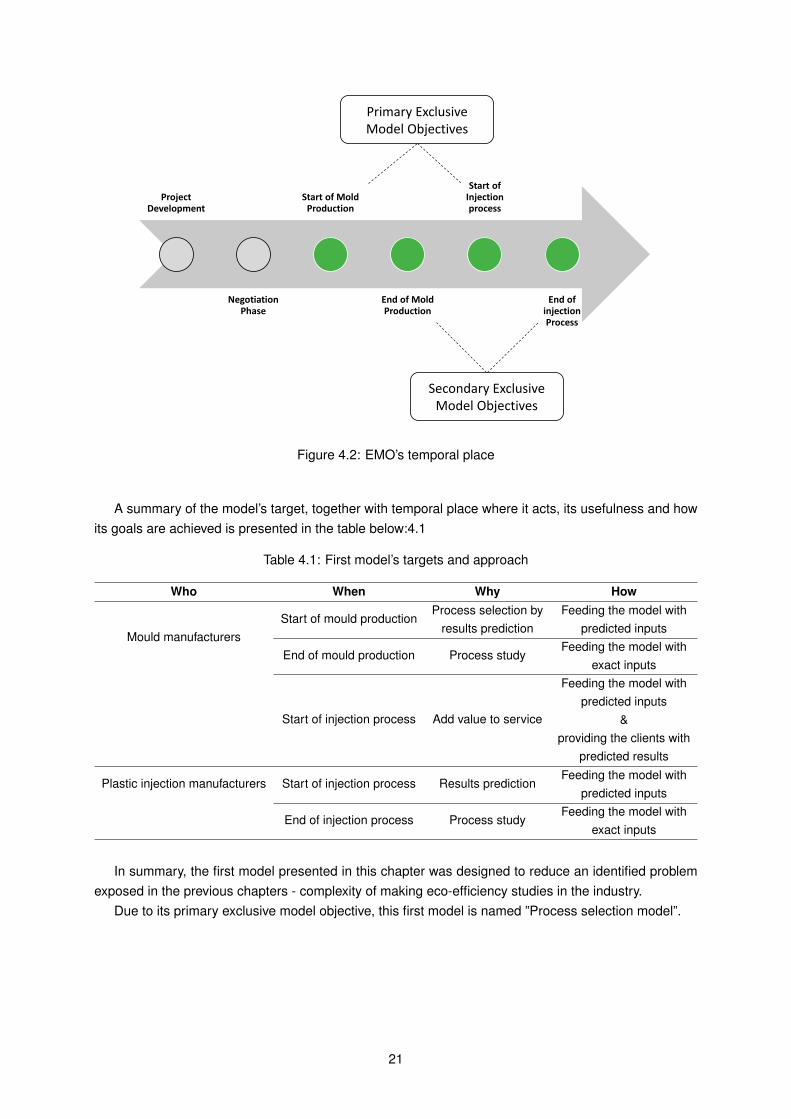
One of the main differences between these two exclusive model objectives resides at the differenttime stage where they act (figure 4.2). While the secondary one, in order to fulfil the requirement ofcreating a database, demands input values with minor errors and therefore known values, which can beobtained in a post-production stage, the first one doesn’t do it so. In order to fulfil this primary objective(capability of predicting economic, energetic and eco-efficiency indicators), predictions about processcharacteristics can be seen as acceptable inputs.
20
Project Development
Negotiation Phase
Start of Mold Production
End of Mold Production
Start of Injection process
End of injection Process
Primary Exclusive Model Objectives
Secondary Exclusive Model Objectives
Figure 4.2: EMO’s temporal place
A summary of the model’s target, together with temporal place where it acts, its usefulness and howits goals are achieved is presented in the table below:4.1
Table 4.1: First model’s targets and approach
Who When Why How
Mould manufacturersStart of mould production
Process selection byresults prediction
Feeding the model withpredicted inputs
End of mould production Process studyFeeding the model with
exact inputs
Start of injection process Add value to service
Feeding the model withpredicted inputs
&providing the clients with
predicted results
Plastic injection manufacturers Start of injection process Results predictionFeeding the model with
predicted inputs
End of injection process Process studyFeeding the model with
exact inputs
In summary, the first model presented in this chapter was designed to reduce an identified problemexposed in the previous chapters - complexity of making eco-efficiency studies in the industry.
Due to its primary exclusive model objective, this first model is named ”Process selection model”.
21
4.2 Methodology
The general methodology applied will be presented in this section. Every main step applied in the modelwill be described.
Following the background provided in chapter 1, the first step is recognising and identifying the needto develop a model that fills the existing gap in the mould and injection industries regarding eco-efficiency.Having done this, the time and the model’s scenario of operation was defined. (See figure 4.3)
Project Development
Negotiation Phase
Start of Mould
Production
End of Mould
Production
Start of injection process
End of injection Process
Figure 4.3: First model’s time of operation. Primary EMO in green and secondary EMO in blue
After the goal was defined, the development of the model began with the division of the process intwo major groups: mould production and plastic injection process.
Following the previous step, a breakdown on the first major group started. A study was made todefine what manufacturing sub-groups compose the mould manufacturing process and for each group,what sub-processes are part of them. To achieve this, studies from previous works and several visitsto a hybrid company were done. This information gathering allowed to understand the place of severalvariables and achieve valid simplifications, whose objective is, as stated before, serve as backbone tooperationalisation of the model.
As the sub-processes were defined, the identification of the variables that compose those sub-processes was done, always having in mind the necessity of simplification. Thus variables with lowrelevance to cost or energetic impact were neglected.
Finally, the influence of several components and variables that compose an injection mould weremodelled.
Finished the mould manufacturing part of the model, the injection process part was created.In the same way of the mould creation process, the plastic injection process was considered as a
process composed by sub-processes, thus the first step in the model design was to establish allsub-processes and the inputs variables that are part of them, defining not only the process but also the partto be manufactured in terms of batch, type of machine, etc.
Having established the part dimensions and process data, it was possible to validate the model andpresent the results.
It’s important to notice that the goal of this model, as stated before, is to create a model that iscapable of operating in different companies, as such, two alternatives to inputs were created. The firstset of inputs that feed the model are inputs whose origin can be traced to data from previous studiesand different companies - empirical evidence. The second set of inputs, working as an alternative to thefirst set, are inputs related to the particular company using the model. These inputs need to be insertedin the system beforehand, but bring better precision to results.
Within these two sets of inputs, two subgroups were defined, active inputs and inactive inputs, thuscreating a division between inputs that need constant updates each time a new manufacturing processbegins and those inputs that need only to be changed when the company in question performs somestructural change in the way it performs.
To validate the model created a real case study was used - production of conventional steel mouldsand the injection of the respective plastic pieces. The results associated with this model are presentedin the chapter ”Results”, where different mould alternatives are analysed and compared.
22
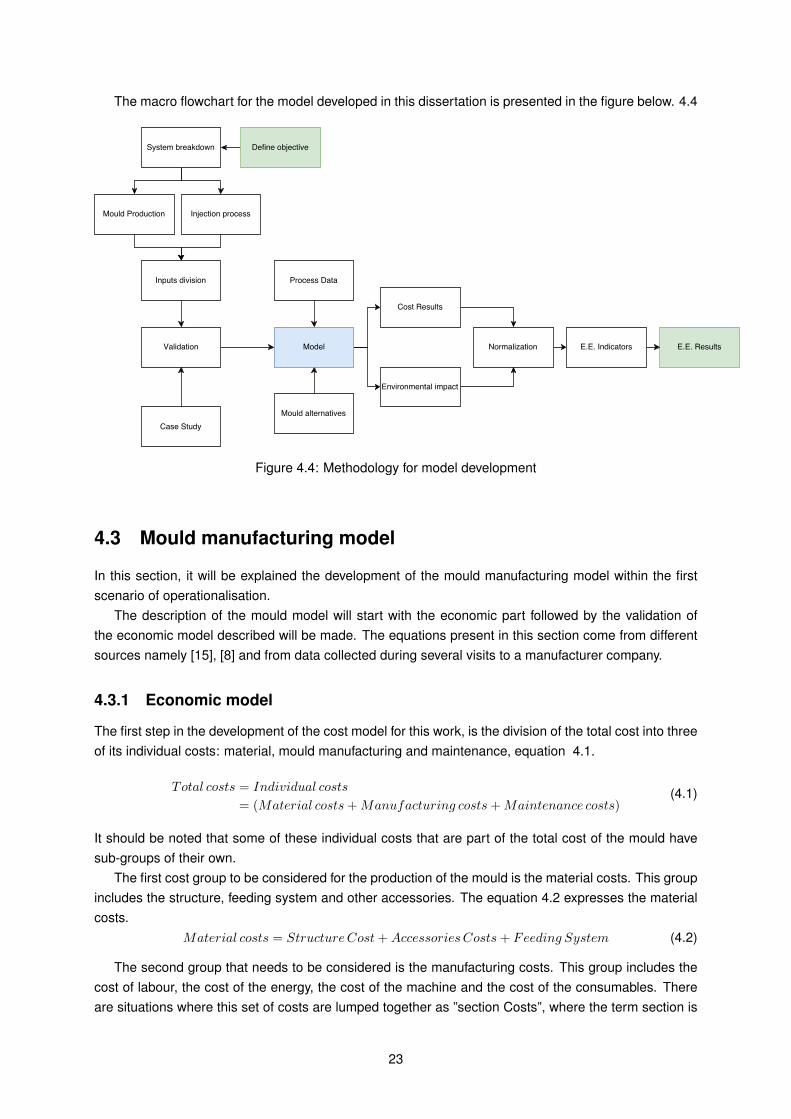
The macro flowchart for the model developed in this dissertation is presented in the figure below. 4.4
Figure 4.4: Methodology for model development
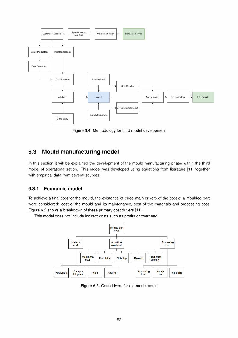
4.3 Mould manufacturing model
In this section, it will be explained the development of the mould manufacturing model within the firstscenario of operationalisation.
The description of the mould model will start with the economic part followed by the validation ofthe economic model described will be made. The equations present in this section come from differentsources namely [15], [8] and from data collected during several visits to a manufacturer company.
4.3.1 Economic model
The first step in the development of the cost model for this work, is the division of the total cost into threeof its individual costs: material, mould manufacturing and maintenance, equation 4.1.
It should be noted that some of these individual costs that are part of the total cost of the mould havesub-groups of their own.
The first cost group to be considered for the production of the mould is the material costs. This groupincludes the structure, feeding system and other accessories. The equation 4.2 expresses the materialcosts.
Material costs = StructureCost+AccessoriesCosts+ Feeding System (4.2)
The second group that needs to be considered is the manufacturing costs. This group includes thecost of labour, the cost of the energy, the cost of the machine and the cost of the consumables. Thereare situations where this set of costs are lumped together as ”section Costs”, where the term section is
23
connected to the type of manufacturing process being used. Equation 4.3 translates the manufacturingcosts.
Manufacturing costs = Labour cost+ Energy cost+Machine cost+ consumable costs (4.3)
The last element that integrates cost of producing a mould is maintenance cost of the machines andit’s calculated using equation 4.4
Maintenance costs = maintenance allocated%×∑
(Mainmachine cost+ tool cost) (4.4)
An overview of the model is show in figure 4.5:
Materials & Accessories
Structure
Accessories
Feeding system
Manufacturing
Labour
Energy
Machine & Consumables
Maintenance
Investment
Main machine
Cost
Tool Costs
Figure 4.5: Economic model major groups overview
Remembering that the model presented in this work is connected with the idea of simplificationof methods, a detailed analysis of each sub-group, where the simplifications made are explained, isnecessary.
Materials cost
• Structure costs
Starting with the analysis of structure costs, the first step and simplification is to identify the relevantelements that make the structure. These are: clamp plates, mould plates, ejector plates, and ejector set.The next simplification made in ”structure costs” is the transformation of the costs of each component,where common heat treatments and polishing process are included, listed before from active inputs toinactive inputs. To do this, a table relating the dimensions of mould plates (height, width, thickness) andthe cost of those components should be created beforehand and fed to the model, this gives the user allstructure costs from only 3 active inputs for plate. The creation of this table can be done using data frommoulds already built. Although this can be a time-consuming work, it only has to be done once, savingtime in the long run.
In the situation where the desired dimensions are not present in this cost table, the desired cost canbe calculated using the set equation shown in table 4.2 where h,w,t represent respectively height, width
24
and thickness expressed in millimetres. These equations were determined applying a fuzzy algorithm todata from previously made moulds and it was considered that the structure is made from a generic steelwhose cost is around 4.5e per kg. In a very simple way, fuzzy is a logical method that finds approximaterelations between inputs and respective outputs [36].
Table 4.2: Cost [euros] equations, deduced using a fuzzy algorithm
Structure Element Cost EquationClamp Plates 0.733h× 0.113w × 0.154t
Mould Plates 0.631h× 0.201w × 0.168t
Ejector Plates 0.722h× 0.107w × 0.171t
Ejector Set 0.801h× 0.098w × 0.101t
• Accessories
Regarding the accessories costs, the users have two options to enter them into the model, the first one isby direct input and the second one is by selecting from a predefined list of the most common accessoriesand respective costs, the ones that are part of the mould being manufactured. This second option arisesfrom the fact that it may be difficult to introduce specific values for the accessories. Therefore, constantcost values are suggested. These come from average values from empirical data. Table 4.3 shows thesuggested accessories cost values.
Table 4.3: Suggested cost per accessory for common accessories
Finally, the user must provide dimensions for cavity inserts and the material price they are made of.In the case, the user doesn’t provide the material, this is assumed as a martensitic stainless steel with afixed cost of 7.9e/kg. In case this information is uploaded in the model it must be inserted together withthe material density [kg/mm3] and its price [e/kg].
• Feeding System
In this case, there are some options the user must define to calculate the cost: number of nozzles,existence or not of hot runners, type of manifold bloc and cost of the injection controller - equation 4.5.
(4.5)Feeding system costs=Number of nozzles×nozzle cost+Distribution bloc cost+controller cost
The cost of the nozzles should be inserted in the model as an inactive input, by studying the company’sroutines and fixing an average value in the model. The same situation for the controller. In the case ofthe cost of the manifold bloc, it depends greatly on the type of bloc used, so a list of common types usedby the company must be fed to the model, together with their cost, as a set of inactive inputs.
Manufacturing costs
The determination of manufacturing costs starts by defining what processes are part of a mould man-ufacturing process. These are: milling (conventional and CNC), wire and penetration EDM, grinding,laser, turning (conventional + CNC) , CAD, CAM and small manual processes.
• Labour Costs
25
Labour costs are define as the sum of cost of labour internal to the company with the subcontractsmade.
Labour costs associated with a specific process is given by equation 4.6 :
(4.6)Labour costsinternal =Man/hour cost× process time
And the cost of worker per hour is given by equation 4.7:
(4.7)Man/hour cost =Monthly wage× shifts× 14× taxesnumber days year ∗ working hours day
To simplify the calculation of labour costs a few assumptions were made, these are consideredinactive inputs. First of all, the worker’s occupation rate is considered 100%, taxes over wages of 23%,the number of working days in a year is considered to be 240 and a working day is considered to have8 hours. Regarding the cost of the subcontracts, this input is asked to the user as a percentage of theinternal labour cost, thus being an active input.
The default value is 10% of the total production cost, this was suggested by the engineer responsiblefor the mould production.
• Energetic Costs
The energetic cost depends on several factors namely, on the machine, on the processing time and onenergy cost. This relationship between factors is translated by equation 4.8
(4.8)Energy cost[e] = Energy unit cost[e/kWh]× Energy[kWh]
There are two ways to introduce the energy variable into the model, the first is to previously take severalmeasurements directly from the machines and use the average energetic value from those measure-ments, the second one is by using the 60% of the apparent power of the connected machine. Thissecond option can be justified by the analysis of the energetic map of several moulds, where the ma-chine works on average at 60% of its apparent power. Both of these options are fed by inactive inputs,in the first case the energy consumed by the machine and in the second case the apparent power of themachine.
The energy unity cost input, since it is tabled by EDP for industries - Energias de Portugal and majorchanges occur seldom, it’s considered an inactive input and its value was fixed at 0.062 [e/kWh] [37].
• Machine Costs
The cost of the machine is dependent on the machine cost per hour and on the processing time. Thecost is given by equation 4.9
(4.9)Machine cost =Machine cost per hour [e/h]× Processing time [h]
The machine cost per hour can be determined by using equation 4.10, where I is the acquisition cost ofthe equipment, r is the fixed interest rate, that was fixed as 10% and n is the depreciation time.
(4.10)Machine cost per hour[e] = I×(1−(1+r)−n)r × 1
working days per year×working hours per day
The acquisition time is considered an inactive input, therefore it is necessary to create a databasecontaining the acquisition cost for each machine before the use of the model.
In order to simplify the entry of inputs, the depreciation time n was considered to be 8 years [38].
• Consumables Costs
26
The consumable group is composed of the machine’s tools used in the manufacturing of the mould andby the cutting fluids that are needed for some processes. Starting by the cutting fluids, the cost of thefluid is given by equation 4.11
(4.11)Ccf = Ptime × CFcons × CFc
where Ccf represents the cost of cutting fluid (e), Ptime represents the process time (h), CFcons thecutting fluid consumption (dm3/h) and CFc the cutting fluid cost (e/dm3). To simplify the model thecutting fluid consumption and cutting fluid cost were set as constant value (inactive input). Althoughthe cutting fluid consumption parameter changes accordingly with machining characteristics [39], it wasobserved that the difference between processes was negligible, thus this value was set as 0.0012dm3/h.The fluid cost was set as 8 e/h. One final thing that should be noted in regards to cutting fluid costs isthat in the case of the EDM processes, the costs associated with the fluid are inserted in the tool costgroup.
Finally, respecting the tools costs, equation 4.12 is used to determine the cost:
simplification is rather difficult since each machine uses different types of tools and each tool presentsdifferences in the wear rate. It is suitable to emphasize that the mould material has an important effecton the tool’s life and only steel moulds were studied, thus to reach a conclusion about tooling costs twocompanies were analysed - table 4.4
Table 4.4: Tooling cost from 2 different companies for steel moulds
Company Anual Cost of tools [e] Hours/year machines e/hCompany 1 94866 32712 2.9Company 2 74750 28750 2.6
To simplify the tooling cost an average value was chosen, therefore the tooling cost per hour was setas 2.75 e/h.
Maintenance costs
In the case of the maintenance costs, the main machine cost and consumables costs subgroups wereaddressed in the previous subsection and the maintenance investment is an active input of the model.
Complexity factor
After putting all the previous costs together it was noted that there was a gap between real cost andthe costs presented by the model. This was due to the fact that the complexity of the mould was notbeen taken into account. In order to solve this, a new active input was developed - complexity input, thatrepresents a constant value used to multiply by equation (4.1) giving the final cost of the mould.
Still regarding the complexity input, the model demands that the user selects one of three levels ofcomplexity for the mould being developed. The first level represents the simplest mould possible, whereneither the object being produced has a complex geometry nor the mould need to have some complexcinematic, like for example rotation. The second level represents a mould more complex than a com-plexity 1 mould, and is related to the manufacturing of objects with complex geometry, but where themould has simple linear movements. The third complexity level represents a mould developed to man-ufacture objects with complex geometries and non-linear movements. This non-linearity of movements
27
requires the existence of non-ordinary accessories in the mould, increasing its cost. Table 4.5 shows themultiplying factors for each complexity level. These were obtained together with the production managerof a company, by first defining the complexity of several moulds and then finding an average value foreach complexity level that reduced the gap between the model’s results and real results.
Table 4.5: Complexity Cost factors
Complexity Level 1 2 3Cost factor 1.00 1.05 1.10
4.3.2 Model Validation
In order to validate the simplified cost model, a real case study was used. This case study, and in orderto validate the complexity input, is composed by 2 different moulds. In order to fulfil the non-disclosureagreement, images of the mould will not be shown and the manufacturing company identity will not berevealed.
Table 4.6 presents the principal dimensions of the moulds used to validate the model.
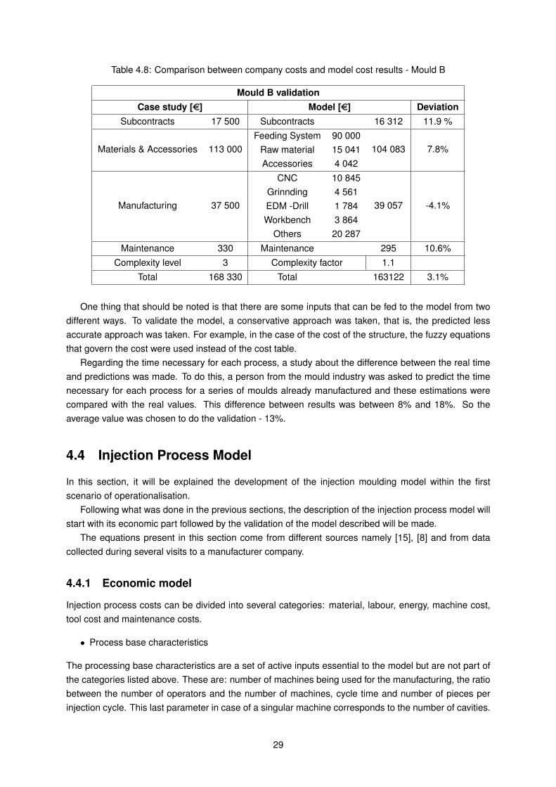
Tables 4.7 and 4.8 present the cost results for the case studies and the current model. A comparisonbetween both is also shown through the deviation between costs.
For mould E of complexity level 1, the deviation between the model and the case study is around2.3%. For mould B the deviation lies at 3.1%.
For each case presented, although the major deviation occurs in the subcontract values, the mostsignificant deviation takes place in the manufacturing group.
Table 4.7: Comparison between company costs and model cost results - Mould E
Mould E validationCase study [e] Model [e] Deviation
One thing that should be noted is that there are some inputs that can be fed to the model from twodifferent ways. To validate the model, a conservative approach was taken, that is, the predicted lessaccurate approach was taken. For example, in the case of the cost of the structure, the fuzzy equationsthat govern the cost were used instead of the cost table.
Regarding the time necessary for each process, a study about the difference between the real timeand predictions was made. To do this, a person from the mould industry was asked to predict the timenecessary for each process for a series of moulds already manufactured and these estimations werecompared with the real values. This difference between results was between 8% and 18%. So theaverage value was chosen to do the validation - 13%.
4.4 Injection Process Model
In this section, it will be explained the development of the injection moulding model within the firstscenario of operationalisation.
Following what was done in the previous sections, the description of the injection process model willstart with its economic part followed by the validation of the model described will be made.
The equations present in this section come from different sources namely [15], [8] and from datacollected during several visits to a manufacturer company.
4.4.1 Economic model
Injection process costs can be divided into several categories: material, labour, energy, machine cost,tool cost and maintenance costs.
• Process base characteristics
The processing base characteristics are a set of active inputs essential to the model but are not part ofthe categories listed above. These are: number of machines being used for the manufacturing, the ratiobetween the number of operators and the number of machines, cycle time and number of pieces perinjection cycle. This last parameter in case of a singular machine corresponds to the number of cavities.
29
In the case of multiple machines, if the cycle time is the same (as in the case of matching machines),this parameter corresponds to the sum of the cavities in all the machines. Finally, in the case of multipledifferent machines being used this parameter corresponds to the number of parts manufactured fromthe moment the first parts are done until the last machine finishes the first set of parts.
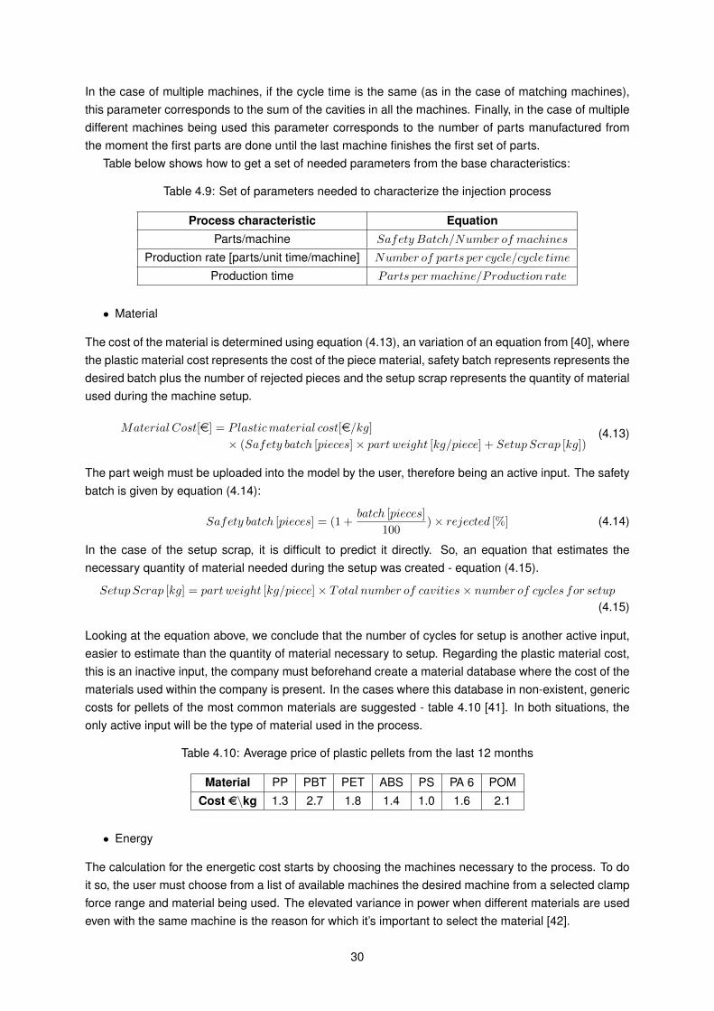
Table below shows how to get a set of needed parameters from the base characteristics:
Table 4.9: Set of parameters needed to characterize the injection process
Process characteristic EquationParts/machine Safety Batch/Number of machines
Production rate [parts/unit time/machine] Number of parts per cycle/cycle time
Production time Parts permachine/Production rate
• Material
The cost of the material is determined using equation (4.13), an variation of an equation from [40], wherethe plastic material cost represents the cost of the piece material, safety batch represents represents thedesired batch plus the number of rejected pieces and the setup scrap represents the quantity of materialused during the machine setup.
The part weigh must be uploaded into the model by the user, therefore being an active input. The safetybatch is given by equation (4.14):
(4.14)Safety batch [pieces] = (1 +batch [pieces]
100)× rejected [%]
In the case of the setup scrap, it is difficult to predict it directly. So, an equation that estimates thenecessary quantity of material needed during the setup was created - equation (4.15).
SetupScrap [kg] = partweight [kg/piece]× Total number of cavities× number of cycles for setup(4.15)
Looking at the equation above, we conclude that the number of cycles for setup is another active input,easier to estimate than the quantity of material necessary to setup. Regarding the plastic material cost,this is an inactive input, the company must beforehand create a material database where the cost of thematerials used within the company is present. In the cases where this database in non-existent, genericcosts for pellets of the most common materials are suggested - table 4.10 [41]. In both situations, theonly active input will be the type of material used in the process.
Table 4.10: Average price of plastic pellets from the last 12 months
Material PP PBT PET ABS PS PA 6 POMCost e\kg 1.3 2.7 1.8 1.4 1.0 1.6 2.1
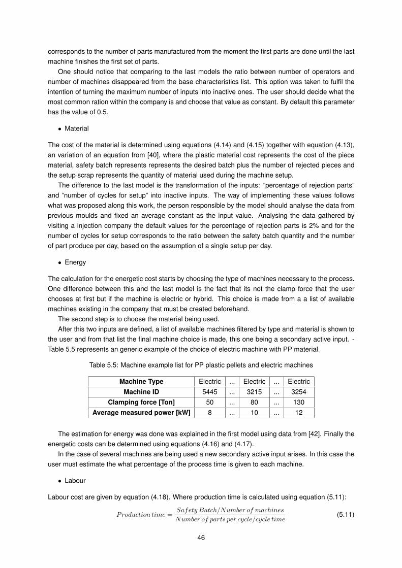
• Energy
The calculation for the energetic cost starts by choosing the machines necessary to the process. To doit so, the user must choose from a list of available machines the desired machine from a selected clampforce range and material being used. The elevated variance in power when different materials are usedeven with the same machine is the reason for which it’s important to select the material [42].
30
This machine list, that must be created beforehand accordingly with the company assets, includesfour types of entries per material: Identification of the machine, clamping force, average energy con-sumption, type (electric, hydraulic or hybrid).
The creation of this list is a time-consuming work since entails a series of measurements for eachmachine and for each material since material does influence the energetic input.
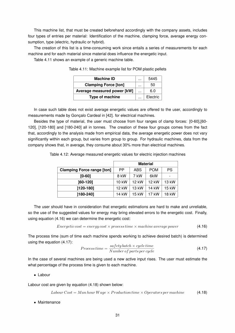
Table 4.11 shows an example of a generic machine table.
Table 4.11: Machine example list for POM plastic pellets
Machine ID ... 5445Clamping Force [ton] ... 50
Average measured power [kW] ... 6.0Type of machine ... Electric
In case such table does not exist average energetic values are offered to the user, accordingly tomeasurements made by Goncalo Cardeal in [42]. for electrical machines.
Besides the type of material, the user must choose from four ranges of clamp forces: [0-60],[60-120], [120-180] and [180-240] all in tonnes. The creation of these four groups comes from the factthat, accordingly to the analysis made from empirical data, the average energetic power does not varysignificantly within each group, but varies from group to group. For hydraulic machines, data from thecompany shows that, in average, they consume about 30% more than electrical machines.
Table 4.12: Average measured energetic values for electric injection machines
The user should have in consideration that energetic estimations are hard to make and unreliable,so the use of the suggested values for energy may bring elevated errors to the energetic cost. Finally,using equation (4.16) we can determine the energetic cost:
(4.16)Energetic cost = energy cost× process time×machine average power
The process time (sum of time each machine spends working to achieve desired batch) is determinedusing the equation (4.17):
(4.17)Process time =safety batch× cycle timeNumber of parts per cycle
In the case of several machines are being used a new active input rises. The user must estimate thewhat percentage of the process time is given to each machine.
• Labour
Labour cost are given by equation (4.18) shown below:
(4.18)Labour Cost =ManhourWage× Production time×Operators permachine
• Maintenance
31
Equation (4.19) is used to calculate the maintenance costs needed to produce the batch of parts for theclient:
(4.19)MaintenanceCost = Cost per intervention× number of interventions needed
(4.20)Number of interventions needed =Number of cycles to produce batch
Number of cycles between interventions
The number or cycles between interventions is defined by the company, therefore it’s considered aninactive input.
Of course, if the number of cycles needed to fulfil the batch requirement is lower that the number ofcycles between interventions the cost is zero.
• Tool
The mould is the main tool used in injection moulding process.The tooling cost is calculated thoughequation (4.9) and (4.10) where I in this case represents the total mould cost, r is the interest rate and nis the number of years defined to pay the investment.
Both interest rate and depreciation time were set as inactive inputs using the constants 10% and 10years respectively.
• Machine cost
To determine the machine cost an identical approach to what was described in the mould productionphase was followed. Equations 4.9 and 4.10 were used. Both interest rate and depreciation time wereset as inactive inputs using the constants 10% and 10 years respectively.
• Complexity factor
Similarly to the mould production phase, a complexity factor is needed to achieve better accuracy on theresults. It corresponds to a factor that will be used to multiply the final cost with it.
The complexity factor tries to fill gaps in the cost models created by complex part geometries. In thesame way, a three level complexity factor was introduced in mould manufacturing phase, an identicalthree level system is part of the injection process cost model.
Each level of complexity translates more complex part geometries, being level 1 associated withparts with simpler geometries and level 3 with parts with complex geometries.
The correct complexity level selection depends on the user’s skill and experience.With the help of an injection production manager, it was possible to analyse several injected parts
costs ans it was possible to create a table that presents the relation between complexity level andcomplexity factors - table 4.13.
Table 4.13: Complexity Cost factors for injection process
Complexity Level 1 2 3Cost factor 1.00 1.1 1.15
4.4.2 Model Validation
In the same way. it was done in the validation of the economic model of the mould manufacturingprocess, the validation presented next will be done resorting to two case studies. The use of two casestudies instead of one will allow assessing the validity of the complexity factor, for that one plastic partof complexity level 1 and another of complexity level 3 will be used.
32
For confidentiality reasons a total breakdown of the injection costs cannot be presented, but only thefinal cost per sector.
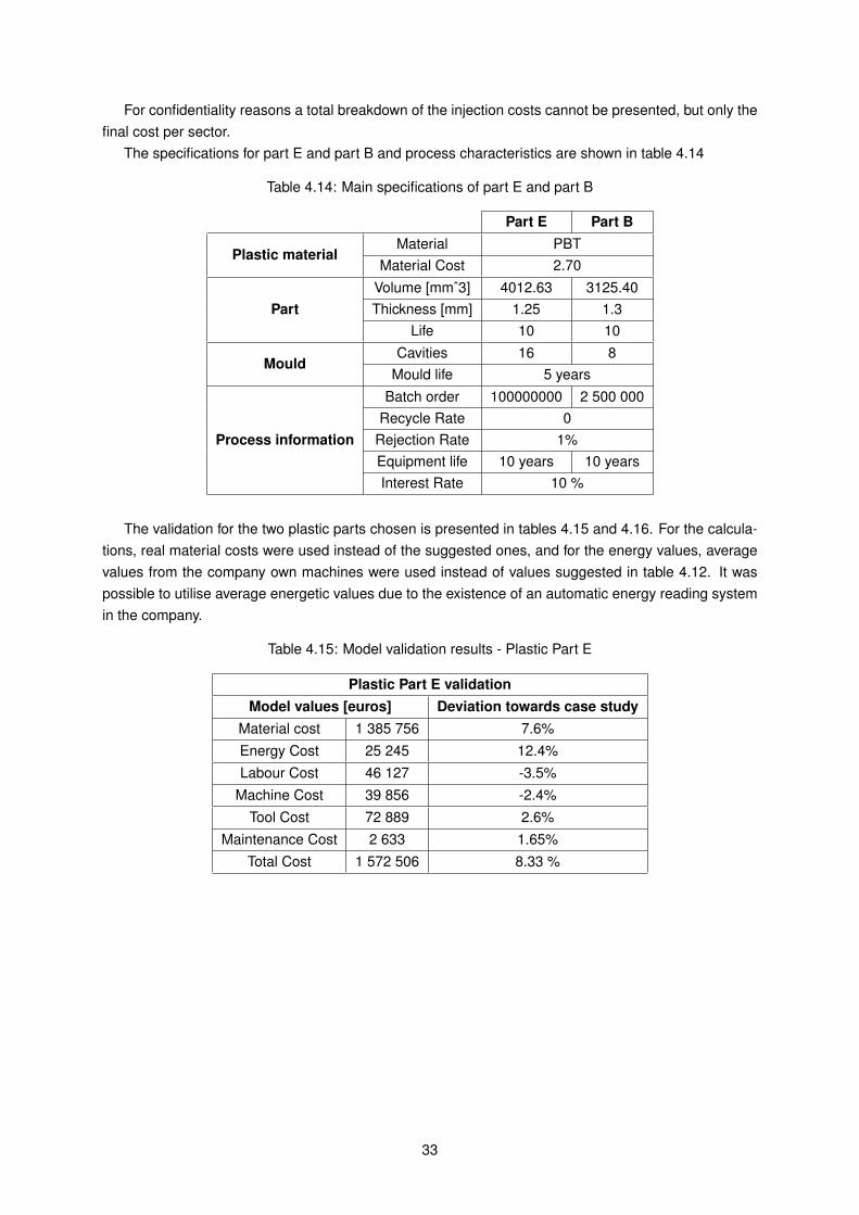
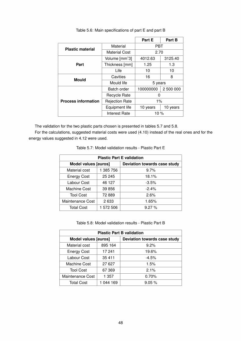
The specifications for part E and part B and process characteristics are shown in table 4.14
Table 4.14: Main specifications of part E and part B
Rejection Rate 1%Equipment life 10 years 10 yearsInterest Rate 10 %
The validation for the two plastic parts chosen is presented in tables 4.15 and 4.16. For the calcula-tions, real material costs were used instead of the suggested ones, and for the energy values, averagevalues from the company own machines were used instead of values suggested in table 4.12. It waspossible to utilise average energetic values due to the existence of an automatic energy reading systemin the company.
Table 4.15: Model validation results - Plastic Part E
Plastic Part E validationModel values [euros] Deviation towards case study
In the last chapter, it was presented the first of the three models covered in this dissertation. This chapterwill address the second model of operationalisation.
Following what was done in the last chapter, the methodology for this model will be offered, followedby the model itself.
Lastly, a validation of the model developed will be presented, resorting to a real case study from amould manufacturing and plastic injection company.
5.1 Negotiation Stage
Following the main concept of this dissertation and what was presented in the previous chapter, themodel described is inserted in the mould manufacturing and plastic injection processes. In this sub-chapter, it will be presented a more detailed description of the second model previously referred.
Using a similar approach with respect to the last model, a precise temporal location ought to bedefined.
The first step it’s important to take is to define the goals of this second model. As in the first model,the second model follows the macro objective of this dissertation, i.e, to provide a operational methodto the use of indicators of eco-efficiency by means of simplification of calculations and approaches, butit also has its own exclusive model objectives and, as in the previous model, these EMO were dividedinto two sets. The first and primary EMO is to provide estimations of results (once again, economic andenvironmental) giving negotiation flexibility to the manufacturers. The secondary EMO has a pedagogicaspect. By continuously dealing with costumers manufacturers will possibly learn costumers’ commonwishes. Learning what costumers generally want will provide information that can be used to improvethe model (see figure 5.1).
One practical example of the secondary EMO is the manufacturers understanding of the desire ofa new plastic material after several costumers inquire about the cost of making their product in thishypothetical material. With this new information, the model can be updated with data of this desiredmaterial.
35
Exclusive model
objectives
Dissertation objective
Operationalization
Primary EMO’s
Results prediction
Secondary EMO’s
Understanding what costumers
want
Figure 5.1: Main objective and exclusive model objectives for the second model
Taking the model presented in the previous chapter as base of comparison, it can be noticed thatthe distinction between primary and secondary EMO can be harder to make, thus a more detailedexplanation is needed.
From the primary EMO - to predict results in both economic and environmental spectres, obtainingat the same time negotiation flexibility - should result a set of data destined to the manufacturers. Thedata derived from the model, when this one’s used with the primary EMO in mind, should provide themanufacturers real-time weighted economic and environmental results, so they can be used to achievegreater flexibility in the negotiation aspect. For example, while negotiation with a potential client the initialproposal made by the manufacturer can be rejected by the client. The use of real-time results providedby the model allows an immediate counter-proposal by changing some parameters in the initial model(type of material, for example).
From the secondary EMO - obtaining information about what clients want - unlike the primary EMO,the data resulting from its use is destined to both manufacturers and client. The resultant data derivedfrom the model, when this one is used with the secondary objective in mind, targets not only the man-ufacturers, as referred before but also the clients. The manufacturers benefit from this information byupdating the model being used with new aspects. This is especially useful for example in the explorationof a new foreign market where what is assumed as common sense might not be so at the new market.
On the other hand, clients benefit from this by results related to what the costumer really wants.
36
Manufacturers Clients
Secondary Exclusive Model Objectives
Primary Exclusive Model Objectives
Figure 5.2: Exclusive objectives targets
It must be noted that in both cases, using the results achieved through the use of the model toreach an agreement, should be done carefully since these carry precision errors due to simplificationprocesses and inputs derived from estimations. Although the gap between real results and the outputsprovided by the model, these can be used as a first assessment of the model.
Using the set of phases presented previously in figure 3.2, the time stage where the two exclusivemodel objectives act can be shown.
Unlike the previous model where the exclusive model objectives acted in different time stages, inthis model the EMO act at the same place in time - Negotiation phase (see figure 5.3). Both of themrequire input values that feed a model based on key process characteristics considered essential in anegotiation table, as it will be seen further ahead.
Project Development
Negotiation Phase
Start of Mold Production
End of Mold Production
Star of Injection process
End of injection Process
Primary Exclusive Model Objectives
Secondary Exclusive Model Objectives
Figure 5.3: EMO’s temporal place
37
The intention of this second model is to provide an asset to both types of industrial schemes pre-sented in chapter 2 - mould manufacturers and plastic injection manufacturers. As such, and accordinglyto the EMOs presented before, the utility of the principal EMO is quickly understandable as it providesdata about the manufacturing process, allowing its manipulation and better understanding of how aspecific input influences the final results.
In the case of the exclusive mould manufacturers, the model is directed to mould production, allow-ing a negotiation based on initially estimated results. The models, can also provide estimations aboutinjection process, in this case, it contributes by adding value to the service provided since it can offer theclient that information as well.
For exclusive plastic injection the utility relies on the same explanation from above, except the resultsare directed to the production of plastic object.
A summary of the target company and is presented in the table 5.1 below:
Table 5.1: Second model’s applicable universe
Who When Why How
Mould manufacturers&
Plastic injecction manufacturers
Negotiation phaseResults prediction
Feeding the model withpredicted inputs
Add value to service
Feeding the model withpredicted inputs
&Providing the clients with
predicted results
Clients characterization
Learning what clients ingeneral want
&Updating the model with
those requirements
In summary, the second model presented in this chapter was designed to reduce an identified prob-lem exposed in the previous chapters - complexity of making eco-efficiency studies in the industry.
In this section, the stage where the model is to be directed was identified and explained, accordinglyto the exclusive objective defined.
Due to its area of acting, this second model will be referred as ”Negotiation Stage Model”.
5.2 Methodology
The general methodology applied will be presented in this section. Every main step present in the modelwill be described.
Following up the summary presented in chapter 1, the first step of the model’s development is rec-ognizing the existing gap in the industry regarding the use of eco-efficiency.
The next step is to define the area and time of operation(see figure 4.3).After the goals were defined, the development of the model began with the division of the process
into two production areas: mould and injection process.For each group, the identification of a set of characteristics (inputs) essential to a negotiation phase
was made. This division was possible by interviewing production managers connected to each area ofproduction.
38
Following the previous step, a breakdown of the first major group was done. It was defined whatmanufacturing sub-processes compose the mould manufacturing process by studying previous worksand by doing several visits to a hybrid company.
As the sub-processes were identified, the recognition of the variables that compose those sub-processes was done, and those with small influence in the final result were dropped.
This information gathering allowed to connect the previously identified essential inputs with otherprocess characteristics in order to create a model.
Finished the mould manufacturing part of the model, the injection process part was built. This wasdone in a similar manner with the exception of the identification of sub-processes, due to the fact thatplastic injection process was not considered as a process composed by sub-processes.
Having established the part dimensions and process data, it was possible to validate the model andpresent the results.
In an identical manner, regarding the first model, two alternatives to inputs were created. The firstset of inputs that feed the model, are inputs whose origin can be traced to data from previous studiesand companies - empirical data. The second set of inputs, working as an alternative to the first set, areinputs related to the specific company using the tool. Within this second set of inputs two subgroupswere once again defined, structural inputs and recurrent inputs.
To validate the model created a real case study was used - production of conventional steel mouldsand the injection of the respective plastic pieces. The results associated with this model are presentedin the chapter ”Results”, where different mould alternatives are analysed and compared.
The macro flowchart for the model developed in this dissertation is presented in the figure 5.4 below.
Figure 5.4: Methodology for second model development
5.3 Mould manufacturing model
In this section, it will be explained the development of the economic model of the mould manufacturingphase within the second model of operationalisation.
39
The description of the mould model will start with the identification of key parameters, then equationsthat describe the economic part follow and in the end the validation of the economic model describedwill be made.
The first step in the negotiation model is the identification of a set of useful inputs that manufacturerswould need to manipulate in real time during negotiations. To do this a series of visits to a manufactur-ing company was made together with several meetings with the director of the production from mouldmanufacturing area. From these meetings, key negotiation inputs were obtained. In the case of themould manufacturing process, these are: number of cavities, mould material, complexity, part height,part projected area and process time for each process - figure 5.5.
Of course, if these inputs can be modified at real time at the will of the user, then this fact makesthem active inputs by definition.
Although this mould model tries to take as active inputs only the parameters enumerated above,other active inputs are necessary to model the system. In order to differentiate the key negotiationinputs from the other active inputs, a new nomenclature was created for this model - primary activeinputs and secondary active inputs. Primary active inputs are those identified by production managersas essential to a negotiation meeting. Secondary active inputs are those that although must be uploadin real time were not identified as essential.
5.3.1 Economic model
Using the same equations [8] [15] and group cost breakdown that was used at the first model, the totalcost is divided into tree groups: material costs, manufacturing costs, and maintenance costs.
Materials cost
• Structure costs
40
In a similar way to what was done in the first model, the first step and simplification is to identify therelevant elements that compose the structure. Minor elements are neglected due to their low weight inthe final cost of the structure. As in the first model these are: clamp plates, mould plates, ejector plates,and ejector set. The cost is given by equation (5.1):
(5.1)StructureCost[e] =∑Plates cost[e] +Material and surface treatments cost[e]
Regarding the structure dimensions, it as assumed, after comparing dimensions from 6 differentmoulds, that the plates have the same dimensions between each other. Plates dimensions are given byequations (5.3) and (5.4), where where ncavitieslength and ncavitieswidth are the number of cavities acrossthe length and width dimensions [11].
Lmould = Lcavity · ncavitieslength · 1.33 (5.3)
Wmould =Wcavity · ncavitieswidth · 1.33 (5.4)
Of course, the manufacturer must define beforehand the minimum dimensions required by the injec-tion machine and use them in case the estimate dimensions are lower than that value.
Figure shows an example of a mould with four cavities with length and width of 8cm, thus the platesdimensions are 21.28cm by 21.28cm
Figure 5.6: Example of the size relation between plates and plastic part projected area
Finally, the treatments costs for each plate are fixed as 2% of the plate total cost given by equation(5.2).
• Accessories
Unlike the last model where users could enter accessories directly, in this case, in order to keep fulfilthe initial choice of having only the key negotiation inputs as active, the user must select the neededaccessories from a predefined list. Once again, the cost of the accessories come from average valuesfrom previous moulds manufactured within the company. In the case this list doesn’t exist the valuespresented before in Table 4.3 are suggested.
Another set of material cost is necessary to include is the cavity and core sets. This set is composedby: Cavity, Core, Cavity inserts and Core inserts. Since the cost of these elements are dependent ontheir size which is not an active input, an approximation was made. It was noted that in several cases
41
studied the sum of the volume of cavity and core sets corresponded to an average value of 6% of thevolume of the cavity plate, thus this value is used to define their whole volume. It was also assumedthat the material is Martensitic Stainless Steel with an average price of 7.9 e/kg and density 7.78 g/cm3.The cost can be determined by:∑
The way to determine the feeding system cost is identical to what was used in the first model - equation(4.5). Again, the cost of the nozzles should be inserted in the model as an inactive input, by studyingthe company’s routines and inserting an average value in the model. The same situation happens forthe controller. In the case of the cost of the manifold bloc, it depends greatly on the type of bloc used,so a list of common types used by the company must be fed to the model, together with their cost, as aset of inactive inputs.
Regarding the number of injection nozzles, it must be inserted by the user, thus being a secondaryactive input.
Manufacturing cost
Once again the cost of the manufacturing processes starts by defining what processes are part of amould manufacturing process. These are: milling (conventional and CNC), wire and penetration EDM,grinding, laser, turning (conventional + CNC) , CAD, CAM and small manual processes.
• Labour costs
Labour costs were defined as the sum of the cost of labour internal to the company with the subcontractsnecessaries. In this model the cost of subcontracts is an secondary active input, that must be defined bythe user accordingly with the project being negotiated. This input is asked as a percentage of the totalproduction cost.
By default is assumed that subcontracts correspond to 10% of the total production cost, as wassuggested by the manufacturing company visited to gather the necessary data.
For a specific manufacturing process the labour cost is given by equation (5.6):
(5.6)Labour costs = (Monthly wage× shifts× 14× taxesnumber days year ∗ working hours day
)× process time
Every input with the exception of the process time are inactive inputs that must be implemented accord-ingly with the company’s reality. Nonetheless, suggested values to those inputs are given: taxes overwages are fixed at 23%, number of working days in a year is considered to be 240 and a working day isconsidered to have 8 hours.
• Energy costs
The energetic cost depends on several factors including, type of machine, on the processing time andon energy cost. Energy cost can be determined using equation (5.7)
:
(5.7)Energy cost[e] =∑
(Energy unit cost[e/kWh]× Energy[kWh])
where the right side of the equation (5.7) represents the energetic cost of all machines.
• Machine costs
42
The cost of the machine is dependent on the machine cost per hour and on the processing time. Thecost is given by equation (5.8) that appears from merging equations (4.9) and (4.10):
(5.8)Machine cost = (I × (1− (1 + r)−n)
r× 1
working days per year × working hours per day)[e/h]
× Processing time [h]
In equation (5.8), I is the acquisition cost of the equipment, r is the fixed interest rate, that was fixed as10% and n is the depreciation time.
The acquisition time is considered an inactive input, therefore it is necessary to create a list of everymachine available, containing the its acquisition cost, prior to the use of the model.
In order to simplify the entry of inputs, the depreciation time n was considered to be 8 years [38].
• Consumables
Accordingly to what was proposed in the first model, the consumable group is composed by the ma-chine’s tools used in the manufacturing of the mould and by the cutting fluids that are needed for someprocesses. Consumables cost is given by equation (5.9), where Ccf [e] represents the cost of the cuttingfluid:
The cost of the cutting fluid is given by equation (4.11) Finally, respecting the tools costs, equation (4.12)together with table 4.4 are used to calculate the tooling costs - (5.10).
In the case of the maintenance costs, the main machine cost and consumables costs subgroups wereaddressed in the previous subsection and the maintenance investment is an secondary active input ofthe model.
Complexity Factor
The complexity factor was addressed in the last chapter and the explanation given there applies thesame way in this second model.
5.3.2 Model Validation
Accordingly to the method used in the validation of the model 1 , in order to validate the simplified costmodel a real case study was used. This case study, and in order to validate the complexity input, iscomposed by 2 different moulds.
In order to fulfil the non-disclosure agreement, images of the mould cannot be shown and the man-ufacturing company identity will not be revealed.
Table 5.2 presents the principal dimensions of the moulds used to validate the negotiation model.
Tables 5.3 and 5.4 present the cost results for the case studies and the current model. A comparisonbetween both is also shown through the deviation between costs.
For mould C of complexity level 1 the deviation between the model and the case study is around2.4%. For mould D of complexity level 2 the deviation lies at 4.3%.
For each case presented, although the major deviation occurs in the subcontract values, the mostsignificant deviation occurs in the manufacturing group.
Table 5.3: Comparison between company costs and model cost results - Mould C
Mould A validationCase study [e] Model [e] Deviation
Regarding the time necessary for each process, the same methodology presented in chapter 3 -model 1 was used. An average difference value of 13% between real process time and process timeused in thee model was applied.
44
5.4 Injection Process Model
In this section, it will be explained the development of the economic model of the injection process phasewithin the second model of operationalisation.
The description of the mould model will start with the identification of key parameters, followed bya set of equations that constitute the model and finally the validation of the model through real a casestudy.
similarly to what was done in the mould part of the model, the first step in the negotiation model is theidentification of a set of useful inputs that manufacturers would need to manipulate in real time duringnegotiations. To achieve this, a series of visits to a manufacturing company was made together withseveral meetings with the director of production from injection moulding process. From these meetingskey negotiation inputs were obtained. In the case of the injection process these are: Batch quantity,cycle time, type of machine, material, complexity. Figure 5.7 shows the primary active inputs of theinjection model.
The presentation of the economic model will be done by dividing the injection process costs into severalgroups: material, labour, energy, machine cost, tool cost and maintenance costs.
• Process base characteristics
As was done in the previous model a set of base characteristics, that aren’t part of any group showabove and are not primary active inputs, are needed to complete the model. These are: number ofmachines being used for the manufacturing and number of parts per production injection cycle.
Once again the production injection cycle matches the number of cavities in the case of a singularmachine, in case of multiple machines with same cycle time corresponds to the sum of the cavitiesin all the machines and finally in the case of multiple different machines being used this parameter
45
corresponds to the number of parts manufactured from the moment the first parts are done until the lastmachine finishes the first set of parts.
One should notice that comparing to the last models the ratio between number of operators andnumber of machines disappeared from the base characteristics list. This option was taken to fulfil theintention of turning the maximum number of inputs into inactive ones. The user should decide what themost common ration within the company is and choose that value as constant. By default this parameterhas the value of 0.5.
• Material
The cost of the material is determined using equations (4.14) and (4.15) together with equation (4.13),an variation of an equation from [40], where the plastic material cost represents the cost of the piecematerial, safety batch represents represents the desired batch plus the number of rejected pieces andthe setup scrap represents the quantity of material used during the machine setup.
The difference to the last model is the transformation of the inputs: ”percentage of rejection parts”and ”number of cycles for setup” into inactive inputs. The way of implementing these values followswhat was proposed along this work, the person responsible by the model should analyse the data fromprevious moulds and fixed an average constant as the input value. Analysing the data gathered byvisiting a injection company the default values for the percentage of rejection parts is 2% and for thenumber of cycles for setup corresponds to the ratio between the safety batch quantity and the numberof part produce per day, based on the assumption of a single setup per day.
• Energy
The calculation for the energetic cost starts by choosing the type of machines necessary to the process.One difference between this and the last model is the fact that its not the clamp force that the userchooses at first but if the machine is electric or hybrid. This choice is made from a a list of availablemachines existing in the company that must be created beforehand.
The second step is to choose the material being used.After this two inputs are defined, a list of available machines filtered by type and material is shown to
the user and from that list the final machine choice is made, this one being a secondary active input. -Table 5.5 represents an generic example of the choice of electric machine with PP material.
Table 5.5: Machine example list for PP plastic pellets and electric machines
Machine Type Electric ... Electric ... ElectricMachine ID 5445 ... 3215 ... 3254
Clamping force [Ton] 50 ... 80 ... 130Average measured power [kW] 8 ... 10 ... 12
The estimation for energy was done was explained in the first model using data from [42]. Finally theenergetic costs can be determined using equations (4.16) and (4.17).
In the case of several machines are being used a new secondary active input arises. In this case theuser must estimate the what percentage of the process time is given to each machine.
• Labour
Labour cost are given by equation (4.18). Where production time is calculated using equation (5.11):
(5.11)Production time =Safety Batch/Number of machines
Number of parts per cycle/cycle time
46
• Maintenance and tools
To determine the maintenance cost equation (5.12) is used. But before using it, it’s necessary to definethe number of cycles between interventions. This must be set to each material available and the valuemust follow the company’s internal strategy. This input must be loaded into the model before its use- inactive input. In the case of the company visited to gather data for this work the number of cyclesbetween interventions were set to 3300 for materials with low tensile strength and around 10000 tomaterials with higher tensile strength (the border value was 40 MPa).
(5.12)MaintenanceCost = Cost per intervention× Number of cycles to produce batch
Number of cycles between interventions
In the case of the cost of the tools, equations (4.9) and (4.10) were used, where I in this caserepresents the total mould cost, r is the interest rate and n is the number of years defined to pay theinvestment.
Since both interest rate and depreciation time depend on the mould, they were fixed as constantsvalues, 10% and 10 years for both, respectively.
• Machine Cost
To determine the machine cost an identical approach to what was described in the mould productionphase was followed. Equations 4.9 and 4.10 were used.
• Complexity factor
Similarly to the first model, a complexity factor is needed to achieve better accuracy of the results. Itcorresponds to a factor that will be used to multiply the final cost with it.
With the help of an injection production manager it was possible to analyse several injected partscosts and it was possible to create a table that presents the relation between complexity level andcomplexity factors - table 4.13.
5.4.2 Model Validation
The validation presented next will be done resorting to two case studies, the same used in the firstmodel.
The use of two case studies instead of allows to assess the validity of the complexity factor, for thatone plastic part of complexity level 1 and another of complexity level 3 will be used.
For confidentiality reasons a total breakdown of the injection costs cannot be presented, but only thefinal cost per sector.
The specifications for part E and part B and process characteristics are shown in table 5.6
47
Table 5.6: Main specifications of part E and part B
Rejection Rate 1%Equipment life 10 years 10 yearsInterest Rate 10 %
The validation for the two plastic parts chosen is presented in tables 5.7 and 5.8.For the calculations, suggested material costs were used (4.10) instead of the real ones and for the
energy values suggested in 4.12 were used.
Table 5.7: Model validation results - Plastic Part E
Plastic Part E validationModel values [euros] Deviation towards case study
In the previous chapters, it was presented the first and second of the three eco-efficiency simplificationmodels covered in this work. In this chapter one last model of operationalisation will be addressed and,similarly to what as done then, its goals and those who will benefit from it will be detailed.
Following the approach outlined in the last chapters, the methodology for this stage of operation willbe presented and to complement it, detailed aspects of the system studied will be given.
Finally, a validation of the model developed will be offered, resorting to a real case study from ahybrid - mould manufacturing and plastic injection - company.
In conclusion, it will be presented a model whose goal is similar to the models featured in chapters 4and 5 - operationalisation of eco-efficiency indicators in the manufacturing industry - but whose place ofaction differs from the previous model’s.
6.1 Early design Stage
Following what was done in the last chapters, where the post-manufacturing model and negotiationmodel were presented, we start to define the scope of this third model. According to the main conceptof this dissertation, the final model presented in this chapter is inserted in the mould manufacturing andplastic injection processes.
In this sub-chapter, similarly to what was presented in the previous chapters, a detailed descriptionof the third and final model will be offered.
Adopting a similar approach with respect to the previous two models, a precise temporal locationmust be defined. To do it so, it’s necessary to start by defining the goals of this third model. As themodels shown before, this third model follows two major groups of objectives, the macro objective, i.e,to provide a operational method to the use of indicators of eco-efficiency by means of simplification ofcalculations and approaches, and the exclusive model objectives.
Unlike the previous two models where a couple of exclusive objectives were identified, the modelpresented in this chapter is characterized by only a single EMO. This EMO has the goal of providingestimations of economic and environmental results in a very early stage of the manufacturing process(see figure 6.1).
49
Exclusive model
objective
Dissertation objective
Operationalization
Primary EMO
Results prediction
Figure 6.1: Main objective and exclusive model objectives for the third model
As stated in the previous paragraph, the model being described is directed at an early stage ofthe manufacturing process where the plan for production is not defined or isn’t important. This lack ofcertainty in the production process results in a model where the specific capabilities of the manufacturingcompany are not taken in consideration, in other words, the existing assets in a certain company do notinfluence the results given by the model, these come from empirical data stemming from diverse sources.
This early design model finds its target audience in those in the general public/clients who want acost estimative from just few aspects of the object in mind, such as piece geometry and batch, and inagents connected to manufacturing industries, like designers, who require estimates to choose a betterpath for their design.
For the first group - clients - the production process is not important since the what’s important isthe final result and not the path to achieve it. For the second group - designers - at an early stage,the manufacturing process is not developed yet so precise characteristics about production means areunknown.
Figure 6.2 shown below points the existing differences within the target groups of the model.
50
Clients Manufacturers
Not Important Not Defined
Results Prediction
Targets
EMO
Production process
Figure 6.2: Early Design Model - Targets characteristics and EMO
Given the fact that the model does not incorporated assets specific to the manufacturing companybut instead, uses diverse empirical data, it’s expected that from the three models described in this work,this model presents the least precision. This hypothesis will be tested in a further chapter.
Using the set oh phases applied in the last two models 2.2, the time stage where the exclusiveobjective acts can be shown.
As explained before, the use of this model is directed to a time where an idea is born. A time wherethe only aspect defined is what the creator wants to produce and where the means to produce that ideaare unknown. Therefore, it can be concluded that the exclusive model objective acts at the New Ideaphase 6.3.
Project Development
Negotiation Phase
Start of Mold Production
End of Mold Production
Star of Injection process
End of injection Process
Primary Exclusive Model Objective
Figure 6.3: EMO’s temporal place
The intention of the third model is to provide an early view of the expected economic and environ-mental results to not only all types of industrial schemes presented before - mould manufacturers andplastic injection manufacturers - but also to potential clients.
Regarding the first type of manufacturing schemes named above - mould manufacturers - the modelis directed only to mould production, providing an early estimative of results.
For exclusive plastic injection the utility relies on the same explanation from above, except the resultsare directed to the production of plastic object.
51
For the potential clients, the model delivers the same type of results described above, providing itsuser with an idea of what to expect. A summary of the target company and is presented in the tablebelow:6.1
Table 6.1: Third model’s applicable universe
Who When Why HowMould manufacturers
designersProject development
phaseMould results predictions
Feeding the system withempirical data
Injection manufacturersdesigners
Project developmentphase
Injection results predictionsFeeding the system with
empirical data
ClientsProject development
phaseMould & Injection
ResultsFeeding the system with
empirical data
Summing up, the third model described in this chapter was designed to mitigate the outcome of themain problem identified in this work - complexity of the use of eco-efficiency in an industrial set-up.
Accordingly to the specific model objective, the stage where the model is directed was identified andexplained.
Due to its operating temporal area, this third model will be referred as ”Early Design Model”.
6.2 Methodology
The general methodology applied will be presented in this section. Every main step present in the modelwill be described.
The development of the model started by identifying an existing situation in the industry, regardingeco-efficiency, that could be improved. This identification was presented in the ”state of art” chapter.
Following up, the specific exclusive model objectives were identified and thus, the area and time ofoperation were presented.
Having defined the area of operation of the model, its core development started by dividing theprocess into two production areas: mould production and plastic injection process.
Starting with the mould production area, a set of general equations from literature were selectedin order to create a cost model for the moulds. Since the use of only this set of equations resulted ina model too simplistic, these were complemented by empirical data collected from various visits to anhybrid manufacturer.
In addition to the cost model, a energy model was created using empirical data from the visits madeto the same manufacturer.
It should be noted that the models created were based around few characteristics from the objectbeing analysed.
Regarding the production of the plastic injected piece, a breakdown of the process was made andthe characteristics/inputs associated with the early stage of development were identified. These wereconnected with other inputs, considered foreigner to the acting stage, through empirical data.
To validate the model created a real case study was used - production of a conventional steel mouldsand the injection of the respective plastic pieces. The results associated with this model are presentedin the chapter ”Results”, where different moulds are analysed and compared.
The macro flowchart for the model developed in this dissertation is presented in figure 6.4 shownbelow.
52
Figure 6.4: Methodology for third model development
6.3 Mould manufacturing model
In this section it will be explained the development of the mould manufacturing phase within the thirdmodel of operationalisation. This model was developed using equations from literature [11] togetherwith empirical data from several sources.
6.3.1 Economic model
To achieve a final cost for the mould, the existence of three main drivers of the cost of a moulded partwere considered: cost of the mould and its maintenance, cost of the materials and processing cost.Figure 6.5 shows a breakdown of these primary cost drivers [11].
This model does not include indirect costs such as profits or overhead.
Figure 6.5: Cost drivers for a generic mould
53
• Total mould cost
The total mould cost, CTMCost, is the sum of the cost of the mould base, CMBase, and the cost of allcavities, Ccavities, and the cost of the mould customization,Ccustomization:
The costs of maintenance are included as a portion of mould amortization, and are calculated with thepart cost.
• Cavity cost estimation
The total cost of all the cavities and core inserts is function of the cost of each set of inserts Cinsert,number of cavities, ncavities, and a discount factor, fcavitydiscount
The insert set costs is estimated as the sum of the materials costs, Ccavitymaterial, the insert machiningcosts, Ccavitymachining, and the insert finishing costs, Ccavityfinishing.
Where the terms of (6.4) within parenthesis are cavity length, width and heigh, respectively. ρ is thematerial density and kcavitymaterial the cost of the material. The three dimensions can be estimated asfollows:
where tcavityMachinning is the machining time andRmachiningRate is the labour rate. The cavity machiningtime is driven by the size and complexity of the cavity details to be machined and can be estimated usingequation (6.9):
where the numerator of the equation above is the sum of the volume machining time and the areamachining time. And the f represent complexity factors to consider geometric complexity. Also,
tcavityV olume =VcavityMaterial
RmaterialV olume(6.10)
54
where RmaterialV olume is the volumetric mould material removal rate that is set as 0.0017[m3/s] con-sidering an average value for common high strength steels (Appendix). For tcavityArea:
tcavityArea =ApartSurface
RmaterialArea(6.11)
where ApartSurface and RmaterialArea are the total surface area of the part measured in square me-ters and the area mould material removal rate in square meter per hour respectively. This last parameteris set as 0.04m2/h for hight strength steels.
The complexity of the cavities is related to the total number of dimensions and/or features specifiedin the design of the part to be moulded:
fcavityComplexity =ApartSurface × hwall
Vpart(6.12)
where hwall is the wall thickness.Regarding the machining factor, table below provide average values for processes:
Table 6.2: Machining factor for some processes
Machining process Machining factorTurning 0.5Drilling 0.5Milling 1
Grinding 4EDM 4
Still within equation (6.3) we have the cavity finishing cost. The finishing cost is the product of thetime required to finish the cavity surface area and the finishing labour rate:
In Portugal the finishing rate is around 5.65eper hour [31]. To determine tcavityFinishing we can use:
tcavityFinishing =ApartSurface
RfinishingRate(6.14)
where RfinishingRate is the rate at which the are is finished. This was set as 0.009m2/h [11].Finally, the last parameter of equation (6.2) is the cavity discount factor. The cavity discount factor
stems from the fact that there are fixed costs associated with the design and tooling of the first cavityset. Manufacturing productivity will then improve as additional sets are machined. Table below, basedon human factor research [43], presents the discount factor as function of number of cavities:
Table 6.3: Discount factor as function of number of cavities
Number of cavities Discount factor1 12 0.854 0.728 0.61
16 or more 0.52
• Mould base cost
55
A mould base is considered to include the bulk of the mould with the exception of the core insert, cavityinsert, hot runner, and related components such as ejector pins, support pillars, and cooling plugs.
The cost of the mould base is a function of the mass of the mould and the cost of the steel per unitmass and statistically can be modelled as (6.15):
Where Mmold is the mass of the mould base in kg and kmoldMaterial is the cost of the material perkg. Statistically mould mass can be determined by equation :
where ncavitieslength and ncavitieswidth are the number of cavities across the length and width dimensions.In the case they are unknown it’s assumed that ncavitieslength = ncavitieswidth
• Mould Customization
Mould customization parameter includes many design steps into the cost estimation.In order to simplify the model, its assumed that the costs are generally related to the size of the
mould base, the cost of the inserts and the technologies used. The equation that estimates the costs ofcustomization is:
Ccustomization = Ccavities ·∑i
f icavityCustomization + CmouldBase ·∑i
f imouldCustomization (6.20)
where the coefficients fcavityCustomization correspond to the factors governing the costs of customiz-ing the cavity inserts, and the coefficients, fmouldCustomization, correspond to the factors governing thecosts of modifying the mould base.
The summation over i represents the added customization for each of the mould subsystems (feedingsystem, cooling system, ejector system and others).
Starting by the feeding system, it is assumed that is composed by a hot runner system with valvegates. In this case fcavityCustomization = 0.5 and fmouldCustomization = 4.
For the cooling system cost coefficients, it is assumed that is composed by circuitous cooling lineswith o-rings, plugs, and fittings. In this case, fcavityCustomization = 0.15 and fmouldCustomization = 0.4.
For the ejector system it assumed that it’s a mix of ejector pins, blades, and sleeves. In this casefcavityCustomization = 0.2 and fmouldCustomization = 0.2.
Other customization cost coefficients are shown in the image below:
56
Figure 6.6: Other customization cost coefficients [11]
6.3.2 Model Validation
In order to validate the simplified cost model a real case study was used. This case study is composedby one mould and the associated plastic part. In order to fulfil the non-disclosure agreement, images ofthe mould will not be shown and the manufacturing company identity will not be revealed.
Table 6.4 presents the principal dimension of the mould and table 6.5 shows the associated plasticpart characteristics.
Rejection Rate 1%Equipment life 10 yearsInterest Rate 10%
Due to the deep differences between models, it would be hard to compare cost sections as it wasdone in the previous two models, therefore only the final cost will be compared.
Using the model 3 for the part being analysed we get:
Table 6.7: Mould E - Cost estimation using model 3
Cost group Mould Base Cost Cavities Cost Customization Cost TotalCost [Euros] 4 124 152 850 49 926 206 900
There’s a difference of 19.3% between the real cost and the estimation using model 3.
6.4 Injection Process Model
In this section it will be explained the development of the injection moulding phase within the third modelof operationalisation.
Identically to the economic model section, this model was developed using equations from literature[11] together with empirical data from several sources.
6.4.1 Economic model
The total cost of a moulded part, Cpart can be estimated by:
where Cmould/part is the amortized cost of the mould and maintenance per part, Cmaterial/part is thematerial cost per part, Cprocess/part is the processing cost per part, and yield is the fraction of mouldedparts that are acceptable.
• Mould cost per part
After estimating the total mould cost, the cost per part can be calculated as:
Cmould/part =CtotalMould
ntotal· fmaintenance (6.22)
where ntotal is the total production quantity of parts, and fmaintenance, is a factor associated with main-taining the mould. For this factor, it was assumed that the mould material is a standard mould steel andthe plastic has high viscosity. In this case this factor has the value 5.
• Material cost per part
58
The cost of the material per part can be estimated as:
where Vpart is the volume of the part, ρplasticMaterial is the density of the part, kplasticMaterial is thecost of the plastic per unit volume, and ffeedwaste is the total percentage of the material that is consumedincluding scrap associated with the feeding system.
Recalling that it was assumed that the feed system is hot runner system, the coefficient takes thevalue 1.03.
• Processing cost per part
The processing cost per part is a function of the number of mould cavities, the cycle time and hourly rateof the machinery and labour, RmouldingMachine:
Cprocess/part =tcyclencavities
· RmoldingMachine
3600s/h(6.24)
The cycle time is effected primarily by the thickness of the part, hwall. A reasonable estimate is providedby:
where the cycle efficiency, fcycleEfficiency, is a function of the type of feed system and process.Assuming a hot runner system with Semi-automatic moulding with gravity drop, the cycle efficiencyfactor takes the value of 2.
The hourly rate of the machine is a function of the clamp force, technological capability, and anyassociated labour.
Relating the clamp force and capability to the machine hourly rate we get find the equation (6.26):
where Fclamp is the clamp tonnage in metric tons, and fmachine is a factor relating to the capability of themachine and associated labour. It is assumed that the injection machine is a modern electric machinewith temperature control and without dedicated operator. In this case the factor has the value of 1.25.
Finally the camp force is given by equation (6.27), assuming an average melt pressure of 75 [MPa]:
The cost of defects can be incorporated into the part cost by estimating the yield.Typical yields vary from 50 to 60% at start-up for a difficult application with high quality requirements
to virtually 100% for a fully matured, product.Table 6.8 provides yield estimates according to the number of moulding cycles for high quality re-
quirements.
59
Table 6.8: Yield estimates
Number of moulding cycles High quality requirements10 000 0.90
100 000 0.951 000 000 0.98
6.4.2 Model Validation
In order to validate the simplified cost model a real case study was used. This case study is composedby one plastic part whose characteristics are presented in table 6.9.
In order to fulfil the non-disclosure agreement, images of the mould will not be shown and the man-ufacturing company identity will not be revealed.
Table 6.9: Main specification for plastic part B
Part B
Plastic MaterialMaterial PBT
Material Cost 2.70
PartVolume [mmˆ3] 3125.40Thickness [mm] 1.3
Life 10
MouldCavities 8
Mould life 5 year
Process information
Batch order 2 500 000Recycle rate 0
Rejection Rate 1%Equipment life 10 yearsInterest Rate 10%
The cost per part calculated from the real model is 0.455 e/part. From the model 3 being studied,we get:
We conclude that a there’s a deviation of 10.8% between the real cost and the cost predicted by themodel.
60
Chapter 7
Environmental Models
This chapter will address the environmental models to each scenario described in the previous chapters.It was decided that although the economic models were included in each individual model’s chapter, theenvironmental part would be put together in this chapter. The reason behind this decision falls on thefact that the environmental models’ differences between each scenario are few and, therefore, it will beeasier to make a first comparative analysis this way.
To do the environmental analysis the ReCiPe method [44] was used which allows the comparisonbetween impacts by applying a weight system to the impacts.
To obtained the weights SimaPro software was used and weighted parameters were gathered fromprevious works [15][8].
This chapter is divided into two groups, environmental impacts related with the manufacture of themould and those whose origin comes from the plastic injection process.
7.1 Mould Manufacturing Model
Starting with the impacts related to the mould manufacture, the first step is the identification of theparameters that generate environmental impacts. These are: the material required to fabricate themould, the amount of recycled material withdrawn during procedures, the consumables used by themachines during operations and the energy consumed for each machine.
The first simplification applied in every model is assuming that the mould is made of a generic stain-less steel, thus the data presented in table 7.1 represents an average value for steel. A similar approachwas taken regarding the consumables, which were divided into three types: oils for machining processesexcept EDM and specific oils for EDM processes.
The recycled steel because enters as negative value because it’s considered as having a positiveimpact on the environment environment. Table 7.1 presents the average eco indicators used.
The global environmental impact is given by equation (7.1):
While the amount of material required for manufacturing the mould can be easily obtained using equa-tions presented in each model chapter, the removed material is harder to obtain. In the case of model1, this is done by gathering the data for CAM simulation software at the beginning of the study.
In the case of models 2 and 3, a rough estimation was made by multiplying the time the mould spends
61
Table 7.1: Eco-Indicators obtained using ReCiPe method for mould production
in a process with the average material removal rate (MRR) for machining. For the material removal rate,model 2 requires gathering measurements from the machines available at the company and use theaverage value for it.
In the case of model 3, and in the case measurements were not done for model 2, an averagematerial removal rates for steel is proposed for general machining - 1.2[dm3/h] [11]. Since EDM’s MRRis several orders of magnitude lower than machining, it is neglected [45] [46].
7.2 Injection Process Model
For the injection moulding process the resources that influence the environment are: the material in-jected, the wasted material, the environmental impact of the mould and the energy consumption.
Since there are different materials to be injected the first step in the injection phase of the environ-mental model is to define what materials are often used in injection and define their impacts on theenvironment.
The global environmental impact is given by equation (7.2):
EI =
i∑1
Material · EIi +i∑1
Recycledmaterial · EIi +Mould+
i∑1
Energyi · EIi (7.2)
The material wasted is considered to be recycled and because the mould is considered the tool ofthe process it must be accounted in the impact of the injection process. The impact of the mould is givenby equation (7.1).
The eco-indicators to obtain the total environmental impact of the injection moulding process aregiven in table 7.2:
Table 7.2: Eco indicators obtained using ReCiPe method for plastic part manufacturing
Therefore, the only inputs necessary from the user are the quantity of material used and recycled.All these were addressed already in the injection section of each model.
62
Chapter 8
Results
The results present in this chapter are divided into four sections: Assessment on simplification, mouldproduction results, injection results and eco-efficiency results.
The results will be offered in a comparison form, where the results from the three models will becompared with a case study mould - mould A - and respective plastic part. Characteristics for both canbe seen on Appendix B.
8.1 Assessment on simplification
The objective of the thesis is to achieve operationalisation through simplification methods. In this section,an assessment on simplification is made. To make this a comparison between the number of inputs isoffered since these can be used as indicators of simplicity. The type inputs needed for the modelsdepend on the choice of the user (direct input or using the suggestions offered), this assessment isbased on the maximisation of active inputs. A summary of the inputs needed for the real case can bechecked on Appendix A.
137
17 1340
37 3446
137
54 4750
0
20
40
60
80
100
120
140
160
Real case Model 1 Model 2 Model 3
Nu
mb
er
of
inp
uts
Models & Real case
Active Inputs Inactive Inputs Total
(a) Mould manufacturing
119
1611
50
3934
48
119
5545
53
0
20
40
60
80
100
120
140
Real case Model 1 Model 2 Model 3
Nu
mb
er
of
inp
uts
Models & Real case
Active Inputs Inactive Inputs Total
(b) Injection process
Figure 8.1: Number of inputs needed for production
We can observe that there is a consistency regarding the number of inputs for both mould manufac-turing and injection processes. Model 1, other than the real case, always demands the biggest numberof inputs. This situation is understandable since it is the model with the greatest number of real infor-mation available and the model whose goal requires the best precision of the three models. Although
63
model 3 has the almost the same number of inputs, 91.2% of them are inactive inputs. This fact isunderstandable by the fact that model 3 is developed almost entirely from empirical data due to only thebatch and the part’s geometry are known.
In every case, there was a reduction of the number of inputs necessary to construct the modeland the majority of these were turned into inactive inputs. These two facts lead to the conclusion thatsimplification was achieved. The trade-off between this achieved simplicity and precision is addressedin the next sections.
8.2 Resources Inventory Results
The resources needed for the production of the mould and the plastic parts are presented in this section.Analysing first the material required to produce the mould and the parts:
71
74.6 74.6
78
66
68
70
72
74
76
78
80
MA
teri
al n
ece
ssar
y [k
g/ca
vity
]
Comparison between models
Model 1 Model 2 Model 3 Real case
(a) Mould - Material necessary per cavity
0.063 0.063
0.075
0.07
0.056
0.058
0.06
0.062
0.064
0.066
0.068
0.07
0.072
0.074
0.076
Mat
eri
al n
ece
ssat
y fo
r in
ject
ion
[kg
/cyc
le]
Comparison between models
Model 1 Model 2 Model 3 Real case
(b) Injection process - Material injected per cycle
Figure 8.2: Materials necessary to produce mould and plastic parts batch
The material necessary to produce the mould is proportional to the number of cavities, since largermoulds are required when a bigger number of cavities are used. Analysing the material needed percavity 8.2 we see that there’s no difference between model 2 and 3 since they use the same approachto predict the material needed.
In the injection process, the quantity of material injected is larger with lower cavities due to the higheramount of maintenance that is required during the parts production. Of course, for a hot runner system,the quantity of material injected is the necessary to fill the cavities, therefore more cavities per cycleimplies larger quantity of material injected per cycle. Model 1 and model 2 present the same resultssince they use same equations to predict material needed and the value they offer corresponds to 90%of the real value. Unlike model 1 and 2, equations that define model 3 offer the material need by excess,107% of the real value.
Regarding the material removed during production of the mould and wasted during production of thepart, figure 8.3 presents the results.
64
24.3
29 29
20
0
5
10
15
20
25
30
35
Mat
eri
al r
em
ove
d [
kg/c
avit
y]
Comparison betweeen models
Model 1 Model 2 Model 3 Real case
(a) Mould - Material removed per cavity to produce themould
5412 5412
6214
4 449
0
1000
2000
3000
4000
5000
6000
7000
Mat
eri
al w
aste
d [
Kg]
Comparison between models
Model 1 Model 2 Model 3 Real case
(b) Injection process - Material wasted to produced thebatch
Figure 8.3: Materials removed and wasted to produce mould and plastic parts batch respectivly
The amount of material removed varies essentially with the number of cavities and the plate di-mension. The quantity of material removed in models 2 and 3 are the same since they use the samemethodology to predict this value, 145% of the real value. Model 1 takes this information directly formCAM software and in this case it represents 121.5% of the real value.
The material wasted during the injection process is the material used during the maintenance in-terventions and the material that represents the rejected parts since hot runner system do not wastematerial during process. Model 1 and 2 predict the wasted material the same way, thus they offer thesame result, 21% above the real value. Model 3 offers a value 39% above the real value.
The energy consumed to fabricate the mould depends directly on the amount of material removed tofabricate the mould, figure 8.4. In the case of injection it depends on the machine clamp force - 8.1.
1027 1027
1257
0
200
400
600
800
1000
1200
1400
Ene
rgy
con
sum
ed
[M
J/ca
vity
]
Comparison between models
Model 1 Model 2 Real case
Figure 8.4: Energy consumed in the production of the mould per cavity
Regarding the energy consumption, it depends on the machine accordingly to the machine chosenby the user. In the mould production model 1 and 2, once again, use the same equations to predict theenergetic output. Model 3 does not predict energy directly, therefore it’s value is not presented above.Although it’s not predicted directly it’s necessary to have a estimation for it so, the same value used inothers models is taken.
In injection, the energy depends on the clampage and material and in the case studied correspondsto 635 254[MJ] a value 16% higher than the real one. This difference can be justified by the difficultythat is to predict energetic values. To predict the energy for model 3, an average value for the intervalsshown above is taken.
8.3 Mould production results
8.3.1 Cost Results
For model 1 and 2 it’s possible to express the results in terms of cost per process. Table 8.2 presentsthe results for cost of the mould and the weight of the individual cost to the total cost.
Table 8.2: Mould cost by group - model 1, model 2 and real case
Individual Cost [Ke] Model 1 % Model 2 % Real Case %Labour 9.2 8.8 10.3 9.05 8.83 7.69Energy 0.63 0.60 0.63 0.55 0.34 0.29
The first thing we notice is the fact that although there’s a difference between the costs predictedby the model, 5.6% and 7.3% respectively, the material cost is in every model the major cost driverand represents around 80% of the total. Another notable thing is the fact that model 1 and model 2offer almost the same cost estimation. This can be explained by the fact that they use often the sameequations to estimate the individual cost and consequently, the total cost.
Model 3 offers the cost results based on three divisions that can be seen in table 8.3.
66
Table 8.3: Model 3 cost estimates per cost group
Cost Group Modelo 3Mould Base 47.06
Cavities 28.33Customization 62.5
Modelo 3 RealCaseTotal [Ke] 137.89 116.77
Total per cavity [Ke] 7.99 7.30
There is a difference of cost between model 3 and the real case of 19%. This high percentage isexpected since model 3 must assume a great number of simplifications and the use of many averagevalues. Model 3 is, also as expected, the model with the worst precision results.
8.3.2 Environmental Results
The environmental results for the mould production are obtained through a sum of the individual impactscaused by the material used, the material removed which is recycled, the energy and the consumables.
Using table 7.1 from sub-chapter 7.1, a table where the environmental results are shown can be built- table 8.4.
Table 8.4: Environmental Impacts (EI) results to produce mould A
Environmental Impact per cavity producedModelo 1 Modelo 2 Modelo 3 Real Case
Total [Pts] 128.79 133.816 133.175 142.04
Mould A environmental impact is mostly influenced by the material required to produce the mould,followed by the consumables impacts and then the energy impacts.
Although the material removed has a positive impact on the environment it also is the least influentialimpact parameter.
The weight of the impacts groups are almost the same between models and also in relation to thereal case. The difference between models and real case are 10%, 6.1% and 6.7% for models 1, 2 and3 respectively. It’s interesting to notice that although model 1 has the best performance regarding costestimations it has the least accurate result in terms of environmental impact thanks to least accurateprediction on material necessary. This parameter is included in the tooling group. The material cost isthe total material injected during the process.
67
8.4 Injection moulding results
8.4.1 Cost Results
The number of moulds required depends on the number of machines necessary to produce the requiredparts and the number of machines depend on the time available to complete the project. In the caseof the real case in study, two machines using a 16 cavity mould were necessary. The material costcorresponds to the material injected during the process. The tooling cost, includes the total mould cost.Table 8.5 shows the cost results for the electric machines since the case study use one.
Table 8.5: Comparison between models for the injection individual costs using an electrical machine
Individual Costs [Ke] Model 1 % Model 2 % Real Case %Material 601.12 78.93 598.32 78.86 618.66 78.18Energy 8.07 1.06 8.07 1.06 9.16 1.15Labour 46.85 6.15 46.85 6.17 48.90 6.17
As expected the primary cost driver in the injection process is the cost of the material with almost80% of the total cost, in every model including the real case. Still, regarding the material costs, there’sa price to pay for the simplifications made, there’s a difference of 3% and 3.4% for model 1 and model2 respectively concerning the real cost. Also as expected, the tooling cost driver has a relatively highweight in the final cost since it contains the costs associated with two moulds needed to perform thetask. On the other hand, the energy and maintenance cost have a combined weight of 1.19%, meaningthat possible they could have been discarded in the simplified model without significant influence in thefinal cost.
The cost predicted by model 3 can be seen in the table 8.6 below:
Table 8.6: Comparison between real cost and cost predicted by model 3 for injection moulding
Cost Group [Ke] Modelo 3Amortized Cost/yield 102.21
Material Cost/yield 538.03Processing Cost/yield 51.10
Modelo 3 Real CaseTotal [Ke] 691.34 791.32
Total per cavity [Ke] 43.21 49.46
Once again it’s model 3’s results that diverge further away from the real case results. In this case,the cost predicted corresponds to 87.36% of the real case cost. But once again it is in the material groupthat the largest portion of the cost happens.
In any model the elevated material cost in comparison to other cost groups is easily explained by theelevated quantity of parts needed to fulfil the task.
68
8.4.2 Environmental Results
For the injection process, the parameters that cause environmental impacts are the material injected,the material recycled, the energy and, as the tool of the process, the moulds.
Material used is recycled so it has a positive effect on the impact calculations.Using the information provided in table 7.2, table 8.7, presented below, gives the results in environ-
mental points.
Table 8.7: Comparison between the models’ environmental impacts estimations for injection
[Pts] Modelo 1 % Modelo 2 % Modelo 3 % Real Case %Injected Material 106 214.2 90.61 106 214.2 90.48 110 458.64 90.34 108 342.48 90.01
The material used for the injection process is the most powerful impact driver in every model, includ-ing in the real case. This aspect is expected due to the high quantity of parts being produced. This highquantity being produced also leads to a larger impact of the injected materials about the mould, eventhough steel does have a higher impact per kg. It’s also possible to conclude that similarly to what hap-pened with the mould production impacts the recycled material has a low contribution to environmentalimpacts. Although energy did not have an important weight in the costs results, its weight in the impactson the environment is more prominent.
Model 1 and model 2 present similar results as it has been observed in the results chapter since theyoften use the same equations. Model 3 predicts a higher impact value (1.5% higher) in comparison tothe real case mainly because of an higher prediction on the quantity of material injected.
8.5 Eco-efficiency results
Eco-efficiency indicators can be calculated using equation (2.1) after the environmental and value indi-cators are defined. Mould eco-efficiency results will be presented firstly and then the injection mouldingresults.
8.5.1 Mould Production Results
With the costs results is possible to obtain the value indicator results. The value indicator used is themould’s profit since it’s the most important factor in industries.
Mould′s Profit = Sales−Material C.− Energy C.− Labour C.−MachineC. (8.1)
The sales,accordingly to the company’s strategy, correspond to a value of 20% over the mould cost.Table 8.8 below presents the mould’s profit for every model:
69
Table 8.8: Value indicator for mould’s production
Profit [Ke] Model 1 Model 2 Model 3 Real caseSales 132.636 130.58 137.89 140.124
The environmental indicator used to assess eco-efficiency is the mould EI presented before in table8.4. Accordingly, the ratio given by equation (8.2) is used, and the results for each model are presentedin table 8.9.
EImould =Mould′s Profit
MouldEI(8.2)
The first thing to notice is that higher EI corresponds to a better option.
Table 8.9: Mould’s Eco-efficiency indicator for the models developed and real case
Model 1 Model 2 Model 3 Real CaseValue Indicator [Ke] 23.22 22.9 25.31 26.954
Mould EI [Pts] 2060.70 2141.058 2130.80 2272.69EE ratio [e/Pts] 11.27 10.70 11.89 11.86EE relative error -0.049 -0.097 +0.002 0.00
The predicted results for the value indicator are similar between models, corresponding to 86.1%,84.9% and 93.9% for model 1, model 2 and model 3 respectively.
Concerning the eco-efficiency ratio, EImould, interestingly model 3 presents the least error (0.2%above the real value) comparing to the real case study due to a more accurate value prediction. Model1 and model 2 offer results that are below the real case study results, with an error of 4.9% and 9.7%respectively.
8.5.2 Injection Moulding Results
With the environmental results is possible to obtain the value indicator results for the injection process.The value indicator used is the plastic part’s profit since it’s the most important factor in industries.
Part′s Profit = Sales−Material C.− Energy C.− Labour C.−MouldC.−MachineC. (8.3)
The sales,accordingly to the company’s strategy, correspond to a value of 20% over the part’s productioncost. Table 8.10 below presents the mould’s profit for every model:
70
Table 8.10: Value indicator for plastic part’s production
Profit [Ke] Model 1 Model 2 Model 3 Real CaseSales 913.848 910.49 829.60 949.58
The environmental indicator used to assess eco-efficiency in injection is the part’s EI presentedbefore in table 8.7. Accordingly, the ratio given by equation (8.4) is used, and the results for each modelare presented in table 8.11.
EIpart =Part′s Profit
PartEI(8.4)
Again, higher EI is associated with better manufacturing choices.
Table 8.11: Injection process Eco-efficiency indicator for the models developed and real case
Model 1 Model 2 Model 3 Real CaseValue Indicator [Ke] 153.288 142.24 138.26 161.74
Part EI [Pts] 117 222.81 117 383.50 122 276.66 120 359.70EE ratio [e/Pts] 1.31× 10⁻³ 1.21× 10⁻³ 1.13× 10⁻³ 1.34× 10⁻³
EE relative error -0.022 -0.097 -0.16 0.00
Starting by the value indicators, there’s a difference between the predicted values and the value ofthe real case. These differences are for model 1, 5.23%, for model 2, 12.06% and for model 3, 14.52%.
With respect to the eco-efficiency ratio, EIpart, unlike the EI results obtained for mould production,model 3 presents the least accurate results, having predicted this ratio with 16% difference in relation tothe real case. This fact is explained mainly due to the difference in costs between model 3 and the realcase (13.64%). Model 1 presents a relative error of 2.2% regarding the real case and in model 2 thiserror figures among 9.7%.
8.6 Influence of the injected material
The models developed in this work were built with the goal of predicting economic, environmental andEE results for a set of inactive inputs and a set of inputs chosen by the user. Updating the first setof inputs and/or changing the second one will, of course, influence the results allowing a comparativeanalysis between options taken.
This section will present a brief comparative analysis about how the change in the injection materialinfluences results.
The results shown before came from a case were PP was used to manufacture the plastic parts.Thereafter, EE estimative results for the manufacturing using Polybutylene terephthalate (PBT) areshown for the same EE ratio. Calculations about value indicator and impacts indicators are not shownsince the same methodology applied in the previous section was used but some considerations can bemade. In terms of manufacturing costs, from all parameters that compose value indicator only material,
71
energy and sales are influenced by the change to PBT. The impact indicator is determined by the infor-mation display in table 7.2 together with equation(7.2). Table 8.12 shows the Eco-efficiency estimativeresults for the parameters that were influenced by the material.
Table 8.12: Injection process Eco-efficiency indicator for the models developed - PBT
Model 1 Model 2 Model 3Value Indicator [Ke] 141.015 131.83 127.22
Part EI [Pts] 234 145.75 234 309.52 257 145.17EE ratio [e/Pts] 6.02× 10⁻⁴ 5.63× 10⁻⁴ 4.95× 10⁻⁴
There’s a severe decrease in the value indicator, mainly due to the increase of the material costand a large increase, over two times comparing with PP material, on the part EI. This increase on theenvironmental impacts was expected accordingly with informationk provided in table 7.2.
The eco-effficiency ratios show that PBT is without a doubt a worse option for the manufacturingcomparatively to PP material for 16 cavities moulds.
72
Chapter 9
Conclusions and future work
This work had the goal of creating three simplified models that contributed for the operationalisation ofeco-efficiency in the mould and injection moulding industries. To understand how the industry works andto gather the necessary data several visits to industry were made.
Simplifications were made by transforming active inputs into inactive ones. To do this a study of thedata gathered from a mould manufacturing and injection moulding company was used, together withresearch made in books and scientific papers, catalogues and previous works.
Some simplifications, like energetic parameters and tooling, can be considered rather crude but theyare still justifiable by the difficulty and lack of patterns between moulds or parts manufactured.
The models created were validated using a small sample and respect one of the thesis objective -simplification to achieve operationalisation. Not only the number of inputs were reduced but also themajority of them were turned into inactive inputs, meaning that users can obtain results quickly from fewinputs, after composing the model with inactive inputs.
Looking at results we see that model 1 and 2 present similar results. This fact can be explained bythe fact that both of the models use same equations. The use of model 2 starts by with the identificationof primary active inputs necessary to a negotiation scenario, and although model 1 does not makethis identification, these same active inputs are used to model the mould manufacturing and injectionmoulding systems.
This situation can make anyone question if model 1 and model 2 are not interchangeable. In fact,although model 1 was built with a specific scenario in mind, a scenario that was not negotiation, it hasthe capability of being used in one, and this may make model 2 redundant.
Model 3 represents a scenario where the users have the desire of producing a plastic piece andwant information about the costs and impacts of that production. Results show that there’s a significantdifference between results predicted by model 3 and the real results. This gap is expected since there’sno information about the manufacturing process and all calculations are based on empirical data. Buteven with this difference between results, model 3 can be useful as a first approach to costs and impacts.
Having said this, I conclude that operationalisation was achieved at the sacrifice of precision. Re-garding future work, some suggestions are made:
• Restructure negotiation model to better reflect the company’s reality.
• Focus on a statistical analysis for a better understanding of the importance of key characteristics.(ANOVA, Regression, Chi-square test)
73
74
Bibliography
[1] OECD, Eco-efficiency. Organization for Economic Co-operation and Development, 2008.
[2] I. O. for Standardization, “Environmental management - eco-efficiency assessment of product sys-tems - principles, requirements and guidelines,” ISO 14045, 2012.
[3] S. Moll and D. Gee, Making sustainability accountable: eco-efficiency, resource productivity andinnovation: proceedings of a workshop on the occasion of the Fifth Anniversary of the EuropeanEnvironment Agency (EEA) 28-30 October 1998 in Copenhagen. No. 11-1999, Office for OfficialPublications of the European Communities, 1999.
[4] M. Katherine and Y. Rebekah, “Developing the eco-efficiency: Learning module,” WBCSD, pp. 205–211, 2005.
[5] WBCSD, “Achieving eco-efficiency in business,” 1995.
[6] R. Zheng, R. I. Tanner, and X.-J. Fan, Injection molding: integration of theory and modeling meth-ods. Springer Science & Business Media, 2011.
[7] U. N. publication, “Measuring resource-use efficiency and the impact of economic activities on theenvironment,” 2009.
[8] R. Bravo, “Analysis of influence of design factors in Eco-efficiency of the Injection Moulding Pro-cess,” Master’s thesis, Instituto Superior Tecnico, Lisbon, 2015.
[9] G. Menges, W. Michaeli, P. Mohren, G. Menges, W. Michaeli, and P. Mohren, How to make injectionmolds. Carl Hanser Verlag GmbH & Co. KG, 2001.
[10] “Sistema de arrefecimento de um molde.” http://labinfo.cefetrs.edu.br/professores/
[11] D. O. Kazmer, Injection mold design engineering. Carl Hanser Verlag GmbH Co KG, 2016.
[12] J. R. Duflou, J. W. Sutherland, D. Dornfeld, C. Herrmann, J. Jeswiet, S. Kara, M. Hauschild, andK. Kellens, “Towards energy and resource efficient manufacturing: A processes and systems ap-proach,” CIRP Annals-Manufacturing Technology, vol. 61, no. 2, pp. 587–609, 2012.
[13] S. Oxide and F. Cell, “Technology watch report,” 2011.
[14] H. A. Verfaillie and R. Bidwell, Measuring eco-efficiency: a guide to reporting company perfor-mance. World Business Council for Sustainable Development, 2000.
[15] M. Ribeiro, “Development of Process Based Model to maximize Injection Moulding efficiency bymould design alternatives comparison,” Master’s thesis, Instituto Superior Tecnico, Lisbon, 2016.
[16] R. Alves, “Application of Optimization Techniques to Support EcoEfficiency Assessment in Manu-facturing Processes,” Master’s thesis, Instituto Superior Tecnico, Lisbon, 2016.
[17] A. M. Freeman III, R. H. Haveman, and A. V. Kneese, “Economics of environmental policy,” 1973.
[18] K. Czaplicka-Kolarz, D. Burchart-Korol, and P. Krawczyk, “Eco-efficiency analysis methodology onthe example of the chosen polyolefins production,” Journal of Achievements in Materials and Man-ufacturing Engineering, vol. 43, no. 1, pp. 469–475, 2010.
[19] J. R. Ehrenfeld, “Eco-efficiency,” Journal of Industrial Ecology, vol. 9, no. 4, pp. 6–8, 2005.
[20] WBCSD, “Creating more value with less impact,” 2000.
[21] A. J. Baptista, E. J. Lourenco, J. P. Pereira, F. Cunha, B. Marques, E. J. Silva, and P. Pecas,“Eco-efficiency framework as a decision support tool to enhance economic and environmental per-formance of production systems,” 2014.
[22] G. Huppes and M. Ishikawa, “A framework for quantified eco-efficiency analysis,” Journal of Indus-trial Ecology, vol. 9, no. 4, pp. 25–41, 2005.
[23] R. Guidelines and U. Business, “Environmental key performance indicators,” 2010.
[24] T. Iso and I. Standards, “Environmental management the iso 14000 family of international standardsiso in brief iso and the environment.”
[25] P. J. Korhonen and M. Luptacik, “Eco-efficiency analysis of power plants: An extension of dataenvelopment analysis,” European journal of operational research, vol. 154, no. 2, pp. 437–446,2004.
[26] K. Muller, A. Holmes, M. Deurer, and B. E. Clothier, “Eco-efficiency as a sustainability measure forkiwifruit production in new zealand,” Journal of Cleaner Production, vol. 106, pp. 333–342, 2015.
[27] J. Van Caneghem, C. Block, P. Cramm, R. Mortier, and C. Vandecasteele, “Improving eco-efficiencyin the steel industry: the arcelormittal gent case,” Journal of Cleaner Production, vol. 18, no. 8,pp. 807–814, 2010.
[28] J. Korol, D. Burchart-Korol, and M. Pichlak, “Expansion of environmental impact assessment foreco-efficiency evaluation of biocomposites for industrial application,” Journal of Cleaner Production,vol. 113, pp. 144–152, 2016.
[29] J. Q. F. Neto, G. Walther, J. Bloemhof, J. Van Nunen, and T. Spengler, “A methodology for assessingeco-efficiency in logistics networks,” European Journal of Operational Research, vol. 193, no. 3,pp. 670–682, 2009.
[30] M. Ribeiro, A. Meira Castro, F. J. Silva, M. R. Alvim, C. Costa, A. Fiuza, M. Dinis, and J. P. Meixedo,“A case study on the improvement of eco-efficiency ratios: application to a composite processingindustry,” in WASTES: Solutions, Treatments and Opportunities 1St International Conference, 2011.
[31] D. V. Rosato and M. G. Rosato, Injection molding handbook. Springer Science & Business Media,2012.
[32] A. Cunha, V. Soares, and A. Pontes, “Manual do projectista para moldes de injecao de plasticos:moldacao por injecao e materiais plasticos,” Marina Grande: Centimfe, 2003.
[34] P. Pecas, I. Ribeiro, E. Henriques, A. Pouzada, and A. Pontes, “The importance of applying lifecycle approaches in the design decision of injection moulded plastic parts,” 2008.
[35] “Electric, Hydraulic, or Hybrid? What’s the Right Injection Press for You?.”http://www.ptonline.com/articles/electric-hydraulic-orhybrid-what\OT1\
[36] T. J. Ross, Fuzzy logic with engineering applications. John Wiley & Sons, 2009.
[37] “Tarifario de energia electrica tarifario para empresas.” https://energia.edp.pt/empresas/
energia/eletricidade/. Accessed: 2016-12-10.
[38] “IRC: Taxas de Depreciacao e de Amortizacao Fiscal. guia fiscal pwc 2014.” https://www.pwc.pt/pt/pwcinforfisco/guia-fiscal/2014/irc/taxas-depreciacao-amortizacao-fiscais.html.Accessed: 2016-12-10.
[39] Z. Jiang, F. Zhou, H. Zhang, Y. Wang, and J. W. Sutherland, “Optimization of machining parametersconsidering minimum cutting fluid consumption,” Journal of Cleaner Production, vol. 108, pp. 183–191, 2015.
[40] “Incorporating tool design into a comprehensive life cycle cost framework using the case of injectionmolding,” Journal of Cleaner Production, vol. 53, pp. 297 – 309, 2013.
[41] “Raw Materials and Prices.” http://plasticker.de/preise/preise_monat_single_en.php. Ac-cessed: 2016-11-04.
[42] G. Cardeal, “Energy consumption modelling in the injection moulding industry,” Master’s thesis,Instituto Superior Tecnico, Lisbon, 2016.
[43] S. Arimoto, T. Ohashi, M. Ikeda, S. Miyakawa, and M. Kiuchi, “Development of machining-producibility evaluation method (mem),” CIRP Annals-Manufacturing Technology, vol. 42, no. 1,pp. 119–122, 1993.
[45] S. Singh, S. Maheshwari, and P. Pandey, “Some investigations into the electric discharge machiningof hardened tool steel using different electrode materials,” Journal of materials processing technol-ogy, vol. 149, no. 1, pp. 272–277, 2004.
[46] T. Andromeda, A. Yahya, N. Hisham, K. Khalil, and A. Erawan, “Predicting material removal rate ofelectrical discharge machining (edm) using artificial neural network for high i gap current,” in Electri-cal, Control and Computer Engineering (INECCE), 2011 International Conference on, pp. 259–262,IEEE, 2011.
This appendix offers a list of the necessary inputs needed for the real case study.Not all the inputs shown in the list are direct. Some of them are dependent of other parameter that
are not present in the list, since the aim of this list is to offer the reader a first approach to the realcase inputs necessities not making them understand the injection moulding and mould manufacturingprocesses to its core.
Mould Process DataWorking days [days/year]Energy Unit Cost [e/kWh]Interest Rate [%]Equipment Life [%]Line Shutdown [h]Planned maintenance [h]Investment Maintenance Cost[%]Setup Time [h]Tools Cost [e]Consumable cost [e]Workers Wages [e/year]
Mould Machining DataAcquisition Cost [e]Space required [m2]Installed Power [kW]
Material DataUnit Cost [e]Density [kg/m3]Injection Temperature [oC]Ejection Temperature [oC]Mould Temperature [oC]Melted Temperature [oC]Thermal conductivity [W/mK]
Part DataVolume [mm3]Projected Area [mm2]Thickness [mm]Runner diameter [mm]Part Life [years]
Injection Machine DataSpace required [m2]Acquisition cost [e]Clamping force [kN]Installed Power [kW]
Injection Process DataBatch [parts]Working days [days/year]Project deadlineRejected Rate [%]Number of worker per machineNumber of ShiftsPlanned Maintence [h]Energy cost [e/kWh]Mould life [shots]
80
Appendix B
Real Case Characterization
In this appendix Mould A and Part A characteristics are shown.Mould A and Part A correspond to the mould and plastic part that are used as comparison in the
Results chapter. Starting with the characteristics of the mould, table B.1 presents its most relevantcharacteristics.
Table B.1: Main characteristics of the mould A
Plastes MaterialMaterial Stainless Steel 2085
Cost 4.5 [e/kg]
Plates
Cavity 946x496x56 mmCore 946x496x86 mm
Ejector Pin Plate 944x416x26 mmClamping Plate 946x596x46 mm
Cavities/CoreMaterial
Material Stainless Steel 2083Material Cost 7.9 [e/kg]
Cavity & Core
Cavity 84x84x56 mmCavity insert d48.5x40 mmCavity insert d66x39 mm
Core d60x67 mm
Accessories
Feeding SystemCycle counte 1
Acceleration Rocker 1 x cavitiesEjector Pin 1x cavities
Extractor Rods 4x cavities
ManufacturingProcesses
CNC Milling 440 hCNC Turning 120 h
Grinding 230 hDrill EDM 150 h
Workbench 240 hOthers 250 h
Process infoWorking days/year 240
Equipment life 8 yearsInterest Rate 10%
81
Finally, table B.2 presents part A’s characteristics.