Development of Push Control Strategy for Diesel-Electric ...

Master of Science Thesis in Electrical EngineeringDepartment of Electrical Engineering, Linköping University, 2018

Development of PushControl Strategy forDiesel-Electric Powertrains

Johannes Bodin

Master of Science Thesis in Electrical Engineering

Development of Push Control Strategy for Diesel-Electric Powertrains

Johannes Bodin

LiTH-ISY-EX--18/5168--SE

Supervisor: Viktor Leekisy, Linköping University

Mats NordlöfBAE Systems Hägglunds AB, Örnsköldsvik

Examiner: Lars Erikssonisy, Linköping University

Division of Vehicular SystemsDepartment of Electrical Engineering

Linköping UniversitySE-581 83 Linköping, Sweden

Copyright © 2018 Johannes Bodin

Abstract

In diesel-electric powertrains, the wheels are mechanically decoupled from theinternal combustion engine (ICE). The conventional control approach for such apowertrain is to let the driver control the traction motor while the ICE realizesspeed control, causing power to be pulled through the powertrain. An alterna-tive approach is to push power forward by letting the driver control the ICEinstead. In this thesis, a conceptual simulation model of a diesel-electric power-train is compiled and the charcteristics of this novel approach investigated. Itis concluded that the new approach makes full ICE power utilization possibleeven with engine performance reductions present, and also that it handles loadprioritization in a natural way. However, takeoff from standstill and low-speeddriving become difficult due to the effective gear ratio growing towards infinityfor decreasing vehicle speed, causing high traction torques at low speed.

iii

Acknowledgments

I would first of all like to thank BAE Systems Hägglunds in Örnsköldsvik forgiving me the opportunity to carry out this exciting thesis work in cooperationwith you. Special thanks to my supervisor Mats Nordlöf for invaluable supportalong the way. I am truly grateful for your guidance through the interesting butdense djungle of powertrain control, and for the excellent way of introducingthe scary thing called ”reality” to my former, rather ideal picture of the world ofcontrol.

Thanks also to my examiner Lars Eriksson and my supervisor Viktor Leekat Linköping University for your much appreciated contributions and helpfulattitudes.

Additionally, I would like to thank my fellow thesis workers at Hägglunds(Carolin, Simon, Johan, Viktor, Alexander, Erik and Linus) for an enjoyable semester.Who knows, maybe the ideas from our interesting coffee break discussions aboutAI powered kitchen utils and W26 engines will come handy as inspiration oneday?

Finally, I want to send the warmest of thanks to my family and friends foryour love and support during the thesis work.

Örnsköldsvik, August 2018Johannes Bodin

v

Contents

Notation xi

1 Introduction 11.1 Motivation . . . . . . . . . . . . . . . . . . . . . . . . . . . . . . . . 11.2 Purpose . . . . . . . . . . . . . . . . . . . . . . . . . . . . . . . . . . 21.3 Problem formulation . . . . . . . . . . . . . . . . . . . . . . . . . . 21.4 Delimitations . . . . . . . . . . . . . . . . . . . . . . . . . . . . . . . 21.5 Requirements . . . . . . . . . . . . . . . . . . . . . . . . . . . . . . 31.6 Outline . . . . . . . . . . . . . . . . . . . . . . . . . . . . . . . . . . 3

2 The Diesel-Electric Powertrain 52.1 System description . . . . . . . . . . . . . . . . . . . . . . . . . . . 72.2 Control . . . . . . . . . . . . . . . . . . . . . . . . . . . . . . . . . . 8

2.2.1 ECU . . . . . . . . . . . . . . . . . . . . . . . . . . . . . . . . 82.2.2 GCU & TCU . . . . . . . . . . . . . . . . . . . . . . . . . . . 92.2.3 Control limitations due to subsystem boundaries . . . . . . 10

2.3 Communication . . . . . . . . . . . . . . . . . . . . . . . . . . . . . 102.4 Established control strategy (CS1) . . . . . . . . . . . . . . . . . . . 10

2.4.1 Torque reduction . . . . . . . . . . . . . . . . . . . . . . . . 102.4.2 Pull analogy . . . . . . . . . . . . . . . . . . . . . . . . . . . 112.4.3 Maximum power utilization problem . . . . . . . . . . . . . 12

2.5 Proposed control strategy (CS2) . . . . . . . . . . . . . . . . . . . . 132.5.1 Push analogy . . . . . . . . . . . . . . . . . . . . . . . . . . . 13

3 Approach 153.1 Drive cycles . . . . . . . . . . . . . . . . . . . . . . . . . . . . . . . 17

3.1.1 Fictive drive cycle . . . . . . . . . . . . . . . . . . . . . . . . 173.1.2 Real drive cycle . . . . . . . . . . . . . . . . . . . . . . . . . 18

4 Related Research 194.1 Control . . . . . . . . . . . . . . . . . . . . . . . . . . . . . . . . . . 194.2 Modeling . . . . . . . . . . . . . . . . . . . . . . . . . . . . . . . . . 20

vii

viii Contents

5 Modeling 235.1 Internal combustion engine . . . . . . . . . . . . . . . . . . . . . . 23

5.1.1 States and control inputs . . . . . . . . . . . . . . . . . . . . 235.1.2 Internal signals and outputs . . . . . . . . . . . . . . . . . . 245.1.3 State and control signal normalization . . . . . . . . . . . . 255.1.4 Maximum torque limit . . . . . . . . . . . . . . . . . . . . . 25

5.2 ECU . . . . . . . . . . . . . . . . . . . . . . . . . . . . . . . . . . . . 255.2.1 Fuel feed-forward . . . . . . . . . . . . . . . . . . . . . . . . 255.2.2 Smoke limiter . . . . . . . . . . . . . . . . . . . . . . . . . . 255.2.3 Low idle governor . . . . . . . . . . . . . . . . . . . . . . . . 265.2.4 Wastegate control . . . . . . . . . . . . . . . . . . . . . . . . 26

5.3 Genset shaft . . . . . . . . . . . . . . . . . . . . . . . . . . . . . . . 275.4 Generator, traction motor & inverters . . . . . . . . . . . . . . . . . 275.5 GCU/TCU . . . . . . . . . . . . . . . . . . . . . . . . . . . . . . . . 275.6 DC bus . . . . . . . . . . . . . . . . . . . . . . . . . . . . . . . . . . 285.7 Drive shaft & vehicle . . . . . . . . . . . . . . . . . . . . . . . . . . 29

5.7.1 Simplified loss assumption . . . . . . . . . . . . . . . . . . . 295.7.2 Reflected inertia . . . . . . . . . . . . . . . . . . . . . . . . . 29

5.8 Bus communication . . . . . . . . . . . . . . . . . . . . . . . . . . . 295.9 Model validation . . . . . . . . . . . . . . . . . . . . . . . . . . . . . 30

5.9.1 ECU & ICE . . . . . . . . . . . . . . . . . . . . . . . . . . . . 305.9.2 GCU/TCU . . . . . . . . . . . . . . . . . . . . . . . . . . . . 315.9.3 Complete powertrain . . . . . . . . . . . . . . . . . . . . . . 33

6 Control Strategy Development 356.1 Proposed strategy (CS2) . . . . . . . . . . . . . . . . . . . . . . . . . 35

6.1.1 Voltage control at standstill . . . . . . . . . . . . . . . . . . 356.1.2 Voltage control at no traction demand . . . . . . . . . . . . 356.1.3 Power path analysis . . . . . . . . . . . . . . . . . . . . . . . 36

6.2 Control loop migration to PCM . . . . . . . . . . . . . . . . . . . . 386.2.1 Feasibility . . . . . . . . . . . . . . . . . . . . . . . . . . . . 38

6.3 Alternative strategy (CS3) . . . . . . . . . . . . . . . . . . . . . . . 386.3.1 Initial idea . . . . . . . . . . . . . . . . . . . . . . . . . . . . 396.3.2 Variable effective controller gains . . . . . . . . . . . . . . . 40

6.4 Gear ratio compensated control signal . . . . . . . . . . . . . . . . 416.4.1 Deceleration from 20 km/h to standstill . . . . . . . . . . . 416.4.2 Full drive cycle . . . . . . . . . . . . . . . . . . . . . . . . . 42

6.5 Friction and pump loss compensation . . . . . . . . . . . . . . . . . 446.5.1 Engine braking . . . . . . . . . . . . . . . . . . . . . . . . . 44

6.6 Speed reference selection . . . . . . . . . . . . . . . . . . . . . . . . 466.6.1 Reference directly from map . . . . . . . . . . . . . . . . . . 466.6.2 Limited shaft acceleration torque . . . . . . . . . . . . . . . 48

6.7 Traction power limit with ICE torque reduction . . . . . . . . . . . 516.8 Conditional idle speed setting . . . . . . . . . . . . . . . . . . . . . 546.9 Infinite torque gain . . . . . . . . . . . . . . . . . . . . . . . . . . . 56

6.9.1 Takeoff strategy . . . . . . . . . . . . . . . . . . . . . . . . . 56

Contents ix

7 Results 597.1 Final control strategy . . . . . . . . . . . . . . . . . . . . . . . . . . 59

7.1.1 Parameters . . . . . . . . . . . . . . . . . . . . . . . . . . . . 597.2 Simulation results . . . . . . . . . . . . . . . . . . . . . . . . . . . . 61

7.2.1 Fictive drive cycle, 100% ICE performance . . . . . . . . . . 627.2.2 Fictive drive cycle, 70% ICE performance . . . . . . . . . . 637.2.3 Real drive cycle . . . . . . . . . . . . . . . . . . . . . . . . . 64

8 Discussion 658.1 Results . . . . . . . . . . . . . . . . . . . . . . . . . . . . . . . . . . 65

8.1.1 Jerks during real drive cycle . . . . . . . . . . . . . . . . . . 658.1.2 Natural priority handling . . . . . . . . . . . . . . . . . . . 668.1.3 Uncertain applicability of real drive cycle signals . . . . . . 66

8.2 Modeling . . . . . . . . . . . . . . . . . . . . . . . . . . . . . . . . . 678.2.1 Limited model validation . . . . . . . . . . . . . . . . . . . 678.2.2 Simplified component models . . . . . . . . . . . . . . . . . 67

8.3 General discussion . . . . . . . . . . . . . . . . . . . . . . . . . . . 688.3.1 Speed control dynamics affecting traction . . . . . . . . . . 688.3.2 Driver interpretation using traction torque . . . . . . . . . 688.3.3 CS1 with control loop migration . . . . . . . . . . . . . . . 688.3.4 Benefits of energy storage . . . . . . . . . . . . . . . . . . . 69

9 Conclusions & Future Work 719.1 Conclusions . . . . . . . . . . . . . . . . . . . . . . . . . . . . . . . 719.2 Future work . . . . . . . . . . . . . . . . . . . . . . . . . . . . . . . 72

9.2.1 Speed reference selection algorithm . . . . . . . . . . . . . . 729.2.2 Takeoff strategy . . . . . . . . . . . . . . . . . . . . . . . . . 739.2.3 Improved model validation . . . . . . . . . . . . . . . . . . 739.2.4 Extended fictive drive cycle . . . . . . . . . . . . . . . . . . 73

Bibliography 75

Notation

Abbreviations

Abbreviation Meaning

AUX AuxiliaryCAN Controller Area NetworkCS{x} Control Strategy {x}CU Control Unit

GCU Generator Control UnitGEN Generator

GENSET Engine-Generator SetECU Engine Control UnitEM Electric Machine

FOC Field Oriented ControlICE Internal Combustion EngineLIG Low Idle Governor

MVEM Mean Value Engine ModelPAR ParasiticPCM Powertrain Control ModuleSAE Society of Automotive Engineers

SHEV Series Hybrid Electric VehicleTCU Traction Control UnitTM Traction Motor

xi

xii Notation

Model related notation

Notation Meaning

(A/F)s Stoichiometric air-to-fuel ratioCtot Total capacitance of the DC busJd Moment of inertia of the drive shaft

Jgenset Moment of inertia of the GENSETλ Air-to-fuel equivalence ratiomci Cylinder-in mass flowMig Indicated gross torquemveh Vehicle massncyl Number of cylindersηig Indicated gross efficiency

Pmax,nom Nominal maximum ICE powerqHV Heating value of fuelrc Compression ratiorw Wheel radiusτGEN Generator time constantτTM Traction motor time constantTcom Communication cycle time between PCM and CUsuf Fuel-injection control signaluwg Wastegate control signalU DC bus voltagevveh Vehicle speedωice Engine speedωd Drive shaft speedγcyl Effective specific heat capacity ratioγ Driving resistance loss factor

Control related notation

Notation Meaning

αap Accelerator pedal position [0..1]β Proportion of produced ICE torque allowed for shaft

accelerationie Effective gear ratio

Kp, Ki Proportional and integral controller gainskp,LIG Proportional gain for Low Idle Governorkp,red Proportional reduction factorMclip Torque clipped by the maximum traction power limitMgen Torque generated by the GENMice Torque generated by the ICEMtm Torque generated by the TMMloss Estimation of braking torque due to engine losses

1Introduction

In a diesel-electric powertrain, the wheels are mechanically decoupled from theinternal combustion engine (ICE). In this powertrain configuration the enginespeed is a free variable and can be independently chosen regardless of the ve-hicle speed, which enables both performance improvements and potential fuelconsumption reductions, as well as bigger freedom regarding the physical place-ment of the ICE in the vehicle.

BAE Systems Hägglunds AB designs and delivers diesel-electric powertrainsto be integrated into customer’s vehicles. The traditional control approach inthese powertrains is to let the driver control the electric traction motor (TM),while the generator (GEN) controls the DC voltage and the ICE achieves enginespeed control. In other words, power is pulled through the powertrain. However,if the TM consumes more power than the ICE can produce, due to for example re-duced ICE performance, the ICE will start to decelerate and ultimately stall. Theestablished way of handling this problem makes full utilization of the availableengine power difficult or even impossible.

In order to circumvent this drawback, an idea of a new control approach hasemerged, in which the control structure is inverted; instead of letting the drivercontrol the power consuming side of the powertrain (the TM), the driver controlsthe power producing side (the ICE). With this strategy, power is pushed throughthe powertrain instead. In this thesis, the characteristics of this new approachare investigated.

1.1 Motivation

The problem with utilizing the full ICE power leads to a need to oversize theengine. An improved control strategy without this problem would allow for asmaller engine to be used, coming with advantages such as lower purchasing

1

2 1 Introduction

costs, relived physical space requirements and lower vehicle weight.

1.2 Purpose

The main purpose of the thesis is to investigate the characteristics of the new,prospective control strategy. There is also a secondary purpose to compile a plantmodel of the powertrain with a more sophisticated model for the ICE incorporat-ing the turbocharger dynamics.

1.3 Problem formulation

These problem statements reference the established and the proposed controlstrategies. Descriptions of these strategies are found in Chapter 2.

• How can a control system working according to the proposed strategy berealized?

• Which advantages and disadvantages does the proposed control strategyposses?

• Are there other control strategies that are worth considering for this appli-cation?

1.4 Delimitations

Throughout the thesis, certain delimitations are made.

• There has been no possibility to test the developed control strategy on thephysical vehicle, as this equipment has not been available. Thus, validationof proper functioning of the final control strategy is limited to simulations.

• In the developed powertrain model, focus is concentrated on the compo-nents from the ICE to the TM. Components downstream from the TM (finaldrive, vehicle dynamics, etc.) are disregarded or greatly simplified.

• Adding an energy storage to the system is not considered an option.

• Only vehicle movements in the forward direction are regarded.

• The maximum torque curves of the electric machines are not regarded andthus, they are assumed to be infinitely strong. This is motivated with theICE typically being the power limiting component.

• The thesis is limited to only study the drivability and traction performanceaspects, as opposed to for example the fuel consumption aspect.

1.5 Requirements 3

1.5 Requirements

The main requirements on the developed control strategy are listed below.

• Maximum utilization of available engine powerMaximum available engine power should be delivered whenever the powerdemand is equal to or greater than the same. This implies that the con-trol strategy has to be robust enough to handle limitations in engine perfor-mance (i.e. the engine not being able to deliver the full nominal power) dueto for example high-altitude driving or engine malfunctioning.

• Ability to handle high-priority external loadsThe control strategy must be able to handle the presence of high-priority ex-ternal loads, which should take precedence over propulsion whenever theyoccur. To describe the desired behavior when this happens, two examplecases are given. In these examples, Pmax,nom stands for nominal maximumICE power and Pmax,curr for the maximum power currently available fromthe ICE. That is, a reduction from nominal engine power might be present.

– Assume full ICE performance (i.e. Pmax,curr = Pmax,nom) and that 50%of Pmax,nom is being used for propulsion. Suddenly, an auxiliary loadalso requiring 50% of Pmax,nom appears. The ICE should then deliver100% of Pmax,nom, of which 50% goes to propulsion and 50% to theauxiliary load.

– Now assume the same scenario except the ICE performance is reducedby 30% (i.e. Pmax,curr = 0.7Pmax,nom). The ICE should then deliver thefull Pmax,curr = 0.7Pmax,nom, of which 0.5Pmax,nom goes to the auxiliaryload and 0.2Pmax,nom to propulsion. In other words, the auxiliary loadis prioritized while traction is reduced.

1.6 Outline

The thesis is divided into the following chapters, except this introductory chap-ter.

• Chapter 2 - The Diesel-Electric PowertrainGives a system description of the studied powertrain, together with descrip-tions of the established and proposed control strategies.

• Chapter 3 - ApproachDescribes how the problem is approached and the drive cycles used whenevaluating the control strategies.

• Chapter 4 - Related ResearchPresents the outcome of the study of related research.

• Chapter 5 - ModelingExplains and motivates the developed powertrain model.

4 1 Introduction

• Chapter 6 - Control Strategy DevelopmentPresents the findings from the control strategy development phase.

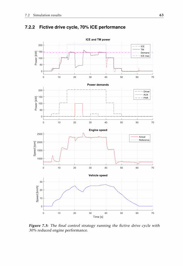
• Chapter 7 - ResultsPresents the final control strategy together with simulation results with thisstrategy implemented.

• Chapter 8 - DiscussionThe results and insights from the work are discussed.

• Chapter 9 - Conclusions & Future WorkThe conclusions drawn from the work are summarized and suggestions forfuture work are given.

2The Diesel-Electric Powertrain

The diesel-electric powertrains from BAE System Hägglunds AB are typicallyused in low speed, high torque applications. Two examples of these applicationsare reachstackers and aircraft tow trucks, as shown in Figure 2.1. In a conven-tional diesel powertrain for these applications, mechanical power from the ICEis transmitted through shafts and other mechanical components to the driveshaft,see Figure 2.2. In a diesel-electric powertrain on the other hand, the mechanicalpower from the ICE is first converted into electrical power in a generator andthen transmitted through cables to an electric traction motor. This motor is, inturn, mechanically connected to the driveshaft, see Figure 2.3.

(a) (b)

Figure 2.1: Typical applications of BAE Systems Hägglunds diesel-electricpowertrains: (a) reachstackers and (b) aircraft tow trucks (NOTE: these pic-tures are included after approval from their respective originators).

5

6 2 The Diesel-Electric Powertrain

W

ICE FATTC

W

Figure 2.2: Simplified schematic of a conventional diesel powertrain. Thepower is transmitted from the internal combustion engine (ICE) to thewheels (W) through shafts and other mechanical components (TC = torqueconverter, AT = automatic transmission, F = final drive).

W

ICE F

W

GEN TM

Figure 2.3: Simplified schematic of a diesel-electric powertrain. Mechanicalpower from the internal combustion engine is converted into electric powerin a generator (GEN). It is then transmitted through cables to an electric trac-tion motor (TM) which is mechanically connected to the wheels (W), usuallythrough a final drive (F).

In a diesel-electric powertrain configuration, the wheels are mechanically de-coupled from the ICE, which comes with several advantages.

• Another degree of freedom is introduced when the ICE speed can be freelychosen regardless of the vehicle speed.

• Bigger freedom regarding the physical placement of the ICE, since routingof electrical cables usually is a less complex concern compared to connect-ing the components mechanically.

• The electric traction motor allows for maximum torque output from stand-still.

2.1 System description 7

These advantages typically come at a cost of reduced driveline efficiency sincethe required energy conversions introduce losses. Another disadvantage with adiesel-electric powertrain is of economical nature; the components of the power-train are usually more expensive compared to the conventional counterparts.

2.1 System description

In Figure 2.3, a greatly simplified schematic of a general diesel-electric power-train was presented. In this section, a more detailed description of the studiedpowertrain is given.

ICE GEN TM

GCU

~ ~

PCM

AUX

ECU

~=

TCU

~=

Driver reference

PAR

⎓

Figure 2.4: A more detailed schematic of the studied powertrain, includingpower electronics, controllers, control signals and also auxiliary and par-asitic loads connected to the DC bus. The components downstream fromthe traction motor (TM) are omitted. Thick lines represent electric powertransmission and narrow lines control and/or measurement signals. Darkgrey blocks represent high-power components and light grey blocks controlunits. Dashed, light gray boxes highlight coherent subsystems.

Figure 2.4 shows a schematic of the studied powertrain. Below, brief descrip-tions of the components are given.

• Internal combustion engine (ICE) with engine control unit (ECU)A diesel engine produces crankshaft torque and is controlled with its ECU.


These two components are delivered together as a coherent subsystem. Theengine considered in this thesis is a turbocharged Cummins™ 6-cylinder6.7-litre engine with fixed-geometry turbine and wastegate for boost con-trol. The maximum ICE power is 205 kW.

• Generator (GEN), inverter and generator control unit (GCU)A generator converts the mechanical power from the ICE to 3-phase AC elec-trical power, which is then converted to DC using an inverter. The two com-ponents are controlled with a generator control unit. These components areworking together as a coherent subsystem.

• DC busThe DC power transmission between the inverters is referred to as the DCbus. The nominal voltage in this bus is typically around 750 V.

• Traction motor (TM), inverter and traction control unit (TCU)The DC power in the DC bus is inverted to AC and then fed to the tractionmotor. The two components are controlled via a traction control unit, andtogether they form a subsystem.

• Auxiliary load (AUX)The main external load, referred to as the AUX load, is typically a high-power hydraulic demand in the reachstacker case. This load consumespower from the DC bus and its magnitude is known to the PCM. The maxi-mum AUX load is 100 kW.

• Parasitic load (PAR)Similar to the AUX load, a parasitic load with a maximum magnitude of 20kW may consume power from the DC bus. The difference from the AUXload is that the magnitude of the PAR load is not known to the PCM.

• Powertrain control module (PCM)The powertrain control module is the superior control node for the wholepowertrain. It uses driver input and measured signals to set out appropriatereference signals to the ECU, GCU and TCU. The control strategy logic isimplemented in this unit.

2.2 Control

As shown in Figure 2.4, the ICE and the electric machines all have individualcontrol units. These control units can operate in different control modes. De-scriptions of these modes are presented in this section.

2.2.1 ECU

The ECU follows the SAE J1939 standard [1]. In this thesis, two control modesare of interest.

2.2 Control 9

• Torque control : given a torque reference, the ECU calculates the corre-sponding amount of fuel needed. As stated in the standard, the referencetorque is interpreted as an indicated torque (as opposed to a braking torque),implying that no friction and pump loss compensation is done.

• Speed control : given a speed reference, the ECU controls the speed of theengine.

2.2.2 GCU & TCU

The GCU and TCU have three different operating modes.

• Torque control : given a torque reference, the control unit controls the shafttorque of the electric machine

• Speed control : given a speed reference, the control unit controls the shaftspeed of the electric machine

• Voltage control : given a reference voltage, the control unit controls the volt-age in the DC bus

Block diagrams of these control modes are shown in Figure 2.5.

EM~

=

FOC

TEM,ref

EM~

=

FOC

ωEM,ref

iAC

ω control

ωEM

EM~

=

FOC

UDC,ref

U control

UDC

iACiAC

Torque control mode Speed control mode Voltage control mode

CU

CU CU

TEM,ref

+- +-

TEM,ref

Figure 2.5: Control modes of the inverters. The electric machine (EM) torqueis controlled by field-oriented control (FOC), which is not explained fur-ther in this thesis. More information regarding this control principle canbe found in [11] and [19]. The dashed grey rectangles represent the controlunits (CU).

Controller parametrization

The control parameters in the GCU and TCU controllers can be individually setat runtime through CAN messages.


LimitRegenPower & LimitMotoringPower

It is possible to set limits on how much regenerative and motoring power theGCU and TCU should allow the electric machines to produce through CAN mes-sages. These messages are called LimitRegenPower and LimitMotoringPower, re-spectively.

2.2.3 Control limitations due to subsystem boundaries

In an ideal, academic context any control law can be applied anywhere in thesystem. However, in the applied case studied in this thesis, this is not possibledue to how subsystems are delivered as coherent components from external sup-pliers. With limited communication interfaces between units and predeterminedcontrol logic in the delivered controllers, the design freedom is greatly reduced.These limitations could theoretically be circumvented by developing the subsys-tem control units (ECU, GCU, TCU) completely from scratch, but this is not prac-tically feasible due to the immense cost this would imply. For this reason, the useof standard components is strived for in the highest possible extent.

2.3 Communication

The PCM communicates with the other control units via a controller area network(CAN) bus. The communication is not instantaneous but occurs with a nominalmaximum cycle time between messages. Prioritization mechanisms then ensurethat the nominal maximum cycle time is not exceed.

The nominal cycle time is set to 10 ms for all messages in this thesis.

2.4 Established control strategy (CS1)

With the established control strategy, referred to as control strategy 1 (CS1), themain idea is that the driver is in control of the traction torque, while the generatortakes care of voltage control and the engine controls the engine speed. Both thevoltage control and speed control are realized on subcomponent level in the GCUand ECU, respectively. A block diagram showing this strategy is presented inFigure 2.6.

2.4.1 Torque reduction

The nominal maximum power of the ICE is known to the PCM. Hence, the trac-tion power can be saturated to not exceed this value. However, if the ICE hasreduced performance due to for example high altitude driving conditions or en-gine malfunction, the actual maximum power is lower. This actual value is un-known to the PCM. If the TM consumes more power than the ICE can produce,the engine will decelerate and ultimately stall.

2.4 Established control strategy (CS1) 11

ECU

PCM

GCU

ICE GEN TM

Uref

U control

+ -

ω control

ωref Driver interpretation & speed selection

αap

MTM,ref

+ -

Torque reduction

MTM,des

+-

ωerr

Figure 2.6: Simplified block diagram of the established control strategy(CS1) where power electronics and FOC blocks have been omitted for sim-plicity.

To circumvent this problem, a traction torque reduction is used. The TMtorque is reduced proportionally to the engine speed error ωerr with a deadbandωdb. This technique can be mathematically described with

MTM,ref = MTM,des − kp,redωred (2.1)

ωred =

ωerr − ωdb, if ωerr − ωdb > 00, otherwise

(2.2)

where MTM,ref is the actual torque reference to the TM, MTM,des the torque de-sired by the driver, ωerr = ωref −ω the engine speed error and ωdb the deadband.In this way, the TM will decrease its torque until a stationary operating point isreached, thereby preventing the engine to stall.

2.4.2 Pull analogy

When the driver demands torque from the TM, the voltage in the DC bus willdrop as a consequence of the increased power consumption. To counteract this,the GEN, being the voltage controlling unit, will start to load the engine shaftand feed power into the bus. This will decelerate the shaft and thus increasethe speed error, which will cause the ECU to increase the produced ICE torque


in order to maintain the speed. In summary, the driver initiates power outputfrom the consuming side of the powertrain and gets the components upstreamto produce the corresponding power. Hence, this strategy can be seen as a pullstrategy. In Figure 2.7, this principle is visualized.

ICE GEN TM

3 2 1

Figure 2.7: Schematic demonstrating the pull principle. The driver initiatespower consumption in the TM (1) causing the voltage to drop. The GENresponds to the decreasing voltage by loading the engine shaft and feedingpower into the DC bus (2) causing the shaft to decelerate. Finally, the ICEreacts to the declining shaft speed by producing the required power (3).

2.4.3 Maximum power utilization problem

The main problem with CS1 is utilizing the full power available from the engine.As described in Section 2.4.1, the maximum engine power might be time-varyingdue to for example engine malfunctioning or high-altitude driving conditionsand is therefore unknown to the PCM. When the power consumed by the TM ex-ceeds the maximum power currently available from the ICE, the engine will de-celerate, the speed error increase and the torque reduction eventually kick in. Ul-timately, the powertrain will reach a stationary operating point when the torquereduction is of sufficient size. When this occurs, however, the engine speed willsettle with a constant error since the reduction is purely proportional (comparewith a proportional controller). A lower engine speed implies that an even lowermaximum power will be available from the ICE due the shape of its maximumpower curve (typically increasing maximum power with increasing engine speed).Hence, even if the driver requests full power only part of it will be produced.

This problem is demonstrated in Figure 2.8. In (a) the engine has the full nom-inal power available (205 kW) and it is seen that the traction power reaches upto and settles at the desired level. In (b) however, engine performance is reducedby 30%, leading to a maximum power of 143.5 kW. In this case, the tractionpower settles at a lower-than-available level (approximately 117 kW) and the en-gine speed establishes a significant constant error. So, even though the driverrequests maximum available power only approximately 82% of it is delivered.

2.5 Proposed control strategy (CS2) 13

0 5 10 15

0

50

100

150

200

Pow

er [k

W]

CS1 @ 100% ICE performanceTraction power

Traction power

Demanded power

Max engine power

0 5 10 15

Time [s]

1000

1500

2000

2500

Spe

ed [r

pm]

Engine speed

Actual speedReference speed

(a)

0 5 10 15

0

50

100

150

200

Pow

er [k

W]

CS1 @ 70% ICE performanceTraction power

Traction power

Demanded power

Max engine power

0 5 10 15

Time [s]

1000

1500

2000

2500

Spe

ed [r

pm]

Engine speed

Actual speedReference speed

(b)

Figure 2.8: The main problem with CS1 demonstrated using a step in de-manded power from 0% to 100%. In (a) the engine has the full nominalpower available (205 kW), while in (b) the maximum power is reduced by30% to 143.5 kW.

2.5 Proposed control strategy (CS2)

In order to circumvent the problem with CS1, a new control approach is pro-posed. The principal idea is to invert the control structure; instead of having thedriver control the traction motor (i.e. the power consuming part of the power-train), the driver controls the engine (i.e. the power producing part). Meanwhile,the GEN takes care of engine speed control and the TM realizes voltage control.A block diagram of the proposed control strategy is presented in Figure 2.9.

2.5.1 Push analogy

When the driver initiates torque generation from the ICE, the shaft will start toaccelerate. The GEN, being the speed controlling component, will counteract thisacceleration by loading the shaft with a braking torque in order to keep the speedat the desired level. This will in turn feed power into the DC bus and cause thevoltage to increase. The TM will therefore start to consume power by generatingtorque in order to keep the voltage at the reference level, and traction is achievedconsequently. Hence, CS2 can be seen working according to a push principle.This concept is visualized in Figure 2.10.

An interesting remark is that the proposed control strategy is analogous to the


TCU

PCM

GCU

ICE GEN TM

Uref

ω control

+-

U control

ωref

Driver interpretation & speed selection

αap

+-

MICE,ref

Figure 2.9: Block diagram of the proposed control strategy (CS2).

ICE GEN TM

1 2 3

Figure 2.10: Schematic demonstrating the push principle. The driver con-trols the ICE to produce power (1) causing the shaft to accelerate. The GENresponds to this acceleration by loading the shaft and feeding power into theDC bus (2), which causes the voltage to increase. Finally, the TM counteractsthe increasing voltage by consuming power from the bus and thus generatingtraction (3).

way a conventional diesel powertrain is controlled; the driver has control over thepower producer in the powertrain (the ICE) instead of the power consumer (thewheels). By initiating torque generation from the engine, traction is obtainedconsequently.

3Approach

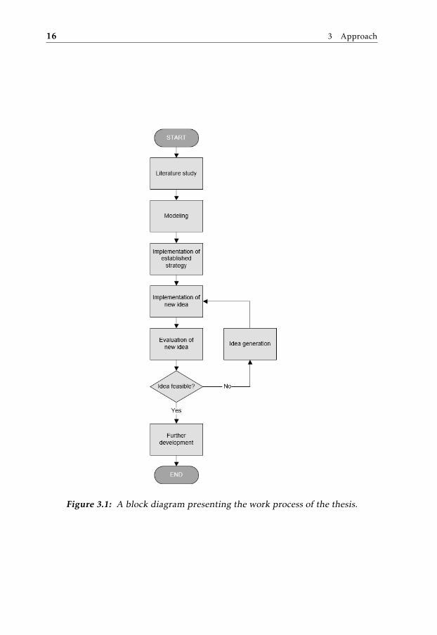
This chapter presents the approach and working process of the thesis. The workis divided into a number of different phases, which are explained below. A visualrepresentation of the process is shown in Fig 3.1.

1. Literature studyA study of related research is conducted in order to find out what work hasbeen done in the field, state-of-the-art technologies, and so forth.

2. ModelingIn order to have a plant model to develop and evaluate the control strate-gies on, such a model is compiled. The model is implemented in MAT-LAB™/Simulink™.

One major component that have been simplified in previous models is theICE. Thus, a new model for this component is implemented in order tocatch dynamic phenomena such as the turbocharger dynamics. In [15] avalidated model for a similar diesel-electric powertrain is developed andpresented. In [4] an optimal-control oriented MATLAB™ implementationof this model is provided under the name LiU-D-El which is implementedduring the modeling phase.

3. Implementation of established strategyA control strategy working according to the established approach is imple-mented in order to reproduce the problem of interest.

4. Control strategy developmentStarting with the proposed control approach, a development loop is iter-ated. After implementing the initial idea, the performance and characteris-tics of the approach are evaluated and a new, refined idea is generated. Theprocedure is then repeated.

15

16 3 Approach

Figure 3.1: A block diagram presenting the work process of the thesis.

3.1 Drive cycles 17

5. Further developmentWhen a promising control approach is found, the development loop is ex-ited and the final idea further refined.

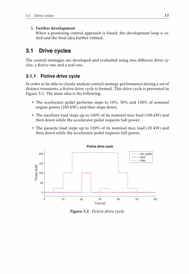
3.1 Drive cycles

The control strategies are developed and evaluated using two different drive cy-cles: a fictive one and a real one.

3.1.1 Fictive drive cycle

In order to be able to clearly analyze control strategy performance during a set ofdistinct transients, a fictive drive cycle is formed. This drive cycle is presented inFigure 3.2. The main idea is the following:

• The accelerator pedal performs steps to 10%, 50% and 100% of nominalengine power (205 kW), and then steps down.

• The auxiliary load steps up to 100% of its nominal max load (100 kW) andthen down while the accelerator pedal requests full power.

• The parasite load steps up to 100% of its nominal max load (20 kW) andthen down while the accelerator pedal requests full power.

0 10 20 30 40 50 60

Time [s]

0

50

100

150

200

Pow

er

[kW

]

Fictive drive cycle

Acc. pedal

AUX

PAR

Figure 3.2: Fictive drive cycle.

18 3 Approach

3.1.2 Real drive cycle

The second drive cycle is from a real driving scenario. The accelerator pedal andAUX signals have been recorded for a longer period of time during real driving,and a 273 second excerpt from these recordings are used as a more realistic driv-ing mission. This drive cycle is shown in Figure 3.3.

0 50 100 150 200 250

0

0.2

0.4

0.6

0.8

1

Acc.

pe

da

l p

ositio

n [

-]

0 50 100 150 200 250

Time [s]

0

0.2

0.4

0.6

0.8

1

AU

X p

ed

al p

ositio

n [

-]

Figure 3.3: Real drive cycle.

4Related Research

4.1 Control

A diesel-electric powertrain is not a hybrid powertrain since it uses only onesource of energy. Though, its layout is similar to the one of a series hybrid electricpowertrain. The main difference between the two is that the latter, in additionto chemical fuel storage, also has an electric energy storage which can supplypower to the electric bus. Thus, control of a diesel-electric powertrain shouldbe similar to control of a series hybrid electric powertrain when the electric en-ergy storage is empty and/or non-utilizable. This mode of operation is describedas “Engine/Generator-Alone Traction Mode” in [5] and [10]. However, this op-erating mode is seemingly not the preferred operating mode in such a power-train, which is obvious in [10] where the propulsion system of a series hybridelectric vehicle (SHEV) is described as “an electric motor with batteries that canbe charged through a generator driven by an ICE”. Hence, the primary functionof the engine-generator set is not powering the traction motors directly.

Seemingly, there is a relatively scarce amount of research that has been con-ducted regarding control of purely diesel-electric powertrains when compared tothe field of SHEVs. Thus, it is of interest to investigate how SHEVs are controlledin the operating mode described above. However, the majority of the publica-tions found regarding control of SHEVs cover control strategies for energy man-agement in the vehicle, for example how to control the state-of-charge (SOC) inthe battery pack, which is a completely different problem (Barsali et al. presentsthis control problem in a good way in [2]). This further speaks for the main pur-pose of the engine-generator set (GENSET) being charging the batteries as statedin [10], rather than directly providing power to the traction motors.

Two applications for diesel-electric powertrains are railroad locomotives andmarine ships [12], [3]. In the marine case, diesel-electric propulsion started to

19

20 4 Related Research

gain popularity in the 1980s when advances in switching power electronic tech-nology made new ways of variable speed control of electric motors possible [8].Since then, a considerable amount of research work has been carried out aboutelectric propulsion in marine vessels. In [7], Geertsma et al. presents a thor-ough summary of different marine propulsion architectures, including the fea-tures and layout of the electrical propulsion architecture. From this summary, itis obvious that a typical diesel-electric powertrain in a marine application resem-bles the powertrain studied in this thesis, but also has several differences. Oneimportant difference is the power distribution system: in marine applications,the electrical power is usually distributed on a fixed-frequency AC grid while thestudied powertrain has a DC bus. However, Hansen and Wendt [8] state that DCtransmission on marine vessels is a promising new solution.

The summary of marine electrical propulsion in Geertsma et al. [7] shows thatthe common way to control a marine diesel-electric powertrain is to control thespeed of the engines to provide the desired grid frequency, control the generatorto maintain a certain voltage and then control the electric motors to keep upa desired propeller speed. Thus, this resembles a pull strategy similar to theestablished strategy for the studied powertrain. There are two main differencesthough.

• In the marine case, the demand signal from the driver is a speed reference,while it is a torque reference in the studied case. However, research hasshown that torque/power control of the shaft might be advantageous [18].If torque control was used in such a powertrain, its control strategy wouldbe principally very similar to the established strategy in the studied power-train.

• The engine speed in the marine application has to be fixed in order to pro-duce AC power with the appropriate frequency for the AC grid. In the stud-ied application, where a DC grid is used, the engine speed can be freelychosen since the provided frequency is not of importance.

A particular interest during the literature study has been whether the pro-posed push principle has been previously investigated or not. However, power-train control according to this approach has not been encountered during thestudy.

4.2 Modeling

Since the secondary purpose of the thesis is to compile a powertrain model witha more sophisticated ICE model incorporating turbocharger dynamics, the im-portance of such an incorporation has been investigated. In [13], Nezhadali et al.conclude that omitting the turbocharger dynamics in models for transient timeand fuel consumption calculations can incur underestimates of both time andconsumption of over 60% in transients.

There has been extensive research done within the field of modeling of tur-bocharged internal combustion engines. Eriksson and Nielsen thoroughly presents

4.2 Modeling 21

methodology for both modeling and control of engines and drivelines in [6], us-ing the work from over 300 relevant publications and textbooks.

In [20], Eriksson and Wahlström presents a full mean-value model of a tur-bocharged diesel engine with variable-geometry turbine and exhaust gas recir-culation, and also provide a Simulink™ implementation of the model. Eventhough the studied powertrain has an engine with fixed-geometry turbochargerand wastegate for boost control, big parts of the work from Eriksson and Wahlströmmight be relevant in this case, allowing for model re-usage and a potential de-crease in the amount of model development effort needed.

Regarding modeling of diesel-electric powertrains specifically, Sivertsson andEriksson present a validated model of a diesel-electric powertrain in [15]. Themodel is developed with focus on optimal control and covers the engine-generatorset only, but might surely be useful throughout this thesis. For example, thismodel describes the same turbocharger configuration as in the studied case (fixed-geometry turbine with wastegate), which could be a better basis than the modelin [20] for this thesis.

The same Sivertsson and Eriksson also investigate optimal transient controltrajectories in diesel-electric systems in [16] and [17]. The conclusions from thesepublications might be used in controller design to tackle the problem of how tooptimally move the operating point of the diesel engine between different powerlevels.

Regarding modeling of diesel-electric powertrains in general, Hansen et al.presents a mathematical model of such a powertrain in [9]. The modeled pow-ertrain has an AC distribution grid (as most marine vessels with diesel-electricpropulsion do) and thus, it is principally different from the studied powertrain.However, even though the model itself might be irrelevant, modeling and controlconcepts used in the work is of interest for this thesis.

5Modeling

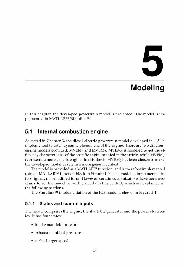
In this chapter, the developed powertrain model is presented. The model is im-plemented in MATLAB™/Simulink™.

5.1 Internal combustion engine

As stated in Chapter 3, the diesel-electric powertrain model developed in [15] isimplemented to catch dynamic phenomena of the engine. There are two differentengine models provided, MVEM0 and MVEM2. MVEM0 is modeled to get the ef-ficiency characteristics of the specific engine studied in the article, while MVEM2represents a more generic engine. In this thesis, MVEM2 has been chosen to makethe developed model usable in a more general context.

The model is provided as a MATLAB™ function, and is therefore implementedusing a MATLAB™ function block in Simulink™. The model is implemented inits original, non-modified form. However, certain customizations have been nec-essary to get the model to work properly in this context, which are explained inthe following sections.

The Simulink™ implementation of the ICE model is shown in Figure 5.1.

5.1.1 States and control inputs

The model comprises the engine, the shaft, the generator and the power electron-ics. It has four states:

• intake manifold pressure

• exhaust manifold pressure

• turbocharger speed

23

24 5 Modeling

• engine speed

and three control signals:

• injected fuel mass

• wastegate position

• generator power

In this thesis, both the shaft and the generator are modeled individually. Thus,the engine speed state is not used and the generator power control signal is set tozero.

5.1.2 Internal signals and outputs

From the original model, there are five output signals: derivatives of the fourstates and a struct c with additional quantities. Since the main aspect of interestin this context is the torque generation, another output signal Mice with the en-gine torque is added. Also, an output signal mci with the cylinder-in mass flow isadded since it is needed both for lambda calculation and in the ECU model.

Figure 5.1: Simulink™ implementation of the LiU-D-El model.

5.2 ECU 25

5.1.3 State and control signal normalization

The provided model works with normalized values for both the states and the con-trol signals. Thus, a normalizing/denormalizing layer has to be wrapped aroundthe MATLAB™ function, making use of norm values which are all provided to-gether with the model.

5.1.4 Maximum torque limit

The engine net torque Mice is saturated using the maximum torque curve, ensur-ing the engine model does not generate a higher torque than physically possible.

5.2 ECU

As described in Section 2.2.1 the ECU control modes of interest in this thesis aretorque control and speed control. These are implemented together with a modesignal in order to enable mode switching as desired.

5.2.1 Fuel feed-forward

From the torque request coming either directly from the PCM or from the ECUspeed controller, the required fuel mass to be injected is calculated. An inversionof the engine torque model for the indicated gross torqueMig as described in [15]is used, according to

Mig =uf ncylqHV ηig

4π⇒ uf =

4πMig

ncylqHV ηig(5.1)

where ηig is calculated as

ηig = ηig,t

1 − 1

rγcyl−1c

(5.2)

and ηig,t as

ηig,t = ηig,ch + cuf ,1

(ufωice

)2

+ cuf ,2ufωice

(5.3)

The parameter data provided with the model are used for the parameters inthe above expressions.

5.2.2 Smoke limiter

In diesel engines, the air-fuel equivalence ratio λ should not be allowed to fall be-low a certain level to prevent smoke (particulate matter) generation, as describedin [6]. Thus, a smoke limiter is implemented to limit the amount of fuel injecteddepending on how much air is available for the combustion. The desired fuel

26 5 Modeling

mass uf ,des is limited with respect to the maximum allowed fuel mass uf ,max ac-cording to

uf = min(uf ,des, uf ,max(mci , ωice)) (5.4)

In this equation, uf ,max(mci , ωice) is calculated as

uf ,max(mci , ωice) =4πmci

ωice(A/F)sλminncyl(5.5)

where mci is the cylinder in mass flow, ωice the engine speed,(A/F)s the stoichio-metric air-fuel ratio, λmin the lower limit on λ and ncyl the number of cylinders.

5.2.3 Low idle governor

According to the SAE J1939 standard [1], the ECU will not let the engine stallwhen controlled in torque control mode. When zero torque is requested, the en-gine will decelerate until the shaft speed drops below a certain low idle speed.At this point, a low idle governor (LIG) kicks in to prevent stalling. Accordingto the standard, this governor can be implemented either using a maximum se-lection technique or a summation technique (described in figures SPN512_A andSPN512_B in the standard, respectively). In this thesis, the LIG is implementedusing the maximum selection principle as a proportional controller, contributingwith a torque request to the engine whenever the speed drops below the reference,according to

Mref = max(Mref ,des, kp,LIGωerr ) (5.6)

where kp,LIG is the proportional gain of the LIG and ωerr is the speed errorrelative to the low idle speed.

5.2.4 Wastegate control

Control of the wastegate in turbocharged ICEs is a non-trivial matter. There areseveral possible principles that can be used, all having their advantages and dis-advantages. In this thesis, where wastegate control is not the topic of interest,just a simple technique is enough in order to get sufficiently realistic engine be-havior. Thus, a simplified control approach is used, where a PI controller actuatesthe wastegate to keep the air-fuel equivalence ratio λ at a specified setpoint. Inthis way, the wastegate will be open at stationary operating points (minimizingthe back pressure and hence the fuel consumption) and closed during transientswhen more air is needed. This is considered to be a close-to-realistic behavior.

5.3 Genset shaft 27

5.3 Genset shaft

The rotational speed of the genset shaft is modeled using Newton’s second lawfor rotation, that is

Mice −Mgen = Jgensetω (5.7)

where Mice is the engine torque, Mgen the generator torque, Jgenset the mo-ment of inertia of the GENSET and ω the rotational speed.

5.4 Generator, traction motor & inverters

The generator and the traction motor with their respective inverters are bothmodeled in the same way. They are simplified as first order systems with timeconstants of 10 ms, with transfer functions according to

Mem =1

τems + 1Mref (5.8)

where Mem is the actual torque produced by the EM, τem is the time constantand Mref is the requested torque. This simplification is motivated with the factthat the dynamics of the EMs are significantly faster than the dynamics of theICE, making the later the limiting component.

5.5 GCU/TCU

The generator and traction motor control units are very similar in functionalityand are therefore modeled in the same manner. As described in Section 2.2.2,these control units can operate in either torque, speed or voltage control mode.These modes are all implemented together with a mode signal, making it possibleto select operating mode from the PCM.

The output from the GCU/TCU is a reference torque to their respective elec-tric machine models. Thus, the torque control mode is implemented simplyas a direct forwarding from input reference torque to output reference torque.The speed and voltage controllers are then implemented as superior controllersoutputting reference torque as control signals. Additionally, the LimitRegen-Power and LimitMotoringPower signals described in Section 2.2.2 are also imple-mented.

The Simulink™ model of the GCU is presented in Figure 5.2 for clarity.

28 5 Modeling

Figure 5.2: Simulink™ model of the GCU. The TCU model is identical exceptsign conventions.

5.6 DC bus

The DC bus voltage is modeled using the relationship between current and volt-age in a capacitive circuit

i(t) = Ctotdv(t)

dt⇒ v(t) =

∫1Ctot

i(t) dt (5.9)

where i(t) is the current, v(t) the voltage and Ctot the total capacitance of theDC bus. Combining this expression with the power relation

P (t) = v(t) i(t) ⇒ i(t) =P (t)v(t)

(5.10)

yields

v(t) =∫

1Ctot

P (t)v(t)

dt (5.11)

where P (t) is the sum of all incoming (+) and outgoing (-) powers with signs.This gives the final expression

v(t) =1Ctot

∫Pgen(t) − Ptm(t) − Paux(t) − Ppar (t)

v(t)dt (5.12)

5.7 Drive shaft & vehicle 29

5.7 Drive shaft & vehicle

The drive shaft speed is modeled in a similar way as the genset shaft, using New-ton’s second law for rotation. There are however two main differences.

5.7.1 Simplified loss assumption

The braking torque on the drive shaft comes from the driving resistance of thevehicle. A simplified loss assumption is made, yielding that the driving resis-tance (comprising air drag, rolling resistance, and so forth) is proportional to thevehicle speed and thus also to the drive shaft speed, that is

Mbr = γωd (5.13)

where Mbr is the braking torque on the shaft, γ the loss factor and ωd thedrive shaft speed.

5.7.2 Reflected inertia

The mass of the vehicle reflects as moment of inertia on the drive shaft. Theexperienced moment of inertia that the TM effectively drives is

Jexp =Jvehi2d

+ Jd (5.14)

where

Jveh = mvehr2w (5.15)

and id is the final drive gear ratio, Jd the drive shaft moment of inertia, mveh thevehicle mass and rw the wheel radius.

5.8 Bus communication

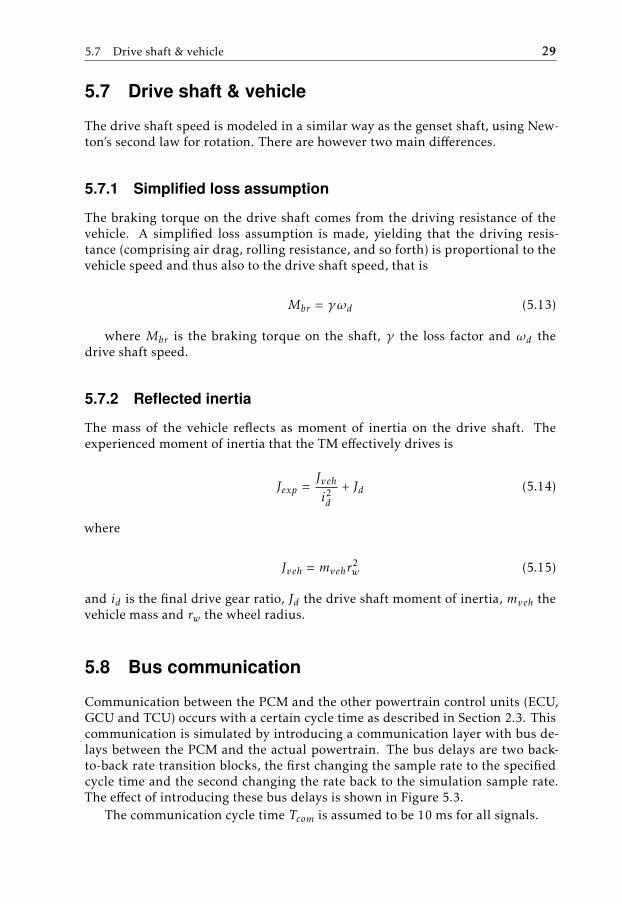
Communication between the PCM and the other powertrain control units (ECU,GCU and TCU) occurs with a certain cycle time as described in Section 2.3. Thiscommunication is simulated by introducing a communication layer with bus de-lays between the PCM and the actual powertrain. The bus delays are two back-to-back rate transition blocks, the first changing the sample rate to the specifiedcycle time and the second changing the rate back to the simulation sample rate.The effect of introducing these bus delays is shown in Figure 5.3.

The communication cycle time Tcom is assumed to be 10 ms for all signals.

30 5 Modeling

0 0.2 0.4 0.6 0.8 1

Time [s]

-1

-0.5

0

0.5

1

[-]

Effect of bus delay

Original signalWith bus delay

Figure 5.3: Effect of introducing a bus delay, demonstrated on a sine wavesignal.

5.9 Model validation

Since no data from the real powertrain is available, validating the model againstreal measurements is not possible. Instead the model is validated by assessingthe model behavior and confirming that it complies with the expected behavior.This validation is done both for the individual subsystems and for the completepowertrain with CS1 implemented.

5.9.1 ECU & ICE

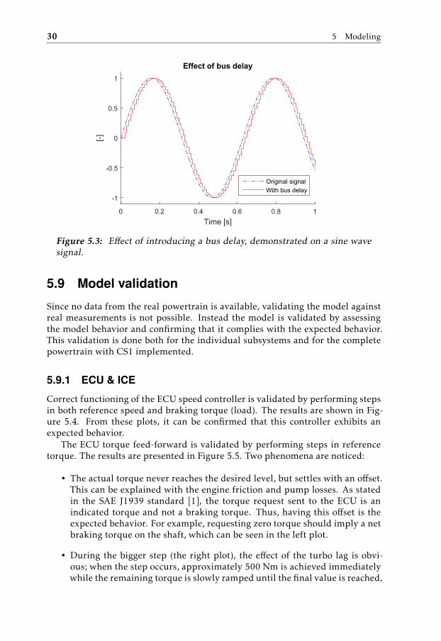
Correct functioning of the ECU speed controller is validated by performing stepsin both reference speed and braking torque (load). The results are shown in Fig-ure 5.4. From these plots, it can be confirmed that this controller exhibits anexpected behavior.

The ECU torque feed-forward is validated by performing steps in referencetorque. The results are presented in Figure 5.5. Two phenomena are noticed:

• The actual torque never reaches the desired level, but settles with an offset.This can be explained with the engine friction and pump losses. As statedin the SAE J1939 standard [1], the torque request sent to the ECU is anindicated torque and not a braking torque. Thus, having this offset is theexpected behavior. For example, requesting zero torque should imply a netbraking torque on the shaft, which can be seen in the left plot.

• During the bigger step (the right plot), the effect of the turbo lag is obvi-ous; when the step occurs, approximately 500 Nm is achieved immediatelywhile the remaining torque is slowly ramped until the final value is reached,

5.9 Model validation 31

0 5 10 15

Time [s]

1000

1500

2000

2500

Spe

ed [r

pm]

Speed step (800 -> 2400 rpm)at constant load (100 Nm)

ActualReference

0 5 10 15

Time [s]

1000

1200

1400

1600

1800

2000

Spe

ed [r

pm]

Load step (200 -> 600 Nm)at constant speed (1600 rpm)

ActualReference

Figure 5.4: Validation of proper functioning of the ECU speed controller.

0 2 4 6 8 10

Time [s]

-100

-50

0

50

100

150

200

250

Tor

que

[Nm

]

Torque step (0 -> 200 Nm)at constant speed (1400 rpm)

ActualReference

0 2 4 6 8 10

Time [s]

200

300

400

500

600

700

800

Tor

que

[Nm

]Torque step (300 -> 800 Nm)at constant speed (1400 rpm)

ActualReference

Figure 5.5: Torque step responses for the ICE.

taking a couple of seconds. This is due to an initial lack of air for the com-bustion, which is counteracted as the turbocharger speeds up and causes ahigher intake manifold pressure.

5.9.2 GCU/TCU

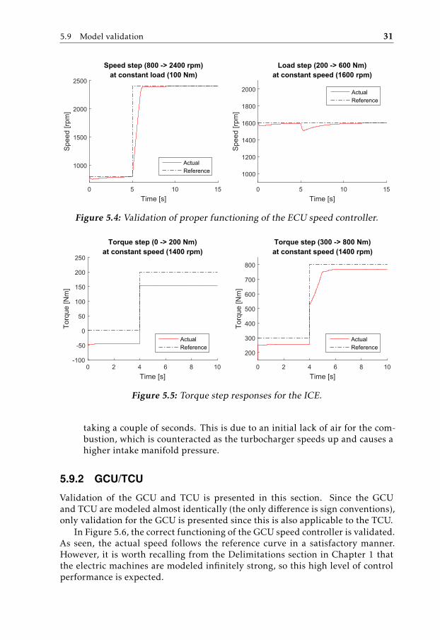
Validation of the GCU and TCU is presented in this section. Since the GCUand TCU are modeled almost identically (the only difference is sign conventions),only validation for the GCU is presented since this is also applicable to the TCU.

In Figure 5.6, the correct functioning of the GCU speed controller is validated.As seen, the actual speed follows the reference curve in a satisfactory manner.However, it is worth recalling from the Delimitations section in Chapter 1 thatthe electric machines are modeled infinitely strong, so this high level of controlperformance is expected.

32 5 Modeling

0 5 10 15

Time [s]

800

1000

1200

1400

1600

1800

2000

2200

Spe

ed [r

pm]

Speed step (1000 -> 2000 rpm)at constant load (200 Nm)

ActualReference

0 5 10 15

Time [s]

800

1000

1200

1400

1600

1800

2000

2200

Spe

ed [r

pm]

Load step (100 -> 400 Nm)at constant speed (1500 rpm)

ActualReference

Figure 5.6: Validation of correct functioning of the GCU speed controller. Inthe left plot a step in reference speed is performed, and in the right plot astep in torque on the incoming shaft is performed.

0 2 4 6 8 10

Time [s]

680

700

720

740

760

780

800

820

Vol

tage

[V]

Step in load (20 -> 80 kW)at constant voltage (750 V)

ActualReference

0 2 4 6 8 10

Time [s]

680

700

720

740

760

780

800

820

Vol

tage

[V]

Step in load (140 -> 200 kW)at constant voltage (750 V)

ActualReference

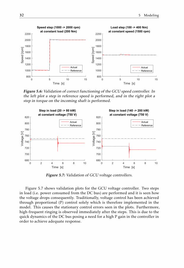
Figure 5.7: Validation of GCU voltage controllers.

Figure 5.7 shows validation plots for the GCU voltage controller. Two stepsin load (i.e. power consumed from the DC bus) are performed and it is seen howthe voltage drops consequently. Traditionally, voltage control has been achievedthrough proportional (P) control solely which is therefore implemented in themodel. This causes the stationary control errors seen in the plots. Furthermore,high-frequent ringing is observed immediately after the steps. This is due to thequick dynamics of the DC bus posing a need for a high P gain in the controller inorder to achieve adequate response.

5.9 Model validation 33

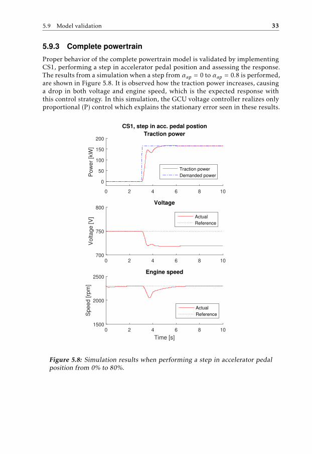
5.9.3 Complete powertrain

Proper behavior of the complete powertrain model is validated by implementingCS1, performing a step in accelerator pedal position and assessing the response.The results from a simulation when a step from αap = 0 to αap = 0.8 is performed,are shown in Figure 5.8. It is observed how the traction power increases, causinga drop in both voltage and engine speed, which is the expected response withthis control strategy. In this simulation, the GCU voltage controller realizes onlyproportional (P) control which explains the stationary error seen in these results.

0 2 4 6 8 10

0

50

100

150

200

Po

we

r [k

W]

CS1, step in acc. pedal postion

Traction power

Traction power

Demanded power

0 2 4 6 8 10700

750

800

Vo

lta

ge

[V

]

Voltage

Actual

Reference

0 2 4 6 8 10

Time [s]

1500

2000

2500

Sp

ee

d [

rpm

]

Engine speed

Actual

Reference

Figure 5.8: Simulation results when performing a step in accelerator pedalposition from 0% to 80%.

6Control Strategy Development

6.1 Proposed strategy (CS2)

The proposed control strategy as described in Chapter 2 is implemented in Simulink™.The approach exhibits two main problems.

6.1.1 Voltage control at standstill

In CS2, the TM is the voltage controlling actuator. Thus, it needs to be capableof both decreasing and increasing the voltage as necessary. A voltage decrease isachieved by generating accelerating torque on the drive shaft and hence consum-ing power from the DC bus. A voltage increase is achieved in the opposite way;the TM loads the drive shaft with a decelerating torque and regenerates power tothe DC bus.

When the vehicle stands still (i.e. vveh = 0) there is no kinetic energy availablefor the TM to use for increasing the DC voltage. Since the TM is the only voltagecontrolling unit, the voltage will drop if the ICE is not producing any power. Thisproblem is confirmed in Figure 6.1.

6.1.2 Voltage control at no traction demand

As described in the previous section, the problem at standstill is to increase thevoltage. When the driver requests no traction (i.e. the accelerator pedal positionis zero, αap = 0), another similar problem occurs. Requesting zero traction mustof course imply zero traction torque and thus, the TM is not allowed to generateany torque. In this case, the problem is now to decrease the voltage. Since the TMis the only voltage controlling unit, there is no means of decreasing the voltage ifthis unit cannot.

35

36 6 Control Strategy Development

0 5 10 15

0

5

10

15

20

Ve

hic

le s

pe

ed

[km

/h]

CS2, deceleration from 20 km/h

0 5 10 15

Time [s]

0

200

400

600

800

DC

vo

lta

ge

[V

]

Actual

Reference

Figure 6.1: Standstill problem with CS2 demonstrated. The vehicle is decel-erated from 20 km/h to 0 km/h simply by setting accelerator pedal positionto 0%. While vveh > 0, the TM is capable of keeping the voltage at the de-sired level. However, when the vehicle speed reaches 0 km/h (at around 12.3s, marked with dash-dotted lines), the voltage drops as result of no kineticenergy being available for increasing the voltage.

6.1.3 Power path analysis

The discovered problems become obvious when analysing the power paths throughthe DC bus. Four different cases, as presented in Table 6.1, are of interest. In Fig-ure 6.2, possible power paths for these cases are depicted. As shown, the AUXand PAR loads can only consume power from the DC bus, while the GENSETand TM can, under the right circumstances, both consume and produce power tothe bus. There are, however, situations when the power directions of the TM arelimited, which is the case in the problematic scenarios described above. In addi-tion to these cases (no vehicle speed and no traction demand), there are two morepossible scenarios: the "normal" driving case when there’s both vehicle speedand traction demand, and the more extreme case when there’s neither speed nordemand.

6.1 Proposed strategy (CS2) 37

Table 6.1: Studied cases in the power path analysis.

Case vveh αap1 > 0 > 02 0 > 03 > 0 04 0 0

DC bus

TM

AUX

PAR

GENSET

(a) Case 1: both vehicle speed and trac-tion demand

DC bus

TM

AUX

PAR

GENSET

(b) Case 2: no vehicle speed but tractiondemand

DC bus

TM

AUX

PAR

GENSET

(c) Case 3: no traction demand but vehi-cle speed

DC bus

TM

AUX

PAR

GENSET

(d) Case 4: neither vehicle speed nortraction demand

Figure 6.2: Analysis of power paths through the DC bus for different scenar-ios. Solid black arrows indicate possible paths for power transmission, anddashed red arrows indicate power path not possible in the specific scenario.

No vehicle speed (case 2 & 4)

When there is no vehicle speed, the only unit able to increase the voltage (i.e.being able to provide power to the DC bus and hence, having arrows leadingtowards it) is the GENSET. Thus, this unit must take care of increasing the voltagein these cases.

No traction demand (case 3 & 4)

In the cases when there is no traction demand, there are three units able to de-crease the voltage (i.e. being able of consuming power from the DC bus and


hence, having arrows leading from it): the GENSET, the AUX load and PAR load.The AUX and PAR loads, however, are not directly controlled by the driver andare therefore not possible to use for voltage control. Thus, the unit that must beresponsible for decreasing the voltage in this case is, once again, the GENSET.

6.2 Control loop migration to PCM

As concluded in the previous section, the TM cannot or must not solely achievevoltage control in cases 2, 3 and 4. In these cases, the GENSET has to assistwith or even completely take over the voltage control responsibility from the TM.This implies that some kind of control mode switch has to be performed. Sinceboth voltage control and speed control are realized on subcomponent level inthe TCU and GCU respectively, the ability to control for example the internalintegral states and thus achieve such a mode switch in a bumpless manner isgreatly limited.

One technique to circumvent this restraint and thereby increase the controldesign freedom is to migrate control loop(s) from the subcomponent controllersto the PCM. This is accomplished by setting the control unit in question to torquecontrol mode and then realizing the actual control loop in the PCM.

6.2.1 Feasibility

Due to the limited communication rate between the PCM and the other controlunits, it is conceivable that control loop migration may compromise the control-lability and may thus not be a feasible solution. The faster the dynamics in thecontrolled quantity are, the faster the required communication rates are in orderto achieve adequate control. The two physical states to be controlled in the pow-ertrain are engine speed ωice and DC voltage U , of which engine speed is theone having the slower dynamics. Therefore, engine speed control is assessed themore feasible candidate for control loop migration.

6.3 Alternative strategy (CS3)

An alternative approach still working according to the push principle is possible.In this approach, engine speed control is achieved in a novel fashion; enginespeed control is mainly carried out by the TM, and the actual control loop ismigrated to the PCM as described in Section 6.2. From here on, this strategy isreferred to as Control Strategy 3 (CS3).

The main idea with CS3 is the following:

• The GCU operates in voltage control mode.

• The TCU operates in torque control mode and controls the engine speedωice though a superior speed controller in PCM.

6.3 Alternative strategy (CS3) 39

• The driver demand αap is interpreted and converted into a torque referenceto the ICE. Thus, the ECU operates in torque control mode.

A schematic of this control idea is presented in Figure 6.3. By letting the GENoperate in voltage control mode, the voltage can be controlled independent ofthe different driving scenarios. The same problems as with CS2 are still presentthough, but now with engine speed instead of voltage; having the TM controlthe engine speed still poses an inability to increase and decrease the speed whenvveh = 0 and αap = 0, respectively. However, migrating the speed controller tothe PCM introduces bigger design freedom and therefore greater possibilities tohandle these corner cases.

PCM

GCU

ICE GEN TM

Uref

U control

+ -

ω control

+-

ωref

Mice,ref

Driver interpretation & speed selection

αap

MTM,ref

Figure 6.3: Idea of control strategy 3.

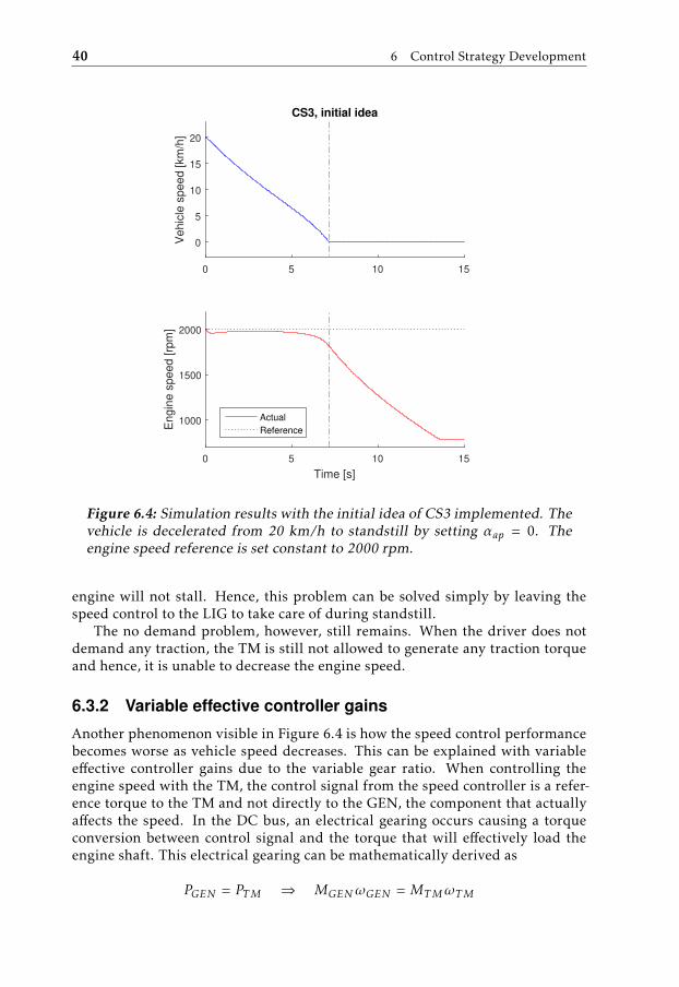
6.3.1 Initial idea

CS3 according to this initial idea is implemented in Simulink™ and a vehicledeceleration from 20 km/h to 0 km/h is simulated, with αap = 0 and a constantengine speed reference of 2000 rpm. The results are presented in Figure 6.4.

As seen in the figure, the same standstill problem as with CS2 is still presentin CS3 but now with engine speed instead of voltage; when the vehicle speedreaches zero, the engine speed drops as a consequence of the ICE generating anegative torque due to friction and pump losses and the TM is not able to keepit up as it lacks kinetic energy to do so. However, since the ECU has a low idlegovernor that kicks in when the speed drops below the low idle setpoint, the


0 5 10 15

0

5

10

15

20

Ve

hic

le s

pe

ed

[km

/h]

CS3, initial idea

0 5 10 15

Time [s]

1000

1500

2000

En

gin

e s

pe

ed

[rp

m]

Actual

Reference

Figure 6.4: Simulation results with the initial idea of CS3 implemented. Thevehicle is decelerated from 20 km/h to standstill by setting αap = 0. Theengine speed reference is set constant to 2000 rpm.

engine will not stall. Hence, this problem can be solved simply by leaving thespeed control to the LIG to take care of during standstill.

The no demand problem, however, still remains. When the driver does notdemand any traction, the TM is still not allowed to generate any traction torqueand hence, it is unable to decrease the engine speed.

6.3.2 Variable effective controller gains

Another phenomenon visible in Figure 6.4 is how the speed control performancebecomes worse as vehicle speed decreases. This can be explained with variableeffective controller gains due to the variable gear ratio. When controlling theengine speed with the TM, the control signal from the speed controller is a refer-ence torque to the TM and not directly to the GEN, the component that actuallyaffects the speed. In the DC bus, an electrical gearing occurs causing a torqueconversion between control signal and the torque that will effectively load theengine shaft. This electrical gearing can be mathematically derived as

PGEN = PTM ⇒ MGENωGEN = MTMωTM

6.4 Gear ratio compensated control signal 41

⇒ MTM =ωGENωTM

MGEN (6.1)

By defining the effective gear ratio as

ie ≡ωGENωTM

(6.2)

the following expressions are obtained:

MTM = ieMGEN ⇔ MGEN =1ieMTM (6.3)

The equation for the engine speed PI controller yields

u(t) = MTM = Kpe(t) + Ki

∫e(t) dt (6.4)

Combining Equations 6.3 and 6.4 yields

MGEN =1ie

Kpe(t) + Ki

∫e(t) dt

=Kpiee(t) +

Kiie

∫e(t) dt (6.5)

From this equation, it is clear that the controller gains will vary with the effec-tive gear ratio.

6.4 Gear ratio compensated control signal

The effect of variable controller gains can be counteracted by introducing controlsignal compensation using the effective gear ratio, that is

ucomp = ieuuncomp (6.6)

where ucomp and uuncomp are the compensated and uncompensated control sig-nals, respectively.

6.4.1 Deceleration from 20 km/h to standstill

Simulation results for a deceleration from 20 km/h to standstill after introduc-ing this compensation are shown in Figure 6.5. When comparing these resultsto the same deceleration without control signal compensation in Figure 6.4, itis evident that by introducing the compensation, speed control performance isconstant until the vehicle stops.


0 5 10 15

0

5

10

15

20

Ve

hic

le s

pee

d [km

/h]

CS3 with control signal compensation

0 5 10 15

Time [s]

1000

1500

2000

Engin

e s

peed [rp

m]

Actual

Reference

Figure 6.5: The same simulation as in Figure 6.4 is run, but with the controlsignal compensated for the varying effective gear ratio.

6.4.2 Full drive cycle

In Figure 6.6, the full drive cycle is simulated with control signal compensationimplemented and a constant speed reference of 2300 rpm. The driver demand isinterpreted into a demanded power simply as Pdem = αapPmax,nom.

One major problem is obvious: the TM never delivers the full demandedpower. This can be explained with the driver interpretation not compensatingfriction and pump losses in the engine, causing the actual delivered power to belower than the demanded power.

6.4 Gear ratio compensated control signal 43

0 10 20 30 40 50 60 70

0

50

100

150

200

Pow

er [k

W]

ICE and TM power

ICE

TM

Demand

0 10 20 30 40 50 60 70

0

50

100

150

200

Pow

er [k

W]

Power demands

Driver

AUX

PAR

0 10 20 30 40 50 60 70

1000

1500

2000

2500

Spe

ed [r

pm]

Engine speed

ActualReference

0 10 20 30 40 50 60 70

Time [s]

0

10

20

30

Spe

ed [k

m/h

]

Vehicle speed

Figure 6.6: Simulation results for the full fictive drive cycle with CS3 withcontrol signal compensation implemented.


6.5 Friction and pump loss compensation

Since the requested torque from the engine is an indicated torque, the actualbraking torque on the shaft is lower due to friction and pump losses. In orderto make the engine produce full power at maximum accelerator pedal position,these losses have to be compensated for. One way of doing this is by approximat-ing the losses and offset the ICE torque reference with this value, that is

Mice,ref =Pdemωice

+ Mloss(ωice) (6.7)

In this way, the engine would produce around 0 kW braking power at αap = 0and around Pmax at αap = 1.

6.5.1 Engine braking

In order to spare the mechanical brakes and hence reduce maintenance costs,engine braking is a desired feature. One drawback with friction compensationin the manner described above is that engine braking will be disabled by design.This can be explained with the following example.

Imagine a case when vveh > 0 and αap = 0. The desired behavior is that the TMregenerates power into the DC bus and consequently brakes the vehicle. Powerregeneration from the TM, which is the speed controlling unit, occurs when theengine speed is lower than the reference. If engine losses are not compensated,αap = 0 will imply a negative braking torque from the ICE. This torque willdecelerate the shaft, which the TM will try to compensate through feeding powerback through the powertrain and effectively engine braking the vehicle.

If, on the other hand, engine losses are compensated for, αap = 0 will implyaround zero net engine torque and consequently not cause shaft deceleration.Engine braking will thus not occur.

One possible approach to compensate the losses while still preserving theengine braking capability is to use a multiplication compensation factor in thedriver interpretation instead of adding a compensation offset to the ICE refer-ence torque. By approximating the losses at maximum engine speed and addingthis to maximum engine power, a compensation factor can be formed as

Pcomp = αap(Pmax + Pf ric(ωmax)) = αapPmax

(Pf ric(ωmax)

Pmax+ 1

)(6.8)

This way, αap = 1 will cause maximum engine power to be produced, whileαap = 0 will still imply a negative braking torque and thus engine braking.

Figure 6.7 shows the simulation results from the full drive cycle with frictioncompensated driver interpretation. As seen in this figure, the powertrain doesdeliver the full demanded power at αap = 1, but produces lower-than-requestedpowers for lower αap. This can be explained with the way the friction compensa-

tion is achieved. In Equation 6.8, the termPf ric(ωmax)

Pmaxestimates the ratio between

friction power and maximum power at maximum speed in order to reach full

6.5 Friction and pump loss compensation 45

power at full driver demand. At lower loads this ratio is typically bigger andhence, the compensation is not sufficient (clearly visible at 5-10 s when αap = 0.1but still no traction power is delivered). This is a drawback with the selected losscompensation technique. However, this problem is less significant with a moresophisticated engine speed reference selection technique implemented (keepingthe engine speed reference at a constant high level as in this simulation is notvery rational), which will be evident in later sections.

0 10 20 30 40 50 60 70

0

50

100

150

200

Pow

er [k

W]

ICE and TM power

ICE

TM

Demand

0 10 20 30 40 50 60 70

0

50

100

150

200

Pow

er [k

W]

Power demands

Driver

AUX

PAR

0 10 20 30 40 50 60 70

1000

1500

2000

2500

Spe

ed [r

pm]

Engine speed

ActualReference

0 10 20 30 40 50 60 70

Time [s]

0

10

20

30

Spe

ed [k

m/h

]

Vehicle speed

Figure 6.7: Driver interpretation using friction compensation factor.


6.6 Speed reference selection

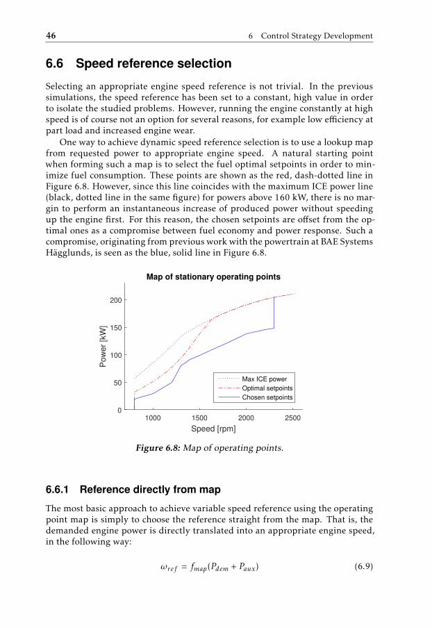
Selecting an appropriate engine speed reference is not trivial. In the previoussimulations, the speed reference has been set to a constant, high value in orderto isolate the studied problems. However, running the engine constantly at highspeed is of course not an option for several reasons, for example low efficiency atpart load and increased engine wear.

One way to achieve dynamic speed reference selection is to use a lookup mapfrom requested power to appropriate engine speed. A natural starting pointwhen forming such a map is to select the fuel optimal setpoints in order to min-imize fuel consumption. These points are shown as the red, dash-dotted line inFigure 6.8. However, since this line coincides with the maximum ICE power line(black, dotted line in the same figure) for powers above 160 kW, there is no mar-gin to perform an instantaneous increase of produced power without speedingup the engine first. For this reason, the chosen setpoints are offset from the op-timal ones as a compromise between fuel economy and power response. Such acompromise, originating from previous work with the powertrain at BAE SystemsHägglunds, is seen as the blue, solid line in Figure 6.8.

1000 1500 2000 2500

Speed [rpm]

0

50

100

150

200

Po

we

r [k

W]

Map of stationary operating points

Max ICE power

Optimal setpoints

Chosen setpoints

Figure 6.8: Map of operating points.

6.6.1 Reference directly from map

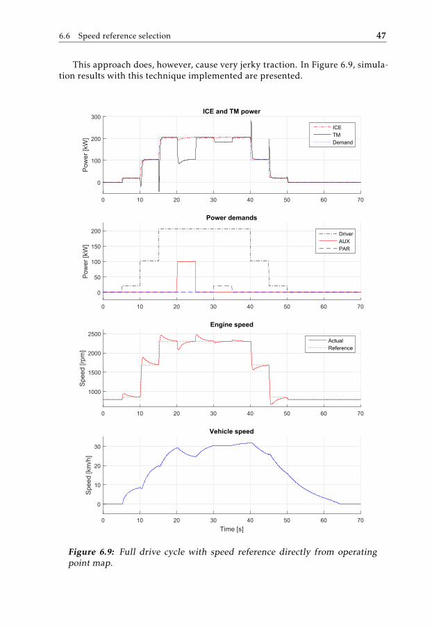
The most basic approach to achieve variable speed reference using the operatingpoint map is simply to choose the reference straight from the map. That is, thedemanded engine power is directly translated into an appropriate engine speed,in the following way:

ωref = fmap(Pdem + Paux) (6.9)

6.6 Speed reference selection 47

This approach does, however, cause very jerky traction. In Figure 6.9, simula-tion results with this technique implemented are presented.

0 10 20 30 40 50 60 70

0

100

200

300

Pow

er [k

W]

ICE and TM power

ICE

TM

Demand

0 10 20 30 40 50 60 70

0

50

100

150

200

Pow

er [k

W]

Power demands

Driver

AUX

PAR

0 10 20 30 40 50 60 70

1000

1500

2000

2500

Spe

ed [r

pm]

Engine speed

ActualReference

0 10 20 30 40 50 60 70

Time [s]

0

10

20

30

Spe

ed [k

m/h

]

Vehicle speed

Figure 6.9: Full drive cycle with speed reference directly from operatingpoint map.


As seen in this figure, when αap is increased (at 10 s and 15 s) TM powerdecreases initially and then increases to the desired level. This can also be seenin the vehicle speed plot where it is obvious that the vehicle decelerates beforestarting to accelerate. When αap is decreased (at 40 s, 45 s and 50 s) the oppositephenomenon occurs; when the accelerator pedal is let up, the traction quicklyincreases before decreasing. These jerks will be perceived as unintuitive to adriver (pushing down the accelerator pedal and the vehicle starts to decelerate)and can also be hazardous from a safety perspective and are thus unwanted.

However, Figure 6.9 also reveals a positive characteristic with the dynamicspeed reference selection technique; the delivered traction power now matchesthe desired power. This was not the case in Figure 6.7, which was explained

with the compensation factorPf ric(ωmax)

Pmaxin Equation 6.8 not being sufficient for

low loads while having a constantly high engine speed. At lower speeds the en-gine friction is also lower, making this compensation factor better match the trueratio between friction power at the current speed and maximum engine power.Sufficient compensation is therefore achieved.

6.6.2 Limited shaft acceleration torque

The jerks can be explained with the rapidly increasing speed reference. With in-creasing speed error, the torque needed to accelerate the shaft increases and thus,less torque is available for traction. One way to circumvent this phenomenon isto limit the torque used for shaft acceleration.

The torque produced by the ICE can be used for two purposes: shaft acceler-ation or further transmission through the powertrain, ultimately being used fortraction or external loads. This is visualized in Figure 6.10.

ICEMice

Jω

Mgen

Figure 6.10: Illustration of consumers of the ICE torque.

When choosing speed reference directly from the operating point map as inSection 6.6.1, the rate of change in engine speed is basically infinite during tran-sients. That is, more or less all engine torque is used to accelerate the shaft, caus-ing the jerky transients. In order to control the amount of torque used for shaftacceleration, the rate of change (i.e. the desired acceleration) can be limited. Thetorque needed for this acceleration can be expressed using Newton’s second lawfor rotation as

Macc = Jgensetωice (6.10)

where Macc is the shaft acceleration torque, Jgenset the moment of inertia of the

6.6 Speed reference selection 49

genset and ωice the shaft acceleration. By limiting the accelerating torque to acertain portion of the torque produced by the engine according to

Macc = βMice, 0 < β < 1 (6.11)

the balance between the two consumers can be controlled. Combining the twoequations above yields an expression for the corresponding speed reference rateof change limit as

ωice =βMice

Jgenset(6.12)

This limit is implemented in Simulink™ using a dynamic rate limiter, asshown in Figure 6.11. In addition to the rate limiter, a filter is added in orderto smoothen the reference signal and thereby further prevent bumpy traction.

Figure 6.11: Simulink™ implementation of rate limited speed reference se-lection.

Simulation results with this technique implemented are shown in Figure 6.12.As seen, the jerks are significantly reduced or even removed. Comparing thespeed reference curve in this case with speed reference selection directly fromthe map (Figure 6.9), it is also obvious that the reference transients are slower.


0 10 20 30 40 50 60 70

0

50

100

150

200

Pow

er [k

W]

ICE and TM power

ICE

TM

Demand

0 10 20 30 40 50 60 70

0

50

100

150

200

Pow

er [k

W]

Power demands

Driver

AUX

PAR

0 10 20 30 40 50 60 70

1000

1500

2000

2500

Spe

ed [r

pm]

Engine speed

ActualReference

0 10 20 30 40 50 60 70

Time [s]

0

10

20

30

Spe

ed [k

m/h

]

Vehicle speed

Figure 6.12: Simulation results after implementing the rate limited speedreference selection.

6.7 Traction power limit with ICE torque reduction 51

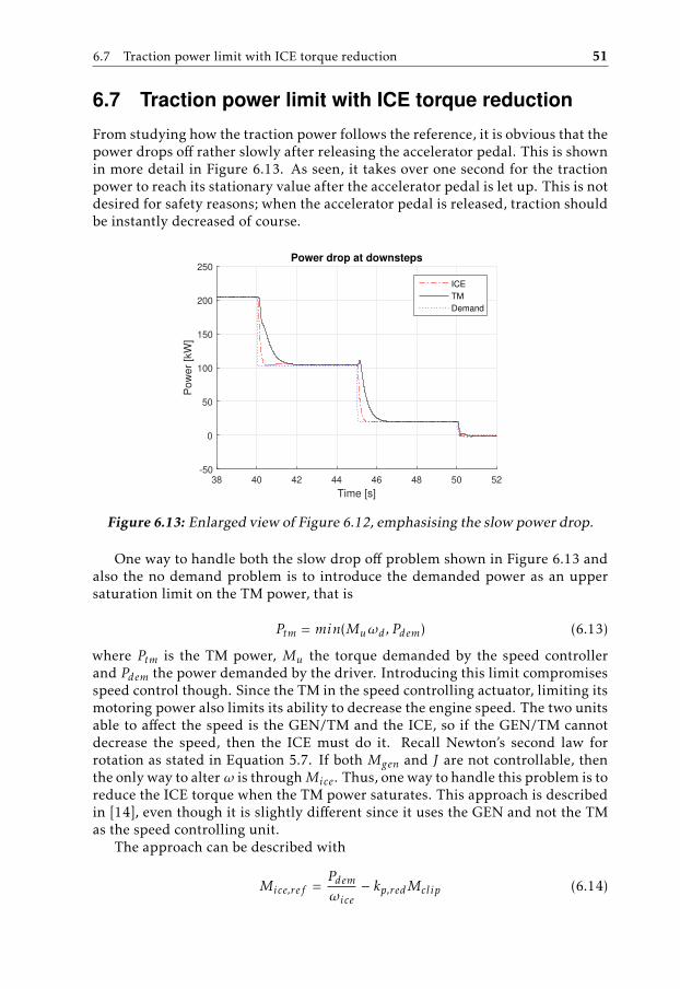
6.7 Traction power limit with ICE torque reduction

From studying how the traction power follows the reference, it is obvious that thepower drops off rather slowly after releasing the accelerator pedal. This is shownin more detail in Figure 6.13. As seen, it takes over one second for the tractionpower to reach its stationary value after the accelerator pedal is let up. This is notdesired for safety reasons; when the accelerator pedal is released, traction shouldbe instantly decreased of course.

38 40 42 44 46 48 50 52

Time [s]

-50

0

50

100

150

200

250

Po

we

r [k

W]

Power drop at downsteps

ICE

TM

Demand

Figure 6.13: Enlarged view of Figure 6.12, emphasising the slow power drop.

One way to handle both the slow drop off problem shown in Figure 6.13 andalso the no demand problem is to introduce the demanded power as an uppersaturation limit on the TM power, that is

Ptm = min(Muωd , Pdem) (6.13)

where Ptm is the TM power, Mu the torque demanded by the speed controllerand Pdem the power demanded by the driver. Introducing this limit compromisesspeed control though. Since the TM in the speed controlling actuator, limiting itsmotoring power also limits its ability to decrease the engine speed. The two unitsable to affect the speed is the GEN/TM and the ICE, so if the GEN/TM cannotdecrease the speed, then the ICE must do it. Recall Newton’s second law forrotation as stated in Equation 5.7. If both Mgen and J are not controllable, thenthe only way to alterω is throughMice. Thus, one way to handle this problem is toreduce the ICE torque when the TM power saturates. This approach is describedin [14], even though it is slightly different since it uses the GEN and not the TMas the speed controlling unit.

The approach can be described with

Mice,ref =Pdemωice

− kp,redMclip (6.14)


Mclip =

Mu −Msat , if Mu −Msat > 00, otherwise

(6.15)

Msat =Pdemωd

(6.16)

Simulation results with this technique implemented are presented in Figures6.14 (detailed view) and 6.15 (full drive cycle). With this approach, the deliveredpower strictly follows the demanded power at the downsteps. It is also obvioushow the ICE compensates by reducing the power when the TM power is clipped.

38 40 42 44 46 48 50 52

Time [s]

-50

0

50

100

150

200

250

Pow

er

[kW

]

Power drop at downsteps

ICE

TM

Demand

Figure 6.14: Power drop with TM power limit and ICE torque reductionimplemented.

6.7 Traction power limit with ICE torque reduction 53

0 10 20 30 40 50 60 70

0

50

100

150

200

Pow

er [k

W]

ICE and TM power

ICE

TM

Demand

0 10 20 30 40 50 60 70

0

50

100

150

200

Pow

er [k

W]

Power demands

Driver

AUX

PAR

0 10 20 30 40 50 60 70

1000

1500

2000

2500

Spe

ed [r

pm]

Engine speed

ActualReference

0 10 20 30 40 50 60 70

Time [s]

0

10

20

30

Spe

ed [k

m/h

]

Vehicle speed

Figure 6.15: Simulation results when having the maximum TM limit andICE torque reduction implemented.


6.8 Conditional idle speed setting

As visible in Figure 6.15, the vehicle does not engine brake when the acceleratorpedal is released. This is obvious from the ICE power being zero at αap = 0, whenthe desired behavior is Pice < 0.

This can be explained using the LIG. In the simulation run in Figure 6.15, thelow idle speed setpoint is 800 rpm. Thus, when the speed reference selectionalgorithm chooses the same 800 rpm as reference for the speed controller and thespeed falls below this point, the LIG will counteract this speed error instead ofthe regular speed controller doing it. Consequently, no engine braking will occur.

In order to circumvent this problem, the LIG speed setpoint can be offsetusing a deadband when the vehicle is moving, according to

ωref ,LIG =

ωref ,LIG,des − ωdb,LIG, if vveh > 0ωref ,LIG,des, otherwise

(6.17)

where ωref ,LIG is the effective speed reference to the LIG, ωref ,LIG,des the desiredsetpoint and ωdb,LIG the deadband.

Simulation results with this technique implemented and a deadband of 200rpm are presented in Figures 6.16 (detailed view) and 6.17 (full drive cycle). Asseen in these results, the engine consumes power when vveh > 0 and αap = 0 (i.e.between 50 s and 60 s), which is visible both in the power graphs and from com-paring the vehicle deceleration in this case with the case in Figure 6.15. Withoutthe conditional idle speed setting, a deceleration from 15 km/h to standstill takesapproximately 14 s, compared to 11 s in this case.

However the braking power the engine consumes is very low, just around2.5 kW. This is due to the low engine speed during braking which implies lowengine friction. If a higher speed reference was retained throughout the brakingprocedure, the increased friction would lead to more powerful engine braking.

48 50 52 54 56 58 60 62

Time [s]

-10

-5

0

5

10

15

20

25

Pow

er

[kW

]

Engine braking, detailed view

ICE

TM

Demand

Figure 6.16: Detailed view of Figure 6.17, emphasizing that the conditionalidle speed setpoint technique enables engine braking.

6.8 Conditional idle speed setting 55

0 10 20 30 40 50 60 70

0

50

100

150

200P

ower

[kW

]

ICE and TM power

ICE

TM

Demand

0 10 20 30 40 50 60 70

0

50

100

150

200

Pow

er [k

W]

Power demands

Driver

AUX

PAR

0 10 20 30 40 50 60 70

1000

1500

2000

2500

Spe

ed [r

pm]

Engine speed

ActualReference

0 10 20 30 40 50 60 70

Time [s]

0

10

20

30

Spe

ed [k

m/h

]

Vehicle speed

Figure 6.17: Simulation results with the conditional idle speed setpoint tech-nique implemented.


6.9 Infinite torque gain

Refer to Equation 6.2 describing the effective gear ratio. With decreasing vehiclespeed (and thus TM speed), the effective gear ratio increases. When the speedapproaches zero, the gear ratio grows to infinity, that is

limωTM→0+

ie = limωTM→0+

ωGENωTM

= ∞ (6.18)

An infinite effective gear ratio implies infinite gain from ICE torque to TMtorque. In other words, when the vehicle stands still and the driver just slightlytouches the accelerator pedal, the TM will initially deliver maximum torque. Thisis confirmed in simulation, which is shown in Figure 6.18 where the torque curvefrom the simulation presented in Figure 6.17 is shown. As visible, the torquequickly peaks at 5 s, even though the driver only requests 10% traction power.

0 10 20 30 40 50 60 70

Time [s]

-500

0

500

1000

1500

TM

torq

ue [N

m]

Torque peak at takeoff

Figure 6.18: TM torque peak at takeoff, due to infinite effective gear ratio.

6.9.1 Takeoff strategy

To handle the effect of infinite effective gear ratio, a takeoff strategy is necessary.Otherwise, driving at low speeds will be highly difficult. Several possible takeofftechniques are identified.

• Uncompensated control signalThe purpose of the control signal compensation described in Section 6.4 isto ensure constant speed control performance independent of vehicle speed.This comes with the disadvantage of high torques at low vehicle speeds,though. By accepting variable speed control performance, a smoother take-off can be achieved by using a non-compensated control signal.

• Mode switchUtilizing a pull control strategy at takeoff lets the driver directly control

6.9 Infinite torque gain 57

the actual traction torque which allows for more precise low speed driv-ing. Then switching mode to a push strategy at higher speeds enables theadvantages of this approach.

• TM torque limit at low speedsAn approach similar to the one described in Section 6.7 could be used; bylimiting the traction torque at low speeds and compensating the ICE torqueaccordingly, a softer takeoff could be realized.

Uncompensated control signal

The uncompensated control signal technique is implemented, and the simulationresults presented in Figure 6.19 for both compensated and uncompensated con-trol signal. As shown, the torque response when not using control signal compen-sation is much smoother than the compensated response. However, the smoothertakeoff torque comes at a cost of reduced speed control performance, which isobvious from comparing the engine speed plots for the two cases.

4 5 6 7 8

0

500

1000

1500

To

rqu

e [

Nm

]

Compensated control signal

Traction torque

4 5 6 7 8

Time [s]

500

1000

1500

Sp

ee

d [

rpm

]

Engine speed

Actual

Reference

(a)

4 5 6 7 8

0

500

1000

1500

To

rqu

e [

Nm

]

Uncompensated control signal

Traction torque

4 5 6 7 8

Time [s]

500

1000

1500

Sp

ee

d [

rpm

]

Engine speed

Actual

Reference

(b)

Figure 6.19: Traction torque and engine speed during takeoff for (a) com-pensated and (b) uncompensated control signals.

7Results

In this chapter, the final control strategy is presented together with the simula-tion results with this strategy implemented.

7.1 Final control strategy

The final control strategy works according to CS3 and makes use of the followingtechniques, as described in the previous chapter.

• Driver interpretation using engine loss compensation as described in Sec-tion 6.5

• Speed reference selection with limited shaft acceleration torque as describedin Section 6.6.2

• Traction power limit with ICE torque reduction according to Section 6.7

• Conditional idle speed setting as described in Section 6.8

• Uncompensated speed control signal as takeoff strategy as explained in Sec-tion 6.9.1

A block diagram of this strategy is presented in Figure 7.1.

7.1.1 Parameters

With this strategy, there are four strategy-specific tuning parameters.

• Proportion of demanded torque that should be allowed for shaft accelera-tion, β

59

60 7 Results

• Time constant for the speed reference low-pass filter

• Proportional reduction factor for clipped TM torque, kp,red

• Deadband for the conditional idle speed setpoint, ωdb

Additionally, the parameters for the speed controller in the PCM and the voltagecontroller in the GCU have to be tuned.

Traction powerlimit

Speed reference selection

ECU

Driver interpretation

GCU

ICE GEN TM

Uref

U control

+-

ω control

+-

ωref,lim

Mice,ref

αap

MTM,ref

× +

Pmax,nom Ploss(ωmax)

÷ ωice

+ Paux

min

Operatingpoint map Rate

limiter

÷

Jgenset

max

LIG

Low-pass filter

Pdem

ωref

Mdem÷

ωd

max

1

+-

max

0

β

kp,redMclip

Conditional idle setpoint

ωd

↑ PCM

ωidle

+-

ωmax

Figure 7.1: Block diagram of the final control strategy. Logic above the red,dash-dotted line is implemented in the PCM and logic below is realized inthe subcomponent control units. Note that necessary integrator anti-windupfeatures in the speed controller are omitted in this diagram. Furthermore,the max(ωd , 1) selector on the very right in the figure is added in order toprevent division by zero at standstill.

7.2 Simulation results 61

7.2 Simulation results

Simulation results from the three following cases are presented.

• Fictive drive cycle with full ICE performance

• Fictive drive cycle with ICE performance reduced by 30%

• Real drive cycle with full ICE performance

These results are presented objectively in this section, and are then discussed inthe next chapter.

62 7 Results

7.2.1 Fictive drive cycle, 100% ICE performance

0 10 20 30 40 50 60 70

0

50

100

150

200

Pow

er [k

W]

ICE and TM power

ICE

TM

Demand

ICE max

0 10 20 30 40 50 60 70

0

50

100

150

200

Pow

er [k

W]

Power demands

Driver

AUX

PAR

0 10 20 30 40 50 60 70

1000

1500

2000

2500

Spe

ed [r

pm]

Engine speed

ActualReference

0 10 20 30 40 50 60 70

Time [s]

0

10

20

30

Spe

ed [k

m/h

]

Vehicle speed

Figure 7.2: The final control strategy running the fictive drive cycle with fullICE performance.

7.2 Simulation results 63

7.2.2 Fictive drive cycle, 70% ICE performance

0 10 20 30 40 50 60 70

0

50

100

150

200

Pow

er [k

W]

ICE and TM power

ICE

TM

Demand

ICE max

0 10 20 30 40 50 60 70

0

50

100

150

200

Pow

er [k

W]

Power demands

Driver

AUX

PAR

0 10 20 30 40 50 60 70

1000

1500

2000

2500

Spe

ed [r

pm]

Engine speed

ActualReference

0 10 20 30 40 50 60 70

Time [s]

0

10

20

30

Spe

ed [k

m/h

]

Vehicle speed

Figure 7.3: The final control strategy running the fictive drive cycle with30% reduced engine performance.

64 7 Results

7.2.3 Real drive cycle

0 50 100 150 200 250

0

50

100

150

200

Pow

er [k

W]

ICE and TM power

ICE

TM

Demand

0 50 100 150 200 250

0

50

100

150

200

Pow

er [k

W]

Power demands

Driver

AUX

PAR

0 50 100 150 200 250

1000

1500

2000

2500

Spe

ed [r

pm]

Engine speed

ActualReference

0 50 100 150 200 250

Time [s]

0

10

20

30

Spe

ed [k

m/h

]

Vehicle speed

Figure 7.4: The final control strategy running the real drive cycle.

8Discussion

8.1 Results

In this section, the results from the previous chapter are discussed. First of all,from studying Figure 7.3 it is clear that the developed strategy solves the origi-nal maximum engine power utilization problem; when the driver demands morepower than available from the engine, maximum available power is delivered inline with the desired behavior. However, when comparing these results to theones presented in Figure 7.2 when the full engine power is available, it is noticedthat the introduced power reduction causes bumpy traction (occurring during thetransient at 15-16 s). This speaks for the basic speed reference selection strategyused not being robust enough to handle changing engine performance. Hence, amore sophisticated algorithm is needed in order to prevent these bumps.

8.1.1 Jerks during real drive cycle

In Figure 7.4, the results from the final strategy running the real drive cycle areshown. As seen, there are still some traction jerks occuring, even though a speedreference selection strategy aimed to prevent this is used. In Figure 8.1, detailedplots from the final strategy running the real drive cycle are shown. In these plots,three obvious occurrences of jerky traction are present at 46 s, 212 s and 222 s.All these jerks have in common that they occur when the AUX load (dashed, blackline) quickly increases. This is reasonable since the AUX loads occur instantly andstart to consume power from the DC bus, faster than the ICE can compensate theload by increasing the produced power. Hence, less power will be available fortraction initially and a jerk will occur.

This behavior might be acceptable to the driver, though. When starting to con-sume power with an external load, for example using the hydraulics, it is rather

65

66 8 Discussion

intuitive that traction power shortly decreases to give room for the introducedload. Thus, the severity of this issue is maybe not the highest.

35 40 45 50 55 60 65

Time [s]

0

50

100

150

200

Pow

er [k

W]

35 s - 65 s

200 205 210 215 220 225 230

Time [s]

0

50

100

150

200

200 s - 230 s

Demand

TM

AUX

Figure 8.1: Detailed plots from the simulation presented in Figure 7.4 em-phasizing three occurrences with jerky traction (46 s, 212 s and 222 s).

8.1.2 Natural priority handling

In the results, it is seen that the push strategy handles load priority in a naturalway. As stated in Chapter 1, the requirement is that external loads should takeprecedence over traction when they occur. From studying Figures 7.2 and 7.3 at20 s and 30 s when AUX and PAR loads appear while maximum traction power isbeing delivered, it is seen that traction power is naturally decreased, giving roomfor the external loads. This happens without having any priority-specific logicimplemented, which is seen as an advantage with this approach.

8.1.3 Uncertain applicability of real drive cycle signals

The recorded signals used as the real drive cycle are recorded on a vehicle whichuses a control strategy based on a torque request from the driver. In the devel-oped strategy on the other hand, the driver demand is interpreted as a desiredpower. This difference may jeopardize the applicability of the recorded driver sig-nals on the studied case since it is highly probable that the driver would behavedifferently in the two cases. For example, assume the driver desires a constant ac-celeration of the vehicle (i.e. a constant traction torque). In the case with a torquebased request, the driver would simply keep the accelerator pedal at a constantposition. However in the case with a power based request, a constant acceleratorpedal position would imply constant power and hence a continuously decreasingtraction torque due to the increasing vehicle speed. This is obvious in the torquecurve shown in Figure 6.18. For this reason, the driver would gradually increasethe accelerator pedal position in order to counteract this phenomenon, effectively

8.2 Modeling 67

working as a constant torque controller. It is thus conceivable that the acceleratorpedal position signal in a case when a power based driver interpretation is usedcould differ significantly from the torque based scenario, consequently makingthe applicability of the recorded drive cycle questionable.

8.2 Modeling

In this section, topics regarding the developed powertrain model are discussed.

8.2.1 Limited model validation

Since no recorded data from the studied powertrain has been available, no modelvalidation against real measurements has been possible. This is of course a signif-icant shortcoming in the work, limiting the credibility in the conclusions drawn.However, since the studied topic of the thesis is conceptual control strategies andgeneral characteristics rather than how the actual powertrain performs, the con-clusions are still regarded trustworthy.

As data from the real powertrain becomes available in the future, validatingand improving the model as necessary is suggested as prospective work.

8.2.2 Simplified component models

Many assumptions and simplifications have been made throughout the model-ing work. Two components that have been greatly simplified are the electric ma-chines (generator and traction motor), which are modeled as first-order systems.This simplification is motivated with the fact that the dynamics of the electricmachines are considerably faster than the dynamics of the ICE, which makes theICE the limiting component. If this simplification would be well off reality, it isconceivable that the real powertrain would behave significantly differently thanthe modeled one and that other, undiscovered phenomena would occur.

Furthermore, an aspect that has not been taken into consideration is the lossesin the power electronics. Since these losses are not modeled, the inverters are ef-fectively assumed to be loss-free. Having a small portion of the power dissipatingin these components would of course affect the powertrain performance, but it isquestionable whether it would alter the principal behavior of the powertrain ornot. Also, since a parasitic load connected to the DC bus is modeled, this dis-turbance can be seen as rather equivalent to the inverter losses except for themagnitude of the power.

68 8 Discussion

8.3 General discussion

This section discusses general aspects of the control strategy development work.

8.3.1 Speed control dynamics affecting traction

When the established pull strategy is used, the driver is in direct control of thetraction torque, while engine speed control is achieved by a controller. In thisway, the dynamics from the speed control (for example sudden torque transients)affect the ICE and not the TM. This will be noticed by the driver only aurally asvariances in engine speed, while traction typically remains unaffected.

When using the push approach, however, the driver is no longer in directcontrol of the traction, but controls it indirectly through the engine power, whilethe TM controls the engine speed (in the case of CS3). This causes traction, whichis the ultimate objective of the whole system, to be an effect of a control loopinstead of being directly driver initiated. The dynamics from the speed controlwill therefore affect the traction instead of the engine, which is disadvantageousfrom a drivability perspective.

The problem with traction jerks discussed above is a result from this character-istic. In order to achieve smooth traction using the push principle, a good enginespeed reference selection technique is needed.

8.3.2 Driver interpretation using traction torque

Throughout the thesis, the driver demand is interpreted as a requested enginepower. As a consequence, the traction torque will decrease with increasing vehi-cle speed for a constant accelerator pedal position. This is visible for example inFigure 6.18, where the sawtooth-like shape of the torque curve is an effect of thischaracteristic.

This approach is not the obvious solution though. An alternative techniqueis to interpret the driver demand as a requested traction torque, and then calcu-late which ICE torque this corresponds to. However, there is one major probleminvolved with this approach: at standstill, the effective gear ratio and thus thetorque gain from ICE torque to TM torque is infinite as shown in Equation 6.18,making it difficult to achieve the desired traction torque for low speeds. Still, thisproblem is already present with the power interpretation as implemented in thisthesis, speaking for a driver interpretation based on traction torque not beingmore difficult than the power-based counterpart.

8.3.3 CS1 with control loop migration

In CS3, the engine speed control loop is migrated to the PCM. This migrationenables greater control design freedom. In the established CS1, engine speedcontrol is achieved by the ECU. If this control loop was migrated to the PCM aswell, the traditional CS1 could possibly be improved. Such a migration wouldfor example enable the possibility to add a feed-forward part to the control loop,

8.3 General discussion 69

something that is not possible with todays established strategy. Adding a feed-forward part could make the ICE respond faster when a traction demand occursand hence improve the response of the whole powertrain.

8.3.4 Benefits of energy storage

As stated in the Delimitations section, adding an energy storage to the powertrainhas not been an option during this thesis. However, it has to be mentioned thatadding such a feature would enable at least two advantages.

• Reduced fuel consumption - Adding an energy storage would enable thepossibility to take care of regenerated energy during braking, to then utilizeit during accelerations. This could potentially lead to significant reductionsin fuel consumption, cutting both costs and environmental impact.

• Improved transient performance - Without energy storage the power pro-duced by the ICE has to go either to traction, external consumers or to in-creasing shaft speed or voltage. In a case when there is no external consump-tion and the shaft speed and voltage references are constant, all power fromthe ICE has to go to traction. In this way, any irregularity in ICE power (forexample due to turbo lag) will propagate to the TM. If an energy storagewould be present, power could be provided from this component in orderto achieve smoother transients.

• Increased braking capacity - In the studied powertrain, braking withoutusing the mechanical brakes is limited to engine braking, and even at themaximum speed of the engine, the engine braking power is only approxi-mately 29 kW. If energy storage was possible, the braking capacity couldbe significantly increased by charging the storage with regenerated powerfrom the TM. This would spare the mechanical brakes and thus reducemaintenance costs.

Additionally, adding this component would also make other control strategiespossible. For example, recall Figure 6.2 where the power paths through the DCbus are analyzed. If an energy storage was present, CS2 could possibly be feasiblesince the problems encountered at standstill and no traction demand could behandled with this energy storage.

9Conclusions & Future Work

9.1 Conclusions

In this section the conclusions drawn from the thesis are summarized. Theseconclusions are presented together with the questions in Section 1.3 in order toreconnect to the initial problem formulation.

How can a control system working according to the proposed strategy berealized?

The proposed control strategy in its original form (CS2) is not feasible due tothe inability to achieve voltage control using the TM when 1) the vehicle standsstill, and 2) the driver demands no traction. Tweaking CS2 to handle these cornercases is difficult in practice since both voltage and speed control are realized onsubcomponent level in the TCU and GCU respectively, greatly limiting the con-trol design possibilities. However, alternative approaches still working accordingto the push principle are possible, for example by migrating control loops fromthe subcomponent control units to the PCM.

In this thesis, a working push control strategy is developed and presented.This strategy proves that it is possible to successfully control a diesel-electricpowertrain according to the push principle.

Which advantages and disadvantages does the proposed control strategyposses?

The identified advantages and disadvantages with the push approach are listedbelow.

• Using the push control approach solves the original problem with max-imum utilization of the available engine power, potentially allowing for

71

72 9 Conclusions & Future Work

downsizing of the installed engine.

• A push control strategy naturally handles load prioritization in the casewhen external loads have higher priority than traction, without the need toimplement any priority-specific logic.

• Takeoff and slow speed driving are problematic by design due to the vary-ing effective gear ratio which grows to infinity when the vehicle speed ap-proaches zero. This implies that even the smallest possible increase in ICEtorque will cause the TM to generate maximum torque at standstill. Hence,a deliberate takeoff strategy is crucial in order to handle this characteristic.

• In the push principle the driver controls the ICE instead of the TM, whilethe TM controls the engine speed (in the case of the developed CS3). Thisapproach gives the driver only indirect control of the traction torque, andmakes dynamics from the speed control affect the traction. This mightcause bumpy acceleration of the vehicle and is thus disadvantageous from adrivability perspective. Furthermore, this puts high demands on the speedreference selection algorithm which plays a critical role in counteractingthis undesired bumpiness.

Are there other control strategies that are worth considering for thisapplication?

During the work, no other alternative control approaches have been identified.

9.2 Future work

With the developed control strategy, powertrain control according to the pushapproach can be realized. This brings the benefit of potential reduction in in-stalled engine size, which enables several advantages. Since some problematiccharacteristics have been identified with this approach, further work is neededin order to improve the developed strategy and make it practically applicable.Such prospective areas of improvement are presented below.

9.2.1 Speed reference selection algorithm

The speed reference selection algorithm is of major importance for achievingsmooth traction. In this thesis a rather basic algorithm is applied, so develop-ing a more sophisticated one could improve performance significantly. Below,some ideas for further improvement of this algorithm are presented.

• Achieve movement of the operating point in the engine map in a more opti-mal manner during transients, maybe as described in [16].

• Sustain a high engine speed reference during engine braking to maximizeengine braking power.

9.2 Future work 73

• Choose the proportion of produced ICE torque allowed for shaft accelera-tion β in a dynamic, more refined way.

• Instead of using an operating point map where the desired engine speedchanges continuously with requested power (as in this thesis), the enginespeed reference could be fixed in discrete intervals, imitating the gears ofa gearbox. It is conceivable that this technique could reduce the tractionbumpiness since speed reference changes, which are the main causes forthe bumps, would occur less often.

9.2.2 Takeoff strategy

Having a well-functioning takeoff strategy is important in order to enable satis-factory low speed driving. Three possible approaches have been identified in thethesis, of which only one is tested. It would be interesting to see a deeper analy-sis of this topic, both evaluating the identified approaches and generating other,more advanced concepts. One prospective takeoff technique that is consideredparticularly interesting is using the pull principle at low vehicle speeds, to thenperform a mode switch to the push principle when the speed increases.

9.2.3 Improved model validation

As no measurement data from the real powertrain has been available, the possi-bility to perform adequate validation of the developed model has been limited.Thus, it would be highly relevant to perform such validation as measurementsbecome available.

9.2.4 Extended fictive drive cycle

In the thesis, a considerably simplified drive cycle is used to evaluate the controlstrategy. Extending this drive cycle to incorporate more load cases (for exampleby introducing AUX and PAR loads at 0% and 50% traction power) could revealfurther characteristics of the strategy.

Bibliography

[1] SAE J1939 standard, accessed 2018-04-04. URL https://www.sae.org/standards/content/j1939_201308/. Cited on pages 8, 26, and 30.

[2] Stefano Barsali, Massimo Ceraolo, and Andrea Possenti. Techniques to con-trol the electricity generation in a series hybrid electrical vehicle. IEEETransactions on Energy Conversion, 17(2):260–266, 2002. Cited on page19.

[3] S. Chandra and M.M. Agarwal. Railway Engineering. Oxford UniversityPress, 2007. Cited on page 19.

[4] Linköping University Vehicular Systems division. Software, 2018. URLhttp://www.vehicular.isy.liu.se/Software/. Cited on page 15.

[5] Mehrdad Ehsani, Gao Yimin, Sebastien E. Gay, and Ali Emadi. ModernElectric, Hybrid Electric, and Fuel Cell Vehicles: Fundamentals, Theory andDesign. CRC Press LLC, 2005. Cited on page 19.

[6] Lars Eriksson and Lars Nielsen. Modeling and Control of Engines and Driv-elines. John Wiley & Sons, 2014. Cited on pages 21 and 25.

[7] R.D. Geertsma, R.R. Negenborn, K. Visser, and J.J. Hopman. Design andcontrol of hybrid power and propulsion systems for smart ships: A reviewof developments. Applied Energy, 194, 2017. Cited on page 20.

[8] Jan Fredrik Hansen and Frank Wendt. History and state of the art in commer-cial electric ship propulsion, integrated power systems, and future trends.Proceedings of the IEEE, 103(12), 2015. Cited on page 20.

[9] Jan Fredrik Hansen, Alf Kåre Ådnanes, and I. Fossen Thor. Mathematicalmodelling of diesel-electric propulsion systems for marine vessels. Mathe-matical and Computer Modelling of Dynamical Systems, 7(1), 2001. Citedon page 21.

[10] Amir Khajepour, Saber Fallah, and Avesta Goodarzi. Electric and hybridvehicles: technologies, modeling and control: a mechatronic approach. JohnWiley & Sons, 2014. Cited on page 19.

75

https://www.sae.org/standards/content/j1939_201308/

https://www.sae.org/standards/content/j1939_201308/

http://www.vehicular.isy.liu.se/Software/

76 Bibliography

[11] Werner Leonhard. Control of Electrical Drives. Springer-Verlag Berlin Hei-delberg, 2nd edition, 1996. Cited on page 9.

[12] Chris Mi, M. Abul Masrur, and David Wenzhong Gao. Hybrid Electric Ve-hicles: Principles and Applications with Practical Perspectives. John Wiley& Sons, 2011. Cited on page 19.

[13] V. Nezhadali, M. Sivertsson, and L. Eriksson. Turbocharger dynamics influ-ence on optimal control of diesel engine powered systems. SAE Interna-tional Journal of Engines, 7(1), 2014. Cited on page 20.

[14] M. Sivertsson and L. Eriksson. Optimal and real-time control potential ofa diesel electric powertrain. Proceedings of the 19th IFAC World Congress,Cape Town, South Africa, 2014. Cited on page 51.

[15] M. Sivertsson and L. Eriksson. Modeling for optimal control: A validateddiesel-electric powertrain model. SIMS2014 - 55th International Conferenceon Simulation and Modelling, Aalborg, Denmark, 2014. Cited on pages 15,21, 23, and 25.

[16] M. Sivertsson and L. Eriksson. Optimal transient control trajectories indiesel–electric systems—part i: Modeling, problem formulation, and engineproperties. Journal of Engineering for Gas Turbines and Power, 137(2), 2015.Cited on pages 21 and 72.

[17] M. Sivertsson and L. Eriksson. Optimal transient control trajectories indiesel–electric systems—part ii: Generator and energy storage effects. Jour-nal of Engineering for Gas Turbines and Power, 137(2), 2015. Cited on page21.

[18] Asgeir J. Sørensen and Øyvind N. Smogeli. Torque and power control of elec-trically driven marine propellers. Control Engineering Practice, 17, 2009.Cited on page 20.

[19] Stefan Östlund. Electrical Machines and Drives. KTH Electrical Machinesand Power Electronics, 2009. Cited on page 9.

[20] J. Wahlström and L. Eriksson. Modelling diesel engines with a variable-geometry turbocharger and exhaust gas recirculation by optimization ofmodel parameters for capturing non-linear system dynamics. Proceedingsof the Institution of Mechanical Engineers, Part D, Journal of AutomobileEngineering, 225(7), 2011. Cited on page 21.

Date post:	02-Jan-2022
Category:	Documents
Upload:	others
View:	0 times
Download:	0 times

Development of Push Control Strategy for Diesel-Electric ...

Documents