Page 1
Development of STATCOM based PI and Fuzzy
Voltage Controller for Self-Excited Induction
Generator
A thesis
submitted by
Sumit Singh
Roll no. 710EE2127
In the partial fulfilment of the requirements
for the award of the degree of
Bachelor of Technology
and
Master of Technology
(DUAL DEGREE)
Under the Supervision of
Prof. K. B. Mohanty
Department of Electrical Engineering
National Institute of Technology
Rourkela
Page 2
i
Department of Electrical Engineering
National Institute of Technology
Rourkela
CERTIFICATE
This is to certify that the thesis entitled “Development of
STATCOM based PI and Fuzzy Voltage Controller for Self-
Excited Induction Generator” being submitted by Sumit Singh
(710EE2127), for the award of the degree of Bachelor of Technology
and Master of Technology (Dual Degree) in Electrical Engineering,
is a bona fide research work carried out by him in the Department
of Electrical Engineering, National Institute of Technology,
Rourkela under my supervision and guidance
The research reports and the results embodied in this thesis have not
been submitted in parts or full to any other University or Institute
for award of any other degree.
Prof. Kanungo Barada Mohanty
Date: Department of Electrical Engineering Place: Rourkela NIT Rourkela, Odisha
Page 3
ii
ACKNOWLEDGEMENT
I express my deepest gratitude and sincere thanks to my supervisor Prof. Kanungo Barada
Mohanty for his constant motivation and support during the course of my research work.
Working with him has opened up a new horizon of state of art knowledge. His continuous
monitoring, valuable guidance and input, have been always the source of inspiration and
courage which are the driving forces to complete my work. My heartfelt thanks and deep
gratitude to Mrs. Jyotirmayee Dalei, who have equally given me valuable guidance, advice,
inspired me and patiently helped me in my work. I am overwhelmed with her immeasurable
valuable input and help received during my research work.
I would like to earnestly extend my deepest gratitude to Ms. Priyanka Priyadarshini, for
constantly motivating me and inspiring me with her valuable suggestions. My deepest love,
appreciation and indebtedness go to my parents for their wholehearted support, encouragement
and time sharing. Last but not the least I would like to thanks the GOD for their blessing to
help me raised my academic level to this stage.
Sumit Singh
710EE2127
Page 4
iii
Abstract
With growing demand of electrical energy and limited availability of fossil fuels has led to the
use of non-conventional sources (like Wind, Solar, Tidal etc.) which are abundant in nature
and pollutant free. The brushless generation using Induction generator with excitation capacitor
known as self-excited induction generators driven by constant speed prime movers are
becoming more popular because of its low cost, ruggedness, low maintenance and no need of
DC excitation system since last two decades. Moreover, these generators can also be operate
as stand-alone system to provide electricity to isolated rural areas where transmission of power
through grid is difficult and uneconomical. However the fundamental problem associated with
such generation scheme are poor voltage regulation under varying load. In order to regulate its
terminal voltage with varying load the active and reactive power levels at PCC (point of
common coupling) have to be maintained constant.
The active and reactive power level are regulated by using modern power electronic converters.
But survey shows that existing controllers are either difficult to implement or uneconomical or
designed for particular load only. This thesis is intended to develop a STATCOM based voltage
controller using PI controller for SEIG feeding both linear and non-linear loads driven by
constant speed prime mover. The PI controller based voltage regulator has poor dynamic
response hence a Fuzzy controller based voltage regulator using STATCOM is also developed.
The advantages of using Fuzzy Controller over PI Controller for development of STACOM
based voltage regulator for SEIG is investigated.
Page 5
iv
Table of Contents
CERTIFICATE ......................................................................................................................... i
ACKNOWLEDGEMENT ....................................................................................................... ii
Abstract ................................................................................................................................... iii
List of Figures ......................................................................................................................... vii
List of Symbols ......................................................................................................................... x
Chapter-1 .................................................................................................................................. 1
Introduction .............................................................................................................................. 1
1.1 General ............................................................................................................................ 1
1.2 Literature survey ............................................................................................................ 2
1.3 Motivation and Objective .............................................................................................. 4
1.4 Thesis Layout .................................................................................................................. 5
Chapter-2 .................................................................................................................................. 6
DESIGN OF DYNAMIC MODEL OF SELF-EXCITED INDUCTION GENERATOR
DRIVEN BY CONSTANT SPEED PRIME MOVER ......................................................... 6
2.1 General ............................................................................................................................ 6
2.2 Modelling of SEIG .......................................................................................................... 6
2.2.1 Excitation Model .................................................................................................... 10
2.2.2 Load Modelling ...................................................................................................... 11
2.3 Voltage build-up process in SEIG .............................................................................. 11
2.4 Simulation of SEIG driven by constant speed prime mover in
MATLAB/SIMULINK ...................................................................................................... 12
2.5 Results and Discussion ................................................................................................. 15
2.5.1 Self-excitation process ........................................................................................... 15
2.5.2 Insertion of Load ................................................................................................... 16
2.5.3 Loss of Excitation due to heavy-load ................................................................... 18
2.5.4 Step change in prime mover speed ....................................................................... 19
2.6 Conclusion ..................................................................................................................... 20
Chapter-3 ................................................................................................................................ 21
MODELLING OF STATCOM BASED VOLTAGE CONTROLLER FOR SEIG
DRIVEN BY CONSTANT SPEED PRIME MOVER USING CONVENTIONAL PI
CONTROLLER ..................................................................................................................... 21
3.1 Introduction .................................................................................................................. 21
3.2 About STATCOM ........................................................................................................ 21
Page 6
v
3.2.1 Control scheme for SEIG ...................................................................................... 23
3.3 Modelling of SEIG-STATCOM .................................................................................. 25
3.3.1 Modelling of control scheme involved ................................................................. 25
3.3.2 Modelling of STATCOM ...................................................................................... 27
3.3.3 Modelling of SEIG ................................................................................................. 28
3.3.4 AC Line Voltage at PCC (Point of Common Coupling) .................................... 29
3.3.5 Linear Load Modelling ......................................................................................... 30
3.3.6 Modelling of Non-linear load ................................................................................ 30
3.4 Simulation of SEIG-STACOM with PI Control in MATLAB/SIMULINK ........... 30
3.5 Result and Discussion .................................................................................................. 32
3.5.1 Voltage Build-up and Switch on STATCOM...................................................... 32
3.5.2 Connection of Load and Switching of Gate Pulses ............................................. 34
3.5.3 Performance of SEIG-STATCOM with PI Controller feeding Resistive Load
.......................................................................................................................................... 37
3.5.4 Performance of SEIG-STATCOM with PI Controller feeding R-L Load ....... 40
3.5.5 Performance of SEIG-STATCOM with PI Controller feeding Non-linear load
(Three Phase Diode Rectifier with Resistive load) ...................................................... 43
3.6 Conclusion ..................................................................................................................... 46
Chapter-4 ................................................................................................................................ 47
MODELLING OF STATCOM BASED FUZZY VOLTAGE CONTROLLER FOR
SEIG DRIVEN BY CONSTANT SPEED PRIME MOVER ............................................. 47
4.1 General .......................................................................................................................... 47
4.2 Basic of Fuzzy Controller ............................................................................................ 47
4.3 Modelling of STATCOM with Fuzzy Logic Controller ............................................ 49
4.4 Simulation of SEIG-STACOM with Fuzzy Logic Control in
MATLAB/SIMULINK ...................................................................................................... 52
4.5 Result and Discussion .................................................................................................. 52
4.5.1 Voltage build-up of SEIG, Connection of Load and Switching of Gate Pulses
for R Load ....................................................................................................................... 52
4.5.2 Performance of SEIG-STATCOM with Fuzzy Logic Control feeding R Load
.......................................................................................................................................... 55
4.5.3 Performance of SEIG-STATCOM with Fuzzy Logic Control feeding R-L
Load ................................................................................................................................. 58
4.5.4 Performance of SEIG-STATCOM with Fuzzy Logic Control feeding Non-
linear load (Three Phase Diode Rectifier with Resistive load) ................................... 61
4.6 Conclusion ..................................................................................................................... 65
Page 7
vi
Chapter-5 ................................................................................................................................ 66
MAIN CONCLUSION AND SCOPE FOR FUTURE WORK ......................................... 66
5.1 Main Conclusion ........................................................................................................... 66
5.2 Scope for future work .................................................................................................. 66
REFERENCES ....................................................................................................................... 68
Page 8
vii
List of Figures
Fig. 2.1 Schematic diagram of SEIG
Fig. 2.2 q-d axis diagram of SEIG
Fig. 2.3 Equivalent two phase machine
Fig. 2.4 Steady state circuit model of self-excited induction generator
Fig. 2.5 Dynamic d-q model of SEIG in Stationary reference frame
Fig. 2.6 Determination of Stable operation of SEIG
Fig. 2.7(a) Simulink model of SEIG in MATLAB
Fig. 2.7(b) Subsystem of d-q Induction generator model
Fig. 2.7(c) Subsystem of stator and rotor d-q axis current derivation
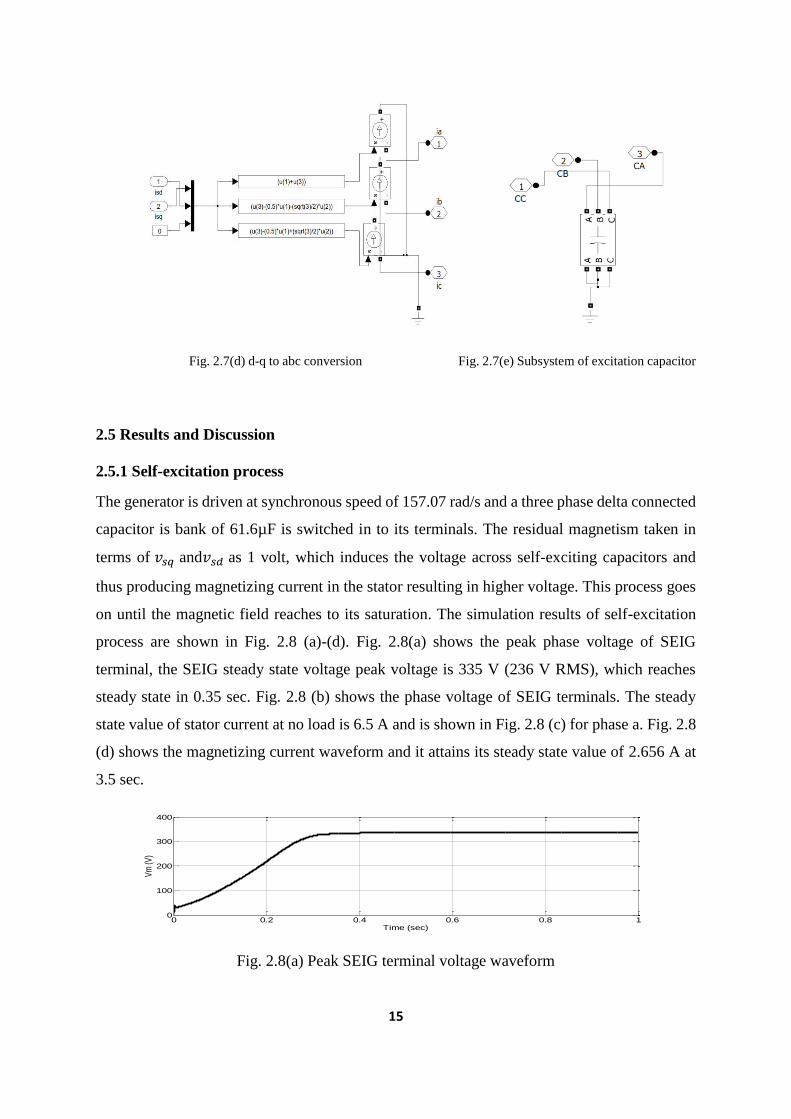
Fig. 2.7(d) d-q to abc conversion
Fig. 2.7(e) Subsystem of excitation capacitor
Fig. 2.8(a) Peak SEIG terminal voltage waveform
Fig. 2.8(b) Phase ‘a’ current of SEIG at no load
Fig. 2.8 (c) Waveform of SEIG terminal voltage
Fig. 2.8 (d) Magnetizing current waveform
Fig. 2.9(a) SEIG peak voltage Waveform
Fig. 2.9(b) Stator terminal phase voltage waveform
Fig. 2.9(c) Load current waveform
Fig. 2.9(d) Stator current Waveform
Fig. 2.9(e) Magnetizing current waveform
Fig. 2.10(a) SEIG peak voltage waveform
Page 9
viii
Fig. 2.10(b) SEIG terminal voltage (phase)
Fig. 2.10(c) Magnetizing current waveform
Fig. 2.11(a) SEIG peak voltage waveform
Fig. 2.11(b) Magnetizing current waveform
Fig. 2.12 Steady state waveform during voltage build-up
Fig. 3.1 1 (a) Schematic diagram of SEIG-STATCOM system, (b) Control scheme applied to
SEIG-STATCOM
Fig. 3.2 Three-phase diode rectifier with R-load
Fig. 3.3 Simulink diagram of SEIG-STATCOM
Fig. 3.4 Subsystem of Controller
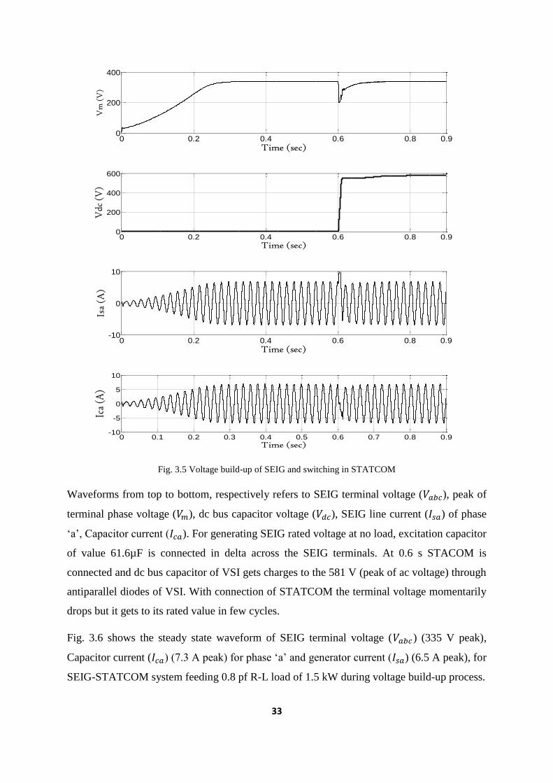
Fig. 3.5 Voltage build-up of SEIG and switching in STATCOM
Fig. 3.6 Steady state waveforms during voltage build-up process
Fig. 3.7 Performance of SEIG-STATCOM with PI controller feeding 0.8 pf R-L load of 1.5
kW (at 0.6 s STATCOM is connected, load is connected at 0.9 s and gate pulses given at 1.4s)
Fig. 3.8 Performance of SEIG-STATCOM system with PI controller supplying resistive load
(The load increased from 1.5 kW to 2.5 kW at 2.8 s and decrease to 1.5 kW at 3.5 s)
Fig. 3.9 Steady state waveform for SEIG-STATCOM system with PI controller feeding R load
of 1.5 kW
Fig. 3.10 Performance of SEIG-STATCOM system with PI controller feeding 0.8 pf R-L load
(Load is changed from 1.5 kW to 2.2 kW at 2.8 s and decrease to 1.5 kW at 3.5 s)
Fig. 3.11 Steady state waveform for SEIG-STATCOM system with PI controller feeding 0.8
pf R-L load of 2.5 kW
Fig. 3.12 Performance of SEIG-STATCOM system with PI controller feeding a non-linear load
(A three phase diode rectifier with resistive load change from 2 kW to 1.5 kW at 2.5 s)
Fig. 3.13 Steady state waveform for SEIG-STATCOM system with PI controller feeding three
phase diode rectifier with restive load of 2 kW
Page 10
ix
Fig. 4.1 Basic components of Fuzzy controller
Fig. 4.2 Fuzzy control scheme for dc bus voltage control
Fig. 4.3 Fuzzy control scheme for ac peak voltage control
Fig. 4.4 Performance characteristics of SEIG-STATCOM with Fuzzy Controller feeding R
load of 1.5 kW (at 0.6 s STATCOM is connected, load is connected at 0.95 s and gate pulses
given at 1.4 s)
Fig. 4.5 Steady state waveform for SEIG-STATCOM system with Fuzzy controller feeding R
load of 1.5 kW
Fig. 4.6 Performance characteristics of SEIG-STATCOM system with Fuzzy controller
supplying resistive load (Load is changed from 1.5 kW to 2.5 kW at 1.8 s and decrease to 1.5
kW at 2.3 s)
Fig. 4.7 Steady state waveform for SEIG-STATCOM system with Fuzzy controller feeding R
load of 2.5 kW
Fig. 4.8 Performance of SEIG-STATCOM with Fuzzy Controller feeding 0.8 pf R-L load
(Load is changed from 1.5 kW to 2.2 kW at 1.8 s and decrease to 1.5 kW at 2.2 s)
Fig. 4.9 Steady state waveforms of SEIG-STATCOM with Fuzzy Controller feeding 0.8 pf R-
L load of 1.5 kW
Fig. 4.10 Performance characteristics of SEIG-STATCOM system with Fuzzy controller
feeding diode rectifier with resistive load is decrease from 2 kW to 1.5 kW at 1.8 s and increase
from 1.5 kW to 2 kW at 2.2 s
Fig. 4.11 Steady state waveforms of SEIG-STATCOM with Fuzzy Controller feeding three
phase diode rectifier with resistive load of 2 kW
Fig. 4.12 DC bus capacitor voltage during switch on response
Page 11
x
List of Symbols
𝑣𝑞𝑠𝑠 , 𝑣𝑑𝑠
𝑠 Stator q and d axis voltage in stationary reference frame
𝑣𝑞𝑟𝑠 , 𝑣𝑑𝑟
𝑠 Rotor q and d axis voltage in stationary reference frame
𝑖𝑞𝑠𝑠 , 𝑖𝑑𝑠
𝑠 Stator q and d axis current in stationary reference frame
𝑖𝑞𝑟𝑠 , 𝑖𝑑𝑟
𝑠 Rotor q and d axis current in stationary reference frame
𝑟𝑠 Stator resistance of induction machine
𝑟𝑟 Rotor resistance of induction machine
𝜔𝑟 Speed of rotor
𝑙𝑠 Inductance of stator of induction machine
𝑙𝑟 Inductance of rotor of induction machine
M Magnetizing inductance
𝑇𝑒 Electromagnetic torque
𝑇𝑠ℎ𝑎𝑓𝑡 Shaft torque
𝐽 Moment of inertia of generator
𝑖𝑚 Magnetizing current
𝐶𝑒𝑞, 𝐶𝑒𝑑 Excitation capacitor values along q and d axis
𝑅𝐿, 𝐿𝐿 Load resistance and inductance
𝑉𝑚 Peak value of voltage
𝑢𝑎, 𝑢𝑏 , 𝑢𝑐 In-phase unit vectors
𝑤𝑎, 𝑤𝑏 , 𝑤𝑐 Quadrature unit vectors
Page 12
xi
𝑖𝑠𝑚𝑞∗ Peak quadrature supply current component along q axis
𝑖𝑠𝑚𝑑∗ Peak quadrature supply current component along d axis
𝑖𝑠𝑎𝑞∗ , 𝑖𝑠𝑏𝑞
∗ , 𝑖𝑠𝑐𝑞∗ Reference supply currents
𝑖𝑠𝑎, 𝑖𝑠𝑏 , 𝑎𝑛𝑑 𝑖𝑠𝑐 Source currents
𝑉𝑝𝑟𝑒𝑓 Reference ac voltage
𝑉𝑑𝑐𝑟𝑒𝑓 Reference ac voltage
𝑉𝑑𝑐 DC bus voltage
𝐼𝑠𝑎, 𝐼𝑠𝑏 , 𝐼𝑠𝑏 SEIG line currents
𝐼𝐿𝑜𝑎𝑑 𝑎𝑏𝑐 Three phase load current
𝑉𝑎𝑏𝑐 Three phase SEIG terminal voltage
𝐼𝑚𝑎, 𝐼𝑚𝑏 , 𝐼𝑚𝑐 Three phase STATCOM currents or compensating currents
𝑉𝑚 Magnitude of terminal voltage of SEIG
Page 13
1
Chapter-1
Introduction
1.1 General
With increasing demand for electrical power, more emphasis is given on the renewable source
of energy for producing electrical power. The depletion of conventional fuels has led to the use
of renewable sources of energy like solar, wind, biomass, tidal, etc. Of these, the wind energy
is found to be most suitable, clean, abundant and economical form of the non-conventional
sources.
Earlier Synchronous generators are used for power generation using wind energy. But their
application is limited as they cannot produce electricity at variable speed, require separate DC
excitation system and require more maintenance. But now the brushless generation using
Induction generator are more commonly used. The induction generator can be used either in
grid connected mode or in standalone mode as self-excited induction generators [2]-[10]. The
operation of induction generator as standalone system is gaining more attention, as they can
provide power to remote areas where it is difficult or uneconomical for power transmission line
to supply power. Thus the advantage of using induction generator are low cost, ruggedness,
low maintenance, simple operation, good dynamic response and no need of separate DC
excitation system.
The SEIG are proved to be best candidate for generating electricity from wind because they
don’t need external power supply for excitation and hence can be operate in remote areas [30]-
[35]. The main problem with SEIG is poor voltage regulation under varying loading conditions.
They demand variable reactive power for voltage regulation under different loading conditions
[3]-[8]. This work mainly deals with the investigation on voltage controller for SEIG driven by
constant prime movers. In order to maintain the SEIG terminal voltage constant, the necessary
reactive power as demanded by the load must be provided, for this purpose various controllers
are developed which can provide reactive power [18]-[27].
Thus in order to regulate the SEIG terminal voltage and frequency both active and reactive
power level at point of common coupling must be maintained constant. With the development
Page 14
2
of solid state power electronics converters, various controllers like static var compensation
(SVC), static compensator (STATCOM) controller, and generalized impedance controller
(GIC) have been developed for SEIG [1]-[10]. This thesis aims to investigate the STATCOM
based voltage regulator for SEIG which is driven by constant speed prime mover feeding both
linear and non-linear loads for wind energy application. Thus for maintaining the SEIG
terminal voltage constant, the necessary capacitive power demanded by the excitation system
of the generators.
1.2 Literature survey
There are several research in the field of modelling, steady state performance and transient
analysis of SEIG as an isolated power generation. Earlier induction machines are commonly
used as motors and its application as a generator is very rare. However, the application of
induction machine as a self-excited induction generator is first discovered by Basset and Potter
et al. [1]. Basset proposed the process of voltage built up using induction machine with the help
of capacitor self-excitation. Induction machine can be operated as generator if sufficient
amount of inductive VAR is given to machine, to provide machine excitation at particular
speed. The dynamic model of SEIG is based on d-q reference frame models based on machine
model developed by Krause [11]. Novotny et al. [12] developed a model for induction
generator in synchronously rotating d-q reference frame under steady state operation. The only
demerit with this model is that this can be used under steady state analysis only, not for transient
analysis. Bahrain et al. [13] described that there is minimum and maximum value of capacitor
with in which the machine will excite at no load for particular speed. Also it shows that there
is a critical value of load impedance below which machine will not excite for any value of
capacitor. Wang et al. [14] represented the dynamic d-q model of SEIG which shows that with
variation in loads the generator voltage varies, but it does not show any relation regarding the
dynamic speed of rotor when generator is loaded. The effect of magnetizing inductance on self-
excitation is discovered by Seyomut et al. [15] and the loading analysis of an isolated induction
generator is also presented and discusses how the operating frequency and generated voltage
are affected by taking only resistive load.
The self-excited induction generator has major demerit i.e. they suffer from poor voltage and
frequency regulation with variation in load and varying the speed of prime mover. Many
researchers have proposed various method for maintaining the voltage and frequency of SEIG
constant for standalone application. By the using static VAR compensators (SVC) the smooth
Page 15
3
operation of SEIG can be achieved as reported by Brennen et al. [16], but this controller
requires capacitors and inductors of very large sizes and it also inject harmonic in the SEIG
system. Later Electronic Load Controllers (ELCs) [17]-[20] have been proposed for self-
excited induction generator for constant power prime movers applications like wind turbines,
micro hydro turbines etc., the magnitude and frequency of the generated voltage are maintained
constant with varying load conditions. As the SEIG is connected to prime mover, the input
power and speed are not constant because of variation in prime mover speed and variable
consumer load which in turn changes the magnitude of generated voltage and frequency. For
maintaining the voltage constant, a shunt connected Voltage Source Inverter (VSI) [21] is
proposed with an energy storage unit on the dc side, typically a battery bank is used for
absorbing or compensating the active and reactive power as demanded by SEIG and load.
Perumal et al. [22] integrated the generalized impedance controller with SEIG to maintain
voltage and frequency, which operates on the principle of PWM (pulse width modulation)
based voltage-source-inverter which uses a dc link battery on dc side. It is capable of providing
both bi-directional control of active and reactive power. This controller has fast dynamic
response but it developed for static load only, the dynamic and non-linear loads are not
considered. Later a direct voltage control (DVC) method using PI regulator with lead-lag
corrector and a feed-forward compensator is proposed by Geng et al. [23]. PI regulator is used
for removing steady-state errors. The lead-lag corrector is used to enlarge the phase stability
margin of the dominant poles whereas the feed-forward compensator is used to eliminate the
harmonics present in the system. Kaseem et al. [36] described that a static reactive power
compensator can be used for maintaining the terminal voltage constant of induction generator
irrespective of load variation. The rotor speed and thereby the frequency are controlled using
blade pitch-angle control. Deraz et al. [37] proposed an electronic load controller with a current
controlled voltage source inverter (CC-VSI) which is connected in parallel with load to the AC
terminals of induction generator. It implements three Fuzzy controller, one conventional PI
controller and one hysteresis current controller for extracting the maximum available energy
from the wind turbine as well as to maintain the generator terminal voltage constant with
variation in speed of wind and main load. The whole system becomes complex because of the
use of four controllers which is the major demerit of this regulator. A static synchronous series
compensator (SSSC) and static compensator (STATCOM) is proposed by Singh et al. [38] to
feed static and dynamic load. These controllers are not designed for non-linear loads, also the
dynamic response of controller is very poor.
Page 16
4
This thesis proposed the analysis and development of STATCOM based voltage controller for
SEIG feeding driven by constant speed prime movers feeding linear and non-linear loads. The
STATCOM consist of current controlled voltage source inverter (CC-VSC) and two
conventional PI controller. This controller provide voltage regulation for both balanced or
unbalanced load and linear or non-linear loads. Instead of PI controller, a STATCOM with
fuzzy logic is also designed which provide better dynamic response, good voltage regulation
and easy to implement as compared to conventional PI controllers.
1.3 Motivation and Objective
The standalone operation of induction machines as self-excited induction generator is gaining
more popularity for supplying power to the remote areas where the transmission of power by
grid is difficult to reach and involve high cost. Over past years extensive study has been carried
out on analysis of SEIG and stated as follows.
a. The steady state performance analysis of SEIG
b. The selection of excitation capacitors
c. Use of SEIG as standalone system
SEIG has advantage of operating either in grid connected mode or standalone mode but it
suffers from poor voltage regulation under variable loading conditions [1] –[12]. Different
techniques have been developed for improving voltage regulation such as following
a. Switched capacitor scheme
b. Electronic load controller
c. Variable VAR controllers
d. Static synchronous series compensators etc.
These are reported in [15]-[27], which significantly improves the performance of SEIG, but
the control circuit involve are either complex or difficult to implement or have very high cost.
Some of the controllers are either designed for linear loads or non-linear loads but not both.
Also the dynamic response of the controller involve is poor. Thus it motivates to first develop
the dynamic model of standalone SEIG which is driven by constant speed prime mover and to
design a reliable controller for regulating the voltage under different conditions.
Page 17
5
Thus objective of this thesis are
a. To design a dynamic model of SEIG driven by constant prime mover
b. To investigate voltage build up process under different conditions
c. To model a STATCOM based controller with conventional PI control for regulating
voltage
d. To develop a STATCOM based controller with Fuzzy logic for regulating voltage
e. To discuss the merits of using Fuzzy controller over conventional PI controller
1.4 Thesis Layout
The content of this thesis has been divided into following chapters:
Chapter-1: This chapter gives introduction about self-excited induction generator and problem
of voltage regulation of SEIG. It also discusses about various controller which are designed for
SEIG and their merits and demerits. It also present the literature review on isolated power
generation employing induction generators. Various aspects of self-excited induction generator
are discussed along with their controllers to regulate the voltage. Then the objective of the
proposed work is presented in brief.
Chapter-2: This chapter present the MATLAB based modelling of detailed dynamic model
of SEIG driven by constant prime mover. It also present the voltage build up process of SEIG
under different condition. The effect of magnetic saturation on the performance of SEIG is also
discussed.
Chapter-3: This chapter present the detailed analysis and development of STATCOM based
voltage controller for self-excited induction driven by constant speed prime mover using
conventional PI method in MATLAB/SIMULINK environment. The analysis and development
of STATCOM based regulator, which is based on three leg voltage source converter (VSC), is
investigated for self-excited for both balanced/unbalanced linear and non-linear loads.
Chapter-4: This chapter deals with design, analysis and development of STATCOM based
regulator using fuzzy logic controller. The merits of fuzzy logic over conventional PI controller
is also discussed.
Chapter-5: This chapter present the important aspects of STATCCOM based controller and
bring out the main conclusion of the work. It also entitles the scope of future work on this area.
Page 18
6
Chapter-2
DESIGN OF DYNAMIC MODEL OF SELF-EXCITED
INDUCTION GENERATOR DRIVEN BY CONSTANT SPEED
PRIME MOVER
2.1 General
The SEIG are proved to be best candidate for generating electricity from wind energy because
they do not need external power supply for excitation and hence they can be operate in remote
areas as standalone systems [29]-[35]. The concept of using induction machine as self-excited
induction generator is discovered by Basset and potter et al. [1]. Induction machine can act as
a generator if sufficient amount of variable inductive VAR is available necessary to provide
machine excitation at particular speed. The dynamic model of induction machine based on d-q
reference frame models based on machine model developed by Krauss [11]. Novotny et al. [12]
developed a model for induction generator in synchronously rotating d-q reference frame d-q
reference frame under steady state operation but this model can be used for steady state analysis
only. Finally, Wang et al. [14] design the d-q model of SEIG which shows that dynamic
generated voltage varies with applied load.
2.2 Modelling of SEIG
The dynamic model of SEIG is developed using stationary q-d reference frame considering
both main and cross flux saturation. The schematic diagram of SEIG is illustrated in Fig. 2.1
with capacitor bank, load and prime mover. The schematic q-d diagram of three phase SEIG
along with balanced three phase excitation and load connected across its terminal is shown in
Fig. 2.2. For development of self-excited induction generator model, the q-d arbitrary reference
frame model of the machine is transformed into stationary reference frame model.
Page 19
7
For the two phase machine as shown in Fig. 2.3, we need to represent both stator and rotor
variables in stationary reference frame. The stator equation in stationary reference frame is
represented as
𝑣𝑞𝑠𝑠 = 𝑅𝑠𝑖𝑞𝑠
𝑠 +𝑑
𝑑𝑡𝜑𝑞𝑠
𝑠 (1)
𝑣𝑑𝑠𝑠 = 𝑅𝑠𝑖𝑑𝑠
𝑠 +𝑑
𝑑𝑡𝜑𝑑𝑠
𝑠 (2)
The rotor equation in stationary equation are
𝑣𝑞𝑟𝑠 = 𝑅𝑟𝑖𝑞𝑟
𝑠 +𝑑
𝑑𝑡𝜑𝑞𝑟
𝑠 − 𝜔𝑟𝜑𝑑𝑟𝑠 (3)
Load
Capacitor Bank
Induction
Machine
Prime-mover
Fig. 2.1 Schematic diagram of SEIG
Rotor q-axis
Induction
MachineRotord-axis
Stator q-axis
Stator d=axis
Ceq
Ced
Load
Load
Fig. 2.2 q-d axis diagram of SEIG
qr
qs
dr
ds
wr
wr
Fig. 2.3 Equivalent twophase machine
Page 20
8
𝑣𝑑𝑟𝑠 = 𝑅𝑟𝑖𝑑𝑟
𝑠 +𝑑
𝑑𝑡𝜑𝑑𝑟
𝑠 + 𝜔𝑟𝜑𝑞𝑟𝑠 (4)
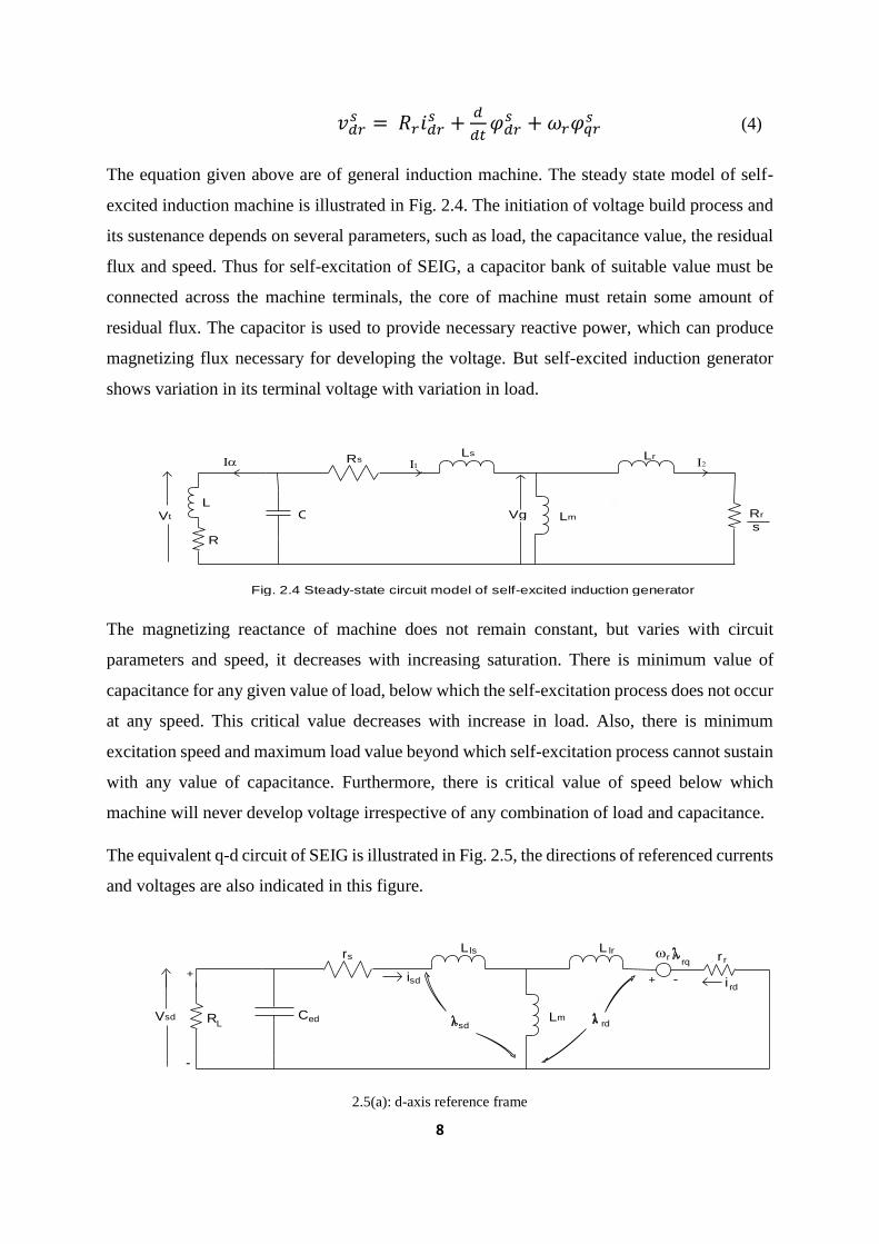
The equation given above are of general induction machine. The steady state model of self-
excited induction machine is illustrated in Fig. 2.4. The initiation of voltage build process and
its sustenance depends on several parameters, such as load, the capacitance value, the residual
flux and speed. Thus for self-excitation of SEIG, a capacitor bank of suitable value must be
connected across the machine terminals, the core of machine must retain some amount of
residual flux. The capacitor is used to provide necessary reactive power, which can produce
magnetizing flux necessary for developing the voltage. But self-excited induction generator
shows variation in its terminal voltage with variation in load.
The magnetizing reactance of machine does not remain constant, but varies with circuit
parameters and speed, it decreases with increasing saturation. There is minimum value of
capacitance for any given value of load, below which the self-excitation process does not occur
at any speed. This critical value decreases with increase in load. Also, there is minimum
excitation speed and maximum load value beyond which self-excitation process cannot sustain
with any value of capacitance. Furthermore, there is critical value of speed below which
machine will never develop voltage irrespective of any combination of load and capacitance.
The equivalent q-d circuit of SEIG is illustrated in Fig. 2.5, the directions of referenced currents
and voltages are also indicated in this figure.
2.5(a): d-axis reference frame
Vt
L
R
C Lm
Lr
Rr
s
LsRs
Vg
Fig. 2.4 Steady-state circuit model of self-excited induction generator
Vsd R C Lm
Lr
L rrq r r
lrlss
edL
i rdisd + -
sd rd
+
-
Page 21
9
2.5(b): q-axis reference frame
Fig. 2.5 Dynamic d-q model of SEIG in Stationary reference frame
Applying KVL in q-d model of SEIG, we get following equations
𝑉𝑠𝑑 = (𝑟𝑠 + 𝑝𝐿𝑙𝑠)𝑖𝑠𝑑 + 𝑝𝐿𝑚(𝑖𝑠𝑑 + 𝑖𝑟𝑑) (5)
𝑉𝑠𝑞 = (𝑟𝑠 + 𝑝𝐿𝑙𝑠)𝑖𝑠𝑞 + 𝑝𝐿𝑚(𝑖𝑠𝑞 + 𝑖𝑟𝑞) (6)
𝑖𝑟𝑑𝑟𝑟 + 𝜔𝑟𝜆𝑟𝑞 + 𝑝(𝐿𝑚 + 𝐿𝑙𝑟)𝑖𝑟𝑑 + 𝑝𝐿𝑚𝑖𝑠𝑑 = 0 (7)
𝑖𝑟𝑞𝑟𝑟 − 𝜔𝑟𝜆𝑟𝑑 + 𝑝(𝐿𝑚 + 𝐿𝑙𝑟)𝑖𝑟𝑞 + 𝑝𝐿𝑚𝑖𝑠𝑞 = 0 (8)
Where, 𝜆𝑟𝑑 = 𝐿𝑟𝑖𝑟𝑑 + 𝐿𝑚𝑖𝑠𝑑 , 𝜆𝑟𝑞 = 𝐿𝑟𝑖𝑟𝑞 + 𝐿𝑚𝑖𝑠𝑞
𝐿𝑟 = 𝐿𝑙𝑟 + 𝐿𝑚 , 𝐿𝑠 = 𝐿𝑙𝑠 + 𝐿𝑚
Using q-d components of stator current (𝑖𝑠𝑑 and 𝑖𝑠𝑞 ) and rotor current (𝑖𝑟𝑑 and 𝑖𝑟𝑞) as state
variables, the following differential equations 9-12 are derived
𝑑𝑖𝑠𝑑
𝑑𝑡=
1
𝐿𝑟𝐿𝑠−𝐿𝑚2 [𝐿𝑟𝑣𝑠𝑑 − 𝐿𝑟𝑟𝑠𝑖𝑠𝑑 + 𝐿𝑚𝑟𝑟𝑖𝑟𝑑 + 𝐿𝑚𝜔𝑟𝐿𝑟𝑖𝑟𝑞 + 𝜔𝑟𝐿𝑚
2 𝑖𝑠𝑞] (9)
𝑑𝑖𝑠𝑞
𝑑𝑡=
1
𝐿𝑟𝐿𝑠−𝐿𝑚2 [𝐿𝑟𝑣𝑠𝑞 − 𝐿𝑟𝑟𝑠𝑖𝑠𝑞 + 𝐿𝑚𝑟𝑟𝑖𝑟𝑞 − 𝐿𝑚𝜔𝑟𝐿𝑟𝑖𝑟𝑑 − 𝜔𝑟𝐿𝑚
2 𝑖𝑠𝑑] (10)
𝑑𝑖𝑟𝑑
𝑑𝑡=
1
𝐿𝑟𝐿𝑠−𝐿𝑚2 [−𝐿𝑚𝑣𝑠𝑑 − 𝑟𝑟𝐿𝑠𝑖𝑟𝑑 − 𝜔𝑟𝐿𝑠𝐿𝑟𝑖𝑟𝑞 − 𝜔𝑟𝐿𝑚𝐿𝑠𝑖𝑠𝑞 + 𝐿,𝑚𝑟𝑠𝑖𝑠𝑑] (11)
𝑑𝑖𝑟𝑞
𝑑𝑡=
1
𝐿𝑟𝐿𝑠−𝐿𝑚2 [−𝐿𝑚𝑣𝑠𝑞 − 𝑟𝑟𝐿𝑠𝑖𝑟𝑞 + 𝜔𝑟𝐿𝑠𝐿𝑟𝑖𝑟𝑑 + 𝜔𝑟𝐿𝑚𝐿𝑠𝑖𝑠𝑑 + 𝐿,𝑚𝑟𝑠𝑖𝑠𝑞] (12)
Vsq R C Lm
Lr
L rrd r r
lrlss
eqL
i rqisq + -
sq rq
+
-
Page 22
10
The electromagnetic torque can be calculated as follows
𝑇𝑒 = (3
2) (
𝑃
2) 𝐿𝑚[𝑖𝑠𝑞𝑖𝑟𝑑 − 𝑖𝑠𝑑𝑖𝑟𝑞] (13)
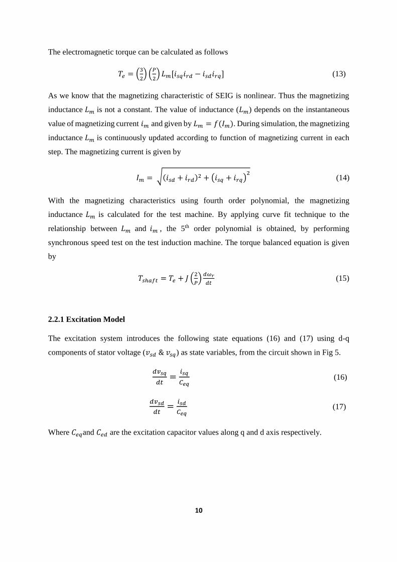
As we know that the magnetizing characteristic of SEIG is nonlinear. Thus the magnetizing
inductance 𝐿𝑚 is not a constant. The value of inductance (𝐿𝑚) depends on the instantaneous
value of magnetizing current 𝑖𝑚 and given by 𝐿𝑚 = 𝑓(𝐼𝑚). During simulation, the magnetizing
inductance 𝐿𝑚 is continuously updated according to function of magnetizing current in each
step. The magnetizing current is given by
𝐼𝑚 = √(𝑖𝑠𝑑 + 𝑖𝑟𝑑)2 + (𝑖𝑠𝑞 + 𝑖𝑟𝑞)2 (14)
With the magnetizing characteristics using fourth order polynomial, the magnetizing
inductance 𝐿𝑚 is calculated for the test machine. By applying curve fit technique to the
relationship between 𝐿𝑚 and 𝑖𝑚 , the 5th order polynomial is obtained, by performing
synchronous speed test on the test induction machine. The torque balanced equation is given
by
𝑇𝑠ℎ𝑎𝑓𝑡 = 𝑇𝑒 + 𝐽 (2
𝑃)
𝑑𝜔𝑟
𝑑𝑡 (15)
2.2.1 Excitation Model
The excitation system introduces the following state equations (16) and (17) using d-q
components of stator voltage (𝑣𝑠𝑑 & 𝑣𝑠𝑞) as state variables, from the circuit shown in Fig 5.
𝑑𝑣𝑠𝑞
𝑑𝑡=
𝑖𝑠𝑞
𝐶𝑒𝑞 (16)
𝑑𝑣𝑠𝑑
𝑑𝑡=
𝑖𝑠𝑑
𝐶𝑒𝑞 (17)
Where 𝐶𝑒𝑞and 𝐶𝑒𝑑 are the excitation capacitor values along q and d axis respectively.
Page 23
11
2.2.2 Load Modelling
The d and q axis current equations for the resistive balanced is given by following equations
𝑖𝑅𝑞 =𝑣𝑠𝑞
𝑅𝐿 (18)
𝑖𝑅𝑑 =𝑣𝑠𝑑
𝑅𝐿 (19)
The d and q axes current equations for the balanced R-L load are derived from Fig. 5, and given
by equations 20 and 210
𝑖𝑅𝑞 =(𝑣𝑠𝑞−𝑅𝐿𝑖𝑅𝑞)
𝑝𝐿𝐿 (20)
𝑖𝑅𝑑 =(𝑣𝑠𝑑−𝑅𝐿𝑖𝑅𝑑)
𝑝𝐿𝐿 (21)
If the load is capacitive in nature, then the capacitor value will be added to the excitation
capacitor value.
2.3 Voltage build-up process in SEIG
The induction machine can be operate in standalone mode, if excited by suitable value of
capacitor. When static capacitor are connected in shunt across the stator terminals of induction
machine, voltage will be induced at its terminals provided the machine is driven by prime
mover. For successful excitation machine must sustain small value of residual flux. This
residual flux in the core of machine induces a small alternating voltage in the stator, this voltage
induced is applied to the capacitor which generates a lagging magnetizing current which flows
in stator windings. If the capacitance is of proper value, the current that flow in stator winding
will be large enough to further increase the flux value already existing in air gap. With increase
of air gap flux, the stator terminal voltage further increase which result in increase in
magnetizing current drawn by capacitor and hence air gap flux further increases. This process
goes on until the terminal voltage of generator reaches its rated value. The steady state value
of terminal voltage is determine by the capacitive reactance of the connected capacitance and
the saturation curve of the machine. Fig. 2.6. Represents the voltage developed Vt as a function
of Im, which determine the steady state point of voltage build up.
Page 24
12
2.4 Simulation of SEIG driven by constant speed prime mover in MATLAB/SIMULINK
The SEIG’s dynamic model is developed using equations (5)-(19) in MATLAB/SIMULINK
environment. The process of self-excitation is based on residual magnetism present in the rotor
circuit and voltage build is excited by reactive power supplied by the capacitor. After the
voltage is reaches to a steady state value, load is connected to the SEIG. The specification of
induction machine is taken from [29] and is given below.
Induction machine rating: - 3.7kW, 415V, 7.5A, 4-Pole and its parameters are as follows:
𝑟𝑠(Ω) 𝑟𝑟(Ω) 𝑋𝑙𝑠(Ω) 𝑋𝑙𝑠(Ω) 𝐿𝑚(H) 𝐽 (𝐾𝑔 𝑚2)
7.34 5.64 6.7 6.7 0.5 0.16
The magnetizing characteristic equation and constants are:
𝐿𝑚 = 𝑏0 + 𝑏𝐼𝑚 + 𝑏2𝐼𝑚2 + 𝑏𝐼𝑚
3 + 𝑏4𝐼𝑚4 + 𝑏5𝐼𝑚
5
Where 𝑏0 = 1.043, 𝑏1 = -0.853, 𝑏2 = 0.713, 𝑏3 = -0.304, 𝑏4 = 0.0576, 𝑏5 = -0.0038
The performance characteristics of SEIG under the following condition has been observed.
1. Voltage build-up process
2. Switching in of load
3. Loss of excitation due to heavy-load
Vt
m Xc
Voltage (V)
Magnetizing current m (A)
Fig. 2.6 Determination of Stable Operation of SEIG
Page 25
13
The three phase voltages and currents are obtained by applying d-q to a-b-c transformation as
follows:
[
𝑤𝑎
𝑤𝑏
𝑤𝑐
] =
[ 1 0
−1
2−
√3
2
−1
2
√3
2 ]
[𝑤𝑠𝑞
𝑤𝑠𝑑] (22)
Where, 𝑤𝑎 , 𝑤𝑏 𝑎𝑛𝑑 𝑤𝑐are three phase voltage or current quantities and 𝑤𝑠𝑞 and 𝑤𝑠𝑑 are two
phase voltage or current quantities. The value of peak voltage is calculated as:
𝑉𝑚 = √2
3(𝑣𝑎𝑛
2 + 𝑣𝑏𝑛2 + 𝑣𝑐𝑛
2 ) (23)
𝑣𝑎𝑛 = 𝑉𝑚 sin(𝜔𝑡), 𝑣𝑏𝑛 = 𝑉𝑚 sin (𝜔𝑡 −2𝛱
3), 𝑣𝑐𝑛 = 𝑉𝑚 sin (𝜔𝑡 +
2𝛱
3)
A 61.6 µF capacitor is used for excitation in generator. The SEIG is driven at synchronous
speed of speed of 157.07 rad/s. The developed SEIG model is simulated in MATALB by using
the numerical integration technique Runge-kutta fourth order method. The step length should
be as small as possible for getting accurate and precise result, here it is taken between 1𝑒−6
to 5𝑒−6. In case of the SEIG the dynamics of voltage build up and stabilization mainly depends
on the variation of magnetization inductance of machine. From the synchronous speed test, the
magnetizing inductance 𝐿𝑚 is obtained as function of magnetizing current 𝐼𝑚 . The initial
values of input states of q-d model i.e.𝑖𝑠𝑑, 𝑖𝑠𝑞, 𝑖𝑟𝑑, 𝑖𝑟𝑞 are assumed to be zero. For the self-
excitation the residual magnetism of the machine is taken as initial values of 𝑣𝑠𝑞 and 𝑣𝑠𝑑. The
Simulink model of SEIG is shown in Fig. 2.7(a). Fig. 2.7(b) shows the subsystem of d-q
induction generator model. Fig. 2.7(c) shows the system of stator and rotor d-q axis current
derivation equations. Fig. 2.7(d) show the subsystem of dq-abc conversion and Fig. 2.7(e)
shows the excitation capacitance sub-system.
Page 26
14
Fig. 2.7(a) Simulink model of SEIG in MATLAB
Fig. 2.7(b) Subsystem of d-q Induction generator model
Fig. 2.7(c) subsystem of stator and rotor d-q axis current derivation
Page 27
15
Fig. 2.7(d) d-q to abc conversion Fig. 2.7(e) Subsystem of excitation capacitor
2.5 Results and Discussion
2.5.1 Self-excitation process
The generator is driven at synchronous speed of 157.07 rad/s and a three phase delta connected
capacitor is bank of 61.6µF is switched in to its terminals. The residual magnetism taken in
terms of 𝑣𝑠𝑞 and𝑣𝑠𝑑 as 1 volt, which induces the voltage across self-exciting capacitors and
thus producing magnetizing current in the stator resulting in higher voltage. This process goes
on until the magnetic field reaches to its saturation. The simulation results of self-excitation
process are shown in Fig. 2.8 (a)-(d). Fig. 2.8(a) shows the peak phase voltage of SEIG
terminal, the SEIG steady state voltage peak voltage is 335 V (236 V RMS), which reaches
steady state in 0.35 sec. Fig. 2.8 (b) shows the phase voltage of SEIG terminals. The steady
state value of stator current at no load is 6.5 A and is shown in Fig. 2.8 (c) for phase a. Fig. 2.8
(d) shows the magnetizing current waveform and it attains its steady state value of 2.656 A at
3.5 sec.
Fig. 2.8(a) Peak SEIG terminal voltage waveform
0 0.2 0.4 0.6 0.8 10
100
200
300
400
Time (sec)
Vm
(V)
Page 28
16
Fig. 2.8 (b) Phase ‘a’ current of SEIG at no load
Fig. 2.8 (c) Waveform of SEIG terminal voltage (phase voltage)
Fig. 2.8 (d) Magnetizing current waveform
2.5.2 Insertion of Load
Initially the SEIG is running at no load and steady state voltage and current are developed.
Now at time t = 0.8 sec a balanced R-L load of 1 KW at 0.8 pf is suddenly connected to the
SEIG terminals. It is observed that the steady state peak voltage at no load is 337 V, which
reduces to 278 V when load is connected, as illustrated in Fig 2.9(a). Fig. 2.9(b) illustrates the
phase voltage of SEIG with insertion of load. When generator is operating at no load, the load
current is zero, but with load connection the current reaches a peak value of 1.1A and shown
in Fig. 2.9(c). The stator current at steady state at no load is 6.5A, but it reduces to 4.75A when
load is connected, shown in Fig. 2.9(d). With application of load the magnetizing current Im
decreases Fig. 2.9(e), which results in the reduced flux. With reduction in flux, the value of
induced voltage also decreases.
0 0.2 0.4 0.6 0.8 1
-8
-4
0
4
8
Time (sec)
Is (A
)
0 0.2 0.4 0.6 0.8 1-400
-200
0
200
400
Time (sec)
Vabc (
V)
0 0.2 0.4 0.6 0.8 10
1
2
3
Time (sec)
Im (
A)
Page 29
17
Fig. 2.9(a) SEIG peak voltage Waveform
Fig. 2.9(b) Stator terminal phase voltage waveform
Fig. 2.9(c) Load current waveform
Fig. 2.9(d) Stator current Waveform
Fig. 2.9(e) Magnetizing current waveform
0 0.4 0.8 1.2 1.50
100
200
300350
Time (sec)
Vm
(V
)
0 0.4 0.8 1.2 1.5-400
-200
0
200
400
Time (sec)
Vab
c (V
)
0 0.4 0.8 1.2 1.5-2
-1
0
1
2
Time (sec)
Load
Cul
lent
(A
)
0 0.4 0.8 1.2 1.5
-8
-4
0
4
8
Time (sec)
Is (
A)
0 0.4 0.8 1.2 1.50
1
2
3
Time (sec)
Im (
A)
Page 30
18
2.5.3 Loss of Excitation due to heavy-load
The SEIG which is initially operated under steady state condition having peak value of voltage
335 volts and R-L load of 0.5 KW is applied at t=0.8seonds having pf 0.8, voltage is reduced
and reached a steady state voltage of 278 volt. At t=1.3 seconds an extra load is applied, of
value 2.5KW R-L load, the SEIG line voltage collapse is a monotonous decay of the voltage
nearly to zero shown in Fig. 2.10(a). Once the voltage collapse occurs, the re-excitation of the
generator becomes difficult. Thus it shows the poor overloading capability of the SEIG.
Therefore the load connected to the generator should never exceed beyond the maximum load
the generator can deliver under steady state condition. But it may be mentioned here that the
momentary excess stator current can operate protective relays to isolate the overload condition
at the generator terminals to prevent voltage collapse. Fig. 2.10(b) shows the terminal voltage
of SEIG. With increase in load, beyond its maximum value, the magnetizing current falls to
zero as shown in Fig. 2.10(c).
Fig. 2.10(a) SEIG peak voltage waveform
Fig. 2.10(b) SEIG terminal voltage (phase)
Fig. 2.10(c) Magnetizing current waveform
0 0.4 0.8 1.2 1.6 1.80
100
200
300
400
Time (sec)
Vm
0 0.4 0.8 1.2 1.6 1.8-400
-200
0
200
400
Time (sec)
Vab
c (
V)
0 0.4 0.8 1.2 1.6 1.80
1
2
3
Time (sec)
Im
Page 31
19
2.5.4 Step change in prime mover speed
When rotor speed changes from 157 rad/s to 165 rad/s at 0.6 sec by prime mover, the
mechanical input from prime mover increases and this causes the increase in stator terminal
voltage as illustrated in Fig. 2.11(a). The peak steady-state voltage increases from 335 V to 365
V. Fig. 2.11(b) shows the magnetizing voltage waveform, which increase from 2.6 A to 3 A.
Fig. 2.11(a) SEIG peak voltage waveform
Fig. 2.11(b) Magnetizing current waveform
Fig. 2.12 illustrates the steady-state waveform of SEIG terminal voltage with peak value of 335
V and SEIG line for phase ‘a’ with peak value of 6.8 A
Fig. 2.12 Steady state waveform during voltage build-up
0 0.2 0.4 0.6 0.8 10
100
200
300
400
Time (sec)
Vm
(V
)
0 0.2 0.4 0.6 0.8 10
1
2
3
4
Time (sec)
Im (
A)
0.4 0.41 0.42 0.43 0.44 0.45-400
-200
0
200
400
Time (sec)
Vab
c (V
)
0.4 0.41 0.42 0.43 0.44 0.45-10
-5
0
5
10
Time (sec)
Isa
(A)
Page 32
20
2.6 Conclusion
The self-excitation process of SEIG depends on load, capacitance value and speed of rotor. For
maintaining the voltage of SEIG constant at its rated value a controller is required. The
standalone system controller should be such that it is simple, reliable, low cost, easy to
implement and has faster response. Thus, controller is required to develop by taking non-linear
and linear load.
Page 33
21
Chapter-3
MODELLING OF STATCOM BASED VOLTAGE
CONTROLLER FOR SEIG DRIVEN BY CONSTANT SPEED
PRIME MOVER USING CONVENTIONAL PI CONTROLLER
3.1 Introduction
In chapter 2, we have seen that will sudden application of load or change in rotor speed causes
the variation in SEIG terminal voltage. For regulating voltage various controllers are developed
by researchers [15]-[28]. Earlier attempts were made for regulating the voltage of SEIG by
using thyristor controlled inductor and fixed capacitor [20], and short-shunt connections of
capacitor [21]. But the voltage control provided by this type of controllers are discrete in nature
and produces harmonics in the voltage waveform. With the advent of solid state devices, the
control of SEIG terminal voltage has become more effective and reliable, as it can provide
variable reactive power to generator and load to keep the terminal voltage constant with varying
load conditions. Geng e.al. [23] Proposed the direct voltage control (DVC) strategy using PI
regulator with a feed-forward compensator and lead-lag corrector. But its implementation is
very complex because of design of lead-lag corrector and complexity involve in feed-forward
compensator. Singh et al. [38] has proposed a static synchronous series compensator (SSSC)
and static compensator (STATCOM) to feed static and dynamic load. These controllers are not
designed for non-linear loads, also the dynamic response of controller is very poor.
This chapter present the analysis and development of STATCOM based voltage regulator for
SEIG using conventional PI Controller feeding balanced or unbalanced load or linear and non-
linear loads. The STATCOM eliminates the harmonics present in the system, it also provide
load balancing and reactive power fulfilment as demanded by load and generator.
3.2 About STATCOM
The STATCOM consist of three phase current controlled voltage source inverter (CC-VSI)
with IGBTS used as switches, a dc bus capacitor, ac inductors (for removing harmonics) and
two conventional PI controller. The excitation capacitors in SEIG are used to generate the rated
voltage of SEIG at no load. When load is applied, the additional demand of reactive power of
Page 34
22
load is fulfilled by STATCOM. The STATCOM acts as source of leading or lagging power
supply depending on loading conditions. The dc bus capacitor act as energy storage device and
provide reactive power as demanded by load. The block diagram of STATCOM with SEIG 7is
shown in Fig. 2.1 along with control scheme applied to STATCOM for generating the gate
signals.
Fig. 3.1(a)
S1
b
S
S S
S S 2
3
4
5
6
Cdc
Vdc
Lf
i la
i
i
ma
lc
i
i
i
sa
sb
sc
a
b
c
a
bc
Prime
Movera
c
i a
i b
i c
icc
icaicb
Cc Ca
Cb
igc iga
igb
STATCOM
+
-
Vab
Vbc
Vca
mb
mc
i
i
Linear/
Non-
Linear
Load
ilb
Page 35
23
3.1(b)
Fig. 3.1 (a) Schematic diagram of SEIG-STATCOM system, (b) Control scheme applied to
SEIG-STATCOM
3.2.1 Control scheme for SEIG
For controlling the voltage of SEIG, the source current is controlled which composed of two
component in phase component and quadrature component. For maintaining the terminal
voltage constant of SEIG, two control loops are deployed in STATCOM for generating
reference supply current. The in-phase unit vectors are three phase sinusoidal functions of unit
Unit Voltagetemplate generator
Va Vb Vc
uaubuc
In-phase
component
refrence current
DC Voltage
P I
Controller
Quadrature Voltagetemplate generatorw wb wc
au u ub c
AC Voltage
P I
Controller
Quadrature
Component
Reference Current
a
++
isaq*
isbq*
iscq*
isad* isbd
*iscd*
i sa*
PWM Current
Controller
i sb* i sc
*i sa
ismq*
i sb
i sc
S1
b
S
S S
S S 2
3
4
5
6
Cdc
Vdc
L f
ac
STATCOM
+
-
mb
mc
Vdc
Vdcref+
-
i smd*
i
i
imaa
b
c
S1 to S6
Vpref
Vp
+-
Page 36
24
amplitude (𝑢𝑎 , 𝑢𝑏 , 𝑢𝑐). These are computed by diving three phase ac voltage( 𝑣𝑎,𝑣𝑏 , 𝑣𝑐) by
their amplitude 𝑉𝑝. The quadrature unit vectors are also three phase unit sinusoidal functions
(𝑤𝑎, 𝑤𝑏 , 𝑤𝑐) , which are computed from in-phase vectors. There are two conventional PI
controllers employed for maintaining the SEIG voltage constant. One PI controller sensed the
input error, computed from the difference of reference ac voltage (𝑉𝑝𝑟𝑒𝑓) with amplitude of ac
voltage (𝑉𝑝). The output of obtained from this ac PI controller is taken as reference peak value
of quadrature supply current component (𝑖𝑠𝑚𝑞∗ ), this current (𝑖𝑠𝑚𝑞
∗ ) decided the amplitude of
reactive current which is generated by the STATCOM. The quadrature unit vectors
(𝑤𝑎, 𝑤𝑏 , 𝑤𝑐) are multiplied with the output of ac voltage PI controller (𝑖𝑠𝑚𝑞∗ ) which generates
the quadrature component (𝑖𝑠𝑎𝑞∗ , 𝑖𝑠𝑏𝑞
∗ , 𝑖𝑠𝑐𝑞∗ ). of the reference supply current. The STATCOM
uses capacitor as a dc bus which provided necessary reactive power requirement to the SEIG.
The value of capacitor voltage (𝑉𝑑𝑐) is sensed and fed to comparator along with the dc reference
voltage (𝑉𝑑𝑐𝑟𝑒𝑓). The error is given to another conventional PI controller known as dc PI
controller. The output of this PI controller yields reference peak in-phase supply current
component ( 𝑖𝑠𝑚𝑞∗ ). This component ( 𝑖𝑠𝑚𝑞
∗ ) decides the amplitude of the active power
component of source current. The in-phase component (𝑖𝑠𝑎𝑑∗ , 𝑖𝑠𝑏𝑑
∗ , 𝑖𝑠𝑐𝑑∗ ) of reference supply
current are generated by the multiplication of in-phase (𝑢𝑎 , 𝑢𝑏 , 𝑢𝑐) unit vectors with the output
of dc PI controller. The sum of quadrature (𝑖𝑠𝑎𝑞∗ , 𝑖𝑠𝑏𝑞
∗ , 𝑖𝑠𝑐𝑞∗ ) reference current and in-phase
(𝑖𝑠𝑎𝑑∗ , 𝑖𝑠𝑏𝑑
∗ , 𝑖𝑠𝑐𝑑∗ ) reference current gives the reference source current (𝑖𝑠𝑎
∗ , 𝑖𝑠𝑏∗ , 𝑖𝑠𝑐
∗ ). The reference
source currents then compared with the sensed source line currents (𝑖𝑠𝑎, 𝑖𝑠𝑏 , 𝑎𝑛𝑑 𝑖𝑠𝑐) and the
error is given to pulse width modulation (PWM) current controller to generate switching signals
for IGBTs used in VSI.
Non-linear loads draw non-sinusoidal currents which composed of both fundamental as well
as harmonics components of current. This non-sinusoidal current causes to inject harmonics in
the systems and resulting in distortion of terminal voltage. Unbalanced loads draws unbalanced
currents (composed of negative and positive sequence components) due to which the machine
has to be used under derated condition. But the STATCOM filter out the harmonics and
balances the unbalanced load, resulting in sinusoidal voltage and current of SEIG and also
regulating its terminal voltage.
Page 37
25
3.3 Modelling of SEIG-STATCOM
The SEIG-STATCOM system consist of SEIG, STATCOM, and the control technique involve
and load. The dynamic model of each system components are discussed below.
3.3.1 Modelling of control scheme involved
The components of SEIG-STATCOM system are given in Fig. 3.1(a) and its control scheme
applied to SEIG is illustrated in Fig. 3.1(b), which are modelled as follows
The SEIG terminal ( 𝑣𝑎, 𝑣𝑏, 𝑣𝑐) phase voltages are sensed, which are sinusoidal in nature and
their peak value is computed as follows
𝑉𝑝 = √(2
3) (𝑣𝑎
2 + 𝑣𝑏2 + 𝑣𝑐
2) (24)
The in-phase unit vectors are computed as
𝑢𝑎 =𝑣𝑎
𝑉𝑡 , 𝑢𝑏 =
𝑣𝑏
𝑉𝑡 , 𝑢𝑏 =
𝑣𝑏
𝑉𝑡 (25)
The unit vectors in quadrature are derived from unit in-phase vectors as follows
[
𝑤𝑎
𝑤𝑏
𝑤𝑐
] =
[ 0
−1
√3
1
√3
√3
2
1
2√3
−1
2√3
−√3
2
1
2√3
−1
2√3]
[
𝑢𝑎
𝑢𝑏
𝑢𝑐
] (26)
1) Quadrature Component of Reference Source Currents:
The voltage error computed at 𝑛th sampling instant is
𝑉𝑒(𝑛) = 𝑉𝑝𝑟𝑒𝑓 − 𝑉𝑝(𝑛) (27)
Where, 𝑉𝑝𝑟𝑒𝑓 is peak of reference terminal voltage of SEIG and 𝑉𝑝(𝑛) is the amplitude
of sensed SEIG terminal voltage at 𝑛 th sampling. The output of ac PI controller
(𝑖𝑠𝑚𝑞∗ (𝑛)) for regulating the SEIG terminal voltage at 𝑛th sampling instant is expressed
as
𝑖𝑠𝑚𝑞∗ (𝑛) = 𝑖𝑠𝑚𝑞
∗ (𝑛 − 1) + 𝐾𝑝𝑎𝑐{𝑉𝑒𝑟(𝑛) − 𝑉𝑒(𝑛 − 1)} + 𝐾𝑖𝑎𝑐𝑉𝑒(𝑛) (28)
Page 38
26
Where, 𝐾𝑝𝑎𝑐 and 𝐾𝑖𝑎𝑐 are proportional and integral gain constant of ac PI controller,
𝑉𝑒(𝑛) and 𝑉𝑒(𝑛 − 1) are voltage errors at 𝑛 th and (𝑛 -1)th sampling instant
respectively.
The 𝑖𝑠𝑚𝑞∗ (𝑛) is the amplitude of quadrature component of reference current computed
at 𝑛th instant. Thus quadrature components of reference source currents are calculated
as
𝑖𝑠𝑎𝑞∗ = 𝑖𝑠𝑚𝑞
∗ 𝑤𝑎; 𝑖𝑠𝑏𝑞∗ = 𝑖𝑠𝑚𝑞
∗ 𝑤𝑏; 𝑖𝑠𝑐𝑞∗ = 𝑖𝑠𝑚𝑞
∗ 𝑤𝑐 (29)
2) In-phase Component of Reference Source Currents:
The dc bus capacitor voltage error computed at 𝑛th sampling instant is expressed as
𝑉𝑑𝑐𝑒(𝑛) = 𝑉𝑑𝑐𝑟𝑒𝑓 − 𝑉𝑑𝑐(𝑛) (30)
Where, 𝑉𝑑𝑐𝑟𝑒𝑓 is reference dc bus voltage, 𝑉𝑑𝑐(𝑛) is the sensed dc bus voltage at 𝑛th
sampling and 𝑉𝑑𝑐𝑒(𝑛) is the voltage error at 𝑛th sampling instant. The output of dc PI
controller at 𝑛th instant is expressed as
𝑖𝑠𝑚𝑑∗ (𝑛) = 𝑖𝑠𝑚𝑑
∗ (𝑛 − 1) + 𝐾𝑝𝑑𝑐{𝑉𝑑𝑐𝑒(𝑛) − 𝑉𝑑𝑐𝑒(𝑛 − 1)} + 𝐾𝑖𝑑𝑉𝑑𝑐𝑒(𝑛) (31)
Where, 𝐾𝑝𝑑𝑐 and 𝐾𝑖𝑑𝑐 are proportional and integral gain constant of PI controller of dc
bus. The 𝑖𝑠𝑚𝑑∗ (𝑛) is the amplitude of active power component of source current. The
in-phase components of reference source current are calculated as
𝑖𝑠𝑎𝑑∗ = 𝑖𝑠𝑚𝑑
∗ 𝑢𝑎; 𝑖𝑠𝑏𝑑∗ = 𝑖𝑠𝑚𝑑
∗ 𝑢𝑏; 𝑖𝑠𝑐𝑑∗ = 𝑖𝑠𝑚𝑑
∗ 𝑢𝑐 (32)
3) Evaluation of total source reference currents:
For generating source reference currents, the in-phase reference current components
and quadrature components of reference current are added together to generate the
source reference current as follows
𝑖𝑠𝑎∗ = 𝑖𝑠𝑎𝑞
∗ + 𝑖𝑠𝑎𝑑∗
𝑖𝑠𝑏∗ = 𝑖𝑠𝑏𝑞
∗ + 𝑖𝑠𝑏𝑑∗ (33)
Page 39
27
𝑖𝑠𝑐∗ = 𝑖𝑠𝑐𝑞
∗ + 𝑖𝑠𝑐𝑑∗
4) PWM Current Controller:
The source reference current (𝑖𝑠𝑎∗ , 𝑖𝑠𝑏
∗ , 𝑖𝑠𝑐∗ ) and sensed source current (𝑖𝑠𝑎, 𝑖𝑠𝑏 , 𝑖𝑠𝑐) are
fed to comparator and error produced is amplified and given to PWM current controller.
The PWM controller generates the switching pulses (ON/OFF) of the IGBTs of VSI.
The current errors are calculated as
𝑖𝑠𝑎𝑒𝑟 = 𝑖𝑠𝑎∗ − 𝑖𝑠𝑎; 𝑖𝑠𝑏𝑒𝑟 = 𝑖𝑠𝑏
∗ − 𝑖𝑠𝑏; 𝑖𝑠𝑐𝑒𝑟 = 𝑖𝑠𝑐∗ − 𝑖𝑠𝑐 (34)
These current error signals and a triangular carrier wave signal are fed to comparator to
generate switching pulses for IGBTs. Corresponding to phase a ( 𝑖𝑠𝑎𝑒𝑟) if current error
is greater in magnitude than the triangular carrier wave, the switch 𝑆1 (upper device) of
phase ‘a’ leg of VSI is turned ON and switch 𝑆4 (lower device) of phase ‘a’ of VSI is
turned OFF, and value of switching function 𝐹𝐴 is set to zero. If the current error is
less in magnitude than the triangular carrier wave signal, then switch 𝑆1 of VSI is turned
OFF and switch 𝑆4 is turned ON, and the value of 𝐹𝐴 is set to one. For other switches
same logic same logic is applied for phase ‘b’ (𝑆3 & 𝑆6) and phase ‘c’ (𝑆5 & 𝑆2).
3.3.2 Modelling of STATCOM
The modelling of STATCOM is done as follows. The STATCOM bus voltage in derivative
form is represent as
𝑝𝑣𝑑𝑐 = (𝑖𝑐𝑎𝐹𝐴 + 𝑖𝑐𝑏𝐹𝐵 + 𝑖𝑐𝑐𝐹𝐶)/𝐶𝑑𝑐 (35)
Where, 𝑆𝐴, 𝑆𝐵 and 𝑆𝐶 are switching functions for ON/OFF positions of Voltage Source
Inverter (VSI) switches 𝑆1 − 𝑆6.
The three phase ac line voltage of PWM conveter (𝑓𝑎, 𝑓𝑏 , 𝑓𝑐) which reflects from the dc bus
voltage are expressed as
𝑓𝑎 = 𝑣𝑑𝑐(𝐹𝐴 − 𝐹𝐵)
𝑓𝑏 = 𝑣𝑑𝑐(𝐹𝐵 − 𝐹𝐶)
Page 40
28
𝑓𝑐 = 𝑣𝑑𝑐(𝐹𝐶 − 𝐹𝐴) (36)
The voltage and current equations for the output of VSI of STATCOM are expressed as follows
𝑣𝑎 = 𝑅𝑓𝑖𝑐𝑎 + 𝐿𝑓𝑝𝑖𝑐𝑎 + 𝑓 − 𝑅𝑓𝑖𝑐𝑏 − 𝐿𝑓𝑝𝑖𝑐𝑏 (37)
𝑣𝑏 = 𝑅𝑓𝑖𝑐𝑏 + 𝐿𝑓𝑝𝑖𝑐𝑏 + 𝑓𝑏 − 𝑅𝑓𝑖𝑐𝑐 − 𝐿𝑓𝑝𝑖𝑐𝑐 (38)
𝑖𝑐𝑎 + 𝑖𝑐𝑏 + 𝑖𝑐𝑐 = 0 (39)
The value of 𝑖𝑐𝑐 obtained from equation (39) is substituted into equation (38) which gives
𝑣𝑏 = 𝑅𝑓𝑖𝑐𝑏 + 𝐿𝑓𝑝𝑖𝑐𝑏 + 𝑓𝑏 + 𝑅𝑓𝑖𝑐𝑎 + 𝐿𝑓𝑝𝑖𝑐𝑎 + 𝑅𝑓𝑖𝑐𝑏 + 𝐿𝑓𝑝𝑖𝑐𝑏 (40)
By rearranging equations (37) and (40), we get
𝐿𝑓𝑝𝑖𝑐𝑎 − 𝐿𝑓𝑝𝑖𝑐𝑏 = 𝑣𝑎 − 𝑓𝑎 − 𝑅𝑓𝑖𝑐𝑎 + 𝑅𝑓𝑖𝑐𝑏 (41)
𝐿𝑓𝑝𝑖𝑐𝑎 + 2𝐿𝑓𝑝𝑖𝑐𝑏 = 𝑣𝑏 − 𝑓𝑏 − 𝑅𝑓𝑖𝑐𝑎 − 2𝑅𝑓𝑖𝑐𝑏 (43)
Hence, the STATCOM equations are obtained by solving (41) and (42)
𝑝𝑖𝑐𝑎 = {(𝑣𝑏 − 𝑓𝑏) + 2(𝑣𝑎 − 𝑓𝑎) − 3𝑅𝑓𝑖𝑐𝑎}/(3𝐿𝑓) (44)
𝑝𝑖𝑐𝑏 = {(𝑣𝑏 − 𝑓𝑏) − (𝑣𝑎 − 𝑓𝑎) − 3𝑅𝑓𝑖𝑐𝑎}/(3𝐿𝑓) (45)
3.3.3 Modelling of SEIG
The dynamic modelling of SEIG is already presented in chapter-2. Here it is again discussed
in brief. The dynamic model is developed using stationary d-q reference frames, whose voltage
equations are
[𝑣] = [𝑟][𝑖] + [𝐿]𝑝[𝑖] + 𝑊𝑔[𝐺][𝑖] (46)
The current equation is derived from (46) and expressed as
𝑝[𝑖] = [𝐿]−1([𝑣] − [𝑟][𝑖] − 𝑊𝑔[𝐺][𝑖] (47)
Where
[𝑣] = [𝑣𝑞𝑠 𝑣𝑑𝑠 𝑣𝑑𝑟 𝑣𝑞𝑟]𝑇 , [𝑖] = [𝑖𝑞𝑠 𝑖𝑑𝑠 𝑖𝑑𝑟 𝑖𝑞𝑟]
𝑇 , = [𝑟] = 𝑑𝑖𝑎𝑔 [𝑟𝑠 𝑟𝑠 𝑟𝑟 𝑟𝑟]𝑇
Page 41
29
[𝐿] = [
𝑙𝑠 + 𝑀 0 𝑀 0 0 𝑙𝑠 + 𝑀 0 𝑀 𝑀 0 𝑙𝑟 + 𝑀 0
0 𝑙𝑚 0 𝑙𝑟 + 𝑀
]
[𝐺] = [
0 0 0 00 0 0 00 −𝑀 0 𝑙𝑟 + 𝑀𝑀 0 𝑙𝑟 + 𝑀 0
] (48)
The electromagnetic torque of SEIG is given as
𝑇𝑒 = (3𝑃
4)𝐿𝑚(𝑖𝑞𝑠𝑖𝑑𝑟 − 𝑖𝑑𝑠𝑖𝑑𝑟) (49)
And torque balance equation is
𝑇𝑠ℎ𝑎𝑓𝑡 = 𝑇𝑒 + 𝐽 (2
𝑃) 𝑝𝑊𝑔 (50)
3.3.4 AC Line Voltage at PCC (Point of Common Coupling)
The q and d-axis stator currents (𝑖𝑞𝑠 & 𝑖𝑑𝑠 ) of SEIG are converted into three phase stator
currents (𝑖𝑔𝑎, 𝑖𝑔𝑏 , 𝑖𝑔𝑐) using Park’s Transformation. From these phasor current, the line currents
are calculated (𝑖𝑎, 𝑖𝑏 , 𝑖𝑐). The terminal voltage of SEIG in derivative form are given as
𝑝𝑣𝑎 = {(𝑖𝑎 − 𝑖𝑙𝑎 − 𝑖𝑚𝑎) − (𝑖𝑏 − 𝑖𝑙𝑏 − 𝑖𝑚𝑏)}/(3𝐶) (51)
𝑝𝑣𝑏 = {(𝑖𝑎 − 𝑖𝑙𝑐 − 𝑖𝑚𝑎) + 2(𝑖𝑏 − 𝑖𝑙𝑏 − 𝑖𝑚𝑏)}/(3𝐶) (52)
𝑣𝑎 + 𝑣𝑏 + 𝑣𝑐 = 0 (53)
Where, (𝑖𝑔𝑎, 𝑖𝑔𝑏, 𝑖𝑔𝑐) are SEIG phase currents, (𝑖𝑎, 𝑖𝑏 , 𝑖𝑐) are SEIG line currents, (𝑖𝑙𝑎, 𝑖𝑙𝑏 , 𝑖𝑙𝑐)
are three phase load currents and (𝑖𝑚𝑎, 𝑖𝑚𝑏 , 𝑖𝑚𝑐) are three phase STATCOM currents.
Page 42
30
3.3.5 Linear Load Modelling
The linear load taken for study is star connected resistive load and resistive-inductive load.
The modelling of RL load is expressed as
𝑝[𝑖𝑠𝑎𝑖𝑠𝑏 𝑖𝑠𝑐]𝑇 =
1
𝐿𝑙[(𝑣𝑎 − 𝑣𝑐𝑎 − 𝑅𝑙𝑖𝑠𝑎) (𝑣𝑏 − 𝑣𝑐𝑏 − 𝑅𝑙𝑖𝑠𝑏) (𝑣𝑐 − 𝑣𝑐𝑐 − 𝑅𝑙𝑖𝑠𝑐)]
𝑇 (54)
3.3.6 Modelling of Non-linear load
The three phase diode rectifier with resistive load is taken as non-linear load. The circuit
diagram is shown in Fig. 3.2. The three phase uncontrolled diode bridge rectifier with resistive
load 𝑅𝑟𝑙 is taken as balanced non-linear load. The voltage across dc load (𝑉𝑠) would be
maximum terminal line voltage of SEIG. The rectifier dc load current is obtained as
𝑖𝑑 = 𝑖𝑟𝑙 = 𝑉𝑠/𝑅𝑟𝑙 (55)
Fig. 3.2 Three-phase diode rectifier with R-load
3.4 Simulation of SEIG-STACOM with PI Control in MATLAB/SIMULINK
The model of SEIG-STATCOM with Conventional PI controller is simulated in
MATLAB/Simulink. Initially SEIG is allowed to induce its terminal voltage by excitation
capacitors. Then STATCOM is connected to SEIG but pulses to VSI controller is not given.
The dc bus capacitor gets charges to SEIG terminal voltage value. Then load is connected
which reduces the SEIG terminal voltage, after that gate pulses are given to switches of VSI
a
b
c
R rl
Vs
D1 D3
D5
D4
D6
D2
ia
ib
ic
id
Page 43
31
and voltage is restored to their initial values. The values of various parameters of STATCOM
is given below. Fig. 3.3 shows the Simulink model of SEIG-STATCOM and Fig. 3.4 shows
the subsystem of controller.
𝐿𝑓(H) 𝐶𝑑𝑐(F) 𝐾𝑝𝑎 𝐾𝑖𝑎 𝐾𝑝𝑑 𝐾𝑖𝑑
50e-3 200e-6 0.0258 1.2 0.09 1.1
Fig.3.3 Simulink diagram of SEIG-STATCOM
Page 44
32
Fig.3.4 Subsystem of Controller
3.5 Result and Discussion
For simulation a 3.7kW, 415V, 7.5A, 4-Pole, 3-phase squirrel cage induction machine is used
as generator. Different transient waveforms are illustrated to show the performance of proposed
voltage control scheme supplying balanced/unbalanced linear/non-linear load. The result under
various conditions are discussed below.
3.5.1 Voltage Build-up and Switch on STATCOM
Under voltage build up condition, first SEIG is excited using capacitor and voltage is build up,
then STATCOM is connected but gate pulses to switches of VSI are not given. Fig. 3.5 shows
the transient waveforms during voltage build up and, thereafter, switching in the STATCOM.
0 0.2 0.4 0.6 0.8 0.9
-400
-200
0
200
400
Time (sec)
Vab
c (V
)
Page 45
33
Fig. 3.5 Voltage build-up of SEIG and switching in STATCOM
Waveforms from top to bottom, respectively refers to SEIG terminal voltage (𝑉𝑎𝑏𝑐), peak of
terminal phase voltage (𝑉𝑚), dc bus capacitor voltage (𝑉𝑑𝑐), SEIG line current (𝐼𝑠𝑎) of phase
‘a’, Capacitor current (𝐼𝑐𝑎). For generating SEIG rated voltage at no load, excitation capacitor
of value 61.6µF is connected in delta across the SEIG terminals. At 0.6 s STACOM is
connected and dc bus capacitor of VSI gets charges to the 581 V (peak of ac voltage) through
antiparallel diodes of VSI. With connection of STATCOM the terminal voltage momentarily
drops but it gets to its rated value in few cycles.
Fig. 3.6 shows the steady state waveform of SEIG terminal voltage (𝑉𝑎𝑏𝑐 ) (335 V peak),
Capacitor current (𝐼𝑐𝑎) (7.3 A peak) for phase ‘a’ and generator current (𝐼𝑠𝑎) (6.5 A peak), for
SEIG-STATCOM system feeding 0.8 pf R-L load of 1.5 kW during voltage build-up process.
0 0.2 0.4 0.6 0.8 0.90
200
400
Time (sec)
Vm
(V
)
0 0.2 0.4 0.6 0.8 0.90
200
400
600
Time (sec)
Vdc
(V
)
0 0.2 0.4 0.6 0.8 0.9-10
0
10
Time (sec)
Isa
(A)
0 0.1 0.2 0.3 0.4 0.5 0.6 0.7 0.8 0.9-10
-5
0
5
10
Time (sec)
Ica
(A)
Page 46
34
Fig. 3.6 Steady state waveforms during voltage build-up process
3.5.2 Connection of Load and Switching of Gate Pulses
Initially, the SEIG is not loaded and gate pulses to IGBTs of VSI is not given. The SEIG reaches
its rated voltage then load is connected and gate pulses to switches are given
0.4 0.41 0.42 0.43 0.44 0.45-400
-200
0
200
400
Time (sec)
Vabc
(V)
0.4 0.41 0.42 0.43 0.44 0.45-8
-4
0
4
8
Time (sec)
Ica (A
)
0.4 0.41 0.42 0.43 0.44 0.45-10
-5
0
5
10
Time (sec)
Isa (A
)
0 0.5 1 1.5 2 2.5-400
-200
0
200
400
Time (sec)
Vab
c (V
)
0 0.5 1 1.5 2 2.50
100
200
300
400
Time (sec)
Vm
(v)
Page 47
35
0 0.5 1 1.5 2 2.5-10
0
10
Time (sec)
Isa
(A)
0 0.5 1 1.5 2 2.5-10
0
10
Time (sec)
Isb
(A)
0 0.5 1 1.5 2 2.5-10
-5
0
5
10
Time (sec)
Isc
(A)
0 0.5 1 1.5 2-2
-1
0
1
2
Time (sec)
I Lo
ad (
A)
0 0.5 1 1.5 2 2.5-4
-2
0
2
4
Time (sec)
Ima
(A)
0 0.5 1 1.5 2 2.5-4
-2
0
2
4
Time (sec)
Imb
(sec
)
Page 48
36
Fig. 3.7 Performance of SEIG-STATCOM with PI controller feeding 0.8 pf R-L load of 1.5 kW
(at 0.6 s STATCOM is connected, load is connected at 0.9 s and gate pulses given at 1.4 s)
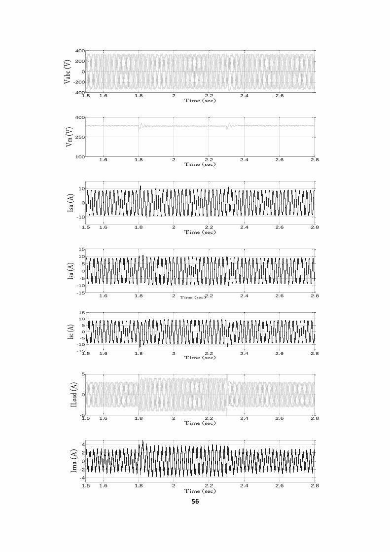
Fig. 3.7 depicts the performance characteristics of generator terminal voltage (𝑉𝑎𝑏𝑐), generator
line currents (𝐼𝑠𝑎 , 𝐼𝑠𝑏 , 𝐼𝑠𝑐 ), three phase ac load current (𝐼𝐿𝑜𝑎𝑑 𝑎𝑏𝑐 ), three phase STATCOM
currents (𝐼𝑚𝑎 , 𝐼𝑚𝑏 , 𝐼𝑚𝑐), peak value of generator terminal voltage (𝑉𝑝) and the reference value
(𝑉𝑝𝑟𝑒𝑓) of ac voltage and the dc capacitor voltage (𝑉𝑑𝑐) along with its reference value (𝑉𝑑𝑐𝑟𝑒𝑓)
of dc capacitor voltage. At 0.9 s an R-L load of 1.5 kW at 0.8 pf is connected which result in
fall of SEIG terminal voltage from its rated value. At 1.4 s gate pulses to IGBTs are given and
control action of STATCOM is activated. A small transient in SEIG terminal voltage is
observed with application of STATCOM. The generator supplies active power to STATCOM
to charge its dc bus capacitor to its reference voltage (700 V) and the capacitor act as a source
of reactive power to regulate terminal voltage of SEIG. The SEIG voltage again comes to its
rated voltage (410 V, line to line). The generator and STATCOM current increases to supply
active and reactive power as required by load.
0 0.5 1 1.5 2 2.5-4
-2
0
2
4
Time (sec)
Imc (
A)
0 0.5 1 1.5 2 2.50
200
400
600
800
Time (sec)
Vac
(V)
0 0.5 1 1.5 2 2.50
200
500
700
900
Time (sec)
Vdc
(V
)
Page 49
37
3.5.3 Performance of SEIG-STATCOM with PI Controller feeding Resistive Load
The transient performance of generator terminal voltage (𝑉𝑎𝑏𝑐) , generator line currents
( 𝐼𝑠𝑎 , 𝐼𝑠𝑏 , 𝐼𝑠𝑐 ), three phase load currents ( 𝐼𝑙𝑜𝑎𝑑 𝑎𝑏𝑐 ), three phase STATCOM current
(𝐼𝑚𝑎 , 𝐼𝑚𝑏 , 𝐼𝑚𝑐 ), peak of generator phase voltage (𝑉𝑝) with its reference value and dcapacitor
voltage (𝑉𝑑𝑐) with its reference voltage are illustrated in Fig. 3.8 for a resistive load of 1.5 kW.
2 2.2 2.4 2.6 2.8 3 3.2 3.4 3.6 3.8 4-400
-200
0
200
400
Time (sec)
Vab
c (V
)
2 2.4 2.8 3.2 3.6 40
100
200
300
400
Time (sec)
Vm
(V)
2 2.4 2.8 3.2 3.6 4-20
-10
0
10
20
Time (sec)
Isa
(A)
2 2.4 2.8 3.2 3.6 4-20
-10
0
10
20
Time (sec)
Isb
(A)
2 2.4 2.8 3.2 3.6 4-20
-10
0
10
20
Time (sec)
Isc (
A)
Page 50
38
Fig. 3.8 Performance characteristics of SEIG-STATCOM system with PI controller supplying resistive load
(The load increased from 1.5 kW to 2.5 kW at 2.8 s and decrease to 1.5 kW at 3.5 s)
2 2.4 2.8 3.2 3.6 4
-5
0
5
Time (sec)
I Loa
d (A)
2 2.4 2.8 3.2 3.6 4-6
-3
0
3
6
Time (sec)
Ima (
A)
2 2.4 2.8 3.2 3.6 4-6
-3
0
3
6
Time (sec)
Imb
(A)
2 2.4 2.8 3.2 3.6 4-6
-3
0
3
6
Time (sec)
Imc
(A)
2 2.4 2.8 3.2 3.6 3.8 4300
400
500
600
Time (sec)
Vac
(V)
2.8 3.2 3.6 3.8 4600
700
800
Time (sec)
Vdc
(V)
Page 51
39
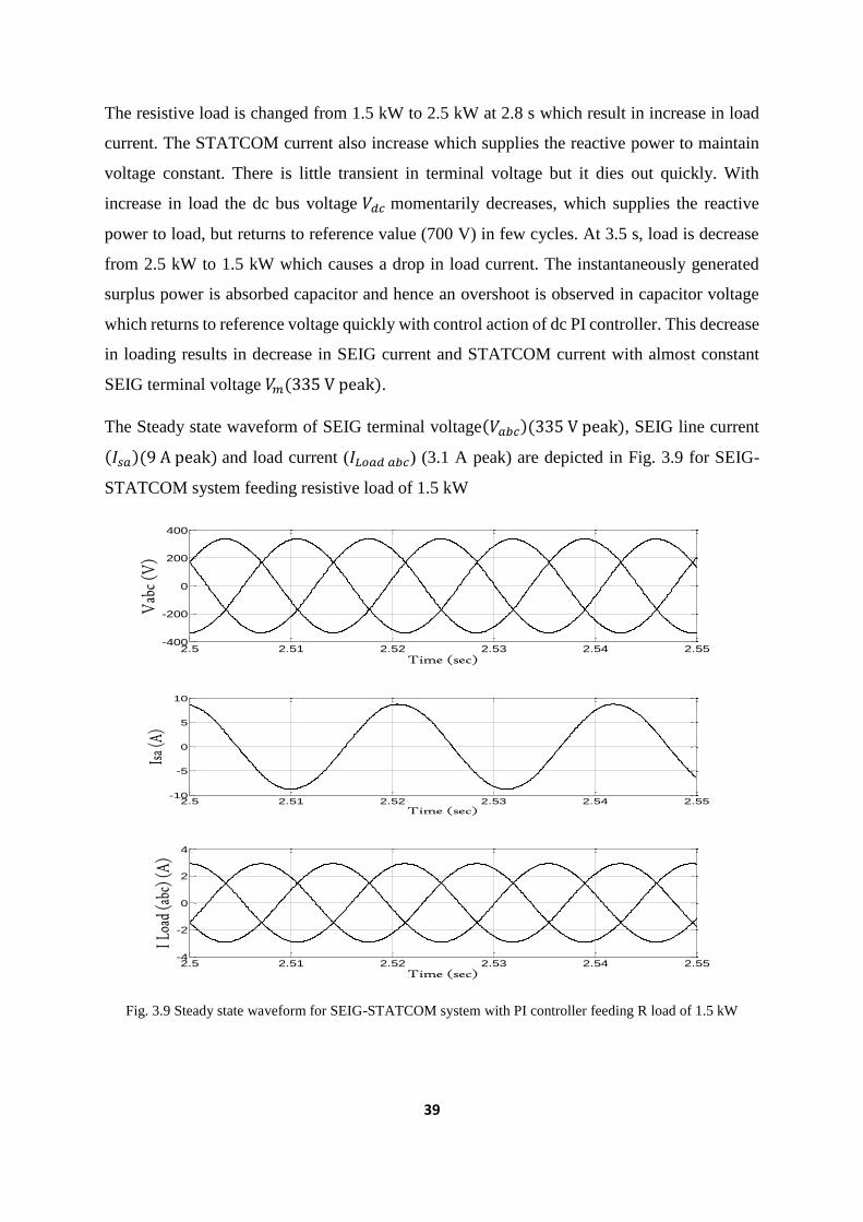
The resistive load is changed from 1.5 kW to 2.5 kW at 2.8 s which result in increase in load
current. The STATCOM current also increase which supplies the reactive power to maintain
voltage constant. There is little transient in terminal voltage but it dies out quickly. With
increase in load the dc bus voltage 𝑉𝑑𝑐 momentarily decreases, which supplies the reactive
power to load, but returns to reference value (700 V) in few cycles. At 3.5 s, load is decrease
from 2.5 kW to 1.5 kW which causes a drop in load current. The instantaneously generated
surplus power is absorbed capacitor and hence an overshoot is observed in capacitor voltage
which returns to reference voltage quickly with control action of dc PI controller. This decrease
in loading results in decrease in SEIG current and STATCOM current with almost constant
SEIG terminal voltage 𝑉𝑚(335 V peak).
The Steady state waveform of SEIG terminal voltage(𝑉𝑎𝑏𝑐)(335 V peak), SEIG line current
(𝐼𝑠𝑎)(9 A peak) and load current (𝐼𝐿𝑜𝑎𝑑 𝑎𝑏𝑐) (3.1 A peak) are depicted in Fig. 3.9 for SEIG-
STATCOM system feeding resistive load of 1.5 kW
Fig. 3.9 Steady state waveform for SEIG-STATCOM system with PI controller feeding R load of 1.5 kW
2.5 2.51 2.52 2.53 2.54 2.55-400
-200
0
200
400
Time (sec)
Vab
c (V
)
2.5 2.51 2.52 2.53 2.54 2.55-10
-5
0
5
10
Time (sec)
Isa (A
)
2.5 2.51 2.52 2.53 2.54 2.55-4
-2
0
2
4
Time (sec)
I Loa
d (a
bc) (
A)
Page 52
40
3.5.4 Performance of SEIG-STATCOM with PI Controller feeding R-L Load
The performance characteristics of SEIG-STATCOM system feeding a 0.8 pf R-L load is
shown in Fig. 3.10. Initially there is a load of 1.5 kW which changes to 2.2 kW.
2 2.4 2.8 3.2 3.6 4-400
-200
0
200
400
Time (sec)
Vab
c (V
)
2 2.4 2.8 3.2 3.6 4100
200
300
400
Time (sec)
Vm
(v)
2 2.4 2.8 3.2 3.6 4
-10
-5
0
5
10
Time (sec)
Isa
(A)
2 2.4 2.8 3.2 3.6 4
-10
-5
0
5
10
Time (sec)
Isb
(A)
2 2.4 2.8 3.2 3.6 4
-10
-5
0
5
10
Time (sec)
Isc
(A)
Page 53
41
Fig. 3.10 Performance analysis of SEIG-STATCOM system with PI controller feeding 0.8 pf R-L load
(Load is changed from 1.5 kW to 2.2 kW at 2.8 s and decrease to 1.5 kW at 3.5 s)
2 2.4 2.8 3.2 3.6 4-3
-2
-1
0
1
2
3
Time (sec)
I Lo
ad (
A)
2 2.4 2.8 3.2 3.6 4-4
-2
0
2
4
Time (sec)
Ima
(A)
2 2.4 2.8 3.2 3.6 4-4
-2
0
2
4
Time (sec)
Imb
(A)
2 2.4 2.8 3.2 3.6 4-4
-2
0
2
4
Time (sec)
Imc
(A)
2 2.4 2.8 3.2 3.6 4300
400
500
600
Time (sec)
Vac
(V)
2 2.4 2.8 3.2 3.6 3.8 4500
600
700
800
Time (sec)
Vdc
(V)
Page 54
42
Waveforms from top to bottom, respectively relates to generator terminal voltage(𝑉𝑎𝑏𝑐), line
currents (𝐼𝑠𝑎 , 𝐼𝑠𝑏 , 𝐼𝑠𝑐) of source, three phase load currents (𝐼𝑙𝑜𝑎𝑑 𝑎𝑏𝑐), three phase STATCOM
current (𝐼𝑚𝑎 , 𝐼𝑚𝑏 , 𝐼𝑚𝑐 ), peak value of generated terminal voltage (𝑉𝑝) along with its reference
value and capacitor voltage (𝑉𝑑𝑐) along with its reference voltage. The load is changed from
1 kW to 2.2 kW at 2.8 s which causes increase in load current. The generated terminal voltage
remains almost constant with small transients which quickly dies out. With increase in load the
compensation current (i.e. STATCOM current) increases which supplies the increase reactive
demanded by load. The SEIG current also increases which fulfil the active power requirement
as demanded with increase in load. A small change in peak voltage 𝑉𝑎𝑐 is observed, but it
returns to its reference voltage (581 V) after few cycles. The dc bus voltage 𝑉𝑑𝑐 also changes
with application of load, but quickly return to reference value (700 V). The load is again
reduced to 1.5 kW at 2.8 s which result in corresponding decrease in STATCOM currents and
SEIG currents. The surplus generated power is now absorbed by dc bus capacitor as a results
there is small variation in capacitor voltage, which settles to its reference value within few
cycle. With sudden decrease in load, the peak ac terminal voltage 𝑉𝑎𝑐 increases from its set
value and returns to reference value under PI control action.
Fig. 3.11 illustrates the steady-state waveforms of SEIG –STATCOM system depicting SEIG
terminal voltage(𝑉𝑎𝑏𝑐)(335 V peak), SEIG line current (𝐼𝑠𝑎)(7.3 A peak) and load current
waveform (𝐼𝐿𝑜𝑎𝑑 𝑎𝑏𝑐) (2 A peak) feeding 0.8 pf R-L load of 2.5 kW
3 3.01 3.02 3.03 3.04 3.05-400
-200
0
200
400
Time (sec)
Vab
c (V
)
3 3.01 3.02 3.03 3.04 3.05-10
-5
0
5
10
Page 55
43
Fig. 3.11 Steady state waveform for SEIG-STATCOM system with PI controller feeding 0.8 pf R-L load of
2.5 kW
3.5.5 Performance of SEIG-STATCOM with PI Controller feeding Non-linear load
(Three Phase Diode Rectifier with Resistive load)
The simulated waveforms of generator terminal voltage(𝑉𝑎𝑏𝑐), line currents (𝐼𝑠𝑎 , 𝐼𝑠𝑏 , 𝐼𝑠𝑐),
three phase load currents (𝐼𝑙𝑜𝑎𝑑 𝑎𝑏𝑐), three phase STATCOM current (𝐼𝑚𝑎, 𝐼𝑚𝑏 , 𝐼𝑚𝑐 ), peak of
ac terminal voltage (𝑉𝑝) along with its reference value and capacitor voltage (𝑉𝑑𝑐) along with
its reference voltage are illustrated in Fig. 3.12 for a three phase SEIG-STATCOM with PI
control feeding ta non-linear load.
3 3.01 3.02 3.03 3.04 3.05-3
-2
0
2
3
Time (sec)
I Loa
d (ab
c) (A
)
1.8 2 2.2 2.4 2.6 2.8 3
-400
-200
0
200
400
Time (sec)
Vab
c
1.8 2 2.2 2.4 2.6 2.8 30
100
200
300
400
Time (sec)
Vm
(V)
1.8 2 2.2 2.4 2.6 2.8 3-10
-5
0
5
10
Time (sec)
Isa
Page 56
44
1.8 2 2.2 2.4 2.6 2.8 3-10
0
10
Time (sec)
Isb
1.8 2 2.2 2.4 2.6 2.8 3-10
-5
0
5
10
Time (sec)
Isc
1.8 2 2.2 2.4 2.6 2.8 3
-3
0
3
Time (sec)
ILab
c
1.8 2 2.2 2.4 2.6 2.8 3-4
-2
0
2
4
Time (sec)
Ima
(A)
1.8 2 2.2 2.4 2.6 2.8 3-5
0
5
Time (sec)
Imb
(A)
1.8 2 2.2 2.4 2.6 2.8 3-5
0
5
Time (sec)
Imc
(A)
Page 57
45
Fig. 3.12 Performance characteristics of SEIG-STATCOM system with PI controller feeding a non-linear load
(A three phase diode rectifier with resistive load change from 2 kW to 1.5 kW at 2.5 s)
Waveforms from top to bottom, respectively refers to generator terminal voltage(𝑉𝑎𝑏𝑐), line
currents of source (𝐼𝑠𝑎, 𝐼𝑠𝑏 , 𝐼𝑠𝑐), three phase load currents (𝐼𝑙𝑜𝑎𝑑 𝑎𝑏𝑐), three phase STATCOM
current (𝐼𝑚𝑎 , 𝐼𝑚𝑏 , 𝐼𝑚𝑐 ), peak value of ac terminal voltage (𝑉𝑝) along with its reference value
and capacitor voltage (𝑉𝑑𝑐) along with its reference voltage. At 2.5 s, the resistive load on three
phase diode rectifier is decrease from 2 kW to 1.5 kW. This result in decrease in generator,
STATOR and load current to cut out the demand of reactive and active power to the load. With
reduction in load value, small transient is observed in capacitor voltage which fulfil the reactive
power demand of generator and load. The capacitor voltage settles to its reference value (700
V) within few cycles. With sudden decrease in load 𝑉𝑎𝑐 also increases from its set value and
returns to reference value under PI control action.
The Steady state waveform of SEIG terminal voltage (𝑉𝑎𝑏𝑐)(335 V peak) , load current
(𝐼𝐿𝑜𝑎𝑑 𝑎𝑏𝑐) (1.5 A peak) and SEIG line current (𝐼𝑠𝑎)(7.2 A peak) are depicted in Fig. 3.13 for
SEIG-STATCOM system feeding non-linear load.
1.8 2 2.2 2.4 2.6 2.8 3400
500
600
700
Time (sec)
Vac
1.8 2 2.2 2.4 2.6 2.8 3650
700
750
Time (sec)
Vdc
2 2.01 2.02 2.03 2.04 2.05-400
-200
0
200
400
Time (sec)
Vab
c (V
)
Page 58
46
Fig. 3.13 Steady state waveform for SEIG-STATCOM system with PI controller feeding three phase diode
rectifier with restive load of 2 kW
3.6 Conclusion
The modelling and simulation of SEIG with STATCOM have been carried out for linear and
non-linear loads using conventional PI control. The proposed scheme for regulating voltage of
SEIG is simple, efficient and easy to implement. From the simulated result, it has been found
that the terminal voltage of generator remains constant irrespective of load. Whenever load is
increased, either linear or non-linear, STATCOM supplies the compensated current for meeting
the reactive power as demanded by load. For supplying the active power to load the generator
current also increases. With decrease in load, the surplus generated power is absorbed by the
capacitor of dc bus. When three phase rectifier load is connected, the STATCOM balanced the
unbalanced load currents, and the generator currents but voltage remain balanced and
sinusoidal at its rated value. Hence STATCOM acts as a load balancer. The STATCOM also
eliminates the harmonics generated by non-linear load. Thus with application of STATCOM,
the voltage regulation of SEIG improves by injection of compensation currents. It is also
observed that the performance of conventional PI controller is quite satisfactory but it takes
more time to reach its steady state value and the steady state performance is not smooth.
2 2.01 2.02 2.03 2.04 2.05-2
-1
0
1
2
Time (sec)
I L
oad
(A)
2 2.005 2.01 2.015 2.02 2.025 2.03 2.035 2.04 2.045 2.05-10
-5
0
5
10
Time (sec)
Isa
(A)
Page 59
47
Chapter-4
MODELLING OF STATCOM BASED FUZZY VOLTAGE
CONTROLLER FOR SEIG DRIVEN BY CONSTANT SPEED
PRIME MOVER
4.1 General
Chapter-3 presents the modelling of STATCOM based voltage regulator for SEIG using
conventional PI control but voltage regulation using STATCOM with conventional PI control
has certain demerits [4]-[17]. The major demerit of conventional PI control requires
mathematical model of the system. The conventional PI control cannot handle non-linearity as
it is quite difficult to model a non-linear system. The conventional PI control are also sensitive
to parameter variation and they cannot work with imprecise and noisy input. The PI control has
poor dynamic response and noisy steady state response as seen in chapter 3. This chapter deals
with the modelling of STATCOM using Fuzzy controller with which eliminates all demerits
of conventional PI control [26]- [28].
This thesis illustrate the design of Mamdani type Fuzzy controller for STATCOM for
regulating the SEIG voltage. The merits of using Fuzzy controller system over conventional
PI system are as follows
a) Fuzzy control does not require exact mathematical model
b) Fuzzy controller is based on simple linguistic information and thus easy to understand
c) It does not require precise input, as it can work with imprecise and noisy input
d) Fuzzy controller is insensitive to parameter variation as it does not require accurate
mathematical model
e) Fuzzy controller offers more flexibility as it is easy to modify the functionality
4.2 Basic of Fuzzy Controller
Fig. 4.1 shows the basic inference system using fuzzy approach. Its major components are
input, fuzzy system, and output. The output is evaluated by aggregating all rules. We can
frame as many as rule depending on complexity of the system and its ease to implement.
Page 60
48
Fig. 4.1 Basic components of Fuzzy controller
Step I: Fuzzification
Fuzzy logic converts the numerical variables into linguistic variables. But the variables are
available are real numbers. The method of transforming a numerical variable (real number)
into linguistic variable is called fuzzification. It is the first step to select no. of inputs and assign
linguistic variables to each input and membership function to them with suitable numerical
values. The membership functions are represented by different shapes such as triangular,
trapezoidal, Gaussian, etc. but generally triangular is used because of its simplicity.
Step II: Formation of rule base
This step form the rule of controller to control the action taken from knowledge of control rules
and linguistic variable. It has three different components as follows
a) IF (predecessor and antecedent) –use of fuzzy operator in it.
b) THEN part of rule-suggestion or inference from antecedent part to the subsequent part.
c) Aggregation (accumulation) of the subsequent of all rules.
For decision making a specific set of rule base are formed which is based on human thinking
in the form of IF-THEN rule. Then these rules can be aggregated using OR or AND operator.
A total of (𝑚 × 𝑛) rules can be formed based on combinations of different inputs, where m is
no. of inputs and n is number of membership functions for each inputs. Suppose that there are
two inputs, input 1 has two membership function and input 2 has three membership functions,
then a total of 6 rules can be framed.
Fuzzification Defuzzification
Rule base/ Decision making
Inputs Output
Fuzzy Logic System
Page 61
49
Step III: Decision making
The rule framed above is required to be processed to take decision based on input information
available. Fuzzy operator OR (MAX) is used to process the ‘then’ part. The And (MIN) can
also be used. The various operators of Fuzzy logic are described below
1. AND- Intersection: 𝜏𝐴∩𝐵(𝑥) = min [𝜏𝐴(𝑥), 𝜏𝐵(𝑥)]
2. OR-Union: 𝜏𝐴∩𝐵(𝑥) = max [𝜏𝐴(𝑥), 𝜏𝐵(𝑥)]
3. NOT-Complement: 𝜏𝐴(𝑥) = 1-𝜏𝐴(𝑥)
Where 𝜏𝐵(𝑥) and 𝜏𝐵(𝑥) denote the degree of membership function of given element in fuzzy
sets A and B
Step IV: Defuzzification
This is the conversion of linguistic fuzzy control variables to a non-fuzzy control action. The
truncated output MFs obtained after implication of each rule are combined or aggregated to
obtain final fuzzy output. The fuzzy output obtained after aggregation is converted to crispy
value. This step is known as defuzzification. One method of defuzzification is finding centroid
or centre of gravity of the area.
4.3 Modelling of STATCOM with Fuzzy Logic Controller
Recently, Fuzzy logic controllers have gained more attention and extensively used in various
power electronic applications. The advantage of Fuzzy controllers over conventional PI
controllers is that they don’t require an exact mathematical model of the system and can work
with imprecise and noisy inputs [18-19]. The conventional PI control take more time for
computation as it takes more time for the settling of dc capacitor voltage. Therefore there is
need to track the dc voltage to its reference value as fast as possible for better dynamic response.
In this work, Mamdani type fuzzy controller has been implemented for STATCOM, which
reduces the settling time of capacitor voltage waveform and reduces Total Harmonic
Distortion. In this thesis through simulation result, it has been shown that Mamdani type fuzzy
controller has improve the dynamic response of the system and has smooth steady state
performance as compared to conventional PI control. The performance characteristics of Fuzzy
logic controller is more robust and better than conventional PI controller with variation of load
and parameter variations.
Page 62
50
Fig. 4.2 Fuzzy control scheme for capacitor voltage control
Fig. 4.2 illustrates the fuzzy control scheme used in place of conventional PI control for
capacitor voltage. The capacitor voltage (𝑉𝑑𝑐) is sensed from dc bus capacitor and compared
with capacitor voltage (𝑉𝑑𝑐𝑟𝑒𝑓 , 700 V). The error signal generated from the difference of
reference dc voltage and actual dc voltage is amplified. In case of fuzzy logic control scheme
error (e) and change in error (ce(n) = e(n)-e(n-1)) are used as inputs for fuzzy controller. The
output of fuzzy logic controller is amplified and taken as peak of d-axis current (𝑖𝑠𝑚𝑑∗ ) which
multiplied with in-phase component of current (𝑢, 𝑢𝑏 , 𝑢𝑐) to give d-axis reference currents
(𝑖𝑠𝑎𝑑∗ , 𝑖𝑠𝑏𝑑
∗ , 𝑖𝑠𝑐𝑑∗ ).
A memory block is used to calculate the change in error (ce) which gives one integration step
delay. The characteristics of fuzzy controller used are as follows
a) Seven memebership functions are used for each input (e and ce) and output
b) Triangular functions are used for simplicity
c) Implication is done using Mamdani’s ‘min’ operator
d) Defuzzification using ‘Centre of Area (COA)’ method
The seven member ship functions used for each input and output are as follows
a) BN-Big Negative
b) MN-Medium Negative
c) SN-Small Negative
d) ZE-Zero
e) SP-Small Positive
f) MP-Medium Positive
Vdcref
Vdc
Gain
K dc1 Kdc2
Error (e)
Change inerror (ce)
Fuzzy LogicController
(Rule Base)
STATCOM
Gain
+
-
+-
Memory
(700 V)
Page 63
51
g) BP- Big Psitive
Thus a total of 49 (7×7) are framed as given in Table 1 below
ce / e BN MN SN ZE SP MP BP
BN BP BP BP BP MP SP ZE
MN BP BP BP MP SP ZE SN
SN BP BP MP SP ZE SN MN
ZE BP MP SP ZE SN MN BN
SP MP SP ZE SN MN BN BN
MP SP ZE SN MN BN BN BN
BP ZE SN MN BN BN BN BN
Table 1. Rule base table of fuzzy controller for STATCOM
Similarly for ac voltage control same method is adopted and control circuit is depicted in Fig.
4.3
Fig. 4.3 Fuzzy control scheme for ac peak voltage control
Fig. 4.3 shows the fuzzy control scheme used for controlling the peak ac voltage in place of
conventional PI control. The peak terminal voltage (𝑉𝑝) is sensed reference ac voltage (𝑉𝑝𝑟𝑒𝑓,
581 V) are fed to comparator. The output of ac fuzzy controller is amplified and taken as peak
of q-axis current (𝑖𝑠𝑚𝑞∗ ) which multiplied with quadrature component (𝑤𝑎, 𝑤𝑏 , 𝑤𝑐) of current
to give q-axis reference currents (𝑖𝑠𝑎𝑞∗ , 𝑖𝑠𝑏𝑞
∗ , 𝑖𝑠𝑐𝑞∗ ). The rule base for ac fuzzy controller is same
as of dc fuzzy controller. The d-axis reference current templates (𝑖𝑠𝑎𝑑∗ , 𝑖𝑠𝑏𝑑
∗ , 𝑖𝑠𝑐𝑑∗ ) and q-axis
Vpref
Vp
Gain
K ac1 Kac2
Error (e)
Change inerror (ce)
Fuzzy LogicController
(Rule Base)
STATCOM
Gain
+
-
+-
Memory581 V
Page 64
52
reference currents templates (𝑖𝑠𝑎𝑞∗ , 𝑖𝑠𝑏𝑞
∗ , 𝑖𝑠𝑐𝑞∗ ) are added to give three phase (𝑖𝑠𝑎
∗ , 𝑖𝑠𝑏∗ , 𝑖𝑠𝑐
∗ ) source
reference currents. By comparing actual source currents (𝑖𝑠𝑎, 𝑖𝑠𝑏 , 𝑎𝑛𝑑 𝑖𝑠𝑐 ) with m source
reference current templates the gate pulse for switches are generated.
4.4 Simulation of SEIG-STACOM with Fuzzy Logic Control in MATLAB/SIMULINK
The model of SEIG-STATCOM with fuzzy Control is simulated in MATLAB/Simulink
environment. Initially SEIG is allowed to induce its terminal voltage by excitation capacitors.
Then STATCOM is connected to SEIG but pulses to VSI controller is not given. The dc bus
capacitor gets charges to SEIG terminal voltage value. Then load is connected which reduces
the SEIG terminal voltage, after that gate pulses are given to switches of VSI and voltage is
restored to their initial values. The values of various parameters of STATCOM is given below.
𝐿𝑓(H) 𝐶𝑑𝑐(F) 𝐾𝑎𝑐1 𝐾𝑎𝑐2 𝐾𝑑𝑐1 𝐾𝑑𝑐2
50e-3 200e-6 1/8700 498 1/1400 310
For simulation a 3.7kW, 415V, 7.5A, 4-Pole, 3-phase squirrel cage induction machine is used
as generator. Different transient waveforms are illustrated to depict the performance of
proposed voltage control scheme supplying balanced/unbalanced linear/non-linear load. The
result under various conditions are discussed below.
4.5 Result and Discussion
4.5.1 Voltage build-up of SEIG, Connection of Load and Switching of Gate Pulses for R
Load
Fig. 4.4 illustrates the performance characteristics of SEIG-STATCOM with fuzzy logic
controller feeding a purely resistive load of 1.5 kW. Initially SEIG is at no load and allowed to
build-up its terminal voltage through excitation capacitors. Then STATCOM is connected but
gate pulses to IGBTs are not given. Then load is switched on which causes the fall in terminal
voltage of SEIG. Now the gate pulses are given to switches which restore the SEIG terminal
voltage to its rated value.
Page 65
53
0 0.2 0.4 0.6 0.8 1 1.2 1.4 1.6 1.8 2-400
-200
0
200
400
Time (sec)
Vab
c
0 0.2 0.4 0.6 0.8 1 1.2 1.4 1.6 1.8 20
150
300
450
Time (sec)
Vm
0 0.2 0.4 0.6 0.8 1 1.2 1.4 1.6 1.8 2-10
-5
0
5
10
Time (sec)
Isa
0 0.2 0.4 0.6 0.8 1 1.2 1.4 1.6 1.8 2
-10
0
10
Time (sec)
Isb
0 0.2 0.4 0.6 0.8 1 1.2 1.4 1.6 1.8 2-10
-5
0
5
10
Time (sec)
Isc
0 0.2 0.4 0.6 0.8 1 1.2 1.4 1.6 1.8 2-4
-2
0
2
4
Time (sec)
I Loa
d (A
)
0 0.2 0.4 0.6 0.8 1 1.2 1.4 1.6 1.8 2-4
-2
0
2
4
Time (sec)
Ima
(A)
Page 66
54
Fig. 4.4 Performance analysis of SEIG-STATCOM with Fuzzy Controller feeding R load of 1.5 kW
(at 0.6 s STATCOM is connected, load is connected at 0.95 s and gate pulses given at 1.4 s)
Response from top to bottom, respectively refers to generator terminal voltage (𝑉𝑎𝑏𝑐), peak
value of terminal ac phase voltage (𝑉𝑚), SEIG line currents (𝐼𝑠𝑎, 𝐼𝑠𝑏 , 𝐼𝑠𝑐), three phase ac load
current (𝐼𝐿𝑜𝑎𝑑 𝑎𝑏𝑐), three phase STATCOM currents (𝐼𝑚𝑎 , 𝐼𝑚𝑏 , 𝐼𝑚𝑐), peak of SEIG terminal
voltage (𝑉𝑝) along with its reference value (𝑉𝑝𝑟𝑒𝑓) and capacitor voltage (𝑉𝑑𝑐) along with its
reference value (𝑉𝑑𝑐𝑟𝑒𝑓). First voltage is build up and then STATCOM is connected. The dc
bus capacitor gets charged to peak of ac line voltage (581 V) through antiparallel diodes. The
load is connected at 0.95 s which decreases the SEIG terminal voltage (𝑉𝑎𝑏𝑐). At 1.4 s gate
pulses are applied to IGBTs of VSI and SEIG voltage returns to its rated value of 335 V (peak
phase voltage). The STATCOM supplies the compensating current at 1.4 s which is responsible
0 0.2 0.4 0.6 0.8 1 1.2 1.4 1.6 1.8 2-4
-2
0
2
4
Time (sec)
Imb
(A)
0 0.2 0.4 0.6 0.8 1 1.2 1.4 1.6 1.8 2-4
-2
0
2
4
Time (sec)
Imc
(A)
0 0.2 0.4 0.6 0.8 1 1.2 1.4 1.6 1.8 20
200
400
600
Time (sec)
Vac
(V
)
0 0.2 0.4 0.6 0.8 1 1.2 1.4 1.6 1.8 20
200
400
600
800
Time (sec)
Vdc
(V
)
Page 67
55
fulfilling the reactive power requirement of load and regulate the SEIG terminal voltage. The
SEIG currents also increases to provide active power requirement of load.
The Steady state waveform of SEIG terminal voltage (𝑉𝑎𝑏𝑐)(335 V peak) , load current
(𝐼𝐿𝑜𝑎𝑑 𝑎𝑏𝑐) (3.1 A peak) and SEIG line current (𝐼𝑠𝑎)(9 A peak) are depicted in Fig. 4.5 for
SEIG-STATCOM system with Fuzzy controller during switching in STACOM feeding
resistive load of 1.5 kW.
Fig. 4.5 Steady state waveform for SEIG-STATCOM system with Fuzzy controller feeding R load of 1.5 kW
4.5.2 Performance of SEIG-STATCOM with Fuzzy Logic Control feeding R Load
The performance characteristics of generator terminal voltage(𝑉𝑎𝑏𝑐), peak value of terminal
phase voltage (𝑉𝑚), generator line currents (𝐼𝑠𝑎 , 𝐼𝑠𝑏 , 𝐼𝑠𝑐), three phase load currents (𝐼𝑙𝑜𝑎𝑑 𝑎𝑏𝑐),
three phase STATCOM current (𝐼𝑚𝑎, 𝐼𝑚𝑏 , 𝐼𝑚𝑐 ), peak of generator terminal voltage (𝑉𝑝) along
with its reference value and dc capacitor voltage (𝑉𝑑𝑐) along with its reference voltage are
illustrated in Fig. 4.6 feeding resistive load with Fuzzy logic controller.
1.6 1.61 1.62 1.63 1.64-500
0
500
Time (sec)
Vab
c (V
)
1.6 1.61 1.62 1.63 1.64-5
0
5
Time (sec)
I lo
ad (
A)
1.6 1.61 1.62 1.63 1.64-10
0
10
Time (sec)
Isa
(A)
Page 68
56
1.5 1.6 1.8 2 2.2 2.4 2.6-400
-200
0
200
400
Time (sec)
Vab
c (V
)
1.6 1.8 2 2.2 2.4 2.6 2.8100
250
400
Time (sec)
Vm
(V)
1.5 1.6 1.8 2 2.2 2.4 2.6 2.8
-10
0
10
Time (sec)
Isa
(A)
1.6 1.8 2 2.2 2.4 2.6 2.8-15
-10
-5
0
5
10
15
Time (sec)
Isa (
A)
1.5 1.6 1.8 2 2.2 2.4 2.6 2.8-15
-10
-5
0
5
10
15
Time (sec)
Isc (A
)
1.5 1.6 1.8 2 2.2 2.4 2.6 2.8-5
0
5
Time (sec)
ILoa
d (A
)
1.5 1.6 1.8 2 2.2 2.4 2.6 2.8
-4
-2
0
2
4
Time (sec)
Ima
(A)
Page 69
57
Fig. 4.6 Performance analysis of SEIG-STATCOM system with Fuzzy controller supplying resistive load
(Load is changed from 1.5 kW to 2.5 kW at 1.8 s and decrease to 1.5 kW at 2.3 s)
Initially there is 1.5 kW resistive load which changes to 2.5 kW at 1.8 s. With increase in load,
load current also changes. Under load change the terminal voltage of generator remains
constant with small transient in waveform which dies out quickly. The STATCOM and SEIG
current further increases to supply active and reactive power as demanded by load respectively.
There is small transient in the dc bus voltage with application of load, but it returns to its
reference value within few cycles. At 2.3 s load is again decrease to 1.5 kW. With sudden
increase in generated power, the dc bus capacitor absorbs the surplus generated power and thus
STATCOM current decreases. The SEIG current also decreases in order to supply active power
demand of load. The small transient is present in dc bus voltage with decrease in load which
returns to its reference value after few cycles. The ac peak voltage also deviates from its
reference value with sudden change in load but it quickly returns to its reference value under
Fuzzy logic control.
1.5 1.6 1.8 2 2.2 2.4 2.6 2.8-5
0
5
Time (sec)
Imb
( A)
1.5 1.6 1.8 2 2.2 2.4 2.6 2.8-4
-2
0
2
4
Time (sec)
Imc (
A)
1.6 1.8 2 2.2 2.4 2.6 2.8
600
400
200
Time (sec)
Vac
(V
)
1.6 1.8 2.0 2.2 2.6 2.8500
600
700
800
Time (sec)
Vdc
(V)
Page 70
58
The Steady state waveform of SEIG terminal voltage (𝑉𝑎𝑏𝑐)(335 V peak) , load current
(𝐼𝐿𝑜𝑎𝑑 𝑎𝑏𝑐) (5 A peak) and SEIG line current (𝐼𝑠𝑎)(10 A peak) are depicted in Fig. 4.7 for
SEIG-STATCOM system with Fuzzy controller feeding resistive load of 2.5 kW.
Fig. 4.7 Steady state waveform for SEIG-STATCOM system with Fuzzy controller feeding R load of 2.5 kW
4.5.3 Performance of SEIG-STATCOM with Fuzzy Logic Control feeding R-L Load
The simulated waveforms of SEIG-STATCOM with Fuzzy controller for R-L load at 0.8 pf is
depicted in Fig. 4.8. Initially there is a load of 1.5 kW which changes to 2.2 kW.
1.9 1.91 1.92 1.93 1.94-400
-200
0
200
400
Time (sec)
Vab
c (V
)
1.9 1.91 1.92 1.93 1.94
-5
0
5
Time (sec)
I Loa
d (A
)
1.9 1.91 1.92 1.93 1.94
-10
0
10
Time (sec)
Isa
(A)
1.6 1.8 2 2.2 2.4 2.6-500
0
500
Time (sec)
Vab
c (V
)
Page 71
59
1.6 1.8 2 2.2 2.4 2.6100
200
300
400
Time (sec)
Vm
(V)
1.6 1.8 2 2.2 2.4 2.6
-10
0
10
Time (sec)
Isa
(A)
1.6 1.8 2 2.2 2.4 2.6
-10
0
10
Time (sec)
Isb
(A)
1.6 1.8 2 2.2 2.4 2.6
-10
0
10
Time (sec)
Isc
(A)
1.6 1.8 2 2.2 2.4 2.6-4
-2
0
2
4
Time (sec)
I Loa
d (A
)
1.6 1.8 2 2.2 2.4 2.6
-4
-2
0
2
4
Time (sec)
Ima
(A)
1.6 1.8 2 2.2 2.4 2.6
-4
-2
0
2
4
Time (sec)
Imb
(A)
Page 72
60
Fig. 4.8 Performance analysis of SEIG-STATCOM with Fuzzy Controller feeding R-L load of 0.8 pf
(Load is changed from 1.5 kW to 2.2 kW at 1.8 s and decrease to 1.5 kW at 2.2 s)
Fig. 4.8 shows the transient waveforms of generator terminal voltage(𝑉𝑎𝑏𝑐), peak value of
terminal phase voltage (𝑉𝑚), generator line currents (𝐼𝑠𝑎 , 𝐼𝑠𝑏 , 𝐼𝑠𝑐), three phase load currents
(𝐼𝑙𝑜𝑎𝑑 𝑎𝑏𝑐), three phase STATCOM current (𝐼𝑚𝑎 , 𝐼𝑚𝑏 , 𝐼𝑚𝑐 ), peak of ac terminal voltage (𝑉𝑝)
along with its reference value and capacitor voltage (𝑉𝑑𝑐) along with its reference voltage for
Fuzzy controller feeding R-L load of 0.8 pf. At 1.8 s load is increased from 1.5 kW to 2.2 kW.
Consequently, the generator and STATCOM currents are increases to provide the active and
reactive power demand of load. The load current also increases with increase in load. With
sudden increase in load an undershoot is observed in capacitor voltage of STATCOM, which
supplies necessary reactive power demand of load and generator, to maintaining the SEIG
terminal voltage constant. This variation in capacitor voltage settles to its reference value (700
V) after few cycles. At 2.2 s load is again decreased from 2.2 kW to 1.5 kW. The dc bus
capacitor absorbed the surplus generated voltage and as a result the STACOM and generator
line current decreases but SEIG terminal voltage remains constant at its rated value (335 V).
The ac peak voltage also deviates from its reference value with decrease in load but it quickly
returns to its reference value due to Fuzzy logic control.
1.6 1.8 2 2.2 2.4 2.6
-4
-2
0
2
4
Time (sec)
Imc
(A)
1.5 1.8 2.0 2.2 2.4 2.6400
500
600
700
Time (sec)
Vac
(V)
1.5 1.8 2.0 2.2 2.4 2.6500
600
700
800
Time (s)
Vdc
(V
)
Page 73
61
Fig. 4.9 illustrates the steady-state waveforms of SEIG –STATCOM system depicting SEIG
terminal voltage(𝑉𝑎𝑏𝑐)(335 V peak), SEIG line current (𝐼𝑠𝑎)(7.1 A peak) and load current
waveform (𝐼𝐿𝑜𝑎𝑑 𝑎𝑏𝑐) (1.5 A peak) feeding 0.8 pf R-L load of 1.5 kW
Fig. 4.9 Steady state waveforms of SEIG-STATCOM with Fuzzy Controller feeding 0.8 pf R-L load of 1.5 kW
4.5.4 Performance of SEIG-STATCOM with Fuzzy Logic Control feeding Non-linear
load (Three Phase Diode Rectifier with Resistive load)
The simulated waveforms of generator terminal voltage (𝑉𝑎𝑏𝑐), peak value of terminal phase
voltage (𝑉𝑚), generator line currents (𝐼𝑠𝑎, 𝐼𝑠𝑏 , 𝐼𝑠𝑐), three phase load currents (𝐼𝑙𝑜𝑎𝑑 𝑎𝑏𝑐), three
phase STATCOM current (𝐼𝑚𝑎, 𝐼𝑚𝑏 , 𝐼𝑚𝑐 ), peak of ac terminal voltage (𝑉𝑝 ) and capacitor
voltage (𝑉𝑑𝑐) for SEIG-STATCOM system with Fuzzy logic control feeding three phase diode
rectifier with resistive load is shown in Fig. 4.10
1.6 1.61 1.62 1.63 1.64-400
-200
0
200
400
Time (sec)
Vab
c (V
)
1.6 1.61 1.62 1.63 1.64-2
0
2
Time (sec)
I L
oad
(A
)
1.6 1.61 1.62 1.63 1.64 1.65-10
0
10
Time (sec)
Isa
(A)
Page 74
62
1.6 1.8 2 2.2 2.4 2.6-500
0
500
Time (sec)
Vab
c (V
)
1.6 1.8 2 2.2 2.4 2.6100
200
300
400
Time (sec)
Vm
(V)
1.6 1.8 2 2.2 2.4 2.6-10
0
10
Time (sec)
Isa
(A)
1.6 1.8 2 2.2 2.4 2.6-10
-5
0
5
10
Time (sec)
Iba
(A)
1.6 1.8 2 2.2 2.4 2.6-10
0
10
Time (sec)
Isc
(A)
1.6 1.8 2 2.2 2.4 2.6-4
-2
0
2
4
Time (sec)
ILa
(A)
1.6 1.8 2 2.2 2.4 2.6-4
-2
0
2
4
Time (sec)
Ima
(A)
Page 75
63
Fig. 4.10 Performance characteristics of SEIG-STATCOM system with Fuzzy controller feeding diode rectifier
with R load is decrease from 2 kW to 1.5 kW at 1.8 s and increase from 1.5 kW to 2 kW at 2.2 s
Response from top to bottom, respectively refers to generator voltage (𝑉𝑎𝑏𝑐), peak value of
terminal phase voltage (𝑉𝑚 ), SEIG line currents (𝐼𝑠𝑎, 𝐼𝑠𝑏 , 𝐼𝑠𝑐 ), three phase ac load current
(𝐼𝐿𝑜𝑎𝑑 𝑎𝑏𝑐 ), three phase STATCOM currents (𝐼𝑚𝑎, 𝐼𝑚𝑏 , 𝐼𝑚𝑐), peak value of SEIG terminal
voltage (𝑉𝑝) along with its reference value (𝑉𝑝𝑟𝑒𝑓) and capacitor voltage (𝑉𝑑𝑐) along with its
reference value (𝑉𝑑𝑐𝑟𝑒𝑓) for SEIG-STATCOM system feeding a non-linear load. At 1.8 s the
resistive load on three phase rectifier is decrease from 2 kW to 1.5 kW. With decrease in the
load the terminal voltage of generator remains constant but load current decreases. The dc bus
capacitor absorbs the surplus generated power as a result of which a overshoot is observed in
capacitor voltage, which tracks down to its reference voltage with in few cycles due to Fuzzy
control action. At 2.2 the resistive load on three phase diode rectifier is further increased from
1.5 kW to 2 kW. With increase in load, the STACOM, generator and load current also increases
to provide the necessary active and reactive powers to load. Due to increase in load an
1.6 1.8 2 2.2 2.4 2.6-4
-2
0
2
4
Time (sec)
Imb
(A)
1.6 1.8 2 2.2 2.4 2.6-4
-2
0
2
4
Time (sec)
Imc
(A)
1.5 1.8 2.0 2.2 2.4 2.6300
400
500
600
700
Time (sec)
Vac
(V)
1.5 1.8 2.0 2.2 2.4 2.6500
600
700
800
Time (sec)
Vd
c (V
)
Page 76
64
undershoot is observed in capacitor voltage which returns to its reference value within few
cycles under Fuzzy control action.
The Steady state waveform of SEIG terminal voltage (𝑉𝑎𝑏𝑐 − 335 V peak) , load current
(𝐼𝐿𝑜𝑎𝑑 𝑎𝑏𝑐 -2 A peak) and SEIG line current (𝐼𝑠𝑎 − 9 A peak) are depicted in Fig. 4.11 for
SEIG-STATCOM system feeding non-linear load.
Fig. 4.11 Steady state waveforms of SEIG-STATCOM with Fuzzy Controller feeding three phase diode rectifier
with resistive load of 2 kW
Fig. 4.12 depicts the response of dc bus capacitor voltage of conventional PI controller and
Fuzzy controller. From the response it is observed that the performance of PI controller and
Fuzzy controller are quite satisfactory. But fuzzy logic controller attain steady state value in
nearly 0.3 s whereas PI controller attains steady state value after 0.8 s. the peak overshoot in
dc voltage is 890 V in case of PI control while in Fuzzy control, it is 785 V. The settling time
of Fuzzy logic controller is less than conventional PI control and steady state response of Fuzzy
controller is much smoother as compared to PI control i.e. fuzzy control nearly maintains the
steady state value as constant as possible.
1.6 1.61 1.62 1.63 1.64 1.65-400
-200
0
200
400
Time (sec)
Vab
c (V
)
1.6 1.61 1.62 1.63 1.64 1.65-2
0
2
Time (sec)
I L
oad
(A)
1.6 1.61 1.62 1.63 1.64 1.65-10
0
10
Time (sec)
Isa
(A)
Page 77
65
Fig. 4.12 DC bus capacitor voltage during switch on response
4.6 Conclusion
The modelling and simulation of SEIG-STATCOM system using Fuzzy controller has been
carried out for both linear and non-linear loads. From the simulation results, it is clear that
Fuzzy controller gives better performance than PI controller under various load conditions. The
Fuzzy controller has less settling time, fast dynamic response and small peak overshoot as
compared to conventional PI control. Thus the implementation of Fuzzy controller instead of
PI controller is more beneficial and easy to use.
0 0.2 0.4 0.6 0.8 1 1.2
300
500
700
900
Time (sec)
Vd
cPI Control
FuzzyControl
Page 78
66
Chapter-5
MAIN CONCLUSION AND SCOPE FOR FUTURE WORK
5.1 Main Conclusion
The research work presented in the thesis mainly deals with analysis and development of fuzzy
and PI voltage controller for self-excited induction generator based on STATCOM. The
modelling and simulation of SEIG-STATCOM has been carried out for different types of loads.
The MATLAB based model of SEIG is developed in q and d stationary reference frame. The
SEIG develops its terminal voltage with the help of excitations capacitors. But with application
of load, terminal voltage falls down from its rated value. A STACOM based voltage regulator
is developed for regulating the SEIG voltage in MATLAB. The proposed scheme for
maintaining the voltage of SEIG constant is simple and easy to implement. The STATCOM
improves the voltage regulation by injection of compensation currents. The STATOM is design
for various loads like linear/ non-linear, balanced/unbalanced. From the simulation result it has
been found that the non-linear load injects harmonics in the system, which are also eliminated
by STATCOM. Hence it is concluded that STATCOM can act as voltage regulator, load
balancer and harmonic eliminator. In designing of STATCOM, PI and Fuzzy controllers are
used and their simulation result are compared. The Fuzzy controller based STATCOM gives
better dynamic performance. From the simulation result it is also found that the Fuzzy
controller has less peak overshoot, fast response and smooth steady state response as compared
to conventional PI control. Hence SEIG-STATCOM with fuzzy controller is a good candidate
for improving the performance of the regulator.
5.2 Scope for future work
The voltage regulation of self-excited induction generator using STATCOM have been
investigated for various loads (linear/non-linear) with PI and Fuzzy controller for improving
the performance of SEIG in standalone application. However further research work can be
carried out for better operation of SEIG. The areas in which further work can be done are as
follows
Page 79
67
1) The SEIG-STATCOM system can be developed for dynamic load also which increases
the flexibility of controller as it can be used for any type of load either linear or non-
linear, static or dynamic, balanced or unbalanced.
2) The STATCOM based controller can be developed for three phase SEIG feeding single
phase load using Fuzzy logic controller because fuzzy controller gives better dynamic
response as compared to PI controller.
3) Voltage regulation for SEIG driven by variable speed prime movers using STACOM
can be developed.
4) In standalone application using wind energy conversion system, the performance of
STATCOM based controller may be investigated using maximum power point
tracking.
Page 80
68
REFERENCES
[1] E. D. Basset and E. M. Potter, “Capacitive excitation for induction generator,” AIEE Trans.
On Electrical Engineering, vol. 54, pp. 540-545, May 1935.
[2] C. F. Wagner, “Process of self-excitation of induction motors,” AIEE Trans. On Electrical
Engineering, vol. 58, pp. 47-51, February 1939.
[3] J. E. Barkle and R. W. Ferguson, “Induction Generator theory and application,” AIEE
Trans. on Electrical Engineering, vol. 73, pp. 12-19, January 1954.
[4] A. S. Langdorf, Theory of Alternating current machinery, 2nd Ed. New York, McGraw-
Hill, 1995
[5] B. C. Doxey, “Theory and application of the capacitor excited induction generator,” The
Engineer, vol. 216, pp. 893-897, 1963.
[6] A. K. Tandon, “Investigations on the phenomenon of capacitor self-excitation in induction
machine and its applications,” Ph. D. Thesis, Dept. of Electrical Engineering, IIT Delhi, India,
1984.
[7] D. Levy, “Stand alone induction generators,” Electric Power System Research, vol. 41, pp.
191-201, 1997.
[8] A. K. Tandon, S. S. Murthy and G. J. Berg, “Steady state analysis of capacitor self-excited
induction generator,” IEEE Trans. on Power Apparatus and Systems, vol. 103, pp. 612-617,
March 1984.
[9] A. K. Tandon, S. S. Murthy and C. S. Jha, “New method of computing steady state response
of capacitor self-excitation induction generator,” Institution of Engineers, India, vol. 65, pp.
196-201, June 1985.
[10] N. H. Malik and S. E. Haque, “Steady state analysis and performance of an isolated self-
excited induction generator,” IEEE Trans. on Energy Conversion, vol. 1, pp. 134-139,
September 1986.
[11] P. C. Krause, Analysis of electric machinery, McGraw-Hill Book Co, New York, 1987.
Page 81
69
[12] D. W. Novotny, D. J. Gritter, “Self-excitation in inverter driven induction machine,” IEEE
Trans. on Power Apparatus and Systems, vol. 96, pp. 1117-1125, July-1997.
[13] N. H. Malik and A. Bahrain, “Influence of terminal capacitor on the performance
characteristics of self-excited induction generator,” IEE Trans. on Generation, Transmission
and Distribution, vol. 137, no. 2, pp. 168-173, March 1990.
[14] L. Wang and L. C. Huei, “A novel analysis on the performance of an isolated self-excited
induction generator,” IEEE Trans. on Energy Conversion, vol. 12, no. 2, pp. 109-117, June
1997.
[15] D. Seyoum, C. Grantham and M.F. Rahman, “The dynamic characteristics of an isolated
generator driven by a wind turbine,” IEEE Trans. on Industry Applications, vol. 39, no.4, pp.
936-944, July 2003.
[16] M. B. Brennen and A. Abbondanti, “Static exciters for induction generators,” IEEE Trans.
on Industry Applications, vol.13, no. 5, pp. 422-428, September 1977.
[17] B. Singh, S. S. Murthy and S. Gupta, “Transient analysis of self-excited induction
generator with electronic load controller (ELC) supplying static and dynamic loads,” IEEE
Trans. on Industry Applications, vol. 41, no. 5, pp. 1194-1204, September 2006
[18] B. Singh, S. S. Murthy and S. Gupta, “Analysis and design of electronic load controller
for self-excited induction generators,” IEEE Trans. on Energy Conversion, vol. 21, no.1, pp.
285-293, March 2006
[19] J. M. Ramirez and M. E. Torres, “An electronic load controller for the self-excited
induction generator,” IEEE Trans. on Energy Conversion., vol. 22, no.2, pp. 546-548, June
2007.
[20] A.C. Lopes and G.A. Rogerio, “Wind-driven self-excited induction generator with
voltage and frequency Regulated by a reduced rating voltage source inverter, ” IEEE Trans on
Energy Conversion., vol. 21, no. 2, pp. 297-304, June 2006.
[21] B. Singh and G. Kasal, “Solid state voltage and frequency controller for a stand-alone
wind power generating System,” IEEE Trans on Power Electronics., vol. 23, no. 3, pp. 297-
304, May 2008.
Page 82
70
[22] B. V. Perumal and J. K. Chatterjee, “Voltage and frequency control of a standalone
brushless wind electric generation using generalized impedance controller ,” IEEE Trans on
Energy Conversion, vol. 23, no. 2, pp.632-641, June 2008.
[23] H. Geng, D. Xu and B. Wuare, “Direct voltage control for a stand-alone wind-driven self-
excited induction generator with improved power quality,” IEEE Trans. on Power
Electronics., vol. 26, no. 8, pp. 632-641, August2011.
[24] B. Singh, S. Gupta, S. S. Murthy, “STATCOM-based voltage regulator for self-excited
induction generator feeding nonlinear loads,” IEEE Trans. On Industrial Electronics, vol. 53,
no. 5, pp. 709-714, October 2006.
[25] M. B. Brennen and A. Abbondati, “Static exciter for induction generator,” IEEE Trans.
On Industrial Applications, vol. 13, no. 5, pp. 442-428, September 1997.
[26] B. K. Bose, “Expert systems, fuzzy logic and neural network application in Power
electronics and Motion control,” Piscataway, NJ: IEEE Press, 1999, ch.11.
[27] S. C. Raviraj and P. C. Sen, “Comparative study of proportional-integral, sliding mode
and fuzzy logic controllers for power converters,” IEEE Trans. On Industrial Applications, vol.
33, no.2, pp. 518-524, March 1997.
[28] K. Vishwanathan, D. Srinivasan and R. Oruganti, “Design and analysis of SISO fuzzy
logic controller for power electronic converters,” in Proc. IEEE Int. Conf. Fuzzy Syst., vol. 3,
pp. 1293-1298, July 2004.
[29] J. Dalei and K. B. Mohanty, “A novel method to determine minimum capacitance of the
self-excited induction generator”, Proc. IEEE Tech. Symp., Kharagpur, India, pp. 408-413,
2014.
[30] R. Bonert and G. Hoops, “Stand alone induction generator with terminal impedance
controller and no turbine control,” IEEE Trans. on Energy Conversion, vol. 5, no. 1, pp. 28-
31, March 1990.
[31] S. S. Murthy, R. Jose and B. Singh, “ A Practical load controller for standalone small
hydro systems using self-excited induction generator,” Proc of IEEE International Conference
on Power Electronics, vol. 1, no. 1, pp. 359-364, December 1998.
Page 83
71
[32] S. M. Alghuwainem, “Steady state analysis of an isolated self-excited induction generator
driven by regulated and unregulated turbine.” IEEE Trans. on Energy Conversion, vol. 14, no.
3, pp. 718-723, September 1999.
[33] G. Raina and O. P. Malik, “Wind energy conversion using self-excited induction
generator,” IEEE Trans. on Power Apparatus and Systems, vol. 102, no. 12, pp. 3933-3936.
December 1983.
[34] S. C. Tripathy, “Performance of wind turbine self-excited induction generator,” Institution
of Engineers (India), vol. 75, pp. 115-118, November 1994.
[35] K. Natarajan, A. M. Sharaf, S. Sivakumar and S. Naganathan, “Modelling and control
design for wind energy power conversion scheme using self-excited induction generator,”
IEEE Trans. on Energy Conversion, vol. 2, no. 3, pp. 506-512, September 1987.
[36] A. M. Kassem, “Robust voltage control of a standalone wind energy conversion system
based on functional mode predictive approach,” Electric Power and Energy Systems, vol. 41,
pp. 124-132, 2012.
[37] S. A. Deraz, F. E. A. Kader, “A new control strategy for a stand-alone self-excited
induction generator driven by a variable speed wind turbine,” Renewable Energy, vol. 51, pp.
263-273, 2013.
[38] B. Singh, Y. K. Chauhan, S. K. Jain, “Operating performance of static series compensated
three phase self-excited induction generator,” Electrical Power and Energy Systems, vol. 49,
pp. 137-148, 2013.