radiation damage

J. Synchrotron Rad. (2017). 24, 63–72 http://dx.doi.org/10.1107/S1600577516015083 63

Received 18 July 2016

Accepted 23 September 2016

Edited by M. Weik, Institut de Biologie

Structurale, Univ. Grenoble Alpes, CEA,

CNRS, France

Keywords: SAXS; radiation damage;

RADDOSE-3D; radioprotectants;

CorMap visualization.

Supporting information: this article has

supporting information at journals.iucr.org/s

Development of tools to automate quantitativeanalysis of radiation damage in SAXS experiments

Jonathan C. Brooks-Bartlett,a Rebecca A. Batters,a Charles S. Bury,a

Edward D. Lowe,a Helen Mary Ginn,b Adam Roundc,d,e and Elspeth F. Garmana*

aDepartment of Biochemistry, University of Oxford, Oxford OX1 3QU, UK, bDivision of Structural Biology,

Wellcome Trust Centre for Human Genetics, Roosevelt Drive, Oxford OX3 7BN, UK, cEuropean Molecular

Biology Laboratory, Grenoble Outstation, 71 avenue des Martyrs, CS 90181, 38042 Grenoble, France,dSPB/SFX European XFEL, Holzkoppel 4, 22869 Schenefeld, Germany, and eFaculty of Natural Sciences,

Keele University, Staffordshire ST5 5BG, UK. *Correspondence e-mail: elspeth.garman@bioch.ox.ac.uk

Biological small-angle X-ray scattering (SAXS) is an increasingly popular

technique used to obtain nanoscale structural information on macromolecules in

solution. However, radiation damage to the samples limits the amount of useful

data that can be collected from a single sample. In contrast to the extensive

analytical resources available for macromolecular crystallography (MX), there

are relatively few tools to quantitate radiation damage for SAXS, some of which

require a significant level of manual characterization, with the potential of

leading to conflicting results from different studies. Here, computational tools

have been developed to automate and standardize radiation damage analysis

for SAXS data. RADDOSE-3D, a dose calculation software utility originally

written for MX experiments, has been extended to account for the cylindrical

geometry of the capillary tube, the liquid composition of the sample and the

attenuation of the beam by the capillary material to allow doses to be calculated

for many SAXS experiments. Furthermore, a library has been written to

visualize and explore the pairwise similarity of frames. The calculated dose for

the frame at which three subsequent frames are determined to be dissimilar is

defined as the radiation damage onset threshold (RDOT). Analysis of RDOTs

has been used to compare the efficacy of radioprotectant compounds to extend

the useful lifetime of SAXS samples. Comparison of the RDOTs shows that, for

radioprotectant compounds at 5 and 10 mM concentration, glycerol is the most

effective compound. However, at 1 and 2 mM concentrations, dithiothreitol

(DTT) appears to be most effective. Our newly developed visualization library

contains methods that highlight the unusual radiation damage results given by

SAXS data collected using higher concentrations of DTT: these observations

should pave the way to the development of more sophisticated frame merging

strategies.

1. Introduction

Biological small-angle X-ray scattering (SAXS) is an experi-

mental technique that provides low-resolution structural

information on macromolecules. The surge in popularity of the

technique is a result of recent improvements in both software

and hardware, allowing for high-throughput data collection

and analysis (Bizien et al., 2016; Graewert & Svergun, 2013).

This is reflected in the increasing number of dedicated SAXS

beamlines such as BM29 at the ESRF, P12 at the EMBL

Hamburg and B21 at Diamond Light Source (Blanchet et al.,

2015; Brennich et al., 2016; Materlik et al., 2015; Pernot et al.,

2013).

However, as for most other macromolecular structural

techniques, radiation damage is still a major factor hindering

the success of experiments. The high solvent proportion of

ISSN 1600-5775

biological SAXS samples means that hydroxyl, hydroperoxyl

radicals and hydrated electrons are produced in abundance by

the radiolysis of water when it is irradiated with X-rays (Allan

et al., 2013; Garman, 2010; Kuwamoto et al., 2004). These

radicals can then interact with the protein molecules, ulti-

mately leading to protein aggregation, fragmentation or

unfolding (Garrison, 1987; Hopkins & Thorne, 2016; Houee-

Levin et al., 2015; Kuwamoto et al., 2004). The categories of

these radiation-induced processes can generally be distin-

guished by their various effects on the SAXS data. Aggrega-

tion manifests as an increase in scattering intensity at low

angles, whereas fragmentation has the opposite effect,

resulting in a decrease in scattering at low angles (Jeffries et

al., 2015; Kuwamoto et al., 2004). Furthermore, molecular

repulsion due to protein charging can also decrease the scat-

tering at low angles. Unfolding, on the other hand, results in an

increase in the radius of gyration and a decrease in the Porod

exponent (Hopkins & Thorne, 2016).

Common methods used to reduce radiation damage to

biological SAXS samples are generally concerned with

limiting the X-ray exposure to any given volume of sample.

These include: flowing or oscillating the sample in the

container (usually a quartz or glass capillary, but could also be

a flat cell with mica windows or a printed solution holder),

reducing the exposure time, and attenuation or defocusing

of the X-ray beam (Fischetti et al., 2003; Jeffries et al., 2015;

Martel et al., 2012; Pernot et al., 2010). In an analogous manner

to cryo-cooling in macromolecular crystallography (MX)

(Garman, 1999), cryo-cooling samples down to 100 K for

SAXS (cryoSAXS) has been reported to increase the dose

tolerance of SAXS samples by at least two orders of magni-

tude (Meisburger et al., 2013). Despite developments to

improve the experimental apparatus for cryoSAXS (Hopkins

et al., 2015), it still requires specialized equipment and a

certain level of technical expertise, which prevents it from

currently being a commonly accessible technique (Jeffries et

al., 2015). Additives such as glycerol, ethylene glycol, sucrose

and sodium ascorbate can be added to the SAXS sample to

increase the dose tolerance of the sample (Grishaev, 2012;

Kuwamoto et al., 2004). However, additives are also known to

reduce the overall scattering signal (Jeffries et al., 2015).

Application of the above radiation damage mitigation

approaches are unable to completely circumvent its detri-

mental effects, in particular the change of the scattering profile

throughout the experiment. It is necessary to determine

whether any two scattering profiles are similar so that noise

can be reduced by averaging over similar curves. The �2

statistic, which describes the global goodness-of-fit of a model

(Franke et al., 2012), and the SAXS Merge method, which

employs Gaussian process regression (Spill et al., 2014), have

previously been used to determine the similarity of scattering

profiles. The CorMap test (Franke et al., 2015) is the most

recent method developed to assess the similarity of frames. Its

advantage is that it does not use the errors on the experi-

mental intensities, which are generally incorrectly estimated

due to inaccurate propagation through the data processing

pipeline.

For experiments by different researchers to be inter-

comparable, the progression of radiation damage is most

usefully tracked as a function of the dose absorbed by the

sample. RADDOSE-3D is a free and open source software

program used to calculate the time- and space-resolved three-

dimensional distribution of the dose absorbed by a protein

crystal in an MX experiment (Zeldin et al., 2013a). However,

there is no equivalent software available for SAXS. Radiation

damage studies in SAXS thus currently require the experi-

menters to correctly parameterize the experiment and

manually calculate a single estimate of the dose within the

sample (Hopkins & Thorne, 2016; Jeffries et al., 2015; Meis-

burger et al., 2013).

Here, extensions to RADDOSE-3D are presented, which

enable the convenient calculation of doses for SAXS experi-

ments, reducing the burden of manually performing the

calculation. The three-dimensional geometry of the experi-

ment is also taken into account. Furthermore, a new Python

library has been developed to provide visual analysis of the

results of scattering curve similarity tests from applying the

CorMap test. Using this, it was possible to define a simple

metric for significant radiation damage onset. These tools are

used to compare the efficacy of eight different radioprotectant

additives tested at various concentrations for their capability

to increase the dose tolerance of glucose isomerase in a SAXS

experiment. Additionally, the reduction in the scattered

intensity signal is also analysed and the trade-off between dose

tolerance and the signal reduction is briefly discussed.

2. Materials and methods

2.1. Sample preparation

Glucose isomerase (GI) from Streptomyces rubiginosus was

chosen as the model protein for these experiments because it

is a stable and soluble globular protein that has well defined

SAXS behaviour, and it is sufficiently large to scatter well

at modest concentrations (Kozak, 2005). It was purchased

in tetrameric form (1552 residues, 172 kDa) from Hampton

Research (GI mutant E186Q, now no longer commercially

available) and was dissolved and dialysed for 24 h at 277 K

against 100 mM HEPES and 10 mM MgCl2 buffer at pH 7.0.

The final GI concentration, 1 mg ml�1, was used for all data

collection runs and was determined using the known extinc-

tion coefficient, 45660 M�1 cm�1 at 280 nm.

Eight soluble additives were tested over a range of

concentrations for their radiation damage protection

capabilities: dithiothreitol (DTT), ethylene glycol, glycerol,

sodium ascorbate, sodium nitrate, sucrose, (2,2,6,6-tetra-

methylpiperidin-1-yl)oxyl (TEMPO) and trehalose.

The additives were added to the buffer solution (100 mM

HEPES and 10 mM MgCl2 buffer at pH 7.0) without protein at

four different concentrations: 10 mM, 5 mM, 2 mM and 1 mM,

except for glycerol and ethylene glycol, which were both

prepared at 10% v/v, 5% v/v, 2% v/v and 1% v/v immediately

prior to data collection.

radiation damage

64 Jonathan C. Brooks-Bartlett et al. � Radiation damage in SAXS experiments J. Synchrotron Rad. (2017). 24, 63–72

These additives were also prepared

to the same final concentration in the

solution containing both the buffer and

protein.

2.2. Data collection

Data collection was performed at

the ESRF BioSAXS beamline BM29

(Blanchet et al., 2015; Brennich et al.,

2016; Materlik et al., 2015; Pernot et

al., 2013). The photon energy used

throughout was 12.5 keV and the

photon flux was estimated from the

beamline diode readings which were

recorded for every frame using the

conversion formula

flux ¼ 5:72293þ 2:72295� 1015� dc; ð1Þ

where dc is the reading of the diode mounted within the

backstop. The flux obtained using this formula was calibrated

as described by Owen et al. (2009), here using an OSD1-0

photodiode purchased from Optoelectronics, which was a

500 mm-thick silicon diode with a 1 mm2 active area.

The data were recorded using a Pilatus 1M detector from

Dectris. 15 ml of each sample was loaded into a 1.8 mm

external diameter quartz capillary (1.7 mm internal diameter,

thus the wall thickness is 50 mm) held at 20�C using the

BioSAXS Sample Changer described by Round et al. (2015).

For every additive, data were collected at each of the

concentrations stated in x2.1, and each of these individual data

collection runs was repeated three times (i.e. three datasets

per radioprotectant per concentration). The exposure time for

each frame was 1 s, and a total of 120 frames were collected for

each repeat (i.e. 120 s total exposure for each dataset) with the

sample kept static. After data collection on a sample, the

capillary was washed with cleaning solution (2% Hellmanex,

10% ethanol and 88% distilled water), rinsed with distilled

water and dried with dry air, a procedure also described by

Round et al. (2015). For each radioprotecant concentration, a

single dataset was collected with only the buffer (no protein)

and the radioprotectant, so that a suitable buffer correction

(subtraction) could be applied during data analysis. To obtain

scattering curves on an absolute scale, a water calibration

measurement was used.

2.3. Data processing

Azimuthal integration of diffraction frames was performed

as described in the corresponding section (x3.1) of Brennich et

al. (2016). A custom script was written in Python to average

the frames from the datasets collected with only the buffer

with each radioprotectant added. These averaged frames were

then subtracted from the frames collected with both the buffer

and protein sample. Finally, the frames were cropped at both

the lowest and highest scattering angles using the same Python

script. The cropped scattering angles were the same for all

datasets, and the choice of angles was determined by visual

inspection to remove the regions with a higher level of noise.

2.4. Extending RADDOSE-3D for SAXS

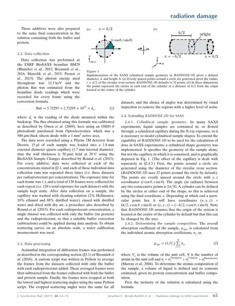
2.4.1. Cylindrical sample geometry. In many SAXS

experiments, liquid samples are contained in, or flowed

through, a cylindrical capillary during the X-ray exposure, so it

is necessary to model cylindrical sample shapes. To extend the

capability of RADDOSE-3D to be used for the calculation of

dose in SAXS experiments, a cylindrical shape geometry was

implemented. It specifies the geometry of the sample alone,

but not the capillary in which it is contained, and is graphically

depicted in Fig. 1. (The effect of the capillary is dealt with

separately in x2.4.3.) First, the points around a circle are

generated using the diameter of the circular cross section.

(RADDOSE-3D uses 32 points around the circle by default).

The points are evenly spaced around the circle with y; z

coordinates (r cos �; r sin �). The angle (in radians) between

any two consecutive points is 2�=32. A cylinder can be defined

by the circles at either end of the shape, so this is achieved

using the final coordinate x. Depending at which end a parti-

cular point lies, it will have coordinates (x; y; z) =

(h=2; r cos �; r sin �) or (x; y; z) = (�h=2; r cos �; r sin �). Note

that RADDOSE-3D assumes that the origin of the system is

located at the centre of the cylinder by default but that this can

be changed by the user.

2.4.2. Determining the sample composition. The overall

absorption coefficient of the sample, �abs, is calculated from

the individual atomic absorption coefficients, �j, as

�abs ¼ 1=Vcð ÞPN

j¼ 1

�j; ð2Þ

where Vc is the volume of the unit cell, N is the number of

atoms in the unit cell and �j = �Thompsonj + �Compton

j + �Photoelectricj

(Murray et al., 2004). To determine the atomic composition of

the sample, a volume of liquid is defined and its contents

estimated, given its protein concentration and buffer compo-

sition.

First the molarity of the solution is calculated using the

formula

radiation damage

J. Synchrotron Rad. (2017). 24, 63–72 Jonathan C. Brooks-Bartlett et al. � Radiation damage in SAXS experiments 65

Figure 1Implementation of the SAXS cylindrical sample geometry in RADDOSE-3D given a defineddiameter, d, and height, h. (a) Evenly spaced points around a circle are generated given the radius,r ¼ d=2, of the circular cross section. RADDOSE-3D defaults to 32 points. (b) In three dimensionsthe points represent the circles at each end of the cylinder at a distance of h=2 from the originlocated at the centre of the cylinder.

Molarity ðmol L�1Þ ¼

sample concentration ðg L�1Þ

molecular mass ðg mol�1Þ: ð3Þ

The sample concentration is provided in units of grams per

litre (� mg ml�1). The molecular mass of the molecule is

calculated from other parameters provided. If the sequence

file is given for the protein (the sample can also contain DNA

and RNA), then the molecular mass can be determined by

summing the molecular mass of each residue in the file.

Otherwise, an average molecular weight is used for each

residue (110.0 Da for protein residues, 339.5 Da for RNA

nucleotides and 327.0 Da for DNA nucleotides).

The number of molecules in the volume can then be

calculated by multiplying the molarity, volume and Avoga-

dro’s number (N = 6.022 � 1023 mol�1), and the result is then

rounded to the nearest integer.

2.4.3. Beam attenuation due to the capillary. In a typical

MX experiment at 100 K, a crystal is exposed directly to the

X-ray beam. In contrast, samples from SAXS experiments are

held inside a quartz capillary. Thus the X-ray flux is attenuated

due to the capillary, and account must be taken of this effect

before calculating the dose absorbed by the sample. The

transmission fraction of an X-ray beam due to a material with

mass thickness x and density � is given by

I=I0 ¼ exp�� �=�ð Þx

�; ð4Þ

where I is the emergent intensity of the beam after penetrating

the material, I0 is the incident intensity and �=� is defined as

the mass attenuation coefficient (Hubbell & Seltzer, 1995).

The mass thickness, x, is defined as the mass per unit area and

is given by x = �t where t is the thickness of the material. The

attenuation fraction caused by the capillary can hence be

calculated as 1� I=I0 .

The mass attenuation coefficients for each element are

tabulated in the National Institute of Standards and Tech-

nology (NIST) tables. For mixtures, the total attenuation

coefficient is given by

�=� ¼P

i

wið�=�Þi; ð5Þ

where wi and �=�ð Þi are the fraction by weight and the mass

attenuation coefficient of the ith atomic constituent, respec-

tively.

2.5. Dose calculation

Doses were calculated using RADDOSE-3D (Zeldin et al.,

2013a) and all doses referred to here are diffraction weighted

dose (DWD) values (Zeldin et al., 2013b). The flux was

calculated for each frame because the diode readings

continuously changed between frames due to the decay of the

electron current in the storage ring (see Fig. S1 of the

supporting information). However, the overall change in

diode current was only 0.54% during the course of a single

run. Despite the small percentage change, this effect was still

taken into account in the analysis.

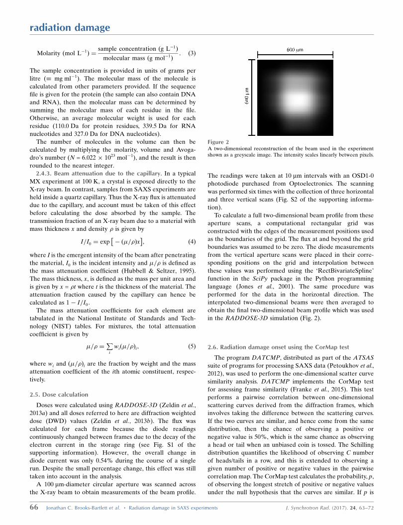
A 100 mm-diameter circular aperture was scanned across

the X-ray beam to obtain measurements of the beam profile.

The readings were taken at 10 mm intervals with an OSD1-0

photodiode purchased from Optoelectronics. The scanning

was performed six times with the collection of three horizontal

and three vertical scans (Fig. S2 of the supporting informa-

tion).

To calculate a full two-dimensional beam profile from these

aperture scans, a computational rectangular grid was

constructed with the edges of the measurement positions used

as the boundaries of the grid. The flux at and beyond the grid

boundaries was assumed to be zero. The diode measurements

from the vertical aperture scans were placed in their corre-

sponding positions on the grid and interpolation between

these values was performed using the ‘RectBivariateSpline’

function in the SciPy package in the Python programming

language (Jones et al., 2001). The same procedure was

performed for the data in the horizontal direction. The

interpolated two-dimensional beams were then averaged to

obtain the final two-dimensional beam profile which was used

in the RADDOSE-3D simulation (Fig. 2).

2.6. Radiation damage onset using the CorMap test

The program DATCMP, distributed as part of the ATSAS

suite of programs for processing SAXS data (Petoukhov et al.,

2012), was used to perform the one-dimensional scatter curve

similarity analysis. DATCMP implements the CorMap test

for assessing frame similarity (Franke et al., 2015). This test

performs a pairwise correlation between one-dimensional

scattering curves derived from the diffraction frames, which

involves taking the difference between the scattering curves.

If the two curves are similar, and hence come from the same

distribution, then the chance of observing a positive or

negative value is 50%, which is the same chance as observing

a head or tail when an unbiased coin is tossed. The Schilling

distribution quantifies the likelihood of observing C number

of heads/tails in a row, and this is extended to observing a

given number of positive or negative values in the pairwise

correlation map. The CorMap test calculates the probability, p,

of observing the longest stretch of positive or negative values

under the null hypothesis that the curves are similar. If p is

radiation damage

66 Jonathan C. Brooks-Bartlett et al. � Radiation damage in SAXS experiments J. Synchrotron Rad. (2017). 24, 63–72

Figure 2A two-dimensional reconstruction of the beam used in the experimentshown as a greyscale image. The intensity scales linearly between pixels.

above a given significance threshold, then the frames can be

considered similar.

For the purposes of the current investigation, the first three

frames of each experiment were compared in a pairwise

manner using the CorMap test to ensure that they were similar

(p value > 0.01). Then all subsequent frames were compared

with frame 1. Radiation damage was assumed to have become

significant at the point when three consecutive frames (in

order to exclude outliers, for example bubbles or particles,

passing through the beam) were found to be dissimilar as

determined by the CorMap test at the p = 0.01 significance

level. The dose absorbed in the sample for the first of the three

consecutive dissimilar frames was then denoted the threshold

dose, DThresh.

2.7. Signal reduction

As well as providing protection from radiation damage,

the addition of a radioprotectant compound to the sample

decreases the scattered intensity signal that constitutes the

experimental data.

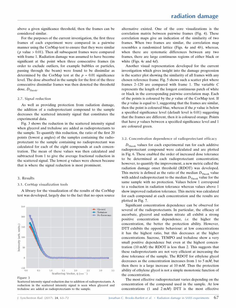
Fig. 3 shows the reduction in the scattered intensity signal

when glycerol and trehalose are added as radioprotectants to

the sample. To quantify this reduction, the ratio of the first 20

points (lowest q angles) of the samples containing the radio-

protectant to the sample containing no radioprotectant was

calculated for each of the eight compounds at each concen-

tration. The mean of these values was then calculated and

subtracted from 1 to give the average fractional reduction in

the scattered signal. The lowest q values were chosen because

that is where the signal reduction is most prominent.

3. Results

3.1. CorMap visualization tools

A library for the visualization of the results of the CorMap

test was developed, largely due to the fact that no open source

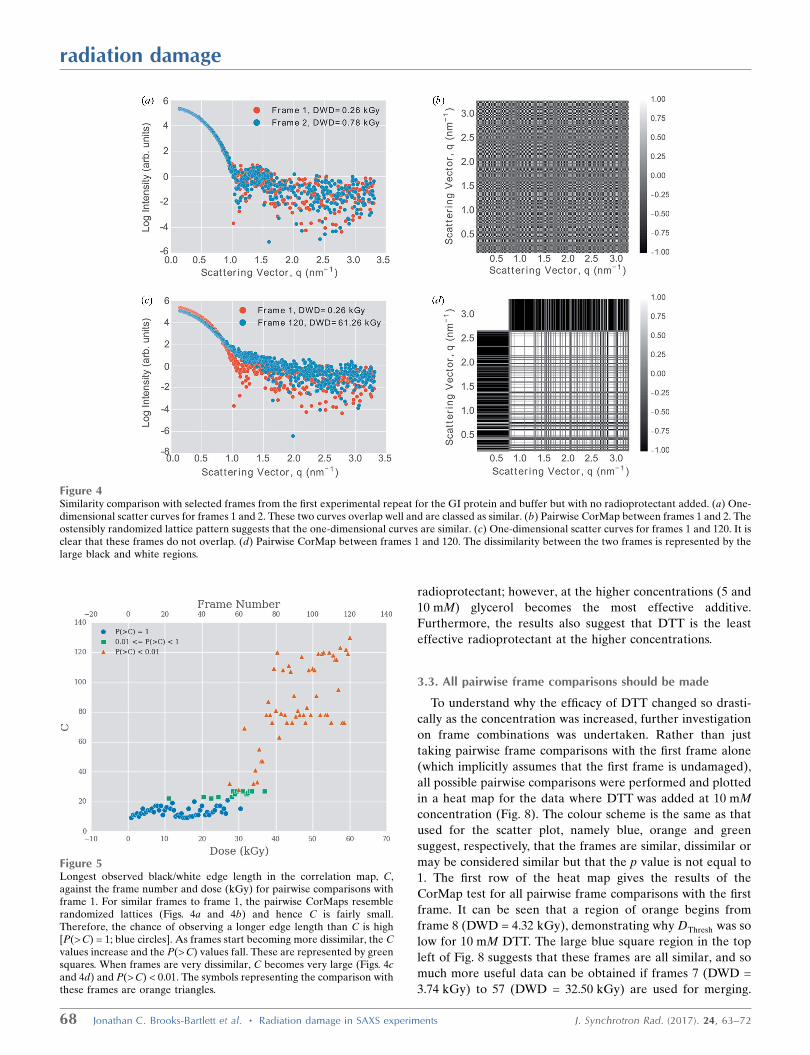
alternative existed. One of the core visualizations is the

correlation matrix between pairwise frames (Fig. 4). These

correlation maps give an indication of the similarity of two

frames. When two frames are similar, the correlation map

resembles a randomized lattice (Figs. 4a and 4b), whereas,

when there are systematic differences between any two

frames, there are large continuous regions of either black or

white (Figs. 4c and 4d).

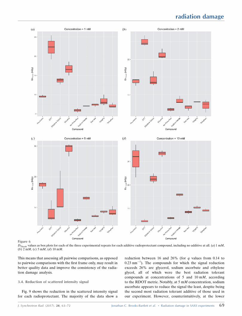
Another visual representation developed for the current

investigation which gives insight into the damage progression

is the scatter plot showing the similarity of all frames with any

chosen reference frame. Fig. 5 shows such a scatter plot where

frames 2–120 are compared with frame 1. The variable C

represents the length of the longest continuous patch of white

or black in the corresponding pairwise correlation map. Each

of the points is coloured by the p value of the CorMap test. If

the p value is equal to 1, suggesting that the frames are similar,

then the point is coloured blue, whereas if the p value is below

a specified significance level (default level is 0.01) suggesting

that the frames are different, then it is coloured orange. Points

that have p values between a specified significance level and 1

are coloured green.

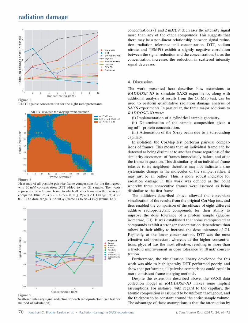
3.2. Concentration dependence of radioprotectant efficacy

DThresh values for each experimental run for each additive

radioprotectant compound were calculated and are plotted

in Fig. 6. These enabled the order of increased dose tolerance

to be determined at each radioprotectant concentration;

however, to quantify the improvement, a new metric called the

radiation damage onset threshold (RDOT) was developed.

This metric is defined as the ratio of the median DThresh value

with added radioprotectant to the median DThresh value for the

same sample with no protection. Values below 1 correspond

to a reduction in radiation tolerance whereas values above 1

show improved radiation tolerance. This metric was calculated

for each compound at each concentration and the results are

plotted in Fig. 7.

Significant concentration dependence can be observed for

several of the radioprotectants. In particular, the efficacy of

ascorbate, glycerol and sodium nitrate all exhibit a strong

positive concentration dependence, i.e. the higher the

concentration, the better the protection ability. However,

DTT exhibits the opposite behaviour: at low concentrations

it has the highest ratio, but this decreases at the higher

concentrations. Sucrose, TEMPO and trehalose show a very

small positive dependence but even at the highest concen-

tration (10 mM) the RDOT is less than 2. This suggests that

these radioprotectants are not very efficient at increasing the

dose tolerance of the sample. The RDOT for ethylene glycol

decreases as the concentration increases from 1 to 5 mM, but

then there is a large increase at 10 mM. Thus the protection

ability of ethylene glycol is not a simple monotonic function of

the concentration.

The most effective radioprotectant varies depending on the

concentration of the compound used in the sample. At low

concentrations (1 and 2 mM) DTT is the most effective

radiation damage

J. Synchrotron Rad. (2017). 24, 63–72 Jonathan C. Brooks-Bartlett et al. � Radiation damage in SAXS experiments 67

Figure 3Scattered intensity signal reduction due to addition of radioprotectants. Areduction in the scattered intensity signal is seen when glycerol andtrehalose are added as radioprotectants to the sample.

radioprotectant; however, at the higher concentrations (5 and

10 mM) glycerol becomes the most effective additive.

Furthermore, the results also suggest that DTT is the least

effective radioprotectant at the higher concentrations.

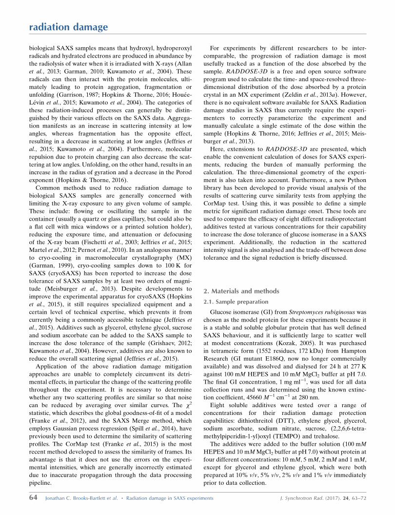
3.3. All pairwise frame comparisons should be made

To understand why the efficacy of DTT changed so drasti-

cally as the concentration was increased, further investigation

on frame combinations was undertaken. Rather than just

taking pairwise frame comparisons with the first frame alone

(which implicitly assumes that the first frame is undamaged),

all possible pairwise comparisons were performed and plotted

in a heat map for the data where DTT was added at 10 mM

concentration (Fig. 8). The colour scheme is the same as that

used for the scatter plot, namely blue, orange and green

suggest, respectively, that the frames are similar, dissimilar or

may be considered similar but that the p value is not equal to

1. The first row of the heat map gives the results of the

CorMap test for all pairwise frame comparisons with the first

frame. It can be seen that a region of orange begins from

frame 8 (DWD = 4.32 kGy), demonstrating why DThresh was so

low for 10 mM DTT. The large blue square region in the top

left of Fig. 8 suggests that these frames are all similar, and so

much more useful data can be obtained if frames 7 (DWD =

3.74 kGy) to 57 (DWD = 32.50 kGy) are used for merging.

radiation damage

68 Jonathan C. Brooks-Bartlett et al. � Radiation damage in SAXS experiments J. Synchrotron Rad. (2017). 24, 63–72

Figure 4Similarity comparison with selected frames from the first experimental repeat for the GI protein and buffer but with no radioprotectant added. (a) One-dimensional scatter curves for frames 1 and 2. These two curves overlap well and are classed as similar. (b) Pairwise CorMap between frames 1 and 2. Theostensibly randomized lattice pattern suggests that the one-dimensional curves are similar. (c) One-dimensional scatter curves for frames 1 and 120. It isclear that these frames do not overlap. (d) Pairwise CorMap between frames 1 and 120. The dissimilarity between the two frames is represented by thelarge black and white regions.

Figure 5Longest observed black/white edge length in the correlation map, C,against the frame number and dose (kGy) for pairwise comparisons withframe 1. For similar frames to frame 1, the pairwise CorMaps resemblerandomized lattices (Figs. 4a and 4b) and hence C is fairly small.Therefore, the chance of observing a longer edge length than C is high[P(> C) = 1; blue circles]. As frames start becoming more dissimilar, the Cvalues increase and the P(> C) values fall. These are represented by greensquares. When frames are very dissimilar, C becomes very large (Figs. 4cand 4d) and P(> C) < 0.01. The symbols representing the comparison withthese frames are orange triangles.

This means that assessing all pairwise comparisons, as opposed

to pairwise comparisons with the first frame only, may result in

better quality data and improve the consistency of the radia-

tion damage analysis.

3.4. Reduction of scattered intensity signal

Fig. 9 shows the reduction in the scattered intensity signal

for each radioprotectant. The majority of the data show a

reduction between 16 and 26% (for q values from 0.14 to

0.23 nm�1). The compounds for which the signal reduction

exceeds 26% are glycerol, sodium ascorbate and ethylene

glycol, all of which were the best radiation tolerant

compounds at concentrations of 5 and 10 mM, according

to the RDOT metric. Notably, at 5 mM concentration, sodium

ascorbate appears to reduce the signal the least, despite being

the second most radiation tolerant additive of those used in

our experiment. However, counterintuitively, at the lower

radiation damage

J. Synchrotron Rad. (2017). 24, 63–72 Jonathan C. Brooks-Bartlett et al. � Radiation damage in SAXS experiments 69

Figure 6DThresh values as box plots for each of the three experimental repeats for each additive radioprotectant compound, including no additive at all. (a) 1 mM,(b) 2 mM, (c) 5 mM, (d) 10 mM.

concentrations (1 and 2 mM), it decreases the intensity signal

more than any of the other compounds. This suggests that

there may be a non-linear relationship between signal reduc-

tion, radiation tolerance and concentration. DTT, sodium

nitrate and TEMPO exhibit a slightly negative correlation

between the signal reduction and the concentration, i.e. as the

concentration increases, the reduction in scattered intensity

signal decreases.

4. Discussion

The work presented here describes how extensions to

RADDOSE-3D to simulate SAXS experiments, along with

additional analysis of results from the CorMap test, can be

used to perform quantitative radiation damage analysis of

SAXS experiments. In particular, the three major additions to

RADDOSE-3D were:

(i) Implementation of a cylindrical sample geometry.

(ii) Determination of the sample composition given a

mg ml�1 protein concentration.

(iii) Attenuation of the X-ray beam due to a surrounding

capillary.

In isolation, the CorMap test performs pairwise compar-

isons of frames. This means that an individual frame can be

detected as being dissimilar to another frame regardless of the

similarity assessment of frames immediately before and after

the frame in question. This dissimilarity of an individual frame

relative to its neighbour therefore may not indicate a true

systematic change in the molecules of the sample; rather, it

may just be an outlier. Thus, a more robust indicator for

radiation damage in this work was defined as the point

whereby three consecutive frames were assessed as being

dissimilar to the first frame.

The additions described above allowed the convenient

visualization of the results from the original CorMap test, and

thus enabled the comparison of the efficacy of eight different

additive radioprotectant compounds for their ability to

improve the dose tolerance of a protein sample (glucose

isomerase, GI). It was established that some radioprotectant

compounds exhibit a stronger concentration dependence than

others in their ability to increase the dose tolerance of GI.

Explicitly, at the lower concentrations, DTT was the most

effective radioprotectant whereas, at the higher concentra-

tions, glycerol was the most effective, resulting in more than

a fivefold improvement in dose tolerance at 10 mM concen-

tration.

Furthermore, the visualization library developed for this

work was able to highlight why DTT performed poorly, and

show that performing all pairwise comparisons could result in

more consistent frame-merging methods.

Despite the extensions described above, the SAXS data

collection model in RADDOSE-3D makes some implicit

assumptions. For instance, with regard to the capillary, the

atomic composition is assumed to be uniform throughout, and

the thickness to be constant around the entire sample volume.

The advantage of these assumptions is that the attenuation by

radiation damage

70 Jonathan C. Brooks-Bartlett et al. � Radiation damage in SAXS experiments J. Synchrotron Rad. (2017). 24, 63–72

Figure 8Heat map of all possible pairwise frame comparisons for the first repeatwith 10 mM concentration DTT added to the GI sample. The y-axisrepresents the reference frame to which all other frames on the x-axis arecompared. Blue: P(> C) = 1. Green: 0.01 � P(> C) < 1. Orange: P(> C) <0.01. The dose range is 0.29 kGy (frame 1) to 68.74 kGy (frame 120).

Figure 7RDOT against concentration for the eight radioprotectants.

Figure 9Scattered intensity signal reduction for each radioprotectant (see text formethod of calculation).

the capillary only needs to be calculated once, regardless of

any movement or rotation of the capillary. This is valid for

a cylindrical capillary since the thickness penetrated by the

X-ray beam is the same regardless of any rotations or trans-

lations.

Additionally, the sample itself is assumed to be static,

moving as a rigid body when rotated or translated, and also

to be completely filling the capillary. This greatly reduces the

computational cost when compared with the possibility of

modelling more realistic fluid dynamics. The assumption that

the capillary volume is completely filled is generally valid since

this is usually the case during an experiment. The static

assumption, on the other hand, is not always appropriate,

especially when the sample is flowed through the capillary.

Hopkins & Thorne (2016) calculated that for typical experi-

mental parameters the velocity profile is expected to exhibit

the quadratic Poiseuille flow profile, which arises from the

axial symmetry and no-slip boundary assumptions (the velo-

city at the centre of the tube moves the fastest while the

velocity at the boundary is equal to zero provided the capillary

is also stationary). Hopkins & Thorne also calculated that the

residence times of the sample in the beam were too short for

any appreciable radial diffusive mixing, so that the flow profile

results in radius-dependent residence times in the X-ray beam.

Therefore, the static assumption made in RADDOSE-3D will

give misleading dose values if calculated for experiments

where the sample is flowed through the beam position.

Diffusive turnover is another phenomenon that will affect

the dose calculation. Molecules have the ability to diffuse into

and out of the illuminated volume, with the additional

complexity that a non-uniform beam profile will cause

differential diffusion across the beam due to higher sample

heating at the peak of the beam profile. In the current work,

no account was taken for molecular diffusion. However, beam

sizes in SAXS experiments are typically quite large and

exposure times are not long enough for the diffusive turnover

to cause a significant effect. For example, Jeffries et al. (2015)

used a 500 mm � 250 mm sized beam with a maximum expo-

sure time of 141 s per sample while irradiating at 283 K

(Jeffries et al., 2015).

An important consideration regarding the concentration

dependence of the efficacy of the additives is that they can

alter the preferred environments of the sample. For example,

it is known that DTT reduces disulfide bonds and undergoes

oxidation. Glycerol at higher concentrations, on the other

hand, is known to increase the noise and hence reduce the

observable signal obtained from the sample (Jeffries et al.,

2015). In our study the reduction in the scattered intensity

signal was examined for the different radioprotectants.

Generally, the best performing radioprotectants, in terms of

increasing the radiation tolerance of the sample, also reduced

the scattered signal most. However, this order is not neces-

sarily consistent, which suggests that the relationship is likely

to be non-linear. Therefore, striking the optimal balance

between increasing radiation tolerance and the level of signal

reduction will still require some level of experience and input

from the experimenter.

The definition of the signal reduction used in this study only

considered the differences of the scattered intensity curve at

the lowest q values where the difference was most prominent.

However, the shape of the one-dimensional scattering curve

can vary dramatically for different protein samples. Therefore,

a metric for assessing the reduction that faithfully accounts for

the difference across the entire q range may be more desirable.

Another important factor to consider is that the efficacy of

radioprotectants may alter for different protein samples. This

will likely be due to the various interaction processes that will

occur for different macromolecules. For example, radio-

protectants that performed best in this study could be involved

in the prevention of the GI tetramer oligomerization break-

down. This process may not be as important for other samples,

and hence the order of efficacy found in this study may not be

applicable to a different sample.

During the data processing stage, the data were cropped by

visual inspection to remove noisy sections. This is a subjective

choice and therefore reduces the reproducibility of this work.

To overcome this problem, quantitative criteria could be

applied to find the optimum cut-off values for the data.

Investigation of these possible criteria should be considered

for further investigation of this method.

The DThresh values in our study range between 2.37 and

51.24 kGy. These differ significantly from the various

threshold values in other types of diffraction experiments:

room-temperature MX �150–500 kGy (Roedig et al., 2015;

Southworth-Davies et al., 2007), cryo-crystallography

�30 MGy (Owen et al., 2006) and cryo-SAXS >3.7 MGy

for mL samples and between 100–300 kGy for nL samples

(Meisburger et al., 2013). These differences are likely to be

attributable to the differences in the experimental factors, e.g.

temperature, sample type etc. However, there is still significant

variation in the critical doses calculated for other room-

temperature SAXS experiments [�400 Gy (Kuwamoto et al.,

2004) and 284–7700 Gy (Jeffries et al.)] when compared with

the DThresh values calculated in our study. Some of the varia-

tion can be attributed to the different protein samples and

concentrations used in the experiments for the studies.

However, the most likely cause of the apparent discrepancy is

the various definitions of the critical dose. Hopkins & Thorne

(2016) show that applying the critical dose definition from

Jeffries et al. (2015) to their own GI data results in a critical

dose of �66000 kGy, whereas the range in the Jeffries et al.

(2015) study for GI was 5964–7056 Gy. Furthermore, they also

state that ‘the molecular weight shows a significant (13%)

change after just �75 kGy’. Hence the critical dose value is

highly dependent on the definition chosen to calculate it.

Additionally, differences can also be expected due to the fact

that the critical dose estimates from the previous studies are

based upon (pseudo) radius of gyration values, whereas in our

study the DThresh values are determined by analysis of frame

similarity.

Although these issues should be taken into account for any

given experiment to ensure optimum and successful data

collection, the ability to predict the dose expected in a

BioSAXS experiment and to rationally choose a suitable

radiation damage

J. Synchrotron Rad. (2017). 24, 63–72 Jonathan C. Brooks-Bartlett et al. � Radiation damage in SAXS experiments 71

additive to improve the starting conditions offers considerable

benefits for data quality and efficiency of BioSAXS experi-

ments. The methods and tools presented in this paper can be

used in a complementary manner to other metrics created for

assessing the quality of SAXS data (Grant et al., 2015;

Hopkins & Thorne, 2016).

The CorMap analysis visualization source code is freely

available on Github: https://github.com/GarmanGroup/

CorMapAnalysis.

Acknowledgements

We thank the ESRF for beam time under the auspices of the

Radiation Damage BAG and the staff of beamline BM29,

Martha Brennich and Petra Pernot, for their support. We

gratefully acknowledge the UK Engineering and Physical

Sciences Research Council for studentship funding in the

Systems Biology Programme of the University of Oxford

Doctoral Training Centre (JBB and CSB, grant number EP/

G03706X/1), and studentship funding from the Wellcome

Trust (HMG, studentship number 075491/04). We also thank

the referees for their insightful comments.

References

Allan, E. G., Kander, M. C., Carmichael, I. & Garman, E. F. (2013).J. Synchrotron Rad. 20, 23–36.

Bizien, T., Durand, D., Roblina, P., Thureau, A., Vachette, P. & Perez,J. (2016). Protein Pept. Lett. 23, 217–231.

Blanchet, C. E., Spilotros, A., Schwemmer, F., Graewert, M. A.,Kikhney, A., Jeffries, C. M., Franke, D., Mark, D., Zengerle, R.,Cipriani, F., Fiedler, S., Roessle, M. & Svergun, D. I. (2015). J. Appl.Cryst. 48, 431–443.

Brennich, M. E., Kieffer, J., Bonamis, G., De Maria Antolinos, A.,Hutin, S., Pernot, P. & Round, A. (2016). J. Appl. Cryst. 49, 203–212.

Fischetti, R. F., Rodi, D. J., Mirza, A., Irving, T. C., Kondrashkina, E.& Makowski, L. (2003). J. Synchrotron Rad. 10, 398–404.

Franke, D., Jeffries, C. M. & Svergun, D. I. (2015). Nat. Methods, 12,419–422.

Franke, D., Kikhney, A. G. & Svergun, D. I. (2012). Nucl. Instrum.Methods Phys. Res. A, 689, 52–59.

Garman, E. (1999). Acta Cryst. D55, 1641–1653.Garman, E. F. (2010). Acta Cryst. D66, 339–351.Garrison, W. M. (1987). Chem. Rev. 87, 381–398.Graewert, M. A. & Svergun, D. I. (2013). Curr. Opin. Struct. Biol. 23,

748–754.Grant, T. D., Luft, J. R., Carter, L. G., Matsui, T., Weiss, T. M., Martel,

A. & Snell, E. H. (2015). Acta Cryst. D71, 45–56.Grishaev, A. (2012). Curr. Protoc. Protein. Sci. 70, 17.14.1–17.14.18.

Hopkins, J. B., Katz, A. M., Meisburger, S. P., Warkentin, M. A.,Thorne, R. E. & Pollack, L. (2015). J. Appl. Cryst. 48, 227–237.

Hopkins, J. B. & Thorne, R. E. (2016). J. Appl. Cryst. 49, 880–890.Houee-Levin, C., Bobrowski, K., Horakova, L., Karademir, B.,

Schoneich, C., Davies, M. J. & Spickett, C. M. (2015). Free Radic.Res. 49, 347–373.

Hubbell, J. & Seltzer, S. (1995). Report NISTIR 5632. NationalInstitute of Standards and Technology, Gaithersburg, MD, USA.

Jeffries, C. M., Graewert, M. A., Svergun, D. I. & Blanchet, C. E.(2015). J. Synchrotron Rad. 22, 273–279.

Jones, E., Oliphant, T., Peterson, P. & others (2001). SciPy: Opensource scientific tools for Python, http://www.scipy.org/.

Kozak, M. (2005). J. Appl. Cryst. 38, 555–558.Kuwamoto, S., Akiyama, S. & Fujisawa, T. (2004). J. Synchrotron Rad.

11, 462–468.Martel, A., Liu, P., Weiss, T. M., Niebuhr, M. & Tsuruta, H. (2012).

J. Synchrotron Rad. 19, 431–434.Materlik, G., Rayment, T. & Stuart, D. I. (2015). Philos. Trans. R. Soc.

A, 373, 20130161.Meisburger, S. P., Warkentin, M., Chen, H., Hopkins, J. B., Gillilan,

R. E., Pollack, L. & Thorne, R. E. (2013). Biophys. J. 104, 227–236.

Murray, J. W., Garman, E. F. & Ravelli, R. B. G. (2004). J. Appl. Cryst.37, 513–522.

Owen, R. L., Holton, J. M., Schulze-Briese, C. & Garman, E. F.(2009). J. Synchrotron Rad. 16, 143–151.

Owen, R. L., Rudino-Pinera, E. & Garman, E. F. (2006). Proc. NatlAcad. Sci. 103, 4912–4917.

Pernot, P., Round, A., Barrett, R., De Maria Antolinos, A., Gobbo,A., Gordon, E., Huet, J., Kieffer, J., Lentini, M., Mattenet, M.,Morawe, C., Mueller-Dieckmann, C., Ohlsson, S., Schmid, W.,Surr, J., Theveneau, P., Zerrad, L. & McSweeney, S. (2013).J. Synchrotron Rad. 20, 660–664.

Pernot, P., Theveneau, P., Giraud, T., Fernandes, R. N., Nurizzo, D.,Spruce, D., Surr, J., McSweeney, S., Round, A., Felisaz, F.,Foedinger, L., Gobbo, A., Huet, J., Villard, C. & Cipriani, F.(2010). J. Phys. Conf. Ser. 247, 012009.

Petoukhov, M. V., Franke, D., Shkumatov, A. V., Tria, G., Kikhney,A. G., Gajda, M., Gorba, C., Mertens, H. D. T., Konarev, P. V. &Svergun, D. I. (2012). J. Appl. Cryst. 45, 342–350.

Roedig, P., Vartiainen, I., Duman, R., Panneerselvam, S., Stube, N.,Lorbeer, O., Warmer, M., Sutton, G., Stuart, D. I., Weckert, E.,David, C., Wagner, A. & Meents, A. (2015). Sci. Rep. 5, 10451.

Round, A., Felisaz, F., Fodinger, L., Gobbo, A., Huet, J., Villard, C.,Blanchet, C. E., Pernot, P., McSweeney, S., Roessle, M., Svergun,D. I. & Cipriani, F. (2015). Acta Cryst. D71, 67–75.

Southworth-Davies, R. J., Medina, M. A., Carmichael, I. & Garman,E. F. (2007). Structure, 15, 1531–1541.

Spill, Y. G., Kim, S. J., Schneidman-Duhovny, D., Russel, D., Webb, B.,Sali, A. & Nilges, M. (2014). J. Synchrotron Rad. 21, 203–208.

Zeldin, O. B., Brockhauser, S., Bremridge, J., Holton, J. M. & Garman,E. F. (2013b). Proc. Natl Acad. Sci. 110, 20551–20556.

Zeldin, O. B., Gerstel, M. & Garman, E. F. (2013a). J. Appl. Cryst. 46,1225–1230.

radiation damage

72 Jonathan C. Brooks-Bartlett et al. � Radiation damage in SAXS experiments J. Synchrotron Rad. (2017). 24, 63–72