Page 1
Devices for measuring soil moisture:
Selecting sensors for use with the SoilWaterApp
Brett Robinson1
1 National Centre for Engineering in Agriculture, University of Southern Queensland, PO Box
555 Toowoomba, QLD 4350
Objectives of the review
1. To consider the economics of investing in modelling and monitoring soil water,
2. To outline the main limitations different types of soil water sensors, and
3. To choose two or three types of sensor for field use, connection to iPhones and for
integration with the Soilwaterapp.
Page 3
Summary
Besides the difficulty of interpreting soil moisture data, the main limitations to deploying
soil moisture sensors in dryland grain production are likely to be: (i) complexity, (ii) cost, (iii)
uncertainty, (iv) safety regulations, (v) installation problems and (vi) operating problems.
Which methods and sensors are unsuitable? Safety regulations preclude the use of neutron
probes, which are otherwise excellent sensors. Watermark sensors and tensiometers do not
work in dry soils, and can be excluded from consideration. Labour costs preclude methods
that require coring for samples (hand feel and psychrometers). Down-tube capacitance
sensors (C-probes and others) have a small volume of measurement that is easily affected
by artefacts associated with the tube, especially in shrink-swell soils. Time-domain
reflectometry (TDR) is expensive and unsuitable for shrink-swell soils due to poor soil
contact. Thermal conductivity and spectrometric methods lack commercial development
that might validate their accuracy and reliability. Penetrometers (push probes) are very
cheap and highly reliable, but are rarely calibrated and have low accuracy without
calibration.
Which methods and sensors are suitable? High frequency, buried capacitance sensors
(Sentek, Decagon and Vegetronix) are the best of the high-frequency capacitance probes.
Unfortunately, the cheapest (Vegetronix) has a small volume of measurement. Gypsum
blocks are cheap, but require conversion of soil water tension (kPa) measurements to water
content (%). EMI is accurate and measures hundreds of litres of undisturbed soil. However,
EMI sensors are expensive (but can me made cheaply). Spectrometric methods require
research and commercialisation. Push probes are suitable given quality calibration, but are
affected by salinity and compaction.
The following sensors should be tested in dryland grain production.
1. The Decagon HS10 sensor is a very high frequency (VHF) capacitance sensor. They
are accurate, reasonably cheap ($120-$150 each), may be read manually or logged,
and the volume of measurement is useful at approximately 1 litre.
2. The Vegetronics sensor is also a VHF capacitance sensor. It costs less than the
Decagon HS10 (at around $40) but unfortunately has a much smaller volume of
measurement.
3. Gypsum blocks are cheap ultra-low frequency (ULF) capacitance sensors ($25 each),
and may be manually metered or logged. They require a calibration curve that varies
with soil texture.
4. Penetrometers/‘push probes’ can be made more accurate with calibration and
careful use, adding to their already widespread use as a low-resolution sensor.
Page 4
Review of methods and sensors
Measuring soil water tension (SWT)
Hand feel and soil appearance
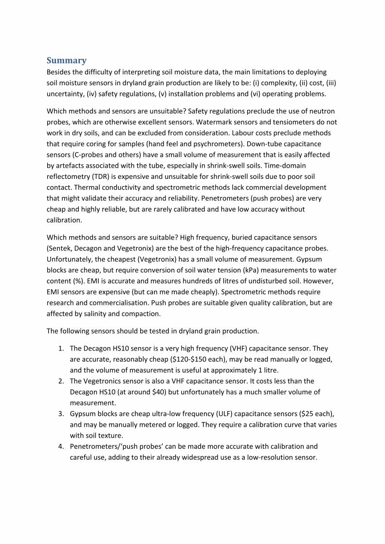
Clearly, this is used by farmers, consultants and scientists alike as a simple approximation of soil
wetness and moisture content. Most people have an intuitive understanding of soil wetness. The
relevance of this method is increased by standardised observations that can be categorised by
classes of soil texture to give tension and water content (see Figure 1).
The technique works for a variety of reasons:
• at low tension, pressure in the hand releases water from the soil,
• soil strength is highly correlated with moisture content,
• soil structure depends on moisture content (e.g. some clay soils lose structure when wet),
and
• clay is rigid when dry, and mouldable when moist, and is a lubricant when wet
Figure 1. The difference between a moist soil and a slightly drier soil is obvious.
http://www.jmmds.com/2011/04/spring-is-sprung%E2%80%94but-don%E2%80%99t-jump-the-gun/
Table 1 below is a guide to the characteristics of soils at different levels of wetness (USDA, 1998).
Photographs are very helpful. Table 1 also takes into account soil texture and shows estimates of
SWC (in imperial units of inches of water per foot of soil depth).
Pros:
• no electronic sensors
Cons:
• difficulty and cost of obtaining samples from the lower soil horizons
• medium accuracy
Assessment: Coring and hand feel are unsuitable for use in the project
Page 5
Table 1 Advice from the US Dept of Agriculture for estimating SWT from the hand feel and
appearance of soil. (SMD = Soil Moisture Deficit)
Page 6
Tensiometers
As suggested by the name, they measure the tension between soil water and the soil. A classic
tensiometer has a tube full of water at installation, and water is moved out of the tube by any
tension in the surrounding soil water, leaving a vacuum in the tube that is in equilibrium and
opposition to the soil water tension in the soil. Hi-tech tensioners use electronic pressure sensors
and do not need re-filling if the soil water tension empties the reservoir. A pressure gauge displays
the strength of the vacuum.
The tube is about 1 metre long and is capable of producing almost 1 bar of tension (100 kPa). This is
too little for dryland agriculture, where volumetrically there is approximately half of the available
PAWC ‘held’ at 1.5 to 15 bars.
Pros:
• long-established and accurate method
• low cost
• new types have electronic modules for continuous measurement
Cons:
• small range of tension measurement (0 to 1 bar)
• requires careful installation
Assessment: Tensiometers are unsuitable for measurements in dryland agriculture due to their
limited range of measurement (wet soils only)
Image courtesy of OreMax (http://www.ore-
max.com/?page=dont_drown_the_oxygen)
Figure 2
Page 7
Measuring the moisture content of soil air: Psychrometers
With respect to moisture availability, soil air is in equilibrium with soil water. Psychrometers
precisely measure the moisture content of soil air, and by calculation, the soil water potential. They
are widely used for atmospheric measurements, such as monitoring the effectiveness of air
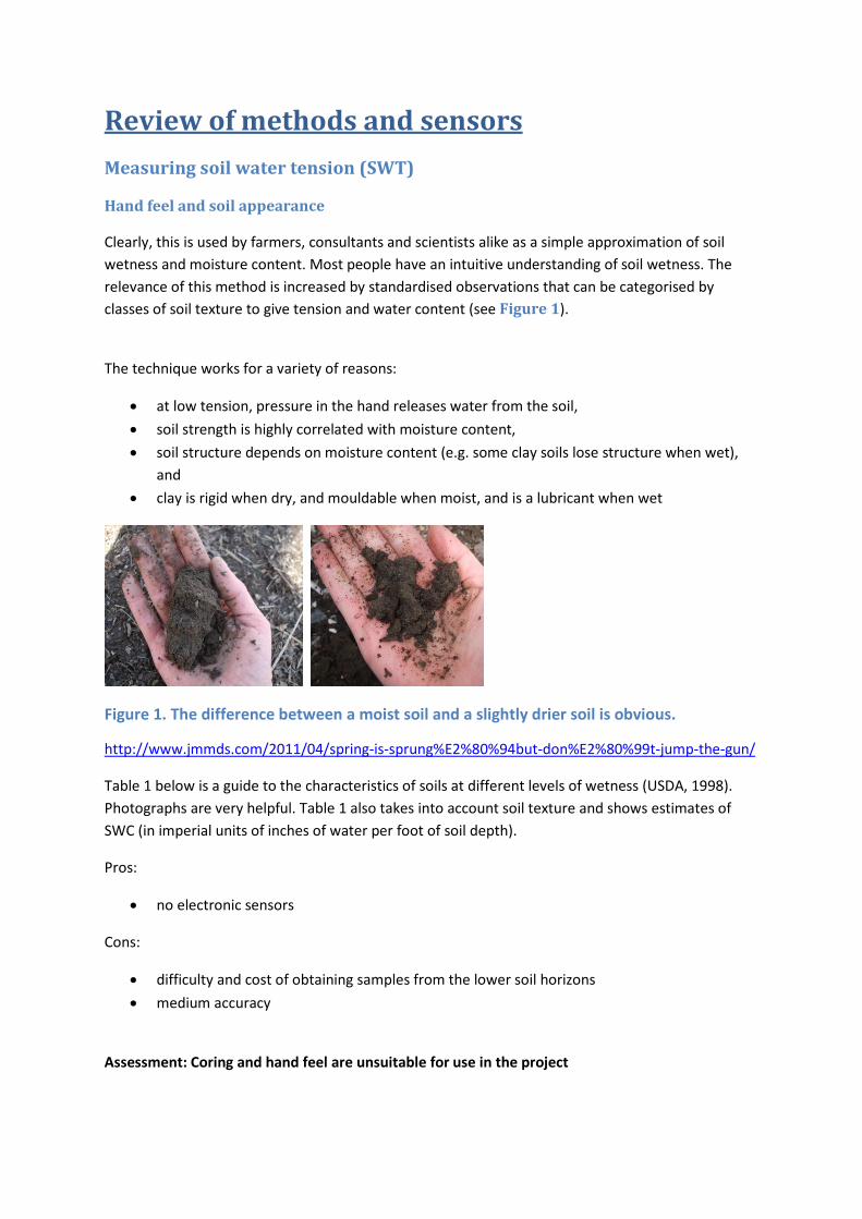
conditioning units and for calculating evaporation. The common apparatus for doing this is a rotating
or ‘sling’ psychrometer, shown below.
A rotating psychrometer, containing wet and dry bulb
thermometers. When swung in the air, the wet bulb temperature
is reduced to the dew point and the dry bulb measures the air
temperature. The handle contains a scale for calculating relative
humidity from the dry bulb temperature and the dry-wet
temperature difference.
Photo courtesy of http://www.plantfog.at/ZU_E/Zubehoer_E2.htm.
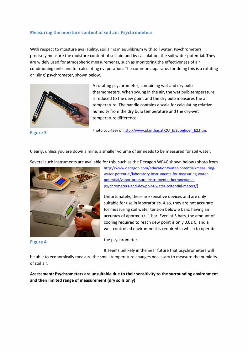
Clearly, unless you are down a mine, a smaller volume of air needs to be measured for soil water.
Several such instruments are available for this, such as the Decagon WP4C shown below (photo from
http://www.decagon.com/education/water-potential/measuring-
water-potential/laboratory-instruments-for-measuring-water-
potential/vapor-pressure-instruments-thermocouple-
psychrometers-and-dewpoint-water-potential-meters/).
Unfortunately, these are sensitive devices and are only
suitable for use in laboratories. Also, they are not accurate
for measuring soil water tension below 5 bars, having an
accuracy of approx. +/- 1 bar. Even at 5 bars, the amount of
cooling required to reach dew point is only 0.01 C, and a
well-controlled environment is required in which to operate
the psychrometer.
It seems unlikely in the near future that psychrometers will
be able to economically measure the small temperature changes necessary to measure the humidity
of soil air.
Assessment: Psychrometers are unsuitable due to their sensitivity to the surrounding environment
and their limited range of measurement (dry soils only)
Figure 3
Figure 4
Page 8
Thermal conductivity of the soil water in a porous block
Water is a moderately good conductor of heat, while air is a good insulator. Therefore, wet soils and
other porous materials become better conductors of heat as they become wetter. This is a precise
relationship and is almost unaffected by interference from soil salinity and other factors. Most of
these sensors work by heating the water in an area within a porous ceramic material (an insulator)
and detecting the rate of heating in another part of the material. Temperature rise per second (C/s)
is the usual measurement, taken from thermocouples in the ceramic. The time needed for a
measurement ranges from a few seconds to a minute.
Figure 5. A calibration curve between soil water content and soil thermal conductivity
(from Bristow et al. 2001).
Pros:
• simplicity
• accurate in moist to dry soils (0.1 to 20 bars of tension)
• comes with a calibration curve for SWT
• robust
Cons:
• expensive and sensitive equipment
• low accuracy in wet soils (0 to 0.1 bar)
• not widely used
• requires a programmed datalogger to coordinate the heating pulse and measurements
Assessment: thermal conductivity is potentially suitable for use in the project. The main
limitations are cost and lack of prior commercial application.
Page 9
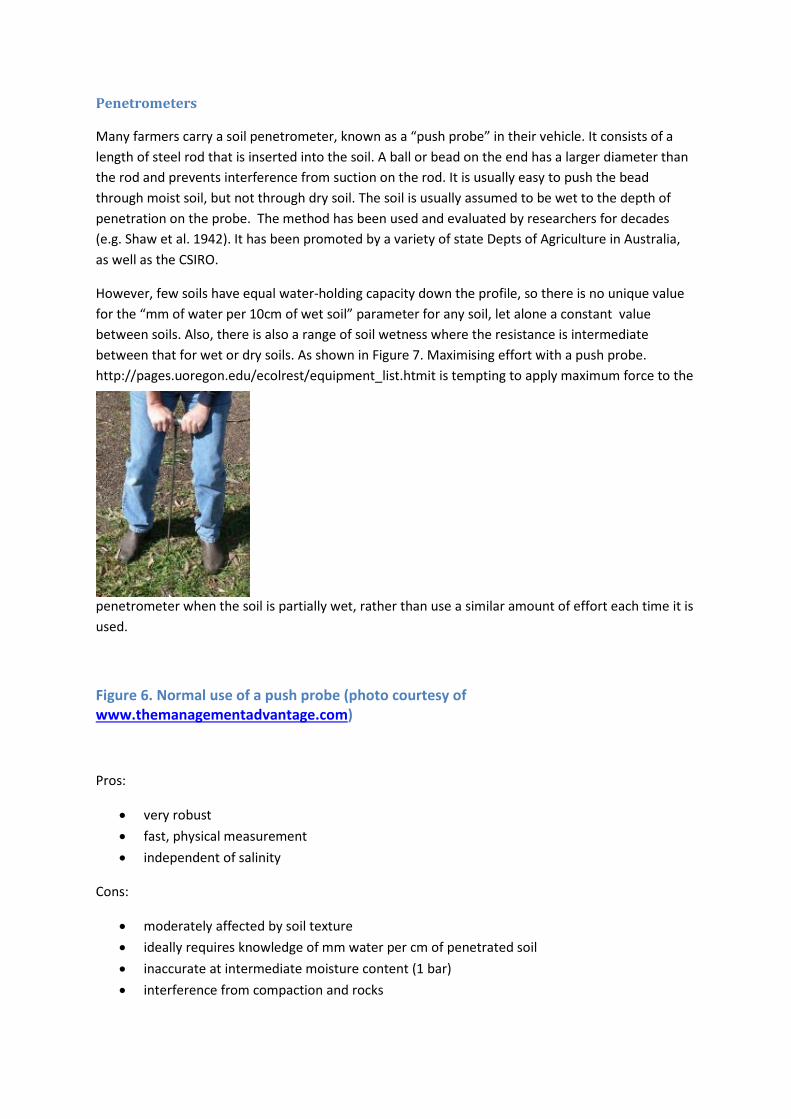
Penetrometers
Many farmers carry a soil penetrometer, known as a “push probe” in their vehicle. It consists of a
length of steel rod that is inserted into the soil. A ball or bead on the end has a larger diameter than
the rod and prevents interference from suction on the rod. It is usually easy to push the bead
through moist soil, but not through dry soil. The soil is usually assumed to be wet to the depth of
penetration on the probe. The method has been used and evaluated by researchers for decades
(e.g. Shaw et al. 1942). It has been promoted by a variety of state Depts of Agriculture in Australia,
as well as the CSIRO.
However, few soils have equal water-holding capacity down the profile, so there is no unique value
for the “mm of water per 10cm of wet soil” parameter for any soil, let alone a constant value
between soils. Also, there is also a range of soil wetness where the resistance is intermediate
between that for wet or dry soils. As shown in Figure 7. Maximising effort with a push probe.
http://pages.uoregon.edu/ecolrest/equipment_list.htmit is tempting to apply maximum force to the
penetrometer when the soil is partially wet, rather than use a similar amount of effort each time it is
used.
Figure 6. Normal use of a push probe (photo courtesy of
www.themanagementadvantage.com)
Pros:
• very robust
• fast, physical measurement
• independent of salinity
Cons:
• moderately affected by soil texture
• ideally requires knowledge of mm water per cm of penetrated soil
• inaccurate at intermediate moisture content (1 bar)
• interference from compaction and rocks
Page 10
Figure 7. Maximising effort with a push probe.
http://pages.uoregon.edu/ecolrest/equipment_list.htm
Assessment: push probes are potentially suitable for use in the project, but need better
calibration.
Page 11
Measuring soil water content (SWC)
Electromagnetic methods (capacitance, AC resistance, electromagnetic induction)
Background to the method
These sensors all measure the dielectric constant of soil. Water has a high volumetric dielectric
constant (80) compared to air (1), so soil water content is almost proportional the dielectric value.
The measurement is relatively simple, because dielectric materials respond to electro-magnetic
fields.
Water reacts strongly to electro-magnetic (EM) fields because it is a polar compound and the
molecules align with the field. Air is virtually non-polar and doesn’t react. Some minor soil
components, such as organic matter, are also dielectrics and have a small effect on the results.
Magnetic minerals may have an “anti-dielectric” effect on measurements because they have some
responses to EM that are the inverse of the effects of dielectrics.
Some of these sensors are called capacitance probes because dielectric compounds have electrical
storage capacity and are used to make the capacitors that are widely used in electronic circuits. An
easy way to measure the dielectric compounds in soil is to measure the associated soil capacitance,
using this relationship:
C = 1/(2.π.f.Z)
where C is capacitance (microFarads), and the other parameters are either known or easily
measured. Z is resistance (ohms), π ≈ 3.14, and f is frequency (kHz). The frequency (f) may be either
low (about 1 kHz for gypsum blocks) or high (about 100 MHz for capacitance probes) to avoid
interference that may occur at intermediate frequencies. The different sensors and methods are
reviewed separately below.
Figure 8. A schematic of a capacitor, including its
dielectric material (in orange). The polar molecules of a
dielectric are aligned by an external charge on one or
other of the plates. Via the dielectric, a charge +Q on
one plate induces a charge of –Q on the other, and vice
versa. An alternating charge on one plate induces an
inverse alternating charge on the other, thereby
conducting an alternating current in the absence of a
conductor (wrt to DC). (Image from
www.wikipedia.com)
Page 12
Gypsum blocks.
From http://www.dpi.vic.gov.au/agriculture/farming-management/soil-water/soil/ag0294-gypsum-
blocks-for-measuring-the-dryness-of-soil
“Gypsum blocks consist of two electrodes embedded in a block of gypsum…. Wires are joined onto
each electrode and extruded from the gypsum block to measure the resistance between the
electrodes. The resistance between the two electrodes varies with the water content in the gypsum
block, which will depend directly on the soil water tension. As the soil dries out water is extracted
from the gypsum block and the resistance between the electrodes increases. Conversely as the soil
wets, water is drawn back into the gypsum block and the resistance decreases.”
A gypsum block has a fine porous structure like many soils, and the gypsum is sparingly soluble,
providing a dilute salt solution that masks the effects of variable soil salinity. The dielectric value
(and capacitance) of the sensor change almost exclusively with change in the water content. Gypsum
blocks are variable from manufacturer to manufacturer and to a lesser extent from device to device,
but in general are well-suited to measuring the range of water content and tension of interest in
dryland agriculture. It is ironic that their main use has been in irrigated agriculture, as they have
least accuracy in wet soils, due to the low density (or absence) of large pores in the blocks.
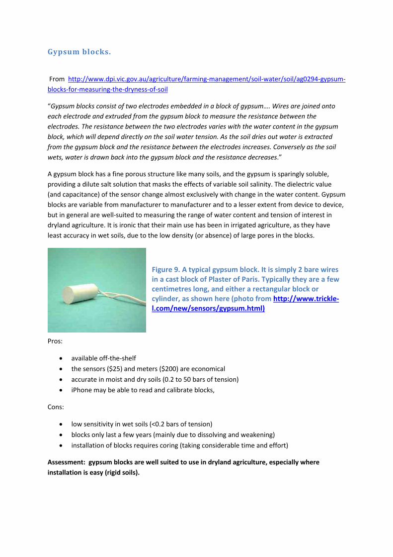
Figure 9. A typical gypsum block. It is simply 2 bare wires
in a cast block of Plaster of Paris. Typically they are a few
centimetres long, and either a rectangular block or
cylinder, as shown here (photo from http://www.trickle-
l.com/new/sensors/gypsum.html)
Pros:
• available off-the-shelf
• the sensors ($25) and meters ($200) are economical
• accurate in moist and dry soils (0.2 to 50 bars of tension)
• iPhone may be able to read and calibrate blocks,
Cons:
• low sensitivity in wet soils (<0.2 bars of tension)
• blocks only last a few years (mainly due to dissolving and weakening)
• installation of blocks requires coring (taking considerable time and effort)
Assessment: gypsum blocks are well suited to use in dryland agriculture, especially where
installation is easy (rigid soils).
Page 13
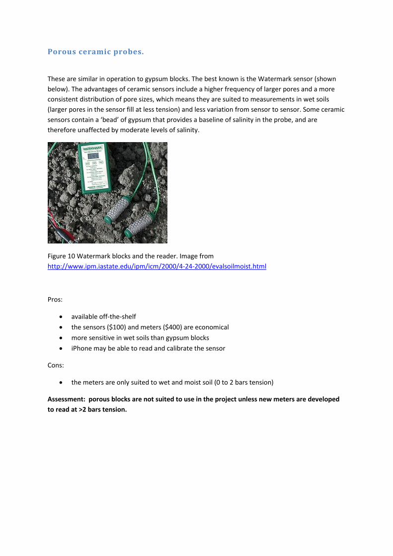
Porous ceramic probes.
These are similar in operation to gypsum blocks. The best known is the Watermark sensor (shown
below). The advantages of ceramic sensors include a higher frequency of larger pores and a more
consistent distribution of pore sizes, which means they are suited to measurements in wet soils
(larger pores in the sensor fill at less tension) and less variation from sensor to sensor. Some ceramic
sensors contain a ‘bead’ of gypsum that provides a baseline of salinity in the probe, and are
therefore unaffected by moderate levels of salinity.
Figure 10 Watermark blocks and the reader. Image from
http://www.ipm.iastate.edu/ipm/icm/2000/4-24-2000/evalsoilmoist.html
Pros:
• available off-the-shelf
• the sensors ($100) and meters ($400) are economical
• more sensitive in wet soils than gypsum blocks
• iPhone may be able to read and calibrate the sensor
Cons:
• the meters are only suited to wet and moist soil (0 to 2 bars tension)
Assessment: porous blocks are not suited to use in the project unless new meters are developed
to read at >2 bars tension.
Page 14
Time-Domain reflectometry (TDR).
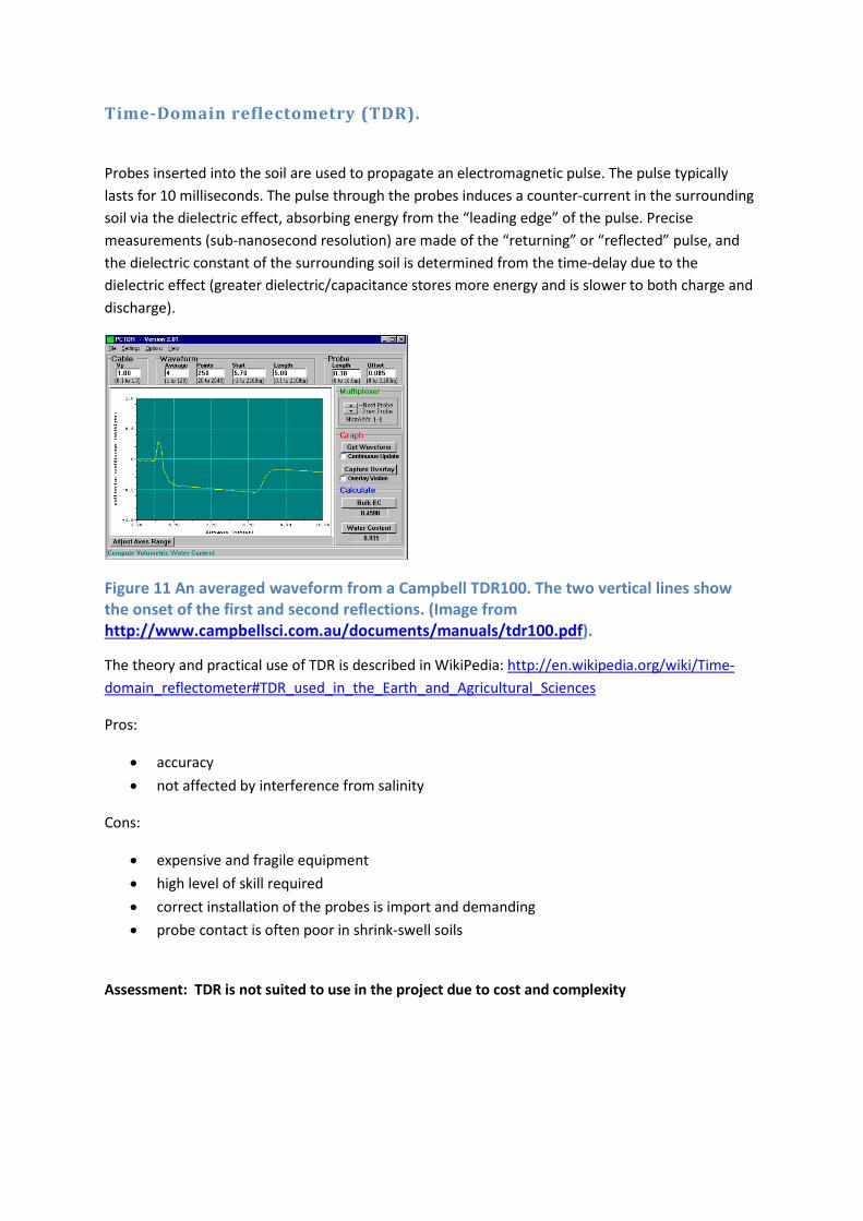
Probes inserted into the soil are used to propagate an electromagnetic pulse. The pulse typically
lasts for 10 milliseconds. The pulse through the probes induces a counter-current in the surrounding
soil via the dielectric effect, absorbing energy from the “leading edge” of the pulse. Precise
measurements (sub-nanosecond resolution) are made of the “returning” or “reflected” pulse, and
the dielectric constant of the surrounding soil is determined from the time-delay due to the
dielectric effect (greater dielectric/capacitance stores more energy and is slower to both charge and
discharge).
Figure 11 An averaged waveform from a Campbell TDR100. The two vertical lines show
the onset of the first and second reflections. (Image from
http://www.campbellsci.com.au/documents/manuals/tdr100.pdf).
The theory and practical use of TDR is described in WikiPedia: http://en.wikipedia.org/wiki/Time-
domain_reflectometer#TDR_used_in_the_Earth_and_Agricultural_Sciences
Pros:
• accuracy
• not affected by interference from salinity
Cons:
• expensive and fragile equipment
• high level of skill required
• correct installation of the probes is import and demanding
• probe contact is often poor in shrink-swell soils
Assessment: TDR is not suited to use in the project due to cost and complexity
Page 15
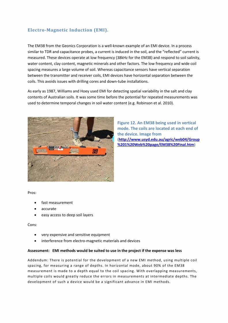
Electro-Magnetic Induction (EMI).
The EM38 from the Geonics Corporation is a well-known example of an EMI device. In a process
similar to TDR and capacitance probes, a current is induced in the soil, and the “reflected” current is
measured. These devices operate at low frequency (38kHz for the EM38) and respond to soil salinity,
water content, clay content, magnetic minerals and other factors. The low frequency and wide coil
spacing measures a large volume of soil. Whereas capacitance sensors have vertical separation
between the transmitter and receiver coils, EMI devices have horizontal separation between the
coils. This avoids issues with drilling cores and down-tube installations.
As early as 1987, Williams and Hoey used EMI for detecting spatial variability in the salt and clay
contents of Australian soils. It was some time before the potential for repeated measurements was
used to determine temporal changes in soil water content (e.g. Robinson et al. 2010).
Figure 12. An EM38 being used in vertical
mode. The coils are located at each end of
the device. Image from (http://www.usyd.edu.au/agric/web04/Group
%201%20Web%20page/EM38%20Final.htm)
Pros:
• fast measurement
• accurate
• easy access to deep soil layers
Cons:
• very expensive and sensitive equipment
• interference from electro-magnetic materials and devices
Assessment: EMI methods would be suited to use in the project if the expense was less
Addendum: There is potential for the development of a new EMI method, using multiple coil
spacing, for measuring a range of depths. In horizontal mode, about 90% of the EM38
measurement is made to a depth equal to the coil spacing. With overlapping measurements,
multiple coils would greatly reduce the errors in measurements at intermediate depths. The
development of such a device would be a significant advance in EMI methods.
Page 16
Non-contact capacitance sensors (high frequency ‘probes’).
Capacitance probes use a high-frequency current (approx. 100 MHz) and coils with close vertical
spacing. The sensors maybe be permanently located within PVC access tubes (C-probe) or placed in a
tube as needed (Gopher) or encapsulated and buried. It is usual for 3 or 4 depths to be measured by
6 or 8 coils. The measurements are typically logged at frequent intervals (sub-daily).
Figure 13. An EnviroScan probe, with multiple
sensors that are positioned down a PVC tube.
Image from
(http://web.fi.ibimet.cnr.it/idri/s_enviroscan.htm)
An excellent summary of the use of these sensors in agriculture is available here:
http://www.dpi.nsw.gov.au/data/assets/pdf_file/0009/165078/capacitance-probes.pdf
Frequency domain sensors, including those known as capacitance probes, are described in these
articles: http://en.wikipedia.org/wiki/Frequency_domain_sensor
http://en.wikipedia.org/wiki/Capacitance_probe
Pros:
• accurate
• easy access to deep soil layers
Cons:
• expensive, sensitive equipment
• requires expert installation
• effects of the access tube
Assessment: Non-contact capacitance sensors are more expensive and complex than other
capacitance methods, and the results may be affected by the presence of the access tube
Page 17
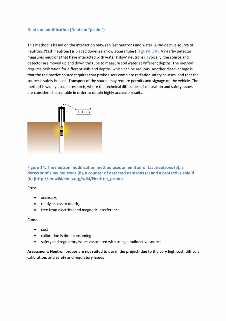
Neutron modification (Neutron “probe”)
This method is based on the interaction between ‘ast neutrons and water. A radioactive source of
neutrons (‘fast’ neutrons) is placed down a narrow access tube (Figure 14). A nearby detector
measures neutrons that have interacted with water (‘slow’ neutrons). Typically, the source and
detector are moved up and down the tube to measure soil water at different depths. The method
requires calibration for different soils and depths, which can be arduous. Another disadvantage is
that the radioactive source requires that probe users complete radiation safety courses, and that the
source is safely housed. Transport of the source may require permits and signage on the vehicle. The
method is widely used in research, where the technical difficulties of calibration and safety issues
are considered acceptable in order to obtain highly accurate results.
Figure 14. The neutron modification method uses an emitter of fast neutrons (e), a
detector of slow neutrons (d), a counter of detected neutrons (c) and a protective shield
(b) (http://en.wikipedia.org/wiki/Neutron_probe)
Pros:
• accuracy,
• ready access to depth,
• free from electrical and magnetic interference
Cons:
• cost
• calibration is time-consuming
• safety and regulatory issues associated with using a radioactive source
Assessment: Neutron probes are not suited to use in the project, due to the very high cost, difficult
calibration, and safety and regulatory issues
Page 18
Spectrometric methods (infra-red, near infra-red, visible, UV)
Wet soil is darker than dry soil due to the absorption of visible radiation by water in soil, hinting at
the ease with which spectrometric methods might measure soil water content. Similarly, water has
characteristic absorption of electro-magnetic radiation (EMR) in the near infra-red spectra (NIR).
Spectrometers are cheap, small and robust compared with those from last century. One is contained
in the USB stick shown in Figure 15. Typically, these methods measure absorption at several
frequencies, which improves accuracy and reduces interference when compared with single
frequency methods. NIR methods for measuring water content were developed in the late 1990s
and have continued to be researched since then (Viscarra Rossel and McBratney 1998, Hummel et
al. 2001). Sibusawa et al. (2001, 2003) used NIR and visible spectrometers mounted on a tine for
spatial, real-time sensing.
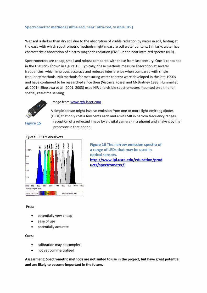
Image from www.rgb-laser.com
A simple sensor might involve emission from one or more light-emitting diodes
(LEDs) that only cost a few cents each and emit EMR in narrow frequency ranges,
reception of a reflected image by a digital camera (in a phone) and analysis by the
processor in that phone.
Pros:
• potentially very cheap
• ease of use
• potentially accurate
Cons:
• calibration may be complex
• not yet commercialised
Assessment: Spectrometric methods are not suited to use in the project, but have great potential
and are likely to become important in the future.
Figure 15
Figure 16 The narrow emission spectra of
a range of LEDs that may be used in
optical sensors.
http://www.lpi.usra.edu/education/prod
ucts/spectrometer/)
Page 19
Plant-based methods for estimating available soil water
Via their root network, plants extract water from soil and release it to the atmosphere in order to
grow. It is common in irrigated horticulture to estimate plant water status to improve irrigation
scheduling (Jones 2004).
Some methods estimate plant water status pre-dawn, in the absence of evaporative demand, when
plant water potential is approximately equal to the soil water potential. In the last few years,
continuous monitoring of plant water status has made this method more popular.
Other methods measure plant water stress during the day, with evaporative demand on the crop,
and measure reductions in sap flow and stomatal conduction (Woodruff and Meinzer 2011, Jones
2004), reductions in growth (Jones 2004), breakages in water-conducting tissues (Meinzer et al.
2009, Johnson et al. 2009) and heating of the crop canopy due to a reduction in transpiration and
associated evaporative cooling (Jackson et al. 1981).
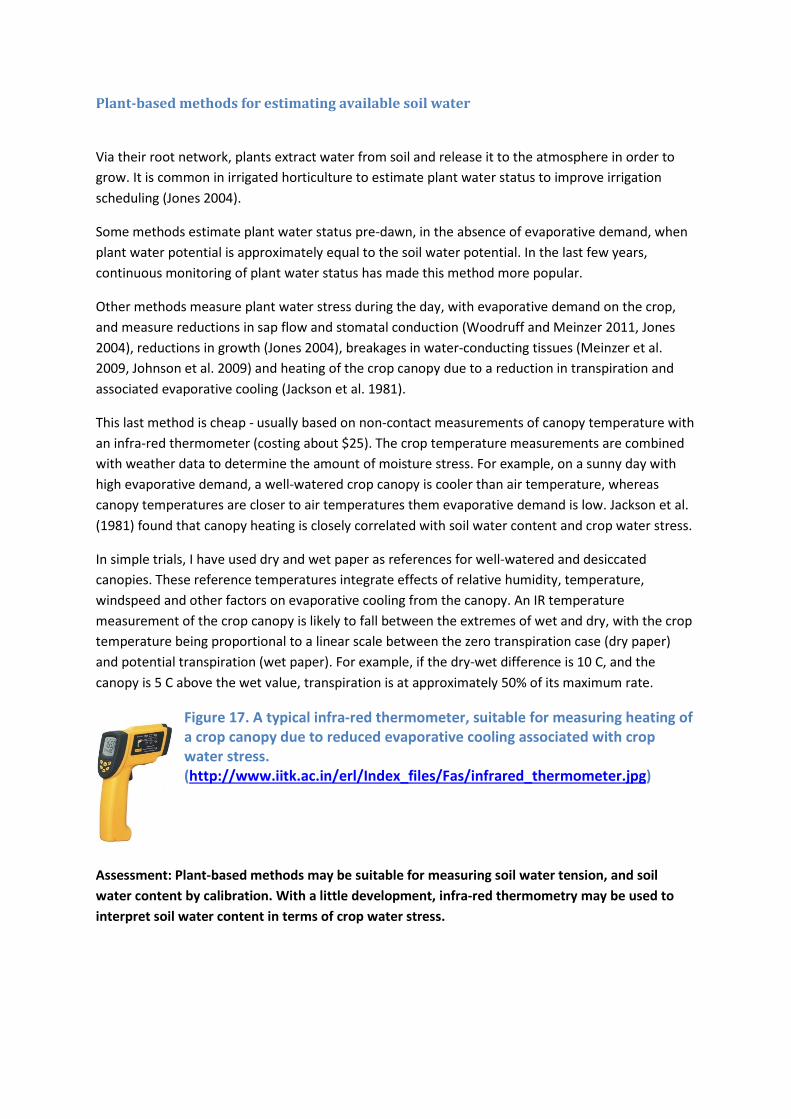
This last method is cheap - usually based on non-contact measurements of canopy temperature with
an infra-red thermometer (costing about $25). The crop temperature measurements are combined
with weather data to determine the amount of moisture stress. For example, on a sunny day with
high evaporative demand, a well-watered crop canopy is cooler than air temperature, whereas
canopy temperatures are closer to air temperatures them evaporative demand is low. Jackson et al.
(1981) found that canopy heating is closely correlated with soil water content and crop water stress.
In simple trials, I have used dry and wet paper as references for well-watered and desiccated
canopies. These reference temperatures integrate effects of relative humidity, temperature,
windspeed and other factors on evaporative cooling from the canopy. An IR temperature
measurement of the crop canopy is likely to fall between the extremes of wet and dry, with the crop
temperature being proportional to a linear scale between the zero transpiration case (dry paper)
and potential transpiration (wet paper). For example, if the dry-wet difference is 10 C, and the
canopy is 5 C above the wet value, transpiration is at approximately 50% of its maximum rate.
Figure 17. A typical infra-red thermometer, suitable for measuring heating of
a crop canopy due to reduced evaporative cooling associated with crop
water stress.
(http://www.iitk.ac.in/erl/Index_files/Fas/infrared_thermometer.jpg)
Assessment: Plant-based methods may be suitable for measuring soil water tension, and soil
water content by calibration. With a little development, infra-red thermometry may be used to
interpret soil water content in terms of crop water stress.
Page 20
Summary tables
Table 2. A summary of methods for measurement of soil water tension (SWT) or soil water content (SWC). Orange shading indicates a major
constraint to adoption of the method. Cost and complexity are based on weekly to monthly measurements (i.e. the App has no need for
sub-weekly measurements).
Type Commercial examples Method Range of measurement
Maximum bars of tension
Volume measured
Litres (approx.)
Cost and
complexity
SWT Jetfill/Irrometer Tensiometer (+gauge) <1 1 Low
SWT SoilSpec/TerraTech Tensiometer (no gauge) <1 1 Low
SWT NA Coring + hand feel 50 1 High
SWT Decagon WP4C Psychrometer minumum = 5 0.01 High
SWT Campbell 229 Thermal conductivity (porous block) 20 1 High
SWC NA Coring + drying (volumetric SWC) 20 1 High
SWC Push-probe Penetrometer 50 5 Low
SWC NA NIR/vis spectrum
(develop new sensor) 10 (?) 1 Medium
SWC Campbell TDR100 TDR 20 1 High
SWC Aquaflex TDR (+long sensor) 20 20 High
SWC Campbell 229 Soil thermal conductivity 20 1 High
SWC Geonics EM38 EMI 20 100 High
SWC NA “El-cheapo” EMI
(develop new sensor) 20 50 Medium
SWC Environscan/
C-probe/Diviner2000
EMI
(high frequency, down-tube sensor) 20 1 High
SWC Thetaprobe/Netafilm EMI
(high frequency, buried sensor) 5 1 High
SWC Decagon EC-5/
Vegetronix VH400
EMI
(high frequency, buried mini-sensor) 20 0.3 Medium
SWT (+SWC) Gypsum blocks EMI (very low frequency) 20 1 Medium
SWT (+SWC) GBLite/Watermark EMI (very low frequency) 3-5 1 Medium
Page 21
Bibliography
Bouyoucos, G.J. and Mick, A.H. 1947. Improvements in the plaster of Paris absorption blocks
electrical resistance method for measuring soil moisture under field conditions. Soil Science, 63:455-
465.
Bristow, K.L., Kluitenberg, G.J., Goding, C.J. and Fitzgerald, T.S. 2001. A small multi-needle probe for
measuring soil thermal properties, water content and electrical conductivity. Computers and
Electronics in Agriculture 31: 265-280.
Cummings, R.W. and Chandler, R.F.Jr. 1940. A field comparison of the electrothermal and gypsum
block electrical resistance methods with the tensiometer method for estimating soil moisture. Soil
Science Society of America Proceedings, 5:80-85.
Fletcher, J.S. 1939. A dielectric method for determining soil moisture. Soil Science Society of America
Proceedings 4:84-88.
Hummel, J.W., Sudduth, K.A. and Hollinger, S.E. 2001. Soil moisture and organic matter prediction of
surface and subsurface soils using an NIR soil sensor. Computers and Electronics in Agriculture 32:
149–165.
Jackson R.D., Idso S.B., Reginato R.J. and Pinter P.J. 1981. Canopy temperature as a crop water-stress
indicator. Water Resources Research 17: 1133–1138.
Johnson, D.M., F.C. Meinzer, D.R. Woodruff and K.A. McCulloh. 2009. Leaf xylem embolism, detected
acoustically and by cryo-SEM, corresponds to decreases in leaf hydraulic conductance in four
evergreen species. Plant, Cell and Environment 32: 828-836.
Jones, H.G. 2004. Irrigation scheduling: advantages and pitfalls of plant-based methods. Journal of
Experimental Botany 55: 2427-2436.
Meinzer, F.C., D.M. Johnson, B. Lachenbruch, K.A. McCulloh and D.R. Woodruff. 2009. Xylem
hydraulic safety margins in woody plants: coordination of stomatal control of xylem tension with
hydraulic capacitance. Functional Ecology 23: 922-930.
McKenzie, N., Bramley, R., Farmer, A., Janik, L., Murray, W., Smith, C. and McLaughlin, M. 2003.
Rapid soil measurement – a review of potential benefits and opportunities for the Australian grains
industry. Report for GRDC (Project CSO 00027).
Robinson, J.B., Silburn, D.M., Foley, J. and Orange, D. 2010. Root zone soil moisture content in a
Vertosol is accurately and conveniently measured by electromagnetic induction measurements with
an EM38. 19th World Congress of Soil Science, Brisbane.
http://www.iuss.org/19th%20WCSS/Symposium/pdf/2063.pdf
Shaw, B.J., H.R. Haise, and R.B. Farnsworth. 1942. Four years experience with a soil penetrometer.
Soil Science Society of America Proceedings 7:48–55.
Shibusawa, S., I Made Anom, S.W., Sato, S., Sasao, A. and Hirako, S. 2001. Soil mapping using the
real-time soil spectrophotometer. In ECPA 2001: 3rd European Conference on Precision Agriculture.
(S. Blackmore and G. Grenier, eds). Ecole Nationale Superieure Agronomique de Montpellier, France.
Page 22
Shibusawa, S., I Made Anom, S.W., Hache, C., Sasao, A. and Hirako, S. 2003. Site-specific crop
response to temporal trend of soil variability by the real-time spectrophotometer. In Precision
Agriculture: Proceedings of the 4th European Conference on Precision Agriculture. (J. Stafford and A.
Werner, eds). Wageningen Academic Publishers: Wageningen.
Slater, C.S. and Bryant, J.C. 1946. Comparison of four methods of soil moisture measurement. Soil
Science, 61:131-155.
Thornton, C.M., Cowie, B.A., Freebairn, D.M. and Playford, C.L. 2007. The Brigalow Catchment
Study: II. Clearing brigalow (Acacia harpophylla) for cropping or pasture increases runoff. Soil
Research 45: 496–511.
USDA. 1998. Estimating soil moisture by feel and appearance (revised 2001).
http://nmp.tamu.edu/content/tools/estimatingsoilmoisture.pdf
Viscarra Rossel, R.A. and McBratney, A.B. 1998. Laboratory evaluation of a proximal sensing
technique for simultaneous measurement of soil clay and water content. Geoderma 85: 19–39.
Williams, B.G. and Hoey, D. 1987. The use of electromagnetic induction to detect the spatial
variability of the salt and clay contents of soils. Australian Journal of Soil Research 25: 21–27.
Woodruff, D.R. and F.C. Meinzer. 2011. Water stress, shoot growth and storage of nonstructural
carbohydrates along a tree height gradient in a tall conifer. Plant Cell and Environment 34: 1920-
1930.
Page 23
Appendix 1
Economic costs and benefits of investing in collecting soil water
information
The costs and benefits of investing in soil water information will be highly variable between farms
and over time. The calculations below are a crude attempt to reveal possible savings and returns
from investing in modelling and measuring soil water in a particular scenario. The scenario involves
conditions similar to those found across the grain belt of northern Australia. Steps 1 and 2 describe
the background to the scenario and set out assumptions and intermediate results, while step 3
estimates savings ($/ha/year) and step 4 estimates the response in returns ($/ha/year).
1. Consider a farm of 2000ha with 50% cropped, so there is 1000ha of crop. For a conservative
estimate of variable costs of cropping of $100 per hectare, variable costs = $100,000 for the
cropped area. In northern Australia, cropped areas aren’t often put through a pasture ley, so
let’s assume that there is always 1000 ha of cropping each year. In southern Australia there
may be leys or long fallows that reduce the cropping intensity to 50%, reducing many of the
costs and returns from cropping by a factor of 2.
2. If, in any one year, 50% of the 1000 ha is subject to variable rates of inputs according to
weather and soil moisture conditions, there is $50,000 of variable-rate expenditure. The
50% area of variable inputs reflects that some areas might not need certain fertilisers, or
that the rate is determined by factors other than weather and soil moisture (e.g. chickpeas
don’t need N, barley needs less N than wheat, sorghum after chickpeas or long fallow needs
less N). Anything from 20 to 80% of the $25,000 may be spent on climate-responsive inputs
such as N fertiliser, seed, and some types of sprays. If we assume 50%, then the inputs cost
affected by soil-water are $25,000.
3. What percentage of the variable costs – can be saved with the App and soil sensors?
Research by Peter Hayman (ex NSW, now at SARDI) indicates that long-term average
management is remarkably profitable relative to climate-responsive management for
dryland farming. Residual benefits are one reason. For example, over-fertilising this year will
boost next year’s crop. Under-fertilising reduces yields, but saves money too. Based on the
available research, and assuming that over a long period, 10% of this expenditure would be
wasted without monitoring, the saving is $2,500 per year, or $2.50 per cropped hectare per
year.
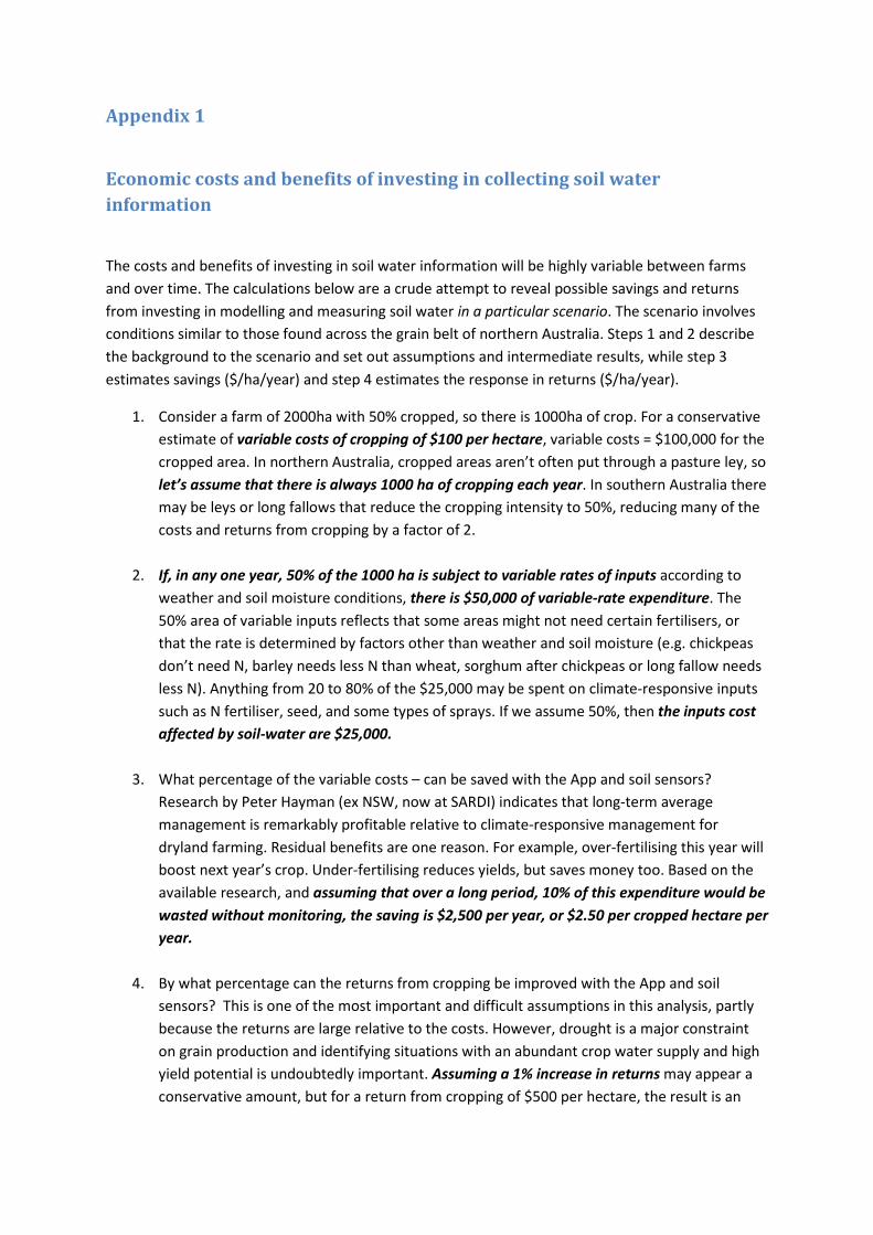
4. By what percentage can the returns from cropping be improved with the App and soil
sensors? This is one of the most important and difficult assumptions in this analysis, partly
because the returns are large relative to the costs. However, drought is a major constraint
on grain production and identifying situations with an abundant crop water supply and high
yield potential is undoubtedly important. Assuming a 1% increase in returns may appear a
conservative amount, but for a return from cropping of $500 per hectare, the result is an
Page 24
average increase of $5/ha/year. While this is only an educated guess, and is designed to be
conservative, it suggests that for 1000 ha of cropping the average increase in income per
year may be $5,000.
The total benefit of $7.50/ha/year may be put in perspective by comparison with using the phases
of the SOI to manage N fertiliser rates on wheat at Dalby, which has been estimated to increase
profit by $0.50/ha/year (data from Robinson and Butler, 2000).
Charlesworth (2000) estimated that the total cost of investing in soil water measurement is $4 to
$22 per hectare per year for a range of systems. These amounts were based on a 50 ha paddock and
spreading the capital costs over 10 years. Using the costing system of Charlesworth (2000) for an
area of 500ha, and a nominal set of capital and labour costs (Table 3), the annual costs of the 3
hypothetical systems are suitably low. However, I suggest that depreciating the capital cost over 10
years is optimistic. Conversely, in the future there will almost certainly be substantial improvements
in the technology and reductions in costs.
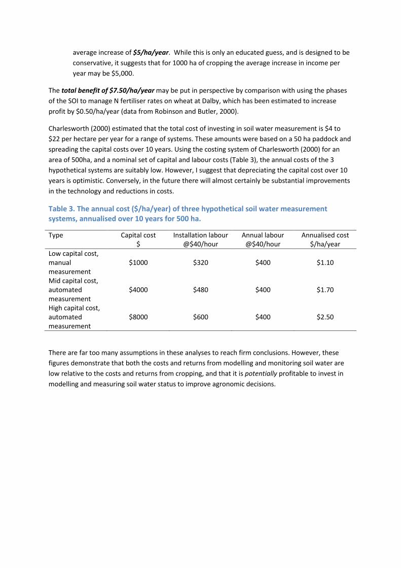
Table 3. The annual cost ($/ha/year) of three hypothetical soil water measurement
systems, annualised over 10 years for 500 ha.
Type Capital cost Installation labour Annual labour Annualised cost
$ @$40/hour @$40/hour $/ha/year
Low capital cost,
manual
measurement
$1000 $320 $400 $1.10
Mid capital cost,
automated
measurement
$4000 $480 $400 $1.70
High capital cost,
automated
measurement
$8000 $600 $400 $2.50
There are far too many assumptions in these analyses to reach firm conclusions. However, these
figures demonstrate that both the costs and returns from modelling and monitoring soil water are
low relative to the costs and returns from cropping, and that it is potentially profitable to invest in
modelling and measuring soil water status to improve agronomic decisions.
Page 25
Appendix 2
Soil water content and soil wetness
Those new to the science and technology of soil water are easily confused by the jargon and units of
measurement. Soil water availability may be expressed in centimetres of water, centimetres of
mercury, metres of water, kiloPascals, bars, pounds per square inch, megajoules per kilogram and
several less common units. The experts are sometimes confused as well.
In particular, it is not intuitive or obvious to many people that soil water content and soil wetness
are not the same thing. Soil water content (SWC) is, as the name suggests, how much water the soil
contains (usually on a gravimetric or volumetric basis), whereas soil wetness is how “available” the
water is in the soil. The relationship between the two differs between soils. Sand can be wet with
less water than other soils.
Soil wetness is often called the soil water tension, because moisture is ‘held’ to the soil by surface
tension – a product of polar nature of H2O. The less water in a soil, the greater the relative surface
area of the water (per unit mass) and the greater the tension between the water and the soil solids.
Matric tension (units of pressure, often kPa or bars), matric suction (units of pressure, where suction
is usually the inverse of tension, kPa or bars) and matric potential (units of energy per unit mass,
often MJ/kg) have equivalent meaning, and can be converted from one to the other.
SWC is often expressed as the volume of water (mL) in a 100 mL volume of soil - the % volumetric
water content. Perhaps the simplest method of measuring SWC is by weighing a sample of soil (A,
kg), drying it, and re-weighing (B, kg), and using this formula to calculate volumetric SWC:
SWC (%) = (B-A) / A x 100 x bulk density
The bulk density (kg/L) converts mass to volume.
Soil water tension (kPa) can be measured with tensiometers, pressure chambers, psychrometers and
artificial matrices (gypsum and ceramic blocks, filter paper, etc.). For tensiometers and pressure
chambers, water is extracted from soil in equilibrium with a vacuum (tensiometer) or pressure
(pressure chamber) acting against matric tension. Materials such as gypsum blocks and filter paper
have more-or-less constant relationships between their gravimetric or volumetric moisture content
and water tension. When placed in contact with soil, they come to equilibrium with the soil water
tension, and a measurement of their moisture content reveals the soil water tension. In the case of
gypsum and ceramic blocks, the moisture content is measured electronically, whereas for filter
paper it is measured gravimetrically. Psychrometers measure the water content of soil by cooling it
and optically detecting the dew point. Moist air has a higher dew point than dry air.
The relationship between SWC and SWT is known as the soil water retention function. To accurately
determine the relationship, soils of varying wetness have their SWC and SWT measured. In
particular, scientists and farmers often want to know the range of SWC at which plants are healthy
and able to use the soil water. The permanent wilting point (PWP), also known as the lower limit
(LL), is the SWC (%) where plants can no longer extract water and maintain their normal internal
water pressure. It is widely assumed to be the SWC when SWT is approximately 15 bars or 1.5 MPa.
This is a low value for coarse materials such as sand (e.g. 6% volumetric SWC) because the surface
Page 26
area is low, and water isn’t ‘held’ tightly. For clay, with orders of magnitude higher surface area, the
SWC for permanent wilting point is much greater (e.g. 25% volumetric SWC). See Table 44 for some
examples.
Table 4. A comparison of the soil water content (SWC, %) of different soils at similar
wetness (SWT, bars).
Soil type
Soil dryness (SWT) Sand Loam Clay
(bars of suction*) SWC (%) SWC (%) SWC (%)
Plant Wilting Point
(15 bars) 6 9 25
Field Capacity
(0.03 bars) 12 25 44
Saturation
(0 bars) 60 55 55
*Metric values of suction and tension are kiloPascals (kPa) and megaPascals (MPa). 1 bar is
approximately 100 kPa and 0.1 MPa.
More detailed technical information about soil water :
There is considerable variation between the SWC and SWT for soils of different texture, as
mentioned above. The relationship between SWC and SWT is called the “characteristic curve”
because it is characteristic of a particular soil. Fortunately, we don’t usually need to know exactly
the moisture characteristic curve of soils in order to make a fair estimate SWC or SWT from the
other, as the relationship depends on the proportions of fine and coarse materials in the soil, that in
turn determines the soil water tension at different moisture contents.
Page 27
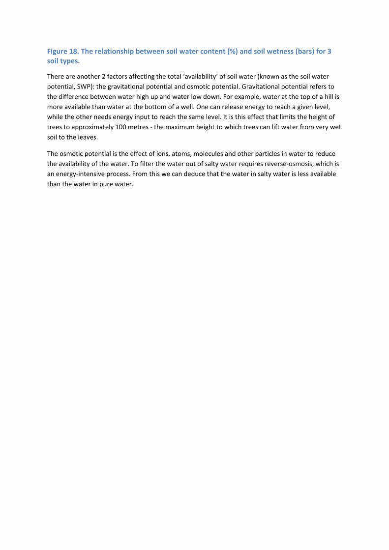
Figure 18. The relationship between soil water content (%) and soil wetness (bars) for 3
soil types.
There are another 2 factors affecting the total ‘availability’ of soil water (known as the soil water
potential, SWP): the gravitational potential and osmotic potential. Gravitational potential refers to
the difference between water high up and water low down. For example, water at the top of a hill is
more available than water at the bottom of a well. One can release energy to reach a given level,
while the other needs energy input to reach the same level. It is this effect that limits the height of
trees to approximately 100 metres - the maximum height to which trees can lift water from very wet
soil to the leaves.
The osmotic potential is the effect of ions, atoms, molecules and other particles in water to reduce
the availability of the water. To filter the water out of salty water requires reverse-osmosis, which is
an energy-intensive process. From this we can deduce that the water in salty water is less available
than the water in pure water.