This paper presents a complete formulation of the heatbalance method h~ a form that is suited to calculating coolingloads. The method was developed under ASHflAE researchproject RP-SZS, sponsored by TC 4o 1. The modeling assump-tions inherent in the heat balance method are presented, and ageneral model capable of representhzg the features of diversebuilding spaces is developed as the basis for the method. Themathematical foundation of the method is presented alongwith a pseudo-code description of the solution technique.Examples showing the use o,[ the method are included.
INTRODUCTION
ASHRAE TC 4.1 is sponsoring a research project entitled"Advanced Methods for Calculating Peak Cooling Loads" (RP-875)° This project began on August 1, 1995, and was to continuefor 20 months. In the work statement that led to the establishmentof that project, the committee states: "The current Handbook ofFundamentals Chapter 26 includes discussion of four coolingload methodologies (heat balance, weighting factors, CLTD/CLF, and TETD/TA), which is confusing to Handbook users andis undesirable. The heat balance method is the most scientificallyrigorous method. The description of this method in the Hand-book will be expanded to fully document the procedure."
The heat balance procedure is not new. Many energy calcu-lation pro~ams have used it in one form or another for manyyears. The first implementation that incorporated all theelements that form a complete method was NBSLD (Kusuda1967). The heat balance procedure is also implemented in boththe BLAST and TARP energy analysis programs (Walton1983). Unfortunately, the method has never been describedcompletely or in a form that is applicable to cooling load calcu-lations, This paper outlines the basics of the heat balance methodand discusses the translation of the method into a load calcula-tion procedure.
Why Is a Change Needed?
The three methods for calculating cooling loads presentedin some detail in the 199.3 ASHRAE Handbook-- Fundamentals(ASHRAE 1993) all spring from a basic heat balance model, butalong the way from the initial model to the final procedure, manysimplifying assumptions are made and the basic processes areessentially lost. The user ends up dealing with a "black box"concept such as CLTD instead of more traditionally fundamen-tal concepts such as surface temperatures, heat transfer coeffi-cients, and heat fluxes° In that regard, the procedures are severelyout of step with the rest of Fundamentals.
Further, the methods are not consistent within themselves.Consider the simple example given in chapter 26 of the 1993ASHRAE Handbook-- Fundamentals, shown in Figure 1. Thisshows the sensible cooling load calculated with the three meth-ods. There is clearly a significant difference among them, butsince the fundamental processes are completely hidden by eachprocedure, it is impossible to say which one is conservative andwhich one, if any, is risky. While the differences shown in Figure1 are significant, it is important to note what happens if theinstantaneous convective heat gains for all three methods at hour17 are subtracted from the total. These loads are identical for allthree methods and are about 23.6 kWo If this total, which does notenter into the procedures and is the same for all methods, issubtracted from the sensible cooling load, the loads due to proce-dure alone vary by up to 70%. It should be noted that the lighting
load for the example is very high and pr.obably does not reflectcurrent lighting load practice°
In addition to the obvious problems shown by the example,the procedures lack the capability for easily determining theeffect of making a simple change, such as building orientation oreven latitude, to say nothing of a more complex change, such aswindow type or wall construction.
Curtis O. Pedersen is a professor emeritus and Daniel E. Fisher and Richard J. Liesen are senior research engineers in the Mechanical andIndustrial Engineering Department at the University of Illinois, Urbana.
Sensible cooling loads from Chapter 26 of ASHRAE Fundamentals.
---0.- TF~t
What Is a Cooling Load?
When a heating, ventilating, and air-conditioning (HVAC)system is operating, the rate at which it is removing heat from aspace is the instantaneous heat extraction rate for’ that space atthat time. The concept of a design cooling load derives from theneed to determine an HVAC system size that under extremeconditions will provide a specified condition within the zoneserved. Usually the indoor boundary condition associated with acooling load calculation is a constant interior dry-bulb tempera-ture, but it could be a more complex function such as a thermalcomfort condition. What constitutes extreme conditions can beinterpreted in many ways but generally for an office would beassumed to be a clear sunlit day with high outdoor’ wet-bulb anddry-bulb temperatures, a high office occupancy, and a corre..spondingly high use of equipment and lights. Immediately it isapparent that even the boundary conditions for a cooling loaddetermination are subjective and require engineering judgment.For example, they might not involve constant indoor tempera-ture conditions but could occur in the rooming following a nighttime "setback" condition~ After the design boundary conditionsare agreed upon, the design cooling load represents the maxi-mum or peak heat extraction rate under the chosen design bound-ary conditions.
DESCRIPTION OF THE HEAT BALANCE MODEL
All calculation procedures involve sorne kind of model. Allmodels are approximate. The amount of detail involved in amodel depends very much upon the purpose of the model Thisis the reality of modeling: one chooses models that describe thevariables and parameters that are significant to the problem athand. The challenge is to make sure that no significant aspects ofthe process or device being modeled are excluded and at thesame time avoid unnecessary detail. While different levels of
model detail are useful for specific purposes, there is reasonablygood agreement among building physics researchers and prac-titioners that certain modeling simplifications are reasonable andappropriate. The most fundamental of these is that the air in thethermal zone can be modeled as well-stirred. This means it hasa uniform temperature throughout the zone because it mixes bymotion within itself. Some current research (ASHRAE RP-664)is concerned with determining the limits to this condition, but sofar it appears that the modeling assumption is quite valid over awide range of conditions. The truth of the matter is that the nextstep in complexity is a huge one that would require an enormousincrease in computational effort to rnodel a zone. Thus, the wellstirred model becomes the basis for’ most discussions of roomheat transfer.
The next major assumption is that the surfaces of the room(walls, windows, floor, etc.) can be treated as entities having
o uniform surface temperatures,¯ uniform long- and shortwave irradiation,o diffuse radiating surfaces, ando one-dimensional heat conduction within.
With those as a basis, it is possible to formulate fundamentalmodels for the various heat transfer and thermodynamic pro-cesses that occur. The resulting fon-nulation is called the "heatbalance model" and is described component by component inthe following sections. It is important to note that the forego-ing assumptions, although cornmon, are quite restrictive andset certain limits on the information that can be obtained fromthe model.
Elements of the Heat Balance Model
Within the framework of the assumptions outlined in thepreceding paragraphs, the heat balance model can be viewed as
460 ASHRAE Transactions: Symposia
FROM LIGHTS
SOLAR
INSIDE SURFACE~LANCE
TO ZONE
ANGE WITHOTHER A
SOURCES
INFILTRATION
EXHAUSTAIR
DUPLICATED FOR EACH SURFACE
CONVECTIONFROMINTERNAL
SOURCES
HVAC SYSTEMAIR
Figure 2 Schematic of heat balance processes in a zone.
four distinct processes: the outside face heat balance, the wallconduction process, the inside face heat balance, and the air heat
balance. The relationships between these processes are shown
schematically in Figure 2.
Figure 2 shows the heat balance process in detail for a single
opaque surface. The top part of the figure enclosed by the dashedline is repeated for each of the surfaces enclosing the zone. This
is indicated at the right of the figure. The process for transparent
surfaces would be similar to that shown but would not have the
absorbed solar component at the outside surface. Instead, it
would appear in the conduction process block. This absorbedcomponent splits into two parts: an inward-flowing fraction and
an outward-flowing fraction. These components would partici-
pate in the surface heat balances. The transparent surfaces
would, of course, provide the transmitted solar energy that isshown in the inside heat balance above.
The arrows indicate schematically where there is anexchange by having points on both ends and where the interac-tion is one way only by having a point only on one end. The fourmajor processes are shown as rounded blocks in the figure. Each
of these processes is described in the paragaphs that follow.
Outside Surface Heat Balance
The heat balance on the outside face of each surface is
q~.~ol + q’~wl¢ + q’~o,,v - q’£.o = 0
where
q~o = conduction flux into the wall, (q/A)
(1)
ASHRAE Transactions: Symposia 461
q~sot = absorbed direct and diffuse solar radiation flux,q"cwR= net longwave radiation flux exchange with the air
and surroundings, andq~o,,v = convective exchange flux with outside air.
All terms are positive for net flux to the face except the con-duction term, which is traditionally taken to be positive in thedirection from outside to inside of the walt.
Each of the heat flux terms in Equation 1 has been modeledin several ways, and in some fo~nulations the first three termsare combined by using an equivalent temperature called the "sol-air temperature." The models for the outside heat transfer arecovered in detail in a companion paper (McClellan 1997).
Wail Conduction Process
There are probably more ways to formulate the wallconduction process than any of the other processes. As a result,it is the topic that has received the most attention over the years.Among the possible ways to model this process are
o numerical finite difference,¯ numerical finite element,o transform methods, and° time series methods.
This process introduces part of the time dependence inherentin the load calculation process. It is shown schematically inFigure 3, which shows surface temperatures on the inside andoutside faces of the wall element and corresponding conduc-tive heat fluxes away fl’om the outside face and to the insideface. All four of the quantities are functions of time. The directformulation of the process has the two temperature functionsas input or known quantities and the two heat fluxes as outputsor resultant quantities.
In some formulations the surface heat transfer coefficientsare included as part of the wall element. Then the temperaturesin question are the inside and outside air temperatures. This is notan acceptable formulation since it hides the heat transfer coeffi-
ko
WallEl em ent
~ qki
Figure 3 Schematic of wall conduction process.
cients and prohibits changing them as airflow conditions change,and it also prohibits treating the internal longwave radiationexchange appropriately.
Since the heat balances on both sides of the element incor-porate both the temperature and heat flux, the solution techniquemust be able to deal with this simultaneous condition° From acomputational standpoint, two methods that have been usedwidely are a finite difference procedure and a time series methodusing conduction u’ansfer functions. Because of the computa-tional time advantage, the conduction transfer function formu-lation has been selected for the heat balance procedure presentedhere.
internal Heat Balance
The heart of the heat balance method is the internal heatbalance involving the inside faces of the zone surfaces. This heatbalance has many heat transfer components, and they are allcoupled. Both longwave (LW) and shortwave (SW) radiationare important, as well as wall conduction and convection to theair.
The inside face heat balance for’ each surface can be writtenas follows:
q’~wz + q"sw + q"tws + q;, + q;ot + q’£o,,v = 0
where
q~wx = net longwave radiant exchange flux between zonesurfaces,
net shortwave radiation flux to surface from lights,
longwave radiation flux from equipment in zone,
conduction flux through the wall,
transmitted solar’ radiation flux absorbed at surface,and
convective heat flux to zone air’.
q"sw =q"L WS=q"ki =q]~o z =
(2)
Each of these terms will be discussed briefly in the followingparagraphs and will be described in more detail in a compan-ion paper’ (Liesen 1997)~
Longwave Radiation Exchange Among Zone SurfacesThere are two limiting cases for internal LW radiation exchangethat are easily modeled.1. The zone air is completely transparent to LW radiation.2. The zone air completely absorbs LW radiation from the
surfaces within the zone.Most heat balance formulations treat air as completely transpar-ent. Then it does not participate in the LW radiation exchangeamong the surfaces in the zone. The other limiting case ofcompletely absorbing air has been used for load calculationsand also in some energy analysis calculations. This secondmodel is attractive because it can be formulated simply using acombined radiant and convective heat transfer’ coefficient fi’omeach surface to the zone air’ and thereby decouples the radiantexchange among surfaces in the zone. Because of this it isgenerally considered to be inferior to the first rnodel.
462 ASHRAE Transactions: Symposia
Furniture in a zone has the effect of increasing the amountof surface area that can participate in the radiant and convectiveheat exchanges. It also adds thermal mass to the zone. These twochanges affect the time response of the zone cooling load inopposite ways--the added area tends to shorten the responsetime, while the added mass tends to lengthen the response time.
The proper modeling of furniture needs further research, buta heat balance formulation at least allows the effect to bemodeled in a realistic manner by including the furniture surfacearea and thermal mass in the radiant and convective heatexchange process.
Longwave Radiation from Internal Sources The tradi-tional tnodel for this source defines a radiative/convective splitfor the heat introduced into a zone from equipment. The radiativepart is then distributed over the surfaces within the zone in someprescribed manner. This, of course, is not a completely realisticmodel and it departs from the heat balance principles. If it werehandled in a true heat balance model, the equipment surfaceswould be treated .just as other LW radiant sources within thezone. However, since information about the surface temperatureof equipment is rarely known, it is reasonable to keep the radia-tive/convective split concept even though it ignores the truenature of the radiant exchange. It should be noted that TC 4.1 hasinitiated a research prqject to determine radiative/convectivesplits for many additional equipment types. This will tend toinstitutionalize the radiative/convective split model further,although the research will address the exchange problem in alimited way.
Shortwave Radiation from Lights The short wavelengthradiation from lights is usually assumed to be distributed over thesurfaces in the zone in some prescribed manner. The new proce-dure will retain this approach but will allow the distribution func-tion to be changed.
Transmitted Solar Energy ASHRAE TC 4.5, Fenestra-tion, is currently revising the calculation procedure for determin-ing transmitted soIar energy. They are proposing to use the solarheat gain coefficient (SHGC) directly rather than relate it to thatfor a double-strength glass as is done when using the shadingcoefficient (SC). This approach was described by Wright (1995).The problem with this plan is that the SHGC includes both thetransmitted solar energy and the inward-flowing fraction of thesolar radiation absorbed in the window. In keeping with the heatbalance formulation, this latter part should be added to theconduction component so that it can be included in the insidesurface heat balance°
Transmitted solar radiation is also distributed over thesurfaces in the zone in a prescribed manner. It would be possibleto calculate the actual position of beam solar radiation, but thatwould involve partial surface irradiation, which is inconsistentwith the rest of the zone model that assumes uniform conditionsover an entire surface.
The current cooling load procedures incorporate a set ofprescribed distributions. Since the heat balance approach candeal with any distribution function, the sensitivity of the load tothis function can be investigated, and principles for selecting
logical distributions under different conditions can be devel-oped.
Convection to Zone Air The inside convection coefficientspresented in ASHRAE Fundamentals and used in most loadcalculation procedures and energy programs are based on veryold natural convection experiments and do not accuratelydescribe the heat transfer coefficients that are present in amechanically ventilated zone. In the current load calculationprocedures, these coefficients are buried in the procedures andcannot be changed. A heat balance formulation keeps them asworking parameters. In this way, new research results such asthose from RP-664 can be incorporated into the procedures. Itwill also permit one to determine the sensitivity of the load calcu-lation to these parameters.
Air Heat Balance
In heat balance formulations aimed at determining coolingloads, the capacitance of the air in the zone is neglected and theair heat balance is done as a quasi-steady balance in each timeperiod. There are four contributors to the air heat balance. Theyare convection from the zone surfaces, convective parts of inter-nal loads, infiltration and ventilation, and the HVAC system air:
qconv + qce + qlv + q~ys = 0 (3)
where
qcE
q~v
= convection heat transfer from the surfaces,
= convective part of internal loads,
= sensible load due to infiltration and ventilation air,and
qsys = heat transfer to/from the HVAC system.
qconv, the convection from zone surfaces, is the sum of all theconvective heat transfer quantities from the inside surface heatbalance. This comes to the air via the convective heat transfercoefficient on the surfaces.
qCE, the convective parts of internal loads, is the companionto the radiant contribution from internal loads described previ-ously. It is added directly into the air heat balance. Such a treat-ment also violates the tenets of the heat balance approach sincesurfaces producing the internal loads exchange heat with thezone air through normal convective processes. However, onceagain, the details required to include this level of detail into theheat balance m’e generally not available, so including it into theair heat balance directly is a reasonable approach.
In keeping with the well-stirred model for the zone air, anyair that enters by way of ventilation or infiltration, q~v, is imme-diately mixed with the zone air. The determination of the amountof infiltration air is quite complicated and subject to significantuncertainty. Sometimes it is related to the indoor-outdoortemperature difference and wind speed; however it is deter-mined, it is added directly to the air heat balance.
The conditioned air that enters the zone from the HVACsystem and provides q.~.s is also mixed directly with the zoneThis is consistent with the well-stirred model.
ASHRAE Transactions: Symposia 463
THE GENERAL ZONE FOR LOAD CALCULATION
The heat balance procedure as described has been applied toenergy calculation programs, which also have the capability todo load calculations but frequently are perceived to be toocumbersome to be used for that purpose. Thus there is a need fora framework that is tailored to a single thermal zone. The defi-nition of a thermal zone is sometimes confusing but, in a way, theheat balance model helps to define it. Recall that one of the basicassumptions is that the air is well stirred, that is, at a uniformtemperature. So, the test for determining what part of a buildingcan be called a thermal zone comes down to how the temperatureis going to be controlled. If air is being circulated through anentire building or an entire floor in such a way that it is reasonableto consider it well stirred, then the entire building or floor couldbe a thermal zone. On the other hand, if there are different controlschemes for each room, then it may be necessax2¢ to considereach room as a separate thermal zone. The framework needs tobe flexible enough to accommodate any zone arrangement, butthe heat balance aspect of the procedure also requires that acomplete zone be described. Accordingly, a generalized 12-surface zone is used as a basis to present the method. This zoneconsists of four walls, a roof or ceiling, a floor, and a thermalmass surface as shown in Figure 4. Each of the walls and the roofcan include a window (or skylight, in the case of the roof). Thismakes a total of 12 surfaces, any of which may have zero area ifit is not present in the zone to be modeled.
The heat balance processes for this general zone are fon-nu-lated for a 24-hour steady periodic condition. The variables ofthe problem are the inside and outside face temperatures of the12 surfaces plus either the HVAC system energy required tomaintain a specified air temperature or the air temperature, if thesystem capacity is specified, for each of the 24 hours. This makesa total of 25 x 24 or 600 variableso While it would be possibleto set up the problem for a simultaneous solution of these vari-ables, the relatively weak coupling of the problem from one hourto the next permits a double iterative approach, which incorpo-rates an iteration through all the surfaces in each hour and thenan iteration through the 24 hours of the day~ This automatically
~Roof and Skylight
Back Wall and Window
Floor
Front Wall/Windowand lhermal Massare not shown
Figure 4 Schematic view of general heat balance zone.
reconciles the nonlinear aspects of the surface radiativeexchange and the other heat flux terms.
The heat balance procedure based on this generalized zoneis described mathematically in the next section.
Because it links tbe outside and inside heat balances, thewall conduction process plays a key role in the overall heatbalance procedure. It is the process that regulates the time depen-dence of the cooling load. For the heat balance procedurepresented here, the wall conduction process will be formulatedusing conduction transfer functions (CTF). These relate conduc-tive heat fluxes to the current and past surface temperatures andthe past heat fluxes. The general form is
The subscript following the comma indicates the time periodfor the quantity in terms of the time step 6. The first terms inthe series have been separated from the rest in order to facili-tate solving for the current temperature in the solution scheme.
The two summation limits, nz and nq, are dependent on thewall constmctiou and somewhat dependent ors the scheme usedfor calculating the CTFs. If nq = 0, the CTFs are generallyreferred to as response factors, but then theoretically nz is infi-nite. The values for nz and nq are generally set to minimize theamount of computation. A development of CTFs can be found inHittle (1979).
464 ASHRAE Transactions: Symposia
The Heat Balance Equations
The primary variables in the heat balance for the generalzone are the 12 inside face temperatures and the 12 outside facetemperatures at each of the 24 hours° We will assign the firstsubscript, i, as the surface index and the second subscript,j, as thehour index, or, in the case of CTFs, the sequence index° Then, theprimary variables are:Tsol.j = outside face temperature, i= 1, 2 ....
12;j= 1, 2 .... 24Tsii.j = inside face temperature, i = 1, 2 ....
12;j = 1, 2 .... 24.
In addition, we have the variable qs~,sj= cooling load,j = 1, 2 ...24.
Equations 1 and 5 are combined and solved for Tso to produce12 equations applicable in each time step:
outside convection coefficient, introduced by usingq"co,,v = hco(To- T,o)
This equation shows the need for separating the first term ofthe CTF series, Zi,o, since in that way the contribution of thecurrent surface temperature to the conduction flux can becollected with the other terms involving that temperature. Acompanion paper ~cClellan 1997) presents alternative equa-tions for the outside temperature, depending on the outside heattrar~sfer model that is chosen.
Equations 2 and 4 are combined and solved for 7~i toproduce the next 12 equations:
hci = convective heat transfer coefficient on the inside,obtained from q’~o,,,,, = hci(Ta - Tsi)"
Note that in Equations 6 and 7, the opposite surface tempera-ture at the current time appears on the right-hand side° The twoequations could be solved simultaneously to eliminate thosevariables. Depending on the order of updating the other termsin the equations, this can have a beneficial effect on the solu-tion stability.
The remaining equation comes from the air heat balance,Equation 3. This provides the cooling load, q.~,s, at each timestep:
InEquation 8, the convective heat transfer term is expanded toshow the interconnection between the surface temperaturesand the cooling load.
Overall HB Iterative Solution Procedure
The iterative HB procedure is quite simple. It consists of aseri6s of initial calculations that proceed sequentially followedby a double iteration loop. This is shown in the procedure shownbelow.
1. Initialize areas, properties, and face temperatures for allsurfaces, 24 hours.
2~ Calculate incident and transmitted solar flux for allsurfaces and hours.
3. Distribute transmitted solar energy to all inside faces, 24hours.
4. Calculate internal load quantities for all 24 hours
5. Distribute LW, SW, and convective energy from inter-nal loads to all surfaces for all hours.
6. Calculate infiltration and ventilation loads for all hours.
7o Iterate the heat balance according to the followingscheme:
For Day= 1 to Maxdays
Forj =1 to24 {hours in the day}
For Surfacelter=l to Maxlter
For i=l to 12 {The twelve zone surfaces}Evaluate Equations 6 and 7.
Next i
Next Surfacelter
Evaluate Equation 8.
Next j
If not converged, Next Day
8. Display Results
It has been found that four or six surface iterations are gener-ally sufficient to provide convergence. The solution of Equations6 and 7 may present convergence problems under some circum-stances. If so, it may be necessary to use an under-relaxationcoefficient when updating Equation 7 or change the algorithm toprovide a simultaneous solution of the two equations. Also, theform of the longwave radiant exchange flux can significantlyaffect the stability. A companion paper (Liesen 1997) examinesseveral different ways to calculate that term and presents someinsights on their effect on the solution.
The convergence check on the day iteration should be basedon the difference between the inside and the outside conductive
ASHRAE Transactions: Symposia 465
heat flux terms, q~. A limit, such as requMng the differencebetween all inside and outside flux terms to be less than 1% ofeither flux, seems to work well.
INPUTS REQUIRED FOR HEATBALANCE PROCEDURE
Previous methods for calculating cooling loads haveattempted to simplify the procedure by precalculating cases andgrouping the results with various correlating parameters. Thisgenerally tended to reduce the amount of information required toapply the procedure. In the case of the heat balance procedure, noprecalculations are made, and the procedure requires a fairlycomplete description of the zone.
Global information
Because the procedure incorporates a solar’ calculation,some global information is required. This includes latitude,longitude, time zone, month, day of month, north axis of thezone, and the zone height. Additionally, if the user wants to takefull advantage of the flexibility of the method to incorporate, forexample, variable outside heat transfer coefficients, it would benecessary to specify such things as wind speed, wind direction,and terrain roughness. These variables and others would almostcertainly be defaulted to some reasonable set of values, but theflexibility remains.
Wall Information (Each Wall)
Since the walls are involved in three of the fundamentalprocesses (external and internal heat balance and wall conduc-tion), each wall of the zone requires a fairly large set of variables.They include
o facing angle with respect to building north,o tilt (degrees from horizontal),o area,o solar absorptivity outside,° longwave emissivity outside,o shortwave absorptivity inside,o longwave emissivity inside,o exterior boundary temperature code,o external roughness, ando layer-by-layer construction information.
Again, some of these can be defaulted, but they are change-able and indicate the more fundamental character of the heatbalance method since these parameters are related to true heattransfer’ processes.
Window information (Each Window) .............
The situation for windows is similar’ to that for walls, but thewindows require some additional information because of theirrole in the solar load. The necessary parameters include
o area,o normal solar’ transmissivity,
o normal SHGC,¯ normal total absorptivity,¯ longwave emissivity outside,o longwave emissivity inside,° surface-to-surface thermal conductance,o reveal (for solar shading),¯ overhang width (for solar shading), ando distance from overhang to window (for solar shading).
It can be seen that considerable design flexibility is possiblefor windows.
Roof and Floor Details
The roof and floor surfaces are specified similarly to walls.The main difference is that the ground outside boundary condi-tion will probably be specified more often for a floor.
Thermal Mass Surface Details
The general formulation includes an "extra" surface, whichis called a thermal mass surface, but it can serve several func-tions. It is included in the radiant heat exchange with the othersurfaces in the space but is only exposed to the inside air convec-tive boundary condition. As an example, one of the uses of thissurface would be to account for the movable partitions within aspace. The construction of the partitions is specified layer’ bylayer similarly to walls, and those layers store and release heatvia the same conduction mechanism as walls. As a general defi-nition, the extra thermal mass surface should be sized to r’epre-sent all of the surfaces within the space that are exposed to the air’mass, except the walls, roof, floor’, and windows. In the fo~nu-lation, both sides of the thermal mass participate in the exchange.
Internal Heat Gain Details
The space can be subjected to several internal heat sources.They are people, lights, electrical equipment, and infiltration. Inthe case of infiltration, the energy is assumed to go immediatelyinto the air heat balance, so it is the least complicated of the heatgains. For the others, it is necessary to specify several parame-ters. These include the following fi’actions:
the fraction of the heat gain that is sensible energy,the fraction of the heat gain that is latent energy,the fi’action of the energy that enters as short wavelengthradiation,the fraction of the energy that enters as long wavelengthradiation,the fraction of the energy that enters the air immediatelyas convection,the activity level of the people, andthe fi’action of the energy of the lighting heat gain thatgoes directly to the return air.
Radiant Distribution Functions
As mentioned previously, the generally accepted assump-tions for the heat balance method include specifying the distri-
466 ASHRAE Transactions: Symposia
bution of radiant energy from several sources to the surfaces thatenclose the space. This requires a distribution function that spec-ifies the fraction of the total radiant input that is absorbed by eachsurface. The types of radiation that require distribution functionsare
o long wavelength radiation from equipment and lights,¯ short wavelength radiation from lights, and
¯ transmitted solar radiation.
Other Required Information
Additional flexibility is included in the model so that resultsof fundamental research can be incorporated easily. Thisincludes the capability to specify such things as
heat transfer coefficients/convection models,solar coefficients, and
sky models.
The amount of information indicated in the preceding sectionsmay seem extensive, but in most routine applications of themethod, many of the parameters can be set to default values, ~eatlyreducing the amount of information required. However, all of theparameters listed can be changed when necessary to fit unusualcircumstances or when additional information is obtained°
THE HANDBOOK EXAMPLE USINGHEAT BALANCE PROCEDURE
The heat balance procedure described in a previous sectionhas been implemented in both Fortran90 and Basic. Thosepro~ams have been used to calculate the example fromASHRAE Fundamentals described previously. The results areshown in Figure 5. The results using the other methods fromFigure 1 are shown for reference. Without extensive experimen-tal verification, it is not possible to say that the heat balance resultis correct, but it does stand to reason that using the complete
’~.a30
Figure g ASHRAE Fundamentals example using heatbalance procedure.
Figure6 Inside sutface temperatures for ASHRAEHandbook example°
procedure that the other methods only approximate shouldprovide a better result.
The other advantage of using the complete heat balanceprocedure is that additional useful information about the perfor-mance of components is available, not just the final cooling toad.For example, Figure 6 shows some of the inside surface temper-atures for the walls and windows of the example. The high calcu-lated temperatures indicate that additional insulation might beappropriate for this building.
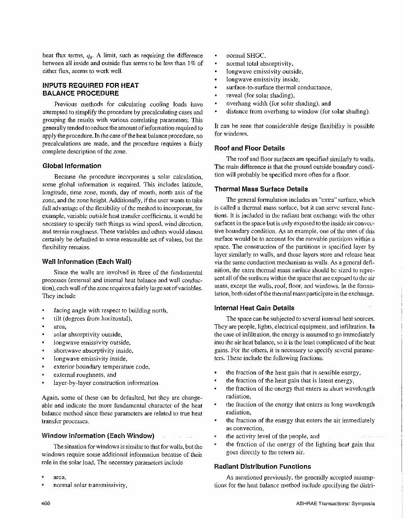
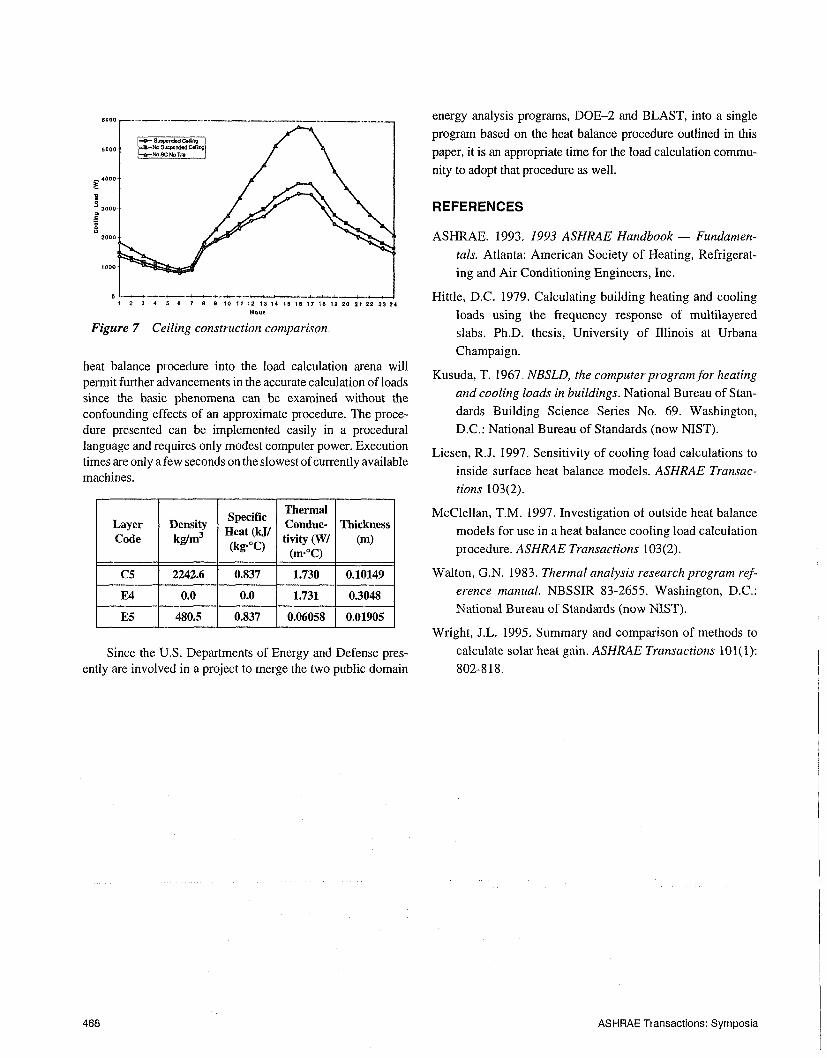
Another example shows the procedure being used to deter-mine how changes to the building structure can affect the coolingload. The results from modeling a simple zone are shown inFigure 7. The zone was a southwest comer zone with windowson the south and west walls. The zone originally was modeledwith a suspended ceiling in the roof by using a roof constructionconsisting of a layer of concrete, an air space, and a layer of ceil-ing tile. The properties of the layers are given in the table below.Note that the thermal resistance of the air layer (E4) is specifiedby the ratio of thickness to thermal conductivity (L/k).
The heat balance procedure was run with the three walllayers as shown. Then it was rerun without the air layer (E4).This would be equivalent to having the ceiling tile glued to thebottom of the concrete. It was then run again with only theconcrete layer (C5). These runs are labeled Suspended Ceiling,No Suspended Ceiling, and No SC No Tile, respectively, in thelegend. It is clear that the air space in the suspended ceiling hassome effect, but the more significant effect comes when the insu-lation of the ceiling tile is not present. It would be easy to inves-tigate the effect of reducing the radiant transfer across the airlayer resulting from changing the surface emissivities. Thiswould change the effective thermal resistance of the air layer.
CONCLUDING REMARKS
This paper has presented a complete formulation of a heatbalance procedure for determining cooling loads. The funda-mental assumptions involved in the zone model have beenpresented and their reasonableness discussed. Incorporating the
ASHRAE Transactions: Symposia 467
5000
~4000
Figure 7 Ceiling construction comparison.
heat balance procedure into the load calculation arena willpermit further advancements in the accurate calculation of loadssince the basic phenomena can be examined without theconfounding effects of an approximate procedure. The proce-dure presented can be implernented easily in a procedurallanguage and requires only modest computer power. Executiontimes are only a few seconds on the slowest of currently availablemachines.
LayerCode
C5
Densitykg/m3
2242.6
SpecificHeat (k J/(~g.°c)
0.837
ThermalConduc-tivity (W/(m.°C)
1.730
Thickness(m)
0.10149
E4 0.0 0.0 1.731 0.3048
E5 480.5 0.837 0.06058 0.01905
Since the U.S. Departments of Energy and Defense pres-ently are involved in a project to merge the two public domain
energy analysis programs, DOE-2 and BLAST, into a single
progam based on the heat balance procedure outlined in this
paper, it is an appropriate time for the load calculation commu-nity to adopt that procedure as well.
REFERENCES
ASHRAE. 1993. 1993 ASHRAE Handbook -- Fundamen-
tals. Atlanta: American Society of Heating, Refi’igerat-ing and Air Conditioning Engineers, Inc.
Hittle, D.C. 1979. Calculating building heating and cooling
loads using the frequency response of multilayered
slabs. Ph.D. thesis, University of Illinois at UrbanaChampaign.
Kusuda, T. 1967. NBSLD, the computer program for heatingand cooling loads in buildings. National Bureau of Stan-
dards Building Science Series No. 69. Washington,
D.C.: National Bureau of Standards (now NIST).
Liesen, R.J. 1997. Sensitivity of cooling load calculations to