Did FIN 48 improve the predictive ability of tax expense? Evidence from a comparison with IFRS firms Cristi A. Gleason Henry B. Tippie College of Business The University of Iowa [email protected]Kevin S. Markle Henry B. Tippie College of Business The University of Iowa [email protected]Jane Z. Song J.M. Tull School of Accounting University of Georgia [email protected]July 2018 Abstract The FASB introduced FIN 48 (ASC 740-10) to increase relevance and comparability in the reporting of uncertain tax positions. Using a difference-in-differences design, we examine the effect of FIN 48 on the predictive ability of tax expense for cash taxes paid for U.S. firms and find that the ability of GAAP tax expense to predict future tax cash flows incrementally improved under FIN 48. Additionally, we find that the improvements in the predictive ability of tax expense are confined to firms with higher probability of audit, which are likely less affected by the assumption of certain audit introduced by FIN 48. We find no evidence that FIN 48 reduced the predictive ability of tax expense for firms with a low likelihood of being audited. Furthermore, the improvements in predictive ability are attributable to current, not deferred, tax expense. We conduct a series of robustness tests to mitigate concerns about effects of the time period and sample composition. Because our research design isolates the effects of the change in standard and holds the underlying complexity of the tax process constant, we can attribute the improved predictive ability of tax expense to FIN 48. Our findings suggest that FIN 48 improved the relevance of tax expense for some U.S. firms. Keywords: FIN 48, IFRS, IAS 12, relevance, predictive ability, tax expense, cash taxes paid We appreciate helpful comments and suggestions from Jennifer Blouin (discussant), Lil Mills, Erin Towery, Ryan Wilson, and meeting participants at the 2017 NTA Annual Conference, and workshop participants at the University of Connecticut and the University of Illinois.
Transcript
Did FIN 48 improve the predictive ability of tax expense?
Evidence from a comparison with IFRS firms
Cristi A. Gleason Henry B. Tippie College of Business
The FASB introduced FIN 48 (ASC 740-10) to increase relevance and comparability in the reporting of uncertain tax positions. Using a difference-in-differences design, we examine the effect of FIN 48 on the predictive ability of tax expense for cash taxes paid for U.S. firms and find that the ability of GAAP tax expense to predict future tax cash flows incrementally improved under FIN 48. Additionally, we find that the improvements in the predictive ability of tax expense are confined to firms with higher probability of audit, which are likely less affected by the assumption of certain audit introduced by FIN 48. We find no evidence that FIN 48 reduced the predictive ability of tax expense for firms with a low likelihood of being audited. Furthermore, the improvements in predictive ability are attributable to current, not deferred, tax expense. We conduct a series of robustness tests to mitigate concerns about effects of the time period and sample composition. Because our research design isolates the effects of the change in standard and holds the underlying complexity of the tax process constant, we can attribute the improved predictive ability of tax expense to FIN 48. Our findings suggest that FIN 48 improved the relevance of tax expense for some U.S. firms. Keywords: FIN 48, IFRS, IAS 12, relevance, predictive ability, tax expense, cash taxes paid
We appreciate helpful comments and suggestions from Jennifer Blouin (discussant), Lil Mills, Erin Towery, Ryan Wilson, and meeting participants at the 2017 NTA Annual Conference, and workshop participants at the University of Connecticut and the University of Illinois.
“This Interpretation will result in increased relevance and comparability in financial reporting of income taxes because all tax positions accounted for in accordance with Statement 109 will be evaluated for recognition, derecognition, and measurement using consistent criteria.”
— FASB Summary of Interpretation No. 48
1. Introduction
The measurement and reporting of uncertain tax positions under U.S. GAAP changed
in 2007 with the implementation of FASB Interpretation Number 48 (FIN 48). Since FIN 48
was implemented, multiple studies have examined the effects of the change in standard and
found evidence suggesting that the FASB’s stated intentions of increased relevance
(Robinson, Stomberg, and Towery 2016) and comparability (De Simone, Robinson, and
Stomberg 2013) have not been realized. We extend this literature by studying the effect of
FIN 48 on a principal component of relevance, the ability of GAAP tax expense to predict
future tax cash flows.1
Although improving relevance was one of standard setters’ objectives in issuing FIN
48, it remains an open empirical question whether the objective has been met. Survey
evidence collected by the Financial Accounting Foundation (FAF) indicates that
practitioners and providers believe that the information reported under FIN 48 is more
relevant. However, survey participants also indicated that they believe that reserves are larger
than settlements because of both to the estimation rules and complex recognition and
derecognition requirements introduced by FIN 48 (FAF 2012). The FAF noted that post-FIN
48 reserves “may not be predictive or confirmatory of future cash flows” because of the
benefit recognition approach used in FIN 48.
1 Another aspect of relevance articulated in FASB Concept Statement No. 8 is confirmatory value.
2
Empirical evidence on the effect of FIN 48 on the relevance of the tax information in
financial statements is also mixed. Using a sample of U.S. firms, Robinson, Stomberg, and
Towery (2016) compare the ability of tax expense to predict future tax cash flows before and
after FIN 48 and find no evidence that FIN 48 improved tax expense relevance, on average.
In contrast, Ciconte et al. (2016), also using a sample of U.S. firms, find that tax reserves
post-FIN 48 do not appear to be systematically over- or under-reserved, suggesting that they
are relevant. For a sample of U.S. firms with material IRS audit assessments or settlements,
Gleason, Mills, and Nessa (2017) find that the comparability of tax reserves improved after
FIN 48 was implemented.
We take steps toward reconciling the mixed findings in prior studies by using a
difference-in-differences design with a control sample of firms reporting under IFRS.
Financial accounting for income tax under IFRS remained stable during the development and
implementation of FIN 48 under U.S. GAAP, which allows us to assess changes to the
predictive ability of tax expense attributable to FIN 48. Additionally, IFRS permits greater
discretion over the reporting of tax uncertainties, which allows us to evaluate critiques that
the stringent guidelines under FIN 48 lead to poorer quality reserves because they hamper
managers’ ability to convey private information and experience. Under FIN 48, firms are
required to apply a two-step process to determine the recognition and measurement of
uncertain tax positions, without considering the probability of audit. Because IFRS provides
no direct guidance on accounting for tax uncertainties, firms reporting under IFRS employ
an expected value approach, under which audit probability is considered.
Using a treatment sample of U.S. firms reporting under U.S. GAAP and a control
sample of non-U.S. firms reporting under IFRS from 2006-2014, we find that the ability of
3
tax expense to predict future tax cash flows three years later improved under FIN 48. Because
we benchmark U.S. firms against firms unaffected by FIN 48, our research design isolates
the effects of the change in standard while holding constant the underlying complexity of the
tax process. Therefore, we can attribute the relative improvement in the predictive ability of
tax expense to FIN 48.
Because our control sample consists of IFRS firms and IFRS was mandated in 2005,
our pre-FIN 48 period contains just one year. We perform several additional tests to mitigate
concerns about our short pre period. First, to ensure that our results are not due to systematic
patterns in the relation between tax expense and cash taxes unrelated to FIN 48, we conduct
a pseudo-event (falsification) analysis in which we redefine the FIN 48 enactment year as
2009, 2010, and 2011. We find no significant incremental effect of the pseudo-event years
on the relative predictive ability of tax expense. Second, we extend the pre-period to 2002,
before IFRS became mandatory for our non-U.S. sample, and find our results become weaker
(due to noise created by firms reporting on local GAAP) but remain significant. In other
robustness tests, we find our results continue to hold after we adjust tax expense for stock-
based compensation, when we drop years containing the financial crisis, and when we limit
the sample to firms with data in both the pre- and post-FIN periods.
To provide more evidence on the effect of changes in the measurement of tax reserves
under FIN 48, we partition firms based on the likelihood the firms would be audited by tax
authorities. We find that the improvement in the predictive ability of tax expense is
concentrated in firms with higher ex ante audit probability, which are less likely to be
affected by the assumption of certain audit introduced by FIN 48. We find no improvement
in the predictive ability of tax expense for small firms with lower probabilities of audit and
4
detection. These firms have no change. One possibility is the increased management and
auditor scrutiny of tax reserve judgments results in an improvement that offsets the effect of
ignoring audit and detection probability.
Our study contributes to the literature on the impact and effectiveness of FIN 48. We
also contribute to the literature on the differences between U.S. GAAP and IFRS and
implications for the convergence effort. On June 7, 2017, the IASB issued an interpretation
of IAS 12, IFRIC 23 Uncertainty over Income Tax Treatments. For fiscal years beginning
after January 2019, firms reporting under IFRS will implement a benefits recognition
approach similar to FIN 48 when accounting for uncertain tax benefits. Our analysis helps
inform standard-setters about the possible effects of the new interpretation on the relevance
of tax expense.
2. Prior literature and hypothesis development
FIN 48 was introduced to improve the relevance and comparability of financial
reporting for income taxes and provide more information in financial statements about
uncertainty in income tax assets and liabilities (FASB 2006). Despite its professed purpose,
practitioners argue the complexity and judgment inherent in the measurement process leads
to reserving for tax liabilities that are not expected to be paid and to disclosures which are
not comparable across firms (Tysiac 2012, Guertin 2012). In 2011, the Tax Executive
Institute issued comments to the Financial Accounting Foundation (FAF) that the standard
fails to “reflect the knowledge, experience, and judgement of the company because the
inability to take into account the dynamic process [of an audit] and reflect the firm’s
judgment about the overall outcome” results in overstated tax liabilities (Robinson,
Stomberg, and Towery 2016). In the FAF’s Post-Implementation Review (PIR) of the
5
standard in 2009, the review team reported that “preparers and practitioners generally do not
believe FIN 48 resolves the issues underlying the need for the standard” (Tysiac 2012).
Whether FIN 48 achieved the goal of enhancing the relevance of reported tax expense is still
a matter of contention. Our study focuses on changes in the relevance of income tax
information following FIN 48 and specifically, changes in the predictive value of income tax
expense for future tax cash flows.
Assessing the impact of FIN 48 is hampered by several challenges. First, prior to FIN
48, tax reserves were not consistently accounted for or disclosed in financial statement
footnotes (Gleason and Mills 2002, Blouin and Tuna 2007, Blouin et al. 2010). For example,
probability thresholds for recognition and the classification of the liability as current or long-
term varied significantly in practice (e.g., Gleason 2007). The endogenous nature of pre-FIN
48 disclosure limits the generalizability of inferences based on samples drawn from
disclosing firms. Second, FIN 48 was effective for fiscal years beginning after December 15,
2006. Only a single fiscal year precedes the 2008 financial crisis, which decreases the
comparability of the pre- and post-FIN 48 time periods in ways that are likely to be correlated
with firms’ tax aggressiveness and financial reporting choices (Law and Mills 2015,
Edwards, Schwab, and Shevlin 2015).
Despite the challenges, a number of studies examine the effect of FIN 48 on income
tax expense. The evidence leads to mixed conclusions about the effectiveness of FIN 48.
Using hand-collected data on reserve disclosures pre- and post-FIN 48, Gupta, Laux, and
Lynch (2016) find evidence that firms’ propensity to use the tax reserve to meet or beat
earnings targets decreased after FIN 48. For a larger sample of firms, Cazier, Rego, Tian,
and Wilson (2014) estimate pre-FIN 48 reserves from changes in balance sheet accounts and
6
find no evidence of a reduction in earnings management to beat analyst forecasts through tax
reserves after FIN 48.
Gleason, Mills, and Nessa (2017) use confidential IRS data and find that firms
purchasing auditor-provided tax services no longer have more accurate tax reserves than
other firms post-FIN 48. They conclude that FIN 48 increased comparability of tax reserves
among firms with material audit assessments or settlements. However, they find no evidence
that the average adequacy and accuracy of tax reserves changed after FIN 48. Similarly,
Robinson, Stomberg, and Towery (2016) examine whether the ability of tax expense to
predict future tax cash flows changed after FIN 48. Following Kim and Kross (2005), they
proxy for the predictive ability of tax expense using the incremental R2 from adding tax
expense to a regression of future taxes paid on current taxes paid. They then compare the
incremental R2 from before and after FIN 48, and conclude that FIN 48 did not improve the
relevance of tax expense, on average.
Lacking the reliable tax reserve data pre-FIN 48 necessary to make direct
comparisons, studies have also introduced measures of quality that do not rely on
comparisons with the pre-FIN 48 period. Robinson, Stomberg, and Towery (2016) analyze
whether UTBs recorded under FIN 48 represent liabilities that are eventually paid to tax
authorities. They find that 24 cents of each dollar of UTB unwinds via settlements over a
three-year period and interpret this as a lack of relevance in the UTB. However, Ciconte et
al. (2016) find that the relation between UTB and future tax cash outflows converges to 1
over a 5-year period, concluding that UTBs are, on average, adequate and accurate.2 Neither
2 Robinson et al. (2016) find that on average approximately $0.39 of UTBs adjusted for prior year additions are paid out through settlements over 5 years, while Ciconte et al. (2016) estimate that on average $0.67 of UTBs are paid out over 5 years. Robinson et al. (2016) note that their estimate falls within the 95% confidence interval
7
study has data on reserves recorded pre-FIN 48, and thus are unable to say whether the
relevance increased or declined with its adoption.
In spite of criticisms, there are reasons why FIN 48 could have improved the
relevance of tax expense. Because SFAS 109 lacked specific guidance on accounting for tax
uncertainties, the FASB noted that “diverse accounting practices have developed resulting in
inconsistency in the criteria used to recognize, derecognize, and measure benefits related to
income taxes” (FIN 48). Firms loosely applied the guidelines of SFAS 5, which involves
significant judgement in both the estimation and disclosure of uncertain tax positions.3 The
variation in adoption adjustments illustrate the diversity of practice prior to FIN 48 (e.g.,
Gleason 2007, Blouin et al. 2010). FIN 48 brings the accounting treatment of tax liabilities
closer to the typical U.S. GAAP treatment of other liabilities. Under U.S. GAAP, liabilities
are accrued for the amount of the obligation, regardless of the likelihood of collection.
Similarly, FIN 48 requires accrual of the tax obligation based on the merit of the tax position
without considering the likelihood of audit. Thus, FIN 48 increased the similarity of
accounting for tax liabilities relative to other liabilities on the balance sheet.
Our study builds on the measures and intuition from prior research to examine the
change in the relevance of tax expense before and after FIN 48. Unlike prior studies, we
compare the predictive ability of tax expense for future tax payments for firms reporting
of the Ciconte et al. estimate ($0.13 - $1.20). Given the width of the 95% confidence interval in Ciconte et al. that implies there is an equally likely chance that 13% or 120% of each dollar of UTBs are paid out in 5 years we argue more evidence is needed to assess the benefits of FIN 48. 3 Under SFAS 5, Accounting for Contingencies, a reserve for uncertain tax positions is only required to be accrued if it is “probable” that the tax position would not be sustained upon audit and if the amount of tax liability is “reasonably estimable.” Tax contingencies are required to be disclosed, but not accrued, if it is “reasonably possible” that they will not be sustained on audit.
8
under U.S. GAAP to that of firms reporting under IFRS.4 We use firms reporting under IFRS
as a basis for comparison for two reasons. First, the stability of IFRS accounting for income
taxes across the whole sample period allows us to employ a difference-in-differences analysis
of the relevance of tax expense for both groups before and after FIN 48. Second, under IFRS,
firms use an expected value approach to record tax reserves and a “more likely than not”
threshold for recognition. This approach allows firms to consider the likelihood of audit and
detection as well as firm experience in negotiations with tax authorities. None of these factors
are considered under FIN 48. This difference allows us to address the concern raised by
critics of FIN 48 that it leads to over-estimation of tax reserves. Given the IASB’s recent
proposal to implement guidance similar to FIN 48 to better reflect the conceptual nature of
tax liabilities, our analysis sheds light on whether the recognition approach of FIN 48 is
superior to existing practices under IFRS.
Under U.S. GAAP, accounting for income taxes is governed by ASC 740. Under
IFRS, guidance for accounting for income taxes is in IAS 12. Effective in January 1998, IAS
12 generally requires recognition of a deferred tax asset or liability for temporary differences
in the carrying values of balance sheet items if it is “probable” that the amount will eventually
be recovered or settled (IAS 12).5
Unlike ASC 740, IAS 12 does not explicitly prescribe how to account for uncertain
tax positions. In practice, IFRS firms use either a probability-weighted-average approach or
4 Other studies have employed a similar difference-in-difference design using non-U.S. firms as a control sample to address separate research questions related to FIN 48. Using FIN 48 as a shock to tax disclosure quantity, Goldman (2017) uses a control sample of foreign U.S.-listed firms.to examine the effect of disclosure quantity on investment efficiency. We use non-U.S. IFRS firms as a control sample to assess the effect of FIN 48 on the tax accrual-cash flow mapping. 5 Under IFRS, “probable” is defined as “more likely than not,” (IAS 37, par. 14). U.S. GAAP pre-FIN 48 generally applied the “probable” and “reasonably possible” thresholds of SFAS No. 5. FIN 48 requires firms to record a liability when taxes are “more likely than not” to be owed.
9
a single-best-estimate approach to estimate the liability associated with uncertain tax
positions (PricewaterhouseCoopers LLP 2016).6 In both cases, firms may consider the
likelihood of audit and detection in deriving their estimate. This contrasts with FIN 48, which
explicitly directs firms to assume they will be audited and that tax authorities will have “full
knowledge of all relevant information (FIN 48, 7a).” Except for limited amendments
effective in 2012 and 2017, IAS 12 has remained relatively unchanged since 2000.7
We compare the relative predictive ability of income tax expense for U.S. and IFRS
firms, pre- and post-FIN 48. We focus on total tax expense rather than the tax reserve both
because the tax reserve for U. S. firms is unavailable pre-FIN 48 and because IFRS firms are
not required to disclose tax reserve data. We control for sources of key differences in
accounting for income taxes between the two standards (see Appendix B). Some notable
differences relate to the treatment of research and development costs, intercompany sales,
and foreign currency translation related to nonmonetary assets. Each of these situations
potentially gives rise to differences in what is reported in tax expense between U.S. and IFRS
firms and to differences in deferred tax accruals and reversals.8
Under IFRS, development costs are capitalized into intangibles for reporting
purposes but may be deductible for tax purposes depending on statutory requirements,
creating a deferred tax liability (IAS 12, par. 17(c)).9 Under U.S. GAAP, research and
6 See example of accounting treatment of uncertain tax positions under U.S. GAAP and IFRS in Appendix C. 7 On Dec. 20, 2010, IAS 12 was amended by guidance on the Recovery of Underlying Assets, effective for periods starting Jan. 1, 2012. On Jan. 19, 2016, an additional amendment governing Recognition of Deferred Tax Assets for Unrealized Losses was enacted for periods beginning Jan. 1, 2017. 8 Other significant differences, such as those regarding recognition of deferred tax assets, may result in differences in disclosure, balance sheet presentation, and classification, but not differences in the total tax expense reported. 9 Like U.S. GAAP, research costs under IFRS are not capitalized, which may give rise to a deferred tax asset if the respective statutory tax regime requires or permits capitalization.
10
development costs are expensed for financial reporting purposes and deductible for tax
purposes. Therefore, we control for intangible assets in our main tests and R&D expense in
robustness tests. Under IFRS, tax expense is recognized on intercompany sales at the time of
the transaction, whereas under U.S. GAAP, tax expense on intercompany sales are deferred
until the related party asset is disposed of. However, because treatment of related party sales
under U.S. tax law is consistent with the GAAP treatment, this accounting difference should
not affect the association between tax expense and tax-related cash flows. Finally, deferred
tax on the remeasurement from local and functional currency for nonmonetary assets is
recognized in income under IFRS, but not recognized under U.S. GAAP. We control for the
extent of foreign currency remeasurement using the number of countries in which each firm
has subsidiaries.
Controlling for mechanical differences, the predictive ability of tax expense with
respect to cash tax payments should reflect the quality of the tax reserve accrual. Moreover,
the difference between IFRS and U.S. firms in changes in the accrual-cash flow relation post-
FIN 48 reflects the effect of FIN 48. Our hypothesis, stated in the alternative, is:
Hypothesis: Post-FIN 48, income tax expense for U.S. firms has increased predictive ability for future cash taxes paid, relative to IFRS firms.
3. Research design and data
We estimate the ability of tax expense to predict future cash taxes paid for U.S.
multinational firms, relative to similar IFRS firms, before and after FIN 48. Unlike prior
studies, we benchmark our U.S. sample against a sample of IFRS firms because firms
reporting under IFRS are not directly affected by FIN 48. Holding constant firm
11
characteristics and tax planning opportunities, the difference-in-differences design allows us
to isolate the effect of FIN 48.
3.1 Research Design
We estimate the predictive ability of total tax expense for future cash taxes paid over
the next 1- to 3-year horizons for U.S. and IFRS firms before and after FIN 48 (Robinson,
Stomberg, and Towery 2016, Ciconte et al. 2016). Our primary focus is on changes in the
measurement of tax reserves, rather than disclosure or classification choices. Thus, our main
tests use total tax expense rather than its components because, prior to FIN 48, some firms
classified tax reserves as deferred liabilities (see Gleason 2007, Blouin et al. 2010). Using
total tax expense ensures we capture all tax reserves prior to FIN 48 regardless of
classification. We consider the components of tax expense in additional analysis.
𝑇𝑇𝑇𝑇𝑇𝑇_𝑝𝑝𝑝𝑝 = current cash taxes paid [TXPD], scaled by total assets [AT] in time t and over the next k=1, 2, 3 years;
𝑇𝑇𝑇𝑇𝑇𝑇_𝑒𝑒𝑇𝑇𝑝𝑝 = total tax expense [TXT], scaled by total assets [AT]
𝑈𝑈𝑆𝑆 = 1 if the firm is domiciled in the U.S.; 0 if the firm is domiciled outside of the U.S. and reports under IFRS
𝑃𝑃𝑃𝑃𝑃𝑃𝑃𝑃𝑃𝑃48 = 1 for fiscal years starting after December 15, 2006; 0 otherwise
We include current period cash taxes paid as a control to isolate the incremental
predictive ability of tax accruals. As in prior studies, we expect the main association between
total tax expense and future cash taxes paid (𝛽𝛽1) to be positive and significant, and for the
12
association to decline as the horizon increases. The U.S. indicator captures the difference in
average cash taxes paid for U.S. and IFRS firms before FIN 48 (𝛽𝛽2). The interaction between
tax expense and the U.S. indicator reflects the incremental predictive ability of tax expense
for U.S. firms before FIN 48 (𝛽𝛽5). The interaction between tax expense and the post-FIN 48
indicator is the incremental predictive ability of tax expense after FIN 48 for IFRS firms (𝛽𝛽6).
Given that IFRS firms are not directly affected by FIN 48, we expect the estimate of 𝛽𝛽6 to
be zero. However, because FIN 48 enactment was concurrent with other macroeconomic
events, such as the financial crisis, this interaction controls for the impact of those events on
the predictive ability of tax expense unrelated to the standard.10 Our variable of interest, the
three-way interaction between tax expense, the U.S. indicator, and the post-FIN 48 indicator
(𝛽𝛽7), captures the incremental predictive ability of tax expense after FIN 48 for U.S. firms
relative to IFRS firms. If FIN 48 improved the relevance of tax expense for U.S. firms, we
expect 𝛽𝛽7 to be positive.
We also control for firm characteristics that reflect tax planning incentives and
income shifting opportunities, including size (Size), leverage (Leverage), pre-tax return on
assets (Ptroa), intangible intensity (Intangibles), geographic footprint (Ln(Num_ctry)), and
whether a firm has subsidiaries in a tax haven (Txhaven) (e.g., Lisowsky, Robinson, and
Schmidt 2013). Because operating volatility impacts the association between accruals and
cash flows, we also control for the volatility of pretax operating income (CV_Ptinc) over the
prior 3 years. Our non-U.S. sample spans various countries so we include country-year fixed
10 Statutory rate changes in IFRS countries over our sample period will affect the mapping between tax accruals and cash flows among IFRS firms. However, country-year fixed effects should mitigate the influence of country-specific shocks. Additionally, because we use a sample of relatively comparable U.S. and foreign multinationals, both sets of firms are similarly affected by such rate changes to the extent that they have operations in similar countries.
13
effects in all tests to account for differences in tax systems across jurisdictions and country-
specific shocks. We also include industry fixed effects and cluster robust standard errors by
firm. All variables are defined in greater detail in Appendix A.
Finally, because U.S. and IFRS firms can differ along multiple dimensions, we use
entropy balancing to enhance comparability between the samples before performing our tests
(see Goldman 2017, Hainmueller and Xu 2013, Hainmueller 2012). Entropy balancing
reweights observations in the treatment and control groups to ensure a match in the specified
moments of the covariate distributions of each group. Using the technique described by
Hainmueller and Xu (2013), we entropy balance the treatment (U.S. =1) and control (U.S. =
0) groups on the first moment of all control variables.
3.2 U.S. (treatment) sample
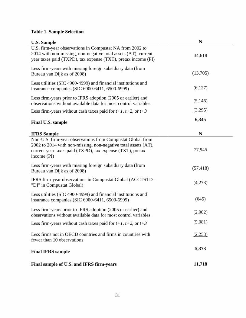
Our initial sample is comprised of U.S. firms from 2002-2014 with non-negative total
assets, cash taxes paid, tax expense, and pretax income (Table 1). We use subsidiary
information reported in Bureau van Dijk’s Orbis ownership database as of 2008 to compute
geographic scope and tax haven information.11 Orbis provides subsidiary information as of
a single point in time (i.e., when retrieved) so we assume the geographic scope (Num_ctry)
and tax haven presence (Txhaven) of sample firms in 2008 is applicable for earlier and later
years. We use the 2008 geographic data because we expect it best captures a firm’s
geographic presence around FIN 48.
We exclude observations related to firms in the utilities (SIC 4900-4999), financial,
and insurance industries (SIC 6000-6411, 6500-6999) because those firms are subject to
11 We compute geographic presence for U.S. firms using data from Bureau van Dijk rather than Exhibit 21 to maintain consistency with the IFRS sample. Subsidiary information for IFRS firms is only available through Bureau van Dijk.
14
statutory reporting requirements. To maintain a consistent sample, we then exclude
observations without three years of future taxes paid and observations without sufficient data
to compute our control variables. Finally, because we use IFRS firms as a benchmark sample,
we limit the sample period to years after mandatory IFRS adoption, or post-2005. A
limitation of this sample restriction is that it reduces our pre-FIN 48 period to a single year.
In robustness tests, we confirm that our inferences are robust to using pre-IFRS adoption
years.12 Our final U.S. sample consists of 6,345 firm-year observations spanning 2006-2012.
Table 1 tabulates our sample selection procedure.
[INSERT TABLE 1 HERE]
3.3 IFRS (control) sample
We obtain financial information for non-U.S. firms from Compustat Global. IFRS
firm-years are identified based on the accounting standard denoted in Compustat Global
(ACCSTD=”DI”).13 We also obtain subsidiary ownership data for IFRS firms from Bureau
van Dijk. To ensure our control sample have relatively similar macroeconomic conditions
and opportunities, we limit our primary analysis to firms domiciled in OECD countries. We
restrict the sample of countries in subsequent tests to those countries with institutional
similarities to the U.S, specifically we require firms to XXX. Imposing the same industry
and variable restrictions as in the U.S. sample yields a final sample of 5,373 IFRS firm-years
from 2006-2012 (Table 1). We also provide a breakdown of the sample by country and by
12 Our results remain unchanged when we extend the pre-FIN48 period to 2002 and when we redefine the pre-FIN 48 period as 2002-2004 (to bypass the IFRS transition year). However, our dataset contains relatively few non-U.S. observations with all variables defined before 2006. 13 The accounting standard code “DI” means that the domestic standards in use are generally in accordance with or fully compliant with IFRS. Alternatively, we classify IFRS firms based on the mandatory IFRS adoption dates for individual countries (Christensen, Hail, and Leuz 2013). Under this alternate classification, we assume that all firms domiciled in countries that mandatorily adopt IFRS are reporting under IFRS on their consolidated financial reports. The alternate classification method yields consistent inferences about the impact of FIN 48.
15
year in Table 2. Panel A shows that firms in Australia and the U.K. represent roughly 14%
and 27% of the IFRS firm-years, respectively. From Panel B, we see slightly more U.S. than
IFRS observations in each year, and the total number of observations slightly declined
following the financial crisis.
[INSERT TABLE 2 HERE]
3.4 Descriptive statistics
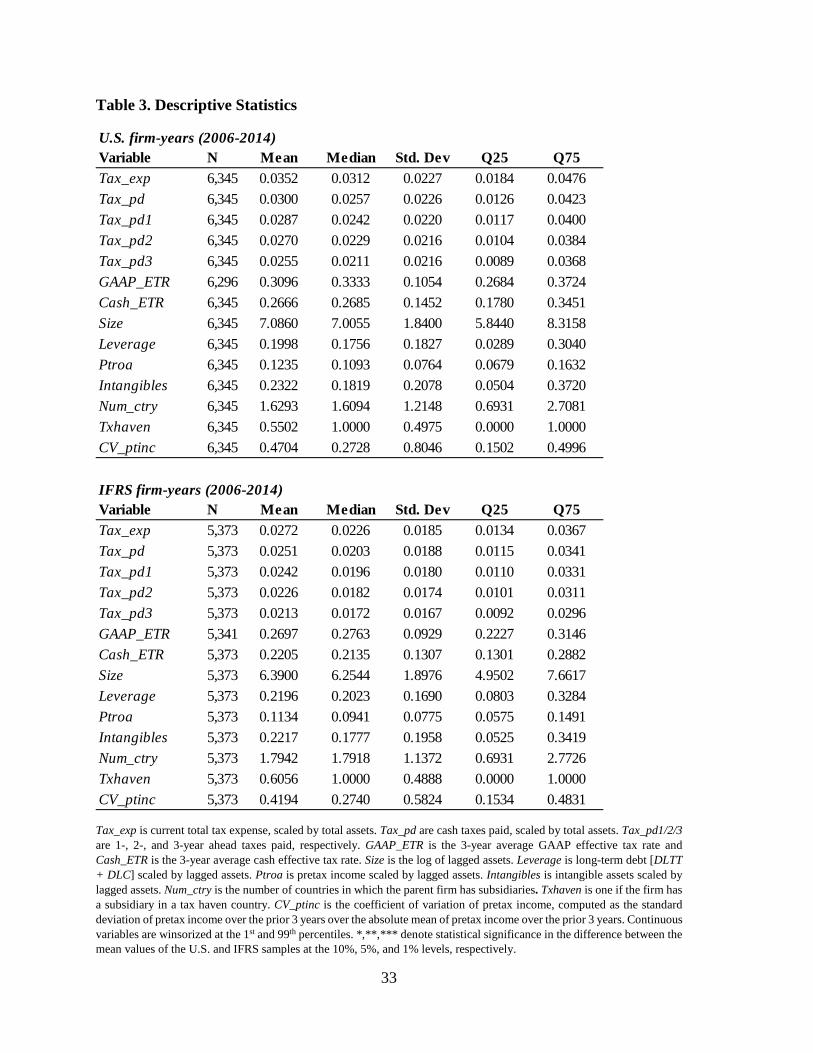
Table 3 displays descriptive statistics for the U.S. and the IFRS samples. The mean
U.S. and IFRS firms have a similar intangible intensity (23% for U.S., 22% for IFRS), tax
haven intensity (55% for U.S., 61% for IFRS), and geographic footprint (both have
subsidiaries in approximately 2 countries), which provides assurance that the samples are
comparable in terms of tax planning activities. On average, IFRS firms have lower GAAP
and cash ETRs than U.S. firms, consistent with many IFRS firms being located in lower-tax
jurisdictions. U.S. firms also tend to be larger and have more volatile pretax income than
IFRS firms.
[INSERT TABLE 3 HERE]
4. Results
4.1 Main test: Difference-in-differences
Table 4 presents our findings about the predictive ability of tax expense for future
cash taxes paid over 1-, 2-, and 3-year horizons. Panel A shows the relative association for
U.S. and IFRS firms, before and after FIN 48. In Panel B, we examine the predictive ability
of tax expense before and after FIN 48 separately for U.S. and IFRS firms.
16
In the pre-FIN 48 period, which we use as a baseline to identify the effect of FIN 48,
the predictive ability of tax expense for taxes paid is significantly lower for U.S. firms than
for IFRS firms across all forecast horizons (𝛽𝛽5). On average, tax expense is significantly
positively associated with future taxes paid for IFRS firms, and relatively less so for U.S.
firms. The difference in predictive ability between U.S. and IFRS firms grows as the horizon
increases. For U.S. firms, year t total tax expense is significantly less predictive of 2-year
ahead (t-stat = -2.428) and 3-year ahead (t-stat = -2.521) cash taxes paid than for IFRS firms.
For comparison, a dollar of total tax expense is associated with 30.6 cents of cash taxes,
scaled by assets, paid by IFRS firms in three years (𝛽𝛽1), and 18 cents of taxes (scaled) paid
by U.S. firms in three years (𝛽𝛽1+ 𝛽𝛽5), after controlling for current cash taxes paid.
Our empirical setting does not allow us to determine whether tax reserves are more
relevant under pre-FIN 48 U.S. GAAP than those measured under IFRS. Differences
between the relative predictive ability pre-FIN 48 can arise from cross-sectional differences
in tax planning, reporting choices, and innate firm characteristics, but this setting does not
allow us to identify these determinants empirically. The setting does, however, provide a
benchmark against which to test changes in the predictive ability post-FIN 48.
In the post-FIN 48 period, IFRS firms do not experience a significant change in the
predictive ability of tax expense for taxes paid in any of the next three years (𝛽𝛽6). U.S. firms,
in contrast, experience a significant relative improvement in the predictive ability of tax
expense for taxes paid in year t+3 (𝛽𝛽7 = 0.136, t-stat = 2.597). Moreover, the difference in
the total predictive ability of tax expense between U.S. and IFRS firms steadily shrinks as
the horizon increases. In fact, the ability of tax expense to predict 2- and 3-year ahead cash
taxes paid is no longer significantly different for U.S. and IFRS firms after FIN 48 (𝛽𝛽5+ 𝛽𝛽7=
17
0, F-stat = 1.77, 0.11, respectively). U.S. firms experience an insignificant change in the
predictive ability of tax expense for 1-year ahead taxes paid, relative to IFRS firms (t-stat =
-0.444). Total tax expense accrued by U.S. firms in the current period continues to be less
predictive of future taxes paid across all time horizons than that of IFRS firms.
These findings are consistent with FIN 48 increasing the convergence in accounting
for income taxes between U.S. and IFRS firms. The improvement over longer horizons is
consistent with improvements related to tax reserves given the three-year statute of
limitations for U.S. tax audits and the typical audit delays for large companies.
In Table 4, Panel B, we separately estimate the effect of FIN 48 on the predictive
ability of tax expense for the U.S. and IFRS samples. Doing so allows us to relax the
assumption that the effect of the control variables on future taxes paid are constant for both
subsamples. Partitioning the sample confirms that, for U.S. firms, total tax expense is
significantly more positively associated with t+3 taxes paid after FIN 48, which is consistent
with reserves unwinding over a longer horizon.
[INSERT TABLE 4 HERE]
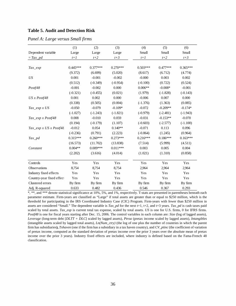
4.2 Audit and detection risk
To disentangle changes in tax positions because of the 100% audit assumption
required by FIN 48 and changes in measurement, we partition our sample based on firms’
likelihood of being audited by taxing authorities. First, because large firms are more likely
to be audited than small firms, we partition the U.S. and IFRS samples based on size. Large
firms are likely to be under greater audit scrutiny or even constant audit and therefore, are
less likely to have their reporting of tax expense affected by the assumption of 100% audit
18
risk introduced by FIN 48. In particular, firms that participate in the IRS’s Coordinated
Industry Case (CIC) program are large firms under continuous audit by the IRS. We identify
firms as large if they have assets of at least 250 million, which represents a lower bound
threshold for inclusion in the CIC program (Ayers, Seidman, and Towery 2016).
Table 5, Panel A, presents the results for the size-based subsamples. We find that our
main results are driven primarily by large firms, which experience relative improvements in
cash tax forecasts of t+3 taxes paid. In the small firm sample, the three-way interaction with
𝑃𝑃𝑃𝑃𝑃𝑃𝑃𝑃𝑃𝑃48 is insignificant, consistent with prior studies that do not identify an on-average
change in the relevance of tax expense post-FIN 48 (Robinson, Stomberg, and Towery 2016).
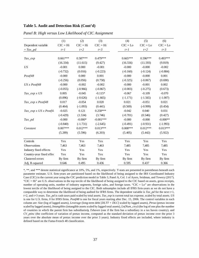
Next, we partition firms based on whether they have a high or low likelihood of being
audited by the IRS using the CIC program prediction model developed by Ayers, Seidman,
and Towery (2017) (specifically, the model in Table 3, Panel A, Col. 1 of Ayers et al.).
Following their methodology, we compute the likelihood of CIC program assignment based
on the following criteria identified in the Internal Revenue Manual: total assets, gross
receipts, number of operating entities, number of industries, total foreign sales, and foreign
taxes. In Table 5, Panel B, we partition the U.S. sample into firm-years in the top tercile of
likelihood of CIC assignment (“CIC = Hi”) and those in the lowest tercile of the likelihood
of CIC assignment (“CIC = Lo”). Because we do not have similar criteria to determine the
likelihood of audit by taxing authorities for IFRS firms, we include the entire sample of IFRS
firms for comparison with each subsample. As with the partition on size in Panel A, we find
that firms with a high likelihood of being audited (“CIC = Hi”) experience a strong positive
incremental association between tax expense and t+3 cash taxes paid. The tax expense of
firms with a low likelihood of CIC assignment (“CIC = Lo”) do not exhibit a significantly
19
different association with future taxes paid relative to the IFRS sample at any of the three
horizons.
[INSERT TABLE 5 HERE]
4.3 Current versus total tax expense
Prior to FIN 48, diverse practices and a lack of specific guidance led firms to classify
reserves for uncertain tax positions under both current and deferred tax expense (Gleason
2007, Blouin et al. 2010). Under FIN 48, firms are required to classify changes in tax reserves
as a current expense. We use total tax expense in our main tests to ensure that we capture all
tax reserves prior to FIN 48. Using total tax expense also mitigates concerns about
classification differences between IFRS and U.S. GAAP. Nevertheless, we also explore
whether current tax expense is differentially predictive of future taxes paid after FIN 48.
Because FIN 48 clarified the classification of tax reserves in addition to changing the
measurement of tax reserves, changes in the predictive power of current tax expense and
future tax cash flows would reflect both changes and provide additional evidence on the
impact of FIN 48 on the relevance of tax expense.
Table 6 provides the results of the association between future cash taxes paid and
both current and deferred tax expense. We observe a strong, positive association between
current tax expense and future cash taxes paid in t+2 and t+3, relative to IFRS firms and
relative to the pre-FIN 48 period, consistent with results for total tax expense. We find no
difference in the association between deferred tax expense and cash taxes paid for U.S. and
IFRS firms after FIN 48. Improvements in the predictive ability of tax expense for tax cash
flows are attributable to the impact of FIN 48 on current tax expense.
[INSERT TABLE 6 HERE]
20
4.4 Early versus late FIN 48 adoption period
To investigate whether the beneficial effects of FIN 48 reverse over time, we examine
whether the predictive ability of tax expense changed from early in the adoption period
(2007-2010) to late in the adoption period (2011-2014). If the cash-accrual mapping reverts
to pre-FIN 48 levels, we would expect no difference in the predictive ability of tax expense
from pre-FIN 48 in the later period. In contrast, we find that the incremental predictive ability
is actually stronger for t+2 and t+3 cash taxes paid in the later period. The results are more
consistent with continuing improvements in the mapping following better or more complete
implementation later in the FIN 48 period and after the financial crisis. We cannot rule out
the possibility that the tax cash-accrual mapping diminished for IFRS firms during the later
period.
[INSERT TABLE 7 HERE]
4.5 Subsamples of IFRS countries
To provide assurance that idiosyncratic country-level institutional features among our
control sample of OECD countries are not driving our results, we reduce the control sample
to the two countries most similar to the U.S. in terms of institutional development, the U.K.
and Australia. If country-level differences are affecting our main results, estimation on this
restricted sample should yield different results from those reported in Table 4, Panel A.
Results are reported in Table 7 and are consistent with those using the full control sample:
under U.S. GAAP, the ability of tax expense to predict cash taxes paid three years in the
future improved after FIN 48.
[INSERT TABLE 8 HERE]
21
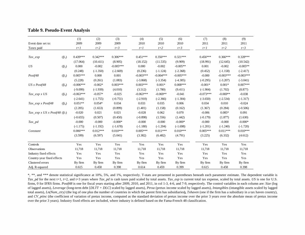
4.6 Pseudo-event analysis
Although we control for current cash taxes paid in our regressions, it is possible that
systematic patterns in the cash-accrual relation in U.S. firms contribute to our finding of an
incremental improvement. To mitigate these concerns, we perform a pseudo-event analysis
in which we redefine the FIN 48 adoption year as 2009, 2010, and 2011. If our findings are
attributable to changes brought about by FIN 48, we would not expect to find significant
results when we alter the event year. In Table 8, we see no significant incremental
improvement for U.S. firms after FIN 48 when we set alternate event years, with the minor
exception of 2011. When we set the event year to 2011, tax expense are incrementally more
predictive of t+2 cash taxes paid for U.S. firms, albeit marginally so (t-stat = 1.877).
Altogether, the results suggest that FIN 48 had a meaningful impact on the predictive ability
of tax reserves.
[INSERT TABLE 9 HERE]
5. Robustness tests
5.1 Extended pre-FIN 48 period
Because IFRS became mandatory for firms in most adopting countries starting Dec.
31, 2005 and FIN 48 was effective for U.S. firms starting Dec. 15, 2006, we have just one
year of data in the pre-FIN 48 period. In untabulated tests, we extend the pre-FIN 48 period
to 2002, prior to mandatory IFRS adoption. Although our inferences remain unchanged, we
were able to collect very few observations (fewer than 100) before 2005, perhaps because
firms did not consistently report (or the data aggregator did not consistently collect) financial
reports on local GAAP. Because lengthening the pre-FIN 48 period adds noise and does not
allow us to maintain our assumptions about non-GAAP accounting for income taxes (many
22
of the firms in IFRS countries reported on local GAAP prior to 2005), we continue to use
only IFRS firm-years in the pre period for our reported results.
5.2 Change in accounting for stock options
An additional time period concern is that SFAS 123R, which changed the recognition
of stock-based compensation expense related to options for fiscal years beginning on or after
June 15, 2005, confounds the effect of FIN 48. SFAS 123R mandated recognition of stock-
based compensation expense, thereby strengthening the mapping between tax expense and
future cash taxes. To address this concern, we redefine tax expense (Tax_exp) to adjust for
the tax effect of stock-based compensation for U.S. firms (Tax_exp – Comp_exp*35%, where
inferences are unchanged, suggesting that the change in accounting for stock-based
compensation expense due to SFAS 123R is not responsible for changes in the predictive
ability of tax expense after FIN 48.
5.3 Global financial crisis
Another challenge facing early studies of the effect of FIN 48 is that a portion of the
post period coincides with the global financial crisis. When we drop the financial crisis years
entirely, our main results are even stronger; in addition, tax expense becomes incrementally
predictive of t+2 taxes paid when we remove observations from 2008 and 2009 (t-stat =
2.102). Results are also robust to dropping 2007 as the FIN 48 transitional year. Additionally,
when we limit the post period to the crisis period, 2008-2009, we find weaker but still
statistically significant results for the incremental predictive ability of U.S. tax expense for
t+3 taxes paid. We conclude that our results are not driven by a single time period.
23
5.4 Sensitivity to sample composition
Our results remain unchanged (and even stronger) when we require firms to have at
least one year in both the pre- and post-FIN 48 periods (although doing so shrinks our sample
by 30%), providing comfort that our results are not sensitive to changes in the sample
composition over time. Finally, we test whether firms for which tax expense is unlikely
reflect the effect of FIN 48 affect our results by dropping firms which have either not reported
UTBs or have reported zero UTBs during the entire post-FIN 48 sample period. Results are
again robust and, as expected, we find that the improvement is concentrated only among
firms that have reported UTBs.
6. Conclusion
We examine the relation between tax expense and cash taxes paid one, two and three
years later to determine whether FIN 48 affected the predictive ability of tax expense. We
find the tax expense-cash relation is weaker for U.S. firms relative to IFRS firms pre-FIN 48.
After FIN 48, tax expense for U.S. firms better predicts cash taxes paid in the third year.
Additionally, the difference in predictive ability relative to IFRS firms disappears over the
three-year horizon, consistent with FIN 48 improving the relevance of accounting for
uncertain tax benefits. While we find that tax expense is more predictive of future taxes paid
after FIN 48, we cannot rule out the possibility that the improvement results from increased
auditor attention following the standard change rather than a change in measurement. We
leave distinguishing between these two potential forecasts to future work.
While our results suggest FIN 48 improved accounting for tax reserves for U.S. firms,
differences between U.S. and IFRS accounting for tax reserves persist. U.S. firms are
required to disclose significantly more information about tax reserves in financial statements
24
while IFRS firms are able to consider the probability of audit and detection by tax authorities
in estimating tax reserves. Critics of FIN 48 argue the inability to consider audit and detection
probabilities results in systematic over-estimation of reserves. Our results suggest that U.S.
accounting for tax reserves for small firms with low probabilities of audit and detection
continues to be less relevant than that for IFRS firms. In contrast, the relevance of tax
reserves increased for large U.S. firms with higher probabilities of audit and detection.
Recently, the IASB adopted measurement standards similar to FIN 48 to account for tax
uncertainties, including a prohibition on incorporating the probability of audit and detection
in tax reserve estimates. Our results suggest this is unlikely to improve the relevance of tax
reserves for firms with lower probabilities of audit and detection.
25
References
Austin, Chelsea R. 2014. “Analysis of differences in the recognized and realized costs of stock options and the implications for studies of tax avoidance.” Dissertation, The University of Iowa.
Ayers, Benjamin C., Jeri K. Seidman, and Erin Towery. 2017. “Taxpayer Behavior under Audit Certainty.” Contemporary Accounting Research (forthcoming).
Blouin, Jennifer L., Cristi A. Gleason, Lillian F. Mills, and Stephanie A. Sikes. 2010. “Pre-Empting Disclosure? Firms’ Decisions Prior to FIN No. 48.” The Accounting Review 85 (3): 791–815. doi:10.2308/accr.200.85.3.791.
Blouin, Jennifer, and Irem Tuna. 2007. “Tax Contingencies: Cushioning the Blow to Earnings?” NBER Financial Reporting and Taxation Conference, April. http://citeseerx.ist.psu.edu/viewdoc/download?doi=10.1.1.169.2476&rep=rep1&type=pdf.
Bratten, B., Gleason, C.A., Larocque, S.A. and Mills, L.F., 2016. Forecasting taxes: New evidence from analysts. The Accounting Review, 92(3), pp.1-29.
Cazier, Richard, Sonja Rego, Xiaoli Tian, and Ryan Wilson. 2014. “The Impact of Increased Disclosure Requirements and the Standardization of Accounting Practices on Earnings Management through the Reserve for Income Taxes.” Review of Accounting Studies 20 (1): 436–69. doi:10.1007/s11142-014-9302-y.
Christensen, Hans B., Luzi Hail, and Christian Leuz. 2013. “Mandatory IFRS Reporting and Changes in Enforcement.” Journal of Accounting and Economics, Conference Issue on Accounting Research on Classic and Contemporary IssuesUniversity of Rochester, Simon Business School, 56 (2–3, Supplement 1): 147–77. doi:10.1016/j.jacceco.2013.10.007.
Ciconte, Will, Michael P. Donohoe, Petro Lisowsky, and Michael A. Mayberry. 2016. “Predictable Uncertainty: The Relation between Unrecognized Tax Benefits and Future Income Tax Cash Outflows.” SSRN Scholarly Paper ID 2390150. Rochester, NY: Social Science Research Network. http://papers.ssrn.com/abstract=2390150.
De Simone, Lisa, John R. Robinson, and Bridget Stomberg. 2013. “Distilling the Reserve for Uncertain Tax Positions: The Revealing Case of Black Liquor.” Review of Accounting Studies 19 (1): 456–72. doi:10.1007/s11142-013-9257-4.Dyreng, S.D., Hanlon, M., Maydew, E.L. and Thornock, J.R., 2017. Changes in corporate effective tax rates over the past 25 years. Journal of Financial Economics, 124(3), pp.441-463.
Edwards, A., Schwab, C. and Shevlin, T., 2015. Financial constraints and cash tax savings. The Accounting Review, 91(3), pp.859-881.
Gleason, Cristi A. 2007. "An Early Look at FIN 48 Disclosures." Accounting Policy and Practice Special Report Volume 3, Number 6: BNA Tax and Accounting.
Gleason, Cristi A, and Lillian F Mills. 2002. “Materiality and Contingent Tax Liability Reporting.” The Accounting Review 77 (2): 317–42.
Gleason, Cristi A., Lillian F. Mills, and Michelle L. Nessa. 2017. “Does FIN 48 Improve Firms’ Estimates of Tax Reserves?” Contemporary Accounting Research, no. forthcoming. https://papers.ssrn.com/abstract=2594507.
Goldman, Nathan C. 2017. "Does Disclosure Quantity Affect Investment Efficiency?" University of Texas at Dallas working paper.
26
Gupta, Sanjay, Rick C. Laux, and Daniel P. Lynch. 2016. “Do Firms Use Tax Reserves to Meet Analysts’ Forecasts? Evidence from the Pre- and Post-FIN 48 Periods.” Contemporary Accounting Research 33 (3): 1044–74. doi:10.1111/1911-3846.12180.
Hainmueller, Jens. 2012. "Entropy balancing for causal effects: A multivariate reweighting method to produce balanced samples in observational studies." Political Analysis 20.1: 25-46.
Hainmueller, Jens, and Yiqing Xu. 2013. "ebalance: A Stata Package for Entropy Balancing." Journal of Statistical Software 54 (7).
Kim, Myungsun, and William Kross. 2005. “The Ability of Earnings to Predict Future Operating Cash Flows Has Been Increasing—Not Decreasing.” Journal of Accounting Research 43 (5): 753–80. doi:10.1111/j.1475-679X.2005.00189.x.
Law, K.K. and Mills, L.F., 2015. Taxes and financial constraints: Evidence from linguistic cues. Journal of Accounting Research, 53(4), pp.777-819.
Lisowsky, Petro, Leslie Robinson, and Andrew Schmidt. 2013. “Do Publicly Disclosed Tax Reserves Tell Us About Privately Disclosed Tax Shelter Activity?” Journal of Accounting Research 51 (3): 583–629. doi:10.1111/joar.12003.
“Post-Implementation Review of FIN 48.” 2012. The Tax Adviser. May 1. http://www.thetaxadviser.com/issues/2012/may/clinic-story-13.html.
Robinson, Leslie A., Bridget Stomberg, and Erin M. Towery. 2015. “One Size Does Not Fit All: How the Uniform Rules of FIN 48 Affect the Relevance of Income Tax Accounting.” The Accounting Review 91 (4): 1195–1217. doi:10.2308/accr-51263.
Tysiac, Ken. 2012. “FAF Releases ‘post-Implementation Review’ of FIN 48.” Journal of Accountancy. January 12. http://www.journalofaccountancy.com/news/2012/jan/20124992.html.
27
Appendix A: Variable Definitions
Variables Description (Compustat variables shown in brackets) Variables of interest 𝑇𝑇𝑇𝑇𝑇𝑇_𝑝𝑝𝑝𝑝 Cash taxes paid [TXPD], scaled by total assets [AT] over the next 1, 2,
and 3 years
𝑇𝑇𝑇𝑇𝑇𝑇_𝑒𝑒𝑇𝑇𝑝𝑝 Total tax expense [TXT], scaled by total assets [AT]
𝑈𝑈𝑆𝑆 =1 if the firm is domiciled in the U.S.; 0 if the firm is domiciled outside of the U.S. and reports under IFRS. IFRS firm-years are identified based on the accounting standard “DI” in Compustat Global. “DI” means that the domestic standards used are in accordance with or fully compliant with IFRS.
𝑃𝑃𝑃𝑃𝑃𝑃𝑃𝑃𝑃𝑃48 =1 for fiscal years starting after December 15, 2006; 0 otherwise
Controls and other 𝑆𝑆𝑆𝑆𝑆𝑆𝑒𝑒 Log of lagged total assets [AT]
𝐿𝐿𝑒𝑒𝐿𝐿𝑒𝑒𝐶𝐶𝑇𝑇𝐿𝐿𝑒𝑒 The sum of long-term debt [DLTT] and the current maturity of long-
term debt [DLC], scaled by lagged total assets [AT]
𝑃𝑃𝑃𝑃𝐶𝐶𝑃𝑃𝑇𝑇 Pretax income [PI], scaled by lagged total assets [AT]
𝐼𝐼𝐶𝐶𝑃𝑃𝑇𝑇𝐶𝐶𝐿𝐿𝑆𝑆𝐼𝐼𝐶𝐶𝑒𝑒𝑃𝑃 Intangible assets [INTAN], scaled by lagged total assets [AT]
𝑁𝑁𝑁𝑁𝑁𝑁_𝑐𝑐𝑃𝑃𝐶𝐶𝑐𝑐 The number of countries in which the parent firm has subsidiaries. The number of countries is based on subsidiary ownership data from Bureau van Dijk as of 2008 (applied to all years)
𝑇𝑇𝑇𝑇ℎ𝑇𝑇𝐿𝐿𝑒𝑒𝐶𝐶 =1 if the firm has a subsidiary in a tax haven country as defined by the OECD list of tax havens. Whether a subsidiary is in a tax haven is based on ownership data from Bureau van Dijk as of 2008 (applied to all years)
𝐶𝐶𝐶𝐶_𝑝𝑝𝑃𝑃𝑆𝑆𝐶𝐶𝑐𝑐 The coefficient of variation of pretax income, computed as the standard deviation of annual pretax income [PI] over the prior 3 years over the absolute mean of pretax income over the prior 3 years
28
Appendix B: Summary of Differences in Accounting for Income Taxes between U.S. GAAP and IFRS
This table summarizes differences in accounting for income taxes between U.S. GAAP and IFRS as of 2015 (adapted and compiled from Deloitte 2017, Ernst and Young 2013, PricewaterhouseCoopers LLP 2016, IAS 12). In general, under U.S. GAAP, accounting for income taxes is governed by ASC 740, which includes the provisions of FIN 48 (ASC 740-10). Under IFRS, accounting for income taxes is governed by IAS 12.
Topic U.S. GAAP IFRS Tax basis Tax basis is defined by law. Tax basis is determined based on
what is deductible for tax purposes, and is influenced by the way the entity intends to settle or recover the carrying amount (by sale or through use).
Tax rates Enacted tax rates are used. Enacted or “substantively enacted” tax rates are used, where “substantively enacted” means only perfunctory actions are required for the measure to become law.
Recognition of deferred tax assets
Deferred tax assets are recognized in full and reduced by a valuation allowance for the amount of the asset that is not more likely than not (greater than 50% likely) to be recognized.
Unrecognized deferred tax assets are only recognized if it is “probable” (or “more likely than not”) they will be utilized (IAS 12, par. 37). No valuation allowance account is used.
Uncertain tax positions
ASC 740-10 (FIN 48) establishes a 2-step recognition and measurement approach. A benefit is recognized if it is more likely than not that the underlying tax position will be upheld based on its technical merits. The benefit is measured as the greatest amount that is more likely than not to being realized upon settlement.
IAS 12 does not provide formal guidance addressing the accounting for tax uncertainties. The guidance in IAS 37 is relevant because an uncertain tax position may generate a liability of uncertain timing and amount. Recognition and measurement is based on the best estimate of the amount expected to be paid. If it is more likely than not that a liability has been incurred, it is often measured using either a single-best-estimate or a weighted average probability of the outcomes.
Foreign nonmonetary assets and liabilities remeasured from local currency to functional currency
No deferred tax is recognized on the remeasurement of foreign nonmonetary assets and liabilities from local currency to functional currency.
Deferred tax is recognized on the difference between the carrying value based on historical exchange rate from the local to functional currency and the current tax basis based on current exchange rates.
Reconciliation of actual and expected tax rate
Required for public companies only. Expected tax expense is computed by
Required for all entities applying IFRSs. Expected tax expense is
29
applying the federal statutory rate to pretax income from continuing operations. Non-public companies must disclose the reconciling items but not the amounts.
computed by applying the applicable tax rate(s) to accounting income. The basis on which applicable tax rate is computed is disclosed.
Special deductions (tax benefits for specific jurisdictions or circumstances)
Special deduction tax benefits should be recognized in the year in which they are available to reduce taxable income on the tax returns. They should not be anticipated by offsetting a deferred tax liability.
No similar guidance in IAS 12.
Undistributed earnings of investees
Deferred tax is recognized on undistributed earnings of domestic subsidiaries and joint ventures. Deferred tax is also recognized on undistributed earnings of foreign subsidiaries and joint ventures, except that which are considered permanently reinvested.
Deferred tax is recognized on the undistributed earnings of any investee unless: (1) the parent has control over timing of the reversal of the temporary differences; and (2) it is more likely than not that the temporary difference will not reverse in the foreseeable future.
Share-based compensation
Deferred tax is computed on the same basis as the share-based compensation expense recognized.
Deferred tax is computed on the basis of the hypothetical tax deduction for the share-based payment in every period.
Intercompany sales Tax expense from intercompany sales is deferred until the related asset is disposed of, and no deferred taxes are recognized for the purchaser's change in tax basis.
Tax expense from intercompany sales is recognized immediately, and the buyer's tax rate is used to recognize deferred taxes for the change in tax basis.
Balance sheet classification
The classification of deferred tax assets and liabilities as current or noncurrent depends on the classification of the underlying that generated the temporary difference.
All deferred tax assets and liabilities are classified as noncurrent.
Subsequent changes in deferred taxes that were originally charged or credited to equity (backward tracing)
Subsequent changes to deferred taxes originally charged or credited to equity are generally allocated to continuing operations, not to equity.
Subsequent changes to deferred taxes originally charged or credited to equity are also charged or credited directly back to equity.
Other exceptions to the general principle that deferred tax is recognized for all temporary differences
Leveraged lease exemption: no deferred tax is recognized on leveraged leases (see ASC 840-30)
"Initial recognition" exemption: no deferred tax is recognized for temporary differences from the initial recognition of an asset or liability that (a) does not arise from a business combination and (b) does not affect accounting or taxable income at the time of the transaction (IAS 12, par. 24).
30
Appendix C. Accounting for Uncertain Tax Positions under U.S. GAAP and IFRS
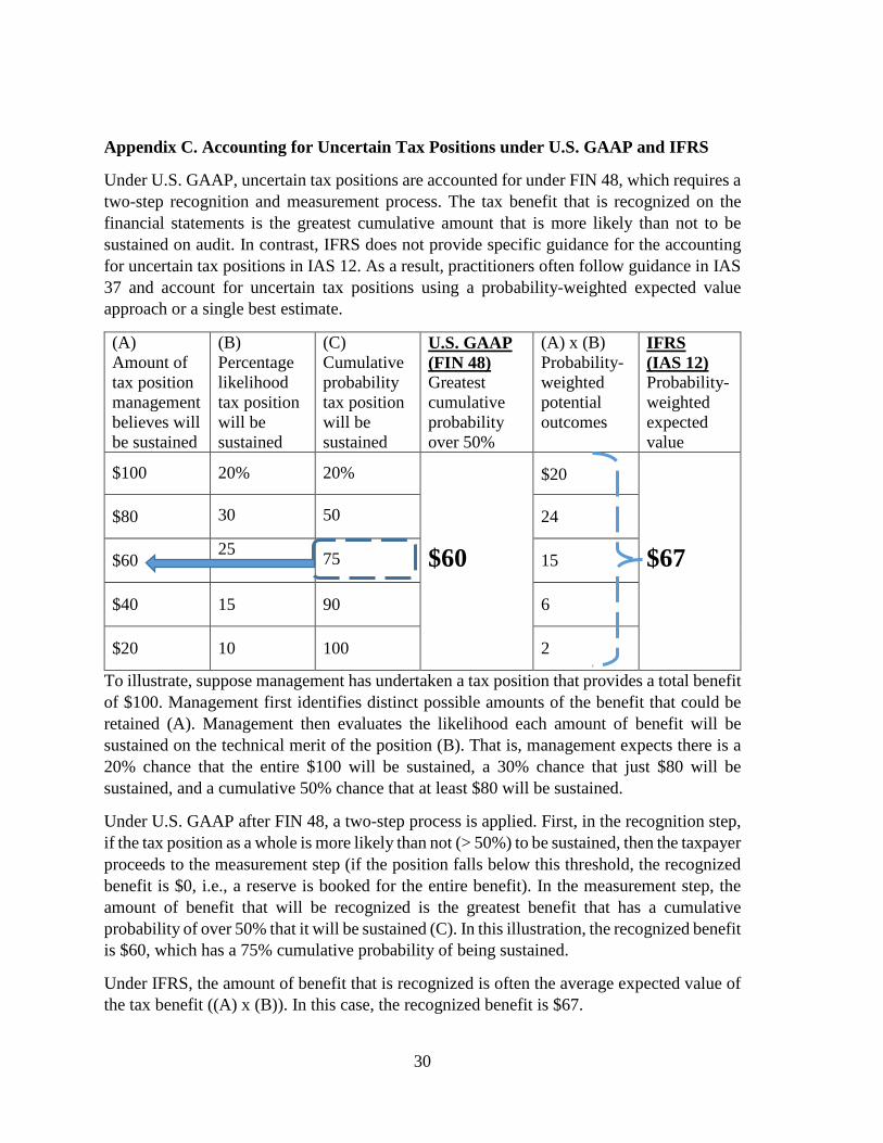
Under U.S. GAAP, uncertain tax positions are accounted for under FIN 48, which requires a two-step recognition and measurement process. The tax benefit that is recognized on the financial statements is the greatest cumulative amount that is more likely than not to be sustained on audit. In contrast, IFRS does not provide specific guidance for the accounting for uncertain tax positions in IAS 12. As a result, practitioners often follow guidance in IAS 37 and account for uncertain tax positions using a probability-weighted expected value approach or a single best estimate.
(A) Amount of tax position management believes will be sustained
(B) Percentage likelihood tax position will be sustained
(C) Cumulative probability tax position will be sustained
U.S. GAAP (FIN 48) Greatest cumulative probability over 50%
(A) x (B) Probability-weighted potential outcomes
IFRS (IAS 12) Probability-weighted expected value
$100
20%
20% $60
$20 $67
$80
30
50
24
$60
25
75
15
$40
15
90
6
$20
10
100
2
To illustrate, suppose management has undertaken a tax position that provides a total benefit of $100. Management first identifies distinct possible amounts of the benefit that could be retained (A). Management then evaluates the likelihood each amount of benefit will be sustained on the technical merit of the position (B). That is, management expects there is a 20% chance that the entire $100 will be sustained, a 30% chance that just $80 will be sustained, and a cumulative 50% chance that at least $80 will be sustained.
Under U.S. GAAP after FIN 48, a two-step process is applied. First, in the recognition step, if the tax position as a whole is more likely than not (> 50%) to be sustained, then the taxpayer proceeds to the measurement step (if the position falls below this threshold, the recognized benefit is $0, i.e., a reserve is booked for the entire benefit). In the measurement step, the amount of benefit that will be recognized is the greatest benefit that has a cumulative probability of over 50% that it will be sustained (C). In this illustration, the recognized benefit is $60, which has a 75% cumulative probability of being sustained.
Under IFRS, the amount of benefit that is recognized is often the average expected value of the tax benefit ((A) x (B)). In this case, the recognized benefit is $67.
31
Table 1. Sample Selection
U.S. Sample N U.S. firm-year observations in Compustat NA from 2002 to 2014 with non-missing, non-negative total assets (AT), current year taxes paid (TXPD), tax expense (TXT), pretax income (PI)
34,618
Less firm-years with missing foreign subsidiary data (from Bureau van Dijk as of 2008)
(13,705)
Less utilities (SIC 4900-4999) and financial institutions and insurance companies (SIC 6000-6411, 6500-6999)
(6,127)
Less firm-years prior to IFRS adoption (2005 or earlier) and observations without available data for most control variables
(5,146)
Less firm-years without cash taxes paid for t+1, t+2, or t+3 (3,295) Final U.S. sample
6,345
IFRS Sample N Non-U.S. firm-year observations from Compustat Global from 2002 to 2014 with non-missing, non-negative total assets (AT), current year taxes paid (TXPD), tax expense (TXT), pretax income (PI)
77,945
Less firm-years with missing foreign subsidiary data (from Bureau van Dijk as of 2008) (57,418)
IFRS firm-year observations in Compustat Global (ACCTSTD = "DI" in Compustat Global)
(4,273)
Less utilities (SIC 4900-4999) and financial institutions and insurance companies (SIC 6000-6411, 6500-6999)
(645)
Less firm-years prior to IFRS adoption (2005 or earlier) and observations without available data for most control variables
(2,902)
Less firm-years without cash taxes paid for t+1, t+2, or t+3 (5,081) Less firms not in OECD countries and firms in countries with fewer than 10 observations
(2,253)
Final IFRS sample 5,373
Final sample of U.S. and IFRS firm-years 11,718
32
Table 2. Sample Composition
Panel A: Observations by Country
Panel B: U.S. and IFRS obs. by Year
Country # Obs. Country # Obs.1 Australia 768 13 Ireland 63 2 Austria 88 14 Israel 34 3 Belgium 76 15 Italy 84 4 Switzerland 330 16 Netherlands 170 5 Chile 15 17 Norway 112 6 Germany 454 18 New Zealand 135 7 Denmark 119 19 Poland 144 8 Spain 118 20 Portugal 27 9 Finland 219 21 Slovenia 21
10 France 398 22 Sweden 366 11 United Kingdom 1,462 23 Turkey 64 12 Greece 106 24 United States 6,345
11,718
Year U.S. IFRS Total Obs.2006 1,124 755 1,879 2007 1,085 943 2,028 2008 885 859 1,744 2009 770 721 1,491 2010 767 770 1,537 2011 881 771 1,652 2012 833 554 1,387 Total 6,345 5,373 11,718
33
Table 3. Descriptive Statistics
Tax_exp is current total tax expense, scaled by total assets. Tax_pd are cash taxes paid, scaled by total assets. Tax_pd1/2/3 are 1-, 2-, and 3-year ahead taxes paid, respectively. GAAP_ETR is the 3-year average GAAP effective tax rate and Cash_ETR is the 3-year average cash effective tax rate. Size is the log of lagged assets. Leverage is long-term debt [DLTT + DLC] scaled by lagged assets. Ptroa is pretax income scaled by lagged assets. Intangibles is intangible assets scaled by lagged assets. Num_ctry is the number of countries in which the parent firm has subsidiaries. Txhaven is one if the firm has a subsidiary in a tax haven country. CV_ptinc is the coefficient of variation of pretax income, computed as the standard deviation of pretax income over the prior 3 years over the absolute mean of pretax income over the prior 3 years. Continuous variables are winsorized at the 1st and 99th percentiles. *,**,*** denote statistical significance in the difference between the mean values of the U.S. and IFRS samples at the 10%, 5%, and 1% levels, respectively.
F -test: β5+β7=0 17.81*** 1.77 0.11p = 0.000 p = 0.1838 p = 0.7383
Observations 11,718 11,718 11,718 11,718 11,718 11,718Industry fixed effects Yes Yes Yes Yes Yes YesCountry-year fixed effects Yes Yes Yes Yes Yes YesClustered errors By firm By firm By firm By firm By firm By firmAdj. R-squared 0.577 0.614 0.429 0.457 0.368 0.400
35
Table 4. Predictive Ability of Tax Expense for Taxes Paid in t+1, t+2, and t+3 (Cont’d)
Panel B: U.S. versus IFRS
*, **, and *** denote statistical significance at 10%, 5%, and 1%, respectively. T-stats are presented in parentheses beneath each parameter estimate. The dependent variable is Tax_pd for the next t+1, t+2, and t+3 years. Tax_pd is cash taxes paid scaled by total assets. Tax_exp is current total tax expense, scaled by total assets. US is one for U.S. firms, 0 for IFRS firms. Postf48 is one for fiscal years starting after Dec. 15, 2006. Size is the log of lagged assets. Leverage is long-term debt [DLTT + DLC] scaled by lagged assets. Ptroa is pretax income scaled by lagged assets. Intangibles is intangible assets scaled by lagged assets. Ln(Num_ctry) is the log of one plus the number of countries in which the parent firm has subsidiaries. Txhaven is one if the firm has a subsidiary in a tax haven country. CV_ptinc is the coefficient of variation of pretax income, computed as the standard deviation of pretax income over the prior 3 years over the absolute mean of pretax income over the prior 3 years. Industry fixed effects are included, where industry is defined based on the Fama-French 48 classification.
(1) (2) (3) (4) (5) (6)Dependent variable US IFRS US IFRS US IFRS= Tax_pd t+1 t+1 t+2 t+2 t+3 t+3
Observations 6,345 5,373 6,345 5,373 6,345 5,373Industry fixed effects Yes Yes Yes Yes Yes YesCountry-year fixed effect Yes Yes Yes Yes Yes YesClustered errors By firm By firm By firm By firm By firm By firmAdj. R-squared 0.555 0.696 0.411 0.526 0.373 0.448
36
Table 5. Audit and Detection Risk
Panel A: Large versus Small firms
*, **, and *** denote statistical significance at 10%, 5%, and 1%, respectively. T-stats are presented in parentheses beneath each parameter estimate. Firm-years are classified as “Large” if total assets are greater than or equal to $250 million, which is the threshold for participating in the IRS Coordinated Industry Case (CIC) Program. Firm-years with fewer than $250 million in assets are considered “Small.” The dependent variable is Tax_pd for the next t+1, t+2, and t+3 years. Tax_pd is cash taxes paid scaled by total assets. Tax_exp is current total tax expense, scaled by total assets. US is one for U.S. firms, 0 for IFRS firms. Postf48 is one for fiscal years starting after Dec. 15, 2006. The control variables in each column are: Size (log of lagged assets), Leverage (long-term debt [DLTT + DLC] scaled by lagged assets), Ptroa (pretax income scaled by lagged assets), Intangibles (intangible assets scaled by lagged total assets), Ln(Num_ctry) (the log of one plus the number of countries in which the parent firm has subsidiaries), Txhaven (one if the firm has a subsidiary in a tax haven country), and CV_ptinc (the coefficient of variation of pretax income, computed as the standard deviation of pretax income over the prior 3 years over the absolute mean of pretax income over the prior 3 years). Industry fixed effects are included, where industry is defined based on the Fama-French 48 classification.
(1) (2) (3) (4) (5) (6)Dependent variable Large Large Large Small Small Small= Tax_pd t+1 t+2 t+3 t+1 t+2 t+3
Controls Yes Yes Yes Yes Yes YesObservations 8,754 8,754 8,754 2,964 2,964 2,964Industry fixed effects Yes Yes Yes Yes Yes YesCountry-year fixed effect Yes Yes Yes Yes Yes YesClustered errors By firm By firm By firm By firm By firm By firmAdj. R-squared 0.633 0.482 0.436 0.546 0.367 0.293
37
Table 5. Audit and Detection Risk (Cont’d)
Panel B: High versus Low Likelihood of CIC Assignment
*, **, and *** denote statistical significance at 10%, 5%, and 1%, respectively. T-stats are presented in parentheses beneath each parameter estimate. U.S. firm-years are partitioned based on the likelihood of being assigned to the IRS Coordinated Industry Case (CIC) in the current year using the CIC prediction model in Table 3, Panel A, Col. 1 of Ayers, Seidman, and Towery (2017). “CIC = Hi” are U.S. observations in the top tercile of the likelihood of being assigned to the CIC based on assets, gross receipts, number of operating units, number of industry segments, foreign sales, and foreign taxes. “CIC = Lo” are observations in the lowest tercile of the likelihood of being assigned to the CIC. Both subsamples include all IFRS firm-years as we do not have a comparable way to determine the likelihood of being audited for IFRS firms. The dependent variable is Tax_pd for the next t+1, t+2, and t+3 years. Tax_pd is cash taxes paid scaled by total assets. Tax_exp is current total tax expense, scaled by total assets. US is one for U.S. firms, 0 for IFRS firms. Postf48 is one for fiscal years starting after Dec. 15, 2006. The control variables in each column are: Size (log of lagged assets), Leverage (long-term debt [DLTT + DLC] scaled by lagged assets), Ptroa (pretax income scaled by lagged assets), Intangibles (intangible assets scaled by lagged total assets), Ln(Num_ctry) (the log of one plus the number of countries in which the parent firm has subsidiaries), Txhaven (one if the firm has a subsidiary in a tax haven country), and CV_ptinc (the coefficient of variation of pretax income, computed as the standard deviation of pretax income over the prior 3 years over the absolute mean of pretax income over the prior 3 years). Industry fixed effects are included, where industry is defined based on the Fama-French 48 classification.
(1) (2) (3) (4) (5) (6)Dependent variable CIC = Hi CIC = Hi CIC = Hi CIC = Lo CIC = Lo CIC = Lo= Tax_pd t+1 t+2 t+3 t+1 t+2 t+3
Controls Yes Yes Yes Yes Yes YesObservations 7,463 7,463 7,463 7,485 7,485 7,485Industry fixed effects Yes Yes Yes Yes Yes YesCountry-year fixed effec Yes Yes Yes Yes Yes YesClustered errors By firm By firm By firm By firm By firm By firmAdj. R-squared 0.646 0.495 0.436 0.595 0.437 0.366
38
Table 6. Current versus Deferred Tax Expense
*, **, and *** denote statistical significance at 10%, 5%, and 1%, respectively. T-stats are presented in parentheses beneath each parameter estimate. The dependent variable is Tax_pd for the next t+1, t+2, and t+3 years where Tax_pd is cash taxes paid scaled by total assets. Tax_exp is defined as current or deferred tax expense, scaled by total assets, where current tax expense is [TXC] and deferred is [TXDI]. US is one for U.S. firms, 0 for IFRS firms. Postf48 is one for fiscal years starting after Dec. 15, 2006. The control variables in each column are: Size (log of lagged assets), Leverage (long-term debt [DLTT + DLC] scaled by lagged assets), Ptroa (pretax income scaled by lagged assets), Intangibles (intangible assets scaled by lagged total assets), Ln(Num_ctry) (the log of one plus the number of countries in which the parent firm has subsidiaries), Txhaven (one if the firm has a subsidiary in a tax haven country), and CV_ptinc (the coefficient of variation of pretax income, computed as the standard deviation of pretax income over the prior 3 years over the absolute mean of pretax income over the prior 3 years). Industry fixed effects are included, where industry is defined based on the Fama-French 48 classification.
(1) (2) (3) (4) (5) (6)Tax_exp = Current Deferred Current Deferred Current Deferred
Controls Yes Yes Yes Yes Yes YesObservations 6,821 6,813 6,821 6,813 6,821 6,813Industry fixed effects Yes Yes Yes Yes Yes YesCountry-year fixed effects Yes Yes Yes Yes Yes YesClustered errors By firm By firm By firm By firm By firm By firmAdj. R-squared 0.608 0.591 0.453 0.440 0.397 0.385
39
Table 7. Early versus Late FIN 48 Adoption Period
*, **, and *** denote statistical significance at 10%, 5%, and 1%, respectively. T-stats are presented in parentheses beneath each parameter estimate. The dependent variable is Tax_pd for the next t+1, t+2, and t+3 years where Tax_pd is cash taxes paid scaled by total assets. Tax_exp is defined as current total tax expense, scaled by total assets. US is one for U.S. firms, 0 for IFRS firms. Postf48 is one for either fiscal years 2007-2010 (Early), or fiscal years 2011-2014 (Late). The control variables in each column are: Size (log of lagged assets), Leverage (long-term debt [DLTT + DLC] scaled by lagged assets), Ptroa (pretax income scaled by lagged assets), Intangibles (intangible assets scaled by lagged total assets), Ln(Num_ctry) (the log of one plus the number of countries in which the parent firm has subsidiaries), Txhaven (one if the firm has a subsidiary in a tax haven country), and CV_ptinc (the coefficient of variation of pretax income, computed as the standard deviation of pretax income over the prior 3 years over the absolute mean of pretax income over the prior 3 years). Industry fixed effects are included, where industry is defined based on the Fama-French 48 classification.
(1) (2) (3) (4) (5) (6)Dependent variable Early Early Early Late Late Late= Tax_pd t+1 t+2 t+3 t+1 t+2 t+3
Controls Yes Yes Yes Yes Yes YesObservations 8,679 8,679 8,679 4,918 4,918 4,918Industry fixed effects Yes Yes Yes Yes Yes YesCountry-year fixed effects Yes Yes Yes Yes Yes YesClustered errors By firm By firm By firm By firm By firm By firmAdj. R-squared 0.594 0.437 0.393 0.650 0.481 0.381
40
Table 8. U.K. and Australian Firms as Control Sample
*, **, and *** denote statistical significance at 10%, 5%, and 1%, respectively. T-stats are presented in parentheses beneath each parameter estimate. The dependent variable is Tax_pd for the next t+1, t+2, and t+3 years where Tax_pd is cash taxes paid scaled by total assets. Tax_exp is current total tax expense, scaled by total assets. US is one for U.S. firms, 0 for IFRS firms. Postf48 is one for fiscal years starting after Dec. 15, 2006. The control variables in each column are: Size (log of lagged assets), Leverage (long-term debt [DLTT + DLC] scaled by lagged assets), Ptroa (pretax income scaled by lagged assets), Intangibles (intangible assets scaled by lagged total assets), Ln(Num_ctry) (the log of one plus the number of countries in which the parent firm has subsidiaries), Txhaven (one if the firm has a subsidiary in a tax haven country), and CV_ptinc (the coefficient of variation of pretax income, computed as the standard deviation of pretax income over the prior 3 years over the absolute mean of pretax income over the prior 3 years). Industry fixed effects are included, where industry is defined based on the Fama-French 48 classification.
Controls No Yes No Yes No YesObservations 8,575 8,575 8,575 8,575 8,575 8,575Industry fixed effects Yes Yes Yes Yes Yes YesCountry-year fixed effects Yes Yes Yes Yes Yes YesClustered errors By firm By firm By firm By firm By firm By firmAdj. R-squared 0.586 0.622 0.425 0.456 0.358 0.396
Table 9. Pseudo-Event Analysis
*, **, and *** denote statistical significance at 10%, 5%, and 1%, respectively. T-stats are presented in parentheses beneath each parameter estimate. The dependent variable is Tax_pd for the next t+1, t+2, and t+3 years where Tax_pd is cash taxes paid scaled by total assets. Tax_exp is current total tax expense, scaled by total assets. US is one for U.S. firms, 0 for IFRS firms. Postf48 is one for fiscal years starting after 2009, 2010, and 2011, in col 1-3, 4-6, and 7-9, respectively. The control variables in each column are: Size (log of lagged assets), Leverage (long-term debt [DLTT + DLC] scaled by lagged assets), Ptroa (pretax income scaled by lagged assets), Intangibles (intangible assets scaled by lagged total assets), Ln(Num_ctry) (the log of one plus the number of countries in which the parent firm has subsidiaries), Txhaven (one if the firm has a subsidiary in a tax haven country), and CV_ptinc (the coefficient of variation of pretax income, computed as the standard deviation of pretax income over the prior 3 years over the absolute mean of pretax income over the prior 3 years). Industry fixed effects are included, where industry is defined based on the Fama-French 48 classification.