LUND UNIVERSITY

PO Box 117221 00 Lund+46 46-222 00 00

Dielectric Characterization of Soil Samples by Microwave Measurements

Santos, Telmo; Johansson, Anders J; Tufvesson, Fredrik

2009

Link to publication

Citation for published version (APA):Santos, T., Johansson, A. J., & Tufvesson, F. (2009). Dielectric Characterization of Soil Samples by MicrowaveMeasurements. (Series of Technical Reports; Vol. 10). Department of Electrical and Information Technology,Lund University.

General rightsUnless other specific re-use rights are stated the following general rights apply:Copyright and moral rights for the publications made accessible in the public portal are retained by the authorsand/or other copyright owners and it is a condition of accessing publications that users recognise and abide by thelegal requirements associated with these rights. • Users may download and print one copy of any publication from the public portal for the purpose of private studyor research. • You may not further distribute the material or use it for any profit-making activity or commercial gain • You may freely distribute the URL identifying the publication in the public portal

Read more about Creative commons licenses: https://creativecommons.org/licenses/Take down policyIf you believe that this document breaches copyright please contact us providing details, and we will removeaccess to the work immediately and investigate your claim.

Dielectric Characterization of Soil Samples

by Microwave Measurements

Telmo Santos, Anders J. Johansson and Fredrik Tufvesson

Series of Technical Reports – no. 10, ISSN 1402-8840

September 23, 2009

Dept. of Electrical and Information Technology

Lund University

Abstract

Northern high-latitude wetlands are well known to seasonally emit methane gasinto the atmosphere, and therefore contribute to greenhouse effects. While these gasemissions are well documented, their causes are not well understood. The methoddescribed in this work can be used to analyze the changes happening in the soilduring gas emissions, and therefore help the understanding of the sub-surface gasdynamics.

We have monitored a sample of peat soil through an artificial freezing and thaw-ing cycle, using both a gas detector to measure the methane flux at the soil surfaceand a vector network analyzer to measure the transmission of microwaves throughthe soil. It was observed that the results from the two measurement approaches hada very good match under specific microwave signal conditions. In addition, from themicrowave measured data, the dielectric properties of the soil and the volumetricfractions of its constituents were also calculated based on a dielectric mixing model.

1 Introduction

Methane (CH4) is a natural atmospheric gas with the property of absorbing infra-red radiation.This property makes it a greenhouse gas, and in this category, methane is more than 20 timesstronger than carbon dioxide (CO2) [1]. In addition, following water vapor and carbon dioxide,methane is the most abundant greenhouse gas in the troposphere [2]. The methane presentin the atmosphere is due to both human activity and natural causes, and the northern high-latitude wetlands contribute to 72% of all the natural methane emissions [2]. Concern is alsogiven to the eventual thawing of the permafrost in these locations, and the consequent releaseof the carbon their deposited, since this could lead to a positive feedback effect on the globaltemperature.

The Zackenberg Ecological Research Operations (ZERO) research station at Zackenberg,Greenland, is located in such wetlands, and part of its activities include the monitoring of gasemissions from the soil. In 2007, besides the expected methane emissions during the spring, alarge methane burst was also detected during the autumn, on the onset of freezing [3]. Theintegral of emissions during the freeze-in period was approximately equal to the amount ofmethane emitted during the entire summer season. This finding triggered new interest on theunderstanding of how the freezing/thawing processes influence gas emissions from the soil.

In this work, we aim to cast some light on the unknown gas dynamics happening within thesoil before and during the gas emissions. In order to do so, we monitored a sample of peat soilwhile it was artificially frozen and thawed in a controlled laboratory environment. Our work isnovel in that the monitoring was done both at the surface and at the sub-surface level, using twocompletely independent measurement techniques: methane flux measurements and microwavemeasurements, respectively. From the collected data, we calculated the bulk dielectric constantof the soil. The soil was then modeled as being composed of a gas, a water and a solid part,and the corresponding volumetric fractions were computed based on a dielectric mixing model.

The reminder of the paper is organized as follows. First, in Section 2 we present the back-ground theory in which we base our calculations of the dielectric constant and volumetricfractions. In Section 3 we describe the measurement setup and give insight on how undesireddiffraction and reflection effects can be minimized. In Section 4 we describe the post-processingapplied to the data, and in Section 5 we present and discuss the measurement results. Lastly,in Section 6 we list the findings and propose future work.

1

2 Background Theory

2.1 Propagation Through a Dielectric Slab

In this work we analyzed the measurements of microwave signals transmitted through, andreflected from, a sample of soil. These effects can be well described mathematically by theexpressions of transmission and reflection coefficients of an infinite dielectric slab [4, 5, 6]. Forthe case of a slab with length L, and considering free-space around the slab, the transmissioncoefficient is defined by

S21 (f) = |S21 (f)| ejφ21 =

(

1 − R2)

e−γL

1 − R2e−2γL(1)

and the corresponding reflection coefficient is

S11 (f) = |S11 (f)| ejφ11 =

(

1 − e−2γL)

R

1 − R2e−2γL. (2)

where R is the field reflection coefficient (defined ahead). The propagation constant of thedielectric-filled slab γ, is defined in terms of the attenuation coefficient α and the phase factorβ as

γ = α + jβ =2π

λ0

√−εr (3)

where 2πλ0

= k0 is the wavenumber in free space, λ0 is the free space wavelength and εr isthe relative complex dielectric permittivity of the sample which is composed by a real andimaginary part

εr = ε′ − jε′′. (4)

The real part ε′ is related with the propagation speed as v = c/√

ε′, where c is the speed oflight in vacuum, whereas ε′′ is related with the attenuation through the dielectric material. Therelative complex dielectric permittivity1 εr is related with the effective dielectric permittivityε by

ε = εrε0, (5)

where ε0 is the dielectric constant in free space. From the above, ε′ and ε′′ can also be formulatedas

ε′ =

(

1

k0

)2[

−(

α2 − β2)]

(6)

ε′′ =

(

1

k0

)2

(2αβ) . (7)

The field reflection coefficient R is given in terms of Z0, the intrinsic impedance of free space,and Z is the characteristic impedance of the dielectric-filled slab

R =Z − Z0

Z + Z0

. (8)

1Throughout the rest of the paper we drop the words “relative complex” and refer to εr simply as “dielectricpermittivity” or “dielectric constant.”

2

These impedances are given by

Z =jωµ0

γ=

2πη0

λ0

· β (1 + jα/β)

α2 + β2(9)

Z0 = µ0c =

√

µ0

ε0

(10)

µ0 = 4π × 10−7 (11)

ε0 =1

µ0c2(12)

c = 2.9979 × 108, (13)

where ω = 2πf is the angular velocity at frequency f and µ0 is the permeability of free space.

2.2 Dielectric Mixing Model

Soil samples such as peat are generally composed of different materials, e.g., earth, gases andwater. Hence, the corresponding measured dielectric constant will be dependent on the electricproperties of the different constituents. One way to describe the bulk (or total) dielectric con-stant is by using a so called dielectric mixing model. A well accepted mixing model is the oneproposed by Lichtenecker [7]

εαbulk =

∑

i

Θiεαi (14)

∑

i

Θi = 1 (15)

where εi is the dielectric constant of the i:th constituent and Θi is the corresponding volu-metric fraction. The exponent α can range from −1 to 1, and defines the arrangement of theconstituents to each other. The theoretical value of α for an homogeneous mixture is 0.5, whichis the one used in this work. Lichteneckers mixture formulae (15) was originally derived in anempirical way, but was latter also derived theoretically [8].

2.3 Debye Theory of Dielectric Relaxation

Single materials are well described by the Debye theory of dielectric relaxation [9]. It assignsthree parameters to each material, which describe how electric dipoles behave when excited bydifferent frequencies

εr(w) = ε∞ +εdc − ε∞1 + jwτ

− jσ

w. (16)

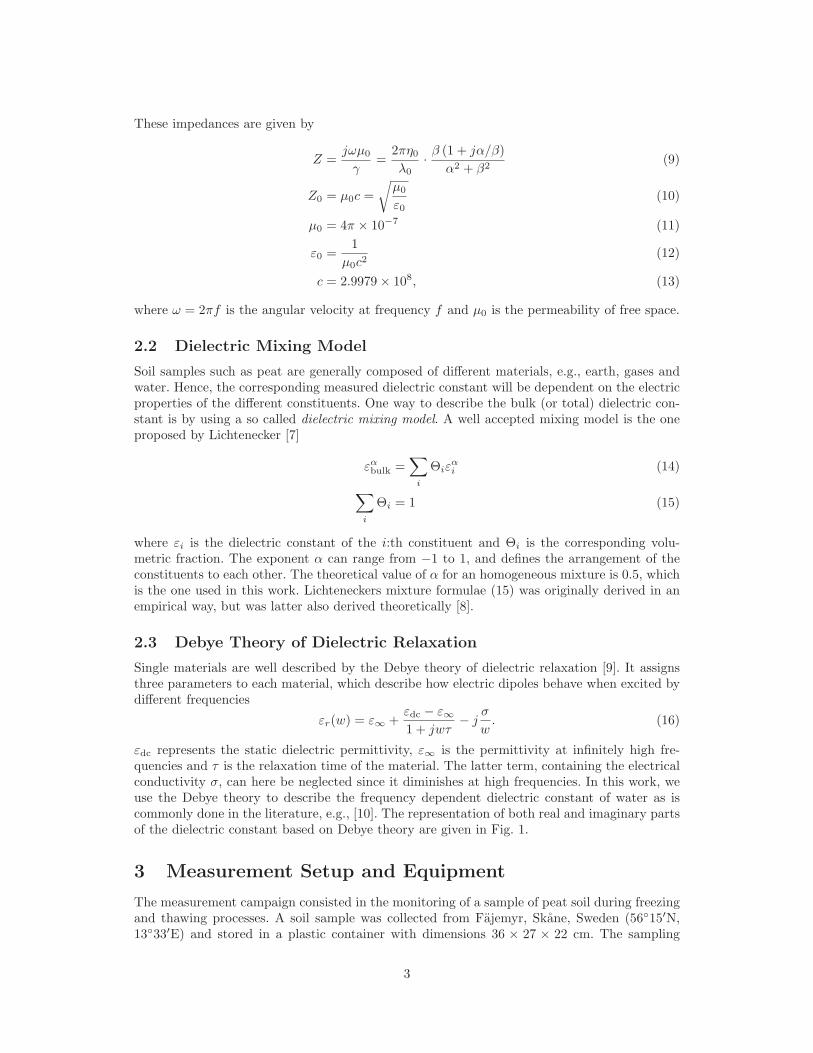
εdc represents the static dielectric permittivity, ε∞ is the permittivity at infinitely high fre-quencies and τ is the relaxation time of the material. The latter term, containing the electricalconductivity σ, can here be neglected since it diminishes at high frequencies. In this work, weuse the Debye theory to describe the frequency dependent dielectric constant of water as iscommonly done in the literature, e.g., [10]. The representation of both real and imaginary partsof the dielectric constant based on Debye theory are given in Fig. 1.

3 Measurement Setup and Equipment

The measurement campaign consisted in the monitoring of a sample of peat soil during freezingand thawing processes. A soil sample was collected from Fajemyr, Skane, Sweden (56◦15′N,13◦33′E) and stored in a plastic container with dimensions 36 × 27 × 22 cm. The sampling

3

Frequency [GHz]

Die

lect

ric

Con

stan

t

fmin

0.8 GHzfmax

3.3 GHz

ε′′(f)

ε′(f)

Debye theory

Measured

1 100

10

20

30

40

50

60

70

80

90

Figure 1: Theoretical and measured dielectric constant of water at 20◦ C.

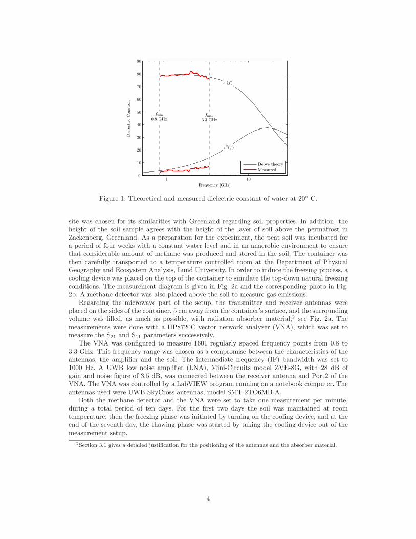
site was chosen for its similarities with Greenland regarding soil properties. In addition, theheight of the soil sample agrees with the height of the layer of soil above the permafrost inZackenberg, Greenland. As a preparation for the experiment, the peat soil was incubated fora period of four weeks with a constant water level and in an anaerobic environment to ensurethat considerable amount of methane was produced and stored in the soil. The container wasthen carefully transported to a temperature controlled room at the Department of PhysicalGeography and Ecosystem Analysis, Lund University. In order to induce the freezing process, acooling device was placed on the top of the container to simulate the top-down natural freezingconditions. The measurement diagram is given in Fig. 2a and the corresponding photo in Fig.2b. A methane detector was also placed above the soil to measure gas emissions.

Regarding the microwave part of the setup, the transmitter and receiver antennas wereplaced on the sides of the container, 5 cm away from the container’s surface, and the surroundingvolume was filled, as much as possible, with radiation absorber material,2 see Fig. 2a. Themeasurements were done with a HP8720C vector network analyzer (VNA), which was set tomeasure the S21 and S11 parameters successively.

The VNA was configured to measure 1601 regularly spaced frequency points from 0.8 to3.3 GHz. This frequency range was chosen as a compromise between the characteristics of theantennas, the amplifier and the soil. The intermediate frequency (IF) bandwidth was set to1000 Hz. A UWB low noise amplifier (LNA), Mini-Circuits model ZVE-8G, with 28 dB ofgain and noise figure of 3.5 dB, was connected between the receiver antenna and Port2 of theVNA. The VNA was controlled by a LabVIEW program running on a notebook computer. Theantennas used were UWB SkyCross antennas, model SMT-2TO6MB-A.

Both the methane detector and the VNA were set to take one measurement per minute,during a total period of ten days. For the first two days the soil was maintained at roomtemperature, then the freezing phase was initiated by turning on the cooling device, and at theend of the seventh day, the thawing phase was started by taking the cooling device out of themeasurement setup.

2Section 3.1 gives a detailed justification for the positioning of the antennas and the absorber material.

4

Cooling device

Soil sample

Notebook

GPIB

RF cable Port1 Port2

VectorNetworkAnalyzerHP8720C

Low NoiseAmplifier

LabVIEW

Radiationabsorbingmaterial

Methanedetector

(a) Measurement diagram.

antenna

soilVNA

LNARF cable

notebook

(b) Photo of the measurement setup.

Figure 2: Measurement diagram and corresponding photo at the temperature controlled room,Department of Physical Geography and Ecosystem Analysis, Lund University. Photo takenduring the preparation for the measurements.

5

Am

plitu

de

[dB

]

Standard setup

Frequency [GHz]

Am

plitu

de

[dB

]

air-filled box

water-filled box

Improved setup

1 1.5 2 2.5 3

1 1.5 2 2.5 3

-100

-80

-60

-40

-20

0

-100

-80

-60

-40

-20

0

Figure 3: Uncalibrated S21 parameter values for standard (upper plot) and improved (lowerplot) measurement setup .

3.1 Reducing Undesired Diffraction and Reflection Effects

In order to find the dielectric constant of the material, we assume that the measured S21

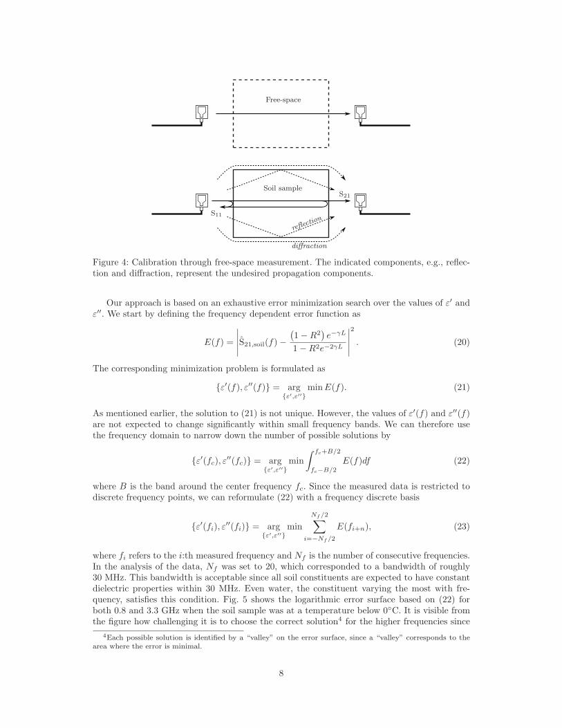
parameters are well modeled by the transmission equation (1). However, considering the sizeof our sample, this approximation is only true if the microwave signals arriving at the receiverantenna are only propagating in a straight line from the transmitter antenna, i.e., no additionalcomponents exist. In practice, this is impossible to achieve as diffraction components around thesample and reflection components from within the sample will always exist, these are illustratedin Fig. 4. In an effort to minimize these undesired effects we used the following measurementsetup:

• Radiation absorbing material was placed on the sides of the plastic box to minimize thediffracted fields.

• The antennas were placed 5 cm away from the box, such that the waves propagatingthrough the sample are more flat, i.e., less spherical, which reduces the strength of thereflection components on the sides of the container. In addition, the antenna mismatchwas also reduced since the used antennas are designed for transmission in air.

A representation of the position of the absorbers and the antennas is given in Fig. 2a. In orderto quantify the improvements, test measurements were performed considering an empty boxand water-filled box, see Fig. 3. From the upper plot, it is visible how strong the diffractioncomponents are. For the lower frequencies, the transmission through water is larger than thetransmission in free-space, which is physically impossible if not considering diffraction aroundthe box. By applying the above referred modifications to the measurement setup, the diffractedand reflected fields were generally reduced. This reduction was more significant at the lowerfrequencies, e.g., at 1 GHz the power was reduced by 40 dB. The results shown in the lower plotof Fig. 3 are more acceptable: the transmission through water is always below transmission infree-space and the difference between the two lines increases with frequency, which agrees withthe water property of increasing loss with increasing frequency.

6

4 Data Analysis and Post-Processing

4.1 Calibration

When transmission measurements are done through a sample, the recorded S21 parameterincludes not only the influence of the sample under test but also the antenna distortions. Tocorrect for this, the measured S21 must be calibrated.3 A simple way to perform this calibrationis to do it directly in the frequency domain by a division, as is done by [11],

S21,soil(f) =S21,mea.(f)

S21,cal.(f). (17)

It is important to note that calibrations performed directly by a division, are only valid undercertain conditions. One condition is that the system must be linear and that the introductionof a certain material in the box must not generate additional propagation components, e.g.,diffraction and reflection components, as represented in Fig. 4. This in often not the case asmaterials with ε′ > 1 generate diffraction fields around the sample and create new reflectedcomponents from within the sample. To find the correction coefficients, S21,cal.(f), we startedby measuring the transmission through an empty box, which contained all the referred non-linearities, S21,free-space(f). Ideally, S21,cal.(f) should be the transmission coefficient for whenthere is no sample at all, such that the antennas would have to be almost touching each other.This is not possible since the two antennas would stop behaving has good radiators due tothe coupling between each other. So, our approach is to first measure the empty box (freespace), and then “back-rotate” the phase of each one of the frequency points by an amountcorresponding to the length of the box L, assuming propagation at the speed of light. In thisway, we eliminate the influence of the unwanted free space within the box

S21,cal.(f) = S21,free-space(f) · ej2πLf/c (18)

= S21,free-space(f) · ejwτ0 . (19)

where τ0 is the propagation delay corresponding to a wave traveling at the speed of light througha length of L. This approach also solves an additional problem. The assumption in equation(1) is that the wave impinging on the slab is plane, or lossless, which is not our case since thewaves radiated by the antennas are spherical, and therefore lossy. However, the same sphericalloss is also measured in S21,free-space(f), and will therefore be compensated in (17).

It is important to refer that the above described calibration does not replace the internalcalibration of the VNA, which corrects for the equipment’s internal errors and non-linearities[12]. However, the internal calibration of the VNA is not sufficient since it is not able to correctfor the antenna distortions.

4.2 Calculation of the Dielectric Parts ε′ and ε

′′

The calculation of the dielectric constant is not trivial because there is no direct relation betweenε′ or ε′′, and the measured S21 parameter. One approach is to use numerical methods. Severaliterative numerical methods have been proposed in the literature, in [5] an iterative algorithmbased on (6) and (7) is proposed. The drawback of such algorithms is generally the uncertaintyoff the convergence to the correct solution, which is usually dependent on the initial values.The non-unique solution, i.e., the fact that several values of ε′ and ε′′ verify (1) and (2), stemsfrom the repetitive nature of a sinusoidal wave.

3Calibration is also referred to as “correction.”

7

Free-space

Soil sample

reflecti

on

diffraction

S11

S21

Figure 4: Calibration through free-space measurement. The indicated components, e.g., reflec-tion and diffraction, represent the undesired propagation components.

Our approach is based on an exhaustive error minimization search over the values of ε′ andε′′. We start by defining the frequency dependent error function as

E(f) =

∣

∣

∣

∣

∣

S21,soil(f) −(

1 − R2)

e−γL

1 − R2e−2γL

∣

∣

∣

∣

∣

2

. (20)

The corresponding minimization problem is formulated as

{ε′(f), ε′′(f)} = arg{ε′,ε′′}

min E(f). (21)

As mentioned earlier, the solution to (21) is not unique. However, the values of ε′(f) and ε′′(f)are not expected to change significantly within small frequency bands. We can therefore usethe frequency domain to narrow down the number of possible solutions by

{ε′(fc), ε′′(fc)} = arg

{ε′,ε′′}

min

∫ fc+B/2

fc−B/2

E(f)df (22)

where B is the band around the center frequency fc. Since the measured data is restricted todiscrete frequency points, we can reformulate (22) with a frequency discrete basis

{ε′(fi), ε′′(fi)} = arg

{ε′,ε′′}

min

Nf /2∑

i=−Nf /2

E(fi+n), (23)

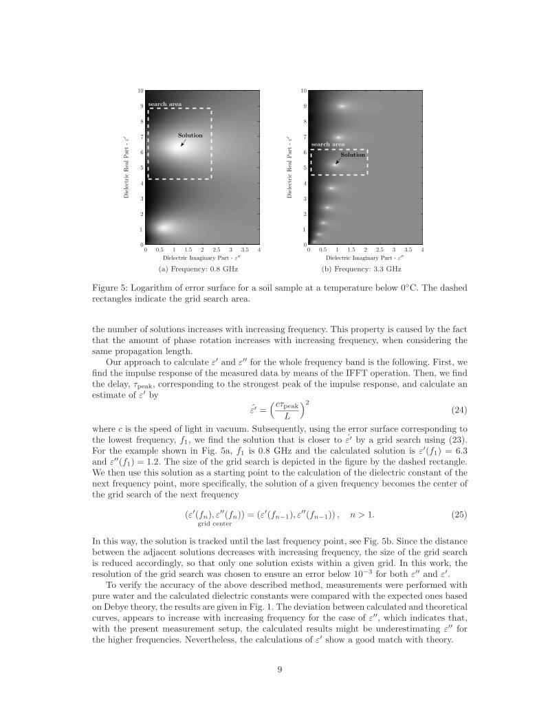
where fi refers to the i:th measured frequency and Nf is the number of consecutive frequencies.In the analysis of the data, Nf was set to 20, which corresponded to a bandwidth of roughly30 MHz. This bandwidth is acceptable since all soil constituents are expected to have constantdielectric properties within 30 MHz. Even water, the constituent varying the most with fre-quency, satisfies this condition. Fig. 5 shows the logarithmic error surface based on (22) forboth 0.8 and 3.3 GHz when the soil sample was at a temperature below 0◦C. It is visible fromthe figure how challenging it is to choose the correct solution4 for the higher frequencies since

4Each possible solution is identified by a “valley” on the error surface, since a “valley” corresponds to thearea where the error is minimal.

8

Dielectric Imaginary Part - ε′′

Die

lect

ric

Rea

lPar

t-

ε′

Solution

search area

0 0.5 1 1.5 2 2.5 3 3.5 4

10

9

8

7

6

5

4

3

2

1

0

(a) Frequency: 0.8 GHz

Dielectric Imaginary Part - ε′′

Die

lect

ric

Rea

lPar

t-

ε′

search area

Solution

0 0.5 1 1.5 2 2.5 3 3.5 4

10

9

8

7

6

5

4

3

2

1

0

(b) Frequency: 3.3 GHz

Figure 5: Logarithm of error surface for a soil sample at a temperature below 0◦C. The dashedrectangles indicate the grid search area.

the number of solutions increases with increasing frequency. This property is caused by the factthat the amount of phase rotation increases with increasing frequency, when considering thesame propagation length.

Our approach to calculate ε′ and ε′′ for the whole frequency band is the following. First, wefind the impulse response of the measured data by means of the IFFT operation. Then, we findthe delay, τpeak, corresponding to the strongest peak of the impulse response, and calculate anestimate of ε′ by

ε′ =(cτpeak

L

)2

(24)

where c is the speed of light in vacuum. Subsequently, using the error surface corresponding tothe lowest frequency, f1, we find the solution that is closer to ε′ by a grid search using (23).For the example shown in Fig. 5a, f1 is 0.8 GHz and the calculated solution is ε′(f1) = 6.3and ε′′(f1) = 1.2. The size of the grid search is depicted in the figure by the dashed rectangle.We then use this solution as a starting point to the calculation of the dielectric constant of thenext frequency point, more specifically, the solution of a given frequency becomes the center ofthe grid search of the next frequency

(ε′(fn), ε′′(fn))grid center

= (ε′(fn−1), ε′′(fn−1)) , n > 1. (25)

In this way, the solution is tracked until the last frequency point, see Fig. 5b. Since the distancebetween the adjacent solutions decreases with increasing frequency, the size of the grid searchis reduced accordingly, so that only one solution exists within a given grid. In this work, theresolution of the grid search was chosen to ensure an error below 10−3 for both ε′′ and ε′.

To verify the accuracy of the above described method, measurements were performed withpure water and the calculated dielectric constants were compared with the expected ones basedon Debye theory, the results are given in Fig. 1. The deviation between calculated and theoreticalcurves, appears to increase with increasing frequency for the case of ε′′, which indicates that,with the present measurement setup, the calculated results might be underestimating ε′′ forthe higher frequencies. Nevertheless, the calculations of ε′ show a good match with theory.

9

Table 1: Considered dielectric permittivities of the three soil constituents.

ε1 gas ε2 water ε3 solid

ε′ 1 Debye (16) 3.150ε′′ 0 Debye (16) 0.005

4.3 Dielectric Properties of the Constituent Materials

For the considerations regarding the dielectric properties of the constituent materials, we followthe reasoning presented in [13]. In brief, we model the soil samples by three constituents: gas,water and solid, such that the corresponding volumetric fractions verify

Θ1gas

+ Θ2water

+ Θ3solid

= 1, Θ1,Θ2,Θ3 ≥ 0. (26)

4.4 Calculation of the Volumetric Fractions

The aim of this work is ultimately to find the value of these three parameters for every timeinstant.5 In order to find the three volumetric fractions, we make use of the calculated dielectricconstants together with the mixing model described in section 2.2, such that

√εcalc. = Θ1

√ε1 + Θ2

√ε2 + Θ3

√ε3 (27)

where εcalc. = ε′ − jε′′ denotes the dielectric constant calculated from the method described inSection 4.2. The values chosen for ε1, ε2 and ε3 are given in Table 1, and the correspondingjustification is provided in [13]. Considering Eq. (26), together with the fact that Eq. (27) iscomplex and therefore needs to be valid independently for the real and imaginary parts, wearrive at a system of three equations

Re {√εcalc.} = Re {Θ1

√ε1 + Θ2

√ε2 + Θ3

√ε3} (28)

Im {√εcalc.} = Im {Θ1

√ε1 + Θ2

√ε2 + Θ3

√ε3} (29)

1 = Θ1 + Θ2 + Θ3 (30)

from which the three unknowns Θ1, Θ2 and Θ3 can be calculated.However, the calculation of the volumetric fractions is not straightforward since the above

system of equations is non-linear. Following the same approach used for the calculation of ε′

and ε′′ in Section 4.2, we avoid iterative methods and estimate the three unknowns by meansof a fine grid search. By replacing (30) on (28) and (29), the problem can be simplified to atwo-dimensional grid search.

5 Results

5.1 Frequency and Time Domain Profiles

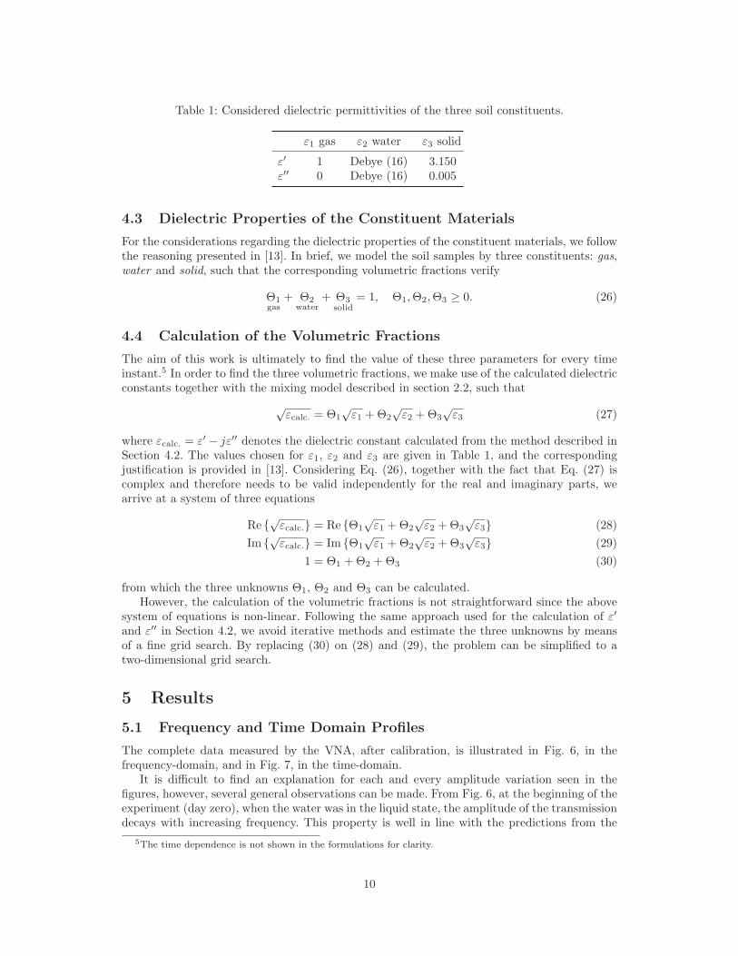
The complete data measured by the VNA, after calibration, is illustrated in Fig. 6, in thefrequency-domain, and in Fig. 7, in the time-domain.

It is difficult to find an explanation for each and every amplitude variation seen in thefigures, however, several general observations can be made. From Fig. 6, at the beginning of theexperiment (day zero), when the water was in the liquid state, the amplitude of the transmissiondecays with increasing frequency. This property is well in line with the predictions from the

5The time dependence is not shown in the formulations for clarity.

10

Time [days]

Fre

quen

cy[G

Hz]

Am

plitu

de

[dB

]

Freezing ThawingStatic

0 2 4 6 8-70

-60

-50

-40

-30

-20

-10

0

3

2.5

2

1.5

1

Figure 6: Measured S21 parameter after calibration, for the full ten days of measurements.

Debye model for water. Then, during the freezing phase, while the liquid water was progressivelybeing transformed into solid ice, the higher frequencies progressively became less attenuated(at 3.3 GHz, from day two to day eight, there is an increase in received power of 40 dB). On theother hand, the attenuation of the lower frequencies (e.g., 0.8 GHz) barely changes during thesix days of freezing, which also agrees with the Debye model. On the onset of the thawing phase,there is an increase in the volumetric content of liquid water, and the transmission coefficientnaturally decreases.

The data presented in Fig. 7, results from applying the IFFT operation to the calibrated S21

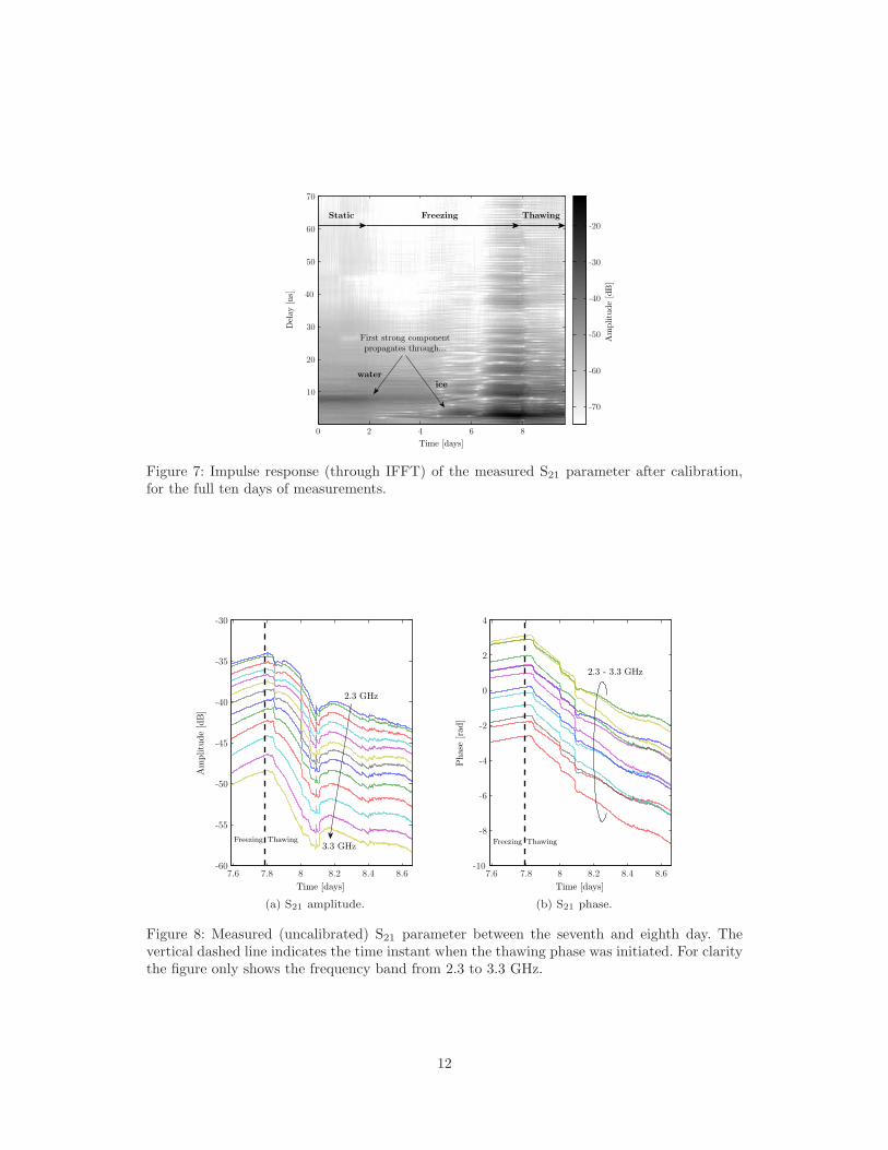
parameter, and in the figure, there are two aspects worth mentioning: 1) As indicated by thetwo arrows, the first strong component of the impulse response appears at 8 ns before freezingand at 2 ns after freezing. This indicates that at the start of the measurements, the transmittedpulse6 propagates mainly through liquid water, and that at day eight the propagation is mademainly through ice. It is also notable that around day four, there are two arriving componentswith comparable amplitude at delays 3 ns and 8 ns, which point to the fact that, at this instant,there were two separable layers in the soil: a top-frozen layer and a bottom-unfrozen one. 2)Between day six and day eight, a train of amplitude decreasing pulses is visible along the delaydomain. This supports the idea that the received power is not only due to one componentthat propagates through the soil once, but also due to later propagation components which arereflected multiple times from within the soil. This is a characteristic of dielectric slabs with lowε′′, as is the case of ice.

5.2 Amplitude and Phase Variations versus Methane Emissions

Regarding methane emissions, these were only detected during the thawing phase, and thereforewe now focus our attention to the results from day 7.6 to day 8.6. From Figs. 6 and 7, the am-plitude variations in this period appear very smooth. However, when looking with more detail,several sharp small-scale variations (< 1 dB) are visible, see Fig. 8a. These sharp variations areboth positive, i.e., increase of amplitude, and negative, i.e., decrease of amplitude. The phaseof S21 shows similar variations as shown in Fig. 8b.

To better understand the relation between the variations of both the amplitude and phasewith the emissions of methane, we plot their time derivatives together for comparison, see Fig. 9.A peak in the derivative of the methane flux, corresponds to a burst emission of methane from

6By “pulse,” we refer to the virtual time-domain “sinc” pulse composed of all the transmitted frequencies.

11

Time [days]

Del

ay[n

s]

Am

plitu

de

[dB

]

Static Freezing Thawing

water

ice

First strong componentpropagates through...

0 2 4 6 8

-70

-60

-50

-40

-30

-20

70

60

50

40

30

20

10

Figure 7: Impulse response (through IFFT) of the measured S21 parameter after calibration,for the full ten days of measurements.

Time [days]

Am

plitu

de

[dB

]

Freezing Thawing

2.3 GHz

3.3 GHz

7.6 7.8 8 8.2 8.4 8.6-60

-55

-50

-45

-40

-35

-30

(a) S21 amplitude.

Time [days]

Phas

e[r

ad]

Freezing Thawing

2.3 - 3.3 GHz

7.6 7.8 8 8.2 8.4 8.6-10

-8

-6

-4

-2

0

2

4

(b) S21 phase.

Figure 8: Measured (uncalibrated) S21 parameter between the seventh and eighth day. Thevertical dashed line indicates the time instant when the thawing phase was initiated. For claritythe figure only shows the frequency band from 2.3 to 3.3 GHz.

12

Nor

m.der

ivat

ives

[?/m

in]

Methane fluxS21 amplitude

Time [days]

Nor

m.der

ivat

ives

[?/m

in]

Methane fluxS21 phase

7.8 7.9 8 8.1 8.2 8.3 8.4 8.5 8.6-4

-2

0

2

4-4

-2

0

2

4

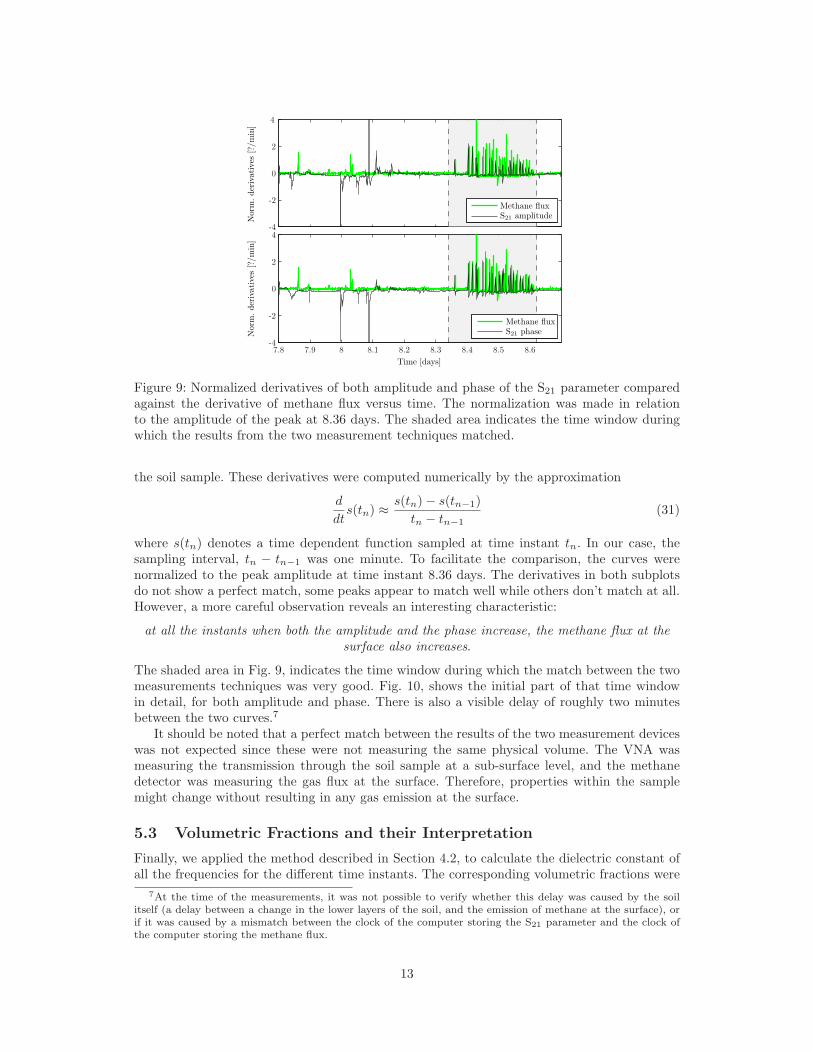
Figure 9: Normalized derivatives of both amplitude and phase of the S21 parameter comparedagainst the derivative of methane flux versus time. The normalization was made in relationto the amplitude of the peak at 8.36 days. The shaded area indicates the time window duringwhich the results from the two measurement techniques matched.

the soil sample. These derivatives were computed numerically by the approximation

d

dts(tn) ≈ s(tn) − s(tn−1)

tn − tn−1

(31)

where s(tn) denotes a time dependent function sampled at time instant tn. In our case, thesampling interval, tn − tn−1 was one minute. To facilitate the comparison, the curves werenormalized to the peak amplitude at time instant 8.36 days. The derivatives in both subplotsdo not show a perfect match, some peaks appear to match well while others don’t match at all.However, a more careful observation reveals an interesting characteristic:

at all the instants when both the amplitude and the phase increase, the methane flux at the

surface also increases.

The shaded area in Fig. 9, indicates the time window during which the match between the twomeasurements techniques was very good. Fig. 10, shows the initial part of that time windowin detail, for both amplitude and phase. There is also a visible delay of roughly two minutesbetween the two curves.7

It should be noted that a perfect match between the results of the two measurement deviceswas not expected since these were not measuring the same physical volume. The VNA wasmeasuring the transmission through the soil sample at a sub-surface level, and the methanedetector was measuring the gas flux at the surface. Therefore, properties within the samplemight change without resulting in any gas emission at the surface.

5.3 Volumetric Fractions and their Interpretation

Finally, we applied the method described in Section 4.2, to calculate the dielectric constant ofall the frequencies for the different time instants. The corresponding volumetric fractions were

7At the time of the measurements, it was not possible to verify whether this delay was caused by the soilitself (a delay between a change in the lower layers of the soil, and the emission of methane at the surface), orif it was caused by a mismatch between the clock of the computer storing the S21 parameter and the clock ofthe computer storing the methane flux.

13

Nor

m.der

ivat

ives

[?/m

in]

Methane fluxS21 amplitude

Time [days]

Nor

m.der

ivat

ives

[?/m

in]

Methane fluxS21 phase

8.34 8.36 8.38 8.4 8.42 8.44 8.46 8.48-1

0

1

2

3

4-1

0

1

2

3

4

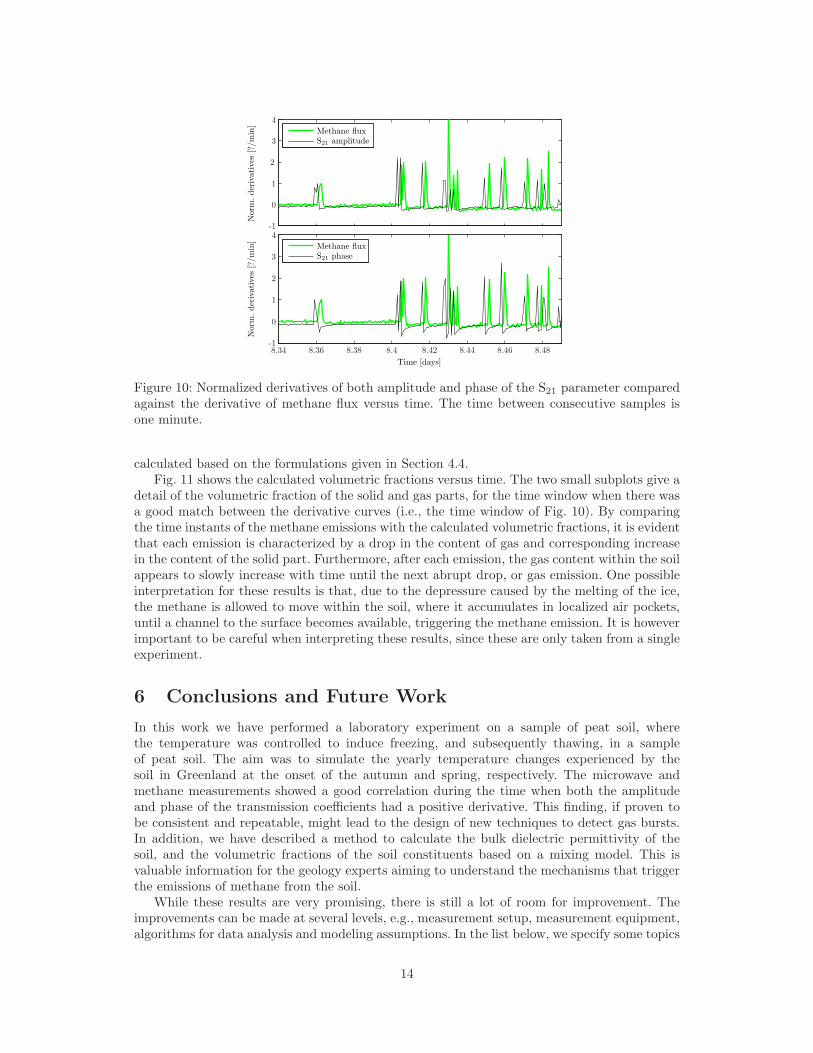
Figure 10: Normalized derivatives of both amplitude and phase of the S21 parameter comparedagainst the derivative of methane flux versus time. The time between consecutive samples isone minute.

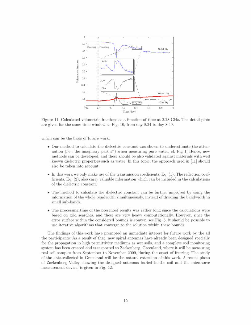
calculated based on the formulations given in Section 4.4.Fig. 11 shows the calculated volumetric fractions versus time. The two small subplots give a

detail of the volumetric fraction of the solid and gas parts, for the time window when there wasa good match between the derivative curves (i.e., the time window of Fig. 10). By comparingthe time instants of the methane emissions with the calculated volumetric fractions, it is evidentthat each emission is characterized by a drop in the content of gas and corresponding increasein the content of the solid part. Furthermore, after each emission, the gas content within the soilappears to slowly increase with time until the next abrupt drop, or gas emission. One possibleinterpretation for these results is that, due to the depressure caused by the melting of the ice,the methane is allowed to move within the soil, where it accumulates in localized air pockets,until a channel to the surface becomes available, triggering the methane emission. It is howeverimportant to be careful when interpreting these results, since these are only taken from a singleexperiment.

6 Conclusions and Future Work

In this work we have performed a laboratory experiment on a sample of peat soil, wherethe temperature was controlled to induce freezing, and subsequently thawing, in a sampleof peat soil. The aim was to simulate the yearly temperature changes experienced by thesoil in Greenland at the onset of the autumn and spring, respectively. The microwave andmethane measurements showed a good correlation during the time when both the amplitudeand phase of the transmission coefficients had a positive derivative. This finding, if proven tobe consistent and repeatable, might lead to the design of new techniques to detect gas bursts.In addition, we have described a method to calculate the bulk dielectric permittivity of thesoil, and the volumetric fractions of the soil constituents based on a mixing model. This isvaluable information for the geology experts aiming to understand the mechanisms that triggerthe emissions of methane from the soil.

While these results are very promising, there is still a lot of room for improvement. Theimprovements can be made at several levels, e.g., measurement setup, measurement equipment,algorithms for data analysis and modeling assumptions. In the list below, we specify some topics

14

Freezing Thawing

Time [days]

Vol

um

etri

cFra

ctio

n

Solid Θ3

Water Θ2

Gas Θ1

Solid

Gas

7.6 7.8 8 8.2 8.4 8.6 8.8 90

0.1

0.2

0.3

0.4

0.5

0.6

0.7

0.8

0.9

1

Figure 11: Calculated volumetric fractions as a function of time at 2.28 GHz. The detail plotsare given for the same time window as Fig. 10, from day 8.34 to day 8.49.

which can be the basis of future work:

• Our method to calculate the dielectric constant was shown to underestimate the atten-uation (i.e., the imaginary part ε′′) when measuring pure water, cf. Fig 1. Hence, newmethods can be developed, and these should be also validated against materials with wellknown dielectric properties such as water. In this topic, the approach used in [11] shouldalso be taken into account.

• In this work we only make use of the transmission coefficients, Eq. (1). The reflection coef-ficients, Eq. (2), also carry valuable information which can be included in the calculationsof the dielectric constant.

• The method to calculate the dielectric constant can be further improved by using theinformation of the whole bandwidth simultaneously, instead of dividing the bandwidth insmall sub-bands.

• The processing time of the presented results was rather long since the calculations werebased on grid searches, and these are very heavy computationally. However, since theerror surface within the considered bounds is convex, see Fig. 5, it should be possible touse iterative algorithms that converge to the solution within these bounds.

The findings of this work have prompted an immediate interest for future work by the allthe participants. As a result of that, new spiral antennas have already been designed speciallyfor the propagation in high permittivity mediums as wet soils, and a complete soil monitoringsystem has been created and transported to Zackenberg, Greenland, where it will be measuringreal soil samples from September to November 2009, during the onset of freezing. The studyof the data collected in Greenland will be the natural extension of this work. A recent photoof Zackenberg Valley showing the designed antennas buried in the soil and the microwavemeasurement device, is given in Fig. 12.

15

Figure 12: Photo of Zackenberg Valley in Greenland, taken on August 25th, 2009. The mi-crowave measurement device is a Rohde&Schwarz FSH4 Handheld Network Analyzer.

7 Acknowledgements

The help of Norbert Pirk, Mikhail Mastepanov and Torben R. Christensen from the Departmentof Physical Geography and Ecosystem Analysis, Lund University, is greatly appreciated, bothduring the measurements and during the analysis of the data. The initial idea to use microwavemeasurements was Norbert’s. We also thank LUNARC, the center for scientific and technicalcomputing for research at Lund University, for providing the vital access to their cluster ofcomputers. This work was financially supported, in part, by the Swedish Strategic ResearchFoundation (SSF) Center of High Speed Wireless Communications (HSWC) at Lund Universityand by the Swedish Vetenskapsradet.

References

[1] O. A. Anisimov, “Potential feedback of thawing permafrost to the global climate systemthrough methane emission,” Environmental Research Letters, vol. 2, no. 4, Nov. 2007.

[2] D. J. Wuebbles and K. Hayhoe, “Atmospheric methane and global change,” Earth-Science

Reviews, vol. 57, no. 3-4, pp. 177 – 210, May 2002.

[3] M. Mastepanov, C. Sigsgaard, E. J. Dlugokencky, S. Houweling, L. Strom, M. P. Tamstorf,and T. R. Christensen, “Large tundra methane burst during onset of freezing,” Nature,vol. 456, no. 7222, pp. 628–630, Dec. 2008.

[4] A. M. Nicolson and G. F. Ross, “Measurement of the intrinsic properties of materials bytime-domain techniques,” IEEE Trans. Instrum. Meas., vol. 19, no. 4, pp. 377–382, Nov.1970.

[5] M. T. Hallikainen, F. T. Ulaby, M. C. Dobson, M. A. El-Rayes, and L.-K. Wu, “Microwavedielectric behavior of wet soil – part I: Empirical models and experimental observations,”IEEE Transactions on Geoscience and Remote Sensing, vol. GE-23, pp. 25–34, Jan. 1985.

[6] E. H. Kansson, A. Amiet, and A. Kaynak, “Dielectric characterization of conducting tex-tiles using free space transmission measurements: Accuracy and methods for improvement,”Synthetic Metals, vol. 157, no. 24, pp. 1054 – 1063, Dec. 2007.

16

[7] K. Lichtenecker, “Dielectric constant of natural and synthetic mixtures,” Phys. Z, 1926.

[8] Z. Tarik, L. Jean-Paul, and V. Michel, “Theoretical evidence for ‘Lichtenecker’s mixtureformulae’ based on the effective medium theory,” Journal of Physics D: Applied Physics,vol. 31, no. 13, pp. 1589–1594, 1998.

[9] P. Debye, Polar Molecules. Chemical Catalog Co. New York (reprinted by Dover, NewYork, 1954), 1929.

[10] J. O. Curtis, “A durable laboratory apparatus for the measurement of soil dielectric prop-erties,” IEEE Transactions on Instrumentation and Measurement, vol. 50, no. 5, pp. 1364–1369, Oct. 2001.

[11] A. Muqaibel, “Characterization of ultra wideband communication channels,” Ph.D. dis-sertation, Virginia Polytechnic Institute and State University, 2003.

[12] D. Ballo, “Network analyzer basics – Back to basics seminar,” Hewlett-Packard, 1998.

[13] N. Pirk, “Methane emission peaks from permafrost environments: Using ultra-widebandspectroscopy, sub-surface pressure sensing and finite element solving as means of theirexploration,” Master’s thesis, Department of Physical Geography and Ecosystems Analysis,Lund University, June 2009.

17