38
Di/erentiated Products Demand Systems (B) Jonathan Levin Economics 257 Stanford University Fall 2009 Jonathan Levin Demand Estimation Fall 2009 1 / 38

Di¤erentiated Products Demand Systems (B)
Jonathan Levin
Economics 257Stanford University
Fall 2009
Jonathan Levin (Economics 257 Stanford University)Demand Estimation Fall 2009 1 / 38

Demand in characteristic space: introduction
Theory can be divided to two:
Price competition, taking products as given (see Caplin and Nalebu¤,1991, who provide conditions for existence for a wide set of models)Competition in product space with or without subsequent pricecompetition (e.g. Hotelling on a line, Salop on a circle, etc.).
The empirical literature is almost entirely focused on the former, andthere is much room for empirical analysis of the latter.
Moreover, much of the demand literature uses the characteristics asinstruments. This is both ine¢ cient (why?) and probably inconsistent(why?); we all recognize it, but keep doing it without goodalternatives (we will come back to it later).
Jonathan Levin (Economics 257 Stanford University)Demand Estimation Fall 2009 2 / 38

Characteristic space: overview
Products are bundles of characteristics, and consumers havepreferences over these characteristics.
Typically, we use a discrete choice approach: consumers choose oneproduct only. Di¤erent consumers have di¤erent characteristics, so inthe aggregate all products are chosen.
Aggregate demand depends on the entire distribution of consumers.
Jonathan Levin (Economics 257 Stanford University)Demand Estimation Fall 2009 3 / 38

Characteristic space: overview
Formally, consumer i has the following utility from product j :
Uij = U(Xj , pj , νi ; θ)
We typically think of j = 0, 1, 2, ..., J, where product 0 is the outsidegood (why do we need it?).
Consumer i�s choice is the product which maximizes her utility, i.e.she chooses product j i¤ Uij � Uik for all k. She chooses only oneunit of one product, by assumption (how bad is this assumption?).
Predicted market share for product j is therefore
sj (θ) =ZI (νi 2 fνjU(Xj , pj , ν; θ) � U(Xk , pk , ν; θ)8kg) dF (νi )
Note: utility is invariant to monotone transformations, so we need tonormalize. Typically: set Ui0 = 0 and �x one of the parameters or thevariance of the error.
Jonathan Levin (Economics 257 Stanford University)Demand Estimation Fall 2009 4 / 38

Characteristic choice: examples
Two goods: j = 0, 1, 2. Uij = δj + εij (and Ui0 = 0).
Hotelling with quadratic transportation costs:
Uij = u + (yi � pj ) + θd2(xj , νi )
Vertical model: Uij = δj � υipj (υi > 0). What makes it vertical?example: �rst class, business, economy.
Logit:Uij = u + (yi � pj ) + δj + εij
where the ε�s are distributed extreme value i.i.d across i and j(F (x) = e�e
�x). It looks like normal, but with fatter tails.
A key feature of this distributional assumption is that it gives us aclosed-form solution for the integral over the max.
Jonathan Levin (Economics 257 Stanford University)Demand Estimation Fall 2009 5 / 38

Characteristic choice (cont.)
In general, we can classify the models into two main classes:1 Uij = f (yi , pj ) + δj +∑k βk xjk νik (Berry and Pakes, 2002, �PureHedonic�) orUij = f (yi , pj ) + δj +∑k αk (xjk � νik )
2 (Anderson, de Palma, andThisse, 1992: �Ideal Type�), with fy > 0, fp < 0, fpy � 0.
2 Uij = f (yi , pj ) + δj +∑k βk xjk νik + εij (Berry, Levinsohn, and Pakes,1995)
The key di¤erence is the εij . With the εij the product space can neverbe exhausted: each new product comes with a whole new set of εij�s,guaranteeing itself a positive market share and some market power.This may lead to problematic results in certain contexts, such as theanalysis of new goods.
Instruments: typically we assume X is exogenous, so we useinstruments that are either cost shifters or functions of X which arelikely to be correlated with markups.
Jonathan Levin (Economics 257 Stanford University)Demand Estimation Fall 2009 6 / 38

The vertical model
Utility is given byUij = δj � υipj (υi > 0)
So if pj > pk and qj > 0, we must have δj > δk .Therefore, we order the products according to their price (andquality), say in an increasing order.Consumer i prefers product j over j + 1 i¤ δj � υipj > δj+1 � υipj+1and over j � 1 i¤ δj � υipj > δj�1 � υipj�1. Due to single-crossingproperty, these two are su¢ cient to make sure that consumer ichooses j (verify as an exercise).Therefore, consumer i chooses product j i¤:
δj+1 � δjpj+1 � pj
< νi <δj � δj�1pj � pj�1
which implies a set of n cuto¤ points (see �gure).Note that, as usual, we normalize the utility from the outside good tobe zero for all consumers.
Jonathan Levin (Economics 257 Stanford University)Demand Estimation Fall 2009 7 / 38

The vertical model (cont.)
Given a distribution for ν we now have the market share for product jpredicted by
F�
δj � δj�1pj � pj�1
�� F
�δj+1 � δjpj+1 � pj
�Given the distribution and an assumption about the size of the overallmarket we obtain a one-to-one mapping from the market shares tothe δ�s, so we can estimate by imposing structures on the δ�s and thedistribution.
Note that the vertical model has the property that only prices ofadjacent (in terms of prices) products a¤ect the market share, soprice elasticity with respect to all other products is zero.
Is this reasonable? This is a major restriction on the data, anddepending on the context you want to think carefully if this is anassumption you want to impose, or that it is too restrictive.
Jonathan Levin (Economics 257 Stanford University)Demand Estimation Fall 2009 8 / 38

Econometric digression
So far we assumed that we observe market shares precisely, i.e. thatmarket share data is based on the choice of �in�nitely�manyconsumers.
This is not always the case (e.g. Berry, Carnall, and Spiller, 1997). Insuch cases we can get the likelihood of the data to be given by amultinomial distribution of outcomes.
This gives usL _ ∏
jsj (θ)nj
so that
θ = argmax [ln L] = argmax
"∑jsoj ln sj (θ)
#
Jonathan Levin (Economics 257 Stanford University)Demand Estimation Fall 2009 9 / 38

Econometric digression
Asymptotically (when soj = sj (θ)) this is equivalent to
argmin
264∑j
�soj � sj (θ)
�2sj (θ)2
375which is called a minimum χ2 (or a modi�ed minimum χ2 when sj (θ)is replaced by soj in the denominator).
This just shows that we should get a better �t on products withsmaller market shares. It also shows why we may face more problemswhen we have tiny market shares.
Jonathan Levin (Economics 257 Stanford University)Demand Estimation Fall 2009 10 / 38
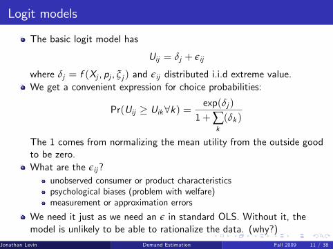
Logit models
The basic logit model has
Uij = δj + εij
where δj = f (Xj , pj , ξ j ) and εij distributed i.i.d extreme value.We get a convenient expression for choice probabilities:
Pr(Uij � Uik8k) =exp(δj )
1+∑k
(δk )
The 1 comes from normalizing the mean utility from the outside goodto be zero.What are the εij?
unobserved consumer or product characteristicspsychological biases (problem with welfare)measurement or approximation errors
We need it just as we need an ε in standard OLS. Without it, themodel is unlikely to be able to rationalize the data. (why?)
Jonathan Levin (Economics 257 Stanford University)Demand Estimation Fall 2009 11 / 38

Logit models (cont.)
Suppose further that
δj = Xjβ� αpj + ξ j
We can rearrange the market share equation to have δj = ln sj � ln s0,so we have a linear equation we can estimate:
ln sj � ln s0 = Xjβ� αpj + ξ j
The linear form is very useful. We can now instrument for prices usingstandard IV procedures. This is the main reason people use logit somuch: it�s �cheap� to do, so you might as well see what it gives you.
Jonathan Levin (Economics 257 Stanford University)Demand Estimation Fall 2009 12 / 38

Logit models: caveats
Basic logit model
ln sj � ln s0 = Xjβ� αpj + ξ j
Key drawback: problematic implications for own- andcross-elasticities. To see this, note (and verify at home) that∂sj∂pj= �αsj (1� sj ) and ∂sj
∂pk= αsj sk . So:
Own-elasticity - ηj =∂sj∂pj
pjsj= �αpj (1� sj ) - is increasing in price,
which is somewhat unrealistic (we would think people who buyexpensive products are less sensitive to price).
Cross-elasticity - ηjk =∂sj∂pk
pksj= αpk sk - depends only on market
shares and prices but not on similarities between goods (think ofexamples). This is typically called IIA property.
Jonathan Levin (Economics 257 Stanford University)Demand Estimation Fall 2009 13 / 38

Logit models (cont.)
Most of the extensions try to correct for the above. Mostly this is notjust an issue of the distributional assumption. (What would happenwith probit error term?)Note that if we just care about dsj/dxj and not the elasticity matrix,logit may be good enough. Always remember: whether it is good ornot cannot be determined in isolation; it depends on the way it isbeing used.Why do we need ξ j? this is the analog to the demand-and-supplymodel, and create the �exibility for us to �t the model. This alsoshows explicitly the endogeneity of prices, because they are likely todepend on ξ j and this is why we need to instrument for them(examples).Instruments are typically based on the mean independenceassumption, i.e. E (ξ j jX ) = 0. Does this make sense? What are theassumptions that need to be made to make this go through? Ispre-determination su¢ cient?
Jonathan Levin (Economics 257 Stanford University)Demand Estimation Fall 2009 14 / 38

Nested logit
The basic idea is to relax IIA by grouping the products (somewhatsimilar idea to AIDS).
Within each group we have standard logit (with its issues discussedbefore), but products in di¤erent nests have less in common, andtherefore are not as good substitutes.
Formally, utility is given by:
Uij = δj + ζ ig (σ) + (1� σ)εij
with ζ ig being common to all products in group g , and follows adistribution (which depends on σ) that makes ζ ig (σ) + (1� σ)εijextreme value.
As σ goes to zero, we are back to the standard logit. As σ goes toone, only the nests matter (so which products do we choose?).
Jonathan Levin (Economics 257 Stanford University)Demand Estimation Fall 2009 15 / 38

Nested logit, cont.
A particular nesting, with outside good in one nest and the rest in theother, is relatively cheap to run, so it is used quite often as arobustness check.
This nesting gives us a linear equation:
ln sj � ln s0 = Xjβ� αpj + σ ln(sj/g ) + ξ j
so we can instrument for prices and sj/g and slightly relax the logitassumption.
One big issue with nested-logit (as with AIDS): need to a-prioriclassify products. This is not trivial (examples). The followingrandom coe¢ cient models will try to solve this and provide moregeneral treatment (other semi-solution: GEV).
Jonathan Levin (Economics 257 Stanford University)Demand Estimation Fall 2009 16 / 38
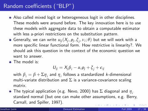
Random coe¢ cients (�BLP�)
Also called mixed logit or heterogeneous logit in other disciplines.These models were around before. The key innovation here is to usethese models with aggregate data to obtain a computable estimatorwith less a-priori restrictions on the substitution pattern.Generally, we can write uij (Xj , pj , ξ j , νi ; θ) but we will work with amore speci�c linear functional form. How restrictive is linearity?. Weshould ask this question in the context of the economic question wewant to answer.The model is:
Uij = Xjβi � αipj + ξ j + εij
with βi = β+ Σηi and ηi follows a standardized k-dimensionalmulti-variate distribution and Σ is a variance-covariance scalingmatrix.The typical application (e.g. Nevo, 2000) has Σ diagonal and ηistandard normal (but one can make other assumptions, e.g. Berry,Carnall, and Spiller, 1997).
Jonathan Levin (Economics 257 Stanford University)Demand Estimation Fall 2009 17 / 38

Random coe¢ cients (cont.)
In either case, with this we can write
Uij = δj + νij
such that δj = Xjβ� αpj + ξ j and νij = XjΣηi + εij .Now it is easy to see the di¤erence from the basic logit model: theidiosyncratic error term is not i.i.d but depends on the productcharacteristics, so consumers who like a certain product are morelikely to like similar products.How would the substitution matrix look now? Think about thederivatives:
�αsj (1� sj ) becomes �Zηi
αi sij (1� sij )dF (ηi )
αsj sk becomesZηi
αi sij sikdF (ηi )
This achieves exactly what we wanted: substitution which depends onthe characteristics (which characteristics?).
Jonathan Levin (Economics 257 Stanford University)Demand Estimation Fall 2009 18 / 38

Estimating random coe¢ cients
The key point that facilitates the estimation of this and relatedmodels is the inversion, i.e. the possibility to write δ(s) instead ofs(δ). If this can be done, then we can proceed relatively easy byapplying simple GMM restrictions.
In the previous models, this inversion was carried out analytically.Here that won�t work but we can invert numerically, conditional onthe �non-linear�parameters of the model, i.e. Σ. Once we have this,we can specify moment conditions. It is important to remember thatwe need enough moment conditions to identify the Σ parameters aswell.
Jonathan Levin (Economics 257 Stanford University)Demand Estimation Fall 2009 19 / 38

Estimating random coe¢ cients, cont.
Another problem here is that to compute the integral s(δ) we need torely on simulations. The idea: obtain draws from the distribution of
ηi and approximate the integralZηi
sijdF (ηi ) by1NS
NS
∑i=1sij (ηi ). The
trade-o¤ here is between more accurate approximation and increasedcomputation time.
Two computational notes:
We take the draws only once, in the beginning, otherwise we neverconverge.We do not need a whole lot of simulations per market; with manymarkets the simulation errors average out.
Jonathan Levin (Economics 257 Stanford University)Demand Estimation Fall 2009 20 / 38

Estimating random coe¢ cients (cont.)
The estimation algorithm (see also Nevo, 2000):1 Given (δ,Σ) compute s(δ,Σ) using the simulation draws (standardlogit per type), as described before.
2 Invert to get δ(s,Σ). This is done numerically by iterating over
δnew = δold + (ln so � ln s(δold ,Σ))
Berry shows that this is a contraction (need initial values for δ).3 Regular GMM of δ(s,Σ) on X , instrumenting for p, and using moremoment conditions to identify Σ as well. The search is donenumerically, with the added shortcut that the β�s enter linearly, so weneed to numerically search only over the non-linear parameters.
Note that the formulation has the dimension of β and of Σ the same. Thisis arti�cial and not necessary. The former enters the mean utility and thelatter enters the substitution pattern. Moreover, the main computationalburden is with respect to Σ, so this is where we really want to save onparameters. We can let β be quite rich without much cost.
Jonathan Levin (Economics 257 Stanford University)Demand Estimation Fall 2009 21 / 38

BLP (1995) Automobiles
Data on all models marketed 1971 to 1990: annual US sales data, carcharacteristics, Consumer Reports reliability ratings, miles per gallon.
Price variable is the list retail price (in $1000s) for the base model, in1983 dollars.
Market size is number of households in the US.
Speci�cations: simple logit, IV logit, BLP. Price instruments arefunctions of rival product characteristics and cost shifters.
Also incorporate a cost model:
p = mc + b (p, x , ξ; θ)
or rewriting with mc = exp(wγ+ω):
ln (p � b (p, x , ξ; θ)) = wγ+ω.
Jonathan Levin (Economics 257 Stanford University)Demand Estimation Fall 2009 22 / 38

BLP (1995) Automobiles, Results
Logit model: 1494 of 2217 models have inelastic demands -inconsistent with pro�t maximization. With IV, allows for unobservedproduct quality: only 22 models have inelastic demands.
Full model: most coe¢ cients at least somewhat plausible. Costs: ωaccounts for 22% of the estmate variance in log marginal cost.Correlation between ω and ξ is positive (why?).
Jonathan Levin (Economics 257 Stanford University)Demand Estimation Fall 2009 23 / 38

BLP (1995) Results
Jonathan Levin (Economics 257 Stanford University)Demand Estimation Fall 2009 24 / 38

BLP (1995) Results
Jonathan Levin (Economics 257 Stanford University)Demand Estimation Fall 2009 25 / 38

BLP (1995) Results
Jonathan Levin (Economics 257 Stanford University)Demand Estimation Fall 2009 26 / 38

Nevo (2000)
Ready-to-Eat (RTE) cereal market: highly concentrated, many similarproducts and yet apparently margins and pro�ts are relatively high.What is the source of market power? Di¤erentiation? Multi-product�rms? Collusion?Data: market is de�ned as a city-quarter. IRI data on market sharesand prices for each brand-city-quarter: 65 cities, 1Q88-4Q92. Focuson top 25 brands � total share is 43-62%.Most of the price variation is cross-brand (88.4%), the remainder ismostly cross-city, and a small amount is cross-quarter.Relatively poor �brand characteristics,� so model ξ j as brand ��xede¤ect�plus market-level �error term�. Fixed e¤ect speci�cationdi¤ers from random e¤ect set-up in BLP, and is possible because ofpanel data. Later project brand �xed e¤ect on characteristics.Instruments: price of same brand in other city. Identifying assumption:conditional on brand �xed e¤ect, covariation of prices across cities isdue to common cost shocks, not demand shocks. (plausible?)
Jonathan Levin (Economics 257 Stanford University)Demand Estimation Fall 2009 27 / 38

Nevo (2000)
Jonathan Levin (Economics 257 Stanford University)Demand Estimation Fall 2009 28 / 38

Nevo (2000)
Jonathan Levin (Economics 257 Stanford University)Demand Estimation Fall 2009 29 / 38

Nevo (2000)
Jonathan Levin (Economics 257 Stanford University)Demand Estimation Fall 2009 30 / 38

Nevo (2000)
Compares to accounting PCM as estimated by Cotterill (1996) andconcludes that multi-product Bertrand-Nash cannot be rejected.
Jonathan Levin (Economics 257 Stanford University)Demand Estimation Fall 2009 31 / 38

Consumer Stockpiling
Demand estimates for CPGs often use time-series variation in pricesthat comes from sales.
Problem: short-run and long-run elasticities may be very di¤erent ifthe response to a sale is to �stockpile� inventory at home. Thinkabout something like �cash-for-clunkers�� how much of the salesincrease was intertemporal substitution?
Example: suppose all the toilet paper at the supermarket is markeddown 50% for a week, and we observe a 20% increase in demand.This does not mean that if prices were permanently reduced 50% thatnational consumption of toilet paper would increase 20%!
Jonathan Levin (Economics 257 Stanford University)Demand Estimation Fall 2009 32 / 38

Consumer Stockpiling: Hendel & Nevo
Hendel and Nevo (2006, RJE): evidence for stockpiling, e.g. the�post-promotion dip�.
Hendel and Nevo�s (2006, EMA): dynamic demand model withconsumer inventory as an (unobserved) state variable. Estimate themodel using household-level scanner data on laundry detergents.Pretty complicated.
Hendel and Nevo (2009, WP): a �simpler�method based on aparticular model of inventory and sales behavior, that does not requireestimation of a complicated dynamic decision proces.
Jonathan Levin (Economics 257 Stanford University)Demand Estimation Fall 2009 33 / 38
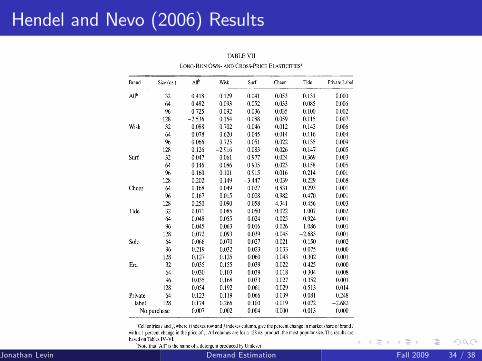
Hendel and Nevo (2006) Results
Jonathan Levin (Economics 257 Stanford University)Demand Estimation Fall 2009 34 / 38
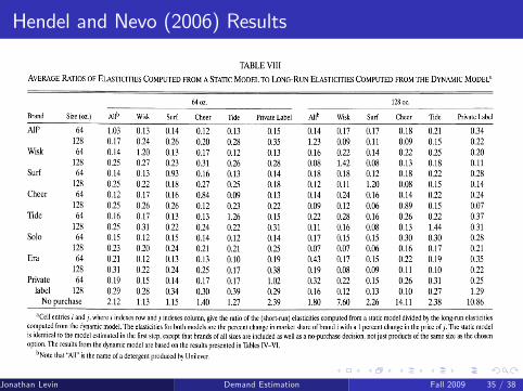
Hendel and Nevo (2006) Results
Jonathan Levin (Economics 257 Stanford University)Demand Estimation Fall 2009 35 / 38

Comments and extensions to logit-related models
1 So far we had in mind only aggregate data. How much better can wedo with individual-level data?
1 We can get �exible substitution patterns for free2 We may worry less about price endogeneity (why? why do we still needto worry about it?)
3 With panel dimension, we may be able to identify taste parameters forthe unobserved quality
(ref: Goldberg, 1995; �micro BLP�, 2004).
Jonathan Levin (Economics 257 Stanford University)Demand Estimation Fall 2009 36 / 38

Comments and extensions to logit-related models (cont.)
1 Instruments: most use instruments that are based on the exogeneityof the characteristics. As already discussed, this is questionable. Italso makes our counterfactuals unlikely to hold for the long run, ascharacteristics will respond.One can use the Hausman-type instruments (similar idea in Nevo,2001), but they have their issues. Optimally, we would like to havetrue product-speci�c cost shifters, but these are hard to �nd. Oncewe think about endogenous characteristics, this issue becomes moreexplicit.
Jonathan Levin (Economics 257 Stanford University)Demand Estimation Fall 2009 37 / 38

Comments and extensions to logit-related models (cont.)
3. Too many characteristics problem: any new product comes with anew dimension of unobserved tastes (εij ), and a new set of consumerswho really like it. Happens even if the new product is identical orinferior to existing products (eg red bus-blue bus).
This is likely to bias upwards estimates for markups, and to biasupwards welfare e¤ects of new goods.It does not allow us to use information on goods with zero marketshares; the model predicts positive shares.
One solution: Berry and Pakes, 2002. Like BLP but no εij . Tricky torecover the mean utility as a function of market shares because: (a)no smooth market share function: they use the vertical model for onecoe¢ cient (e.g. price), conditional on the other coe¢ cients; and (b)inversion is not a contraction anymore: they use numerical techniques.Another solution: Bajari and Benkard, 2005. Based on an hedonicapproach (and requires a �dense�product space).
Jonathan Levin (Economics 257 Stanford University)Demand Estimation Fall 2009 38 / 38


