34
Difference in Difference and Regression Discontinuity
| Date post: | 28-Dec-2015 |
| Category: |
Documents |
| Upload: | clifford-hensley |
| View: | 236 times |
| Download: | 0 times |
Difference in Difference and Regression Discontinuity
2
Review
• From Lecture I– Causality is difficult to Show from cross
sectional observational studies• What caused what?
– X caused Y, Y caused X
• Omitted Variable Bias/Confounding– In some cases you can say whether the estimate is an
upper-bound or lower bound estimate– Other times impossible to sign bias since omitted
variables bias the coefficient of interest positively and negatively. Net effect impossible to determine a-priori.
3
Review (cont.)
• Discussed Randomized Control Trials as a simple (but not necessarily practical) way to solve the causality problem
• Randomization works because we can be sure about temporal precedence
• Randomization works because treatment and control groups are balanced on observables and un-observables
4
Review (cont.)
• Also quickly presented some other commonly used research designs
• X 01 - Observe only data from post treatment (X)
• 01 X 02 – Observe data from pre and post treatment periods
• 01 02 X 03 – Observe data from pre and post treatment; observe a longer pre period
• Common Feature of all these designs is that there is NO CONTROL GROUP
5
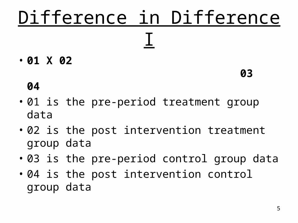
Difference in Difference I
• 01 X 02 03 04
• 01 is the pre-period treatment group data
• 02 is the post intervention treatment group data
• 03 is the pre-period control group data
• 04 is the post intervention control group data
6
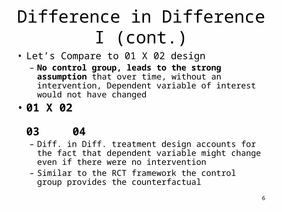
Difference in Difference I (cont.)
• Let’s Compare to 01 X 02 design– No control group, leads to the strong assumption
that over time, without an intervention, Dependent variable of interest would not have changed
• 01 X 02 03 04– Diff. in Diff. treatment design accounts for the fact that
dependent variable might change even if there were no intervention
– Similar to the RCT framework the control group provides the counterfactual
7
Difference in Difference I (cont.)
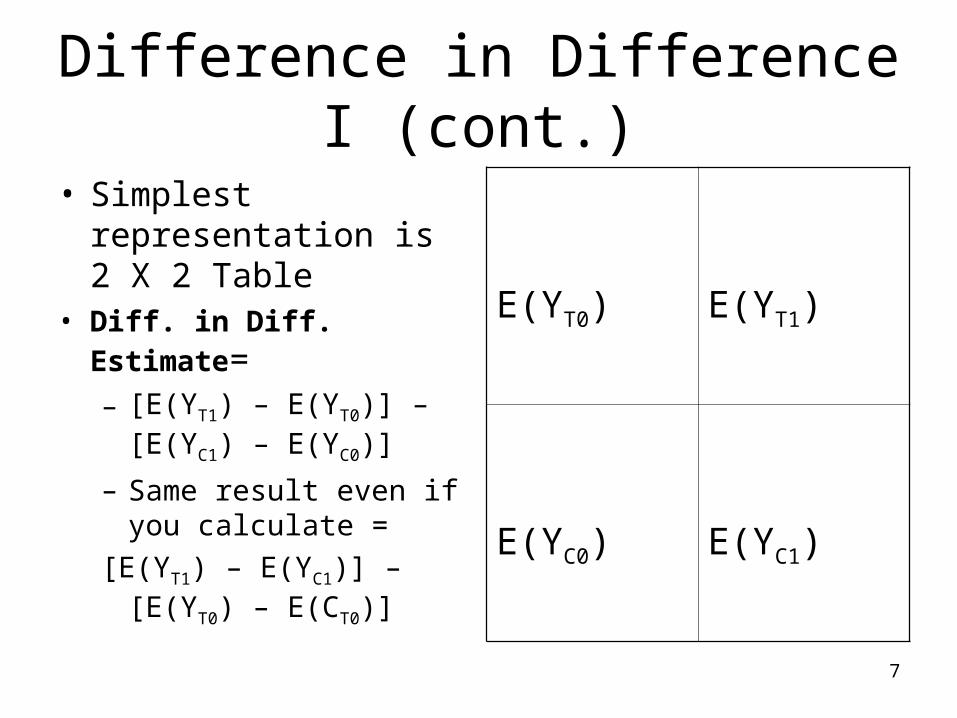
• Simplest representation is 2 X 2 Table
• Diff. in Diff. Estimate=– [E(YT1) – E(YT0)] –
[E(YC1) – E(YC0)]
– Same result even if you calculate =
[E(YT1) – E(YC1)] – [E(YT0) – E(CT0)]
E(YT0) E(YT1)
E(YC0) E(YC1)
8
Difference in Difference I (cont.)
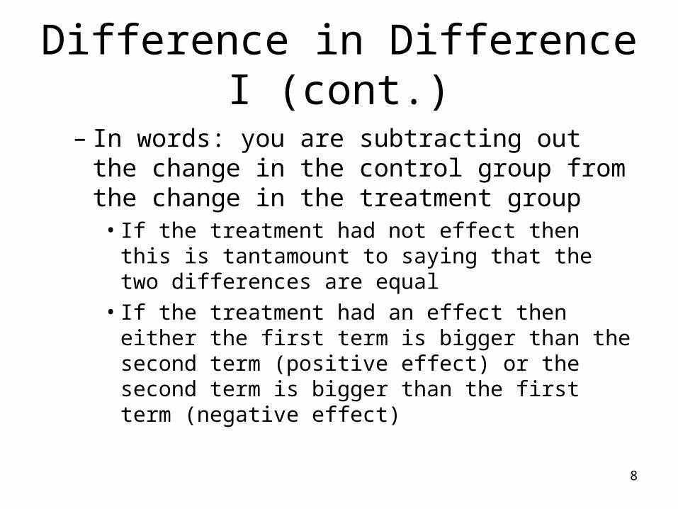
– In words: you are subtracting out the change in the control group from the change in the treatment group
• If the treatment had not effect then this is tantamount to saying that the two differences are equal
• If the treatment had an effect then either the first term is bigger than the second term (positive effect) or the second term is bigger than the first term (negative effect)

9
Difference in Difference II
• Why is Diff. and Diff. powerful?– MAIN REASON: We have a control group – Another problem with cross-sectional studies is that
we worry about unobserved and hard to measure differences between the treatment and control group
• In the difference in difference estimate, Unobserved differences across treatment and control that stay constant over time are differenced out
– Another way of saying this is that these unobserved unchanging characteristics effect the Level but not the changes
10
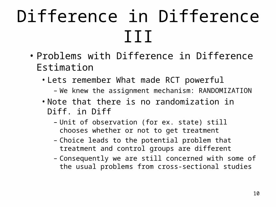
Difference in Difference III
• Problems with Difference in Difference Estimation
• Lets remember What made RCT powerful– We knew the assignment mechanism:
RANDOMIZATION
• Note that there is no randomization in Diff. in Diff– Unit of observation (for ex. state) still chooses whether or
not to get treatment– Choice leads to the potential problem that treatment and
control groups are different– Consequently we are still concerned with some of the
usual problems from cross-sectional studies
11
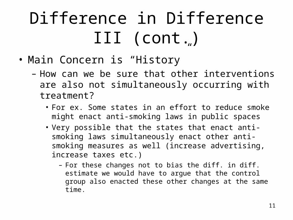
Difference in Difference III (cont.)
• Main Concern is “History”– How can we be sure that other interventions are also
not simultaneously occurring with treatment?• For ex. Some states in an effort to reduce smoke might enact
anti-smoking laws in public spaces• Very possible that the states that enact anti-smoking laws
simultaneously enact other anti-smoking measures as well (increase advertising, increase taxes etc.)
– For these changes not to bias the diff. in diff. estimate we would have to argue that the control group also enacted these other changes at the same time.
12
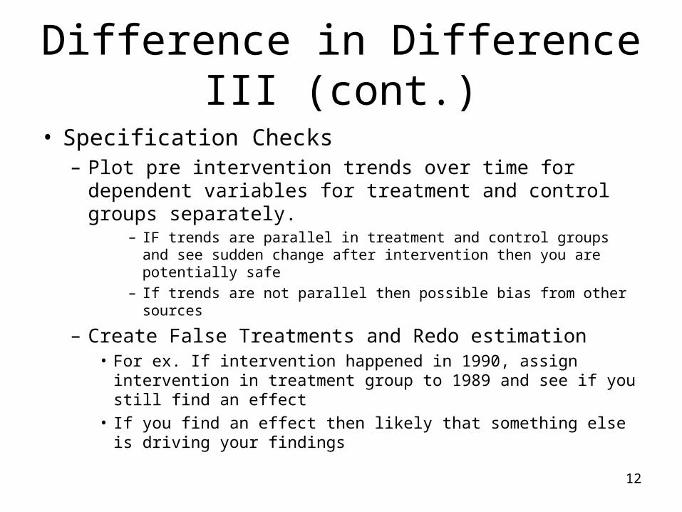
Difference in Difference III (cont.)
• Specification Checks– Plot pre intervention trends over time for dependent
variables for treatment and control groups separately.– IF trends are parallel in treatment and control groups and see
sudden change after intervention then you are potentially safe
– If trends are not parallel then possible bias from other sources
– Create False Treatments and Redo estimation• For ex. If intervention happened in 1990, assign intervention
in treatment group to 1989 and see if you still find an effect• If you find an effect then likely that something else is driving
your findings
13
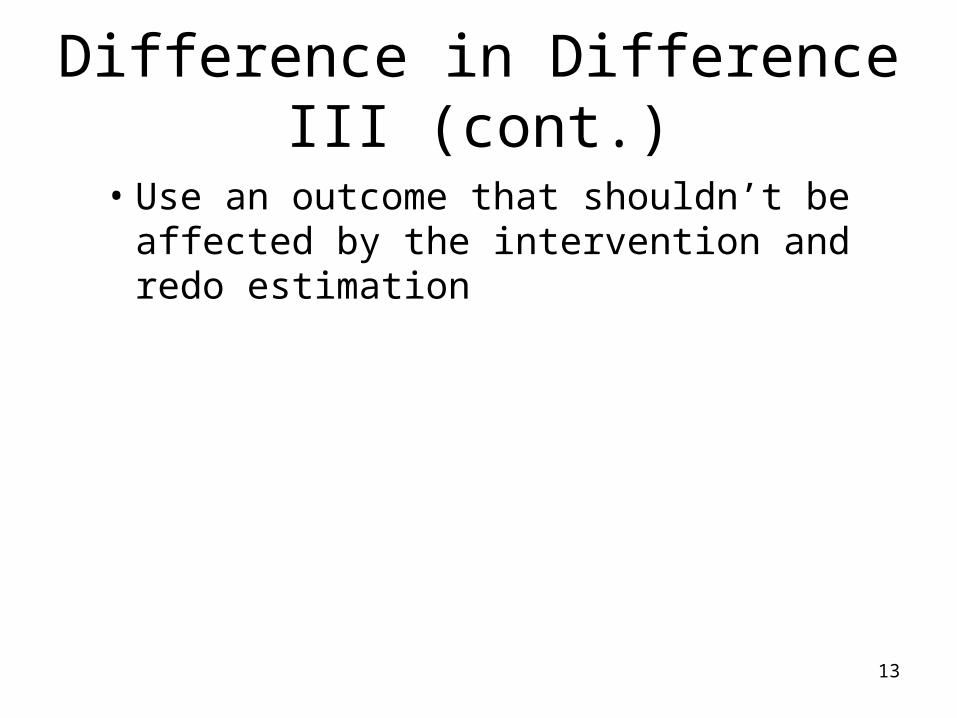
Difference in Difference III (cont.)
• Use an outcome that shouldn’t be affected by the intervention and redo estimation
14
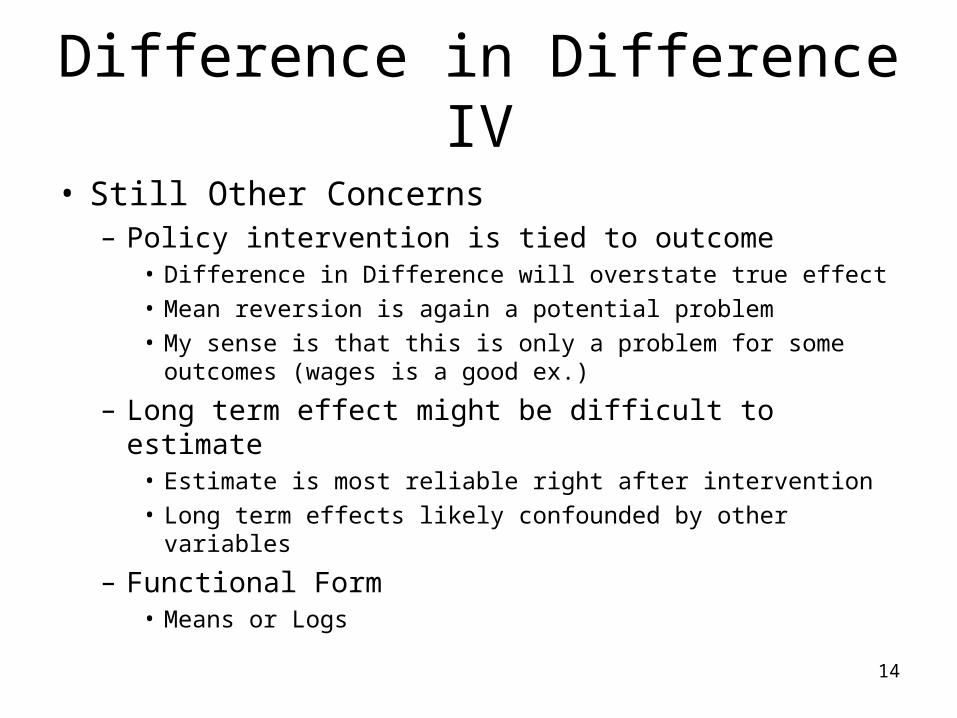
Difference in Difference IV
• Still Other Concerns– Policy intervention is tied to outcome
• Difference in Difference will overstate true effect• Mean reversion is again a potential problem• My sense is that this is only a problem for some outcomes
(wages is a good ex.)
– Long term effect might be difficult to estimate• Estimate is most reliable right after intervention• Long term effects likely confounded by other variables
– Functional Form• Means or Logs
15
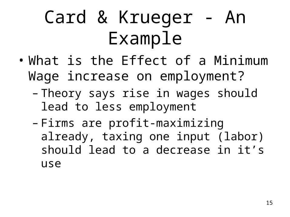
Card & Krueger - An Example
• What is the Effect of a Minimum Wage increase on employment? – Theory says rise in wages should lead to less
employment– Firms are profit-maximizing already, taxing
one input (labor) should lead to a decrease in it’s use
16
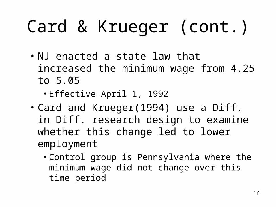
Card & Krueger (cont.)
• NJ enacted a state law that increased the minimum wage from 4.25 to 5.05
• Effective April 1, 1992
• Card and Krueger(1994) use a Diff. in Diff. research design to examine whether this change led to lower employment
• Control group is Pennsylvania where the minimum wage did not change over this time period
17
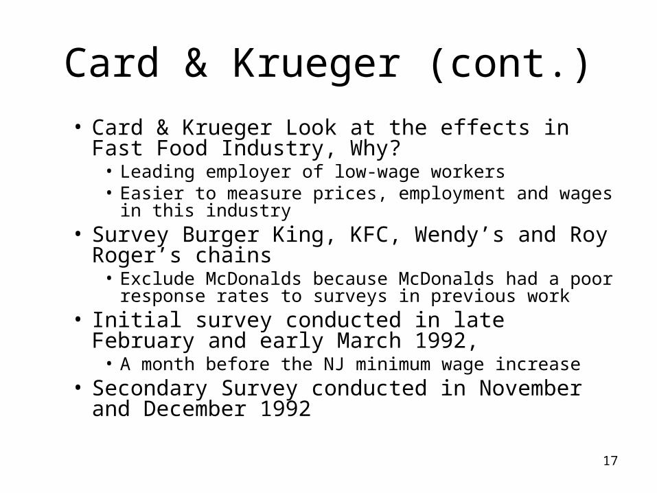
Card & Krueger (cont.)
• Card & Krueger Look at the effects in Fast Food Industry, Why?
• Leading employer of low-wage workers• Easier to measure prices, employment and wages in this
industry• Survey Burger King, KFC, Wendy’s and Roy Roger’s
chains• Exclude McDonalds because McDonalds had a poor
response rates to surveys in previous work • Initial survey conducted in late February and early
March 1992, • A month before the NJ minimum wage increase
• Secondary Survey conducted in November and December 1992

18
Card & Krueger (cont.)
• Around 80% response rate in pre-period– 90% of these 80% responded in post-period
• One Key question: Is the wage increase in N.J. meaningful?– Yes, average starting wage in New Jersey restaurants
increased by 10% (4.61 to 5.05)– In wave 1: 31% had a starting wage of 4.25
• In Pennsylvania, In wave 1, average starting wage in Pennsylvania was 4.63 and – In wage two there was no change
19
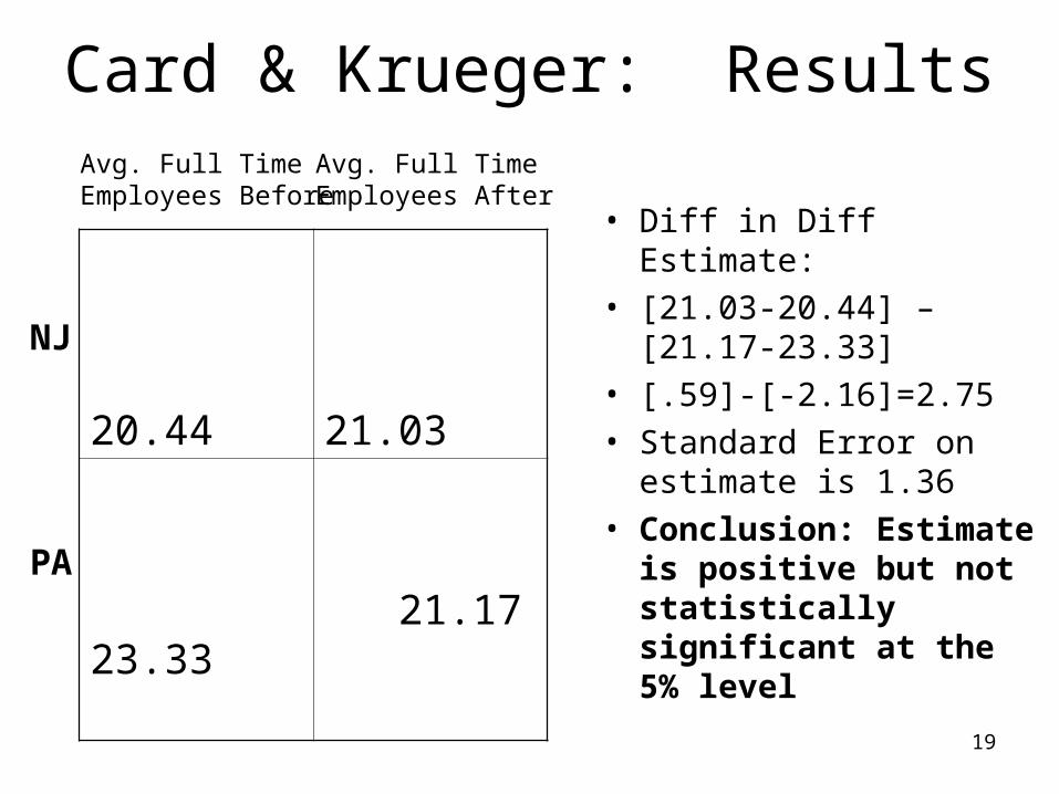
Card & Krueger: Results
20.44 21.03
23.33 21.17
• Diff in Diff Estimate:• [21.03-20.44] – [21.17-
23.33] • [.59]-[-2.16]=2.75• Standard Error on
estimate is 1.36• Conclusion: Estimate is
positive but not statistically significant at the 5% level
Avg. Full Time Employees Before
Avg. Full TimeEmployees After
NJ
PA
20
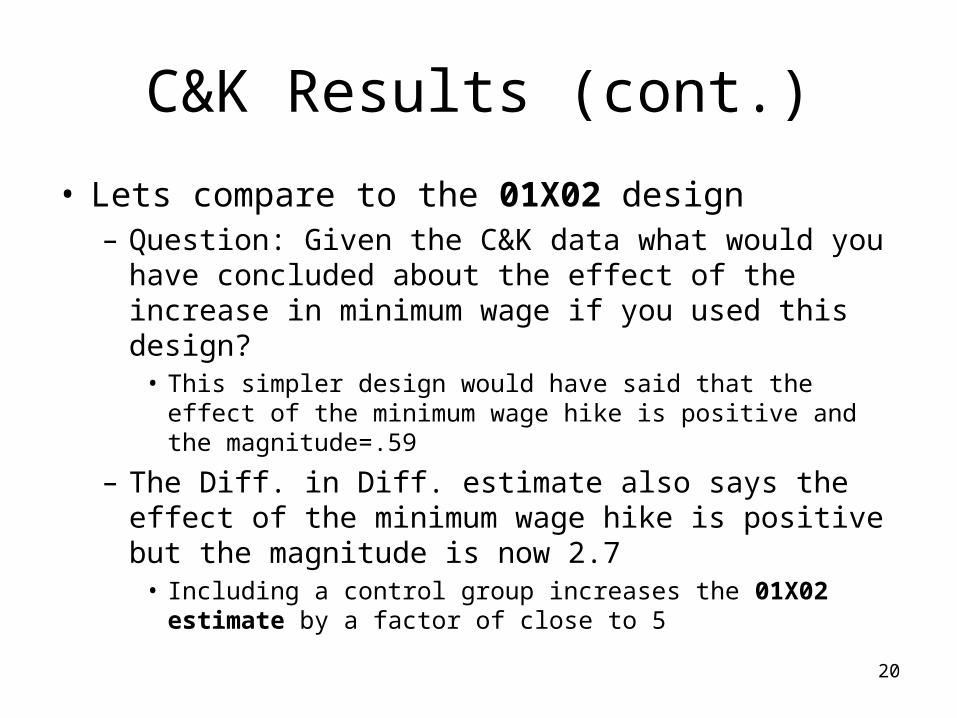
C&K Results (cont.)
• Lets compare to the 01X02 design– Question: Given the C&K data what would you have
concluded about the effect of the increase in minimum wage if you used this design?
• This simpler design would have said that the effect of the minimum wage hike is positive and the magnitude=.59
– The Diff. in Diff. estimate also says the effect of the minimum wage hike is positive but the magnitude is now 2.7
• Including a control group increases the 01X02 estimate by a factor of close to 5
21
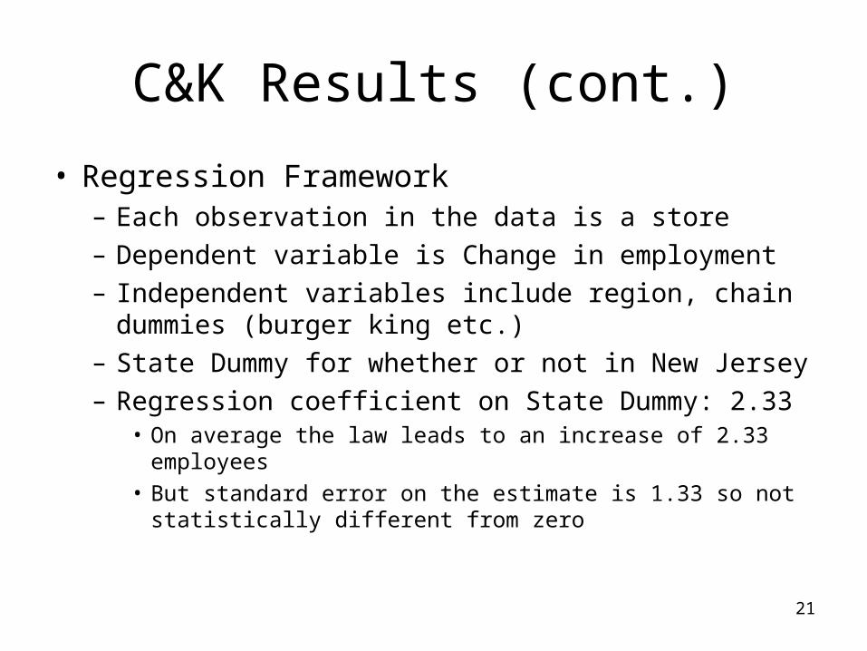
C&K Results (cont.)
• Regression Framework– Each observation in the data is a store– Dependent variable is Change in employment– Independent variables include region, chain dummies
(burger king etc.)– State Dummy for whether or not in New Jersey– Regression coefficient on State Dummy: 2.33
• On average the law leads to an increase of 2.33 employees• But standard error on the estimate is 1.33 so not statistically
different from zero
22
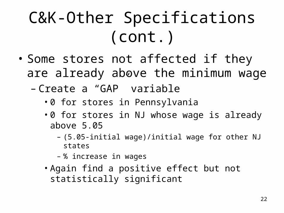
C&K-Other Specifications (cont.)
• Some stores not affected if they are already above the minimum wage– Create a “GAP” variable
• 0 for stores in Pennsylvania• 0 for stores in NJ whose wage is already above
5.05– (5.05-initial wage)/initial wage for other NJ states– % increase in wages
• Again find a positive effect but not statistically significant
23
C&K-Other Specifications (cont.)
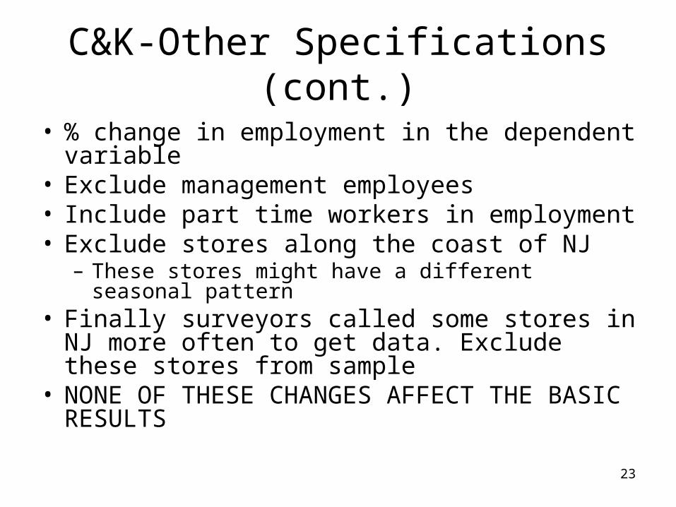
• % change in employment in the dependent variable
• Exclude management employees• Include part time workers in employment• Exclude stores along the coast of NJ
– These stores might have a different seasonal pattern• Finally surveyors called some stores in NJ more
often to get data. Exclude these stores from sample
• NONE OF THESE CHANGES AFFECT THE BASIC RESULTS
24
C&K - Other Specifications (cont.)
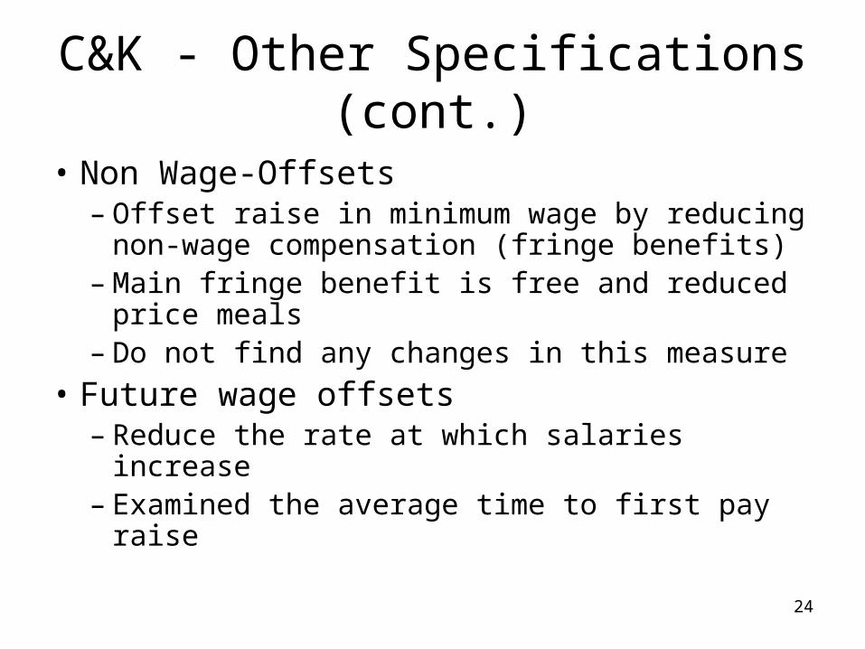
• Non Wage-Offsets– Offset raise in minimum wage by reducing
non-wage compensation (fringe benefits)– Main fringe benefit is free and reduced price
meals– Do not find any changes in this measure
• Future wage offsets– Reduce the rate at which salaries increase– Examined the average time to first pay raise
25
Regression Discontinuity
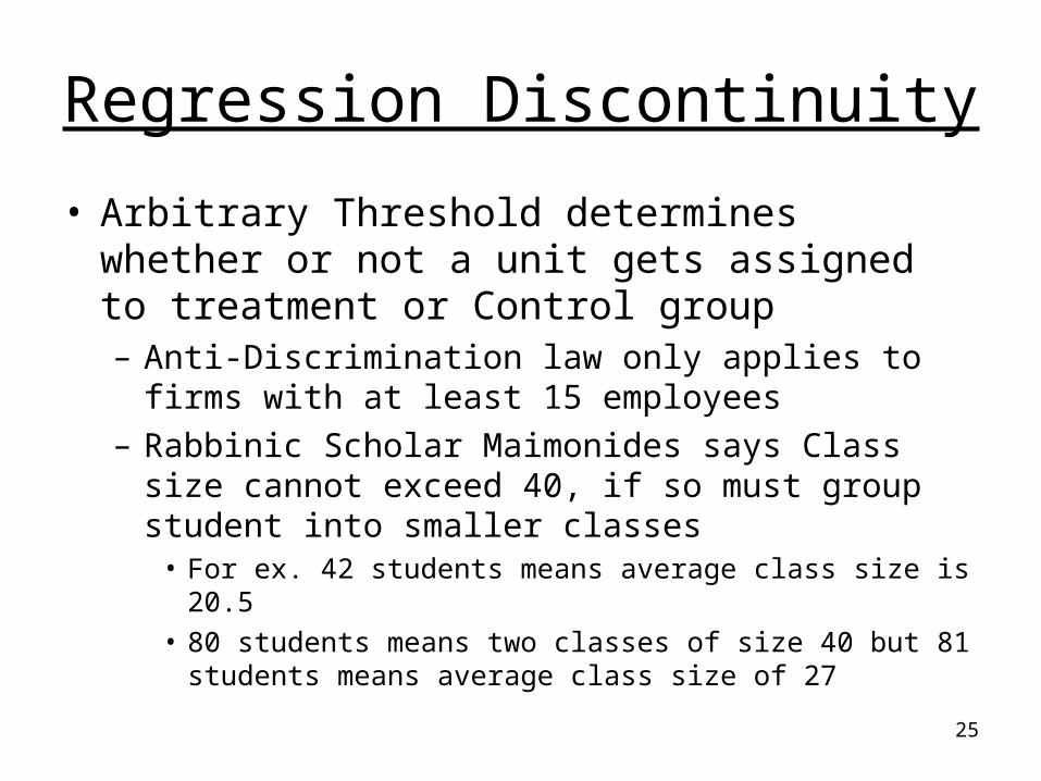
• Arbitrary Threshold determines whether or not a unit gets assigned to treatment or Control group– Anti-Discrimination law only applies to firms with at
least 15 employees– Rabbinic Scholar Maimonides says Class size cannot
exceed 40, if so must group student into smaller classes
• For ex. 42 students means average class size is 20.5• 80 students means two classes of size 40 but 81 students
means average class size of 27
26
Regression Discontinuity (cont.)
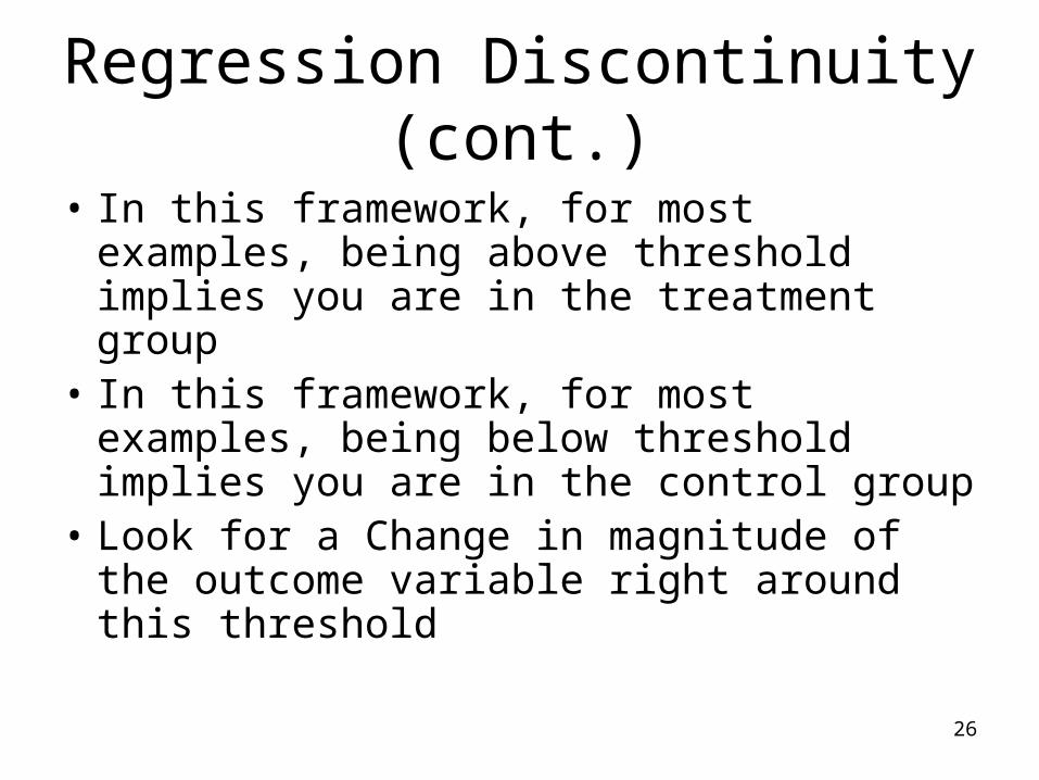
• In this framework, for most examples, being above threshold implies you are in the treatment group
• In this framework, for most examples, being below threshold implies you are in the control group
• Look for a Change in magnitude of the outcome variable right around this threshold

27
28
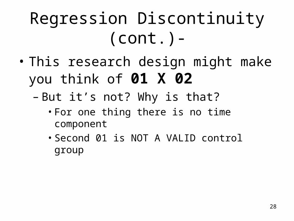
Regression Discontinuity (cont.)-
• This research design might make you think of 01 X 02– But it’s not? Why is that?
• For one thing there is no time component• Second 01 is NOT A VALID control group
29
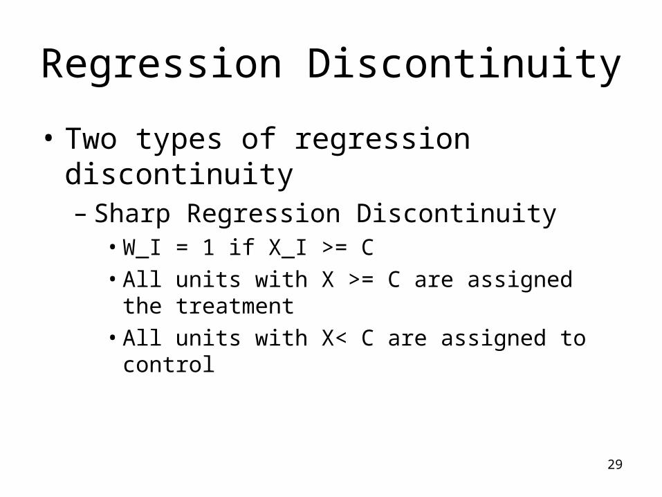
Regression Discontinuity
• Two types of regression discontinuity– Sharp Regression Discontinuity
• W_I = 1 if X_I >= C• All units with X >= C are assigned the treatment• All units with X< C are assigned to control
30
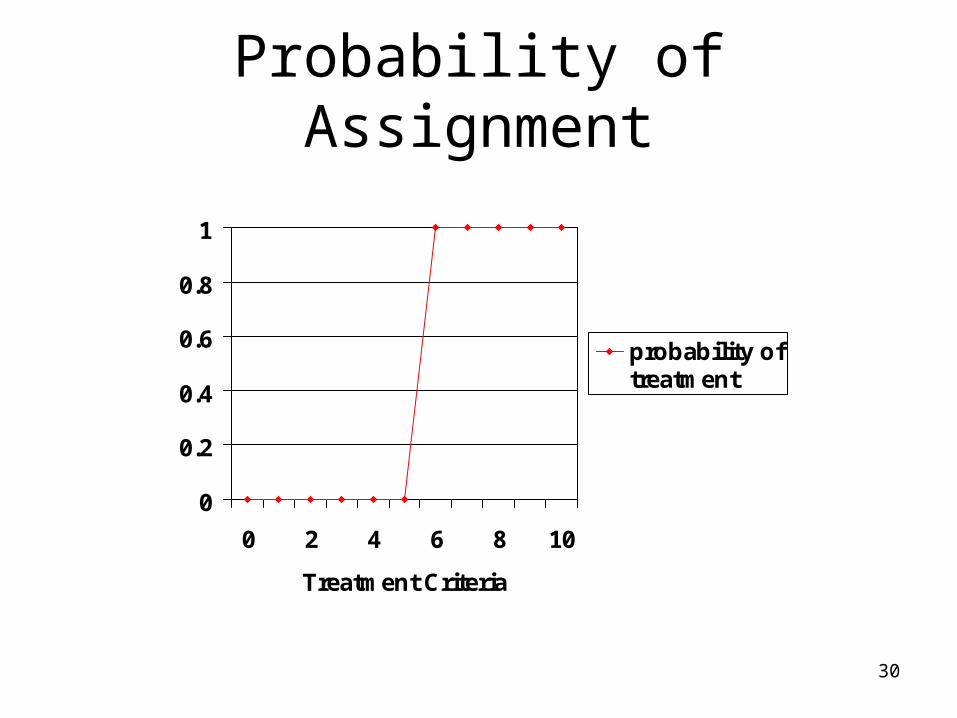
Probability of Assignment
0
0.2
0.4
0.6
0.8
1
0 2 4 6 8 10
Treatment Criteria
probability oftreatment
31
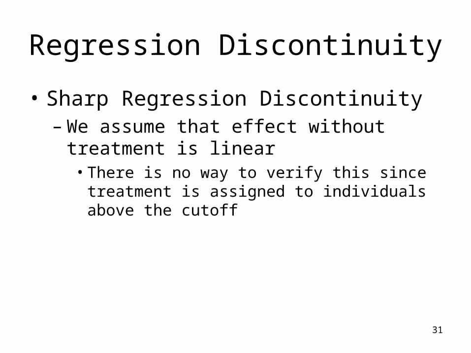
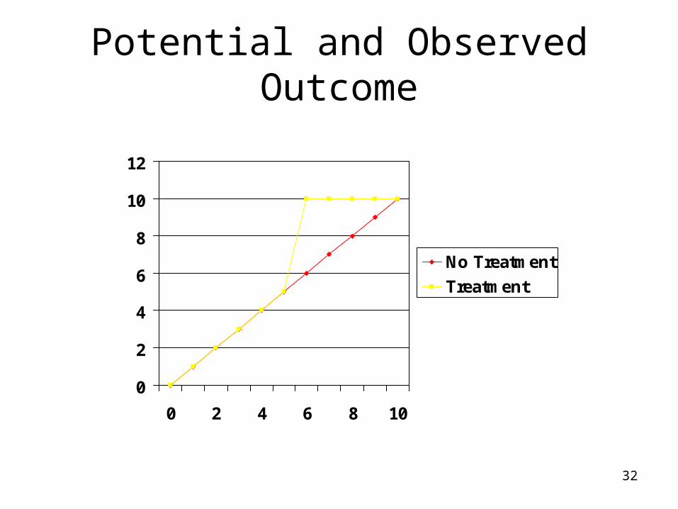
Regression Discontinuity
• Sharp Regression Discontinuity– We assume that effect without treatment is
linear• There is no way to verify this since treatment is
assigned to individuals above the cutoff
32
Potential and Observed Outcome
0
2
4
6
8
10
12
0 2 4 6 8 10
No Treatment
Treatment
33
Regression Discontinuity
• Fuzzy Regression Discontinuity Design• Probability of receiving does not have to be 1 at
the threshold• For ex. Individuals above some threshold could be
offered a treatment• The offer does not lead all individuals to take up
treatment• As an example think of a voucher scheme that
allows people to move neighborhoods. – For some individuals voucher amount is not enough to
get them to comply

34


