AN IMPLICIT RUNGE-KUTTA METHOD FOR INTEGRATION OF

DIFFERENTIAL-ALGEBRAIC EQUATIONS OF MULTIBODY DYNAMICS

Dan Negrut Mechanical Dynamics, Inc.

Edward J. Haug

The University of Iowa

Horatiu C. German The University of Iowa

This paper has not been submitted elsewhere in identical or similar form, nor will it be during

the first three months after its submission to Multibody System Dynamics. Abstract. When performing dynamic analysis of a constrained mechanical system, a set of index 3

differential algebraic equations (DAE) describes the time evolution of the model. This paper presents a

state space DAE solution framework that can embed an arbitrary implicit ordinary differential equations

(ODE) code for numerical integration of a reduced set of state space ordinary differential equations. This

solution framework is constructed with the goal of leveraging with minimal effort established off the shelve

implicit ODE integrators for efficiently solving the DAE of multibody dynamics. This concept is

demonstrated by embedding a well-known public domain singly diagonal implicit Runge-Kutta code in the

framework provided. The resulting L-stable, stiffly accurate implicit algorithm is shown to be two orders

of magnitude faster than a state of the art explicit algorithm when used to simulate a stiff vehicle model.

Keywords: implicit integration, index 3 DAE, state-space form, singly diagonal implicit Runge-

Kutta formula, coordinate partitioning

1. Introduction. This Section introduces the equations that govern the time evolution of a

mechanical system; i.e., the index 3 differential-algebraic equations (DAE) for multibody

dynamics, along with a brief overview of numerical methods for their solution. Section 2

2

presents the DAE reduction process into state-space ordinary differential equations (SSODE)

through the generalized coordinate partitioning method [32]. Section 3 presents the proposed

solution method, along with a detailed discussion regarding the computation of Jacobian

information required for implicit integration of the SSODE. Based on the method of Section 3, a

singly diagonal implicit Runge-Kutta (SDIRK) algorithm is introduced in Section 4. In Section 5,

numerical experiments for two stiff mechanical systems are presented. The test problems are

used to validate the proposed algorithm and to compare its efficiency with the performance of an

explicit integrator. Section 6 presents conclusions of the study.

The state of a multibody system at the position level is represented by a vector

[ ]1 , ..., T

nq qq = of generalized coordinates. The velocity of the system is described by the array

[ ]1 , ..., T

nq qq = of generalized velocities. Given the quantities q and q , the position and velocity

of each body in the system are uniquely determined. There are numerous ways in which

generalized coordinates and velocities can be selected [9, 17]. The generalized coordinates used

in this paper are Cartesian coordinates for position and Euler parameters for orientation of body

centroidal reference frames. Thus, the position of body i is described by the vector

[ ], , T

i i i ix y z=r , while the orientation of body i is given by the vector [ ]0 1 2 3, , , Ti i i i ie e e e=e of

Euler parameters [17], which must satisfy the normalization condition 1Ti i =e e . Consequently,

for a mechanical system containing bn bodies, the composite vector of generalized coordinates is

71 1 ... b

T nT T T Tnb nb= ∈ q r e r e (1)

When compared with the alternative of using a set of relative generalized coordinates, the

Cartesian coordinates considered here are convenient, because of the rather complex expression

for the Jacobian associated with the implicit integration of the SSODE.

In any constrained mechanical system, joints connecting bodies restrict their relative motion

and impose constraints on the generalized coordinates. To simplify the presentation, only

3

holonomic and scleronomic constraints are considered; i.e., constraints characterized by algebraic

equations involving generalized coordinates,

( ) ( ) ( )[ ]1 ...T

m= Φ Φ =Φ q q q 0 (2)

where m is the total number of constraint equations that must be satisfied by the generalized

coordinates throughout the simulation, including the Euler parameter normalization condition for

each body. It is assumed here that the m constraint equations are independent. The number of

degrees of freedom ndof is thus the difference between the number of generalized coordinates and

the number of constraints; i.e., ndof n m= − .

Differentiating Eq. (2) with respect to time leads to the velocity kinematic constraint

equation,

( ) =qΦ q q 0 (3)

where over dot denotes differentiation with respect to time and subscript denotes partial

differentiation; i.e., i

j

∂Φ

∂Φ=

qΦ is an 7 bm n× matrix. The acceleration kinematic constraint

equations are obtained by differentiating Eq. (3) with respect to time,

( ) ( )( ) ( ),= − ≡q q qΦ q q Φ q q q τ q q (4)

Equations (2)-(4) characterize the admissible motion of the mechanical system.

The state of the mechanical system changes in time under the influence of applied forces.

The time evolution of the system is governed by the Lagrange multiplier form of the constrained

equations of motion [17],

( ) ( ) ( )A , ,T t+ =qM q q Φ q λ Q q q (5)

where ( ) n nM q ×∈ is the symmetric system mass matrix, m∈λ is the array of Lagrange

multipliers that account for workless constraint forces, and ( )A , , nt ∈Q q q is the generalized

applied force vector.

4

Equations (2)-(5) comprise a system of DAE. It is known that DAE are not ordinary

differential equations (ODE) [25]. Analytical solutions of Eqs. (2) and (5) automatically satisfy

Eqs. (3) and (4), but this is not true for numerical solutions. In general, the task of obtaining a

numerical solution of the DAE of Eqs. (2)-(5) is substantially more difficult and prone to intense

numerical computation than that of solving ODE. In this context, a number of numerical methods

have been developed for the solution of the DAE of multibody dynamics. Most of these methods

belong to one of the following categories: (1) stabilization methods; (2) projection methods; (3)

state space methods.

Early stabilization-based numerical algorithms are based on the so called constraint

stabilization technique [6]. The original DAE is reduced to index 1 [16, 17] by considering the

integration of Eqs. (4) and (5), instead of Eqs. (2) and (5). Since after direct integration the

constraints of Eq. (2) fail to be satisfied, the right side of the acceleration kinematic constraint

equation is modified to take into account the constraint violation. The right side of the

acceleration kinematic constraint equation is thus altered to

2α β= − −τ τ Φ Φ (6)

The last two terms of Eq. (6) do not appear in the original form of acceleration kinematic

constraint equation of Eq. (4). They are introduced to compensate for errors in satisfying

constraint equations at position and velocity levels. The process of optimally choosing the

parameters α and β is problematic and is yet to be resolved [2, 24].

Several stabilization algorithms [2] have as starting point the underlying ODE associated with

the index 3 DAE of multibody dynamics, which is obtained by formally eliminating the Lagrange

multipliers from the equations of motion of Eq. (5). Using Eqs. (4) and (5),

1 1 1 A( ) [ ]T− − −= −q q qλ Φ M Φ Φ M Q τ (7)

5

The Lagrange multipliers are then substituted back into Eq. (5) to obtain the underlying ODE

associated to the DAE, which theoretically, can be further transformed to a first order system of

ODE,

ˆ( )=z f z (8)

with TT T ≡ z q q . By directly integrating the set of second order ODE, the kinematic

constraint equations at position and velocity levels will cease to be satisfied. In the spirit of

Baumgarte’s technique, a more general constraint stabilization term is added to the right side of

Eq. (8), to obtain [2]

ˆ( ) γ ( ) ( )= −z f z F z h z (9)

where γ 0> is a parameter, ( )F z is a 2 2n m× matrix, and

( )

( ) = q

Φ qh z

Φ q (10)

are the kinematic constraint expressions at position and velocity levels. The central issue is how

to choose the matrix ( )F z . Several choices are suggested in Ref. 2, which lead to good

algorithms for non-stiff and highly oscillatory problems. Details about the choice of the matrix

( )F z and the stability range for the parameter γ can be found in Ref. 2, 3, and 4.

A second class of algorithms for the numerical solution of the DAE of multibody dynamics is

based on so called projection techniques [10], in which all generalized coordinates are integrated

at each time step. Additional multipliers are introduced to account for the requirement that the

solution satisfy constraint equations at position, velocity, and in some formulations, acceleration

levels. In Ref. 14, the DAE is reduced to an analytically equivalent index 2 problem, in which

projection is only performed at the velocity level. An extra multiplier µ is introduced to insure

that the velocity kinematic constraint equation of Eq. (3) is also satisfied. The algorithm uses a

backward differentiation formula (BDF) to discretize the following form of the equations of

motion:

6

A

( )

( ) ( )

( )( )

T

T

= −

= −

=

=

q

q

q

q v Φ q µ

M q v Q Φ q λ

Φ q 0Φ q q 0

(11)

In a similar approach [12], the DAE is reduced to index 1 and an additional multiplier η is

introduced, along with the requirement that the acceleration kinematic equation of Eq. (4) is

satisfied. In an analytical framework, all additional multipliers can be proved to be zero for the

actual solution. However, under discretization, these multipliers assume nonzero values, due to

truncation errors of the integration formula being used.

Starting from the index 1 formulation of Eqs. (4) and (5), an algorithm with no extra

multipliers is proposed in Ref. 12. All variables are integrated, and the kinematic constraint

equations at position, velocity, and acceleration levels are imposed. Under discretization, an

over-determined set of 2 3n m+ nonlinear equations in 2n m+ unknowns must be solved at each

integration step. Because of truncation errors, the equations become inconsistent and can only be

solved in a generalized sense. While in the case of linear constraint equations, the so-called ssf-

solution obtained using a special oblique projection technique is equivalent to that obtained by

integrating the state-space form using the same discretization formula, this ceases to be the case

in general [27]. The resulting method is robust, and it is comparable in terms of efficiency to the

index 1 formulation with additional multipliers.

The methods proposed in Ref. 12 and 14 belong to the class of so called derivative projection

methods; i.e., expressions for derivatives are modified by additional multipliers that ensure

constraint satisfaction. A second projection technique is based on the coordinate projection

approach. The derivatives are no longer modified, and integration is carried out to obtain a

solution of the index 1, or for some formulations index 2 DAE. Since all variables are integrated,

they do not satisfy the constraint equations, so some form of coordinate projection technique is

employed to bring the ODE solution to the constraint manifold [7, 11, 20, 30].

7

From a physical standpoint, the projection stage is conventional, and typically the underlying

ODE is integrated with very high accuracy to reduce the weight of the projection stage in the

overall algorithm. The code MEXX [21] for integration of multibody systems is based on

coordinate projection and uses relatively expensive but very accurate extrapolation methods for

integration of the ODE.

Another class of algorithms for DAE solution is based on the state-space reduction method.

The DAE is reduced to an equivalent ODE, using a local parameterization of the constraint

manifold. The dimension of this equivalent SSODE is reduced to ndof n m= − . This method

has the potential of using well established theory and reliable numerical techniques for the

solution the SSODE, which is an aspect that the algorithm proposed in this paper leverages.

Since constraint equations in multibody dynamics are generally nonlinear, a parameterization

of the constraint manifold can only be determined locally. Computational overhead results each

time the parameterization is changed. Non-linearity also leads to computational effort in

retrieving dependent generalized coordinates through the parameterization. This stage requires

the solution of a system of nonlinear equations, for which Newton-like methods are generally

used.

The choice of constraint parameterization differentiates among algorithms in this class. The

most used parameterization is based on an independent subset of position coordinates of the

mechanical system [32]. The partition of variables into dependent and independent sets is based

on an LU factorization with column pivoting of the constraint Jacobian matrix. This partition is

maintained as long as the dependent sub-Jacobian matrix (the derivative of the constraint

equations with respect to dependent coordinates) is not ill conditioned. The method has been

used extensively with large scale applications in multibody dynamics and has proved to be

reliable and accurate. This approach is presented in detail in Section 2.

Applying state-space methods for the solution of the DAE of multibody dynamics has been

subjected to critique in two aspects. First, the choice of projection subspace is generally not

8

global. Second, bad choices of the projection space result in SSODE that are demanding in terms

of numerical treatment, mainly at the expense of overall efficiency of the algorithm [1]. The

latter concern is addressed by the tangent-plane parameterization method [22], for which the

parameterization variables are obtained as linear combinations of generalized coordinates using

an SVD decomposition of the constraint Jacobian. The benefits of this reduction are anticipated

to be twofold. The resulting SSODE is expected to be numerically better conditioned and allow

for significantly larger integration step-sizes. Second, dependent variable recovery can take

advantage of information generated during state-space reduction. Finally, note that the state-space

based reduction alternatives presented above are particular cases of a more general framework

that is succinctly presented in Ref. 26.

The last state-space type method to be mentioned is the differentiable null space method [19].

It reduces the DAE to an equivalent SSODE by projecting the equations of motion onto the

tangent hyperplane of the manifold. The projection is done before discretization, and Lagrange

multipliers are eliminated from the problem. The algorithm requires a set of ndof vectors that

span the constraint manifold hyperplane, along with their first time derivative. The Gram-

Schmidt factorization method [5] is used to obtain this information. The algorithm is efficient

and robust, the resultant SSODE of dimension ndof being well conditioned. The

implementation of an implicit formula to integrate the resulting state-space ODE is difficult,

because of the Gram-Schmidt process embedded in the algorithm.

2. General Considerations Regarding the Coordinate Partitioning Method. The

coordinate partitioning method is a state space method that uses a subset of the generalized

coordinates to locally parameterize the constraint manifold. The vector of generalized

coordinates used for parameterization is denoted by ndof∈v , while the vector containing the

remaining m generalized coordinates is denoted by m∈u . Note that ndof m n+ = . The

9

partitioning of n∈q into v and u is done such that the sub-Jacobian of the constraint vector

function with respect to u is nonsingular; i.e.,

( )( )det 0≠uΦ q (12)

This generalized coordinate partitioning strategy is possible as long as the constraint

equations of Eq. (2) are independent [17]; i.e., as long as the constraint Jacobian qΦ has full row

rank.

Based on this partitioning, Eqs. (2)-(5) can be rewritten in the associated partitioned form

[23]

( ) ( ) ( ) ( )T+ + =vv vu vvM u, v v M u, v u Φ u, v λ Q u, v,u, v (13)

( ) ( ) ( ) ( )T+ + =uv uu uuM u, v v M u, v u Φ u, v λ Q u, v,u, v (14)

( ) =Φ u, v 0 (15)

( ) ( )+u vΦ u, v u Φ u, v v = 0 (16)

( ) ( ) ( )+u vΦ u, v u Φ u, v v = τ u, v,u, v (17)

The condition of Eq. (12) and the implicit function theorem [8] guarantee that, based on Eq.

(15), u can be represented locally as a function of v ,

( )u = h v (18)

where the function ( )h v has as many continuous derivatives as does the constraint function

( )Φ q .

With this, the system of DAE in Eqs. (13), (14), and (17) is reduced to a set of state-space

ordinary differential equations (SSODE), through a sequence of steps that use information

provided by Eqs. (16) and (18). Thus, since the coefficient matrix of u in Eq. (16) is

nonsingular, u can be determined as a function of v and v , where Eq. (18) is used to eliminate

explicit dependence on u . Next, Eq. (17) uniquely determines u as a function of v , v , and v ,

10

where results from Eqs. (16) and (18) are substituted. Since the coefficient matrix of λ in Eq.

(14) is nonsingular, λ can be determined uniquely as a function of v , v , and v , using

previously derived results. Finally, each of the preceding results may be substituted into Eq. (13)

to obtain the SSODE in the independent generalized coordinates v , [17],

( ) ( )ˆˆ t=M v v Q , v, v (19)

where

( )1 1 1ˆ TT− − −= − − − vv vu uv uu

u v v u u vM M M Φ Φ Φ Φ M M Φ Φ (20)

( )1 1 1ˆ TT− − −= − − − v vu u uu

u v u uQ Q M Φ τ Φ Φ Q M Φ τ (21)

The SSODE of Eq. (19) is well defined, since M̂ is positive definite [23].

3. Proposed Method. Since the coefficient matrix M̂ in Eq. (19) is positive definite, this

set of second order differential equations can be theoretically expressed in the form

( , , )t=v f v v (22)

where 1 ˆˆ −≡f M Q . The objective of this paper is to define a framework in which the solution of

the SSODE of Eq. (22) may be determined using an implicit ODE integrator. The goal is that the

framework is general enough to support, with minor adjustments, a diverse family of off-the-shelf

implicit ODE integrators. For this purpose, the second order SSODE is transformed into a first

order ODE,

( , )t=w g w (23)

where

TT T = w v v (24)

and

( , )( , , )

tt

=

vg w

f v v (25)

11

Implicit numerical integration of the ODE of Eq. (23) requires the ability to perform function

evaluation for ( ),tg w in Eq. (25), and to compute appropriate Jacobian information for the

solution of the non-linear algebraic equations obtained after the discretization of the ODE. Thus,

for a given v and v , evaluation of ( ),tg w is equivalent to computing the corresponding

acceleration v ; i.e., a solution of the linear system of equations of Eqs. (4) and (5). The Jacobian

is

≡ v v

0 IG

f f (26)

where I is the identity matrix of dimension ndof. To compute G, derivatives of the right side of

the differential equation of Eq. (22) must be provided; i.e., 1 ≡ vJ f and 2 ≡ vJ f are required. The

subset of equations of motion of Eq. (13) is differentiated with respect to independent position

and velocity coordinates to compute 1J and 2J , respectively. Differentiating Eq. (13) with

respect to v yields

( ) ( ) ( ) ( )( ) ( )

1

T T T

+ + + + +

+ + + = + +

vv vv vv vv vu vuv v vv u v u

v v vv v v v v v u v u vv u

M J M v M v u M u M u M u u

Φ Φ Φ u Q Q u Q uλ λ λ (27)

The quantities vu , vu , vu , and vλ are obtained by taking partial derivatives with respect to v of

Eqs. (15), (16), (17), and (14), respectively. This is an exercise in the chain rule differentiation

that yields [23],

1−= ≡−v u vu Φ Φ H (28)

( ) ( )1− = − + ≡ v u q qv uu Φ Φ q Φ q H J (29)

1= +vu HJ L (30)

( ) ( )-11

T= − + + uv uu

v uλ Φ R M M H J (31)

where

12

{ }1 [ ( ) ] ( )−= − + + −u u q u v u q vL Φ τ Φ q H τ τ J Φ q (32)

[( ) ( ) ] -

( ) ( )

T

T

=

+ + +

+ − −u u u uu u u u v u

u uuu v v

R M q Φ λ Q H Q Q J

Φ M q M Lλ (33)

The linear system that is obtained after substitution of these quantities into Eq. (27) is

( ) ( )

( ) ( )1

ˆ

T T= + + − + + +

+ + + +

v v v vu Tv u u v vu v

vv vu vv vuv u

MJ Q Q H Q J M L H R Φ λ H Φ λ

M v M u M v M u H (34)

Since the coefficient matrix M̂ in this multiple right side linear system is positive definite, Eq.

(34) uniquely defines 1J .

Computation of 2 = vJ v follows the steps taken for the computation of 1J . Taking the

derivative of Eq. (13) with respect to v yields

2T+ + = +vv vu v v

v v v u v vM J M u Φ λ Q u Q (35)

All derivatives in this expression are available, except the quantities 2J , vu , vu , and vλ . The

last three derivatives are obtained by taking partial derivatives with respect to v of Eqs. (16),

(17), and (14). By repeatedly applying the chain rule of differentiation, these derivatives are

obtained as

vu = H (36)

2+vu = N HJ (37)

( ) 2T−= + − − +

u u uu uv uuv u u vλ Φ Q H Q M N M M H J (38)

where

( )T−= +u u vN Φ τ H τ (39)

Substituting these results into Eq. (35), 2J is obtained as the solution of the multiple right side

system of linear equations,

13

2ˆ T= −MJ W H X (40)

where

= + −v v vuu vW Q H Q M N

( )= − + −u u uuu vX Q H Q M N

With this, the use of an implicit integrator only requires support for function evaluation and

Jacobian computation. Limiting the discussion to the family of diagonal implicit Runge-Kutta

[16] and BDF multistep methods [13], the configuration w at each stage or time step is corrected

by ∆w , where this correction is the solution of a linear system of the form

( α )− =I G ∆w err (41)

where err is the residual in satisfying the integration formula for a multi-step method, or the

stage equation for a Runge-Kutta method; α γh≡ is a coefficient that depends on the integration

step-size h and an integration-formula specific coefficient γ ; and I is the identity matrix of

dimension 2 .ndof×

When solving Eq. (41), advantage can be taken of the special structure of G. Thus, with

1 2[ ]T T T≡err b b , the vector [ ]T T T≡∆w ∆v ∆v is the solution of the linear system

1

1 2 2

αα α

−=

− −

I I b∆vJ I J b∆v

where I is the identity matrix of dimension ndof. The solution of this system can be obtained by

solving two linear systems of dimension ndof for the corrections ∆v and ∆v . The correction

∆v is obtained as the solution of

( )22 1 1 2 2 1α α α α− − = + −I J J ∆v b b J b (42)

whereas the correction ∆v is obtained by solving

( )22 1 2 1 1α α α− − = +I J J v b J b∆ (43)

14

Savings in CPU time are obtained if, instead of solving these systems, Eqs. (42) and (43) are

multiplied by the nonsingular matrix M̂ . Using the notation

22 1

ˆ ˆ ˆαα≡ − −Π M MJ MJ (44)

corrections solutions of

( )1 2 2 1ˆ ˆ α α= + −Π∆v M b b MJ b (45)

1 1 2ˆ ˆ α= +Π∆v MJ b Mb (46)

Note that the formal multiplication of Eqs. (42) and (43) with M̂ eliminates the need to solve

Eqs. (34) and (40) for 1J and 2J , as these matrices now only appear in products of the form

1M̂J and 2M̂J , which can be replaced with the right sides of Eqs. (34) and (40).

Although rather involved in form, the derivatives required to compute ∆v and ∆v are

obtained in a generic way, applicable to any mechanical system simulation. The main

observation that supports this is that all modeling elements can be broken down into primitives.

Providing derivative information in Cartesian coordinates for these primitives is a tractable,

mechanical systems modeling task. This derivative information is then combined to produce

derivatives for complex modeling entities.

Analyzing the order of the derivatives used to compute 1M̂J and 2M̂J , it can be seen that the

highest order is 3, which appears as a result of taking partial derivatives of the right side of the

acceleration kinematic constraint equation. Consequently, derivatives of the constraint primitives

that are the building blocks for any joint in a model must be implemented up to order 3. Deriving

and coding expressions for all derivatives for the modeling primitives up to order 3 is a one-time

effort. Details on how these derivatives are obtained for constraint primitives, inertia elements,

and forces are provided in Ref. 28. For the scope of the present paper, it suffices to assume that

the derivatives required to compute 1M̂J and 2M̂J are readily available.

15

4. Proposed Algorithm. The most important feature of the proposed method is its ability to

embed any standard code for the numerical solution of stiff ODE to produce an algorithm for

state space implicit integration of the index 3 DAE of multibody dynamics. For the purpose of

validating the proposed solution methodology, an algorithm is produced by using a public domain

singly diagonal implicit Runge-Kutta (SDIRK) code [16]. The formula this code is based on is

stiffly accurate and L-stable, and its diagonal element is 4 15γ = . In the context of the ODE of

Eq. (23), the stage values iz for the SDIRK4/15 code are defined as [16]

0 01

( , )i

i ij j jj

h a t c h=

= + +∑z g w z (47)

while the solution at time 1t is

5

1 01

i ii

d=

+= ∑w w z (48)

A method to compute the defining coefficients , , and , 1,...,5, 1,...,ij i ia c d i j i= = , is presented in

Ref. 16. The values for these coefficients can be found in Ref. 23. The SDIRK4/15 code

carefully deals with issues such as iteration stopping criteria, early detection of convergence

failure, solution prediction, handling of round-off errors, step-size control, etc. It is one of the

goals for the resulting algorithm to preserve and leverage the qualities of the original ODE

integrator.

A schematic of the algorithm implementation is provided in Table I. Step 1 initializes the

simulation. Based on user provided values at time 0t , a consistent set of initial conditions

( )0 0 0 0, , ,u v u v ; i.e., satisfying Eqs.(15) and (16), is determined, and simulation starting and

ending times are defined. User defined integration tolerances iAtol and iRtol are set during Step

2. Note that error control is done both for position v and velocity v . During Step 4, the matrix

Π is evaluated and factored. This task is carried out at the beginning of the simulation, and

16

afterwards at the beginning of each step, but only when the speed of convergence for the stage

value iteration becomes worse than a predefined limit value [16]. Note that since the dimension

of matrix Π is low and sparsity is not relevant, linear algebra computations are based on BLAS

and LAPACK [18] subroutines. Step 5 starts the loop on stage iz . First, the stage is set up at

Step 6, where the code provides an initial estimate for iz , based on information available from

prior stages.

The stage values ( ) ( )TT Ti i

i ≡ z v v are obtained as the solution of the non-linear system of

Eq. (47). The corrections in iz ; i.e., in ( )iv and ( )iv , are given in Eqs. (45) and (46), and they are

computed during Steps 9 and 10. The residuals 1b and 2b at stage i , iteration k, are

( )1

,( , ) ( ) ( , )1 0 0

1( ) ( )

ii ki k j i k

ijj

h a hγ−

=

= − + + + +∑b v v v v v

( )1

,( , ) ( ) ( , )2

1

ii ki k j i k

ijj

h a hγ−

== − ++ ∑b v v v

where 4 15γ = , h is step-size, 0v and 0v are position and velocity at the beginning of the

integration step, ( )jv is acceleration at stage j, corresponding to the configuration ( )0

j+v v and

( )0

j+v v ; ( ),i kv is provided by the iterative process, and ( ),i kv is the independent acceleration at

the current stage i computed in the configuration ( , )0

i k+v v , ( , )0

i k+v v .

For the quasi-Newton algorithm that computes stage values iz , Step 11 carries out

sophisticated convergence rate analysis and convergence forecast. Based on the integration

tolerance, it stops the iterative process when appropriate. The convergence analysis mechanism is

identical to that provided in Ref. 16.

During each stage, Steps 12 and 13 compute the positions ( )iu and velocities ( )iu

corresponding to the newly computed positions ( )iv and velocities ( )iv . The same matrix uΦ

17

factored in the configuration from the beginning of the step is used during both steps to iteratively

compute these quantities. Using a coordinate partitioning approach, the dependent quantities are

always computed to very high accuracy despite possibly a relatively lax integration tolerance that

controls the independent position and velocity error. From an analytical perspective, unlike the

integration error, which is an overall indicator of the solution accuracy, error in satisfying the

kinematic constraint equations at position and velocity levels regards the intrinsic character of the

physical problem at hand. In other words, a mechanism should always be assembled, and the

velocities should always make sense from a physical standpoint.

1. Initialize Simulation

2. Set up Integrator

3. While (t < tend) do

4. Compute and factor matrix Π (if necessary)

5. For stage from 1 to 5 do

6. Set up Stage

7. While (.NOT. converged) do

8. Evaluate Accelerations; build 1b and 2b (RHS)

9. Get Correction in Independent Positions

10. Get Correction in Independent Velocities

11. Analyze Convergence

12. Recover Dependent Positions

13. Recover Dependent Velocities

14. End do

15. End do

16. Check Accuracy. Compute new Step-size. Advance simulation time

17. Check Partition

18. End do

Table I. SDIRK 4/15 – based algorithm

At the end of Stage 5, the configuration is accepted as the solution at 1t , provided the

integration accuracy is deemed satisfactory. Otherwise the step is rejected and the error control

18

mechanism recommends a smaller step-size. Upon a successful integration step, at Step 17 of the

algorithm, the coordinate partitioning is scrutinized in the new configuration by comparing an

estimate of the condition number of uΦ after the LAPACK factorization of this matrix, with a

benchmark value, which is the condition number of uΦ in the configuration that first used the

current partitioning. A partitioning is maintained as long as the estimated condition number does

not increase by more than 25% when compared to the benchmark value. Note that in practice a

change of partitioning seldomly occurs, and the factorization of uΦ is used for the solution

sequence during the next time step. If, on the other hand, the condition number of uΦ indicates

that a repartitioning is in order, a full pivoting call is made to factor qΦ , a process that resets the

benchmark value of the condition number and possibly produces a new partitioning. Note that

the 25% value above is somewhat arbitrary. It was obtained after performing simulations for

various models with different values of this parameter.

The reader is referred to Ref. 16 for details regarding SDIRK 4/15 convergence analysis and

error control mechanisms. Further implementation details regarding integration of the SDIRK

4/15 code in the proposed multibody dynamics SSODE solution framework are provided in Ref.

23.

5. Numerical Experiments. A set of numerical experiments is carried out to validate the

proposed algorithm. A comparison with an explicit integrator is performed to assess the

efficiency of the proposed algorithm for numerical integration of a stiff mechanical system.

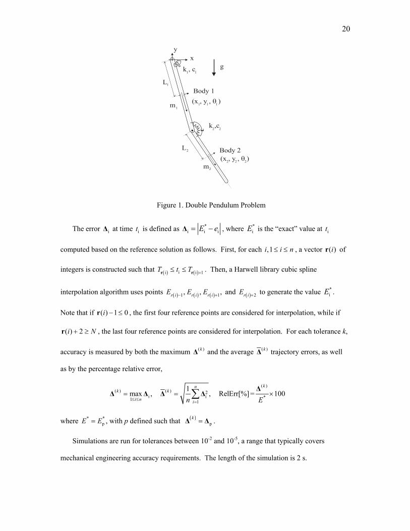
5.1. Validation of Proposed Algorithm. Validation is carried out using the double pendulum

mechanism shown in Fig. 1. Stiffness is induced by means of two rotational spring-damper-

actuators (RSDA). Masses of the pendulum bodies are 1m = 3 and 2m = 0.3, dimensions are 1L

= 1 and 2L = 1.5, stiffness coefficients are 1k = 400 and 2k = 53 10⋅ , and damping coefficients

are 1C = 15 and 2C = 45 10⋅ , all units in SI. Note that the zero-tension angles for the two RSDA

19

elements are 01 3 2α π= and 0

2α = 0. In its initial configuration, the two-degree of freedom

dynamic system has a dominant eigenvalue with a small imaginary part (less than 410− ) and a

real part of the order 510− . Since the bodies are connected through two parallel revolute joints,

the problem is planar. In terms of initial conditions, the centers of mass (CM) of bodies 1 and 2

are located at 1 1CMx = , 1 0CMy = and 2 3.4488887CMx = , 2 0.388228CMy = − . In the initial

configuration, the centroidal principal reference frame of body 1 is parallel with the global

reference frame, while the centroidal principal reference frame of body 2 is rotated by

2 23 12θ π= about an axis perpendicular on the plane of motion. For body 1,

1 1 1 0CM CM CMx y θ= = = , while for body 2, 2 3.8822857CMx = , 2 14.488887CMy = , and 2 10CMθ = .

Note that all initial conditions are in SI units and are consistent with the kinematic constraint

equations at position and velocity levels (Eqs. (2) and (3)).

For validation, simulations are run with several tolerances, and the results are analyzed to see

if imposed accuracy requirements are met. A reference solution is first generated by imposing a

very tight tolerance. All simulations are compared to the reference simulation, to find the infinity

norm of the error, the time at which it occurs, and the average error per time step.

Suppose that n time steps are taken during the current simulation, and the variable used for

error analysis is denoted by e . The grid points of the current simulation are denoted by

1 2init n endt t t t t= < < < =… , and results of the current simulation are obtained as ie , for 1 i n≤ ≤ .

If N is the number of time steps taken during the reference simulation, it is expected that N n>> .

Let 1initT T= <… N endT T< = be the simulation time steps, and jE , 1 j N≤ ≤ , be the

corresponding reference values.

20

Figure 1. Double Pendulum Problem

The error i∆ at time it is defined as *i i iE e= −∆ , where *

iE is the “exact” value at it

computed based on the reference solution as follows. First, for each , 1i i n≤ ≤ , a vector ( )ir of

integers is constructed such that ( ) ( )ii i 1T t T +≤ ≤r r . Then, a Harwell library cubic spline

interpolation algorithm uses points ( ) ( ) ( )1 1, , , r i r i r iE E E− + and ( ) 2r iE + to generate the value *iE .

Note that if ( ) 1 0i − ≤r , the first four reference points are considered for interpolation, while if

( ) 2i N+ ≥r , the last four reference points are considered for interpolation. For each tolerance k,

accuracy is measured by both the maximum ( )k∆ and the average ( )k∆ trajectory errors, as well

as by the percentage relative error,

( )( ) ( ) 2

i i *1 1

1max , , RelErr[%] = 100

knk k

i n in E≤ ≤ =

= = ×∑ ∆∆ ∆ ∆ ∆

where * *pE E= , with p defined such that ( )

pk =∆ ∆ .

Simulations are run for tolerances between 10-2 and 10-5, a range that typically covers

mechanical engineering accuracy requirements. The length of the simulation is 2 s.

21

Figure 2 presents the time variation of orientation angle 1θ and the time variation of angular

velocity 1θ for body 1. The length of the reference simulation; i.e., the length for which error

analysis is carried out, is T = 2 s. With an integration tolerance of 810− , the code takes 678

successful time steps to run 2 s of simulation.

Table II contains results of error analysis at position and velocity levels. The first column

contains the value of the tolerance with which the simulation is run. Relative and absolute

tolerances for the step-size control mechanism are set to 10k , and they apply for both position

and velocity. The second column contains the time t∗ at which the largest error ( )k∆ occurred.

The third column contains ( )k∆ . Column four contains the relative error. Column five contains

the average error per time step. The most relevant information for method validation is ( )k∆ . If

3k = − ; i.e., accuracy of 10-3 is demanded, ( 3)−∆ should have this order of magnitude. It can be

seen in Table II that this is the case for all tolerances, except for the case 5k = − , where the

magnitude of the error is close to order 410− . One reason for which the value of k is not always

reflected exactly in the value of ( )k∆ is that the relative tolerance comes into play. For this

experiment, the nonzero iRtol loosens the accuracy of the solution, proportional to the magnitude

of the variable controlled. Based on results shown in Fig. 2, the relative tolerance is multiplied by

a value that oscillates between 4.0 and 6.0. Therefore, the actual upper bound of accuracy

imposed on the solution fluctuates and reaches values up to 7 10 k−⋅ .

22

-10

-7

-4

-1

2

5

8

0 2 4 6 8 10

Time [s]

Ang

le [r

ad],

Ang

le_d

ot[r

ad/s

]Theta1 Theta1_dot

Figure 2. Time Variation of Orientation and Angular Velocity for Body 1

Position Velocity

k t ∗ ∆ ( )k RelErr

[%] ∆ ( )k t ∗ ∆ ( )k

RelErr

[%] ∆ ( )k

-2 0.413557 3.280E-2 0.887 1.147E-3 0.578444 2.290E-1 3.841 8.375E-3

-3 0.425395 3.787E-3 0.103 1.111E-4 0.291094 3.131E-2 0.428 9.066E-4

-4 0.351082 7.546E-4 0.020 1.966E-5 0.551010 6.407E-3 0.119 1.531E-4

-5 1.084304 1.706E-4 0.004 4.211E-6 0.136235 1.485E-3 0.017 3.502E-5

Table II. Position and Velocity Error Analysis for the Double Pendulum Problem

Error analysis is also performed at the velocity level. The angular velocity of body 1

fluctuates between –10 and 7 rad/s. The absolute and relative tolerances were set to 10k ,

2, , 5k = − −… , for all numerical experiments. The order of magnitude for ( )k∆ is expected to be

110k+ , and results in Table II confirm theoretical predictions.

Results presented in this Section confirm reliability of the step-size controller. While slightly

on the optimistic side, the step-size controller shows that the idea of using an embedded formula

for local error estimation is sound. Accuracy obtained with the algorithm is good.

23

For the 2 s double pendulum simulation, Table III contains a comparison between the number

of integration steps taken by the original SDIRK4/15 (ODE) code, and by the proposed SSODE

algorithm. The difference in the number of steps comes form the different settings used for the

integrator in the SSODE algorithm. In the ODE formulation, the code is used with the original

settings, and the equations of motion are expressed in terms of the angles 1θ and 2θ .

k -2 -3 -4 -5 -6 -7 -8

ODE 31 47 76 127 223 387 682

SSODE 29 47 75 126 219 384 678

Table III. Number of Steps for ODE and SSODE algorithms

5.2. Performance Comparison with Explicit Integrator. The algorithm presented has been

tested using a model of the US Army High Mobility Multipurpose Wheeled Vehicle (HMMWV).

The HMMWV shown in Fig.3 is modeled using 14 bodies, as shown in Fig. 4. In this figure,

vertices represent bodies, while edges represent joints connecting the bodies of the system.

Vertex number 1 is the chassis, 3 and 6 are the right and left lower control arms, 2 and 5 are the

right and left front upper control arms, 9 and 12 are the right and left rear lower control arms, and

8 and 11 are the right and left upper control arms. Bodies 4, 7, 10, and 13 are the wheel spindles,

and body 14 is the steering rack. Spherical joints are denoted by S, revolute joints by R, distance

constraints by D, and translational joints by T. This set of joints imposes 79 constraint equations.

One additional constraint equation is imposed on the steering system, such that the steering angle

is zero; i.e., the vehicle drives straight. A total of 98 generalized coordinates are used to model

the vehicle, which has 18 degrees of freedom.

24

Figure 3. HMMWV Figure 4. HMMWV Model Representation

Stiffness is induced in the model by means of four translational spring-damper actuators

(TSDA) that represent suspension bushings. These TSDAs act between the front/rear and

left/right upper control arms and the chassis. The stiffness coefficient of each TSDA is

72 10 N/m⋅ , while the damping coefficient is 62 10 Ns/m⋅ . For the purpose of this numerical

experiment, the tires of the vehicle are modeled as vertical TSDA elements with stiffness

coefficient 296,325 N/m and damping coefficient 3,502 Ns/m . Finally, the dominant

eigenvalue of the SSODE of Eq. (19) has a real component of approximately 52.6 10− ⋅ , and a

small imaginary part (less than 410− ).

Dynamic analysis is carried out for the scenario in which the vehicle drives straight at 16

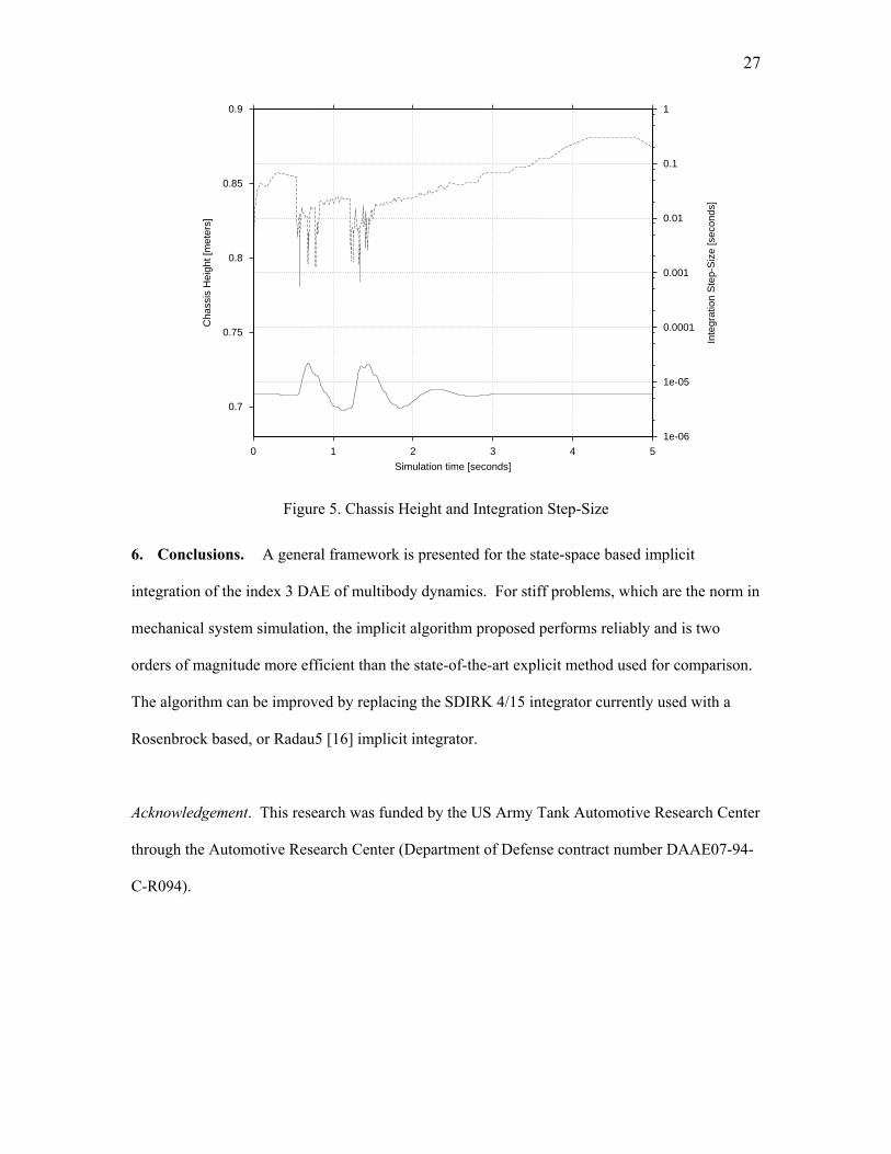
km/h over a bump. The shape of the bump is a half-cylinder of diameter 0.1m. Figure 5 shows

the time variation of the vehicle chassis height. The front wheels hit the bump at 0.5T ≈ s, and

the rear wheels hit the bump at 1.2T ≈ s. The duration of the simulation in this plot is 5 s.

Toward the end of the simulation (after 4 s), due to over-damping, the chassis height stabilizes at

approximately 1 0.71z = m.

25

The test problem is first run with an explicit integrator, based on the code DEABM [31]. The

explicit integration approach used for the equations of motion for the HMMWV model is outlined

in Table IV. The first 3 steps are identical to the ones in the algorithm of Table I. Step 4

computes the acceleration q . A topology-based approach [29] that takes into account sparsity of

the coefficient matrix is used to solve for q . The DDEABM integrator is then used to integrate

for independent velocities nv and independent positions nv . The integrator is also used to

integrate for dependent coordinates nu , with the sole purpose of providing a good starting point

during Step 6 for the iterative solver. At each time step nt , nu is computed by ensuring that the

kinematic position constraint equations are satisfied; i.e., solving ( )n nΦ v ,u = 0 . Likewise,

dependent velocities nu are the solution of the linear system ( ) ( )n n n n n nu vΦ v ,u u = Φ v ,u v− ,

which thus guarantees that the generalized velocities satisfy the kinematic velocity constraint

equations. The dependent/independent partitioning of the generalized coordinates is checked

during Step 7, and the algorithm concludes one integration step and proceeds to the next.

Algorithm 2

1. Initialize Simulation

2. Set Integration Tolerance

3. While (time < time-end) do

4. Get Acceleration

5. Apply Integration Step. Check Accuracy. Determine New Step-size

6. Recover Dependent Generalized Coordinates

7. Check Partition; Increase simulation time

8. End do

Table IV. Explicit Integration Algorithm

Tables V and VI provide timing results for the algorithms implemented, obtained on an SGI

Onyx computer with an R10000 processor. The first column contains the duration of the

simulation. The first row indicates the value of the tolerance set for the simulation. The absolute

26

and relative tolerances for the step-size control mechanism are the same for all variables that are

integrated. Error control is done at both position and velocity levels. Timing results for the

explicit algorithm are provided in Table VI.

For the entire simulation, poor stability of the explicit algorithm limits the integration step-

size to values in the range of 610− to 510− s. Note that for the explicit integrator the CPU time

does not depend on the imposed error tolerance, an indication that in this range of tolerances

stability rather than accuracy considerations dictate the integration step-size.

Table V. Implicit Integrator Timing Results Table VI. Explicit Integrator Timing Results

for the HMMWV Problem for the HMMWV problem

Figure 5 shows the time variation of integration step-size when absolute and relative errors at

position and velocity levels are set to 310− . The y-axis for the step-size is provided at the right of

Fig. 5, on a logarithmic scale. The time variation of the chassis height is provided in the lower

half of the same figure, relative to the left y-axis. Note that when the vehicle hits the bump; i.e.,

when in Fig. 5 the z coordinate of the chassis increases suddenly, the step-size is decreased to

preserve accuracy of the numerical solution. On the other hand, for the region in which the road

becomes flat; i.e., toward the end of the simulation, the integrator is capable of taking larger

integration steps, thus decreasing CPU time. For the vehicle model considered, simulated under

mild accuracy requirements, the algorithm is approximately 150 times faster than the explicit

algorithm.

TOL 10-2 10-3 10-4 10-5 TOL 10-2 10-3 10-4 10-5

1 s 10.1 21 33 57 1 s 3618 3641 3667 3663

2 s 25.3 49 78 139 2 s 7276 7348 7287 7276

3 s 29.5 58 92 166 3 s 10865 11122 10949 10965

4 s 30 61 94 184 4 s 14480 14771 14630 14592

27

0.7

0.75

0.8

0.85

0.9

0 1 2 3 4 5

1e-06

1e-05

0.0001

0.001

0.01

0.1

1

Cha

ssis

Hei

ght [

met

ers]

Inte

grat

ion

Ste

p-S

ize

[sec

onds

]

Simulation time [seconds]

Figure 5. Chassis Height and Integration Step-Size

6. Conclusions. A general framework is presented for the state-space based implicit

integration of the index 3 DAE of multibody dynamics. For stiff problems, which are the norm in

mechanical system simulation, the implicit algorithm proposed performs reliably and is two

orders of magnitude more efficient than the state-of-the-art explicit method used for comparison.

The algorithm can be improved by replacing the SDIRK 4/15 integrator currently used with a

Rosenbrock based, or Radau5 [16] implicit integrator.

Acknowledgement. This research was funded by the US Army Tank Automotive Research Center

through the Automotive Research Center (Department of Defense contract number DAAE07-94-

C-R094).

REFERENCES

[1] Alishenas, T., Olafsson, O., “Modeling and Velocity Stabilization of Constrained Mechanical

Systems”, BIT 34, 1994, 455--483

[2] Ascher, U. M., Chin, H., Petzold, L. R., Reich, S., “Stabilization of Constrained Mechanical

Systems with DAEs and Invariant Manifolds”, Mech. Struct. & Mach. 23(2), 1995, 125—157

[3] Ascher, U. M., Petzold, L. R., “Stability of Computational Methods for Constrained

Dynamics Systems”, SIAM J. Sci., Stat. Comp. 14, 1993, 95--120

[4] Ascher, U. M., Petzold, L. R., Chin, H., “Stabilization of DAEs and Invariant Manifolds”

submitted to Numer. Math., 1994

[5] Atkinson, K. E., An Introduction to Numerical Analysis, John Wiley & Sons, 2nd Edition,

New York, 1989

[6] Baumgarte, J., “Stabilization of Constraints and Integrals of Motion in Dynamical Systems”,

Comp. Meth. In Appl. Mech. And Eng. 1, 1972, 1—16

[7] Brasey, V., “Half-Explicit Method for Semi-Explicit Differential-Algebraic Equations of

Index 2”, Thesis No. 2664, Sect. Math., University of Geneva, 1994

[8] Corwin, L. J., Szczarba, R. H., Multivariable Calculus, Marcel Dekker, New York, 1982

[9] De Jalon, J. G., Bayo, E., Kinematic and Dynamic Simulation of Multibody Systems: The

Real-time Challenge, Springer-Verlag, M.E. Series, New York, 1994

[10] Eich, E., Fuhrer, C., Leihmkuhler, B. J., Reich, S., “Stabilization and Projection Methods

for Multibody Dynamics”, Research Report A281, Helsinki University of Technology, Institute

of Mathematics, 1990

[11] Eich, E., “Convergence Results for a Coordinate Projective Method Applied to

Mechanical Systems with Algebraic Constraints”, SIAM J. Numer. Anal. 30, 1993, 1467--1482

[12] Fuhrer, C., Leihmkuhler, B. J., “Numerical Solution of DAEs for Constraint Mechanical

Motion”, Numerische Mathematik 59, 1991, 5—69

29

[13] Gear, C. W., Numerical Initial Value Problems in Ordinary Differential Equations,

Prentice Hall, Englewood Cliffs, NJ, 1971

[14] Gear, C. W., Gupta, G. K., Leihmkuhler, B. J., “Automatic Integration of the Euler-

Lagrange Equations with Constraints”, J. Comp. Appl. Math. 12 & 13, 1985, 77—90

[15] Hairer, E., Nørsett S. P., Wanner, G., Solving Ordinary Differential Equations I. Nonstiff

Problems, Springer-Verlag, Berlin, 1993

[16] Hairer, E., Wanner, G., Solving Ordinary Differential Equations II. Stiff and Differential-

Algebraic Problems, Springer-Verlag, Berlin, 1996

[17] Haug, E. J., Computer-Aided Kinematics and Dynamics of Mechanical Systems,

Prentice-Hall, Englewood Cliffs, NJ, 1989

[18] Lapack Users’ Guide, SIAM, Philadelphia, 1992

[19] Liang, C. G., Lance, G. M., “A Differentiable Null-Space Method for Constrained

Dynamics Analysis”, ASME J. of Mechanisms, Transmissions, and Automation in Design 109,

1987, 405--411

[20] Lubich, C., “Extrapolation Methods for Constrained Multibody Systems”, Technical

Report A-6020, University of Innsbruck, Institute for Mathematics and Geometry, 1990

[21] Lubich, C., Nowak, U., Pohle, U., Engstler, C., “MEXX-Numerical Software for the

Integration of Constrained Mechanical Multibody Systems”, Preprint SC 92-12, Konrad-Zuse

Zentrum, Berlin, 1992

[22] Mani, N. K., Haug, E. J., Atkinson, K. E., “Application of Singular Value Decomposition

for the Analysis of Mechanical System Dynamics”, ASME J. of Mechanism, Transmissions, and

Automation in Design 107, 1985, 82--87

[23] Negrut, D., “On the Implicit Integration of Differential-Algebraic Equations of

Multibody Dynamics”, Ph.D. Thesis, The University of Iowa, 1998

30

[24] Ostermeyer, G. P., “Baumgarte Stabilization for DAEs”, In NATO Advances Research

Workshop in Real-Time Integration Methods for Mechanical System Simulation, Haug E. and

Deyo R., eds, Springer Verlag, Berlin Heidelberg NY, 1990

[25] Petzold, L. R, “Differential-Algebraic Equations are not ODE’s”, SIAM J. Sci., Stat.

Comput. 3(3), 1982, 367—384

[26] Potra, F. A., Rheinboldt, W. C., “On the Numerical Solution of Euler-Lagrange

Equations”, Mech. Struct. & Mach. 19(1), 1991, 1--18

[27] Potra, F. A., “Implementation of Linear Multistep Methods for Solving Constrained

Equations of Motion”, SIAM Numer. Anal. 30(3), 1993, 474—489

[28] Serban, R., “Dynamic and Sensitivity Analysis of Multibody Systems”, Ph.D. Thesis,

The University of Iowa, 1998

[29] Serban, R., Negrut, D., Haug, E. J., Potra, F. A., "A Topology Based Approach for

Exploiting Sparsity in Multibody Dynamics in Cartesian Formulation”, Mech. Struct. & Mach.

25(3), 1997, 379—396

[30] Shampine, L. F., “Conservation Laws and the Numerical Solution of ODEs”, Comp. and

Math. with Appl. 12B, 1986, 1287--1296

[31] Shampine, L. F., Watts, H. A., “The art of writing a Runge-Kutta code. II”, Appl. Math.

Comput. 5, 1979, 93--121

[32] Wehage, R. A., Haug, E. J., “Generalized Coordinate Partitioning for Dimension

Reduction in Analysis of Constrained Systems”, J. Mech. Design 104, 1982, 247—255