123
Differential Equations 6 Copyright © Cengage Learning. All rights reserved. 6.1 6.2 6.3 6.4
| Date post: | 03-Jan-2016 |
| Category: |
Documents |
| Upload: | lorraine-pamela-wiggins |
| View: | 236 times |
| Download: | 2 times |

Differential Equations6
Copyright © Cengage Learning. All rights reserved.
6.16.26.36.4

2
First-Order Linear Differential Equations
Copyright © Cengage Learning. All rights reserved.
6.4

3
Solve a first-order linear differential equation.
Use linear differential equations to solve applied problems.
Solve a Bernoulli differential equation.
Objectives

4
First-Order Linear Differential Equations

5
First-Order Linear Differential Equations

6
To solve a linear differential equation, write it in standard form to identify the functions P(x) and Q(x).
Then integrate P(x) and form the expression
which is called an integrating factor. The general solution of the equation is
First-Order Linear Differential Equations

7
Example 1 – Solving a Linear Differential Equation
Find the general solution of y' + y = ex.
Solution:For this equation, P(x) = 1 and Q(x) = ex.
So, the integrating factor is

8
Example 1 – Solutioncont’d
This implies that the general solution is

9
First-Order Linear Differential Equations

10
Example 2 – Solving a First-Order Linear Differential Equation
Find the general solution of xy' – 2y = x2.
Solution:The standard form of the given equation is
y' + P(x)y = Q(x)
So, P(x) = –2/x, and you have

11
Example 2 – Solution
So, multiplying each side of the standard form by 1/x2 yields
cont’d

12
Several solution curves (for C = –2, –1, 0, 1, 2, 3, and 4) are shown in Figure 6.19.
Figure 6.19
Example 2 – Solutioncont’d

13
Applications

14
Example 4 – A Mixture Problem
A tank contains 50 gallons of a solution composed of 90% water and 10% alcohol. A second solution containing 50% water and 50% alcohol is added to the tank at the rate of 4 gallons per minute. As the second solution is being added, the tank is being drained at a rate of 5 gallons per minute, as shown in Figure 6.21. Assuming the solution in the tank is stirred constantly, how much alcohol is in the tank after 10 minutes?
Figure 6.21

15
Example 4 – Solution
Let y be the number of gallons of alcohol in the tank at any time t.
You know that y = 5 when t = 0.
Because the number of gallons of solution in the tank at any time is 50 – t, and the tank loses 5 gallons of solution per minute, it must lose [5/(50 – t)]y gallons of alcohol per minute.
Furthermore, because the tank is gaining 2 gallons of alcohol per minute, the rate of change of alcohol in the tank is given by

16
To solve this linear equation, let P(t) = 5/(50 – t) and obtain
Because t < 50, you can drop the absolute value signs and conclude that
So, the general solution is
Example 4 – Solutioncont’d

17
Because y = 5 when t = 0, you have
which means that the particular solution is
Finally, when t = 10, the amount of alcohol in the tank is
which represents a solution containing 33.6% alcohol.
Example 4 – Solutioncont’d

18
Bernoulli Equation

19
Bernoulli Equation
A well-known nonlinear equation that reduces to a linear one with an appropriate substitution is the Bernoulli equation, named after James Bernoulli (1654–1705).
This equation is linear if n = 0, and has separable variables if n = 1.
So, in the following development, assume that
n ≠ 0 and n ≠ 1.

20
Begin by multiplying by y–n and (1 – n) to obtain
which is a linear equation in the variable y1–n. Letting
z = y1–n produces the linear equation
Bernoulli Equation

21
Finally, by Theorem 6.3, the general solution of the Bernoulli equation is
Bernoulli Equation

22
Example 7 – Solving a Bernoulli Equation
Find the general solution of y' + xy = xe–x2y–3.
Solution:
For this Bernoulli equation, let n = –3, and use the substitution
z = y4 Let z = y1 – n = y1 – (–3).
z' = 4y3y'. Differentiate.

23
Example 7 – Solution
Multiplying the original equation by 4y3 producesy' + xy = xe–x2y–3. Write original equation.
4y3y' + 4xy4 = 4xe–x2 Multiply each side by 4y3.
z' + 4xz = 4xe–x2. Linear equation: z' + P(x)z = Q(x)
This equation is linear in z. Using P(x) = 4x produces
which implies that e2x2 is an integrating factor.
cont’d

24
Multiplying the linear equation by this factor produces
cont’dExample 7 – Solution

25
Finally, substituting z = y4 , the general solution is
cont’dExample 7 – Solution

26
Bernoulli Equation

Slope Fields and Euler’s Method
Copyright © Cengage Learning. All rights reserved.
6.1

28
Use initial conditions to find particular solutions of differential equations.
Use slope fields to approximate solutions of differential equations.
Use Euler’s Method to approximate solutions of differential equations.
Objectives

29
General and Particular Solutions

30
General and Particular Solutions
The physical phenomena can be described by differential equations.
A differential equation in x and y is an equation that involves x, y, and derivatives of y.
A function y = f(x) is called a solution of a differential equation if the equation is satisfied when y and its derivatives are replaced by f(x) and its derivatives.

31
General and Particular Solutions
For example, differentiation and substitution would show that y = e–2x is a solution of the differential equation
y' + 2y = 0.
It can be shown that every solution of this differential equation is of the form y = Ce–2x General solution of y ' + 2y = 0
where C is any real number.
This solution is called the general solution. Some differential equations have singular solutions that cannot be written as special cases of the general solution.

32
General and Particular Solutions
The order of a differential equation is determined by the highest-order derivative in the equation.
For instance, y' = 4y is a first-order differential equation.
The second-order differential equation s''(t) = –32 has the general solution
s(t) = –16t2 + C1t + C2 General solution of s''(t) = –32
which contains two arbitrary constants.
It can be shown that a differential equation of order n has a general solution with n arbitrary constants.

33
Example 1 – Verifying Solutions
Determine whether the function is a solution of
the differential equation y''– y = 0.
a. y = sin x b. y = 4e–x c. y = Cex
Solution:
a. Because y = sin x, y' = cos x, and y'' = –sin x, it follows that
y'' – y = –sin x – sin x = –2sin x ≠ 0.
So, y = sin x is not a solution.

34
Example 1 – Solution
b. Because y = 4e–x, y' = –4e–x, and y'' = 4e–x, it follows that
y'' – y = 4e–x – 4e–x= 0.
So, y = 4e–x is a solution.
c. Because y = Cex, y' = Cex, and y'' = Cex, it follows that
y'' – y = Cex – Cex= 0.
So, y = Cex is a solution for any value of C.
cont’d

35
General and Particular Solutions
Geometrically, the general solution of a first-order differential equation represents a family of curves known as solution curves, one for each value assigned to the arbitrary constant.
For instance, you can verify that every function of the form
is a solution of the differential equation xy' + y = 0.

36
Figure 6.1 shows four of the solution curves corresponding to different values of C.
Particular solutions of a differential
equation are obtained from initial
conditions that give the values of
the dependent variable or one of its
derivatives for particular values of
the independent variable.
Figure 6.1
General and Particular Solutions

37
The term “initial condition” stems from the fact that, often in problems involving time, the value of the dependent variable or one of its derivatives is known at the initial time t = 0.
For instance, the second-order differential equation
s''(t) = –32 having the general solution
s(t) = –16t2 + C1t + C2 General solution of s''(t) = –32
might have the following initial conditions.s(0) = 80, s'(0) = 64 Initial conditions
In this case, the initial conditions yield the particular solution
s(t) = –16t2 + 64t + 80. Particular solution
General and Particular Solutions
38
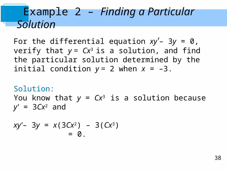
Example 2 – Finding a Particular Solution
For the differential equation xy'– 3y = 0, verify that y = Cx3
is a solution, and find the particular solution determined by the initial condition y = 2 when x = –3.
Solution:You know that y = Cx3 is a solution because y' = 3Cx2 and
xy'– 3y = x(3Cx2) – 3(Cx3) = 0.
39
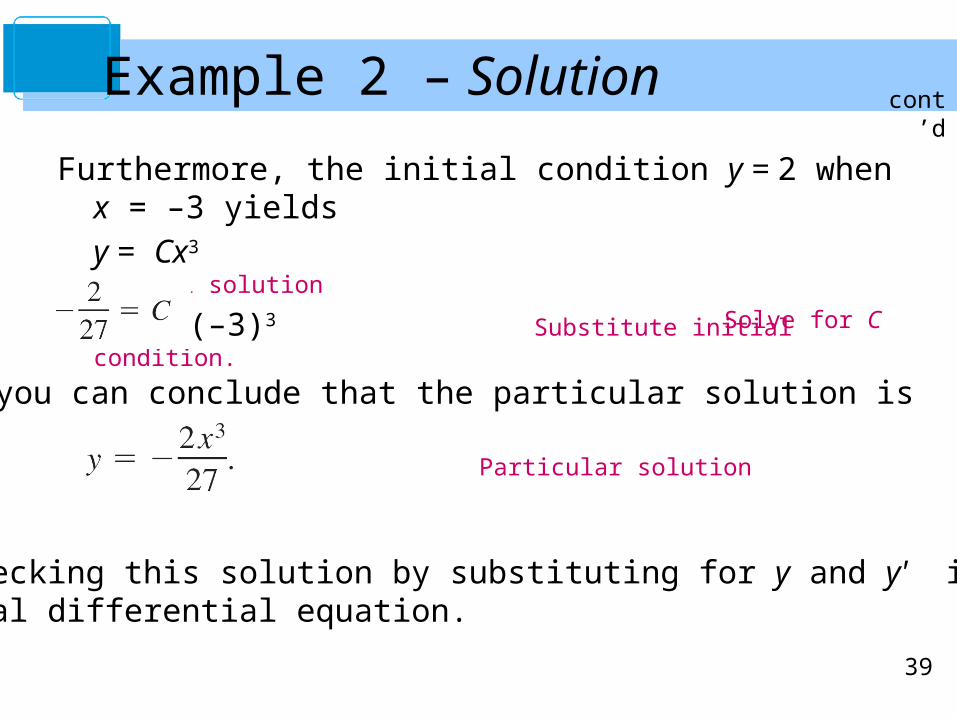
Example 2 – Solution
Furthermore, the initial condition y = 2 when x = –3 yieldsy = Cx3 General solution
2 = C(–3)3 Substitute initial condition.
Solve for C
Particular solution
and you can conclude that the particular solution is
Try checking this solution by substituting for y and y' in the original differential equation.
cont’d

40
Slope Fields

41
Slope Fields
Solving a differential equation analytically can be difficult or even impossible. However, there is a graphical approach you can use to learn a lot about the solution of a differential equation.
Consider a differential equation of the formy' = F(x, y) Differential equation
where F(x, y) is some expression in x and y.
At each point (x, y) in the xy–plane where F is defined, the differential equation determines the slope y' = F(x, y) of the solution at that point.

42
Slope Fields
If you draw short line segments with slope F(x, y) at selected points (x, y) in the domain of F, then these line segments form a slope field, or a direction field, for the differential equation y' = F(x, y).
Each line segment has the same slope as the solution curve through that point.
A slope field shows the general shape of all the solutions and can be helpful in getting a visual perspective of the directions of the solutions of a differential equation.

43
Example 3 – Sketching a Slope Field
Sketch a slope field for the differential equation y' = x – y
for the points (–1, 1), (0, 1), and (1, 1).
Solution:The slope of the solution curve at any point (x, y) is F (x, y) = x – y.
So, the slope at (–1, 1) is y' = –1 –1 = –2, the slope at
(0, 1) is y' = 0 – 1 = –1, and the slope at (1, 1) is
y' = 1 – 1 = 0.

44
Example 3 – Solution
Draw short line segments at the three points with theirrespective slopes, as shown in Figure 6.2.
Figure 6.2
cont’d

45
Euler’s Method

46
Euler’s Method
Euler’s Method is a numerical approach to approximating the particular solution of the differential equation
y' = F(x, y)
that passes through the point (x0, y0).
From the given information, you know that the graph of the solution passes through the point (x0, y0) and has a slope of
F(x0, y0) at this point.
This gives you a “starting point” for approximating the solution.

47
Euler’s Method
From this starting point, you can proceed in the direction indicated by the slope.
Using a small step h, move along the
tangent line until you arrive at the
point (x1, y1) where
x1 = x0 + h and y1 = y0 + hF(x0, y0) as shown in Figure 6.6.
Figure 6.6

48
Euler’s Method
If you think of (x1, y1) as a new starting point, you can
repeat the process to obtain a second point (x2, y2).
The values of xi and yi are as follows.

49
Example 6 – Approximating a Solution Using Euler’s Method
Use Euler’s Method to approximate the particular solution of the differential equation
y' = x – y
passing through the point (0, 1). Use a step of h = 0.1.
Solution:Using h = 0.1, x0 = 0, y0 = 1, and F(x, y) = x – y, you have x0 = 0, x1 = 0.1, x2 = 0.2, x3 = 0.3,…, and
y1 = y0 + hF(x0, y0) = 1 + (0.1)(0 – 1) = 0.9
y2 = y1 + hF(x1, y1) = 0.9 + (0.1)(0.1 – 0.9) = 0.82
y3 = y2 + hF(x2, y2) = 0.82 + (0.1)(0.2 – 0.82) = 0.758.

50
Example 6 – Solution
Figure 6.7
The first ten approximations are shown in the table.
cont’d
You can plot these values to see a
graph of the approximate solution,
as shown in Figure 6.7.

51
Differential Equations: Growth and Decay
Copyright © Cengage Learning. All rights reserved.
6.2

52
Use separation of variables to solve a simple differential equation.
Use exponential functions to model growth and decay in applied problems.
Objectives

53
Differential Equations

54
Differential Equations
Analytically, you have learned to solve only two types of
differential equations—those of the forms
y' = f(x) and y'' = f(x).
In this section, you will learn how to solve a more general
type of differential equation.
The strategy is to rewrite the equation so that each variable
occurs on only one side of the equation. This strategy is
called separation of variables.

55
Example 1 – Solving a Differential Equation
So, the general solution is given by y2 – 2x2 = C.

56
Growth and Decay Models
57
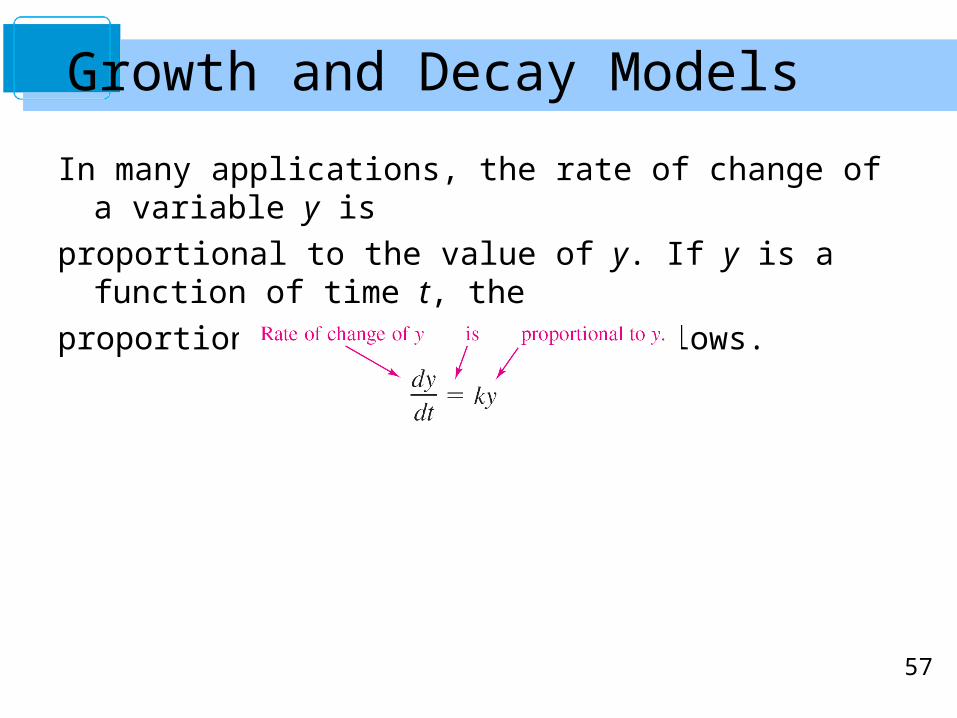
Growth and Decay Models
In many applications, the rate of change of a variable y is
proportional to the value of y. If y is a function of time t, the
proportion can be written as follows.

58
The general solution of this differential equation is given inthe following theorem.
Growth and Decay Models

59
Example 2 – Using an Exponential Growth Model
The rate of change of y is proportional to y. When t = 0,
y = 2, and when t = 2, y = 4. What is the value of y when t = 3?
Solution:
Because y' = ky, you know that y and t are related by the
equation y = Cekt.
You can find the values of the constants C and k by applying the initial conditions.

60
Example 2 – Solutioncont'd
So, the model is y ≈ 2e0.3466t .
When t = 3, the value of y is 2e0.3466(3) ≈ 5.657
(see Figure 6.8).
Figure 6.8

61
You did not actually have to solve the differential equation
y' = ky.
The next example demonstrates a problem whose
solution involves the separation of variables technique.
The example concerns Newton's Law of Cooling, which
states that the rate of change in the temperature of an
object is proportional to the difference between the
object’s temperature and the temperature of the
surrounding medium.
Growth and Decay Models

62
Example 6 – Newton's Law of Cooling
Let y represent the temperature (in ºF) of an object in a room whose temperature is kept at a constant 60º. If the object cools from 100º to 90º in 10 minutes, how much longer will it take for its temperature to decrease to 80º?
Solution:
From Newton's Law of Cooling, you know that the rate of change in y is proportional to the difference between y and 60.
This can be written as
y' = k(y – 60), 80 ≤ y ≤ 100.

63
Example 6 – Solution
To solve this differential equation, use separation of variables, as follows.
cont'd

64
Because y > 60, |y – 60| = y – 60, and you can omit the absolute value signs.
Using exponential notation, you have
Using y = 100 when t = 0, you obtain
100 = 60 + Cek(0) = 60 + C, which implies that C = 40.
Because y = 90 when t = 10,
90 = 60 + 40ek(10)
30 = 40e10k
Example 6 – Solutioncont'd

65
So, the model is y = 60 + 40e–0.02877t Cooling model
and finally, when y = 80, you obtain
So, it will require about 14.09 more minutes for the object
to cool to a temperature of 80º (see Figure 6.11).
Figure 6.11
Example 6 – Solutioncont'd

66
Separation of Variables and the Logistic Equation
Copyright © Cengage Learning. All rights reserved.
6.3
67
Recognize and solve differential equations that can be solved by separation of variables.
Recognize and solve homogeneous differential equations.
Use differential equations to model and solve applied problems.
Solve and analyze logistic differential equations.
Objectives

68
Separation of Variables

69
Separation of Variables
Consider a differential equation that can be written in the form
where M is a continuous function of x alone and N is a continuous function of y alone. For this type of equation, all x terms can be collected with dx and all y terms with dy, and a solution can be obtained by integration.
Such equations are said to be separable, and the solution procedure is called separation of variables.

70
Below are some examples of differential equations that are separable.
Separation of Variables

71
Example 1 – Separation of Variables
Find the general solution of
Solution:
To begin, note that y = 0 is a solution.
To find other solutions, assume that y ≠ 0 and separate variables as shown.
Now, integrate to obtain

72
Example 1 – Solutioncont'd
Because y = 0 is also a solution, you can write the general solution as

73
Homogeneous Differential Equations

74
Homogeneous Differential Equations
Some differential equations that are not separable in x and y can be made separable by a change of variables.
This is true for differential equations of the form y' = f(x, y), where f is a homogeneous function.
The function given by f(x, y) is homogeneous of degree n if
where n is an integer.

75
Example 4 – Verifying Homogeneous Functions
a. f(x, y) = x2y – 4x3 + 3xy2 is a homogeneous function of degree 3 because
f(tx, ty) = (tx)2(ty) – 4(tx)3 + 3(tx)(ty)2
= t 3(x2y) – t
3(4x3) + t 3(3xy2)
= t 3(x2y – 4x3 + 3xy2)
= t 3f(x, y).
b. f(x, y) = xex/y + y sin(y/x) is a homogeneous function of degree 1 because

76
Example 4 – Verifying Homogeneous Functions
c. f(x, y) = x + y2 is not a homogeneous function because f(tx, ty) = tx + t2y2
= t(x + ty2)
≠ tn(x + y2).
d. f(x, y) = x/y is a homogeneous function of degree 0 because
cont'd

77
Homogeneous Differential Equations

78
Example 5 – Testing for Homogeneous Differential Equations
a. (x2 + xy)dx + y2dy = 0 is homogeneous of degree 2.
b. x3dx = y3dy is homogeneous of degree 3.
c. (x2 + 1)dx + y2dy = 0 is not a homogeneous differential
equation.

79
Homogeneous Differential Equations
To solve a homogeneous differential equation by the method of separation of variables, use the following change of variables theorem.

80
Example 6 – Solving a Homogeneous Differential Equation
Find the general solution of (x2 – y2)dx + 3xydy = 0.
Solution:
Because (x2 – y2) and 3xy are both homogeneous of degree 2, let y = vx to obtain dy = xdv + vdx.
Then, by substitution, you have

81
Example 6 – Solution
Dividing by x2 and separating variables produces
cont'd

82
Example 6 – Solution
Substituting for v produces the following general solution.
You can check this by differentiating and rewriting to get the original equation.
cont'd

83
Applications

84
Example 7 – Wildlife Population
The rate of change of the number of coyotes N(t) in a
population is directly proportional to 650 – N(t), where t is
the time in years. When t = 0, the population is 300, and
when t = 2, the population has increased to 500. Find the
population when t = 3.

85
Example 7 – Solution
Because the rate of change of the population is proportional to 650 – N(t), you can write the following differential equation.
You can solve this equation using separation of variables.
cont'd

86
Example 7 – Solution
Using N = 300 when t = 0, you can conclude that C = 350, which produces
N = 650 – 350e –kt.
Then, using N = 500 when t = 2, it follows that
500 = 650 – 350e –2k k ≈ 0.4236.
So, the model for the coyote population is
N = 650 – 350e –0.4236t.
cont'd

87
Example 7 – Solution
When t = 3, you can approximate the population to be
N = 650 – 350e –0.4236(3) ≈ 552 coyotes.
The model for the population is shown in Figure 6.14.
Note that N = 650 is the horizontalasymptote of the graph and is thecarrying capacity of the model. Figure 6.14
cont'd

88
Applications
A common problem in electrostatics, thermodynamics, and hydrodynamics involves finding a family of curves, each of which is orthogonal to all members of a given family of curves. For example, Figure 6.15 shows a family of circles
x2 + y2 = C Family of circles
each of which intersects the lines in the family
y = Kx Family of Lines
at right angles.Figure 6.15

89
Two such families of curves are said to be mutually orthogonal, and each curve in one of the families is called an orthogonal trajectory of the other family.
In electrostatics, lines of force are orthogonal to the equipotential curves.
In thermodynamics, the flow of heat across a plane surface is orthogonal to the isothermal curves.
In hydrodynamics, the flow (stream) lines are orthogonal trajectories of the velocity potential curves.
Applications

90
Example 8 – Finding Orthogonal Trajectories
Describe the orthogonal trajectories for the family of curves given by
for C ≠ 0. Sketch several members of each family.
Solution:
First, solve the given equation for C and write xy = C.
Then, by differentiating implicitly with respect to x, you obtain the differential equation
91
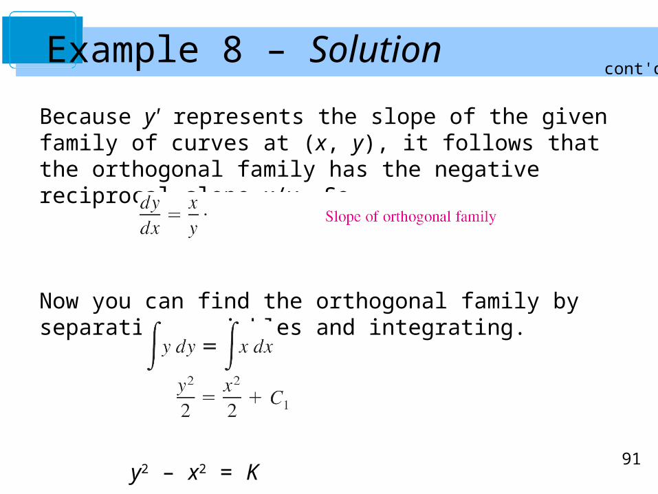
Because y' represents the slope of the given family of curves at (x, y), it follows that the orthogonal family has the negative reciprocal slope x/y. So,
Now you can find the orthogonal family by separating variables and integrating.
y2 – x2 = K
Example 8 – Solutioncont'd

92
Example 8 – Solution
The centers are at the origin, and the transverse axes arevertical for K > 0 and horizontal for K < 0.
If K = 0, the orthogonal trajectories are the lines y = ±x.If K ≠ 0, the orthogonal trajectories are hyperbolas.
Several trajectories are shownin Figure 6.16.
Figure 6.16
cont'd

93
Logistic Differential Equation
94
Logistic Differential Equation
The exponential growth model was derived from the fact that the rate of change of a variable y is proportional to the value of y.
You observed that the differential equation dy/dt = ky has the general solution y = Cekt.
Exponential growth is unlimited, but when describing a population, there often exists some upper limit L past which growth cannot occur. This upper limit L is called the carrying capacity, which is the maximum population y(t) that can be sustained or supported as time t increases.

95
Logistic Differential Equation
A model that is often used to describe this type of growth is the logistic differential equation
where k and L are positive constants. A population that satisfies this equation does not grow without bound, but approaches the carrying capacity L as t increases.
From the equation, you can see that if y is between 0 and the carrying capacity L, then dy/dt > 0, and the population increases.

96
Logistic Differential Equation
If y is greater than L, then dy/dt < 0, and the population decreases. The graph of the function y is called the logistic curve, as shown in Figure 6.17.
Figure 6.17

97
Example 9 – Deriving the General Solution
Solve the logistic differential equation
Solution: Begin by separating variables.

98
Example 9 – Solution
Solving this equation for y produces y =
cont'd
99
First-Order Linear Differential Equations
Copyright © Cengage Learning. All rights reserved.
6.4

100
Solve a first-order linear differential equation.
Use linear differential equations to solve applied problems.
Solve a Bernoulli differential equation.
Objectives

101
First-Order Linear Differential Equations

102
First-Order Linear Differential Equations

103
To solve a linear differential equation, write it in standard form to identify the functions P(x) and Q(x).
Then integrate P(x) and form the expression
which is called an integrating factor. The general solution of the equation is
First-Order Linear Differential Equations

104
Example 1 – Solving a Linear Differential Equation
Find the general solution of y' + y = ex.
Solution:For this equation, P(x) = 1 and Q(x) = ex.
So, the integrating factor is

105
Example 1 – Solutioncont’d
This implies that the general solution is

106
First-Order Linear Differential Equations

107
Example 2 – Solving a First-Order Linear Differential Equation
Find the general solution of xy' – 2y = x2.
Solution:The standard form of the given equation is
y' + P(x)y = Q(x)
So, P(x) = –2/x, and you have
108
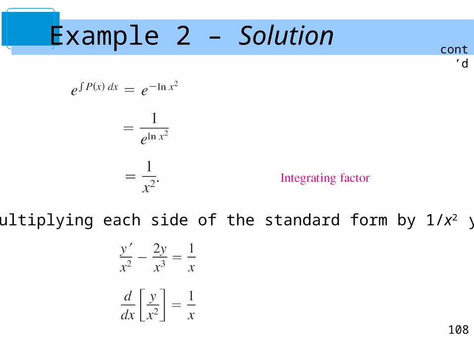
Example 2 – Solution
So, multiplying each side of the standard form by 1/x2 yields
cont’d

109
Several solution curves (for C = –2, –1, 0, 1, 2, 3, and 4) are shown in Figure 6.19.
Figure 6.19
Example 2 – Solutioncont’d
110
Applications

111
Example 4 – A Mixture Problem
A tank contains 50 gallons of a solution composed of 90% water and 10% alcohol. A second solution containing 50% water and 50% alcohol is added to the tank at the rate of 4 gallons per minute. As the second solution is being added, the tank is being drained at a rate of 5 gallons per minute, as shown in Figure 6.21. Assuming the solution in the tank is stirred constantly, how much alcohol is in the tank after 10 minutes?
Figure 6.21

112
Example 4 – Solution
Let y be the number of gallons of alcohol in the tank at any time t.
You know that y = 5 when t = 0.
Because the number of gallons of solution in the tank at any time is 50 – t, and the tank loses 5 gallons of solution per minute, it must lose [5/(50 – t)]y gallons of alcohol per minute.
Furthermore, because the tank is gaining 2 gallons of alcohol per minute, the rate of change of alcohol in the tank is given by

113
To solve this linear equation, let P(t) = 5/(50 – t) and obtain
Because t < 50, you can drop the absolute value signs and conclude that
So, the general solution is
Example 4 – Solutioncont’d

114
Because y = 5 when t = 0, you have
which means that the particular solution is
Finally, when t = 10, the amount of alcohol in the tank is
which represents a solution containing 33.6% alcohol.
Example 4 – Solutioncont’d

115
Bernoulli Equation

116
Bernoulli Equation
A well-known nonlinear equation that reduces to a linear one with an appropriate substitution is the Bernoulli equation, named after James Bernoulli (1654–1705).
This equation is linear if n = 0, and has separable variables if n = 1.
So, in the following development, assume that
n ≠ 0 and n ≠ 1.
117
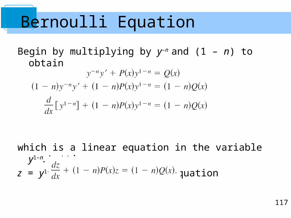
Begin by multiplying by y–n and (1 – n) to obtain
which is a linear equation in the variable y1–n. Letting
z = y1–n produces the linear equation
Bernoulli Equation

118
Finally, by Theorem 6.3, the general solution of the Bernoulli equation is
Bernoulli Equation

119
Example 7 – Solving a Bernoulli Equation
Find the general solution of y' + xy = xe–x2y–3.
Solution:
For this Bernoulli equation, let n = –3, and use the substitution
z = y4 Let z = y1 – n = y1 – (–3).
z' = 4y3y'. Differentiate.

120
Example 7 – Solution
Multiplying the original equation by 4y3 producesy' + xy = xe–x2y–3. Write original equation.
4y3y' + 4xy4 = 4xe–x2 Multiply each side by 4y3.
z' + 4xz = 4xe–x2. Linear equation: z' + P(x)z = Q(x)
This equation is linear in z. Using P(x) = 4x produces
which implies that e2x2 is an integrating factor.
cont’d

121
Multiplying the linear equation by this factor produces
cont’dExample 7 – Solution

122
Finally, substituting z = y4 , the general solution is
cont’dExample 7 – Solution

123
Bernoulli Equation


